Mergers,brandcompetition,andtheprice ofapint online at EuropeanEconomicReview48(2004)617–643 Mergers,brandcompetition,andtheprice ofapint JorisPinksea,MargaretE.Sladeb;∗ aDepartmentofEconomics

Available online at www.sciencedirect.com

European Economic Review 48 (2004) 617–643www.elsevier.com/locate/econbase

Mergers, brand competition, and the priceof a pint

Joris Pinksea, Margaret E. Sladeb;∗aDepartment of Economics, The Pennsylvania State University, University Park, PA, USA

bDepartment of Economics, The University of Warwick, Coventry CV4 7AL, UK

Received 31 August 2001; accepted 9 September 2002

Abstract

Mergers in the UK brewing industry have reduced the number of national brewers from sixto four. The number of brands, in contrast, has remained relatively constant. We analyze thee4ects of mergers on brand competition and pricing. Brand-level demand equations are estimatedfrom a panel of draft beers. To model brand-substitution possibilities, we estimate the matrixof cross-price elasticities semiparametrically. Our structural model is used to assess the strengthof brand competition along various dimensions and to evaluate the mergers. In particular, wecompute equilibria of pricing games with di4erent numbers of players.c© 2003 Elsevier B.V. All rights reserved.

JEL classi#cation: L13; L41; L66; L81

Keywords: Beer; Mergers; Brand competition; Di4erentiated products; Semiparametric instrumental-variableestimation

1. Introduction

Historically, the UK brewing industry was relatively unconcentrated. The last decade,however, has witnessed a succession of successful mergers that have increased con-centration in the industry, as well as proposed mergers that, if successful, would haveadded to that trend. It is thus natural to ask how those mergers have changed bothproduct pricing and product o4erings. In particular, the mergers could have resulted inhigher prices, a reduction in the number of brands, an increase in brand uniformity,and a move towards competition through national advertising. In this paper, we attempt

∗ Corresponding author. Fax: 2479-523-032.E-mail address: [email protected] (M.E. Slade).

0014-2921/$ - see front matter c© 2003 Elsevier B.V. All rights reserved.doi:10.1016/S0014-2921(02)00328-8

mailto:[email protected]

618 J. Pinkse, M.E. Slade / European Economic Review 48 (2004) 617–643

to assess the e4ects of actual mergers and to predict how unsuccessful mergers wouldhave a4ected the industry. Our formal analysis is limited to price changes, but weanalyze other consequences informally.Our merger evaluations are based on a structural model of demand, cost, and market

equilibrium. In particular, we estimate the demand for brands of a di4erentiated productand we use our estimated demands, together with engineering data on costs, to predictequilibrium prices and margins, which we compare to those that were observed. Wethen assess the e4ects of the mergers by solving for equilibria of games with di4er-ent numbers of players. In other words, changes in market structure – mergers anddivestitures – are modeled as changes in the number of decision makers, where eachdecision maker controls the prices of some set of brands. This means that when twoDrms merge, some pricing externalities are internalized. Moreover, if brands of the dif-ferentiated product are demand substitutes and prices are strategic complements, pricesrise after a merger. The question is: by how much do they rise?The use of econometric and simulation techniques for merger analysis is becoming

increasingly common. Indeed, competition authorities on both sides of the Atlantic rec-ognize the advantages of supplementing traditional merger analysis with quantitativeassessments. In this paper, we provide such an assessment for the UK brewing indus-try. We use panel data on all brands of beer that constitute at least one half of onepercent of a regional market to estimate the demand for brands of draft beers sold intwo regions of the country (Greater London and Anglia), two bimonthly time peri-ods (August/September and October/November 1995), and two types of establishments(multiples and independents).A number of classes of demand models have been used in merger-assessment

exercises, including the logit, nested logit, and random-coeHcients discrete-choicespeciDcations. 1 In contrast to those studies, our demand model is a continuous-choicespeciDcation. In particular, we extend the spatial model of Pinkse et al. (2002) to en-compass substitution among brands, and we estimate the matrix of cross-price elastici-ties semiparametrically as a function of a number of measures of the distance betweenbrands in product-characteristic space. We believe that our speciDcation combines thesimplicity of the logit and nested logit with the Iexibility of the random coeHcients.Furthermore, it can encompass endogeneity and measurement error in a straightforwardfashion.In the next section, we set the stage by describing the structure of the UK brewing

industry and some recent positions taken by UK competition authorities that havea4ected the industry’s horizontal-market structure. This is followed by a review of themerger-evaluation literature and the development of our model of demand, cost, andequilibrium. Our model is then used to assess two mergers – one that was allowed andone that was prohibited. To anticipate, we Dnd that the Scottish–Courage merger hadlittle e4ect on prices, whereas the proposed merger between Bass and Carlsberg–Tetleywould have resulted in more substantial price increases.

1 For example, Werden and Froeb (1994), Ivaldi and Verboven (2000), and Nevo (2000) evaluate mergersusing logit, nested-logit, and random-coeHcient demand models, respectively.

J. Pinkse, M.E. Slade / European Economic Review 48 (2004) 617–643 619

2. The UK beer market

To get a feel for the UK industry, it is useful to begin with some internationalcomparisons. Among Western countries, the UK is not an outlier with respect to con-sumption of beer per head or the fraction of sales that are imported. It is very di4erent,however, with respect to the ratio of draft to total beer sales. Indeed, draft sales in theUK, which in 1995 were about 70% of the total, accounted for almost three times thecomparable percentages in France and Germany and about six times the percentagesin North America. 2

Substantial changes in both consumption and production have occurred in the UKindustry in the last few decades. With respect to production, the number of brewershas declined steadily. Indeed, in 1900, there were nearly 1,500 brewery companies,but this number fell dramatically and is currently around Dfty. 3 However, in spite ofthe reduction in the number of brewers, prior to the mergers the UK industry wassubstantially less concentrated than its counterparts in the US, Canada, and France,where beer tends to be mass produced. Production in Germany, in contrast, wherespecialty beers predominate, was much less concentrated.Changes in tastes have also occurred. To illustrate, beers can be divided into three

broad categories: ales, stouts, and lagers. Although UK consumers traditionally pre-ferred ales, the consumption of lager has increased at a rapid pace. Indeed, from lessthan 1% of the market in 1960, lager became the dominant drink in 1990, when it be-gan to sell more than ale and stout combined. Most of those lagers are foreign brandsthat are brewed under license in the UK.A second important aspect of beer consumption is the popularity of ‘real’ or cask-

conditioned ale. Real products are alive and undergo a second fermentation in the cask,whereas keg and tank products are sterilized. Although real products’ share of the alemarket has increased, as a percentage of the total beer market, which includes lager,they have lost ground.A Dnal trend in consumption is the rise in popularity of premium beers, which are

deDned as brands with alcohol contents in excess of 4.2%. Traditional ales are of lowerstrength than stouts and lagers, and keg products tend to contain less alcohol than realproducts. Many of the more recently introduced brands, however, particularly the lagersand hybrid ales, are premium beers with relatively high alcohol contents.This snapshot of the UK beer industry shows signiDcant changes in tastes and con-

sumption habits as well as a decline in the number of companies that cater to thosetastes. Nevertheless, compared to many other countries, the UK brewing sector wasonly moderately concentrated. Recent developments in the industry, however, haveresulted in substantial changes in ownership patterns.In 1990, there were six national brewers: Bass, Allied Lyons, Scottish & Newcastle,

Grand Metropolitan (Grand Met), Courage, and Whitbread. Moreover, those six Drmshad dominated the market for decades. Since 1990, however, a sequence of mergershas increased concentration in brewing. First, three large mergers were approved by

2 Only in Ireland was it higher, where draft sales accounted for over 80% of consumption.3 In addition to incorporated brewers, there are over 100 microbreweries operating at very small scales.


UK competition authorities: Courage and Grand Met merged to form Courage, AlliedLyons and Carlsberg merged to form Carlsberg–Tetley, and Courage and Scottish &Newcastle merged to form Scottish Courage. After 1995, however, horizontal-mergerpolicy became less lenient. Indeed, a proposed merger between Bass and Carlsberg–Tetley was denied, and still more recently, when the Belgian Drm Interbrew acquiredthe brewing assets of Bass and Whitbread, it was ordered to sell its Bass breweries.We discuss the two mergers that we evaluate in greater detail.The Courage/Scottish & Newcastle merger: The third merger occurred in 1995,

when the merged Drm Courage combined with Scottish & Newcastle to form ScottishCourage. This event reduced the number of national brewers from Dve to four andcreated the largest brewer in the UK with a market share of 28%. In spite of the factthat the majority of the groups that were asked to comment on the merger favored afull investigation by the Monopolies and Mergers Commission (MMC), the OHce ofFair Trading did not refer the matter to the MMC. Instead, it allowed the merger toproceed subject to a number of undertakings, all of which involved the relationshipbetween the brewer and its retail outlets.The Bass/Carlsberg–Tetley merger: A fourth merger was proposed in 1997 but not

consummated. This involved the numbers two and three brewers, Bass and Carlsberg–Tetley, and would have created a new Drm, BCT, with a market share of 37%. TheMMC estimated that, after the merger, the Hirshman/HerDndahl index of concentration(HHI) would rise from 1,678 to 2,332. 4 Furthermore, it noted that the US Departmentof Justice’s 1992 Merger Guidelines specify that a merger should raise concerns aboutcompetition if the post-merger HHI is over 1,800 and the change in the HHI is atleast 50 points. Nevertheless, the MMC recommended that the merger be allowed togo forward. 5 In spite of the MMC’s favorable recommendation, however, the BCTmerger was not consummated because the president of the Board of Trade did notaccept the MMC’s advice.UK competition authorities’ views towards horizontal concentration in brewing seem

to have changed over the decade of the 1990s. In particular, early on the Commissionwas more concerned with vertical relationships in the industry, whereas, by the end ofthe decade, a concern with horizontal concentration assumed prominence. Was increasedconcern with horizontal-market power justiDed? As a Drst cut to answering that questionone can examine the market shares of the Drms before and after each merger. Thatexercise reveals that, with all three consummated mergers, a few years afterwardsthe merged Drm’s market share was less than the sum of the premerger shares. Thissuggests that increased eHciency did not overwhelm increased market power.

3. Quantitative methods for merger evaluation

Traditional merger analysis places heavy reliance on deDning a market and evaluatinghorizontal concentration within that market. However, many economists believe that

4 The HHI is the sum of the squared market shares of the Drms, multiplied by 10,000.5 The one economist on the Commission, David Newbery, wrote a dissenting opinion.


concentration indices such as the HHI are less reliable measures of market power inindustries in which products are di4erentiated. In particular, markups can be high inrelatively unconcentrated industries if the products that are sold are not close substitutes.The e4ect of a merger thus depends more on the identities of the merging Drms andthe brands that they produce and less on their shares of the market.In evaluating a merger, it is therefore important to assess substitution possibilities.

In other words, the matrix of own and cross-price elasticities must be estimated. Whenproducts are homogeneous, this task is relatively simple, since a single price prevailsand the substitution matrix reduces to a singleton – the industry own-price elasticity ofdemand. Most consumer products, however, are di4erentiated, either by their intrinsiccharacteristics or by the way in which they are marketed. Moreover, it is not uncom-mon for several hundred brands of a product such as beer or breakfast cereal to besold. Under those circumstances, there are several hundred own and many thousandcross-price elasticities to determine. Without imposing some structure, this task is em-pirically intractable. Fortunately, a number of demand models have been proposed tosimplify the estimation problem.For the purpose of merger evaluation, the ideal demand model would possess the

following characteristics: it would be (i) Iexible in the sense that it would impose norestrictions on the estimated own and cross-price elasticities, (ii) simple, transparent,and easy to estimate using standard computer software, and (iii) capable of handlinga large number of brands or products. Unfortunately, no model is ideal, and one mustconsider tradeo4s among the strengths and weaknesses of each, taking into consid-eration the features of the market and the data. We highlight some popular demandsystems that have been used for merger analysis and discuss the circumstances underwhich they are more likely to be (un)satisfactory.Perhaps the simplest demand system that can incorporate a large number of brands

is the multinomial logit. 6 Its advantages are that it is simple to estimate and requiresrelatively little data. In fact, many applications that involve the logit are calibratedrather than estimated (see, e.g., Werden and Froeb, 1994). Its principal disadvantage isthat it places severe a priori restrictions on the substitution matrix. 7 Indeed, the logitis a single-parameter model of substitution, and all o4-diagonal entries in a column ofthe substitution matrix are identical.A slight generalization of the logit, the nested logit (McFadden, 1974, 1978a), pro-

vides greater Iexibility without increasing either data or computational requirementssubstantially. 8 With the nested logit, brands are grouped into exhaustive and mutuallyexclusive classes, and substitution is presumed to be easier within than across groups.For example, when the product is beer, the classes might be lagers, ales, and stouts.Although more Iexible than the logit, the nested logit is still only a two-parametermodel of substitution, and the cross-price elasticities in a column of the substitutionmatrix take on only two values – one for brands in the same group and one for brands

6 This discussion pertains to a logit in which individual demands have been aggregated to obtain brandmarket shares.7 See Berry (1994) for a discussion of this issue.8 The nested logit has been used to evaluate mergers by Ivaldi and Verboven (2000).


from di4erent groups. The logit, nested or otherwise, is therefore most problematicwith respect to characteristic (i) in our list of desirable attributes.A substantial generalization of the logit, the random-coeHcients or mixed multino-

mial logit (Berry et al., 1995; McFadden and Train, 2000), provides a much moreIexible model of substitution. With this model, when the price of one brand is raised,consumers that stop purchasing that brand gravitate towards other brands that havesimilar characteristics. Increased Iexibility is not obtained costlessly, however, sincethe computational and data requirements are more demanding. The random-coeHcientsmodel is therefore most problematic with respect to characteristic (ii) in our list. 9

The demand models described thus far are based on a discrete-choice assumptionunder which each consumer purchases at most one unit of one brand of the di4er-entiated product. This assumption is apt to be appropriate for large purchases suchas automobiles. In other contexts, however, consumers might have a systematic tastefor diversity and might purchase several brands in varying amounts. Some models aretherefore based on the opposite assumption—that consumers purchase all brands. 10

Those models draw on the Iexible-functional-form literature that was developed to as-sess substitution among a small number of broad classes of products, such as food,housing, and clothing (e.g., Diewert, 1971). Unfortunately, when a merger involves alarge number of brands, demand cannot be modeled in a completely Iexible manner.One method of solving the dimensionality problem is to adopt a multi-stage-budgeting

assumption (Gorman, 1971). For example, one can assume that consumers Drst decidehow much to spend on the product (beer). They then decide how to allocate thatamount among broad classes of brands (lagers, ales, and stouts), and Dnally, they de-cide how much to spend on each brand. This approach is taken by Hausman et al.(1994), who use the almost ideal demand system of Deaton and Muellbauer (1980) tomodel substitution among brands within each group. The advantage is that within-groupsubstitution is modeled Iexibly. The disadvantage is that each group can contain only asmall number of brands. The two-stage-budgeting model is therefore most problematicwith respect to characteristic (iii) in our list.

4. The beer-brands model

We wish to model a market in which a large number of brands of a di4erentiatedproduct are sold. Moreover, the assumption that consumers purchase several brandsin varying quantities seems more appropriate for beer than the opposite assumptionunder which they are limited to at most one unit of one brand. We therefore draw onthe Iexible-functional-form literature. In particular, we modify our earlier work on thedemand for di4erentiated products (Pinkse et al., 2002). In that paper, we consider thecase where buyers are downstream Drms. Here, we extend that model to encompassbuyers that are individuals.

9 The random-coeHcients model has been used by Nevo (2000) to evaluate mergers.10 This assumption is required for consistent aggregation across consumers in order to obtain aggregatedemands at the brand level. When consumers are Drms or when income e4ects are not present, the assumptionis unnecessary.


The idea behind our demand model is as follows. It is obvious that brands of adi4erentiated product can compete along many dimensions in product-characteristicspace. For empirical tractability, however, one must limit attention to a small subsetof those dimensions. Nevertheless, it is not desirable to exclude possibilities a priori.Our demand speciDcation allows the researcher to experiment with and determine thestrength of competition along many dimensions and can thus be used to construct anequation that relies on few a priori assumptions. However, although many hypothesesconcerning the way in which products compete can be assessed in our framework,only the most important measures will typically be used in the Dnal speciDcation. Likeearlier models, ours is not ideal. There are circumstances, however, under which it isthe most appropriate choice, and we believe that this is the case for our application.In what follows, the demand and cost sides of the di4erentiated-product market are

described and equilibria of pricing games are discussed. We consider a situation inwhich there are n brands of a di4erentiated product, each of which is produced by oneof K Drms. The market for the di4erentiated product is assumed to be imperfectly com-petitive. All other goods are aggregated into an outside good, which is competitivelysupplied at a parametric price p0.

4.1. Demand

Our demand model is based on a normalized-quadratic indirect-utility function(Berndt et al., 1977; McFadden, 1978b) in which the prices of the di4erentiated prod-ucts as well as individual incomes have been divided (or normalized) by the price ofthe outside good. Our individual indirect-utility functions are in Gorman polar form andcan therefore be easily aggregated and di4erentiated to obtain brand-level demands. 11

In particular, aggregation does not depend on the distribution of unobserved consumerheterogeneity or of income. However, simplicity in aggregation is not obtained cost-lessly, since we must assume that all consumers have the same constant marginal utilityof income.Since the indirect-utility function is quadratic, the aggregate-demand equations are

linear in normalized prices and income, 12 and brand sales can be written as

qi = ai + �jbijpj − �iy; i = 1; : : : ; n; (1)

where B = [bij] is an arbitrary n × n symmetric, negative-semideDnite matrix, andnormalized prices p=(p1; : : : ; pn)T and aggregate income y have been divided by p0.Eq. (1) has more parameters than can be estimated using a single cross section or

short panel. It is therefore assumed that ai is a function of the characteristics of brandi, ai = a(xi). 13 The brand-level demand intercept then depends on product and market

11 See Blackorby et al. (1978) for a discussion of the conditions that are required for consistent aggregationacross households.12 By Roy’s identity, demands must be divided by the marginal utility of income, which is a price indexhere that di4ers over time but not by consumer. In a short time series, this number can be set equal to 1.13 One can restrict the indirect-utility functions, the individual demand equations, or the aggregate demandequation (as is done here). The three possibilities are equivalent.


characteristics, xi and y, 14 an assumption that transforms the model from one in whichconsumers demand brands into one in which they demand the characteristics that areembodied in those brands, as in a hedonic study.The diagonal elements of B, which determine the own-price elasticities, are also

assumed to depend on the characteristics, bii = b(xi). 15 For example, the character-istics might be the brand’s alcohol content, product type (lager, ale, or stout), andbrewer identity. With those characteristics, a hypothesis might be that the demand forhigh-alcohol beers is systematically less elastic than that for low.Finally, the o4-diagonal elements of B are assumed to be functions of a vector of

measures of the distance between brands in some set of metrics, bij=g(dij), i �= j. Forexample the measures of distance (or its inverse closeness) might be alcoholic-contentproximity and dummy variables that indicate whether the brands belong to the sameproduct type, and whether they are brewed by the same Drm. With these measures, ahypothesis might be that brands that have similar alcohol contents are closer substitutes.Let X be the matrix of observed brand and market variables with typical row Xi =

(xTi ; y). If there are also unobserved brand and regional characteristics u, (1) can bewritten in matrix notation as

q= �+ X� + Bp+ u; (2)

where � and � are vectors of parameters that must be estimated. The random variableu, which captures the inIuence of unobserved product and market variables, can beheteroskedastic and correlated across observations. We assume, however, that the unob-served characteristics are mean independent of the observed characteristics, E[ui|X ]=0.Whereas this assumption is problematic, it is standard in the literature. 16 Moreover, itcan be tested, as we do below. Finally, as we are interested in placing as little structureas possible on substitution patterns, we estimate the function g(:) that determines theo4-diagonal elements of B by semiparametric methods.

4.2. Marginal costs

A good approximation to demand is necessary but not suHcient for our equilibriumcalculations. In addition, we need estimates of marginal costs. There are two commonmethods of estimating marginal costs econometrically. With the Drst, researchers assumethat a particular game is played (e.g., Bertrand–Nash) and write down the Drst-orderconditions for that game. 17 As those conditions typically include marginal-cost vari-ables, one can estimate the Drst-order condition along with the demand equation anduse the estimated equations to infer costs. This method is eHcient if the Drms are

14 A market is a regional/time-period pair with zero cross-price elasticities across markets.15 The own and cross-price elasticities are related. However, it would be empirically intractable to makethe own-price elasticities depend on all of the distance measures between brand i and all other brands.In the application, we allow own-price elasticities to depend on the number of a brand’s neighbors inproduct-characteristic space, which is a measure of substitution possibilities.16 For a discussion of the diHculties involved in relaxing this assumption, see Berry (1994).17 See, for example, Berry (1994), Berry et al. (1995), and Petrin (2002).


indeed playing the assumed game. If they are playing a di4erent game, however, theestimates of marginal cost so obtained are biased.The second method involves estimating marginal costs from Drst-order conditions

that contain a vector of parameters, �, that are often called market-conduct parame-ters. Those parameters summarize the outcome of the game that the Drms are playingwithout specifying that game. In other words, the econometrician takes an agnosticposition and lets the data approximate the market outcome. This literature, which issummarized in Bresnahan (1989), has recently been criticized. Indeed, the interpretationand identiDcation of market-conduct parameters that are estimated jointly with costs hasbeen questioned by Corts (1999), who notes that they can be biased, especially whendeviations from the null (� = 0) are large.We do not use either of the econometric techniques to obtain our marginal costs.

Instead we make use of a detailed engineering study of beer-production, distribution,and retailing costs by product type that was performed by the UK Monopolies andMergers Commission (1989). We update the MMC estimates to reIect inIationarytrends, and we use the updated costs to solve the games. In so doing, we avoid thediHculties that are inherent in the Drst two approaches. In particular, we eliminate thepossibility of contaminating the demand estimates, in which one typically has moreconDdence, through joint estimation with a misspeciDed Drst-order condition. However,we must assume that marginal costs are constant.

4.3. Pricing games

The estimated demands and costs can be used to evaluate the brewers’ game. Webegin by considering a static pricing game and then discuss how one can test theBertrand assumption.Brewers either transfer beer internally to establishments that they operate, in which

case the brewer sets the retail price, or they sell beer at wholesale prices to independentor aHliated retailers, in which case the retailer sets the retail price. In the former situa-tion of vertical integration, the joint surplus, brewing plus retailing, is maximized. In thelatter situation, the transaction between brewer and retailer is usually not arms-length.Indeed, Dxed fees are involved that can be used to distribute the surplus. We assumethat nonintegrated brewers and retailers bargain eHciently to maximize the total sur-plus, given rival prices. 18 The division of that surplus, however, which determines thewholesale price, will depend on the relative bargaining strengths of the two parties.Furthermore, those strengths can change over time. 19 Our assumption is equivalent tohaving a single party choose the retail price optimally.Formally, suppose that player k; k = 1; : : : ; K , controls a set of prices pi with i ∈ k,

where �=[1; 2; : : : ; K] is a partition of the integers 1; : : : ; n. Let pk be the set of prices

18 In other words, the vertical game between retailer and brewer is cooperative with side payments, whereasthe horizontal retail game is noncooperative.19 For example, on average, the retail price of beer in the UK has increased faster than the wholesale price,implying that retailers are now receiving a larger fraction of the total. This fact, however, is consistent withour assumption.


that k controls. For a given partition, �, player k seeks to

maxpk

�k(p; �) =∑j∈k

{(pj − cj)

(Aj +

n∑m=1

bjmpm

)}− fk; (3)

where Aj = �j + Xj�, cj is the marginal cost of producing brand j, and fk is Drm k’sDxed cost.The Drst-order conditions for this game are linear in prices, and solution of the game

involves only matrix inversion. A merger (divestiture) can be simulated by changingthe number of players to K ′ and the partition of the brand space to �′. One can thenevaluate a merger by solving for the Nash equilibrium, p�′ , of the new game andcomparing before and after prices.The approach just described is valid as long as the Drms in the market are engaged in

a static pricing game. There are a number of reasons, however, why this might not bethe case. Complexities can arise for at least three reasons: the game is repeated, it canbe played by agents (retailers), not principals (brewers), and, if there are rigidities suchas costs to adjusting prices, Markov–Perfect equilibria can di4er from static equilibria.If the equilibrium assumption is incorrect, the model’s predictions will be biased.

It is therefore important to assess our assumption. Since we have cost data, we canevaluate the Bertrand assumption by testing for equality between observed margins,Loi=(pi −ci)=pi, and the margins that are predicted by the game �, L�i=(p�i −ci)=p�i.We call the di4erence between the vectors of observed and equilibrium margins excessmargins, and we use !� to denote those di4erences. Finally since the predicted excessmargins are functions of the estimated parameters, we can test if they are on averagezero.

5. Estimation and testing

Our semiparametric estimator is described in detail in Pinkse et al. (2002) and istherefore discussed only brieIy here. Our estimating equation is the demand function(2). This equation contains a vector, d, of measures of distance between brands indi4erent metrics. SpeciDcally, the o4-diagonal elements of the matrix B; bij, i �= j,are a common function g(:) of the distance measures, dij. The elements of d must bespeciDed by the econometrician; the functional form of g, however, is determined bythe data.We use a series expansion to approximate g and, as is standard, allow the number

of expansion terms that are estimated to increase with the sample size. There are threeconcerns that must be dealt with in deriving our estimator. First, the right-hand-sidevariables contain prices that are apt to be correlated with u, second, in addition to theerror term u, there is an approximation error that is due to neglected expansion terms,and third, the number of instruments must grow as the number of expansion termsincreases.We deal with endogeneity by taking an instrumental-variables (IV) approach. Our

concern here is with the choice of instruments. In particular, we need instrumentsthat vary by brand. The exogenous demand and cost variables, X and c, are obvious


choices, and some of them vary by brand. A number of other possible choices havebeen discussed in the di4erentiated-products literature. For example, Hausman et al.(1994) assume that systematic cost factors are common across regions so that pricesin one region are correlated with those in another but not with shocks to demand. Thisallows them to use prices in one city as instruments for prices in another. In addition,Berry et al. (1995) point out that, since a given product’s price is a4ected by variationsin the characteristics of competing products, one can use rival-product characteristicsas instruments.The identifying assumptions that we make involve a combination of the two sugges-

tions. First, we use prices in the other region as instruments. The brands in our sampleare not brewed locally and thus have a common cost component. Moreover, it is likelythat the error in our demand equation principally reIects local promotional activity thatis uncorrelated across regions. Unfortunately, however, common demand shocks suchas national advertising can render price instruments invalid. 20 Furthermore, unobservedproduct characteristics that are correlated with prices can also cause problems. For thisreason, it is advisable to experiment with other sets of instruments and to develop testsof instrument validity, as we do below.Second, we use rival characteristics to form instruments by multiplying the vectors of

characteristics by weighting matrices W , where each W is created on the basis of one ormore of the distance measures. To illustrate, suppose that W 1 is the same-product-typematrix (i.e., the matrix whose i; j element is one if brands i and j are the same type ofproduct and zero otherwise) and that x1 is the vector of alcohol contents of the brands.The product, W 1x1, has as ith element the average alcohol content of rival brands thatare of the same type as i. 21 We are thus able to create additional instruments, and ourmodel is overidentiDed.Finally, we create additional instruments when the number of expansion terms grows

by interacting the exogenous regressors with each term in the series expansion. Forexample, if the expansion involves polynomials, we interact exogenous regressors withpowers of the continuous distance measures.In Pinkse et al. (2002) we suggest a semiparametric estimator for g and � that is

based on the traditional parametric IV estimator. Furthermore, we demonstrate that gand � are identiDed and that our estimator is consistent, and we derive the limitingdistributions of � and g. Finally, we show how their covariance matrix can be estimated.Our covariance-matrix estimator is similar to the one that is proposed in Newey andWest (1987) in a time-series context. In particular, observations that are close to oneanother are assumed to have nonzero covariances, where closeness is measured by oneof the distance metrics. Our estimator, however, which involves correlation in spacerather than time, can be used when the errors are nonstationary, as is more apt to bethe case in a spatial context. 22

20 Although national advertising presents a problem, it is not nearly as prevalent in the UK as in NorthAmerica. For example, the MMC (1989) presents data in which advertising and marketing expenditures areabout 1% of takings.21 The weighting matrices are normalized so that the rows sum to one.22 Stationarity is used here to mean that the joint distribution can depend on locations, not just on distancebetween locations, and not to denote a unit root.


We have assumed that our instruments are uncorrelated with the errors in our es-timating equation. The exogeneity of some of them, however, in particular price inthe other region, is questionable. Furthermore, other instruments are created from thatvariable and might also be suspect. We therefore develop a test of exogeneity that isvalid in the presence of heteroskedasticity and spatial correlation of an unknown form.Suppose that the estimating equation is y= R�+ u and that {(zi; ui; Qi; Ri)} is i.i.d.,

where zi is the suspect instrument, Qi is the set of nonsuspect instruments, Ri is theset of explanatory variables, which includes at least one endogenous regressor, andui is the error for observation i. For z to be a valid instrument, u and z must beelement-wise uncorrelated, i.e. E(ziui)=0. Let PQ=Q(QTQ)−1QT, '=Var(u|R; z; Q),M = I − R(RTPQR)−1RTPQ, V = zTM'MTz, where ' is our estimate of ', and u bethe residuals from an IV estimation using Q (but not z) as instruments. Then, undermild regularity conditions on ',

V−1=2zTu= V−1=2zTMu (4)

has a limiting N(0; 1) distribution (see Pinkse et al., 2002).If one wants to test more than one instrument at a time, it is possible to use a

matrix Z instead of the vector z to get a limiting N(0; I) distribution. Taking thesquared length, one has a limiting ,2-distribution whose number of degrees of freedomis equal to the number of instruments tested.

6. Data and preliminary data analysis

6.1. Demand data

Most of the data were collected by StatsMR, a subsidiary of A.C. Nielsen Company.An observation is a brand of draft beer sold in a type of establishment, region of thecountry, and time period. Brands are included in the sample if they accounted for atleast one half of one percent of one of the markets. There are 63 brands. Two bi-monthly time periods are considered, August/September and October/November 1995,two regions of the country, London and Anglia, and two types of establishments, mul-tiples and independents. There are therefore potentially 504 observations. Observationswere dropped in both regions of the country if one of the numbers (price, quantity, orcoverage) was missing for that observation. This procedure reduced the sample to 444observations.Establishments are divided into two types. Multiples are public houses that either

belong to an organization (a brewer or a chain) that operates 50 or more public housesor to estates with less than 50 houses that are operated by a brewer. Most of thesehouses operate under exclusive-purchasing agreements (ties) that limit sales to thebrands of their aHliated brewer. Independents, in contrast, can be public houses thatare not owned by a brewer or chain, or they can be clubs or bars in hotels, theaters,cinemas, or restaurants.For each observation, we have price, sales volume, and coverage. All are averages for

a particular brand sold in a particular region, time period, and type of establishment.


Price, which is measured in pence per pint, is denoted PRICE. Volume, which istotal sales measured in 100 barrels, is denoted VOL. Finally, coverage, which is thepercentage of outlets that stock the brand, is denoted COV.In addition, we have data that vary by brand but not by region, establishment type,

or time period. Those variables are alcohol content, product type, and brewer identity.Each brand has an alcohol content that is measured in percentage. This continuousvariable is denoted ALC. Moreover, brands whose alcohol contents are greater than4.2% are called premium, whereas those with lower alcohol contents are called regular.We therefore created a dichotomous alcohol-content variable PREM that equals one forpremium brands and zero otherwise.Brands are classiDed into four product types, lagers, stouts, keg ales, and real ales.

Unfortunately, three brands – Tetley, Boddingtons, and John Smiths – have both caskand keg-delivered variants. Since it is not possible to obtain separate data on thetwo variants of these brands, we adopt the classiDcation that is used by StatsMR.Dummy variables that distinguish the four product types are denotedPRODi, i = 1; : : : ; 4.There are ten brewers in the sample, the four nationals, Bass, Carlsberg–Tetley, Scot-

tish Courage, and Whitbread, two brewers without tied estate, 23 Guiness and AnheuserBusch, and four regional brewers, Charles Wells, Greene King, Ruddles, and Youngs.Brewers are distinguished by dummy variables, BREWi, i = 1; : : : ; 10.In addition, we created dummy variables that distinguish the establishment types:

PUBM for multiples, regions of the country; REGL for London, and time periods andPER1 for the Drst period.We also created a number of interaction variables, which are denoted PRXXX, where

XXX is a characteristic. For example, PRALCi is PRICEi × ALCi.All variables that were constructed from prices or volumes are considered endoge-

nous. Coverage, in contrast, is considered to be weakly exogenous. Although coveragewould be endogenous in a longer-run model, there is considerable inertia in brand of-ferings. This is mostly due to the existence of long-term contracts between wholesalersand retailers.Table 1 shows summary statistics by product type. Table 1A divides observations

into the three major product groups: lagers, stouts, and ales, whereas Table 1B givesstatistics for the two types of ales. In those tables, total volume is the sum of salesfor that product type, whereas average volume is average sales per establishment. 1Ashows that, on average, stouts are more expensive than lagers, which are more expen-sive than ales, and that lagers have the highest alcohol contents, followed by stoutsand then ales. In addition, average coverage is highest for stouts. This statistic, how-ever, is somewhat misleading, since it is due to the fact that Guiness is an outlierthat is carried by a very large fraction of establishments. Finally, cask-conditioned aleshave higher prices and sell larger volumes than keg ales. However, the volume statis-tics must be viewed with caution, since some of the most popular brands have kegvariants.

23 Brewers without tied estate are not vertically integrated into retailing.


Table 1Summary statistics by product typea

A: Three major groups

Variable Units Lager Stout Ale

Average price Pence per pint 175.3 184.0 154.6Total volume 100 barrels 8732 1494 4451Average volume 100 barrels 47.5 67.9 18.7Market share % 59 10 31Average coverage % 10.1 31.3 6.3Alcohol content % 4.3 4.1 3.9Number of brands 25 4 34

B: AlesVariable Units Cask conditioned Keg

(‘Real’)

Average price Pence per pint 158.3 148.2Total volume 100 barrels 3092 1359Average volume 100 barrels 20.3 15.8Market share % 21.5 9.5Average coverage % 7.0 5.2Alcohol content % 4.1 3.7Number of brands 21 13

London and Anglia draft beer brands in sample.aAverages taken over brands, regions, and time periods.

6.2. Marginal cost data

The UK Monopolies and Mergers Commission performed a detailed study of brewingand wholesaling costs by brand. In addition, they assessed retailing costs in managedpublic houses. 24 A summary of the results of that study is published in MMC (1989).Although costs were assessed on a brand basis, only aggregate costs by product typeare publicly available.Brewing and wholesaling costs include material, delivery, excise, and advertising

and marketing expenses per unit sold. Retailing costs include labor and wastage, andcombined costs include VAT. 25 If average-variable costs in brewing are constant,these are marginal costs. If not, there will be a bias in the marginal-cost measures. 26

Unfortunately, we have no quantitative information that can be used to assess this issueand therefore use the MMC unit-cost Dgures.

24 Managed public houses are owned and operated by the brewer.25 See Slade (2002) for a more detailed breakdown of brewing and retailing costs.26 If a bias exists, we cannot determine the direction. For example, even under increasing returns,average-variable costs can rise.


We updated the MMC cost Dgures to reIect inIation. To do this, we collected aprice index for each category of expense. We then multiplied each cost category bythe ratio of the appropriate price index in 1995 to the same index in 1985.

6.3. The metrics

We experimented with a number of notions of distance or its inverse, closeness:beers that are of the same product type, are brewed by the same brewer, have similarcoverages, and have similar alcohol contents. Furthermore, we considered beers thatare nearest neighbors or share a market boundary in alcohol/coverage space.It is reasonable to assume that many customers who drink stout, for example, and

do not Dnd their favorite brand are apt to choose another brand of stout as a substitute.Our Drst measure of closeness, WPROD, therefore has i; j element equal to one if beersi and j are the same type of product and zero otherwise.Normally, one would not expect brewer identity to play a large role in determining

substitution patterns. The UK system of tied houses, however, that involves brewerexclusivity agreements, could cause beers that are brewed by the same Drm to substitutefor one another. Our second measure of closeness, WBREW, therefore has i; j elementequal to one if beers i and j are brewed by the same Drm.The above measures are discrete. We also consider two continuous measures. The

Drst of these captures closeness in coverage space. SpeciDcally, WCOVij = 1=[1 +|log(COVi) − log(COVj)|]. 27 We use this measure to test if, for example, popularnational brands are substitutes for other popular national brands, whereas specialtybrands are substitutes for other specialty brands. Our second continuous measure cap-tures closeness in alcohol-content space, WALCij = 1=(1 + 2|ALCi − ALCj|). We usethis measure to test if, for example, light beers substitute for other light beers.Our two continuous characteristics are also used to construct two-dimensional market

areas. These can be deDned either exogenously, as a function of Euclidean distance, orendogenously, as a function of ‘delivered prices’. There are four market conDgurationsfor each measure, one for each region and time period. To construct these conDgura-tions, we averaged over multiple and independent establishments in each market usingvolume weights.First, consider the nearest-neighbor measures. The elements of the Drst matrix, WNNX

where X stands for exogenous, are dummy variables that equal one if i is j’s nearestneighbor and vice versa, 12 if i is j’s or j is i’s nearest neighbor but not both, andzero otherwise. In performing this calculation, i’s nearest neighbor is the beer that isthe shortest Euclidean distance from i in alcohol/coverage space.The second nearest-neighbor matrix, WNNN, is determined endogenously, and the

letter N is used to indicate this fact. With this measure, brand i’s nearest neighbor hasthe lowest utility loss or ‘delivered price’ at i’s location. To Dnd losses, we used aquadratic utility-loss function. SpeciDcally, a consumer located at a point x = (xa ; xc)T

who purchases a brand located at a point y=(ya ; yc)T, with subscripts a and c denoting

27 The functional form of this measure was chosen somewhat arbitrarily. However, with the nonparametricestimations, functional form is irrelevant.


positions on the alcohol and coverage axes, receives a utility loss equal to PRICEy +ba(xa − ya)2 + bc(xc − yc)2.The utility-loss coeHcients, ba and bc, were found by maximizing the Dt between

observed market shares and those predicted using our utility-loss function, where brandi’s market area is the set of customers for whom the utility loss associated with i’sproduct is less than or equal to the loss associated with any other brand. We assumedthat consumers are uniformly distributed in alcohol/coverage space, and normalized sothat both variables range between 0 and 1. Normalization implies that a brand’s marketarea and its market share are equal. Finally, we performed a grid search to Dnd thecoeHcients, ba and bc that yield the best Dt.There are also two common-boundary measures, which we denote WCBX and WCBN.

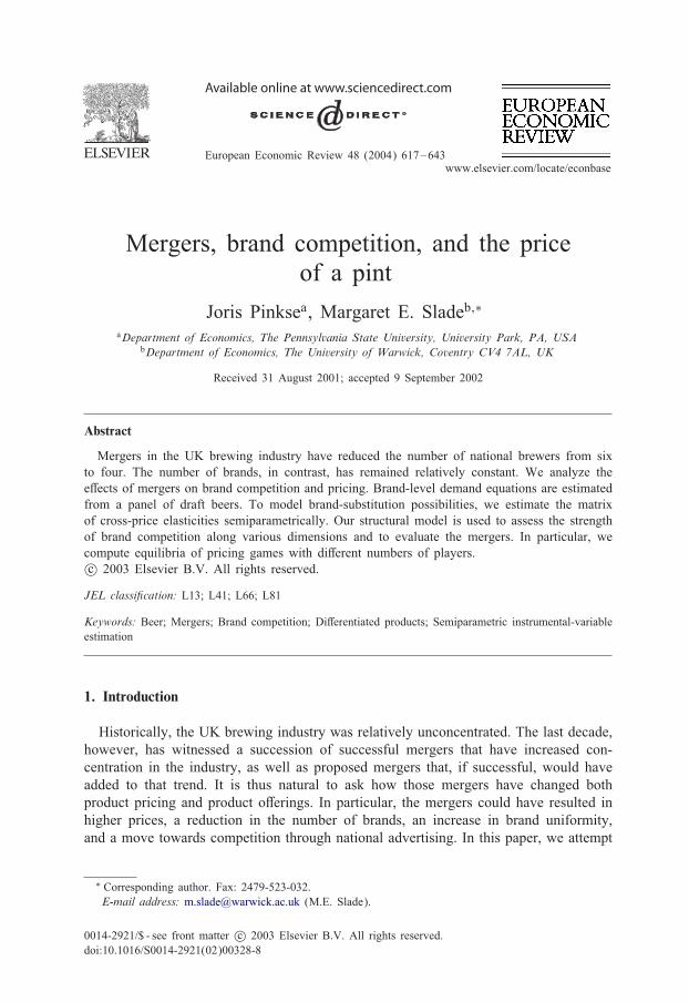
The elements of the exogenous common-boundary matrix, WCBX, are dummy vari-ables that equal one if i and j share an exogenous-market boundary but are not nearestneighbors, and zero otherwise, where i’s exogenous market consists of the set of con-sumers who are at least as close in Euclidean distance to i as to any other brand.The boundary between markets i and j thus consists of customers who are equidistantfrom the two. The endogenous common-boundary measure, WCBN, is similar exceptthat with this measure, boundaries are determined by relationships of equality of utilitylosses. 28 Fig. 1 depicts endogenous market areas for London in the Drst time period.We also constructed variables NCBX (NCBN) to equal the number of exogenous

(endogenous) common-boundary neighbors for each brand. On average, brands have 7common-boundary neighbors.Matrices corresponding to each discrete metric were normalized so that the elements

of each row sum to one. This normalization was performed so that when the pricevector is multiplied by a matrix, the ith element of the resulting vector is the averageprice of, for example, rival beers that are of the same type of product as i.

7. The econometric estimates

7.1. Parametric estimates

Table 2 summarizes the IV estimates of demand. Table 2A is divided into threesections: the Drst is the intercept term, ai, whereas the second is the own-price term,bii. Both of these are functions of the characteristic vector, Xi. The characteristics in bii,however, have been interacted with price. The third section is the rival-price term bij,which is a function of the distance measures, dij. Variables in this section are weightedaverages of rival prices and are denoted RPW, where W is one of the distance matrices.To conserve space, the estimated coeHcients of the characteristic variables are not

shown. Instead, the Drst row in Table 2A indicates their signs, whereas subsequentrows indicate their signiDcance. Furthermore, each equation in this table contains atmost one distance measure. Finally, since brewer and product-type Dxed e4ects werenever signiDcant, the equations that are shown do not include Dxed e4ects.

28 This measure of closeness is very similar to the one used by Feenstra and Levinsohn (1995).


coverage

alco

ho

l

20 40 60

3.0

3.5

4.0

4.5

5.0

Fig. 1. Endogenous market areas for London.

In theory, all characteristics that are included in Xi could enter both ai and bii. Inpractice, however, each characteristic is highly correlated with the interaction of thatcharacteristic with price. For this reason, the variables that appear in ai and those thatappear in bii are never the same. We have tried to allocate the variables in what wethink is a sensible fashion. Nevertheless, the allocation is somewhat arbitrary. 29 Inaddition, since coverage was found to be an important determinant of a brand’s marketsize and own-price elasticity, we have included coverage in both parts of the table.Di4erent functional forms were used to avoid collinearity, with LCOV = log(COV)and COVR = 1=COV.First consider the intercepts, ai. In all speciDcations, high coverage is associated with

high sales. In addition, sales are higher in independent establishments and in London.Finally, a high alcohol content has a positive but weak e4ect on sales. None of theseresults is surprising.

29 We experimented with other speciDcations and found that our principal conclusions were not a4ected.


Table 2IV demand equations

A: Equations with a single distance measure

Intercept Own price Rival price(ai) (bii) (bij)

CONS LCOV ALC PUBM PER1 REG1 PRICE PRCOVR PRPREM PRNCBX VAR. COEF. t STAT

− + + − + + − + − −∗∗∗ ∗∗∗ ∗ ∗∗∗ ∗∗∗ ∗ ∗∗∗ ∗∗ ∗ None∗∗∗ ∗∗∗ ∗ ∗∗ ∗∗∗ ∗∗∗ ∗∗∗ ∗ RPPROD 0.82 2.6

∗∗∗ ∗ ∗∗∗ ∗∗∗ ∗∗∗ ∗∗ ∗ RPBREW −0:40 −1:1∗∗∗ ∗∗∗ ∗∗∗ ∗∗∗ ∗ ∗∗∗ ∗ RPALC 0.16 0.7

∗∗∗ ∗∗∗ RPCOV −1:38 −1:7∗∗∗ ∗∗∗ ∗∗∗ ∗∗∗ ∗∗∗ ∗∗ ∗ RPCBN 0.04 0.7∗∗∗ ∗∗∗ ∗∗ ∗∗∗ ∗∗∗ ∗∗ ∗∗∗ ∗∗ ∗ RPCBX −0:08 −1:7∗∗∗ ∗∗∗ ∗∗∗ ∗∗∗ ∗∗∗ ∗∗ ∗ RPNNN 0.06 1.2∗∗∗ ∗∗∗ ∗ ∗∗∗ ∗∗∗ ∗ ∗∗∗ ∗∗ ∗ RPNNX 0.008 0.2

Semiparametric estimates with RPPROD∗∗∗ ∗∗∗ ∗∗ ∗∗∗ ∗∗∗ ∗∗ 3 expansion terms∗∗∗ ∗∗∗ ∗ ∗∗∗ ∗∗∗ ∗∗∗ 5 expansion terms

B: IV Equation with multiple distance measures

RPPROD RPBREW RPALC RPCBN RPNNN

0.82 −0:19 0.16 0.02 0.05(2.5) (−0:5) (1.2) (0.3) (0.9)

C: IV Equation used in evaluation of games

Intercept Own price Rival price(ai) (bii) (bij)

CONS LCOV ALC PUBM PER1 REGL PRICE PRCOVR PRPREM PRNCBX RPPROD RPALC

−159:1 60.3 8.80 −11:0 3.81 31.5 −1:13 0.17 −0:03 −0:12 0.71 0.22(−4:0) (11.7) (0.7) (−1:9) (0.8) (6.4) (−2:9) (7.8) (−0:1) (−2:7) (2.6) (1.6)

Standard errors corrected for heteroskedasticity and spatial correlation of unknown form. t statistics inparentheses.

∗Denotes signiDcance at 10%.∗∗Denotes signiDcance at 5%.∗∗∗Denotes signiDcance at 1%.

Next consider the own-price e4ects, bii. Premium and popular brands have steeper(i.e., more negative) slopes (recall that COVR is an inverse measure of coverage).In addition, when a brand has a large number of neighbors, its sales are more pricesensitive.More important and the focus of the paper are the determinants of brand substi-

tutability. The table shows that the most signiDcant measure of rivalry is RPPROD,


which implies that competition is strongest among brands that are of the same producttype. Indeed, none of the other measures of substitution is signiDcantly di4erent from0 at the 5% level.Table 2B shows a speciDcation with multiple distance measures. As before, the

discrete measure same-product-type has the highest explanatory power. In additionbeers with similar alcohol contents tend to compete, but this e4ect is weaker.Table 2C shows the Dnal parametric speciDcation. Only the same-product-type and

similar-alcohol-content measures, RPPROD and RPALC, are included in this speci-Dcation. This demand equation is thus similar to a nested logit, where the nests areproduct types. In addition to the product groupings, however, beers with similar alcoholcontents compete, regardless of type.

7.2. Semiparametric estimates

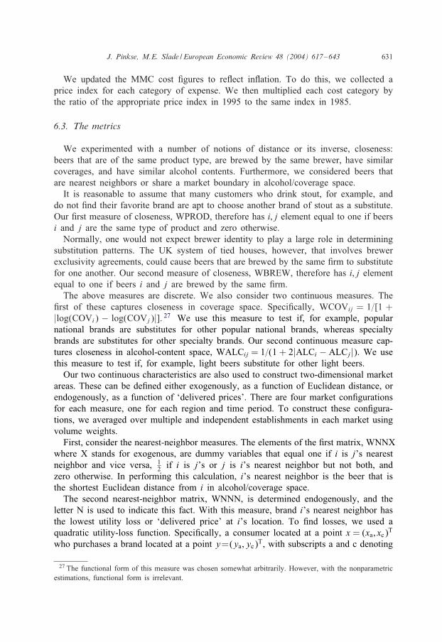
We have carried out experiments in which g is an unspeciDed function of the distancebetween brands in alcohol and/or coverage space and several discrete brand-similaritymeasures. The results are not qualitatively di4erent from the fully parametric case, andhence we present only one speciDcation. This one is identical to the second equation inTable 2A, except that the same-product-type distance measure, WPROD, is interactedwith terms of a Fourier-series expansion of di4erence in alcohol contents, WALC. Wereport speciDcations with three and Dve expansion terms, which can be found in thebottom portion of Table 2A. The table shows that the semiparametric estimates areidentical in sign and similar in signiDcance to the parametric ones. However, since thenumber of regressors is greater in a semiparametric speciDcation, standard errors tendto be larger.The estimate of the function g for the speciDcation with Dve expansion terms is

shown in Fig. 2. The graph shows how competition between brands that are of thesame product type varies as the di4erence in their alcohol contents increases. In additionwe show 5% and 2.5% asymptotic one-sided pointwise (Bonferroni) conDdence bands.Those bands have been corrected for spatial correlation, which makes them widerthan without such a correction. At a 5% level of signiDcance, we conclude that thecross-price elasticities are nonzero. However, we cannot reject the hypothesis that g isconstant.Given that g is an approximately linear function of the distance measures, which

means that our IV estimates are consistent, we use the equation that appears in Table2C for validity checks and merger evaluation.

8. Model assessment and use

We assess our model of demand, cost, and market equilibrium in three ways: weexamine the implied own and cross-price elasticities and compare them to previouselasticity estimates for beer, we test if our equilibrium assumption is consistent withobserved margins, and we compare observed and predicted prices under the ownershipstructure that prevailed when the data were collected.


Alcohol distance

effe

ct

0.0 0.5 1.0 1.5 2.0

0.0

0.5

1.0 g5% confidence band2.5% confidence band

Fig. 2. g, Same product type rivals (5 expansion terms).

First, however, we assessed identiDcation and checked regularity conditions. Withrespect to identiDcation, we used our test of correlation between the residuals andvarious groups of instruments. This process revealed no evidence of endogeneity. Forexample, when we examined price in the other region by itself, the p-value for the testwas 0.20, and when we examined the price instruments as a group, the p-value was0.38. We also estimated the demand equation with each set of instruments separately,as well as with both sets together, and found that our estimated elasticities were notvery sensitive to that choice. 30

With respect to curvature, all of the eigenvalues of the estimated matrix B, which isthe negative of the Hessian of the indirect-utility function, are negative at the mean ofthe data. This must be the case if B is negative deDnite and shows a close adherenceto quasi-convexity of the indirect-utility function.

8.1. Own and cross-price elasticities

There are many previous estimates of the industry own-price elasticity of demand forbeer, which is the percentage change in total beer consumption due to a 1% increase

30 The equations that we report were estimated with both sets of instruments.


Table 3Own and cross-price elasticities for selected brands (London) evaluated at observed prices and quantities

Brand Tennants Stella Lowenbrau Toby Websters Courage Greene GuinessPilsner Artois Bitter Yorks Bitter Best King IPA

Alcohol content 3.2% 5.2% 5.0% 3.3% 3.5% 4.0% 3.6% 4.1%product type Reg. Lager Prem. Lager Prem. Lager Keg Ale Keg Ale Real Ale Real Ale StoutNo. of neighbors 12 8 8 12 8 15 9 2

Tennents Pilsner −4:80 0.189 0.181 0.021 0.018 0.011 0.013 0.012Stella Artois 0.068 −2:49 0.085 0.002 0.003 0.004 0.003 0.005Lowenbrau 0.091 0.119 −3:10 0.003 0.004 0.006 0.004 0.007Toby Bitter 0.030 0.009 0.009 −4:87 0.457 0.015 0.018 0.016Websters Bitter 0.013 0.006 0.006 0.227 −3:20 0.010 0.013 0.010Courage Best 0.009 0.007 0.008 0.010 0.011 −2:79 0.124 0.021Greene King IPA 0.064 0.038 0.041 0.061 0.090 0.852 −12:62 0.081Guiness 0.002 0.002 0.002 0.001 0.002 0.004 0.002 −0:93

in the prices of all brands. Our estimated industry own-price elasticity is −0:5, whichis in line with previous estimates. 31

Estimated own-price elasticities for individual brands, which are calculated holdingthe prices of rival brands constant, are much rarer. Our average brand own-price elas-ticity is −4:6, which is in line with estimates obtained by Hausman et al. (1994). Theirbrand own-price elasticities average −5:0.One can deDne a total cross-price elasticity, which is the percentage change in one

brand’s sales due to a 1% increase in the prices of all of its rivals. We Dnd that thiselasticity averages 4.1. Partial cross-price elasticities, which are percentage changesin one brand’s sales due to a 1% increase in the price of a single rival, vary bybrand pair. Moreover, as there are many brands, partial cross-price elasticities mustbe small. Indeed, since our cross-price elasticities are nonnegative (i.e., the brands aresubstitutes), stability requires that, on average, their sum be less than the absolute valueof the own-price elasticities.It is not practical to examine 63 own and approximately 4,000 cross-price elastic-

ities. Table 3 therefore contains elasticities for a selected subsample of brands soldin London. This subsample contains one regular lager, Tennants Pilsner, two premiumlagers, Stella Artois and Lowenbrau, two keg ales, Toby and Websters Yorks Bitter,two real ales, and one stout. One of the real ales, Courage Best, is a best-selling brandbrewed by a national brewer, whereas the other, Greene King IPA, is a small-salesbrand brewed by a regional brewer. Finally, the stout, Guiness, is an outlier with acoverage that is substantially higher than that of any other brand. In addition to iden-tifying the type of each brand, the Drst row of the table shows the brand’s alcoholcontent and the number of its exogenous common-boundary neighbors.

31 For example, Clements and Johnson (1983), Johnson et al. (1992), Lee and Tremblay (1992), Hogartyand Elzinga (1972) and Hausman et al. (1994) estimate industry own-price elasticities for beer to be −0:1,−0:3, −0:6, −0:9, and −1:6, respectively.


Table 4Nash-equilibrium prices (London)

Actual Status quo Before %/ After %/

Mean 167.8 168.4 167.4 −0:6 173.5 +3:0Standard deviation 20.2 29.5 22.1 30.2

Table 3 shows that there is substantial variation in brand own-price elasticities. Fur-thermore, most of the magnitudes are plausible. In particular, if one ranks the recipro-cals of the absolute values of the own-price elasticities and ranks the price/cost margins,the rankings are very similar. The table also shows that, as expected, cross-price elas-ticities are greater when brands are of the same type and have similar alcohol contents.All brand own-price elasticities are signiDcant at 1%. Cross-price elasticities for

brands of the same type are also signiDcant at 1%. When brands are of di4erent types,however, their cross-price elasticities are not signiDcant at 5% but are at 10%.

8.2. Comparing status quo margins and prices

We can use our estimates of demand and cost to test our equilibrium assumption. Inparticular, we wish to determine if a static game in prices is a reasonable description ofinteractions in the market. To do this, we construct excess margins, !�i, for the statusquo game � and test if they are on average zero, where the status quo ownershipconDguration is the situation that prevailed when the data were collected. In otherwords, with the status quo, there are ten brewers, four nationals, Bass, Carlsberg–Tetley, Scottish Courage, and Whitbread, two brewers without tied estate, and fourregionals.The mean excess margin is −0:009, the median is −0:024, and the range is −0:30

to 0.56. Furthermore, the t statistic for the hypothesis that 1=n�i!�i = 0 is −0:66,which means that, on average, predicted and observed margins are equal and Bertrandbehavior cannot be rejected. 32

On average, excess margins are zero. Nevertheless, there are systematic deviationsfrom zero in the estimates. In particular, more popular and higher-strength brands, aswell as those that are sold in multiple establishments, are less competitively priced.Next consider prices. The Drst columns of Table 4 show observed and Nash-

equilibrium (NE) prices calculated under the status quo assumption for London. Theaverage predicted price is 168.4, slightly higher than the observed average of 167.8,and the standard deviation is 29.5, compared to 20.2. Status quo prices are thus ap-proximately centered around the true value but are more variable. However, as with

32 The test is based on the fact that any sequence of i.i.d. variates with uniformly bounded momentsgreater than two, whether they are estimators or not, have a limiting normal distribution; this follows fromthe Lindeberg theorem, e.g. Doob (1953, Theorem 4.2). The notion that the estimators !�i are independent,even in the limit, is debatable. If they are dependent however, the t-statistics would generally be smaller.


0

1

2

3

4

5

6

7

8

89 90 91 92 93 94 95 96 97 98

Year

Per

cen

tag

e

Observed Changes Predicted Changes

Fig. 3. Observed and predicted real retail price changes.

excess margins, there are systematic deviations between observed and predicted prices.Nevertheless, we feel that, on average, the model predicts well.

8.3. The price e>ects of the mergers

Given that our estimated model of demand is well behaved and that our equilibriumassumption is not rejected, we can use our model for a formal analysis of the impactsof mergers and divestitures. This analysis involves solution of market games underdi4erent assumptions about ownership.Static NE prices are calculated under three scenarios: before, status quo, and after.

The before scenario is created by undoing the Scottish Courage merger. With thisscenario, there are Dve national brewers, and the prices of the brands that belonged toCourage before the merger are chosen by one player, whereas the prices of the brandsthat belonged to S&N are chosen by another. The after scenario is created by allowingthe Bass/Carlsberg–Tetley merger to occur. With this scenario, there are three nationalbrewers, and the prices of all Bass and Carlsberg–Tetley brands are chosen by a singleplayer. With all three scenarios, the structure of the rest of the industry is unchanged.Equilibrium prices under the various scenarios are summarized in Table 4. For con-

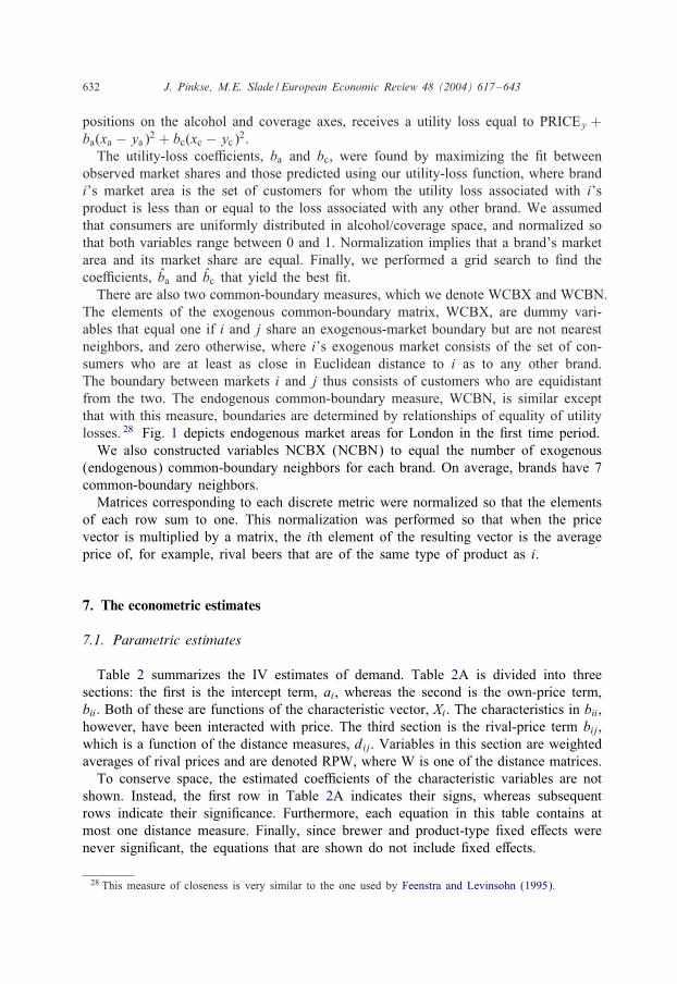
sistency, before and after prices are compared to status quo, rather than to observedprices. The table shows that undoing the Scottish Courage merger would have littlee4ect on prices. Indeed, the price decline is less than one percent. A merger betweenBass and Carlsberg–Tetley, in contrast, is predicted to result in an overall price increaseof 3%. To us, this number seems substantial.Fig. 3 shows observed and predicted price changes. One can see that the observed

and predicted changes in the year of the Scottish Courage merger are close to one


another. In addition, the change that is predicted to accompany the BCT merger issubstantially larger than the change that occurred absent the merger. 33

Why might a merger between S&N and Courage not cause substantial price in-creases? The answer lies in both the geographic and the brand Dt. Geographically,S&N had most of its market in the north, whereas Courage was a southern beer. InLondon, therefore, Courage dominated S&N, and the local di4erence in their marketshares was greater than the national di4erence. Moreover, Courage had a strong posi-tion in lagers, with best selling Fosters and Kronenbourg. S&N, in contrast, had onlyBecks, which was not a heavy seller. Comparing ales, both Courage Best and JohnSmiths were big brands for Courage, whereas S&N’s biggest seller, Theakstons, had amuch smaller share of the London market.The brand overlap between Bass and Carlsberg–Tetley, in contrast, was more sub-

stantial, particularly in lagers. Indeed, both had best-selling lagers, Carling for Bassand Carlsberg for Carlsberg–Tetley, as well as several other very popular brands. Ge-ographically, the Drms originated in the north (Tetley) or north central (Bass) part ofthe country. Their geographic strengths were thus more similar than those of Courageand S&N, which meant that their local and national market shares were closer.The geographic and brand overlap (or lack thereof) is undoubtedly responsible for

the di4erent impacts that the mergers are predicted to have on prices. Indeed, thedi4erence in market shares, 37% for Scottish Courage versus 34% for BCT in thegeographic and brand market studied, is small. Moreover, if one were to considerlocal-market shares alone, one would expect the Scottish Courage merger to be moreanticompetitive, which is the opposite of what we Dnd.

9. Other consequences of the mergers

Mergers can a4ect all aspects of a Drm’s business, not just prices. We thereforeexamine the possible ramiDcations for brand selection and productive eHciency infor-mally.Although, in general, there is considerable brand churn, very little of it concerns

products than constitute as much as 12% of local markets. Moreover, it is clear frominterviews with industry managers and marketers that Drms are principally interestedin the fate of their best-selling brands. None of these disappeared during the ten-yearperiod. Furthermore, according to people in the industry, the brands that did disappearwould have done so absent the merger, albeit at a possibly di4erent rate.In contrast to brand disappearance, new best-selling brands were introduced. These

fall into two classes: foreign-owned lagers and hybrid ales. The lagers that are in thesample but were not sold in the UK in 1985 are Grolsch, a Dutch beer, and Coors, anAmerican beer. It is highly unlikely, however, that absent the mergers (or in the caseof BCT, had the merger occurred) those brands would not have entered the market.

33 The large price increases that occurred in the beginning of the decade are perhaps due to forced salesof retail outlets (see Slade, 1998).


Hybrid ales are a relatively recent addition to the UK market. A hybrid is a keg alethat uses a nitrogen and carbon-dioxide mix in dispensing that causes it to be smootherand to more closely resemble a cask ale. After Bass introduced Ca4reys, which is themost popular hybrid ale, other brewers followed suit. As with the lagers, it is highlyunlikely that the introduction of hybrid ales would have been retarded or aborted bymergers or divestitures.The two mergers under consideration are thus unlikely to have had much of an

impact on product selection. However, they could have caused promotional e4orts tobe concentrated on a smaller number of best-selling brands. If true, there might havebeen less variety in consumption if not in o4erings.When a merger occurs it is usually accompanied by restructuring and cost reduction.

Indeed, increased eHciency is one reason why Drms undertake mergers. It is thereforepossible that cost reductions could have o4set market-power increases, and the mergerscould have caused prices to fall.The BCT merger, like other mergers in the brewing industry, was forecast to re-

sult in cost savings of two types: brewery closings and savings in distribution andwholesaling costs. Retail costs were not supposed to be a4ected. In the absence of themerger, however, the breweries that were scheduled to close have in fact closed. Incontrast, there has been little reduction in distribution and sales forces. If there aremerger-speciDc o4setting cost savings, we must therefore look for them in a reductionin wholesaling costs, and, according to the MMC’s cost estimates, wholesaling costsconstitute only 10% of the retail price of beer.It is possible to assess whether cost reductions could have o4set increased market

power formally. To do this, we solved for the cost reduction that would be requiredto insure that, in equilibrium and on average, no price increase would occur. In per-forming this exercise, we recognized that only the costs of the merging Drms would bereduced. 34 We found that the costs of the merging Drms would have to fall by about20% to just o4set the increase in market power. Given that wholesaling costs are only10% of price, a reduction of the required magnitude would not have been possible.Finally, entry is unlikely to mitigate the e4ects of mergers. The number of brewers

has been in decline for decades, and no Drms have entered the national segment of theindustry. Indeed, there were six national brewers in 1960, each of which is roughlyidentiDable with one of the six that existed in 1990, just prior to the Courage/GrandMet merger.

10. Conclusions

Our analysis of brand substitution in UK markets for draft beer indicates that com-petition is relatively local. In particular, we Dnd that brands that are the of the sameproduct type compete most vigorously. Our model of demand is thus similar to a nestedlogit. Competition among groups of products, however, is not a maintained assumption,

34 SpeciDcally, we substituted ci = (1 − �) × ci if i was a BCT brand, and ci = ci if not, into the afterDrst-order conditions, and we solved for the value of � that would leave prices unchanged on average.


since this possibility is encompassed in a broader model of substitution. We also Dndthat beers with similar alcohol contents compete regardless of type, but the strength ofthis competition is considerably weaker.When we use our estimated demands and costs to analyze the game that the brewers

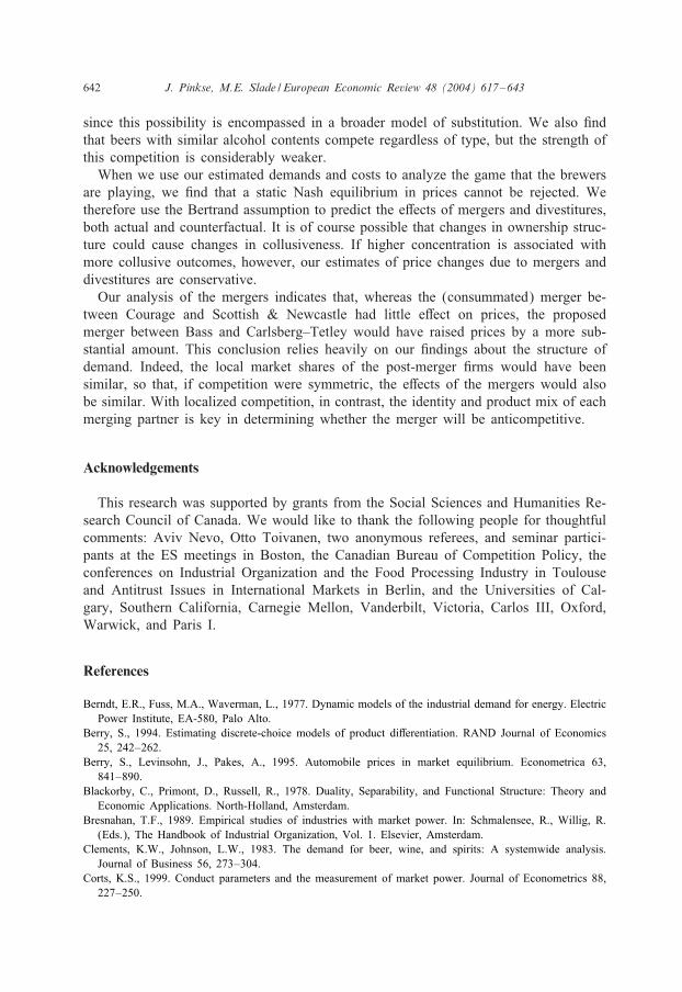
are playing, we Dnd that a static Nash equilibrium in prices cannot be rejected. Wetherefore use the Bertrand assumption to predict the e4ects of mergers and divestitures,both actual and counterfactual. It is of course possible that changes in ownership struc-ture could cause changes in collusiveness. If higher concentration is associated withmore collusive outcomes, however, our estimates of price changes due to mergers anddivestitures are conservative.Our analysis of the mergers indicates that, whereas the (consummated) merger be-

tween Courage and Scottish & Newcastle had little e4ect on prices, the proposedmerger between Bass and Carlsberg–Tetley would have raised prices by a more sub-stantial amount. This conclusion relies heavily on our Dndings about the structure ofdemand. Indeed, the local market shares of the post-merger Drms would have beensimilar, so that, if competition were symmetric, the e4ects of the mergers would alsobe similar. With localized competition, in contrast, the identity and product mix of eachmerging partner is key in determining whether the merger will be anticompetitive.

Acknowledgements

This research was supported by grants from the Social Sciences and Humanities Re-search Council of Canada. We would like to thank the following people for thoughtfulcomments: Aviv Nevo, Otto Toivanen, two anonymous referees, and seminar partici-pants at the ES meetings in Boston, the Canadian Bureau of Competition Policy, theconferences on Industrial Organization and the Food Processing Industry in Toulouseand Antitrust Issues in International Markets in Berlin, and the Universities of Cal-gary, Southern California, Carnegie Mellon, Vanderbilt, Victoria, Carlos III, Oxford,Warwick, and Paris I.

References

Berndt, E.R., Fuss, M.A., Waverman, L., 1977. Dynamic models of the industrial demand for energy. ElectricPower Institute, EA-580, Palo Alto.

Berry, S., 1994. Estimating discrete-choice models of product di4erentiation. RAND Journal of Economics25, 242–262.

Berry, S., Levinsohn, J., Pakes, A., 1995. Automobile prices in market equilibrium. Econometrica 63,841–890.

Blackorby, C., Primont, D., Russell, R., 1978. Duality, Separability, and Functional Structure: Theory andEconomic Applications. North-Holland, Amsterdam.

Bresnahan, T.F., 1989. Empirical studies of industries with market power. In: Schmalensee, R., Willig, R.(Eds.), The Handbook of Industrial Organization, Vol. 1. Elsevier, Amsterdam.

Clements, K.W., Johnson, L.W., 1983. The demand for beer, wine, and spirits: A systemwide analysis.Journal of Business 56, 273–304.

Corts, K.S., 1999. Conduct parameters and the measurement of market power. Journal of Econometrics 88,227–250.


Deaton, A., Muellbauer, J., 1980. An almost ideal demand system. American Economic Review 70,312–326.

Diewert, W.E., 1971. An application of the shephard duality theorem: A generalized Leontief productionfunction. Journal of Political Economy 79, 481–507.

Doob, J.L., 1953. Stochastic Processes. Wiley, New York.Feenstra, R.C., Levinsohn, J.A., 1995. Estimating markups and market conduct with multidimensional productattributes. Review of Economic Studies 62, 19–52.

Gorman, W.M., 1971. Two-stage budgeting. Mimeo.Hausman, J., Leonard, G., Zona, D., 1994. Competitive analysis with di4erentiated products. Annalesd’Econometrie et de Statistique 34, 159–180.

Hogarty, T.F., Elzinga, K.G., 1972. The demand for beer. Review of Economics and Statistics 54, 196–198.Ivaldi, M., Verboven, F., 2000. Quantifying the e4ects from horizontal mergers: The European heavy trucksmarket. Mimeo.

Johnson, J.A., Oksanen, E.H., Veall, M.R., Fretz, D., 1992. Short-run and long-run elasticities for Canadianconsumption of alcoholic beverages: An error-correction mechanism/cointegration approach. Review ofEconomics and Statistics 74, 64–74.

Lee, B., Tremblay, V.J., 1992. Advertising and the market demand for beer. Applied Economics 24, 69–76.McFadden, D., 1974. Conditional logit analysis of qualitative choice behavior. In: Zarembka, P. (Ed.),Frontiers in Econometrics. Academic Press, New York, pp. 105–142.

McFadden, D., 1978a. Modeling the choice of residential location. In: Karlqvist, A., et al. (Ed.), SpatialInteraction Theory and Planning Models. North-Holland, Amsterdam.

McFadden, D., 1978b. The general linear proDt function. In: Fuss, M., McFadden, D. (Eds.), ProductionEconomics: A Dual Approach to Theory and Applications, Vol. 1. North-Holland, Amsterdam,pp. 269–286.

McFadden, D., Train, K., 2000. Mixed MNL models for discrete response. Journal of Applied Econometrics15, 447–470.

Monopolies and Mergers Commission (MMC), 1989. The Supply of Beer. Her Majesty’s Stationary OHce,London.

Nevo, A., 2000. Mergers with di4erentiated products: The case of the ready-to-eat cereal industry. RANDJournal of Economics 31, 395–421.

Newey, W.K., West, K.D., 1987. A simple positive semi-deDnite, heteroskedasticity and autocorrelationconsistent covariance matrix estimator. Econometrica 55, 703–708.

Petrin, E., 2002. Quantifying the beneDts of new products: The case of the minivan. Journal of PoliticalEconomy 110, 705–729.

Pinkse, J., Slade, M.E., Brett, C., 2002. Spatial price competition: A semiparametric approach. Econometrica70, 1111–1153.

Slade, M.E., 1998. Beer and the tie: Did divestiture of Brewer-owned public houses lead to higher beerprices? Economic Journal 108, 565–602.

Slade, M.E., 2002. Market power and joint dominance in the UK brewing industry. Mimeo., University ofWarwick.

Werden, G.J., Froeb, L.M., 1994. The e4ects of mergers in di4erentiated products industries: Logit demandand merger policy. Journal of Law, Economics, and Organization 10, 407–426.

Documents

Mergers,brandcompetition,andtheprice ofapint online at EuropeanEconomicReview48(2004)617–643 Mergers,brandcompetition,andtheprice ofapint JorisPinksea,MargaretE.Sladeb;∗ aDepartmentofEconomics