Mercury's moment of inertia from spin and gravity data

Mercury’s moment of inertia from spin and gravity data

Jean-Luc Margot,1,2 Stanton J. Peale,3 Sean C. Solomon,4,5 Steven A. Hauck II,6

Frank D. Ghigo,7 Raymond F. Jurgens,8 Marie Yseboodt,9 Jon D. Giorgini,8

Sebastiano Padovan,1 and Donald B. Campbell10

Received 15 June 2012; revised 31 August 2012; accepted 5 September 2012; published 27 October 2012.

[1] Earth-based radar observations of the spin state of Mercury at 35 epochs between 2002and 2012 reveal that its spin axis is tilted by (2.04 � 0.08) arc min with respect to the orbitnormal. The direction of the tilt suggests that Mercury is in or near a Cassini state.Observed rotation rate variations clearly exhibit an 88-day libration pattern which is due tosolar gravitational torques acting on the asymmetrically shaped planet. The amplitude ofthe forced libration, (38.5 � 1.6) arc sec, corresponds to a longitudinal displacementof �450 m at the equator. Combining these measurements of the spin properties withsecond-degree gravitational harmonics (Smith et al., 2012) provides an estimate of thepolar moment of inertia of Mercury C/MR2 = 0.346 � 0.014, whereM and R are Mercury’smass and radius. The fraction of the moment that corresponds to the outer librating shell,which can be used to estimate the size of the core, is Cm/C = 0.431 � 0.025.

Citation: Margot, J.-L., S. J. Peale, S. C. Solomon, S. A. Hauck II, F. D. Ghigo, R. F. Jurgens, M. Yseboodt, J. D. Giorgini,S. Padovan, and D. B. Campbell (2012), Mercury’s moment of inertia from spin and gravity data, J. Geophys. Res., 117, E00L09,doi:10.1029/2012JE004161.

1. Introduction

[2] Bulk mass density r = M/V is the primary indicator ofthe interior composition of a planetary body of mass M andvolume V. To quantify the structure of the interior, the mostuseful quantity is the polar moment of inertia

C ¼ZVr x; y; zð Þ x2 þ y2

� �dV : ð1Þ

In this volume integral expressed in a cartesian coordinatesystem with principal axes {x, y, z}, the local density ismultiplied by the square of the distance to the axis of rotation,which is assumed to be aligned with the z axis. Moments of

inertia computed about the equatorial axes x and y aredenoted by A and B, with A < B < C. The moment of inertia(MoI) of a sphere of uniform density and radius R is 0.4MR2.Earth’s polar MoI value is 0.3307 MR2 [Yoder, 1995],indicating a concentration of denser material toward thecenter, which is recognized on the basis of seismological andgeochemical evidence to be a primarily iron-nickel coreextending �55% of the planetary radius. The value for Marsis 0.3644 MR2, suggesting a core radius of �50% of theplanetary radius [Konopliv et al., 2011]. The value for Venushas never been measured. Here we describe our determina-tion of the MoI of Mercury and that of its outer rigid shell(Cm), both of which can be used to constrain models of theinterior [Hauck et al., 2007; Riner et al., 2008; Rivoldiniet al., 2009].[3] Both the Earth andMars polar MoI values were secured

by combining measurements of the precession of the spinaxis due to external torques (Sun and/or Moon), whichdepends on [C � (A + B)/2]/C, and of the second-degreeharmonic coefficient of the gravity field C20 = � [C �(A + B)/2]/(MR2). Although this technique is not applicable atMercury, Peale [1976] proposed an ingenious procedure toestimate the MoI of Mercury and that of its core based ononly four quantities. The two quantities related to the gravityfield, C20 and C22 = (B � A)/(4MR2), have been determinedto better than 1% precision by tracking of the MESSENGERspacecraft [Smith et al., 2012]. The two quantities related tothe spin state are the obliquity q (tilt of the spin axis withrespect to the orbit normal) and amplitude of forced librationin longitude g (small oscillation in the orientation of the longaxis of Mercury relative to uniform spin). They have beenmeasured by Earth-based radar observations at 18 epochsbetween 2002 and 2006. These data provided strong obser-vational evidence that the core of Mercury is molten, and that

1Department of Earth and Space Sciences, University of California, LosAngeles, California, USA.

2Department of Physics and Astronomy, University of California, LosAngeles, California, USA.

3Department of Physics, University of California, Santa Barbara,California, USA.

4Department of Terrestrial Magnetism, Carnegie Institution ofWashington, Washington, D. C., USA.

5Lamont-Doherty Earth Observatory, Columbia University, Palisades,New York, USA.

6Department of Earth, Environmental, and Planetary Sciences, CaseWestern Reserve University, Cleveland, Ohio, USA.

7National Radio Astronomy Laboratory, Green Bank, West Virginia,USA.

8Jet Propulsion Laboratory, Pasadena, California, USA.9Royal Observatory of Belgium, Uccle, Belgium.10Department of Astronomy, Cornell University, Ithaca, New York, USA.

Corresponding author: J.-L. Margot, Department of Earth and SpaceSciences, University of California, 595 Charles Young Dr. E., Los Angeles,CA 90095, USA. ( [email protected])

©2012. American Geophysical Union. All Rights Reserved.0148-0227/12/2012JE004161

JOURNAL OF GEOPHYSICAL RESEARCH, VOL. 117, E00L09, doi:10.1029/2012JE004161, 2012

E00L09 1 of 11

Mercury occupies Cassini state 1 [Margot et al., 2007]. Herewe extend the baseline of observations to a total of 35 epochsspanning 2002–2012, and we provide improved estimates ofq, g, C, and Cm.

2. Methods

2.1. Formalism

[4] Peale [1969, 1988] has shown that a simple relation-ship exists between obliquity, gravity harmonics, and C/MR2

for bodies in Cassini state 1:

K1 qð ÞC20MR2

C

� �þ K2 qð Þ4C22

MR2

C

� �¼ K3 qð Þ; ð2Þ

where the functions K1,2,3 depend only on obliquity andknown ancillary quantities (orbital inclination and precessionrate with respect to the Laplace pole). Equation (2) or one ofits explicit variants can be used to determine Mercury’s MoIC/MR2 if the obliquity q and gravity coefficients C20 and C22

are known. By far the largest source of uncertainty in esti-mating the MoI comes from measurements of the obliquity q.Errors on the determination of ancillary quantities contributeto the uncertainty at the percent level [Yseboodt and Margot,2006]. Residual uncertainties in the knowledge of the gravityharmonics [Smith et al., 2012] contribute at less than thepercent level.[5] Peale [1976, 1988] also showed that observations of

the forced libration in longitude, which results from torquesby the Sun on the asymmetric figure of the planet, caninform us about the MoI of the outer rigid shell Cm (or,equivalently, that of the core Cc = C � Cm). This is becausethe magnitude of the torque and the amplitude of the libra-tion are both proportional to (B � A)/Cm. The MoI of theouter rigid shell is obtained by writing the identity

Cm

C¼ 4C22

MR2

C

� �Cm

B� A

� �: ð3Þ

[6] The four quantities identified by Peale [1976] can beused to probe the interior structure of the planet. The

gravitational harmonics C20 and C22 are combined with theobliquity q in equation (2) to yield C/MR2. This also yields C,since M and R are known. The amplitude of the forcedlibration provides the quantity (B � A)/Cm, which is usedwith previous quantities in equation (3) to yieldCm/C. This inturn yields Cm and Cc. Models of the interior must satisfy theMoI values for the core (Cc) and for the entire planet (C).

2.2. Observational Technique

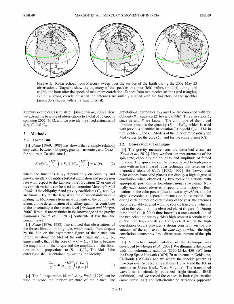
[7] The gravity measurements are described elsewhere[Smith et al., 2012]. Here we focus on measurements of thespin state, especially the obliquity and amplitude of forcedlibration. The spin state can be characterized to high preci-sion with an Earth-based radar technique that relies on thetheoretical ideas of Holin [1988, 1992]. He showed thatradar echoes from solid planets can display a high degree ofcorrelation when observed by two receiving stations withappropriate positions in four-dimensional space-time. Nor-mally each station observes a specific time history of fluc-tuations in the echo power (also known as speckles), and thesignals recorded at separate antennas do not correlate. Butduring certain times on certain days of the year, the antennasbecome suitably aligned with the speckle trajectory, which istied to the rotation of the observed planet (Figure 1). Duringthese brief (�10–20 s) time intervals a cross-correlation ofthe two echo time series yields a high score at a certain valueof the time lag (�5–10 s). The epoch at which the highcorrelation occurs provides a strong constraint on the ori-entation of the spin axis. The time lag at which the highcorrelation occurs provides a direct measurement of the spinrate.[8] A practical implementation of the technique was

developed by Margot et al. [2007]. We illuminate the planetwith monochromatic radiation (8560 MHz, 450 kW) fromthe Deep Space Network (DSN) 70 m antenna in Goldstone,California (DSS-14), and we record the speckle pattern asit sweeps over two receiving stations (DSS-14 and the 100 mantenna in Green Bank, West Virginia). The transmittedwaveform is circularly polarized (right-circular, IEEEdefinition), and we record the echoes in both right-circular(same sense, SC) and left-circular polarizations (opposite

Figure 1. Radar echoes from Mercury sweep over the surface of the Earth during the 2002 May 23observations. Diagrams show the trajectory of the speckles one hour (left) before, (middle) during, and(right) one hour after the epoch of maximum correlation. Echoes from two receive stations (red triangles)exhibit a strong correlation when the antennas are suitably aligned with the trajectory of the speckles(green dots shown with a 1 s time interval).

MARGOT ET AL.: MERCURY’S MOMENT OF INERTIA E00L09E00L09

2 of 11

sense, OC). To compensate for the Earth-Mercury Dopplershift, the transmitted waveform is continuously adjusted infrequency (by up to �2.5 MHz) so that the echo center at theGreen Bank Telescope (GBT) remains fixed at 8560 MHz.Because the Doppler is compensated for the GBT, there isa residual Doppler shift during reception at Goldstone.Differential Doppler corrections are performed by a pro-grammable local oscillator at the DSN so that the echocenter also remains fixed in frequency. We apply a numberof frequency downconversion, filtering, and amplificationoperations to the signal. During conversion to baseband thein-phase (I) and quadrature (Q) components of the signalare generated. Both are sampled at 5 MHz by our custom-built data-taking systems (http://www2.ess.ucla.edu/�jlm/research/pfs) and stored on a computer storage medium forsubsequent processing.

2.3. Data Reduction Technique

[9] After the observations we downsample our data toeffective sampling rates fs between 200 Hz and 5000 Hz andcompute the complex cross-correlation of the DSN and GBTsignals (Appendix A). This is a two-dimensional correlationfunction in the variables epoch t and time lag t. Examples ofone-dimensional slices through the peak of the correlationfunction are shown in Figure 1 of Margot et al. [2007]. Wefit Gaussians to the one-dimensional slices to obtain esti-mates of the epoch of correlation maximum t̂ and of the timelag t̂ that maximizes the correlation.[10] For epoch correlations, we typically use fs = 200 Hz,

about half the Doppler broadening due to Mercury’s rotation,and integration times of 1–2 s. The one-standard-deviationwidths of the Gaussians are used as nominal epoch uncer-tainties, with or without 1=

ffiffiffiffiffiffiffiffiffiffiSNR

pscaling, where SNR is

signal-to-noise ratio (Appendix A).[11] For time lag correlations, we typically use fs = 1000–

5000 Hz and integration times of 1 s, yielding �10–20independent estimates during the high correlation period.These estimates vary noticeably with time but display a highdegree of consistency, which allows us to remove obviousoutliers. We perform a linear regression on the remainingestimates and report the time lag t̂ corresponding to theepoch of correlation maximum t̂ . The root-mean squarescatter about the regression line is used as an estimate of thetime lag uncertainty.

2.4. Spin State Estimates

[12] The observables t̂ and t̂ are used to provide spin stateestimates (spin axis orientation and instantaneous spin rates).In these calculations the planet state vectors are furnished bythe Jet Propulsion Laboratory Planetary Ephemeris DE421[Folkner et al., 2008], and the Earth orientation is providedby the latest timing and polar motion data. The formalism forpredicting the (t, t) values that yield high correlations isdescribed in Appendix B. We link the observables t̂ and t̂ tospin state estimates using these predictions with the follow-ing procedures.[13] The space-time positions of the two receiving stations

at the epochs of correlation maxima are used to solve for thespin axis orientation that generates similar speckles at bothreceiving stations. We use a least-squares approach to min-imize the residuals between the predicted epochs and the

observed epochs. Various subsets of epoch measurementsare combined to identify the best-fit spin axis orientationreferred to the epoch J2000. The precession model for thespin axis is based on the assumption that the orbital preces-sion rates are applicable, which is expected if Mercuryclosely follows the Cassini state. The orbital precessionvalues are taken from Margot [2009] and amount to a pre-cession of �0.1 arc min over the 10-year observationinterval.[14] Once the spin axis orientation is determined, each

time lag measurement is used to determine the instantaneousspin rate at the corresponding epoch, once again based onthe similarity requirement for the speckles. We iterativelyadjust the nominal spin rate of 6.1385025 deg/day by amultiplicative factor until the predicted time lag matches theobserved time lag. A correction factor for refraction withinEarth’s atmosphere is applied to the spin rate at eachobservation epoch (Appendix C).[15] The nominal DSN-GBT baseline is 3,260 km in

length. In the spin rate problem, it is the projected baselinethat is relevant, i.e., the baseline component that is perpen-dicular to the line of sight. Because of the displacement of thelight rays due to refraction in the atmosphere, the effectiveprojected baseline differs from the nominal value. The worstcase correction at the largest zenith angle of� 84� is�150 mfor a projected baseline of�1200 km, i.e., a fractional changeof�1 part in 10,000. Because corrections are substantial onlyat very large zenith angles, the majority of our observationsare not affected significantly by atmospheric refraction.

3. Spin State

3.1. Observational Circumstances

[16] Between 2002 and 2012 we secured 58 sessions at theDSN and GBT telescopes (out of a larger number of sessionsrequested). Of those, 21 sessions were not successful. Thelost sessions at Goldstone were due to pointing problems (5),failure of the motor-generator (5), heat exchanger problems(2), a defective filament power supply (1), failure of thequasi-optical mirror (1), a defective data-taking system (1),sudden failure of the transmitter (1), and operator error (2).The lost tracks at GBT were due to repair work on the azi-muth track (2) and pointing (1). The remaining 37 sessionswere successful, but the data from two sessions near superiorconjunction are of low quality and were not used in theanalysis. Thus, data from 35 sessions obtained in a 10-yearinterval are presented in this paper, which roughly doublesthe number of sessions (18) and time span (4 years) of ourprevious analysis [Margot et al., 2007].[17] The observational circumstances of the 35 sessions

are listed in Table 1. The round-trip light time (RTT) toMercury strongly affects the SNR (∝RTT�4). The antennaelevation angles dictate the magnitude of the refractioncorrections. Refraction effects lengthen the effective dis-tance (the projected baseline) that the speckles travel duringthe measured time lag, which results in an increase in thespin rate that would have otherwise been determined. Therange of ecliptic longitudes of the projected baselines indi-cates that we have observed Mercury with a variety ofbaseline orientations, which is important for a secure deter-mination of the spin axis orientation.


3 of 11

3.2. Epoch and Time Lag Measurements

[18] The results of our epoch and time lag measurementsare shown in Table 2. Agreement between OC and SC valuesof the epochs of correlation maxima is generally excellent,with a root-mean square (RMS) deviation of 0.45 s. Thelargest discrepancy occurs for the 120314 data set with a 1.3 sdifference.[19] For the 100102 data set, reception of radar echoes

started while the high correlation condition was alreadyunderway, and we were not able to measure the peak of thecorrelation maximum. We were able to secure an instanta-neous spin rate estimate from repeated measurements duringthe second half of the high correlation period. Therefore, thisdata set was used for the determination of the instantaneousspin rate but not of the spin axis orientation.[20] For reasons that are not entirely understood, we

experienced considerable difficulties fitting for the epoch ofcorrelation maximum to the 090113 and 090114 data sets.Differences of up to 6 s in the correlation maximum wereobtained for various combinations of parameters (start timesand integration times), and we declared these data sets

unsuitable for epoch measurements. However, we were ableto use these data sets for time lag measurements.[21] We performed spin orientation fits that excluded the

120314 measurements because of the 1.3 s discrepancybetween OC and SC estimates of the epoch of correlationmaximum. Analysis suggests that the OC value (MJD56000.99151150) is inferior to the SC value (MJD56000.99149649): removing the OC data point typicallyimproves the goodness of fit by a factor of �3, whereasremoving the SC data point has no substantial effect on thereduced c2 value. Despite the preference for the SC value ofepoch t, we report the time lag measurement t at the OCepoch for consistency with all other runs, and because doingso has no impact on the spin rate fits.

3.3. Spin Axis Orientation

[22] The spin axis orientation fits indicate that we candetermine the epochs of correlation maxima to much betterprecision than the widths of the correlation function listed inTable 2. We assigned uncertainties to the epoch measure-ments corresponding to these widths divided by 10.[23] Attempts to correct for atmospheric refraction by

using fictitious observatory heights in the spin axis orienta-tion fits only marginally improved the goodness of fit.Instead, we chose to solve for the spin axis orientation withvarious subsets of the data, including subsets only with dataobtained at low zenith angle z, as these data are minimallyaffected by refraction. The 12 high-z epochs that were dis-carded can be easily identified in Table 1 as those withd > 0.1.[24] Results of our spin axis orientation fits for various

subsets of data are shown in Table 3, with the adopted best-fitobliquity of 2.04 arc min shown with an asterisk. The OCestimates are generally preferred because the OC SNR is�6 times higher than the SC SNR (Table 2), and because theygenerally provide a better fit to the data. Our assignment ofuncertainties (0.08 arc min or 5 arc sec, one standard devia-tion) is guided by the range of values obtained for varioussubsets of data.[25] Post-fit residuals are shown in Figure 2. We experi-

mented with removing either or both largest residuals (080706and 100110), but this did not affect the obliquity solution.[26] The best-fit spin axis orientation at epoch J2000 is at

equatorial coordinates (281.0103�, 61.4155�) and eclipticcoordinates (318.2352�, 82.9631�) in the correspondingJ2000 frames (Figures 3 and 4). The discrepancy of 0.08 arcmin compared with our previous estimate [Margot et al.,2007] can be attributed to additional data and improve-ments in analysis procedures. Whereas the 2007 estimateclosely matched the predicted location of Cassini state 1,our current best-fit value places the pole 2.7 arc sec awayfrom the Cassini state. There are several possible inter-pretations: 1) given the 5 arc sec uncertainty on spin axisorientation, Mercury may in fact be in the exact Cassinistate, 2) Mercury may also be in the exact Cassini state if ourknowledge of the location of that state is imprecise, which ispossible because it is difficult to determine the exactLaplacian pole orientation, 3) Mercury may lag the exactCassini state by a few arc sec, 4) Mercury may lead the exactCassini state, although this seems less likely based on theevidence at hand. Measurement of the offset between the

Table 1. Observational Circumstancesa

No.Date

(yymmdd)RTT(s)

elDSN(deg)

elGBT(deg)

Refract(d)

Bproj

(km)Blong

(deg)

01 020513 659.5 76.8 50.0 0.0062 2977.0 160.102 020522 563.2 73.0 45.8 0.0075 2879.1 158.103 020602 566.9 66.2 38.3 0.0119 2658.0 152.004 020612 674.4 65.7 38.1 0.0120 2661.4 151.505 030113 668.1 32.4 30.5 0.0121 3254.6 18.406 030123 789.7 32.4 28.3 0.0133 3235.0 12.207 030531 776.1 53.3 24.2 0.0432 2084.6 135.408 030601 793.0 54.1 25.0 0.0395 2121.2 136.309 040331 826.3 52.4 23.0 0.0505 2016.4 120.210 041212 687.0 30.2 8.9 0.1587 2380.1 �15.111 041218 776.0 29.8 7.0 0.2672 2210.7 �19.812 041219 796.4 29.8 7.0 0.2678 2209.6 �19.913 050314 876.7 38.6 9.1 0.5001 1342.6 101.714 050315 850.1 39.5 10.1 0.4031 1390.1 102.515 050316 798.9 40.9 11.5 0.2973 1462.0 103.616 050318 751.7 41.7 12.3 0.2529 1502.1 104.217 060629 688.3 37.6 64.0 0.0121 2687.6 �149.818 060712 576.4 30.9 58.0 0.0199 2463.3 �151.319 080705 923.3 71.9 62.4 0.0040 3233.7 172.620 080706 945.7 71.1 63.8 0.0040 3244.2 173.921 090112 775.5 24.4 34.1 0.0172 3117.6 37.422 090113 753.6 24.5 34.4 0.0171 3116.4 37.123 090114 733.4 24.7 34.5 0.0168 3118.0 36.624 090619 945.4 71.1 44.9 0.0080 2874.4 156.125 100102 681.6 32.8 27.6 0.0138 3220.8 16.626 100103 674.8 33.1 27.3 0.0140 3210.7 15.327 100110 706.7 34.4 24.9 0.0167 3127.4 7.128 110415 582.5 36.8 7.3 0.8053 1235.6 105.229 110416 586.5 35.9 6.4 1.0544 1186.8 104.630 120313 707.1 36.6 7.1 0.8523 1234.5 96.731 120314 688.4 36.4 6.9 0.8945 1225.1 96.432 120315 671.5 36.1 6.6 0.9814 1207.4 96.033 120702 803.2 30.6 58.4 0.0218 2410.1 �143.334 120703 788.0 29.2 57.1 0.0247 2353.6 �142.535 120704 773.0 27.8 55.9 0.0282 2297.2 �141.7

aEach row gives the session number, the UT date of observation, theround-trip light time (RTT), the elevation angles at DSN and GBT duringreception, the correction factor (a) required to account for refraction inthe atmosphere (expressed as d = (a � 1) � 1000), the length of theprojected baseline, and the ecliptic longitude of the projected baseline.


4 of 11

spin axis orientation and the exact Cassini state location isimportant, as it can potentially place bounds on energy dis-sipation due to solid-body tides and core-mantle interactions[Yoder, 1981; Williams et al., 2001]. S. J. Peale et al. (Dis-sipative offset of Mercury’s spin axis from Cassini state 1,

manuscript in preparation, 2012) examine the magnitude ofthe offset for various core-mantle coupling mechanisms.

3.4. Amplitude of Longitude Libration

[27] The observed instantaneous spin rates (Table 2)reveal an obvious forced libration signature with a period of88 days (Figure 5). One can fit a libration model [Margot,

Table 2. Log of Observationsa

No. Date (yymmdd) t (MJD) w (s) w′ (s) t (s) s (10�5) Spin (3/2n) mc

01 020513 52407.88968000 4.41 1.36 �12.36951 2.13 0.999991 0.17602 020522 52416.87125769 6.27 1.60 �12.69226 1.58 0.999885 0.15703 020602 52427.84553877 5.98 1.31 �11.84074 1.69 0.999865 0.15604 020612 52437.81605188 6.35 1.87 �11.21226 1.78 0.999945 0.17005 030113 52652.76020509 10.32 2.84 �10.93557 1.40 1.000106 0.15406 030123 52662.72579134 8.40 3.33 �11.29543 1.17 1.000069 0.14907 030531 52790.84692546 7.76 2.66 �8.30669 1.49 0.999938 0.16008 030601 52791.84416437 7.37 2.63 �8.36902 0.88 0.999954 0.14509 040331 53095.96834568 5.92 2.26 �7.41569 1.45 1.000110 0.16510 041212 53351.86633414 7.86 2.87 �7.74050 1.75 1.000098 0.16311 041218 53357.84852119 7.75 3.33 �7.38328 1.56 1.000086 0.15812 041219 53358.84540081 8.13 3.67 �7.39328 3.25 1.000103 0.15713 050314 53443.00432021 7.04 3.23 �4.78478 4.84 1.000110 0.17314 050315 53444.00109429 6.87 2.76 �4.98779 3.36 1.000097 0.16715 050316 53445.99476137 6.72 2.44 �5.31603 2.29 1.000082 0.17016 050318 53447.98862140 6.24 2.99 �5.53563 2.81 1.000079 0.17417 060629 53915.73546725 8.03 2.23 �11.27626 1.01 0.999868 0.19018 060712 53928.67664070 7.94 1.71 �10.71487 0.88 0.999889 0.18319 080705 54652.73041514 9.53 4.52 �11.82003 2.04 1.000077 0.13720 080706 54653.72649362 10.48 4.91 �11.73815 1.10 1.000077 0.14621 090112 54843.75831952 7.53 3.99 �10.51817 1.49 1.000093 0.21622 090113 54844.75437248 - - �10.50081 1.92 1.000080 0.17723 090114 54845.75045821 - - �10.49273 1.29 1.000081 0.17524 090619 55001.78844629 9.15 4.06 �10.43065 2.08 1.000062 0.14525 100102 55198.80132020 - - �10.60219 1.15 1.000087 0.17626 100103 55199.79795657 9.67 2.82 �10.57556 1.80 1.000090 0.18227 100110 55206.77348354 9.00 2.78 �10.64920 1.40 1.000103 0.16428 110415 55666.93282866 4.25 1.03 �5.17857 2.53 0.999925 0.17529 110416 55667.93116893 4.78 1.61 �4.98768 2.55 0.999881 0.16730 120313 55999.99459676 4.36 1.65 �4.55569 4.07 1.000086 0.17231 120314 56000.99151150 3.33 1.07 �4.54802 10.2 1.000147 0.17532 120315 56001.98848792 5.24 1.60 �4.51185 2.68 1.000078 0.17733 120702 56110.72192047 7.93 2.34 �9.44909 1.31 0.999905 0.18634 120703 56111.71729265 7.83 2.38 �9.30992 2.86 0.999891 0.19835 120704 56112.71260442 7.51 2.73 �9.16507 1.92 0.999891 0.186

aThe epoch of speckle correlation maximum t is the centroid of a Gaussian of standard deviation w and reported as a Modified Julian Date (MJD). The w′values have been scaled by 1=

ffiffiffiffiffiffiffiffiffiffiSNR

p(Appendix A). The time lag t indicates the time interval for speckles to travel from one station to the other at the

corresponding epoch. The reference epochs correspond to arrival times at Goldstone, and the negative lag values indicate that Mercury speckles travelfrom east to west. The fractional uncertainty s in the time lag and spin rate is empirically determined from successive measurements, except in the firstfour data sets where it corresponds to a residual timing uncertainty of 0.2 ms. The penultimate column indicates the instantaneous spin rate in units of3/2 the mean orbital frequency, with the refraction corrections listed in Table 1 applied. The last column shows the circular polarization ratio, i.e., theratio of SC echo power to OC echo power. OC values are shown; SC values are available upon request.

Table 3. Results of Spin Axis Orientation Fitsa

Pol N qw cn2 qw′ cn

2 Notes

OC 32 2.092 1.02 2.083 9.29OC 31 2.057 0.43 2.047 3.25 120314 removedOC∗ 20 2.042 0.12 2.042 1.09 low-z subsetSC 32 2.085 1.11 2.077 1.89SC 31 2.084 1.14 2.074 1.94 120314 removedSC 20 2.094 0.54 2.093 1.02 low-z subsetXC 64 2.087 1.03 2.081 5.40XC 62 2.076 0.77 2.055 2.56 120314 removedXC 40 2.079 0.35 2.058 1.17 low-z subset

aThe first and second columns indicate the polarization (OC, SC, or both)and the number N of independent data points used in the fit. The obliquityvalues determined for natural scaling and SNR scaling are shown as qw andqw′, respectively, with the associated reduced c2 values. The c2 values arecomputed on the basis of the widths w and w′ (Table 2) divided by 10.The best-fit and adopted obliquity value is shown with an asterisk.

Figure 2. Post-fit residuals, in seconds, from the adoptedspin axis orientation fit (20 OC epochs).


5 of 11

2009] to the data and derive the value of (B � A)/Cm.Adjusting for the amplitude of the libration in a least-squaressense, we obtain a very good fit (cn

2 = 0.40) with a best-fitvalue of (B � A)/Cm = (2.18 � 0.09) � 10�4, where theadopted one-sigma uncertainty represents twice the formaluncertainty of the fit. This amounts to a libration amplitudeof (38.5 � 1.6) arc sec, or a longitudinal displacement of450 meters at the equator.[28] Post-fit residuals of the spin rate data with respect to

the libration model are shown in Figure 6. The apparentstructure in residuals at low orbital phases may indicate adeficiency in the libration model, but is not expected tosubstantially affect the overall libration amplitude.[29] More elaborate libration models can be considered,

but they do not change our conclusions. First, we fit the datato a three-parameter model that allows for a free librationcomponent of period [3(B � A)/(Cm)(7e/2 � 123e3/16)]�1/2

times the orbital period, or �4257 days. The three para-meters are the overall libration amplitude, initial librationangle g0, and initial angular velocity (dg/dt)0, where we chosethe 2002 April 17 perihelion passage (MJD 52381.480) asthe initial epoch. The best-fit values are (B � A)/Cm =2.19� 10�4, g0 = 33 arc sec, and (dg/dt)0 = 2.13 arc sec/day,with a goodness of fit (cn

2 = 0.39) that is only marginally betterthan our single-parameter model. Because this model does notprovide a significant improvement, and because the formaluncertainties on g0 and (dg/dt)0 are comparable to the best-fitvalues themselves, it is dubious whether a free libration isdetected and whether the best-fit values of g0 and (dg/dt)0

have any meaning. Second, we fit the spin data to a model thattakes into account long-period librations forced by other pla-nets, as described by Peale et al. [2007, 2009] and Yseboodt etal. [2010]. We find a comparable goodness of fit (cn

2 = 0.41)and a similar value of (B � A)/Cm = 2.20 � 10�4. Because ofthe proximity to a resonance with Jupiter’s orbital period, thismodel can in principle be used to assign tighter error bars on(B � A)/Cm. The corresponding one-sigma uncertainty, takenagain as twice the formal uncertainty of the fit, would be0.06 � 10�4.[30] An independent, spacecraft-based measurement of the

forced libration amplitude was recently provided by A. Starket al. (A technique for measurements of physical librationsfrom orbiting spacecraft: Application to Mercury, paper to bepresented at European Planetary Science Congress, Madrid,23–28 September 2012). Their value (36.5 � 3.2 arc sec) isconsistent with our best-fit estimate.

4. Interior Structure

[31] Our obliquity measurement [q = (2.04� 0.08) arc min]and libration amplitude measurement [(B � A)/Cm =(2.18 � 0.09) � 10�4] can be combined with gravitationalharmonics [Smith et al., 2012] to infer the value of Mercury’sMoI and that of its outer shell. Values of Mercury’s orbitalprecession rate and orbital inclination with respect to theLaplace plane i are needed for this calculation. We usethe values determined by Yseboodt and Margot [2006]:

Figure 3. Constraints on spin axis orientation from 20epochs of correlation maxima observed at low zenith angles(subset identified with an asterisk in Table 3). Epochs arecolor-coded according to the scale bar at right. The orienta-tion of each line is dictated by the ecliptic longitude of theprojected baseline at the corresponding epoch. The individ-ual constraints appear as lines on the celestial sphere becausea rotation of the spin vector of Mercury about an axis parallelto the projected baseline does not result in a substantialchange in the epoch of correlation maximum. Observationsat a range of baseline geometries determine the spin axis ori-entation in two dimensions. The best-fit spin-axis orientationis marked with a star.

Figure 4. Orientation of the spin axis of Mercury obtainedby a least-squares fit to a subset of epochs that are minimallyaffected by atmospheric refraction. Contours representing 1-,2-, and 3-s uncertainty regions surrounding the best-fit solu-tion (star) are shown. The contours are elongated along thegeneral direction of the constraints shown in Figure 3. Thebest-fit obliquity is (2.04 � 0.08) arc min. The diamondand curved lines show the solution and obliquity uncertain-ties of Margot et al. [2007]. The oblique line shows the pre-dicted location of Cassini state 1 based on the analysis ofYseboodt and Margot [2006].


6 of 11

precession period of 328,000 years and i = 8.6�. For J2 andC22 we used the values 5.031� 10�5 and 0.809� 10�5, with0.4% and 0.8% uncertainties, respectively [Smith et al.,2012].[32] In order to propagate errors on all four key parameters

(q, (B � A)/Cm, C20, C22) we perform Monte-Carlo simula-tions in which 100,000 Gaussian deviates of the quantitiesare obtained from their nominal values and one-standard-deviation errors.[33] We first use equation 12 of Yseboodt and Margot

[2006], which is an explicit version of equation (2), toestimate Mercury’s polar MoI C/MR2 = 0.346 � 0.014(Figure 7). We then use equation (3) to estimate the fractioncorresponding to the outer librating shell Cm/C = 0.431 �0.025 (Figure 8). Finally, we combine these two values toarrive at the outer shell MoI Cm/MR2 = 0.149 � 0.006(Figure 9). Because these values depend on the radial distri-bution of mass in the interior, they represent importantboundary conditions that models of the interior of Mercurymust satisfy. The MoI values can be used to estimate the sizeof the core of Mercury.[34] Consider a simple two-layer model with a core of

uniform density rc and radius Rc and a mantle of uniformdensity rm extending from Rc to the radius of the planetR = 2440 km. One can write three equations in the threeunknowns Rc, rc, and rm that must satisfy the C/MR2 and

Cm/C constraints above as well as the total mass of MercuryM ¼ 4pR3�r=3, where �r ¼ 5428 kg=m3 is the mean densityof Mercury. The solution gives a core radius Rc = 1998 km, or82% of the radius of the planet, with densities of core and

Figure 5. Mercury librations revealed by 35 OC and SCinstantaneous spin rate measurements obtained between2002 and 2012. The measurements with their one-standard-deviation errors are shown in black. A numerical integrationof the torque equation is shown in red. The flat top on theangular velocity curve near pericenter is due to the momen-tary retrograde motion of the Sun in the body-fixed frameand corresponding changes in the torque. The amplitude ofthe libration curve is determined by a one-parameter least-squares fit to the observations, which yields a value of(B � A)/Cm = (2.18 � 0.09) � 10�4 with reduced c2 of 0.4.

Figure 6. OC post-fit residuals from the one-parameterlibration fit shown as a function of (top) observing dateand (bottom) orbital phase, where 0 and 1 mark pericenter.Each residual is the observed minus computed quantity,divided by the corresponding measurement uncertainty.

Figure 7. Distribution of C/MR2 values from 100,000Monte Carlo trials that capture uncertainties in obliquity,libration amplitude, and gravitational harmonics. C is themoment of inertia of Mercury.


7 of 11

mantle material of rc ¼ 1:3365�r ¼ 7254 kg=m3 and rm ¼0:5902�r ¼ 3203 kg=m3 . For interior models that are moreelaborate and realistic, see S. A. Hauck, et al. (The curiouscase of Mercury’s internal structure, manuscript in prepara-tion, 2012).[35] Our formalism for inferring Cm/C relies on the

assumption that both the core-mantle boundary (CMB), andinner core boundary (ICB), if present, are axially symmetric.However a distortion of the CMB is almost certainly presentdue to the asymmetry in the mantle and possible fossil sig-natures of convective or tidal processes. P. Gao and D. J.Stevenson (The effect of nonhydrostatic features on theinterpretation of Mercury’s mantle density from Messengerresults, paper to be presented at the Division for PlanetarySciences Annual Meeting, Reno, Nevada, 14–19 October2012) compute the core contribution to the overall (B-A),assuming that the CMB is an equipotential, and suggest thatit can affect inferences on mantle density by 10–20%.Although the exact effect of the core contribution is still anactive area of research, it would be prudent to exercise somecaution when interpreting the spin and gravity data in termsof interior properties. Because the geometry and coupling atthe CMB and ICB affect the short-term and long-term rota-tional behavior of the planet, rotational data provide theinteresting prospect of placing bounds on these quantities[Rambaux et al., 2007; Veasey and Dumberry, 2011;Dumberry, 2011; Van Hoolst et al., 2012; Peale et al., inpreparation, 2012].

5. Conclusions

[36] Earth-based radar observations of Mercury spanning10 years yield estimates of spin state quantities which, in

combination with second-degree gravitational harmonics[Smith et al., 2012] and the formalism of Peale [1976],provide the moment of inertia of the innermost planet.

Appendix A: Correlation Estimates

[37] After conversion to baseband, the signals are sampledin-phase (I) and quadrature (Q), such that the I and Q sam-ples can be thought of as the real and imaginary parts of acomplex signal {z(t)}, with z(t) = I(t) + jQ(t) and j ¼ ffiffiffiffiffiffiffi�1

p.

[38] The complex-valued cross-correlation of the signals{z1(t)} and {z2(t)} is given by

Rz1z2 tð Þ ¼ E z1 tð Þz∗2 t þ tð Þ� �; ðA1Þ

where E[] represents the expectation value operator, and *represents the complex conjugate operator. The normalizedvalue of the correlation is obtained with

rz1z2 tð Þ ¼ Rz1z2 tð Þj jffiffiffiffiffiffiffiffiffiffiffiffiffiffiffiffiffiffiffiffiffiffiffiffiffiffiffiffiffiffiffiffiffiRz1z1 0ð ÞRz2z2 0ð Þj jp ; ðA2Þ

where k is the absolute value operator. Since the maximumpossible value of the correlation Rzz(t) occurs at t = 0,rz1z2(t) is ≤ 1 for all t.[39] The expectation value of an estimate f̂ of a quantity f

is given by

E f̂h i

¼ limN→∞

1

N∑N

i¼1f̂ i: ðA3Þ

The number of samples N that we use in our calculations isgiven by the product of the sample rate fs or bandwidth B

Figure 8. Distribution of Cm/C values from 100,000 MonteCarlo trials that capture uncertainties in obliquity, librationamplitude, and gravitational harmonics. Cm/C is the fractionof the moment of inertia that corresponds to the outer librat-ing shell.

Figure 9. Distribution of Cm/MR2 values from 100,000Monte Carlo trials that capture uncertainties in obliquity,libration amplitude, and gravitational harmonics. Cm is themoment of inertia of the outer librating shell. The momentof inertia of the core is Cc = C � Cm.


8 of 11

(in Hertz) and the duration T (in seconds). If the signals{z1(t)} and {z2(t)} are uncorrelated, one can show thatE rz1z2 tð Þ� � ¼ 1=

ffiffiffiffiffiffiffiBT

pfor all t.

[40] In the radar speckle displacement situation, the radarechoes received at two telescopes are well described byz1(t) = s(t) + m(t) and z2(t) = s(t � t) + n(t), where s(t) is thecommon speckle signal, m(t) and n(t) are noise contribu-tions, t is a time lag dictated by the orbital and spin motions,and s(t), m(t), and n(t) are uncorrelated. The zero-lag valueof the auto-correlation of the signal at antenna 1 is

Rz1z1 0ð Þ ¼ Rss 0ð Þ þ Rmm 0ð Þ ¼ S þM ; ðA4Þ

where S is the signal power and M is the noise power atantenna 1, with an equivalent expression for antenna 2.[41] In our analysis we seek to obtain an estimate t̂ of the

time lag by cross-correlating the signals received at bothantennas and by measuring the location of the peak of thecorrelation function. Uncertainties on the location of thepeak of a cross-correlation function Rz1z2(t) are assigned onthe basis of a development derived by Bendat and Piersol[2000]. They show that if the correlation function near itspeak has the form associated with bandwidth-limited whitenoise, i.e.,

rz1z2 tð Þ ¼ rz1z2 0ð Þ sin2pBt2pBt

; ðA5Þ

then the one-standard-deviation uncertainty on t is given by

s1 tð Þ ¼ 3=4ð Þ1=4pB

2þ M=Sð Þ þ N=Sð Þ þ M=Sð Þ N=Sð Þ2BT

1=4

ðA6Þ

We use a similar form appropriate for a correlation functionthat is Gaussian near its peak,

s1 tð Þ ¼ 4=3ð Þ1=4s � � �f g1=4; ðA7Þ

where s is the characteristic width of the Gaussian andthe expression within curly braces is unchanged. In thehigh-SNR limit, this reduces to

s1 tð Þ ≃ 4=3ð Þ1=4s 1=BTf g1=4 ∝ sffiffiffiffiffiffiffiffiffiffiSNR

p ; ðA8Þ

since the SNR is proportional toffiffiffiffiffiffiffiBT

p.

Appendix B: Formalism for ComputingCorrelation Conditions

[42] Holin [1988, 1992] described the conditions forhigh correlation in the speckle displacement problem. Hedeveloped approximate vectorial expressions describing thespin-orbital geometry. Although useful to guide intuition andunderstanding, the approximate expressions cannot be usedto plan or interpret actual observations. Here we describe theformalism used for our observations, and for similar obser-vations of Venus and Galilean satellites.[43] The geometry of the speckle displacement problem

involves three radio observatories, six epochs of participation

(two transmit epochs, two bounce epochs, two receiveepochs), and four light-time quantities (Figure B1). Thetransmit site is identified with the numbers 1 and 1′; thebounce sites are identified with the numbers 2 and 2′, andthe receive sites are identified with the numbers 3 and 3′,where the unprimed quantities refer to one transmit-receiveantenna pair and the primed quantities refer to the othertransmit-receive antenna pair. In our observations the trans-mit antenna also serves as one of the receive antennas,reducing the number of telescopes from three to two.[44] Maximum correlation between the two echo time

series occurs when the speckles observed by station 3 at itsreceive epoch are most similar to speckles observed by sta-tion 3′ at its receive epoch. This condition depends on thespin and orbital states of the Earth and target at all epochs of

Figure B1. The geometry of the speckle displacementproblem involves one transmit station (1 and 1′), two receivestations (3 and 3′), six epochs of participation (two transmitepochs, two bounce epochs, two receive epochs), and fourlight-time quantities (tij). For simplicity, the substantial spinand orbital motions of the planets that occur between thefirst transmit epoch and the last receive epoch are not shown.


9 of 11

participation in the upleg-bounce-downleg sequence. Duringthe planning stages we predict high-correlation conditionsby minimizing an angular distance criterion involving theupleg and downleg vectors relevant to each pair of transmit-receive antennas. During the data analysis stages we adjustthe spin state variables so that the predictions give the bestmatch to observations.[45] Reflection of electromagnetic waves at a moving

interface must be treated according to the prescriptions ofspecial relativity [Einstein, 1905]. Specifically one ought toperform Lorentz transformations to a frame in which theboundary is at rest before applying the laws of reflection. Weconsider three space-time coordinate systems moving withrespect to one another. One is a frame centered on the solarsystem barycenter (SSB); the other two are frames in whichthe vacuum-surface boundary at the bounce points is at restat the relevant bounce epochs. We compute the appropriaterelative velocities between these frames and apply Lorentztransformations to the four-vectors representing the uplegand downleg electromagnetic waves (frequency and wavenumber vector).[46] In our formalism, the state vector (position and

velocity) in the SSB frame for site i (i = 1, 1′, 2, 2′, 3, 3′) atits epoch of participation is given by ri; _rið Þ . Light timesbetween sites i and j ≠ i (j = 1, 1′, 2, 2′, 3, 3′) are computed tofirst order by forming the vectorial difference rij = rj � riand dividing its norm by the speed of light; tij = rij/c.General relativistic corrections to the light times are com-puted according to the formalism of Moyer [1971]. Theepochs of participation expressed in barycentric dynamicaltime are t3 and t3′ (receive), t2 = t3 � t23 and t2′ = t3′ � t2′3′(bounce), and t1 = t3 � t23 � t12 and t1′ = t3′ � t2′3′ � t1′2′(transmit). The epoch of correlation maximum is reported asthat time t3 at which maximum correlation is observed, andthe corresponding time lag for maximum correlation isreported as t3 � t3′. All of these calculations are greatlyfacilitated by the use of the NAIF SPICE routines [Acton,1996].

Appendix C: Refraction Corrections

[47] The observer is located at O, at a distance r0 ¼ COfrom the center of Earth (Figure C1). The height of theatmosphere beyond which refraction effects are negligible isH ¼ OT . We consider a light ray that crosses this height atA′ and reaches the observer on the surface at O. The observedor apparent direction to the source is at a zenith angle z0.The geometrical direction to the source is at a zenith anglez0 + Dz, where Dz represents the total bending of light. Thebending of light in a spherically symmetric atmosphere isdetermined by applying Snell’s law in spherical coordinatesnr sin z = constant [Smart, 1962], where n is the index ofrefraction. Writing the equality at O and A′, we have

n0r0 sin z0 ¼ r0 þ Hð Þ sin z ðC1Þ

since n = 1 in vacuum. The quantities of interest are the dis-tance AB between the refracted light ray and the unrefractedpath, and its projection OP along the zenith direction. Thesecause a change in the apparent position of the antenna and

therefore modify the effective baseline length. We computeAB and OP by solving the following equations:

OP ¼ AB= sin z0 þDzð Þ; ðC2Þ

AB ¼ AC � BC ; ðC3Þ

AC ¼ r0 þ Hð Þ sin z; ðC4Þ

BC ¼ r0 sin z0 þDzð Þ: ðC5Þ

The computations of n0 andDz require integrations through amodel atmosphere; we used the formalism described in theExplanatory Supplement to the Astronomical Almanac[Seidelmann, 1992] with a tropopause height of 11 km, atemperature lapse rate of 6.5 K/km in the troposphere, andH = 80 km. In principle the calculations depend on atmo-spheric conditions (pressure, temperature, relative humidity),but we found that standard conditions (P = 101325 Pa,T = 273.15 K, zero relative humidity) provide excellentcorrections.

[48] Acknowledgments. We are very grateful to Igor Holin for bring-ing the radar speckle displacement technique to our attention. We thankJ. Jao, R. Rose, J. Van Brimmer, L. Juare, M. Silva, L. Snedeker, D. Choate,D. Kelley, C. Snedeker, C. Franck, L. Teitlebaum, M. Slade, R. Maddalena,C. Bignell, T. Minter, M. Stennes, and F. Lo for assistance with the obser-vations. The National Radio Astronomy Observatory is a facility of theNational Science Foundation operated under cooperative agreement byAssociated Universities, Inc. Part of this work was supported by the Jet

Figure C1. Geometry for atmospheric refraction calcula-tions (see text).


10 of 11

Propulsion Laboratory, operated by Caltech under contract with theNational Aeronautics and Space Administration.

ReferencesActon, C. H. (1996), Ancillary data services of NASA’s Navigation andAncillary Information Facility, Planet. Space Sci., 44, 65–70.

Bendat, J. S., and A. G. Piersol (2000), Random Data Analysis andMeasurement Procedures, 3rd ed., Wiley, Hoboken, N. J.

Dumberry, M. (2011), The free librations of Mercury and the size of its innercore, Geophys. Res. Lett., 38, L16202, doi:10.1029/2011GL048277.

Einstein, A. (1905), Zur Elektrodynamik bewegter Körper, Ann. Phys., 322,891–921.

Folkner, W. M., J. G. Williams, and D. H. Boggs (2008), JPL PlanetaryEphemeris DE 421, Tech. Rep. IOM 343R-08-003, Jet Propul. Lab.,Pasadena, Calif.

Hauck, S. A., S. C. Solomon, and D. A. Smith (2007), Predicted recovery ofMercury’s internal structure by MESSENGER, Geophys. Res. Lett., 34,L18201, doi:10.1029/2007GL030793.

Holin, I. V. (1988), Spatial-temporal coherence of a signal diffuselyscattered by an arbitrarily moving surface for the case of monochromaticillumination [in Russian], Izv. Vyssh. Uchebn. Zaved. Radiofiz., 31,515– 518. [Radiophys. Quant. Elec., Engl. Transl., 31, 371– 374.]

Holin, I. V. (1992), Accuracy of body-rotation-parameter measurementwith monochromomatic illumination and two-element reception [inRussian], Izv. Vyssh. Uchebn. Zaved. Radiofiz., 35, 433–439. [Radiophys.Quant. Elec., Engl. Transl.,35, 284–287.]

Konopliv, A. S., S. W. Asmar, W. M. Folkner, Ö. Karatekin, D. C. Nunes,S. E. Smrekar, C. F. Yoder, and M. T. Zuber (2011), Mars high resolutiongravity fields from MRO, Mars seasonal gravity, and other dynamicalparameters, Icarus, 211, 401–428.

Margot, J.-L. (2009), A Mercury orientation model including non-zeroobliquity and librations, Celest. Mech. Dyn. Astron., 105, 329–336.

Margot, J.-L., S. J. Peale, R. F. Jurgens, M. A. Slade, and I. V. Holin(2007), Large longitude libration of Mercury reveals a molten core, Sci-ence, 316, 710–714.

Moyer, T. D. (1971), Mathematical formulation of the Double-PrecisionOrbit Determination Program (DPODP), Tech. Rep. 32–1527, Jet Propul.Lab., Pasadena, Calif.

Peale, S. J. (1969), Generalized Cassini’s laws, Astron. J., 74, 483–489.Peale, S. J. (1976), Does Mercury have a molten core?, Nature, 262,765–766.

Peale, S. J. (1988), The rotational dynamics of Mercury and the state of itscore, inMercury, edited by F. Vilas, C. R. Chapman, and M. S. Matthews,pp. 461–493, Univ. of Ariz. Press, Tucson.

Peale, S. J., M. Yseboodt, and J.-L. Margot (2007), Long-period forcing ofMercury’s libration in longitude, Icarus, 187, 365–373.

Peale, S. J., J.-L. Margot, and M. Yseboodt (2009), Resonant forcing ofMercury’s libration in longitude, Icarus, 199, 1–8.

Rambaux, N., T. van Hoolst, V. Dehant, and E. Bois (2007), Inertialcore-mantle coupling and libration of Mercury, Astron. Astrophys., 468,711–719, doi:10.1051/0004-6361:20053974.

Riner, M. A., C. R. Bina, M. S. Robinson, and S. J. Desch (2008), Internalstructure of Mercury: Implications of a molten core, J. Geophys. Res.,113, E08013, doi:10.1029/2007JE002993.

Rivoldini, A., T. van Hoolst, and O. Verhoeven (2009), The interiorstructure of Mercury and its core sulfur content, Icarus, 201, 12–30.

Seidelmann, P. K. (Ed.) (1992), Explanatory Supplement to the AstronomicalAlmanac, Univ. Sci. Books, Sausalito, Calif.

Smart, W. (1962), Textbook on Spherical Astronomy, Cambridge Univ.Press, Cambridge, U. K.

Smith, D. E., et al. (2012), Gravity field and internal structure of Mercuryfrom MESSENGER, Science, 336, 214–217.

Van Hoolst, T., A. Rivoldini, R.-M. Baland, and M. Yseboodt (2012),The effect of tides and an inner core on the forced longitudinal librationof Mercury, Earth Planet. Sci. Lett., 333, 83–90, doi:10.1016/j.epsl.2012.04.014.

Veasey, M., and M. Dumberry (2011), The influence of Mercury’s innercore on its physical libration, Icarus, 214, 265–274, doi:10.1016/j.icarus.2011.04.025.

Williams, J. G., D. H. Boggs, C. F. Yoder, J. T. Ratcliff, and J. O. Dickey(2001), Lunar rotational dissipation in solid body and molten core,J. Geophys. Res., 106, 27,933–27,968.

Yoder, C. F. (1981), The free librations of a dissipative moon, Philos.Trans. R. Soc. London A, 303, 327–338.

Yoder, C. F. (1995), Astrometric and geodetic properties of Earth and thesolar system, inGlobal Earth Physics: A Handbook of Physical Constants,AGU Ref. Shelf, vol. 1, edited by T. J. Ahrens, pp. 1–31, AGU,Washington,D. C., doi:10.1029/RF001p0001.

Yseboodt, M., and J.-L. Margot (2006), Evolution of Mercury’s obliquity,Icarus, 181, 327–337.

Yseboodt, M., J. Margot, and S. J. Peale (2010), Analytical model ofthe long-period forced longitude librations of Mercury, Icarus, 207,536–544.


11 of 11

Documents

Mercury's moment of inertia from spin and gravity data