Mercury Toxicity and the Genesis Flood · 2014-03-26 · mercury toxicity is dis-cussed, methyl mercury is the form of most interest. Clearly, it is not enough to simply say mercury

29

Abstract

Geophysicist Glenn R. Morton has argued that a dangerous concentration of the toxic metal mer-

cury would have been released by the Genesis Flood. This belief is based on the assumptions that the pre-Flood crust contained a concentration of mercury similar to that of the modern crust, that 90 percent of this mercury would be released as dissolved mercury ions by the Flood, and that the resulting mercury concentration of 100 parts per billion (ppb) would have been devastating to life on earth. However, a careful study of the relevant literature shows that none of these assumptions are warranted. There is good reason to believe that the pre-Flood crust contained less mercury than Morton estimated, because many mercury deposits were most likely formed by hydrothermal activity during or after the Flood. Furthermore, it is unlikely that the Flood would have fully dissolved what mercury was present, because most of it would have been in the form of highly insoluble mercury sulfide. Of the mercury that was dissolved, only 2–20 percent would be expected to be methyl mercury, which is by far the most dangerous form of the metal. It is primarily methyl mercury that accumu-lates in food chains and poses the greatest threat to higher life forms. There are also numerous instances documented in the literature of plant life surviving in waters with a mercury concentration higher than 100 ppb. Therefore, Morton’s challenge to the Genesis Flood does not stand;

there is no reason to question the Genesis account based on mercury chemistry.

Introduction

The account of the great Flood found in Genesis 6–8 is one of the most fascinating passages in the Scriptures. In one mighty act of righteous judgment, God destroyed the world that was and created the world we see today. Many important lessons concerning God’s character and our lives can be drawn from the Genesis account of this event.

The Genesis Flood, however, is more than just a moral lesson; it was also a real historical event — one of the greatest in earth’s geological history. Today, however, many geologists dispute that such an episode could have occurred, and their concerns should be answered directly and forthrightly. If the Bible is God’s Word and therefore true, and if truth about nature can also be found via the proper application of the scientific method, then when the findings of science appear to be at odds with Scripture, there are only two possible reasons. Either my understand-ing of Scripture must be in error or there is a problem with the scientific evidence (Brand 1997).

With that in mind, let us examine one challenge to the veracity of the Genesis Flood — that the Flood would have released sufficient mercury to have made the survival of Noah and his family unlikely (Morton 1998). If true, it poses a serious challenge to a literal interpretation of Gen-esis. Conversely, if Genesis is true, that argument cannot

Mercury Toxici ty and the Genesis Flood

Chapter 3

Aaron R. Hutchinson • PhD — Chemistry

30 Rock Solid AnSwerS

be. Since numerous Bible scholars have demonstrated that Genesis is presented as an historical account (Morris, 1985), then it is likely that there is a problem with the scientific basis for this argument. To evaluate that fairly, let’s start by defining the challenge.

The Challenge

This argument was published by geophysicist Glenn R. Morton (1998). He claims that dangerous concentra-tions of toxic heavy metals, particularly mercury, would have been released during the Flood. However, Genesis infers that some aquatic animals and plant life survived the Flood itself, and that the post-Flood world was habit-able by Noah, his family, and the animals aboard the ark, contradicting Morton’s claim of a toxic post-Flood world. If you wish to read Morton’s argument in his own words, please see appendix 1.

Essentially, Morton argues that all of the current sedi-mentary rock was formed from igneous rock eroded by the Flood. During this process of erosion, he believes that 90 percent of the mercury contained in these rocks would be released. Assuming that the mercury concentration in these igneous rocks was the same as that of the modern crust, which Morton estimates at 0.1 parts per million (ppm), and that the volume of water in the Flood was essentially the same as the volume of water in modern oceans, this gives a concentration of 100 micrograms of mercury per liter of water or 100 parts per billion (ppb) for the Flood water. Morton goes on to argue that this concentration would pose a grave threat to the reestablish-ment of life on earth.

The basic questions we must answer are these: (1) would a global Flood really release enough mercury to create an average concentration of 100 ppb throughout the world’s oceans, and (2) would such a concentration threaten the continued existence of life afterward? To answer these questions, we must first review the basic properties and behavior of mercury in the environment.

Mercury ChemistryMercury (Hg) is a very interesting and unique chemical

element. It is a liquid and releases an appreciable amount of vapor at room temperature, which is highly unusual for a metal. It will also dissolve many other metals, form-ing amalgams (solutions of one metal dissolved in another metal) (Greenwood and Earnshaw 1984). Due to this ability, mercury has been used to remove precious metals, such as gold and silver, from ore since as early as perhaps 2700 B.C. (Malm 1998). In fact, much of the mercury

pollution that exists today in the Western United States (Pirrone et al. 1998) or South America (Malm 1998) stems from gold mining by amalgamation. Mercury amal-gams have also been traditionally used as tooth fillings, although this practice has become somewhat controver-sial in recent years (Aposhian et al. 1995; Bjorkman et al. 1997; Jones 2004; Lorscheider et al. 1995).

Mercury pollution is a concern due to the metal’s high toxicity. This toxicity partly stems from one of mercury’s most significant properties, its ability to form especially strong chemical bonds with sulfur. Mercury tends to bind to sulfur whenever possible. Since a number of key chemi-cal compounds within the body contain sulfur, mercury can bind to these sulfurs, preventing the compounds from performing their intended function (Silbergeld and Devine 2000; Winker et al. 2002). Within the human body, mercury can also create reactive oxygen species (Gasso et al. 2001), affect the immune system (Silva et al. 2005; Tchounwou et al. 2003; Yokoo et al. 2003), and cause birth defects (Domingo 1995; Tchounwou et al. 2003). In adults, symptoms of mercury poisoning include damage to the central nervous system (manifested as diminished fine motor skills, tremors, and memory loss), stomach pains, pain or loss of feeling in the hands and feet, vision and hearing loss, and eventually death (Auger et al. 2005; Clarkson 1998; Harada et al. 2001; Stern 2005; Tchounwou et al. 2003; Yokoo et al. 2003). In fact, the mental effects of mercury exposure were recognized long ago, although their cause was not fully understood; the phrase “mad as a hatter” refers to the tendency of hab-erdashers to go insane due to handling mercury, which they used to remove lint from their hats.

Mercury appears in a number of different chemical forms, including the metallic liquid Hg0 (this is the form many readers are most likely familiar with, since it is found in older thermometers), the water-soluble ionic (an ion is a charged atom) species Hg2+, the rare Hg2

2+ ion (technically an ion in which each atom has a positive one charge), and the carbon-containing molecule methyl mercury (techni-cally CH3Hg+ or (CH3)2Hg, although for simplicity’s sake in this paper I will refer to all organic mercury compounds as methyl mercury). While all of these forms are toxic, methyl mercury is by far the most toxic; only a few drops on the skin can kill an adult human (Holden 1997). This is because methyl mercury in many ways behaves like an organic molecule of the type living things routinely interact with. Therefore, it is usually absorbed rather than excreted by the body (Boening 2000). Most of the major cases of mercury poisoning in recent history have involved

Converted to Hg2+ in atmosphere

VolcanicEruption

Hg2+ returns to earth in precipitation

Hg2+ in water

Mercury settles tothe bottom eitherattached to organicmaterial or as HgSOxic Waters

Anoxic Waters

SoilSome HgS is convertedto more usable form byexcess S- or CI- andis converted to methylmercury by bacteria

HgSSulfatereducingbacteria

Converted to Hg0 by bacteria or lightHg0

Hg0

Larger fish eat small fishand methyl mercurybecomes moreconcentrated in foodchain

Small fish feed onplankton andconcentrate methylmercury in themselves

Methyl mercuryis absorbed byplankton

HgS releasedby vent

HydrothermalVent

Returns to atmospherethrough evaporation

Humans eat larger fishand are poisoned

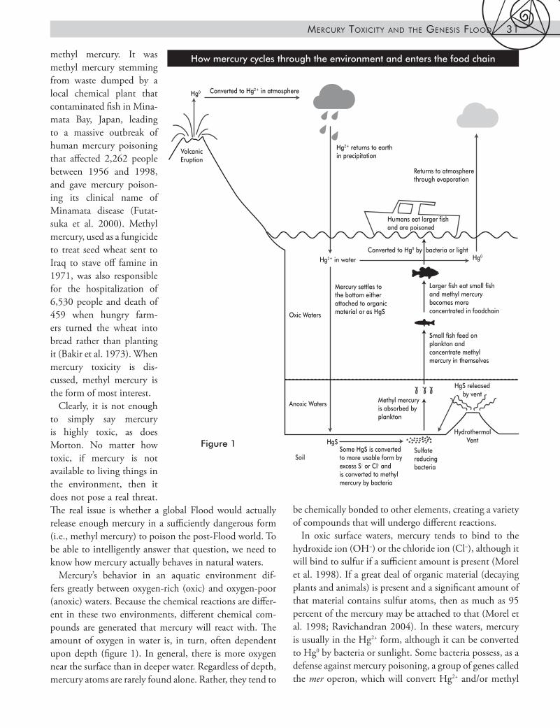
header about below be sure to check caption for repeatHow mercury cycles through the environment and enters the food chain

Mercury ToxiciTy And The GeneSiS Flood 31

methyl mercury. It was methyl mercury stemming from waste dumped by a local chemical plant that contaminated fish in Mina-mata Bay, Japan, leading to a massive outbreak of human mercury poisoning that affected 2,262 people between 1956 and 1998, and gave mercury poison-ing its clinical name of Minamata disease (Futat-suka et al. 2000). Methyl mercury, used as a fungicide to treat seed wheat sent to Iraq to stave off famine in 1971, was also responsible for the hospitalization of 6,530 people and death of 459 when hungry farm-ers turned the wheat into bread rather than planting it (Bakir et al. 1973). When mercury toxicity is dis-cussed, methyl mercury is the form of most interest.

Clearly, it is not enough to simply say mercury is highly toxic, as does Morton. No matter how toxic, if mercury is not available to living things in the environment, then it does not pose a real threat. The real issue is whether a global Flood would actually release enough mercury in a sufficiently dangerous form (i.e., methyl mercury) to poison the post-Flood world. To be able to intelligently answer that question, we need to know how mercury actually behaves in natural waters.

Mercury’s behavior in an aquatic environment dif-fers greatly between oxygen-rich (oxic) and oxygen-poor (anoxic) waters. Because the chemical reactions are differ-ent in these two environments, different chemical com-pounds are generated that mercury will react with. The amount of oxygen in water is, in turn, often dependent upon depth (figure 1). In general, there is more oxygen near the surface than in deeper water. Regardless of depth, mercury atoms are rarely found alone. Rather, they tend to

be chemically bonded to other elements, creating a variety of compounds that will undergo different reactions.

In oxic surface waters, mercury tends to bind to the hydroxide ion (OH−) or the chloride ion (Cl−), although it will bind to sulfur if a sufficient amount is present (Morel et al. 1998). If a great deal of organic material (decaying plants and animals) is present and a significant amount of that material contains sulfur atoms, then as much as 95 percent of the mercury may be attached to that (Morel et al. 1998; Ravichandran 2004). In these waters, mercury is usually in the Hg2+ form, although it can be converted to Hg0 by bacteria or sunlight. Some bacteria possess, as a defense against mercury poisoning, a group of genes called the mer operon, which will convert Hg2+ and/or methyl

Figure 1


mercury to Hg0 (Kiyono et al. 2003; Wagner-Dobler et al. 2000). Thus, these bacteria convert the mercury from a more toxic form to a less toxic form, a fact that could have a significant impact on mercury’s behavior during the Flood. It is also possible for Hg2+ to be converted to Hg0 by light. In general, the reaction with light is most impor-tant if the mercury concentration is too low to activate the mer operon; otherwise, the bacterial route dominates (Morel et al. 1998). Once it has become Hg0, the mercury will evaporate into the atmosphere, be converted back to Hg2+ there, and return to earth elsewhere in rain. It is also possible for Hg2+ to be converted to methyl mercury in oxic water, but only if the concentration of Cl− is in the right range and the correct bacteria are present (Najera et al. 2005). Oxic surface waters are not considered a major area for methyl mercury production.

Higher concentrations of mercury are often found in anoxic waters (Mason et al. 1999; Morel et al. 1998). These include deeper waters and swamps or peat bogs, where bacterial decomposition of dead plant material uses up a great deal of oxygen and poor circulation fails to replenish it. The excess organic material helps make swamps natural mercury traps (United States Geological Survey [USGS] 2004), since this organic material will bind the mercury and the sulfate-reducing bacteria common in these envi-ronments will convert sulfate to sulfide, the form of sulfur most reactive with mercury. The sediments below deeper anoxic waters also contain these bacteria, accounting for their higher concentrations of sulfide (and therefore mer-cury) than the oxic waters above. In fact, mercury chem-istry in anoxic environments is dominated by its reaction with sulfide (Morel et al., 1998). The primary compound formed by the reaction of mercury with sulfide is mer-cury sulfide or cinnabar (HgS). Most of the mercury in sediments is, in fact, found as cinnabar (Greenwood and Earnshaw 1984). Cinnabar itself is highly insoluble, so formation of cinnabar would have the net effect of remov-ing mercury from water. Cinnabar can form more soluble compounds in the presence of other sulfides (Morel et al. 1998), elemental sulfur (Morel et al. 1998), acidic waters containing Cl− (Mikac et al. 2003), or excess organic material (Ravichandran 2004).

Not only are sulfate-reducing bacteria partly to blame for increased mercury concentrations in anoxic waters, they are also the source of deadly methyl mercury (Morel et al. 1998). An enzyme in these bacteria will convert Hg2+ to methyl mercury (Choi et al. 1994). The methyl mercury is then absorbed by one-celled organisms, which are in turn eaten by larger organisms. In this way, the

mercury moves up the food chain. For example, if 10 percent of the total mercury in an aquatic ecosystem is methyl mercury, approximately 15 percent of the mer-cury in tiny phytoplankton would normally be methyl mercury, increasing to 30 percent in the zooplankton that feed on the phytoplankton, and 95 percent in the fish near the top of the food chain (Morel et al. 1998) (figure 1). This can result in significant amounts of methyl mer-cury accumulating in the top predators, which can be toxic if eaten by humans.

Therefore, Morton greatly oversimplifies the problem. Fish have a very low uptake rate for Hg2+ and will not accumulate significant amounts of it (Morel et al. 1998). High levels of Hg2+ are of concern primarily because of its ability to be converted to methyl mercury. In fact, the U.S. Environmental Protection Agency (EPA) is consid-ering setting new groundwater mercury standards based not on the total concentration of mercury in the water, but on the concentration of methyl mercury in fish living in a body of water (Southworth et al. 2004). Even in the Everglades, an almost ideal environment for methyl mer-cury production, only 20 percent of the total mercury is methyl mercury (Cai et al. 1999). By comparison, only 3 percent of the total mercury dissolved in rivers and 2 per-cent in coastal ocean waters is methyl mercury (Mason et al. 1999). One more recent study found that between 1.2 and 17.2 percent of the total mercury in peaty stream banks was methyl mercury, while less than 1 percent was methyl mercury in the soil 65 feet (20 m) from the stream (Skyllberg et al. 2003), while another found that 0.3 percent and 8 percent of the total mercury in a number of Virginia and Tennessee streams was methyl mercury (Southworth et al. 2004). Therefore, of the mer-cury released by the Flood, less than 20 percent (probably closer to 1 percent) would have been methyl mercury. Furthermore, we must keep in mind that methyl mer-cury poisoning is not an instantaneous process. We learn from the great mercury poisoning incident in Minamata Bay, Japan, that mercury began to be dumped into the bay in the 1930s, yet symptoms of poisoning were not reported in humans until approximately 20 years later, and at least a year after new procedures at the plant sig-nificantly increased the amount of mercury released (Eto 2000; McCurry 2006).

Historically, mercury has had a number of industrial uses and has therefore been mined as a mineral. Approxi-mately three-quarters of the world’s mercury production comes from just five major mercury belts (Rytuba 2003). Since these represent a major reservoir of mercury in


today’s environment, they are of great importance for our discussion of mercury and the Flood.

Geologic mercury is usually found in one of three types of deposits: Almaden-type deposits, silica-carbonate deposits, and hot spring deposits (Rytuba 2002). More than one-third of all mercury mined worldwide comes from the world’s largest cinnabar deposit near Almaden, Spain (Jebrak et al. 2002), the type of locale for Almaden-type deposits. These ores formed from large submarine hydrothermal vents or submarine volcanoes. Although there is still some debate as to exactly how and when the Almaden deposit was created, the consensus seems to be that the main deposits were deposited from hydrother-mal fluids as, or shortly after, the sedimentary rock layers containing them formed, while secondary deposits were formed by the remobilization of that mercury, perhaps in conjunction with the introduction of new hydrothermal mercury during later hydrothermal events (Hernandez et al. 1999; Hugueras et al. 1999; Jebrak et al. 2002). The layer of rock (primarily the rock quartzite) containing the mercury has been assigned to the Silurian age (Hernandez et al. 1999; Rytuba 1986a). This is a geological period that young-Earth geologists believe corresponds to a time early in the Flood (Whitmore 2007), consistent with the Almaden volcanic/hydrothermal activity being part of the erupting “fountains of the deep.”

Silica-carbonate mercury deposits are found along fault zones associated with the mineral serpentinite (Rytuba 2002, 2003), which has been transformed by an influx of carbonate and silica from low-temperature hydrothermal fluids (Rytuba 2002; Sherlock and Logan 1995). These fluids also contained mercury, which was deposited as cin-nabar along fractures in the altered serpentinite (Rytuba 1986b; Sherlock and Logan 1995). These are believed to have formed during the Tertiary, well after the Almaden deposit (Ash 1996; Rytuba 1986b), and are often asso-ciated with “prehistoric” mineral springs (Sherlock and Logan 1995).

Hot spring mercury deposits form in similar fashion, but with hotter hydrothermal fluids (Sherlock and Logan 1995). They are not associated with serpentinite (Pan-teleyev 1996; Rytuba 2002) and often occur in environ-ments nearer to the surface than silica-carbonate deposits (Rytuba 2002). Some are still forming today in places like Sulphur Bank, California (Sherlock and Logan 1995). Although not usually classified as one of the three major deposit types, the world’s second largest mercury deposit occurs at Idrija, Slovenia. It is believed to have formed in a manner similar to hot springs and silica-carbonate

deposits with hydrothermal fluids infiltrating through already-established sedimentary rock layers and deposit-ing mercury. However, a significant amount of mercury also may have been in the black shale present prior to hydrothermal enrichment (Lavric and Spangenberg 2003). The association between mercury and black shale will be discussed later.

With this brief overview in mind, let’s examine the first key question relating to Morton’s challenge: would the Flood release sufficient mercury to create an average con-centration of 100 ppb worldwide?

How Much Mercury Would the Flood Release?

Morton assumes that there was little to no sedimentary rock present before the Flood and that the current volume of sedimentary rock corresponds to the amount of igne-ous rock crushed and redeposited by the Flood. While this is probably an overstatement, we can use it as a maximum for Flood erosion. Morton then assumes that Earth’s crust contains 0.1 ppm mercury and that erosion would release 90 percent of that mercury, leading to a 100 ppb aver-age mercury concentration in the world’s waters. Morton considers 0.1 ppm a “very conservative” estimate, basing this number on a USGS report (Parker 1967). This report actually listed three values for mercury in Earth’s crust and two for igneous rock. In both cases, the oldest value was 0.5 ppm, while newer estimates were approximately 0.08 ppm. More recent papers estimate 0.05 ppm (Lavergren 2005; United Nations Environment Progamme 2003).

Therefore, 0.1 ppm is not conservative; if anything, it seems a little high. Furthermore, these estimates are for the mercury concentration of the modern crust. If the major mercury deposits observed today (such as Almaden) were formed during or after the Flood, pre-Flood crustal mercury might have been much lower, especially since it appears that they formed by mercury migrating in hydrothermal fluids from Earth’s interior. Perhaps a better estimate would come from looking at the mercury concentration in the bulk silicate earth, which includes the crust and mantle. This might better approximate the primitive mantle prior to the formation of a true crust (Baumgardner 2000; Kargel and Lewis 1993; McDonough and Sun 1995). This number would be 10 ppb, or 0.01 ppm, an order of magnitude less than Morton’s “conservative” estimate (Baumgardner 2000; McDonough and Sun 1995). However, that is only his first error.

Morton’s 90 percent estimate of mercury mobilization comes from a USGS paper (Siegel and Siegel 1987)


discussing mercury being released by volcanoes in Hawaii. Volcanoes are a major source of mercury; significant spikes in total atmospheric mercury correspond to volcanic eruptions (Schuster et al. 2002). Morton refers to a section of this paper that discusses mercury lost by erosion of a cooled lava flow. However, the context is the slow release of mercury from the lava flow over a century. Morton apparently assumes that the same amount would be released by rapid weathering (over the course of perhaps days) during the Flood. However, this assumption appears flawed. To understand why, let’s take a closer look at the paper Morton is referencing, one paragraph of which is quoted by Morton. Here is the paragraph directly preceding the one he quotes:

Lava flows constitute another source of mercury. Weathering brings about the slow release of soluble or solubilized constituents as the igneous materials degrade into soil minerals. Lava samples were analyzed by digestion of 100-mesh powder with 0.1 N HCl to remove soluble and loosely bound mercury. This was followed by hot 2N HN03 digestion to remove any mercury complex with organic ligands, and then concentrated HF to destroy the silicate matrix (Siegel and others, 1975). Samples from flows of 1840, 1923, and 1955 were obtained with the assistance of the late Gordon Macdonald; fresh Pauahi samples were collected in 1979. The results . . . suggest a 50 percent release in about 50 years and a gradual infiltration of oxidizable, presumably humic, complexing substrates (Siegel and Siegel 1987, p. 832–833).

This paragraph is followed by a table (see table 1) listing how much mercury was removed from rock samples of different ages by each of the three methods described above. The estimate of 90 percent mercury loss over the course of 100 years comes from comparing the total amounts of mercury (from all three measurement

methods) for samples of different age. However, this is not the only significant thing we can learn from this data. For all the samples, the 0.1N HCl (HCl is a strong acid and normality [N] is a unit of concentration, a 0.1N solution of HCl would have a pH of 1) removed only a small amount of the total mercury. For every sample but the oldest, the 2N HNO3 removed far less mercury than the concentrated HF.

Morton states that sedimentary rocks in the Flood were formed from mechanically crushed and chemically weathered igneous rocks, releasing mercury in the pro-cess. The igneous rocks in the study he cites were crushed, then treated with various acids to remove the mercury for analysis. This laboratory procedure was probably more chemically destructive and therefore more likely to release mercury than anything occurring during the Flood. Fur-thermore, it is clear that only the most extreme labora-tory conditions actually removed the majority of mercury from these samples. Digestion in 0.1N HCl is a very chemically destructive process, and 2N HNO3 is slightly more than an order of magnitude more acidic (plus more chemically reactive in other ways) than 0.1N HCl. Yet only in the sample from 1840 was more than 21 percent of the total measured mercury removed by the HCl and HNO3 combined. In that sample, roughly 66 percent of the total mercury was removed by both procedures. The HF was successful at removing the mercury not because it is a stronger acid than the others (it’s actually weaker), but because a specific chemical reaction between the HF and silicon in the igneous rock literally breaks up the chemical structure of the rocks (this is what the authors meant by “destroy the silicate matrix”). The authors concluded that the mercury released by HCl was only loosely attached to the rock. Mercury released by HNO3, on the other hand, was interpreted as being attached to organic compounds that had gradually entered the lava flow; HNO3 will destroy organic material through an oxidation reaction. However, organic material presumably was not destroyed by the Flood water, nor would the Flood water have resembled

Year lava flow formed

Hg extracted by HCl (ppb)

% of total Hg extracted by HCl

Hg extracted by HNO3 (ppb)

% of total Hg extracted by HNO3

Hg extracted by HF (ppb)

% of total Hg extracted by HF

1840 5 3.82% 81 61.8% 45 34.4% 1923 16 4.08% 66 16.8% 310 79.1% 1955 10 0.962% 59 5.68% 970 93.4% 1979 0 0.00% 15 1.15% 1,290 98.8%

Table 1. The extraction of mercury from cooled lava flows (Siegel and Siegel 1987)


concentrated HF. Therefore, the digestion in HCl is prob-ably the only process analogous to those of the Flood, and the Flood water would have been less acidic than the HCl. For the two oldest lava samples, approximately 4 percent of the mercury was removed by the HCl; in other words, only 4 percent of the mercury was readily soluble in very acidic water even after the rocks were physically pulver-ized, and not the 90 percent suggested by Morton!

This would not be surprising to any chemist; most of the mercury would be in the form of mercury sulfide, which is extremely insoluble. Mercury does not become a pol-lution problem because large amounts of mercury sulfide will dissolve in water; rather, the mercury either enters the water in a more soluble form or very tiny amounts of mercury sulfide dissolve and are then (over time) magni-fied up the food chain. Many studies have documented the insolubility of HgS, even in strong acids (Fernandez-Martinez and Rucandio 2003, 2005; Martin-Doimeadios et al. 2000; Mikac et al. 2003). Excess Cl− is required to make mercury sulfide soluble. How much Cl− would have been available during the Flood? At present, it is estimated that the crust only contains 185 ppm chlorine (Parker 1967), while that in the silicate earth is estimated at 17 ppm (McDonough and Sun 1995). Even the higher figure (assuming all of it converted to soluble Cl− and using the same figures Morton used to estimate the concentration of mercury in Flood water) only corresponds to 0.00586 N Cl−. This is approximately 17 times less Cl− than is present in 0.1N HCl, which was ineffective in extracting mercury. Mikac et al. (2003) noted that in the presence of 0.01N Cl−, greater than 1N HNO3 was required to extract significant amounts of mercury. The Flood water simply would not have been that acidic.

Although this fact is not mentioned by Morton, it has also been reported in the literature (Revis et al. 1989; Han et al. 2008) that a saturated solution of sodium sulfide will extract significant amounts of mercury from HgS-contaminated soils. The reality is that moderate or low concentrations of sulfide will remove mercury from water as HgS and prevent its redissolving (Piao and Bishop, 2006), while high concentrations will render it soluble again. However, using calculations such as those used for chlorine in the preceding paragraph, it is clear that even if all the sulfur in the earth’s crust was dissolved and converted to sulfide, the resulting Flood waters would contain a much lower concentration of sulfur than a satu-rated Na2S solution would; sodium sulfide is very soluble! Therefore, this would not significantly help Morton to get the HgS in the earth’s crust dissolved. In fact, the sul-

fide in the Flood waters would most likely have been at a low enough level (once the interaction of sulfur with other elements in the water is considered) to significantly decrease the solubility of the mercury. Han et al. (2008) also showed that mercury can be somewhat more easily extracted from HgS residing in soil that has been planted with crops for several seasons. However, only a small frac-tion of the crust destroyed by the Flood would have been topsoil involved in agriculture and much stronger acids than we would expect in the Flood waters were required to extract the mercury in that study. These findings do not make Morton’s thesis any more believable.

For the last word on this subject, Professor Donard, an environmental chemist from France who studied the extractability of mercury sulfide from the mines at Almaden, Spain, noted (Martin-Doimeadios et al. 2000, p. 365):

The total extraction results and the sequential extraction procedure have shown that mercury in the Almaden’s sediments is quite stable and presents low chemical availability. This lack of availability renders inorganic mercury methylation difficult. The results are consistent with mineralogy of mercury deposits, since cinnabar has an extremely low solubility in water, is resistant to physical and chemical weathering, and is hardly leached under acid drainage.

Although Morton’s basic thesis is clearly in error, let’s examine other ways that mercury could get into the Flood environment. First, the 40 days and nights of rain would have moved essentially all of the mercury from the atmosphere. However, this would have been insig-nificant: even after more than a century of industrial activity, which has dramatically increased the amount of mercury in the atmosphere (Schuster et al. 2002), there are only 6,000–10,000 tons of mercury there today (Lin and Pehkonen 1999). In the pre-Flood world, atmo-spheric mercury would have presumably been much less. Second, volcanoes would have released mercury, and we assume a tremendous amount of volcanic activity during the Flood. Likewise, undersea hydrothermal vents would have released mercury (Ruelas-Inzunza et al. 2003). If the “fountains of the deep” mentioned in Genesis 7:11 indicate hydrothermal activity, these might have been a significant source of mercury pollution (although for reasons I will explain later, I somewhat doubt it). Over-all, these processes probably elevated the amount of mercury in the Flood environment. Still, given Morton’s


miscalculation of both the total available mercury and the percentage released into the environment, the total concentration would have been considerably less than Morton’s 100 ppb.

So what is a more reasonable estimate for the amount of mercury released by the Flood? From the outset, I want to acknowledge that this is not a simple ques-tion; as has already been shown, there would have been a number of factors affecting mercury concentration (many of which simply cannot be determined millennia later), and therefore the best that can be provided is a rough estimate. However, I believe I can at least give an estimate that is closer to reality than Morton’s. To start with, in place of Morton’s too high estimate of 0.1 ppm, let’s use Lavergren’s 0.05 ppm value (Lavergren 2005; United Nations Environment Programme 2003), which immediately cuts Morton’s number in half and equates to 50 ppb mercury in the Flood waters. Also, since Mor-ton’s assumption that 90 percent of the mercury in the crust would be dissolved is far too high, let’s reduce that to a more reasonable value of 5 percent. (In light of the extreme insolubility of mercury sulfide, I think this is a generous estimate.) That would reduce the concentration to 2.78 ppb in the Flood waters. If we started with the bulk silicate earth mercury value of 0.01 ppm for the crust’s concentration (Baumgardner 2000; McDonough and Sun 1995), that would reduce the final value by a factor of five, giving a final concentration of 0.56 ppb mercury. Admittedly, my assumption that 5 percent of the mercury would dissolve, while in line with the pub-lished data, might be downplaying the unique properties of the Flood. If we assume that my estimate of mercury solubility is too low and arbitrarily triple it to 15 percent, that still results in mercury concentrations of less than 10 ppb, a tenth of Morton’s estimate. So I would conclude that there was between 0.5 and 10 ppb mercury in the Flood waters, with the real value probably lying closer to the smaller number. Furthermore, no more than 20 percent, and probably closer to 2 percent, of this would be the deadly methyl mercury. As we will see in the next section, while such a concentration is far from desirable, it is not catastrophic.

So Morton’s estimate of mercury released by the Flood is massively too high. However, for the sake of argument, let us assume that Morton is right and the Flood water con-tained 100 ppb mercury for our evaluation of the second big question: the threat such a release would actually pose to the environment.

Was Mercury a Threat to the Post-Flood World?

It is not enough for sufficient mercury to be released to yield a 100-ppb concentration in the Flood water. The mercury must have remained dissolved for enough time to have worked its way into the food chain. As noted above, the Flood water would represent a very complex chemi-cal system. A mercury concentration near 100 ppb would have presumably activated the bacterial mer operon, so bacteria would have been converting Hg2+ to Hg0, which would evaporate into the atmosphere. Morton argues in his paper that Hg0 evaporation would not be an issue because the continual rainfall during the Flood would have removed it from the atmosphere. Although that would be true for the 40 days and 40 nights of rainfall, it was during this period that the Flood water was still rising, and pre-sumably the mercury had not then reached its maximum concentration. Once the rain ended, mercury could begin to accumulate in the atmosphere, lowering the concentra-tion in the water. However, the interplay between evapo-ration and precipitation would probably prevent this from being a major form of mercury removal.

There would have been a great deal of organic matter (decomposing plant and animal life) in the Flood water. This organic matter would have trapped a major amount (current studies suggest as much as 95 percent) of the mercury. If this organic bound mercury was in an oxic environment, it is unlikely that it would have been con-verted to methyl mercury. Thus it would pose a smaller threat because aquatic animals would not have retained Hg2+ to the same degree as methyl mercury. Morton does not make this distinction, simply noting that the U.S. EPA’s permissible concentration for mercury in drinking water is 2 ppb and assuming anything above this concen-tration would be problematic. Obviously, any significant concentration of mercury in drinking water is not good; however, it is naïve to simply assume that the EPA limit represents the absolute maximum mercury concentration above which great harm occurs. The truth is that many humans routinely drink a liquid with greater that 2 ppb mercury, namely our saliva. The amalgams used for dental fillings contain a significant concentration of mercury, and that mercury tends to find its way into saliva. One study found that people with amalgam fillings have saliva mercury concentrations anywhere from 0 ppb to 500 ppb, with an average of ~3.5 ppb before chewing and ~31.5 ppb after chewing (Ganss et al. 2000). These values were reported to be in good accord with previously published


values. A slightly more recent study of Hg2+ leaching from amalgams into simulated saliva reported a concentration of 15 ppb after 6 hours of contact with the amalgam and 101 ppb after 90 hours contact (Sanna et al. 2002). While it is outside the scope of this paper to discuss the contro-versy over the health effects of mercury dental amalgams, it is worth noting that human life is not being imperiled by ingesting concentrations of Hg2+ greater than the EPA drinking water limit and approaching Morton’s too-high estimate for the Flood water. The primary health threat from mercury does not come from ingesting water con-taining Hg2+.

In an anoxic environment, on the other hand, a sig-nificant amount of methyl mercury could begin to form. This would have been the real threat: the formation and availability of sufficient methyl mercury to infiltrate the food chain and poison life. However, only a relatively small amount of the total mercury in a system is nor-mally methyl mercury. Under ideal anoxic conditions, it would reach no more than 20 percent of the total; in less ideal conditions, it would have been only 2–3 percent of the total. So, even if the total concentration of mercury reached 100 ppb, we would only expect ~2–20 ppb to exist in that dangerous form. In reality, it was probably less than that.

In a previous section, I mentioned that hydrothermal vents could have been a source of mercury contamination for the Flood. However, it is also possible they removed mercury from the system. Not only do these vents release mercury, they also release hydrogen sulfide, and sulfides react with mercury to form insoluble mercury sulfide. Therefore, excess sulfide would have removed mercury the vent released, forming cinnabar deposits. Mercury in the Flood water near the vent would also have been captured.

The Almaden mercury belt described earlier could be an example of this process. The source of mercury at Almaden was hydrothermal fluids and magma released during elevated hydrothermal activity, probably during the Flood. The mercury is believed to have been deposited at the same time that the surrounding sedimentary rock was forming or after it had formed. Since sedimentary rocks would have formed rapidly during the Flood, and since the vents were at the interface of the Flood water and the seafloor (including former continental surfaces), the vents and associated mercury were buried by Flood sediment. This is not only consistent with the geology of the Almaden deposit, but would have resulted in limiting the deposit’s contribution to contamination of the Flood water. Modern hydrothermal systems tend to be sources

of mercury pollution, but during the Flood they were more likely sinks, chemically binding free mercury that was then rapidly covered by thick sediments.

Since deepwater vents would also coincide with anoxic environments, this entrapment of mercury would pref-erentially lock up the more dangerous methyl mercury, in my opinion. Mercury methylation in the Flood would have been occurring in deeper waters, where organic mate-rial would have been sinking down and decaying, helping to deplete the water of oxygen. With most of the mercury being bound to organic material or occurring as mercury sulfide, it would have been settling to the bottom anoxic zone as well. Normally this would generate excess mercury methylation, but in the Flood, it would have only trapped mercury in the new sedimentary rocks.

There is still debate as to the average concentration of mercury in sedimentary rock (Parker 1967; Yudovich and Ketris 2005). However, black shales are enriched with mercury, with concentrations perhaps as much as an order of magnitude above the average of other sedi-mentary rock (Lavergren 2005; Parker 1967; Yudovich and Ketris 2005). Also, there is still a significant debate in the geological literature as to how black shales form (Kenig et al. 2004; Lavergren 2005; Lyons and Kashgar-ian 2005; Schultz 2004). The consensus seems to be that they represent at least intermittently anoxic environments rich in organic material and sulfides. Such an environ-ment would trap mercury, both in its organic material and by hydrogen sulfide generated by the sulfate-reduc-ing bacteria expected to flourish there during anoxic peri-ods, and promote its methylation. We know these sedi-ments were converted into rock. And we know that these rocks contain a great deal of mercury, probably averaging between 0.4 and 0.22 ppm (Lavergren 2005; Parker 1967; Yudovich and Ketris 2005). While all the black shale seen today likely did not form during the Flood (some of it appears rather late in the geologic column for that), it is reasonable to assume that much of it did. The mercury in these shales represents a tremendous quantity that was effectively removed from the system by sedimentation. Furthermore, since the environment that most likely formed the black shales would have been conducive to mercury methylation, this would have removed the mer-cury most likely to be transformed into methyl mercury. Similarly, coal is often enriched in mercury (Yudovich and Ketris 2005). Rapid coal formation during the Flood would likewise bind great amounts of mercury from the environment. Please recall that the process of converting Hg2+ to methyl mercury and then infiltrating it into the

HgS HgS

HgS HgS HgSHgS HgS

HgSHgS

HgS

HgS

HgS

Hydrothermalvents releaseH2S, which reactswith mercury to form mercury sulfide

Organicmaterial trapsmercury, then settlesto the bottom

Mostmercuryin form ofinsolublemercurysulfide, whichsettles tobottom

Flood waters contain a tremendous amount of sediment,including mercury

Further sediment settles from the Flood waters, burying the previously precipitated mercury

HgS HgSHg2+ Hg2+

Hg2+ Hg2+ Hg2+

Hg2+

Hg2+

Hg2+

Hg2+

Hg2+

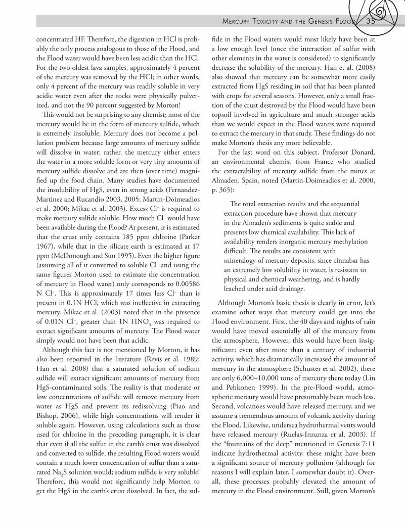
Mercury header about chart below be sure to check caption for repeatProcesses removing mercury from the Flood waters


food chain in hazardous quantities is not fast. The rapid sedimentation of the Flood would have prevented this from occurring to any great extent.

A recent study (Orihel et al. 2008) supports this view. The authors added mercury spiked with various radioac-tive elements (so they could track the specific mercury they had added) to an experimental lake once a year for two years. They found that most of the mercury they added the first year had found its way into the sediment by the second year. A similar study (Tessier et al. 2007) using aquariums as simulated bodies of water found that most (87.9–96.2 percent) of the mercury added had found its way into the sediment within a month. Orihel and coworkers also found that most of the mercury was not converted to methyl mercury, and much of the methyl mercury that was produced remained in the sedi-ment and was not available to be consumed by many of the organisms. This was occurring in an environment with much slower sedimentation than the flooded earth. The best evidence suggests that natural processes would have buried much of the mercury released by the Flood before it entered the foodchain (figure 2).

Even in areas where mercury methylation could occur without being removed by sedimentation, there is reason

to believe that net methylation of mercury would have been less than predicted. This is because the Flood would have been an “equal opportunity” polluter; the waters would have contained more than just mercury. Using Morton’s methods, we see that the same rocks contain approximately 5 percent iron (Parker 1967). The silicate earth concentration is estimated at between 18 and 19 percent (McDonough and Sun 1995). In either case, there would have been a great deal of iron in the Flood water. Studies have shown that high concentrations of iron will decrease the rate of mercury methylation (Mehrotra and Sedlak 2005). In fact, those authors suggest adding iron to wetland sediments as a way to decrease methyl mercury pollution. Between the rapid sedimentation and the high concentration of iron in the Flood water, it seems unlikely that methyl mercury formation posed a great problem during the Flood.

Morton suggests that the high concentration of Hg2+ in the Flood water would have harmed plant life, even if it was not methyl mercury. Of course, we have already established that total mercury in the Flood water was much less than Morton’s 100 ppb, but for the sake of argument, let’s grant him that figure. To support his contention that this would have been devastating to

Figure 2


plant life, Morton references some data suggesting that “typically, plant-cell damage takes place with aqueous solutions containing as little as 10 [micro]g/L of Hg ion” (Morton 1998). This comes from the same paper (Siegel and Siegel 1987) on mercury and volcanoes that Morton used to get his estimate of 90 percent mercury loss during weathering. We have already seen that his presentation of that data required further scrutiny. Thus, it comes as no surprise that this one does, too.

Siegel and Siegel (1987) only mentioned this figure in passing to set up a contrast with the relatively low toxic-ity of Hg0 to plant life. They cite a paper (Siegel 1977) as the original source of the data. If we look at this original paper, we see that Morton’s figure for plant damage, while presumably made in good faith, is misleading. That is because the ten micrograms per liter value in the original paper was not referring to “plants growing in mercury-rich ground water [sic]” as Morton states, but to tobacco protoplasts. A protoplast is a cell without its protective cell wall. In this case, the author wanted to see how toxic some metals were to plant cells if they got through all the plant’s defenses and actually reached the cell. Although this is an important topic for study, it is not a very realis-tic analogy of how the whole organism would respond to mercury, nor was it intended by the author to be taken in that way. Still, even accepting that this study is showing the tobacco cells at their most vulnerable state, it should be noted that, while cell damage may have occurred at a 10 ppb concentration, 100.3 ppb was required to kill 50 percent of the protoplasts. In the Flood, plants did not exist as lone protoplasts, but rather as seeds or shoots that later grew into mature organisms. Therefore, a far more realistic appraisal of mercury toxicity to plants would be the concentration required to inhibit seed germination. The seed, of course, contains multiple cells with cell walls and, therefore, as Siegel stressed in this paper, is more resistant to poisoning. In fact, he reported that a concen-tration of approximately 802 ppb was required to inhibit the germination of 10 percent of the tobacco seeds, and that slightly over 2,200 ppb were necessary to prevent 50 percent from germinating.

This is not an isolated example. To the contrary, as Morton should have realized, the ability of plants to survive in waters containing very high mercury concentrations has been reported many times in the literature. For example, a more recent paper concerning mercury toxicity to tobacco states, “Tobacco has been shown to be highly resistant to environmental mercury, accumulating up to 5,000 μg/g under chronic low-level exposure with no symptoms of

toxicity” (Suszcynsky and Shann 1995). This means the tobacco can accumulate within it 5,000 ppm mercury without seeing any ill effect. Now, one might argue that this is only referring to chronic low-level exposure, not a sudden high-level exposure such as the Flood could cause. The paper addresses this as well. The author submerged the roots of tobacco plants in solutions with varying concen-trations of mercury and observed the effects on the plants. Keep in mind that Morton’s estimate for mercury in the Flood water (far too high to begin with) is only 100 ppb or 0.1 μg/ml. Suszcynsky and Shann (1995, p. 65) noted:

An inhibition of whole plant growth was demonstrated in plants whose roots were exposed to HgCl2 with the severity of inhibition corresponding to increasing treatment levels. Plants at higher treatment levels (>10.0 μg Hg2+/ ml) displayed minor visible symptoms of toxicity (chlorosis) but no tissue death. . . . Although growth in plants exposed to lower treatment levels (≤ 1.0 μg Hg2+/ ml) was slightly inhibited, there was no apparent threat to their viabilityas that which occurred in plants exposed to higher treatment levels.

In other words, the survival of the tobacco plants was not threatened by a mercury concentration ten times higher than Morton’s estimate, and there was no actual tissue death in plants to a concentration ten times higher than that! Tobacco is not the only plant resistant to mer-cury. Another study reported that 47 percent of alfalfa seedlings exposed to an approximately 600 ppb Hg2+ solution for 24 hours showed no ill effect, and 11 percent showed no effect after 24 hours’ exposure to 6,000 ppb mercury (Ortega-Villasante et al. 2005). Seedlings from two types of rice were shown to undergo slightly over 50 percent germination in a solution of more than 20,000 ppb mercury, while the germination rate was between 70 and 80 percent in a solution a tenth as concentrated (Mishra and Choudhuri 1999). While these may have been far from healthy rice plants, they were surviving in waters that contained orders of magnitude more mercury than even Morton suggests the Flood would have con-tained. A study of the aquatic plant Vallisneria Spiralis did not note ill effects on plants from exposure to any concentration less than approximately 200 ppb mercury (Gupta and Chandra 1998). Water lettuce is reported as surviving, albeit with complete inhibition of new root formation, for three weeks (the plants did not all die at the end of three weeks, the study just ended) in solutions of


over 100,000 ppb mercury (Odjegba and Fasidi 2004). In fact, the author of that study suggested that these plants could be used to remove mercury from polluted waters, a process known as phytoremediation. The water hyacinth has also been suggested for phytoremediation due to its ability to survive in mercury-contaminated waters and accumulate the mercury within itself (Riddle et al. 2002). To summarize all of this, many plants can survive expo-sure to concentrations of mercury many times higher than Morton claimed would be lethally toxic during the Flood. Clearly, his estimates of mercury toxicity are just as con-fused as his calculations of mercury concentration in the Flood water.

Conclusions

Based upon an honest look at the available evidence, Morton’s challenge to the Genesis Flood does not stand. First, earth’s crust at the time of Noah likely did not con-tain the 0.1 ppm mercury he estimated. Even if it had, it is unlikely that the Flood would have released more than a small percent of that mercury, much less 90 percent. And even if that much mercury were released, it would have been removed from the water by: (1) binding to organic matter, (2) precipitation as a sulfide, and (3) rapid burial by sedimentation (figure 2). Furthermore, to enter the food chain, the mercury would need to be converted to methyl mercury, and both sedimentation and the iron released by the Flood would have inhibited that. Finally, even if the concentration of mercury did reach 100 ppb, plant life still would have survived. There is no reason to question the Genesis account based on mercury chemistry.

While this paper has been focused on that one specific contaminant, I am confident that careful study will show that the release of other environmental toxins also fails to threaten the Flood model.

Appendix 1: Morton in His Own Words

It [Morton’s paper] will consider the amount of mercury (element symbol Hg) that must have been released by the erosion of the pre-Flood igneous type of rock which was then made into sedimentary rock containing fossils. The YEC [Young Earth Creationist] paradigm requires that there be very little sedimentary rock prior to the flood. This is because none would have been made at creation (it would be a deception to make rocks appear sedimentary which were in fact not sedimentary). Thus we can calculate how much igneous rock must have been eroded to form the presently observed volcanic rocks. The total of sedi-mentary rocks can be calculated as 630 x 10^6 km^3. (See

R. Morton [this is me] “Prolegomena to the Study of the Sediments,” CRSQ, Dec. 1980, p. 162–167). All of this material must have come from igneous rock.

Given that igneous rocks are around 3.3 g/cc (3300 kg/m^3) and sedimentary rocks are around 2.5 g/cc, we can correct for this and we find a .75 reduction factor to put the sedimentary rocks back to igneous. Thus, 477 x 10^6 km^3 or 4.77 x 10^17 cubic meters of igneous rocks must have been eroded.

An earlier version of this note was criticized for not making explicit an assumption. The assumption is this. Within the YEC model, the prediluvial rock, which mostly would have been granite and basalt, must have been mechanically crushed, and then rapidly altered chemically to separate the feldspar and quartz fractions. Only in this way can the vast quantities of sand and shale seen in the sedimentary rocks be explained. For God to have created the vast quantities of sand and shale on the primeval earth would be a case of God deceptively creating the appear-ance of age when no such appearance would be needed. On the primeval earth, only a thin layer of soil would be required, not 40 to 60,000 feet of it. By the process of mechanical crushing and rapid chemical weathering, much of the mercury contained in the rock would have been released. This is consistent with what is known to occur in the weathering of basalts in which 90 percent of the mercury in the basalts is released to the environment in about a century.

“If Kilauea lava typically cools with about 1,000 [micro]g/kg of mercury and proceeds to release 90 percent, then this still constitutes only a minor source of the element. The 1840 eruption produced about 400 x 10^6 m^3 of lava weighing perhaps 16 x 10^9 kg. Thus this lava con-tained a total of 16 x 10^6 g (16 tons) of mercury, of which about 14 tons was released in about a century. In contrast, Halemaumau yields 260 tons annually when it is not erupting” (Siegel and Siegel 1987, p. 833).

What is the mercury content of the crust of the earth? Using the very conservative value of .1 parts per million (ppm) we find that the flood would have ground up and released .0000001 * 4.77 x 10^17 cubic meters x 3300 kg/m^3 x .9= 1.4 x 10^14 kg or 1.4 x 10^17 g or 1.4 x 10^23 micrograms. I place this in all three units because of the need below.

All of this would have been released into the oceans for the fish to ingest. The volume of the ocean is 1.4 x 10^21 liters. So the amount of mercury in a liter is 1.41 x 10^23 micrograms/1.4 x 10^21 liters = 100 micrograms per liter of water.


How bad is it? Consider this: “Typically, plant-cell damage takes place with aqueous solutions containing as little as 10 [micro]g/L of Hg ion” ( Siegel and Siegel 1987, p. 830).

An expert might question the relevance of this fact to the Flood since the above refers to plants growing in mercury-rich ground water [sic]. Since plants were not taken on the ark, they must have survived by floating on the surface of the flood waters. And many young-earth creationists have suggested that such vegetable mats were responsible for the coal bed formation. Thus, the damage which mercury laden waters would cause to these floating plants is some-thing that must be addressed by global flood advocates.

The EPA does not allow more than 2.4 micrograms/liter, which is the EPA’s Critical Maximum Concentration for fresh water discharge from an industrial site. This was set up to protect aquatic life from deleterious effects from mercury (Gray and Sanzolone 1996, p. 5).

How about for animal ingestion? This was found on the Internet: “The EPA has set a limit of 2 parts of mercury per billion parts of drinking water (2 ppb = 2 micrograms/liter). The EPA requires that discharges or spills of 1 pound or more of mercury be reported” (http://atsdr1.atsdr.cdc.gov:8080/tfacts46.html).

For those who don’t know, 100 micrograms per liter is 50 times more than the EPA would allow for an anthro-pogenic release. I guess the EPA would initiate regulatory action against Noah’s Flood for polluting the oceans.

Acknowledgments

I would like to thank Dr. John Whitmore for eluci-dating many of the finer points of Flood geology to a simple chemist such as myself and for providing numer-ous editorial suggestions on this work. I would also like to thank Dr. John Reed for his significant editorial input. Finally, I would like to thank Dr. Heather Kuruvilla for useful guidance on the subject of protoplasts versus whole organisms.

ReferencesAposhian, H.V., R.M. Maiorino, D. Gonzalez-Ramirez, M. Zuniga-Charles, Z. Xu, K.M. Hurlbut, P. Junco-Munoz, R.C. Dart, and M.M. Aposhian. 1995. Mobilization of heavy metals by newer, therapeutically useful chelating agents. Toxicology 97:23–38.

Ash, C. 1996. Silica-carbonate mercury. In Selected British Columbia Mineral Deposit Profiles, Volume 2, Metallic Depos-its. British Columbia, Canada: British Columbia Ministry of Employment and Investment., p. 75–76.

Auger, N., O. Kofman, T. Kosatsky, and B. Armstron. 2005. Low-level methylmercury exposure as a risk factor for neuro-logic abnormalities in adults. Neurotoxicology 26:149–157.

Bakir, F., S.F. Damluji, L. Amin-Zaki, M. Murtadha, A. Kha-lidi, Y. Al-Rawi, S. Tikriti, H.I. Dhahir, T.W. Clarkson, J.C. Smith, and R.A. Doherty. 1973. Methylmercury poisoning in Iraq. Science 181:230–241.

Baumgardner, J.R. 2000. Distribution of radioactive isotopes in the earth. In Vardiman, L., A.A. Snelling, and E.F. Chaffin (editors), Radioisotopes and the Age of the Earth. El Cajon, CA: Institute for Creation Research, p. 49–94.

Bjorkman, L., G. Sandborgh-Englund, and J. Ekstrand. 1997. Mercury in saliva and feces after removal of amalgam fillings. Toxicology and Applied Pharmacology 144:156–162.

Boening, D.W. 2000. Ecological effects, transport, and fate of mercury: a general review. Chemosphere 40:1335–1351.

Brand, L. 1997. Faith, Reason, and Earth History: A Paradigm of Earth and Biological Origins by Intelligent Design. Berrien Springs, MI: Andrews University Press, p. 90–96.

Cai, Y., R. Jaffe, and R.D. Jones. 1999. Interactions between dissolved organic carbon and mercury species in surface waters of the Florida Everglades. Applied. Geochemistry. 14:395–407.

Choi, S.C., T. Chase Jr., and R. Bartha. 1994. Enzymatic catal-ysis of mercury methylation by Desulfovibrio desulfuricans LS. Applied and Environmental Microbiology 60:1342–1346.

Clarkson, T.W. 1998. Human toxicology of mercury. The Jour-nal of Trace Elements in Experimental Medicine 11:303–317.

Domingo, J.L. 1995. Prevention by chelating agents of metal-induced developmental toxicity. Reproductive Toxicology 9:105–113.

Eto, K. 2000. Minamata Disease. Neuropathology 20:S14–S19.

Fernandez-Martinez, R., and M.I. Rucandio. 2003. Study of extraction conditions for the quantitative determination of Hg bound to sulfide in soils from Almaden (Spain). Analytical and Bioanalytical Chemistry 375:1089–1096.

———. 2005. Study of the suitability of HNO3 and HCL as extracting agents of mercury species in soils from cinnabar mines. Analytical and Bioanalytical Chemistry 381:1499–1506.

Futatsuka, M., T. Kitano, M. Shono, Y. Fukuda, K. Ushijima, T. Inaoka, M. Nagano, J. Wakamiya, and K. Miyamoto. 2000. Health surveillance in the population living in a methyl mercury-polluted area over a long period. Environmental Research 83:83–92.

Ganss, C., B. Cottwald, I. Traenckner, J. Kupfer, D. Eis, J. Monch, U. Gieler, J. Klimek. 2000. Relation between mercury


concentrations in saliva, blood, and urine in subjects with amal-gam restorations. Clinical Oral Investigations 4:206–211.

Gasso, S., R.M. Cristofol, G. Selema, R. Rosa, E. Rodriguez-Farre, and C. Sanfeliu. 2001. Antioxidant compounds and Ca2+ pathway blockers differentially protect against methylmercury and mercuric chloride neurotoxicity. Journal of Neuroscience Research 66:135–145.

Gray, John E., and Richard F. Sanzolone. 1996. “Environmental Studies of Mineral Deposits in Alaska,” U.S. Geological Survey Bulletin 2156. Washington, DC: U.S. Gov. Printing Office.

Greenwood, N.N., and A. Earnshaw. 1984. Chemistry of the Elements. Tarrytown, NY: Pergammon Press.

Gupta, M., and P. Chandra. 1998. Bioaccumulation and toxic-ity of mercury in root-submerged macrophyte Vallisneria Spira-lis. Environmental Pollution 103:327–332.

Han, F.X., S. Shiyab, J. Chen, Y. Su, D.L. Monts, C.A. Wag-goner, and F.B. Matta, 2008. Extractability and bioavailability of mercury from a mercury sulfide contaminated soil in Oak Ridge, Tennessee, USA. Water, Air, and Soil Pollution 194:67–75.

Harada, M., J. Nakanishi, E. Yasoda, M.C.N. Pinheiro, T. Oikawa, G.A. Guimaraes, B. Cardoso, T. Kizaki, and H. Ohno. 2001. Mercury pollution in the Tapajos River basin, Amazon: mercury level of head hair and health effects. Environment Inter-national 27:285–290.

Hernandez, A., M. Jebrak, P. Higueras, R. Oyarzun, D. Morata, and J. Munha. 1999. The Almaden mercury mining district, Spain. Mineralium Deposita 34:539–548.

Holden, C. 1997. Death from lab poisoning. Science 276:1797.

Hugueras, P., R. Oyarzun, R. Lunar, J. Sierra, and J. Parras. 1999. The Las Cuevas Deposit, Almadden District (Spain): an unusual case of deep-seated advanced argillic alteration related to mercury mineralization. Mineralium Deposita 34:211–214.

Jebrak, M., P.L. Higueras, E. Marcoux, and S. Lorenzo. 2002. Geology and geochemistry of high-grade, volcanic rock-hosted, mercury mineralization in the Nuevo Entredicho deposit, Almaden district, Spain. Mineralium Deposita 37:421–432.

Jones, L.M. 2004. Focus on fillings: a qualitative health study of people medically diagnosed with mercury poisoning, linked to dental amalgam. Acta Neuropsychiatrica 16:142–148.

Kargel, J.S., and J.S. Lewis. 1993. The composition and early evolution of Earth. Icarus 105:1–25.

Kenig, F., J.D. Hudson, J.S.S. Damste, and B.N. Popp. 2004. Intermittent euxinia: reconciliation of a jurassic black shale with its biofaces. Geology 32:421–424.

Kiyono, M., H. Omura, T. Omura, S. Murata, and H. Pan-Hou. 2003. Removal of inorganic and organic mercurials by immobilized bacteria having mer-ppk fusion plasmids. Applied Microbiology & Biotechnology 62:274–278.

Lavergren, U. 2005. Black shale as a metal contamination source. The EES Bulletin 3:18–31.

Lavric, J.V., and J.E. Spangenberg. 2003. Stable isotope (C, O, S) systematics of the mercury mineralization at Idrija, Slovenia: constraints on fluid source and alteration process. Mineralium Deposita 38:886–899.

Lin, C.J., and S.O. Pehkonen. 1999. The chemistry of atmospheric mercury: a review. Atmospheric Environment 33:2067–2079.

Lorscheider, F.L., M.J. Vimy, A.O. Summers, and H. Zwiers. 1995. The dental amalgam mercury controversy — inorganic mercury and the CNS; genetic linkage of mercury and antibi-otic resistances in intestinal bacteria. Toxicology 97:19–22.

Lyons, T.W., and M. Kashgarian. 2005. Paradigm lost, para-digm found: the Black Sea-black shale connection as viewed from the anoxic basin margin. Oceanography 18:87–99.

Malm, O. 1998. Gold mining as a source of mercury exposure in the Brazilian Amazon. Environmental Research 77:73–78.

Martin-Doimeadios, R.C.R., J.C. Wasserman, L.F.G. Bermejo, D. Amouroux, J.J.B. Nevado, and O.F.X. Donard. 2000. Chem-ical availability of mercury in stream sediments from Almaden area, Spain. Journal of Environmental Monitoring 2:360–366.

Mason, R.P., N.M. Lawson, A.L. Lawrence, J.J. Leaner, J.G. Lee, and G. Sheu. 1999. Mercury in the Chesapeake Bay. Marine Chemistry 65:77–96.

McCurry, J. 2006. Japan remembers Minamata. The Lancet 367:99–100.

McDonough, W.F., and S.S. Sun. 1995. The composition of the earth. Chemical Geology 120:223–253.

Mehrotra, A.S., and D.L. Sedlak. 2005. Decrease in net mer-cury methylation rates following iron amendment to anoxic wetland sediment slurries. Environmental Science and Technol-ogy 39:2564–2570.

Mikac, N., D. Foucher, S. Niessen, S. Lojen, and J. Fischer. 2003. Influence of chloride and sediment matrix on the extract-ability of HgS (cinnabar and metacinnabar) by nitric acid. Ana-lytical and Bioanalytical Chemistry 377:1196–1201.

Mishra, A., and M.A. Choudhuri. 1999. Monitoring of phyto-toxicity of lead and mercury from germination and early seed-ling growth indices in two rice cultivars. Water, Air, and Soil Pollution 114:339–346.


Morel, F.M.M., A.M.L. Kraepiel, and M. Amyot. 1998. The chemical cycle and bioaccumulation of mercury. Annual Review of Ecology & Systematics 29:543–566.

Morris, H.M. 1985. Scientific Creationism, second edition. Green Forest, AR: Master Books.

Morton, G.R. The fish is being served with a delicate creamy mercury sauce. 1998. <http://home.entouch.net/dmd/mercury.htm> (March, 2005).

Najera, I., C.C. Lin, G.A. Kohbodi, and J.A. Jay. 2005. Effect of chemical speciation on toxicity of mercury to Escherichia coli biofilms and planktonic cells. Environmental Science and Tech-nology 39:3116–3120.

Odjegba, V.J., and I.O. Fasidi. 2004. Accumulation of trace elements by Pistia Straiotes: Implications for phytoremediation. Ecotoxicology 13:637–646.

Orihel, D.M., M.J. Paterson, P.J. Blanchfield, R.A. Bodaly, C.C. Gilmour, and H. Hintelmann. 2008. Temporal change in the distribution, methylation, and bioaccumulation of newly deposited mercury in an aquatic ecosystem. Environmental Pol-lution 154:77–88.

Ortega-Villasante, C., R. Rellan-Alvarez, F.F. Del Campo, R.O. Carpena-Ruiz, and L.E. Hernandez. 2005. Cellular damage induced by cadmium and mercury in Medicago Sativa. Journal of Experimental Botany 56:2239–2251.

Panteleyev, A. 1996. Hot Spring Hg. In D.V. Lefebure, and T. Hoy (editors). Selected British Columbia Mineral Deposit Profiles Volume 2: Metallic Deposits. British Columbia, Canada: British Columbia Ministry of Employment and Investment, p. 31–32.

Parker, R.L. 1967. Composition of the earth’s crust. In Michael Fleischer, editor, Data of Geochemistry, Sixth Edition, Profes-sional Paper 440-D. Reston, VA: US, p. D14–D15.

Piao, H., and P.L. Bishop. 2006. Stabilization of mercury-con-taining wastes using sulfide. Environmental Pollution 139:498–506.

Pirrone, N., I. Allegrini, G.J. Keeler, J.O. Nriagu, R. Rossmann, and J.A. Robbins. 1998. Historical atmospheric mercury emis-sions and depositions in North America compared to mercury accumulations in sedimentary records. Atmospheric Environ-ment. 32:929–940.

Ravichandran, M. 2004. Interactions between mercury and dis-solved organic matter — a review. Chemosphere 55:319–331.

Revis, N.W., T.R. Osbourne, D. Sedgley, and A. King. 1989. Quantitative method for determining the concentration of mercury (II) sulphide in soils and sediments. Analyst 114: 823–825.

Riddle, S.G., H.H. Tran, J.G. Dewitt, and J.C. Andrews. 2002. Field, laboratory, and x-ray absorption spectroscopic studies of mercury accumulation by water hyacinths. Environmental Sci-ence and Technology 36:1965–1970.

Ruelas-Inzunza, J., L.A. Soto, and F. Páez-Osuna. 2003. Heavy-metal accumulation in the hydrothermal vent clam Vesicomya gigas from Guaymas Basin, Gulf of California. Deep-Sea Research I 50:757–761.

Rytuba, J.J. 1986a. Descriptive model of Almaden Hg. In D.P. Cox and D.A. Singer (editors). Mineral Deposit Models. Bulletin 1693. Reston, VA: USGS, p. 180.

———. 1986b. Descriptive model of silica-carbonate Hg. In D.P. Cox and D.A. Singer (editors). Mineral Deposit Models. Bulletin 1693. Reston, VA: USGS, p. 181–182.

———. 2002. Mercury geoenvironmental models. In R.R. Seal II and N.K. Foley (editors). US Geological Survey Open File Report 2002-195: Progress on Geoenvironmental Models for Selected Mineral Deposit Types. Reston, VA: USGS, p. 161–175.

———. 2003. Mercury from mineral deposits and potential environmental impact. Environmental Geology 43:326–338.

Sanna, G., M.I. Pilo, P.C. Piu, N. Spano, A. Tapparo, G.G. Campus, and R. Seeber. 2002. Study of the short-term release of ionic fraction of heavy metals from dental amalgam into syn-thetic saliva, using anodic stripping voltammetry with micro-electrodes. Talanta 58:979–985.

Schultz, R.B. 2004. Geochemical relationships of a late Paleo-zoic carbon-rich shale of the midcontinent, USA: a compen-dium of results advocating changeable geochemical conditions. Chemical Geology 206:347–372.

Schuster, P.F., D.P. Krabbenhoft, D.L. Naftz, L.D. Cecil, M.L. Olson, J.F. Dewild, D.D. Susong, J.R. Green, and M.L. Aboot. 2002. Atmospheric mercury deposition during the last 270 years: a glacial ice core record of natural and anthropo-genic sources. Environmental Science and Technology 36:2303–2310.

Sherlock, R.L., and M.A.V. Logan. 1995. Silica-carbonate alter-ation of serpentinite: implications for the association of mer-cury and gold mineralization in Northern California. Explora-tion and Mining Geology 4:395–409.

Siegel, B.Z., and S.M. Siegel. 1987. Hawaiian volcanoes and the biogeology of mercury. In Decker, R.W., T.L. Wright, and P.H. Stauffer (editors). Volcanism in Hawaii. Professional Paper 1350. Reston, VA: USGS, p. 827–839.

Siegel, S.M. 1977. The cytotoxic response of ‘Nicotiana’ Prot-plasts to metal ions: a survey of the chemical elements. Water, Air, and Soil Pollution 8:294–304.


Silbergeld, E.K., and P.J. Devine. 2000. Mercury — are we studying the right endpoints and mechanisms. Fuel Processing Technology 65-66:35–42.

Silva, I.A., J. Graber, J.F. Nyland, and E.K. Silbergeld. 2005. In vitro HgCl2 exposure of immune cells at different stages of maturation: effects on phenotype and function. Environmental Research 98:341–348.

Skyllberg, U., J. Qian, W. Frech, K. Xia, and W.F. Bleam. 2003. Distribution of mercury, methyl mercury, and organic sulphur species in soil, soil solution, and stream of a boreal forest catch-ment. Biogeochemistry 64:53–76.

Southworth, G.R., M.J. Peterson, and M.A. Bogle. 2004. Bio-accumulation factors for mercury in stream fish. Environmental Practice 6:135–143.

Stern, A.H. 2005. A review of the studies of the cardiovascu-lar health effects of methylmercury with consideration of their suitability for risk assessment. Environmental Research 98:133–142.

Suszcynsky, E.M., and J.R. Shann. 1995. Phytotoxicity and accumulation of mercury in tobacco subjected to different expo-sure routes. Environmental Toxicology and Chemistry 14:61–67.

Tchounwou, P.B., W.K. Ayensu, N. Ninashvili, and D. Sutton. 2003. Review: environmental exposure to mercury and its toxicopathologic implications for public health. Environmental Toxicology 18:149–175.

Tessier, E., R.C.R. Martin-Doimeadios, D. Amouroux, A. Morin, C. Lehnoff, E. Thybaud, E. Vindimian, and O.F.X. Donard. 2007. Time course transformations and fate of mer-cury in aquatic model ecosystems. Water, Air, and Soil Pollution 183:265–281.

United Nations Environment Progamme. 2003. Global Mercury Assessment. Geneva, Switzerland: UNEP Chemicals.

United States Geological Survey. Mercury studies in the Florida Everglades. November 9, 2004. <sofia.usgs.gov/publications/fs/166-96/printfood.html> (January, 2006).

Wagner-Dobler, I., H. Von Canstein, Y. Li, K.N. Timmis, and W.D. Deckwer. 2000. Removal of mercury from chemical wastewater by microoganisms in technical scale. Environmental Science and Technology 34:4628–4634.

Whitmore, J. 2007. Personal communication.

Winker, R., A.W. Schaffer, C. Konnaris, A. Barth, P. Giovan-oli, W. Osterode, H.W. Rudiger, and C. Wolf. 2002. Health consequences of an intravenous injection of metallic mercury. International Archives of Occupational and Environmental Health 75:581–586.

Yokoo, E.M., J.G. Valente, L. Grattan, S.L. Schmidt, I. Platt, and E.K. Silbergeld. 2003. Low level methylmercury exposure affects neuropsychological function in adults. Environmental Health 2:8.

Yudovich, Y.E., and M.P. Ketris. 2005. Mercury in coal: a review part 1 geochemistry. International Journal of Coal Geol-ogy 62:107–134.

Documents

Mercury Toxicity and the Genesis Flood · 2014-03-26 · mercury toxicity is dis-cussed, methyl mercury is the form of most interest. Clearly, it is not enough to simply say mercury