Embed Size (px)
Citation preview

Mentat 3.3-MARC K7.3:
User Guide
New Features
Mentat 3.3-MARC K7.3: New Features
Copyright 1998 MARC Analysis Research CorporationPrinted in U. S. A.This notice shall be marked on any reproduction of this data, in whole or in part.
MARC Analysis Research Corporation260 Sheridan Avenue, Suite 309Palo Alto, CA 94306 USA
Phone: (650) 329-6800FAX: (650) 323-5892
Document Title: Mentat 3.3-MARC K7.3: New FeaturesPart Number: UG-3012-01Revision Date: August, 1998
PROPRIETARY NOTICE
MARC Analysis Research Corporation reserves the right to make changes in specifications and otherinformation contained in this document without prior notice.
ALTHOUGH DUE CARE HAS BEEN TAKEN TO PRESENT ACCURATE INFORMATION, MARCANALYSIS RESEARCH CORPORATION DISCLAIMS ALL WARRANTIES WITH RESPECT TO THECONTENTS OF THIS DOCUMENT (INCLUDING, WITHOUT LIMITATION, WARRANTIES ORMERCHANTABILITY AND FITNESS FOR A PARTICULAR PURPOSE) EITHER EXPRESSED ORIMPLIED. MARC ANALYSIS RESEARCH CORPORATION SHALL NOT BE LIABLE FOR DAMAGESRESULTING FROM ANY ERROR CONTAINED HEREIN, INCLUDING, BUT NOT LIMITED TO, FORANY SPECIAL, INCIDENTAL OR CONSEQUENTIAL DAMAGES ARISING OUT OF, OR INCONNECTION WITH, THE USE OF THIS DOCUMENT.
This software product and its documentation set are copyrighted and all rights are reserved by MARCAnalysis Research Corporation. Usage of this product is only allowed under the terms set forth in theMARC Analysis Research Corporation License Agreement. Any reproduction or distribution of thisdocument, in whole or in part, without the prior written consent of MARC Analysis Research Corporationis prohibited.
RESTRICTED RIGHTS NOTICE
This computer software is commercial computer software submitted with “restricted rights.” Use,duplication, or disclosure by the government is subject to restrictions as set forth in subparagraph (c)(i)(ii)or the Rights in technical Data and Computer Software clause at DFARS 252.227-7013, NASA FAR Supp.Clause 1852.227-86, or FAR 52.227-19. Unpublished rights reserved under the Copyright Laws of theUnited States.
TRADEMARKS
All products mentioned are the trademarks, service marks, or registered trademarks of their respectiveholders.
Contents
1• Introduction
About This User GuideWhat’s Covered in This User Guide 15About Mentat 3.3 Enhancements 15About MARC K7.3 Enhancements 15 Questions or Comments 19
Supporting DocumentationAbout Printed Documentation for Mentat 3.3 20Displaying Online Help in Mentat 3.3 20Printed and Online Documentation for MARC K7.3 21Periodic Updates for Mentat 3.3 and MARC K7.3 Documentation 21
2• Getting Started
Running Mentat 3.3Running Mentat 3.3 at the Command Line 25New Command Line Parameters Featured in Mentat 3.3 25
Running MARC K7.3About Shell Scripts 26Submitting a Job in MARC 26
Understanding the Mentat 3.3 Menu SystemAbout Enhancements in the Mentat 3.3 Menus 28
Mentat 3.3-MARC K7.3: New Features i

Co
nte
nts
Resizing a Mentat 3.3 Window 29Using the Root Window for Parenting 31
Dynamic ViewingAbout the Dynamic Viewing Feature 33Moving an Object or a Model 33About Dynamic Viewing Options 34Translating a View 34Rotating a View 34Zooming a View In 34
3• Basic Procedures
File BrowserAbout the File Browser 39Selecting a File 39
Import-Export UtilityAbout the Import Feature 42Importing an ACIS File 43Modifying the ACIS File 44Importing an IGES File 47Importing a NASTRAN or a PATRAN File 48Exporting an IGES, a FIDAP, or a NASTRAN File 50
Adaptive PlottingAbout Adaptive Plotting 52Tolerance and Modes of Tolerances 52About Absolute Mode of Tolerance 53Safety Features 54Default Settings 55Changing the Default Settings 55About Pre-Defined Settings 56Additional Information 56
View SnapshotAbout View Snapshot 57Creating a View Snapshot in IRIS RGB, TIFF, BMP, GIF 57Setting the PostScript Plotting Attributes 58Creating View Snapshots in PostScript 59Changing the Default JPEG Attributes 60Creating View Snapshots in JPEG 60
ii Mentat 3.3-MARC K7.3: New Features
Co
nten
ts
Plotting PostScript Image FilesAbout Plotting a Graphics Image 62Printing PostScript Image Files 62Sending a PostScript Output Directly to a Printer 63About the Resolution of PostScript Images 64Increasing the Font Size of Text Matter 66Additional Information 67
Arrow SettingsAbout Arrow Settings 68Specifying the Length of Preprocessing Arrows Manually 68About Arrow Modes 69Additional Information 70
Element ExtrapolationAbout Element Extrapolation for Display Purposes 71Selecting an Element Extrapolation Option 72About Nodal Averaging 72
4• General Technology
Using N to 1 and N to N Options in LinksAbout N to 1 and N to N Options 75About Node Lists and Node Paths 77Using the N to N Feature in Servo Links 81About Resetting Parameters 84Additional Information 85
Specifying Node Lists and Node PathsSpecifying a Node List 86Specifying a Node Path 88Additional Information 89
Buckle Solutions Using Lanczos MethodAbout Lanczos Method for Buckle Solution 90Specifying a Buckle Solution Method 90Additional Information 91
Adaptive Load SteppingAbout Adaptive Load Stepping 92Loadcase Types Featuring Adaptive Load Stepping Parameters 92
Mentat 3.3-MARC K7.3: New Features iii
Co
nte
nts
Displaying the Adaptive Load Stepping Parameters 93About Load Stepping Criteria 94About Specifying Multiple Ranges for a Criterion 96Applications of Multiple Ranges for Criteria 96Additional Information 97
Extended Precision InputAbout the Extended Precision Input Feature 98Activating the Extended Precision Input Feature 98
Constant DilatationWhen to Use the Constant Dilatation Parameter 100Analysis Classes Featuring the Constant Dilatation Parameter 100Additional Information 101
Assumed Strain FormulationAbout the Assumed Strain Formulation 102 Analysis Classes That Feature Assumed Strain 102Additional Information 103
Numerical PreferencesAbout the Numerical Preferences Option 104Additional Information 105
User-Defined Post VariablesAbout User Subroutine to Write to the Post File 106Activating the User Subroutine UPOSTV 106Additional Information 107
5• Mesh Generation
Repair GeometryAbout Repair Geometry Operations 113Trimming Surfaces 114Removing Free Curves 114Cleaning 2-D Curve Loops 115Splitting Curves 117Checking Curve or Surface Geometry 119About Tolerance Value for Curve Intersection 120Checking for Intersecting Loops Using a Tolerance Value 121
iv Mentat 3.3-MARC K7.3: New Features
Co
nten
ts
Curve DivisionsAbout Curve Divisions 122Applying Fixed Divisions to a Curve 123Applying Fixed Average Length Divisions 123About Curvature-Dependent Curve Divisions 123Applying Curvature-Dependent Divisions to a Curve 124When to Break or Match Curves 126Input Geometry Considerations for 2-D Planar and Surface Meshing 127Guidelines for Inner and Outer Loops 128Checklist for the Advancing Front and Delaunay Meshers 128
Using the Advancing Front MesherAbout the Advancing Front Meshers 129Special Considerations for Quad Meshing 129About Distortion Parameters in Quad/Tri Meshing 130Considerations for Specifying Distortion Parameters 130
Using the Delaunay MesherAbout the Delaunay Mesher 133Features of the Delaunay mesher 133Additional Information 134
Expanding Elements Along a CurveAbout Expanding Elements Along a Curve in Mentat 3.3 135
Creating a Node or Point at MidpointCreating a Node at Midpoint 138Creating a New Point 138
6• Contact
Performing Contact AnalysesComponents of a Contact Analysis 141About Physical Bodies 142About Contact Bodies 142Choosing a Contact Body Type 143About Flip Elements, Curves, and Surfaces 145Finite Element Mesh for a Deformable Body 145Analysis Parameters for Deformable Bodies 145About Discrete and Analytical Descriptions 146About the Analytical Desc. Discontinuity Option 147About Rigid Bodies and Their Representation 148
Mentat 3.3-MARC K7.3: New Features v

Co
nte
nts
Motion Control of Rigid Bodies 149About the Centroid and Rotation Axis Options 149About Load as Rigid Body Motion Control 151Coupled Analysis Considerations 152Special Assumptions for Symmetry Bodies 153About Rigid w/Heat Transfer Bodies 153About Contact Tables 154Table Properties of a Contact Table 154About Touching Bodies 155About Contact Areas 156
Specifying Contact Information in LoadcasesAbout Contact Information and Loadcases in Analysis 158Using Contact Information in Loadcase Types 158About Contact Body Release 159Using Contact Body Releases 159Preventing Separated Nodes from Contacting Again 159
Specifying Contact Information in JobsAbout Contact Control in Jobs 161About User Subroutines 162About Deformable-Deformable Contact Control 165About Separation Procedures 165About Max # Separations/Inc. 166About Separation Increment 166About Friction Models 166About Stick-slip 168Additional Information 170
7• Design Sensitivity and Optimization
Design Sensitivity and OptimizationAbout Design Sensitivity and Optimization 173Components of Design Optimization 173When to Apply Design Optimization 174Where You Can Apply Design Optimization 174
Design VariablesTypes of Design Variables 177Linking and Unlinking Design Variables 177About Bounds and Design Sensitivity 178Using Composites as Design Variables 179Geometry Design Variables 180
vi Mentat 3.3-MARC K7.3: New Features
Co
nten
ts
Types of Geometry Design Variables 180Using Geometry as Design Variables 181
Design ConstraintsTypes of Constraints 182About Bounds 182Setting Displacement Constraints 183Adding or Removing Nodes 184Specifying the Vector Direction/Plane Normal 184Setting Stress or Strain Constraints 186Types of Eigenvalue Constraints 187Setting the Eigenvalue Constraints 187
Using Design Variables and ConstraintsAssociating Constraints with a Loadcase 188Design Sensitivity and Optimization as Mechanical Analysis Options 188Using Design Variables and Constraints in Design Sensitivity 189About Maximum Active Set Size 191About Maximum Cycles 192
Post-Processing of Sensitivity ResultsAbout the Plotting of Sensitivity Results 194About Constraint Reference Numbers 194About Response Gradient Plots of Sensitivity Results 195About Bar Charts Showing the Gradient of a Response Quantity 196Plotting the Gradient of a Response Quantity with Respect to Design Vari-ables 197Plotting Bar Charts Showing Gradient of Objective Function 198About Contour Plots 199Creating Contour Plots of Element Contributions 199
Post-Processing of Optimization ResultsAbout Plotting of Optimization Results 201About History Plots of Optimization Results 201Creating History Plots of Objective Function Values 202About History Plots of Design Variable Values over Optimization Cycles 203Additional Information 206
8• Element Technology
New Shell ElementsAbout the New Shell Elements 209
Mentat 3.3-MARC K7.3: New Features vii
Co
nte
nts
About Element 138 209About Element 139 210About Element 140 210Associating Elements with a 3-D Membrane/Shell 211Additional Information 211
New Rebar ElementsAbout Rebar Elements 212Types of Rebar Elements 212Generating and Identifying Rebar Elements 213Specifying Rebar Material Properties 214Associating Double Elements with Nodes 215Additional Information 216
9• Fluid Mechanics
Fluid AnalysisAbout Fluid Analysis 221About the Lumped Mass Option 222About Mixed and Penalty Method Procedures 223About Strongly-Coupled and Weakly-Coupled Parameters 224About the Solver Option for Fluid Analysis 225Valid Element Types 225
Boundary Conditions for Fluid AnalysisAbout Boundary Conditions for Fluid Analysis 226About Fixed Velocity 226About Point Loads 228About Global Loads 230About Gravity Loads 231About Centrifugal Loads 231
Initial Conditions for Fluid AnalysisAbout Types of Initial Conditions 232Coupled Analysis Considerations 233About Limitations on Large Displacements for Solids 233
Material Properties for Fluid AnalysisAbout Material Properties in a Fluid Analysis 234Mass Density and Volumetric Expansion 237
Loadcases for Fluid Analysis
viii Mentat 3.3-MARC K7.3: New Features
Co
nten
ts
About Loadcases for Fluids 238Applying the Fluid Steady State Parameters 239About Control Tolerances 241Viewing the Convergence Testing Parameters 242Additional Information 243
10• Material Modeling
Using the Narayanaswamy ModelAbout Thermo-Rheologically Simple Materials and the Narayanaswamy Model 247Mechanical Material Types for the Narayanaswamy Model 247Parameters for the Narayanaswamy Model 247Additional Information 250
New Approaches in Plasticity ModelingMultiplicative Decomposition and New Plasticity Procedures 251Considerations for Elastic Data 252Considerations for Work-Hardening Data 252Element Considerations 253
Mooney-Rivlin and Ogden FormulationsAbout the Updated Lagrange Procedure 255Considerations for Mooney-Rivlin and Ogden Formulations 255Additional Information 256
User Subroutines in Hypoelastic PropertiesAbout User Subroutines in Hypoelastic Properties 257About HYPELA and HYPELA2 257Choosing a User Subroutine for Hypoelastic Properties 258Additional Information 259
Experimental Data FittingAbout Experimental Data Fitting 260About Experimental Tests 261Reading in Experimental Data 261About Forms of Data 262Deciding Which Modes to Use 266Additional Information 267About the Continuous and Discontinuous Damage Models 268Setting Damage Control Parameters 268Considerations for Data Sets 269Checklist for Using the Continuous Damage Model 269
Mentat 3.3-MARC K7.3: New Features ix
Co
nte
nts
Additional Information 269About the Viscoelasticity Model and Relaxation Spectra 270Determining the Coefficients for an Energy Relaxation Test 272Considerations for Data Sets 272Additional Information 273
11• Analysis Integration
Using Radiation ViewfactorsAbout the Radiation View Factor Feature 277About Viewfactors and Computation 277Applying Radiation As Boundary Conditions 278About Emitting and Absorbing Roles 279About Emitting and Incident Objects 279Indicating the Location of the Viewfactor File 283Additional Information 284
Appendixes
A: User Enhancements
List of User EnhancementsMARC New Parameters 289MARC New Model Definition 289MARC New History Definition 290New User Subroutines 290New Element Types 290
B: Fluid Elements
Fluid Element TypesPlanar Element Types 295Axisymmetric Element Types 295Three-Dimensional Element Types 296
x Mentat 3.3-MARC K7.3: New Features
Co
nten
ts
C: MARC Data Reader Support
Supported ParametersList of Supported Parameters 299
Supported Model-Definition OptionsList of Supported Model-Definition Options 301
D: NASTRAN Writer Data Entries
Minimum File RequirementsMinimum File Requirements 307
Finite Element ConnectivityBulk Data Cards Written by Mentat 3.3 308
Node Coordinates/TransformationsNode Coordinates / Transformations 309
Materials and GeometryMaterial ID’s Included in NASTRAN Geometry Cards 310
Loads and Boundary ConditionsLoads and Boundary Conditions 312
Sample FileSample NASTRAN Bulk Data File 313
E: Command Line Parameters
Mentat 3.3 Command Line ParametersTable of Additional Command Line Parameters 317
MARC K7.3 Command Line ParametersTable of MARC K7.3 Command Line Parameters 319
Mentat 3.3-MARC K7.3: New Features xi

Co
nte
nts
F: Demonstration Problems
Demonstration ProblemsLists of Demonstration Problems in MARC K7.3 323
Index
xii Mentat 3.3-MARC K7.3: New Features
21
1• Introduction
About This User Guide
What’s Covered in This User Guide 15About Mentat 3.3 Enhancements 15About MARC K7.3 Enhancements 15Conventions Used in This Guide 18
Supporting Documentation
About Printed Documentation for Mentat 3.3 20Displaying Online Help in Mentat 3.3 20Printed and Online Documentation for MARC K7.3 21Periodic Updates for Mentat 3.3 and MARC K7.3 Documentation
Mentat 3.3-MARC K7.3: New Features 13

• Introduction
Mentat 3.3-MARC K7.3: New Features
Intro
du
ction
About This User Guide
d
r
s
c,
in
y
About This User Guide
What’s Covered in This User Guide
This user guide describes the major enhancements in Mentat 3.3-MARC K7.3 and how to use them in nonlinear finite element analysis.
About Mentat 3.3 Enhancements
The Mentat 3.3 enhancements include new meshing capabilities, improvements in the graphics performance and strengthening of the interface to the analysis. The enhancements are covered in the following chapters of this guide:
• Basic Procedures—describes how to use new features like
the file browser, adaptive plotting, import-export utility an
view snapshot (p. 37).
• General Technology—provides instructions and concepts
on the new Links menus for tying and linking data (p. 73).
• Mesh Generation—describes how to use the new
Advancing Front and Delaunay Triangulation meshers fo
planar and surface geometries (p. 109).
• Analysis Integration—explains the concepts and procedure
to calculate radiation viewfactors for planar, axisymmetri
and 3-D regions (p. 275).
About MARC K7.3 Enhancements
The MARC K7.3 enhancements include significant improvements in the functionality, performance, usability andreliability of the program. These enhancements are coveredthe following chapters of this guide:
• General Technology—explains the procedure for adaptivel
controlling time steps of nonlinear analysis (p. 73).
• Contact—describes the contact analysis process and the
new friction model to represent perfect stick-slip (p. 139).
Mentat 3.3-MARC K7.3: New Features 15
Intr
od
uct
ion
About This User Guide
ous
s
• Design Sensitivity and Optimization—describes how to use
design variables including classical variables, homogene
and composite material properties for optimization
problems; explains the procedure for picking and setting
constrained responses for a sensitivity analyses (p. 171).
• Element Technology—describes the new shell and rebar
elements (p. 171).
• Fluid Mechanics—describes the solution of fluid mechanic
problems using the Navier-Stokes equations for planar,
axisymmetric and 3-D geometries (p. 217).
• Material Modeling—provides instructions on how to use
the new material models, subroutine HYPELA2, and the
Experimental Data Fitting feature (p. 245).
16 Mentat 3.3-MARC K7.3: New Features
Intro
du
ction
About This User Guide
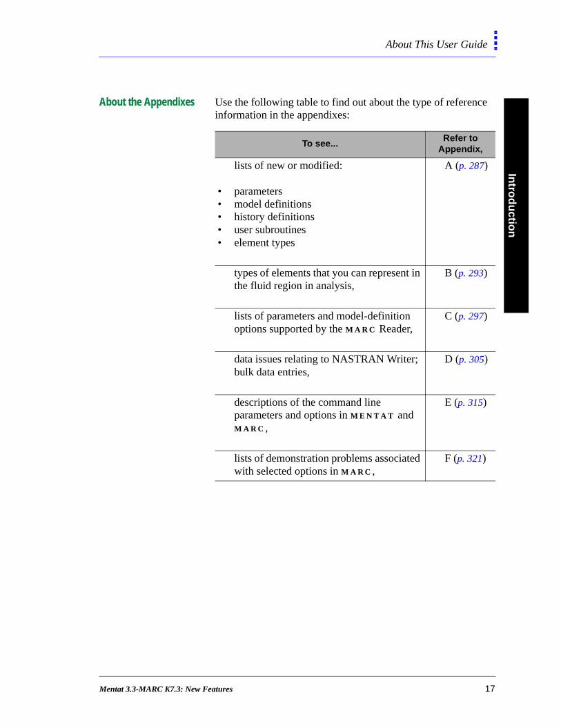
About the Appendixes Use the following table to find out about the type of reference information in the appendixes:
To see...Refer to
Appendix,
lists of new or modified:
• parameters• model definitions• history definitions• user subroutines• element types
A (p. 287)
types of elements that you can represent in the fluid region in analysis,
B (p. 293)
lists of parameters and model-definition options supported by the M A R C Reader,
C (p. 297)
data issues relating to NASTRAN Writer; bulk data entries,
D (p. 305)
descriptions of the command line parameters and options in M E N T A T and M A R C ,
E (p. 315)
lists of demonstration problems associated with selected options in M A R C ,
F (p. 321)
Mentat 3.3-MARC K7.3: New Features 17
Intr
od
uct
ion
About This User Guide
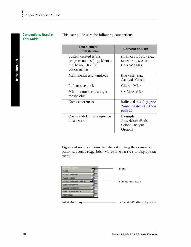
Conventions Used in This Guide
This user guide uses the following conventions:
Figures of menus contain the labels depicting the command/ button sequence (e.g., Jobs>More) in M E N T A T to display that menu.
Text element in this guide...
Convention used
System-related terms; program names (e.g., Mentat 3.3, MARC K7.3);button names
small caps, bold (e.g., M E N T A T , M A R C ; L O A D C A S E )
Main menus and windows title case (e.g., Analysis Class)
Left-mouse click Click; <ML>
Middle mouse click; right mouse click
<MM>;<MR>
Cross-references italicized text (e.g., See “Running Mentat 3.3” on page 25)
Command/ Button sequence in M E N T A T
Example: Jobs>More>Fluid-Solid>Analysis Options
Jobs>More
menu
command/button sequence
command/button
18 Mentat 3.3-MARC K7.3: New Features

Intro
du
ction
About This User Guide
Questions or Comments
For questions or comments about this guide, contact:
Technical PublicationsMARC Analysis Research Corporation260 Sheridan Avenue, Suite 309Palo Alto, CA 94306, USATel: 1 650 329 6800Fax: 1 650 323 5892
E-mail: [email protected]
Mentat 3.3-MARC K7.3: New Features 19
Intr
od
uct
ion
Supporting Documentation
of a.
Supporting Documentation
In addition to this user guide, both Mentat 3.3 and MARC K7.3 feature a variety of documentation designed for a range of user levels—beginning to advanced. For your convenience, somethese documents are available in both online and print medi
About Printed Documentation for Mentat 3.3
Use the following table to locate additional Mentat 3.3 documents that address your specific needs:
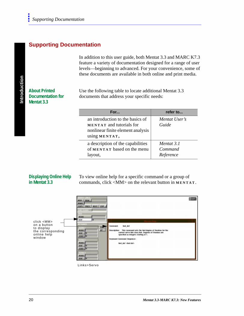
Displaying Online Help in Mentat 3.3
To view online help for a specific command or a group of commands, click <MM> on the relevant button in M E N T A T .
For... refer to...
an introduction to the basics of M E N T A T and tutorials for nonlinear finite element analysis using M E N T A T ,
Mentat User’s Guide
a description of the capabilities of M E N T A T based on the menu layout,
Mentat 3.1 Command Reference
Links>Servo L inks
cl ick <MM>on a buttonto d isp laythe correspondingonl ine helpwindow
Links>Servo
20 Mentat 3.3-MARC K7.3: New Features

Intro
du
ction
Supporting Documentation
Printed and Online Documentation for MARC K7.3
Volumes A, B, C, and D contain the documentation for MARC K7.3. These volumes are all available online or in print. To view the volumes online, refer to your CD-documentation instructions.
Use the following table to locate additional MARC K7.3 documents that address your specific needs:
Periodic Updates for Mentat 3.3 and MARC K7.3 Documentation
For periodic updates on our tutorials and documentation, choose the Tutorials/Docs link in our homepage at the following website:
http://www.marc.com
For... refer to...
background information on the capabilities of M A R C ,
Volume A: Theory and User Information
description of elements in the library and the data necessary to use them,
Volume B: Element Library
instructions on the file format of the M A R C input file,
Volume C: Program Input
description of user subroutines, Volume D: User Subroutines/Special Routines
demonstration problems for the illustration of additional analysis capabilities of M A R C
Volume E: Demonstration Problems
Mentat 3.3-MARC K7.3: New Features 21

Mentat 3.3-MARC K7.3: New Features
2• Getting Started
Running Mentat 3.3
Running Mentat 3.3 at the Command Line 25
Running MARC K7.3
About Shell Scripts 26Submitting a Job in MARC 26
Understanding the Mentat 3.3 Menu System
Setting Stand-Alone Static Menus 30Using the Root Window for Parenting 31
Dynamic Viewing
Moving an Object or a Model 33About Dynamic Viewing Options 34
Mentat 3.3-MARC K7.3: New Features 23

• Getting Started
Mentat 3.3-MARC K7.3: New Features
Gettin
g S
tartedRunning Mentat 3.3
e
Running Mentat 3.3
Running Mentat 3.3 at the Command Line
After you have installed M E N T A T on your workstation, you can run M E N T A T by typing either of the following at the command line:
• mentat
• mentat -(command line parameter)
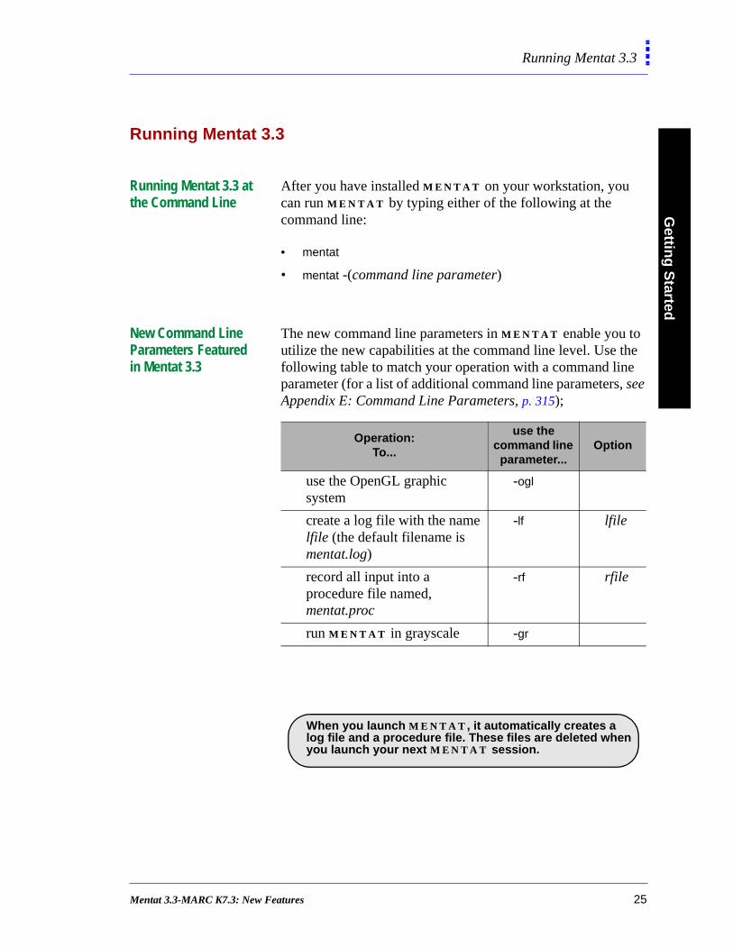
New Command Line Parameters Featured in Mentat 3.3
The new command line parameters in M E N T A T enable you to utilize the new capabilities at the command line level. Use thfollowing table to match your operation with a command lineparameter (for a list of additional command line parameters, see Appendix E: Command Line Parameters, p. 315);
Operation: To...
use the command line parameter...
Option
use the OpenGL graphic system
-ogl
create a log file with the name lfile (the default filename is mentat.log)
-lf lfile
record all input into a procedure file named, mentat.proc
-rf rfile
run M E N T A T in grayscale -gr
. When you launch M E N T A T , it automatically creates a log file and a procedure file. These files are deleted whenyou launch your next M E N T A T session.
Mentat 3.3-MARC K7.3: New Features 25
Get
tin
g S
tart
edRunning MARC K7.3
Running MARC K7.3
About Shell Scripts M A R C uses shell scripts to run machine-dependent controls or command statements. The shell script submits a job and automatically takes care of all file assignments. You must execute the shell script in the directory where all the input and output files for the M A R C job are available.
You should also ensure that every M A R C job has a unique name qualifier and that all M A R C output files connected to that job use this same qualifier. Use the default M A R C FORTRAN units for restart, post, and change state.
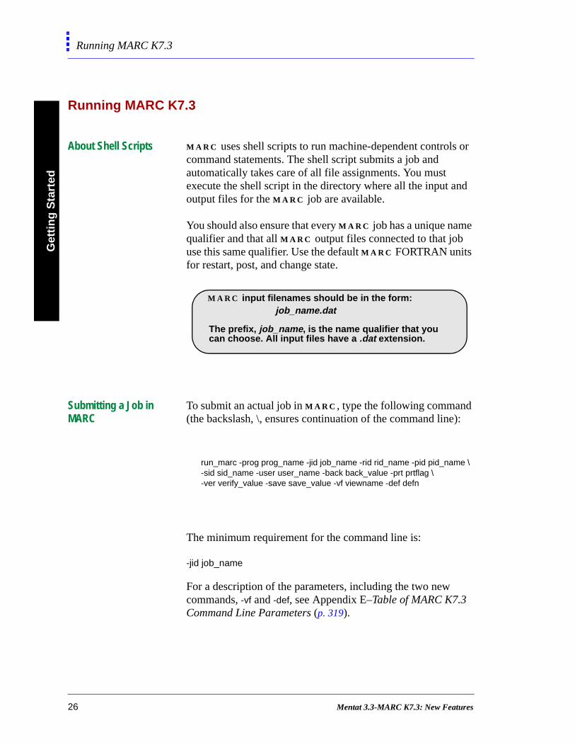
Submitting a Job in MARC
To submit an actual job in M A R C , type the following command (the backslash, \, ensures continuation of the command line):
The minimum requirement for the command line is:
-jid job_name
For a description of the parameters, including the two new commands, -vf and -def, see Appendix E–Table of MARC K7.3 Command Line Parameters (p. 319).
.
M A R C input filenames should be in the form:
job_name.dat
The prefix, job_name, is the name qualifier that you can choose. All input files have a .dat extension.
run_marc -prog prog_name -jid job_name -rid rid_name -pid pid_name \-sid sid_name -user user_name -back back_value -prt prtflag \-ver verify_value -save save_value -vf viewname -def defn
26 Mentat 3.3-MARC K7.3: New Features

Gettin
g S
tartedRunning MARC K7.3
Additional Information Use the following table to find more information:
For...refer to the Chapter... in...
installation instructions for Mentat 3.3
RunningMentat
Mentat 3.3 Installation Guide
installation instructions for MARC K7.3
Running MARC
MARC K7.3 Installation Guide
a description of how to execute MARC K7.3 on your computer
Chapter 2–Program Initiation
Vol. A
description of commands and options
Chapter 2–Program Initiation
Vol. A
description of commands and options with examples of valid input
Running MARC
MARC K7.3 Installation Guide
Mentat 3.3-MARC K7.3: New Features 27

Get
tin
g S
tart
edUnderstanding the Mentat 3.3 Menu System
e
s,
s
any
er
ent.
Understanding the Mentat 3.3 Menu System
About Enhancements in the Mentat 3.3 Menus
Here are some of the key enhancements to the Mentat 3.3 menu system:
• Menu File is simpler and easier to use; you can customiz
using the Window Parenting feature (See “Using the Root
Window for Parenting” on page 31).
• At any time during a M E N T A T session, you can resize the
selected windows dynamically (See “Resizing a Mentat 3.3
Window” on page 29).
• Procedure file, containing a record of all of your command
is created automatically (See “New Command Line Parameter
Featured in Mentat 3.3” on page 25); the default filename is
mentat.proc.
• Log file, containing diagnostics that M E N T A T reports in
the scroll area, is created automatically; you can use it in
situations such as, checking geometry surfaces, where m
messages may appear (See “New Command Line Parameters
Featured in Mentat 3.3” on page 25); the default filename is
mentat.log.
• Menu system is faster as the menu area is selectively
redrawn.
• Menu buttons are highlighted as you move the cursor ov
them.
• You can create stand-alone static menus that are perman
28 Mentat 3.3-MARC K7.3: New Features
Gettin
g S
tartedUnderstanding the Mentat 3.3 Menu System
w
d
P-
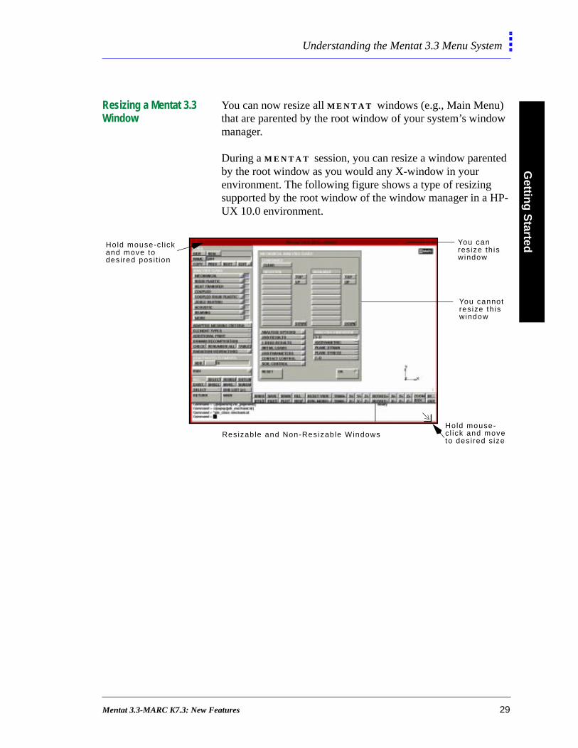
Resizing a Mentat 3.3 Window
You can now resize all M E N T A T windows (e.g., Main Menu) that are parented by the root window of your system’s windomanager.
During a M E N T A T session, you can resize a window parenteby the root window as you would any X-window in your environment. The following figure shows a type of resizing supported by the root window of the window manager in a HUX 10.0 environment.
You canresize th iswindow
You cannotres ize this window
Hold mouse-c l ick and moveto desired s ize
Hold mouse-c l ickand move todesired pos i t ion
Resizable and Non-Resizable Windows
Mentat 3.3-MARC K7.3: New Features 29
Get
tin
g S
tart
edUnderstanding the Mentat 3.3 Menu System
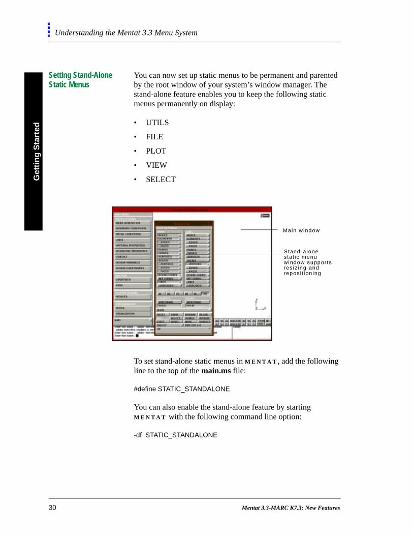
Setting Stand-Alone Static Menus
You can now set up static menus to be permanent and parented by the root window of your system’s window manager. The stand-alone feature enables you to keep the following staticmenus permanently on display:
• UTILS
• FILE
• PLOT
• VIEW
• SELECT
To set stand-alone static menus in M E N T A T , add the following line to the top of the main.ms file:
#define STATIC_STANDALONE
You can also enable the stand-alone feature by starting M E N T A T with the following command line option:
-df STATIC_STANDALONE
Main window
Stand-a lone stat ic menuwindow suppor tsres iz ing andreposit ion ing
30 Mentat 3.3-MARC K7.3: New Features

Gettin
g S
tartedUnderstanding the Mentat 3.3 Menu System
s,
,
Using the Root Window for Parenting
All M E N T A T menus and pop-ups appear in windows. The windows are parented by either the root window of your system’s window manager or the main M E N T A T window.
Windows that are parented by the root window of the windowmanager contain the window manager attributes: resizable borders, window manager menu, iconify or maximize buttonand title.
You can set a window to be parented by the root window system. The window then has the typical attributes (windowmanager borders and options, iconize and minimize buttonsetc.) of a window that is parented by a root window.
Parent ing of Windows in Mentat 3 .3
windowparented bythe rootwindow
window parented bythe mainMENTAT window
Mentat 3.3-MARC K7.3: New Features 31
Get
tin
g S
tart
edUnderstanding the Mentat 3.3 Menu System
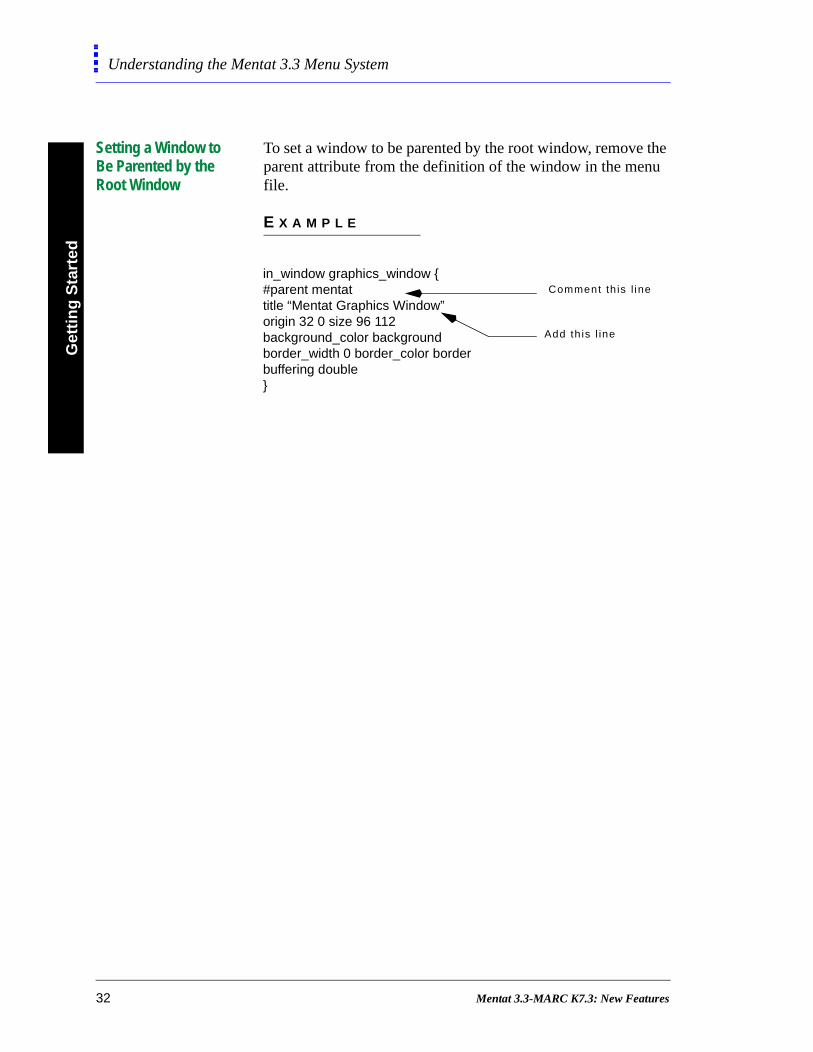
Setting a Window to Be Parented by the Root Window
To set a window to be parented by the root window, remove the parent attribute from the definition of the window in the menu file.
E X A M P L E
in_window graphics_window {#parent mentattitle “Mentat Graphics Window”origin 32 0 size 96 112background_color backgroundborder_width 0 border_color borderbuffering double}
Comment th is l ine
Add th is l ine
32 Mentat 3.3-MARC K7.3: New Features
Gettin
g S
tartedDynamic Viewing
Dynamic Viewing
About the Dynamic Viewing Feature
The Dynamic Viewing feature enables you to control the movement of the model with respect to the screen using the mouse. The Dynamic Viewing feature in Mentat 3.3 supports more keyboard and mouse options than earlier versions of M E N T A T .
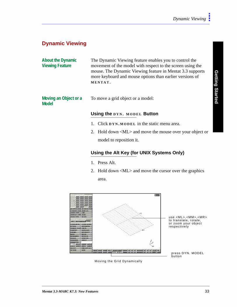
Moving an Object or a Model
To move a grid object or a model:
Using the D Y N . M O D E L Button
1. Click D Y N . M O D E L in the static menu area.
2. Hold down <ML> and move the mouse over your object or
model to reposition it.
Using the Alt Key (for UNIX Systems Only)
1. Press Alt.
2. Hold down <ML> and move the cursor over the graphics
area.
Moving the Gr id Dynamical ly
use <ML>,<MM>,<MR>to t ranslate, rotate,or zoom your ob jectrespect ive ly
press DYN. MODELbutton
Mentat 3.3-MARC K7.3: New Features 33
Get
tin
g S
tart
edDynamic Viewing
a.
ea.
About Dynamic Viewing Options
You can activate the dynamic viewing feature by choosing D Y N . M O D E L in the static menu area. After you activate the dynamic viewing feature, these are your viewing options:
• Translate
• Rotate
• Zoom In
Translating a View To translate a view:
1. Click D Y N . M O D E L .
2. Hold down <ML> and move the cursor in the graphics are
Rotating a View To rotate a view (the rotating behavior is similar to that of a space-ball device):
1. Click D Y N . M O D E L .
2. Hold down <MM> and move the cursor in the graphics
area.
Zooming a View In To zoom a view in:
1. Click D Y N . M O D E L .
2. Hold down <MR> and move the cursor in the graphics ar
34 Mentat 3.3-MARC K7.3: New Features

Gettin
g S
tartedDynamic Viewing
Additional Information Use the following table to find more information:
For...refer to the Chapter... in...
an introduction to the M E N T A T environment
Mechanics of Mentat
Mentat User’s Guide
Mentat 3.3-MARC K7.3: New Features 35

Mentat 3.3-MARC K7.3: New Features
3• Basic Procedures
File Browser
About the File Browser 39
Import-Export Utilities
About the Import Feature 42
Adaptive Plotting
About Adaptive Plotting 52
View Snapshot
About View Snapshot 57
PostScript Image Files
About the Resolution of PostScript Images 64
Arrow Settings
About Arrow Settings 68
Element Extrapolation
About Element Extrapolation for Display Purposes 71
Mentat 3.3-MARC K7.3: New Features 37

• Basic Procedures
Mentat 3.3-MARC K7.3: New Features
Basic P
roced
ures
File Browser
File Browser
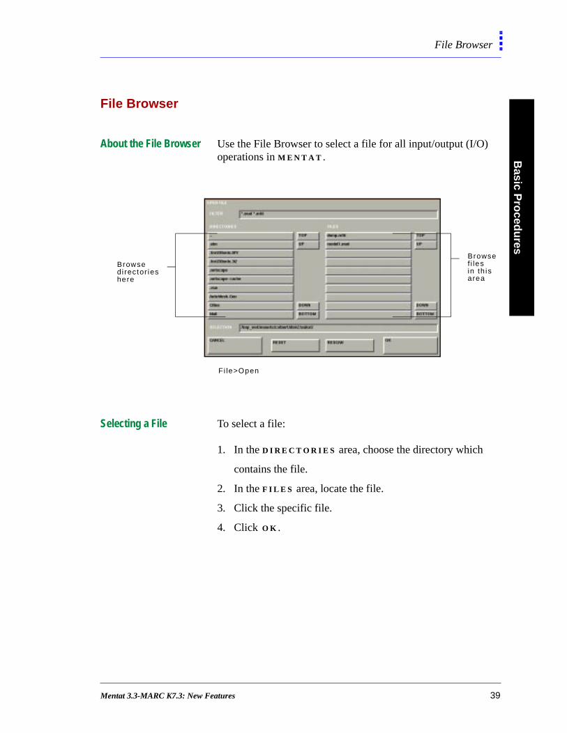
About the File Browser Use the File Browser to select a file for all input/output (I/O) operations in M E N T A T .
Selecting a File To select a file:
1. In the D I R E C T O R I E S area, choose the directory which
contains the file.
2. In the F I L E S area, locate the file.
3. Click the specific file.
4. Click O K .
Fi le>Open
Browsef i lesin th isarea
Browsedi rector ieshere
Mentat 3.3-MARC K7.3: New Features 39

Bas
ic P
roce
du
res
File Browser
Selecting a File with a Name and Location
To select a file when you know the name and location of the directory and the file:
1. In the S E L E C T I O N field, type in the name and location
(pathname) of the directory and file.
2. Press Enter.
3. Click O K .
40 Mentat 3.3-MARC K7.3: New Features
Basic P
roced
ures
File Browser
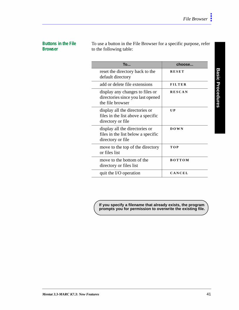
Buttons in the File Browser
To use a button in the File Browser for a specific purpose, refer to the following table:
To... choose...
reset the directory back to the default directory
R E S E T
add or delete file extensions F I L T E R
display any changes to files or directories since you last opened the file browser
R E S C A N
display all the directories or files in the list above a specific directory or file
U P
display all the directories or files in the list below a specific directory or file
D O W N
move to the top of the directory or files list
T O P
move to the bottom of the directory or files list
B O T T O M
quit the I/O operation C A N C E L
. If you specify a filename that already exists, the program prompts you for permission to overwrite the existing file.
Mentat 3.3-MARC K7.3: New Features 41

Bas
ic P
roce
du
res
Import-Export Utility
Import-Export Utility
About the Import Feature
Use the Import feature to translate the following data types into M E N T A T :
• ACIS
• DXF
• I-DEAS
• IGES
• NASTRAN
• PATRAN
• VDAFS
• MARC Input
Use the Import menu in M E N T A T to translate the data types.
Fi les>Fi le I /O>Import
42 Mentat 3.3-MARC K7.3: New Features

Basic P
roced
ures
Import-Export Utility
s,
About the Export Feature
Use the Export feature to create the following data types in Mentat:
• ACIS
• IGES
• FIDAP
• NASTRAN
Use the Export menu in M E N T A T to create the above data types.
Importing an ACIS File To import an ACIS file:
1. Choose Files>Import.
2. Choose B I N A R Y or T E X T .
3. Click A C I S .
4. Using the file browser, choose the ACIS file.
5. Click O K .
The ACIS file that you read in comprises of a number of solideach consisting of solids, faces, edges, and vertices.
Fi les>Fi le I /O>Export
. ACIS binary files have .sab extension. ACIS text files
have a .sat extension.
Mentat 3.3-MARC K7.3: New Features 43
Bas
ic P
roce
du
res
Import-Export Utility
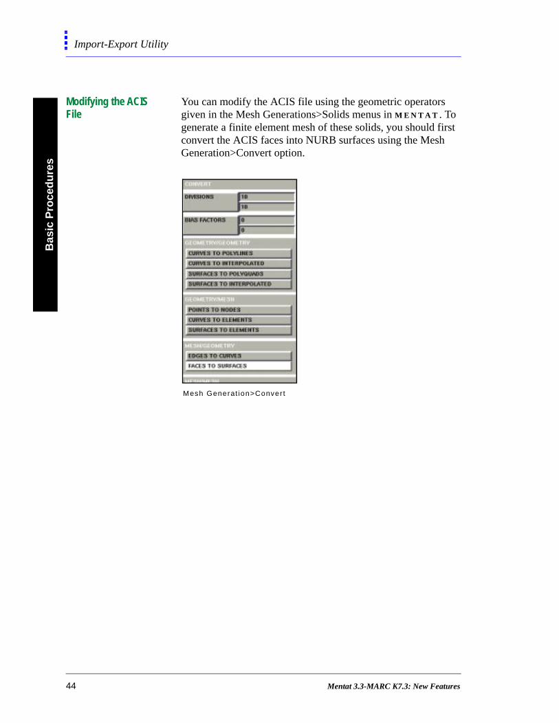
Modifying the ACIS File
You can modify the ACIS file using the geometric operators given in the Mesh Generations>Solids menus in M E N T A T . To generate a finite element mesh of these solids, you should first convert the ACIS faces into NURB surfaces using the Mesh Generation>Convert option.
Mesh Generat ion>Conver t
44 Mentat 3.3-MARC K7.3: New Features
Basic P
roced
ures
Import-Export Utility
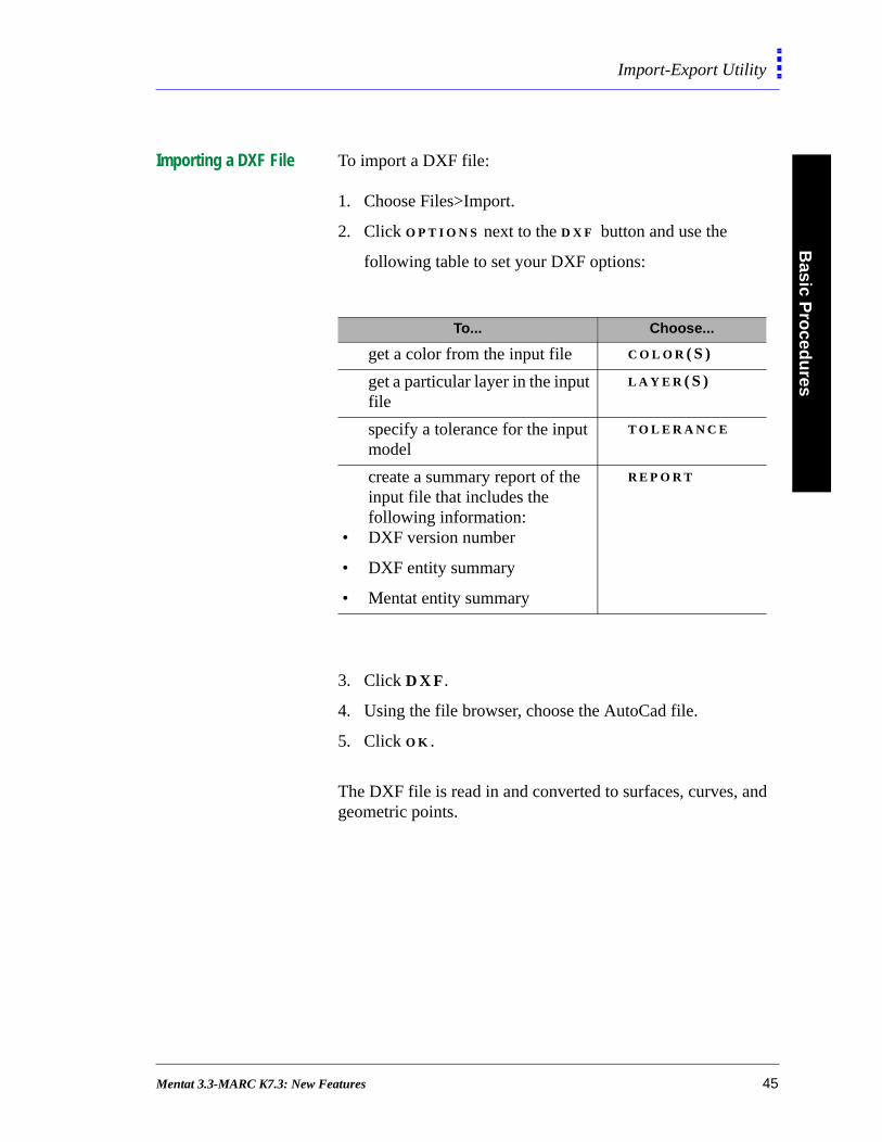
Importing a DXF File To import a DXF file:
1. Choose Files>Import.
2. Click O P T I O N S next to the D X F button and use the
following table to set your DXF options:
3. Click D X F.
4. Using the file browser, choose the AutoCad file.
5. Click O K .
The DXF file is read in and converted to surfaces, curves, and geometric points.
To... Choose...
get a color from the input file C O L O R ( S )
get a particular layer in the input file
L A Y E R ( S )
specify a tolerance for the input model
T O L E R A N C E
create a summary report of the input file that includes the following information:
• DXF version number
• DXF entity summary
• Mentat entity summary
R E P O R T
Mentat 3.3-MARC K7.3: New Features 45

Bas
ic P
roce
du
res
Import-Export Utility
Importing an I-DEAS File
To import an I-DEAS file:
1. Choose Files>Import.
2. Click I - D E A S .
3. Using the file browser, choose the I-DEAS file.
4. Click O K .
The I-DEAS universal file is read in and the finite element model will be updated to contain the model, boundary conditions and material properties from the SDRC model.
46 Mentat 3.3-MARC K7.3: New Features

Basic P
roced
ures
Import-Export Utility
Importing an IGES File To import an IGES file:
1. Choose Files>Import.
2. Click O P T I O N S and use the following table to set your
IGES options:
3. Click I G E S .
4. Using the file browser, choose the IGES file.
5. Click O K .
To... Choose...
• turn on validation of IGES entities
• correct invalid entities so that they
can be processed
• check explicitly-defined semantics
in the IGES specification
V A L I D A T E ( O N )
include model space curves from the IGES files in the Mentat model
R E A L S P C R V ( O N )
get a color from the input file C O L O R ( S )
get a particular level in the input file
L E V E L ( S )
specify a tolerance for the input model
T O L E R A N C E
create a summary report of the input file that includes the following information:
• IGES version number
• IGES entity summary
• Mentat entity summary
R E P O R T
Mentat 3.3-MARC K7.3: New Features 47

Bas
ic P
roce
du
res
Import-Export Utility
The IGES file is read in and the geometric entities are converted to surfaces, curves, and points. Finite element entities are converted to equivalent M E N T A T element types.
Importing a NASTRAN or a PATRAN File
To import a NASTRAN or a PATRAN file:
1. Choose Files>Import.
2. Choose N A S T R A N or P A T R A N .
3. Using the file browser, choose a NASTRAN or a PATRAN
file.
4. Click O K .
The finite element data is merged into the M E N T A T model.
48 Mentat 3.3-MARC K7.3: New Features
Basic P
roced
ures
Import-Export Utility
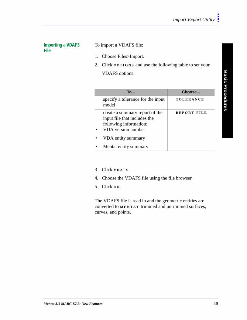
Importing a VDAFS File
To import a VDAFS file:
1. Choose Files>Import.
2. Click O P T I O N S and use the following table to set your
VDAFS options:
3. Click V D A F S .
4. Choose the VDAFS file using the file browser.
5. Click O K .
The VDAFS file is read in and the geometric entities are converted to M E N T A T trimmed and untrimmed surfaces, curves, and points.
To... Choose...
specify a tolerance for the input model
T O L E R A N C E
create a summary report of the input file that includes the following information:
• VDA version number
• VDA entity summary
• Mentat entity summary
R E P O R T F I L E
Mentat 3.3-MARC K7.3: New Features 49
Bas
ic P
roce
du
res
Import-Export Utility
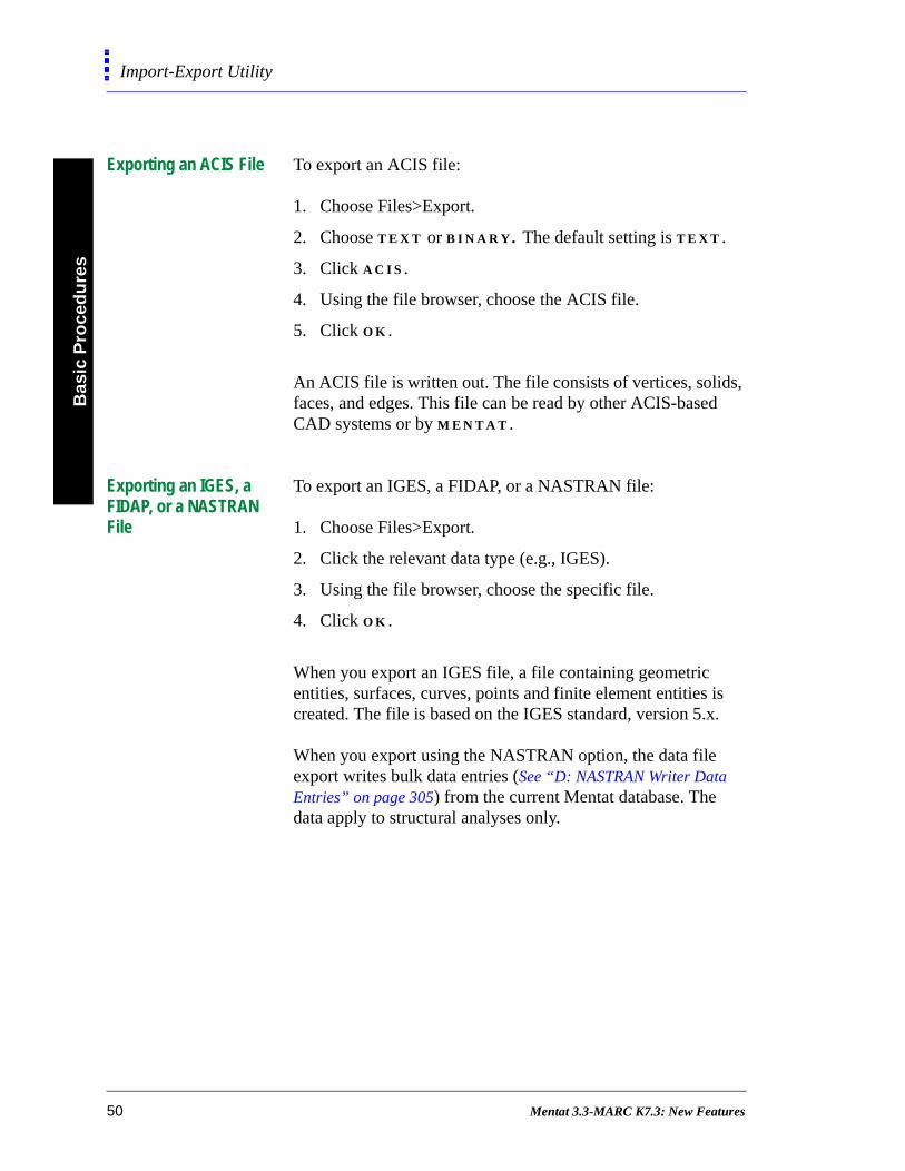
Exporting an ACIS File To export an ACIS file:
1. Choose Files>Export.
2. Choose T E X T or B I N A R Y. The default setting is T E X T .
3. Click A C I S .
4. Using the file browser, choose the ACIS file.
5. Click O K .
An ACIS file is written out. The file consists of vertices, solids, faces, and edges. This file can be read by other ACIS-based CAD systems or by M E N T A T .
Exporting an IGES, a FIDAP, or a NASTRAN File
To export an IGES, a FIDAP, or a NASTRAN file:
1. Choose Files>Export.
2. Click the relevant data type (e.g., IGES).
3. Using the file browser, choose the specific file.
4. Click O K .
When you export an IGES file, a file containing geometric entities, surfaces, curves, points and finite element entities is created. The file is based on the IGES standard, version 5.x.
When you export using the NASTRAN option, the data file export writes bulk data entries (See “D: NASTRAN Writer Data Entries” on page 305) from the current Mentat database. The data apply to structural analyses only.
50 Mentat 3.3-MARC K7.3: New Features

Basic P
roced
ures
Import-Export Utility
Importing a MARC Data File
You can read in and merge existing M A R C files with the current model in M E N T A T . A stand-alone program, based on M A R C , reads the parameter and model definition data only and prevents the inclusion of bad incrementation data in the model. For a list of stored data types, see Appendix C: MARC Data Reader Support (p. 297).
To import a M A R C data file:
1. Choose FIles>Read.
2. Choose the relevant file in the file browser.
3. Click O K .
Fi les
Mentat 3.3-MARC K7.3: New Features 51

Bas
ic P
roce
du
res
Adaptive Plotting
Adaptive Plotting
About Adaptive Plotting
The adaptive plotting feature automatically changes the number of divisions used to represent curves or surfaces based on the curvature. The feature uses more divisions in areas of high curvature which enables you to use a minimum number of graphics resources.
Based on a tolerance that you specify, the feature works identically for curves and surfaces.
Tolerance and Modes of Tolerances
The tolerance in adaptive plotting is the measure of the deviation between the curves that are drawn and the actual curve.
When you change the default tolerance settings in the adaptive plotting feature, you can choose either of the following types of tolerances:
• relative
• absolute
drawn curve
actual curve
segments drawn wi th are la t ively lower to lerance
segments drawn with arela t ive ly higher to lerance
52 Mentat 3.3-MARC K7.3: New Features
Basic P
roced
ures
Adaptive Plotting
s
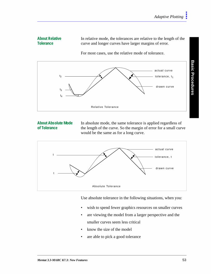
About Relative Tolerance
In relative mode, the tolerances are relative to the length of the curve and longer curves have larger margins of error.
For most cases, use the relative mode of tolerance.
About Absolute Mode of Tolerance
In absolute mode, the same tolerance is applied regardless of the length of the curve. So the margin of error for a small curve would be the same as for a long curve.
Use absolute tolerance in the following situations, when you:
• wish to spend fewer graphics resources on smaller curve
• are viewing the model from a larger perspective and the
smaller curves seem less critical
• know the size of the model
• are able to pick a good tolerance
actual curve
to lerance, t1
drawn curve
Relat ive Tolerance
t2
t3
t4
t
t
tolerance, t
drawn curve
actual curve
Absolute Tolerance
Mentat 3.3-MARC K7.3: New Features 53
Bas
ic P
roce
du
res
Adaptive Plotting
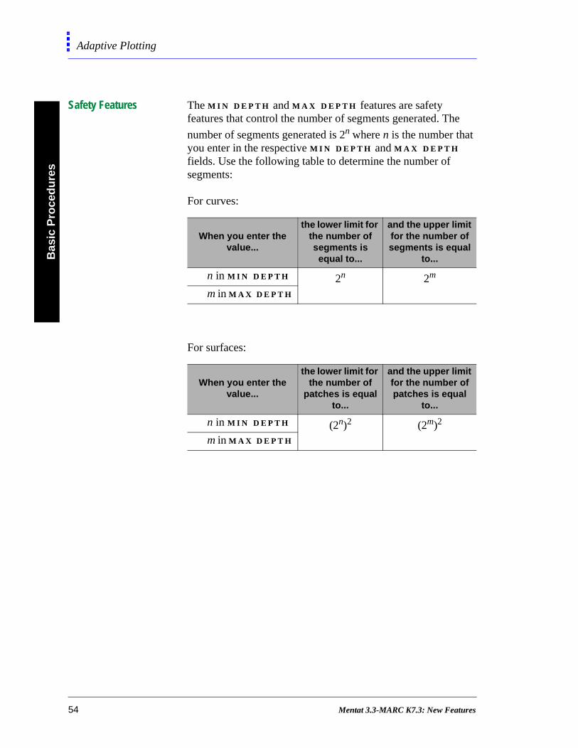
Safety Features The M I N D E P T H and M A X D E P T H features are safety features that control the number of segments generated. The
number of segments generated is 2n where n is the number that you enter in the respective M I N D E P T H and M A X D E P T H fields. Use the following table to determine the number of segments:
For curves:
For surfaces:
When you enter the value...
the lower limit for the number of segments is equal to...
and the upper limit for the number of segments is equal
to...
n in M I N D E P T H 2n 2m
m in M A X D E P T H
When you enter the value...
the lower limit for the number of
patches is equal to...
and the upper limit for the number of patches is equal
to...
n in M I N D E P T H (2n)2 (2m)2
m in M A X D E P T H
54 Mentat 3.3-MARC K7.3: New Features
Basic P
roced
ures
Adaptive Plotting
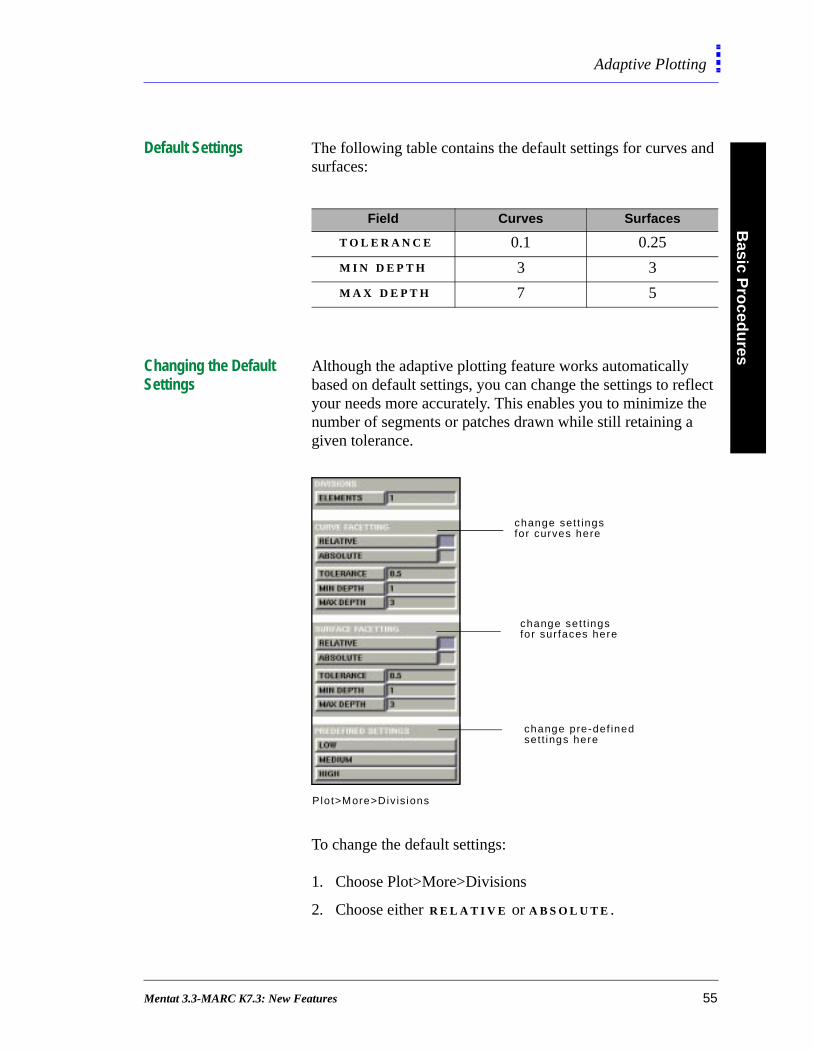
Default Settings The following table contains the default settings for curves and surfaces:
Changing the Default Settings
Although the adaptive plotting feature works automatically based on default settings, you can change the settings to reflect your needs more accurately. This enables you to minimize the number of segments or patches drawn while still retaining a given tolerance.
To change the default settings:
1. Choose Plot>More>Divisions
2. Choose either R E L A T I V E or A B S O L U T E .
Field Curves Surfaces
T O L E R A N C E 0.1 0.25
M I N D E P T H 3 3
M A X D E P T H 7 5
change set t ingsfor curves here
change set t ingsfor sur faces here
Plot>More>Div is ions
change pre-def inedsett ings here
Mentat 3.3-MARC K7.3: New Features 55
Bas
ic P
roce
du
res
Adaptive Plotting
e
e p
3. Choose one of the following options:
• To change the settings for curves, choose C U R V E
F A C E T T I N G .
• To change the settings for surfaces, choose S U R F A C E
F A C E T T I N G .
4. Click T O L E R A N C E and type in a value.
5. Click M I N D E P T H and type in a value.
6. Click M A X D E P T H and type in a value.
About Pre-Defined Settings
Depending on the degree of accuracy of plotting that you araiming for, you can choose from among the following pre-defined settings:
• high
• medium
• low
Use the “high” setting when the accuracy of the plotting of surfaces and curves is critical. Use the “low” setting when thaccuracy of plotting is not so critical and you wish to speed uthe display of the model.
Additional Information Use the following table to find more information:
For...refer to
Chapter(s)...in...
description of buttons in the Adaptive Plotting menus
15:Visualization Mentat 3.1 Command Reference
56 Mentat 3.3-MARC K7.3: New Features
Basic P
roced
ures
View Snapshot
t.
to.
View Snapshot
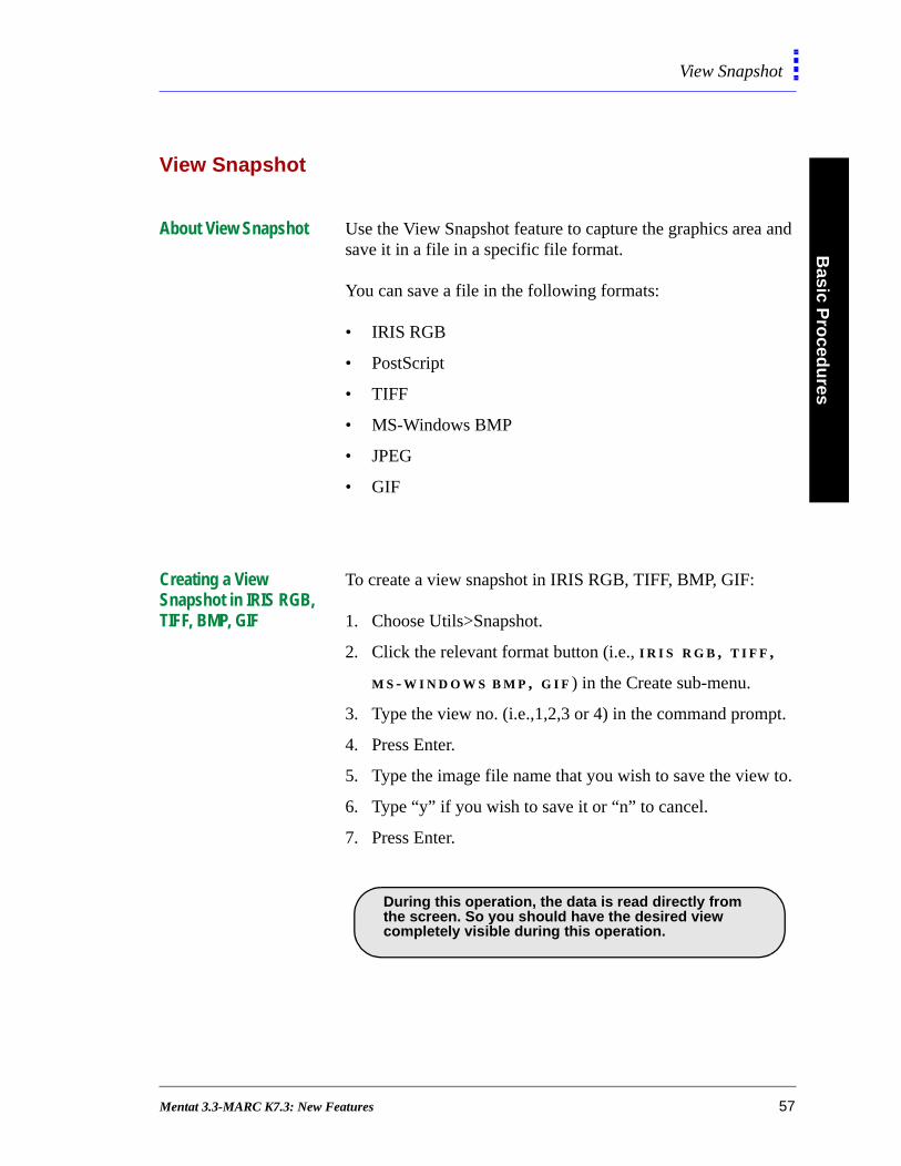
About View Snapshot Use the View Snapshot feature to capture the graphics area and save it in a file in a specific file format.
You can save a file in the following formats:
• IRIS RGB
• PostScript
• TIFF
• MS-Windows BMP
• JPEG
• GIF
Creating a View Snapshot in IRIS RGB, TIFF, BMP, GIF
To create a view snapshot in IRIS RGB, TIFF, BMP, GIF:
1. Choose Utils>Snapshot.
2. Click the relevant format button (i.e., I R I S R G B , T I F F ,
M S - W I N D O W S B M P , G I F ) in the Create sub-menu.
3. Type the view no. (i.e.,1,2,3 or 4) in the command promp
4. Press Enter.
5. Type the image file name that you wish to save the view
6. Type “y” if you wish to save it or “n” to cancel.
7. Press Enter.
.
During this operation, the data is read directly from the screen. So you should have the desired view completely visible during this operation.
Mentat 3.3-MARC K7.3: New Features 57
Bas
ic P
roce
du
res
View Snapshot
PostScript Files
Creating a view snapshot in PostScript involves the following stages:
• Setting the PostScript plotting attributes
• Creating the view snapshot file
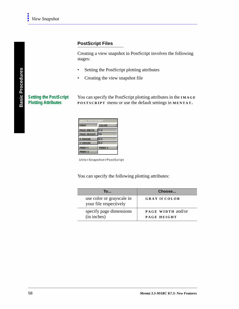
Setting the PostScript Plotting Attributes
You can specify the PostScript plotting attributes in the I M A G E P O S T S C R I P T menu or use the default settings in M E N T A T .
You can specify the following plotting attributes:
Uti ls>Snapshot>PostScr ipt
To... Choose...
use color or grayscale in your file respectively
G R A Y or C O L O R
specify page dimensions (in inches)
P A G E W I D T H and/or P A G E H E I G H T
58 Mentat 3.3-MARC K7.3: New Features
Basic P
roced
ures
View Snapshot
Creating View Snapshots in PostScript
To create view snapshots in PostScript:
1. Click U T I L I T I E S in the static menu area.
2. Click S N A P S H O T in the U T I L I T I E S menu.
3. Click P O S T S C R I P T in the C R E A T E sub-menu.
4. Type the view no. (i.e.,1,2,3 or 4) in the command prompt.
5. Press Enter.
6. Type the image file name that you wish to save the view to.
7. Type “y” if you wish to save it or “n” to cancel.
8. Press Enter.
JPEG Files
Creating a view snapshot in JPEG involves the following stages:
• Setting the JPEG attributes
• Creating the view snapshot file
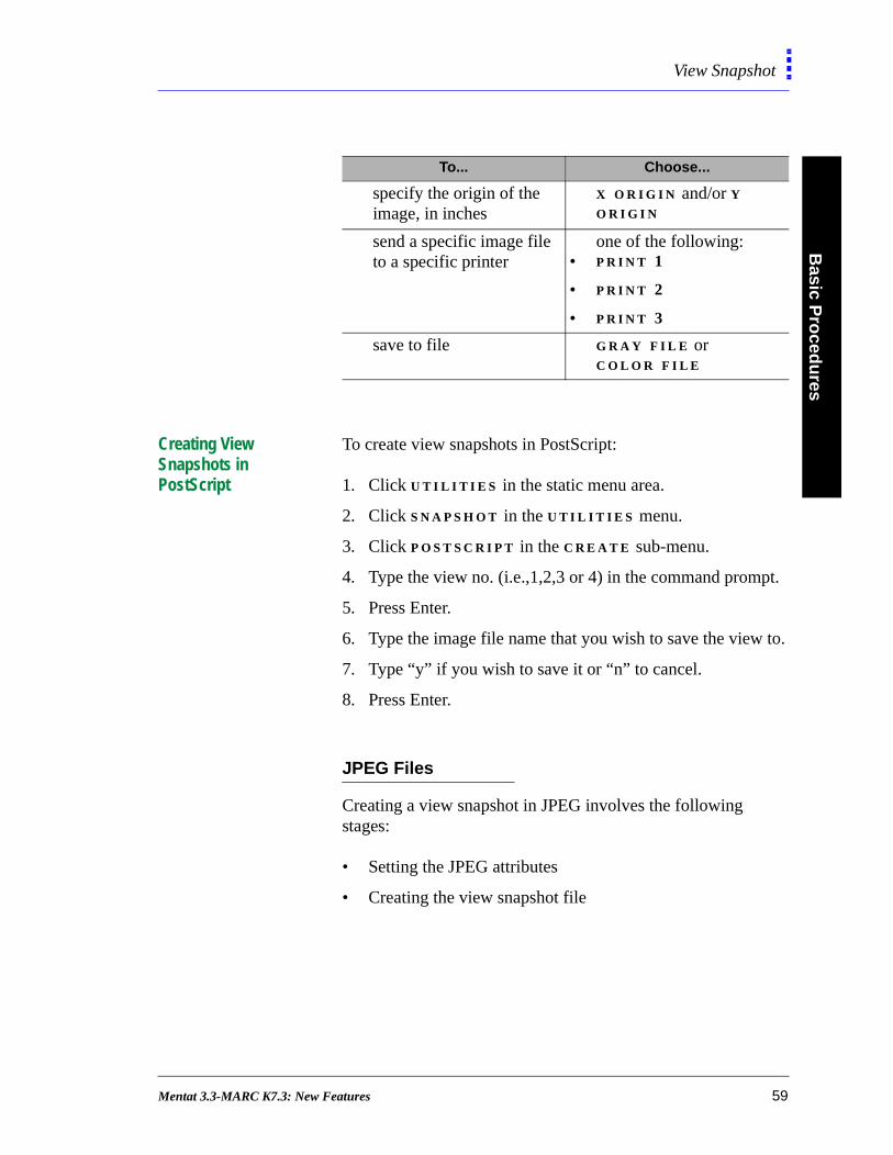
specify the origin of the image, in inches
X O R I G I N and/or Y O R I G I N
send a specific image file to a specific printer
one of the following:• P R I N T 1
• P R I N T 2
• P R I N T 3
save to file G R A Y F I L E or C O L O R F I L E
To... Choose...
Mentat 3.3-MARC K7.3: New Features 59

Bas
ic P
roce
du
res
View Snapshot
t.
Setting the JPEG Attributes
Use the following table to set the JPEG attributes:
The default attributes are:
• J P E G Q U A L I T Y —75
• J P E G S M O O T H I N G —15
Changing the Default JPEG Attributes
To change the default JPEG attributes:
1. Click J P E G Q U A L I T Y in the Attributes sub-menu.
2. Enter a new value.
3. Click J P E G S M O O T H I N G .
4. Enter a new value.
Creating View Snapshots in JPEG
To create view snapshots in JPEG:
1. Choose Utils>Snapshot.
2. Click J P E G in the C R E A T E sub-menu.
3. Type the view no. (i.e.,1,2,3 or 4) in the command promp
To set the JPEG attribute...
with a range of values...
Click...
Quality (the higher the value, the greater the file size and better the image quality)
1-100 J P E G Q U A L I T Y
Smoothing (reduces the distortion of edges when you shrink or expand an image)
5-30 J P E G S M O O T H I N G
60 Mentat 3.3-MARC K7.3: New Features

Basic P
roced
ures
View Snapshot
4. Press Enter.
5. Type the image file name that you wish to save the view to.
6. Type “y” if you wish to save it or “n” to cancel.
7. Press Enter.
Mentat 3.3-MARC K7.3: New Features 61
Bas
ic P
roce
du
res
Plotting PostScript Image Files
e
ript.
u
Plotting PostScript Image Files
About Plotting a Graphics Image
You can plot grayscale or color graphics images in M E N T A T using either of the following options:
• send a PostScript file (color or grayscale) representing th
current graphics image to a specific printer. To use this
option, you must configure the printer by editing the
appropriate file in the bin directory.
• write a PostScript output (color or grayscale) to a file.
Printing PostScript Image Files
After you write a PostScript output to a file, you can print theimage in one or more of the following ways:
• send the PostScript file to a printer that supports PostSc
• import the PostScript file as an object into an application
that reads PostScript files as input (e.g. FrameMaker).
Depending on the application, you can alter the object
attributes (e.g., size, rotation, aspect ratio, etc.) before yo
print the image.
. The image files shown here were written as
PostScript output files in M E N T A T and read into FrameMaker, a document publishing software.
62 Mentat 3.3-MARC K7.3: New Features

Basic P
roced
ures
Plotting PostScript Image Files
Setting PostScript Image File Attributes
To set the image attributes of a PostScript file before you write it to a file or a printer:
1. Click U T I L S in the static menu area.
2. Click S E T T I N G S and enter the image attributes.
Sending a PostScript Output Directly to a Printer
To send a PostScript image file directly to the printer (you must configure your printer before you send the file):
1. Click U T I L I T I E S in the static menu area.
2. Choose a printer destination (e.g., Color Print 1) for the
output file.
Ut i ls>(PostScr ip t)Sett ings
set the s ize of the
set the or igins ( in inches)
set the resolut ion of
image
the image
set the or ientat ionof the image
of the image area
Ut i l i t ies
speci fy d i fferent prin ters as dest inat ions for the output f i le
Mentat 3.3-MARC K7.3: New Features 63
Bas
ic P
roce
du
res
Plotting PostScript Image Files
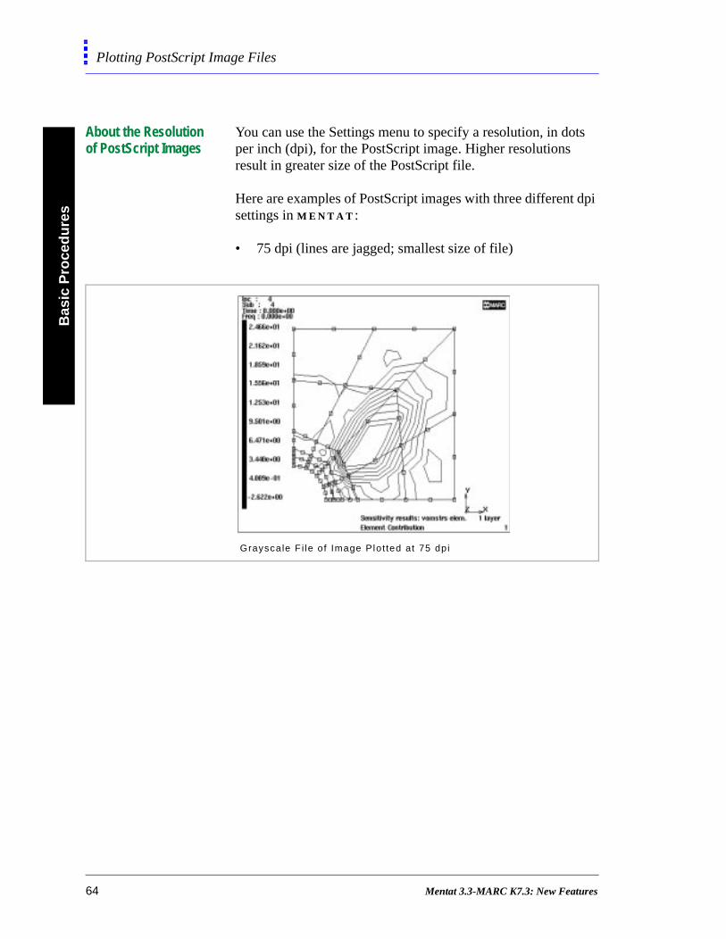
About the Resolution of PostScript Images
You can use the Settings menu to specify a resolution, in dots per inch (dpi), for the PostScript image. Higher resolutions result in greater size of the PostScript file.
Here are examples of PostScript images with three different dpi settings in M E N T A T :
• 75 dpi (lines are jagged; smallest size of file)
Grayscale F i le of Image Plot ted at 75 dpi
64 Mentat 3.3-MARC K7.3: New Features
Basic P
roced
ures
Plotting PostScript Image Files
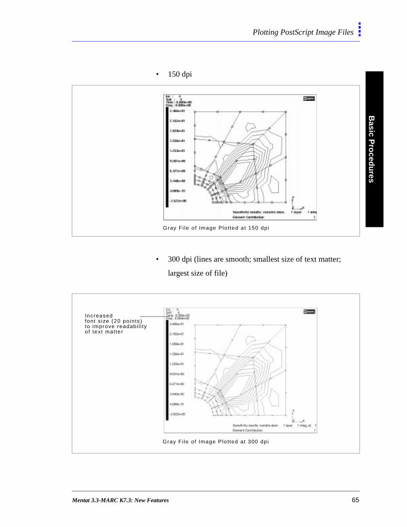
• 150 dpi
• 300 dpi (lines are smooth; smallest size of text matter;
largest size of file)
Gray Fi le o f Image Plot ted at 150 dpi
Increased font s ize (20 po ints)to improve readabi l i tyof text matter
Gray F i le of Image P lot ted at 300 dpi
Mentat 3.3-MARC K7.3: New Features 65

Bas
ic P
roce
du
res
Plotting PostScript Image Files
Increasing the Font Size of Text Matter
When you choose a higher resolution (e.g., 300 dpi) for the image, the text matter in the image area appears relatively smaller. You can offset this by increasing the font size for the text matter in the image area before you write the PostScript output file.
To increase the font size of the text matter in the image area:
1. Choose Device>Set Font.
2. From the list of available fonts, choose a larger font size
(e.g., 32).
. For quality images, choose a resolution that is higherthan 75 dpi.
l i s t o f avai lab lefonts in your loca lenv i ronmentor pla t form
Device>Set Font
. The list of available fonts and font sizes vary depending
on your local environment/platform.
66 Mentat 3.3-MARC K7.3: New Features
Basic P
roced
ures
Plotting PostScript Image Files
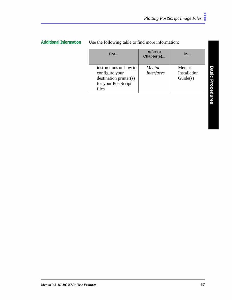
Additional Information Use the following table to find more information:
For...refer to
Chapter(s)...in...
instructions on how to configure your destination printer(s) for your PostScript files
Mentat Interfaces
Mentat Installation Guide(s)
Mentat 3.3-MARC K7.3: New Features 67

Bas
ic P
roce
du
res
Arrow Settings
Arrow Settings
About Arrow Settings Use the Arrow Settings feature to indicate boundary conditions on your finite element model. You can specify the following attributes for the arrows:
• length—for preprocessing arrows
• mode—for all arrows
To view the Arrow Settings options, choose Boundary Conditions>Arrow Settings.
Specifying the Length of Preprocessing Arrows Manually
To specify the length of preprocessing arrows in the user coordinate system manually:
1. Choose Boundary Conditions>Arrow Settings.
2. Choose M A N U A L .
3. Click L E N G T H and specify a value.
Boundary Condi t ions>Arrow Sett ings
68 Mentat 3.3-MARC K7.3: New Features

Basic P
roced
ures
Arrow Settings
n
Scaling the Length of Arrows Automatically
You can specify the length of arrows to be a percentage of the graphics screen. The arrows are then automatically scaled with respect to the graphics screen. Use the F A C T O R button to set the percentage of the graphics screen.
To scale the lengths of arrows automatically:
1. Choose Boundary Conditions>Arrow Settings.
2. Click A U T O M A T I C .
3. Click F A C T O R and enter a fraction (e.g., 0.2).
About Arrow Modes You can specify how the arrows are drawn by choosing one of the following modes:
• wireframe
• solid
Use the # F A C E T S button to specify the number of facets for aarrow.
wireframe arrow
sol id ar rows
wi th edges without edges
facet
Mentat 3.3-MARC K7.3: New Features 69

Bas
ic P
roce
du
res
Arrow Settings
Additional Information Use the following table to find more information:
For...refer to
Chapter(s)...in...
description of buttons in the Arrow Settings menu
4:Boundary Conditions–Arrow Settings
Mentat 3.1 Command Reference
70 Mentat 3.3-MARC K7.3: New Features
Basic P
roced
ures
Element Extrapolation
n
int
at
e
Element Extrapolation
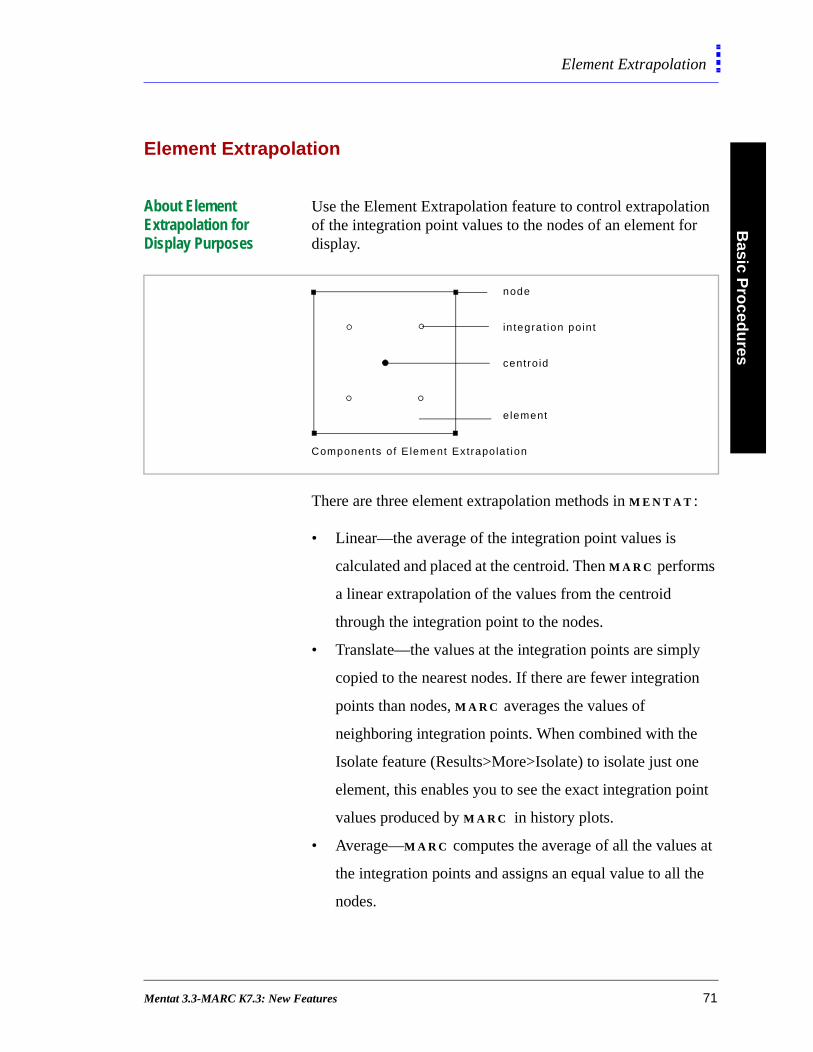
About Element Extrapolation for Display Purposes
Use the Element Extrapolation feature to control extrapolation of the integration point values to the nodes of an element for display.
There are three element extrapolation methods in M E N T A T :
• Linear—the average of the integration point values is
calculated and placed at the centroid. Then M A R C performs
a linear extrapolation of the values from the centroid
through the integration point to the nodes.
• Translate—the values at the integration points are simply
copied to the nearest nodes. If there are fewer integratio
points than nodes, M A R C averages the values of
neighboring integration points. When combined with the
Isolate feature (Results>More>Isolate) to isolate just one
element, this enables you to see the exact integration po
values produced by M A R C in history plots.
• Average—M A R C computes the average of all the values
the integration points and assigns an equal value to all th
nodes.
node
integrat ion po int
centro id
Components of E lement Extrapolat ion
element
Mentat 3.3-MARC K7.3: New Features 71

Bas
ic P
roce
du
res
Element Extrapolation
Selecting an Element Extrapolation Option
To select an element extrapolation method in M E N T A T , choose Results>Scalar Plot Settings>Extrapolation.
About Nodal Averaging
Use the Nodal Averaging feature to control the inter-element averaging of the nodal data after extrapolation. To ensure that the contour lines are continuous, choose O N .
When you choose (nodal averaging) O F F , each element is independently contoured and the contour lines are discontinuous.
Results>(Scalar Plot ) Set t ings>Ext rapolat ion
toggles the averaging of nodalva lues between elements
nodeneighbor ingelements
Nodal Averaging Enabled
. When you notice large differences between the
averaged and the non-averaged results, the analysisis probably not very accurate.
72 Mentat 3.3-MARC K7.3: New Features
4• General Technology
Using the N to 1 and N to N Options in Links
Specifying Node Lists and Node Paths
Buckle Solutions Using Lanczos Method
Adaptive Load Stepping
Extended Precision Input
Constant Dilatation
Assumed Strain
Numerical Preferences
User-Defined Post Variables
Mentat 3.3-MARC K7.3: New Features 73

• General Technology
Mentat 3.3-MARC K7.3: New Features

Gen
eral Techn
olo
gy
Using N to 1 and N to N Options in Links
Using N to 1 and N to N Options in Links
About N to 1 and N to N Options
The N to 1 and N to N options are useful when you are applying constraint equations (ties or servo links) or springs that are similar in nature. A typical application is when you are modeling generalized plane strain conditions and you want multiple nodes to move as one node.
Here are the situations where you can use these options:
• N to 1—multiple ties between N tied nodes and common
retained node(s).
• N to 1—multiple springs between N begin nodes and one
common end node.
N to 1 wi th only
1st 2nd nth
one retained node
...
N to 1 wi th tworeta ined nodes
t iednodes
reta inednodes
1st 2nd nth...
begin
1st 2nd nth
end
N to 1 mul t ip le spr ings
...
Mentat 3.3-MARC K7.3: New Features 75
Gen
eral
Tec
hn
olo
gy
Using N to 1 and N to N Options in Links
r
d
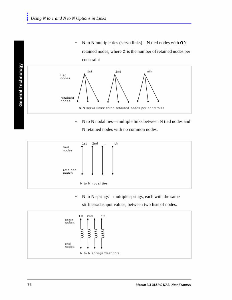
• N to N multiple ties (servo links)—N tied nodes with αN
retained nodes, where α is the number of retained nodes pe
constraint
• N to N nodal ties—multiple links between N tied nodes an
N retained nodes with no common nodes.
• N to N springs—multiple springs, each with the same
stiffness/dashpot values, between two lists of nodes.
N-N servo l inks: three reta ined nodes per const raint
1st 2nd ntht iednodes
reta inednodes
N to N nodal t ies
t iednodes
reta inednodes
1st 2nd .. . n th
N to N spr ings/dashpots
beginnodes
endnodes
1st 2nd nth. . .
76 Mentat 3.3-MARC K7.3: New Features
Gen
eral Techn
olo
gy
Using N to 1 and N to N Options in Links
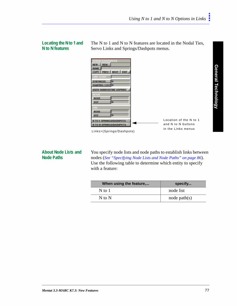
Locating the N to 1 and N to N features
The N to 1 and N to N features are located in the Nodal Ties, Servo Links and Springs/Dashpots menus.
About Node Lists and Node Paths
You specify node lists and node paths to establish links between nodes (See “Specifying Node Lists and Node Paths” on page 86). Use the following table to determine which entity to specify with a feature:
Locat ion of the N to 1and N to N buttons
in the L inks menus Links>(Spr ings/Dashpots)
When using the feature,... specify...
N to 1 node list
N to N node path(s)
Mentat 3.3-MARC K7.3: New Features 77
Gen
eral
Tec
hn
olo
gy
Using N to 1 and N to N Options in Links
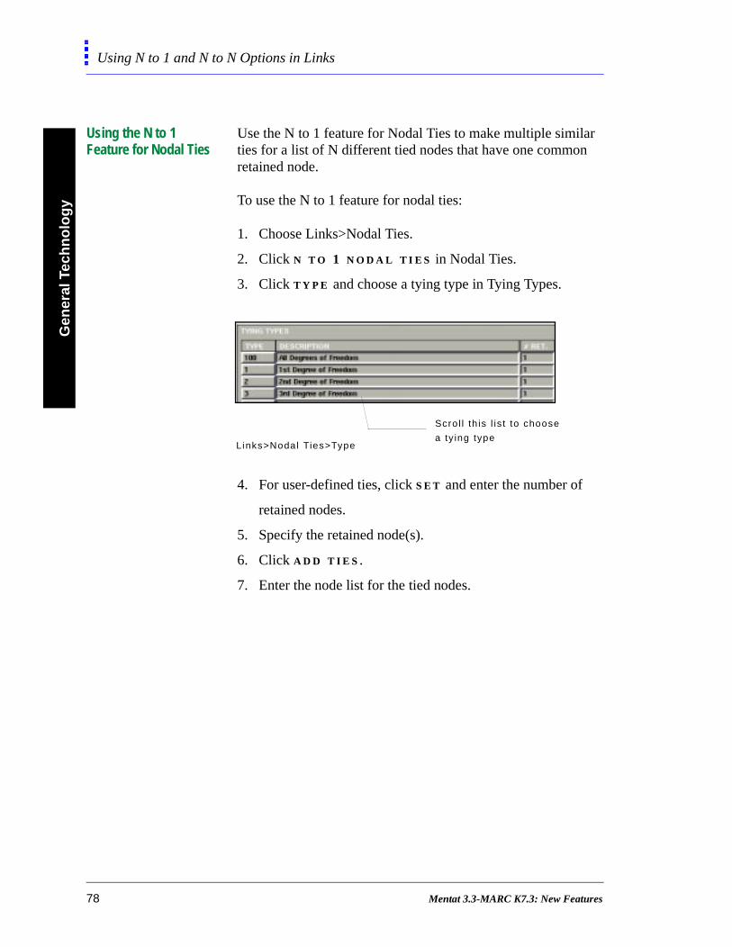
Using the N to 1 Feature for Nodal Ties
Use the N to 1 feature for Nodal Ties to make multiple similar ties for a list of N different tied nodes that have one common retained node.
To use the N to 1 feature for nodal ties:
1. Choose Links>Nodal Ties.
2. Click N T O 1 N O D A L T I E S in Nodal Ties.
3. Click T Y P E and choose a tying type in Tying Types.
4. For user-defined ties, click S E T and enter the number of
retained nodes.
5. Specify the retained node(s).
6. Click A D D T I E S .
7. Enter the node list for the tied nodes.
Scro l l th is l is t to choose
a ty ing typeLinks>Nodal Ties>Type
78 Mentat 3.3-MARC K7.3: New Features
Gen
eral Techn
olo
gy
Using N to 1 and N to N Options in Links
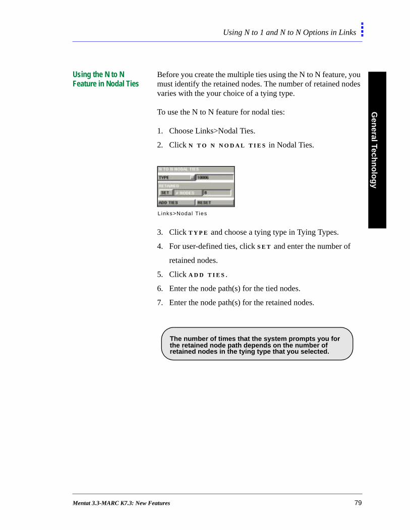
Using the N to N Feature in Nodal Ties
Before you create the multiple ties using the N to N feature, you must identify the retained nodes. The number of retained nodes varies with the your choice of a tying type.
To use the N to N feature for nodal ties:
1. Choose Links>Nodal Ties.
2. Click N T O N N O D A L T I E S in Nodal Ties.
3. Click T Y P E and choose a tying type in Tying Types.
4. For user-defined ties, click S E T and enter the number of
retained nodes.
5. Click A D D T I E S .
6. Enter the node path(s) for the tied nodes.
7. Enter the node path(s) for the retained nodes.
Links>Nodal Ties
.The number of times that the system prompts you for the retained node path depends on the number ofretained nodes in the tying type that you selected.
Mentat 3.3-MARC K7.3: New Features 79

Gen
eral
Tec
hn
olo
gy
Using N to 1 and N to N Options in Links
Using the N to 1 Feature in Servo Links
The servo link constraint is of the general form:
where is the displacement of the tied node, is the
displacement of the R1 retained node, and C1 is the corresponding coefficient.
Use the N to 1 feature in servo links to create a servo link having multiple tied nodes and one common set of retained nodes.
To use the N to 1 feature in servo links:
1. Choose Links>Servo Links.
2. Click N T O 1 S E R V O L I N K S in Servo Links.
3. Specify the degree of freedom for the tied node.
4. Enter the number of terms in the servo link equation.
5. Define the following for each term:
• retained node
• degree of freedom
• coefficient
6. Click A D D T I E S .
7. Enter the node list for the tied nodes.
UDOFT C1UDOF
R1 C2UDOFR2+=
UTDOF UDOF
R1
Links>Servo L inks>N to 1 Servo L inks
80 Mentat 3.3-MARC K7.3: New Features

Gen
eral Techn
olo
gy
Using N to 1 and N to N Options in Links
Using the N to N Feature in Servo Links
To use the N to N feature in servo links:
1. Choose Links>Servo Links.
2. Click N T O N S E R V O L I N K S in Servo Links.
3. Specify the degree of freedom for the tied node.
4. Enter the number of terms in the servo link equation.
5. Define the following for each term:
• degree of freedom
• coefficient
6. Click A D D S E R V O S .
7. Enter the node path for the tied nodes.
8. Enter the node path(s) for the tied nodes followed by the
retained nodes.
.
The number of times that the system prompts you for the retained node path depends on the number of termsthat you specify.
Mentat 3.3-MARC K7.3: New Features 81
Gen
eral
Tec
hn
olo
gy
Using N to 1 and N to N Options in Links
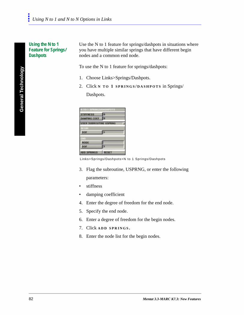
Using the N to 1 Feature for Springs/Dashpots
Use the N to 1 feature for springs/dashpots in situations where you have multiple similar springs that have different begin nodes and a common end node.
To use the N to 1 feature for springs/dashpots:
1. Choose Links>Springs/Dashpots.
2. Click N T O 1 S P R I N G S / D A S H P O T S in Springs/
Dashpots.
3. Flag the subroutine, USPRNG, or enter the following
parameters:
• stiffness
• damping coefficient
4. Enter the degree of freedom for the end node.
5. Specify the end node.
6. Enter a degree of freedom for the begin nodes.
7. Click A D D S P R I N G S .
8. Enter the node list for the begin nodes.
Links>Spr ings/Dashpots>N to 1 Spr ings/Dashpots
82 Mentat 3.3-MARC K7.3: New Features
Gen
eral Techn
olo
gy
Using N to 1 and N to N Options in Links
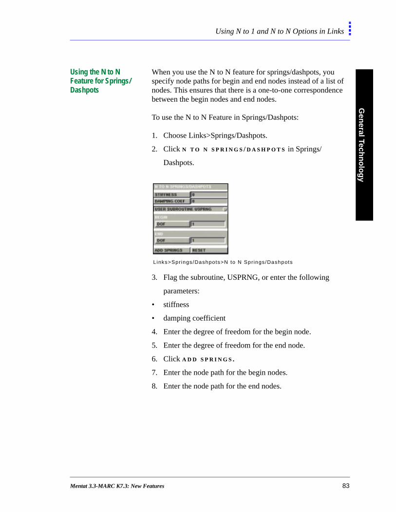
Using the N to N Feature for Springs/Dashpots
When you use the N to N feature for springs/dashpots, you specify node paths for begin and end nodes instead of a list of nodes. This ensures that there is a one-to-one correspondence between the begin nodes and end nodes.
To use the N to N Feature in Springs/Dashpots:
1. Choose Links>Springs/Dashpots.
2. Click N T O N S P R I N G S / D A S H P O T S in Springs/
Dashpots.
3. Flag the subroutine, USPRNG, or enter the following
parameters:
• stiffness
• damping coefficient
4. Enter the degree of freedom for the begin node.
5. Enter the degree of freedom for the end node.
6. Click A D D S P R I N G S .
7. Enter the node path for the begin nodes.
8. Enter the node path for the end nodes.
Links>Springs/Dashpots>N to N Spr ings/Dashpots
Mentat 3.3-MARC K7.3: New Features 83
Gen
eral
Tec
hn
olo
gy
Using N to 1 and N to N Options in Links
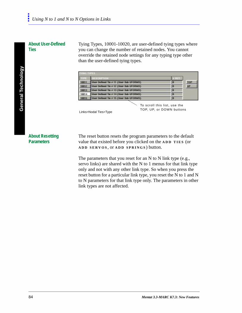
About User-Defined Ties
Tying Types, 10001-10020, are user-defined tying types where you can change the number of retained nodes. You cannot override the retained node settings for any typing type other than the user-defined tying types.
About Resetting Parameters
The reset button resets the program parameters to the default value that existed before you clicked on the A D D T I E S (or A D D S E R V O S , or A D D S P R I N G S ) button.
The parameters that you reset for an N to N link type (e.g., servo links) are shared with the N to 1 menus for that link type only and not with any other link type. So when you press the reset button for a particular link type, you reset the N to 1 and N to N parameters for that link type only. The parameters in other link types are not affected.
To scrol l this l is t , use theTOP, UP, or DOWN buttons
Links>Nodal Ties>Type
84 Mentat 3.3-MARC K7.3: New Features
Gen
eral Techn
olo
gy
Using N to 1 and N to N Options in Links
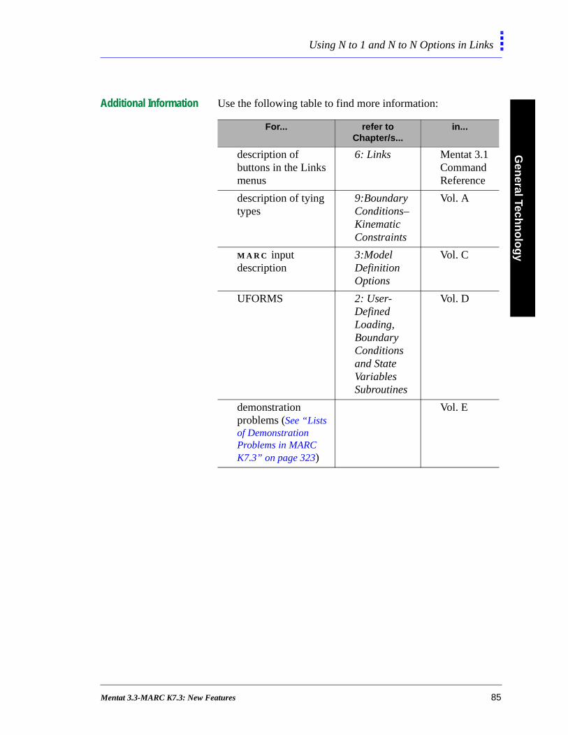
Additional Information Use the following table to find more information:
For... refer to Chapter/s...
in...
description of buttons in the Links menus
6: Links Mentat 3.1 Command Reference
description of tying types
9:Boundary Conditions–Kinematic Constraints
Vol. A
M A R C input description
3:Model Definition Options
Vol. C
UFORMS 2: User-Defined Loading, Boundary Conditions and State Variables Subroutines
Vol. D
demonstration problems (See “Lists of Demonstration Problems in MARC K7.3” on page 323)
Vol. E
Mentat 3.3-MARC K7.3: New Features 85
Gen
eral
Tec
hn
olo
gy
Specifying Node Lists and Node Paths
e
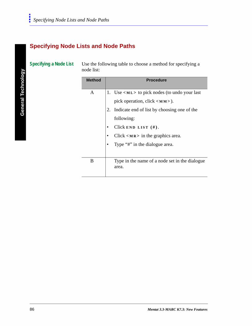
Specifying Node Lists and Node Paths
Specifying a Node List Use the following table to choose a method for specifying a node list:
Method Procedure
A 1. Use < M L > to pick nodes (to undo your last
pick operation, click < M M > ).
2. Indicate end of list by choosing one of the
following:
• Click E N D L I S T ( # ) .
• Click < M R > in the graphics area.
• Type “#” in the dialogue area.
B Type in the name of a node set in the dialoguarea.
86 Mentat 3.3-MARC K7.3: New Features
Gen
eral Techn
olo
gy
Specifying Node Lists and Node Paths
y
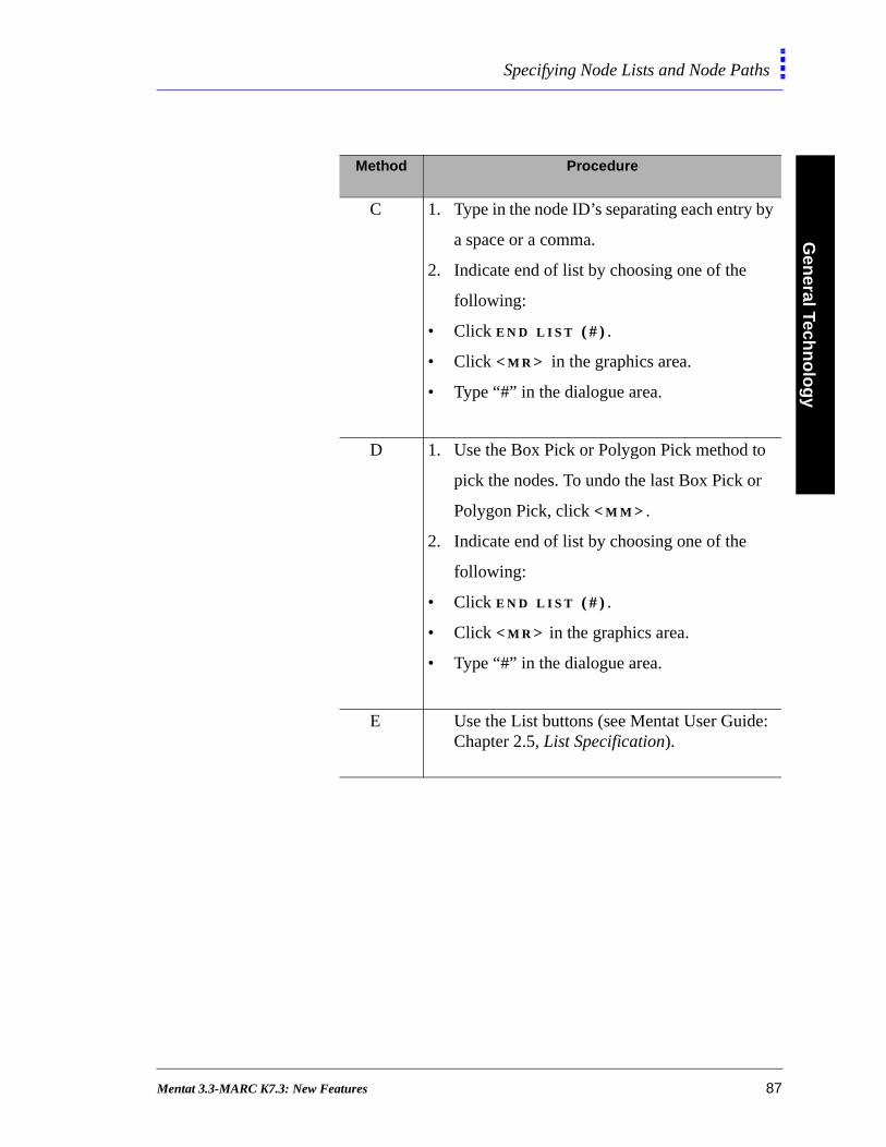
:
C 1. Type in the node ID’s separating each entry b
a space or a comma.
2. Indicate end of list by choosing one of the
following:
• Click E N D L I S T ( # ) .
• Click < M R > in the graphics area.
• Type “#” in the dialogue area.
D 1. Use the Box Pick or Polygon Pick method to
pick the nodes. To undo the last Box Pick or
Polygon Pick, click < M M > .
2. Indicate end of list by choosing one of the
following:
• Click E N D L I S T ( # ) .
• Click < M R > in the graphics area.
• Type “#” in the dialogue area.
E Use the List buttons (see Mentat User GuideChapter 2.5, List Specification).
Method Procedure
Mentat 3.3-MARC K7.3: New Features 87
Gen
eral
Tec
hn
olo
gy
Specifying Node Lists and Node Paths
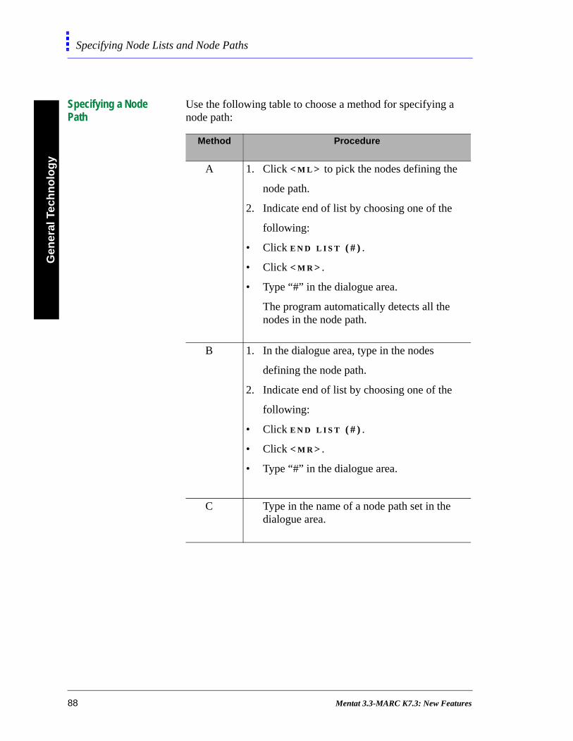
Specifying a Node Path
Use the following table to choose a method for specifying a node path:
Method Procedure
A 1. Click < M L > to pick the nodes defining the
node path.
2. Indicate end of list by choosing one of the
following:
• Click E N D L I S T ( # ) .
• Click < M R > .
• Type “#” in the dialogue area.
The program automatically detects all the nodes in the node path.
B 1. In the dialogue area, type in the nodes
defining the node path.
2. Indicate end of list by choosing one of the
following:
• Click E N D L I S T ( # ) .
• Click < M R > .
• Type “#” in the dialogue area.
C Type in the name of a node path set in the dialogue area.
88 Mentat 3.3-MARC K7.3: New Features
Gen
eral Techn
olo
gy
Specifying Node Lists and Node Paths
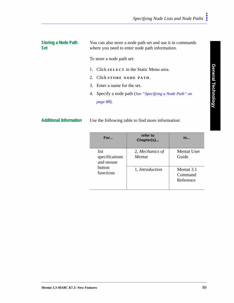
Storing a Node Path Set
You can also store a node path set and use it in commands where you need to enter node path information.
To store a node path set:
1. Click S E L E C T in the Static Menu area.
2. Click S T O R E N O D E P A T H .
3. Enter a name for the set.
4. Specify a node path (See “Specifying a Node Path” on
page 88).
Additional Information Use the following table to find more information:
For...refer to
Chapter(s)...in...
list specifications and mouse button functions
2, Mechanics of Mentat
Mentat User Guide
1, Introduction Mentat 3.1 Command Reference
Mentat 3.3-MARC K7.3: New Features 89

Gen
eral
Tec
hn
olo
gy
Buckle Solutions Using Lanczos Method
he nd
Buckle Solutions Using Lanczos Method
About Lanczos Method for Buckle Solution
You can now use the Lanczos method for buckle eigenvalue extraction analysis in M A R C . There are now two methods for specifying the buckle parameters:
• Lanczos
• Inverse Power Sweep
The Lanczos method is more computationally efficient than tInverse Power Sweep method for relatively larger problems asmall problems that require more than five buckle modes.
Specifying a Buckle Solution Method
To specify a buckle solution method for your job:
1. Choose Jobs>Mechanical>Analysis Options.
2. In the Buckle Solution Method menu area, choose either
L A N C Z O S or I N V E R S E P O W E R S W E E P .
choose abuckle so lu t ionmethod
Jobs>Mechanica l>Analys is Opt ions
90 Mentat 3.3-MARC K7.3: New Features
Gen
eral Techn
olo
gy
Buckle Solutions Using Lanczos Method
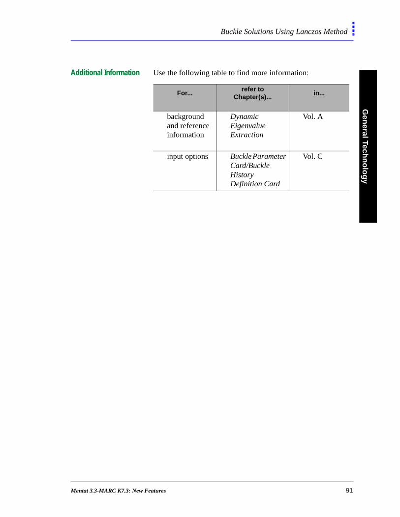
Additional Information Use the following table to find more information:
For...refer to
Chapter(s)...in...
background and reference information
Dynamic Eigenvalue Extraction
Vol. A
input options Buckle Parameter Card/Buckle History Definition Card
Vol. C
Mentat 3.3-MARC K7.3: New Features 91
Gen
eral
Tec
hn
olo
gy
Adaptive Load Stepping
ch
s in
ture
Adaptive Load Stepping
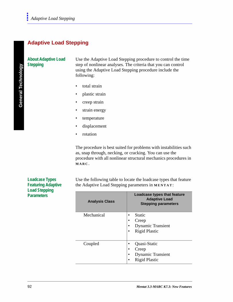
About Adaptive Load Stepping
Use the Adaptive Load Stepping procedure to control the time step of nonlinear analyses. The criteria that you can control using the Adaptive Load Stepping procedure include the following:
• total strain
• plastic strain
• creep strain
• strain energy
• temperature
• displacement
• rotation
The procedure is best suited for problems with instabilities suas, snap through, necking, or cracking. You can use the procedure with all nonlinear structural mechanics procedureM A R C .
Loadcase Types Featuring Adaptive Load Stepping Parameters
Use the following table to locate the loadcase types that feathe Adaptive Load Stepping parameters in M E N T A T :
Analysis Class
Loadcase types that feature Adaptive Load
Stepping parameters
Mechanical • Static• Creep• Dynamic Transient• Rigid Plastic
Coupled • Quasi-Static• Creep• Dynamic Transient• Rigid Plastic
92 Mentat 3.3-MARC K7.3: New Features

Gen
eral Techn
olo
gy
Adaptive Load Stepping
Displaying the Adaptive Load Stepping Parameters
To display the Adaptive Load Stepping parameters:
1. Choose L O A D C A S E S in Main Menu.
2. Choose either M E C H A N I C A L or C O U P L E D .
3. Choose a loadcase type (e.g., Creep).
4. Click P A R A M E T E R S in M E C H . L O A D ( M U L T I -
C R I T E R I A ) .
use these f ieldsto set the genera l parametersfor adapt iveload s tepping
Loadcases>(Mechanica l)>(Creep)>Mechanical Load (Mult i -Cri ter ia) Parameters
.
When you click M E C H . L O A D ( M U L T I - C R I T E R I A ) , it generates the AUTO STEP option in M A R C . This option is similar to the mechanical load equilibrium procedure, which in M A R C W A S called AUTO TIME as a method to control time steps, but is more powerful.
Mentat 3.3-MARC K7.3: New Features 93
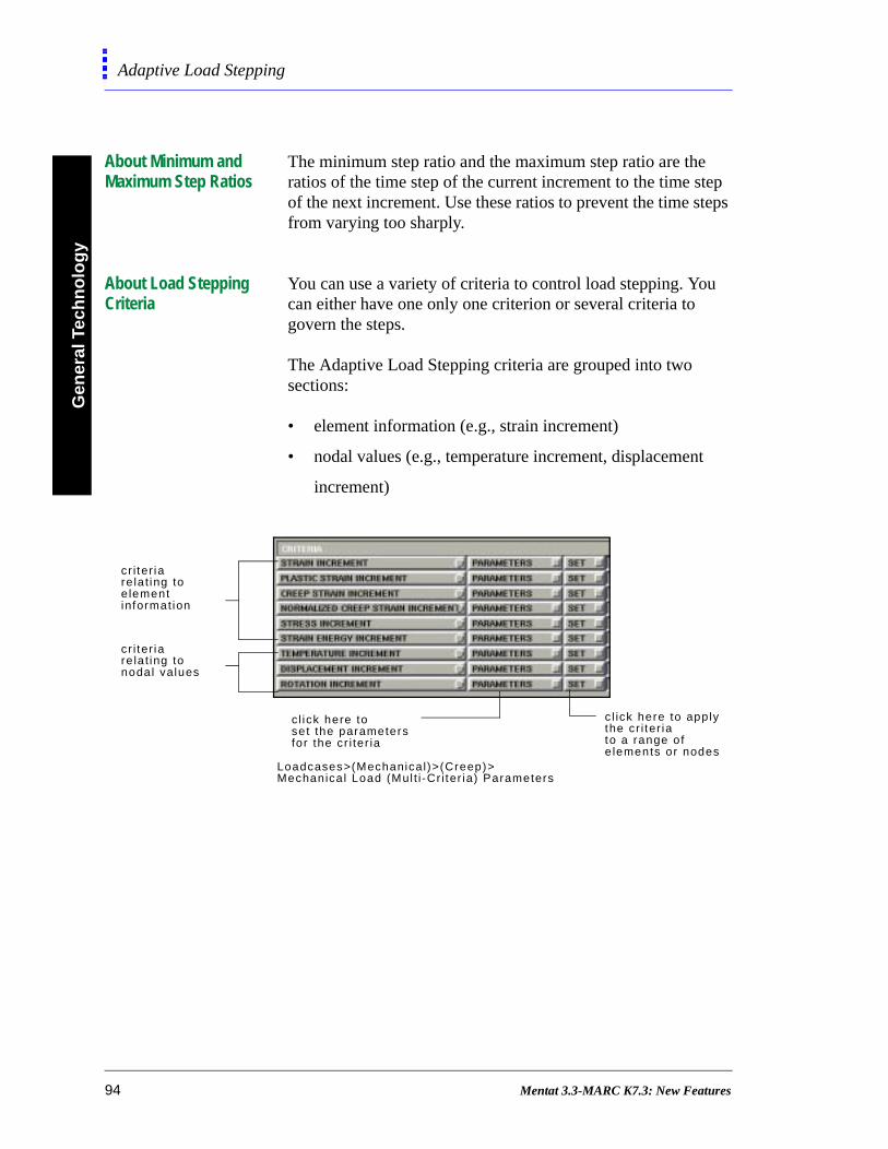
Gen
eral
Tec
hn
olo
gy
Adaptive Load Stepping
About Minimum and Maximum Step Ratios
The minimum step ratio and the maximum step ratio are the ratios of the time step of the current increment to the time step of the next increment. Use these ratios to prevent the time steps from varying too sharply.
About Load Stepping Criteria
You can use a variety of criteria to control load stepping. You can either have one only one criterion or several criteria to govern the steps.
The Adaptive Load Stepping criteria are grouped into two sections:
• element information (e.g., strain increment)
• nodal values (e.g., temperature increment, displacement
increment)
cr i ter iare la t ing toe lementinformat ion
cr i ter ia re la t ing to nodal values
cl ick here toset the parametersfor the cr i ter ia
c l ick here to apply
the cr i ter iato a range of e lements or nodes
Loadcases>(Mechanica l)>(Creep)>Mechanica l Load (Mul t i -Cr i ter ia) Parameters
94 Mentat 3.3-MARC K7.3: New Features

Gen
eral Techn
olo
gy
Adaptive Load Stepping
Setting the Bounds Parameters for a Criterion
To set the bounds for a criterion:
1. Choose L O A D C A S E S in Main Menu.
2. Choose either M E C H A N I C A L or C O U P L E D .
3. Choose a loadcase type (e.g., Creep).
4. Click P A R A M E T E R S in M E C H . L O A D ( M U L T I -
C R I T E R I A ) .
5. Click parameters associated with an increment (e.g., Creep
Strain Increment).
For every criterion that you select, you have to specify a bound on the allowable value of the criterion.
E X A M P L E
If you picked plastic strain increment, you might set a bound to specify that plastic strain increment within a step to be less than, or equal to, 1%. There are two possibilities:
1. If the program performs an increment of analysis and the plastic strain is
greater than 1%, then that increment is recycled with a smaller step.
2. If the increment satisfies the criteria (i.e., strains are less than, or equal
to, 1%), then in the subsequent increments, the time steps increase
because the program can take larger time steps and still satisfy your cri-
teria for accuracy.
Mentat 3.3-MARC K7.3: New Features 95
Gen
eral
Tec
hn
olo
gy
Adaptive Load Stepping
e-
her
r
eep
About Specifying Multiple Ranges for a Criterion
To make adaptive load stepping even more effective, you can specify multiple ranges for a particular criterion.
E X A M P L E
For a plastic strain increment, you can specify the following:
• When the plastic strains are less than 1/10 of 1%, the increments of plas-
tic strain are less than 1/100 of 1%.
• When the plastic strain is less than 2%, you might accept strain incr
ments of 0.1%.
• If the plastic strains are very large (e.g., 10% or 100%), you might
accept strain increments of 1% or 2%.
Applications of Multiple Ranges for Criteria
The criteria that you specify depends on where you are in the analysis or the type of material behavior in the analysis.
Multiple ranges are typically applicable to the following:
• manufacturing problems—where you want to force small
strain increments at the initial yield point of the elastic-
plastic material and you want larger time steps at the hig
range of plastic strain.
• creep analysis—where the material has different behavio
between primary and secondary creep stage or tertiary cr
stage.
96 Mentat 3.3-MARC K7.3: New Features
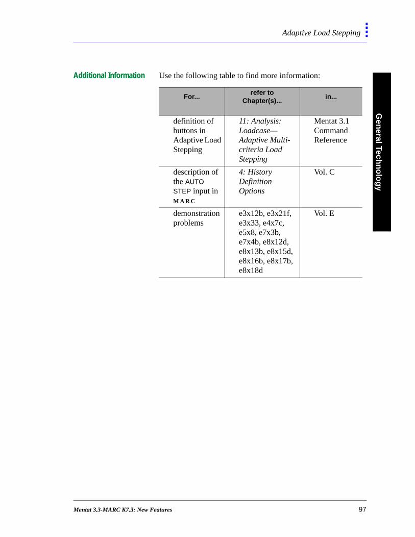
Gen
eral Techn
olo
gy
Adaptive Load Stepping
Additional Information Use the following table to find more information:
For...refer to
Chapter(s)...in...
definition of buttons in Adaptive Load Stepping
11: Analysis: Loadcase—Adaptive Multi-criteria Load Stepping
Mentat 3.1 Command Reference
description of the AUTO STEP input in M A R C
4: History Definition Options
Vol. C
demonstration problems
e3x12b, e3x21f,e3x33, e4x7c,e5x8, e7x3b,e7x4b, e8x12d,e8x13b, e8x15d,e8x16b, e8x17b,e8x18d
Vol. E
Mentat 3.3-MARC K7.3: New Features 97
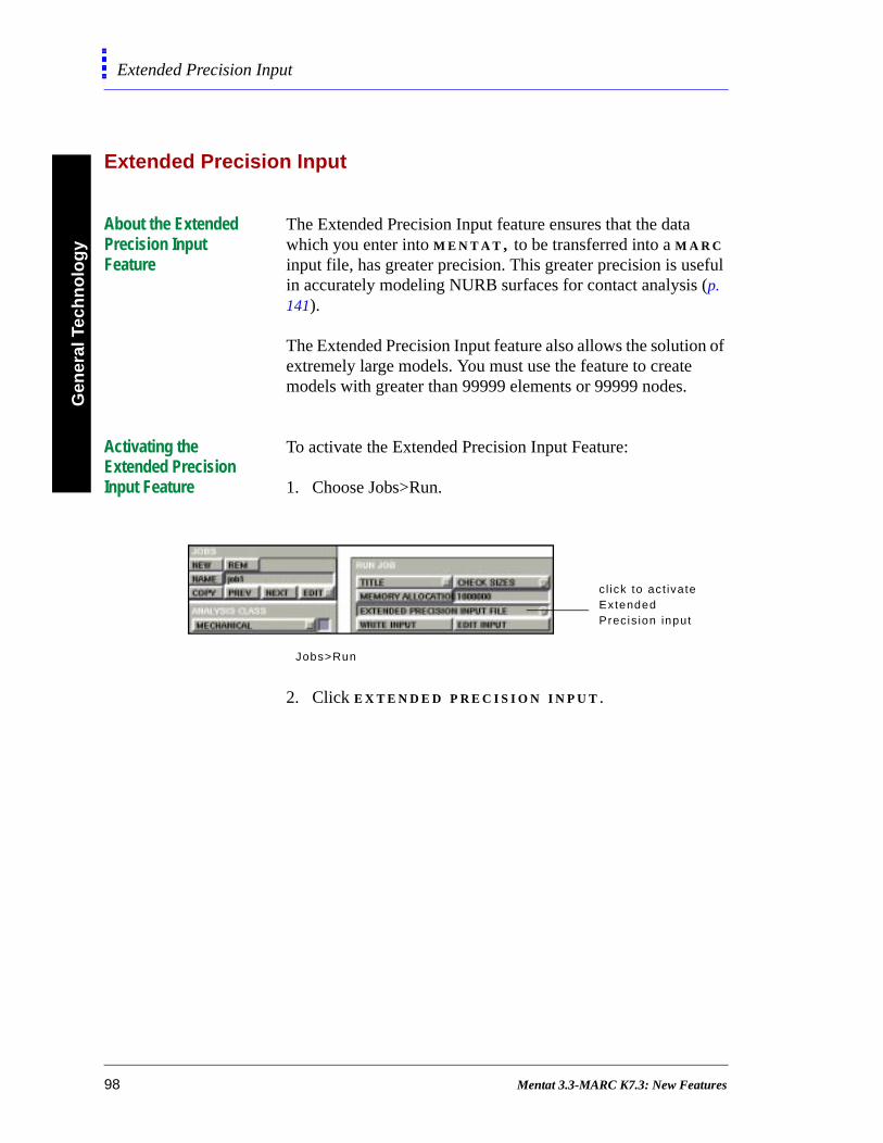
Gen
eral
Tec
hn
olo
gy
Extended Precision Input
Extended Precision Input
About the Extended Precision Input Feature
The Extended Precision Input feature ensures that the data which you enter into M E N T A T , to be transferred into a M A R C input file, has greater precision. This greater precision is useful in accurately modeling NURB surfaces for contact analysis (p. 141).
The Extended Precision Input feature also allows the solution of extremely large models. You must use the feature to create models with greater than 99999 elements or 99999 nodes.
Activating the Extended Precision Input Feature
To activate the Extended Precision Input Feature:
1. Choose Jobs>Run.
2. Click E X T E N D E D P R E C I S I O N I N P U T .
cl ick to act ivateExtended Precis ion input
Jobs>Run
98 Mentat 3.3-MARC K7.3: New Features
Gen
eral Techn
olo
gy
Extended Precision Input
I5
0
Format Changes to Input Files
When you write a M A R C input file using the Extended Precision Input feature, the following format changes occur:
• the EXTENDED parameter is included in the input file.
• all integers are written using the I10 format instead of the
format.
• all floating point numbers are written in the F20 or the F3
format instead of the F10 or the F15 format.
• all character strings are written using the A20 format
instead of the A10 format.
• the input field widths (see Vol. C: Chapter 2–Parameters)
are doubled when you include the EXTENDED parameter.
. You can also mix the formats of an existing inputfile by using the NEW option (see Vol. C: Chapter 4–History Definition Options ).
Mentat 3.3-MARC K7.3: New Features 99
Gen
eral
Tec
hn
olo
gy
Constant Dilatation
Constant Dilatation
When to Use the Constant Dilatation Parameter
Use the Constant Dilatation parameter with element types, 7, 10, 11, 19, or 20, to improve the behavior of these elements for modeling nearly incompressible materials. During elastic-plastic or creep analysis, use the Constant Dilatation parameter for these elements.
However, when you use the multiplicative decomposition, elastic-plastic formulation or the large-strain elasticity formulation in the Updated Lagrange framework, you do not require the Constant Dilatation parameter.
Analysis Classes Featuring the Constant Dilatation Parameter
You can activate the Constant Dilatation parameter for the following analysis classes in M E N T A T :
• Mechanical
• Rigid Plastic
• Coupled
• Coupled Rigid Plastic
100 Mentat 3.3-MARC K7.3: New Features
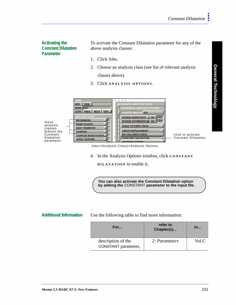
Gen
eral Techn
olo
gy
Constant Dilatation
Activating the Constant Dilatation Parameter
To activate the Constant Dilatation parameter for any of the above analysis classes:
1. Click Jobs.
2. Choose an analysis class (see list of relevant analysis
classes above).
3. Click A N A L Y S I S O P T I O N S .
4. In the Analysis Options window, click C O N S T A N T
D I L A T A T I O N to enable it.
Additional Information Use the following table to find more information:
cl ick to act ivateConstant Di latat ion
Jobs>(Analys is Class)>Analys is Opt ions
theseanalys isc lassesfeature theConstantDi latat ionparameter
. You can also activate the Constant Dilatation option by adding the CONSTANT parameter to the input file.
For...refer to
Chapter(s)...in...
description of the CONSTANT parameter,
2: Parameters Vol.C
Mentat 3.3-MARC K7.3: New Features 101
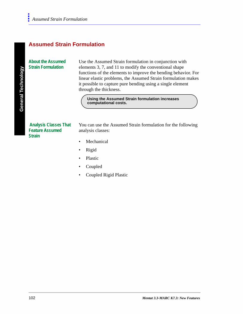
Gen
eral
Tec
hn
olo
gy
Assumed Strain Formulation
Assumed Strain Formulation
About the Assumed Strain Formulation
Use the Assumed Strain formulation in conjunction with elements 3, 7, and 11 to modify the conventional shape functions of the elements to improve the bending behavior. For linear elastic problems, the Assumed Strain formulation makes it possible to capture pure bending using a single element through the thickness.
Analysis Classes That Feature Assumed Strain
You can use the Assumed Strain formulation for the following analysis classes:
• Mechanical
• Rigid
• Plastic
• Coupled
• Coupled Rigid Plastic
. Using the Assumed Strain formulation increasescomputational costs.
102 Mentat 3.3-MARC K7.3: New Features
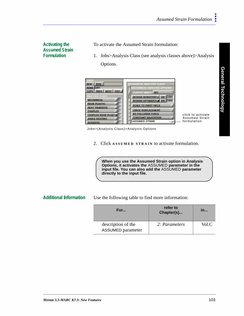
Gen
eral Techn
olo
gy
Assumed Strain Formulation
Activating the Assumed Strain Formulation
To activate the Assumed Strain formulation:
1. Jobs>Analysis Class (see analysis classes above)>Analysis
Options.
2. Click A S S U M E D S T R A I N to activate formulation.
Additional Information Use the following table to find more information:
cl ick to act ivateAssumed Strainformulat ion
Jobs>(Analys is Class)>Analys is Opt ions
.
When you use the Assumed Strain option in Analysis Options, it activates the ASSUMED parameter in theinput file. You can also add the ASSUMED parameterdirectly to the input file.
For...refer to
Chapter(s)...in...
description of the ASSUMED parameter
2: Parameters Vol.C
Mentat 3.3-MARC K7.3: New Features 103

Gen
eral
Tec
hn
olo
gy
Numerical Preferences
Numerical Preferences
About the Numerical Preferences Option
Use the Numerical Preferences option to change the default parameters that control the solution of a numerical analysis. You can use this option for the following analysis classes:
• Mechanical
• Rigid Plastic
• Coupled
• Coupled Rigid Plastic
• Fluid
• Fluid-Thermal
• Fluid-Solid
• Fluid-Thermal-Solid
. The Numerical Preferences option activates the PARAMETERS model definition or history definitionoption.
104 Mentat 3.3-MARC K7.3: New Features
Gen
eral Techn
olo
gy
Numerical Preferences
Activating the Numerical Preferences Option
To activate the Numerical Preferences option:
1. Click J O B S .
2. Choose an analysis class (see valid analysis classes above).
3. Choose Job Parameters>Numerical Preferences.
Additional Information Use the following table to find more information:
opt ions areavai lable or grayed outbased on theanalys is c lass
Jobs>(Analys is Class)>Analys is Opt ions>Job Parameters>Numer ica l Preferences
For...refer to
Chapter(s)...in...
description of the PARAMETER model definition option
3: Model Definition Options
Vol.C
Mentat 3.3-MARC K7.3: New Features 105

Gen
eral
Tec
hn
olo
gy
User-Defined Post Variables
dal
User-Defined Post Variables
About User Subroutine to Write to the Post File
There are three user subroutines to define the quantities to write to the post file during an analysis:
• ELEVAR—output of element quantities
• ELEVEC—output of element quantities in harmonic
analysis
• UPOSTV—(new user subroutine) user-selected post-
processing of nodal variables
The new user subroutine, UPOSTV, enables you to define novectors.
Activating the User Subroutine UPOSTV
To activate the user subroutine UPOSTV:
1. Click Jobs>(Analysis Class)>Job Results.
enter numberof vectors
Jobs>(Analys is Class)>Job Resul ts
106 Mentat 3.3-MARC K7.3: New Features
Gen
eral Techn
olo
gy
User-Defined Post Variables
2. Click # U S E R D E F I N E D N O D A L V E C T O R S and enter
the number of vectors.
Additional Information Use the following table to find more information:
.
As an alternative, you can modify the POST modeldefinition option (See Vol. C: Chap.3–Program Control ).It is also necessary to write the user subroutine and include it with any other user subroutines.
For...refer to
Chapter(s)...in...
description of the user subroutine, UPOSTV
7: Output Quantities
Vol.D
Mentat 3.3-MARC K7.3: New Features 107

Mentat 3.3-MARC K7.3: New Features
5• Mesh Generation
Repair Geometry
Trimming Surfaces 114About Tolerance Value for Curve Intersection 120
Curve Divisions
Applying Fixed Divisions to a Curve 123Parameters for Curvature-Dependent Curve Divisions 124
Using the Advancing Front Mesher
Special Considerations for Quad Meshing 129Specifying Distortion Parameters 131
Using the Delaunay Mesher
Features of the Delaunay mesher 133Applying the Delaunay Mesher 134
Expanding Elements Along a Curve
About Expanding Elements Along a Curve in Mentat 3.3 135
Creating a Node Point at Midpoint
Mentat 3.3-MARC K7.3: New Features 109

Creating a New Point 138
Mentat 3.3-MARC K7.3: New Features

Mesh
Gen
eration
Mentat 3.3-MARC K7.3: New Features 111

Mes
h G
ener
atio
n
• Mesh Generation
112 Mentat 3.3-MARC K7.3: New Features

Mesh
Gen
eration
Repair Geometry
Repair Geometry
About Repair Geometry Operations
Use the Repair Geometry menus to clean up the geometric data for curves and surfaces when you import a CAD geometry.
use the Repai rGeometry commandsfor e i ther curvesor sur faces
Mesh Generat ion>Automesh>Repair Geometry
. The Repair Geometry operations change your model.
Save the current model before you use the RepairGeometry commands.
Mentat 3.3-MARC K7.3: New Features 113

Mes
h G
ener
atio
nRepair Geometry
Adding/Removing Geometry
Trimming Surfaces Very often, when you import geometries into M E N T A T , some or all of the trimming curves for some surfaces are missing. Use the Trim Surface command to place four trimming curves on the edges of surfaces.
To trim surfaces:
1. Choose Mesh Generation>Automesh>Repair Geometry.
2. Click T R I M S U R F A C E S .
3. Enter a surface list.
Removing Free Curves To remove curves not attached to any surface, choose Mesh Generation>Automesh>Repair Geometry> Remove Free Curves.
Mesh Generat ion>Repai r Geometry>Remove Free Curves
114 Mentat 3.3-MARC K7.3: New Features
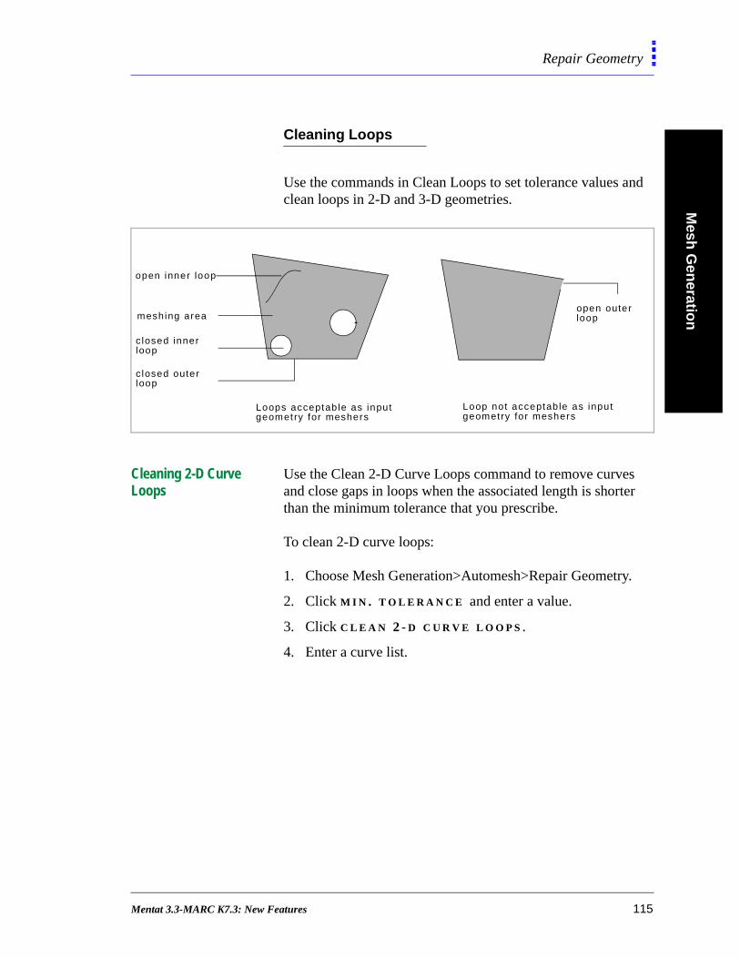
Mesh
Gen
eration
Repair Geometry
Cleaning Loops
Use the commands in Clean Loops to set tolerance values and clean loops in 2-D and 3-D geometries.
Cleaning 2-D Curve Loops
Use the Clean 2-D Curve Loops command to remove curves and close gaps in loops when the associated length is shorter than the minimum tolerance that you prescribe.
To clean 2-D curve loops:
1. Choose Mesh Generation>Automesh>Repair Geometry.
2. Click M I N . T O L E R A N C E and enter a value.
3. Click C L E A N 2 - D C U R V E L O O P S .
4. Enter a curve list.
c losed inner
meshing area
open inner loop
c losed outer
loop
loop
Loops acceptable as inputgeometry for meshers
open outerloop
Loop not acceptable as inputgeometry for meshers
Mentat 3.3-MARC K7.3: New Features 115
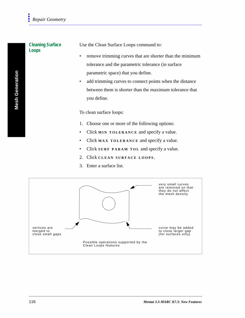
Mes
h G
ener
atio
nRepair Geometry
m
t
Cleaning Surface Loops
Use the Clean Surface Loops command to:
• remove trimming curves that are shorter than the minimu
tolerance and the parametric tolerance (in surface
parametric space) that you define.
• add trimming curves to connect points when the distance
between them is shorter than the maximum tolerance tha
you define.
To clean surface loops:
1. Choose one or more of the following options:
• Click M I N T O L E R A N C E and specify a value.
• Click M A X T O L E R A N C E and specify a value.
• Click S U R F P A R A M T O L and specify a value.
2. Click C L E A N S U R F A C E L O O P S .
3. Enter a surface list.
very smal l curvesare removed so that
curve may be addedto c lose larger gap( for sur faces only)
ver t ices aremerged to c lose smal l gaps
Possib le operat ions suppor ted by theClean Loops features
they do not a ffectthe mesh density
116 Mentat 3.3-MARC K7.3: New Features
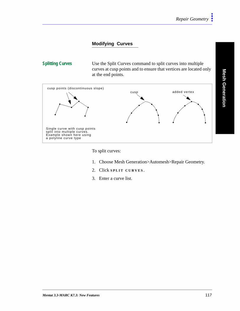
Mesh
Gen
eration
Repair Geometry
Modifying Curves
Splitting Curves Use the Split Curves command to split curves into multiple curves at cusp points and to ensure that vertices are located only at the end points.
To split curves:
1. Choose Mesh Generation>Automesh>Repair Geometry.
2. Click S P L I T C U R V E S .
3. Enter a curve list.
cusp points (d iscont inuous s lope)
Single curve wi th cusp points
Example shown here us ingspl i t in to mult ip le curves.
a po ly l ine curve type
cusp added ver tex
Mentat 3.3-MARC K7.3: New Features 117

Mes
h G
ener
atio
nRepair Geometry
Breaking Curves There are cases where two trimming surfaces may share a common geometric curve but have different trimming curves. To make all trimming curves compatible, use the Break Curves command.
To break a curve:
1. Choose Mesh Generation>Automesh>Repair Geometry.
2. Click B R E A K C U R V E S .
3. Enter a vertex tolerance.
4. Enter a curve list.
Pi1 P j1
Pj2
Pj3Pi2
sur face i
surface j
P i1
Pi2
Pi3
Pj1
Pj2
Pj3
surface i
sur facej
Before Break Operat ion After Break Operat ion
tr immingcurves P i1Pi2,Pj1Pj2, Pj2Pj3 arenot compat ible
curvesare compat ib le
curvesare compat ible
118 Mentat 3.3-MARC K7.3: New Features
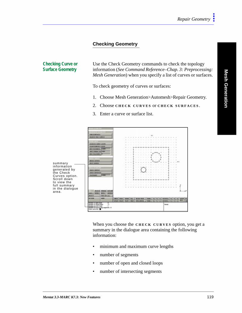
Mesh
Gen
eration
Repair Geometry
ng:
Checking Geometry
Checking Curve or Surface Geometry
Use the Check Geometry commands to check the topology information (See Command Reference–Chap. 3: PreprocessiMesh Generation) when you specify a list of curves or surfaces.
To check geometry of curves or surfaces:
1. Choose Mesh Generation>Automesh>Repair Geometry.
2. Choose C H E C K C U R V E S or C H E C K S U R F A C E S .
3. Enter a curve or surface list.
When you choose the C H E C K C U R V E S option, you get a summary in the dialogue area containing the following information:
• minimum and maximum curve lengths
• number of segments
• number of open and closed loops
• number of intersecting segments
summaryin format iongenerated bythe CheckCurves opt ion.Scro l l downto v iew thefu l l summaryin the d ia loguearea.
Mentat 3.3-MARC K7.3: New Features 119
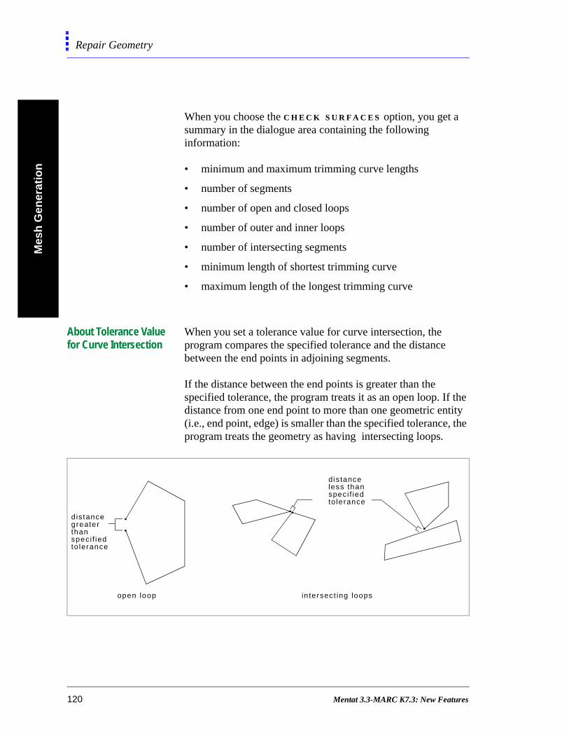
Mes
h G
ener
atio
nRepair Geometry
the ity the
When you choose the C H E C K S U R F A C E S option, you get a summary in the dialogue area containing the following information:
• minimum and maximum trimming curve lengths
• number of segments
• number of open and closed loops
• number of outer and inner loops
• number of intersecting segments
• minimum length of shortest trimming curve
• maximum length of the longest trimming curve
About Tolerance Value for Curve Intersection
When you set a tolerance value for curve intersection, the program compares the specified tolerance and the distancebetween the end points in adjoining segments.
If the distance between the end points is greater than the specified tolerance, the program treats it as an open loop. Ifdistance from one end point to more than one geometric ent(i.e., end point, edge) is smaller than the specified tolerance,program treats the geometry as having intersecting loops.
open loop intersect ing loops
dis tancegreaterthanspecif iedto lerance
distanceless thanspeci f iedto lerance
120 Mentat 3.3-MARC K7.3: New Features
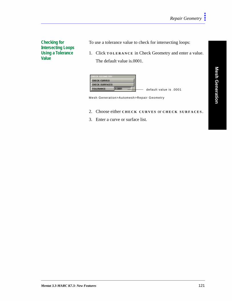
Mesh
Gen
eration
Repair Geometry
Checking for Intersecting Loops Using a Tolerance Value
To use a tolerance value to check for intersecting loops:
1. Click T O L E R A N C E in Check Geometry and enter a value.
The default value is.0001.
2. Choose either C H E C K C U R V E S or C H E C K S U R F A C E S .
3. Enter a curve or surface list.
Mesh Generat ion>Automesh>Repair Geometry
defaul t va lue is .0001
Mentat 3.3-MARC K7.3: New Features 121

Mes
h G
ener
atio
nCurve Divisions
et
in
Curve Divisions
About Curve Divisions You can specify three types of curve divisions in M E N T A T :
• fixed number of divisions—the number of divisions along
the curve is fixed by the number of divisions that you
specify. All segments along the curve have equal length.
• fixed average length—each segment along the curve is s
as close as possible to the value that you define as the
average length.
• curvature dependent—the length of each segment varies
with the curvature along the curve according to the
parameters that you specify. All segment lengths are with
the range prescribed in the M I N L E N G T H and M A X
L E N G T H fields.
defaul t set t ing isFIXED # DIVISIONS
Mesh Generat ion>Automesh>Curve Div is ions
. You can choose only one type of curve division
at a time.
122 Mentat 3.3-MARC K7.3: New Features
Mesh
Gen
eration
Curve Divisions
Applying Fixed Divisions to a Curve
To apply a fixed division to curves:
1. Choose Mesh Generation>Automesh>Curve Divisions.
2. Click F I X E D # D I V I S I O N S .
3. Click # D I V I S I O N S and enter a value.
4. Click A P P L Y C U R V E D I V I S I O N s.
5. Enter a curve list.
Applying Fixed Average Length Divisions
To apply a fixed average length to a curve:
1. Choose Mesh Generation>Automesh>Curve Divisions.
2. Click F I X E D A V G . L E N G T H .
3. Click A V G . L E N G T H and enter a value.
4. Click A P P L Y C U R V E D I V I S I O N S .
5. Enter a curve list.
About Curvature-Dependent Curve Divisions
Use curvature-dependent curve divisions to produce curve divisions that are consistent with curve shape.
Here are some benefits of using curvature-dependent divisions:
• minimum number of divisions generated over straight
portions of the curve
• more division edges generated over the high curvature
portion of the curve
Mentat 3.3-MARC K7.3: New Features 123

Mes
h G
ener
atio
nCurve Divisions
lute
ing
Parameters for Curvature-Dependent Curve Divisions
To apply curvature-dependent divisions to a curve, specify the following parameters:
• M I N . L E N G T H : the minimum length of segments
generated by the curve division operation.
• M A X . L E N G T H : the maximum length of segments
generated by the curve division operation.
• T O L E R A N C E : the maximum allowable deviation of
straight division segments to the curve, given as an abso
distance value (A B S ) , or a value which is relative to the
edge segment length (R E L ).
Applying Curvature-Dependent Divisions to a Curve
To apply curvature-dependent curve divisions to a curve:
1. Choose Mesh Generation>Automesh>Curve Divisions.
2. Click C U R V A T U R E D E P E N D E N T .
3. Click M I N L E N G T H and enter a value.
4. Click M A X L E N G T H and enter a value.
5. Click T O L E R A N C E and enter a value.
6. Choose R E L or A B S in the tolerance option (the default
value is R E L ).
7. Click A P P L Y C U R V E D I V I S I O N S .
8. Enter a curve list.
The tolerance options mentioned above work in the same manner as the tolerance options described in Adaptive Plott(See “Tolerance and Modes of Tolerances” on page 52).
124 Mentat 3.3-MARC K7.3: New Features

Mesh
Gen
eration
Curve Divisions
Applying Restrictions to Individual Curves and Detected Loops
Use the Restriction menus to force even or odd divisions on individual curves or detected loops (See Mentat 3.1 Command Reference–Chapter 3, Preprocessing: Mesh Generation).
1. Choose Mesh Generation>Automesh>Curve Divisions.
2. In the Apply Restriction To area, choose individual curves
or detected loops.
3. Choose F O R C E E V E N D I V or F O R C E O D D D I V.
4. Click A P P L Y C U R V E D I V I S I O N S .
5. Enter a curve list.
You can specify a fixed number of divisions, N, for curve divisions. If the number, N, conflicts with the restriction type, the resulting division has one more division than the value of N.
.
When you apply the even/odd restriction on detected loops within the given curves, the restriction is only enforcedon entire closed loops and individual curves may notnecessarily meet the criteria. This might cause problemswhen you try to match divisions for corresponding curveson surfaces.
Mentat 3.3-MARC K7.3: New Features 125

Mes
h G
ener
atio
nCurve Divisions
Matching Curves Use the Match Curves command to ensure that the number of mesh divisions of coincident curves is equal. The curves are matched based on a vertex tolerance that you specify.
To match curves:
1. Choose Mesh Generation>Automesh>Curve Divisions.
2. Click M A T C H C U R V E D I V I S I O N S .
3. Enter a value for the vertex tolerance.
4. Enter a curve list.
When to Break or Match Curves
Use the table to determine when to break (See “Breaking Curves” on page 118) or match curves:
before matching curves after matching curves
.
The Match Curves command changes the divisions on certain curves where necessary and might disrupt theodd/even restrictions that you had applied when you created the curve divisions.
If...then, use this
operation:
neighboring trimming curves are not coincident over their entire lengths
Break
you applied curve divisions and there are coincident neighboring curves with non-conforming divisions
Match
126 Mentat 3.3-MARC K7.3: New Features
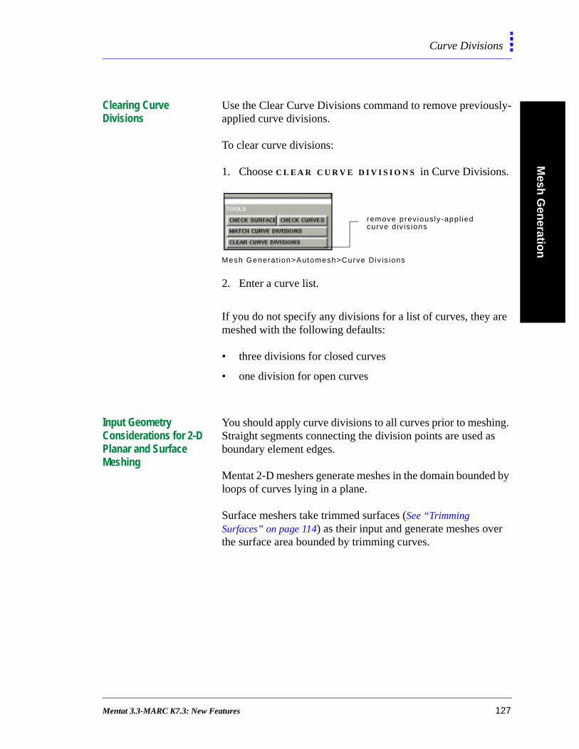
Mesh
Gen
eration
Curve Divisions
g. s
d by
Clearing Curve Divisions
Use the Clear Curve Divisions command to remove previously-applied curve divisions.
To clear curve divisions:
1. Choose C L E A R C U R V E D I V I S I O N S in Curve Divisions.
2. Enter a curve list.
If you do not specify any divisions for a list of curves, they are meshed with the following defaults:
• three divisions for closed curves
• one division for open curves
Input Geometry Considerations for 2-D Planar and Surface Meshing
You should apply curve divisions to all curves prior to meshinStraight segments connecting the division points are used aboundary element edges.
Mentat 2-D meshers generate meshes in the domain boundeloops of curves lying in a plane.
Surface meshers take trimmed surfaces (See “Trimming Surfaces” on page 114) as their input and generate meshes over the surface area bounded by trimming curves.
Mesh Generat ion>Automesh>Curve Div is ions
remove previously-appl iedcurve d iv is ions
Mentat 3.3-MARC K7.3: New Features 127

Mes
h G
ener
atio
nCurve Divisions
s
ke
Guidelines for Using 2-D and Surface Meshers
For 2-D meshers, you should enter a list of coplanar curves. The mesh area lies within closed loops formed by the curves.
For surfaces meshers, you should enter a list of surfaces. The mesh area on each surface lies between closed loops formed by trimming curves attached to that surface.
Guidelines for Inner and Outer Loops
You can use the 2-D and surface meshers for models that contain:
• closed inner and outer loops
• open inner loops
When you use both inner and outer loops, the mesh area liebetween them.
Checklist for the Advancing Front and Delaunay Meshers
Before using the 2-D or surface meshers on your model, masure that:
• there is at least one outer loop
• all open loops are contained within a closed loop
• all the curves have divisions applied to them
• no loops intersect
.
Do not use 2-D planar meshers to generate meshes over planar surfaces in analyses that are not 2-D. Otherwise, the resulting mesh will not be attachedto the surface and will not adhere to any boundaryconditions for that surface.
128 Mentat 3.3-MARC K7.3: New Features
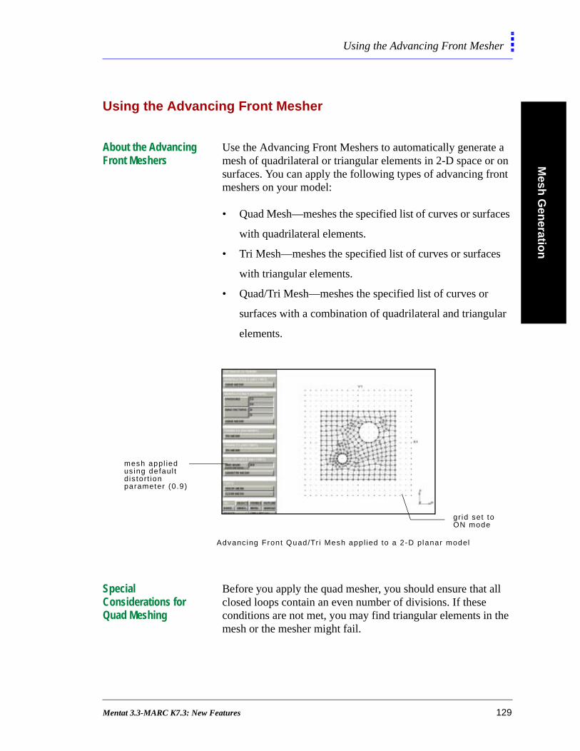
Mesh
Gen
eration
Using the Advancing Front Mesher
ces
s
r
ll
he
Using the Advancing Front Mesher
About the Advancing Front Meshers
Use the Advancing Front Meshers to automatically generate a mesh of quadrilateral or triangular elements in 2-D space or on surfaces. You can apply the following types of advancing front meshers on your model:
• Quad Mesh—meshes the specified list of curves or surfa
with quadrilateral elements.
• Tri Mesh—meshes the specified list of curves or surface
with triangular elements.
• Quad/Tri Mesh—meshes the specified list of curves or
surfaces with a combination of quadrilateral and triangula
elements.
Special Considerations for Quad Meshing
Before you apply the quad mesher, you should ensure that aclosed loops contain an even number of divisions. If these conditions are not met, you may find triangular elements in tmesh or the mesher might fail.
Advancing Front Quad/Tr i Mesh appl ied to a 2-D planar model
gr id set toON mode
mesh appl iedusing defaul tdis tort ionparameter (0.9)
Mentat 3.3-MARC K7.3: New Features 129
Mes
h G
ener
atio
nUsing the Advancing Front Mesher
About Distortion Parameters in Quad/Tri Meshing
When you use the Quad/Tri Mesher, you should specify the maximum allowable distortion of the quadrilateral elements in the mesh using the Max. Quad. Distortion parameter. A distortion parameter is a measure of how closely an element resembles its parent element which, for a quad element, is a rectangle. The value of a distortion parameter may range from 0.0 (perfect rectangle) to 1.0 (collapsed or obtuse).
When you mesh your model with the Quad/Tri mesher, the preferred elements are quadrilateral and no element is allowed to have a distortion parameter greater than the prescribed value of the Max. Quad. Distortion parameter.
If you set the value of the parameter to 1.0 (full quad distortion) and all the closed loops have an even number of boundary divisions, then the resulting mesh is an all-quad mesh. If you set the value to 0.0 (no quad distortion), the resulting mesh is an all-tri mesh.
Considerations for Specifying Distortion Parameters
Although the value of the Max. Quad. Distortion parameter ranges from 0.0 to 1.0, you may want to specify a value that is greater than 0.5. The higher the value of the distortion parameter, the more quads that make up the final mesh. The mesher always tries to place quad elements first.
If you enter a very low value of the distortion parameter (i.e., a value closer to 0.0), it slows down the mesher considerably while generating a predominantly tri-mesh.
You might discover that in most cases, the more practical values for the distortion parameter lie in the 0.9-1.0 range. In that range, the mesh is a predominantly-quad mesh.
130 Mentat 3.3-MARC K7.3: New Features
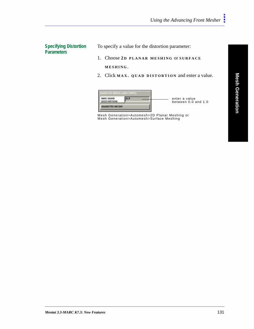
Mesh
Gen
eration
Using the Advancing Front Mesher
Specifying Distortion Parameters
To specify a value for the distortion parameter:
1. Choose 2 D P L A N A R M E S H I N G or S U R F A C E
M E S H I N G .
2. Click M A X . Q U A D D I S T O R T I O N and enter a value.
Mesh Generat ion>Automesh>2D Planar Meshing orMesh Generat ion>Automesh>Surface Meshing
enter a value between 0.0 and 1.0
Mentat 3.3-MARC K7.3: New Features 131
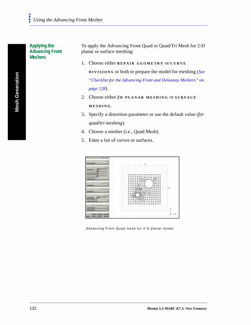
Mes
h G
ener
atio
nUsing the Advancing Front Mesher
Applying the Advancing Front Meshers
To apply the Advancing Front Quad or Quad/Tri Mesh for 2-D planar or surface meshing:
1. Choose either R E P A I R G E O M E T R Y or C U R V E
D I V I S I O N S or both to prepare the model for meshing (See
“Checklist for the Advancing Front and Delaunay Meshers” on
page 128).
2. Choose either 2 D P L A N A R M E S H I N G or S U R F A C E
M E S H I N G .
3. Specify a distortion parameter or use the default value (for
quad/tri meshing).
4. Choose a mesher (i.e., Quad Mesh).
5. Enter a list of curves or surfaces.
Advancing Front Quad mesh for 2-D p lanar model
132 Mentat 3.3-MARC K7.3: New Features
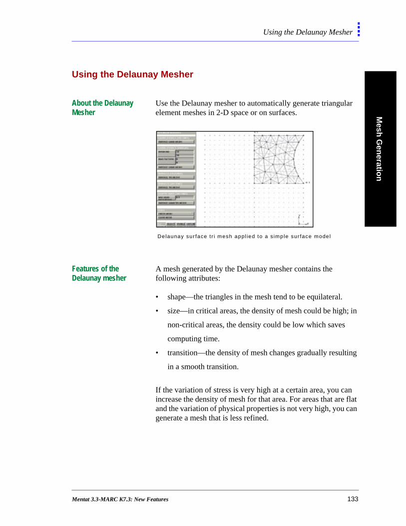
Mesh
Gen
eration
Using the Delaunay Mesher
in
ing
n flat an
Using the Delaunay Mesher
About the Delaunay Mesher
Use the Delaunay mesher to automatically generate triangular element meshes in 2-D space or on surfaces.
Features of the Delaunay mesher
A mesh generated by the Delaunay mesher contains the following attributes:
• shape—the triangles in the mesh tend to be equilateral.
• size—in critical areas, the density of mesh could be high;
non-critical areas, the density could be low which saves
computing time.
• transition—the density of mesh changes gradually result
in a smooth transition.
If the variation of stress is very high at a certain area, you caincrease the density of mesh for that area. For areas that areand the variation of physical properties is not very high, you cgenerate a mesh that is less refined.
Delaunay sur face t r i mesh appl ied to a s imple sur face model
Mentat 3.3-MARC K7.3: New Features 133
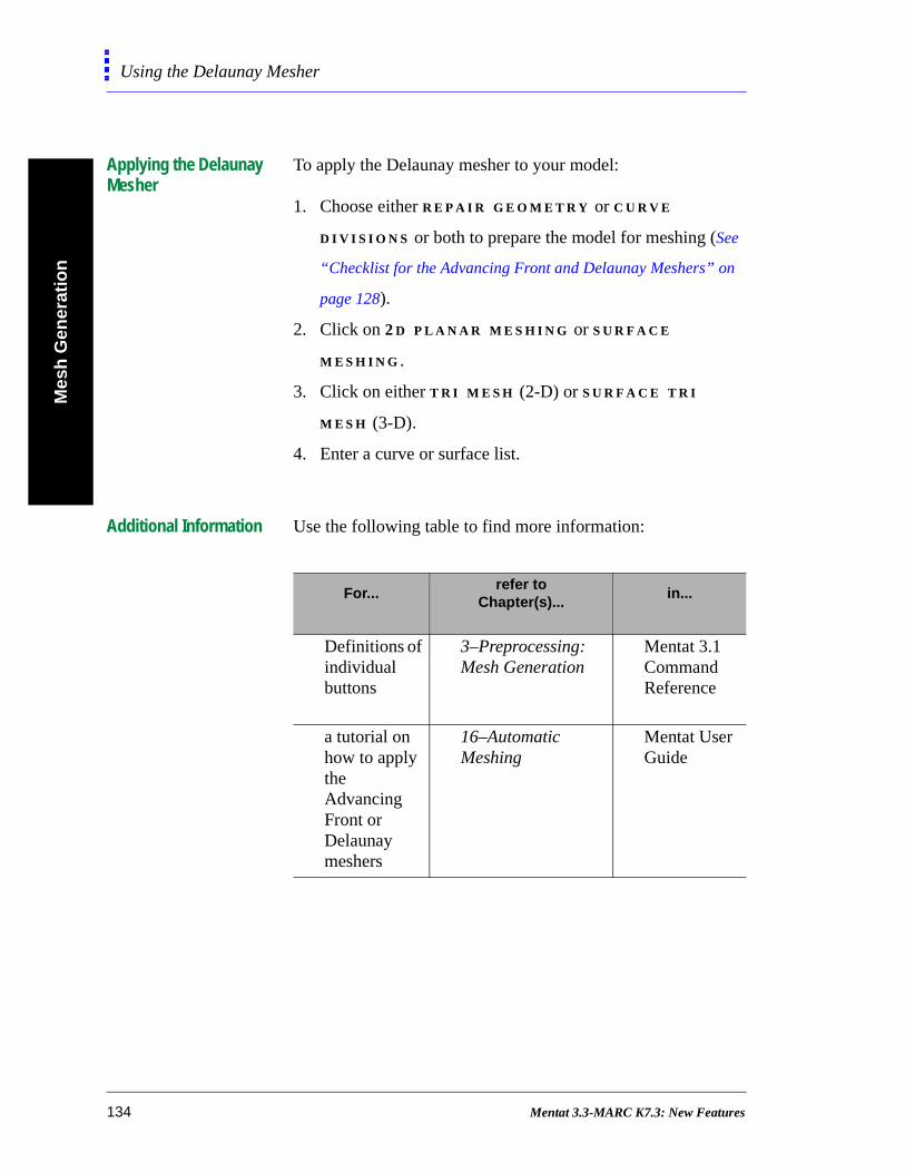
Mes
h G
ener
atio
nUsing the Delaunay Mesher
Applying the Delaunay Mesher
To apply the Delaunay mesher to your model:
1. Choose either R E P A I R G E O M E T R Y or C U R V E
D I V I S I O N S or both to prepare the model for meshing (See
“Checklist for the Advancing Front and Delaunay Meshers” on
page 128).
2. Click on 2 D P L A N A R M E S H I N G or S U R F A C E
M E S H I N G .
3. Click on either T R I M E S H (2-D) or S U R F A C E T R I
M E S H (3-D).
4. Enter a curve or surface list.
Additional Information Use the following table to find more information:
For...refer to
Chapter(s)...in...
Definitions of individual buttons
3–Preprocessing: Mesh Generation
Mentat 3.1 Command Reference
a tutorial on how to apply the Advancing Front or Delaunay meshers
16–Automatic Meshing
Mentat User Guide
134 Mentat 3.3-MARC K7.3: New Features
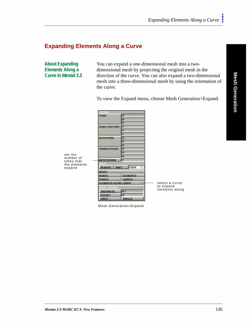
Mesh
Gen
eration
Expanding Elements Along a Curve
Expanding Elements Along a Curve
About Expanding Elements Along a Curve in Mentat 3.3
You can expand a one-dimensional mesh into a two-dimensional mesh by projecting the original mesh in the direction of the curve. You can also expand a two-dimensional mesh into a three-dimensional mesh by using the orientation of the curve.
To view the Expand menu, choose Mesh Generation>Expand.
Mesh Generat ion>Expand
set the number of t imes thatthe e lementsexpand
select a curveto expand e lements along
Mentat 3.3-MARC K7.3: New Features 135
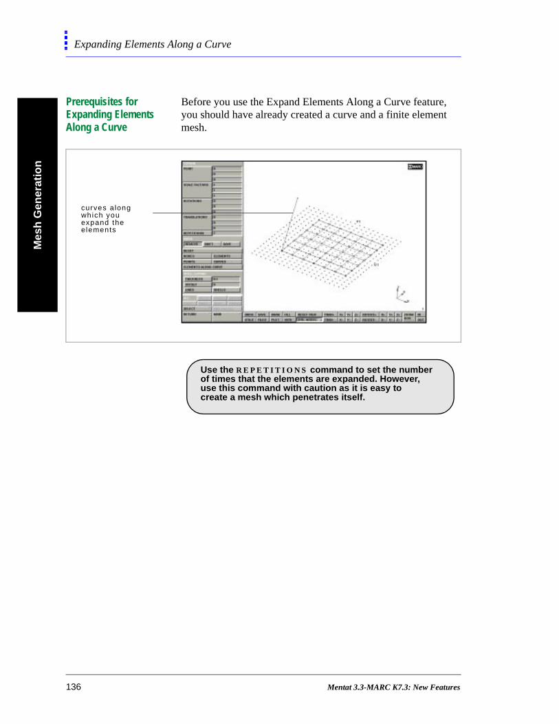
Mes
h G
ener
atio
nExpanding Elements Along a Curve
Prerequisites for Expanding Elements Along a Curve
Before you use the Expand Elements Along a Curve feature, you should have already created a curve and a finite element mesh.
curves a longwhich you expand the elements
.
Use the R E P E T I T I O N S command to set the number of times that the elements are expanded. However,use this command with caution as it is easy to create a mesh which penetrates itself.
136 Mentat 3.3-MARC K7.3: New Features
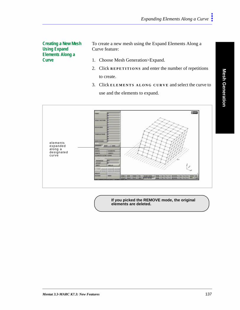
Mesh
Gen
eration
Expanding Elements Along a Curve
Creating a New Mesh Using Expand Elements Along a Curve
To create a new mesh using the Expand Elements Along a Curve feature:
1. Choose Mesh Generation>Expand.
2. Click R E P E T I T I O N S and enter the number of repetitions
to create.
3. Click E L E M E N T S A L O N G C U R V E and select the curve to
use and the elements to expand.
elements expandedalong adesignatedcurve
. If you picked the REMOVE mode, the original
elements are deleted.
Mentat 3.3-MARC K7.3: New Features 137
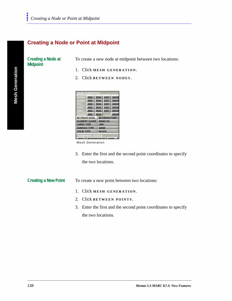
Mes
h G
ener
atio
nCreating a Node or Point at Midpoint
Creating a Node or Point at Midpoint
Creating a Node at Midpoint
To create a new node at midpoint between two locations:
1. Click M E S H G E N E R A T I O N .
2. Click B E T W E E N N O D E S .
3. Enter the first and the second point coordinates to specify
the two locations.
Creating a New Point To create a new point between two locations:
1. Click M E S H G E N E R A T I O N .
2. Click B E T W E E N P O I N T S .
3. Enter the first and the second point coordinates to specify
the two locations.
Mesh Generat ion
138 Mentat 3.3-MARC K7.3: New Features
6• Contact
Performing Contact Analyses
Components of a Contact Analysis 141Choosing a Contact Body Type 143Analysis Parameters for Deformable Bodies 145About Rigid Bodies and Their Representation 148About Velocity as Rigid Body Motion Control 150Coupled Analysis Considerations 152About Contact Tables 154About Exclude Segments 157
Specifying Contact Information in Loadcases
About Contact Information and Loadcases in Analysis 158
Specifying Contact Information in Jobs
About Contact Control in Jobs 161About User Subroutines 162About Increment Splitting 164About Separation Procedures 165About Friction Models 166About Stick-slip 168
Mentat 3.3-MARC K7.3: New Features 139

• Contact
Mentat 3.3-MARC K7.3: New Features
Co
ntact
Performing Contact Analyses
nal
-D
e
e is
he
a
ier
e
Performing Contact Analyses
Components of a Contact Analysis
The contact analysis process has the following components:
• define different contact bodies—bodies can be conventio
deformable bodies made up of finite elements or rigid
bodies made up of either curves for 2-D, or surfaces for 3
analyses (See “Choosing a Contact Body Type” on page 143).
• determine the contact tolerances—establish how close th
body needs to be with another body to conclude that ther
contact between the two bodies (See “About Contact
Tolerances” on page 163).
• define where the contact potentially occurs—by default, t
system assumes that any point on the outside surface of
body can contact any other body. While this makes it eas
to define contact, it might lead to higher computational
costs (See “About Contact Areas” on page 156).
• prescribe different contact procedures in MARC—how th
numerical algorithms are implemented in the analysis (See
“About Contact Control in Jobs” on page 161).
• prescribe separation procedures—how a body separates
from another body (See “About Separation Procedures” on
page 165).
Mentat 3.3-MARC K7.3: New Features 141
Co
nta
ctPerforming Contact Analyses
es
e
ry
• specify the type of friction—which type of friction model to
use; assign the coefficients of friction between the surfac
of the two different bodies (See “About Friction Models” on
page 166).
• assign the parameters for coupled analysis—evaluate th
thermal interactions between two adjacent bodies (See
“Coupled Analysis Considerations” on page 152).
About Physical Bodies When you are defining physical bodies, you can specify one or more of the following conditions:
• one of the bodies is deformable
• multiple bodies are deformable
• one deformable body is in self-contact
• multiple bodies are rigid
About Contact Bodies In M E N T A T , there are four different types of contact bodies:
• Deformable
• Rigid—the body is either moving in space or is a special
type of rigid body.
• Symmetry—special type of rigid body which is a symmet
line or a symmetry surface.
• Rigid with Heat Transfer—a body made up of finite
elements and is not deformable; used only in coupled
thermal stress analysis. This is a region comprising of
. You should define at least one deformable body
in the analysis.
142 Mentat 3.3-MARC K7.3: New Features
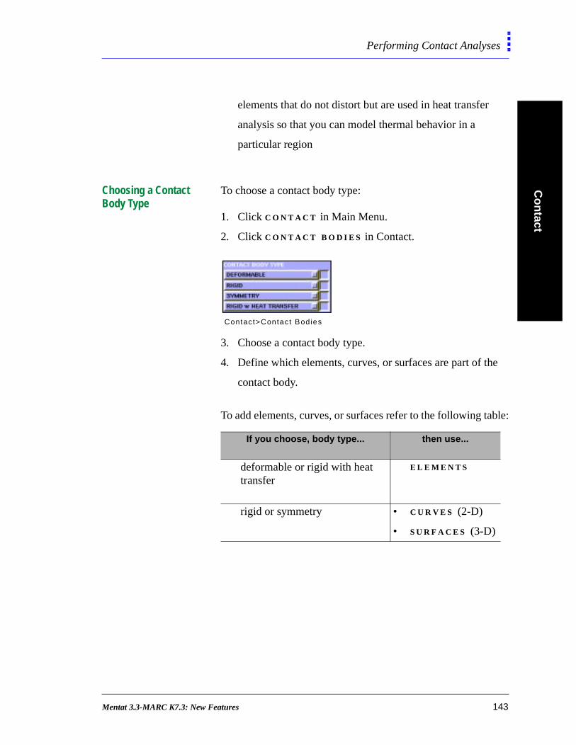
Co
ntact
Performing Contact Analyses
elements that do not distort but are used in heat transfer
analysis so that you can model thermal behavior in a
particular region
Choosing a Contact Body Type
To choose a contact body type:
1. Click C O N T A C T in Main Menu.
2. Click C O N T A C T B O D I E S in Contact.
3. Choose a contact body type.
4. Define which elements, curves, or surfaces are part of the
contact body.
To add elements, curves, or surfaces refer to the following table:
Contact>Contact Bodies
If you choose, body type... then use...
deformable or rigid with heat transfer
E L E M E N T S
rigid or symmetry • C U R V E S (2-D)
• S U R F A C E S (3-D)
Mentat 3.3-MARC K7.3: New Features 143
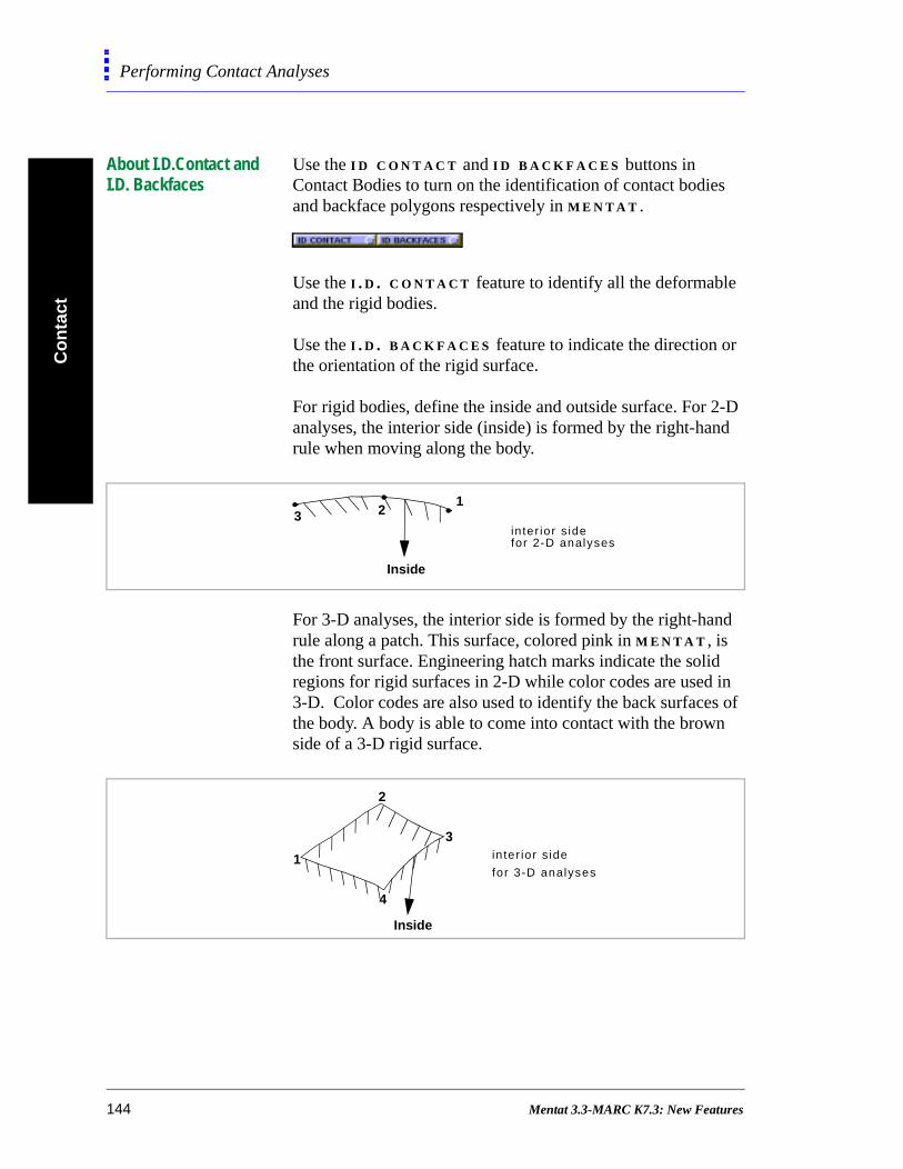
Co
nta
ctPerforming Contact Analyses
About I.D.Contact and I.D. Backfaces
Use the I D C O N T A C T and I D B A C K F A C E S buttons in Contact Bodies to turn on the identification of contact bodies and backface polygons respectively in M E N T A T .
Use the I . D . C O N T A C T feature to identify all the deformable and the rigid bodies.
Use the I . D . B A C K F A C E S feature to indicate the direction or the orientation of the rigid surface.
For rigid bodies, define the inside and outside surface. For 2-D analyses, the interior side (inside) is formed by the right-hand rule when moving along the body.
For 3-D analyses, the interior side is formed by the right-hand rule along a patch. This surface, colored pink in M E N T A T , is the front surface. Engineering hatch marks indicate the solid regions for rigid surfaces in 2-D while color codes are used in 3-D. Color codes are also used to identify the back surfaces of the body. A body is able to come into contact with the brown side of a 3-D rigid surface.
123
Inside
in ter ior s idefor 2-D analyses
1
4
3
2
Inside
in ter ior s ide
for 3-D analyses
144 Mentat 3.3-MARC K7.3: New Features

Co
ntact
Performing Contact Analyses
About Flip Elements, Curves, and Surfaces
If the surfaces on the contact bodies are not in the correct orientation, then, during the analysis procedure, a deformable body will penetrate a rigid surface.
Use the F L I P C U R V E S (2-D) or F L I P S U R F A C E S (3-D) buttons in Contact Bodies to correct the orientation of the contact bodies.
Finite Element Mesh for a Deformable Body
You can generate the finite element mesh for a deformable body using the mesh generation options in the Main Menu in M E N T A T .
Analysis Parameters for Deformable Bodies
The analysis parameters for deformable bodies are grouped under the following categories:
• Friction
• Description
• Heat Transfer Data for Coupled Analyses
Use the F R I C T I O N C O E F F I C I E N T option in Friction to associate a friction coefficient with a deformable body. You define the friction model in the J O B S option in Main Menu.
Use the Description field to prescribe how the surface of thedeformable body is represented in your contact analysis.
deformablebody
Mentat 3.3-MARC K7.3: New Features 145
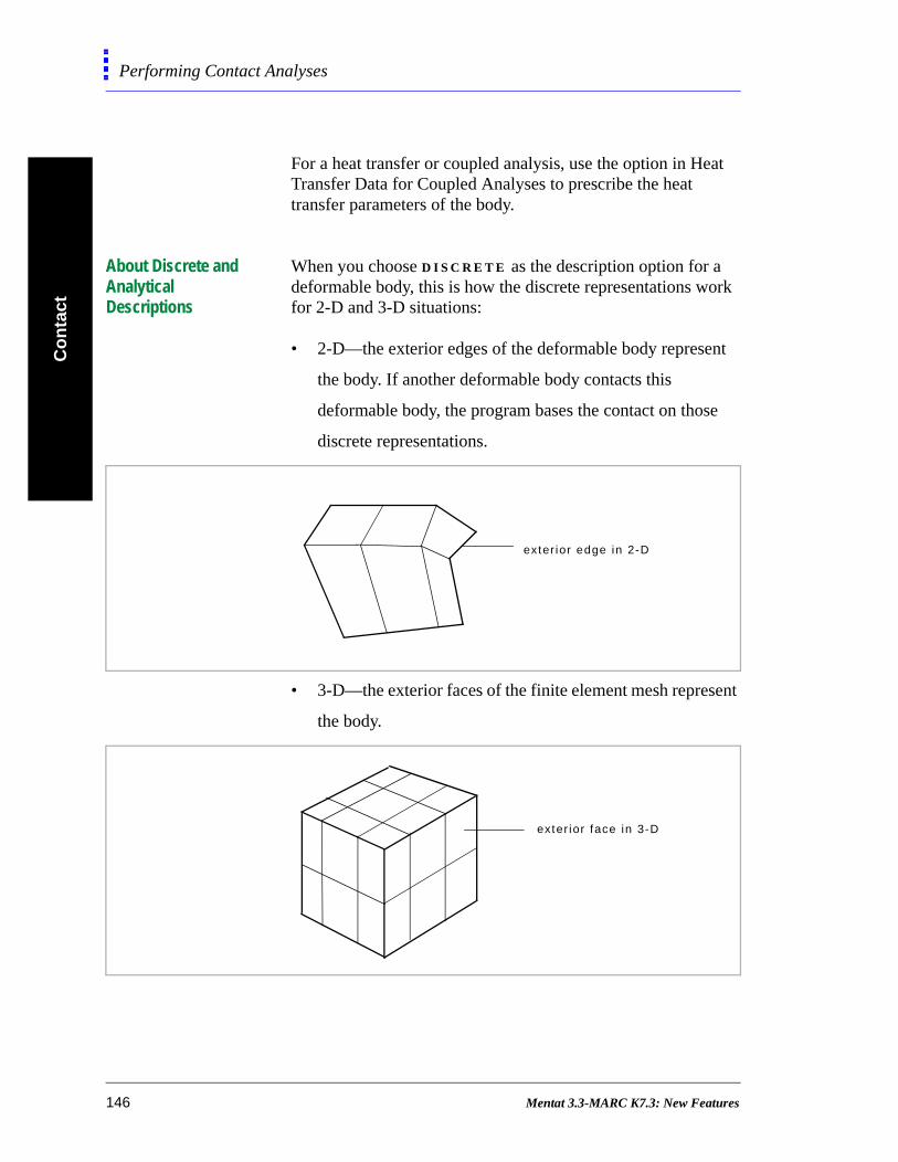
Co
nta
ctPerforming Contact Analyses
nt
e
ent
For a heat transfer or coupled analysis, use the option in Heat Transfer Data for Coupled Analyses to prescribe the heat transfer parameters of the body.
About Discrete and Analytical Descriptions
When you choose D I S C R E T E as the description option for a deformable body, this is how the discrete representations work for 2-D and 3-D situations:
• 2-D—the exterior edges of the deformable body represe
the body. If another deformable body contacts this
deformable body, the program bases the contact on thos
discrete representations.
• 3-D—the exterior faces of the finite element mesh repres
the body.
exter ior edge in 2-D
exter ior face in 3-D
146 Mentat 3.3-MARC K7.3: New Features
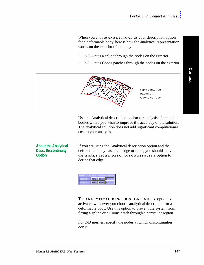
Co
ntact
Performing Contact Analyses
rior.
on. al
te
When you choose A N A L Y T I C A L as your description option for a deformable body, here is how the analytical representation works on the exterior of the body:
• 2-D—puts a spline through the nodes on the exterior.
• 3-D—puts Coons patches through the nodes on the exte
Use the Analytical description option for analysis of smooth bodies where you wish to improve the accuracy of the solutiThe analytical solution does not add significant computationcost to your analysis.
About the Analytical Desc. Discontinuity Option
If you are using the Analytical description option and the deformable body has a real edge or node, you should activathe A N A L Y T I C A L D E S C . D I S C O N T I N U I T Y option to define that edge.
The A N A L Y T I C A L D E S C . D I S C O N T I N U I T Y option is activated whenever you choose analytical description for a deformable body. Use this option to prevent the system fromfitting a spline or a Coons patch through a particular region.
For 2-D meshes, specify the nodes at which discontinuities occur.
representat ion
based on
Coons sur face
Mentat 3.3-MARC K7.3: New Features 147
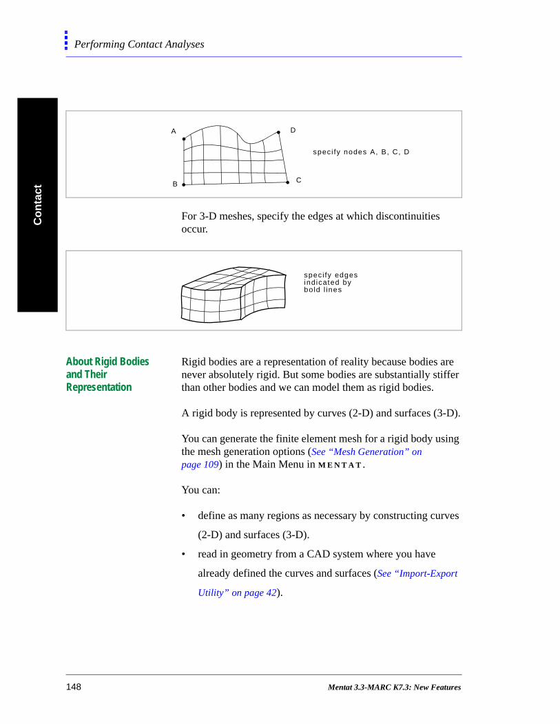
Co
nta
ctPerforming Contact Analyses
rves
For 3-D meshes, specify the edges at which discontinuities occur.
About Rigid Bodies and Their Representation
Rigid bodies are a representation of reality because bodies are never absolutely rigid. But some bodies are substantially stiffer than other bodies and we can model them as rigid bodies.
A rigid body is represented by curves (2-D) and surfaces (3-D).
You can generate the finite element mesh for a rigid body using the mesh generation options (See “Mesh Generation” on page 109) in the Main Menu in M E N T A T .
You can:
• define as many regions as necessary by constructing cu
(2-D) and surfaces (3-D).
• read in geometry from a CAD system where you have
already defined the curves and surfaces (See “Import-Export
Utility” on page 42).
speci fy nodes A, B, C, D
A
B C
D
specify edges indicated bybold l ines
148 Mentat 3.3-MARC K7.3: New Features

Co
ntact
Performing Contact Analyses
nd
Motion Control of Rigid Bodies
Use the following options to control the motion of a rigid body:
• velocity
• position
• force on the rigid surface (i.e., load)
To choose a motion control option for a rigid body:
1. Choose Contact>Contact Bodies.
2. Click R I G I D in Contact Body Type.
3. Choose a body control option.
About the Centroid and Rotation Axis Options
To control the motion of a rigid body, you associate a point aan axis with the rigid body using the C E N T R O I D and R O T A T I O N A X I S options in Rigid Body.
For 2-D analyses, you prescribe the x and y positions of thecentroid. For 3-D analyses, you prescribe the x, y, z, and therotational axis information.
Contact>Contact Bodies>Rig id
Contact>Contact Bodies>Rigid
Mentat 3.3-MARC K7.3: New Features 149
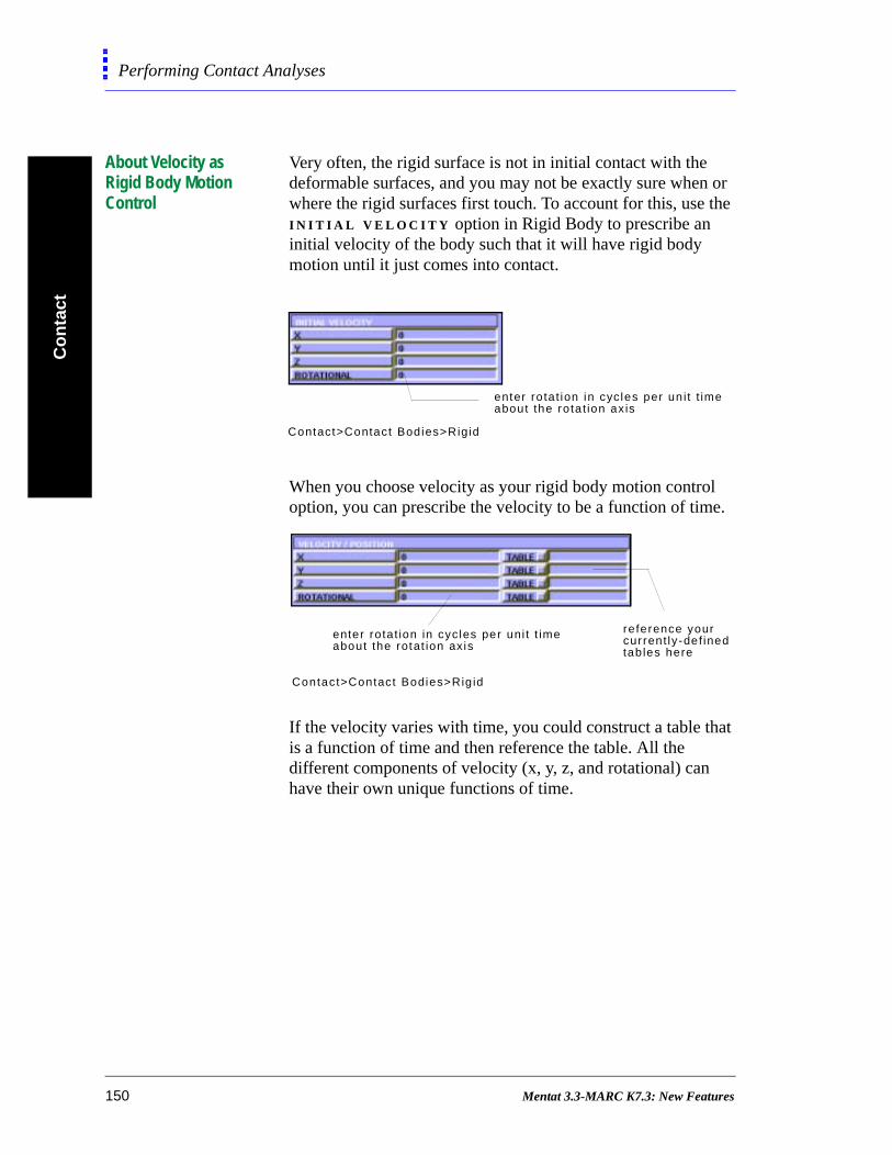
Co
nta
ctPerforming Contact Analyses
About Velocity as Rigid Body Motion Control
Very often, the rigid surface is not in initial contact with the deformable surfaces, and you may not be exactly sure when or where the rigid surfaces first touch. To account for this, use the I N I T I A L V E L O C I T Y option in Rigid Body to prescribe an initial velocity of the body such that it will have rigid body motion until it just comes into contact.
When you choose velocity as your rigid body motion control option, you can prescribe the velocity to be a function of time.
If the velocity varies with time, you could construct a table that is a function of time and then reference the table. All the different components of velocity (x, y, z, and rotational) can have their own unique functions of time.
enter ro ta t ion in cyc les per un i t t imeabout the rotat ion ax is
Contact>Contact Bodies>Rig id
reference yourcurrent ly-def inedtables here
enter rota t ion in cyc les per uni t t imeabout the rotat ion ax is
Contact>Contact Bodies>Rig id
150 Mentat 3.3-MARC K7.3: New Features
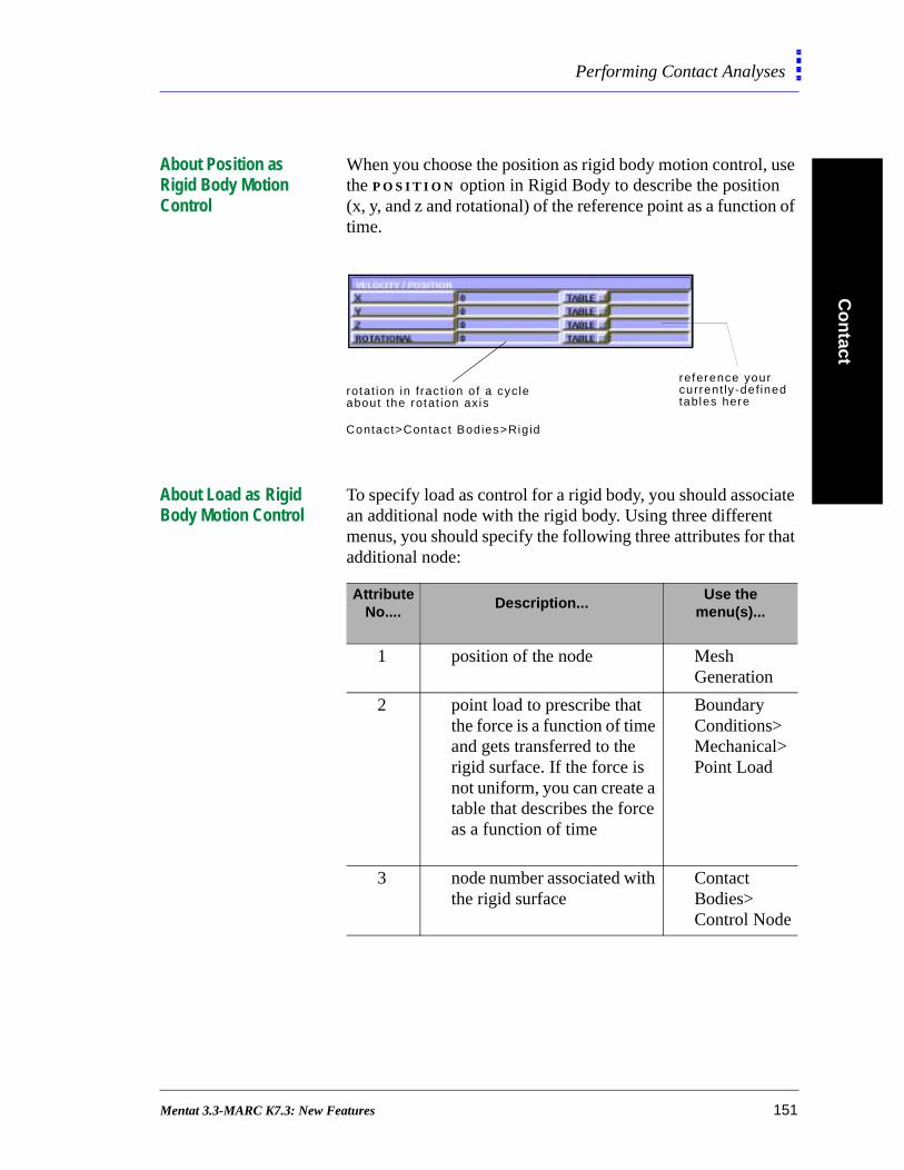
Co
ntact
Performing Contact Analyses
About Position as Rigid Body Motion Control
When you choose the position as rigid body motion control, use the P O S I T I O N option in Rigid Body to describe the position (x, y, and z and rotational) of the reference point as a function of time.
About Load as Rigid Body Motion Control
To specify load as control for a rigid body, you should associate an additional node with the rigid body. Using three different menus, you should specify the following three attributes for that additional node:
reference yourcurrent ly-def inedtables here
rotat ion in f ract ion of a cyc leabout the rotat ion ax is
Contact>Contact Bodies>Rig id
Attribute No....
Description...Use the
menu(s)...
1 position of the node Mesh Generation
2 point load to prescribe that the force is a function of time and gets transferred to the rigid surface. If the force is not uniform, you can create a table that describes the force as a function of time
Boundary Conditions> Mechanical>Point Load
3 node number associated with the rigid surface
Contact Bodies> Control Node
Mentat 3.3-MARC K7.3: New Features 151
Co
nta
ctPerforming Contact Analyses
Analytical and Discrete Description of Rigid Bodies
After you have defined the motion control parameters of the rigid body, you prescribe how the rigid surface is modeled numerically.
In M E N T A T , all surfaces are represented as NURB curves or NURB surfaces. For your contact analysis, you can decide whether to use the analytical (NURB) description of the rigid body or a discrete description of body. The default setting is the analytical description.
The analytical description is more accurate but results in higher computation cost per iteration. But in many problems, you might require fewer iterations when you use the analytical procedure.
Coupled Analysis Considerations
When you use rigid surfaces in a coupled analysis, the rigid surface is treated as a heat source or a heat sink. The rigid body is considered to be a fixed body of infinite mass so that the temperature does not change in it.
To set the parameters for heat transfer in a coupled analysis, use the Heat Transfer Data for Coupled Analysis area in Rigid Body.
To enter specific parameters for heat transfer in a coupled analysis, refer to the following table:
To prescribe... Use the button,...
the sink temperature of the rigid body
E N V I R O N M E N T S I N K T E M P E R A T U R E
how much of the temperature differential is going to result in a flux
C O N T A C T H E A T T R A N S F E R C O E F F .
152 Mentat 3.3-MARC K7.3: New Features
Co
ntact
Performing Contact Analyses
y
n
s
try
r
About Symmetry Bodies and Surfaces
Symmetry bodies are a subset of rigid bodies which have a unique behavior. Use symmetry surfaces when you have a body with a plane of symmetry associated with it.
In most cases, symmetry bodies are flat surfaces with a given orientation. You can model a given symmetry surface using either the analytical or discrete surface type. Symmetry surfaces are usually flat patches and you can use the analytical or discrete surface with little variance in results.
Special Assumptions for Symmetry Bodies
When you use a symmetry body, you make the following assumptions:
• the deformable body is in contact with the symmetry bod
from the beginning to the end of analysis. This assumptio
is necessary to maintain that there are no cracks or hole
generated during the analysis.
• the symmetry bodies are frictionless.
• there is no flux across a symmetry surface during a heat
transfer analysis (you don’t need to provide any thermal
information associated with a symmetry line or a symme
plane.).
About Rigid w/Heat Transfer Bodies
The analysis considerations for rigid bodies with heat transfeare very similar to considerations for a rigid body (See “About Rigid Bodies and Their Representation” on page 148)
For the motion control of a rigid body with heat transfer, you can prescribe the velocity or position only. You cannot prescribe a load (force) to the region.
Mentat 3.3-MARC K7.3: New Features 153

Co
nta
ctPerforming Contact Analyses
n
f nal
About Contact Tables Use the Contact Tables options in M E N T A T to determine the location of potential contact. By identifying a new contact table, you can indicate which body is potentially going to contact another body.
The Contact Table option is a very flexible way to enter complex contact conditions. You can use contact tables to specify that two bodies have particular attributes that are not shared with other pairs of contact bodies. These attributes include:
• contact distance
• separation force
• friction coefficient
• interface closure distance
Table Properties of a Contact Table
The T A B L E P R O P E R T I E S feature in Contact Tables is a flexible way to specify individual contact relationships betweebodies.
Use the contact tables in your analysis to determine areas opotential contact which can help you reduce your computatiocosts. You can specify any of the following conditions:
• every body potentially touches every other body.
• every body touches every other body but does not touch
itself.
• a body touches selected other bodies.
• a body is glued to another (or other) body (or bodies).
enter tab le proper t ies here
Contact>Contact Tables
154 Mentat 3.3-MARC K7.3: New Features
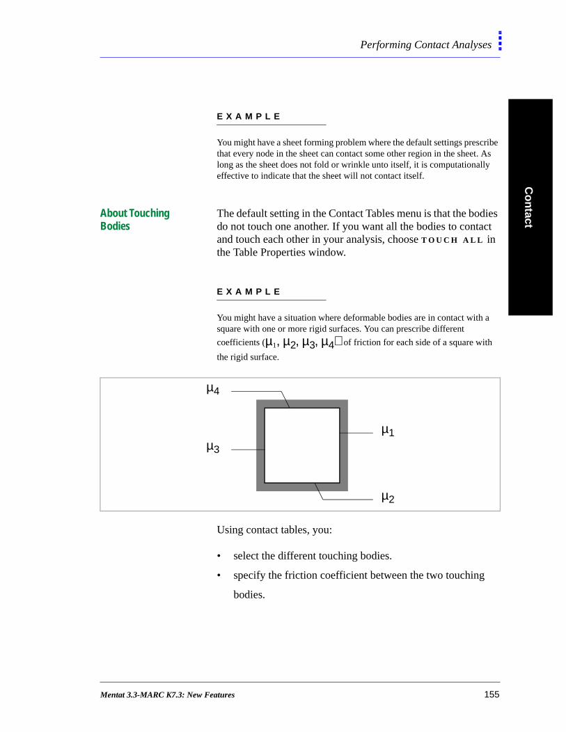
Co
ntact
Performing Contact Analyses
E X A M P L E
You might have a sheet forming problem where the default settings prescribe that every node in the sheet can contact some other region in the sheet. As long as the sheet does not fold or wrinkle unto itself, it is computationally effective to indicate that the sheet will not contact itself.
About Touching Bodies
The default setting in the Contact Tables menu is that the bodies do not touch one another. If you want all the bodies to contact and touch each other in your analysis, choose T O U C H A L L in the Table Properties window.
E X A M P L E
You might have a situation where deformable bodies are in contact with a square with one or more rigid surfaces. You can prescribe different
coefficients (µ1, µ2, µ3, µ4) of friction for each side of a square with
the rigid surface.
Using contact tables, you:
• select the different touching bodies.
• specify the friction coefficient between the two touching
bodies.
µ1
µ4
µ2
µ3
Mentat 3.3-MARC K7.3: New Features 155
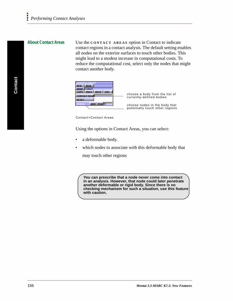
Co
nta
ctPerforming Contact Analyses
About Contact Areas Use the C O N T A C T A R E A S option in Contact to indicate contact regions in a contact analysis. The default setting enables all nodes on the exterior surfaces to touch other bodies. This might lead to a modest increase in computational costs. To reduce the computational cost, select only the nodes that might contact another body.
Using the options in Contact Areas, you can select:
• a deformable body.
• which nodes to associate with this deformable body that
may touch other regions
choose a body f rom the l is t o f current ly-def ined bodies
choose nodes in the body thatpotent ial ly touch other reg ions
Contact>Contact Areas
.
You can prescribe that a node never come into contactin an analysis. However, that node could later penetrateanother deformable or rigid body. Since there is nochecking mechanism for such a situation, use this featurewith caution.
156 Mentat 3.3-MARC K7.3: New Features
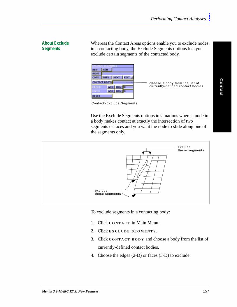
Co
ntact
Performing Contact Analyses
About Exclude Segments
Whereas the Contact Areas options enable you to exclude nodes in a contacting body, the Exclude Segments options lets you exclude certain segments of the contacted body.
Use the Exclude Segments options in situations where a node in a body makes contact at exactly the intersection of two segments or faces and you want the node to slide along one of the segments only.
To exclude segments in a contacting body:
1. Click C O N T A C T in Main Menu.
2. Click E X C L U D E S E G M E N T S .
3. Click C O N T A C T B O D Y and choose a body from the list of
currently-defined contact bodies.
4. Choose the edges (2-D) or faces (3-D) to exclude.
choose a body f rom the l is t o f current ly-def ined contact bodies
Contact>Exclude Segments
excludethese segments
excludethese segments
Mentat 3.3-MARC K7.3: New Features 157
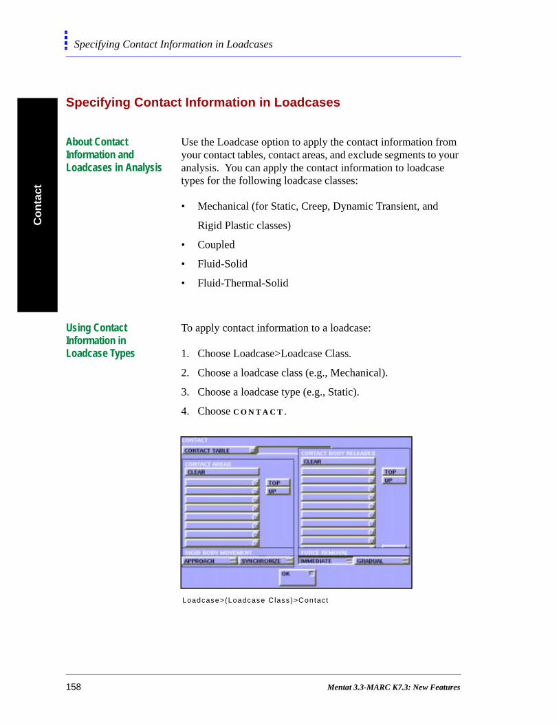
Co
nta
ctSpecifying Contact Information in Loadcases
Specifying Contact Information in Loadcases
About Contact Information and Loadcases in Analysis
Use the Loadcase option to apply the contact information from your contact tables, contact areas, and exclude segments to your analysis. You can apply the contact information to loadcase types for the following loadcase classes:
• Mechanical (for Static, Creep, Dynamic Transient, and
Rigid Plastic classes)
• Coupled
• Fluid-Solid
• Fluid-Thermal-Solid
Using Contact Information in Loadcase Types
To apply contact information to a loadcase:
1. Choose Loadcase>Loadcase Class.
2. Choose a loadcase class (e.g., Mechanical).
3. Choose a loadcase type (e.g., Static).
4. Choose C O N T A C T .
Loadcase>(Loadcase Class)>Contact
158 Mentat 3.3-MARC K7.3: New Features
Co
ntact
Specifying Contact Information in Loadcases
5. Choose from the list of contact tables and areas that you
defined.
About Contact Body Release
It is often useful to release nodes which are in contact with another body. A typical example would be when the rigid dies in a sheet forming process are removed from the sheet. When this occurs, the forces that were on a deformable body must be eliminated because the surface is now free. This results in a distribution of stress (in sheet forming, it results in spring back). It may also lead to a poor convergence if the forces are all removed at once. You can prevent this by removing the forces gradually using the G R A D U A L option in the Contact menu.
Using Contact Body Releases
To release nodes that are in contact with another body:
1. In the Contact menu, select the body from which the nodes
are to be separated.
2. Choose a type of release, I M M E D I A T E or G R A D U A L .
Preventing Separated Nodes from Contacting Again
After a node separates from a body, it may re-contact the same body. You can prevent this by using the Contact Table option to specify that the nodes cannot contact the body that they have been separated from. As an alternative approach, you can prescribe a time-dependent velocity or position to the surface such that it moves away from the nodes that have been separated from it.
. In a loadcase, you can have only one contact table
active; you can also activate multiple contact areas.
Mentat 3.3-MARC K7.3: New Features 159
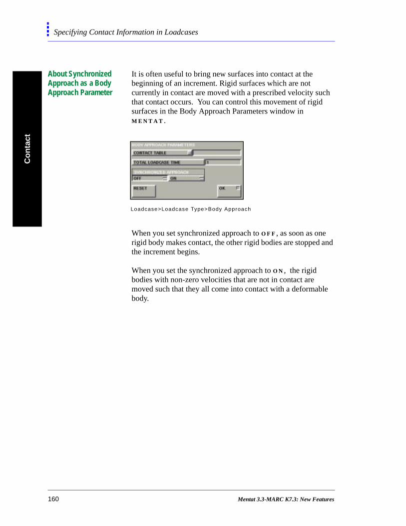
Co
nta
ctSpecifying Contact Information in Loadcases
About Synchronized Approach as a Body Approach Parameter
It is often useful to bring new surfaces into contact at the beginning of an increment. Rigid surfaces which are not currently in contact are moved with a prescribed velocity such that contact occurs. You can control this movement of rigid surfaces in the Body Approach Parameters window in M E N T A T .
When you set synchronized approach to O F F , as soon as one rigid body makes contact, the other rigid bodies are stopped and the increment begins.
When you set the synchronized approach to O N , the rigid bodies with non-zero velocities that are not in contact are moved such that they all come into contact with a deformable body.
Loadcase>Loadcase Type>Body Approach
160 Mentat 3.3-MARC K7.3: New Features
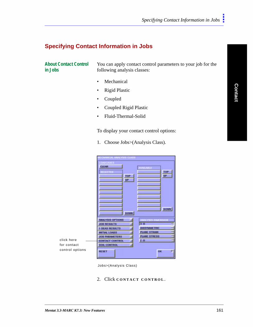
Co
ntact
Specifying Contact Information in Jobs
Specifying Contact Information in Jobs
About Contact Control in Jobs
You can apply contact control parameters to your job for the following analysis classes:
• Mechanical
• Rigid Plastic
• Coupled
• Coupled Rigid Plastic
• Fluid-Thermal-Solid
To display your contact control options:
1. Choose Jobs>(Analysis Class).
2. Click C O N T A C T C O N T R O L .
cl ick here
for contact
contro l opt ions
Jobs>(Analys is Class)
Mentat 3.3-MARC K7.3: New Features 161

Co
nta
ctSpecifying Contact Information in Jobs
s
n
About User Subroutines
Use the User Subroutine options in Contact Control to determine which user subroutines to activate in your contact analysis.
You can use one or more of the following user subroutines in your contact analysis:
• M O T I O N —prescribe either the velocity of the rigid
surfaces or the position of the rigid surfaces.
• S E P F O R — specify the force required for separation.
• S E P S T R —prescribe the stress required for separation.
• U C O N T A C T —prescribe your own contact procedure.
• U F R I C (an alternative to specifying the coefficient of
friction)—use in problems where friction coefficient is a
function of the pressures between the bodies or if the
friction coefficient was a function of the surface roughnes
and varied over the deformable region.
• U H T C O E —prescribe the heat transfer coefficient betwee
the deformable body and the environment and the
temperature of the environment.
• U H T C O N —specify, in coupled analyses, the thermal
coefficient between two bodies that are in contact.
Jobs>(Analys is Class)>Contact Contro l
162 Mentat 3.3-MARC K7.3: New Features
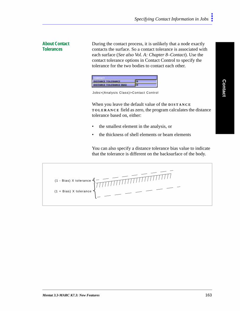
Co
ntact
Specifying Contact Information in Jobs
ate .
About Contact Tolerances
During the contact process, it is unlikely that a node exactly contacts the surface. So a contact tolerance is associated with each surface (See also Vol. A: Chapter 8–Contact). Use the contact tolerance options in Contact Control to specify the tolerance for the two bodies to contact each other.
When you leave the default value of the D I S T A N C E T O L E R A N C E field as zero, the program calculates the distance tolerance based on, either: • the smallest element in the analysis, or
• the thickness of shell elements or beam elements
You can also specify a distance tolerance bias value to indicthat the tolerance is different on the backsurface of the body
Jobs>(Analys is Class)>Contact Control
(1 - B ias) X to lerance
(1 + Bias) X to lerance
Mentat 3.3-MARC K7.3: New Features 163
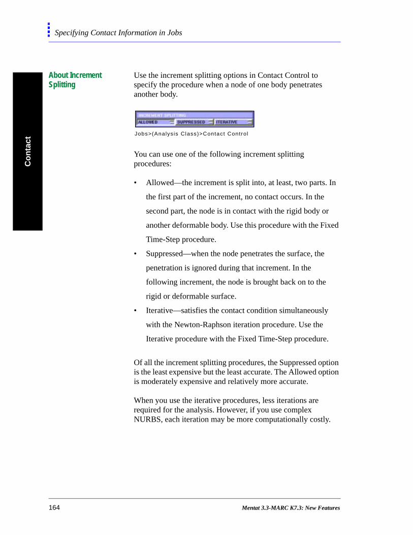
Co
nta
ctSpecifying Contact Information in Jobs
ed
tion tion
About Increment Splitting
Use the increment splitting options in Contact Control to specify the procedure when a node of one body penetrates another body.
You can use one of the following increment splitting procedures:
• Allowed—the increment is split into, at least, two parts. In
the first part of the increment, no contact occurs. In the
second part, the node is in contact with the rigid body or
another deformable body. Use this procedure with the Fix
Time-Step procedure.
• Suppressed—when the node penetrates the surface, the
penetration is ignored during that increment. In the
following increment, the node is brought back on to the
rigid or deformable surface.
• Iterative—satisfies the contact condition simultaneously
with the Newton-Raphson iteration procedure. Use the
Iterative procedure with the Fixed Time-Step procedure.
Of all the increment splitting procedures, the Suppressed opis the least expensive but the least accurate. The Allowed opis moderately expensive and relatively more accurate.
When you use the iterative procedures, less iterations are required for the analysis. However, if you use complex NURBS, each iteration may be more computationally costly.
Jobs>(Analys is Class)>Contact Control
164 Mentat 3.3-MARC K7.3: New Features

Co
ntact
Specifying Contact Information in Jobs
to
ntact
About Deformable-Deformable Contact Control
The default setting in the Deformable-Deformable option is such that when you use single-sided contact, a node on the lowered-numbered body is checked for contact with the segments on the higher-numbered body.
The body with the higher I.D. and the body with the lower I.D. are termed master body and slave body respectively. If you choose S I N G L E - S I D E D , then there is contact between the master body and the slave body. The Single-Sided option can often reduce your computational cost.
About Separation Procedures
Separation of a node with a body in M A R C is based upon either of the following procedures:
• nodal forces
• nodal stress
To use the S E P A R A T I O N F O R C E button based on forces or onstresses, refer to the following table:
In theory, separation occurs when there is a positive tensile force. However, from a numerical perspective, you may wishprescribe a large separation force. If you give too small a separation force, you might be faced with a higher computational cost because the nodes separate, return to coand separate again.
If you choose a separation procedure based on...
then, use the S E P A R A T I O N F O R C E button to enter the...
forces force at which two bodies separate.
stresses stress at which separation occurs.
Mentat 3.3-MARC K7.3: New Features 165
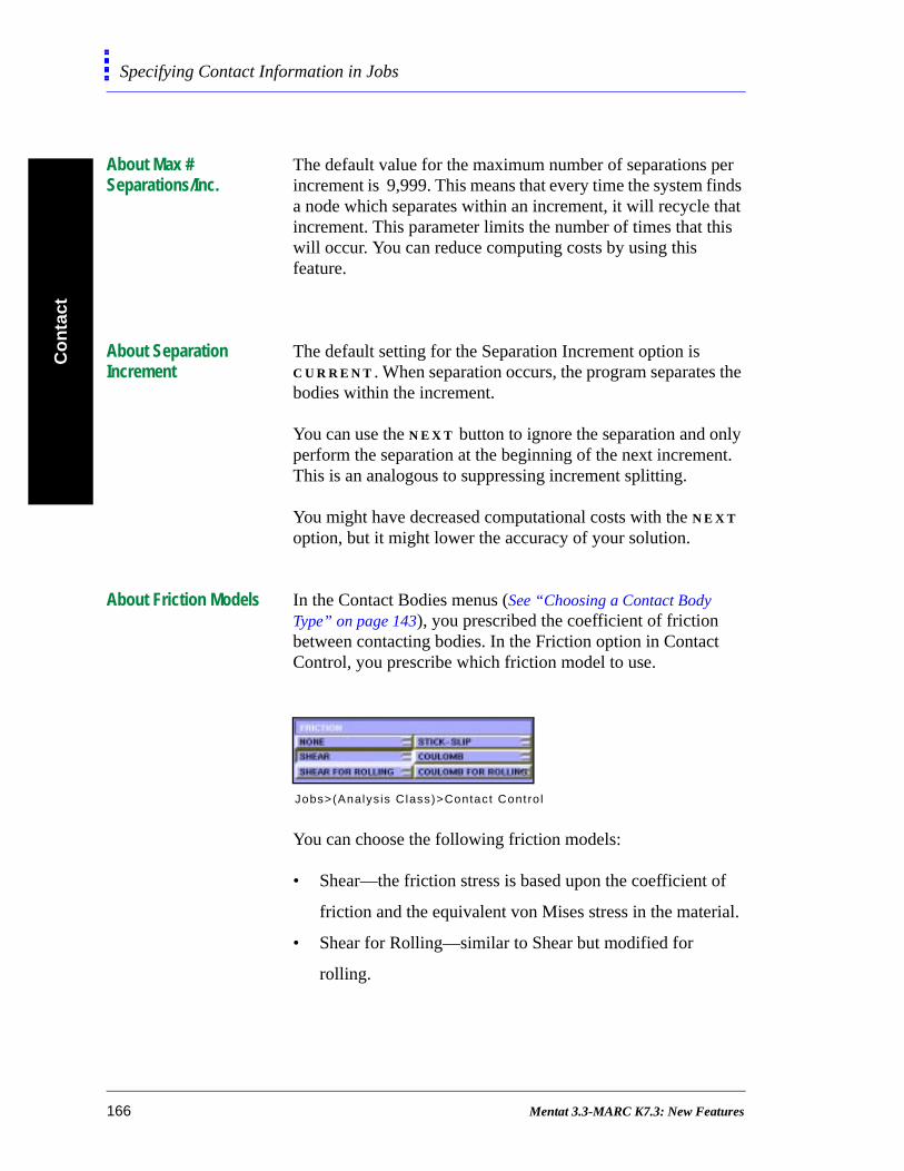
Co
nta
ctSpecifying Contact Information in Jobs
f
al.
About Max # Separations/Inc.
The default value for the maximum number of separations per increment is 9,999. This means that every time the system finds a node which separates within an increment, it will recycle that increment. This parameter limits the number of times that this will occur. You can reduce computing costs by using this feature.
About Separation Increment
The default setting for the Separation Increment option is C U R R E N T . When separation occurs, the program separates the bodies within the increment.
You can use the N E X T button to ignore the separation and only perform the separation at the beginning of the next increment. This is an analogous to suppressing increment splitting.
You might have decreased computational costs with the N E X T option, but it might lower the accuracy of your solution.
About Friction Models In the Contact Bodies menus (See “Choosing a Contact Body Type” on page 143), you prescribed the coefficient of friction between contacting bodies. In the Friction option in Contact Control, you prescribe which friction model to use.
You can choose the following friction models:
• Shear—the friction stress is based upon the coefficient o
friction and the equivalent von Mises stress in the materi
• Shear for Rolling—similar to Shear but modified for
rolling.
Jobs>(Analys is Class)>Contact Cont ro l
166 Mentat 3.3-MARC K7.3: New Features
Co
ntact
Specifying Contact Information in Jobs
t
• Coulomb—the friction stress is based upon the coefficienof friction and the normal stress at the surface.
• Coulomb for Rolling
• Stick-Slip
If you specify any of the friction models other than the Stick-Slip model, you have to specify the relative sliding velocity.
You also choose which of the following methods to use:
• Nodal Stress
• Nodal Force
E X C E P T I O N S :
Refer to the following table for exceptions:
For... the program uses this method...
Shear or Shear for Rolling models
Nodal Stress
Shell elements Nodal Force
Stick-Slip model Nodal Force
Mentat 3.3-MARC K7.3: New Features 167
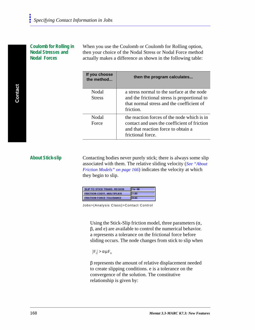
Co
nta
ctSpecifying Contact Information in Jobs
Coulomb for Rolling in Nodal Stresses and Nodal Forces
When you use the Coulomb or Coulomb for Rolling option, then your choice of the Nodal Stress or Nodal Force method actually makes a difference as shown in the following table:
About Stick-slip Contacting bodies never purely stick; there is always some slip associated with them. The relative sliding velocity (See “About Friction Models” on page 166) indicates the velocity at which they begin to slip.
Using the Stick-Slip friction model, three parameters (α, β, and e) are available to control the numerical behavior. a represents a tolerance on the frictional force before sliding occurs. The node changes from stick to slip when
β represents the amount of relative displacement needed to create slipping conditions. e is a tolerance on the convergence of the solution. The constitutive relationship is given by:
If you choose the method...
then the program calculates...
Nodal Stress
a stress normal to the surface at the node and the frictional stress is proportional to that normal stress and the coefficient of friction.
Nodal Force
the reaction forces of the node which is in contact and uses the coefficient of friction and that reaction force to obtain a frictional force.
Jobs>(Analys is Class)>Contact Contro l
Ft αµFn>
168 Mentat 3.3-MARC K7.3: New Features
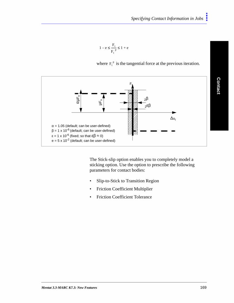
Co
ntact
Specifying Contact Information in Jobs
where is the tangential force at the previous iteration.
The Stick-slip option enables you to completely model a sticking option. Use the option to prescribe the following parameters for contact bodies:
• Slip-to-Stick to Transition Region
• Friction Coefficient Multiplier
• Friction Coefficient Tolerance
1 eFt
Ftp-------- 1 e+≤ ≤–
Ftp
µFn
αµF
n
Ft
2β
2εβ
∆ut
α = 1.05 (default; can be user-defined)β = 1 x 10⁻⁶ (default; can be user-defined)
ε = 1 x 10⁻⁶ (fixed; so that εβ ≈ 0)e = 5 x 10⁻² (default; can be user-defined)
Mentat 3.3-MARC K7.3: New Features 169
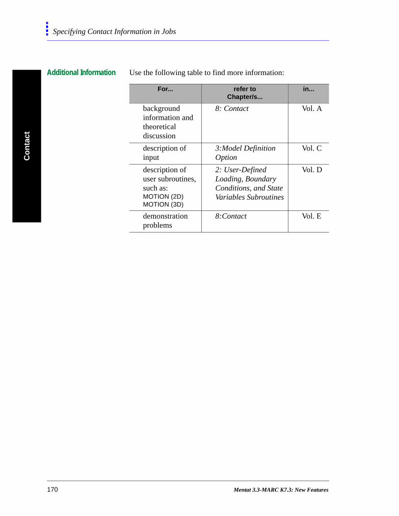
Co
nta
ctSpecifying Contact Information in Jobs
Additional Information Use the following table to find more information:
For... refer to Chapter/s...
in...
background information and theoretical discussion
8: Contact Vol. A
description of input
3:Model Definition Option
Vol. C
description of user subroutines, such as:MOTION (2D)MOTION (3D)
2: User-Defined Loading, Boundary Conditions, and State Variables Subroutines
Vol. D
demonstration problems
8:Contact Vol. E
170 Mentat 3.3-MARC K7.3: New Features
7• Design Sensitivity and Optimization
Design Sensitivity and Optimization
About Design Sensitivity and Optimization 173Application of Design Variables and Design Constraints to Jobs 175
Design Variables
Types of Design Variables 177About Bounds and Design Sensitivity 178
Design Constraints
Types of Constraints 182Setting Displacement Constraints 183
Using Design Variables and Constraints
Associating Constraints with a Loadcase 188
Post-Processing Sensitivity and OptimizationResults
About the Plotting of Sensitivity Results 194About History Plots of Optimization Results 201
Mentat 3.3-MARC K7.3: New Features 171
• Design Sensitivity and Optimization
Mentat 3.3-MARC K7.3: New Features
Desig
n S
ensitivity an
d O
ptim
ization
Design Sensitivity and Optimization
nd
ies
f
o
l
ss,
n
d to
Design Sensitivity and Optimization
About Design Sensitivity and Optimization
The relevant concepts relating to design optimization are:
• Analysis—evaluating the values of response quantities a
the objective function based on a given set of design
variable values.
• Sensitivity—evaluating the tendency of response quantit
to change with respect to the design variables.
Components of Design Optimization
The three components of design optimization that you can apply to design sensitivity and optimization jobs in M E N T A T are:
• Design Objective—either a direct or an indirect function o
design variables; currently, the design objective can be t
minimize the material mass, the volume, or the cost of a
structural design.
• Design Variables—quantifiable, variable parameters of
design. The design variable is associated with a physica
quantity of design that you can specify (e.g., shell thickne
Young’s modulus, material density, or composite ply
angles).
• Design Constraints—direct or indirect limitations on desig
variables or response quantities. The constraints are use
place bounds on design variables or impose limits on the
Mentat 3.3-MARC K7.3: New Features 173

Des
ign
Sen
siti
vity
an
d O
pti
miz
atio
nDesign Sensitivity and Optimization
e:
response. For example, you would constrain the response
such that a resultant stress (or deflection) is less than a
certain value.
In M E N T A T , the specification of design constraints and design variables is independent of the types of jobs. So, for example, you could specify several design variables or constraints and use only some of them in one job and others, including some of the previous ones, in another job.
When to Apply Design Optimization
Use the Design Optimization feature to:
• achieve a good approximation of the final design
• gauge the direction of the final design
Where You Can Apply Design Optimization
Use the Design Optimization feature in structures that involv
• static loads
• linear behavior
• multiple loadcases
• multiple constraints on stress, strain, and eigenfrequency
response
174 Mentat 3.3-MARC K7.3: New Features
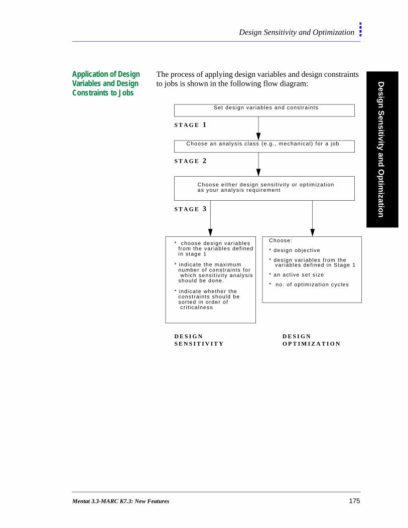
Desig
n S
ensitivity an
d O
ptim
ization
Design Sensitivity and Optimization
Application of Design Variables and Design Constraints to Jobs
The process of applying design variables and design constraints to jobs is shown in the following flow diagram:
Set des ign var iab les and constra in ts
Choose an analys is c lass (e.g. , mechanical) for a job
Choose e i ther des ign sensit iv i ty or opt im izat ion
Choose:
* design ob ject ive
* des ign var iab les f rom the var iables def ined in Stage 1
* an act ive set s ize
* no. o f opt im izat ion cyc les
as your analys is requirement
S T A G E 1
S T A G E 2
S T A G E 3
D E S I G N D E S I G NS E N S I T I V I T Y O P T I M I Z A T I O N
* choose design var iab les f rom the var iab les def ined in stage 1
* indicate the maximum number of constraints for which sensit iv i ty analys is should be done.
* indicate whether the constraints should be sor ted in order of c r i t ica lness
Mentat 3.3-MARC K7.3: New Features 175
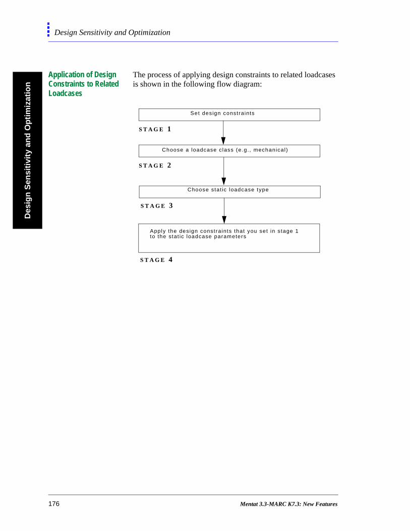
Des
ign
Sen
siti
vity
an
d O
pti
miz
atio
nDesign Sensitivity and Optimization
Application of Design Constraints to Related Loadcases
The process of applying design constraints to related loadcases is shown in the following flow diagram:
Set des ign constra ints
Choose a loadcase c lass (e.g. , mechanica l)
S T A G E 1
S T A G E 2
S T A G E 3
Choose stat ic loadcase type
Apply the design const raints that you set in s tage 1to the stat ic loadcase parameters
S T A G E 4
176 Mentat 3.3-MARC K7.3: New Features

Desig
n S
ensitivity an
d O
ptim
ization
Design Variables
yer. f
Design Variables
Types of Design Variables
You can use the following types of design variables in M E N T A T :
• material
• composite
• geometry
To pick a design variable type, choose D E S I G N V A R I A B L E S in the Main Menu.
Linking and Unlinking Design Variables
Use the L I N K E D feature to associate one geometry design variable with more than one entity, such as an element or laTo create geometry design variables that are independent oeach other, use U N L I N K E D .
E X A M P L E :
You can define plate thickness as a design variable. If you specify certain elements (say, 1-10) with the design variable and you choose L I N K E D , then all of the elements, 1-10, have the same thickness. When the program changes the value of plate thickness, the elements, 1-10, reflect that change.
Main Menu>Design Var iab les
pick a design var iab le
set a des ign space for the design var iab les
create l inked or independentdesign var iab les
Mentat 3.3-MARC K7.3: New Features 177

Des
ign
Sen
siti
vity
an
d O
pti
miz
atio
nDesign Variables
You can also use the linking options to specify that the ply angles or layer thicknesses of multiple layers should be the same.
When you use material design variables, the design variable for all elements associated with the chosen material are automatically linked.
About Bounds and Design Sensitivity
Use the L O W E R B O U N D and U P P E R B O U N D buttons to establish a design space for your design variables. The upper and lower bounds create a range for the design variables used in the optimization analysis.
Choosing tight bounds constrains the optimization, but, in general, leads to a faster analysis and a more accurate design.
Within the design space, you can pick certain points and perform sensitivity analyses at those points. The sensitivity analysis is performed using the prescribed values of the design variables. In an optimization analysis, these prescribed values are not relevant.
178 Mentat 3.3-MARC K7.3: New Features

Desig
n S
ensitivity an
d O
ptim
ization
Design Variables
Using Materials as Design Variables
To specify a material property as a design variable:
1. Choose Design Variables>Material.
2. Enter the upper and lower bound.
3. Use S E L M A T E R I A L to pick materials from the Currently
Defined Base MaterialS window.
Using Composites as Design Variables
Use the Composites option to define the design variables for a composite group.
The design variables for composites are:
Design Var iab les>Materia l
Design Var iab les>Composites
choose between layer th icknessand ply angle
use this but ton to associate the des ign var iab le with one or more layers.
Mentat 3.3-MARC K7.3: New Features 179
Des
ign
Sen
siti
vity
an
d O
pti
miz
atio
nDesign Variables
to one-u
• ply angle
• layer thickness
Use the S E L C O M P O S I T E button to choose a composite material to apply the design variables to.
Geometry Design Variables
The geometry design variables for design optimization relatethe element sizing parameters. These variables must have ato-one correspondence with the geometry constants that yodefine for each particular element.
E X A M P L E :
IXX and IYY are the moments of inertia along the X and Y axes respectively for beam elements. If an element does not have the moment of inertia defined in the geometry option, you cannot have it as a design variable for that element.
Types of Geometry Design Variables
You can also define the following variables as geometry variables:
• Area (cross-sectional area of a truss element or a beam
element)
• Beam height (also occurs as thickness in the element
library)
• Beam width
• Radius of hollow cross-sections
• Wall thickness of hollow cross-sections
• Constant thickness (for shells, plane stress elements,
membrane elements, generalized plane strain elements)
180 Mentat 3.3-MARC K7.3: New Features
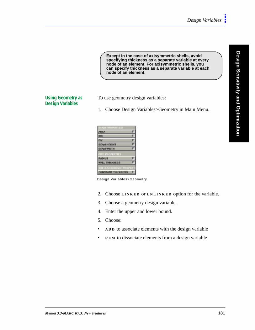
Desig
n S
ensitivity an
d O
ptim
ization
Design Variables
Using Geometry as Design Variables
To use geometry design variables:
1. Choose Design Variables>Geometry in Main Menu.
2. Choose L I N K E D or U N L I N K E D option for the variable.
3. Choose a geometry design variable.
4. Enter the upper and lower bound.
5. Choose:
• A D D to associate elements with the design variable
• R E M to dissociate elements from a design variable.
.
Except in the case of axisymmetric shells, avoidspecifying thickness as a separate variable at everynode of an element. For axisymmetric shells, youcan specify thickness as a separate variable at eachnode of an element.
Design Var iab les>Geometry
Mentat 3.3-MARC K7.3: New Features 181
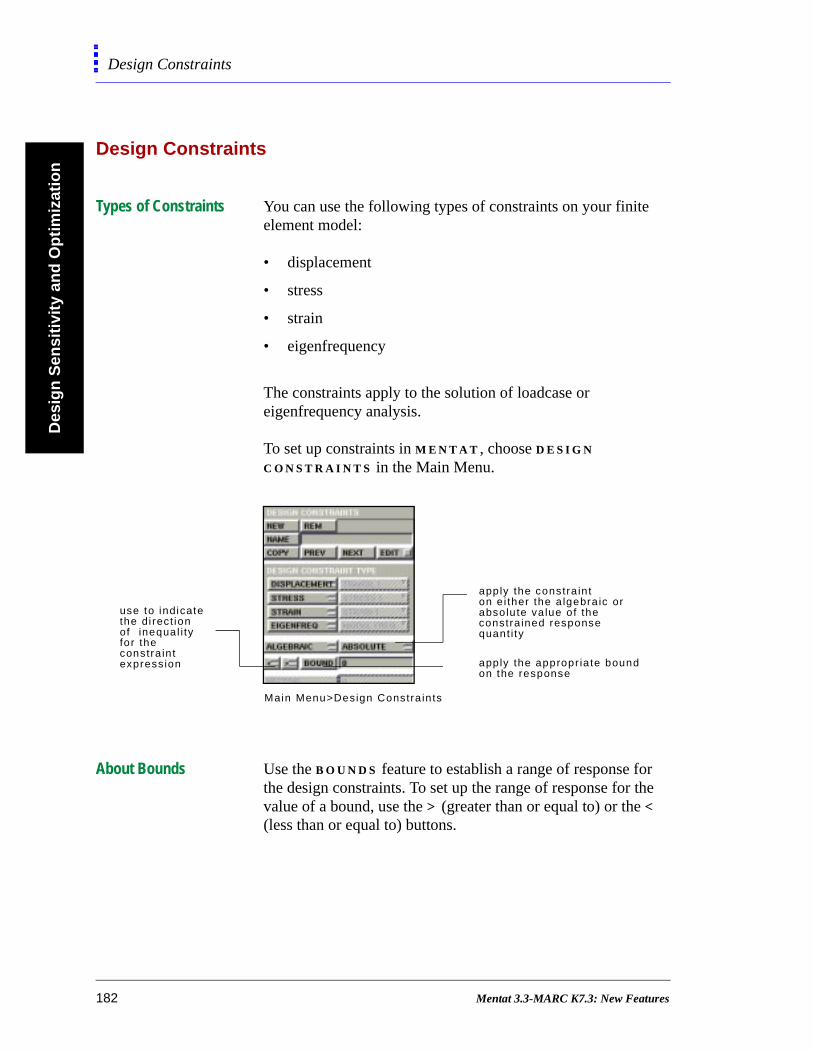
Des
ign
Sen
siti
vity
an
d O
pti
miz
atio
nDesign Constraints
he
Design Constraints
Types of Constraints You can use the following types of constraints on your finite element model:
• displacement
• stress
• strain
• eigenfrequency
The constraints apply to the solution of loadcase or eigenfrequency analysis.
To set up constraints in M E N T A T , choose D E S I G N C O N S T R A I N T S in the Main Menu.
About Bounds Use the B O U N D S feature to establish a range of response forthe design constraints. To set up the range of response for tvalue of a bound, use the > (greater than or equal to) or the < (less than or equal to) buttons.
Main Menu>Design Constra in ts
apply the constra in ton e i ther the a lgebra ic or absolute va lue of the constra ined response quant i ty
apply the appropr ia te boundon the response
use to indicatethe di rect ionof inequal i tyfor the constra in texpress ion
182 Mentat 3.3-MARC K7.3: New Features

Desig
n S
ensitivity an
d O
ptim
ization
Design Constraints
Algebraic and Absolute Values
To put a constraint on the algebraic value, choose the A L G E B R A I C feature. This feature gives you the flexibility to set bounds on both the positive and the negative sides.
A typical algebraic constant would be:
When you choose the A B S O L U T E button, the program picks the absolute, positive value of the response quantity.
A typical absolute value of constraint would be:
Setting Displacement Constraints
To set new displacement constraints:
1. Click D E S I G N C O N S T R A I N T S in the main menu.
2. Click D I S P L A C E M E N T .
3. Choose a constraint from the drop-down menu.
• For directed displacement constraints (e.g., directed
rotation), enter the vector direction/plane normal.
4. Enter the bounds information and assign a range.
Ux Umax<
σ σmax<
Design Constra in ts>Disp lacement
Mentat 3.3-MARC K7.3: New Features 183
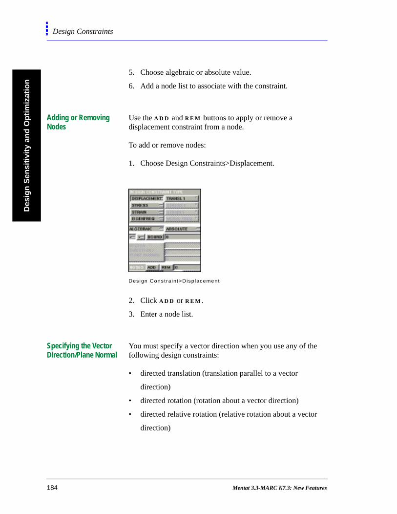
Des
ign
Sen
siti
vity
an
d O
pti
miz
atio
nDesign Constraints
5. Choose algebraic or absolute value.
6. Add a node list to associate with the constraint.
Adding or Removing Nodes
Use the A D D and R E M buttons to apply or remove a displacement constraint from a node.
To add or remove nodes:
1. Choose Design Constraints>Displacement.
2. Click A D D or R E M .
3. Enter a node list.
Specifying the Vector Direction/Plane Normal
You must specify a vector direction when you use any of the following design constraints:
• directed translation (translation parallel to a vector
direction)
• directed rotation (rotation about a vector direction)
• directed relative rotation (relative rotation about a vector
direction)
Design Constraint>Disp lacement
184 Mentat 3.3-MARC K7.3: New Features
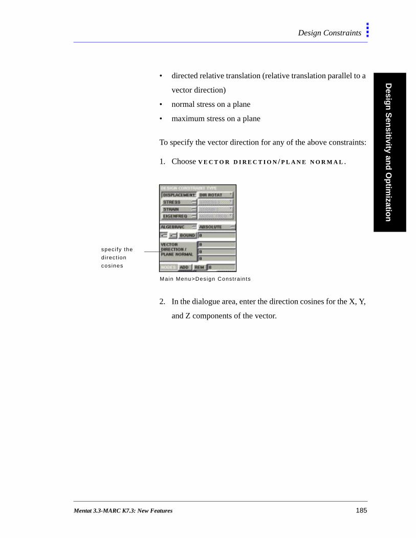
Desig
n S
ensitivity an
d O
ptim
ization
Design Constraints
a
ts:
, Y,
• directed relative translation (relative translation parallel to
vector direction)
• normal stress on a plane
• maximum stress on a plane
To specify the vector direction for any of the above constrain
1. Choose V E C T O R D I R E C T I O N / P L A N E N O R M A L .
2. In the dialogue area, enter the direction cosines for the X
and Z components of the vector.
Main Menu>Design Constra in ts
speci fy the
direct ion
cosines
Mentat 3.3-MARC K7.3: New Features 185
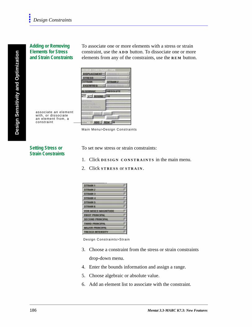
Des
ign
Sen
siti
vity
an
d O
pti
miz
atio
nDesign Constraints
Adding or Removing Elements for Stress and Strain Constraints
To associate one or more elements with a stress or strain constraint, use the A D D button. To dissociate one or more elements from any of the constraints, use the R E M button.
Setting Stress or Strain Constraints
To set new stress or strain constraints:
1. Click D E S I G N C O N S T R A I N T S in the main menu.
2. Click S T R E S S or S T R A I N .
3. Choose a constraint from the stress or strain constraints
drop-down menu.
4. Enter the bounds information and assign a range.
5. Choose algebraic or absolute value.
6. Add an element list to associate with the constraint.
associate an elementwi th, or dissociatean e lement f rom, aconstrain t
Main Menu>Design Constra in ts
Design Constra in ts>Stra in
186 Mentat 3.3-MARC K7.3: New Features
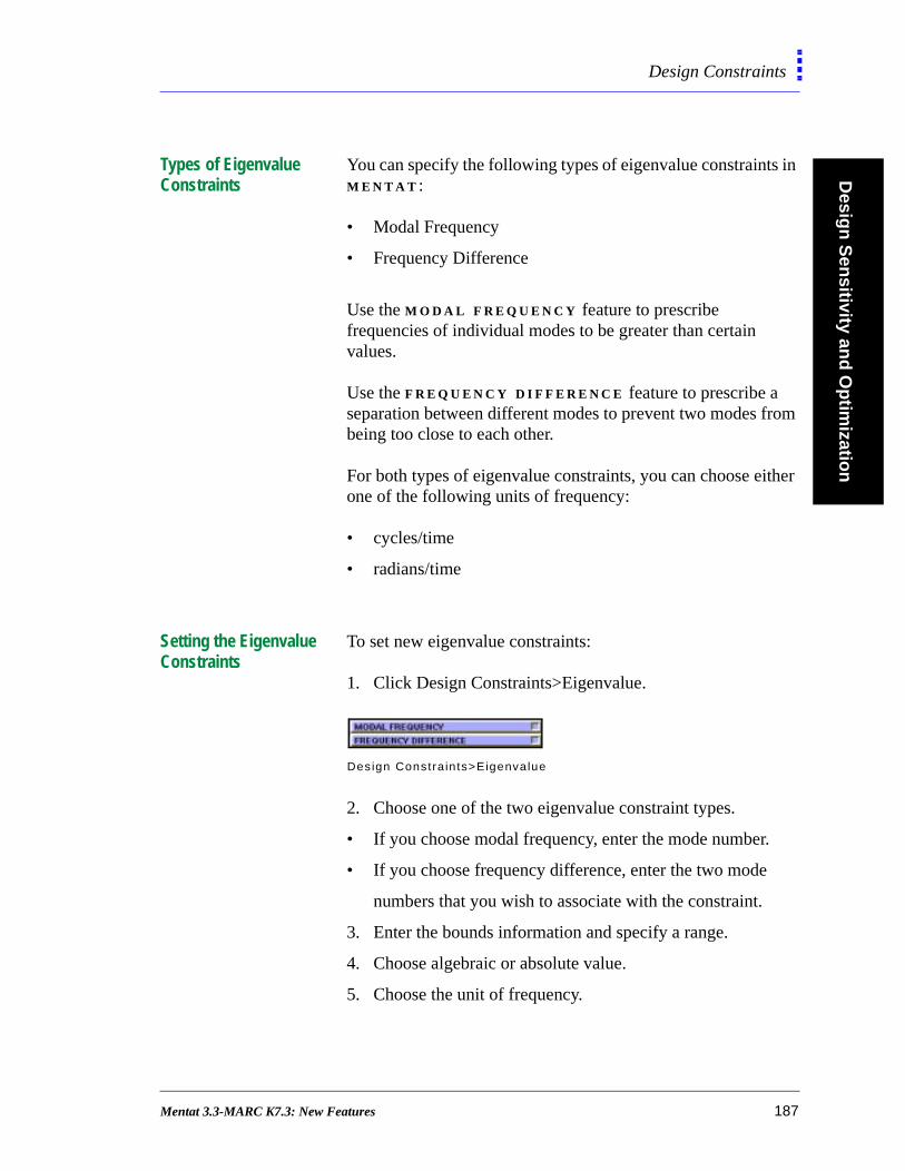
Desig
n S
ensitivity an
d O
ptim
ization
Design Constraints
om
ther
Types of Eigenvalue Constraints
You can specify the following types of eigenvalue constraints in M E N T A T :
• Modal Frequency
• Frequency Difference
Use the M O D A L F R E Q U E N C Y feature to prescribe frequencies of individual modes to be greater than certain values.
Use the F R E Q U E N C Y D I F F E R E N C E feature to prescribe a separation between different modes to prevent two modes frbeing too close to each other.
For both types of eigenvalue constraints, you can choose eione of the following units of frequency:
• cycles/time
• radians/time
Setting the Eigenvalue Constraints
To set new eigenvalue constraints:
1. Click Design Constraints>Eigenvalue.
2. Choose one of the two eigenvalue constraint types.
• If you choose modal frequency, enter the mode number.
• If you choose frequency difference, enter the two mode
numbers that you wish to associate with the constraint.
3. Enter the bounds information and specify a range.
4. Choose algebraic or absolute value.
5. Choose the unit of frequency.
Design Constra in ts>Eigenvalue
Mentat 3.3-MARC K7.3: New Features 187
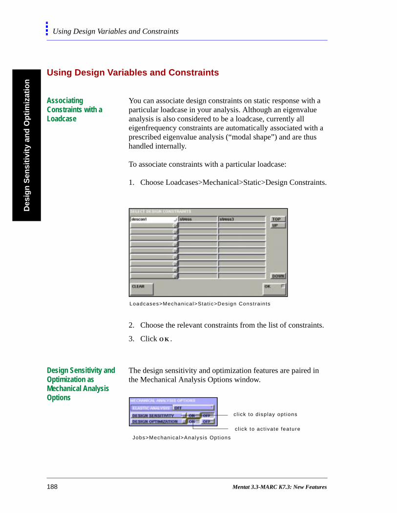
Des
ign
Sen
siti
vity
an
d O
pti
miz
atio
nUsing Design Variables and Constraints
s
ints.
ts.
n
Using Design Variables and Constraints
Associating Constraints with a Loadcase
You can associate design constraints on static response with a particular loadcase in your analysis. Although an eigenvalue analysis is also considered to be a loadcase, currently all eigenfrequency constraints are automatically associated with a prescribed eigenvalue analysis (“modal shape”) and are thuhandled internally.
To associate constraints with a particular loadcase:
1. Choose Loadcases>Mechanical>Static>Design Constra
2. Choose the relevant constraints from the list of constrain
3. Click O K .
Design Sensitivity and Optimization as Mechanical Analysis Options
The design sensitivity and optimization features are paired ithe Mechanical Analysis Options window.
Loadcases>Mechanica l>Stat ic>Design Constra in ts
c l ick to d isp lay opt ions
cl ick to act ivate feature
Jobs>Mechanica l>Analys is Opt ions
188 Mentat 3.3-MARC K7.3: New Features
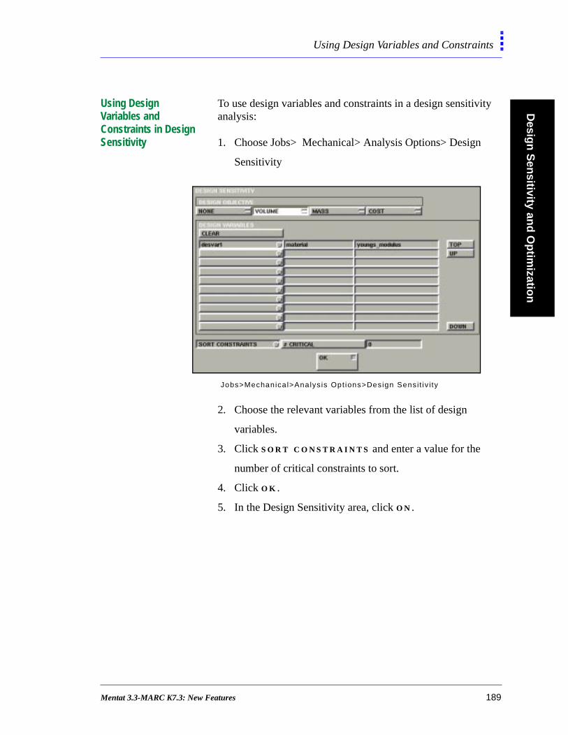
Desig
n S
ensitivity an
d O
ptim
ization
Using Design Variables and Constraints
Using Design Variables and Constraints in Design Sensitivity
To use design variables and constraints in a design sensitivity analysis:
1. Choose Jobs> Mechanical> Analysis Options> Design
Sensitivity
2. Choose the relevant variables from the list of design
variables.
3. Click S O R T C O N S T R A I N T S and enter a value for the
number of critical constraints to sort.
4. Click O K .
5. In the Design Sensitivity area, click O N .
Jobs>Mechanica l>Analys is Opt ions>Design Sensit iv i ty
Mentat 3.3-MARC K7.3: New Features 189

Des
ign
Sen
siti
vity
an
d O
pti
miz
atio
nUsing Design Variables and Constraints
Design Objective Considerations
If your design objective is mass, then you should provide the material unit mass for each of the elements.
You can specify the cost of a material as either of the following:
• per unit volume
• per unit mass
.
When you prepare the material data, remember to providethe material cost per unit mass or volume. If your materialdata is per unit mass, then you should also provide themass density of the material.
190 Mentat 3.3-MARC K7.3: New Features

Desig
n S
ensitivity an
d O
ptim
ization
Using Design Variables and Constraints
Using Design Variables in Design Optimization
To use design variables in design optimization analysis:
1. Choose Jobs>Mechanical>Analysis Options>Design
Optimization.
2. Choose a design objective.
3. Choose the relevant variables from the list of design
variables.
4. Enter a constraint set size or use the default set size.
5. Enter the number of cycles or use the default number of
cycles.
6. Click O K .
About Maximum Active Set Size
Use the M A X . A C T I V E S E T S I Z E feature to work with a certain size of a constraint set. The constraint set determines the maximum number of constraints for sensitivity analysis during optimization.
Jobs>Mechanical>Analys is Opt ions>Design Opt imizat ion
Mentat 3.3-MARC K7.3: New Features 191

Des
ign
Sen
siti
vity
an
d O
pti
miz
atio
nUsing Design Variables and Constraints
The default set size is 100. You can alter the size of the active set to obtain the best results for your design optimization job. The larger the size of the active constraint set, the greater the computational costs.
About Maximum Cycles
A cycle comprises of an exact analysis and a completed cycle of design iteration. The default number of cycles is 20. You can alter the number of cycles depending on your:
• optimization results
• computational resources
192 Mentat 3.3-MARC K7.3: New Features

Desig
n S
ensitivity an
d O
ptim
ization
Using Design Variables and Constraints
Additional Information Use the following table to find more information:
For... refer to Chapter/s...
in...
definitions of individual buttons
10: Design Variables and Constraints
Mentat 3.1 Command Reference
background information and theoretical discussion
5: Structural Procedure Library
Vol. A
description of design sensitivity and design optimization parameters
2:Parameters Vol. C
description of the following options:
• DESIGN OBJECTIVE• DESIGN VARIABLES• DESIGN DISPLACE-
MENT• CONSTRAINTS• DESIGN STRESS
CONSTRAINTS• DESIGN STRAIN
CONSTRAINTS• DESIGN FRE-
QUENCY CON-STRAINTS
3: Model Definition Options–Program Control
Vol. C
list of demonstration problems
Appendix F: Demonstration Problems
this guide
Mentat 3.3-MARC K7.3: New Features 193
Des
ign
Sen
siti
vity
an
d O
pti
miz
atio
nPost-Processing of Sensitivity Results
Post-Processing of Sensitivity Results
About the Plotting of Sensitivity Results
In plotting of the results of a sensitivity analysis, the increment number associated with the plot is one increment higher than the highest increment number relating to loadcases. E X A M P L E
Under the M A R C increment numbering system, if there are three static analyses (the program does not count the eigenvalue analysis as an increment), the system adds one to that number. So all the sensitivity-related plots are shown as sub-increments of a fourth increment number.
When you read in the M A R C post file of the sensitivity results in M E N T A T , the program displays the last available increment in the post file. Each of the responses is a sub-increment, starting from first to the nth sub-increment. The only exception is the objective function, which, if it exists, appears in the zeroth sub-increment.
About Constraint Reference Numbers
The sub-increment numbers for sensitivity analysis have a one-to-one correspondence with the constraint reference numbers in the output file for sensitivity results. A constraint reference number is a unique number associated with a response for which a sensitivity analysis is done. Therefore, for this particular increment, the sub-increment numbers are neither necessarily contiguous nor in increasing order. E X A M P L E
Consider that Stress 5 at Element 1, Layer 1, Integration Point 20, for Loadcase 2 happens to be a static loadcase (i.e., first increment if preceded by an eigenvalue analysis). If this particular constraint has the reference number 3, then to display the plots for this constraint reference number in M E N T A T , look for sub-increment 3.
. The objective function gradient is given as the zerothsub-increment. There is no zeroth sub-increment if you did not specify an objective function.
194 Mentat 3.3-MARC K7.3: New Features
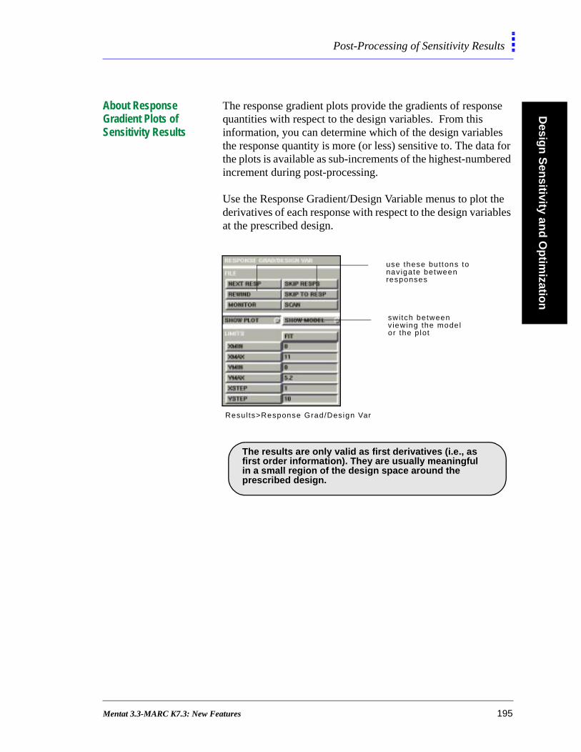
Desig
n S
ensitivity an
d O
ptim
ization
Post-Processing of Sensitivity Results
About Response Gradient Plots of Sensitivity Results
The response gradient plots provide the gradients of response quantities with respect to the design variables. From this information, you can determine which of the design variables the response quantity is more (or less) sensitive to. The data for the plots is available as sub-increments of the highest-numbered increment during post-processing.
Use the Response Gradient/Design Variable menus to plot the derivatives of each response with respect to the design variables at the prescribed design.
Resul ts>Response Grad/Design Var
use these buttons to nav igate between responses
switch betweenviewing the modelor the p lot
.
The results are only valid as first derivatives (i.e., as first order information). They are usually meaningful
prescribed design.in a small region of the design space around the
Mentat 3.3-MARC K7.3: New Features 195
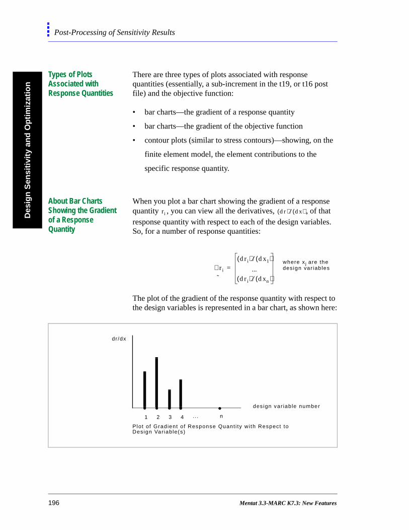
Des
ign
Sen
siti
vity
an
d O
pti
miz
atio
nPost-Processing of Sensitivity Results
e
e es.
t to here:
Types of Plots Associated with Response Quantities
There are three types of plots associated with response quantities (essentially, a sub-increment in the t19, or t16 post file) and the objective function:
• bar charts—the gradient of a response quantity
• bar charts—the gradient of the objective function
• contour plots (similar to stress contours)—showing, on th
finite element model, the element contributions to the
specific response quantity.
About Bar Charts Showing the Gradient of a Response Quantity
When you plot a bar chart showing the gradient of a responsquantity , you can view all the derivatives, , of thatresponse quantity with respect to each of the design variablSo, for a number of response quantities:
The plot of the gradient of the response quantity with respecthe design variables is represented in a bar chart, as shown
ri dr( ) dx( )⁄
∇ri
˜
dri( ) dx1( )⁄...
dri( ) dxn( )⁄
=where x j are thedesign var iab les
1 2 3 4 .. . n
design var iab le number
dr /dx
Plot of Gradient o f Response Quant i ty with Respect toDesign Variable(s)
196 Mentat 3.3-MARC K7.3: New Features
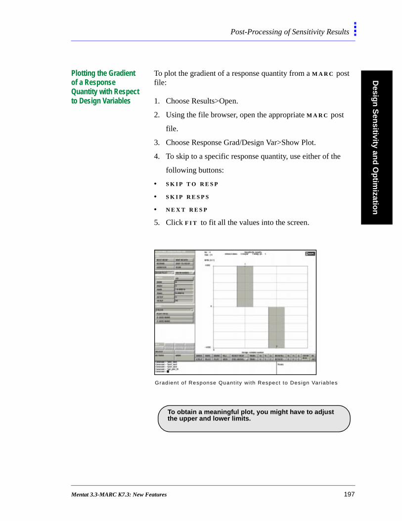
Desig
n S
ensitivity an
d O
ptim
ization
Post-Processing of Sensitivity Results
Plotting the Gradient of a Response Quantity with Respect to Design Variables
To plot the gradient of a response quantity from a M A R C post file:
1. Choose Results>Open.
2. Using the file browser, open the appropriate M A R C post
file.
3. Choose Response Grad/Design Var>Show Plot.
4. To skip to a specific response quantity, use either of the
following buttons:
• S K I P T O R E S P
• S K I P R E S P S
• N E X T R E S P
5. Click F I T to fit all the values into the screen.
Gradient o f Response Quant i ty wi th Respect to Design Var iables
. To obtain a meaningful plot, you might have to adjust
the upper and lower limits.
Mentat 3.3-MARC K7.3: New Features 197
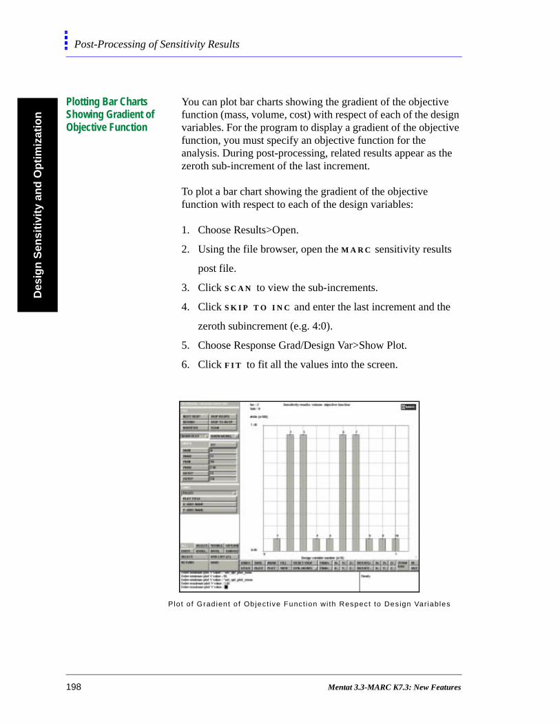
Des
ign
Sen
siti
vity
an
d O
pti
miz
atio
nPost-Processing of Sensitivity Results
Plotting Bar Charts Showing Gradient of Objective Function
You can plot bar charts showing the gradient of the objective function (mass, volume, cost) with respect of each of the design variables. For the program to display a gradient of the objective function, you must specify an objective function for the analysis. During post-processing, related results appear as the zeroth sub-increment of the last increment.
To plot a bar chart showing the gradient of the objective function with respect to each of the design variables:
1. Choose Results>Open.
2. Using the file browser, open the M A R C sensitivity results
post file.
3. Click S C A N to view the sub-increments.
4. Click S K I P T O I N C and enter the last increment and the
zeroth subincrement (e.g. 4:0).
5. Choose Response Grad/Design Var>Show Plot.
6. Click F I T to fit all the values into the screen.
Plot o f Gradient o f Object ive Funct ion wi th Respect to Design Variables
198 Mentat 3.3-MARC K7.3: New Features
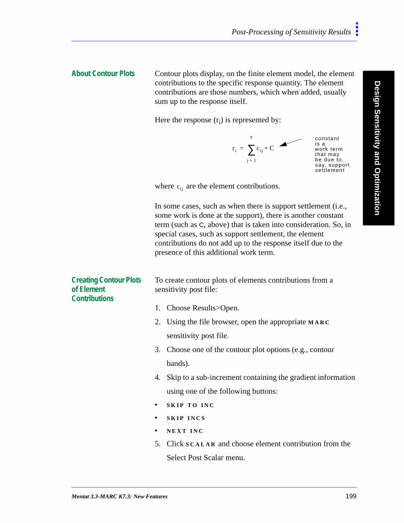
Desig
n S
ensitivity an
d O
ptim
ization
Post-Processing of Sensitivity Results
About Contour Plots Contour plots display, on the finite element model, the element contributions to the specific response quantity. The element contributions are those numbers, which when added, usually sum up to the response itself.
Here the response (ri) is represented by:
where are the element contributions.
In some cases, such as when there is support settlement (i.e., some work is done at the support), there is another constant term (such as C, above) that is taken into consideration. So, in special cases, such as support settlement, the element contributions do not add up to the response itself due to the presence of this additional work term.
Creating Contour Plots of Element Contributions
To create contour plots of elements contributions from a sensitivity post file:
1. Choose Results>Open.
2. Using the file browser, open the appropriate M A R C
sensitivity post file.
3. Choose one of the contour plot options (e.g., contour
bands).
4. Skip to a sub-increment containing the gradient information
using one of the following buttons:
• S K I P T O I N C
• S K I P I N C S
• N E X T I N C
5. Click S C A L A R and choose element contribution from the
Select Post Scalar menu.
ri cij
j 1=
n
∑ C+=
constant
work termis a
that may be due to ,say, suppor tset t lement
cij
Mentat 3.3-MARC K7.3: New Features 199

Des
ign
Sen
siti
vity
an
d O
pti
miz
atio
nPost-Processing of Sensitivity Results
6. Click R E S P O N S E G R A D / D E S I G N V A R .
7. Click S H O W M O D E L .
.
Contour P lot o f E lement Contr ibut ions f rom a Sensi t ivi ty Analys is
200 Mentat 3.3-MARC K7.3: New Features

Desig
n S
ensitivity an
d O
ptim
ization
Post-Processing of Optimization Results
o
en r ou ly, if
s ing
Post-Processing of Optimization Results
About Plotting of Optimization Results
You can create the following plots for optimization results in M E N T A T :
• history plots—the change in a response quantity or
objective function over the optimization cycles.
• bar chart—the values of the design variables at a cycle.
About History Plots of Optimization Results
History plots of optimization results show the change in the objective function, or a design variable, with the optimizationcycles. In the post file, the optimization cycles occur as sub-increments of the zeroth increment. The history plots are alspaired with information on whether each point on the plot represents a feasible (F), or an infeasible (I) design.
A design is considered feasible when it satisfies all of the givconstraints. An infeasible design is one which violates one omore of the constraints. If the violation is reasonably small, ycan decide whether the design is acceptable or not. Generalthe violation is less than the absolute, normalized value,
, the design is considered feasible.
The program traces history plots over the optimization cycle(sub-increments), with each integer x-axis value correspondto a sub-increment.
1 10 4–×
1 2 3 4 .. . M0
cycles
object ivefunct ion
F
F
IF
I
F
cycles s tar t a t 0 andstop at M
History of Object ive Funct ion Values over Opt im izat ion Cycles
Mentat 3.3-MARC K7.3: New Features 201

Des
ign
Sen
siti
vity
an
d O
pti
miz
atio
nPost-Processing of Optimization Results
Creating History Plots of Objective Function Values
To create a history plot of objective function values over optimization cycles:
1. Choose Results>Open.
2. Using the file browser, open the appropriate optimization
post file.
3. Click S C A N to view the increments.
4. Choose History Plot>Collect Data and enter the following
information:
• first increment
• last increment
• step size
5. Choose Nodes/Variables>Add Nodeless
6. From the list of design variables, choose:
• the plot variable for the X-axis (optimization cycles)
• the plot variable for the Y-axis (objective function)
7. Click F I T to fit all the values into the screen.
History Plot o f Object ive Funct ion with Respect toOpt imizat ion Cycles
202 Mentat 3.3-MARC K7.3: New Features

Desig
n S
ensitivity an
d O
ptim
ization
Post-Processing of Optimization Results
About History Plots of Design Variable Values over Optimization Cycles
You can plot the change in the values of design variables over the optimization cycles using the same commands as in creating a plot for objective function.
de
sig
n v
ari
ab
le v
alu
es
de
sig
n v
ari
ab
le v
alu
es
de
sig
n v
ari
ab
le v
alu
es
X1 X2 Xn
0 1 2 .. . Mcycles
0 1 2 .. . Mcycles
0 1 2 .. . Mcycles
Plot o f Design Var iab le Values (Xj) over Opt imizat ion Cycles
Mentat 3.3-MARC K7.3: New Features 203

Des
ign
Sen
siti
vity
an
d O
pti
miz
atio
nPost-Processing of Optimization Results
Creating History Plots of Design Variable Values
To create history plots of design variable values over optimization cycles:
1. Choose Results>Open.
2. Using the file browser, open the optimization results file.
3. Click C O L L E C T D A T A and enter the following
information:
• first increment
• last increment
• step size
4. Choose Nodes/Variables>Add Nodeless
5. From the list of design variables, choose:
• the plot variable for the X-axis (optimization cycles)
• a design variable for the Y-axis
6. Click F I T to fit all the values into the screen.
History P lot o f Design Variable Values wi th Respect toOpt imizat ion Cycles
204 Mentat 3.3-MARC K7.3: New Features

Desig
n S
ensitivity an
d O
ptim
ization
Post-Processing of Optimization Results
Creating Bar Charts of Design Variables Values
To create bar charts of design variable values at the end of a cycle:
1. Choose Results>Open.
2. Using the file browser, open the appropriate optimization
file.
3. Choose Response Grad/Design Var>Show Plot.
4. To skip to a specific sub-increment, use either of the
following buttons:
• S K I P T O I N C
• S K I P I N C S
• N E X T I N C
5. Click F I T to fit all the values into the screen.
Design Var iab le Values at the End of a Cycle
Mentat 3.3-MARC K7.3: New Features 205
Des
ign
Sen
siti
vity
an
d O
pti
miz
atio
nPost-Processing of Optimization Results
Additional Information Use the following table to find more information:
For... refer to Chapter/s...
in...
definitions of individual buttons in the Results menus
13: Results Mentat 3.1 Command Reference
background information and theoretical discussion
5: Structural Procedure Library
Vol. A
206 Mentat 3.3-MARC K7.3: New Features
8• Element Technology
New Shell Elements
About the New Shell Elements 209About Element 138 209About Element 139 210About Element 140 210Associating Elements with a 3-D Membrane/Shell 211
New Rebar Elements
About Rebar Elements 212Types of Rebar Elements 212Generating and Identifying Rebar Elements 213Specifying Rebar Material Properties 214Associating Double Elements with Nodes 215
Mentat 3.3-MARC K7.3: New Features 207

• Element Technology
Mentat 3.3-MARC K7.3: New Features
Elem
ent Tech
no
log
yNew Shell Elements
e a
r
New Shell Elements
About the New Shell Elements
The following element types are now available in M A R C :
• 138
• 139
• 140
Like all other M A R C shell-elements, these three elements usnumerical integration through the thickness. The default number is 11.
You can modify the number of layers per shell by using eitheof the following options:
• composites
• job parameters
About Element 138 Element 138 is a four-node, thin-shell element based on theDiscrete Kirchoff theory.
These are some of the salient features of Element 138:
• triangular element; works very well with the triangular
mesh generators that are available in Mentat or in other
CAD programs
• ease of use
• six degrees of freedom per node
• requires no tying
• applicable to all the material models in M A R C
Mentat 3.3-MARC K7.3: New Features 209

Ele
men
t Te
chn
olo
gy
New Shell Elements
ed
nt
ty
About Element 139 Element 139 is a four-node, thin-shell element based on the Discrete Kirchoff shell theory.
These are some of the salient features of Element 139:
• similar to Element 75, but uses thin-shell theory as oppos
to thick-shell theory
• suitable for thin-shell structures
• applicable to all the material models that are in M A R C
• six degrees of freedom per node
• four integration points per layer
• about five times faster than Element 75 during the eleme
assembly phase
About Element 140 Element 140 is a four-node, thick-shell element similar to Element 75 but uses a single integration point per element.
These are some of the salient features of Element 140:
• six degrees of freedom
• uses hourglass stiffness matrix to insure that it is a stable
element
• cheaper to use but not as accurate in the case of plastici
analysis
• about two-and-a-half times faster than Element 75 during
the element assembly phase
210 Mentat 3.3-MARC K7.3: New Features

Elem
ent Tech
no
log
yNew Shell Elements
Associating Elements with a 3-D Membrane/Shell
Before you associate elements types with your 3-D Membrane/Shell element, you should create your mesh using three-node or four-node elements.
To list elements with a 3-D Membrane/Shell element:
1. Choose Jobs>Element Types.
2. Click 3 - D M E M B R A N E / S H E L L .
3. Choose the elements to associate.
4. Click O K .
5. Select elements.
Additional Information Use the following table to find more information:
use for 4-nodeelements
use for 3-nodeelements
For... refer to Chapter/s...
in...
notes on shell orientation, layers
1:MARC System Vol. A
description of the elements
3: Element Library ‘Vol. B
Mentat 3.3-MARC K7.3: New Features 211

Ele
men
t Te
chn
olo
gy
New Rebar Elements
ing
f a ve
New Rebar Elements
About Rebar Elements Rebar elements are, essentially, hollow elements with uniaxial stiffness. You can place single strain members in rebar elements.
Use rebar elements to represent stiffness elements that are present in a single direction through the matrix material. Although the rebar layer concept was originally applied to steel rebars in concrete civil engineering applications, you can use rebar elements in composite materials—composites containsmall filaments (e.g., tires in which there are belts running through the rubber material).
The orientation of single strain members in different layers orebar element may be different. Each rebar element may haup to five rebar layers oriented in a particular direction. Eachone of the layers has a different material behavior.
Types of Rebar Elements
Here are the types of rebar elements available in M A R C /M E N T A T :
• plane-strain rebar elements (four-node and eight-node)
• generalized plane-strain elements (eight-node)
different or ientat ionsof s ing le s tra inmembers/ layers of a rebar e lementa
212 Mentat 3.3-MARC K7.3: New Features
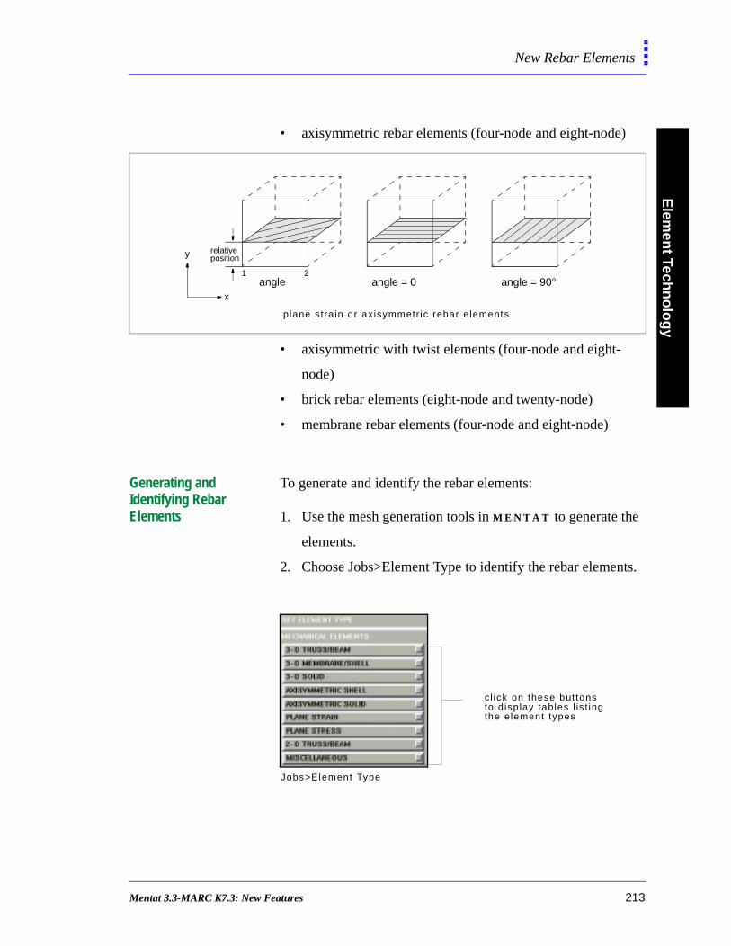
Elem
ent Tech
no
log
yNew Rebar Elements
ts.
• axisymmetric rebar elements (four-node and eight-node)
• axisymmetric with twist elements (four-node and eight-
node)
• brick rebar elements (eight-node and twenty-node)
• membrane rebar elements (four-node and eight-node)
Generating and Identifying Rebar Elements
To generate and identify the rebar elements:
1. Use the mesh generation tools in M E N T A T to generate the
elements.
2. Choose Jobs>Element Type to identify the rebar elemen
angle = 90°angle = 0angle1 2
relativepositiony
x
plane stra in or ax isymmetr ic rebar e lements
c l ick on these but tonsto d isp lay tab les l is t ingthe element types
Jobs>Element Type
Mentat 3.3-MARC K7.3: New Features 213

Ele
men
t Te
chn
olo
gy
New Rebar Elements
Specifying Rebar Material Properties
Use the Materials Properties menus to specify the properties of rebar elements including the direction of uniaxial behavior.
To specify rebar material properties:
1. Choose Material Properties>New Rebar-Define.
2. Specify the orientation of uniaxial behavior.
3. Choose the number of layers for the rebar element.
4. Specify the following properties for one or more layers:
• relative position of this rebar layer in the element (this
number is between 0.0 and 1.0).
• cross-sectional area of the rebar.
speci fy rebarmateria lproper t ies forup to f ive layers
Mater ial Proper t ies>New Rebar>Def ine
214 Mentat 3.3-MARC K7.3: New Features
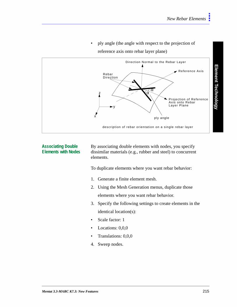
Elem
ent Tech
no
log
yNew Rebar Elements
• ply angle (the angle with respect to the projection of
reference axis onto rebar layer plane)
Associating Double Elements with Nodes
By associating double elements with nodes, you specify dissimilar materials (e.g., rubber and steel) to concurrent elements.
To duplicate elements where you want rebar behavior:
1. Generate a finite element mesh.
2. Using the Mesh Generation menus, duplicate those
elements where you want rebar behavior.
3. Specify the following settings to create elements in the
identical location(s):
• Scale factor: 1
• Locations: 0,0,0
• Translations: 0,0,0
4. Sweep nodes.
Rebar
Direct ion Normal to the Rebar Layer
Reference Axis
Pro ject ion of ReferenceAxis onto Rebar
z
y
x
-αα
Layer Plane
Direct ion
ply angle
descr ip t ion of rebar or ientat ion on a s ingle rebar layer
Mentat 3.3-MARC K7.3: New Features 215
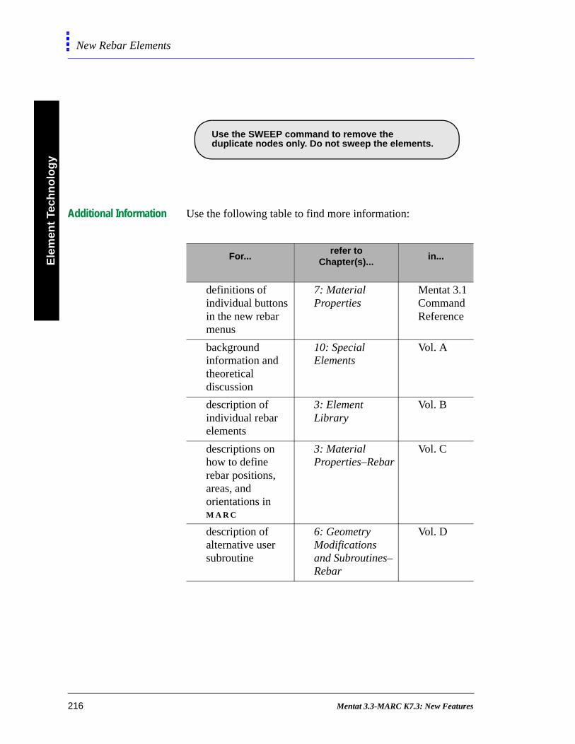
Ele
men
t Te
chn
olo
gy
New Rebar Elements
Additional Information Use the following table to find more information:
Use the SWEEP command to remove theduplicate nodes only. Do not sweep the elements.
For...refer to
Chapter(s)...in...
definitions of individual buttons in the new rebar menus
7: Material Properties
Mentat 3.1 Command Reference
background information and theoretical discussion
10: Special Elements
Vol. A
description of individual rebar elements
3: Element Library
Vol. B
descriptions on how to define rebar positions, areas, and orientations in M A R C
3: Material Properties–Rebar
Vol. C
description of alternative user subroutine
6: Geometry Modifications and Subroutines– Rebar
Vol. D
216 Mentat 3.3-MARC K7.3: New Features
9• Fluid Mechanics
Fluid Analysis
About Fluid Analysis Options 222About the Solver Option for Fluid Analysis 225
Boundary Conditions for Fluid Analysis
About Boundary Conditions for Fluid Analysis 226About Centrifugal Loads 231
Initial Conditions for Fluid Analysis
About Velocity as Initial Condition Type 233Coupled Analysis Considerations 233
Material Properties for Fluid Analysis
About Fluid Properties and Viscosity Models 235Mass Density and Volumetric Expansion 237
Loadcases for Fluid Analysis
Applying the Fluid Steady State Parameters 239About Iterative Procedures in Solution Control 241
Mentat 3.3-MARC K7.3: New Features 217

Mentat 3.3-MARC K7.3: New Features

Flu
id M
echan
ics
Mentat 3.3-MARC K7.3: New Features 219

Flu
id M
ech
anic
s
• Fluid Mechanics
220 Mentat 3.3-MARC K7.3: New Features
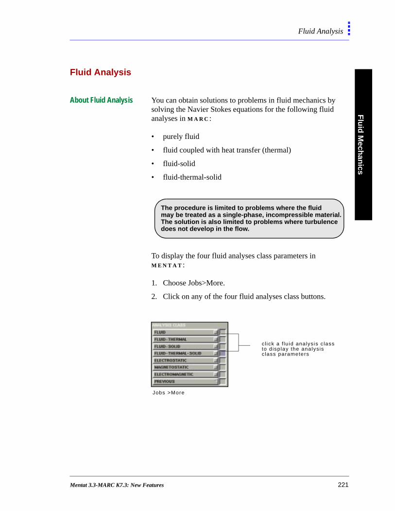
Flu
id M
echan
icsFluid Analysis
Fluid Analysis
About Fluid Analysis You can obtain solutions to problems in fluid mechanics by solving the Navier Stokes equations for the following fluid analyses in M A R C :
• purely fluid
• fluid coupled with heat transfer (thermal)
• fluid-solid
• fluid-thermal-solid
To display the four fluid analyses class parameters in M E N T A T :
1. Choose Jobs>More.
2. Click on any of the four fluid analyses class buttons.
.
The procedure is limited to problems where the fluidmay be treated as a single-phase, incompressible material.The solution is also limited to problems where turbulencedoes not develop in the flow.
cl ick a f lu id analys is c lassto d isp lay the analys isc lass parameters
Jobs >More
Mentat 3.3-MARC K7.3: New Features 221
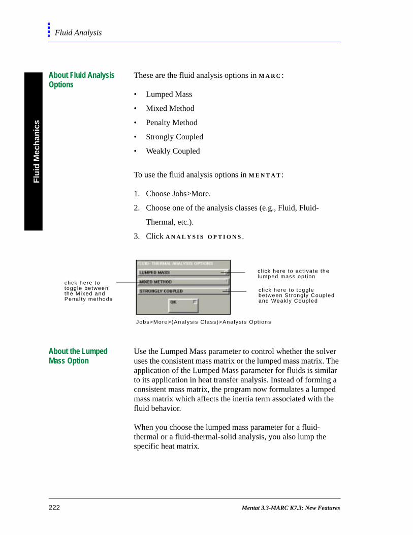
Flu
id M
ech
anic
sFluid Analysis
ver The ar a ed e
About Fluid Analysis Options
These are the fluid analysis options in M A R C :
• Lumped Mass
• Mixed Method
• Penalty Method
• Strongly Coupled
• Weakly Coupled
To use the fluid analysis options in M E N T A T :
1. Choose Jobs>More.
2. Choose one of the analysis classes (e.g., Fluid, Fluid-
Thermal, etc.).
3. Click A N A L Y S I S O P T I O N S .
About the Lumped Mass Option
Use the Lumped Mass parameter to control whether the soluses the consistent mass matrix or the lumped mass matrix.application of the Lumped Mass parameter for fluids is similto its application in heat transfer analysis. Instead of formingconsistent mass matrix, the program now formulates a lumpmass matrix which affects the inertia term associated with thfluid behavior.
When you choose the lumped mass parameter for a fluid-thermal or a fluid-thermal-solid analysis, you also lump the specific heat matrix.
c l ick here to togglebetween Strongly Coupledand Weakly Coupled
cl ick here to act ivate thelumped mass opt ion
cl ick here totoggle betweenthe Mixed andPenal ty methods
Jobs>More>(Analys is Class)>Analys is Opt ions
222 Mentat 3.3-MARC K7.3: New Features

Flu
id M
echan
icsFluid Analysis
So
e of ty
s
l
oo is ll.
About Mixed and Penalty Method Procedures
You can toggle the buttons between the Mixed Method and Penalty Method parameters in M E N T A T to select a procedure that ensures that the fluid is computationally treated as incompressible.
When you use the Mixed Method, there is an additional degree of freedom–a pressure degree of freedom–at all the nodes. the degrees of freedom involve the velocities and pressure.
When you specify the Penalty Method parameter, the degrefreedom involves the velocities only and an additional penalfunction. The penalty function is a scalar function and you specify the value of the function in the Numerical Preferenceoption.
The Mixed Method procedure is more accurate but requiresmore computational resources because there is an additionadegree of freedom for every node. This makes the stiffness matrix larger and the solution of the equation more computationally expensive.
In the Penalty Method, if the value of the Penalty function is tlarge, it might affect the accuracy of the solution process. This reflected in a singularity ratio that might be extremely smaIf the value of the penalty function is too small, the fluid will not satisfy the incompressibility requirement.
Mentat 3.3-MARC K7.3: New Features 223

Flu
id M
ech
anic
sFluid Analysis
ly-t ry
Specifying a Value for Penalty Function
To specify the value of the Penalty function for fluid analysis:
1. Click J O B S .
2. Choose a fluid analysis class (e.g., Fluid, Fluid-Thermal,
etc.)
3. Choose Job Parameters>Numerical Preferences.
4. Click F L U I D I N C O M P R E S S I B I L I T Y P E N A L T Y and
specify a value.
About Strongly-Coupled and Weakly-Coupled Parameters
The Strongly-Coupled parameters apply to fluid-thermal and fluid-thermal-solid analyses only. Using these parameters, you can simultaneously solve the velocity of the fluid and the temperature of the fluid. This simultaneous solution also results in an additional degree of freedom per node.
Use the Weakly-Coupled parameters to solve the following in sequence:
• velocity
• temperature of the fluid
The Weakly-Coupled procedure is also known as the “Staggered” procedure.
The Strongly-Coupled procedure is better suited for thermaldriven fluid problems. The Weakly-Coupled procedure mighrun into stability problems when the temperature changes ve
Jobs>(Analys is Class)>Job Parameters>Numerica l Preferences
224 Mentat 3.3-MARC K7.3: New Features
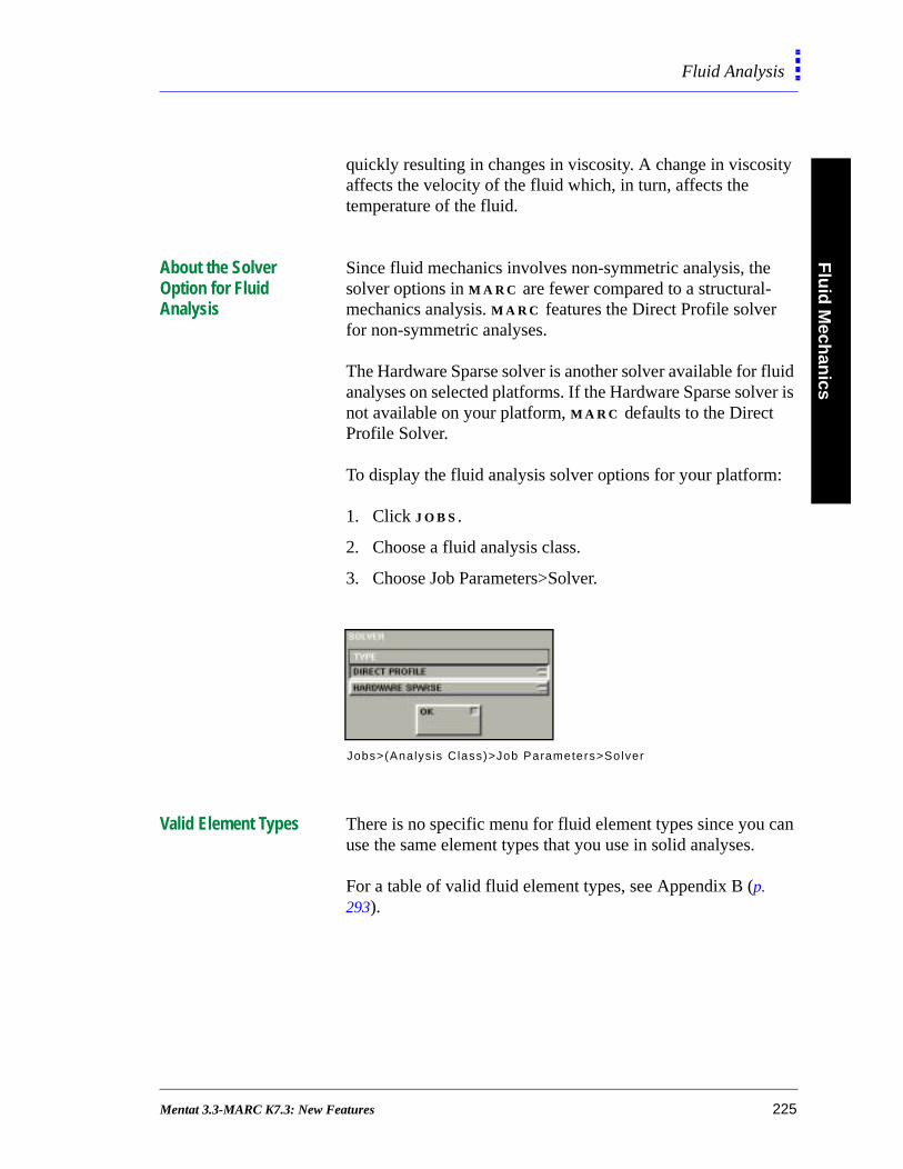
Flu
id M
echan
icsFluid Analysis
quickly resulting in changes in viscosity. A change in viscosity affects the velocity of the fluid which, in turn, affects the temperature of the fluid.
About the Solver Option for Fluid Analysis
Since fluid mechanics involves non-symmetric analysis, the solver options in M A R C are fewer compared to a structural-mechanics analysis. M A R C features the Direct Profile solver for non-symmetric analyses.
The Hardware Sparse solver is another solver available for fluid analyses on selected platforms. If the Hardware Sparse solver is not available on your platform, M A R C defaults to the Direct Profile Solver.
To display the fluid analysis solver options for your platform:
1. Click J O B S .
2. Choose a fluid analysis class.
3. Choose Job Parameters>Solver.
Valid Element Types There is no specific menu for fluid element types since you can use the same element types that you use in solid analyses.
For a table of valid fluid element types, see Appendix B (p. 293).
Jobs>(Analys is Class)>Job Parameters>Solver
Mentat 3.3-MARC K7.3: New Features 225
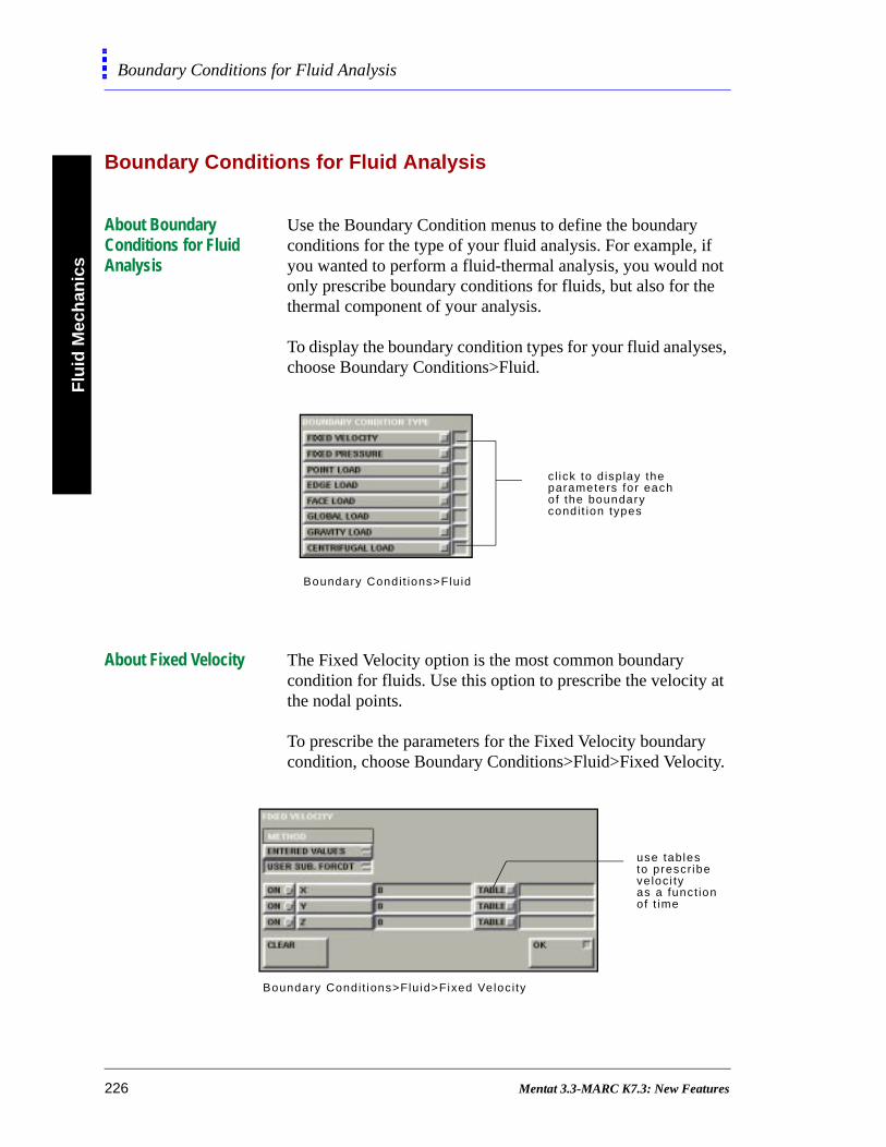
Flu
id M
ech
anic
sBoundary Conditions for Fluid Analysis
Boundary Conditions for Fluid Analysis
About Boundary Conditions for Fluid Analysis
Use the Boundary Condition menus to define the boundary conditions for the type of your fluid analysis. For example, if you wanted to perform a fluid-thermal analysis, you would not only prescribe boundary conditions for fluids, but also for the thermal component of your analysis.
To display the boundary condition types for your fluid analyses, choose Boundary Conditions>Fluid.
About Fixed Velocity The Fixed Velocity option is the most common boundary condition for fluids. Use this option to prescribe the velocity at the nodal points.
To prescribe the parameters for the Fixed Velocity boundary condition, choose Boundary Conditions>Fluid>Fixed Velocity.
cl ick to d isp lay the parameters for eachof the boundarycondit ion types
Boundary Condit ions>Flu id
use tablesto prescribeveloc i tyas a funct ionof t ime
Boundary Condit ions>Flu id>Fixed Veloc i ty
226 Mentat 3.3-MARC K7.3: New Features

Flu
id M
echan
icsBoundary Conditions for Fluid Analysis
To set the parameters, refer to the following table:
For transient analyses, you can use the user subroutine FORCDT (See Vol. D: User Subroutines–FORCDT) or tables to specify the time-dependent velocity.
If the analysis is for a ... then...
steady state fluid problem
prescribe the final velocities at the nodal points.
transient state fluids you can enter a table prescribing how the velocities change with time.
2-D problem prescribe the X and Y velocities.
3-D problem prescribe the X, Y, and Z velocities.
. To prevent the incidence of a single set of equations
in a fluid analysis, you should apply some boundarycondition to the fluid.
Mentat 3.3-MARC K7.3: New Features 227
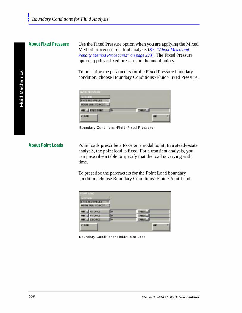
Flu
id M
ech
anic
sBoundary Conditions for Fluid Analysis
About Fixed Pressure Use the Fixed Pressure option when you are applying the Mixed Method procedure for fluid analysis (See “About Mixed and Penalty Method Procedures” on page 223). The Fixed Pressure option applies a fixed pressure on the nodal points.
To prescribe the parameters for the Fixed Pressure boundary condition, choose Boundary Conditions>Fluid>Fixed Pressure.
About Point Loads Point loads prescribe a force on a nodal point. In a steady-state analysis, the point load is fixed. For a transient analysis, you can prescribe a table to specify that the load is varying with time.
To prescribe the parameters for the Point Load boundary condition, choose Boundary Conditions>Fluid>Point Load.
Boundary Condit ions>Fluid>Fixed Pressure
Boundary Condi t ions>Flu id>Point Load
228 Mentat 3.3-MARC K7.3: New Features
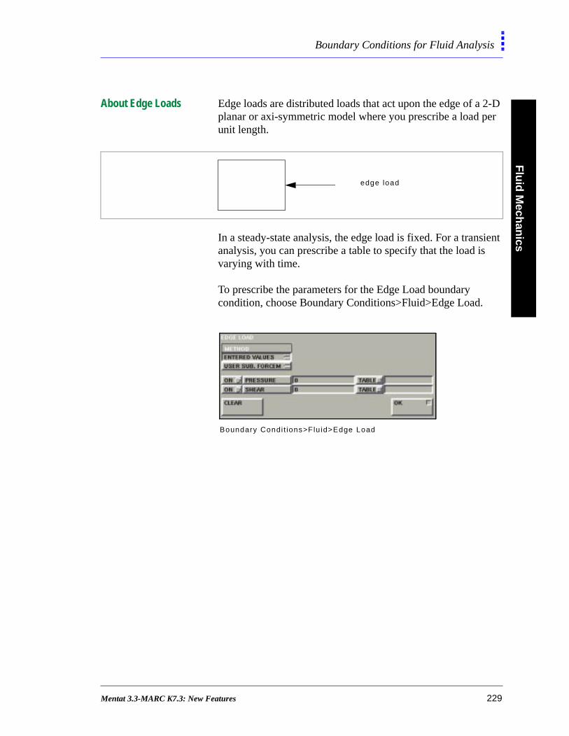
Flu
id M
echan
icsBoundary Conditions for Fluid Analysis
About Edge Loads Edge loads are distributed loads that act upon the edge of a 2-D planar or axi-symmetric model where you prescribe a load per unit length.
In a steady-state analysis, the edge load is fixed. For a transient analysis, you can prescribe a table to specify that the load is varying with time.
To prescribe the parameters for the Edge Load boundary condition, choose Boundary Conditions>Fluid>Edge Load.
edge load
Boundary Condi t ions>Flu id>Edge Load
Mentat 3.3-MARC K7.3: New Features 229

Flu
id M
ech
anic
sBoundary Conditions for Fluid Analysis
About Face Loads Face loads are loads acting upon a face for a 3-D problem. A positive load implies that the load is directed into the element.
To prescribe the parameters for the Face Load boundary condition, choose Boundary Conditions>Fluid>Face Load.
About Global Loads Global loads are loads per unit volume.
To prescribe the parameters for the Global Load boundary condition, choose Boundary Conditions>Fluid>Global Load.
face load
Boundary Condi t ions>Flu id>Face Load
Boundary Condit ions>Fluid>Global Load
230 Mentat 3.3-MARC K7.3: New Features
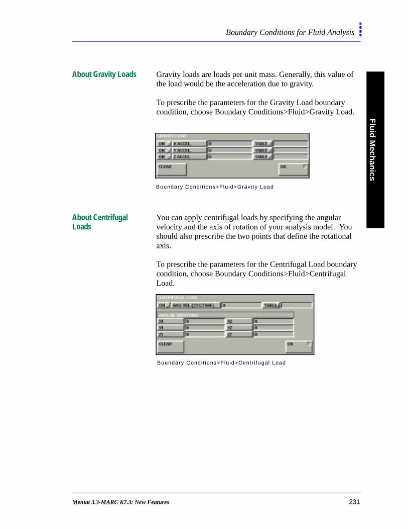
Flu
id M
echan
icsBoundary Conditions for Fluid Analysis
About Gravity Loads Gravity loads are loads per unit mass. Generally, this value of the load would be the acceleration due to gravity.
To prescribe the parameters for the Gravity Load boundary condition, choose Boundary Conditions>Fluid>Gravity Load.
About Centrifugal Loads
You can apply centrifugal loads by specifying the angular velocity and the axis of rotation of your analysis model. You should also prescribe the two points that define the rotational axis.
To prescribe the parameters for the Centrifugal Load boundary condition, choose Boundary Conditions>Fluid>Centrifugal Load.
Boundary Condit ions>Fluid>Gravi ty Load
Boundary Condit ions>Fluid>Cent r i fugal Load
Mentat 3.3-MARC K7.3: New Features 231

Flu
id M
ech
anic
sInitial Conditions for Fluid Analysis
s
re .
Initial Conditions for Fluid Analysis
About Types of Initial Conditions
There are three types of initial conditions that you can specify in a fluid analysis:
• Mechanical
• Thermal
• Fluid
To display the types of initial conditions in M E N T A T , choose Initial Conditions in Main Menu.
Depending on the type of analysis, you may require initial conditions for one or all of the types. For example, if it is a purely fluid analysis, you may need initial conditions for fluidonly.
If you perform a steady state analysis, the initial conditions anot as relevant as they would be in a transient state analysis
choose th is opt ionfor a pure ly f lu id analys is
Ini t ia l Condit ions
.
Picking good initial conditions (conditions that areclose to the final solution) can result in improved convergence in the numerical analysis. However, theywill not influence the final results.
232 Mentat 3.3-MARC K7.3: New Features
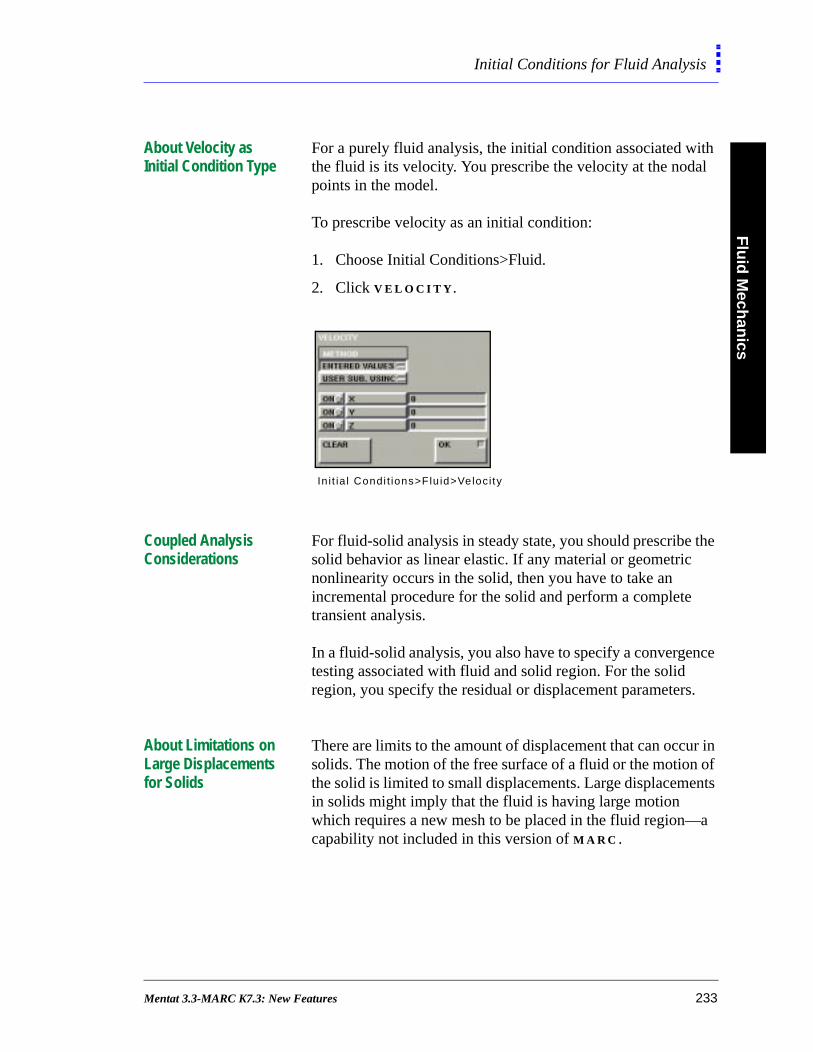
Flu
id M
echan
icsInitial Conditions for Fluid Analysis
a
About Velocity as Initial Condition Type
For a purely fluid analysis, the initial condition associated with the fluid is its velocity. You prescribe the velocity at the nodal points in the model.
To prescribe velocity as an initial condition:
1. Choose Initial Conditions>Fluid.
2. Click V E L O C I T Y.
Coupled Analysis Considerations
For fluid-solid analysis in steady state, you should prescribe the solid behavior as linear elastic. If any material or geometric nonlinearity occurs in the solid, then you have to take an incremental procedure for the solid and perform a complete transient analysis.
In a fluid-solid analysis, you also have to specify a convergence testing associated with fluid and solid region. For the solid region, you specify the residual or displacement parameters.
About Limitations on Large Displacements for Solids
There are limits to the amount of displacement that can occur in solids. The motion of the free surface of a fluid or the motion of the solid is limited to small displacements. Large displacements in solids might imply that the fluid is having large motion which requires a new mesh to be placed in the fluid region—capability not included in this version of M A R C .
In i t ia l Condi t ions>Flu id>Veloci ty
Mentat 3.3-MARC K7.3: New Features 233
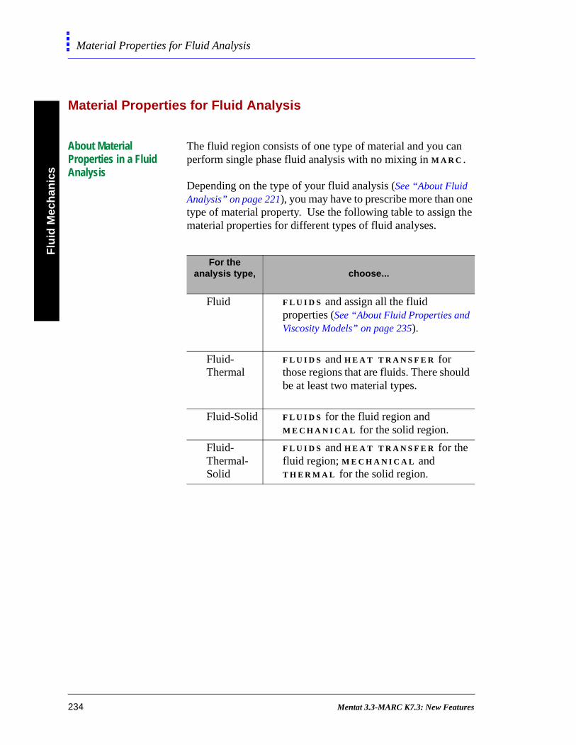
Flu
id M
ech
anic
sMaterial Properties for Fluid Analysis
Material Properties for Fluid Analysis
About Material Properties in a Fluid Analysis
The fluid region consists of one type of material and you can perform single phase fluid analysis with no mixing in M A R C .
Depending on the type of your fluid analysis (See “About Fluid Analysis” on page 221), you may have to prescribe more than one type of material property. Use the following table to assign the material properties for different types of fluid analyses.
For the analysis type, choose...
Fluid F L U I D S and assign all the fluid properties (See “About Fluid Properties and Viscosity Models” on page 235).
Fluid-Thermal
F L U I D S and H E A T T R A N S F E R for those regions that are fluids. There should be at least two material types.
Fluid-Solid F L U I D S for the fluid region and M E C H A N I C A L for the solid region.
Fluid-Thermal-Solid
F L U I D S and H E A T T R A N S F E R for the fluid region; M E C H A N I C A L and T H E R M A L for the solid region.
234 Mentat 3.3-MARC K7.3: New Features
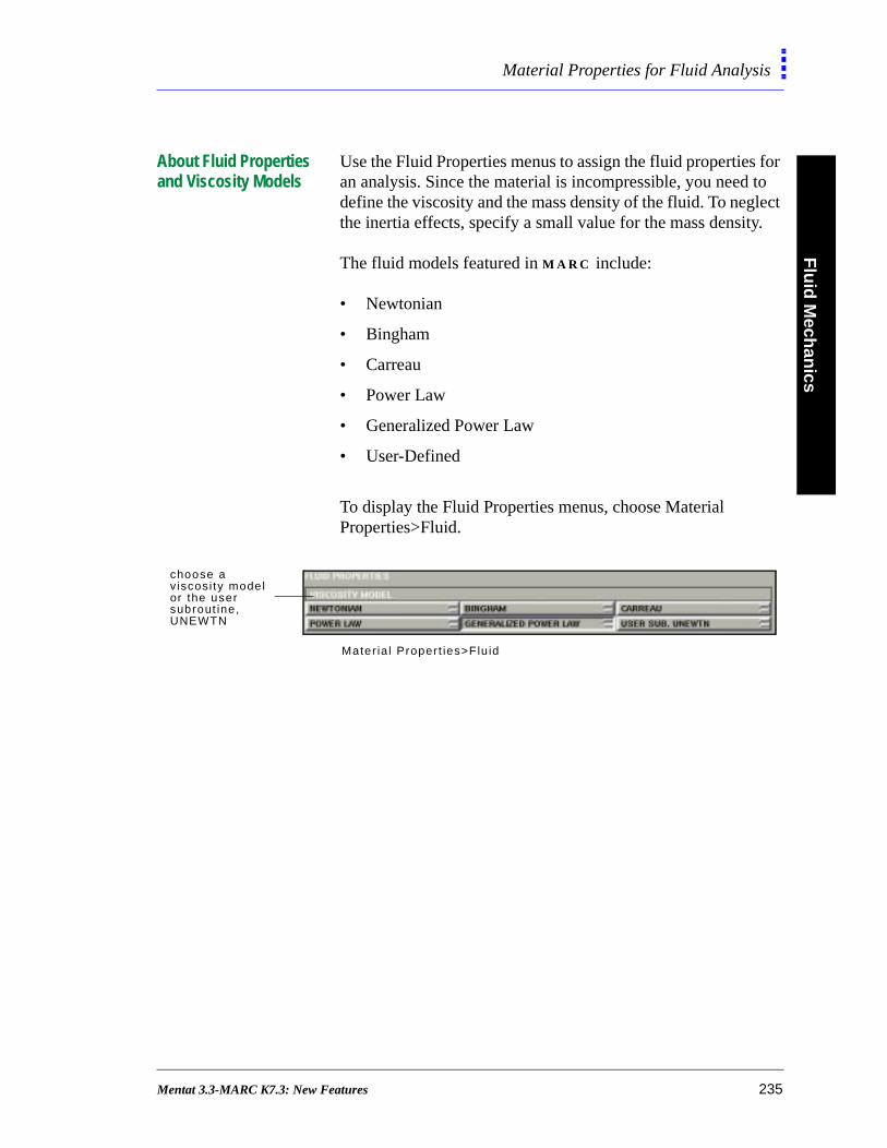
Flu
id M
echan
icsMaterial Properties for Fluid Analysis
About Fluid Properties and Viscosity Models
Use the Fluid Properties menus to assign the fluid properties for an analysis. Since the material is incompressible, you need to define the viscosity and the mass density of the fluid. To neglect the inertia effects, specify a small value for the mass density.
The fluid models featured in M A R C include:
• Newtonian
• Bingham
• Carreau
• Power Law
• Generalized Power Law
• User-Defined
To display the Fluid Properties menus, choose Material Properties>Fluid.
choose a v iscosi ty modelor the user subrout ine, UNEWTN
Mater ia l Proper t ies>Flu id
Mentat 3.3-MARC K7.3: New Features 235

Flu
id M
ech
anic
sMaterial Properties for Fluid Analysis
e
Use the following table to define the parameters for each of the viscosity models:
For... define...
Newtonian fluids
the viscosity or a table that represents the temperature effects on viscosity.
Bingham fluids
the viscosity and the following tables:
• temperature-dependent behavior• rate (strain rate) behavior
as given by the relation:
Carreau model fluids
The values of K, D, and n as given by threlation:
Power Law fluids
K, n, and D as given by the relation:
Generalized Power Law fluids
K, η, D, A1, A2, A3, A4 as given by the relation:
where
τij µ0dij gD 1– dij if τ g≥+=
dij 0= if τ g<
µ µ∞ µ0 µ∞–( ) 1 K2D2+( )n 1–( ) 2⁄
+=
τij µ0KDn 1– dij=
µ0K exp A1T A2T2+( )D0P D D0<
µ0K exp A1T A2T2+( )DP D D0≥µ =
P n 1– A3 D A4T+ln+=
236 Mentat 3.3-MARC K7.3: New Features
Flu
id M
echan
icsMaterial Properties for Fluid Analysis
Mass Density and Volumetric Expansion
You must enter the mass density for fluids and, if it is a fluid-thermal analysis, the volumetric expansion coefficient. When you enter a value for the volumetric expansion, the fluid is allowed to change its volume owing to a change in temperature based upon the temperature coefficient.
The M A R C models of fluids assume that the mass density is constant and thus exclude gases.
.
You can use the subroutine, UNEWTN, to define the viscosity at a particular spatial location. For more information, see Vol. D: UNEWTN: Input of Viscosityin Flow Analysis
Mentat 3.3-MARC K7.3: New Features 237

Flu
id M
ech
anic
sLoadcases for Fluid Analysis
re
Loadcases for Fluid Analysis
About Loadcases for Fluids
You can choose the following loadcase classes depending on the type of fluid analysis in M E N T A T :
• Fluid
• Fluid-Thermal
• Fluid-Solid
• Fluid-Thermal-Solid
For each of the above loadcase classes, you can specify thefollowing loadcase types:
• Steady State—you define the tolerance value to control
convergence and accuracy
• Transient—you define the tolerance value to control
convergence and accuracy, the time steps, and the total
loadcase time.
The parameters and menus for the Fluid loadcase classes asimilar to Heat Transfer parameters and menus (See Mentat Command Reference Manual, Chapter 11: Analysis-Loadcases).
To display the Loadcase Type menu:
1. Click L O A D C A S E in Main Menu.
2. Choose a loadcase class (e.g., Fluid, Fluid-Solid).
Loadcase>(Loadcase Class)
238 Mentat 3.3-MARC K7.3: New Features
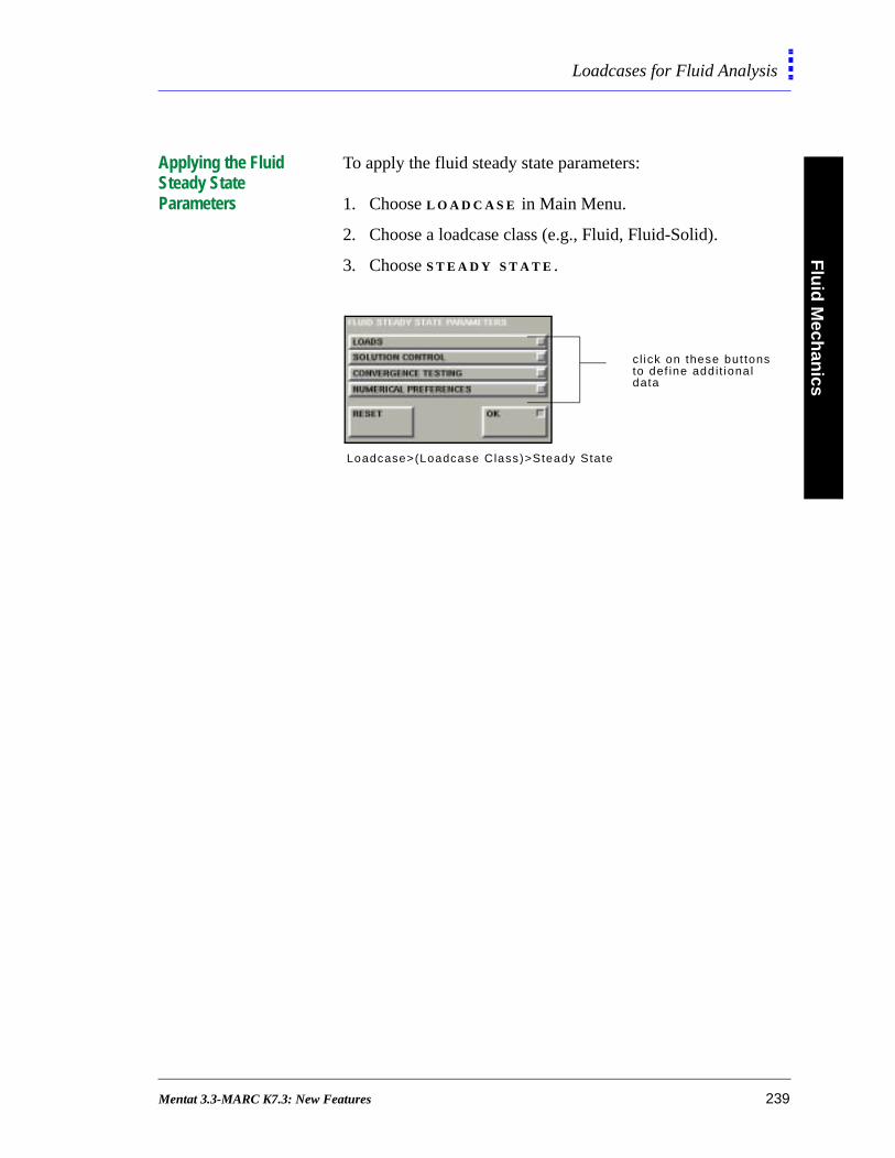
Flu
id M
echan
icsLoadcases for Fluid Analysis
Applying the Fluid Steady State Parameters
To apply the fluid steady state parameters:
1. Choose L O A D C A S E in Main Menu.
2. Choose a loadcase class (e.g., Fluid, Fluid-Solid).
3. Choose S T E A D Y S T A T E .
c l ick on these but tonsto def ine addit ionaldata
Loadcase>(Loadcase Class)>Steady State
Mentat 3.3-MARC K7.3: New Features 239

Flu
id M
ech
anic
sLoadcases for Fluid Analysis
Applying the Fluid Transient Parameters
To apply the transient parameters for a fluid analysis:
1. Choose L O A D C A S E in Main Menu.
2. Choose a loadcase class (e.g., Fluid, Fluid-Solid).
3. Choose T R A N S I E N T .
4. Click T O T A L L O A D C A S E T I M E and specify the total
loadcase time period.
5. Choose fixed or adaptive time steps.
Loadcase>(Loadcase Class)>Transient
.
Since fluid analyses is a highly nonlinear phenomenon, you might need to take small steps to achieve convergencefor a transient analysis.
240 Mentat 3.3-MARC K7.3: New Features
Flu
id M
echan
icsLoadcases for Fluid Analysis
he
or
ly-
About Iterative Procedures in Solution Control
You can apply either of the iterative procedures for solution control in M A R C :
• Full Newton-Raphson
At each iteration of the Newton-Raphson procedure, yousolve:
where Xi is the solution at the ith iteration, and Ri is the error in the solution or residual. Each iteration results in t
change δXi+1 in the solution.
• Direct Substitution
For the Direct Substitution procedure, you solve:
where the force remains for all iterations, and the operatmatrix is obtained from the last solution of X.
About Control Tolerances
When you perform a coupled analysis with either the StrongCoupled or Weakly-Coupled method you should specify twoseparate control tolerances for the:
• velocity
• temperature change in the fluid
O X( )δXi 1+ Ri=
Xi 1+ Xi δXi 1++=
O Xi( )Xi 1+ F=
. When the Full Newton-Raphson procedure converges,it converges faster. However, the Direct Substitutionprocedure is often numerically more stable.
Mentat 3.3-MARC K7.3: New Features 241
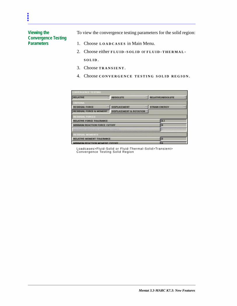
Viewing the Convergence Testing Parameters
To view the convergence testing parameters for the solid region:
1. Choose L O A D C A S E S in Main Menu.
2. Choose either F L U I D - S O L I D or F L U I D - T H E R M A L -
S O L I D .
3. Choose T R A N S I E N T .
4. Choose C O N V E R G E N C E T E S T I N G S O L I D R E G I O N .
Loadcases>Flu id-Sol id or Flu id-Thermal-Sol id>Transient>Convergence Test ing Sol id Region
Mentat 3.3-MARC K7.3: New Features
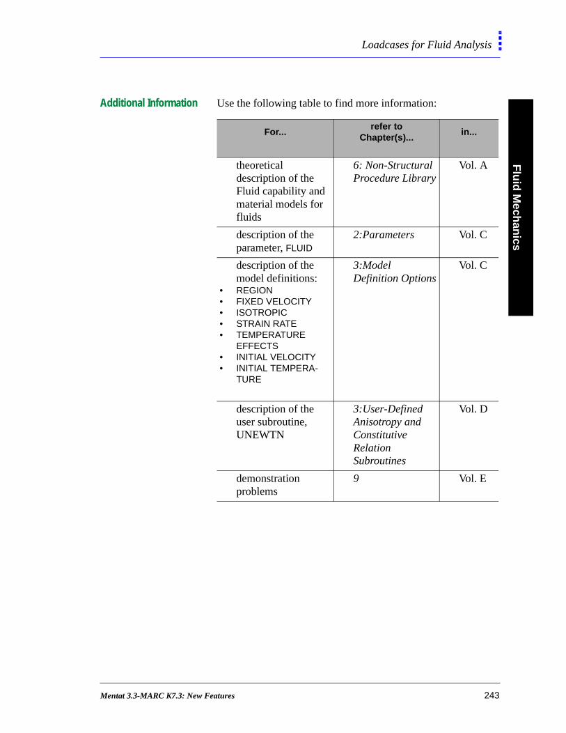
Flu
id M
echan
icsLoadcases for Fluid Analysis
Additional Information Use the following table to find more information:
For...refer to
Chapter(s)...in...
theoretical description of the Fluid capability and material models for fluids
6: Non-Structural Procedure Library
Vol. A
description of the parameter, FLUID
2:Parameters Vol. C
description of the model definitions:
• REGION• FIXED VELOCITY• ISOTROPIC• STRAIN RATE• TEMPERATURE
EFFECTS• INITIAL VELOCITY• INITIAL TEMPERA-
TURE
3:Model Definition Options
Vol. C
description of the user subroutine, UNEWTN
3:User-Defined Anisotropy and Constitutive Relation Subroutines
Vol. D
demonstration problems
9 Vol. E
Mentat 3.3-MARC K7.3: New Features 243

Flu
id M
ech
anic
sLoadcases for Fluid Analysis
244 Mentat 3.3-MARC K7.3: New Features
10•Material Modeling
Using the Narayanaswamy Model
Mechanical Material Types for the Narayanaswamy Model 247
New Approaches in Plasticity Modeling
Multiplicative Decomposition and New Plasticity Procedures 251
Mooney-Rivlin and Ogden Formulations
About the Updated Lagrange Procedure 255
User Subroutines in Hypoelastic Properties
About HYPELA and HYPELA2 257
Experimental Data Fitting
About Experimental Data Fitting 260Setting Damage Control Parameters 268About the Viscoelasticity Model and Relaxation Spectra 270
Mentat 3.3-MARC K7.3: New Features 245

• Material Modeling
Mentat 3.3-MARC K7.3: New Features
Material M
od
eling
Using the Narayanaswamy Model
y
he
Using the Narayanaswamy Model
About Thermo-Rheologically Simple Materials and the Narayanaswamy Model
There is a large class of polymers adequately represented by linear viscoelastic laws at uniform temperature. With a change in temperature, these polymers exhibit an approximate translational shift of all the characteristic response functions along a logarithmic time axis. The shift occurs without a change of shape and these temperature-sensitive viscoelastic materials are termed, Thermo-Rheologically Simple (See Vol. A, Chap. 7: Thermo-Rheologically Simple Behavior; Narayanaswamy Model)
You can apply the Narayanaswamy model to define the thermo-rheologically simple properties of glass-type materials.
Mechanical Material Types for the Narayanaswamy Model
Use the Narayanaswamy Model in conjunction with the following mechanical material types:
• Isotropic
• Orthotropic
• Mooney
• Ogden
Parameters for the Narayanaswamy Model
Here are the parameters associated with the Narayanaswammodel:
• Activation energy/Gas const (H/R)—(See Vol. A, Chap. 7:
Narayanaswamy Model)
• Glass Transition Temperature (Tg)—the temperature below
which the material behaves as a solid and above which t
material is a liquid.
Mentat 3.3-MARC K7.3: New Features 247

Mat
eria
l Mo
del
ing
Using the Narayanaswamy Model
of
lute
• Fraction Parameter—enables you to apply a mixture of
fictive and real temperatures and control the participation
the fictive temperature.
• Absolute Temperature Shift—the shift between the
temperatures that you are using in your model and abso
temperature; if you are using temperature in Rankine or
Kelvin, then the shift would be equal to zero.
. Before you apply Narayanaswamy model parametersfor your finite element model, you should define themodel geometry.
248 Mentat 3.3-MARC K7.3: New Features
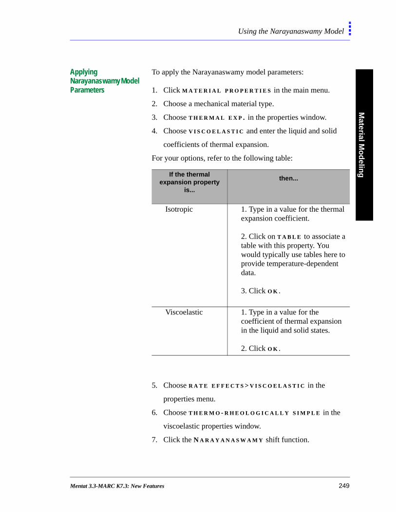
Material M
od
eling
Using the Narayanaswamy Model
Applying Narayanaswamy Model Parameters
To apply the Narayanaswamy model parameters:
1. Click M A T E R I A L P R O P E R T I E S in the main menu.
2. Choose a mechanical material type.
3. Choose T H E R M A L E X P . in the properties window.
4. Choose V I S C O E L A S T I C and enter the liquid and solid
coefficients of thermal expansion.
For your options, refer to the following table:
5. Choose R A T E E F F E C T S > V I S C O E L A S T I C in the
properties menu.
6. Choose T H E R M O - R H E O L O G I C A L L Y S I M P L E in the
viscoelastic properties window.
7. Click the N A R A Y A N A S W A M Y shift function.
If the thermal expansion property
is...
then...
Isotropic 1. Type in a value for the thermal expansion coefficient.
2. Click on T A B L E to associate a table with this property. You would typically use tables here to provide temperature-dependent data.
3. Click O K .
Viscoelastic 1. Type in a value for the coefficient of thermal expansion in the liquid and solid states.
2. Click O K .
Mentat 3.3-MARC K7.3: New Features 249
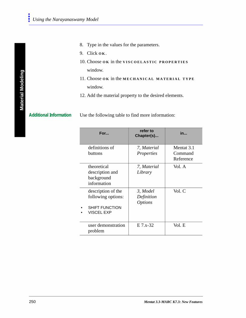
Mat
eria
l Mo
del
ing
Using the Narayanaswamy Model
8. Type in the values for the parameters.
9. Click O K .
10. Choose O K in the V I S C O E L A S T I C P R O P E R T I E S
window.
11. Choose O K in the M E C H A N I C A L M A T E R I A L T Y P E
window.
12. Add the material property to the desired elements.
Additional Information Use the following table to find more information:
For...refer to
Chapter(s)...in...
definitions of buttons
7, Material Properties
Mentat 3.1 Command Reference
theoretical description and background information
7, Material Library
Vol. A
description of the following options:
• SHIFT FUNCTION• VISCEL EXP
3, Model Definition Options
Vol. C
user demonstration problem
E 7.x-32 Vol. E
250 Mentat 3.3-MARC K7.3: New Features
Material M
od
eling
New Approaches in Plasticity Modeling
n
o ble sis
of rge
New Approaches in Plasticity Modeling
Multiplicative Decomposition and New Plasticity Procedures
There are five different plasticity procedures in M A R C :
1. Small Strain–Mean Normal
2. Small Strain–Radial Return
3. Large Strain–Mean Normal–Additive Decomposition
4. Large Strain–Radial Return–Additive Decomposition
5. Large Strain–Radial Return–Multiplicative Decompositio
The difference between the first two procedures is the numerical implementation and determination of the normal tthe yield surface. The Mean-Normal procedure is a more staprocedure, but it usually requires more iterations in the analyprocess. The Radial Return procedure is less stable but in theory, it converges faster.
A new fifth procedure uses the multiplicative decomposition the deformation gradient. This model enables you to take laincrements of strain with greater accuracy and better convergence.
Mentat 3.3-MARC K7.3: New Features 251
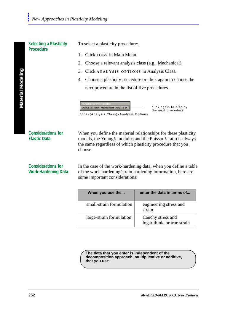
Mat
eria
l Mo
del
ing
New Approaches in Plasticity Modeling
Selecting a Plasticity Procedure
To select a plasticity procedure:
1. Click J O B S in Main Menu.
2. Choose a relevant analysis class (e.g., Mechanical).
3. Click A N A L Y S I S O P T I O N S in Analysis Class.
4. Choose a plasticity procedure or click again to choose the
next procedure in the list of five procedures.
Considerations for Elastic Data
When you define the material relationships for these plasticity models, the Young’s modulus and the Poisson’s ratio is always the same regardless of which plasticity procedure that you choose.
Considerations for Work-Hardening Data
In the case of the work-hardening data, when you define a table of the work-hardening/strain hardening information, here are some important considerations:
c l ick again to d isp laythe next procedure
Jobs>(Analys is Class)>Analys is Opt ions
When you use the... enter the data in terms of...
small-strain formulation engineering stress and strain
large-strain formulation Cauchy stress and logarithmic or true strain
. The data that you enter is independent of the decomposition approach, multiplicative or additive, that you use.
252 Mentat 3.3-MARC K7.3: New Features
Material M
od
eling
New Approaches in Plasticity Modeling
Element Considerations
When a material is in the fully plastic range, the material is almost completely incompressible. This has a consequence on the type of elements that you can use to achieve an accurate solution.
When you use the Large Strain-Mean Normal-Additive Decomposition or the Large Strain-Radial Return-Additive Decomposition, M A R C automatically invokes the Constant Dilatation procedure for lower order elements (types 3, 7, 10, 11, 19, 20). This improves the accuracy of the analysis.
When you use the Large Strain-Radial Return-Multiplicative Decomposition procedure, M A R C uses an alternative, three-field variational approach that is applicable to most displacement-based elements.
For problems involving large strain, avoid using three-node triangular elements or four-node tetrahedral elements.
Mentat 3.3-MARC K7.3: New Features 253
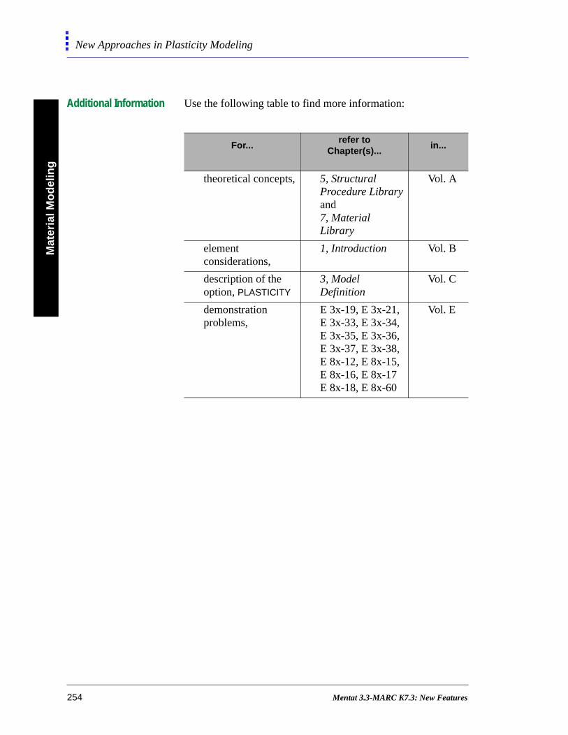
Mat
eria
l Mo
del
ing
New Approaches in Plasticity Modeling
Additional Information Use the following table to find more information:
For...refer to
Chapter(s)...in...
theoretical concepts, 5, Structural Procedure Libraryand7, Material Library
Vol. A
element considerations,
1, Introduction Vol. B
description of the option, PLASTICITY
3, Model Definition
Vol. C
demonstration problems,
E 3x-19, E 3x-21, E 3x-33, E 3x-34,E 3x-35, E 3x-36,E 3x-37, E 3x-38,E 8x-12, E 8x-15,E 8x-16, E 8x-17E 8x-18, E 8x-60
Vol. E
254 Mentat 3.3-MARC K7.3: New Features
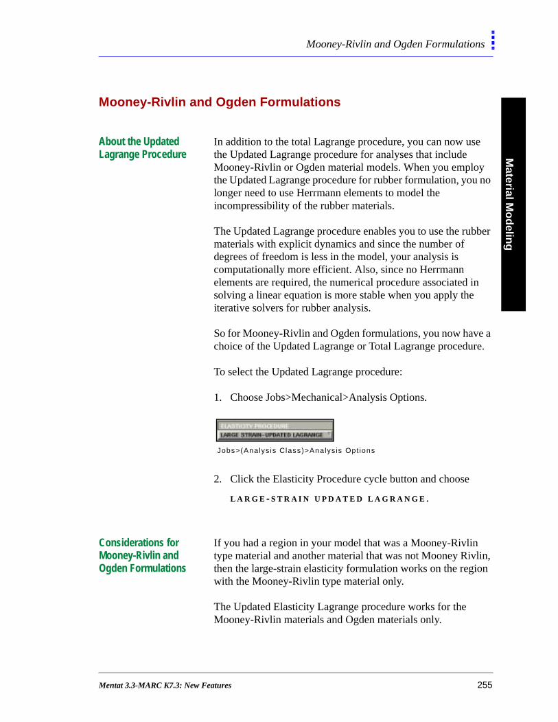
Material M
od
eling
Mooney-Rivlin and Ogden Formulations
Mooney-Rivlin and Ogden Formulations
About the Updated Lagrange Procedure
In addition to the total Lagrange procedure, you can now use the Updated Lagrange procedure for analyses that include Mooney-Rivlin or Ogden material models. When you employ the Updated Lagrange procedure for rubber formulation, you no longer need to use Herrmann elements to model the incompressibility of the rubber materials.
The Updated Lagrange procedure enables you to use the rubber materials with explicit dynamics and since the number of degrees of freedom is less in the model, your analysis is computationally more efficient. Also, since no Herrmann elements are required, the numerical procedure associated in solving a linear equation is more stable when you apply the iterative solvers for rubber analysis.
So for Mooney-Rivlin and Ogden formulations, you now have a choice of the Updated Lagrange or Total Lagrange procedure.
To select the Updated Lagrange procedure:
1. Choose Jobs>Mechanical>Analysis Options.
2. Click the Elasticity Procedure cycle button and choose
L A R G E - S T R A I N U P D A T E D L A G R A N G E .
Considerations for Mooney-Rivlin and Ogden Formulations
If you had a region in your model that was a Mooney-Rivlin type material and another material that was not Mooney Rivlin, then the large-strain elasticity formulation works on the region with the Mooney-Rivlin type material only.
The Updated Elasticity Lagrange procedure works for the Mooney-Rivlin materials and Ogden materials only.
Jobs>(Analys is Class)>Analys is Opt ions
Mentat 3.3-MARC K7.3: New Features 255
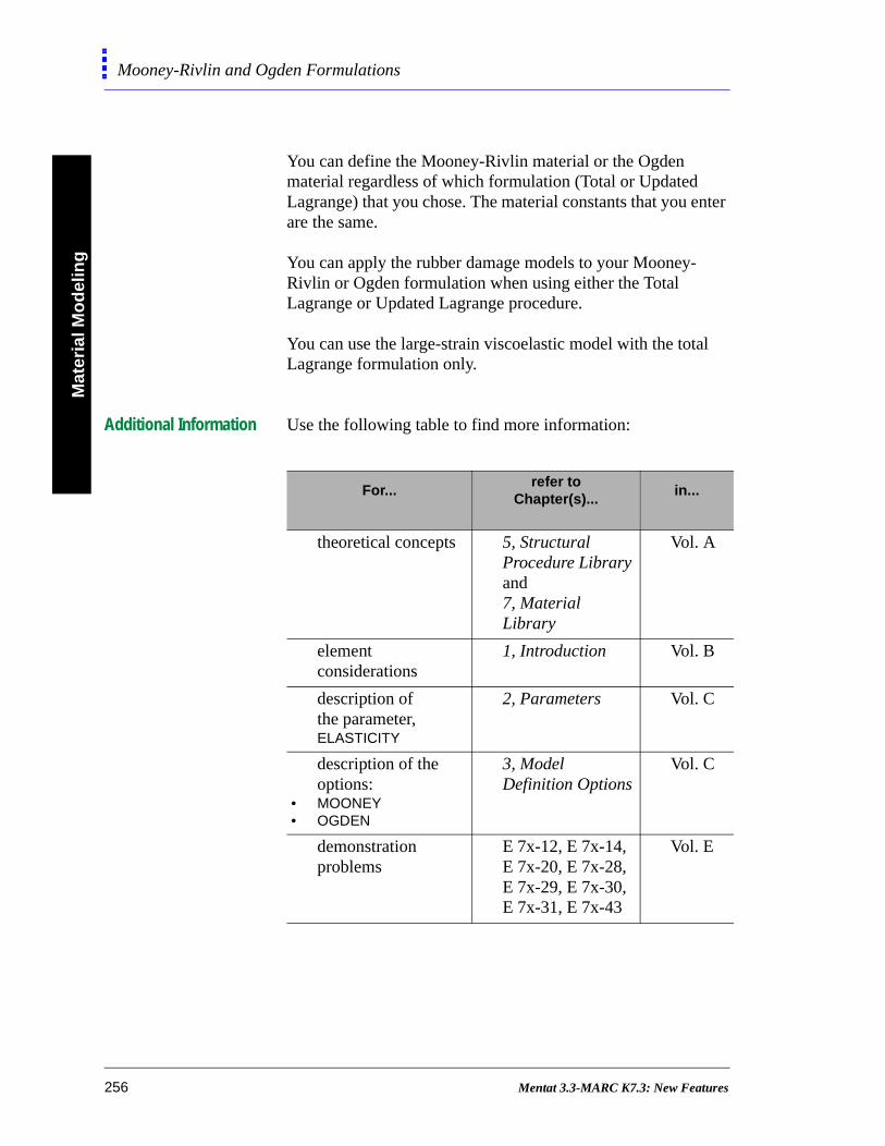
Mat
eria
l Mo
del
ing
Mooney-Rivlin and Ogden Formulations
You can define the Mooney-Rivlin material or the Ogden material regardless of which formulation (Total or Updated Lagrange) that you chose. The material constants that you enter are the same.
You can apply the rubber damage models to your Mooney-Rivlin or Ogden formulation when using either the Total Lagrange or Updated Lagrange procedure.
You can use the large-strain viscoelastic model with the total Lagrange formulation only.
Additional Information Use the following table to find more information:
For...refer to
Chapter(s)...in...
theoretical concepts 5, Structural Procedure Library and7, Material Library
Vol. A
element considerations
1, Introduction Vol. B
description of the parameter, ELASTICITY
2, Parameters Vol. C
description of the options:
• MOONEY • OGDEN
3, Model Definition Options
Vol. C
demonstration problems
E 7x-12, E 7x-14,E 7x-20, E 7x-28,E 7x-29, E 7x-30,E 7x-31, E 7x-43
Vol. E
256 Mentat 3.3-MARC K7.3: New Features
Material M
od
eling
User Subroutines in Hypoelastic Properties
User Subroutines in Hypoelastic Properties
About User Subroutines in Hypoelastic Properties
When you now specify the parameters for hypoelastic material properties, you have the choice of three user subroutines:
• HYPELA
• HYPELA2
• UBEAM
Use HYPELA and HYPELA2 for the following elements:
• continuum elements
• shell elements
• all beam elements except beam elements, 52 and 98
For beam elements 52 and 98, use subroutine, UBEAM (See Vol. D: User Subroutines–UBEAM).
About HYPELA and HYPELA2
HYPELA and HYPELA2 are two user subroutines that you can use with the Hypoelastic option. HYPELA is typically used for elasticity applications. You can use HYPELA2 for modeling arbitrary nonlinear material behavior including elastoplasticity.
For both user subroutines, you should define L and g (where L is a function of the mechanical strain and g is a function of the temperature) such that:
HYPELA2 conveys more information about the kinematics of deformation (i.e., the deformation gradient; stretch ratios: rotation tensor). This enables you to account for rigid rotations while modeling material behavior. Also, you can calculate any kinematic terms that you need to add to the tangent.
σ· ij Li jklε· klgi j+=
Mentat 3.3-MARC K7.3: New Features 257
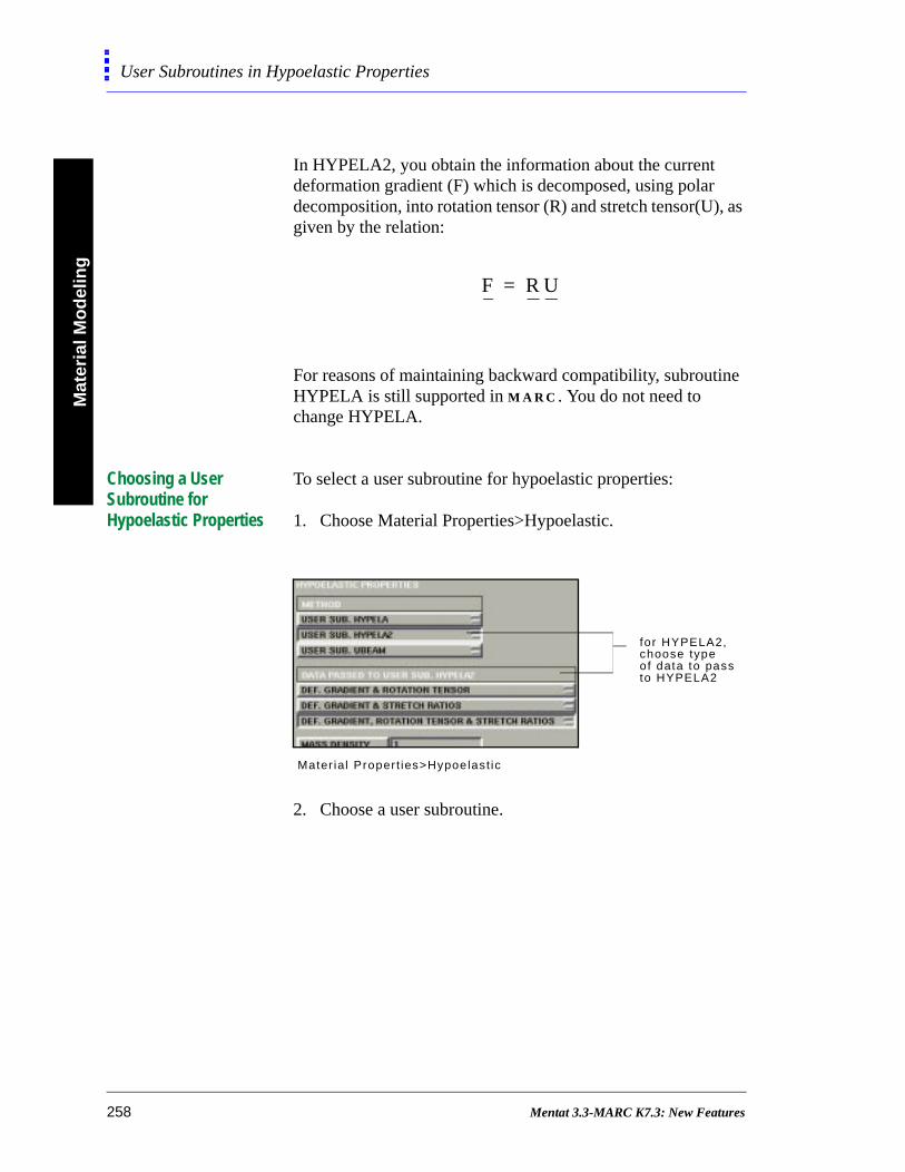
Mat
eria
l Mo
del
ing
User Subroutines in Hypoelastic Properties
In HYPELA2, you obtain the information about the current deformation gradient (F) which is decomposed, using polar decomposition, into rotation tensor (R) and stretch tensor(U), as given by the relation:
For reasons of maintaining backward compatibility, subroutine HYPELA is still supported in M A R C . You do not need to change HYPELA.
Choosing a User Subroutine for Hypoelastic Properties
To select a user subroutine for hypoelastic properties:
1. Choose Material Properties>Hypoelastic.
2. Choose a user subroutine.
F R U=
for HYPELA2, choose typeof data to passto HYPELA2
Mater ial Proper t ies>Hypoelast ic
258 Mentat 3.3-MARC K7.3: New Features
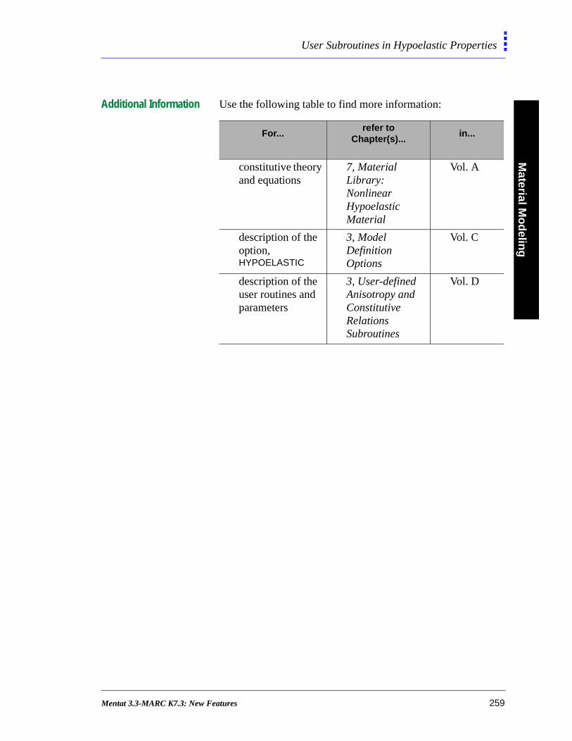
Material M
od
eling
User Subroutines in Hypoelastic Properties
Additional Information Use the following table to find more information:
For...refer to
Chapter(s)...in...
constitutive theory and equations
7, Material Library: Nonlinear Hypoelastic Material
Vol. A
description of the option,HYPOELASTIC
3, Model Definition Options
Vol. C
description of the user routines and parameters
3, User-defined Anisotropy and Constitutive Relations Subroutines
Vol. D
Mentat 3.3-MARC K7.3: New Features 259
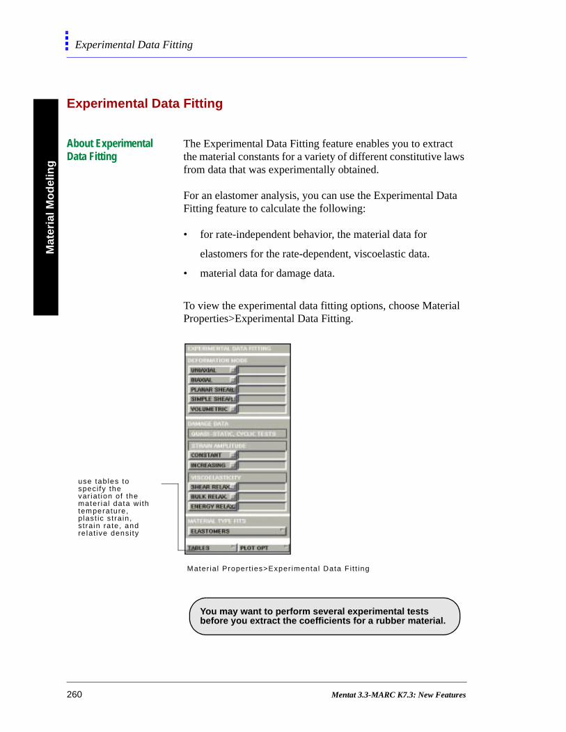
Mat
eria
l Mo
del
ing
Experimental Data Fitting
al
Experimental Data Fitting
About Experimental Data Fitting
The Experimental Data Fitting feature enables you to extract the material constants for a variety of different constitutive laws from data that was experimentally obtained.
For an elastomer analysis, you can use the Experimental Data Fitting feature to calculate the following:
• for rate-independent behavior, the material data for
elastomers for the rate-dependent, viscoelastic data.
• material data for damage data.
To view the experimental data fitting options, choose MateriProperties>Experimental Data Fitting.
use tab les to specify the var iat ion of the mater ial data wi thtemperature, plast ic s tra in ,strain ra te, andre lat ive density
Mater ial Propert ies>Exper imenta l Data F i t t ing
You may want to perform several experimental testsbefore you extract the coefficients for a rubber material.
260 Mentat 3.3-MARC K7.3: New Features

Material M
od
eling
Experimental Data Fitting
d
s ot
About Experimental Tests
The Experimental Data Fitting menus feature the following deformation modes for calibrating quasi-static stress-strain response curves (See also Mentat Command Reference, Chap. 7: Experimental Data Fitting):
• uniaxial
• biaxial
• planar shear (or pure shear)
• simple shear
• volumetric
While it is possible to use just uniaxial data for curve fitting anextract the constants for elastomeric material models, you should also have experimental data for multiple types of experiments. This enables you to achieve material constantthat can be used in practical engineering analysis. You cannuse shear experimental data for obtaining constants for the Foam model.
Reading in Experimental Data
Using the Experimental Data Fitting menus, you can read inyour experimental data in a tabular form containing the engineering strain (ε) and the engineering stress (σ) measures. The Foam model requires dilatational information (See “About Forms of Data” on page 262). The experimental data is read in as ε, σ, J (Jacobian of deformation).
To read in your experimental data:
1. Choose Material Properties>Experimental Data Fitting.
cl ick to d isp lay the current ly-def ined exper imenta l datatab les
Mater ia l Propert ies>Exper imenta l Data Fi t t ing
Mentat 3.3-MARC K7.3: New Features 261
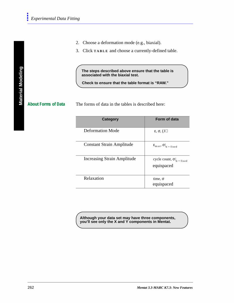
Mat
eria
l Mo
del
ing
Experimental Data Fitting
2. Choose a deformation mode (e.g., biaxial).
3. Click T A B L E and choose a currently-defined table.
About Forms of Data The forms of data in the tables is described here:
.
Check to ensure that the table format is “RAW.”
The steps described above ensure that the table is associated with the biaxial test.
Category Form of data
Deformation Mode
Constant Strain Amplitude
Increasing Strain Amplitude
equispaced
Relaxationequispaced
ε σ J( ), ,
εmax σ ε fixed=,
cycle count σ ε fixed=,
time σ,
. Although your data set may have three components,you’ll see only the X and Y components in Mentat.
262 Mentat 3.3-MARC K7.3: New Features

Material M
od
eling
Experimental Data Fitting
For Foam models, the Z-component is the dilatational information, (J). The relation between the deformation mode and form of J is given below:
Deformation J where:
uniaxial A is the cross-sectional area:
biaxial t is the thickness of the sheet:
A A0⁄
A
t t0⁄
t
Mentat 3.3-MARC K7.3: New Features 263
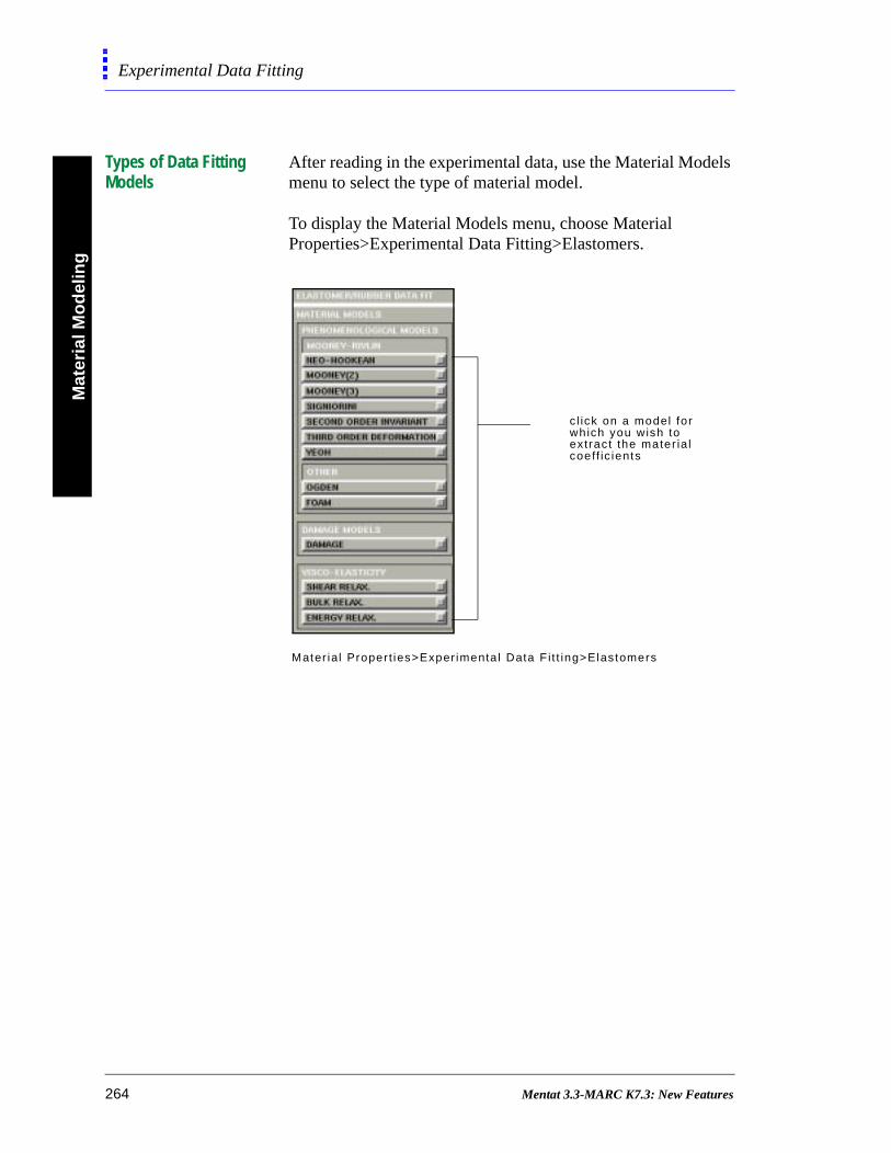
Mat
eria
l Mo
del
ing
Experimental Data Fitting
Types of Data Fitting Models
After reading in the experimental data, use the Material Models menu to select the type of material model.
To display the Material Models menu, choose Material Properties>Experimental Data Fitting>Elastomers.
extract the mater ia l
c l ick on a model forwhich you wish to
coeff ic ients
Mater ial Propert ies>Exper imenta l Data F i t t ing>Elastomers
264 Mentat 3.3-MARC K7.3: New Features
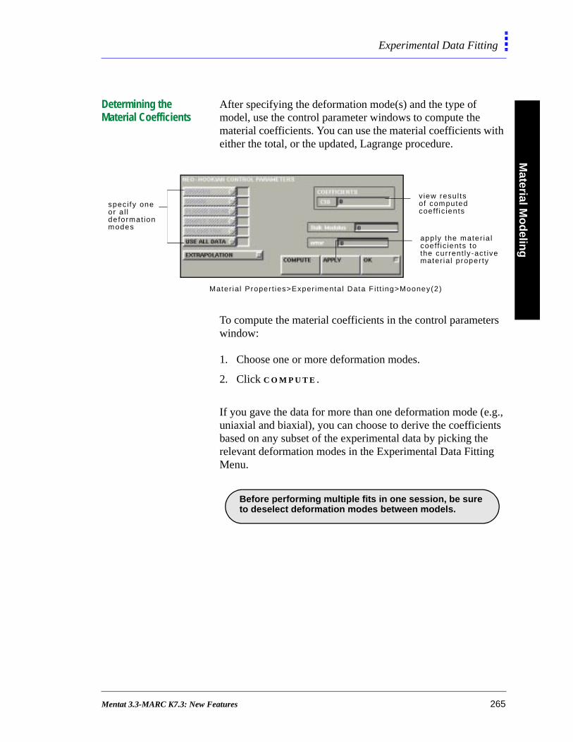
Material M
od
eling
Experimental Data Fitting
Determining the Material Coefficients
After specifying the deformation mode(s) and the type of model, use the control parameter windows to compute the material coefficients. You can use the material coefficients with either the total, or the updated, Lagrange procedure.
To compute the material coefficients in the control parameters window:
1. Choose one or more deformation modes.
2. Click C O M P U T E .
If you gave the data for more than one deformation mode (e.g., uniaxial and biaxial), you can choose to derive the coefficients based on any subset of the experimental data by picking the relevant deformation modes in the Experimental Data Fitting Menu.
view resul tsof computedcoeff ic ients
specify oneor a l l deformat ionmodes
Mater ial Proper t ies>Exper imenta l Data F i t t ing>Mooney(2)
apply the mater ia lcoeff ic ients to the current ly-act ivemater ial proper ty
. Before performing multiple fits in one session, be sure to deselect deformation modes between models.
Mentat 3.3-MARC K7.3: New Features 265
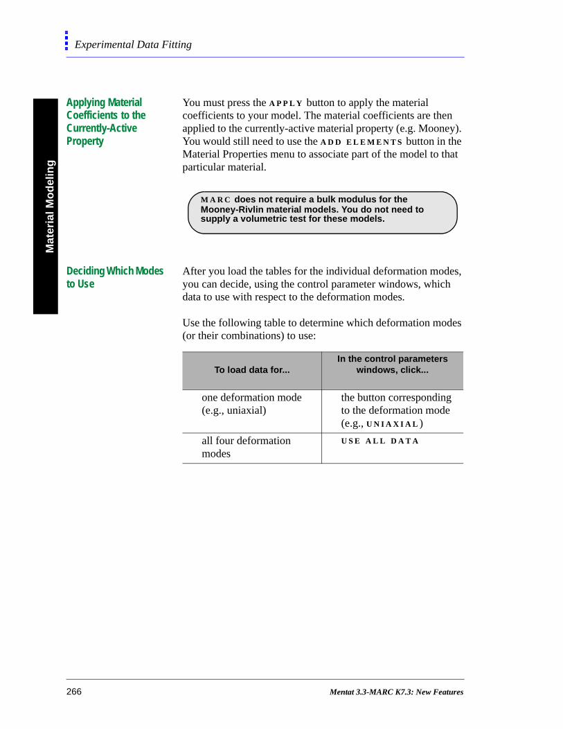
Mat
eria
l Mo
del
ing
Experimental Data Fitting
Applying Material Coefficients to the Currently-Active Property
You must press the A P P L Y button to apply the material coefficients to your model. The material coefficients are then applied to the currently-active material property (e.g. Mooney). You would still need to use the A D D E L E M E N T S button in the Material Properties menu to associate part of the model to that particular material.
Deciding Which Modes to Use
After you load the tables for the individual deformation modes, you can decide, using the control parameter windows, which data to use with respect to the deformation modes.
Use the following table to determine which deformation modes (or their combinations) to use:
. M A R C does not require a bulk modulus for the
Mooney-Rivlin material models. You do not need tosupply a volumetric test for these models.
To load data for...In the control parameters
windows, click...
one deformation mode (e.g., uniaxial)
the button corresponding to the deformation mode (e.g., U N I A X I A L )
all four deformation modes
U S E A L L D A T A
266 Mentat 3.3-MARC K7.3: New Features
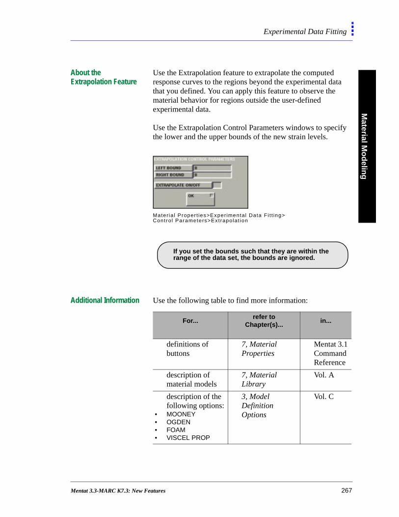
Material M
od
eling
Experimental Data Fitting
About the Extrapolation Feature
Use the Extrapolation feature to extrapolate the computed response curves to the regions beyond the experimental data that you defined. You can apply this feature to observe the material behavior for regions outside the user-defined experimental data.
Use the Extrapolation Control Parameters windows to specify the lower and the upper bounds of the new strain levels.
Additional Information Use the following table to find more information:
Materia l Proper t ies>Exper imental Data Fi t t ing>Contro l Parameters>Extrapolat ion
. If you set the bounds such that they are within the
range of the data set, the bounds are ignored.
For...refer to
Chapter(s)...in...
definitions of buttons
7, Material Properties
Mentat 3.1 Command Reference
description of material models
7, Material Library
Vol. A
description of the following options:
• MOONEY• OGDEN• FOAM• VISCEL PROP
3, Model Definition Options
Vol. C
Mentat 3.3-MARC K7.3: New Features 267
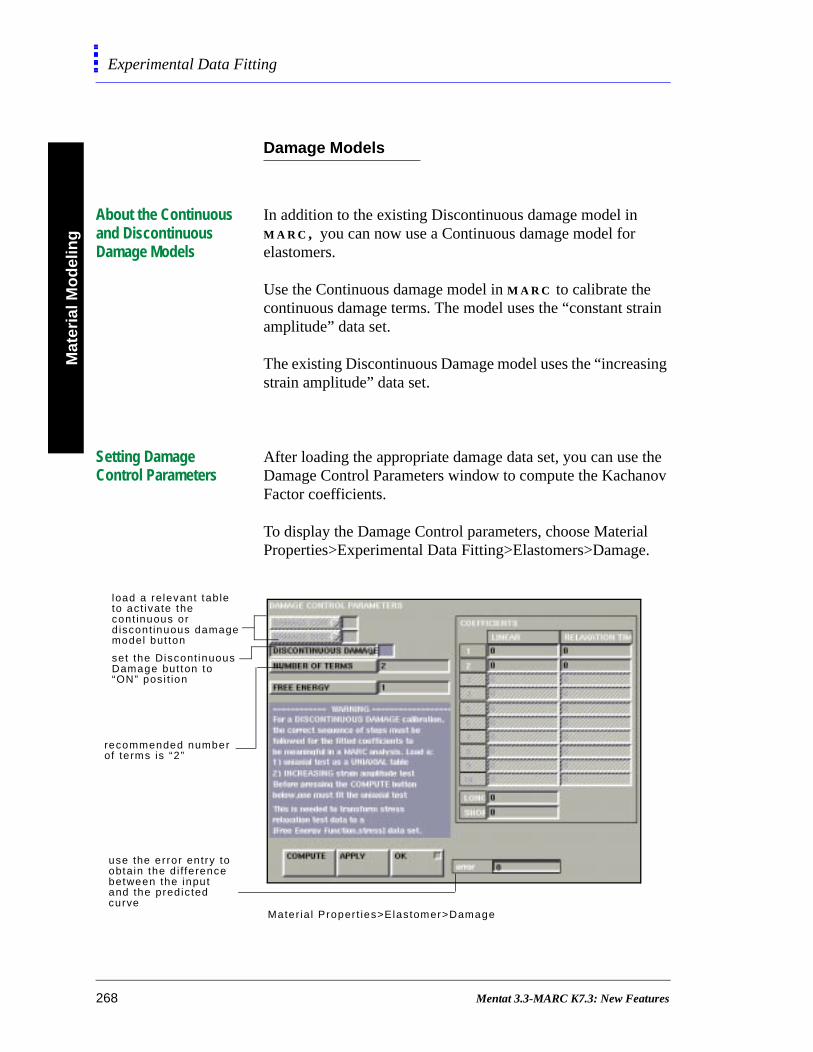
Mat
eria
l Mo
del
ing
Experimental Data Fitting
rain
ing
the nov
l .
Damage Models
About the Continuous and Discontinuous Damage Models
In addition to the existing Discontinuous damage model in M A R C , you can now use a Continuous damage model for elastomers.
Use the Continuous damage model in M A R C to calibrate the continuous damage terms. The model uses the “constant stamplitude” data set.
The existing Discontinuous Damage model uses the “increasstrain amplitude” data set.
Setting Damage Control Parameters
After loading the appropriate damage data set, you can useDamage Control Parameters window to compute the KachaFactor coefficients.
To display the Damage Control parameters, choose MateriaProperties>Experimental Data Fitting>Elastomers>Damage
load a relevant tab leto act ivate the cont inuous or d iscont inuous damagemodel but ton
use the error entry to obtain the d i fferencebetween the inputand the predic tedcurve
recommended numberof terms is “2”
Mater ia l Proper t ies>Elastomer>Damage
set the Discont inuous
“ON” posi t ion Damage button to
268 Mentat 3.3-MARC K7.3: New Features
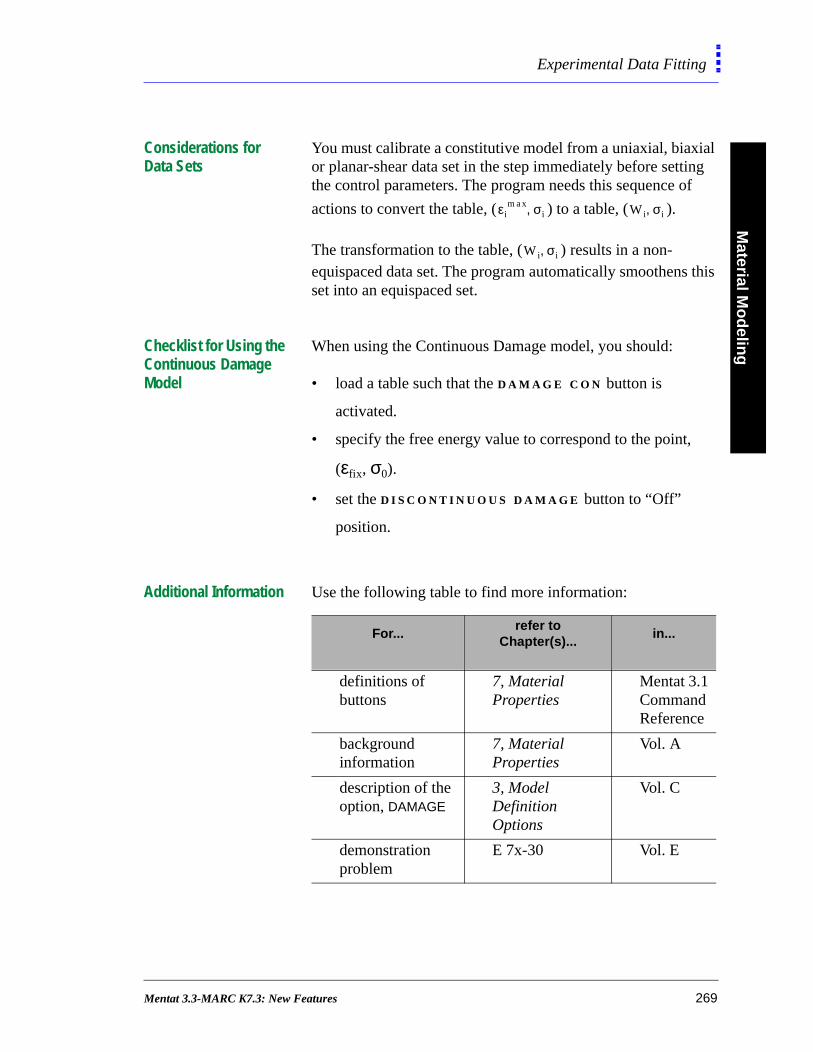
Material M
od
eling
Experimental Data Fitting
Considerations for Data Sets
You must calibrate a constitutive model from a uniaxial, biaxial or planar-shear data set in the step immediately before setting the control parameters. The program needs this sequence of
actions to convert the table, ( ) to a table, ( ).
The transformation to the table, ( ) results in a non-equispaced data set. The program automatically smoothens this set into an equispaced set.
Checklist for Using the Continuous Damage Model
When using the Continuous Damage model, you should:
• load a table such that the D A M A G E C O N button is
activated.
• specify the free energy value to correspond to the point,
(εfix, σ0).
• set the D I S C O N T I N U O U S D A M A G E button to “Off”
position.
Additional Information Use the following table to find more information:
εimax σi, Wi σi,
Wi σi,
For...refer to
Chapter(s)...in...
definitions of buttons
7, Material Properties
Mentat 3.1 Command Reference
background information
7, Material Properties
Vol. A
description of the option, DAMAGE
3, Model Definition Options
Vol. C
demonstration problem
E 7x-30 Vol. E
Mentat 3.3-MARC K7.3: New Features 269
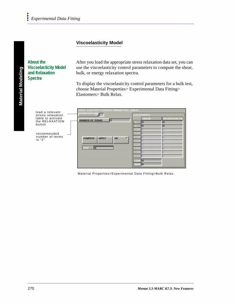
Mat
eria
l Mo
del
ing
Experimental Data Fitting
Viscoelasticity Model
About the Viscoelasticity Model and Relaxation Spectra
After you load the appropriate stress relaxation data set, you can use the viscoelasticity control parameters to compute the shear, bulk, or energy relaxation spectra.
To display the viscoelasticity control parameters for a bulk test, choose Material Properties> Experimental Data Fitting> Elastomers> Bulk Relax.
load a re levantstress relaxat ion table to act ivatethe RELAXATIONbutton
recommendednumber of termsi s “2”
Mater ia l Proper t ies>Exper imenta l Data Fi t t ing>Bulk Relax.
270 Mentat 3.3-MARC K7.3: New Features
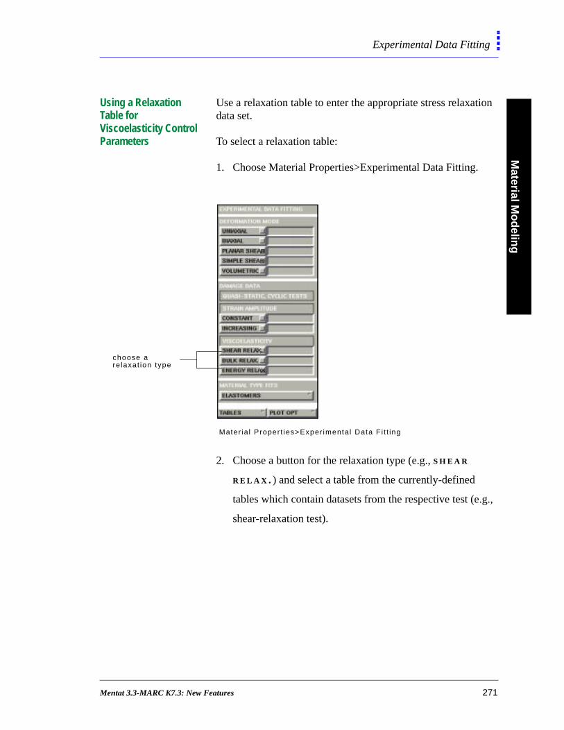
Material M
od
eling
Experimental Data Fitting
Using a Relaxation Table for Viscoelasticity Control Parameters
Use a relaxation table to enter the appropriate stress relaxation data set.
To select a relaxation table:
1. Choose Material Properties>Experimental Data Fitting.
2. Choose a button for the relaxation type (e.g., S H E A R
R E L A X . ) and select a table from the currently-defined
tables which contain datasets from the respective test (e.g.,
shear-relaxation test).
Mater ial Propert ies>Exper imental Data F i t t ing
choose a re laxat ion type
Mentat 3.3-MARC K7.3: New Features 271

Mat
eria
l Mo
del
ing
Experimental Data Fitting
Computing the Coefficients for Shear, or Bulk Relaxation Tests
Use the Viscoelasticity Control Parameters window to compute the coefficients for shear, or bulk relaxation tests.
To compute the coefficients:
1. Choose Material Properties>Experimental Data
Fitting>Elastomers.
2. Choose either the S H E A R R E L A X . or the B U L K R E L A X .
button.
3. Click C O M P U T E .
Determining the Coefficients for an Energy Relaxation Test
Use the Viscoelasticity Control Parameters (Free Energy) window to compute the coefficients for an energy relaxation test.
To compute the coefficients:
1. Choose Material Properties>Experimental Data
Fitting>Elastomers.
2. Click E N E R G Y R E L A X .
3. Click C O M P U T E .
Considerations for Data Sets
You must calibrate a constitutive model from a uniaxial test in the step immediately before setting the control parameters. The program requires this sequence of actions to convert the table, ( ) to a table, ( ) where .timei σi, timei Wi, i 1 2 3,...N, ,=
272 Mentat 3.3-MARC K7.3: New Features
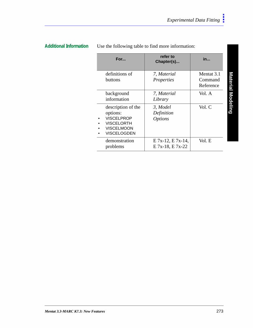
Material M
od
eling
Experimental Data Fitting
Additional Information Use the following table to find more information:
For...refer to
Chapter(s)...in...
definitions of buttons
7, Material Properties
Mentat 3.1 Command Reference
background information
7, Material Library
Vol. A
description of the options:
• VISCELPROP• VISCELORTH• VISCELMOON• VISCELOGDEN
3, Model Definition Options
Vol. C
demonstration problems
E 7x-12, E 7x-14,E 7x-18, E 7x-22
Vol. E
Mentat 3.3-MARC K7.3: New Features 273

Mentat 3.3-MARC K7.3: New Features

11•Analysis Integration
Using Radiation Viewfactors
About the Radiation View Factor Feature 277Applying Radiation As Boundary Conditions 278About Emitting and Incident Objects 279About the Compute Radiation Viewfactors Window 280Computing Viewfactors in Analysis 283
Mentat 3.3-MARC K7.3: New Features 275

• Analysis Integration
Mentat 3.3-MARC K7.3: New Features
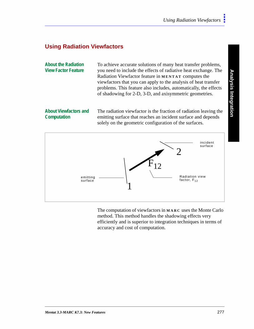
An
alysis Integ
ration
Using Radiation Viewfactors
Using Radiation Viewfactors
About the Radiation View Factor Feature
To achieve accurate solutions of many heat transfer problems, you need to include the effects of radiative heat exchange. The Radiation Viewfactor feature in M E N T A T computes the viewfactors that you can apply to the analysis of heat transfer problems. This feature also includes, automatically, the effects of shadowing for 2-D, 3-D, and axisymmetric geometries.
About Viewfactors and Computation
The radiation viewfactor is the fraction of radiation leaving the emitting surface that reaches an incident surface and depends solely on the geometric configuration of the surfaces.
The computation of viewfactors in M A R C uses the Monte Carlo method. This method handles the shadowing effects very efficiently and is superior to integration techniques in terms of accuracy and cost of computation.
1
2F12
inc identsur face
emit t ingsur face
Radiat ion viewfactor, F12
Mentat 3.3-MARC K7.3: New Features 277
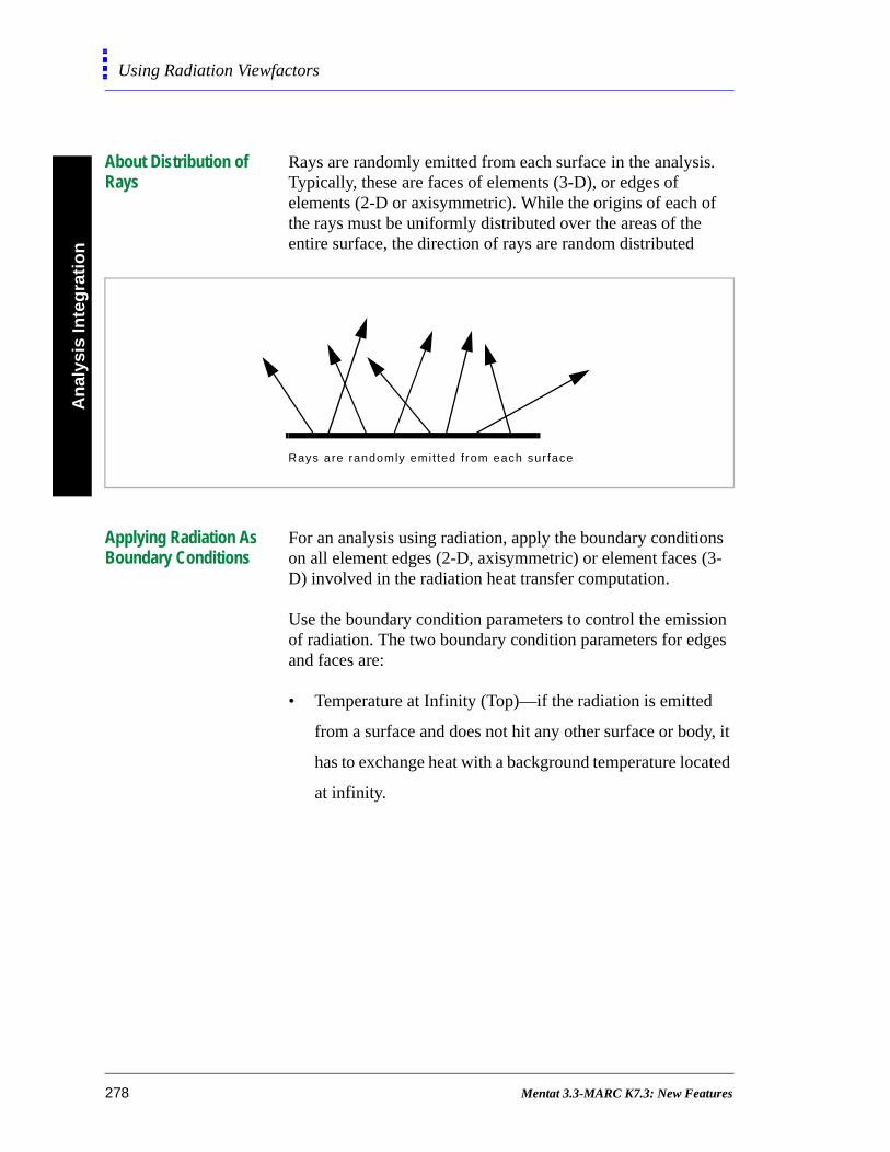
An
alys
is In
teg
rati
on
Using Radiation Viewfactors
y, it
ated
About Distribution of Rays
Rays are randomly emitted from each surface in the analysis. Typically, these are faces of elements (3-D), or edges of elements (2-D or axisymmetric). While the origins of each of the rays must be uniformly distributed over the areas of the entire surface, the direction of rays are random distributed
Applying Radiation As Boundary Conditions
For an analysis using radiation, apply the boundary conditions on all element edges (2-D, axisymmetric) or element faces (3-D) involved in the radiation heat transfer computation.
Use the boundary condition parameters to control the emission of radiation. The two boundary condition parameters for edges and faces are:
• Temperature at Infinity (Top)—if the radiation is emitted
from a surface and does not hit any other surface or bod
has to exchange heat with a background temperature loc
at infinity.
Rays are randomly emi t ted f rom each sur face
278 Mentat 3.3-MARC K7.3: New Features
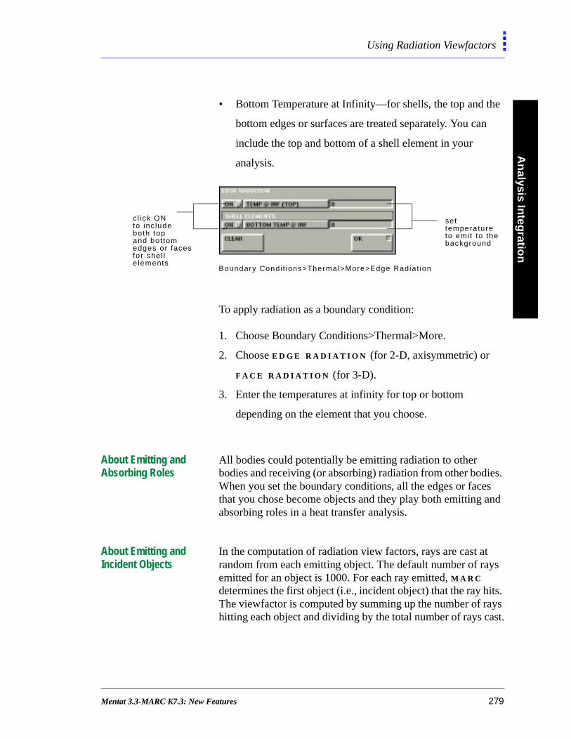
An
alysis Integ
ration
Using Radiation Viewfactors
e
n
es. s
and
ys
its. ys
ast.
• Bottom Temperature at Infinity—for shells, the top and th
bottom edges or surfaces are treated separately. You ca
include the top and bottom of a shell element in your
analysis.
To apply radiation as a boundary condition:
1. Choose Boundary Conditions>Thermal>More.
2. Choose E D G E R A D I A T I O N (for 2-D, axisymmetric) or
F A C E R A D I A T I O N (for 3-D).
3. Enter the temperatures at infinity for top or bottom
depending on the element that you choose.
About Emitting and Absorbing Roles
All bodies could potentially be emitting radiation to other bodies and receiving (or absorbing) radiation from other bodiWhen you set the boundary conditions, all the edges or facethat you chose become objects and they play both emitting absorbing roles in a heat transfer analysis.
About Emitting and Incident Objects
In the computation of radiation view factors, rays are cast atrandom from each emitting object. The default number of raemitted for an object is 1000. For each ray emitted, M A R C determines the first object (i.e., incident object) that the ray hThe viewfactor is computed by summing up the number of rahitting each object and dividing by the total number of rays c
settemperatureto emit to thebackground
cl ick ONto inc ludeboth topand bottomedges or facesfor shel le lements
Boundary Condi t ions>Thermal>More>Edge Radiat ion
Mentat 3.3-MARC K7.3: New Features 279

An
alys
is In
teg
rati
on
Using Radiation Viewfactors
About the Compute Radiation Viewfactors Window
Use the Compute Radiation Viewfactors window to specify the parameters for the computation of viewfactors.
To specify the parameters, choose Jobs>Radiation Viewfactors.
Jobs>Radiat ion Viewfactors
number ofp lanesvary withyour choiceof geometrytype
280 Mentat 3.3-MARC K7.3: New Features
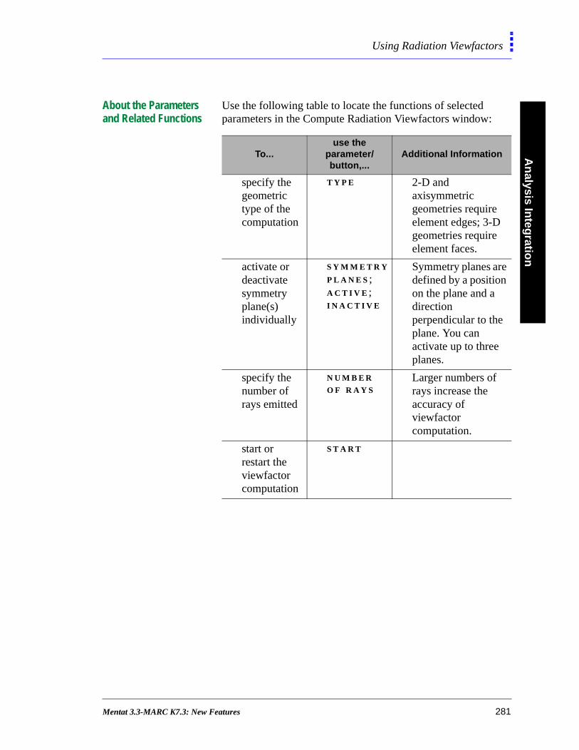
An
alysis Integ
ration
Using Radiation Viewfactors
About the Parameters and Related Functions
Use the following table to locate the functions of selected parameters in the Compute Radiation Viewfactors window:
To...use the
parameter/button,...
Additional Information
specify the geometric type of the computation
T Y P E 2-D and axisymmetric geometries require element edges; 3-D geometries require element faces.
activate or deactivate symmetry plane(s) individually
S Y M M E T R Y P L A N E S ; A C T I V E ; I N A C T I V E
Symmetry planes are defined by a position on the plane and a direction perpendicular to the plane. You can activate up to three planes.
specify the number of rays emitted
N U M B E R O F R A Y S
Larger numbers of rays increase the accuracy of viewfactor computation.
start or restart the viewfactor computation
S T A R T
Mentat 3.3-MARC K7.3: New Features 281
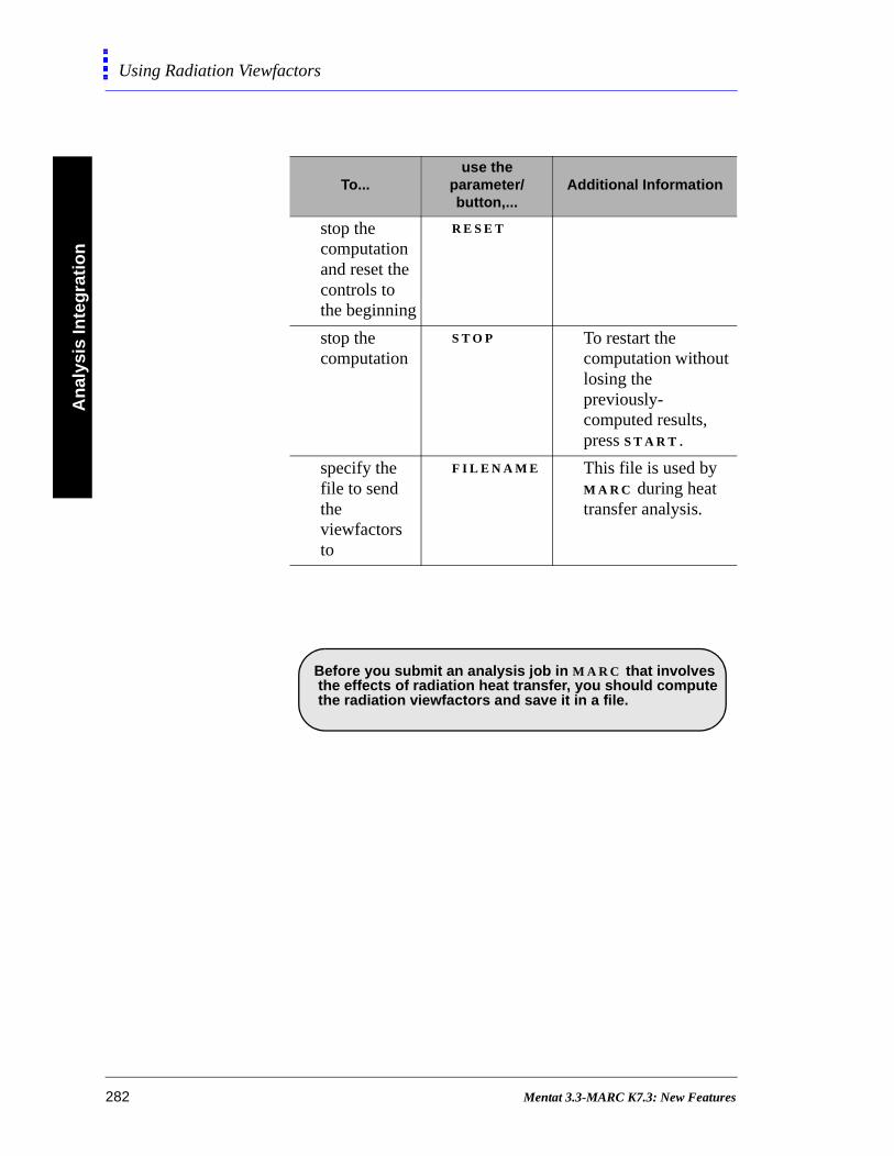
An
alys
is In
teg
rati
on
Using Radiation Viewfactors
stop the computation and reset the controls to the beginning
R E S E T
stop the computation
S T O P To restart the computation without losing the previously- computed results, press S T A R T .
specify the file to send the viewfactors to
F I L E N A M E This file is used by M A R C during heat transfer analysis.
To...use the
parameter/button,...
Additional Information
.
Before you submit an analysis job in M A R C that involves the effects of radiation heat transfer, you should compute the radiation viewfactors and save it in a file.
282 Mentat 3.3-MARC K7.3: New Features

An
alysis Integ
ration
Using Radiation Viewfactors
Computing Viewfactors in Analysis
To compute the radiation viewfactors for existing radiation boundary conditions:
1. Choose Jobs>Radiation Viewfactors.
2. Choose the type (geometry) based on whether you set edges
(2-D; axisymmetric) or faces (3-D) for your radiation
boundary conditions.
3. If you wish to use symmetry planes, click on A C T I V E in
Symmetry Plane to activate the plane(s); use the N O R M A L
and P O S I T I O N buttons to define the plane(s).
4. Click F I L E N A M E and specify a name of the file to store
your results in.
5. Specify the number of emitted rays to be used for each
element edge or face.
6. Click S T A R T .
Indicating the Location of the Viewfactor File
When you submit the heat transfer analysis through M E N T A T , the location of the viewfactor file is provided to M A R C .
When you use the M A R C shell script to run the analysis, use the -vf filename option to indicate the location of the viewfactor file.
If you defined edges only and you click 3-D as your choice of T Y P E , the number of objects in the O B J E C T S field will be zero.
Mentat 3.3-MARC K7.3: New Features 283
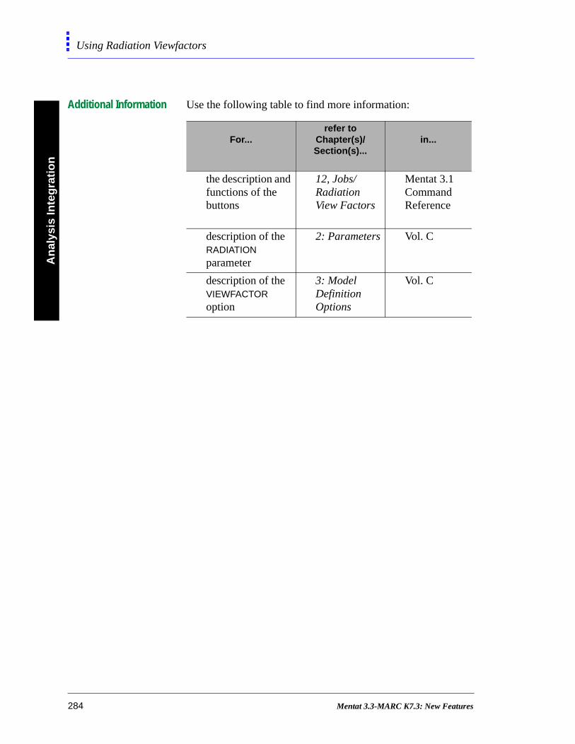
An
alys
is In
teg
rati
on
Using Radiation Viewfactors
Additional Information Use the following table to find more information:
For...refer to
Chapter(s)/Section(s)...
in...
the description and functions of the buttons
12, Jobs/Radiation View Factors
Mentat 3.1 Command Reference
description of the RADIATION parameter
2: Parameters Vol. C
description of the VIEWFACTOR option
3: Model Definition Options
Vol. C
284 Mentat 3.3-MARC K7.3: New Features

Appendixes
A: User Enhancements 287B: Fluid Elements 293C: MARC Data Reader Support 297D: NASTRAN Writer Data Entries 305E: Command Line Parameters 315F: Demonstration Problems 321
Mentat 3.3-MARC K7.3: New Features 285

• Appendixes, A-F
Mentat 3.3-MARC K7.3: New Features
A: User Enhancements
List of User Enhancements
MARC New Parameters 289MARC New Model Definition 289MARC New History Definition 290New User Subroutines 290New Element Types 290
Mentat 3.3-MARC K7.3: New Features 287
• Appendix A: User Enhancements
Mentat 3.3-MARC K7.3: New Features
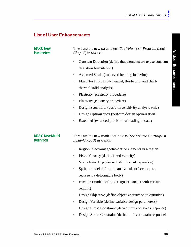
A: U
ser En
han
cemen
tsList of User Enhancements
tant
e)
)
List of User Enhancements
MARC New Parameters
These are the new parameters (See Volume C: Program Input–Chap. 2) in M A R C :
• Constant Dilatation (define that elements are to use cons
dilatation formulation)
• Assumed Strain (improved bending behavior)
• Fluid (for fluid, fluid-thermal, fluid-solid, and fluid-
thermal-solid analysis)
• Plasticity (plasticity procedure)
• Elasticity (elasticity procedure)
• Design Sensitivity (perform sensitivity analysis only)
• Design Optimization (perform design optimization)
• Extended (extended precision of reading in data)
MARC New Model Definition
These are the new model definitions (See Volume C: Program Input–Chap. 3) in M A R C :
• Region (electromagnetic–define elements in a region)
• Fixed Velocity (define fixed velocity)
• Viscoelastic Exp (viscoelastic thermal expansion)
• Spline (model definition–analytical surface used to
represent a deformable body)
• Exclude (model definition–ignore contact with certain
regions)
• Design Objective (define objective function to optimize)
• Design Variable (define variable design parameters)
• Design Stress Constraint (define limits on stress respons
• Design Strain Constraint (define limits on strain response
Mentat 3.3-MARC K7.3: New Features 289

A:
Use
r E
nh
ance
men
tsList of User Enhancements
les:
)
• Design Frequency Constraint (define limits on
eigenfrequency response)
• Design Displacement Constraint (define limits on
displacement response)
MARC New History Definition
These are the new history definitions (See Volume C, Chapter 4–History Definition: Static, Dynamic, Creep Analysis.) in M A R C :
• Auto Step (adaptive load step control)
• Approach (move rigid surfaces into position)
• Synchronize (move rigid surfaces into position)
New User Subroutines Here are the new user subroutines (See Volume D: User Subroutines) in M A R C :
• UPSTRECH (definition of generalized principal stretch-
based elasticity models: See Chap. 3)
• HYPELA2 (user-defined material behavior: See Chap. 3)
• UPOSTV (user-selected post-processing of nodal variab
See Chap. 7)
• UFINITE (finite deformation isotropic material models: See
Chap. 3)
New Element Types Here are the new element types (See Volume B: Element Library–Chap. 3) available in M A R C :
• 138 (bilinear thin-triangular shell element)
• 139 (bilinear thin-shell Element)
• 140 (bilinear thick-shell element with reduced integration
• 142 (eight-node axisymmetric rebar element with twist)
290 Mentat 3.3-MARC K7.3: New Features
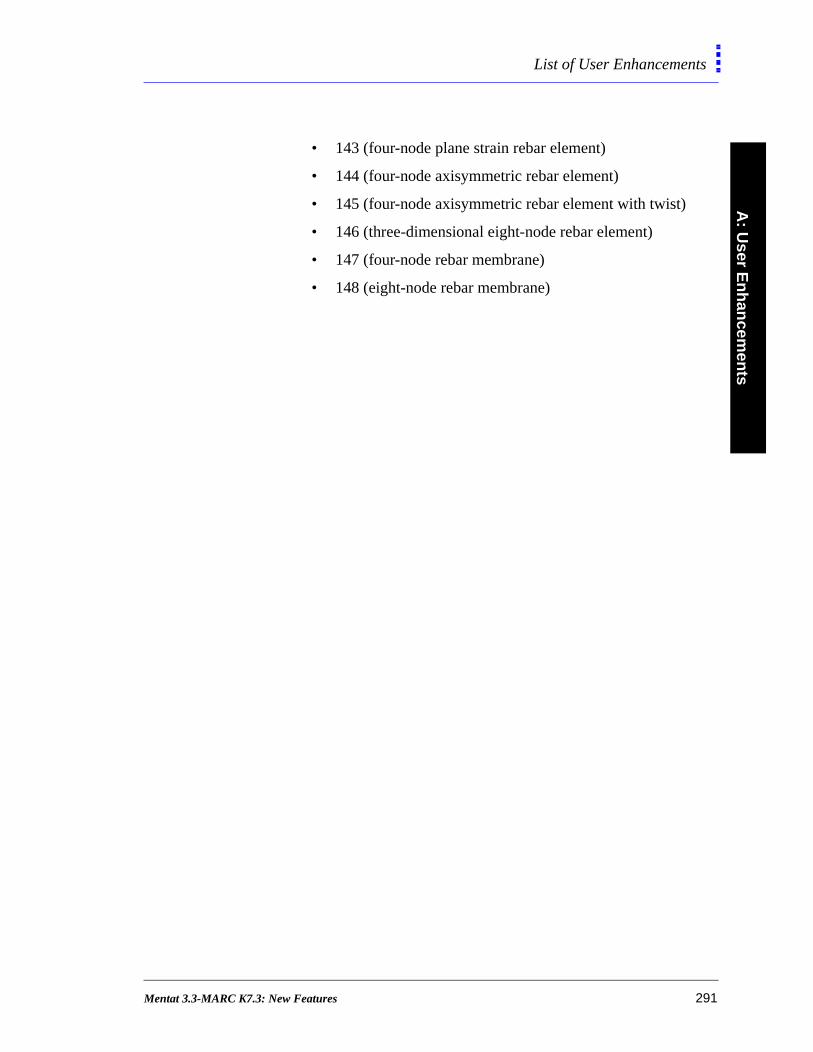
A: U
ser En
han
cemen
tsList of User Enhancements
• 143 (four-node plane strain rebar element)
• 144 (four-node axisymmetric rebar element)
• 145 (four-node axisymmetric rebar element with twist)
• 146 (three-dimensional eight-node rebar element)
• 147 (four-node rebar membrane)
• 148 (eight-node rebar membrane)
Mentat 3.3-MARC K7.3: New Features 291

Mentat 3.3-MARC K7.3: New Features
B: Fluid Elements
Fluid Element Types
Planar Element Types 295Axisymmetric Element Types 295Three-Dimensional Element Types 296
Mentat 3.3-MARC K7.3: New Features 293

• Fluid Elements
Mentat 3.3-MARC K7.3: New Features
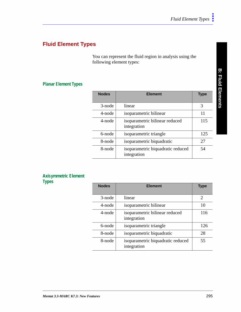
B: F
luid
Elem
ents
Fluid Element Types
Fluid Element Types
You can represent the fluid region in analysis using the following element types:
Planar Element Types
Axisymmetric Element Types
Nodes Element Type
3-node linear 3
4-node isoparametric bilinear 11
4-node isoparametric bilinear reduced integration
115
6-node isoparametric triangle 125
8-node isoparametric biquadratic 27
8-node isoparametric biquadratic reduced integration
54
Nodes Element Type
3-node linear 2
4-node isoparametric bilinear 10
4-node isoparametric bilinear reduced integration
116
6-node isoparametric triangle 126
8-node isoparametric biquadratic 28
8-node isoparametric biquadratic reduced integration
55
Mentat 3.3-MARC K7.3: New Features 295
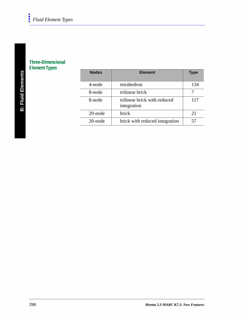
B:
Flu
id E
lem
ents
Fluid Element Types
Three-Dimensional Element Types
Nodes Element Type
4-node tetrahedron 134
8-node trilinear brick 7
8-node trilinear brick with reduced integration
117
20-node brick 21
20-node brick with reduced integration 57
296 Mentat 3.3-MARC K7.3: New Features
C: MARC Data Reader Support
Supported Parameters
List of Supported Parameters 299
Supported Model-Definition Options
List of Supported Model-Definition Options 301
Mentat 3.3-MARC K7.3: New Features 297

• MARC Data Reader Support
Mentat 3.3-MARC K7.3: New Features
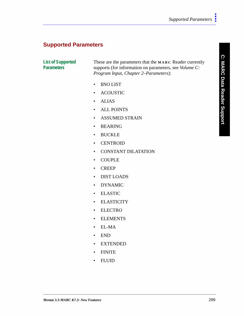
C: M
AR
C D
ata Read
er Su
pp
ort
Supported Parameters
Supported Parameters
List of Supported Parameters
These are the parameters that the M A R C Reader currently supports (for information on parameters, see Volume C: Program Input, Chapter 2–Parameters):
• $NO LIST
• ACOUSTIC
• ALIAS
• ALL POINTS
• ASSUMED STRAIN
• BEARING
• BUCKLE
• CENTROID
• CONSTANT DILATATION
• COUPLE
• CREEP
• DIST LOADS
• DYNAMIC
• ELASTIC
• ELASTICITY
• ELECTRO
• ELEMENTS
• EL-MA
• END
• EXTENDED
• FINITE
• FLUID
Mentat 3.3-MARC K7.3: New Features 299
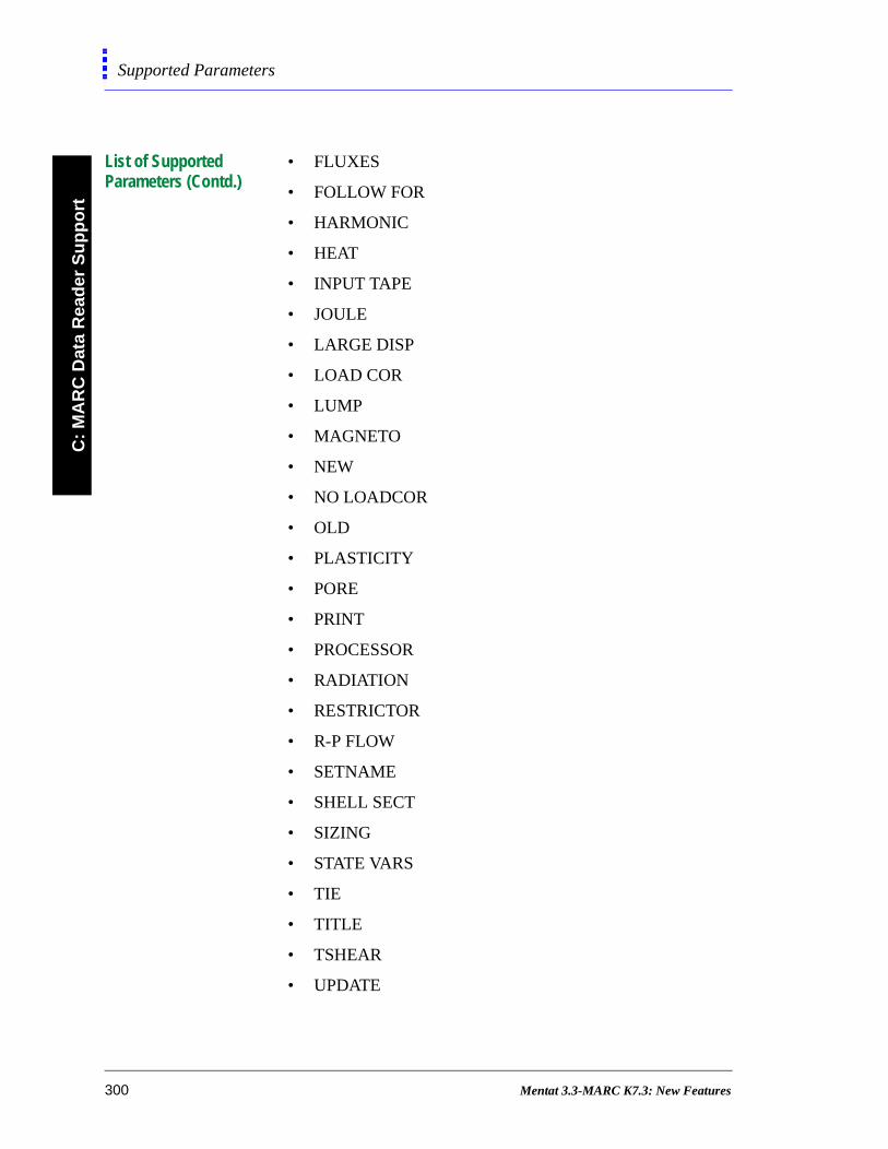
C:
MA
RC
Dat
a R
ead
er S
up
po
rtSupported Parameters
List of Supported Parameters (Contd.)
• FLUXES
• FOLLOW FOR
• HARMONIC
• HEAT
• INPUT TAPE
• JOULE
• LARGE DISP
• LOAD COR
• LUMP
• MAGNETO
• NEW
• NO LOADCOR
• OLD
• PLASTICITY
• PORE
• PROCESSOR
• RADIATION
• RESTRICTOR
• R-P FLOW
• SETNAME
• SHELL SECT
• SIZING
• STATE VARS
• TIE
• TITLE
• TSHEAR
• UPDATE
300 Mentat 3.3-MARC K7.3: New Features
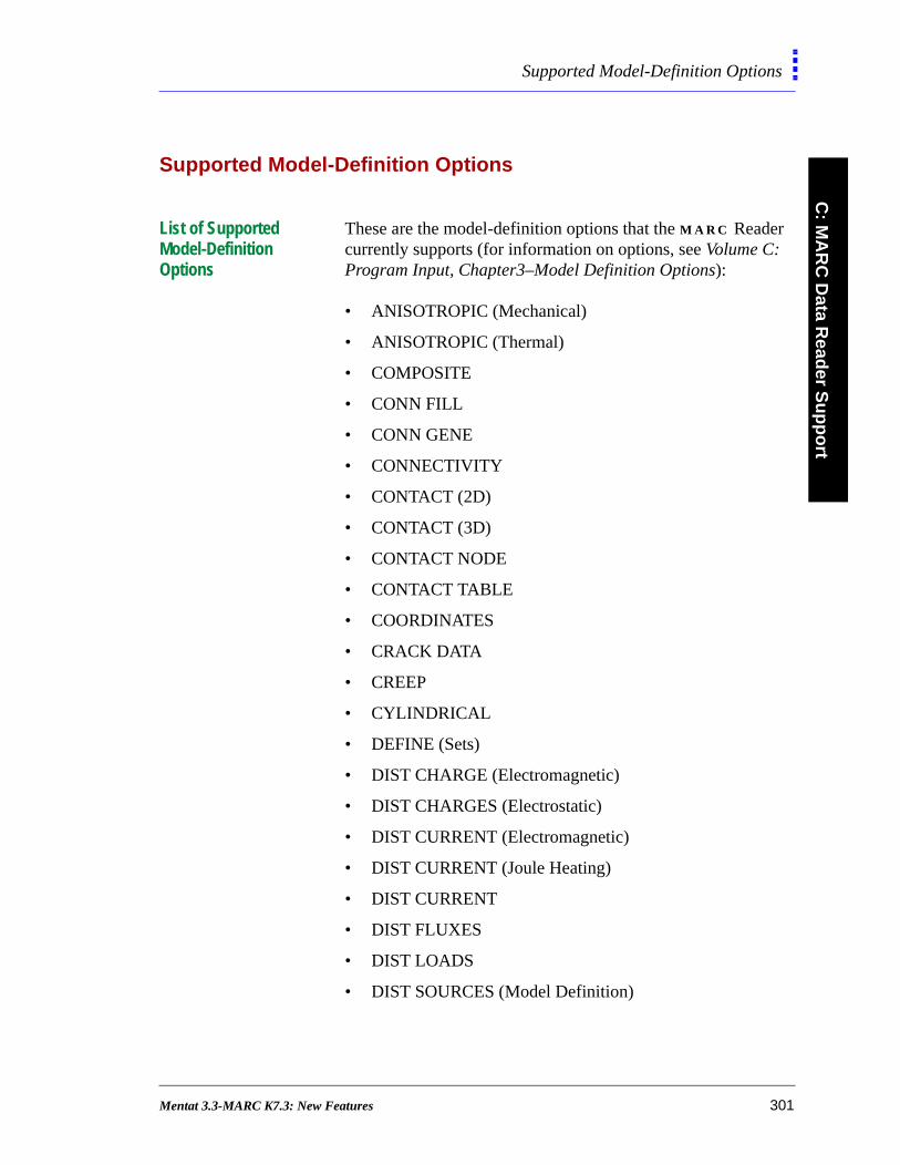
C: M
AR
C D
ata Read
er Su
pp
ort
Supported Model-Definition Options
Supported Model-Definition Options
List of Supported Model-Definition Options
These are the model-definition options that the M A R C Reader currently supports (for information on options, see Volume C: Program Input, Chapter3–Model Definition Options):
• ANISOTROPIC (Mechanical)
• ANISOTROPIC (Thermal)
• COMPOSITE
• CONN FILL
• CONN GENE
• CONNECTIVITY
• CONTACT (2D)
• CONTACT (3D)
• CONTACT NODE
• CONTACT TABLE
• COORDINATES
• CRACK DATA
• CREEP
• CYLINDRICAL
• DEFINE (Sets)
• DIST CHARGE (Electromagnetic)
• DIST CHARGES (Electrostatic)
• DIST CURRENT (Electromagnetic)
• DIST CURRENT (Joule Heating)
• DIST CURRENT
• DIST FLUXES
• DIST LOADS
• DIST SOURCES (Model Definition)
Mentat 3.3-MARC K7.3: New Features 301
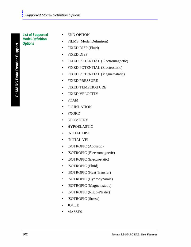
C:
MA
RC
Dat
a R
ead
er S
up
po
rtSupported Model-Definition Options
List of Supported Model-Definition Options
• END OPTION
• FILMS (Model Definition)
• FIXED DISP (Fluid)
• FIXED DISP
• FIXED POTENTIAL (Electromagnetic)
• FIXED POTENTIAL (Electrostatic)
• FIXED POTENTIAL (Magnetostatic)
• FIXED PRESSURE
• FIXED TEMPERATURE
• FIXED VELOCITY
• FOAM
• FOUNDATION
• FXORD
• GEOMETRY
• HYPOELASTIC
• INITIAL DISP
• INITIAL VEL
• ISOTROPIC (Acoustic)
• ISOTROPIC (Electromagnetic)
• ISOTROPIC (Electrostatic)
• ISOTROPIC (Fluid)
• ISOTROPIC (Heat Transfer)
• ISOTROPIC (Hydrodynamic)
• ISOTROPIC (Magnetostatic)
• ISOTROPIC (Rigid-Plastic)
• ISOTROPIC (Stress)
• JOULE
• MASSES
302 Mentat 3.3-MARC K7.3: New Features
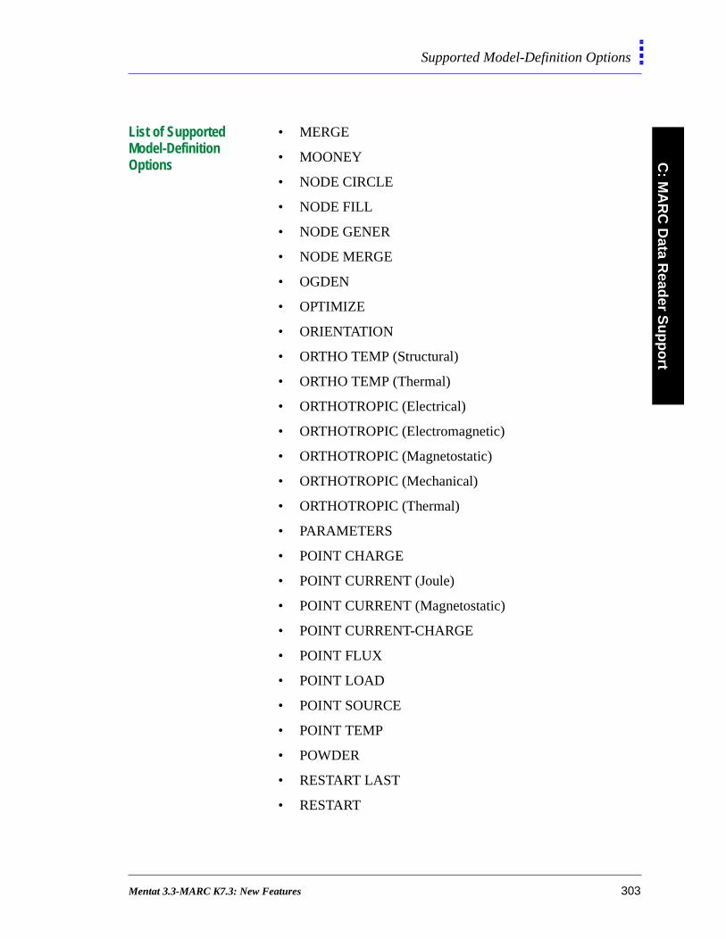
C: M
AR
C D
ata Read
er Su
pp
ort
Supported Model-Definition Options
List of Supported Model-Definition Options
• MERGE
• MOONEY
• NODE CIRCLE
• NODE FILL
• NODE GENER
• NODE MERGE
• OGDEN
• OPTIMIZE
• ORIENTATION
• ORTHO TEMP (Structural)
• ORTHO TEMP (Thermal)
• ORTHOTROPIC (Electrical)
• ORTHOTROPIC (Electromagnetic)
• ORTHOTROPIC (Magnetostatic)
• ORTHOTROPIC (Mechanical)
• ORTHOTROPIC (Thermal)
• PARAMETERS
• POINT CHARGE
• POINT CURRENT (Joule)
• POINT CURRENT (Magnetostatic)
• POINT CURRENT-CHARGE
• POINT FLUX
• POINT LOAD
• POINT SOURCE
• POINT TEMP
• POWDER
• RESTART LAST
• RESTART
Mentat 3.3-MARC K7.3: New Features 303
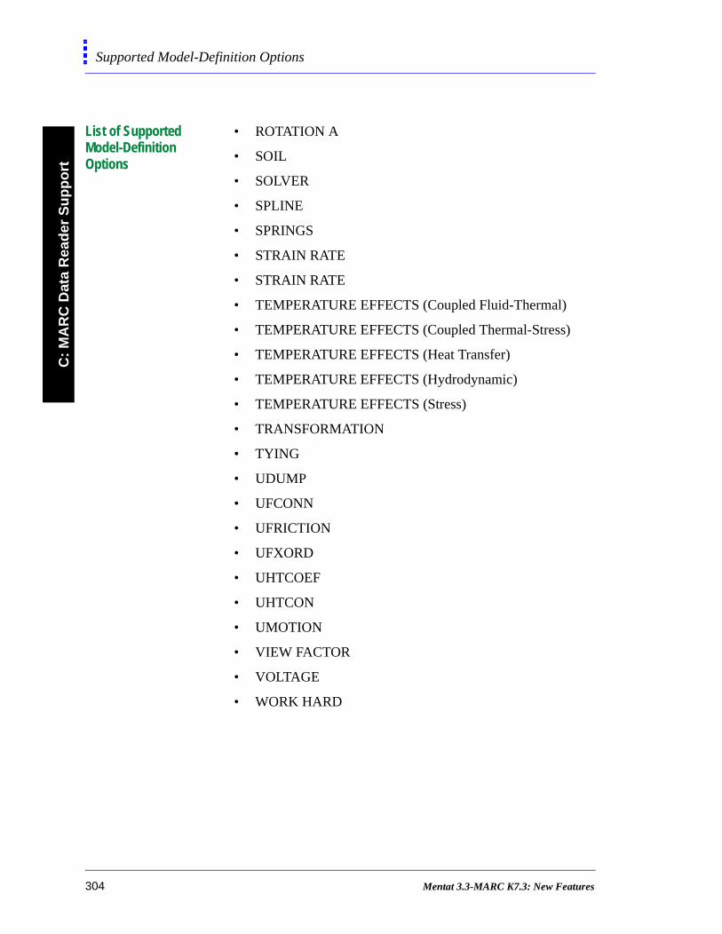
C:
MA
RC
Dat
a R
ead
er S
up
po
rtSupported Model-Definition Options
List of Supported Model-Definition Options
• ROTATION A
• SOIL
• SOLVER
• SPLINE
• SPRINGS
• STRAIN RATE
• STRAIN RATE
• TEMPERATURE EFFECTS (Coupled Fluid-Thermal)
• TEMPERATURE EFFECTS (Coupled Thermal-Stress)
• TEMPERATURE EFFECTS (Heat Transfer)
• TEMPERATURE EFFECTS (Hydrodynamic)
• TEMPERATURE EFFECTS (Stress)
• TRANSFORMATION
• TYING
• UDUMP
• UFCONN
• UFRICTION
• UFXORD
• UHTCOEF
• UHTCON
• UMOTION
• VIEW FACTOR
• VOLTAGE
• WORK HARD
304 Mentat 3.3-MARC K7.3: New Features
D: NASTRAN Writer Data Entries
NASTRAN Writer Bulk Data Entries
The NASTRAN bulk data file export writes the following bulk data entries from the current Mentat database. The data apply to structural analyses only.
Minimum File Requirements 307Bulk Data Cards Written by Mentat 3.3 308Node Coordinates / Transformations 309Material ID’s Included in NASTRAN Geometry Cards 310Loads and Boundary Conditions 312Sample NASTRAN Bulk Data File 313
Mentat 3.3-MARC K7.3: New Features 305

• NASTRAN Writer Bulk Data Entries
Mentat 3.3-MARC K7.3: New Features

D: N
AS
TR
AN
Writer D
ata En
triesMinimum File Requirements
Minimum File Requirements
Minimum File Requirements
Use the following table to determine the positions and corresponding valid entries for data files:
Position Valid Entry
At the start of the bulk data BEGIN BULK
At the end of the bulk data END DATA
Mentat 3.3-MARC K7.3: New Features 307
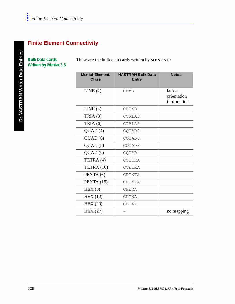
D:
NA
ST
RA
N W
rite
r D
ata
En
trie
sFinite Element Connectivity
Finite Element Connectivity
Bulk Data Cards Written by Mentat 3.3
These are the bulk data cards written by M E N T A T :
Mentat Element/Class
NASTRAN Bulk Data Entry
Notes
LINE (2) CBAR lacks orientation information
LINE (3) CBEND
TRIA (3) CTRLA3
TRIA (6) CTRLA6
QUAD (4) CQUAD4
QUAD (6) CQUAD6
QUAD (8) CQUAD8
QUAD (9) CQUAD
TETRA (4) CTETRA
TETRA (10) CTETRA
PENTA (6) CPENTA
PENTA (15) CPENTA
HEX (8) CHEXA
HEX (12) CHEXA
HEX (20) CHEXA
HEX (27) – no mapping
308 Mentat 3.3-MARC K7.3: New Features
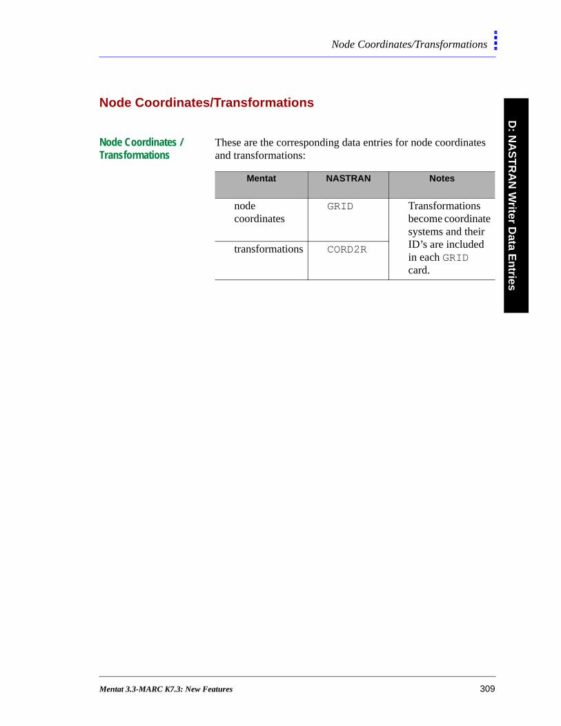
D: N
AS
TR
AN
Writer D
ata En
triesNode Coordinates/Transformations
Node Coordinates/Transformations
Node Coordinates / Transformations
These are the corresponding data entries for node coordinates and transformations:
Mentat NASTRAN Notes
node coordinates
GRID Transformationsbecome coordinate systems and their ID’s are included in each GRID card.
transformations CORD2R
Mentat 3.3-MARC K7.3: New Features 309
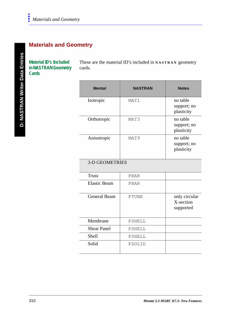
D:
NA
ST
RA
N W
rite
r D
ata
En
trie
sMaterials and Geometry
Materials and Geometry
Material ID’s Included in NASTRAN Geometry Cards
These are the material ID’s included in N A S T R A N geometry cards.
Mentat NASTRAN Notes
Isotropic MAT1 no table support; no plasticity
Orthotropic MAT3 no table support; no plasticity
Anisotropic MAT9 no table support; no plasticity
3-D GEOMETRIES
Truss PBAR
Elastic Beam PBAR
General Beam PTUBE only circular X-section supported
Membrane PSHELL
Shear Panel PSHELL
Shell PSHELL
Solid PSOLID
310 Mentat 3.3-MARC K7.3: New Features
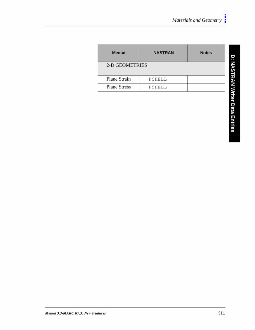
D: N
AS
TR
AN
Writer D
ata En
triesMaterials and Geometry
2-D GEOMETRIES
Plane Strain PSHELL
Plane Stress PSHELL
Mentat NASTRAN Notes
Mentat 3.3-MARC K7.3: New Features 311

D:
NA
ST
RA
N W
rite
r D
ata
En
trie
sLoads and Boundary Conditions
Loads and Boundary Conditions
Loads and Boundary Conditions
These are the corresponding NASTRAN data entries for loads and boundary conditions:
Mentat NASTRAN Notes
FIXED DISPLACEMENT
SPC one card written per degree of freedom
POINT LOAD FORCE
POINT LOAD MOMENT
EDGE LOAD PLOAD1 one card written per component (for beams only)
FACE LOAD PLOAD only normal pressures written
GRAVITY LOAD GRAV
312 Mentat 3.3-MARC K7.3: New Features

D: N
AS
TR
AN
Writer D
ata En
triesSample File
Sample File
Sample NASTRAN Bulk Data File
$$ NASTRAN Bulk Data File created by Mentat II==================================$BEGIN BULK$$ ELEMENT CONNECTIVITY=========================================================$CTETRA 12 8 126 127 125 117$$ TRANSFORMATIONS==============================================================$CORD2R* 1 0 -2.200000 0.000000* -4.400000 -2.200000 4.919350 -4.400000* -2.200000 0.000000 -9.319350$$ NODAL COORDINATES============================================================$GRID* 10 -1.400000 -1.400000* 0.0000000GRID* 20 -0.200000 -2.000000* 0.0000000GRID* 117 -2.200000 -1.000000* -3.2000000GRID* 125 -2.200000 0.000000* -4.4000001GRID* 126 -2.200000 -1.000000* -4.4000000GRID* 127 -1.300000 -1.000000* -4.4000000$$ MATERIALS====================================================================$MAT1* 1 29.000000 0.300000* 1.000000 0.000000$$ GEOMETRY=====================================================================$PSOLID* 8 1*$$ BOUNDARY CONDITIONS==========================================================$FORCE* 1 125 0 1.000000* 10.000000 10.000000 0.000000MOMENT* 1 125 0 1.000000* 20.000000 0.000000 0.000000PLOAD* 4 10.000000117 125* 127GRAV* 5 0 1.000000 0.320000* 0.100000 0.100000$$ SERVO========================================================================$MPC 4 10 1 1.00020 0 0.001ENDDATA
Mentat 3.3-MARC K7.3: New Features 313

Mentat 3.3-MARC K7.3: New Features
E: Command Line Parameters
Mentat 3.3 Command Line Parameters
Table of Additional Command Line Parameters 317
MARC K7.3 Command Line Parameters
Table of MARC K7.3 Command Line Parameters 319
Mentat 3.3-MARC K7.3: New Features 315

• Command Line Parameters
Mentat 3.3-MARC K7.3: New Features
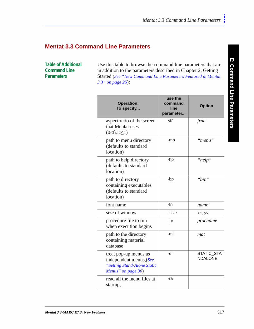
E: C
om
man
d L
ine P
arameters
Mentat 3.3 Command Line Parameters
t
Mentat 3.3 Command Line Parameters
Table of Additional Command Line Parameters
Use this table to browse the command line parameters that are in addition to the parameters described in Chapter 2, Getting Started (See “New Command Line Parameters Featured in Menta3.3” on page 25):
Operation: To specify...
use the command
line parameter...
Option
aspect ratio of the screen that Mentat uses (0<frac<1)
-ar frac
path to menu directory (defaults to standard location)
-mp “menu”
path to help directory (defaults to standard location)
-hp “help”
path to directory containing executables (defaults to standard location)
-bp “bin”
font name -fn name
size of window -size xs, ys
procedure file to run when execution begins
-pr procname
path to the directory containing material database
-ml mat
treat pop-up menus as independent menus,(See “Setting Stand-Alone Static Menus” on page 30)
-df STATIC_STANDALONE
read all the menu files at startup,
-ra
Mentat 3.3-MARC K7.3: New Features 317
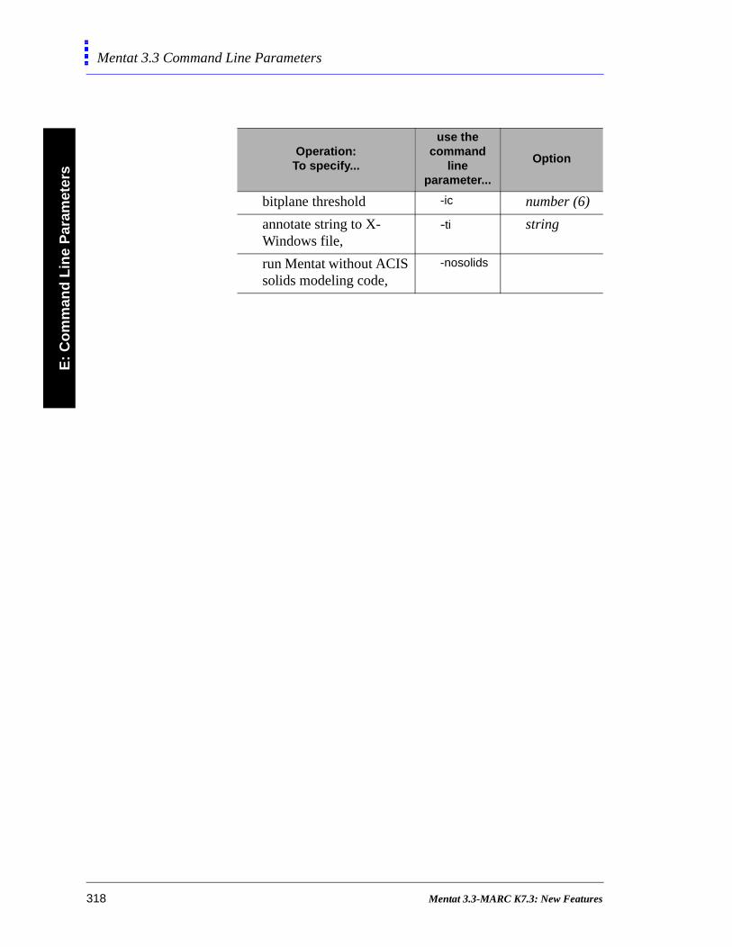
E:
Co
mm
and
Lin
e P
aram
eter
sMentat 3.3 Command Line Parameters
bitplane threshold -ic number (6)
annotate string to X-Windows file,
-ti string
run Mentat without ACIS solids modeling code,
-nosolids
Operation: To specify...
use the command
line parameter...
Option
318 Mentat 3.3-MARC K7.3: New Features

E: C
om
man
d L
ine P
arameters
MARC K7.3 Command Line Parameters
MARC K7.3 Command Line Parameters
Table of MARC K7.3 Command Line Parameters
For a description of the command line parameters in the MARC K7.3 shell script, refer to the following table:
ParameterPossible Names or
ValuesDescription
-prog marck7 run M A R C with or without user subroutines;Run saved module “progname.marc”
-jid jidname identify job/input file
-rid ridname identify previous job for RESTART.
-pid pidname identify job that created temperature file.
-sid sidname identify database file for substructures.
-user username user subroutine username.f used to generate a new load module.
-back yes (default) run program in background.
no Run program in foreground.
-ver yes (default) verify the input syntax.
no don’t verify the input syntax.
-save yes save the generated or existingmodule.
no (default) don’t save the generated or existing module.
-vf viewname identify viewfactor file.
-def def default input file name.
Mentat 3.3-MARC K7.3: New Features 319

Mentat 3.3-MARC K7.3: New Features

F: Demonstration Problems
Demonstration Problems
Lists of Demonstration Problems in MARC K7.3 323
Mentat 3.3-MARC K7.3: New Features 321

• MARC K7:1–Demonstration Problems
Mentat 3.3-MARC K7.3: New Features

F: D
emo
nstratio
n P
rob
lems
Demonstration Problems
s
Demonstration Problems
Lists of Demonstration Problems in MARC K7.3
This section lists selected demonstration problems for the following options in M A R C :
Constant Dilatation
• e3x21f.dat–Necking of a cylindrical bar in tension
Design Sensitivity
• e10x1a.dat–Design sensitivity of the beam geometric
properties of an alternator mount using element 52
• e10x2a.dat–Design sensitivity of the thickness for plane
stress hole in plate problem
• e10x3a.dat–Design sensitivity of elastic material propertie
for the bending of a plate using element type 21
• e10x4a.dat–Design optimization of the thickness for
Scordelis-Lo roof using element type 75
• e10x5a.dat–Design sensitivity of ply angle lay-up for
simple composite plate
• e10x6a.dat–Design sensitivity of 10 bar truss problem
• e10x7a.dat–Design sensitivity of the beam geometric
properties of an alternator mount using element 14
Design Optimization
• e10x1b.dat–Design optimization of the beam geometric
properties of an alternator mount using element 52
• e10x2b.dat–Design optimization of the thickness for plane
stress hole in plate problem
Mentat 3.3-MARC K7.3: New Features 323
F:
Dem
on
stra
tio
n P
rob
lem
sDemonstration Problems
1
• e10x3b.dat–Design optimization of elastic material
properties for the bending of a plate using element type 2
• e10x4b.dat–Design optimization of the thickness for a
Scordelis-Lo roof
• e10x5b.dat–Design optimization of ply angle lay-up for
simple composite plate
• e10x6b.dat–Design optimization of 10 bar truss problem
• e10x7b.dat–Design optimization of the beam geometric
properties of an alternator mount using element 14
Elasticity
• e7x20.dat–Compression of O-ring using 3-term OGDEN
model
• e7x20b.dat–Compression of O-ring using 3-term OGDEN
model (includes follower force stiffness)
• e7x20c.dat–Compression of O-ring using 3-term OGDEN
model (Adaptive Meshing)
• e7x20d.dat–O-ring, using Updated Lagrange procedure -
element 10
• e7x20e.dat–O-ring, using Updated Lagrange procedure -
element 116
• e7x27.dat–Twist of a tapered rod, using OGDEN in
Updated Lagrange procedure
• e7x28a.dat–Expansion of a cylindrical tube, using OGDEN
in Updated Lagrange element type 10
• e7x28b.dat–Expansion of a cylindrical tube, using OGDEN
in Updated Lagrange element type 116
324 Mentat 3.3-MARC K7.3: New Features
F: D
emo
nstratio
n P
rob
lems
Demonstration Problems
e
-
re
• e7x28c.dat–Expansion of a cylindrical tube, using OGDEN
in Updated Lagrange element type 28
• e7x28d.dat–Expansion of a cylindrical tube, using OGDEN
in Updated Lagrange element type 55
• e7x29b.dat–Hole in a plate, OGDEN in Updated Lagrange
procedure - element type 117
• e7x29_def.dat–Defaults file for problems e7x29a and
e7x29b
• e7x30a.dat–Damage model - using discontinuous model
• e7x30b.dat–Damage model - using continuous model
• e7x31a.dat–Rubber seal problem using Updated Lagrang
procedure
• e7x31b.dat–Rezoning of Rubber seal problem using
Updated Lagrange procedure
• e8x43b.dat–Rubber Seal - ELASTICITY,2, - element 10
• e8x43c.dat–Rubber Seal - ELASTICITY,2, - element 116
Plasticity
• e3x19.dat–Upsetting problem using FeFp procedure
• e3x21a.dat–Necking of a cylindrical bar in tension
• e3x21d.dat–Necking of a cylindrical bar in tension
(Adaptive Meshing)
• e3x21e.dat–Necking of a bar using FeFp procedure
• e3x33.dat–Hole in plate - FeFp model - plane stress
• e3x33b.dat–Hole in plate - FeFp model - plane strain
• e3x34.dat–Cylinder expansion using membrane elements
FeFp model
• e3x35.dat–Cantilever beam - plane strain - FeFp procedu
Mentat 3.3-MARC K7.3: New Features 325
F:
Dem
on
stra
tio
n P
rob
lem
sDemonstration Problems
e
n
g
• e3x36.dat–Hole in plate - brick elements - FeFp procedur
• e3x37a.dat–Elastic Deformation in a closed loop - Jauman
rates
• e3x37b.dat–Elastic Deformation in a closed loop - FeFp
• e3x38a.dat–Verify rotational invariance - tension w/rigid
rotation - FeFp plane stress
• e3x38b.dat–Verify rotational invarience - tension w/rigid
rotation - FeFp plane strain
• e8x12d.dat–Bolt forging - FeFp - AUTO STEP, no rezonin
• e8x12dr.dat–Bolt forging - FeFp - AUTO STEP, restart of
e8x12d.dat - Rezoning
• e8x12e.dat–Bolt forging - FeFp - AUTO STEP - Adaptive
• e8x15d.dat–Double-sided contact - FeFp - AUTO STEP
• e8x16b.dat–Hook with release - FeFp - AUTO STEP -
Release (Gradual method)
• e8x17b.dat–Extrusion - FeFp - AUTO STEP
• e8x18c.dat–3-D Forming of a circular blank using
membrane elements - FeFp model
• e8x19b.dat–Indentation rolling - FeFp
• e8x60.dat–Plane strain Brake Forming
Extended
• e8x45.dat–Test of SPLINE option and EXTENDED -
concentric cylinders
• e8x46.dat–Test of EXCLUDE - simple problem
Buckle (Lanczos)
• e3x16b.dat–Plastic buckling using Lanczos procedure
• e4x1d.dat–Shell buckling using Lanczos procedure
326 Mentat 3.3-MARC K7.3: New Features
F: D
emo
nstratio
n P
rob
lems
Demonstration Problems
s
1
• e4x4b.dat–Buckling of a cylindrical tube using Lanczos
procedure
• e4x9b.dat–Non-symmetric buckling of a ring using Lanczo
procedure
• e4x10b.dat–Nonsymmetric buckling of a cylinder using
Lanczos procedure
• e4x15.dat–Buckling of a cylinder tube using Lanczos
procedure
Design Displacement Constraints
• e10x1a.dat–Design sensitivity of the beam geometric
properties of an alternator mount using element 52
• e10x1b.dat–Design optimization of the beam geometric
properties of an alternator mount using element 52
• e10x3b.dat–Design optimization of elastic material
properties for the bending of a plate using element type 2
• e10x5a.dat–Design sensitivity of ply angle lay-up for
simple composite plate
• e10x5b.dat–Design optimization of ply angle lay-up for
simple composite plate
• e10x7a.dat–Design sensitivity of the beam geometric
properties of an alternator mount using element 14
• e10x7b.dat–Design optimization of the beam geometric
properties of an alternator mount using element 14
Design Frequency Constraints
• e10x1a.dat–Design sensitivity of the beam geometric
properties of an alternator mount using element 52
Mentat 3.3-MARC K7.3: New Features 327
F:
Dem
on
stra
tio
n P
rob
lem
sDemonstration Problems
s
1
• e10x1b.dat–Design optimization of the beam geometric
properties of an alternator mount using element 52
• e10x3a.dat–Design sensitivity of elastic material propertie
for the bending of a plate using element type 21
• e10x3b.dat–Design optimization of elastic material
properties for the bending of a plate using element type 2
• e10x4a.dat–Design optimization of the thickness for
Scordelis-Lo roof using element type 75
• e10x4b.dat–design optimization of the thickness for a
Scordelis-Lo roof
• e10x7a.dat–Design sensitivity of the beam geometric
properties of an alternator mount using element 14
• e10x7b.dat–Design optimization of the beam geometric
properties of an alternator mount using element 14
Design Strain Constraints
• e10x2a.dat–Design sensitivity of the thickness for plane
stress hole in plate problem
• e10x2b.dat–Design optimization of the thickness for plane
stress hole in plate problem
• e10x5a.dat–Design sensitivity of ply angle lay-up for
simple composite plate
• e10x5b.dat–Design optimization of ply angle lay-up for
simple composite plate
Design Stress Constraints
• e10x7a.dat–Design sensitivity of the beam geometric
properties of an alternator mount using element 14
328 Mentat 3.3-MARC K7.3: New Features
F: D
emo
nstratio
n P
rob
lems
Demonstration Problems
r
P
)
43
• e10x7b.dat–Design optimization of the beam geometric
properties of an alternator mount using element 14
Exclude
• e8x46.dat–Test of EXCLUDE - simple problem
Parameters
• e2x18.dat–Elastic analysis of shell roof with element 22-
quadratic thick shell element
• e3x14a.dat–Pre-bending of a prismatic beam
• e3x23.dat–Shell roof with geometric and material
nonlinearity-element 75 AUTO INCREMENT
• e4x5.dat–Large displacement analysis of pinched cylinde
• e7x3.dat–Shell roof with material nonlinearity (cracking)-
element 75
• e8x18.dat–Sheet forming of a circular blank with Coulomb
friction
• e8x18d–3-D Forming of a circular blank using AUTO STE
• e9x7a.dat–Natural convection in a square cavity (Ra:1000
• e9x7b.dat–Natural convection in a square cavity
(Ra:10,000)
• e9x7c.dat–Natural convection in a square cavity
(Ra:100,000)
Rebar
• e2x37b.dat–Reinforced concrete beam - elements 11 & 1
• e4x13a.dat–Test of rebar elements type 142
• e4x13b.dat–Test of rebar elements type 144
• e4x13c.dat–Test of rebar elements type 145
Mentat 3.3-MARC K7.3: New Features 329

F:
Dem
on
stra
tio
n P
rob
lem
sDemonstration Problems
• e4x14a.dat–Analysis of a thin cylinder with ply- element 18
& 147
• e4x14b.dat–Analysis of a thin cylinder with plys - element
30 & 148
Region
• e9x10a.dat–Fluid-solid - mixed approach
• e9x10b.dat–Fluid-solid - penalty approach
• e9x10c.dat–Fluid-thermal-solid - mixed approach
• e9x10d.dat–Fluid-thermal-solid - penalty approach
• e9x11a.dat–Fluid flow over a deformable cylinder
• e9x11b.dat–Transient analysis of fluid flow over a
deformable cylinder
• e9x12c.dat–Fluid flow over a deformable cartridge and
thermal effects
• e9x13a.dat–Fluid flow in a deformable tube
• e9x13b.dat–Fluid flow in a deformable tube
Spline
• e8x45.dat–Test of SPLINE option and EXTENDED -
concentric cylinders
Viewfactors
• e5x15b.dat–Radiation analysis using Mentat calculated
viewfactor file
Viscoelastic Exp.
• e7x32.dat–Structural relaxation of a glass cube
330 Mentat 3.3-MARC K7.3: New Features
F: D
emo
nstratio
n P
rob
lems
Demonstration Problems
P
g
Adaptive (Merge)
• e8x44c.dat–Rolling example with ADAPTIVE, allow
element merging
Damage
• e7x30a.dat–Damage model - using discontinuous model
• e7x30b.dat–Damage model - using continuous model
Hypoelastic (HYPELA2)
• e7x29a.dat–Hole in a plate, OGDEN in Updated Lagrange
procedure - element type 7
Auto Step
• e3x12b.dat–Analysis of creep ring-element 10
• e3x21f.dat–necking of a cylindrical bar in tension
• e3x33.dat–Hole in plate - FeFp model - plane stress
• e4x7c.dat–deep arch analysis
• e5x8e.dat–Nonlinear heat conduction with AUTO STEP
• e7x3b.dat–Nonlinear heat conduction without AUTO STE
• e7x4b.dat–Side pressing of a Rubber Hollow Cylinder usin
• e8x12d.dat–Bolt forging - FeFp - no rezoning
• e8x12e.dat–Bolt forging - FeFp - Adaptive
• e8x13b.dat–Coupled analysis of ring compression
• e8x15d.dat–Double-sided contact - FeFp
• e8x16b.dat–Hook with release - FeFp - Release (Gradual
method)
• e8x17b.dat–Extrusion - FeFp
• e8x18d.dat–Sheet forming with spherical punch
Mentat 3.3-MARC K7.3: New Features 331
F:
Dem
on
stra
tio
n P
rob
lem
sDemonstration Problems
Shell to Shell Contact
• e8x51.dat–Test of shell-shell contact for a spring problem
• e8x51b.dat–Test of shell-shell contact, and no increment
splitting for a spring problem
• e8x52.dat–Test of shell-shell contact - stiff hemisphere -
contacts plate
• e8x53a.dat–Test of shell contact
• e8x53b.dat–Test of shell contact
• e8x54.dat–Test of shell contact
Stick to Shell Contact
• e8x47.dat–Test of stick-slip model - def - rigid
• e8x48.dat–Test of stick-slip model - def-def
• e8x49.dat–Test of stick-slip friction model - rubber problem
• e8x50.dat–Test of stick-slip friction model - upsetting
problem
No Splitting
• e8x15c.dat–Double-sided contact - using no splitting
procedure
Load-Controlled Dies
• e8x55b.dat–Deep drawing of a copper sheet - loads
prescribed
• e8x56b.dat–Pressing of a piece - loads prescribed
New Elements
• e2x72.dat–Scordelis-Lo roof - element 138
• e2x74.dat–Scordelis-Lo roof - element 138
332 Mentat 3.3-MARC K7.3: New Features
F: D
emo
nstratio
n P
rob
lems
Demonstration Problems
43
6
• e2x75.dat–Pinched cylinder - element 138
• e4x2c.dat–Square plate under load - element type 138
• e8x57b.dat–Adaptive meshing of simply supported square
plate with point load element type 138
• e2x73.dat–Scordelis-Lo roof - element 139
• e2x76.dat–Pinched cylinder - element 139
• e4x2d.dat–Square plate under load - element type 139
• e8x57c.dat–Adaptive meshing of simply supported square
plate with point load element type 139
• e2x77.dat–Pinched cylinder - element 140
• e4x2e.dat–Square plate under load - element type 140
• e8x57d.dat–Adaptive meshing of simply supported square
plate with point load-element type 140
• e4x13a.dat–Test of rebar elements type 142
• e2x37b.dat–Reinforced concrete beam - elements 11 & 1
• e4x13b.dat–Test of rebar elements type 144
• e4x13c.dat–Test of rebar elements type 145
• e2x14b.dat–Reinforced concrete beam - elements 7 & 14
• e4x14a.dat–Analysis of a thin cylinder with plys - element
18 & 147
• e4x14b.dat–Analysis of a thin cylinder with plys - element
30 & 148
Mentat 3.3-MARC K7.3: New Features 333

Mentat 3.3-MARC K7.3: New Features

Index
Aabsolute distance value. See curvature-dependent di-
visionsabsolute temperature shift 248absolute tolerance
application of 53when to use 53see also adaptive plotting
absolute valuefor design constraints 183see also algebraic value
absorbing role, in heat transfer analysis 279ACIS
binary files 43text files 43see also Import-Export utility
activatingconstant dilatation 100extended precision input 98
activation energy/gas constant (H/R) 247Adaptive Load Stepping procedure 92–97
about 92associated loadcase types 92general parameters for 93
adaptive plotting 52–56changing default settings 55default settings 55default tolerance settings 52pre-defined settings 56safety features 54
added vertex 117adding file extensions. See filter button 41additive decomposition 251Advancing Front mesher 129
checklist for 128
quad mesh 129quad/tri mesh 129tri mesh 129
algebraic value, putting a design constraint on 183allowable distortion, of quadrilateral elements. See
distortion parametersAllowed procedure, for increment splitting 164all-quad mesh 130Analytical Desc. Discontinuity option 147analytical description, of a deformable body 146annotate, string to X-Windows file 318appendixes, about 17applying
fixed divisions to curves 123restrictions to individual curves 125
ar command line parameter 317arrow settings 68–70
specifying arrow attributes 68aspect ratio of the screen, command line parameter
317associating elements with stress or strain constraints
186ASSUMED parameter 103Assumed Strain formulation 102–103
activating 103analysis classes 102associated elements 102
AUTO STEP option. See Adaptive Load Stepping procedure
average length, for curves 122averaging, of nodal values 72axisymmetric element types, for fluids 295axisymmetric rebar elements 213axisymmetric shells, specifying thickness for 181axisymmetric with twist elements 213
Mentat 3.3-MARC K7.3: New Features 335
Ind
ex
Bback command line parameter (MARC) 319back surfaces, identifying 144backface polygons, identifying 144backfaces. See backface polygonsbiaxial deformation mode 263Bingham fluid model 235bitplane threshold, specifying as a command line pa-
rameter 318Body Approach parameter 160Bottom Temperature at Infinity parameter, for con-
trolling emission of radiation 279boundary conditions, for fluid analysis 226bounds
for design constraints 182for design variables 178
Box Pick method. See picking nodesbp command line parameter 317breaking curves 118
when to use 126see also matching curves
brick rebar elements 213brown side, of a 3-D rigid surface 144browsing. See file browserbuckle solutions, using Lanczos method 90–91
about 90parameters 90
bulk data entries, for NASTRAN writer. See NAS-TRAN writer
bulk relaxation tests, computing 272
Ccalibrating quasi-static, stress-strain response
curves 261Carreau fluid model 235centrifugal loads 231centroid 71Centroid option, for rigid bodies 149changing the default parameters. See Numerical
Preferences option 104Check Curves option 119
Check Surfaces option 120checklist, for meshers 128choosing a resolution 66cleaning curves and surfaces. See repair geometrycleaning, loops
2-D curve loops 115surface loops 116
clearing curve divisions 127coefficients, of energy relaxation tests 272color codes, in contact analysis 144Color Print button 63command line
description of parameters 26minimum requirements 26submitting an actual job 26
command line parameters 25, 317command/button sequence 18common retained node 75composite design variable
about 177using 179
Constant Dilatation parameter 100–101when to use 100
CONSTANT parameter. See Constant Dilatation parameter
constant strain amplitude, form of experimental data 262
contact 139–170contact analysis
components of 141physical bodies 142separation procedures 141
Contact Areas option, to indicate contact region 156contact bodies, types of 142contact body release, types of 159contact body, choosing a type of 143contact control
in jobs 161user subroutines for 162
contact distance, in contact table 154Contact Heat Transfer Coeff. button 152contact information
applying to jobs 161applying to loadcases 158
336 Mentat 3.3-MARC K7.3: New Features
Ind
ex
Contact Tables option 154contact tolerances 163continuous contour lines 72Continuous Damage model
about 268checklist for 269
control tolerances, for coupled analysis 241controlling load steps. See Adaptive Load Stepping
procedurecontrolling the emission of radiation, boundary con-
ditions for 278conventions, in this guide 18convergence testing parameters, for solid region in
coupled analysis 242Coons patches 147correcting orientation of contact bodies 145cost, minimizing. See design objectiveCoulomb friction model 167Coulomb-for-Rolling friction model 167coupled analysis 100coupled analysis considerations, for fluid analysis
233coupled analysis, using rigid surfaces 152creating a view snapshot 57curvature-dependent divisions
applying 124benefits of 123
curve divisions 122–128curvature-dependent 123defaults 127fixed average length 123menu 122types of 122
curve facetting. See adaptive plotting, default set-tings
curve geometry, checking 119curve intersection, setting tolerance values for 120curve, expanding elements along 136curves
breaking 118modifying 117splitting 117
curves, drawn and actual. See Adaptive Plotting fea-ture
cusp points 117
Ddamage models
considerations for data sets 269setting control parameters 268
dashpotvalues 76see also springs/dashpots
data types. See Import-Export utilitydef command line parameter (MARC) 319define contact bodies 141defining nodal vectors. See user-defined post vari-
ablesdeformable bodies
analysis parameters 145discrete and analytical descriptions 146meshing 145
deformation mode, form of experimental data 262Delaunay mesher
about 133advantages of 133using 133
deleting file extensions. See filter button.density
of mesh 133design constraints 173, 182–193
applying to related loadcases 176types of 182
design objective 173design optimization
applications of 174components of 173
design sensitivity and optimization 173–206design variables 173, 177–181
linking and unlinking 177picking 177types of 177
detected loops 125determining contact tolerances 141determining number of segments 54df command line parameter 317
Mentat 3.3-MARC K7.3: New Features 337
Ind
ex
Direct Profile solver. See solver optionsDirect Substitution procedure, for solution control
241directed
relative rotation 184relative translation 185rotation 184translation 184
direction cosines. See vector directiondirectories. See file browser.discontinuous contour lines 72Discontinuous Damage model 268discrete description, of a deformable body 146Discrete Kirchoff theory. See Element 138displacement design constraints
about 182removing from a node 184
displayingchanges to files 41directories or files 41
distance tolerance bias value 163distortion parameters
about 130all-tri mesh 130practical values for 130range of values 130specifying 130
documentationadditional MARC K7.1 documents 21online 21online help 20printed 20
dots per inch (dpi) 64double elements with nodes, associating 215DXF
entity summary 45options 45, 47summary reports 45version number 45see also Import-Export utility
dynamic viewing 33rotating a view 34translating a view 34using the Alt key (for UNIX systems only) 33
zooming a view in 34
Eedge loads 229edge radiation, menu 279edge segment length. See curvature-dependent divi-
sionseigenfrequency analysis. See design constraintseigenfrequency design constraints 182eigenvalue constraints
setting 187types of 187units of frequency 187
elastic data, considerations for 252elastomer analysis. See experimental data fittingelement extrapolation 71–72
components of 71methods 71options 72
element typesnew in MARC 290see also fluid element types 290
elementsadding or removing, for stress or strain
constraints 186see also new shell elements
elements, associating with a 3-D membrane or shell 211
emitting roles, in heat transfer analysis 279energy relaxation tests, coefficients for 272enhancements
MARC K7.1 15Mentat 3.1 15
entity 177entity summary, for VDAFS 49Environment Sink Temperature button 152equispaced, forms of data 262Exclude Segments option 157expanding elements along a curve 135–137experimental data fitting 260–273
about 260applying material coefficients 266
338 Mentat 3.3-MARC K7.3: New Features
Ind
ex
damage models 268deciding on a mode 266determining the material coefficients 265experimental tests 261forms of data 262reading in experimental data 261viscoelasticity model 270
EXTENDED parameter. See extended precision in-put
extended precision input 98–99about 98activating 98format changes 99
extrapolating, integration point values 71Extrapolation feature, for experimental data fitting
267
Fface loads 230facets, of arrows 69FIDAP. See Import-Export utilityfile browser 39–41
about 39buttons 41operations 39
filesname and location of 40pathname of 40selecting 40
filter button 41fixed 123fixed divisions for curves 122Fixed Velocity option 226flipping elements, curves and surfaces 145fluid analysis 217–243
about 221boundary conditions 226initial conditions 232loadcases for 238material properties for 234options 222
types of 221fluid element types 225, 295–296fluid models. See viscosity modelsfluid properties, assigning 235fn command line parameter 317font name, specifying as a command line parameter
317font size, increasing 66FORCDT user subroutine 227forcing, even or odd divisions 125format changes. See extended precision inputfraction parameter 248free curves, removing 114Frequency Difference feature 187Friction Coefficient option 145friction coefficient, in contact bodies 154friction model, specifying for contact 142friction models
about 166types of 166
Full Newton-Raphson procedure, for solution con-trol 241
Ggaps in loops. See cleaning loopsgeneralized plane-strain rebar elements 212Generalized Power Law fluid model 235generating, meshes 109geometry
adding or removing 114checking 119summary information 119
geometry design variable 177types of 180using 181
GIF 57glass transition temperature (Tg) 247glass-type materials. See Narayanaswamy modelGradual option, for removing forces 159gravity loads 231Gray button. See PostScript plotting attributesgrayscale, run Mentat in 25
Mentat 3.3-MARC K7.3: New Features 339

Ind
ex
guidelinesfor 2-D and surface meshers 128
guidelines, for loops 128
HHardware Sparse solver. See solver optionshelp directory, specifying path to 317high setting. See adaptive plotting, pre-defined set-
tingshigher ID, of a contacting body 165history definitions, new in MARC 290hollow cross-section 180hollow elements, with uniaxial stiffness. See rebar
elementshourglass stiffness matrix. See Element 140 210hp command line parameter 317HYPELA and HYPELA2, about 257hypoelastic properties, user subroutines for 257
Iic command line parameter 318ID Contact button 144I-DEAS. See Import-Export utilityidentify (MARC command line parameter)
database file for substructures 319job that created temperature file 319job/input file 319previous job for RESTART 319viewfactor file 319
IGESsummary report 47see also Import-Export utility
IGES input filegetting a color 47space curves 47specify a tolerance 47version number 47
image filesetting attributes 63
image filesprinting 62
Image Postscript menu. See PostScript plotting at-tributes
Import-Export utility 42–50export feature 43import feature 42
importing a MARC data file 51incident surfaces 277increasing font size 66increasing strain amplitude, form of experimental
data 262increment splitting options 164individual curves, applying restrictions to 125individual modes, prescribing frequencies for 187initial conditions, for fluid analysis 232Initial Velocity option 150input geometry considerations 127input/output (I/O). See file browser operationsintegration point values 71inter-element averaging. See nodal averaginginterface closure distance, in contact bodies 154interior side
for 2-D contact analysis 144for 3-D contact analysis 144
intersecting loops 120IRIS RGB 57isolate, an element 71Iterative procedure, for increment splitting 164iterative procedures, for solution control 241
Jjid command line parameter (MARC) 319jobs, contact control in 161JPEG 57
changing default attributes 60creating view snapshot file 59default attributes 60Quality button 60setting file attributes 59Smoothing button 60
340 Mentat 3.3-MARC K7.3: New Features
Ind
ex
KKachanov Factor coefficients, computing 268
LLanczos method. See buckle solutions, using Lanc-
zos methodlarge-strain formulation 252layer thickness 180length, for preprocessing arrows 68limitations, on large displacements of solids 233linking design variables 177links 75–85
multiple springs 76resetting program parameters 84types 75UFORMS subroutine 85
listing elements with a 3-D membrane/shell ele-ments 211
load stepping criteriaabout 94for element information 94for nodal values 94settings bounds for 95specifying multiple ranges for 96types of 94
load, as rigid body motion control 151Loadcase option, for contact analysis 158loadcases, for fluids 238log file, creating 25lower ID, of a contacting body 165Lumped Mass method 222
MMARC Data Reader support 297
model-definition options 301parameters 299
MARC Input. See Import-Export utilitymatching curves
about 126
when to use 126see also breaking curves
material design variable 177material mass, minimizing. See design objectivematerial properties, for fluid analysis 234maximum depth. See adaptive plotting safety fea-
turesMean-Normal procedure, for plasticity modeling
251membrane rebar elements 213Mentat entity summary. See DXF optionsmenu files, read at startup. See command line pa-
rametersmenu system
enhancements 28resizing windows 29stand-alone static menus 30window parenting 31
mesh generation 109–134mesh, projecting in the direction of a curve 135meshers
Advancing Front 129Delaunay 133
minimum depth. See adaptive plotting safety fea-tures
missing surfaces. See trimming surfacesMixed method 222mixing formats. See extended precision inputml command line parameter 317Modal Frequency feature 187mode, for all arrows 68model definitions, new in MARC 289modes, prescribing separations between 187modifying, curves 117Monte Carlo method, of viewfactor computation
277Mooney-Rivlin formulations
about 255considerations for 255
motion control, of rigid bodies 149MOTION subroutine. See user subroutines, for con-
tact controlmp command line parameter 317MS-Windows BMP 57multiple springs. See links 75
Mentat 3.3-MARC K7.3: New Features 341
Ind
ex
multiple ties 76multiplicative decomposition 251
NN to 1 option 75N to N option 75Narayanaswamy model 247–250
applying model parameters 248mechanical material types 247parameters for 247
NASTRAN writer, bulk data entries 305bulk data cards 308finite element connectivity 308geometry cards 310loads and boundary conditions 312material ID’s 310minimum file requirements 307node coordinates and transformations 309sample bulk data file 313
NASTRAN. See Import-Export utilitynegative side, setting bounds on 183new enhancements, in MARC
element types 290history definitions 290model definitions 289parameters 289user subroutines 290
new shell elements 209–211Element 138 209Element 139 210Element 140 210
new stress or strain constraints, setting 186Newtonian fluid model 235Next button, using to ignore separation 166nodal averaging 72Nodal Force method, usage 167Nodal Stress method, usage 167nodal ties 76node at midpoint, creating 138node lists 80, 86–89
indicating end of list 86
node ID’s 87specifying 86
node number, associated with the rigid surface 151node path 86–89
picking 88specifying 88storing 89
nodes, excluding 157non-equispaced data set 269normal stress on a plane 185nosolids command line parameter 318Numerical Preferences option 104–105
about 104associated analysis classes 104
NURB description. See rigid bodies, description
Oobjective. See design objectiveOgden formulations
about 255considerations for 255
open loop 120OpenGL graphic system, using. See command line
parametersoperations
for cleaning loops 115for geometry repair 113
optimization. See design sensitivity and optimiza-tion
PPage Height button. See PostScript plotting at-
tributesPage Width button. See PostScript plotting attributesPARAMETER model definition option 105parameters
command line 317parameters, new in MARC 289parenting of windows 31path, specifying as a command line parameter
to directory containing executables 317
342 Mentat 3.3-MARC K7.3: New Features
Ind
ex
to directory containing material database 317to help directory 317to menu directory 317
PATRAN. See Import-Export utilitypenalty function 223Penalty method 222physical bodies, in contact analysis 142picking nodes
box pick 87polygon pick 87
pid command line parameter (MARC) 319planar element types, for fluids 295plane normal, specifying 184plane-strain rebar elements 212plasticity modeling 251–254
element considerations 253types of procedures 251
plotting PostScript image files 62–67ply angle 180, 215point at midpoint, creating 138point loads 228polar decomposition 258Polygon Pick method. See picking nodespop-up menus, treating as independent menus. See
command line parametersposition, as rigid body motion control 151positive side, setting bounds on 183POST model definition option 107post-processing of nodal variables. See user-defined
post variablesPostScript 57
creating the view snapshot file 58plotting attributes 58saving a file 59sending an image file to a printer 59, 63specifying printer destinations 63
Power Law fluid model 235pr command line parameter 317pressure degree of freedom. See Mixed methodpreviously-applied curve divisions, removing 127procedure file 25procedure file to run, specifying as a command line
parameter 317
prog command line parameter (MARC) 319
Rra command line parameter 317Radial Return procedure, for plasticity modeling
251radiation viewfactors 277–284radiation, applying as a boundary condition 278radius, of hollow cross-sections 180ray distribution, for viewfactor computation 278rebar elements 212–216
about 212identifying 213orientation of single strain members 212types of 212
rebar orientation 215relative
rotation about a vector direction 184translation parallel to a vector direction 185
relative tolerance. See adaptive plottingrelaxation spectra 270relaxation table, using 271relaxation, form of experimental data 262releasing nodes in contact 159removing parent attributes. See parenting of win-
dowsrepair geometry 113–121
operations 113Repetitions button 136Report Files button. See VDAFS optionsrescan. See file browserresolution, of PostScript images 64response quantities. See design sensitivity and opti-
mizationretained node per constraint 76retained nodes 75, 76rid command line parameter (MARC) 319rigid bodies
about 148description 152meshing of 148motion control of 149
Mentat 3.3-MARC K7.3: New Features 343

Ind
ex
rigid body 142rigid body, with heat transfer 142root window 29rotating a view. See dynamic viewingRotation Axis option, for rigid bodies 149rotation tensor (R) 258run (MARC command line parameter)
program in background 319program in foreground 319program with or without user subroutines 319
run Mentat, without ACIS solids modeling code. See command line parameters
running MARC 26running Mentat 3.1 25
Ssave command line parameter (MARC) 319save the generated or existing module, MARC com-
mand line parameter. See save command line parameter
scaling, length of arrows. See arrow settingsSDRC model 46segments, excluding. See Exclude Segments optionSel Composite button 180selecting a file. See file browsersensitivity. See design sensitivity and optimizationseparated nodes, preventing re-contact of 159separation force, in contact table 154separation procedures 165separations per increment 166SEPFOR subroutine. See user subroutines, for con-
tact controlSEPSTR subroutine. See user subroutines, for con-
tact controlservo links 76
constraint equation 80using the N to 1 feature with 80using the N to N feature with 81
setting a design space 177setting PostScript image file attributes 63Shear friction model 166shear relaxation tests, computing 272Shear-for-Rolling friction model 166
shell scripts 26sid command line parameter (MARC) 319single-sided contact, using 165size command line parameter 317size of window, specifying as a command line pa-
rameter 317slipping conditions 168small displacements of solid, in fluid analysis 233small-strain formulation 252Snapshot button. See creating a view snapshotsolid arrows 69solution control, of fluid analysis 241solver options 225specific heat matrix, lumping. See Lumped Mass
methodspline, through the nodes 147Split Curves command 117splitting curves 117springs
N to N springs 76springs/dashpots
menus 77using the N to 1 feature with 82using the N to N feature with 83USPRNG subroutine 82
Staggered procedure. See weakly coupledstand-alone static menus 30steady state fluid problem, prescribing final veloci-
ties 227steady state, fluid loadcase type 238step ratio, for adaptive load stepping 94Stick-Slip friction model 167Stick-Slip option
about 168available parameters 168
strain design constraints 182stress design constraints 182stress relaxation table 270stretch tensor(U) 258strongly coupled 222Suppressed procedure, for increment splitting 164surface facetting. See adaptive plotting, default set-
tingssurface geometry, checking 119
344 Mentat 3.3-MARC K7.3: New Features

Ind
ex
surface parametric space 116symmetry bodies 153symmetry planes, in viewfactor computation 281symmetry rigid body 142synchronized approach, in contact analysis 160
TTable Properties feature, in contact tables 154tangential force, at previous iteration 169Temperature at Infinity parameter, for controlling
emission of radiation 278thermal expansion property, in Narayanaswamy
model 249thermo-rheologically simple materials 247three-dimensional element types, for fluids 296ti command line parameter 318tied nodes 76TIFF 57tolerance options, for curvature-dependent curve di-
visions 124tolerance value
for curve intersections 120for intersecting loops 121
tolerance, in adaptive plotting 52topology information. See geometrytouching bodies
about 155selecting 155
transient parameters for fluid analyses, applying 240transient, fluid loadcase type 238translating a view. See dynamic viewingtranslating data types. See Import-Export utilitytri-mesh
shape 133size 133transition 133see also meshers
trimming, surfaces 114tying types 78
UUCONTACT subroutine. See user subroutines, for
contact controlUFRIC subroutine. See user subroutines, for contact
controlUHTCOE subroutine. See user subroutines, for con-
tact controlUHTCON subroutine. See user subroutines, for con-
tact controlundo, box or polygon pick 87UNEWTN user subroutine, for fluid analysis 243uniaxial data, for curve fitting 261uniaxial, deformation mode 263Unlinked button 177Updated Lagrange procedure 255UPOSTV subroutine
activating 106additional information 107
Upper Bound button 178user command line parameter (MARC) 319user enhancements, list of 289–291user subroutines
for contact control 162new in MARC 290
User-Defined fluid model 235user-defined post variables 106–107
Vvalidating IGES entities. See IGES optionsvariables. See design variablesVDAFS
Mentat entity summary 49version number 49see also Import-Export utility
vector direction, specifying 184velocity
as rigid body motion control 150prescribing at nodal points 226
velocity as initial condition, in fluid analysis 233ver command line parameter (MARC) 319verifying the input syntax in MARC, command line
parameter for 319
Mentat 3.3-MARC K7.3: New Features 345
Ind
ex
vertex tolerance 126vf command line parameter (MARC) 319View Snapshot feature 57–60viewfactors
about 277computing 280emitting surfaces 277
viscoelastic materialsthermo-rheologically simple 247
viscoelastic thermal expansion property 249viscosity models 235volume, minimizing. See design objective
Wwall thickness, of hollow cross-sections 180weakly coupled 222window manager attributes 31wireframe arrows 69work-hardening data, considerations for 252
XX-Origin button. See PostScript plotting attributes
YY-Origin button. See PostScript plotting attributes
ZZ-component, for Foam models 263zooming a view in. See dynamic viewing
346 Mentat 3.3-MARC K7.3: New Features
Document Title: Mentat 3.3-MARC K7.3:New FeaturesPart Number: UG-3012-01Revision Date: August, 1998
UNITED STATESCALIFORNIA - Palo AltoMARC Corporate Headquarters260 Sheridan Avenue, Suite 309Palo Alto, CA 94306, USATel: 1 650 329 6800Fax: 1 650 323 5892Email: [email protected]
GERMANY - MunichMARC Software Deutschland GmbHIsmaninger Str. 985609 Aschheim (bie Munich)GermanyTel: 49 (89) 904 50 33Fax: 49 (89) 903 06 76Email: [email protected]
PACIFIC RIMCHINAMARC Overseas, Inc.Bright Chang An Building, Suite 3217# Jian Guo Men Nei StreetBeijing, China 100 005Tel: 86 (10) 6510 2056
86 (10) 6510 205786 (10) 6510 2058
Fax: 86 (10) 6510 2053Email: [email protected]
CALIFORNIA - San DiegoMARC Analysis Research Corp.4330 LaJolla Village Drive, Suite 320San Diego, CA 92122Tel: 1 619 658 9588Fax: 1 619 758 8710
GERMANY - HannoverMARC Software Deutschland GmbHAlte Dohrener Str. 66D 30173 Hannover, GermanyTel: 49 (511) 980 5182Fax: 49 (511) 980 5187
JAPAN - NagoyaNippon MARC Co., Ltd.Nagoya Nishiki Daiichi Seimei Bldg.2F, 6-5 Nishiki 1-chomeNaka-ku, Nagoya, Aichi 460-0003Tel: 81 (52) 202 5661Fax: 81 (52) 202 5665
CONNECTICUT - E. BerlinMARC Analysis Research Corp.1224 Mill StreetE. Berlin, CT 06023Tel: 1 860 828 2055Fax: 1 860 828 2031
ITALYEspri-MARC s.r.l.Viale Brigata Bisagno 2/1016129 Genova, ItalyTel: 39 (10) 585 949Fax: 39 (10) 585 949Email: [email protected]
JAPAN - OsakaNippon MARC Co., Ltd.4F 2nd Kimi Building2-11 Toyotucho Suita-shiOsaka 564-0051Tel: 81 (6) 385 1101Fax: 81 (6) 385 4343
MICHIGAN - Ann ArborMARC Analysis Research Corp.24 Frank Lloyd Wright DriveAnn Arbor, MI 48106-0523Tel: 1 734 998 0540Fax: 1 734 998 0542
THE NETHERLANDSMARC Analysis Research CorporationDublinstraat 322713 HS ZoetermeerThe NetherlandsTel: 31 (79) 3510 411Fax: 31 (79) 3517 560Email: [email protected]
JAPAN - Tokyo(Asian Operations Headquarters)Nippon MARC Co., Ltd.Shinjuku Daiichi Seimei BuildingP.O. Box 50562-7-1 Nishi-Shinjuku, Shinjuku-kuTokyo 163-0704Tel: 81 (3) 3345 0181Fax: 81 (3) 3345 1529Email: [email protected]
EUROPECZECH REPUBLICMARC Overseas, Inc.Podolska 50147 00 Praha 4Czech RepublicTel: 420 (2) 6121 4123
420 (2) 6121 4111 x252Fax: 420 (2) 6121 4123Email: [email protected]
UNITED KINGDOMMARC UK Ltd.11 Linford Forum, Rockingham DriveLinford WoodMilton Keynes, MK14 6LYTel: 44 (1908) 606 070Fax: 44 (1908) 606 633Email: [email protected]
KOREADong Kyung Bldg. 7FL824-19 Yuksam-DongKangnam-Ku, Seoul, KoreaTel: 82 (2) 561 7543Fax: 82 (2) 561 7767Email: [email protected]
FRANCEMARC France S.A.Bercy Expo SR 6101A40 Avenue des Terroirs de France75611 Paris Cedex 12, FranceTel: 33 (1) 4474 1550Fax: 33 (1) 4474 1554Email: [email protected]