Mental Health Sensing Using MachineLearning

A Major Qualifying Project submitted to the faculty ofWorcester Polytechnic Institute in partial fulfillment of the

requirements for the Degree of Bachelor of Science inComputer Science

Joseph Caltabiano, Nicolas Pingal, Myo Min Thant,Yared Taye, Adam Sargent, Yosias Seifu

Advised by Professor Elke A. Rundensteinerand

Professor Randy C. Paffenroth

April 1, 2020

IRB-18-0031

This report represents the work of one or more WPI undergraduate studentssubmitted to the faculty as evidence of completion of a degree requirement.

WPI routinely publishes these reports on its website without editorial orpeer review.

I

Abstract

Using audio and text data from multiple sources, we evaluated theviability of using machine and deep learning to identify depression andanxiety. Machine learning methods using sub-clip boosting achievedan F1 score of 0.81 for depression and 0.83 for anxiety. Our convo-lutional neural networks and long-term short term memory modelsachieved F1 scores of 0.55 and 0.68 respectively for depression. Asfeature engineering, we used topological data analysis to create Betticurves in our machine learning pipeline. Furthermore, we developeda pipeline to generate text messages with deep learning models, fordata augmentation purposes.

II

Acknowledgements

There are a number of others involved with this project that we would liketo thank for making the whole thing possible. First, we would like to thankProfessor Elke Rundensteiner, our project advisor, and our two graduatestudents, ML Tlachac and Ermal Toto, for their continual support and helpduring our project. Ermal in particular, was a huge help with explainingdeep learning and machine learning techniques, managing git repositoriesand Ace cluster and setting up pipelines for us to continue working on eachsub-project systematically, while ML helped us out with the TDA and textgeneration facets of our project, providing some code to help run machinelearning experiments with TDA data in particular. For the math portion ofthe MQP, we would like to thank Professor Randy Paffenroth for advisingand providing support with the finer details of the mathematical writingprocess.

Next, we would like to thank the computer science department of WPI asa whole, for allowing us to use their resources for our experiments. JamesKingsley must be thanked, for helping us to figure out how to configure thenecessary resources to run experiments on the ACE and Turing clusters. Wewouldn’t be able to complete our experiments without being able to run onthe ACE and Turing clusters.

Finally, we would like to thank a few specific individuals. Weili Nie, oneof the head developers of RelGAN, was incredibly helpful while we weretrying to figure out how to run RelGAN with our data set, and we wouldlike to thank him for that. We would also like to thank Meryll Dindin fordevloping the TdaToolbox on github, which served as a basis for our Betticurve generation1.

1https://github.com/Coricos/TdaToolbox

III

Contents

Abstract II

Acknowledgements III

Contents IV

List of Figures VIII

List of Tables XII

1 Introduction 11.1 Related Works . . . . . . . . . . . . . . . . . . . . . . . . . . . 11.2 Our Approach . . . . . . . . . . . . . . . . . . . . . . . . . . . 3

1.2.1 Machine Learning . . . . . . . . . . . . . . . . . . . . . 41.2.2 Convolutional Neural Network . . . . . . . . . . . . . . 41.2.3 Sequential Deep Learning Model . . . . . . . . . . . . . 41.2.4 GANs . . . . . . . . . . . . . . . . . . . . . . . . . . . 51.2.5 Topological Data Analysis . . . . . . . . . . . . . . . . 5

2 Background 62.1 Previous MQPs . . . . . . . . . . . . . . . . . . . . . . . . . . 6

2.1.1 2018 MQP summary . . . . . . . . . . . . . . . . . . . 62.1.2 2019 MQP summary . . . . . . . . . . . . . . . . . . . 6

2.2 Depression Statistics . . . . . . . . . . . . . . . . . . . . . . . 72.2.1 Patient Health Questionnaire . . . . . . . . . . . . . . 72.2.2 General Anxiety Disorder . . . . . . . . . . . . . . . . 8

2.3 Data Sources . . . . . . . . . . . . . . . . . . . . . . . . . . . 82.3.1 DAIC-WOZ . . . . . . . . . . . . . . . . . . . . . . . . 92.3.2 Moodable . . . . . . . . . . . . . . . . . . . . . . . . . 102.3.3 EMU . . . . . . . . . . . . . . . . . . . . . . . . . . . . 11

2.4 Dimensionality Reduction Techniques . . . . . . . . . . . . . . 112.4.1 Principle Component Analysis (PCA) . . . . . . . . . . 122.4.2 Non-Negative Matrix Factorization (NMF) . . . . . . . 12

2.5 Data Balancing . . . . . . . . . . . . . . . . . . . . . . . . . . 132.5.1 Under sampling . . . . . . . . . . . . . . . . . . . . . . 142.5.2 Oversampling . . . . . . . . . . . . . . . . . . . . . . . 142.5.3 Synthetic Minority Oversampling Technique . . . . . . 15

IV

2.6 Evaluation Metrics . . . . . . . . . . . . . . . . . . . . . . . . 152.6.1 Confusion Matrix . . . . . . . . . . . . . . . . . . . . . 152.6.2 Accuracy . . . . . . . . . . . . . . . . . . . . . . . . . 162.6.3 Precision . . . . . . . . . . . . . . . . . . . . . . . . . . 172.6.4 Sensitivity . . . . . . . . . . . . . . . . . . . . . . . . . 172.6.5 Specificity . . . . . . . . . . . . . . . . . . . . . . . . . 172.6.6 F1-Score . . . . . . . . . . . . . . . . . . . . . . . . . . 172.6.7 Area under the ROC Curve (AUC) . . . . . . . . . . . 182.6.8 Mean Squared Error (MSE) . . . . . . . . . . . . . . . 192.6.9 Root Mean Squared Error (RMSE) . . . . . . . . . . . 192.6.10 Mean Absolute Error (MAE) . . . . . . . . . . . . . . 202.6.11 R-Squared . . . . . . . . . . . . . . . . . . . . . . . . . 20

2.7 Machine Learning . . . . . . . . . . . . . . . . . . . . . . . . . 212.7.1 K-Nearest Neighbors . . . . . . . . . . . . . . . . . . . 212.7.2 Support Vector Machines . . . . . . . . . . . . . . . . . 222.7.3 Logistic Regression . . . . . . . . . . . . . . . . . . . . 232.7.4 Artificial Neural Network . . . . . . . . . . . . . . . . . 232.7.5 Random Forest and Decision Trees . . . . . . . . . . . 242.7.6 XGBoost . . . . . . . . . . . . . . . . . . . . . . . . . . 272.7.7 Voting . . . . . . . . . . . . . . . . . . . . . . . . . . . 28

2.8 Deep Learning . . . . . . . . . . . . . . . . . . . . . . . . . . . 292.8.1 Convolutional Neural Network (CNN) . . . . . . . . . 292.8.2 Sequence Modelling: Recurrent Neural Networks (RNN) 312.8.3 Sequence Modelling: Long Short Term Memory (LSTM)

Models and Gated Recurrent Units (GRU) . . . . . . . 332.8.4 Feeding Audio Data into Neural Networks . . . . . . . 35

2.9 Machine Learning and Deep Learning Frameworks . . . . . . . 372.9.1 Pytorch . . . . . . . . . . . . . . . . . . . . . . . . . . 372.9.2 TensorFlow . . . . . . . . . . . . . . . . . . . . . . . . 382.9.3 Keras . . . . . . . . . . . . . . . . . . . . . . . . . . . 38

2.10 Topological Data Analysis . . . . . . . . . . . . . . . . . . . . 392.10.1 Definition . . . . . . . . . . . . . . . . . . . . . . . . . 392.10.2 Simplicial Complex . . . . . . . . . . . . . . . . . . . . 392.10.3 Persistent Homology . . . . . . . . . . . . . . . . . . . 412.10.4 Persistence Barcodes And Persistence Diagram . . . . . 412.10.5 Interpreting Topological Data . . . . . . . . . . . . . . 43

2.11 Generative Adversarial Networks . . . . . . . . . . . . . . . . 442.11.1 Sequence GAN . . . . . . . . . . . . . . . . . . . . . . 44

V

2.11.2 Sequence GAN Variants . . . . . . . . . . . . . . . . . 452.11.3 Sequence GAN Evaluation Metrics . . . . . . . . . . . 47

3 Feature Extraction 483.1 Text Feature Extraction for Machine Learning . . . . . . . . . 483.2 Audio Feature Extraction for Machine Learning . . . . . . . . 48

3.2.1 Pratt . . . . . . . . . . . . . . . . . . . . . . . . . . . . 483.2.2 openSMILE . . . . . . . . . . . . . . . . . . . . . . . . 49

3.3 Topological Data Analysis . . . . . . . . . . . . . . . . . . . . 493.3.1 Constructing Filtered Complex From Sound Waves . . 50

3.4 Generative Adversarial Networks . . . . . . . . . . . . . . . . 55

4 Methods 554.1 Machine Learning . . . . . . . . . . . . . . . . . . . . . . . . . 55

4.1.1 Machine Learning Pipeline . . . . . . . . . . . . . . . . 554.1.2 Machine Learning Method Configurations . . . . . . . 56

4.2 Deep Learning . . . . . . . . . . . . . . . . . . . . . . . . . . . 594.2.1 CNN Experimental Setup . . . . . . . . . . . . . . . . 594.2.2 LSTM Experimental Setup . . . . . . . . . . . . . . . . 604.2.3 Deep Learning Pipelines . . . . . . . . . . . . . . . . . 614.2.4 Experimental Planning . . . . . . . . . . . . . . . . . . 63

4.3 Tests Run on Audio Data . . . . . . . . . . . . . . . . . . . . 684.4 Tests Run on Transcript . . . . . . . . . . . . . . . . . . . . . 68

4.4.1 Tests Run on Audio and Transcript . . . . . . . . . . . 694.5 Topological Data Analysis . . . . . . . . . . . . . . . . . . . . 704.6 Generative Adversarial Networks . . . . . . . . . . . . . . . . 71

4.6.1 ACE Experiments . . . . . . . . . . . . . . . . . . . . . 724.6.2 Turing Experiments . . . . . . . . . . . . . . . . . . . . 74

5 Results 755.1 Machine Learning . . . . . . . . . . . . . . . . . . . . . . . . . 75

5.1.1 GAD-7 Experiments on EMU . . . . . . . . . . . . . . 755.1.2 PHQ-8 Experiments with EMU . . . . . . . . . . . . . 795.1.3 PHQ-8 Experiments with EMU+Moodable . . . . . . . 825.1.4 DAIC-WOZ Audio Experiments . . . . . . . . . . . . . 835.1.5 DAIC-WOZ Transcript+Audio Experiments . . . . . . 875.1.6 Audio vs Transcript + Audio Predictions Analysis . . . 87

5.2 Deep Learning . . . . . . . . . . . . . . . . . . . . . . . . . . . 88

VI

5.2.1 EMU/Moodable: CNN . . . . . . . . . . . . . . . . . . 885.2.2 DAIC-WOZ: CNN . . . . . . . . . . . . . . . . . . . . 895.2.3 DAIC-WOZ: Sequential Model . . . . . . . . . . . . . . 99

5.3 Topological Data Analysis . . . . . . . . . . . . . . . . . . . . 1085.4 Generative Adversarial Networks . . . . . . . . . . . . . . . . 111

5.4.1 ACE Experiments . . . . . . . . . . . . . . . . . . . . . 1115.4.2 Turing Experiments . . . . . . . . . . . . . . . . . . . . 113

6 Conclusion 1156.1 Machine Learning . . . . . . . . . . . . . . . . . . . . . . . . . 1166.2 Deep Learning . . . . . . . . . . . . . . . . . . . . . . . . . . . 1176.3 Topological Data Analysis . . . . . . . . . . . . . . . . . . . . 1196.4 Generative Adversarial Networks . . . . . . . . . . . . . . . . 120

A Tables of Accomplishments 121A.1 A Term . . . . . . . . . . . . . . . . . . . . . . . . . . . . . . 121A.2 B Term . . . . . . . . . . . . . . . . . . . . . . . . . . . . . . 123A.3 C Term . . . . . . . . . . . . . . . . . . . . . . . . . . . . . . 125

B Table of Authorship 127

VII

List of Figures

1 Results of the 2017 Review (Guntuku et al., 2017) . . . . . . . 22 Results of Arrhythmia Study (Dindin et al., 2019) . . . . . . . 53 PHQ-9 Accuracy from 2009 study (Kroenke et al., 2009) . . . 84 Histogram of PHQ-8 scores from AVEC data set (Ringeval

et al., 2017) . . . . . . . . . . . . . . . . . . . . . . . . . . . . 105 PCA on a small data set (Brems, 2019) . . . . . . . . . . . . . 126 NMF on an audio spectrogram (Librosa Development Team,

2019) . . . . . . . . . . . . . . . . . . . . . . . . . . . . . . . . 137 Resampling of data set . . . . . . . . . . . . . . . . . . . . . . 158 Confusion Matrix . . . . . . . . . . . . . . . . . . . . . . . . . 169 F1-Score . . . . . . . . . . . . . . . . . . . . . . . . . . . . . . 1810 AUC-ROC graph . . . . . . . . . . . . . . . . . . . . . . . . . 1811 Mean Square Error Formula . . . . . . . . . . . . . . . . . . . 1912 Root Mean Square Error Formula . . . . . . . . . . . . . . . . 2013 Root Mean Absolute Error Formula . . . . . . . . . . . . . . . 2014 R2 . . . . . . . . . . . . . . . . . . . . . . . . . . . . . . . . . 2115 K Nearest Neighbors Diagram (Ali, 2018) . . . . . . . . . . . . 2216 SVC Diagram (Gandhi, 2018) . . . . . . . . . . . . . . . . . . 2217 Artificial Neural Network Diagram . . . . . . . . . . . . . . . 2418 Simple Decision Tree . . . . . . . . . . . . . . . . . . . . . . . 2519 Random Forest vs Decision Tree . . . . . . . . . . . . . . . . . 2620 Random Forest Classifier . . . . . . . . . . . . . . . . . . . . . 2721 XGBoost Plot of Single Decision Tree . . . . . . . . . . . . . . 2822 Convolutional Neural Network (Saha, 2018) . . . . . . . . . . 2923 Operation of a Convolutional Layer (Saha, 2018) . . . . . . . . 3024 Operation of Max Pooling and Average Pooling Layers (Saha,

2018) . . . . . . . . . . . . . . . . . . . . . . . . . . . . . . . . 3125 Topologies of RNN, LSTM, and GRU (van Veen, 2017) . . . . 3226 An unrolled RNN (Banerjee, 2018) . . . . . . . . . . . . . . . 3227 Inside an LSTM cell (van Veen, 2017) . . . . . . . . . . . . . . 3428 An LSTM cell (Ma et al., 2016) . . . . . . . . . . . . . . . . . 3529 Processing raw audio wave (Mansar, 2018) . . . . . . . . . . . 3630 Processing mel-spectrogram (Mansar, 2018) . . . . . . . . . . 3731 Popularity of three frameworks among researchers (Sayantini,

2019) . . . . . . . . . . . . . . . . . . . . . . . . . . . . . . . . 3932 Example of constructing a simplicial complex (Meryll, 2018) . 40

VIII

33 Example of a Filtered Complex (Bubenik, 2017) . . . . . . . . 4034 Example of a Persistence Barcode of a Filtered Complex. H0

is 0-d holes, as explained in the above paragraph. Multiplesteps of a filtered complex are show, and at each picture thenumber of lines in the barcode is equal to the number of 0-dholes in the shown complex (Ghrist, 2008) . . . . . . . . . . . 41

35 Persistence Diagram of a Filtered Complex Formed from aSound Clip. This particular clip was from the DAIC-WOZdata set (see section 2.3.1. Each point corresponds to thebirth and death date of a feature in the sound clip . . . . . . . 42

36 Example of constructing a Betti curve with 100 componentsfrom a persistence barcode. Unlike Figure 34, the featurestracked have varying birth dates . . . . . . . . . . . . . . . . . 43

37 Diagram of GAN Process (Goodfellow et al., 2014) . . . . . . 4438 Sequence GAN Diagram (Yu et al., 2016) . . . . . . . . . . . . 4539 LeakGAN Flow Diagram (Guo et al., 2017) . . . . . . . . . . . 4640 NLL-Loss (Yu et al., 2016) . . . . . . . . . . . . . . . . . . . . 4741 A Simplicial complex from a simplified sound wave . . . . . . 5042 First Filtration Level of Wave Filtered Complex, X0. Each

segment with a filtration level less than X0 is added . . . . . . 5143 Second Filtration Level of Wave Filtered Complex, X1. Each

segment with a filtration level less than X1 is added . . . . . . 5144 Third Filtration Level of Wave Filtered Complex, X2. Each

segment with a filtration level less than X2 is added . . . . . . 5245 Fourth Filtration Level of Wave Filtered Complex, X3. Each

segment with a filtration level less than X3 is added . . . . . . 5246 Fifth Filtration Level of Wave Filtered Complex, X4. Each

segment with a filtration level less than X4 is added . . . . . . 5347 TDA Feature Extraction Pipeline . . . . . . . . . . . . . . . . 5348 All combinations of method, data set, feature type, goal, and

prediction type in this paper . . . . . . . . . . . . . . . . . . . 5449 Machine Learning Pipeline . . . . . . . . . . . . . . . . . . . . 5650 Convolutional Neural Network pipeline . . . . . . . . . . . . . 6251 Sequence Model (LSTM) pipeline . . . . . . . . . . . . . . . . 6352 Workflow between Image Caching and without Caching . . . . 6453 Combining Convolution and openSMILE . . . . . . . . . . . . 6754 Frequency Graph for Transcript Data (Ali, 2018) . . . . . . . 6855 Histogram of Transcript Data (Ali, 2018) . . . . . . . . . . . . 69

IX

56 Pipeline for Machine Learning Using Betti Curves . . . . . . . 7157 Moodable: Ten Most Frequent Words . . . . . . . . . . . . . . 7258 Moodable: Ten Participants with the Most Texts . . . . . . . 7359 Text Generation Pipeline . . . . . . . . . . . . . . . . . . . . . 7460 Classification: GAD-7 Experiments Top F1 Scores . . . . . . . 7661 Classification: Best Test runs for Cutoff=10 . . . . . . . . . . 7662 Regression: GAD-7 Experiments Top F1 Scores . . . . . . . . 7663 F1 Score distribution across Models . . . . . . . . . . . . . . . 7764 F1 Score distributions among Resampling Techniques . . . . . 7765 F1 Score distributions among Binary Cutoffs . . . . . . . . . . 7866 Predictions for un-split and no-overlap . . . . . . . . . . . . . 7967 Previous MQP EMU dataset experiment results . . . . . . . . 8068 EMU PHQ Experiments Best Results . . . . . . . . . . . . . . 8069 F1 Score distribution across Models . . . . . . . . . . . . . . . 8170 F1 Score distributions among Resampling Techniques . . . . . 8171 F1 Score distributions among Binary Cutoffs . . . . . . . . . . 8272 EMU+Moodable PHQ Experiments Best Results . . . . . . . 8273 F1 Score distributions for EMU+Moodable . . . . . . . . . . . 8374 F1 Score distribution for Participant Grouping . . . . . . . . . 8475 F1 Score distribution for Participant + Question Grouping . . 8576 F1 Score distribution for Participant Grouping . . . . . . . . . 8677 F1 Score distribution for Participant + Question Grouping . . 8678 Best Performers: DAIC-WOZ Audio + Transcript . . . . . . . 8879 Results from running CNN on EMU and Moodable Data . . . 8980 The confusion matrix data for four best performing experiments 9281 Results from running 7x7 convolution and 5x5 max pool . . . 9382 Best Results from running CNN with openSMILE176 . . . . . 9883 A comparison of Adam vs RMSProp with a learning rate of

1e-5, 128 nodes, and 1 layer . . . . . . . . . . . . . . . . . . . 10084 A comparison of different hidden node amounts. Actual TP/TN

is 437/1631. . . . . . . . . . . . . . . . . . . . . . . . . . . . . 10385 A comparison of upsampling both train and test sets vs. just

the test set . . . . . . . . . . . . . . . . . . . . . . . . . . . . 10486 Hyperparameters and metrics for models trained on os176 fea-

tures using Adam. Actual TP/TN is 1631/1631 . . . . . . . . 10587 A comparison of using 3 second Sub-Clips with no overlap and

75% overlap between clips . . . . . . . . . . . . . . . . . . . . 106

X

88 Our best LSTM-based sequence models over the course of thisproject, compared to baselines . . . . . . . . . . . . . . . . . . 110

89 Comparison of BLEU-4 Scores: ACE Experiments . . . . . . . 11290 NLL-test Loss Over 50 Epochs . . . . . . . . . . . . . . . . . . 11391 Comparison of BLEU-4 Scores: Turing Experiments . . . . . . 11492 Comparison of NLL-Test Scores: Turing Experiments . . . . . 115

XI

List of Tables

1 Confusion Matrix from testing layers . . . . . . . . . . . . . . 912 Results from Running CNN and openSMILE . . . . . . . . . . 943 Results from testing openSMILE 176 features with different

learning rates . . . . . . . . . . . . . . . . . . . . . . . . . . . 964 Comparison with and without CNN . . . . . . . . . . . . . . . 965 Comparison of Different Decay Rates . . . . . . . . . . . . . . 976 Results from testing with DAIC-WOZ official splits . . . . . . 997 Results From Best Experiments. A PHQ-8 Score cutoff of 10

was used for all tests. ULBC stands for Upper Level BettiCurve, SLBC stands for Lower Level Betti Curve, OS Standsfor openSMILE, and DR stands for Dimensionality Reduction. 108

XII

1 Introduction

Depression is one of the most common mental disorders in the world, ef-fecting over 300 million people worldwide (Marcus et al., 2012). Beyond justshorter-term emotional effects, long term moderate or severe depression cancause decreased function and impairment. At its very worst, depression canlead to suicide, one of the leading causes of death among 15-29 year-olds(WHO, 2018). There exists a range of effective treatments for depression,such as therapy and antidepressants, but due to stigmatization of mentaldisorders and a lack of resources, these are underutilized. Inaccurate assess-ment is another barrier to treatment, as people who are depressed are notalways correctly diagnosed, and people who are not depressed are frequentlymisdiagnosed (WHO, 2018).

According to a 2019 survey by the Pew Research Center, 81% of adultAmericans own a smartphone (Anderson, 2019). Modern smartphones carrya wide range of sensors that can be used for gathering data, which could aidin the diagnosis of depression. Furthermore, the enormous amounts of datagathered by social media platforms could be used to assist the diagnosis ofdepression. We used both data collected from smartphones from the EMUand Moodable data sets for our experimentation, as well as data from theDistress Analysis Interview Corpus (DAIC) for our research.

Diagnosis of depression is a very challenging problem, and we strove tosolve this using both well established and novel machine learning methods.Our machine learning methods included Support Vector Machine, RandomForest, XGBoost, AdaptiveBoosting, k-Nearest Neighbours, and MultilayerPerceptron. The novel methods included Convolutional Neural Networks(CNN), and Long Short-Term Memory (LSTM). We also experimented withnovel feature extraction techniques like topological data analysis (TDA) tosee if the shape of data may provide indicators for depression. We hypoth-esises that we will be able to use these methods to predict mental healthissues such as depression or anxiety.

1.1 Related Works

There exists a range of studies before us that use machine learning or deeplearning to identify depression. A review (Guntuku et al., 2017) concisely

1

shows the various methods used to identify depression using data from varioussocial media platforms. Figure 1 shows the findings of this review, includingthe sources of the data, the types of models used, and the performance ofthose models. One very important thing to note about this study is that it

Figure 1: Results of the 2017 Review (Guntuku et al., 2017)

only uses text data from larger social networks. Another important findingcorroborated by this study is the distinction between self-declared depressionversus diagnosing with a survey: the machine learning models were able tomore accurately identify depression when it was self-identified by each poster,as opposed to diagnosed with a survey. This study concludes by saying thatthe most potential in this field could be in diagnosing depression, which iswhere our particular research fits into the big picture.

Another study (Al Hanai et al., 2018) used voice and text data from adatabase related to the one we are using: DAIC. This study performed threedifferent experiments, using both the text data and voice data independently,as well as together. The LSTM model that used both the text and audioperformed much better than the other approaches, suggesting a potentialway forward for our model, which only uses audio. This study is also one of

2

very few which actually use voice data, as text-based data sets from socialmedia platforms are far more accessible.

Also in the area of Deep Learning, one study by (Ma et al., 2016) usedDepAudioNet with its main components as CNN and LSTM to detect de-pression on DAIC-WOZ data set. This study showed that DepAudioNetcould perform better than the previous averaging baseline in terms of F1score. This study used both Mel-scale filter bank and spectrograms but notin conjunction.

There exists a much wider field of studies that attempted to diagnose de-pression from text-based posts on social media platforms. One particularlyinteresting Japanese study (Tsugawa et al., 2015) gathered data using theCES-D (Center for Epidemiological Studies Depression Scale) survey, an-swered by Japanese-speaking Twitter users. Furthermore, other posts bythose users were also used, and had features extracted such as words, posttopics, post frequency, post length. All of this data together were used totrain a support-vector machine, which was able to get an accuracy of upto 69%. Furthermore, this study also found that it took approximately twomonths of observation to make an accurate prediction of depression, and thatcollecting data for longer than that did not improve the accuracy at all.

Other studies approach text-based depression diagnosis from other angles.One study (Resnik et al., 2015) experimented with new modeling techniqueson both stream-of-consciousness essays and twitter posts, identifying indi-vidual words which were more or less likely to indicate depression. Thisstudy found that the accuracy of their models depended more on how datawas aggregated, taking in post data from each user chronologically, to trackemotional trends over time.

1.2 Our Approach

In this study, we attempted to improve on the detection of depression andanxiety using audio. We also explored how text messages and transcript datacan be paired with audio data to improve detection. Machine learning wasimplemented for regression and classification, for both depression and anx-iety. Convolutional and sequential deep learning models were both utilized

3

for depression classification.

1.2.1 Machine Learning

Much research involved with depression and emotional detection have usedMachine Learning methods with relatively positive outcomes (Valstar et al.,2016). As a result, we opted to experiment with different machine learningmodels for classifying audio features and transcript features for our research.Specifically, we experimented with ADABoost, XGBoost, Random Forest,K-Nearest Neighbors, Multilayer Perceptron, and Support Vector Machinemodels. In addition to classification analysis, we used these models for re-gression analysis, tuning model parameters to maximize performance. Weset up a pipeline to run our experiments throughout the research.

1.2.2 Convolutional Neural Network

Convolutional Neural Network (CNN) has been widely used as a deep learn-ing method for image classification. Since the data set we are going to useconsists of large number of audio clips, CNN is one of the crucial methodsfor classifying spectrograms derived from those audio clips. Previous studiessuch as (Ma et al., 2016) involve using CNN in comparison to other methodssuch as LSTM and Machine Learning techniques to predict depression fromaudio sources. Therefore, in this research we will set up a baseline CNNmodel and continually improve our model to find efficient parameters whichwill help us predict depression.

1.2.3 Sequential Deep Learning Model

Sequence modelling, and long short-term memory (LSTM) models specifi-cally, have shown promising results for diagnosing depression. Voice record-ings can also be easily treated as sequential data in a variety of ways. Wecreated an LSTM-based model to further explore optimal architectures andattempt to improve on previous LSTMs used to predict depression from voiceaudio. We compare our results with other deep learning and machine learn-ing techniques to find the best solution for depression classification. Wealso researched and outlined possible avenues of future improvement for oursequence models.

4

1.2.4 GANs

SMS text messages have a very promising modality for detecting depres-sion, but previous studies have shown that only 33% of participants arewilling to have their SMS data collected (Dogrucu et al., 2018). This makesit difficult for enough data to be collected for use in deep learning. Fortu-nately, generative adversarial networks (GANs) look like a very promisingway to artificially expand sets of text data (Yu et al., 2016). Thus, we setup a framework to efficiently run GAN experiments to test the feasibility ofusing GANs to expand existing text message data sets.

1.2.5 Topological Data Analysis

Our main motivation for using topological data analysis is to see how itmay compare to other forms of feature extraction on audio waves. TDA hasnot been used much for analysing audio data, and very few studies in recentmemory has used TDA to analyze time series. One study used TDA withBetti curves (see section 2.10.5) to categorize and find heart arrhythmiasbased upon heart beats (Dindin et al., 2019). As seen by Figure 2, thisstudy has relatively good results compared to not using TDA. However, thisstudy also used TDA as part of a multi-modal approach which used TDAas another feature set to consider. Because this study has good results, andbecause both sound and heart beats are represented by waves, this lead usto see if this method would also be applicable to classifying audio data.

Figure 2: Results of Arrhythmia Study (Dindin et al., 2019)

5

2 Background

2.1 Previous MQPs

2.1.1 2018 MQP summary

The 2018 MQP started out by doing a study on how willing users would beto share their data. The research showed that people would be most willingto share audio and camera data.

Using the study, the team proceeded to build and deploy an applicationon Amazon’s Mechanical Turk (MTurk), called Moodable. The purpose ofMoodable was to collect user data two weeks prior to when the applicationwas downloaded. The application collected the users’ texts, social mediadata, geospatial data, and voice samples. The users also filled out a PatientHealth Questionnaire-9 (PHQ-9), a standard 9 question survey used to assistmedical professionals in depression diagnosis. The team used 85 percent oftheir data to train the models and the remaining 15 percent to test them.They were able to achieve “an average test set root mean square error of 5.67across all modalities in the task of PHQ-9 score predictions” (Dogrucu et al.,2018).

2.1.2 2019 MQP summary

The 2019 MQP deployed an application on AmazonTurk called EMU,which: “... collect[ed] demographic information, PHQ-9, GAD-7, basic phonedata (which includes text messages, call logs, calendar, and contacts), GoogleMaps location data, voice recordings, Instagram posts and tweets from Twit-ter” (Resom et al., 2019). From these, the team focused on the “audio, textmessages, social media data, as well as GPS modalities” (Resom et al., 2019).

For their text data, they extracted features using Empath, Linguistic In-quiry and Word Count, Textblob, and using manual extraction methods.The highest F1 score they attained using these features was 0.83. For theirGPS data, they got features based on activity data and raw GPS data andwere able to get an F1 score of 0.63. For their audio data, they extractedpause time features using a Pratt script and the signal based features using

6

openSMILE. They found that they got the best results by using the XG-Boost algorithms, “50 features for feature selection, and using the data setfrom openSMILE”(Resom et al., 2019).

2.2 Depression Statistics

Mental health is an ever evolving field, where methods for defining depres-sion are frequently refined. Because of this, older studies tend to not haveinformation that is as reliable and up-to-date as more recent ones. Self iden-tified depression versus tested depression also tends to lead to wildly differentresults. For example, in 2001 a study was performed where 1433 studentswere asked if they had depression, and the severity of the depression was notmeasured (Furr et al., 2001). In contrast, a 2010 study found that 17% ofstudents were depressed and 9% were depressed via using the Patient HealthQuestionnaire with 9 questions, or PHQ-9 (Hunt and Eisenberg, 2010). Thiswas up from 10% depressed in a previous study from 2000, which also usedthe PHQ-9 test. Notably, only 24% of the students diagnosed with depressionin the 2010 study were receiving any treatment. From this data, it is easyto see that depression is a major problem in colleges that seems to only begetting more prevalent. Since self diagnosis seems to be unreliable comparedto actual tests, it would be useful to have a way to automatically determineif someone was depressed using a framework like PHQ-9.

2.2.1 Patient Health Questionnaire

The Patient Health Questionnaire, or the PHQ, is a test to determineis somebody is depressed based on a series of questions, ranked 0-3. Theanswers are then added up to give a PHQ score. The most common testhad nine questions, and is thus known as the PHQ-9. From these questions,a level of depression can be determined. This test has been shown to berelatively accurate in categorizing if people have depression or not, as shownin Figure 3. For some of the data sets used in our project, the PHQ-8 is usedinstead of the PHQ-9. The PHQ-8 is identical to the PHQ-9, with the sameranges of score, but with the question about suicidal ideation omitted. Thisquestionnaire is sometimes used instead of the PHQ-9, as if a participant ina study says that they have suicidal thoughts, one is often required to reportit, so the question is thus omitted for legal and ethical reasons.

7

Figure 3: PHQ-9 Accuracy from 2009 study (Kroenke et al., 2009)

2.2.2 General Anxiety Disorder

Like the PHQ, the General Anxiety Disorder (GAD) is a questionnairebased rating system; it ranks every response from 0 to 3. However, it is usedas a screening tool and severity measure for generalised anxiety disorderrather than depression. The response ratings are summed to determine aGAD-7 score which ranges from 0 to 21. Scores of 5, 10, and 15 representcut-points for mild, moderate, and severe anxiety, respectively (Spitzer et al.,2006). When used as a screening tool, further evaluation is recommendedwhen the score is 10 or greater (Spitzer et al., 2006).

2.3 Data Sources

For our project, we are looking at using multiple data sets for trainingdifferent models. These include DAIC-WOZ, EMU and Moodable. As partof our research, we looked at what is contained in these data sets, and howthey have been used in the past.

8

2.3.1 DAIC-WOZ

DAIC-WOZ stands for Distress Analysis Interview Corpus, Wizard of Oz.DAIC is a series of clinical interviews which served to diagnose depression,anxiety, PTSD, and other disorders. DAIC-WOZ is a subset of this data setin which a virtual interviewer named Ellie is used to ask questions, hence thename Wizard of Oz. These interviews each are given a PHQ-8 score basedon answers to the interviewer’s questions. The publicly available portion ofthe data set contains 189 interviews. This contains audio of the interviews,associated transcripts, and facial data.

A recent use for the DAIC-WOZ data set was with the Audio/Visual Emo-tion Challenge and Workshop (AVEC). Specifcally, AVEC had a challenge for2016 and 2017 to detect depression via training on the DAIC-WOZ data set(Ringeval et al., 2017). For teams participating in this challenge, COVAREP,a speech analysis program, was used to extract audio features for input intoa model. AVEC also provided a histogram of the DAIC-WOZ data, showingthe average scores across the data set (Figure 4). The average PHQ-8 scorewas 6.67 for this data set. DAIC also provides baseline performance metricsfor classifying depression using their data. Using a Support Vector Machinemodel for binary classification, they list an F1 score of 0.46, a precision of0.32 and a recall of 0.86 (Valstar et al., 2016).

Many studies using DAIC-WOZ are part of the AVEC challenge, either2016 or 2017. One such study, DepAudioNet, used an approach with DeepConvolutional Neural Networks (DCNN), and Long Short-Term Memory(LSTM) (These are explained in more detail in Section 2.8). This was donewith the goal of producing a more comprehensive audio representation withinthe model (Ma et al., 2016). For this study, only the audio was used, usinga mel-spectrogram input for the model. The model used in this study hada binary output, with an F1 score of 0.52, a precision of 0.35 and a recallof 1. In 2017, a team also used a DCNN in a multimodal approach whichtook into account both audio, video, and text data sets in separate mod-els, before combining the results into a central model (Yang et al., 2017).This model outputted a PHQ-8 score, instead of a binary output, and hada RMSE of 5.974 on the testing set. Another 2017 study used a supportvector machine for AVEC, using audio, video, and text data (Dham et al.,2017). Also outputting a PHQ-8 score, this model had a RMSE of 5.3586.

9

Figure 4: Histogram of PHQ-8 scores from AVEC data set (Ringeval et al.,2017)

Lastly, the paper by Al Hanai et al. (2018) in Interspeech has shown whatappear to be the best results so far for sequence modelling on DAIC audiofeatures. Their audio-based LSTM model showed an F1 of 0.63, a precisionof 0.71, and a recall of 0.56. We use these numbers as the main comparisonfor our sequence model. With multi-modal input of both audio features andtranscripts, their sequence model acheived an F1 of 0.77, a 0.71 precision,0.83 recall, an MAE score of 5.10 and an RMSE score of 6.37.

2.3.2 Moodable

The 2018 Major Qualifying Project team, Sensing Depression, deployedthe application Moodable on Amazon Turk. Moodable collected “user data(texts, social media content, geospatial data, and voice samples that are twoweeks prior to the point when they give consent to the application) on thespot”(Dogrucu et al., 2018).

10

For audio data gathering, the team had users read out the phrase “thequick brown fox jumps over the lazy dog.” After the responses were filtered,and those deemed as unusable were removed, there remained 230 recordings.

They collected the PHQ-9 scores of the users, so the data set has thecorresponding PHQ-9 score of the users in the recordings.

2.3.3 EMU

The EMU data set refers to the data set collected by the 2019 MajorQualifying Project: Machine Learning for Mental Health Detection. Theydeployed the application EMU on Amazon Mechanical Turk and collectedaudio, text messages, social media and GPS data from the user.

For the audio data, the team had users read out the phrase “that whichwe call a rose by any other word would smell as sweet” (Resom et al., 2019).They also had users respond to the open-ended question “Describe a goodfriend” and restricted the response to 15-30 seconds. In total, after removingthe unusable responses, the team has 60 responses for the EMU audio dataset.

Like the 2018 team, they collected the PHQ-9 scores of the users, so thedata set has the corresponding PHQ-9 score of the users in the recordings.

2.4 Dimensionality Reduction Techniques

Dimensionality reduction techniques provide ways to reduce the size andcomplexity of data while retaining the most important parts of them. Thisis especially important with machine learning or deep learning, as having afeature set that is too large may lead to a model running for too long toget useful results. The primary methods we have looked at are PrincipleComponent Analysis (PCA) and Non-negative Matrix Factorization. Boththese methods are based in mathematics and provide different ways to reducethe dimension of data for use.

11

2.4.1 Principle Component Analysis (PCA)

Principle Component Analysis (PCA) is a dimensionality reduction tech-nique based around performing an orthogonal transformation to align datawith a covariance matrix. An example of this can be seen with Figure 5. Thecovariance matrix shows which parts of the data have the most variance, andfrom this the principle components of the data can be found. To then reducethe dimension the data, the components with the least variance are dropped.One place where PCA is used in our project is with reducing the dimension ofthe openSMILE feature set (Section 3.2.2). Since this data set is very large,it is necessary to use this technique to be able to use the data efficiently.

Figure 5: PCA on a small data set (Brems, 2019)

2.4.2 Non-Negative Matrix Factorization (NMF)

Non-Negative Matrix Factorization is a dimensionality reduction techniquebased around data which can be represented as a matrix. A matrix of datais factored into two discrete matrices, which isolate characteristics of thedata into two disjoint sets. These two matrices are known as a features(or components) matrix and a coefficients (or activations) matrix, and whencombined provide a very good approximation for the original data. Becausethese matrices are factors of the original data, the dimension of each is muchsmaller than the original data. Usually, when using NMF, only the featuresmatrix is kept.

12

Figure 6: NMF on an audio spectrogram (Librosa Development Team, 2019)

One good use for NMF is dimensional reduction on audio spectrograms.This would be very useful to use in our project in the future to reduce the sizeof the spectrograms we use, while retaining the majority of the information.This can be done easily through using librosa.decompose.decompose (LibrosaDevelopment Team, 2019).

2.5 Data Balancing

Most real world data are rarely perfectly balanced. In fact, usually whencollecting data, there should be a certain level of class imbalance expected.These inconsistencies with the number of instances available for classes arethe result of the difficulties posed for gathering data for events that have rareoccurrence patterns. For example, in data sets which are used to characterize

13

fraudulent transactions, there will likely be imbalanced as most transactionswill naturally swing towards being non-fraudulent transactions. This leadsto class imbalance problem (Batista et al., 2004), which is the challenge oflearning from a class which has fewer instances. Imbalanced data compromisemost machine learning algorithm’s effectiveness as these models generallyexpect to inherit balanced class distribution (Guillaume Lemaˆıtre, 2017).Some common approaches to balancing our data include under sampling,oversampling, and synthetic sampling.

2.5.1 Under sampling

Under sampling is a type of data re-sampling technique where the instancesof majority classes are reduced through random selection. Under samplinghas shown to be a powerful performance booster if there the class imbal-ance within the data set. Compared with over-sampling, one advantage isthat under-sampling generates a smaller balanced training sample therebyreducing the training time (ZhiYong Lin, 2009).

Drawbacks to this approach are the possibility that the reduced data setcould be a biased one. This approach is also susceptible to loosing relevantdata. However, through combining undersampling with methods like ensem-ble learning, the degradation of the classifier’s performance can be mitigated(ZhiYong Lin, 2009).

2.5.2 Oversampling

Oversampling is an approach used to expand data set available to ourminority class through random duplication. Contrary to undersampling, alloriginal data set is retained which prevents important data from being lost.Though the retention of all original data set, when oversampling the dangerarises with the possibility that the data could be overfit (Martınez-Trinidad,2013).

14

Figure 7: Resampling of data set(Darji, 2019)

2.5.3 Synthetic Minority Oversampling Technique

Synthetic Minority Oversampling Technique, commonly known as SMOTE,is a technique based on nearest neighbors judged by Euclidean Distance be-tween data points in feature space. The minority class is over-sampled bytaking each minority class sample and introducing synthetic examples alongthe line segments joining any/all of the k minority class nearest neighbors.

Synthetic samples are generated in the following way: Take the differencebetween the feature vector and its nearest neighbor. Multiply this differenceby a random number between 0 and 1, and add it to the feature vector. Thiscauses the selection of a random point along the line segment between twospecific features. This approach effectively forces the decision region of theminority class to become more general (Chawla, 2002).

2.6 Evaluation Metrics

We can classify data into multiple types of classification: binary, multi-class (categorical), and numerical. To evaluate the effectiveness of our mod-els’ predictions, we use evaluation metrics. Evaluation metrics are measure-ment tools that gauge the performance of our models. These metrics areused both in the training phase and testing phase.

2.6.1 Confusion Matrix

Confusion Matrices are tables constructed with the intersection of the pre-dicted and actual values, used to visualize the performance of a model. When

15

the model predicts an instance accurately we nominate that prediction astrue. Similarly, we nominate incorrect predictions as false.

Depending on the actual value of the instance that was predicted by mod-els, we label the predicted values as positives and negatives. In most cases,the positive class is the area of interest in our problem. For instance, in thisresearch project we would label actual depressed participants as positive,and non depressed participants as negative. Accordingly, the True Positives(TP) and False Positives (FP) would represent the accurate and incorrectpredictions of a depressed (positive class) instances, respectively. While theTrue Negative (TN) and False Negative (FN) are the accurate and incorrectpredictions of a non-depressed (negative class) instances, respectively. Thecounts of TP, TN, FP and FN within our confusion matrix are used to derivemany important evaluation metrics (Hossin and Sulaiman, 2015).

Figure 8: Confusion Matrix

2.6.2 Accuracy

Accuracy is the ratio correct predictions to the total predictions made. Itis the sum of the TP and TN divided by the sum of the TP, TN, FP, and

16

FN. Although accuracy can often hide details of our models’ performanceand might not be a good indicator of efficient model. Accuracy becomesinsufficient when dealing with imbalanced classes. For instance, You mayachieve accuracy of 0.9 or more, but this is not a good score if 90 recordsfor every 100 belong to one class and you can achieve this score by alwayspredicting the most common class value (Hossin and Sulaiman, 2015).

2.6.3 Precision

Precision is a measurement that indicates how many of the predictions forthe positive class instances were correct. In Mathematical terms, it is thedivision of TP by the sum of TP and FP (Hossin and Sulaiman, 2015).

2.6.4 Sensitivity

Sensitivity is the positive rate. Also referred to as recall, sensitivity rep-resents the measure of the proportion of actual positives that are correctlyidentified as such. For instance, in this case study, sensitivity would show thepercentage of depressed participants from the population that are correctlypredicted. It is the division of TP by the sum of TP and FN (Hossin andSulaiman, 2015).

2.6.5 Specificity

Specificity is the negative rate. It is the complementary metric to sensitiv-ity. Specificity measures the proportion of actual negatives that are correctlyidentified as such. In this case study, it would represent the percentage ofnon depressed participants from the population that are correctly predictedas non depressed. It is the division of TN by the sum of TN and FP (Hossinand Sulaiman, 2015).

2.6.6 F1-Score

F1-Score represents the harmonic mean between recall and precision val-ues. It gives a better measure of the incorrectly classified cases when com-pared to Accuracy values. They are better evaluation metrics in cases wherethe data set has imbalanced classes. In addition, F1-score outperforms accu-racy metric when the False Negatives and False Positives are costly (Hossinand Sulaiman, 2015).

17

F1 =

(recall−1 + precision−1

2

)−1

= 2 · precision · recall

precision + recall

Figure 9: F1-Score

2.6.7 Area under the ROC Curve (AUC)

AUC - ROC curve is a performance measurement for classification problemat various thresholds settings. ROC is a probability curve and AUC repre-sents degree or measure of separability. It tells how much model is capableof distinguishing between classes. The closer AUC for a model comes to 1,the better it is. So models with higher AUCs are preferred over those withlower AUCs (Flach, 2003).

Figure 10: AUC-ROC graph

As shown in the figure above, we use Sensitivity as our Y-axis, and Speci-ficity as our X-axis.

18

2.6.8 Mean Squared Error (MSE)

MSE measures average squared error of predictions. For each point, itcalculates square difference between the predictions and the target and thenaverage those values. MSE are useful in evaluating regression models, as thehigher this value, the worse the model is. It is never negative, and would bezero for a perfect model (Drakos, 2018).

MSE generally should be supplemented with other metrics. MSE tendsto penalize the model harshly for incorrect classification of noisy data, andleads to high overemphasis of the model’s mistake. Likewise, it can make amodel underestimate a model’s mistake if all the errors are small (Drakos,2018).

MSE =1

N

N∑i=0

(yi − yi)2

Figure 11: Mean Square Error Formula

In the figure above, the y is the actual value of our target while y representsthe predicted values.

2.6.9 Root Mean Squared Error (RMSE)

RMSE is simply the square root of MSE. The square root is introducedto make scale of the errors to be the same as the scale of targets (Drakos,2018).

19

RMSE =

√√√√ 1

N

N∑i=0

(yi − yi)2

Figure 12: Root Mean Square Error Formula

In the figure above, the y is the actual value of our target while y repre-sents the predicted values.

2.6.10 Mean Absolute Error (MAE)

Mean Absolute Error or MAE is the average of the absolute value differ-ence between the actual target values and the predicted values. This metricis helpful in evaluating regression models. It is a linear score, since all theindividual differences are weighted equally. Compared to MSE, MAE penal-izes huge errors less significantly as a result it’s less sensitive to outliers. Ingeneral, we should favor MAE instead of MSE for data sets with outliers,however, if those are actually unexpected values that are relevant it is betterto use MSE (Drakos, 2018).

MAE =1

N

N∑i=0

|yi − yi|

Figure 13: Root Mean Absolute Error Formula

In the figure above, the y is the actual value of our target while y representsthe predicted values.

2.6.11 R-Squared

The coefficient of determination, or R2, is another metric used to evaluateregression models, It is built on the MSE metric. It’s has the advantage ofbeing scale free, as R2 is always going to be between negative infinity and a

20

negative R2 score signifies that our model is worse than predicting the mean(Drakos, 2018).

R2 = 1− MSE(model)

MSE(baseline)

Figure 14: R2

In the figure, we have two variations of the MSE metric. The MSE modelversion is the MSE metric as described in the previous section. However, theMSE baseline differs as it uses the mean of the observed targets instead ofthe prediction from a model. In other words, y would represent the observedmean of the data.

2.7 Machine Learning

In this project, numerous machine learning models are utilized. These arekNN (K-nearest neighbors, XGB (XGBoost), RF (Random Forest), ADA(ADABoost), MLP (Multilayer Perceptron), and SVM (Support Vector Ma-chines).

2.7.1 K-Nearest Neighbors

K-nearest neighbors is a supervised machine learning algorithms that worksfor both classification and regression problems. The principle of this algo-rithm is that it classifies data based on the values of the closest k-neighbors.For classification, it uses the most frequent value from the k nearest neigh-bors. For regression, it averages the values from the k nearest neighbors(Harrison, 2018).

The value of k is determined by the user. For example, in the image below,we are trying to determine whether the new piece is a square or triangle . IfK was set to 1, the program would see that the closest neighbor is a squareand the new example would set as such. If K was 3, then it would be set totriangle since from the three closest neighbors, two are triangles.

21

Figure 15: K Nearest Neighbors Diagram (Ali, 2018)

2.7.2 Support Vector Machines

Support Vector Machine is a algorithm that finds a hyper plane in an ”N-dimensional space (N — the number of features) that distinctly classifies thedata points” (Gandhi, 2018). In two dimensions, this is done using a line,while higher dimensions require hyper planes (Gandhi, 2018).

Figure 16: SVC Diagram (Gandhi, 2018)

22

2.7.3 Logistic Regression

Logistic Regression is an algorithm used for classification. It is used toframe a binary output (Varghese, 2018). There are three types of logisticregression: binary, multi and ordinal. Binary logistic regression refers tohaving two possible outputs, such as pass or fail. Multi logistic regressionrefers to having multiple outputs such as cats, dogs, sheep. Ordinal logisticregression refers to having multiple outputs with order like low,medium, andhigh (Fortuner, 2017).

2.7.4 Artificial Neural Network

Artificial Neural Networks are, in their simplest form, imitations of thehuman brain’s processing mechanisms. Like the human brain, these modelsare adaptive learners that provide the framework for different algorithmsto collaborate and process complex data. These systems learn from theexamples they process in order to perform in their required tasks instead ofbeing programmed with specific instructions (Ahire, 2018).

ANNs consist of neurons, which are slightly based on neurons within thehuman brain, that can transmit signals amongst each other. In most im-plementations, the signal at a connection between artificial neurons is a realnumber, and the output of each artificial neuron is computed by some non-linear function of the sum of its inputs. The link between these neurons arecalled edges. These edges have scores assigned to them which are dynamicallyadjusted as the system keeps learning (Ahire, 2018).

ANNs work in parallel, unlike most computer programs that typically runserially. These complex systems can be used for pattern recognition, dataclassification and even for applications where data is unclear. In addition,they can process fuzzy, noisy and incomplete data. ANN can create its ownorganization while learning. A normal program is fixed for its task and willnot do anything other than what it is intended to do (Shiruru, 2016).

23

Figure 17: Artificial Neural Network Diagram

2.7.5 Random Forest and Decision Trees

Random Forests and Decision are similar algorithms, where the formerbuilds upon the latter. As the name would suggest, Random Forests arecongregations of Decision Trees. Decision Trees are tree-like graph structures,where each internal node represents a ”test” on a attribute, each branchrepresents the outcomes of the test, and each leaf node represents a class label(Bhumika Gupta, 2017). Random Forests are efficient at solving regression orclassification problems. The figure below shows a basic Decision Tree model.

24

Figure 18: Simple Decision Tree

Common terms used with decision trees: Root Node: It representsentire population or sample and this further gets divided into two or morehomogeneous sets. Splitting: It is a process of dividing a node into two ormore sub-nodes. Decision Node: When a sub-node splits into further sub-nodes, then it is called decision node. Leaf/ Terminal Node: Nodes donot split is called Leaf or Terminal node. Pruning: When we remove sub-nodes of a decision node, this process is called pruning. You can say oppositeprocess of splitting. Branch / Sub-Tree: A sub section of entire tree iscalled branch or sub-tree. Parent and Child Node: A node, which isdivided into sub-nodes is called parent node of sub-nodes whereas sub-nodesare the child of parent node. (Brid, 2018)

25

Figure 19: Random Forest vs Decision Tree

Random Forests, are congregations of decision trees. Each tree withinthe Random Forest(RF) outputs a class prediction, and the class with mostpredictions will be the model’s prediction. The belief with RF is that thecollection of trees will outperform an individual one. However, ensuring lowcorrelation between aggregated models is vital. This aids in minimizing er-rors as all trees won’t vote in very similar outcomes. To implement RF, thereneeds to be indicators in our features so that models built using those fea-tures outperform random guessing. In addition, like mentioned earlier, thepredictions made by the individual trees need to have low correlations. Ingeneral, Random Forests are algorithms that use bagging and feature ran-domness when building each individual tree to try to create an uncorrelatedforest of trees whose prediction by committee is more accurate than that ofany individual tree (Yiu, 2018).

26

Figure 20: Random Forest Classifier

2.7.6 XGBoost

XGBoost is an ensemble learning technique like Random Forest. However,it is a boosting method unlike Random Forest - which is a bagging approach.In contrast to bagging techniques like Random Forest, in which trees aregrown to their maximum extent, boosting makes use of trees with fewersplits (Abu-Rmileh, 2019).

XGBoost has three options for measuring features importance: Weight,Coverage, Gain. Coverage represents the amount of times a feature is used tosplit all the data across the set of tree weighted by amount of training datapoints that pass through those splits. Next, weight represents how manytimes a specific feature was used to split data across all trees. Lastly, gainrepresents the average training loss reduction gained when using a feature

27

for splitting. XGBoost is a system that is favorable for system optimization,as it helps alleviate computational limits to provide a scalable mechanism(Abu-Rmileh, 2019).

Figure 21: XGBoost Plot of Single Decision Tree

2.7.7 Voting

Voting is another type of ensemble learning method, used primarily forregression, which is are further split into types of voting techniques: majorityvoting and weighted voting.

Majority voting is an approach where every model makes a predictionfor each test instance and the final prediction will be determined based onwhich instance receives more than half the votes. In cases where model can’thave a prediction that gets more than half the votes, we conclude that theensemble method wasn’t able to make a stable prediction (Demir, 2015).Weighted voting differs from majority voting in that all models don’t getsame voting privileges. Some models will have a vote that weighs more, whichis implemented by counting the predictions of the better models numeroustimes. Determining a reasonable set of weights is usually the challenge withthis approach (Demir, 2015).

28

2.8 Deep Learning

We explored an array of different types of neural networks to find the onesbest suited to test our hypothesis. Convolutional neural networks (CNNs),recurrent neural networks (RNNs), and long short term memory models(LSTMs) all showed the most promise. CNNs are best at assigning learnableweights and biases to various aspects of the input, and being able to differen-tiate one from another. RNNs excel when understanding the context of theinput is critical. Taking a sequence of inputs, each computation is dependenton the computations that came before it. RNNs have frequently been usedbefore for analyzing sound. As a special type of RNN, LSTMs can processdata when there is a significant time gap in the data. Using recurrent gates,LSTMs manage their remembered information by determining which datashould be remembered or forgotten at each step.

2.8.1 Convolutional Neural Network (CNN)

Figure 22: Convolutional Neural Network (Saha, 2018)

A Convolutional Neural Network or CNN is a deep learning algorithmwhich processes on an input image, assigns biases and weights to variousfeatures in the image, and classifies one from another. The role of a CNN is

29

to transform the images into a convoluted form to avoid the loss of impor-tant features. As a result, CNNs can give good predictions on test images(Saha, 2018). They also act as extensions to multilayer perceptrons, but thedifference is that CNNs consist of convolution layers and pooling layers inaddition to multilayer perceptrons (Piczak, 2015).

A convolutional layer is responsible for extracting features such as edges,shapes and colors from an input image. Usually the first convolutional layerwill start by extracting low-level features. Gradually, the high-level featureswill be captured by the following convolutional layers. This convolutionallayer works by maintaining hidden units. Each hidden unit processes onlya tiny part of the complete two-dimensional input image data. The weightsof each hidden unit create a convolutional kernel or filter, resulting in aconvoluted form or a feature map (Piczak, 2015).

Figure 23: Operation of a Convolutional Layer (Saha, 2018)

A pooling layer is responsible for decreasing the dimensions of the featuremaps obtained from the convolutional layer. This layer also reduces thecomputational power required to process the data (Saha, 2018). There aretwo types of pooling commonly used: max pooling and average pooling. Maxpooling only picks up a maximum value from each feature map, while averagepooling obtains a value by calculating the mean of each feature map.

30

Figure 24: Operation of Max Pooling and Average Pooling Layers (Saha,2018)

Finally, after pooling, the resulting output is flattened and sent into afully-connected multilayered perceptron with feed-forward neural networkand back-propagation. After training for a certain number of epochs, themodel will be able to perform classification.

2.8.2 Sequence Modelling: Recurrent Neural Networks (RNN)

Sequence modelling is a type of data modelling that gives a computerthe ability to predict or generate any type of sequential data. Typically,this includes text, speech or other audio, and video. Sequence modellingcan be extremely powerful at predicting or generating complex sequencesand has been applied to a wide variety of problem areas, including: mu-sic/text/image/speech generation, language translation, image captioning,stock trading, chatbots, sentiment analysis, and many others. Most modernsequence modelling techniques utilize deep learning. A common implemen-tation of sequential modelling using deep learning is the Recurrent NeuralNetwork (RNN).

31

Figure 25: Topologies of RNN, LSTM, and GRU (van Veen, 2017)

RNN’s are differentiated from regular neural networks because of theirability to store persistent information. Using this information as a sort of”context,” RNN’s can use the computations done on a previous element toinfluence the computations they preform on the current element (Banerjee,2018).

Figure 26: An unrolled RNN (Banerjee, 2018)

As shown in Figure 26, an RNN can be represented by a loop that takessome input. The loop allows for data to be passed from one step to the next(Banerjee, 2018). By examining the unrolled RNN, it can be shown how eachsegment of the network, represented by A, takes one input element, outputsa result ht, then passes relevant information on to the next segment of thenetwork (Banerjee, 2018).

Each cell in an RNN is connected not only through layers, but also time(van Veen, 2017). They store their previous values, and contain an extraweight connected by the previous values of the cells (van Veen, 2017). Theseweights between current and previous values have a certain ”state” and can

32

vanish if not ”fed” with new information after some time (van Veen, 2017).By working in this loop architecture, an RNN can operate over a sequence ofinput vectors, and output a sequence of vectors (Banerjee, 2018). This is acritical difference between RNN’s and CNN’s, which accept only a fixed sizevector and output a fixed size vector.

In theory, an RNN should be able to remember context over any desiredgap of time. However, in practice, this is not the case. Because the previousvalues are passed through an activation function, each updates passes thisactivated value through the activation function again (van Veen, 2017). Thiscauses continuous information loss, and often times all the information canbe lost after just four to five iterations (van Veen, 2017). This necessitatesthe use of other kinds of neural networks.

2.8.3 Sequence Modelling: Long Short Term Memory (LSTM)Models and Gated Recurrent Units (GRU)

Long short term memory models are a type of RNN that can rememberrelevant information longer than a regular RNN (Olah, 2015). As an example,while trying to predict the last word in the sentence “The clouds are in thesky,” an RNN would be able to remember adequate context to predict “sky.”However, predicting the last word of the sentence “I grew up in France, Ispeak fluent French,” requires remembering context across a larger gap intime (or input) (Olah, 2015) which a vanilla RNN can struggle with. This iswhere LSTMs excel.

33

Figure 27: Inside an LSTM cell (van Veen, 2017)

LSTM cells are modelled after computer memory cells. A cell state runsthrough the entire LSTM chain, carrying information along (Olah, 2015).LSTM cell gates can let information through to the cell state. An LSTMcell has three gates: input, output, and forget (van Veen, 2017). These gatesare composed of a sigmoid neural net layer and a pointwise multiplicationoperation (Olah, 2015). The sigmoid layer outputs a value from 0 to 1, deter-mining how much information should be let through (Olah, 2015). Incominginformation is multiplied by this value, and the input gate determines howmuch of the input will be let through (van Veen, 2017). The output gatedetermines how much of the output value can be seen by the rest of the net-work, and the forget gate determines how much of the last memory cell stateto retain (van Veen, 2017). The forget gate is not connected to the output,and therefor far less information loss occurs than with an RNN (van Veen,2017).

Gated recurrent units (GRU) are a form of LSTM cells. Using only anupdate and a reset gate, GRUs trade expressiveness with speed (van Veen,

34

Figure 28: An LSTM cell (Ma et al., 2016)

2017). By abandoning the protected cell state and combining LSTM inputand forget gates into the update gate, GRUs offer a slightly faster alternativeto LSTMs (van Veen, 2017). LSTMs and GRUs are both valid options inmost cases, and choosing between the two is often on a case-by-case scenario(Nguyen, 2018).

2.8.4 Feeding Audio Data into Neural Networks

The kinds of neural networks we considered using are clear, but we alsoneeded to consider how to feed audio data into those neural networks. Con-volutional neural networks are primarily used for processing images, butthe study by Karol Piczak showed that CNNs can be used for audio clas-sification purposes. In that study, the audio data were fed into neuralnetwork by means converting them into log-scaled mel-spectrogram. Themel-spectrogram is a spectrogram with Mel scale applied to its vertical axis(Piczak, 2015). However, using mel-spectrograms are not the only techniqueand, it was worth exploring other techniques that might have been useful.

The simplest way to feed audio data into neural networks is by transform-ing the raw wave form of an image into a one-dimensional array and utilizingthat array for one-dimensional convolution. One drawback from using this

35

technique is that concepts of features such as edges and shapes are not presentin this raw wave form. The study by Yuan Gong and Christian Poellabauermentioned that it is unclear how neural networks learn by using raw audiowave (Gong and Poellabauer, 2018). Figure 29 shows how raw audio wavesare processed by convolutional neural networks.

Figure 29: Processing raw audio wave (Mansar, 2018)

Another method of feeding audio data into neural networks is by usingspectrograms. Spectrograms are visual representations of the spectrum offrequencies within signals, as they vary with time. Unlike raw audio waves,spectrograms can capture features such as edges and shapes. They can befed into neural networks by representing them as a two-dimensional image.Log-scaled mel-spectrograms, as used in the study by Karol Piczak, are anadvanced form of spectrogram, meant to simulate the capabilities of thehuman auditory system (Piczak, 2015). The main way it differs from normalor linear spectrograms are that they produce images within the range offrequencies that human ear can hear thereby eliminating noises present inthe audio data. Figure 30 explains how mel-spectrograms can be used fordeep learning models.

36

Figure 30: Processing mel-spectrogram (Mansar, 2018)

2.9 Machine Learning and Deep Learning Frameworks

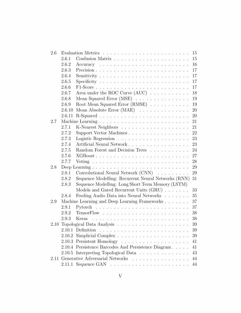
Since our hypothesis involves using machine learning and deep learningtechniques to classify depression, it was necessary for us to understand whichmachine learning frameworks were available, to aid us in implementationand experimentation. Our team consisted of undergraduate students whowere proficient in coding Python, so we decided to explore top deep learningframeworks that use mainly Python. According to the article by (Sayantini,2019), among such frameworks, Keras, TensorFlow and PyTorch are mostpreferred by data scientists and students working in the fields of machinelearning and artificial intelligence. Figure 31 compares Keras, TensorFlow,and Pytorch based on their popularity.

2.9.1 Pytorch

Pytorch is an open-source deep learning framework backed by Facebook,inspired by Torch, another deep learning framework based on Lua (Vu, 2019).Pytorch offers fast runtimes and high performance, as it runs on Pythonwithout using high level application interfaces. Furthermore, researchers candebug training models with existing Python debuggers such as PyCharm,

37

pdb, ipdb and even conventional “print()” statement according to the articleby (Vu, 2019). Pytorch can handle large data sets and it is customizable alongthe implementation of training models. Despite its advantages, Pytorch is avery young framework compared to TensorFlow. As such, it has a smallercommunity than Tensorflow.

2.9.2 TensorFlow

TensorFlow is backed by Google. As a mature framework, it offers astronger community than Pytorch. Unlike Pytorch, TensorFlow has bothhigh level and low level programmable interfaces. It also offers high perfor-mance with superior tensor visualization. One thing that TensorFlow fails toprovide is debugging. The article by (Sayantini, 2019) also mentioned thatmany programmers found Tensorflow to be difficult to debug as they trainedthe models.

2.9.3 Keras

Keras is a high-level programmable interface which simplifies the complexarchitecture of low-level deep learning frameworks. It also runs on top ofother frameworks such as TensorFlow, Microsoft CNTK and Theano accord-ing to the article by Kevin Vu (Vu, 2019). As it provides simple architecturewith which to build a model, it is used primarily for educational and rapid-prototyping purposes. As simple as it is to use, Keras lacks the capability ofhandling large data sets, and has considerably slower performance than theother two deep learning frameworks mentioned above (Sayantini, 2019).

38

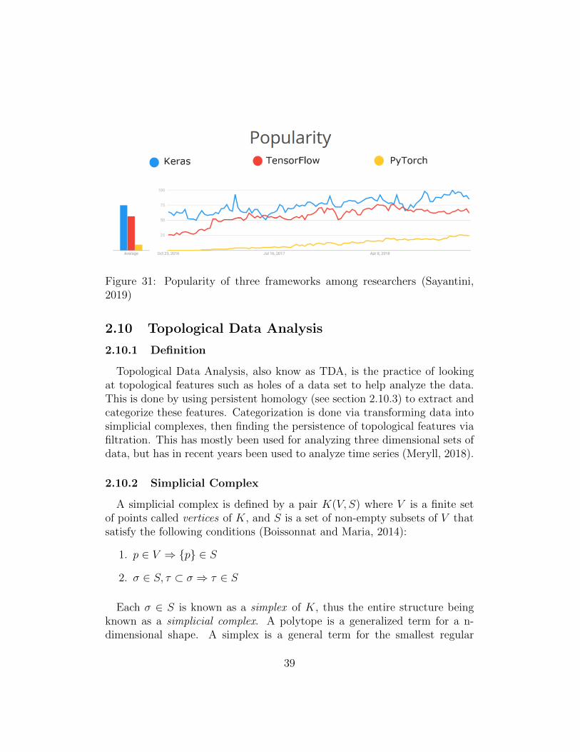
Figure 31: Popularity of three frameworks among researchers (Sayantini,2019)

2.10 Topological Data Analysis

2.10.1 Definition

Topological Data Analysis, also know as TDA, is the practice of lookingat topological features such as holes of a data set to help analyze the data.This is done by using persistent homology (see section 2.10.3) to extract andcategorize these features. Categorization is done via transforming data intosimplicial complexes, then finding the persistence of topological features viafiltration. This has mostly been used for analyzing three dimensional sets ofdata, but has in recent years been used to analyze time series (Meryll, 2018).

2.10.2 Simplicial Complex

A simplicial complex is defined by a pair K(V, S) where V is a finite setof points called vertices of K, and S is a set of non-empty subsets of V thatsatisfy the following conditions (Boissonnat and Maria, 2014):

1. p ∈ V ⇒ {p} ∈ S

2. σ ∈ S, τ ⊂ σ ⇒ τ ∈ S

Each σ ∈ S is known as a simplex of K, thus the entire structure beingknown as a simplicial complex. A polytope is a generalized term for a n-dimensional shape. A simplex is a general term for the smallest regular

39

polytope in a given dimension, such as a triangle or a regular tetrahedron. Forsimplicial complexes, we look at the connections between these simplicies. Anexample of a simplicial complex can be seen in Figure 32, in which simpliciesare created via considering the intersections of circles around each point. Inthis particular example, each circle has the same radius, however this is notrequired to form a simplicial complex.

Figure 32: Example of constructing a simplicial complex (Meryll, 2018)

Filtered Simplicial Complex A filtered simplicial complex, or filteredcomplex, is a nested sequence of simplicial complexes such that

K0 ⊂ K1 ⊂ K2 ⊂ · · · ⊂ Kn

For any Ki, i is known as the filtration level of Ki. Notably, a subset ofa simplicial complex can contain the same number of points as the originalcomplex, but different connections between points. An example of a filteredcomplex can be seen in Figure 33.

Figure 33: Example of a Filtered Complex (Bubenik, 2017)

40

2.10.3 Persistent Homology

Persistent homology observes how the topological features appear and dis-appear over a filtered complex. The persistence of a feature is defined by apair (i, j) such that i is the filtration level at which the feature appears andj is the filtration level at which the feature disappears. These are referredto as the birth time and death time of the feature respectively. An exampleof a feature that could be tracked is whether a component in the complexis connected to the rest of the components in a complex. In this case, afeature would start when a component is added, and end when the compo-nent is connected to another component. This type of feature is known as a0-dimensional hole.

2.10.4 Persistence Barcodes And Persistence Diagram

Figure 34: Example of a Persistence Barcode of a Filtered Complex. H0 is0-d holes, as explained in the above paragraph. Multiple steps of a filteredcomplex are show, and at each picture the number of lines in the barcode isequal to the number of 0-d holes in the shown complex (Ghrist, 2008)

The persistent homology of a filtered complex can be represented as eithera persistence barcode or a persistence diagram. Both consider the ”birth”and ”death” date of the topological features tracked. A persistence barcode

41

(Figure 34) represents the distance between a birth and death time as a linebetween filtration levels. This represents the persistence of each feature asa distinct interval over filtration levels, after which each interval is displayedover filtration levels.

Figure 35: Persistence Diagram of a Filtered Complex Formed from a SoundClip. This particular clip was from the DAIC-WOZ data set (see section2.3.1. Each point corresponds to the birth and death date of a feature in thesound clip

A persistence diagram represents a birth date as a x coordinate and thedeath date as a y coordinate on a graph (Figure 35). Both persistence bar-codes and diagrams of these provide useful information on the shape of thedata, however this information is much more useful to a human than a ma-chine. Disjoint intervals or points representing the persistence of features donot provide much information on how these features interact or compare to

42

one another, but as humans we can discern this information visually. Thus,we strive to combine all of these features into a single data source, so it caneasily be interpreted by a machine.

2.10.5 Interpreting Topological Data

To interpret the persistence of features as useful data, we used BettiCurves. This method transforms the persistence barcode of a filtered com-plex into a single line, which can easily be represented as a 1-dimensionalarray in data, thus easily forming a feature set for machine learning.

Figure 36: Example of constructing a Betti curve with 100 components froma persistence barcode. Unlike Figure 34, the features tracked have varyingbirth dates

A Betti curve represents the sum of lines in a persistence barcode overfiltration levels. To do this, each line in the barcode is considered as a oneif active or a zero if not. Then, the barcode is sampled over the filtrationlevels at n equally spaced points. At each point, the number of active linesin the barcode is totaled, and added to the curve. This n defines the numberof components in the Betti curve. This leads to a curve which provides agood linear representation for the original barcode, which has the distinctadvantage of being easier to construct compared to other methods. Thesecurves were first defined in a 2017 paper which explored classifying timeseries using TDA (Umeda, 2017). In 2019, another group used Betti curvesfor classification of arrhythmias from heartbeats, and found favorable resultsas mentioned in Section 1.2.5. Because we will be using TDA to classifysound, which is a form of time series, we decided to use this method.

43

2.11 Generative Adversarial Networks

Figure 37: Diagram of GAN Process (Goodfellow et al., 2014)

Generative Adversarial Networks (GANs) are generative machine learningsystems. GANs work by training two distinct networks, generator G, whichlearns to generate samples from a given data set, and discriminator D, whichtries to discern fake samples generated by G from real samples. Fundamen-tally, the two are playing a minimax game, where G is trying to maximizethe number of generated samples that D thinks is real, while D is trying tominimize the number of generated samples that are chosen. Figure 37 showsthe general flow of how GANs work. With enough iterations, G will eventu-ally converge and produce samples that D cannot distinguish from the realsamples.

2.11.1 Sequence GAN

44

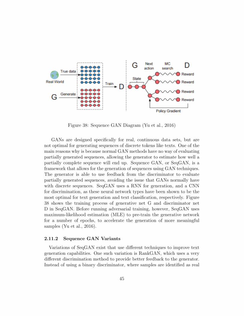
Figure 38: Sequence GAN Diagram (Yu et al., 2016)

GANs are designed specifically for real, continuous data sets, but arenot optimal for generating sequences of discrete tokens like texts. One of themain reasons why is because normal GAN methods have no way of evaluatingpartially generated sequences, allowing the generator to estimate how well apartially complete sequence will end up. Sequence GAN, or SeqGAN, is aframework that allows for the generation of sequences using GAN techniques.The generator is able to use feedback from the discriminator to evaluatepartially generated sequences, avoiding the issue that GANs normally havewith discrete sequences. SeqGAN uses a RNN for generation, and a CNNfor discrimination, as these neural network types have been shown to be themost optimal for text generation and text classification, respectively. Figure38 shows the training process of generative net G and discriminator netD in SeqGAN. Before running adversarial training, however, SeqGAN usesmaximum-likelihood estimation (MLE) to pre-train the generative networkfor a number of epochs, to accelerate the generation of more meaningfulsamples (Yu et al., 2016).

2.11.2 Sequence GAN Variants

Variations of SeqGAN exist that use different techniques to improve textgeneration capabilities. One such variation is RankGAN, which uses a verydifferent discrimination method to provide better feedback to the generator.Instead of using a binary discriminator, where samples are identified as real

45

or fake, RankGAN gives the discriminator a list of samples, which the dis-criminator then ranks. This feedback contains considerably more informationto learn from, allowing the generator to learn more from fewer epochs (Linet al., 2017).

Another variation is LeakGAN, designed specifically to work with longertexts. In normal SeqGAN, the discriminator only provides binary feedbackafter the entire sample has been generated. LeakGAN allows the discrimi-nator to leak the kinds of features it looks for to the generator, which thegenerator uses at all steps of generation to produce better, longer samples.Figure 39 shows the flow of LeakGAN, showing how the discriminator showsits internal state to the generator (Guo et al., 2017).

Figure 39: LeakGAN Flow Diagram (Guo et al., 2017)

46

RelGAN is a recently-developed sequence GAN method that builds uponthe work of previous previous sequence GAN studies. RelGAN uses rela-tional memory in the generator, instead of the traditional RNN or LSTM, toallow for a more expressive text generator. Additionally, RelGAN uses lessdemanding reinforcement learning heuristics for training, and multiple rep-resentations for each generated sequence in the discriminator. All of this hasshown that RelGAN outperforms other sequence GAN methods consistently(Nie et al., 2019).

2.11.3 Sequence GAN Evaluation Metrics

Different metrics are used to evaluate the performance of sequence GANs.One metric specifically developed in the SeqGAN paper is NLL-oracle loss(Negative Log Likeliness). NLL-oracle loss randomly initializes an LSTM tobe treated as the oracle, which is compared with the generator to producea value that the GAN minimizes as it runs through multiple epochs. Figure40 shows the NLL metric, where G(theta) is the generator, and G(oracle)indicates the oracle model. For NLL, lower values are considered better, asNLL represents the entropy to be minimized in the model (Yu et al., 2016).

NLLoracle = −EY1:T∼Gθ[

T∑t=1

log(Goracle(yt|Y1:t−1))]

Figure 40: NLL-Loss (Yu et al., 2016)

BLEU (Bilingual Evaluation Understudy) score is another metric that canbe used, specifically used for evaluating texts generated by SeqGAN variants.BLEU score was originally developed as a metric for evaluating machinetranslation, but has become the standard metric for evaluating all machine-generated text. BLEU is a ”translation closeness” metric, which comparesa generated sample to a corpus of group of good samples. For machinelearning purposes, this corpus is usually the training data. BLEU scoresrange from 1.0, which means that the generated sample exactly resemblesone of the samples in the corpus, to 0.0, which means that the generatedsample does not resemble one of the original samples at all. Since a score of1.0 indicates that the neural network has just replicated one of the given real

47

samples, BLEU scores in the 0.6-0.9 range are considered better (Papineniet al., 2002).

3 Feature Extraction

3.1 Text Feature Extraction for Machine Learning

To extract features, we started from a script that was made for the paper”Screening for depression with retrospectively harvested private versus publictext”. This script made use of ”word category frequencies, part of speech tagfrequencies, sentiment, and volume” (Monica Tlachac, 2020) features. Thisscript generated features using the tools: Empath and Textblob. The scriptmakes use of TextBlob’s Part of Speech tags, as well as custom sentimentfeatures from the TextBlob output. We modified the provided script to makeit to work for the DAIC-WOZ data.

The script reads in a file with three columns: ID, which contains theparticipant ID, and question number, Content, which contains what the par-ticipant replied, and PHQ-8 Score, which is simply the participant’s PHQ-8score. The script produces a .csv file with a numbered first column, a sec-ond column with ID(participant ID and question number), score(the PHQ-8score), followed by 245 columns of features that were extracted.

3.2 Audio Feature Extraction for Machine Learning

3.2.1 Pratt

To extract the audio features from DAIC-WOZ, we decided to use thePratt script from the 2019 Major Qualifying Project to extract pause timefeatures. We realized that some of the clips from our processed DAIC-WOZdata set included numerous empty clips, So we modified the script to preventif from if there was no audio in the clip.

On each run through a directory, the script uses for parameters that de-termine how the features are extracted. The first is silence threshold, whichrelates to the dB value needed for the program to classify the clip as a pausein the conversation. The second parameter is minimum dip between peaks.

48

The third parameter is minimum pause duration, which refers to how longthere has to be silence at the silence threshold for it to be considered a pause.

The program outputs the file ID, the number of syllables, the number ofpauses, the duration of the audio file (in seconds), the vocalization time (inseconds), the pause time (in seconds), the speech rate (number of syllablesdivided by the duration of the audio clip), the articulation rate (the numberof syllables divided by the vocalization time), and the speaking time, dividedby the number of syllables. The program outputs it to the Pratt interface,which is then copied into a .csv file.

For the first trial, we run the Pratt script on 2-5 second audio clips fromDAIC-WOZ. We set the parameters as follows: silence threshold of -25dB,minimum dip between peaks of 2dB and minimum pause duration of 0.3 secs.

Due to the high volume of data that it would need Praat feature extraction,we modified it to work on the cluster.

3.2.2 openSMILE

openSMILE is an audio extraction software used for signal-based features,unlike Pratt which is used for pause-time features. The feature extraction onopenSMILE is done using the 2010 Embrosa configuration and is being usedto generate 1600 features per audio clip.

3.3 Topological Data Analysis

To use data in topological data analysis, it much first be transformed into afiltered simplicial complex (see section 2.10.2). To do this, we use the Gudhipython library2 using simplicial trees. Simplicial trees are a data structurethat efficiently represents simplicial complexes in data using a tree structure,and is what Gudhi uses to represent simplicial complexes (Boissonnat andMaria, 2014). Gudhi is a python library dedicated to performing topologicaldata analysis, and was the most simple to use due to being used in previousefforts in implementing Betti curves.

2https://gudhi.inria.fr/python/latest/

49

3.3.1 Constructing Filtered Complex From Sound Waves

To construct a filtered complex from sound waves, we consider each segmentof the wave as a path between two vertices, then link these paths togetherto create the full wave. Then we assign filtration levels to each segment suchthat where 0-d holes appear and disappear are at local maxima and minimaof the wave. This is done by considering the magnitude of the sound wave ata particular point as its filtration level. Thus, the holes appear and disappearat minima and maxima. This can be seen by observing the following seriesof diagrams:

First, we can see the wave as a hole, before filtration is applied.

Filtration Level

Magnitude

Figure 41: A Simplicial complex from a simplified sound wave

Next, the smallest values are added.

50

Filtration Level

Magnitude

X0

Figure 42: First Filtration Level of Wave Filtered Complex, X0. Each seg-ment with a filtration level less than X0 is added

Then, the first segment on the left is created, making the first hole.

Filtration Level

Magnitude

X0

X1

Figure 43: Second Filtration Level of Wave Filtered Complex, X1. Eachsegment with a filtration level less than X1 is added

51

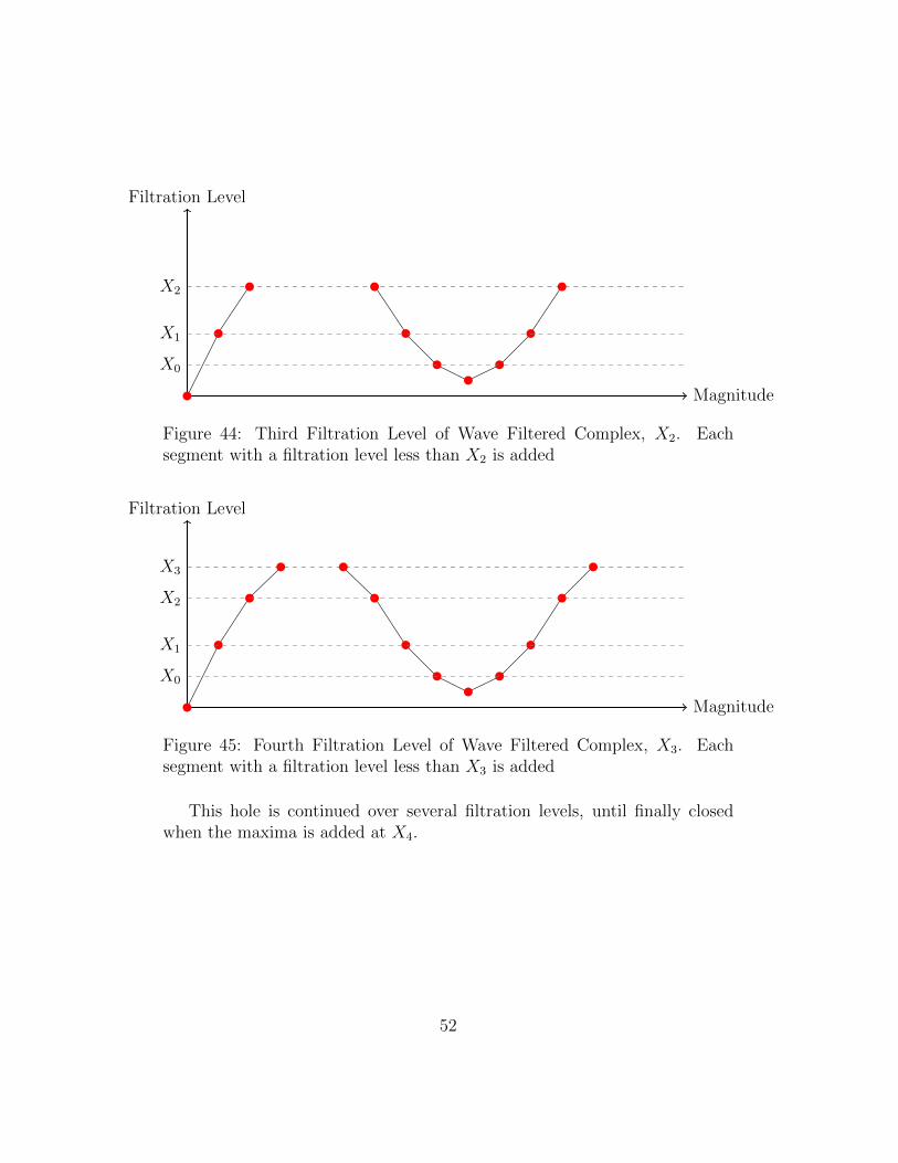
Filtration Level

Magnitude

X2

X0

X1

Figure 44: Third Filtration Level of Wave Filtered Complex, X2. Eachsegment with a filtration level less than X2 is added

Filtration Level

Magnitude

X3

X2

X0

X1

Figure 45: Fourth Filtration Level of Wave Filtered Complex, X3. Eachsegment with a filtration level less than X3 is added

This hole is continued over several filtration levels, until finally closedwhen the maxima is added at X4.

52

Filtration Level

Magnitude

X4X3

X2

X0

X1

Figure 46: Fifth Filtration Level of Wave Filtered Complex, X4. Each seg-ment with a filtration level less than X4 is added

This is how our filtered complexes were constructed, insuring that per-sistent homology captures the critical points of the sound wave. We alsoconsider filtration from maximum value to minimum value, and differentiatethe two by calling minimum to maximum ”upper level” and maximum tominimum ”sub level”. We do both of these as the persistence captured canvary slightly based on when features appear and disappear. Next, we convertthese into barcodes, followed by Betti curves, whose construction is coveredin Section 2.10.5. This is the final state of our topological features extractedfrom sound waves, after which they can be inserted into a machine learningmodel.

Figure 47: TDA Feature Extraction Pipeline

53

Figure 48: All combinations of method, data set, feature type, goal, andprediction type in this paper

54

3.4 Generative Adversarial Networks

The SeqGAN variants used only raw text data from EMU and Moodable,without extracting specific features, as the goal was to expand that data setand extract features from the texts generated by it.

4 Methods

4.1 Machine Learning

In this project, we implemented regression and classification methods forsix models: Support Vector Machine, Random Forest, XGBoost, AdaptiveBoosting, k-Nearest Neighbours, and Multilayer Perceptron. We conductedvarious tests for each method and model variation to find best performingones. Through out the project, we were able to build an Machine Learningefficient pipeline to conduct experiments on three different data sets: EMU,Moodable, and DAIC-WOZ. Although most of our experiments were tar-geted at predicting PHQ-8 labels, we had experiments that predicted GAD-7 Labels for EMU data set. Overall, our goals within this sub project werecomparing Machine Learning method performances across different datasets’Experimentation.

4.1.1 Machine Learning Pipeline

For our Machine Learning methods, we first sliced the audio data intosub-clips. Further, we supplemented the audio clips with Sub-Clip Boost-ing (which was shown to improve scores (Toto et al., 2019)) implementingoverlaps between the sub clips. After successfully slicing our audio data,we generated features using openSMILE and Praat tools. Resulting featurefiles were cleaned and labelled with corresponding labels: PHQ-8 or GAD-7. After generating fully labelled clean feature files, we performed featureselection to get the optimal number of features for our experiments. Next,we split feature files into their respective folds. Splitting is done by usinga json file that contains participant IDs used to determine whether partic-ipants are allocated in either train or test sets. These splits were kept thesame throughout all experiments. After participants within feature files weresplit into train/test sets, we used a grid search to tune optimal parameters forthe models. Some models didn’t compute grid search within computational

55

time thus random set of parameters were tested on and the best performingones were selected. Next, using parameters generated from grid search, wefit classifier and regressor models. After models are fitted with training dataset, we use these fitted models to predict our testing data set to get ourresults. The generated results contain binary classifications and regressionpredictions. In addition, they contain prediction probabilities.

Figure 49: Machine Learning Pipeline

Figure 49 illustrates our pipeline process. Bold and underlined stepsrepresent main processes, while the boxes below main processes representsub processes.

4.1.2 Machine Learning Method Configurations

Data Processing: DAIC-WOZ Audio For DAIC-WOZ audio, we firstsplit participant audio data into question segments. We further broke thequestion splits into Sub-Clips based on clip duration. Intervals of 3, 4, 5, 6,7, 8, 9, and, 10 seconds were used. Once data were split into sub clips, weimplemented SCB (Toto et al., 2019) to enhance our experiment scope. ForSCB, overlapping of 0%, 25%, 50%, and 75% were used to boost clips.

Data Processing: DAIC-WOZ Transcript+ Audio For DAIC-WOZaudio, we first split participant audio data into question segments. We then

56

organized the transcripts into question segments and made sure the samenaming conventions as the audio data were used.

Data Processing: EMU For EMU data, we split participant audio datainto Sub-Clip splits. Sub-Clips with 2,3,4,5,6,7 segment splits were used.Once data were split into sub clips, we implemented SCB to enhance ourexperiment scope. For SCB, we used the standard overlapping intervals asthe DAIC-WOZ processing technique.

Data Processing: Moodable We used the exact same technique used toprocess EMU data for processing Moodable data.

Feature Selection: openSMILE Feature selection was implemented foropenSMILE features due to large number of features. Firstly, we used ExtraTrees to determine the features’ importance. Next, we kept features that hadfeature importance higher than the mean feature importance. We used sci-kit libary’s ((Buitinck et al., 2013) ExtraTreesClassifier() tool. We invokedthe resultsing model’s attribute feature importance to get feature importancevalues. Resulting dataset had a reduced set of 176 features.

Participant Splits Participant splits were mainly done using a script thatgenerates 5 folds and randomly allocating participants within those folds.These folds were stored in a json file and maintained throughout experi-ments. For example, a fold split for EMU GAD-7 dataset would be usedacross all EMU GAD-7 experiments. This approach was done for Mood-able, DAIC-WOZ and EMU PHQ-8 experiments. However, we added twoextra folds for DAIC-WOZ dataset. This was done to enable result com-parisons with other researches using DAIC-WOZ dataset and amongst ourDeep Learning and LSTM experiment results. The particiapnts were splitinto train and test splits for this part instead of maintaining cross validationapproach mentioned earlier. For comparing with other researches we usedthe DAIC-WOZ official splits: train split and dev splits. Dev splits wereinterpreted as our testing set and train split was used as training set. Tocompare with our Deep Learning and LSTM models, we used a train andtesting split determined randomly. Data set was split into 70 to 30 ratio infavor of training set. In addition the Depressed and Non-Depressed partic-ipants had same ratio in both splits. We used a standard cutoff of 10 as a

57

binary cutoff.

Training We fitted the data on the Machine Learning methods mentionedearlier. We used grid search to determine optimal parameters for our modelswhen possible. However, since this was computationaly expensive we opted toselect optimal parameters out of a random set of parameters for our models.

For Random Forest, we found the best parameter selections to be: 400estimators, maximum depth of 7 for the trees, minimum samples split of 5,minimum sample leaf of 1. These parameters were used in both regressorsand classifier models.

For K-Nearest Neighbours, we found best parameter selections for numberof neighbours and leaf size to be 9 and 1 respectively.

For XGBoost, we selected inputs for the parameters learning rate, gamma,maximum depth of tree, minimum child weight, subsample, colsample bytree; Values for these parameters were 0.01, 5, 4, 1, 0.7, 0.6 respectively.

For Support Vector Machines, we were only able to use linear kernels dueto computational issues. Thus, we weren’t attain optimal parameters for themodel.

For Adaptive Boosting, we used a Random Forest with the previouslymentioned parameters as a base estimator. In addition, we used 400 trees asestimators.

For Multilayer Perceptron model, we used an L2 penalty of 1, maximumnumber of iterations of 50, solver was stochastic gradient descent, a learningrate that is adaptive (keeps the learning rate constant to initial learning rateas long as training loss keeps decreasing), initial learning rate.

Predictions Our Machine Learning experiment framework outputs testpredictions in a csv file format. The files contain binary predictions, bi-nary prediction probablities, and regression predictions for each participantSub-Clip features. These are later aggregated to have predictions for partic-ipants. Note, in the case of DAIC-WOZ dataset experiments aggregations

58

were done based on questions as well. Once aggregated we evaluate pre-dictions by computing TN, TP, FP, FN, accuracy, sensitivity, precision, F1score, specificity, MAE, RMSE, R2, MSE. We also determined a cutoff forour regression predictions in order to compute F1 score and compare with aclassification approach. Grouping of predictions were done based on differentaggregating methods: median, mean, max and voting. We also used a weightthat was altered during experiments. The participant was elected to be de-pressed if the binary prediction probability of one (Depressed) multiplied bythe determined weight was higher than the binary prediction probability ofzero (Non-Depressed). In addition, we used F1 score as the standard metricto compare different experiments.

4.2 Deep Learning

In order to use Deep Learning for mental health sensing, we first neededto implement data-preprocessing on our available data set. We primarilyintended to use DAIC-WOZ data set so that we could produce results com-parable to other techniques like machine learning and DepAudioNet. Forthe purpose of building and debugging our first deep learning pipeline, westarted with combined EMU and Moodable data set since testing on themis less resource-expensive than DAIC-WOZ data set. At the same time, wealso built data-preprocessing on DAIC-WOZ data set. Once we made sureour deep learning pipeline is free of syntax and compilation error, we beganfinding an efficient model by gradually testing out various hyperparameterssuch as number of layers, learning rate and kernel sizes. Then, we analyzedeach of our deep learning models by confusion matrix, convergence of trainloss and test loss curves, F1 score and accuracy.

4.2.1 CNN Experimental Setup

Our goal here was to see if we could build our own convolutional neu-ral network that was able to train on one of the available data sets. Forthe EMU/Moodable data set, data preprocessing was already done prior toworking with those data sets, so we were able to begin by start by definingconfigurations and laying out python source code to fit our new model. Thesetup we built here is similar the one in Figure 22, except that we tweakedthe parameters to suit our data. We started with minimal amount of config-urations to see the changes and compare them as we tune them.

59

• Hyper parameters: Batch-size was set to 1 and would gradually increaseup to 16. Number of epochs was kept at 60 since more would take alonger time to finish. The optimizer used here is Adam with learningrate set up to 1.5e-7.

• CNN structure: Input was a 2D array of spectrogram data with re-spective labels of PHQ-8 scores. These PHQ-8 scores were taken in asnon-depressed with scores below 10 and depressed with scores between10 and 24. The output in this case was binary classification with de-pressed as 1 and non-depressed as 0. Therefore the loss function usedhere was cross entropy loss for binary classification. The model hadtwo two-dimensional convolutional layers and two max pooling layers.The first convolutional layer had (3x3) kernel, and step size or strideof 1. The first max pooling layer used (4x3) kernel, and with a strideof 3. The second convolutional layer had (1x3) kernel, and stride of 1.The second max pooling layer uses (1x3) kernel, and stride of 3. Thetest data set of 30 percent was from the original data sets.

• Feed-Forward network: the output we have from CNN was flattened asa one-dimensional array and then fed into this multilayered perceptron.Here we had two more hidden layers: one with flattened array size andanother with 512 nodes. The drop out layer with 0.15 was added toreduce over-fitting. The output layer matched two number of classeswhich were depressed and non-depressed.

4.2.2 LSTM Experimental Setup

The goal of our sequence-based model was to exploit the ability of anLSTM network to remember information and use context. There are a fewdifferent ways in which our data can be treated sequentially. We brieflyexplored inputting spectrogram images of DAIC-WOZ data, before focusingon features generated with openSMILE. Our first batch of experiments wasusing a set of 25 openSMILE (os25) features, selected as the most impactful.After getting better results using a more verbose set of 176 features (os176)we ran the rest of the experiments on this set. The final model was builtusing PyTorch.

• Structure: The data was first fed through an LSTM layer, the outputof which was then passed through a linear layer and finally through

60

a sigmoid output layer. The loss function was binary cross-entropy,and we experimented between AdaDelta, RMSProp, and Adam foroptimizers.

• Data: The openSMILE features were stored in a .csv file. Each rowrepresented the features for one sound clip. We used 3 second clipswith 0.75 overlap between clips. The data was grouped by questionand given a label, meaning that each time step was a sound clip for thequestion. Predicting label for an entire question gave the best results.The model predicted binary label, giving a cutoff of 11 and above asdepressed, below as non-depressed. During experiments, the originaldata (in order by participant and question) was split at 70% for thetraining set, and the remaining 30% as validation. To compare resultswith other models in this project, the best models were re-trained withthe same split as the rest of the deep learning and machine learningsolutions.

• Hyperparameters and settings: Learning rate was {1e-5, 1e-6, 5e-7, 1e-7, 1e-8, 1e-9}, hidden nodes were {50, 100, 150, 250}, and number oflayers was {1, 2, 4, 6}. Dropout rate was {0, 0.1, 0.2, 0.5, 0.8, 0.9}.

4.2.3 Deep Learning Pipelines

CNN The first thing that needed to be done before other steps was dataprocessing. This step included collecting audio files, limiting question num-bers per participant, and extracting PHQ scores and gender labels. Afterthat, the whole data set was divided into training set and testing set. Whilesplitting into two separate data sets, data balancing was also performed onthe training set to avoid failing to recognize the minority class. The trainingprocess began when we had balanced training set and testing set. Duringthe training process, we started off with CNN layer configurations as statedabove in Experimental Setup. However, hyper parameters such as kernelsizes and number of dense layers were subject to changed as we were tryingto find a decent model through multiple experiments. Gender label werealso added into fully connected network after receiving feature map throughconvolutional process. Once the training process was done, the model waspredicted with testing set and the confusion matrix was collected.

61

Figure 50: Convolutional Neural Network pipeline

LSTM As with the CNN, data preprocessing was done first as described inSection 4.3. The LSTM model mostly used the 3 second clip length with 75%overlap. openSMILE was used to extract features for each clip. At this point,the fill data set was a .csv file with each row containing the feature set forone clip. Here, the data was split into a train and a test set. Then, the clipswere grouped by individual question response and paired with the depressionlabel of the participant answering (for the sequence model we used a PHQ-8

62

score of equal to or less than 10 to mean non-depressed, and higher than 10as depressed). We then trained our model on this data, validating at the endof each epoch with the test set. After every epoch we collected metrics aboutthe performance. These included the hyperparameters and settings used, theloss and accuracy of the train and test sets, and the confusion matrix valuesfor the test set which was used to calculate precision, recall and F1 score.Both in real-time and after training has completed, these metrics could bepassed to a custom performance analytics and visualization tool in a Jupyternotebook to examine how the model was doing.

Figure 51: Sequence Model (LSTM) pipeline

4.2.4 Experimental Planning

63

Figure 52: Workflow between Image Caching and without Caching

Reducing Training Time The difference in size of EMU+Moodable datasets and DAIC-WOZ data set is vast. While the combined EMU and Mood-able only has 290 audio files, DAIC-WOZ contains 10570 audio files. Thecurrent setup we have would work on EMU and Moodable for a consider-able amount of time, it could take over a week to process and train rawaudio files from DAIC-WOZ data sets. One way was to implement a cachingsystem that would boost up the speed of the experiments using the sameconfigurations for generating the spectrograms. For example, if we decidedthe spectrogram to have one dimensional tensor of 256 by 64, 1024 slicesand 1000 overlaps, the other experiments that used the same spectrogramconfigurations would not need to generate extra cache. This would allow usto train the DAIC-WOZ data sets over a day with more epochs.

64

One promising way to reduce training time for both CNN and LSTMmodels is node or weight pruning. The concept here is that by orderingneurons or weights by how much they contribute, the lowest-ranking can beremoved (Le Cun et al., 1990). The paper by (Molchanov et al., 2016) detailsan iterative process for pruning CNNs by ordering nodes, removing the last,testing the affects, then continuing on to the next if needed. There are alsomethods of removing entire filters from the CNN instead of single weightsor nodes (Li et al., 2016). Similar concepts can be applied to LSTM-basedmodels, to see similar results.

LSTM Workflow Running experiments, changing parameters, generatingand comparing results, and editing code can all make developing deep learn-ing models very time-consuming. We have created some tools to automatethis process. For the LSTM model, hyperparameters and other options likethe optimizer, learning rate, number of hidden nodes and layers, and dropoutrate are passed from the command line. Metrics such as loss and true andfalse negatives and positives, are collected after each epoch and saved to afile. When running a test, a bash script is run to submit the job to the jobmanagement system on our research cluster, Slurm. In this way, when wehave an experiment to run, we can write a script to submit all the relatedjobs with their individual hyperparameters in parallel. Once the experimenthas finished, we can pass the directory where we saved the metrics for eachrun to a metrics utility. This utility graphs the loss over time, as well asaccuracy, precision, recall, and F1. It also displays the confusion matrix forthe last epoch. This same file doubles as a log of experiments, keeping trackof their hyperparameters, settings, Slurm job ID’s, and additional notes.

In addition to saving metrics, the states of the model and optimizer aftereach epoch (weights and parameters) were saved to disk as a .pt file withPyTorch’s built-in method. If a model showed that loss, accuracy, or F1 hasnot yet stabilized, we could submit a new job that would load the modelback in and continue training from where we left off. Some later experimentswere run up to 800 epochs in 200 epoch chunks until metrics stabilized, orit became apparent that the model was overfitting. This was only necessarydue to the computation time limit on the research cluster.

CNN Since we could not know which CNN model was going to performbest for detecting depression, we needed additional planning and multiple ex-

65

periments to compare the results. Here, we could proceed in two approaches.One was to simplify the CNN structure to 1 convolution and 1 max poollayer and figure out the number of layers and kernel sizes that might workfor our data sets. The advantage of this plan was that once we figured outthe right setup, we could continue training and predicting other data setswhich are similar to DAIC-WOZ or EMU and Moodable data sets. Thedownside was that we would have to continue testing each setup until wefind out a proper model. Another one was to test with other features such asopenSMILE along with convoluted features. With this approach, we couldtune the feed forward network properly and observe if openSMILE improvedmodel learning or not.

Convolution & openSMILE Experimenting with CNN alone on DAIC-WOZ data sets was quite challenging and unpredictable. Since convolutionlayers filtered out the features from each spectrogram by kernels and maxpooling, the feature set we could get from convolution may not be as distin-guished as other feature sets such as openSMILE. Thus, we could also speedup our experiments by combining CNN with other feature set. For example,we could determine if a model improved predicting by combining feature setgenerated from Convolution layers and respective OpenSmile Features andthen fed them together into the same Feed Forward Network.

66

Figure 53: Combining Convolution and openSMILE

openSMILE From the above premise, we could also derive experimentsto test openSMILE features and Feed Forward Network only. By doing so,we could find significant parameters which would substantially impact ourmodels inside Feed Forward Network. Since these experiments would notconsist of Convolution layers, another advantage was that they would requireless computational resources and could complete in a shorter amount of timescompared to CNN experiments.

Parameter tuning Parameter tuning would be done in all experimentsbut there were specific parameters we considered might have big impact inimproving our learning models. Besides from convolution and feed forwardlayers, parameters such as learning rates and decays played a huge part inimproving our models. Learning rate referred to the amount at which theweights were updated every epoch. Learning rate that was too large couldlead the gradient descent to step over the global minimum and too smallcould make it stick at the local minimum (Brownlee, 2019). Decay rate asa multiplicative factor would be applied to learning rate. The reason usingdecay rate was that we wanted to allow the model to converge faster at theearlier epochs and slower towards the end so that it would avoid local min-

67

ima and had a better chance of finding a global minimum. Mathematically,learning rate at every epoch is as follow with ”t” being the current epoch.

LearningRatet = LearningRatet−1 ∗DecayRate (1)

4.3 Tests Run on Audio Data

We divided the DAIC-WOZ audio files by question response, with a foldercontaining the response for each question by each participant. We thenproceeded to divide each file by three seconds. When the split was done, anyresponse less than three seconds was disregarded. Audio files that were morethan three seconds were split into full three second clips and the reminder wasalso disregarded. This was then repeated for four,five,six and seven seconds.All splitting and processing was done by scripts on the cluster.

4.4 Tests Run on Transcript

DAIC-WOZ came in two parts: audio data and the transcript data. Weprocessed the transcript data to organize replies by participant and questions.We extracted features from this using Textblob and Empath.

Figure 54: Frequency Graph for Transcript Data (Ali, 2018)

68

Figure 55: Histogram of Transcript Data (Ali, 2018)

As you can see in the above figures, the number of words in a questionresponse varied. The number of words ranged from one, all the way up to120 words. We set up a script to feed the pre-processed transcript data(a .csvfile) and number for the minimum number of words allowed. For example,when we fed it the file and the number four, it made sure all responsesthat were under four words was filtered out. This is good because responseswith few words would give less features and yield lower lower results. Weexperimented with 4,7,and 10 word minimums.

4.4.1 Tests Run on Audio and Transcript

The next step was to combine both audio and transcripts to attempt toget the best results. It was unrealistic to combine the sliced audio and getthe transcript for that without doing it manually for tens of thousands ofclips. So, the reasonable process was to do it question by question. So, weran the pipeline through each question response audio clip. We then selectedthe text features for the transcript data and used a script with the mergecommand to merge the two. The result was that each row would containboth the audio features and transcript features for a question reply.

69

4.5 Topological Data Analysis

To test the viability of Betti curves (see section 2.10.5), we used ma-chine learning methods similar to that of Section 4.1. Our data sets usedall stemmed from five second DAIC-WOZ clips with no overlap, with differ-ent selections from these clips being used in training. To prepare, upper leveland sub level Betti curves for each participant were extracted into separatefolders, then several data sets were constructed by pulling specific curvesfrom each participant. These included random 5 curves, the first curve foreach question, and the first 5 curves. Another data set was also made whichcombined the openSMILE features of the first 5 clips from each participantwith the first 5 curves from each participant. This is done using a truncatedversion of openSMILE with only 176 features. For each data set, both aupper level and sub level set is formed separately. In total, this leaves uswith 8 unique data sets. After each data set is formed, they are fed throughdimensionality reduction using PCA, kPCA, and Chi2 (see section 2.4). Chi2

chooses up to the total number of features, leaving at least one data set withall features. kPCA and PCA both choose up to 15 features. After this iscomplete, each data set is fed through a series of machine learning mod-els: Naive Bayes, Linear Regression, k Nearest Neighbor with 3 neighbors(kNN3), k Nearest Neighbor with 5 neighbors, Support Vector Classification,XGBoost with 2 levels, XGBoost with 3 levels, XGBoost with 4 levels, andADABoost. In total, we end up with 216 separate combinations of data set,dimensionality reduction, and machine learning model. The overview of theTDA machine learning pipeline can be seen in Figure 56.

70

Figure 56: Pipeline for Machine Learning Using Betti Curves

4.6 Generative Adversarial Networks

We used a number of methods for generating text based on our existingdata set. We first focused on using the Moodable data set to generate newtexts using Texygen, an open source framework designed for easily runningand comparing text generation methods (Zhu et al., 2018). We created apipeline for running sequence GAN tests. Two sets of experiments wererun: one on the ACE cluster, and one on the Turing cluster, as it had moreresources available for experiments.

71

4.6.1 ACE Experiments

Figure 57: Moodable: Ten Most Frequent Words

Before the text generation methods could be run, the text messages had tobe pre-processed appropriately. Text message data was provided in a CSVfile, which indicated the user ID the text was from, and the text itself. ThisCSV was loaded using a python package called Pandas, which allowed foreasier handling and visualization of data. Some statistics were gathered onthe data set, before breaking it into subsections based on user ID. Figure 57shows the top ten words that occur most frequently in the Moodable dataset, while Figure 58 shows the participants with the ten highest text countsin the Moodable data set.

72

Figure 58: Moodable: Ten Participants with the Most Texts

Texygen requires input files that have a single text on each line, withall of the relevant data for each run in a single file. To simplify the datathat the text generation techniques would have to learn from, the naturallanguage toolkit (NLTK) was used to find the frequencies of each word withindata subsets, and replace words that occurred less frequently than a giventhreshold with < UNK >. For the tests we ran this time, the frequencythreshold was 5.

The first experiment was run using SeqGAN, using every text from Mood-able as training data. This experiment ran out of time after twelve hours,the maximum amount of time allowed by the ACE cluster we were workingon. The data set was then simplified, using only ten-thousand texts from asingle participant, instead of using every text, but this also ran out of time.The number of epochs was then reduced from Texygen’s default number of80 pre-training epochs and 100 adversarial training epochs to only 20 pre-training epochs and 30 adversarial training epochs. The data set was further

73

simplified, only using 1074 texts from a single participant. With these pa-rameters, the experiment successfully finished within the time limit. Furtherexperiments were run using these values, for MLE training on its own (asa control group), RankGAN (as an improvement over SeqGAN), and Leak-GAN (as it performed better with longer texts). As a result of the CPUspecific requirements, GPU acceleration was not possible on the cluster atthis point.

After running these experiments, we used matplotlib to derive and plotthe NLL-Loss and BLEU scores. Other statistics were automatically gener-ated by Texygen itself, such as NLL-loss, but these were somewhat problem-atic to use, as the output CSVs generated by each text generation methodwere formatted inconsistently.

4.6.2 Turing Experiments

After ACE proved not to be optimal for running Tensorflow and RelGAN,we gained access to the Turing cluster, which allowed for far more epochs tobe run using GPU acceleration. Some further improvements were made onthe experimental process, after the rests run on ACE.

Figure 59: Text Generation Pipeline

Process Improvements The overall process was improved by modifyingthe existing frameworks. Texygen was forked and modified to accept a rangeof new command line arguments to facilitate much faster iteration of ex-periments. Arguments were added to control output file path, pre-training

74

epochs, adversarial training epochs, and CSV output path.3 Furthermore, wedeveloped a script that would automatically generate batch files for submit-ting new jobs to the Turing cluster. The pipeline created for text processingduring this stage can be seen in Figure 59.

RelGAN Additionally, RelGAN, which was not included in Texygen, wasset up to run with our data set. RelGAN does not accept most data sets bydefault, so it was also expanded to accept multiple data sets.4 Due to thedifferent requirements needed to run RelGAN, a separate batch file generatorwas created for RelGAN jobs.

5 Results

5.1 Machine Learning

5.1.1 GAD-7 Experiments on EMU

Although most experiments we did throughout this project used PHQ labels,this sub-project used GAD-7 labels to make predictions. GAD-7 have shownto be reliable predictors for anxiety, which is generally easier to predict thandepression and have more consistent symptoms (?). Generally, in our GAD-7experiments we found that tree based models and cutoff performed better.In addition, there were better results when using up-sampling compared todown-sampling. Tree based models have been shown to perform better inprevious studies as well (Yang et al., 2016). We attribute the experimentresults being skewed towards binary cutoff of 5 due to the EMU dataset’sdispersion; most participants have a GAD-7 score of less than 10. The bestperforming test runs for our GAD-7 Experiments can be seen in Figure 60.As mentioned earlier, the top 5 test runs used either XGB or ADA methods.In addition, all top test runs used a binary cutoff of 5. Models also performedbest when using our up-sampling technique; it is also evident that SCB worksbest for these experiments.

3This modified code can be found at https://github.com/Nicolas-Pingal/Texygen4This modified code can be seen at https://github.com/Nicolas-Pingal/RelGAN

75

Figure 60: Classification: GAD-7 Experiments Top F1 Scores

As seen in Figure 61, even though the F1 scores were significantly lower,most assertions about tree based methods performing better still hold true.However, in this section of test runs, down-sampling performed better. Down-sampling works better for binary cutoff of 10 as a result of the dataset be-coming more skewed towards depressed participants when using this cutoffvalue. Furthermore, SCB still seemed to improve model’s performance.

Figure 61: Classification: Best Test runs for Cutoff=10

We converted the regression predictions into binary predictions, to com-pare them with a direct binary prediction. The results were slightly lower,so it is hard to deduce any meaningful conclusions.

Figure 62: Regression: GAD-7 Experiments Top F1 Scores

76

Figure 63: F1 Score distribution across Models

Figure 64: F1 Score distributions among Resampling Techniques

77

Figure 65: F1 Score distributions among Binary Cutoffs

Original dataset experiments We were able to do an experiment usingthe original data without doing any splits or overlaps. The results were rela-tively poor compared to SCB and split audio experiment results. The highestF1 score was 0.528 with RF model and a cutoff of 10 using up sampling.

78

Figure 66: Predictions for un-split and no-overlap

5.1.2 PHQ-8 Experiments with EMU

Our experiments on the EMU dataset using PHQ-8 performed slightlyworse than our experiments using GAD-7. However, compared to previousMQP’s experiments using audio features from EMU, we found significantlyhigher results as depicted in figure 67 and figure 68. Figure 67 shows box-plots of all model experiments. Highest F1 score across all model tests doesn’treach a F1 score higher than 0.7. Result improvements can be mainly at-tributed to the increase in experiments and incorporation of SCB technique.

79

Figure 67: Previous MQP EMU dataset experiment results(Resom et al., 2019)

Figure 68: EMU PHQ Experiments Best Results

80

Figure 69: F1 Score distribution across Models

Figure 70: F1 Score distributions among Resampling Techniques

81

Figure 71: F1 Score distributions among Binary Cutoffs

5.1.3 PHQ-8 Experiments with EMU+Moodable

Our Machine Learning experiments have encompassed using Moodable aswell. Specifically, we were able to experiment the effectivness of using thecombined dataset of Moodable and EMU. We completed this phase of theexperiment early on in our research project. Consequently, we used onlythree models to experiment with this dataset: kNN, SVM and RF.

As a result of the limited variation test parameters, the combination ofEMU and Moodable has performed below EMU dataset separately.

Figure 72: EMU+Moodable PHQ Experiments Best Results

82

Figure 73: F1 Score distributions for EMU+Moodable

5.1.4 DAIC-WOZ Audio Experiments

We used DAIC-WOZ data for the majority of our Machine Learning ex-periment scope. We used this dataset to predict PHQ-8 labels. Since thisdataset is readily accesible to future researchers, experiment results acquiredusing DAIC-WOZ can be compared with other works and aid as buildingblocks for future experiments.

Using DAIC-WOZ data, we were able to analyze different factors affectinga Machine Learning method’s effectiveness in predicting depression from au-dio features. We also ran the experiments across different participant splits.For this section of experiments, we were able to run tests for ADA, XGB,kNN, and RF models. SVM and MLP models weren’t able to ran within ourallocated cluster computing time.

Random Generated Train-Test Split Since both our Deep Learningsub project and Machine Learning were under performing using official DAIC-WOZ split, we opted to generate a random split. The random split we usedhad a 70/30 ratio in favor of training split. In addition, we maintained thesame distribution of depressed and non-depressed participants across both

83

splits. As seen in figure 74, we obtained a F1 score of 0.7.

Figure 74: F1 Score distribution for Participant Grouping

84

Figure 75: F1 Score distribution for Participant + Question Grouping

DAIC-WOZ Official Split We run experiments using official DAIC-WOZdataset splits: train split.csv, dev split.csv, and test split.csv. However,since the test split didn’t contain labels we opted to treat dev split as testset. This left us with 107 participants in train and 35 participants in testset. In general, results weren’t promising as we didn’t obtain F1 scores thatwere better 0.5 range. Since we were able to reach upto a F1 score of 0.7using our generated splits, this can be attributed to the imbalanced natureof the given splits.

85

Figure 76: F1 Score distribution for Participant Grouping

Figure 77: F1 Score distribution for Participant + Question Grouping

86

5.1.5 DAIC-WOZ Transcript+Audio Experiments

DIAC-WOZ came with a transcript that corresponded to the audio files.We decided to try and attain higher F1 scores for predicting depression bycombining both the text and audio data. We decided to do it based onquestion replies, and not clips of a specific duration, as done in our audio-only experiments.

We extracted openSMILE features for each question reply from the audiodata. We then extracted Textblob and Empath features for each responsefrom the transcript data and matched them. When we ran the machinelearning models on them, and found that none were able to yield above 0.5F1 scores. In order to improve the results, we added filters. These filterswould remove all question responses in which the participant has used lessthan X words.

5.1.6 Audio vs Transcript + Audio Predictions Analysis

Audio results were based on question responses divided up into clips whichallowed higher precision. On the other hand, transcript + audio predictionslimited us to using only response per question and didn’t allow us to delvedeeper.

Our initial tests with all transcript data yielded low data, with almost allresults below 0.5. Looking at the word count distribution, it shows that thereare a lot of replies with only one or two words. The text extraction featurewould not be able to get a lot of data from one or two word replies, and asa result, it caused the results to be worse.

Our results for when we did only replies with four or more words, sevenor more words, and ten or more words, yielded better results. Without thesmaller responses messing up the data, the machine learning models wereable to attain higher F1 scores. Surprisingly, the best results were whenreplies with four or more words were used. The best result for four or moreword replies was 0.62, while that for seven or more words was 0.602 and for

87

Figure 78: Best Performers: DAIC-WOZ Audio + Transcript

10 or more words was 0.609 Unfortunately, the highest F1 scores from thecombined data were not as good as audio only.

5.2 Deep Learning

5.2.1 EMU/Moodable: CNN

After setting up and laying out the source code to build our model, westarted testing the combined data sets. The experiment on EMU and Mood-able was carried out during our first term. The results from the test runshow that our model was not learning anything. Figure 79 shows the resultsof our trained CNN model. The F1-score plots indicates that the model wasnot validating good enough on each epoch and it did not improve over 60epochs. The accuracy was also fluctuating between 0.3 and 0.5 and it alsodid not improve over time. The test loss and the train loss did not convergeat any epoch and the test loss was still higher than train loss. Therefore,

88

we concluded that our model was not learning enough. There were moreexperiments we could do to find out a better way to fit our model and obtaingood results.

(a) F1-score against epochs(b) True Positive/True Negativeagainst epochs

(c) Accuracy against epochs (d) Loss against epochs

Figure 79: Results from running CNN on EMU and Moodable Data

5.2.2 DAIC-WOZ: CNN

We started testing our default CNN models with the DAIC-WOZ data setin our second term. First of all, we found out that running CNN on the wholeDAIC-WOZ data set was out of our computational limitation. The wholeDAIC-WOZ data set contains total questions counts of 7938 with availablePHQ scores regardless of participants IDs. Training our default CNN modelthe first time took more than 12 hours to complete, which exceeded the timelimit of our cluster. Thus, in order to save a significant amount of trainingtime, image caching was implemented. Even so, the number of epochs wecould set is no higher than 50 depending on other parameters as well. Thus,for test running, we set the question limits to 20 for each participants and

89

used random split ratio of 70 percent train set and 30 percent test set. Theresulting data set then contained question counts of 2840. This regenerateddata set would be used for experimenting until we found a proper learningCNN model.

Testing number of layers In the first approach we planned to experi-ment, we started off simplifying model with 1 convolution, 1 max pool, 1dense and 1 output layer with binary classes. Then, another experimentwould be increased layers in convolution which results in 2 convolutions, 2max pools, 1 dense and 1 output. These both experiments and the upcomingexperiments also included Gender label. The gender label was added afterconvolution and into the fully-connected layers. The parameters that we usedfor both experiments are as follow:

• Number of Epochs: 150

• Image size: 256x128

• Image Channel: 1

• Learning rate: 0.0000005

• Dropout: 0.3

• Optimizer: Stochastic Gradient Descent

• Loss function: Cross Entropy

• Train/Test split: 70/30 ratio

After running both experiments, we found out from the table 1 that bothexperiments ran poorly. Adding one more layer into convolution did not seemto improve the model. The table below compares the confusion matrices ofboth experiments. The first table shows an experiment with 1 convolution, 1max pool and the second one shows an experiment with 2 convolutions and2 max pools.

We can see here that in both experiments only a few people were identifiedas being depressed and the F1 score could not achieve beyond 0.2. Thus,adding more layers did not seem to improve the model.

90

Actual—Prediction Depressed Non-depressedDepressed 27 160

Non-depressed 66 534

F1 score: 0.19285714285714287

Actual—Prediction Depressed Non-depressedDepressed 17 170

Non-depressed 21 579

F1 score: 0.15111111111111114

Table 1: Confusion Matrix from testing layers

Testing Kernel Sizes The next step we took to improve our model wasto try to find a kernel size that would work well for DAIC-WOZ data. Thekernel size was important for finding features inside the image spectrograms.If the kernel size was too big, the features would become less distinct, but ifthe kernel size was too small, it would lose the bigger picture of the importantfeatures. Thus, to find the features in the image spectrograms, we plannedout multiple experiments with varying kernel sizes. The overall structure ofour model in those experiments was 2 convolutions, 2 max pools, 1 denseand 1 output. The list below contains the parameters and kernel sizes weadjusted to run those experiments.

• Number of Epochs: 100

• Image size: 256x128

• Image Channel: 1

• Learning rate: 0.0000005

• Dropout: 0.3

• Optimizer: Stochastic Gradient Descent

• Loss function: Cross Entropy

• Train/Test split: 70/30 ratio

• Convolution kernel size: 3x3 to 10x10

• Max pool kernel size: 3x3 to 6x6

91

One set of experiments included testing with varying convolution kernelsizes from 3x3 to 10x10 with one specific max pool sizes. Since we weregoing to test 4 max pool sizes up to 6, we had total of 32 experimentsto find the kernel sizes. After testing all those 32 experiments, the resultswere not too impressive but not all of those experiments were performing aspoorly as before. We picked out the best performing model from each set ofexperiments. The results are as follow.

Figure 80: The confusion matrix data for four best performing experiments

The two highlighted runs had the best F1 scores out of all our experiments.The results were still not impressive but we have seen some improvements.The F1 scores exceeded 0.2 and became almost close to 0.4. After all, wehad not yet seen a single experiment that gave us F1 score which exceeds0.4. To find out what had happened during the experiment, we visualizedthe best performing experiment which was with 7x7 convolution kernel sizeand 5x5 max pool kernel size.

92

(a) F1-score against epochs(b) True Positive/True Negativeagainst epochs

(c) Accuracy against epochs (d) Loss against epochs

Figure 81: Results from running 7x7 convolution and 5x5 max pool

From the figure 81, we can see that F1 score did not exceed 0.4 but thepattern shows that F1 score becomes more stable towards more epochs. TheTrue Positive/True Negative plot does not show that the model was learning,as ideally, the true positive curve should rise and the true negative curveshould drop. Accuracy seemed to rise eventually with more epochs. Trainloss curve eventually dropped but the test loss curve was fluctuating andcould not go down and converge towards train loss.

CNN & openSMILE Another approach we proposed earlier was to com-bine the convoluted feature set with other distinctive feature sets such asopenSMILE. Continuing with the CNN alone was unpredictable at this point,since we had other parameters such as learning rates and decays to test, andthe number of experiments we needed to test was exponentially larger if CNNalone would not predict well after those experiments. Thus, we decided tosee how much F1 and Accuracy we could get by combining convoluted andopenSMILE feature sets. We used the same structure and parameters from

93

Model Epochs Accuracy F1CNN+openSMILE25 100 0.6454 0.4324CNN+openSMILE176 150 0.7455 0.0094

Table 2: Results from Running CNN and openSMILE

the previous runs.

• Number of Epochs: 100, 150

• Image size: 256x128

• Image Channel: 1

• Learning rate: 0.0000005

• Dropout: 0.3

• Optimizer: Stochastic Gradient Descent

• Loss function: Cross Entropy

• Train/Test split: 70/30 ratio

• Convolution kernel size: 3x3 to 10x10

• Max pool kernel size: 3x3 to 6x6

Table 2 represents the two trial experiments we tested with CNN andopenSMILE together. CNN with openSMILE did not seem to be performingbad on 25 features of openSMILE, with an F1 score of 0.43, higher thanthose we got from previous runs. Another experiment with 176 openSMILEfeatures showed us a better accuracy of 74%, but had a mediocre F1 scoreof 0.0094. From this experiment, we could adjust our feed forward networkand other parameters like optimizer for our final term.

94

openSMILE & Neural Net For the next step, we adjusted the layers offeed forward network. The input data was 176 openSMILE features, fromthe entire DAIC-WOZ data set, using both up-sampling and down-sampling.Up-sampling was usable in this case, due to each experiment only runningfor a few hours. At the same time, while we were planning the experiments,we also tried to determine if different learning rates would give better results.The following list include the layers and parameters we adjusted.

• Number of Epochs: 50

• Input Layer: 176

• Dense(Hidden) Layer 1: 256

• Dense(Hidden) Layer 2: 128

• Output Layer: 2

• Optimizer: Adam

• Decay Rate: 0.8

• Dropout: 0.3

• Optimizer: Stochastic Gradient Descent

• Loss function: Cross Entropy

• Train/Test split: 70/30 ratio

• Convolution kernel size: 3x3 to 10x10

• Max pool kernel size: 3x3 to 6x6

Optimizing our feed forward network gave us a few good results as shown intable 3. Most of them could achieve above an 0.6 F1 score, but their accuracyof below 0.5 left much to be desired. We tested these experiments using thesame decay rate of 0.8. openSMILE with down-sampling and learning rate of1e-5 already gives us a good result. This model would be used as a base modelfor further testing on CNN and openSMILE176 combined experiments.

95

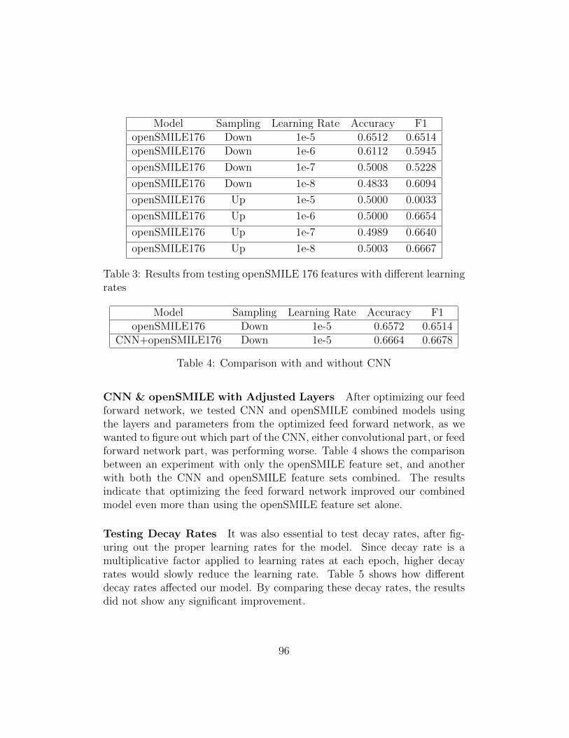
Model Sampling Learning Rate Accuracy F1openSMILE176 Down 1e-5 0.6512 0.6514openSMILE176 Down 1e-6 0.6112 0.5945

openSMILE176 Down 1e-7 0.5008 0.5228

openSMILE176 Down 1e-8 0.4833 0.6094

openSMILE176 Up 1e-5 0.5000 0.0033

openSMILE176 Up 1e-6 0.5000 0.6654

openSMILE176 Up 1e-7 0.4989 0.6640

openSMILE176 Up 1e-8 0.5003 0.6667

Table 3: Results from testing openSMILE 176 features with different learningrates

Model Sampling Learning Rate Accuracy F1openSMILE176 Down 1e-5 0.6572 0.6514

CNN+openSMILE176 Down 1e-5 0.6664 0.6678

Table 4: Comparison with and without CNN

CNN & openSMILE with Adjusted Layers After optimizing our feedforward network, we tested CNN and openSMILE combined models usingthe layers and parameters from the optimized feed forward network, as wewanted to figure out which part of the CNN, either convolutional part, or feedforward network part, was performing worse. Table 4 shows the comparisonbetween an experiment with only the openSMILE feature set, and anotherwith both the CNN and openSMILE feature sets combined. The resultsindicate that optimizing the feed forward network improved our combinedmodel even more than using the openSMILE feature set alone.

Testing Decay Rates It was also essential to test decay rates, after fig-uring out the proper learning rates for the model. Since decay rate is amultiplicative factor applied to learning rates at each epoch, higher decayrates would slowly reduce the learning rate. Table 5 shows how differentdecay rates affected our model. By comparing these decay rates, the resultsdid not show any significant improvement.

96

Model Sampling Learning Rate Decay Accuracy F1CNN+openSMILE176 Down 1e-5 0.6 0.6513 0.6499CNN+openSMILE176 Down 1e-5 0.7 0.6519 0.6471CNN+openSMILE176 Down 1e-5 0.8 0.6664 0.6678CNN+openSMILE176 Down 1e-5 0.9 0.6488 0.6209

Table 5: Comparison of Different Decay Rates

After all of these experiments, we saw a lot of improvements in accuracyand F1 score. We were able to achieve an accuracy and F1 score of 0.65above. This can be seen in Figure 82, which shows that accuracy curveand F1 score curve eventually rose. Train loss and test loss also convergedeventually. The amounts of True Positive went up and True Negative wentdown till they converge. These plots indicate that our model was learningand predicting well, but it was still far from perfect. Moreover, since we hadworked with our own generated folds for experiments, we had yet to see howour model would perform on official DAIC-WOZ folds.

97

(a) F1-score against epochs(b) True Positive/True Negativeagainst epochs

(c) Accuracy against epochs (d) Loss against epochs

Figure 82: Best Results from running CNN with openSMILE176

CNN & openSMILE with Adjusted Parameters and DAIC-WOZOfficial Splits Since we had been testing on our own random folds with70:30 splits, our results were not directly comparable with other researches.DAIC-WOZ data set had its own official train and test split. Thus, we testedour adjusted parameters again with the official train and test split. The table6 shows the results from testing with DAIC-WOZ official splits. As we cansee, the models did not perform as good as they did on random folds. Thehighest F1 score we could achieve was 0.5506 with respective accuracy of0.5811. From the research by Chen et al. (Ma et al., 2016), DepAudioNetcould achieve 0.52 F1 score. One reason why our models did not performwell on official splits was that, the official splits is grouped by participantsand not by audio clips. Thus, this created a different split ratio when were-grouped the official splits by audio clip.

98

Model Sampling Learning Rate Decay Accuracy F1CNN+openSMILE176 Down 1e-5 0.2 0.5488 0.5147CNN+openSMILE176 Down 1e-5 0.5 0.5149 0.4841CNN+openSMILE176 Down 1e-5 0.8 0.5041 0.4647CNN+openSMILE176 Down 1e-6 0.2 0.5811 0.5506CNN+openSMILE176 Down 1e-6 0.5 0.5232 0.5232CNN+openSMILE176 Down 1e-6 0.8 0.4909 0.5028

DepAudioNet 0.52

Table 6: Results from testing with DAIC-WOZ official splits

5.2.3 DAIC-WOZ: Sequential Model

Experiments were run on a model made using PyTorch as described inSections 4.2.2 and 4.2.3. Batch size and output dimension were 1, while theoptimizer type, learning rate, number of hidden nodes, number of layers, anddropout rate differed between experiments.

We first compared optimizer performance. We tried AdaDelta, RMSProp,and Adam with a learning rate of 1e-5, 128 hidden nodes, 1 layer, and nodropout. With these settings, we found that Adam performed the best, whichwas expected (see Figure 83). RMSProp performed slightly worse, howeverwas able to perform better with a very small learning rate and a small numberof hidden nodes. This will be discussed later. The model using Ada failedto learn anything with these hyperparamters and classified every example asnon-depressed. We continued to use Adam for the majority of experiments.Our next experiment was with learning rate. We found that a value of 1e-5was the most effective given the assumed 128 nodes and 1 layer.

99

(a) Adam model (b) Adam model

(c) RMSProp model (d) RMSProp model

(e) Metrics for each model. Actual TP/TN is 437/1632

Figure 83: A comparison of Adam vs RMSProp with a learning rate of 1e-5,128 nodes, and 1 layer

100

Random resampling of just the training set was introduced next. Becauseof the complexity of the input, random sampling made more sense than usingSMOTE. As each input was a variable-length sequence of lists, SMOTE wasmore difficult to implement. Continuing to use Adam with a learning rateof 1e-5, we ran a set of experiments on different combinations of {128, 256}hidden nodes, {0, 0.2, 0.4} dropout, and {1, 2, 3} layers. These modelsquickly showed training and testing loss diverging and a very high variancein accuracy and F1 between epochs. Overfitting increased with an increasein hidden nodes and layers. Higher dropout values appeared to hinder modellearning and, contrary to expectations, promote overfitting. This may beexplained by the relatively small data set and small majority class within(21% of the data set). Losing any of the tiny amount information predictingtrue positives could have been harmful to the model. Noticing the overfittingprompted us to experiment next on the number of hidden nodes.

Using Adam with a learning rate of 1e-5 and 1 layer, we tested {10, 30,50, 75, 100} hidden nodes. The results of these trials are shown in Figure84. As the number of nodes increased, we saw less divergence in train vs testloss and accuracy. There was also more variance in the curves. Accuracyincreased significantly, from roughly 0.5 with 10 nodes to around 0.65 with100 nodes. Loss also improved. However, as the nodes increased the modelbecame more overfit. With 10 nodes, the true positives were closest to theactual, but false positives were also the highest.

101

(a) 10 hidden nodes (b) 10 hidden nodes

(c) 50 hidden nodes (d) 50 hidden nodes

(e) 100 hidden nodes (f) 100 hidden nodes

102

Figure 84: A comparison of different hidden node amounts. Actual TP/TNis 437/1631.

The next set of experiments was done to determine if it was more effectiveto train with both the test and train sets upsampled, instead of just thetraining set. We also simultaneously ran experiments using the os25 featuresand the os176 features, testing upsampling test on both data sets. We foundthat the models performed far better when both test and training sets wereupsampled as shown in Figure 85. Both models were run using Adam witha 1e-5 learning rate, 128 nodes and 1 layer. Although the models both sufferfrom diverging loss and decreasing F1 score, they remain comparable. In Fig-ures 85c and 85d, the metrics point to worse than random with an accuracyof 0.45 and an F1 of 0.32. The untouched test set had 437 questions in theminority class (depressed) and 1631 in the majority. Random resampling ofthe minority class up to 1631 examples yielded better results. As seen in 85aand 85b, the overall fitness is better with an accuracy of 0.52 and an F1 of0.59. However, the test accuracy shows a decreasing trend, while the modelwith the untouched test set shows a fairly constant test accuracy.

Regarding the features, results were unclear at the beginning. We haveno direct comparisons between the os25 and os176 features, although wewitnessed a general trend towards better results and less overfitting in theconfusion matrices of models using the os176 features. We switched to usingthose for all remaining experiments.

103

(a) Both upsampled (b) Both upsampled

(c) Only test upsampled (d) Only test upsampled

Figure 85: A comparison of upsampling both train and test sets vs. just thetest set

After deciding to continue training models with the os176 feature set, weran a range of experiments with different combinations of learning rate andhidden nodes as shown in Figure 86. All experiments used the Adam op-timizer. These showed better results with smaller learning rates. Nodesbetween 200-250 appeared to perform the best, although the same trends asseen in the node size experiment were present. More nodes led to higher trueand false positives.

We then decided to test another hypothesis about the features. All previ-ous experiments has been using 3 second audio clips that overlapped by 75%.

104

Figure 86: Hyperparameters and metrics for models trained on os176 featuresusing Adam. Actual TP/TN is 1631/1631

Our hypothesis was that using the 3 second clips with no overlap could com-bat the overfitting that had been pervasive throughout our models. Unfortu-nately, the metrics showed our models performing slightly worse, averaginglower accuracy and F1. Both of the models in Figure 87 used 250 nodes and4 layers with a learning rate of 5e-7. One thing to note in the model trainedwith the 0 overlap features: Although F1 and recall trend upward and havenot settled, they are still far below that of the model trained on overlappingfeatures and probably would not have reached such high values regardless ofextra training.

105

(a) No overlap (b) No overlap

(c) 0.75 overlap (d) 0.75 overlap

(e)

Figure 87: A comparison of using 3 second Sub-Clips with no overlap and75% overlap between clips

106

In order to generate results comparable with other studies, we switchedover to using the official data splits from DAIC-WOZ. Because we were notusing a three-way split, the ’validation’ set was not used. This resulted ina training set around 60% instead of the previous 70%. All the data inthe ’validation’ set was not used, reducing the overall total amount of data.Random resampling was still used to upsample both the train and test sets.

At this point, we had trained most recent models with around 200 hiddennodes and a learning rate around 1e-6, and between 1 and 4 layers. Givenour past experimentation, these appeared to be close to the optimal hyper-parameters. We trained models with these settings on the previously definedsplit and got a mix of complete overfitting (all examples classified in ma-jority class) and other odd results that did not show learning. Given thatthe size of the data set was significantly smaller, we hypothesized that thehyperparamters and other settings were no longer optimal.

In response, we decided to test models with a smaller node count and learn-ing rate. With these hyperparameters, using the Adam optimizer tended toshow less learning, and could even fail to predict anything in the targetclass. We had previously noticed that RMSProp performance would slightlyincrease with lower node counts and learning rates, so we switched to RM-SProp for these experiments. Two experiments were run with 75 hiddennodes, 1 layer and a learning rate of 1e-7, with dropout rates of 0 and 0.5.Both models showed diverging train and test losses. Although F1 was trend-ing upwards, precision was constant and only recall was increasing. This isindicative of overfitting as well, as a higher recall can mean more false pos-itives. The same model with 75 hidden nodes and 1 layer was run with alearning rate of 1e-8 and showed very promising metrics. This was one ofthe first experiments in which we were able to see both train and test lossdecrease. It is not quite optimal, however, as the loss curves appear rela-tively linear with different slopes. Although test loss decreases, it will neverconverge with the train loss as the difference increases over time. Becausetrain and test accuracy, as well as both precision and recall, increased overtime and had not yet stabilized, we continued to train the model. Originallybeing trained for only 200 epochs, we trained for an additional 400 epochs.This model was able to achieve an accuracy of 0.51 with an F1 score of 0.56,recall of 0.63, and precision of 0.51.

107

The best sequence models come from a few different areas of experimen-tation. Our best model trained on the DAIC-WOZ split, although lackingin numbers compared to some others below, is the best that shows test setloss decreasing over time. Although all others show a divergence of trainand test loss over time, the models themselves are fit quite well to the dataand can provide classification significantly better than random. All followingmodels (excluding baselines) were trained on the os176 openSMILE featureset of the three second 75% overlap clips of DAIC-WOZ audio, using randomresampling to up-sample both train and test sets as described above. In the“Split” column of Figure 88, “Internal” refers to the sequential 70/30 splitand “ DAIC” refers to the official DAIC-WOZ split, both as described earlierin this section.

5.3 Topological Data Analysis

Data Set Model DR Features F1 Accuracy AUCULBC, First 5 XG3 Chi2 100 0.59 0.60 0.59SLBC, First 5 NB PCA 13 0.62 0.54 0.55

ULBC, Random 5 XG2 PCA 10 0.59 0.57 0.55SLBC, Random 5 NB PCA 10 0.60 0.56 0.54ULBC, First Clip XG4 Chi2 100 0.55 0.55 0.55SLBC, First Clip NB kPCA 11 0.55 0.53 0.54

OS176 + ULBC First 5 XG3 Chi2 80 0.70 0.69 0.72OS176 + SLBC First 5 XG3 Chi2 90 0.71 0.71 0.75

OS176 XG4 Chi2 90 0.71 0.70 0.75

Table 7: Results From Best Experiments. A PHQ-8 Score cutoff of 10 wasused for all tests. ULBC stands for Upper Level Betti Curve, SLBC standsfor Lower Level Betti Curve, OS Stands for openSMILE, and DR stands forDimensionality Reduction.

108

109

Figure 88: Our best LSTM-based sequence models over the course of thisproject, compared to baselines

110

For our data sets, we only used 5 second clips with no overlap. Acrossthe board, we found the best results with Betti curves when using NaiveBayes or XGBoost for models. These models consistently performed betterthan random for the majority of data. Our best results for Betti curveson their own were found when using the first 5 clips from each participant,versus random 5 or the first clip from each question. When using the firstclip from each question, our best results actually may be outliers, with mostresults lying close to random or worse. This may be due to the fact that thefirst couple clips from each participants are generally answering very similarquestions from the interviewer, which may prompt similar responses acrossparticipants. Sub level Betti curves provided better results than upper levelBetti curves in some scenarios, usually with a Naive Bayes model. Whencombined with the openSMILE 176 feature set, much better results werefound with both upper level and sub level Betti curves. It is somewhatdoubtful that the Betti curve features are actually being used in these resultshowever, as PCA was applied and the openSMILE features on their ownperformed extremely similarly.

5.4 Generative Adversarial Networks

5.4.1 ACE Experiments

These experiments were run after Texygen was first set up on the ACEcluster. These are the following parameters for these experiments:

Parameter ValueTotal Epochs 50

Pre-Training Epochs 20Adversarial Training Epochs 30

Input Texts 1074

Though RankGAN had a higher average BLEU score, all of the BLEUscores from this experiment were exceptionally low. We hypothesise thatthis was due to the inconsistent nature of text data, so the GANs were notable to find consistent patterns from the texts to recreate. The number ofepochs was also reduced, from the 80 pre-training and 100 adversarial trainingepochs, used in previous studies, to only 20 pre-training and 30 adversarialtraining epochs, due to the limitations of the ACE cluster.

111

Figure 89: Comparison of BLEU-4 Scores: ACE Experiments

GAN Method Average BLEU-4 ScoreMLE 0.001950947597504571

SeqGAN 0.0015532267864985627RankGAN 0.0043830571838256085LeakGAN 0.002125034325184055

112

Figure 90: NLL-test Loss Over 50 Epochs

The NLL-test loss in Figure 90 shows that it did not converge, nor did itgo notably low for LeakGAN or RankGAN. Once again, this was expected,due to the low number of epochs run from this current experiment. Despitethe very low results compared to the studies that implemented these GANmethods, we can consider this phase of experiments a success, due to showingthat these GAN methods can successfully be run on our SMS message data.

5.4.2 Turing Experiments

The second round of experiments performed on the Turing cluster wasmore to prove the functionality of the improved framework than to test theviability of individual text generation methods. The following parameterswere used for the experiments on Turing:

Parameter ValueTotal Epochs 60

Pre-Training Epochs 30Adversarial Training Epochs 30

Input Texts 2000Each of these SMS texts was from a single participant, and no word

frequency filtering or filtering by length was done. A distribution of BLEU

113

scores among Sequence GAN methods run on Turing can be seen in Figure92:

Figure 91: Comparison of BLEU-4 Scores: Turing Experiments

GAN Method Average BLEU-4 ScoreMLE 4.126752767215812e-156

SeqGAN 0.010481158991399186RankGAN 0.012939276614873981LeakGAN 0.09086621413976959

These experiments all finished within twelve hours, despite having moreepochs, due to the increased resources of the Turing cluster. As a result ofthe increased number of epochs, methods had average BLEU-4 scores a fullexponent greater than the previous experiments. LeakGAN’s average BLEUscore are considerably worse, due to LeakGAN having a bug and crashingafter fifteen epochs. Unusually, MLE performed considerably worse than theprevious tests, presumably due to running only the thirty pre-training epochs

114

instead of the full sixty.

Figure 92: Comparison of NLL-Test Scores: Turing Experiments

Figure 92 shows the NLL-test loss scores over all sixty epochs of this roundof experiments. MLE and LeakGAN NLL-test loss scores are not displayedhere due to output issues with both methods. As seen in the previous roundof experiments, NLL-test loss fell rapidly during pre-training, and slowly roseback up

6 Conclusion

Overall, we have been able to reliably demonstrate the ability of our im-plemented machine learning and deep learning methods to detect depression

115

and anxiety using voice audio and accompanying transcripts. This technol-ogy could open new opportunities for how patients of depression or anxietyare treated. It could also help many who lack access to mental health re-sources or who are undiagnosed find the help they need. Reliable detectionof depression can also be used in sentiment analysis. The ethical concernsof this are significant and the technology can easily be abused. All neces-sary precautions should be taken to ensure that private or government use ofthis type of depression detection is monitored and ethical in order to avoidanother study like (Kramer et al., 2014), in which almost 700,000 Facebookusers were emotionally manipulated without consent.

In Machine Learning scope of research, we have seen that SCB has im-proved our prediction results. Using regression hasn’t altered our resultssignificantly. We were also able to perform slightly better when detectinganxiety through GAD-7 labels. In addition, tree based ensemble methodslike XGB and ADA have performed better overall. Future improvements canbe made by adding feature selection methods like PCA, Chi2, etc. SVMscould also be used with Gaussian kernel, polynomial kernel, and Sigmoidkernels to improve predictions (Valstar et al., 2016). Using CNN for detect-ing depression has proven to be effective as we were able to achieve an F1score close to DepAudioNet’s. Some of the models we tested on random foldswere able to perform better. Another step to continue improving this modelwould be adjusting our input to be grouped by participants instead of audioclips. Using LSTM-based sequence models has also proven effective, reachingan F1 score of as high as 0.68. Different data processing can be implementedto improve results further, but training a sequence model with both audioand the respective transcript is the most promising path forward. A largerdata set would also be impactful. Using Betti Curves with topological dataanalysis has been shown to provide better than random results. SequenceGAN methods have been fully set up to experiment with artificial participantgeneration in future studies.

6.1 Machine Learning

We started out this research by experimenting with Machine Learningmethods on DAIC-WOZ data set. Initial phase of experimentation didn’tinclude grid search, up-sampling, and ADA method. In addition, we were

116

using only Praat features due to computational restrictions - research ex-periments were mainly conducted locally at this point. No GAD-7 basedexperiments were also done during this phase. SCB and Regression weren’tintegrated into our Machine Learning pipeline as well. As a result, our ex-periments weren’t fruitful and we obtained a highest F1 score of 0.63 andscores ranged between 0.48 - 0.63.

We were able to move our experiments to ACE cluster. This enabled usto compute more experiments and do computationally expensive tests. Westarted using openSMILE features, added regression approach to all methodswe had been using, started sub-clip boosting, expanded dataset. These led tobetter overall results. Specifically, up-sampling, SCB, openSMILE featuresall improved our model’s performance significantly. We also found our overallbest results when using EMU dataset with GAD-7 labels: highest result wasa test run with an XGB method using a cutoff of 5 which resulted in a F1score of 0.828. We also outperformed previous MQP’s EMU audio feature testresults; they produced a highest F1 score of 0.7, while we were able to reachup to a F1 score of 0.813. Our pipeline didn’t perform well with DAIC-WOZwhen using official train and test split. The highest F1 score for this sectionof experiments was 0.513. This could be to not using other feature selectiontechniques: we used only one type of feature selection approach outlined insection 4.1.2. In addition, we also weren’t able to use SVM unless we setthe kernel to linear. Other related works have generated higher results usingSVMs with other kernels (Valstar et al., 2016).

6.2 Deep Learning

Since we already have the EMU and Moodable data sets available fromprevious MQP, we used it to implement our first deep learning pipeline whilewe figured out the data-preprocessing for DAIC-WOZ data set. Runningfirst on EMU and Moodable data sets was not able to give us good resultsbut it gave us a foundation of knowledge in deep learning aspect of detectingdepression. When all the data were prepared ready for DAIC-WOZ data set,we started our process of finding an efficient model which will help predictdepression.

117

Neural Networks We started off testing with a base model and changedone step at a time to see any noticeable difference. Through testing differentlayers, kernel sizes, combination of feature sets, learning rates and decays,our final model was able to achieve a F1 score of above 0.6678 with accuracyof 0.6664 on random folds. Then, we tested this model with official foldsto compare against DepAudioNet (Ma et al., 2016). With Official folds, ourmodel barely performs as good as DepAudioNet since our model achieveda F1 score of 0.5506 whereas the best result of DepAudioNet is 0.52. Test-ing with random folds and testing with official folds give us a significantlydifferent F1 scores while the former performs better than the latter. Ourconclusion on this difference of F1 scores is that we were using the splitswhich were grouped by audio clips instead of participants although a singleparticipant was not cross-included in both of train and test set. The officialsplits were grouped by participants and when we re-grouped them into audioclips, we have different ratio splits.

Since the features extracted from audio play a huge part in finding anefficient model, combining convoluted feature sets with other feature setssuch as PRAAT or Betti curves could produce potential results. Anotherapproach to improve our model would be using multimodal approach. Inthis approach, not only audio data but also other available data such astext messages and transcripts should be considered for feeding into each sub-network (which could a be CNN or LSTM).

Sequence Model Using LSTM-based neural networks has proved an effec-tive method for categorical depression prediction using voice samples alone.Our best model was able to show an F1 of 0.68, precision of 0.55, recall of0.91, and accuracy of 0.58. As compared to the best baseline (Al Hanai et al.,2018), we have +0.05 F1, -0.16 precision, and +0.35 recall. However, there isstill room for improvement. All of our models suffered from overfitting. Thisis most likely because of the size of the data set. Sequence models typicallyperform better when they are fed a large and diverse data set, and DAIC-WOZ may simply not be expansive enough. Other studies (Al Hanai et al.,2018) have addressed this issue by training two parallel sequence models, onetrained on audio data and the other on the transcripts of the same audio.Combining their output has shown to significantly increase accuracy and F1score.

118

Using larger data set opens up some more possibilities for data prepara-tion. At one point, we removed all inputs from the LSTM training data thathad a size of 1, i.e. removed all inputs where the question response was onlyone clip long. This reduced the data set by too much and exasperated theissues we experienced that were caused by small data set size. This techniquecould be applied to a far larger data set for more accurate results.

Additionally, making the model bidirectional allows it to consider relevant’memory’ generated from both past and future events in the sequence. Thisadditional context could reduce the number of false positives. The benefitsof this will be compounded when using a larger data set. Another interestingpossibility is using raw spectrogram data, instead of features, as input for theLSTM model. Slices of a Sub-Clip’s spectrogram can be treated sequentially.

Compared to other attempts to use sequence modelling with DAIC-WOZaudio, our models tend to perform as well, if not better in many cases(Al Hanai et al., 2018). We believe that combining our current model witha model trained on transcript data would significantly improve performance,possibly exceeding an F1 score of 0.8. As shown in Al Hanai et al. (2018),their multimodal model demonstrates an increase of +0.14 in F1 and +0.27in recall over their model trained on just audio.

Another technique to implement could be the SMOTE algorithm. Ran-dom resampling had been used to upsample the minority class for many ofthe experiments. But it can still promote overfitting with it’s inability toproduce new data. Random resampling could still be used to generate moreinstances of the depressed class, but inside each resampled input sequence,SMOTE can be applied to replace the sequences of features with new gener-ated arrays. Synthetically expanding the amount of unique data may lead toimprovements on many of the issues outlined with our sequence modelling.

6.3 Topological Data Analysis

Our main goal with using Topological Data Analysis was to determineif Betti curves generated from sound waves are viable in machine learning.Betti curves, as stated in Section 2.10.5, are a general method for interpretingpersistence barcodes as data. However, our construction of a filtered complexwas unique (Section 4.5) and was only previously used in a study which used

119

Betti curve to analyze heart beats to categorize heart arrhythmias (Dindinet al., 2019). From our results, we can see that Betti curves were indeedable to provide useful information, such that our models produced betterthan random results. When combined with a known good form of featureextraction, openSMILE, even better results were found. However, it seemsthat the openSMILE features may be responsible for the majority of thesegood results. Regardless, our goal was to determine if Betti curves wereviable at all as a form of feature extraction on sound waves, and we concludethat they are.

Several things can easily be done for future work on this topic. For one,varying clip lengths and looking at overlapping clips would be a good idea,as this could determine what length of clips work best with Betti curves.Overlap on waves was used in a previous study using Betti curves as well(Dindin et al., 2019), so better results may be found using this method. Usinga larger data set may provide better results as well, as we used a truncateddata set in all of our testing due to the limitations of our cluster computing.Using Betti curves as a feature in deep learning would be an interestingavenue to approach as well, as previous studies used this approach (Dindinet al., 2019).

6.4 Generative Adversarial Networks

The goal of this branch of the project was more to develop an environment forfuture studies than to show the feasibility of any particular text generationmethod. One clear conclusion that can be drawn, however, is that the dataset we have been using for testing text generation is very inconsistent and dif-ficult to train a sequence GAN with. Other studies that used sequence GANmethods filtered their data sets to texts that are all around the same length(Nie et al., 2019). This allows the GAN to learn a smaller number of extrafeatures and generate more consistent texts. As a result, we suspect thattext data sets of a more consistent length, such as Twitter messages, wouldwork considerably better for generating consistent new data with sequenceGANs.

Despite our best efforts, there were some definite limitations of our ex-periments with sequence GANs. LeakGAN has been problematic since thevery beginning, and despite multiple attempts to debug it, we could not getit to run more than 15 epochs, so we do not have complete data on it.

120

The framework we have built for testing sequence GAN methods will beuseful for future studies to test the feasibility of artificial participant gener-ation. This can be proven by selecting SMS messages from real participantswith similar PHQ-8 scores, and generating an artificial participant with theirdata. If the deep learning or machine learning method can correctly classifythe new participant, then the feasibility of artificial participant generationwill have been proven. Furthermore, it would be highly beneficial for futurestudies to standardize the output files from each GAN method in Texygen, toallow for much easier comparing of GAN methods. The output files used forthis round of experiments still required manual reformatting to allow themto be plotted against each other.

A Tables of Accomplishments

A.1 A Term

Name Accomplishments

Nick

Team LeaderSet up communication logisticsDownloaded/Organized DAIC-WOZWrote initial DAIC-WOZ audio processing codeDepression and machine learning lit reviewWrote report outlineMajor report editor

Adam

Team ScribeLiterature review on DAIC-WOZDAIC-WOZ Audio Processing: Slicing into questions and X-second segments, organizationDAIC-WOZ Audio Processing StatisticsMental Health + Patient Health Questionnaire Literature ReviewSet up LaTex Document and Bibtex CitationsMinor editing in reportWrote Sections on DAIC-WOZ, Patient Health Questionnaire,Depression Statistics, and Data Processing

Myo

Deep Learning specifically CNN, and RNNSet up clusters and Python environments for team membersResearched suitable Frameworks to build Neural NetworksBuilt and experiment CNN models using Pytorch and Python

121

Name Accomplishments

Joe

Set up Git repositoryResearched different types of neural networks to determine best fit for our taskResearched different ways to format audio data to feed into a neural netResearched how to evaluate deep learning modelsLearned how to Jupyter and research clusterStarted to experiment with CNN model, testing different hyperparamters with EMU and DAICLearned LaTeX, Python, and PyTorchLent lots of assistance to group members with Git issues

Yosias

Made the following modifications to analyzer script with Yared:including regression,fixing train/test method,generating predictions,worked on script to make it run through different parameters,worked on getting it to run on the cluster.Did audio slicing for 3-7 seconds on local machine and for overlap.Did Praat and openSMILE extraction for 3-7 seconds DIAC-WOZ on local machineWorked with Yared to modify openSMILE to make it work on cluster.Worked with Joe to make Praat work on cluster.

Yared

DAIC-WOZ slices organization Appended PHQ-8 ScoresLiterature Review on Data Balancing and Evaluation ModelsResearched Metrics (Confusion Matrix, F1, precision, recall)Further processed audio slices for pratt extraction compatibilityRun initial experimental tests in Machine Learning modelsAnalysis of test resultsWrote XGBoost, Random Forest and Decision Tree and Artificial Neural NetworksWrote Data Balancing SectionWrote Evaluation Metrics

122

A.2 B Term

Name Accomplishments

Nick

Sequence GAN sub-projectSet up TexygenDebugged TexygenProcessed Moodable text dataRan SeqGAN experimentsWrote code to process experiment resultsMajor editor for the reportFixed bibliography errors

Adam

Developed code for generating topological data from sound wavesCreated data set of DAIC-WOZ 5 second Betti curvesPerformed in-depth research on TDAResearch on PCA and NMFWrote sections on dimensionality reduction techniquesWrote TDA background sectionWrote TDA implementation sectionWrote TDA AnalysisHelped debug LaTex codeAdded new DAIC-WOZ boxplots

Myo

Deep Learning specifically CNN, and RNNSet up clusters and Python environments for team membersResearched suitable Frameworks to build Neural NetworksBuilt and experiment CNN models using Pytorch and PythonReduced Training time by image cachingAdded Up-sampling on DAIC-WOZ dataImplemented experiments regarding to kernel sizes and layers

123

Name Accomplishments

Joe

Created and implemented an LSTM model in PyTorch and experimented heavily ondata sources and formats, hyperparameters, internal settings, sampling techniquesAttempted an LSTM model with spectrogram inputImplemented LSTM model in Keras based on paper, experimentedwith our data (mostly learning experience, recorded on weekly slides but no results in paper)Continued experimentation on CNN with DAIC, including learning rate decayResearched ways to combine audio and text inputsInitiated and followed through on managing use and access oflarge data sets in Git and on the research clusterCreated starter documents for DL and ML testing workflows and Git usageWrote script framework for managing LSTM experiment submission and loggingStarted an experiments log with a suite of robust performance analysis toolsModified Praat feature generation script, wrote wrappers for feature extraction job managementAssisted with Praat section in instruction manualLent lots of assistance to group members with Git issues

Yosias

Made the following modifications to analayzer script with Yared:including regression,fixing train/test method,generating predictions,worked on script to make it run through different parameters,worked on getting it to run on the cluster.Did audio slicing for 3-7 seconds on local machine and for overlap.Did Praat and openSMILE extraction for 3-7 seconds DIAC-WOZ on local machineWorked with Yared to modify openSMILE to make it work on cluster.Worked with Joe to make Praat work on cluster.

Yared

Organize Test/Train sets and setIncluded Regression Models and added model parameter optionsAdded prediction outputs for sub-clipsRan experiments for Classification models over multiple variationsStart setting up Machine Learning pipeline on clusterWrote Machine learning results and methods (with Yosias)Worked with Ermal for incorporating Machine Learning process on clusteropenSMILE feature generation for all sub-clip variations on EMUSet up instruction manual and organized the outlineWas scribe for the termUpload all data to a workspace on Ace clusterWrote script to determine number of features to use

124

A.3 C Term

Name Accomplishments

Nick

Sequence GAN Sub-ProjectDebugged TexygenModified Texygen with parameter argumentsGot RelGAN workingModified RelGAN to accept other data setsMade Texygen job file generatorMade RelGAN job file generatorRan Texygen and RelGAN experimentsWrote code to process experiment resultsRe-organized reportEdited every section in the reportWrote all Generative Adversarial Network sections

Adam

Rewrote and expanded all TDA sectionsIn depth research into topology and persistent homology216+ unique machine learning experiments with Betti curvesGenerated all truncated Betti curve data setsGenerated combined openSMILE/Betti curve data setsModified code for running batch machine learning experimentsWrote code for truncated and combined data set generationDebugged LaTeXAdded design improvements to report

Myo

Deep Learning specifically CNN, and RNNTeam LeaderBuilt and experiment CNN models using Pytorch and PythonDeveloped code for multiple deep learning models, andcombining CNN with openSMILETested various hyperparameters for CNNAdded Upsampling and Downsampling on DAIC-WOZ data

125

Name Accomplishments

Joe

Continued expansive experimentation on main LSTM modelBrief experimentation on Keras LSTM model for binary classificationHeavily expanded on logging and performance analysis/visualization tools to include moreautomated data collection and higher quality/more flexible visualizationsSignificant time and effort debugging PyTorch, issues on Ace clusterSquashed bugs in the Praat feature generation pipelineFocused lots of work on the final reportResearched adding CNN layers for feature extraction on top of LSTMLent lots of assistance to group members with Git issuesServed as scribe for the term

Yosias

Worked on the Transcript component of DAIC-WOZDid pre-processing work on transcripts and set up scripts for itWorked on modifying text extraction code to function for DAIC-WOZ transcriptsExtracted Textblob and Empath featuresWorked on doing tests for transcript and audio features combinedworked on setting up pipeline for transcript +audio

Yared

Continue and finalize regression experimentsFinalize EMU, Moodable and DAIC-WOZ dataset experimentsIncorporate GAD into Machine Learning experiment scopeTested SCB with audio filesGenerate Official DAIC-WOZ foldsGenerate in-team DAIC WOZ foldResearch GAD-7 anxiety background and related worksWrote Machine Learning Methods (section 4.1)Wrote Machine Learning Results (section 5.1.1, 5.1.2, 5.1.3 and, 5.1.4)GAD-7 vs PHQ-8 analysisSCB impact analysisCode debugging and assisting teammates in using Machine Learning pipeline

126

B Table of Authorship

Section Primary Author Primary EditorAbstract Joe, Nicolas Joe1: Introduction Nicolas, Adam Joe1.1: Related Works All Joe1.2 Our Approach All Joe2.1: Previous MQPs Yosias2.2: Depression Statistics Adam, Yared2.3: Data Sources Adam, Yosias2.4: Dimensionality Reduction Techniques Adam2.5: Data Balancing Yared2.6: Evaluation Metrics Yared Joe, Adam2.7: Machine Learning Yared, Yosias Yared2.8: Deep Learning Myo, Joe Joe, Adam2.9: Machine Learning and Deep Learning Frameworks Myo Joe2.10: Topological Data Analysis Adam Nicolas2.11: Generative Adversarial Networks Nicolas Adam3.1: Text Feature Extraction for Machine Learning Yosias3.2: Audio Feature Extraction for Machine Learning Yosias3.3: Topological Data Analysis Adam Prof. Paffenroth3.4: Generative Adversarial Networks Nicolas Adam4.1: Machine Learning Yared, Yosias4.2: Deep Learning Myo, Joe Joe4.3: Tests Run on Audio Data Yosias4.4: Tests Run on Transcript Yosias4.5: Topological Data Analysis Adam Nicolas, Prof. Paffenroth4.6: Generative Adversarial Networks Nicolas Adam5.1: Machine Learning Yared, Yosias Yared5.2: Deep Learning Myo, Joe Joe, Adam5.3: Topological Data Analysis Adam Prof. Paffenroth5.4: General Adversarial Networks Nicolas Adam6: Conclusions Joe6.1: Machine Learning Yared, Yosias6.2: Deep Learning Myo, Joe Joe6.3: Topological Data Analysis Adam Nicolas, Prof. Paffenroth6.4: General Adversarial Networks Nicolas

127

References

Abu-Rmileh, A. (2019). The multiple faces of ‘feature impor-tance’ in xgboost. https://towardsdatascience.com/be-careful

-when-interpreting-your-features-importance-in-xgboost

-6e16132588e7.

Ahire (2018). The artificial neural networks handbook: Part 1.

Al Hanai, T., Ghassemi, M., and Glass, J. (2018). Detecting depression withaudio/text sequence modeling of interviews. In Proc. Interspeech 2018,pages 1716–1720.

Al Hanai, T., Ghassemi, M. M., and Glass, J. R. (2018). Detecting depressionwith audio/text sequence modeling of interviews. In Interspeech, pages1716–1720.

Alghowinem, S., Goecke, R., Wagner, M., Epps, J., Breakspear, M., andParker, G. (2013). Detecting depression: a comparison between sponta-neous and read speech. In 2013 IEEE International Conference on Acous-tics, Speech and Signal Processing, pages 7547–7551. IEEE.

Ali, A. (2018). K-nearest neighbor with practical implementa-tion. https://medium.com/machine-learning-researcher/k-nearest

-neighbors-in-machine-learning-e794014abd2a.

Anderson, M. (2019). Mobile technology and home broadband 2019. PewResearch Center: Internet, Science & Tech.

Banerjee, S. (2018). An introduction to recurrent neural networks.

Batista, G., Prati, R., and Monard, M.-C. (2004). A study of the behaviorof several methods for balancing machine learning training data. SIGKDDExplorations, 6:20–29.

Berry, E., Chen, Y.-C., Cisewski-Kehe, J., and Fasy, B. T. (2018). Functionalsummaries of persistence diagrams. arXiv preprint arXiv:1804.01618.

Bhumika Gupta, Akshay Jain, N. D. A. R. A. A. (2017). Analysis of variousdecision tree algorithms for classification in data mining.

128

Binieli, M. (2018). Machine learning: an introduction to mean squared er-ror and regression lines. https://www.freecodecamp.org/news/machine-learning-mean-squared-error-regression-line-c7dde9a26b93/.

Boissonnat, J.-D. and Maria, C. (2014). The simplex tree: An efficient datastructure for general simplicial complexes. Algorithmica, 70(3):406–427.

Brems, M. (2019). A one-stop shop for principal componentanalysis. https://towardsdatascience.com/a-one-stop-shop-for

-principal-component-analysis-5582fb7e0a9c.

Brid, R. S. (2018). Decision trees–a simple way to visualize a deci-sion. https://medium.com/greyatom/decision-trees-a-simple-way

-to-visualize-a-decision-dc506a403aeb.

Brownlee, J. (2019). Understand the impact of learning rate on neu-ral network performance. https://machinelearningmastery.com/

understand-the-dynamics-of-learning-rate-on-deep-learning

-neural-networks/.

Bubenik, P. (2017). Introduction to topological data analysis.

Buitinck, L., Louppe, G., Blondel, M., Pedregosa, F., Mueller, A., Grisel,O., Niculae, V., Prettenhofer, P., Gramfort, A., Grobler, J., Layton, R.,VanderPlas, J., Joly, A., Holt, B., and Varoquaux, G. (2013). API designfor machine learning software: experiences from the scikit-learn project.In ECML PKDD Workshop: Languages for Data Mining and MachineLearning, pages 108–122.

Carlsson, G. (2009). Topology and data. Bulletin of the American Mathe-matical Society, 46(2):255–308.

Chawla, Bowyer, H. K. (2002). Smote: Synthetic minority over-samplingtechnique. AI Access Foundation and Morgan Kaufmann Publishers.

Chepushtanova, S., Emerson, T., Hanson, E. M., Kirby, M., Motta, F. C.,Neville, R., Peterson, C., Shipman, P. D., and Ziegelmeier, L. (2015).Persistence images: An alternative persistent homology representation.CoRR, abs/1507.06217.

Darji, H. (2019). An approach to solve the bird counting problem.

129

Demir, N. (2015). Ensemble methods: Elegant techniques to produceimproved machine learning results. https://www.toptal.com/machine

-learning/ensemble-methods-machine-learning.

Dham, S., Sharma, A., and Dhall, A. (2017). Depression scale recognitionfrom audio, visual and text analysis. CoRR, abs/1709.05865.

Dindin, M., Umeda, Y., and Chazal, F. (2019). Topological Data Analysisfor Arrhythmia Detection through Modular Neural Networks. 7 pages, 4figures.

Dogrucu, A., Perucic, A., Isaro, A., and Ball, D. (2018). Sensing depression.

Drakos, G. (2018). How to select the right evaluation metric for machinelearning models: Part 1 regression metrics. https://towardsdatascience.com/how-to-select-the-right-evaluation-metric-for-machine

-learning-models-part-1-regrression-metrics-3606e25beae0.

Edelsbrunner, H. and Harer, J. (2008). Persistent homology-a survey. Con-temporary mathematics, 453:257–282.

Fast, E., Chen, B., and Bernstein, M. S. (2016). Empath. Proceedings of the2016 CHI Conference on Human Factors in Computing Systems.

Flach, P. A. (2003). The geometry of roc space: Understanding machinelearning metrics through roc isometrics. https://www.aaai.org/Papers/ICML/2003/ICML03-028.pdf.

Fortuner, B. (2017). Logistic regression. https://ml-cheatsheet

.readthedocs.io/en/latest/logistic regression.html.

Furr, S. R., Westefeld, J. S., McConnell, G. N., and Jenkins, J. M. (2001).Suicide and depression among college students: A decade later. Profes-sional Psychology: Research and Practice, 32(1):97–100.

Gandhi, R. (2018). Support vector machine — introduction to ma-chine learning algorithms. https://towardsdatascience.com/

support-vector-machine-introduction-to-machine-learning

-algorithms-934a444fca47.

Ghrist, R. (2008). Barcodes: the persistent topology of data. Bulletin of theAmerican Mathematical Society, 45(1):61–75.

130

Gong, Y. and Poellabauer, C. (2018). How do deep convolutional neuralnetworks learn from raw audio waveforms?

Goodfellow, I., Pouget-Abadie, J., Mirza, M., Xu, B., Warde-Farley, D.,Ozair, S., Courville, A., and Bengio, Y. (2014). Generative adversarialnets. In Ghahramani, Z., Welling, M., Cortes, C., Lawrence, N. D., andWeinberger, K. Q., editors, Advances in Neural Information ProcessingSystems 27, pages 2672–2680. Curran Associates, Inc.

Guillaume Lemaˆıtre, Fernando Nogueira, C. K. A. (2017). Imbalanced-learn: A python toolbox to tackle the curse of imbalanced datasets inmachine learning.

Guntuku, S. C., Yaden, D. B., Kern, M. L., Ungar, L. H., and Eichstaedt,J. C. (2017). Detecting depression and mental illness on social media: anintegrative review. Current Opinion in Behavioral Sciences, 18:43 – 49.Big data in the behavioural sciences.

Guo, J., Lu, S., Cai, H., Zhang, W., Yu, Y., and Wang, J. (2017). Longtext generation via adversarial training with leaked information. CoRR,abs/1709.08624.

Harrison, O. (2018). Machine learning basics with the k-nearest neigh-bors algorithm. https://towardsdatascience.com/machine-learning

-basics-with-the-k-nearest-neighbors-algorithm-6a6e71d01761.

Homans, Doosje, V. V. (2012). The validity of the phq-9 and the gad-7 forscreening depressive and anxiety disorders in sick-listed workers. Masterthesis Clinical and Health Psychology.

Hossin, M. and Sulaiman, M. (2015). A review on evaluation metrics for dataclassification evaluations. https://pdfs.semanticscholar.org/6174/

3124c2a4b4e550731ac39508c7d18e520979.pdf.

Hunt, J. and Eisenberg, D. (2010). Mental health problems and help-seekingbehavior among college students. Journal of Adolescent Health, 46(1):3 –10.

Kramer, A. D. I., Guillory, J. E., and Hancock, J. T. (2014). Experimentalevidence of massive-scale emotional contagion through social networks.Proceedings of the National Academy of Sciences, 111(24):8788–8790.

131

Kroenke, K., Spitzer, R. L., and Williams, J. B. (2001). The phq-9: validityof a brief depression severity measure. Journal of general internal medicine,16(9):606–613. 11556941[pmid].

Kroenke, K., Strine, T. W., Spitzer, R. L., Williams, J. B., Berry, J. T., andMokdad, A. H. (2009). The phq-8 as a measure of current depression inthe general population. Journal of Affective Disorders, 114(1):163 – 173.

Le Cun, Y., Denker, J. S., and Solla, S. A. (1990). Optimal brain damage.In Touretzky, D. S., editor, Advances in Neural Information ProcessingSystems 2, pages 598–605. Morgan-Kaufmann.

Li, H., Kadav, A., Durdanovic, I., Samet, H., and Graf, H. P. (2016). Pruningfilters for efficient convnets. CoRR, abs/1608.08710.

Librosa Development Team, L. (2019). librosa.decompose.decompose.https://librosa.github.io/librosa/generated/librosa.decompose

.decompose.html.

Lin, K., Li, D., He, X., Zhang, Z., and Sun, M. (2017). Adversarial rankingfor language generation. CoRR, abs/1705.11001.

Liu, J., Jeng, S., and Yang, Y. (2016). Applying topological persis-tence in convolutional neural network for music audio signals. CoRR,abs/1608.07373.

Loria, S. (2018). Textblob: Simplified text processing. https://textblob

.readthedocs.io/en/dev/index.html.

Ludena-Choez, J., Quispe-Soncco, R., and Gallardo-Antolın, A. (2017). Birdsound spectrogram decomposition through non-negative matrix factoriza-tion for the acoustic classification of bird species. PLOS ONE, 12(6):1–20.

Ma, X., Yang, H., Chen, Q., Huang, D., and Wang, Y. (2016). Depau-dionet: An efficient deep model for audio based depression classification.In Proceedings of the 6th International Workshop on Audio/Visual Emo-tion Challenge, AVEC ’16, pages 35–42, New York, NY, USA. ACM.

Mansar, Y. (2018). Audio classification : A convolutional neural net-work approach. https://medium.com/@CVxTz/audio-classification-a-convolutional-neural-network-approach-b0a4fce8f6c.

132

Marchese, A. (2017). Data analysis methods using persistence diagrams.University of Tennessee.

Marcus, M., Yasamy, M. T., Ommeren, M., Chisholm, D., and Saxena, S.(2012). Depression: A global public health concern. World Health Orga-nization Paper on Depression, pages 6–8.

Martınez-Trinidad, J. H. A. C.-O. F. (2013). An empirical study of over-sampling and undersampling for instance selection methods on imbalancedatasets.

Meryll, D. (2018). From topological data analysis to deep learning:No pain no gain. https://towardsdatascience.com/from-tda-to-dl

-d06f234f51d.

Molchanov, P., Tyree, S., Karras, T., Aila, T., and Kautz, J. (2016). Prun-ing convolutional neural networks for resource efficient transfer learning.CoRR, abs/1611.06440.

Monica Tlachac, E. R. (2020). Screening for depression with retrospectivelyharvested private versus public text. https://ieeexplore.ieee.org/

document/9049136/keywords.

Narkhede, S. (2018). Understanding auc - roc curve. https://

towardsdatascience.com/understanding-auc-roc-curve

-68b2303cc9c5.

Nguyen, M. (2018). Illustrated guide to lstm’s and gru’s: A step by step ex-planation. https://towardsdatascience.com/illustrated-guide-to

-lstms-and-gru-s-a-step-by-step-explanation-44e9eb85bf21.

Nie, W., Narodytska, N., and Patel, A. B. (2019). Relgan: Relational gener-ative adversarial networks for text generation. In ICLR.

Olah, C. (2015). Understanding lstm networks. https://colah.github.io/posts/2015-08-Understanding-LSTMs/.

Papineni, K., Roukos, S., Ward, T., and jing Zhu, W. (2002). Bleu: a methodfor automatic evaluation of machine translation. In Proceedings of the 40thAnnual Meeting of the Association for Computational Linguistics, pages311–318.

133

Piccinelli, M. and Wilkinson, G. (2000). Gender differences in depression:Critical review. British Journal of Psychiatry, 177(6):486–492.

Piczak, K. J. (2015). Environmental sound classification with convolutionalneural networks. In 2015 IEEE 25th International Workshop on MachineLearning for Signal Processing (MLSP). IEEE.

Raschka, S. (2015). Principal component analysis. http://

sebastianraschka.com/Articles/2015 pca in 3 steps.html, jour-nal=Dr. Sebastian Raschka.

Resnik, P., Armstrong, W., Claudino, L., Nguyen, T., Nguyen, V.-A., andBoyd-Graber, J. (2015). Beyond lda: Exploring supervised topic model-ing for depression-related language in twitter. In Proceedings of the 2ndWorkshop on Computational Linguistics and Clinical Psychology: FromLinguistic Signal to Clinical Reality, pages 99–107, Denver, Colorado. As-sociation for Computational Linguistics.

Resom, A., Assan, J., Flannery, M., Gao, Y., and Yuxin, W. (2019). Machinelearning for mental health detection.

Ringeval, F., Schuller, B., Valstar, M., Gratch, J., Cowie, R., Scherer, S.,Mozgai, S., Cummins, N., Schmitt, M., and Pantic, M. (2017). Avec 2017:Real-life depression, and affect recognition workshop and challenge. In Pro-ceedings of the 7th Annual Workshop on Audio/Visual Emotion Challenge,AVEC ’17, pages 3–9, New York, NY, USA. ACM.

Saha, S. (2018). A comprehensive guide to convolutional neural networks —the eli5 way. https://towardsdatascience.com/a-comprehensive-guide-to-convolutional-neural-networks-the-eli5-way-3bd2b1164a53.

Sayantini (2019). Keras vs tensorflow vs pytorch : Comparison of the deeplearning frameworks. https://www.edureka.co/blog/keras-vs-tensorflow-vs-pytorch/.

Shiruru, K. (2016). An introduction to artificial neural network. volume 1,pages 27–30.

Spitzer, R. L., Kroenke, K., Williams, J. B., and Lowe, B. (2006). A briefmeasure for assessing generalized anxiety disorder: the gad-7. Archives ofinternal medicine, 166(10):1092–1097.

134

Toto, E., Foley, B. J., and Rundensteiner, E. A. (2019). Improving emo-tion detection with sub-clip boosting. In Brefeld, U., Curry, E., Daly, E.,MacNamee, B., Marascu, A., Pinelli, F., Berlingerio, M., and Hurley, N.,editors, Machine Learning and Knowledge Discovery in Databases, pages37–52, Cham. Springer International Publishing.

Tsugawa, S., Kikuchi, Y., Kishino, F., Nakajima, K., Itoh, Y., and Ohsaki,H. (2015). Recognizing depression from twitter activity. In Proceedings ofthe 33rd annual ACM conference on human factors in computing systems,pages 3187–3196. ACM.

Umeda, Y. (2017). Time series classification via topological data analysis.Information and Media Technologies, 12:228–239.

Valstar, M., Gratch, J., Schuller, B., Ringeval, F., Lalanne, D., Torres Torres,M., Scherer, S., Stratou, G., Cowie, R., and Pantic, M. (2016). Avec 2016:Depression, mood, and emotion recognition workshop and challenge. InProceedings of the 6th International Workshop on Audio/Visual EmotionChallenge, AVEC ’16, pages 3–10, New York, NY, USA. ACM.

van Veen, F. (2017). Neural network zoo prequel: Cells and layers. https://www.asimovinstitute.org/author/fjodorvanveen/.

Varghese, D. (2018). Comparative study on classic machine learning al-gorithms. https://towardsdatascience.com/comparative-study-on

-classic-machine-learning-algorithms-24f9ff6ab222.

Vu, K. (2019). Tensorflow vs. pytorch vs. keras for nlp.https://dzone.com/articles/tensorflow-vs-pytorch-vs-keras-for-nlp.

WHO (2018). Depression fact sheet. World Health Organization.

Yang, L., Jiang, D., He, L., Pei, E., Oveneke, M. C., and Sahli, H. (2016).Decision tree based depression classification from audio video and lan-guage information. In Proceedings of the 6th International Workshop onAudio/Visual Emotion Challenge, AVEC ’16, page 89–96, New York, NY,USA. Association for Computing Machinery.

Yang, L., Jiang, D., Xia, X., Pei, E., Oveneke, M. C., and Sahli, H. (2017).Multimodal measurement of depression using deep learning models. In

135

Proceedings of the 7th Annual Workshop on Audio/Visual Emotion Chal-lenge, AVEC ’17, pages 53–59, New York, NY, USA. ACM.

Yiu, T. (2018). Understanding random forest. https://

towardsdatascience.com/understanding-random-forest

-58381e0602d2.

Yu, L., Zhang, W., Wang, J., and Yu, Y. (2016). Seqgan: Sequence generativeadversarial nets with policy gradient. CoRR, abs/1609.05473.

ZhiYong Lin, ZhiFeng Hao, X. Y. X. L. (2009). Several svm ensemble meth-ods integrated with under-sampling for imbalanced data learning.

Zhu, Y., Lu, S., Zheng, L., Guo, J., Zhang, W., Wang, J., and Yu, Y. (2018).Texygen: A benchmarking platform for text generation models. CoRR,abs/1802.01886.

136