Seasonal and spatial variations in methylmercury in the water column of sulfate-impacted lakes

Logan Bailey†, Nathan Johnson‡*, Carl MitchellⱵ, ‖Daniel Engstrom+, Jill Coleman-Wasik+, Megan Kelly˧, Michael Berndt˧

†Water Resources Science Program, University of Minnesota; ‡Department of Civil Engineering, University

of Minnesota Duluth; ⱵDepartment of Physical and Environmental Sciences, University of Toronto –

Scarborough; ‖+St. Croix Watershed Research Station, Science Museum of Minnesota, ˧Minnesota Department of Natural Resources, Division of Lands and Minerals

*Corresponding author, email: nwjohnso@d.umn.edu, phone: 218-726-6435, fax: 218-726-6445

Final Project Data Report

with initial interpretations

6/30/2014

2

Table of Contents

Summary…………………………………………………………………………………………………………………………………………………3

Background……………………………………………………………………………………………………………………………………………..4

Methods…………………………………………………………………………………………………………………………………………….……6

Site Description…………………………………………………………………………………………………………………………………6

Sampling Design…………………………………………………………………………………………………………………..……………8

Sampling Methods……………………………………………………………………………………………………………….……………9

Water Column Methylation and Demethylation Rate Potentials & Mercury Analyses…………………… 10

Chemical Analysis……………………………………………………………………………………………………………………………11

Flux Equation……………………….……………………………………………………………………………………………….…………12

Results & Discussion………………………………………………………………………….………………………………………..…………13

Investigation of Hg Analysis………………………………………………………..………………………………………………..…13

Lake Manganika…………………………………………………………………………………………………………………..….………15

Lake McQuade…………………………………………………………………………………………………………………..……………18

Estimated sediment flux of Methyl- and inorganic- mercury………………………………………………………….20

Net Export…………………………………………………………………………………………………………………..…………………..22

Conclusions……………………………………………………………………………………………………………………………………………25

Upcoming Work…………………………………………………………………………………………………………………..………………..26

References………………………………………………………………………………………………………………………………………….…27

Tables…………………………………………………………………………………………………………………………………………………….31

Figures…………………………………………………………………………………………………………………………………………………..35

Appendix A: Initial Modeling………………………………………………………………………………………………………………….49

Appendix B: Raw Data Tables……………………………………………………………………………………………………………..…52

3

Summary

Two lakes in the mining-impacted St. Louis River Watershed, Lake Manganika and Lake McQuade, were

studied extensively from May to October 2012 and again in June 2013, as part of a larger Mine Water

Research Advisory Panel (MWRAP) study. Water samples were collected biweekly in inlet and outlet

streams and lake surface and bottom waters, with more detailed water column depth profiles collected

monthly. Samples were analyzed for various chemical constituents in order to understand net

methylmercury (MeHg) production and export from sulfate-impacted lakes. The purpose of this report

is to present and share data and provide preliminary interpretations to other MWRAP groups, with the

intent of initiating a larger coordinated analysis which will produce final interpretations.

Preliminary analysis shows clear evidence of active sulfate reduction in the hypolimnion of both Lake

McQuade and Lake Manganika, likely resulting in net MeHg production in the bottom waters. High

concentrations of dissolved MeHg were observed during late summer in the bottom waters of both

lakes (>3 ng/L in Manganika; >6 ng/L in McQuade), resulting from a combination of bottom water

methylation and MeHg flux from sediment porewaters. Despite MeHg production throughout the

summer months, a limited amount of MeHg transport out of the isolated hypolimnion when lakes are

stably stratified appears to result in little net export of MeHg from the lakes.

4

Background

Mercury (Hg) is a trace metal with known adverse health effects and a pollutant of concern across the

globe. Mercury pollution in soils and aquatic sediments of most ecosystems is predominantly a result of

atmospheric deposition of anthropogenic sources (Morel et al. 1998). The form of mercury of greatest

environmental concern is methylmercury (MeHg), as it is a highly potent neurotoxin which

bioaccumulates in the food chain (Morel et al. 1998) and comprises nearly all of the accumulated

mercury in fish tissue (Bloom 1992). Elevated mercury levels in fish are a serious concern to human

health and have led to consumption advisories in most lakes in Minnesota. Fish with high levels of

mercury have been shown to occur more regularly in lakes where dissolved mercury speciation is high in

MeHg (Gill & Bruland 1990), thus the concentration of MeHg in the water column of a lake is of

particular concern.

Atmospheric deposition of MeHg is very low, thus in situ methylation of inorganic mercury is the main

source of MeHg to aquatic systems. Methylation of inorganic mercury in the environment is primarily a

result of the activity of anaerobic sulfate-reducing bacteria (SRB) (Compeau & Bartha 1985, Gilmour et

al. 1992), though methylation capability has also been observed in some species of iron reducers

(Fleming et al. 2006; Kerin et al. 2006) and methanogens (Hamelin et al. 2011). Recent research has

identified specific genes believed to be responsible for methylation and present in a wider variety of

microorganisms than previously recognized (Parks et al. 2013). Even in light of the potential for other

organisms to mediate mercury methylation, a plethora of empirical evidence suggests that sulfate

reducing bacteria are the primary producers of MeHg in natural systems. As such, the study presented

here had the goal of identifying (a) where and when sulfate reduction occurred in sulfate-impacted lake

waters and sediments and (b) where and when MeHg produced as a result of sulfate reduction was

transported within and out of lakes.

5

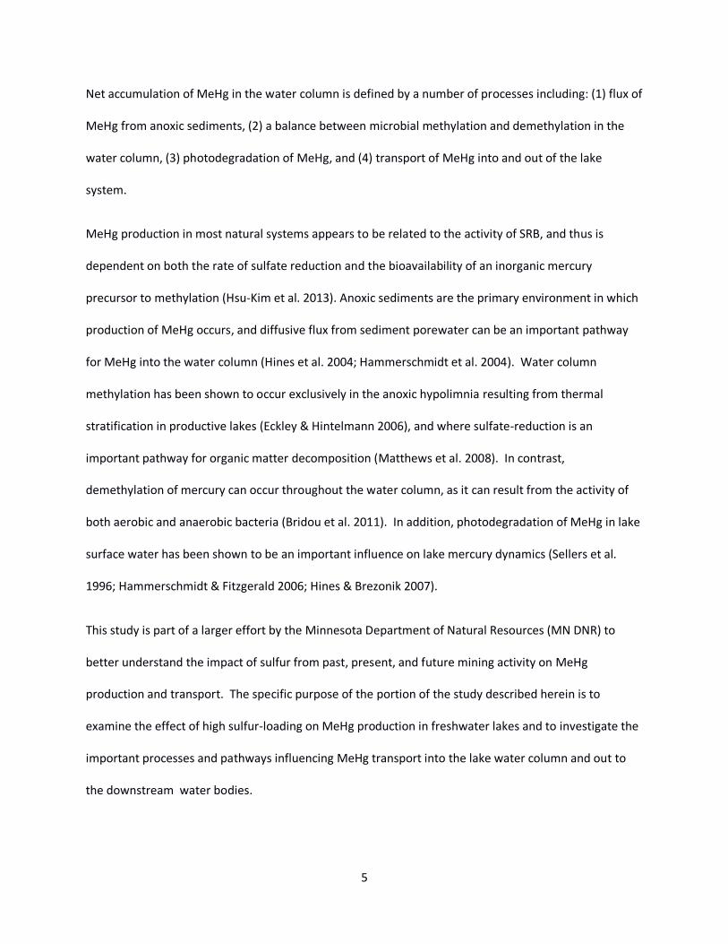
Net accumulation of MeHg in the water column is defined by a number of processes including: (1) flux of

MeHg from anoxic sediments, (2) a balance between microbial methylation and demethylation in the

water column, (3) photodegradation of MeHg, and (4) transport of MeHg into and out of the lake

system.

MeHg production in most natural systems appears to be related to the activity of SRB, and thus is

dependent on both the rate of sulfate reduction and the bioavailability of an inorganic mercury

precursor to methylation (Hsu-Kim et al. 2013). Anoxic sediments are the primary environment in which

production of MeHg occurs, and diffusive flux from sediment porewater can be an important pathway

for MeHg into the water column (Hines et al. 2004; Hammerschmidt et al. 2004). Water column

methylation has been shown to occur exclusively in the anoxic hypolimnia resulting from thermal

stratification in productive lakes (Eckley & Hintelmann 2006), and where sulfate-reduction is an

important pathway for organic matter decomposition (Matthews et al. 2008). In contrast,

demethylation of mercury can occur throughout the water column, as it can result from the activity of

both aerobic and anaerobic bacteria (Bridou et al. 2011). In addition, photodegradation of MeHg in lake

surface water has been shown to be an important influence on lake mercury dynamics (Sellers et al.

1996; Hammerschmidt & Fitzgerald 2006; Hines & Brezonik 2007).

This study is part of a larger effort by the Minnesota Department of Natural Resources (MN DNR) to

better understand the impact of sulfur from past, present, and future mining activity on MeHg

production and transport. The specific purpose of the portion of the study described herein is to

examine the effect of high sulfur-loading on MeHg production in freshwater lakes and to investigate the

important processes and pathways influencing MeHg transport into the lake water column and out to

the downstream water bodies.

6

Methods

Site Description

The two lakes investigated in this study are located in the upper reaches of the St. Louis River watershed

in northeastern Minnesota, USA, an area influenced by historic and ongoing taconite-ore mining activity

(Fig 1). Lake Manganika (N 47.49◦, W 92.57◦) is a hypereutrophic lake of maximum depth ~24 feet and

surface area ~0.67 km2, subjected to high sulfur and organic carbon loading from two inlets: dewatering

activities from a taconite pit, and discharge from an approximately 4.2 MGD (175 L/s) local municipal

wastewater plant (Berndt & Bavin 2011). Surface water sulfate concentrations range from 200-600

mg/L and excessive algal growth has historically been observed. Strong thermal stratification at 8-10

feet below the water surface was observed in Manganika from spring until mid-fall 2012 (Fig 2) although

observations in summer 2004 suggest minimal thermal stratification (Berndt and Bavin 2011).

Lake McQuade (N 47.42◦, W 92.77◦) is a mesotrophic lake with maximum depth ~20 feet and surface

area ~0.68 km2, with comparably lower surface water sulfate concentrations (30-120 mg/L in 2012).

However, consistent with increases in inlet river sulfate, observations of surface water sulfate were

approximately 300 mg/L during spring 2013. Surface water observations at two locations were very

similar, but lateral mixing of the lake may be incomplete at times due to the close proximity of the inlet

and outlet streams on the northeastern edge of the lake and a narrow pinch point in the southern half

of the lake. The deeper southern portion of Lake McQuade stratified in early summer 2012 (limnetic

surface between 8-10 feet), with a hypolimnion persisting through mid-September.

7

Fig. 1.(a) Location of the St. Louis River Watershed in Minnesota, USA. Black rectangle corresponds to location of inset (b) Location of lakes in the Mesabi Iron Range. Black line represents the northern boundary of the St. Louis River watershed; shaded regions represent mining influenced landscapes.

(a)

(b)

8

Fig. 2. Map of Lake McQuade (left) and Lake Manganika (right) sampling locations, with labeled inlet and outlet streams and bathymetry contours.

Sampling design

Water samples were collected from two locations within the lakes: a deeper basin location (depth of 15-

18 feet in McQuade; 20-25 feet in Manganika) and a shallower basin location (8-10 feet in both lakes)

and analyzed for total- and methyl- mercury as well as a host of geochemical parameters. The shallower

locations corresponded with depths very near the limnetic surface through most of the summer. The

deep sampling locations were labeled as 'Mng 1' and 'McQ 3’; the shallower sampling locations were

labeled as 'Mng 2' and 'McQ 2'. Surface water and bottom water samples, in addition to depth profiles

of general chemistry (hydrolab), were collected every 2-3 weeks from May to October 2012, and once in

June 2013, totaling ten sampling trips.

A more intensive water column sampling scheme was employed at the deep sampling locations in June,

July, August, and October 2012. Grab samples were collected at 4-6 depths spaced 2-5 feet apart in

9

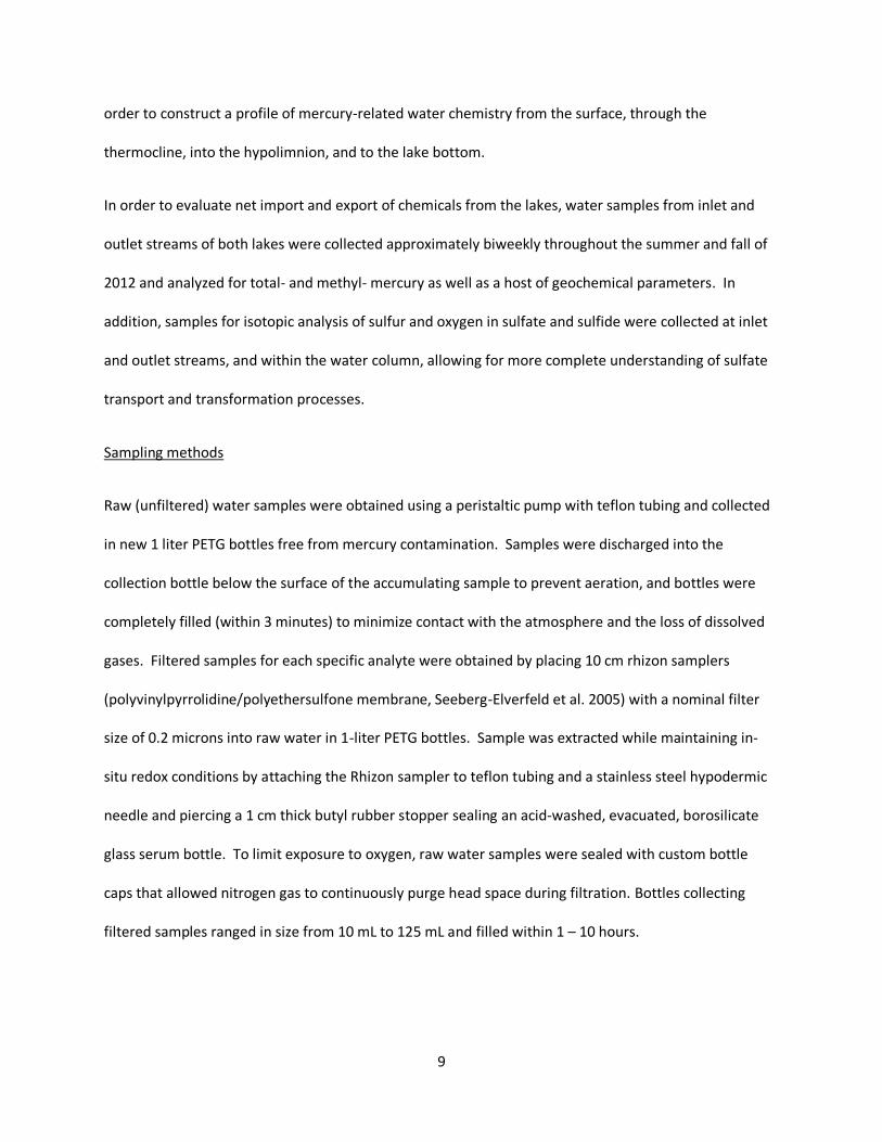
order to construct a profile of mercury-related water chemistry from the surface, through the

thermocline, into the hypolimnion, and to the lake bottom.

In order to evaluate net import and export of chemicals from the lakes, water samples from inlet and

outlet streams of both lakes were collected approximately biweekly throughout the summer and fall of

2012 and analyzed for total- and methyl- mercury as well as a host of geochemical parameters. In

addition, samples for isotopic analysis of sulfur and oxygen in sulfate and sulfide were collected at inlet

and outlet streams, and within the water column, allowing for more complete understanding of sulfate

transport and transformation processes.

Sampling methods

Raw (unfiltered) water samples were obtained using a peristaltic pump with teflon tubing and collected

in new 1 liter PETG bottles free from mercury contamination. Samples were discharged into the

collection bottle below the surface of the accumulating sample to prevent aeration, and bottles were

completely filled (within 3 minutes) to minimize contact with the atmosphere and the loss of dissolved

gases. Filtered samples for each specific analyte were obtained by placing 10 cm rhizon samplers

(polyvinylpyrrolidine/polyethersulfone membrane, Seeberg-Elverfeld et al. 2005) with a nominal filter

size of 0.2 microns into raw water in 1-liter PETG bottles. Sample was extracted while maintaining in-

situ redox conditions by attaching the Rhizon sampler to teflon tubing and a stainless steel hypodermic

needle and piercing a 1 cm thick butyl rubber stopper sealing an acid-washed, evacuated, borosilicate

glass serum bottle. To limit exposure to oxygen, raw water samples were sealed with custom bottle

caps that allowed nitrogen gas to continuously purge head space during filtration. Bottles collecting

filtered samples ranged in size from 10 mL to 125 mL and filled within 1 – 10 hours.

10

Water Column Methylation and Demethylation Rate Potentials & Mercury Analyses

The potential for Hg methylation and MeHg demethylation were assessed via enriched stable isotope

incubation techniques (Eckley & Hintelmann 2006; Mitchell & Gilmour 2008). Potential methylation and

demethylation rate constants were measured by injecting raw unfiltered water samples with a mixture

of stable isotope-enriched 200Hg2+ & Me201Hg+ (94.3% 200Hg2+ and 84.7% Me201Hg+) pre-equilibrated with

filtered site water, incubating the samples in the dark at in-situ temperatures for approximately 24

hours, freezing to finish the assays, and then measuring the generation of enriched Me200Hg+ and loss of

enriched Me201Hg+ via ICP-MS detection. Incubations took place in a mercury-free, 250 mL PETG bottle

fitted with a 1 cm thick butyl rubber stopper through which isotopes were injected using a 100 l

gastight syringe.

For THg analysis (including detection of enriched isotopes), ~0.5% by volume of BrCl was added to the

water samples to oxidize all Hg in the sample to Hg(II). After allowing to react overnight, THg was

characterized following the USEPA method 1631 using a Tekran 2600 automated Hg analysis system that

was hyphenated with an Agilent 7700x ICP-MS for detection of individual Hg isotopes. For MeHg

analysis, water samples were distilled according to the methods of Horvat et al. (1993), but with the

addition of a different enriched MeHg spike (Me199Hg), for MeHg determination by isotope-dilution

techniques (Hintelmann and Evans, 1997). All analyses used calculations from Hintelmann and Ogrinc

(2003) to account for the <100% enrichment of isotopes in calculating enriched 200Hg and 201Hg

concentration in THg and MeHg, as well as in calculating ambient THg and MeHg levels from the

dominant naturally occurring 202Hg isotope.

The methylation (kmeth) and demethylation (kdemeth) rate constants were calculated by:

[ ] [ ]⁄

11

([ ] [ ]) [ ]⁄

[ ]

Clean hands protocols were utilized for mercury samples throughout sample handling, preservation, and

analysis, and water samples were preserved by adding concentrated trace metal HCl to a concentration

of 0.5%. Filtered water samples were analyzed for MeHg by isotope-dilution ICP-MS following

distillation, as explained above (Hintelmann and Evans, 1997; Horvat et al., 1993), and THg according to

USEPA method 1631, using a Tekran 2600 automated mercury analyzer. Inorganic mercury (iHg)

concentrations were calculated by subtracting the MeHg concentration from the THg concentration, i.e.

mercury was assumed to exist as either MeHg or iHg.

Chemical Analysis

A Hydrolab S5 sonde was used to take biweekly in-situ depth profiles with 3 foot depth increments at

each sampling location. The sonde contained probes to measure for temperature, pH, dissolved oxygen

(LDO), conductivity, and redox potential (ORP) and was calibrated immediately prior to use.

Filtered water samples for anion analysis were acidified to a pH<3 with HCl and bubbled with N2 gas for

15 minutes to remove dissolved sulfide. A non-acidified duplicate sample was split from selected

samples for chloride analysis. Sulfate (SO42-), nitrate (NO3

-), phosphate (PO43-), and chloride (Cl-) were

quantified via ion chromatography (Method 300.1, USEPA 1997) on a Dionex ICS 1100 system. Water

samples for dissolved sulfide (H2S + HS-) analysis were filtered into an evacuated serum bottle preloaded

with ZnAc and NaOH preservative and quantified using automated methylene blue method (4500-S2- E,

Eaton 2005). Dissolved ferrous iron (Fe2+) was quantified photometrically using the Phenanthroline

Method (3500-FeB) (Eaton 2005). Ammonium was analyzed colorimetrically at the St. Croix Watershed

Research Station (SCWRS) laboratory using the phenolate method (Lachat QuikChem method 10-107-

12

06-1-B). Dissolved organic carbon (DOC) and dissolved inorganic carbon (DIC) were quantified on a

Teledyne-Tekmar Torch Combustion TOC Analyzer. Dissolved carbon lability was assessed by analyzing

samples for specific ultraviolet absorption at 254nm (SUVA, Weishaar et al. 2003) and spectral slope

ratio (Helms et al. 2008) on a Varian Cary 50 scanning UV-Vis spectrophotometer to provide an

indication of aromaticity and relative molecular weight, respectively.

Flux Equation

Estimates of methyl- and inorganic- mercury diffusive flux from lake sediment utilized filtered bottom

water samples as well as filtered lake sediment porewater samples reported in earlier sections of this

report (Bailey et al. 2013). Flux was estimated following a method employed by similar studies (Gill et

al. 1999; Hammerschmidt et al. 2004), using an equation derived from Fick’s first law and assuming no

bulk water movement:

(

)

where diffusive flux (J) is a function of the change in concentration across the sediment-water interface

(SWI), sediment porosity (ϕ), tortuosity (θ2), and the diffusion coefficient of the chemical in water(Dw).

Water-only diffusion was corrected for measured bottom water temperature (Li & Gregory 1974;

Boudreau 1997). The concentration derivative was calculated using difference between filtered bottom

water concentration and filtered porewater concentration of the composited 0-2 cm sediment sample,

assuming 1 cm represented the change in depth between the concentrations. Sediment porosity was

calculated using measured dry bulk density (b) and particle density (s):

( )

with s estimated using measured fractions of sediment composition:

13

Tortuosity was calculated using sediment porosity, based on the relationship for unlithified fine-grained

sediments proposed by Boudreau 1996.

( )

MeHg diffusion coefficient was estimated using the relationship with molar volume (Vm) for neutrally

charged aqueous species (Hayduk & Laudie 1974; Schwarzenbach et al. 1993; Hammerschmidt et al.

2004):

(

)

with the molar volume calculated from molecular weight and the density of the species (ATSDR 1999).

For the purpose of estimating diffusion coefficients, MeHg was assumed to be present in the form

CH3HgSH0 (Dyrssen & Wedborg 1991; Hammerschmidt et al. 2004)a form of mercury hypothesized to be

present in Lake Manganika and other sulfide rich waters of the region by Berndt & Bavin (2011). The

diffusion coefficient of inorganic mercury was assumed to be 5.5 X 10-6 cm-2 s-1 based on values used in

previous studies (Bothner et al. 1980; Gobeil & Costa 1993; Covelli et al. 1999).

Results & Discussion

A. Investigation of Hg Analyses

Inter-lab Comparison

Water samples of inlet and outlet streams were filtered using a nominal filter size of 0.45 microns and

were analyzed for Hg at the Gustavus Adolphus College laboratory, while water column samples were

filtered through a 0.2 micron filter and were analyzed at the University of Toronto laboratory. To

compare Hg analysis between the two labs, concurrent water column samples were collected and

14

filtered using both filter sizes and analyzed at the two labs (Table A). Measured concentrations between

the two labs were correlated for both THg (R2 = 0.66) and MeHg (R2 = 0.66) (Fig 3a, 3c). This correlation

was also present for THg and MeHg when analyzing the data in of each lake individually (Fig 3b, 3d).

Comparisons of the data show that as a general trend, MeHg concentrations were generally 30 to 80 %

higher in the measurements made by the Gustavus Adolphus lab, which was expected due to the use of

a larger filter size. There were, however, several exceptions to this in which MeHg quantified at

Gustavus Adolphus were 4 to 8 times larger than those quantified at Toronto. Additionally, in

Manganika surface waters, Gustavus consistently quantified concentrations lower than Toronto (Table

A). The reasons for these discrepancies are still being investigated at the time of this report. Total

mercury comparisons were less variable between labs with values quantified at Gustavus typically falling

between 50 and 150 % of those at Toronto, the surface waters of Lake Manganika again being an

exception (Table A).

Filtered v. Unfiltered MeHg Samples

Dissolved MeHg and THg concentrations quantified most commonly in this study do not account for the

total mass in the water column, because filtered samples were used to quantify MeHg and THg. In an

effort to account for the entire Hg pool, several raw (unfiltered) water samples were quantified for

MeHg and THg in addition to the filtered samples by the Gustavus Adolphus lab to determine the

dissolved fraction of the THg and MeHg present in the water column (Table B). Due to the significant

particle concentrations in the hypereutrophic surface waters of Lake Manganika, the pool of mercury in

the unfiltered fraction represents the majority (56 – 88 %) of the total mercury pool at this location

(Table B). Waters of the mesotrophic Lake McQuade contained on average 10 to 20 % of the total

mercury pool and on the particulate (unfiltered minus filtered) phase. The particulate phase

consistently comprised 24 to 65 % of the MeHg in the surface waters, but only 19 % of MeHg on average

15

in the bottom waters. These comparisons were used to help analyze and better understand mercury

dynamics and export, as described in later sections.

B. Lake Manganika

Thermal stratification and anoxic conditions were observed in the deepest site at Lake Manganika from

the onset of sampling in May 2012 until complete lake mixing occurred in mid-September (Fig 4a, 4b).

The thermocline and redoxcline, consistently present between 7-13 feet, were strongest in July (Fig 7b)

and, though temperature and pH profiles suggest the lake began to mix at intermediate depths in mid-

August (Fig 7c, Fig 4c), reducing conditions persisted in the bottom waters through early to mid-

September (Fig 4a,d). At the shallower site, Mng 2 (approximate depth: 9ft), the sediment surface

remained below the thermocline until mid-August (Fig 5b), with anoxic conditions measured from early

July to the end of August (Fig 5a).

Several geochemical observations provided evidence of active sulfate reduction in the bottom waters of

the deepest portions of Lake Manganika. Sulfate concentrations decreased in Mng1 bottom waters

between mid-June and early-August (Fig 4c, 7b) while depth profiles showed that sulfate concentrations

remained homogenous in the epilimnion (Fig 7a & 7b). During this time, bottom waters experienced an

increase in sulfide concentration, as well as thiosulfate (Fig 4e), a sulfur oxyanion which can

disproportionate to sulfate and sulfide. The decrease in bottom water sulfate while surface water

sulfate was rising (Fib 4c) suggests rapid consumption of sulfate in the hydrologically isolated

hypolimnion. The speed of sulfate consumption (~50 mol/L/day during July, Fig 4c), coupled with

increases in reduced sulfur species in bottom waters and very low ORP measurements (Appendix B),

suggest that active sulfate reduction was occurring above the sediment-water interface in the bottom

waters of Lake Manganika.

16

Isotope data from Mng1 bottom water samples provides additional evidence for bottom water sulfate

reduction. Because sulfate reduction preferentially targets molecules with lighter isotopes, the isotope

fractionation of the remaining sulfate pool will be increasingly more positive (heavier) as sulfate

reduction progresses. 34SSO4 in bottom waters was elevated (heavier) relative to sulfate in surface

waters and 34SHS in bottom waters was lower (lighter) relative to sulfate in surface waters (Fig 16). This

observation provides strong evidence for active hypolimnetic reduction of sulfate supplied from surface

waters. Consistent with the presence of thiosulfate in bottom waters, the trajectory of the 18OSO4 to

34SSO4 ratio in Lake Manganika’s bottom waters further suggests that the sulfate reduction pathway is

different from that observed in many other parts of the watershed (Kelly & Berndt 2013).

An increase in dissolved MeHg concentration to >3 ng/L occurred in the bottom waters of Mng1 in

August (Fig 4g). The similar timing between the increase in MeHg and evidence of sulfate reduction in

the hypolimnion, along with a corresponding increase in %MeHg (Fig 4f), resulting from relatively

constant concentrations of inorganic mercury in bottom waters (Fig 4h), suggests bottom water

methylation at Mng1 likely contributed to the increase in MeHg. The elevated BW dissolved MeHg

observation in mid-May (>95 % MeHg, Fig 4f, g) could be a result of net methyl mercury production in

the absence of high sulfide concentrations early in the year. This is supported by the measurement of

methylation rates in Mng1 bottom water samples collected during late spring conditions (June 2013,

Table C). However, it is also consistent with elevated MeHg observed in lake sediment pore fluids during

spring and early summer, interpreted to be a result of lower biological activity and a greater influence of

solid-liquid partitioning (Bailey et al. 2013). Though only a portion of the total- and methyl- mercury

pool was present in the dissolved phase, the increases in hypolimnetic dissolved MeHg observed in a

location supporting active sulfate reduction points towards in-situ production rather than changes due

to partitioning from the solid phase.

17

In contrast to the deepest portion of the lake, MeHg concentrations in the bottom waters of Mng2 were

uniformly below 0.2 ng/L throughout the year with %MeHg consistently lower than those at Mng1 (Fig

5f & 5g). This was likely due to nitrate, which was present in Mng 2 bottom waters (near the

thermocline) in July (Fig 5d), but was absent below the thermocline (Fig 7b) and in the deep hypolimnion

until early September (Fig 4d). Because nitrate is more energetically favorable than sulfate, sulfate

reduction occurs only in environments where nitrate has been depleted (Matthews et al. 2008), thus the

presence of nitrate will have an inhibitory effect on net methylation (Todorova et al. 2008). This effect is

illustrated by the absence of methylation at the limnetic surface of Manganika (12.5 ft in June 2013,

Table C), which had nitrate concentrations almost twice as high as in the bottom water, where

methylation was quantified (Table C). The absence of sulfide at the bottom waters of Mng 2 (~9 ft water

depth) throughout the summer (Fig 5e), further suggests that sulfate reduction was confined to the

sediment in portions of the lake shallower than the thermocline (8-12 feet) and likely only extended into

bottom waters in the deepest portion of the lake (Fig 3).

Dissolved MeHg and iHg were generally lower in the epilimnion relative to the hypolimnion throughout

the year until lake turnover, with iHg concentrations ranging from 0.5 – 2 ng/L and MeHg concentrations

< 1 ng/L in the surface water (Fig 4g-h, Fig 7a-c). However, the observed decrease in dissolved MeHg

concentrations between the hypolimnion and epilimnion may not reflect the entire mercury pool. In the

bottom waters of Lake Manganika, 24.0 % of the THg present was in the dissolved phase on average,

with a similar dissolved fraction of THg seen in the surface waters (18.6 % average) (Table B). In

contrast, the fraction of MeHg in the dissolved phase was very different between surface and bottom

waters, representing a majority of the MeHg present in the bottom water (78.3 % average) but only a

small fraction in the surface water (6.5 % average). Though several comparisons between filtered and

unfiltered total- and methyl - mercury were made (Table B), at the time of this report an attempt has

not been made to use an adjustment factor to quantitatively compare the total mercury pools in the

18

waters sampled. The results of additional data analysis and coordination with data sets from other

groups may warrant a quantitative comparison in the future. High levels of algae and other organic

matter in the surface waters of hypereutrophic lakes adsorb and otherwise incorporate much of the

dissolved MeHg to particles larger than the nominal filter size, causing a large fraction of the MeHg

present in the surface water to be excluded from the dissolved concentration (Pickhardt et al. 2002).

The increase in surface water % MeHg (dissolved) in mid-summer could have been due to interactions

with the solid phase or reduced photodemethylation as algal densities increased.

C. Lake McQuade

Lake McQuade thermally stratified in the early summer of 2012 (Fig 9b & 11), with low dissolved oxygen

concentrations persisting in the hypolimnion until mid-September (Fig 9a). The limnetic surface was

shllow enough to create anoxic conditions above the sediment surface of McQ2 (depth = 9 ft) until mid-

August (Fig 10a).

Hypolimnetic sulfate concentrations at McQ3 declined by a total of ~0.3 mmol/L between late-June and

mid-August during a time when sulfate was steadily increasing in the surface waters (Fig 9c). This

suggests consumption of sulfate in the hydrologically isolated hypolimnion (Fig 9j), though sulfide

concentrations in the hypolimnion remained relatively low throughout the year (<0.02 mmol/L) (Fig 9e

& 10e). The presence of aqueous ferrous iron at 0.01 - 0.025 mmol/L in hypolimnetic waters during July

and August (Fig 9i) suggests that sulfide-iron(II) precipitation reactions limited the dissolved sulfide able

to accumulate in the bottom waters. Dissolved phosphorus in bottom waters averaged greater than

0.015 mM, suggesting release from dissolving iron oxide phases in sediments.

Bottom water sulfate increased sharply in mid-August (Fig 9a) due to mixing with the epilimnion (Fig

11d, Fig 9j), but anoxic conditions in bottom waters re-established quickly (Fig 12c). Hypolimnion sulfate

again diverged from surface water sulfate from late August to early September (Fig 9c), suggesting that

19

sulfate consumption continued in the bottom waters following lake turnover. This observation is

consistent with findings by Phelps & Zeikus 1985, which demonstrated active sulfate reduction in

bottom waters and sediment porewaters directly following lake turnover. Though the surface waters

also contained significant sulfate, the mixing of oxic surface waters with reduced bottom waters has

been shown to result in the re-oxidation of reduced species in bottom waters and sediments. This can,

in turn, supply favorable electron acceptors (oxidized iron and sulfate) for microbial metabolism if

anoxic conditions are re-established in the bottom waters and/or sediment porewaters. Bottom water

ammonia concentrations averaged nearly 0.1 mM in July and August and may explain the observed

increase in bottom water nitrate following turnover (Fig 9d), as well as the increase of sulfate in

McQuade sediment porewaters from July to October (Bailey et al. 2013).

Isotope analysis of sulfate molecules in the inlet and outlet of McQuade showed that both 18OSO4 and

34SSO4 were increased in outlet samples compared to the inlet (Upstream McQuade and Downstream

McQuade, Fig 17), indicating that sulfate reduction occurred within the lake. Isotope analysis of bottom

water samples also suggested sulfate reduction in the bottom waters, particularly in late August and

early September following lake turnover (McQuade surface and McQuade bottom, Figure 17; Kelly &

Berndt 2013). The observed shifts in δ34SO4 in bottom water sulfate further supports the hypothesis

that sulfate reduction occurred in McQuade bottom waters both before and after lake turnover.

Bottom water MeHg concentrations at the deep site of Lake McQuade ranged between 1.0 – 2.5 ng/L

for most of the summer, with the exception of a much higher concentration in early August (Fig 9g).

This rise of up to more than 6 ng/L MeHg was also reflected in %MeHg (Fig 9f), and occurred while

inorganic mercury concentrations were consistently between 1-2 ng/L (Fig 9i). Similar to Lake

Manganika, elevated MeHg concentration and %MeHg occurred in bottom waters during late-July and

early-August and corresponded with a period of decreasing sulfate in bottom waters. This time period

20

also coincided with a rise in bottom water DOC concentrations (Fig 9k). Fresh DOC supplied during a

time when conditions were favorable for sulfate reduction may have facilitated more rapid sulfate

reduction or increased the concentration or bioavailability of inorganic mercury, driving the production

of MeHg at a faster rate. Additionally, since sulfide was present at low concentrations, DOC may have

acted as the primary ligand for MeHg; thus, it is possible that the concentration of DOC influenced the

capacity for bottom waters to hold dissolved MeHg.

Depth profiles at the deepest portion of McQuade Lake revealed higher %MeHg (25-50%) at depths

below the redoxcline than at oxygenated shallower depths where no sulfate was being consumed (<

25%) (Fig 12a-c). This behavior was consistent in all three summer depth profiles, suggesting a

connection with sulfate reduction in the hypolimnion. This implies that even though dissolved sulfide

concentrations were near detection limits, sulfate reduction has an influence of mercury dynamics in

the bottom waters – an influence that may be enhanced by increased DOC concentrations. Methylation

rates were not detected in McQuade bottom water samples collected in June 2013 (Table C), though

because the late spring season does not capture lake conditions favorable to sulfate reduction, it is

expected that water column methylation will be negligible at that time.

D. Estimated sediment flux of Methyl- and inorganic- mercury

MeHg concentrations in the anoxic hypolimnion are a result of net methylation or demethylation as well

as diffusive flux across the sediment-water interface. As the biogeochemical conditions influencing

mercury dynamics can vary greatly between porewater and bottom water, diffusive flux can vary

substantially over the course of the year. A caveat to these estimates is that diffusive flux may not be

solely responsible for transport at the SWI. This is particularly relevant to Lake Manganika, where

evidence of bubbles in the hypolimnon were observed during sample collection (Engstrom, Johnson,

personal communication) and ebullition of methane has been previously hypothesized (Berndt & Bavin

21

2011). Additionally, methane was quantified in bottom waters of both lakes during summer 2012

(Berndt and Kelley, unpublished data).

Estimates of diffusive MeHg flux at Mng1 ranged from -18.0 to 70.8 pmol/m2/d, with negative fluxes (i.e.

into the sediment) estimated for the May and July 2012 data, while MeHg flux at Mng2 was always

positive (i.e. towards the water column) and ranged from 1.3 to 186.8 pmol/m2/d (Table D). Estimates

of diffusive MeHg flux at Mng1 were highest in October 2012, possibly due to decreased bottom water

MeHg concentrations resulting from lake mixing. A possible explanation for the negative flux values in

May and July could be methylation in the bottom waters causing a build-up of MeHg in the spring and

early summer, while MeHg concentrations stayed low in the sediment porewater due to high sulfide

concentrations inhibiting production.

Diffusive flux estimates of inorganic mercury at Mng1 (range: -5.2 to 391.4 pmol/m2/d) were also

negative in July 2012 but positive at all other times, while inorganic mercury flux at Mng2 (range: -9.0 to

26.9 pmol/m2/d) was positive in July 2012, but negative in October 2012 and June 2013 (Table D). It

should be noted that fluxes of inorganic mercury were estimated assuming aqueous inorganic mercury

existed as neutral complexes, while proposed mercury speciation models suggest that charged species

dominate at sulfide concentrations equivalent to those present in Manganika sediment (Benoit et al.

1999). If this is the case, the inorganic mercury diffusion coefficient used to calculate flux estimates

would then be overestimating the diffusive ability of the inorganic mercury species.

Diffusive flux of MeHg from Lake McQuade sediment was positive throughout the summer and ranged

from 8.5 – 38.3 pmol/m2/d at McQ3 and 5.0 – 11.6 pmol/m2/d at McQ2 (Table D). Diffusive MeHg flux

estimates at both sampling locations at Lake McQuade displayed similar seasonal trends, with the

lowest flux occurring in July 2012, the median in October 2012, and the highest in June 2013 (Fig 15).

During the late spring conditions in June 2013 MeHg production was likely occurring in the sediment but

22

because the lake had not yet stratified, methylation was not measured in the bottom waters (Table C).

Conditions after lake stratification promote MeHg production, resulting in an increase in %MeHg and

MeHg concentrations in the bottom waters and lower flux values in the summer months.

E. Net Export

Lake Manganika

Dissolved MeHg concentrations in the outlet from Lake Manganika remained uniformly low (<0.1 ng/L)

throughout the year, despite (1) high MeHg concentrations in the bottom water (peaking at 3.3 ng/L),

(2) evidence of MeHg production in the bottom waters under anoxic conditions, and (3) MeHg

concentrations of 0.9 – 2.9 ng/L in the inlet from the municipal wastewater treatment plant. This may

be due to net demethylation in the epilimnion resulting from demethylating aerobic bacteria and/or

photo-degradation, or due to limited mixing between the epilimnion and the hypolimnion physically

trapping the MeHg in the bottom waters. It is more likely, however, that due to the high levels of algal

particles in the surface waters of Manganika much of the MeHg transported out of the epilimnion was

adsorbed to particles too large to pass into the filtered samples, and thus were not accounted for in the

outlet data. MeHg concentrations in unfiltered outlet water samples were around 10 times higher than

MeHg concentrations in the filtered samples (TableB). This large portion of the total mercury pool

(unfiltered fraction) was not consistently quantified and therefore presents a serious challenge for

detailed accounting of MeHg in Lake Manganika.

Lake McQuade

Bottom water concentrations of MeHg were consistently elevated above surface water concentrations

at McQ3, suggesting a spatial gradient to drive net transport of MeHg from bottom to surface waters

(Fig 9g). However, the close similarity between inlet, surface, and outlet concentrations of total- and

23

methyl- mercury in May and June 2012 implies that the MeHg produced in the anoxic bottom water and

sediment of Lake McQuade was contained in the hypolimnion, and therefore not transported out of the

lake (Fig 13a). The capacity for transport out of the hypolimnion is limited by the mixing rate at the

limnetic surface, which can be estimated with temperature profile data using the Flux-gradient method

(Jassby & Powell 1975). The vertical diffusion coefficient calculated at the limnetic surface (11-12 ft) in

early August was -1.33 X 10-3 cm2/s, on the low end of values reported for other small inland water

bodies (0.005 – 0.09 cm2/s, Lake Onondaga; Matthews & Effler 2006)

Conductivity, magnesium, and sulfate steadily increased in the surface waters of Lake McQuade over the

course of the summer (Fig 9c, 9j, 9l, 10c, 10j) in response to a rather abrupt increase in inlet

concentrations in early July (Fig 13d, 13e, 13h). A simple mixing model based on observations of

magnesium at the inlet and outlet of Lake McQuade in response to the relative step increase in early

July was used to estimate an average hydraulic residence time of between 45 and 60 days (Appendix A).

The lower sulfate observed in the outlet at the end of the summer, even when outlet magnesium was

similar to inlet magnesium, can be described by an effective first order, areal mass transport coefficient

of 0.0087 m/day. Appendix A provides an outline of preliminary calculations, including an estimate for

the net methylmercury flux from hypolimnon to epilimnon and demethylation rate in the epilimnion.

These calculations are preliminary at the time of this report and will be refined with input from other

project partners.

Basic mixing calculations were performed to investigate if enough MeHg mass was present in

hypolimnion waters to explain the observed increase in the outlet concentrations following lake

turnover (Fig 13a). In lake samples taken on 8/21/2012 (immediately prior to the MeHg increase

observed in the outlet) MeHg concentrations in surface and bottom waters were 0.08 and 1.99 ng/L

respectively (Table E). Assuming conservative mixing (i.e. ignoring inputs, methylation and

24

demethylation reactions), complete mixing of the lake epilimnion and hypolimnion on 8/21/2012 would

result in a MeHg concentration of 0.23 ng/L in the mixed, which equates to a 0.15 ng/L increase from

the original surface water concentration on 8/21/2012.

Outlet MeHg concentrations were 0.15 – 0.2 in early August and rose to 0.35 ng/L on 8/27, suggesting

that much of this increase can be explained by increased surface water MeHg related to lake mixing. In

light of the estimated 1 to 2 month residence time of the lake (Appendix A) a rapid increase in outlet

MeHg seems unlikely without an sudden change in a process or condition internal to the lake. The

coincidence of an increase in outlet MeHg with evidence of lake turnover further supports the

hypothesis that summer thermal stratification acts to contain most MeHg in the hypolimnion. Net

export of MeHg from McQuade (outlet minus inlet concentration) was largest in the weeks following

lake turnover when the stable limnetic surface was removed. Net export then decreased later in the

fall, likely due to net demethylation in the aerobic water column.

At Lake McQuade, outlet DOC concentrations were consistently higher than inlet DOC throughout the

year implying that Lake McQuade is a net source of DOC to the downstream system (Fig 14a). MeHg

concentrations were positively correlated with DOC concentrations in both the inlet and outlet streams,

and linear trendlines of the inlet and outlet have similar slopes with the outlet trendline shifted to the

right (higher DOC concentrations) (Fig 14b). This means that for equivalent DOC concentrations, outlet

MeHg concentrations are lower than inlet concentrations. A previous study of DOC and MeHg in the

same watershed proposed that DOC pools composed of heavier molecules had a reduced capacity to

carry MeHg (Berndt & Bavin 2012). Thus one explanation for the shift in the MeHg:DOC slope is that the

DOC added in Lake McQuade was of higher molecular weight, causing the shift in MeHg binding capacity

(Berndt & Bavin 2012).

25

Conclusions

Though significant differences exist among the two lakes presented here, both geochemical and isotopic

evidence point towards significant sulfate reduction in the hypolimnion of Lake Manganika and Lake

McQuade. Evidence suggests that water column methylation associated with the observed sulfate

reduction has an impact on dissolved MeHg concentrations mostly in the hypolimnion. Flux of MeHg

from sediment may also be impacting bottom water MeHg concentrations. A driving force for diffusive

flux from porewaters to bottom waters existed for most of the summer at Lake McQuade, while

resuspension of sediment-associated MeHg due to ebullition of methane bubbles could be a a source of

MeHg at Lake Manganika. Quantitative accounting of MeHg is difficult at Lake Manganika due to a

significant particle-associated component not quantified in filtered samples.

Despite production of MeHg in bottom waters and sediment porewaters, there is little evidence of

MeHg export out of the lakes into the downstream water systems while lakes are stably stratified, likely

due to limited exchange across the limnetic surface. At McQuade, export of MeHg appears to be

highest during a brief period from after lake turnover, when mixing brought MeHg from the hypolimnion

to the surface, until net demethylation has diminished MeHg concentrations in the water column. This

process likely applies to both lakes, though quantitative accounting is difficult at Lake Manganika due to

the export of MeHg bound to filterable particulate matter. Future mass balance modeling and

quantitative data analysis will lead to a more robust and nuanced understanding of MeHg transport

within and out of the lakes.

26

Upcoming Work

The preliminary interpretations included in this report will be shared with other project partners and

refined in light of relevant observations and analysis. Future work is likely to include a mercury mass

balance on the hypolimnion of both lakes to help quantify the relative influence of sediment flux, water

column methylation and demethylation, and flux across the limnetic surface. This will require the

calculation of the rate of vertical diffusion across the limnetic surface for each biweekly temperature

profile at each sampling site, using the Flux-gradient method (Jassby & Powell 1975). Estimates will be

made for typical conditions from spring to fall, using measured concentrations of redox species and flux

estimates as boundary conditions. By quantifying different aspects of the mercury dynamics in the

lakes, we will better understand the primary pathways for MeHg production and transport in these

lakes.

In addition, refined estimates for lake residence time will be made at McQuade by further examining

inlet, surface water, and outlet concentrations of conservative species, such as Magnesium (Mg).

Calculation of a residence time will help to further understanding of the mass balance of sulfate and

MeHg and the importance and magnitude of net export to the downstream water systems. A

preliminary lake mixing model is included as Appendix A and will be expanded to more fully consider

interactions with the hypolimnion and implications for transport across the limnetic surface.

27

References

Bailey, L. T., Johnson, N. W., Mitchell, C. P., Engstrom, D. R., Berndt, M. E., Coleman-Wasik, J. 2013. Geochemical factors influencing methylmercury production and partitioning in sulfate-impacted lake sediments. Final Project Data Report. MN Department of Natural Resources, Division of Lands and Minerals.

Bak, F., & Cypionka, H. (1987). A novel type of energy metabolism involving fermentation of inorganic sulphur

compounds. Benoit, J. M., Gilmour, C. C., Mason, R. P., & Heyes, A. (1999). Sulfide controls on mercury speciation and

bioavailability to methylating bacteria in sediment pore waters. Environmental Science & Technology, 33(6), 951-957.

Berndt, M. E., & Bavin, T. K. (2011). Sulfate and mercury cycling in five wetlands and a lake receiving sulfate from

taconite mines in northeastern Minnesota. Minnesota Department of Natural Resources, Division of Lands and Minerals. St. Paul, MN.

Berndt, M. E., & Bavin, T. K. (2012). Methylmercury and dissolved organic carbon relationships in a wetland-rich

watershed impacted by elevated sulfate from mining. Environmental Pollution, 161, 321-327. Bloom, N. S. (1992). On the chemical form of mercury in edible fish and marine invertebrate tissue. Canadian

Journal of Fisheries and Aquatic Sciences, 49(5), 1010-1017. Bothner, M. H., Jahnke, R. A., Peterson, M. L., & Carpenter, R. (1980). Rate of mercury loss from contaminated

estuarine sediments. Geochimica et Cosmochimica Acta, 44(2), 273-285. Boudreau, B. P. (1996). The diffusive tortuosity of fine-grained unlithified sediments. Geochimica et Cosmochimica

Acta, 60(16), 3139-3142. Boudreau, B. P. (1997). Diagenetic models and their implementation (Vol. 505). Berlin: Springer. Bridou, R., Monperrus, M., Gonzalez, P. R., Guyoneaud, R., & Amouroux, D. (2011). Simultaneous determination of

mercury methylation and demethylation capacities of various sulfate‐reducing bacteria using species‐specific isotopic tracers. Environmental Toxicology and Chemistry, 30(2), 337-344.

Compeau, G. C., & Bartha, R. (1985). Sulfate-reducing bacteria: principal methylators of mercury in anoxic

estuarine sediment. Applied and environmental microbiology, 50(2), 498-502. Covelli, S., Faganeli, J., Horvat, M., & Brambati, A. (1999). Porewater distribution and benthic flux measurements of

mercury and methylmercury in the Gulf of Trieste (Northern Adriatic Sea). Estuarine, Coastal and Shelf Science, 48(4), 415-428.

Dyrssen, D., & Wedborg, M. (1991). The sulphur-mercury (II) system in natural waters. Water Air & Soil Pollution,

56(1), 507-519. Eaton, A. D. (Ed.). (2005). Standard methods for the examination of water and wastewater. none. Eckley, C. S., & Hintelmann, H. (2006). Determination of mercury methylation potentials in the water column of

lakes across Canada. Science of the Total Environment, 368(1), 111-125.

28

Fleming, E. J., Mack, E. E., Green, P. G., & Nelson, D. C. (2006). Mercury methylation from unexpected sources: molybdate-inhibited freshwater sediments and an iron-reducing bacterium. Applied and environmental microbiology, 72(1), 457-464.

Gill, G. A., & Bruland, K. W. (1990). Mercury speciation in surface freshwater systems in California and other areas.

Environmental Science & Technology, 24(9), 1392-1400. Gill, G. A., Bloom, N. S., Cappellino, S., Driscoll, C. T., Dobbs, C., McShea, L., ... & Rudd, J. W. (1999). Sediment-water

fluxes of mercury in Lavaca Bay, Texas. Environmental science & technology, 33(5), 663-669. Gilmour, C. C., Henry, E. A., & Mitchell, R. (1992). Sulfate stimulation of mercury methylation in freshwater

sediments. Environmental Science & Technology, 26(11), 22 Gobeil, C., & Cossa, D. (1993). Mercury in sediments and sediment pore water in the Laurentian Trough. Canadian

Journal of Fisheries and Aquatic Sciences, 50(8), 1794-1800. Hamelin, S., Amyot, M., Barkay, T., Wang, Y., & Planas, D. (2011). Methanogens: principal methylators of mercury

in lake periphyton. Environmental science & technology, 45(18), 7693-7700. Hammerschmidt, C. R., Fitzgerald, W. F., Lamborg, C. H., Balcom, P. H., & Visscher, P. T. (2004). Biogeochemistry of

methylmercury in sediments of Long Island Sound. Marine Chemistry, 90(1), 31-52. Hammerschmidt, C. R., & Fitzgerald, W. F. (2006). Photodecomposition of methylmercury in an arctic Alaskan

lake. Environmental science & technology,40(4), 1212-1216. Hayduk, W., & Laudie, H. (1974). Prediction of diffusion coefficients for nonelectrolytes in dilute aqueous solutions.

AIChE Journal, 20(3), 611-615. Helms, J. R., A. Stubbins, J. D. Ritchie, E. C. Minor, D. J. Kieber, and K. Mopper (2008), Absorption spectral slopes

and slope ratios as indicators of molecular weight, source, and photobleaching of chromophoric dissolved organic matter, Limnol. Oceanogr., 53, 955-969.

Hildebrand, S. G., Strand, R. H., & Huckabee, J. W. (1980). Mercury accumulation in fish and invertebrates of the

North Fork Holston River, Virginia and Tennessee. Journal of Environmental Quality, 9(3), 393-400. Hines, N. A., & Brezonik, P. L. (2007). Mercury inputs and outputs at a small lake in northern Minnesota.

Biogeochemistry, 84(3), 265-284. Hines, N. A., Brezonik, P. L., & Engstrom, D. R. (2004). Sediment and porewater profiles and fluxes of mercury and

methylmercury in a small seepage lake in northern Minnesota. Environmental science & technology, 38(24), 6610-6617.

Hintelmann, H., & Evans, R. D. (1997). Application of stable isotopes in environmental tracer studies–Measurement

of monomethylmercury (CH3Hg+) by isotope dilution ICP-MS and detection of species transformation. Fresenius' journal of analytical chemistry, 358(3), 378-385.

Hintelmann, H., & Ogrinc, N. (2003, January). Determination of stable mercury isotopes by ICP/MS and their

application in environmental studies. In ACS symposium series (Vol. 835, pp. 321-338). Washington, DC; American Chemical Society; 1999.

Horvat, M., Liang, L., & Bloom, N. S. (1993). Comparison of distillation with other current isolation methods for the

determination of methyl mercury compounds in low level environmental samples: Part II. Water. Analytica Chimica Acta, 282(1), 153-168.

29

Hsu-Kim, H., Kucharzyk, K. H., Zhang, T., & Deshusses, M. A. (2013). Mechanisms regulating mercury bioavailability

for methylating microorganisms in the aquatic environment: A critical review. Environmental science &

technology, 47(6), 2441-2456. Jassby, A., & Powell, T. (1975). Vertical patterns of eddy diffusion during stratification in Castle Lake,

California. Limnology and oceanography, 530-543. Jørgensen, B. B., & Bak, F. (1991). Pathways and microbiology of thiosulfate transformations and sulfate reduction

in a marine sediment (Kattegat, Denmark). Applied and Environmental Microbiology, 57(3), 847-856. Kelly, M. J., & Berndt, M. E. (2013). An updated isotopic analysis of sulfate cycling and mixing processes in the St.

Louis River Watershed. Minnesota Department of Natural Resources, Division of Lands and Minerals. St. Paul, MN.

Kerin, E. J., Gilmour, C. C., Roden, E., Suzuki, M. T., Coates, J. D., & Mason, R. P. (2006). Mercury methylation by

dissimilatory iron-reducing bacteria.Applied and environmental microbiology, 72(12), 7919-7921. Li, Y.-H., & Gregory, S. (1974). Diffusion of ions in sea water and in deep-sea sediments. Geochimica et

cosmochimica acta, 38(5), 703-714. Matthews, D. A. and S. W. Effler. 2006. Long-term changes in the areal hypolimnetic oxygen deficit (AHOD) of

Onondaga Lake: Evidence of sediment feedback. Limnology and Oceanography, 51:702-714. Matthews, D. A., Effler, S. W., Driscoll, C. T., O'Donnell, S. M., & Matthews, C. M. (2008). Electron budgets for the

hypolimnion of a recovering urban lake, 1989-2004: Response to changes in organic carbon deposition and availability of electron acceptors. Limnology and Oceanography, 53(2), 743.

Mitchell, C. P., & Gilmour, C. C. (2008). Methylmercury production in a Chesapeake Bay salt marsh. Journal of

Geophysical Research: Biogeosciences (2005–2012), 113(G2). Morel, F. M., Kraepiel, A. M., & Amyot, M. (1998). The chemical cycle and bioaccumulation of mercury. Annual

review of ecology and systematics, 543-566. Parks, J. M., Johs, A., Podar, M., Bridou, R., Hurt, R. A., Smith, S. D., ... & Liang, L. (2013). The genetic basis for

bacterial mercury methylation. Science,339(6125), 1332-1335. Phelps, T. J., & Zeikus, J. G. (1985). Effect of fall turnover on terminal carbon metabolism in Lake Mendota

sediments. Applied and environmental microbiology, 50(5), 1285-1291. Pickhardt, P. C., C. L. Folt, C. Y. Chen, B. Klaue and J. D. Blum. 2002. Algal blooms reduce the uptake of toxic

methylmercury in freshwater food webs. Proceedings of the National Academy of Sciences of the United States of America, 99:4419-4423.

Schwarzenbach, R. P., Gschwend, P. M., & Imboden, D. M. (1993). Environmental Organic ChemistryJohn Wiley. New York.

Seeberg-Elverfeld, J., & Schlueter, M. (2005). U.S. Patent Application 11/262,034. Seller, P., Kelly, C. A., Rudd, J. W. M., & MacHutchon, A. R. (1996). Photodegradation of methylmercury in lakes. Todorova, S. G., C. T. Driscoll, Jr., D. A. Matthews, S. W. Effler, M. E. Hines and E. A. Henry. 2009. Evidence for

Regulation of Monomethyl Mercury by Nitrate in a Seasonally Stratified, Eutrophic Lake. Environmental Science & Technology, 43:6572-6578.

30

US EPA (1997). Method 300.1, Determination of Inorganic Anions in Drinking Water by Ion Chromatography. Office of Water, Washington, DC.

US EPA (2001). Method 1630, Methyl Mercury in Water by Distillation, Aqueous Ethylation, Purge and Trap, and

Cold Vapor Atomic Fluorescence Spectrometry. Office of Water, Washington, DC. US EPA (2002). Method 1631, Revision E: Mercury in Water by Oxidation, Purge and Trap, and Cold Vapor Atomic

Fluorescence Spectrometry. Office of Water, Washington, DC. US EPA (1997) Mercury Study Report to Congress, Volume III: Fate and Transport of Mercury in the Environment.

EPA-452/R-97-005. Weishaar, J. L.; Aiken, G. R.; Bergamaschi, B. A.; Fram, M. S.; Fujii, R.; Mopper, K. (2003) Evaluation of specific

ultraviolet absorbance as an indicator of the chemical composition and reactivity of dissolved organic carbon. Environmental Science & Technology, (37)4702-4708.

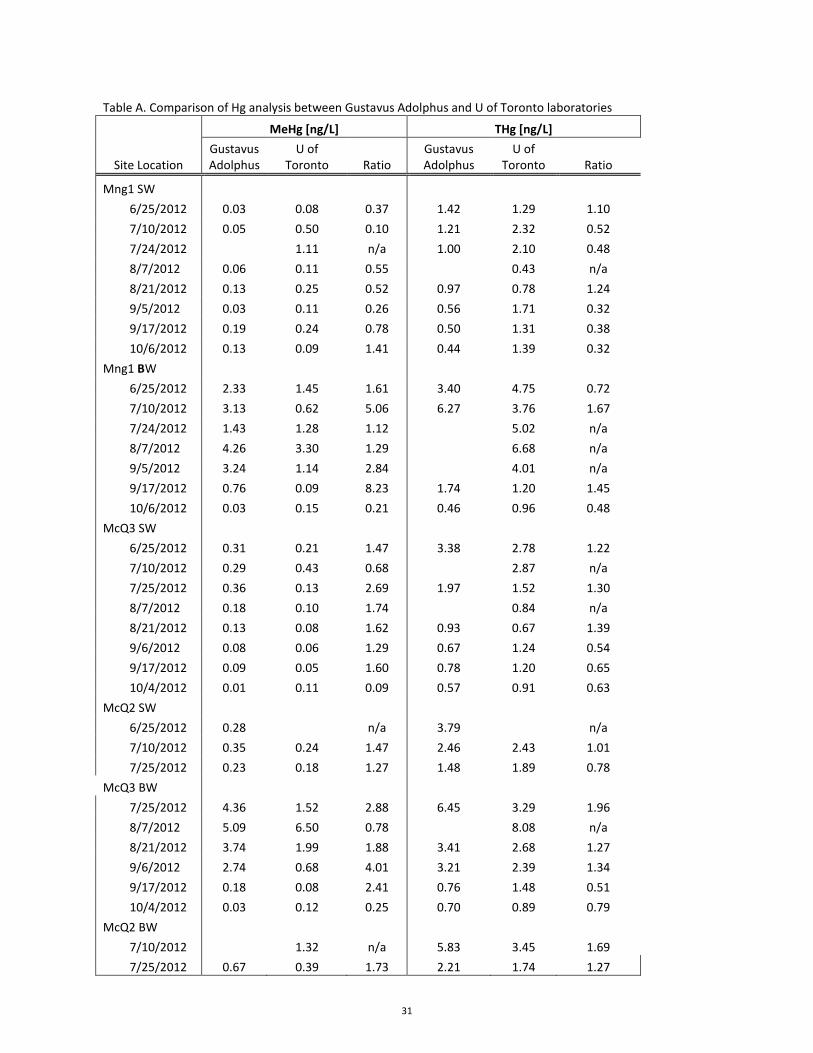
Table A. Comparison of Hg analysis between Gustavus Adolphus and U of Toronto laboratories

Site Location

MeHg [ng/L] THg [ng/L]

Gustavus Adolphus

U of Toronto Ratio

Gustavus Adolphus

U of Toronto Ratio

Mng1 SW

6/25/2012 0.03 0.08 0.37 1.42 1.29 1.10

7/10/2012 0.05 0.50 0.10 1.21 2.32 0.52

7/24/2012 1.11 n/a 1.00 2.10 0.48

8/7/2012 0.06 0.11 0.55 0.43 n/a

8/21/2012 0.13 0.25 0.52 0.97 0.78 1.24

9/5/2012 0.03 0.11 0.26 0.56 1.71 0.32

9/17/2012 0.19 0.24 0.78 0.50 1.31 0.38

10/6/2012 0.13 0.09 1.41 0.44 1.39 0.32

Mng1 BW

6/25/2012 2.33 1.45 1.61 3.40 4.75 0.72

7/10/2012 3.13 0.62 5.06 6.27 3.76 1.67

7/24/2012 1.43 1.28 1.12 5.02 n/a

8/7/2012 4.26 3.30 1.29 6.68 n/a

9/5/2012 3.24 1.14 2.84 4.01 n/a

9/17/2012 0.76 0.09 8.23 1.74 1.20 1.45

10/6/2012 0.03 0.15 0.21 0.46 0.96 0.48

McQ3 SW

6/25/2012 0.31 0.21 1.47 3.38 2.78 1.22

7/10/2012 0.29 0.43 0.68 2.87 n/a

7/25/2012 0.36 0.13 2.69 1.97 1.52 1.30

8/7/2012 0.18 0.10 1.74 0.84 n/a

8/21/2012 0.13 0.08 1.62 0.93 0.67 1.39

9/6/2012 0.08 0.06 1.29 0.67 1.24 0.54

9/17/2012 0.09 0.05 1.60 0.78 1.20 0.65

10/4/2012 0.01 0.11 0.09 0.57 0.91 0.63

McQ2 SW

6/25/2012 0.28

n/a 3.79

n/a

7/10/2012 0.35 0.24 1.47 2.46 2.43 1.01

7/25/2012 0.23 0.18 1.27 1.48 1.89 0.78

McQ3 BW

7/25/2012 4.36 1.52 2.88 6.45 3.29 1.96

8/7/2012 5.09 6.50 0.78 8.08 n/a

8/21/2012 3.74 1.99 1.88 3.41 2.68 1.27

9/6/2012 2.74 0.68 4.01 3.21 2.39 1.34

9/17/2012 0.18 0.08 2.41 0.76 1.48 0.51

10/4/2012 0.03 0.12 0.25 0.70 0.89 0.79

McQ2 BW

7/10/2012 1.32 n/a 5.83 3.45 1.69

7/25/2012 0.67 0.39 1.73 2.21 1.74 1.27

31

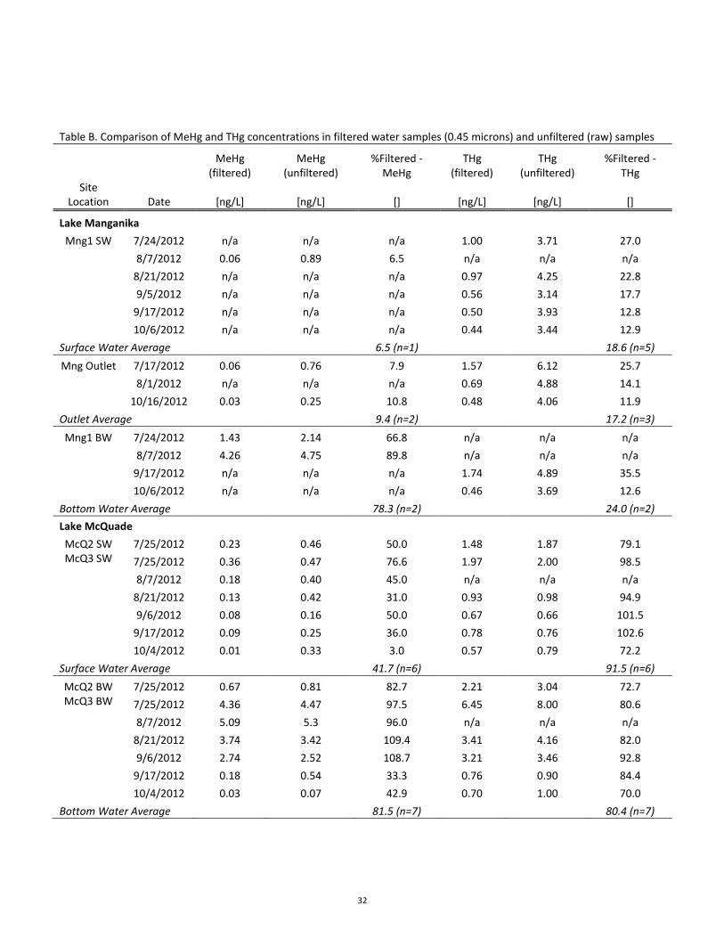
Table B. Comparison of MeHg and THg concentrations in filtered water samples (0.45 microns) and unfiltered (raw) samples

MeHg (filtered)

MeHg (unfiltered)

%Filtered -MeHg

THg (filtered)

THg (unfiltered)

%Filtered -THg

Site Location Date [ng/L] [ng/L] [] [ng/L] [ng/L] []

Lake Manganika Mng1 SW 7/24/2012 n/a n/a n/a 1.00 3.71 27.0

8/7/2012 0.06 0.89 6.5 n/a n/a n/a

8/21/2012 n/a n/a n/a 0.97 4.25 22.8

9/5/2012 n/a n/a n/a 0.56 3.14 17.7

9/17/2012 n/a n/a n/a 0.50 3.93 12.8

10/6/2012 n/a n/a n/a 0.44 3.44 12.9

Surface Water Average

6.5 (n=1)

18.6 (n=5)

Mng Outlet 7/17/2012 0.06 0.76 7.9 1.57 6.12 25.7 8/1/2012 n/a n/a n/a 0.69 4.88 14.1

10/16/2012 0.03 0.25 10.8 0.48 4.06 11.9

Outlet Average

9.4 (n=2)

17.2 (n=3)

Mng1 BW 7/24/2012 1.43 2.14 66.8 n/a n/a n/a 8/7/2012 4.26 4.75 89.8 n/a n/a n/a

9/17/2012 n/a n/a n/a 1.74 4.89 35.5

10/6/2012 n/a n/a n/a 0.46 3.69 12.6

Bottom Water Average

78.3 (n=2)

24.0 (n=2)

Lake McQuade McQ2 SW 7/25/2012 0.23 0.46 50.0 1.48 1.87 79.1

McQ3 SW 7/25/2012 0.36 0.47 76.6 1.97 2.00 98.5

8/7/2012 0.18 0.40 45.0 n/a n/a n/a

8/21/2012 0.13 0.42 31.0 0.93 0.98 94.9

9/6/2012 0.08 0.16 50.0 0.67 0.66 101.5

9/17/2012 0.09 0.25 36.0 0.78 0.76 102.6

10/4/2012 0.01 0.33 3.0 0.57 0.79 72.2

Surface Water Average

41.7 (n=6)

91.5 (n=6)

McQ2 BW 7/25/2012 0.67 0.81 82.7 2.21 3.04 72.7 McQ3 BW 7/25/2012 4.36 4.47 97.5 6.45 8.00 80.6

8/7/2012 5.09 5.3 96.0 n/a n/a n/a

8/21/2012 3.74 3.42 109.4 3.41 4.16 82.0

9/6/2012 2.74 2.52 108.7 3.21 3.46 92.8

9/17/2012 0.18 0.54 33.3 0.76 0.90 84.4

10/4/2012 0.03 0.07 42.9 0.70 1.00 70.0

Bottom Water Average 81.5 (n=7) 80.4 (n=7)

32

Table C. Measured methylation and demethylation rates for June 2013

assays

Sample Location

kmeth kdemeth MeHg THg %MeHg LDO Sulfate Sulfide Nitrate DOC

[d-1

] [hr-1

] [ng/L] [ng/L] [] [mM] [mM] [mM] [mM] [mg/L]

Mng 1 - 12.5 ft < DL < DL 0.46 2.14 21.66 0.002 6.18 0.001 0.028 5.14

Mng 1 - BW 0.009 0.014 0.94 1.07 87.98 0.000 6.75 0.176 0.017 8.45

McQ 3 - BW < DL 0.031 0.21 2.58 8.26 0.000 3.28 0.001 0.009 7.63

Table D. Estimated sediment flux of MeHg (MeHg) and inorganic mercury (iHg)

Sample Location

& Time

MeHg (BW) MeHg (0-2) MeHg Flux iHg (BW) iHg (0-2) iHg Flux

[ng/L] [ng/L] [pmol/m2/d] [ng/L] [ng/L] [pmol/m

2/d]

Mng 1 May '12 3.16 2.51 -15.8

0.12 2.86 25.2

July '12 1.28 0.69 -18.0

3.75 3.18 -5.2

October '12 0.15 2.91 70.8

0.81 5.92 47.4

June '13 0.94 1.32 9.5

0.13 41.85 391.4

Mng 2 July '12 0.10 0.38 10.3

0.86 3.79 26.9

October '12 0.09 0.15 1.3

4.47 3.43 -9.0

June '13 0.20 6.59 186.8

3.87 3.59 -2.4

McQ 2 July '12 0.39 0.54 5.0

1.35 2.81 12.9

October '12 0.07 0.33 6.7

0.92 1.80 7.4

June '13 0.21 0.65 11.6

4.02 8.51 37.6

McQ 3 July '12 1.52 1.80 8.5

1.77 2.02 2.3

October '12 0.12 0.68 15.9

0.76 2.80 18.7

June '13 0.21 1.57 38.3 2.37 10.42 72.9

33

Table E. MeHg concentrations in Lake McQuade during August lake mixing

Date Limnetic

Surface Depth Volume

(Epilimnion) Volume

(Hypolimnion) MeHg

(McQ2 SW) MeHg

(McQ3 SW) MeHg

(McQ3BW)

[ft] [m3] [m3] [ng/L] [ng/L] [ng/L]

8/7/2012 10 1.73E+06 2.72E+05 0.02 0.10 6.50

8/21/2012 11 - 12 1.84E+06 1.60E+05 0.20 0.08 1.99

MeHg (Inlet) MeHg (Outlet)

[ng/L] [ng/L] 7/31/2012 0.13 0.16 8/14/2012 0.10 0.20 8/27/2012 0.06 0.35

34

Fig. 18. Comparisons of MeHg and THg measurments between Gustavus Adolphus lab (sample filter size of 0.45 microns) and U of Toronto lab (sample filter size

of 0.2 microns

y = 0.6618x - 0.0209 R² = 0.6579

0

1

2

3

4

5

6

7

0 1 2 3 4 5 6 7

U o

f To

ron

to d

ata

[ng/

L]

Gustavus Adolphus data [ng/L]

Inter-lab MeHg Comparison

MeHg

Linear (MeHg)

y = 0.5035x + 0.1047 R² = 0.7

y = 0.7596x - 0.0832 R² = 0.6765

0

1

2

3

4

5

6

7

0 1 2 3 4 5 6 7

U o

f To

ron

to [

ng/

L]

Gustavus Adolphus data [ng/L]

Inter-lab MeHg Comparison

Mng MeHg

McQ MeHg

Linear (Mng MeHg)

Linear (McQ MeHg)

y = 0.5406x + 1.0766 R² = 0.587

y = 0.4441x + 0.8734 R² = 0.8669

0

1

2

3

4

5

0 1 2 3 4 5 6 7

U o

f To

ron

to d

ata

[ng/

L]

Gustavus Adolphus [ng/L]

Inter-lab THg Comparison

Mng THg

McQ THg

Linear (Mng THg)

Linear (McQ THg)

y = 0.4612x + 0.9913 R² = 0.6628

0

1

2

3

4

5

6

0 1 2 3 4 5 6 7

U o

f To

ron

to d

ata

[ng/

L]

Gustavus Adolphus data [ng/L]

Inter-lab THg Comparison

THg

Linear (THg)

0.0

0.5

1.0

0.0 0.5 1.00.0

0.5

1.0

0.0 0.5 1.0

35

MNG 1 (Deeper site)

Fig. 4. Time-series of Mng1 surface and bottom water samples for: (a) dissolved O2, (b) temperature, (c) sulfate, (d) nitrate, (e) sulfide and thiosulfate, (f) %MeHg, (g) MeHg, (h) iHg, (i) ferrous iron, (j)

Mg, (k) DOC & DIC, (l) conductivity, (m) SUVA, (n) pH

0

1

2

3

4

5

5/15/2012 6/14/2012 7/14/2012 8/13/2012 9/12/2012 10/12/2012

Me

Hg

[ng/

L]

BW MeHg

SW MeHg

0

1

2

3

4

5

6

5/15/2012 6/14/2012 7/14/2012 8/13/2012 9/12/2012 10/12/2012

SUV

A

BW SUVA

SW SUVA

0.0

0.4

0.8

1.2

1.6

5/15/2012 6/14/2012 7/14/2012 8/13/2012 9/12/2012 10/12/2012

Thio

sulf

ate

/Su

lfid

e [

mM

] BW SulfideSW SulfideBW Thiosulfate

-0.10

0.10

0.30

0.50

0.70

5/15/2012 6/14/2012 7/14/2012 8/13/2012 9/12/2012 10/12/2012

Dis

solv

ed

Oxy

gen

[m

M]

BW LDO

SW LDO

0.00

0.01

0.02

0.03

0.04

5/15/2012 6/14/2012 7/14/2012 8/13/2012 9/12/2012 10/12/2012

Fe (

II)

[mM

]

BW Fe(II)SW Fe(II)

0

3

6

9

12

15

0

50

100

150

200

5/15/2012 6/14/2012 7/14/2012 8/13/2012 9/12/2012 10/12/2012

DO

C [

mg/

L]

DIC

[m

g/L]

BW DICSW DICBW DOCSW DOC

6

7

8

9

10

5/15/2012 6/14/2012 7/14/2012 8/13/2012 9/12/2012 10/12/2012

pH

BW pH

SW pH

0

25

50

75

100

5/15/2012 6/14/2012 7/14/2012 8/13/2012 9/12/2012 10/12/2012

%M

eH

g []

BW %MeHg

SW %MeHg

0

5

10

15

20

25

30

5/15/2012 6/14/2012 7/14/2012 8/13/2012 9/12/2012 10/12/2012

Tem

pe

ratu

re [

de

g C

]

BW TempSW Temp

0.0

2.5

5.0

7.5

10.0

5/15/2012 6/14/2012 7/14/2012 8/13/2012 9/12/2012 10/12/2012

Mg

[mM

]

BW Mg

SW Mg

0

500

1000

1500

2000

2500

5/15/2012 6/14/2012 7/14/2012 8/13/2012 9/12/2012 10/12/2012

Co

nd

uct

ivit

y [m

S/cm

]

BW SpC

SW SpC

0

1

2

3

4

5

6

5/15/2012 6/14/2012 7/14/2012 8/13/2012 9/12/2012 10/12/2012

Sulf

ate

[m

M]

BW Sulfate

SW Sulfate

0.00

0.03

0.06

0.09

0.12

0.15

5/15/2012 6/14/2012 7/14/2012 8/13/2012 9/12/2012 10/12/2012

Nit

rate

[m

M]

BW Nitrate

SW Nitrate

0

1

2

3

4

5

5/15/2012 6/14/2012 7/14/2012 8/13/2012 9/12/2012 10/12/2012

iHg

[ng/

L]

BW iHg

SW iHg

(h)

(j) (i)

(k) (l)

(n) (m)

(a)

(d) (c)

(b)

(g)

(e) (f)

36

MNG 2 (Shallower site)

Fig. 5. Time-series of Mng2 surface and bottom water samples for: (a) dissolved O2, (b) temperature, (c) sulfate, (d) nitrate, (e) sulfide, (f) %MeHg, (g) MeHg, (h) inorganic-Hg, (i) ferrous iron, (j) DOC & DIC,

(k) conductivity, (l) pH

0

1

2

3

4

5

5/15/2012 6/14/2012 7/14/2012 8/13/2012 9/12/2012 10/12/2012

iHg

[ng/

L]

BW iHg

SW iHg

0.00

0.01

0.02

0.03

0.04

5/15/2012 6/14/2012 7/14/2012 8/13/2012 9/12/2012 10/12/2012

Fe (

II)

[mM

]

BW Fe(II)SW Fe(II)

0

3

6

9

12

15

0

50

100

150

200

5/15/2012 6/14/2012 7/14/2012 8/13/2012 9/12/2012 10/12/2012

DO

C [

mg/

L]

DIC

[m

g/L]

BW DICSW DICBW DOCSW DOC

0

1

2

3

4

5

6

5/15/2012 6/14/2012 7/14/2012 8/13/2012 9/12/2012 10/12/2012

Sulf

ate

[m

M]

BW Sulfate

SW Sulfate

0

1

2

3

4

5

6

5/15/2012 6/14/2012 7/14/2012 8/13/2012 9/12/2012 10/12/2012

Sulf

ate

[m

M]

BW Sulfate

SW Sulfate

(c)

(h)

(j) (i)

0.000

0.001

0.002

0.003

0.004

0.005

5/15/2012 6/14/2012 7/14/2012 8/13/2012 9/12/2012 10/12/2012

Sulf

ide

[m

M]

BW Sulfide

SW Sulfide

(e) 0

25

50

75

100

5/15/2012 6/14/2012 7/14/2012 8/13/2012 9/12/2012 10/12/2012

%M

eH

g []

BW %MeHg

SW %MeHg

(f)

0.00

0.03

0.06

0.09

0.12

0.15

5/15/2012 6/14/2012 7/14/2012 8/13/2012 9/12/2012 10/12/2012

Nit

rate

[m

M]

BW Nitrate

SW Nitrate

(d)

0

1

2

3

4

5

5/15/2012 6/14/2012 7/14/2012 8/13/2012 9/12/2012 10/12/2012

Me

Hg

[ng/

L]

BW MeHg

SW MeHg

(g)

0

400

800

1200

1600

2000

5/15/2012 6/14/2012 7/14/2012 8/13/2012 9/12/2012 10/12/2012

Co

nd

uct

ivit

y [m

S/cm

]

BW SpCSW SpC

6

7

8

9

10

5/15/2012 6/14/2012 7/14/2012 8/13/2012 9/12/2012 10/12/2012

pH

BW pHSW pH

(k) (l)

-0.10

0.10

0.30

0.50

0.70

5/15/2012 6/14/2012 7/14/2012 8/13/2012 9/12/2012 10/12/2012

Dis

solv

ed

Oxy

gen

[m

M]

BW LDO

SW LDO

(a) 0

5

10

15

20

25

30

5/15/2012 6/14/2012 7/14/2012 8/13/2012 9/12/2012 10/12/2012

Tem

pe

ratu

re [

de

g C

]

BW TempSW Temp

(b)

37

Fig. 6. Lake Manganika temperature profiles, taken biweekly at both sampling locations

0

6

12

18

24

8.0 12.0 16.0 20.0 24.0 28.0

De

pth

[ft

]

Temp [C]

(a) - 6/5

Mng 1

Mng 2

0

6

12

18

24

8 12 16 20 24 28

De

pth

[ft

]

Temp [C]

(e) - 8/7

Mng 1

Mng 2

0

6

12

18

24

8 12 16 20 24 28

De

pth

[ft

]

Temp [C]

(b) - 6/25

Mng 1

Mng 2

0

6

12

18

24

8 12 16 20 24 28

De

pth

[ft

]

Temp [C]

(c) - 7/10

Mng 1

Mng 2

0

6

12

18

24

8 12 16 20 24 28

De

pth

[ft

]

Temp [C]

(d) - 7/24

Mng 1

Mng 2

0

6

12

18

24

8 12 16 20 24 28

De

pth

[ft

]

Temp [C]

(f) - 8/21

Mng 1

Mng 2

0

6

12

18

24

8 12 16 20 24 28

De

pth

[ft

]

Temp [C]

(g) - 9/17

Mng 1

Mng 2

0

6

12

18

24

8 12 16 20 24 28

De

pth

[ft

]

Temp [C]

(h) - 10/6

Mng 1

Mng 2

38

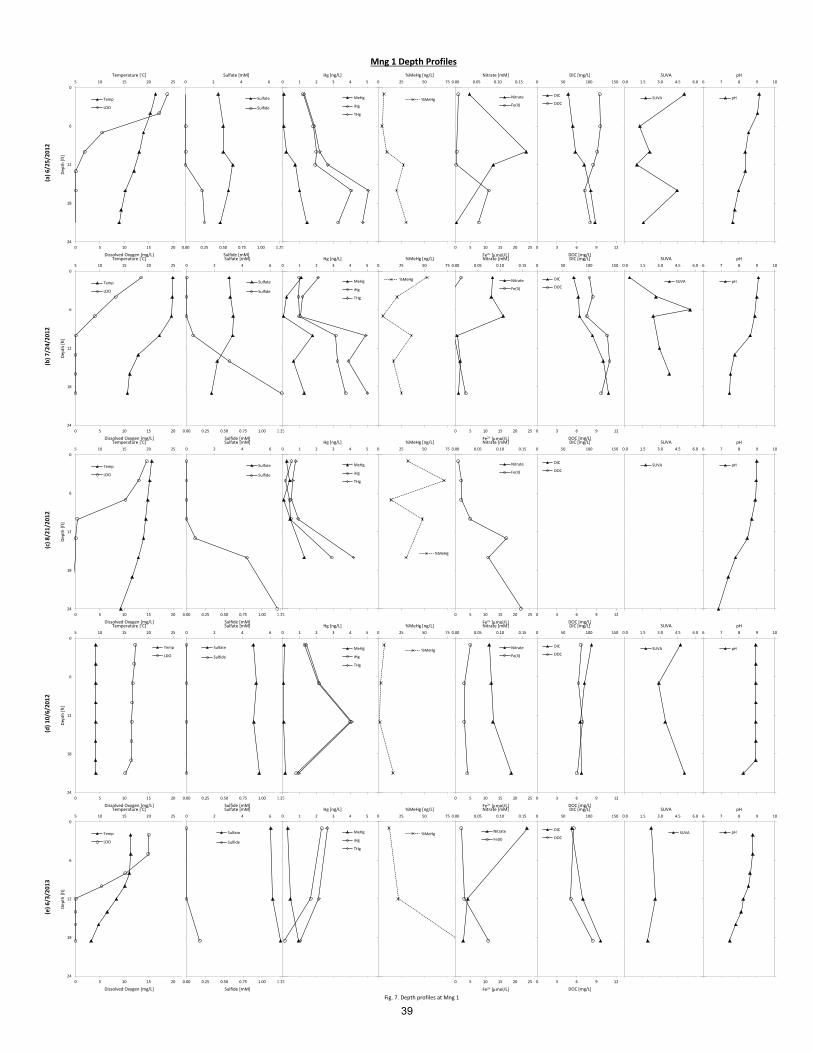
Fig. 7. Depth profiles at Mng 1

(d)

10

/6/2

01

2(e

) 6

/3/2

01

3

Mng 1 Depth Profiles

(a)

6/2

5/2

01

2(b

) 7

/24

/20

12

(c)

8/2

1/2

01

2

0.00 0.25 0.50 0.75 1.00 1.25

0

6

12

18

24

0 2 4 6

Sulfide [mM]

Sulfate [mM]

Sulfate

Sulfide

0.00 0.25 0.50 0.75 1.00 1.25

0

6

12

18

24

0 2 4 6

Sulfide [mM]

Sulfate [mM]

Sulfate

Sulfide

0.00 0.25 0.50 0.75 1.00 1.25

0

6

12

18

24

0 2 4 6

Sulfide [mM]

Sulfate [mM]

Sulfate

Sulfide

0 5 10 15 20

0

6

12

18

24

5 10 15 20 25

Dissolved Oxygen [mg/L]

Dep

th [

ft]

Temperature [◦C]

Temp

LDO

0.00 0.25 0.50 0.75 1.00 1.25

0

6

12

18

24

0 2 4 6

Sulfide [mM]

Sulfate [mM]

Sulfate

Sulfide

0.00 1.00 2.00 3.00 4.00 5.00

0

6

12

18

24

0 1 2 3 4 5

Hg [ng/L]

MeHg

iHg

THg

0.00 25.00 50.00 75.00

0

6

12

18

24

0 25 50 75

%MeHg [ng/L]

%MeHg

0 5 10 15 20 25

0

6

12

18

24

0.00 0.05 0.10 0.15

Fe2+ [mmol/L]

Nitrate [mM]

Nitrate

Fe(II)

0 3 6 9 12

0

6

12

18

24

0 50 100 150

DOC [mg/L]

DIC [mg/L]

DIC

DOC

0.00 1.50 3.00 4.50 6.00

0

6

12

18

24

0.0 1.5 3.0 4.5 6.0

SUVA

SUVA

6.00 7.00 8.00 9.00 10.00

0

6

12

18

24

0

6

12

18

24

6 7 8 9 10

pH

pH

0 5 10 15 20

0

6

12

18

24

5 10 15 20 25

Dissolved Oxygen [mg/L]

Dep

th [

ft]

Temperature [◦C]

Temp

LDO

0.00 25.00 50.00 75.00

0

6

12

18

24

0 25 50 75

%MeHg [ng/L]

%MeHg

0 5 10 15 20 25

0

6

12

18

24

0.00 0.05 0.10 0.15

Fe2+ [mmol/L]

Nitrate [mM]

Nitrate

Fe(II)

0 3 6 9 12

0

6

12

18

24

0 50 100 150

DOC [mg/L]

DIC [mg/L]

DIC

DOC

0.00 1.50 3.00 4.50 6.00

0

6

12

18

24

0.0 1.5 3.0 4.5 6.0

SUVA

SUVA

6.00 7.00 8.00 9.00 10.00

0

6

12

18

24

0

6

12

18

24

6 7 8 9 10

pH

pH

0 5 10 15 20

0

6

12

18

24

5 10 15 20 25

Dissolved Oxygen [mg/L]

Dep

th [

ft]

Temperature [◦C]

Temp

LDO

0.00 1.00 2.00 3.00 4.00 5.00

0

6

12

18

24

0 1 2 3 4 5

Hg [ng/L]

MeHg

iHg

THg

0.00 25.00 50.00 75.00

0

6

12

18

24

0 25 50 75

%MeHg [ng/L]

%MeHg

0 5 10 15 20 25

0

6

12

18

24

0.00 0.05 0.10 0.15

Fe2+ [mmol/L]

Nitrate [mM]

Nitrate

Fe(II)

0 3 6 9 12

0

6

12

18

24

0 50 100 150

DOC [mg/L]

DIC [mg/L]

DIC

DOC

0.00 1.50 3.00 4.50 6.00

0

6

12

18

24

0.0 1.5 3.0 4.5 6.0

SUVA

SUVA

6.00 7.00 8.00 9.00 10.00

0

6

12

18

24

0

6

12

18

24

6 7 8 9 10

pH

pH

0 5 10 15 20

0

6

12

18

24

5 10 15 20 25

Dissolved Oxygen [mg/L]

Dep

th [

ft]

Temperature [◦C]

Temp

LDO

0.00 1.00 2.00 3.00 4.00 5.00

0

6

12

18

24

0 1 2 3 4 5

Hg [ng/L]

MeHg

iHg

THg

0.00 25.00 50.00 75.00

0

6

12

18

24

0 25 50 75

%MeHg [ng/L]

%MeHg

0 5 10 15 20 25

0

6

12

18

24

0.00 0.05 0.10 0.15

Fe2+ [mmol/L]

Nitrate [mM]

Nitrate

Fe(II)

0 3 6 9 12

0

6

12

18

24

0 50 100 150

DOC [mg/L]

DIC [mg/L]

DIC

DOC

0.00 1.50 3.00 4.50 6.00

0

6

12

18

24

0.0 1.5 3.0 4.5 6.0

SUVA

SUVA

6.00 7.00 8.00 9.00 10.00

0

6

12

18

24

0

6

12

18

24

6 7 8 9 10

pH

pH

0 5 10 15 20

0

6

12

18

24

5 10 15 20 25

Dissolved Oxygen [mg/L]

Dep

th [

ft]

Temperature [◦C]

Temp

LDO

0.00 1.00 2.00 3.00 4.00 5.00

0

6

12

18

24

0 1 2 3 4 5

Hg [ng/L]

MeHg

iHg

THg

0.00 25.00 50.00 75.00

0

6

12

18

24

0 25 50 75

%MeHg [ng/L]

%MeHg

0 5 10 15 20 25

0

6

12

18

24

0.00 0.05 0.10 0.15

Fe2+ [mmol/L]

Nitrate [mM]

Nitrate

Fe(II)

0 3 6 9 12

0

6

12

18

24

0 50 100 150

DOC [mg/L]

DIC [mg/L]

DIC

DOC

0.00 1.50 3.00 4.50 6.00

0

6

12

18

24

0.0 1.5 3.0 4.5 6.0

SUVA

SUVA

6.00 7.00 8.00 9.00 10.00

0

6

12

18

24

0

6

12

18

24

6 7 8 9 10

pH

pH

0.00 0.25 0.50 0.75 1.00 1.25

0

6

12

18

24

0 2 4 6

Sulfide [mM]

Sulfate [mM]

Sulfate

Sulfide

0.00 1.00 2.00 3.00 4.00 5.00

0

6

12

18

24

0 1 2 3 4 5

Hg [ng/L]

MeHg

iHg

THg

39

MNG Inlet & Outlet

Fig. 8. Time-series of Lake Manganika inlet and outlet streams for: (a) MeHg, (b) THg, (c) %MeHg, (d) conductivity, (e) sulfate (f) nitrate, (g) Mg

0

1

2

3

4

5

5/15/2012 6/14/2012 7/14/2012 8/13/2012 9/12/2012 10/12/2012

THg

[ng/

L]

0

1

2

3

4

5/15/2012 6/14/2012 7/14/2012 8/13/2012 9/12/2012 10/12/2012

Me

Hg

[ng/

L]

Mng Inlet (Mine)

Mng Inlet (WWTP)

Mng Outlet

0

20

40

60

80

100

5/15/2012 6/14/2012 7/14/2012 8/13/2012 9/12/2012 10/12/2012

%M

eH

g []

0.00

0.15

0.30

0.45

0.60

0.75

5/15/2012 6/14/2012 7/14/2012 8/13/2012 9/12/2012 10/12/2012

Nit

rate

[m

M]

0

2

4

6

8

5/15/2012 6/14/2012 7/14/2012 8/13/2012 9/12/2012 10/12/2012

Sulf

ate

[m

M]

0

500

1000

1500

2000

2500

5/15/2012 6/14/2012 7/14/2012 8/13/2012 9/12/2012 10/12/2012

Co

nd

uct

ivit

y [m

S/cm

]

0

2

4

6

8

10

12

5/15/2012 6/14/2012 7/14/2012 8/13/2012 9/12/2012 10/12/2012

Mg

[mM

]

(a)

(e) (b)

(d)

(c) (f)

(g)

40

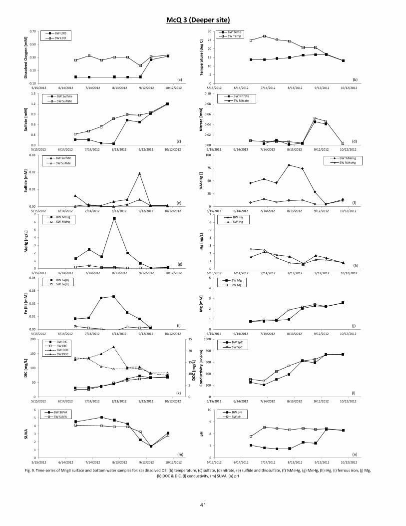
McQ 3 (Deeper site)

Fig. 9. Time-series of Mng3 surface and bottom water samples for: (a) dissolved O2, (b) temperature, (c) sulfate, (d) nitrate, (e) sulfide and thiosulfate, (f) %MeHg, (g) MeHg, (h) iHg, (i) ferrous iron, (j) Mg,

(k) DOC & DIC, (l) conductivity, (m) SUVA, (n) pH

0

1

2

3

4

5

6

7

5/15/2012 6/14/2012 7/14/2012 8/13/2012 9/12/2012 10/12/2012

Me

Hg

[ng/

L]

BW MeHg

SW MeHg

0

1

2

3

4

5

6

5/15/2012 6/14/2012 7/14/2012 8/13/2012 9/12/2012 10/12/2012

SUV

A

BW SUVA

SW SUVA

0.00

0.01

0.02

0.03

5/15/2012 6/14/2012 7/14/2012 8/13/2012 9/12/2012 10/12/2012

Sulf

ide

[m

M]

BW Sulfide

SW Sulfide

-0.10

0.10

0.30

0.50

0.70

5/15/2012 6/14/2012 7/14/2012 8/13/2012 9/12/2012 10/12/2012

Dis

solv

ed

Oxy

gen

[m

M]

BW LDO

SW LDO

0.00

0.01

0.02

0.03

0.04

5/15/2012 6/14/2012 7/14/2012 8/13/2012 9/12/2012 10/12/2012

Fe (

II)

[mM

]

BW Fe(II)SW Fe(II)

0

5

10

15

20

25

0

50

100

150

200

5/15/2012 6/14/2012 7/14/2012 8/13/2012 9/12/2012 10/12/2012

DO

C [

mg/

L]

DIC

[m

g/L]

BW DICSW DICBW DOCSW DOC

6

7

8

9

10

5/15/2012 6/14/2012 7/14/2012 8/13/2012 9/12/2012 10/12/2012

pH

BW pH

SW pH

0

25

50

75

100

5/15/2012 6/14/2012 7/14/2012 8/13/2012 9/12/2012 10/12/2012

%M

eH

g []

BW %MeHg

SW %MeHg

0

5

10

15

20

25

30

5/15/2012 6/14/2012 7/14/2012 8/13/2012 9/12/2012 10/12/2012

Tem

pe

ratu

re [

de

g C

]

BW TempSW Temp

0

1

2

3

4

5

5/15/2012 6/14/2012 7/14/2012 8/13/2012 9/12/2012 10/12/2012

Mg

[mM

]

BW Mg

SW Mg

0

200

400

600

800

1000

5/15/2012 6/14/2012 7/14/2012 8/13/2012 9/12/2012 10/12/2012

Co

nd

uct

ivit

y [m

S/cm

]

BW SpC

SW SpC

0.0

0.3

0.6

0.9

1.2

1.5

5/15/2012 6/14/2012 7/14/2012 8/13/2012 9/12/2012 10/12/2012

Sulf

ate

[m

M]

BW Sulfate

SW Sulfate

0.00

0.02

0.04

0.06

0.08

0.10

5/15/2012 6/14/2012 7/14/2012 8/13/2012 9/12/2012 10/12/2012

Nit

rate

[m

M]

BW Nitrate

SW Nitrate

0

1

2

3

4

5

6

7

5/15/2012 6/14/2012 7/14/2012 8/13/2012 9/12/2012 10/12/2012

iHg

[ng/

L]

BW iHg

SW iHg

(h)

(j) (i)

(k) (l)

(n) (m)

(a)

(d) (c)

(b)

(g)

(e) (f)

41

McQ 2 (Shallower site)

Fig. 10. Time-series of McQ2 surface and bottom water samples for: (a) dissolved O2, (b) temperature, (c) sulfate, (d) nitrate, (e) sulfide and thiosulfate, (f) %MeHg, (g) MeHg, (h) iHg, (i) ferrous iron, (j)

Conductivity (k) DIC, (l) DOC, (m) SUVA, (n) pH

0

1

2

3

4

5

6

7

5/15/2012 6/14/2012 7/14/2012 8/13/2012 9/12/2012 10/12/2012

Me

Hg

[ng/

L]

BW MeHg

SW MeHg

0

1

2

3

4

5

6

5/15/2012 6/14/2012 7/14/2012 8/13/2012 9/12/2012 10/12/2012

SUV

A

BW SUVA

SW SUVA

0.00

0.01

0.02

0.03

5/15/2012 6/14/2012 7/14/2012 8/13/2012 9/12/2012 10/12/2012

Sulf

ide

[m

M]

BW Sulfide

SW Sulfide

-0.10

0.10

0.30

0.50

0.70

5/15/2012 6/14/2012 7/14/2012 8/13/2012 9/12/2012 10/12/2012

Dis

solv

ed

Oxy

gen

[m

M]

BW LDO

SW LDO

0.00

0.01

0.02

0.03

0.04

5/15/2012 6/14/2012 7/14/2012 8/13/2012 9/12/2012 10/12/2012

Fe (

II)

[mM

]

BW Fe(II)SW Fe(II)

0

25

50

75

100

5/15/2012 6/14/2012 7/14/2012 8/13/2012 9/12/2012 10/12/2012

DIC

[m

g/L]

BW DIC

SW DIC

6

7

8

9

10

5/15/2012 6/14/2012 7/14/2012 8/13/2012 9/12/2012 10/12/2012

pH

BW pH

SW pH

0

25

50

75

100

5/15/2012 6/14/2012 7/14/2012 8/13/2012 9/12/2012 10/12/2012

%M

eH

g []

BW %MeHg

SW %MeHg

0

5

10

15

20

25

30

5/15/2012 6/14/2012 7/14/2012 8/13/2012 9/12/2012 10/12/2012

Tem

pe

ratu

re [

de

g C

]

BW TempSW Temp

0

200

400

600

800

1000

5/15/2012 6/14/2012 7/14/2012 8/13/2012 9/12/2012 10/12/2012

Co

nd

uct

ivit

y [m

S/cm

]

BW SpC

SW SpC

0

5

10

15

20

25

5/15/2012 6/14/2012 7/14/2012 8/13/2012 9/12/2012 10/12/2012

DO

C [

mg/

L]

BW DOC

SW DOC

0.0

0.3

0.6

0.9

1.2

1.5

5/15/2012 6/14/2012 7/14/2012 8/13/2012 9/12/2012 10/12/2012

Sulf

ate

[m

M]

BW Sulfate

SW Sulfate

0.00

0.02

0.04

0.06

0.08

0.10

5/15/2012 6/14/2012 7/14/2012 8/13/2012 9/12/2012 10/12/2012

Nit

rate

[m

M]

BW Nitrate

SW Nitrate

0

1

2

3

4

5

6

7

5/15/2012 6/14/2012 7/14/2012 8/13/2012 9/12/2012 10/12/2012

iHg

[ng/

L]

BW iHg

SW iHg

(h)

(j) (i)

(k) (l)

(n) (m)

(a)

(d) (c)

(b)

(g)

(e) (f)

42

Fig. 11. Lake McQuade temperature profiles, taken biweekly at both sampling locations

0

3

6

9

12

15

8 12 16 20 24 28

De

pth

[ft

]

Temp [C]

(a) - 6/5

McQ 3

McQ 2

0

3

6

9

12

15

8 12 16 20 24 28

De

pth

[ft

]

Temp [C]

McQ 3

McQ 2

0

3

6

9

12

15

8 12 16 20 24 28

De

pth

[ft

]

Temp [C]

McQ 3

McQ 2

0

3

6

9

12

15

8 12 16 20 24 28

De

pth

[ft

]

Temp [C]

McQ 3

McQ 2

0

3

6

9

12

15

8 12 16 20 24 28

De

pth

[ft

]

Temp [C]

McQ 3

McQ 2

0

3

6

9

12

15

8 12 16 20 24 28

De

pth

[ft

]

Temp [C]

McQ 3

McQ 2

0

3

6

9

12

15

8 12 16 20 24 28

De

pth

[ft

]

Temp [C]

McQ 3

McQ 2

(b) - 6/25

(e) - 8/21 (d) - 8/7 (f) - 9/17

(c) - 7/10

(g) - 10/6

43

McQ 3 Depth Profiles

6/2

5/2

01

27

/24

/20

12

8/2

1/2

01

21

0/6

/20

12

Fig. 12. Depth profiles at McQ 3

0 5 10 15

0

3

6

9

12

15

5 10 15 20 25

Dissolved Oxygen [mg/L]

Dep

th [

ft]

Temperature [◦C]

Temp

LDO

0.00 25.00 50.00 75.00

0

3

6

9

12

15

0 25 50 75

%MeHg [ng/L]

%MeHg

0 5 10 15 20 25

0

3

6

9

12

15

0.00 0.05 0.10 0.15

Fe2+ [mmol/L]

Nitrate [mM]

Nitrate

Fe(II)

0 5 10 15 20

0

3

6

9

12

15

0 15 30 45 60 75

DOC [mg/L]

DIC [mg/L]

DIC

DOC

0.00 1.50 3.00 4.50 6.00

0

3

6

9

12

15

0.0 1.5 3.0 4.5 6.0

SUVA

SUVA

6.00 7.00 8.00 9.00 10.00

0

3

6

9

12

15

0

3

6

9

12

15

6 7 8 9 10

pH

pH

0 5 10 15

0

3

6

9

12

15

5 10 15 20 25

Dissolved Oxygen [mg/L]

Dep

th [

ft]

Temperature [◦C]

Temp LDO

0.00 25.00 50.00 75.00

0

3

6

9

12

15

0 25 50 75

%MeHg [ng/L]

%MeHg

0 5 10 15 20 25

0

3

6

9

12

15

0.00 0.05 0.10 0.15

Fe2+ [mmol/L]

Nitrate [mM]

Nitrate

Fe(II)

0 5 10 15 20

0

3

6

9

12

15

0 15 30 45 60 75

DOC [mg/L]

DIC [mg/L]

DIC

DOC

0.00 1.50 3.00 4.50 6.00

0

3

6

9

12

15

0.0 1.5 3.0 4.5 6.0

SUVA

SUVA

6.00 7.00 8.00 9.00 10.00

0

3

6

9

12

15

0

3

6

9

12

15

6 7 8 9 10

pH

pH

0 5 10 15

0

3

6

9

12

15

5 10 15 20 25

Dissolved Oxygen [mg/L]

Dep

th [

ft]

Temperature [◦C]

Temp

LDO

0.000 0.005 0.010 0.015 0.020 0.025

0

3

6

9

12

15

0.0 0.3 0.6 0.9 1.2

Sulfide [mM]

Sulfate [mM]

Sulfate

Sulfide

0.00 1.00 2.00 3.00 4.00 5.00

0

3

6

9

12

15

0 1 2 3 4 5

Hg [ng/L]

MeHg

iHg

THg

0.00 25.00 50.00 75.00

0

3

6

9

12

15

0 25 50 75

%MeHg [ng/L]

%MeHg

0 5 10 15 20 25

0

3

6

9

12

15

0.00 0.05 0.10 0.15

Fe2+ [mmol/L]

Nitrate [mM]

Nitrate

Fe(II)

0 5 10 15 20

0

3

6

9

12

15

0 15 30 45 60 75

DOC [mg/L]

DIC [mg/L]

DIC

DOC

0.00 1.50 3.00 4.50 6.00

0

3

6

9

12

15

0.0 1.5 3.0 4.5 6.0

SUVA

SUVA

6.00 7.00 8.00 9.00 10.00

0

3

6

9

12

15

0

3

6

9

12

15

6 7 8 9 10

pH

pH

0 5 10 15

0

3

6

9

12

15

5 10 15 20 25

Dissolved Oxygen [mg/L]

Dep

th [

ft]

Temperature [◦C]

Temp

LDO

0.00 25.00 50.00 75.00

0

3

6

9

12

15

0 25 50 75

%MeHg [ng/L]

%MeHg

0 5 10 15 20 25

0

3

6

9

12

15

0.00 0.05 0.10 0.15

Fe2+ [mmol/L]

Nitrate [mM]

Nitrate

Fe(II)

0 5 10 15 20

0

3

6

9

12

15

0 15 30 45 60 75

DOC [mg/L]

DIC [mg/L]

DIC

DOC

0.00 1.50 3.00 4.50 6.00

0

3

6

9

12

15

0.0 1.5 3.0 4.5 6.0

SUVA

SUVA

6.00 7.00 8.00 9.00 10.00

0

3

6

9

12

15

0

3

6

9

12

15

6 7 8 9 10

pH

pH

0.000 0.005 0.010 0.015 0.020 0.025

0

3

6

9

12

15

0.0 0.3 0.6 0.9 1.2

Sulfide [mM]

Sulfate [mM]

Sulfate

Sulfide

0.00 1.00 2.00 3.00 4.00 5.00

0

3

6

9

12

15

0 1 2 3 4 5

Hg [ng/L]

MeHg

iHg

THg

0.000 0.005 0.010 0.015 0.020 0.025

0

3

6

9

12

15

0.0 0.3 0.6 0.9 1.2

Sulfide [mM]

Sulfate [mM]

Sulfate

Sulfide

0.00 1.00 2.00 3.00 4.00 5.00

0

3

6

9

12

15

0 1 2 3 4 5

Hg [ng/L]

MeHg

iHg

THg

0.000 0.005 0.010 0.015 0.020 0.025

0

3

6

9

12

15

0.0 0.3 0.6 0.9 1.2

Sulfide [mM]

Sulfate [mM]

Sulfate

Sulfide

0.00 1.00 2.00 3.00 4.00 5.00

0

3

6

9

12

15

0 1 2 3 4 5

Hg [ng/L]

MeHg

iHg

THg

44

McQ Inlet & Outlet

Fig. 13. Time-series of Lake McQuade inlet and outlet streams for: (a) MeHg, (b) THg, (c) %MeHg, (d) conductivity, (e) sulfate (f) nitrate, (g) Mg

(a)

(e) (b)

(d)

(c) (f)

(g)

0.0

0.5

1.0

5/15/2012 6/14/2012 7/14/2012 8/13/2012 9/12/2012 10/12/2012

Me

Hg

[ng/

L]

McQ Inlet

McQ Outlet

0

1

2

3

4

5/15/2012 6/14/2012 7/14/2012 8/13/2012 9/12/2012 10/12/2012

THg

[ng/

L]

0

10

20

30

40

50

60

5/15/2012 6/14/2012 7/14/2012 8/13/2012 9/12/2012 10/12/2012

% M

eH

g []

0.00

0.10

0.20

0.30

0.40

0.50

5/15/2012 6/14/2012 7/14/2012 8/13/2012 9/12/2012 10/12/2012

Nit

rate

[m

M]

0.0

0.5

1.0

1.5

2.0

5/15/2012 6/14/2012 7/14/2012 8/13/2012 9/12/2012 10/12/2012

Sulf

ate

[m

M]

0

200

400

600

800

1000

5/15/2012 6/14/2012 7/14/2012 8/13/2012 9/12/2012 10/12/2012

Co

nd

uct

ivit

y [m

S/cm

]

0

1

2

3

4

5/15/2012 6/14/2012 7/14/2012 8/13/2012 9/12/2012 10/12/2012

Mg

[mM

]

45

Fig. 14a. (left) DOC concntrations in inlet and outlet streams over summer and fall 2012

Fig. 14b. (right) MeHg and DOC concentrations of inlet and outlet water samples

Fig. 15. Estimated flux of MeHg from Lake McQuade sediment

0

5

10

15

20

5/15/2012 6/14/2012 7/14/2012 8/13/2012 9/12/2012 10/12/2012

DO

C [

mg/

L]

McQ Inlet

McQ Outlet

y = 0.0349x - 0.1555 R² = 0.7364

y = 0.0358x - 0.2527 R² = 0.6582

0.00

0.10

0.20

0.30

0.40

0.50

0.60

0.0 5.0 10.0 15.0 20.0 25.0

Me

Hg

[ng/

L]

DOC [mg/L]

McQ Inlet

McQ Outlet

Linear (McQ Inlet)

Linear (McQ Outlet)

0

10

20

30

40

McQ 2 McQ 3

Me

Hg

Flu

x [p

mo

l/m

2 /d

] July '12

Oct '12June '13

46

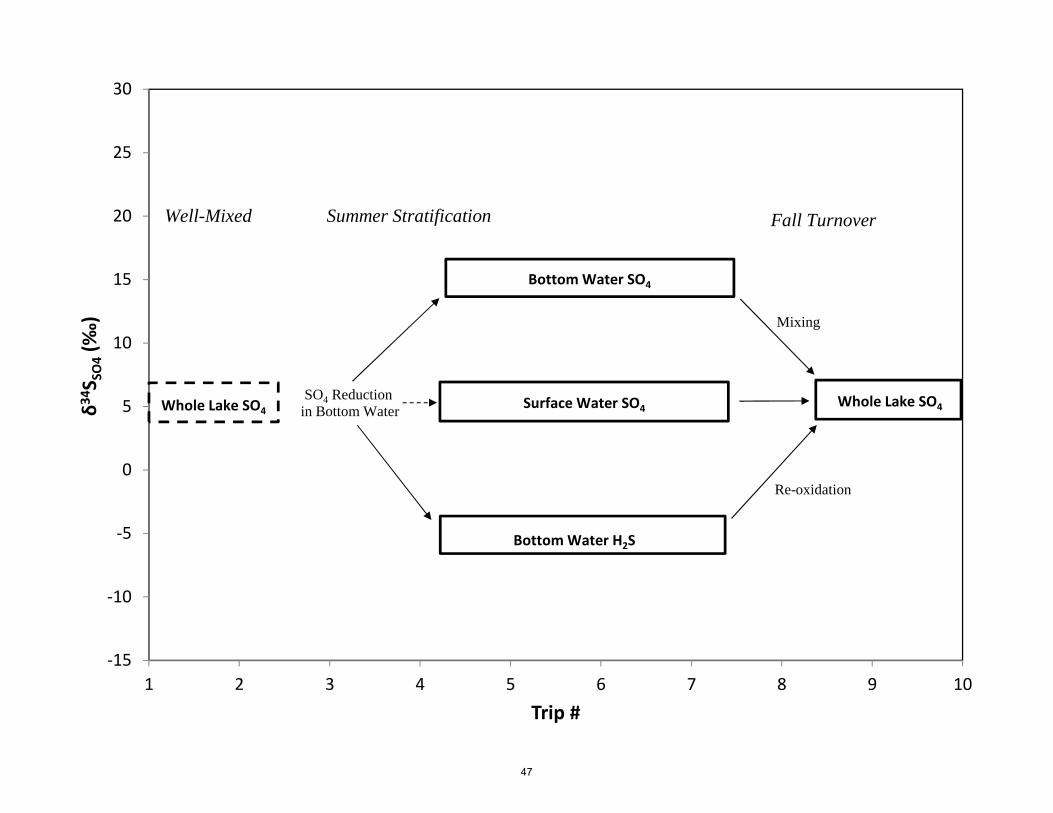
‐15

‐10

‐5

0

5

10

15

20

25

30

1 2 3 4 5 6 7 8 9 10

δ34 S

SO4(‰

)

Trip #

Surface Water SO4

Fall TurnoverSummer StratificationWell-Mixed

SO4 Reduction in Bottom Water

Bottom Water SO4

Bottom Water H2S

Whole Lake SO4

Re-oxidation

Whole Lake SO4

Mixing

47

-6

-5

-4

-3

-2

-1

0

1

2

3

4

5

6

4 5 6 7 8 9 10 11 12 13 14

δ18 O

(‰)

δ34S (‰)

Upstream McQuade

Downstream McQuade

McQuade Surface

McQuade Bottom

WTR Downstream of Res

WTR Confluence

5

6

10

9

8

7

10

10

10

10

85

679

5

7

69

8

108

9

7 8

5

9

876

9

57

6

10 ‐ Oct 49 ‐ Sept 178 ‐ Sept 67 ‐ Aug 216 ‐ Aug 75‐ Jul 2(streams  sampled 1 week later)

48

49

Appendix A: Draft reactive transport model for sulfate and MeHg in McQuade Lake Based on a mass balance on only the well-mixed epilimnion of a lake, the transient change in the concentration of a constituent can be described by:

ACkCQQCdt

dCV mtin

Where

- kmt is the mass transfer coefficient for a first-order, areal mass transport process out of the epilimnion

- Cin is the concentration in the inlet stream - Q is the inlet and outlet flow - V is the epilimnetic volume - A is the area of the limnetic surface - C is the concentration in the well-mixed epilimnion

The steady state solution to this equation is:

And the transient response to a step up in concentration from C0 to a new Cin is given by:

Assuming negligible mass transport of magnesium across the limnetic surface (no consumption in

bottom waters / sediment), the residence time (τ) can be adjusted to match concentrations at the

outlet. A residence time of 45-60 days provided a reasonable estimate of the response in outlet Mg

concentrations following the step up in inlet Mg in early July. (A MORE COMPLETE MODEL INCLUDING

THE HYPOLIMNON LAKE VOLUME – AND MASS TRANSFER RESISTANCES ASSOCIATED WITH IT – IS

UNDER DEVELOPMENT).

Q

Ak

CC

mt

inss

1

t

Q

Ak

ssss

mt

eCCCtC

1

0

50

Figure A1 Observed and modeled epilimnetic concentrations of (a) magnesium, and (b) sulfate for Lake

McQuade during summer 2012.

With an estimate for τ, an estimate for kmt can be made to describe the mass transport of sulfate out of

the epilimnion by fitting to outlet sulfate concentrations. The estimated mass transfer coefficient that

matched observed outlet sulfate concentrations was 0.0087 m/day. This net mass transport coefficient,

describes the flux of sulfate from the aerobic epilimnion to the anoxic areas of sulfate reduction (either

in hypolimnion or sediments). Since sulfate reduction typically occurs concomitantly with mercury

methylation, the same effective mass transfer coefficient could be used to estimate the rate of mass

transport in the opposite direction, e.g. for MeHg from anoxic areas to the oxidized epilimnion.

When similarly applied to the difference between hypolimnion/porewater and epilimnion MeHg

concentrations for the mid-summer, this effective mass transfer coefficient leads to an estimate of a flux

of 14.5 mg/day to the epilimnion during the peak summer months.

ACCkFAmMeHg

epi

MeHg

shmthypo /

Ch/s = 2.75 ng/L Cepi = 0.25 ng/L A = 0.67 km2 kmt = 0.0087 / day

0

10

20

30

40

50

60

70

80

90

100

5/15 6/24 8/3 9/12 10/22

[mg/

L]

McQ Outlet Modeled Magnesium

McQ mg outlet

McQ Mg inlet

C(t)|Mg

C(t)|Mginlet

0

20

40

60

80

100

120

140

160

180

5/15 6/24 8/3 9/12 10/22

[mg/

L]

McQ Outlet Modeled Sulfate

McQ Inlet [Sulfate]McQ Outlet [Sulfate]C(t)|SO4inletC(t)|SO4

C(t)|SO4ss

51

The flux out of the lake during mid-summer based on outlet concentrations and flow estimated from

average residence time represents 9.7 mg/day, suggesting demethylation of MeHg in the lake

epilimnion.

MeHg

epioutlet QCm

Q = 39,000 m3/day Cepi

MeHg = 0.25 ng/L Given the volume of the lake, the net demethylation rate can be estimated from the difference between

hypolimnetic flux and outlet flux for the mid-summer months. This gives an estimated first order

demethylation rate of 0.0095 / day, a value within the range of those reported for other small lakes in

the Mercury Study report to congress (0.015 – 0.006 / day) (EPA 2006).

epi

MeHg

epidemethdemeth VCkm

mdemeth = mhypo – moutlet Cepi

MeHg = 0.25 ng/L Vepi = 2x106 m3

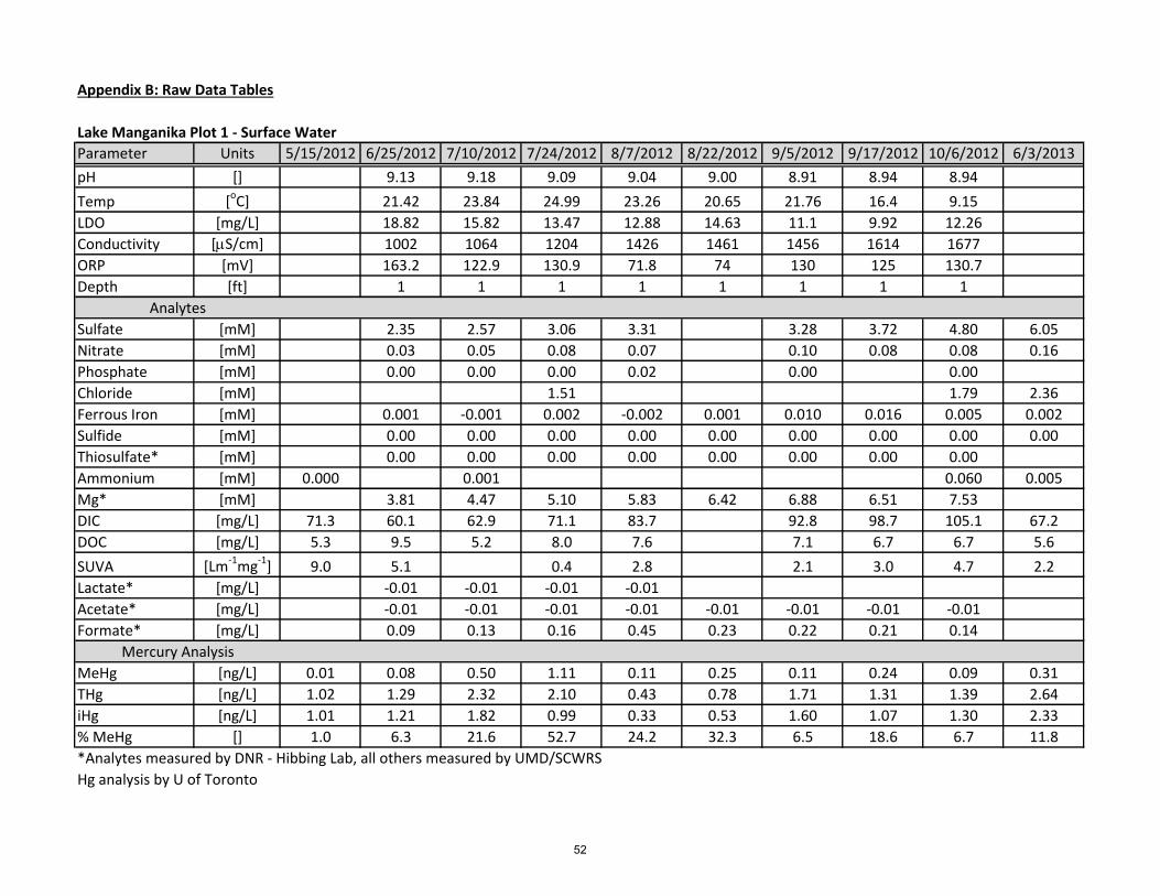
Appendix B: Raw Data Tables

Lake Manganika Plot 1 - Surface Water

Parameter Units 5/15/2012 6/25/2012 7/10/2012 7/24/2012 8/7/2012 8/22/2012 9/5/2012 9/17/2012 10/6/2012 6/3/2013

pH [] 9.13 9.18 9.09 9.04 9.00 8.91 8.94 8.94

Temp [oC] 21.42 23.84 24.99 23.26 20.65 21.76 16.4 9.15

LDO [mg/L] 18.82 15.82 13.47 12.88 14.63 11.1 9.92 12.26

Conductivity [mS/cm] 1002 1064 1204 1426 1461 1456 1614 1677

ORP [mV] 163.2 122.9 130.9 71.8 74 130 125 130.7

Depth [ft] 1 1 1 1 1 1 1 1

Sulfate [mM] 2.35 2.57 3.06 3.31 3.28 3.72 4.80 6.05

Nitrate [mM] 0.03 0.05 0.08 0.07 0.10 0.08 0.08 0.16

Phosphate [mM] 0.00 0.00 0.00 0.02 0.00 0.00

Chloride [mM] 1.51 1.79 2.36

Ferrous Iron [mM] 0.001 -0.001 0.002 -0.002 0.001 0.010 0.016 0.005 0.002

Sulfide [mM] 0.00 0.00 0.00 0.00 0.00 0.00 0.00 0.00 0.00

Thiosulfate* [mM] 0.00 0.00 0.00 0.00 0.00 0.00 0.00 0.00

Ammonium [mM] 0.000 0.001 0.060 0.005

Mg* [mM] 3.81 4.47 5.10 5.83 6.42 6.88 6.51 7.53

DIC [mg/L] 71.3 60.1 62.9 71.1 83.7 92.8 98.7 105.1 67.2

DOC [mg/L] 5.3 9.5 5.2 8.0 7.6 7.1 6.7 6.7 5.6

SUVA [Lm-1mg-1] 9.0 5.1 0.4 2.8 2.1 3.0 4.7 2.2

Lactate* [mg/L] -0.01 -0.01 -0.01 -0.01

Acetate* [mg/L] -0.01 -0.01 -0.01 -0.01 -0.01 -0.01 -0.01 -0.01

Formate* [mg/L] 0.09 0.13 0.16 0.45 0.23 0.22 0.21 0.14

MeHg [ng/L] 0.01 0.08 0.50 1.11 0.11 0.25 0.11 0.24 0.09 0.31

THg [ng/L] 1.02 1.29 2.32 2.10 0.43 0.78 1.71 1.31 1.39 2.64

iHg [ng/L] 1.01 1.21 1.82 0.99 0.33 0.53 1.60 1.07 1.30 2.33

% MeHg [] 1.0 6.3 21.6 52.7 24.2 32.3 6.5 18.6 6.7 11.8

*Analytes measured by DNR - Hibbing Lab, all others measured by UMD/SCWRS

Hg analysis by U of Toronto

Analytes

Mercury Analysis

52

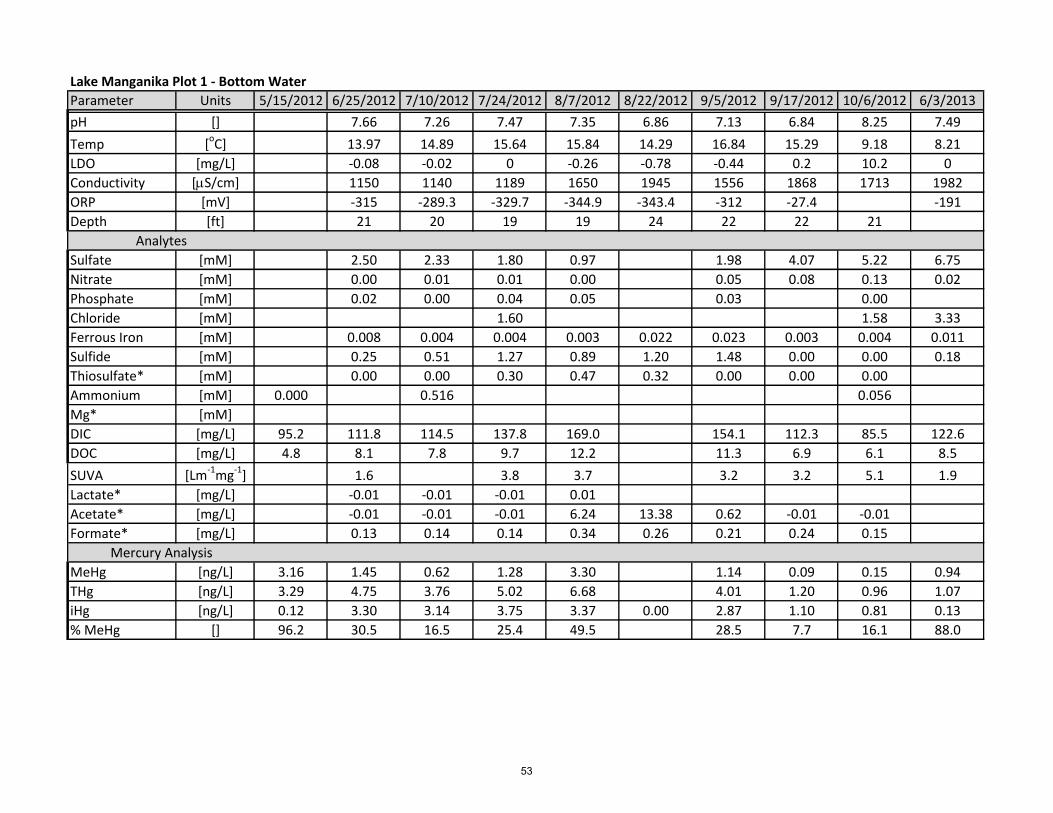
Lake Manganika Plot 1 - Bottom Water

Parameter Units 5/15/2012 6/25/2012 7/10/2012 7/24/2012 8/7/2012 8/22/2012 9/5/2012 9/17/2012 10/6/2012 6/3/2013

pH [] 7.66 7.26 7.47 7.35 6.86 7.13 6.84 8.25 7.49

Temp [oC] 13.97 14.89 15.64 15.84 14.29 16.84 15.29 9.18 8.21

LDO [mg/L] -0.08 -0.02 0 -0.26 -0.78 -0.44 0.2 10.2 0

Conductivity [mS/cm] 1150 1140 1189 1650 1945 1556 1868 1713 1982

ORP [mV] -315 -289.3 -329.7 -344.9 -343.4 -312 -27.4 -191

Depth [ft] 21 20 19 19 24 22 22 21

Sulfate [mM] 2.50 2.33 1.80 0.97 1.98 4.07 5.22 6.75

Nitrate [mM] 0.00 0.01 0.01 0.00 0.05 0.08 0.13 0.02

Phosphate [mM] 0.02 0.00 0.04 0.05 0.03 0.00

Chloride [mM] 1.60 1.58 3.33

Ferrous Iron [mM] 0.008 0.004 0.004 0.003 0.022 0.023 0.003 0.004 0.011

Sulfide [mM] 0.25 0.51 1.27 0.89 1.20 1.48 0.00 0.00 0.18

Thiosulfate* [mM] 0.00 0.00 0.30 0.47 0.32 0.00 0.00 0.00

Ammonium [mM] 0.000 0.516 0.056

Mg* [mM]

DIC [mg/L] 95.2 111.8 114.5 137.8 169.0 154.1 112.3 85.5 122.6

DOC [mg/L] 4.8 8.1 7.8 9.7 12.2 11.3 6.9 6.1 8.5

SUVA [Lm-1

mg-1

] 1.6 3.8 3.7 3.2 3.2 5.1 1.9

Lactate* [mg/L] -0.01 -0.01 -0.01 0.01

Acetate* [mg/L] -0.01 -0.01 -0.01 6.24 13.38 0.62 -0.01 -0.01

Formate* [mg/L] 0.13 0.14 0.14 0.34 0.26 0.21 0.24 0.15

MeHg [ng/L] 3.16 1.45 0.62 1.28 3.30 1.14 0.09 0.15 0.94

THg [ng/L] 3.29 4.75 3.76 5.02 6.68 4.01 1.20 0.96 1.07

iHg [ng/L] 0.12 3.30 3.14 3.75 3.37 0.00 2.87 1.10 0.81 0.13

% MeHg [] 96.2 30.5 16.5 25.4 49.5 28.5 7.7 16.1 88.0

Analytes

Mercury Analysis

53

Lake Manganika - Plot 1 Profiles (1 of 3)

Parameter Units

Depth [ft] 1 4 6 7 10 12 13 16 19 21

pH [] 9.13 9.04 8.54 8.35 8.36 7.98 7.76 7.66

Temp [oC] 21.42 20.35 18.94 18.06 17.01 15.21 14.34 13.97

LDO [mg/L] 18.82 17.14 5.48 1.94 0.08 0.04 -0.04 -0.08

Conductivity [mS/cm] 1002 981 1017 1068 1191 1184 1158 1150

ORP [mV] 163.2 157.7 160.8 147.4 -66 -270 -288 -315

Depth [ft]

Sulfate [mM] 2.35 2.70 2.71 3.40 3.08 2.50

Nitrate [mM] 0.03 0.17 0.09 0.00

Phosphate [mM] 0.00 0.00 0.00 0.00 0.02

Chloride [mM]

Ferrous Iron [mM] 0.001 0.001 0.000 0.011 0.008

Sulfide [mM] 0.00 0.00 0.00 0.00 0.22 0.25

Thiosulfate* [mM]

Ammonium [mM]

Mg* [mM]

DIC [mg/L] 60.1 68.8 73.8 91.1 103.5 111.8

DOC [mg/L] 9.5 9.6 9.2 8.5 7.3 8.1

SUVA [Lm-1

mg-1

] 5.1 1.3 2.1 1.0 4.5 1.6

Lactate* [mg/L]

Acetate* [mg/L]

Formate* [mg/L]

MeHg [ng/L] 0.08 0.08 0.21 0.74 1.01 1.45

THg [ng/L] 1.29 1.90 2.20 2.68 5.08 4.75

iHg [ng/L] 1.21 1.82 1.99 1.94 4.07 3.30

%MeHg [] 6.3 4.1 9.5 27.6 19.8 30.5

Analytes

Mercury Analysis

6/25/2012

54

Lake Manganika - Plot 1 Profiles (2 of 3)

Parameter Units

Depth [ft] 1 4 7 10 13 14 16 19 1 4 7 10 13 16 19 24

pH [] 9.09 9 8.9 8.63 7.77 7.53 7.47 9 8.97 8.92 8.72 8.47 7.81 7.41 6.86

Temp [oC] 24.99 24.86 24.67 22.21 17.89 16.14 15.64 20.65 20.22 19.82 19.45 18.97 17.9 16.63 14.29

LDO [mg/L] 13.47 8.25 3.99 0.04 14.63 12.97 10.28 0.34 0.04 -0.09 -0.47 -0.78

Conductivity [mS/cm] 1204 1217 1245 1336 1232 1194 1189 1461 1464 1492 1527 1631 1668 1686 1945

ORP [mV] 130.9 124.7 118.3 -160 -303 -321 -330 74 68.9 65.4 62.6 -310 -334 -350 -343

Depth [ft]

Sulfate [mM] 3.06 3.14 3.34 3.31 2.20 1.80

Nitrate [mM] 0.08 0.08 0.11 0.00 0.01 0.01

Phosphate [mM] 0.00 0.00 0.00 0.00 0.02 0.04

Chloride [mM] 1.51 1.52 1.50 1.43 1.54 1.60

Ferrous Iron [mM] 0.002 -0.002 -0.002 0.004 0.001 0.002 0.002 0.005 0.017 0.011 0.022

Sulfide [mM] 0.00 0.00 0.00 0.09 0.57 1.27 0.00 0.00 0.00 0.00 0.12 0.80 1.20

Thiosulfate* [mM]

Ammonium [mM]

Mg* [mM]

DIC [mg/L] 71.1 79.5 82.2 106.7 127.5 137.8

DOC [mg/L] 8.0 8.5 7.6 10.6 11.0 9.7

SUVA [Lm-1

mg-1

] 0.4 2.6 5.6 2.4 2.9 3.8

Lactate* [mg/L]

Acetate* [mg/L]

Formate* [mg/L]

MeHg [ng/L] 1.11 0.24 0.05 1.78 0.64 1.28 0.25 0.44 0.07 0.45 1.28

THg [ng/L] 2.10 1.18 1.04 4.92 3.89 5.02 0.78 0.61 0.50 0.93 4.20

iHg [ng/L] 0.99 0.94 0.99 3.15 3.25 3.75 0.53 0.18 0.43 0.49 2.92

%MeHg [] 52.7 20.5 5.1 36.1 16.5 25.4 32.3 71.4 13.9 48.0 30.4

Analytes

Mercury Analysis

7/24/2012 8/21/2012

55

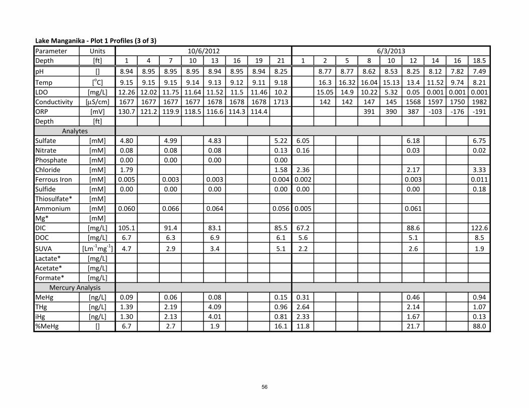
Lake Manganika - Plot 1 Profiles (3 of 3)

Parameter Units

Depth [ft] 1 4 7 10 13 16 19 21 1 2 5 8 10 12 14 16 18.5

pH [] 8.94 8.95 8.95 8.95 8.94 8.95 8.94 8.25 8.77 8.77 8.62 8.53 8.25 8.12 7.82 7.49

Temp [oC] 9.15 9.15 9.15 9.14 9.13 9.12 9.11 9.18 16.3 16.32 16.04 15.13 13.4 11.52 9.74 8.21

LDO [mg/L] 12.26 12.02 11.75 11.64 11.52 11.5 11.46 10.2 15.05 14.9 10.22 5.32 0.05 0.001 0.001 0.001

Conductivity [mS/cm] 1677 1677 1677 1677 1678 1678 1678 1713 142 142 147 145 1568 1597 1750 1982

ORP [mV] 130.7 121.2 119.9 118.5 116.6 114.3 114.4 391 390 387 -103 -176 -191

Depth [ft]

Sulfate [mM] 4.80 4.99 4.83 5.22 6.05 6.18 6.75

Nitrate [mM] 0.08 0.08 0.08 0.13 0.16 0.03 0.02

Phosphate [mM] 0.00 0.00 0.00 0.00

Chloride [mM] 1.79 1.58 2.36 2.17 3.33

Ferrous Iron [mM] 0.005 0.003 0.003 0.004 0.002 0.003 0.011

Sulfide [mM] 0.00 0.00 0.00 0.00 0.00 0.00 0.18

Thiosulfate* [mM]

Ammonium [mM] 0.060 0.066 0.064 0.056 0.005 0.061

Mg* [mM]

DIC [mg/L] 105.1 91.4 83.1 85.5 67.2 88.6 122.6

DOC [mg/L] 6.7 6.3 6.9 6.1 5.6 5.1 8.5

SUVA [Lm-1

mg-1

] 4.7 2.9 3.4 5.1 2.2 2.6 1.9

Lactate* [mg/L]

Acetate* [mg/L]

Formate* [mg/L]

MeHg [ng/L] 0.09 0.06 0.08 0.15 0.31 0.46 0.94

THg [ng/L] 1.39 2.19 4.09 0.96 2.64 2.14 1.07

iHg [ng/L] 1.30 2.13 4.01 0.81 2.33 1.67 0.13

%MeHg [] 6.7 2.7 1.9 16.1 11.8 21.7 88.0

Analytes

Mercury Analysis

6/3/201310/6/2012

56

Lake Manganika Plot 2 - Surface Water

Parameter Units 5/15/2012 6/25/2012 7/10/2012 7/24/2012 8/7/2012 8/22/2012 9/5/2012 9/17/2012 10/6/2012 6/3/2013

pH [] 9.29 9.25 9.06 9.01 8.89 8.96 8.98

Temp [oC] 25.5 24.5 25.96 23.42 20.64 16.47 9.16

LDO [mg/L] 18.97 18.42 14.2 11.5 9.41 10.71 12.25

Conductivity [mS/cm] 1060 1064 1213 1438 1486 1613 1674

ORP [mV] 14.9 17.2 -21 7.3 21.5

Depth [ft]

Sulfate [mM] 2.96 4.71

Nitrate [mM] 0.08 0.10

Phosphate [mM] 0.00

Chloride [mM] 1.54 1.68

Ferrous Iron [mM] 0.002 0.004

Sulfide [mM] 0.00 0.00 0.00

Thiosulfate* [mM]

Ammonium [mM] 0.000 0.062

Mg* [mM]

DIC [mg/L] 85.6 70.6 78.4

DOC [mg/L] 4.8 9.5 6.5

SUVA [Lm-1

mg-1

] 9.9 3.1 4.8

Lactate* [mg/L]

Acetate* [mg/L]

Formate* [mg/L]

MeHg [ng/L] 0.06 0.29 0.01 0.19 0.09 0.16

THg [ng/L] 2.12 1.46 0.57 2.03 0.78 1.66

iHg [ng/L] 2.06 1.17 0.56 1.84 0.69 1.50

% MeHg [] 2.7 20.0 1.8 9.6 11.9 9.4

Analytes

Mercury Analysis

57

Lake Manganika Plot 2 - Bottom Water

Parameter Units 5/15/2012 6/25/2012 7/10/2012 7/24/2012 8/7/2012 8/22/2012 9/5/2012 9/17/2012 10/6/2012 6/3/2013

pH [] 8.59 8.57 7.47 7.70 8.75 8.95 8.98 8.55

Temp [oC] 18.9 21.16 22.28 21.7 19.53 16.47 9.11 15.48

LDO [mg/L] 9.97 0.32 -0.17 0.08 1.43 10.42 11.81 4.85

Conductivity [mS/cm] 1026 1118 1306 1489 1503 1615 1675 1454

ORP [mV] 9 -179 -361.4 -329 -123 11.9 31.4

Depth [ft] 8 9 9 9 9 7 7

Sulfate [mM] 3.29 4.87 3.00

Nitrate [mM] 0.10 0.08 0.12

Phosphate [mM] 0.00

Chloride [mM] 1.52 2.36

Ferrous Iron [mM] -0.001 -0.002 0.001 0.005 0.002

Sulfide [mM] 0.00 0.00 0.00 0.00 0.00

Thiosulfate* [mM]

Ammonium [mM] 0.092 0.065 0.002

Mg* [mM]

DIC [mg/L] 77.2 89.2 78.2 70.7

DOC [mg/L] 8.0 8.3 6.5 5.8

SUVA [Lm-1

mg-1

] 3.4 3.1 2.3

Lactate* [mg/L]

Acetate* [mg/L]

Formate* [mg/L]

MeHg [ng/L] 0.18 0.10 0.14 0.09 0.20

THg [ng/L] 1.55 0.96 0.74 4.56 4.07

iHg [ng/L] 1.37 0.86 0.61 4.47 3.87

% MeHg [] 11.5 10.6 18.3 2.1 5.0

Analytes

Mercury Analysis

58

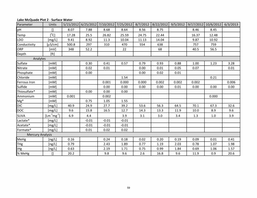
Lake McQuade Plot 2 - Surface Water

Parameter Units 5/15/2012 6/25/2012 7/10/2012 7/25/2012 8/7/2012 8/22/2012 9/5/2012 9/17/2012 10/6/2012 6/3/2013

pH [] 8.07 7.88 8.68 8.64 8.56 8.75 8.46 8.45

Temp [oC] 17.28 25.5 26.82 25.59 24.75 22.44 16.37 12.48

LDO [mg/L] 9.41 8.92 11.3 10.04 11.13 14.04 9.87 10.92

Conductivity [mS/cm] 500.8 297 310 470 554 638 757 759

ORP [mV] 348 52.2 22 68 40.5 56.5

Depth [ft]

Sulfate [mM] 0.30 0.41 0.57 0.79 0.93 0.88 1.00 1.23 3.28

Nitrate [mM] 0.02 0.01 0.00 0.01 0.05 0.07 0.01

Phosphate [mM] 0.00 0.00 0.02 0.01

Chloride [mM] 1.54 0.21

Ferrous Iron [mM] 0.001 0.000 0.000 0.002 0.002 0.002 0.006

Sulfide [mM] 0.00 0.00 0.00 0.00 0.01 0.00 0.00 0.00

Thiosulfate* [mM] 0.00 0.00 0.00

Ammonium [mM] 0.001 0.002 0.000

Mg* [mM] 0.75 1.05 1.55

DIC [mg/L] 40.9 24.9 27.7 39.2 53.6 56.3 64.5 70.1 67.3 32.6

DOC [mg/L] 9.6 15.8 16.5 12.7 14.3 13.3 11.9 10.0 8.9 9.6

SUVA [Lm-1

mg-1

] 6.9 4.4 3.9 3.1 3.0 3.4 1.3 1.0 3.9

Lactate* [mg/L] -0.01 -0.01 -0.01

Acetate* [mg/L] -0.01 -0.01 -0.01

Formate* [mg/L] 0.01 0.02 0.02

MeHg [ng/L] 0.16 0.24 0.18 0.02 0.20 0.19 0.09 0.01 0.41

THg [ng/L] 0.79 2.43 1.89 0.77 1.19 2.03 0.78 1.07 1.98

iHg [ng/L] 0.63 2.19 1.71 0.75 0.99 1.84 0.69 1.06 1.57

% MeHg [] 20.2 9.8 9.6 2.6 16.8 9.6 11.9 0.9 20.6

Analytes

Mercury Analysis

59

Lake McQuade Plot 2 - Bottom Water

Parameter Units 5/15/2012 6/25/2012 7/10/2012 7/25/2012 8/7/2012 8/22/2012 9/5/2012 9/17/2012 10/6/2012 6/3/2013

pH [] 7.98 6.92 7.32 7.26 7.76 7.99 8.44 8.43 7.40

Temp [oC] 15.3 16.55 17.18 18.99 21 18.02 16.31 12.5 13.86

LDO [mg/L] 7.17 0.27 0.04 0.02 0.6 3.59 8.91 10.78 6.19

Conductivity [mS/cm] 499.4 187 236 427 663 833 760 759 461

ORP [mV] 333 71.2 -70.5 -120 -60 -70.4 41.2 67.1

Depth [ft] 9 9 8.5 9 10 10 9

Sulfate [mM] 0.19 0.28 0.57 0.95 1.47 1.24

Nitrate [mM] 0.01 0.00 0.01 0.03 0.06 0.00

Phosphate [mM] 0.01 0.01 0.01

Chloride [mM] 1.49 0.22

Ferrous Iron [mM] 0.014 0.006 -0.002 0.004

Sulfide [mM] 0.00 0.00 0.00 0.00 0.00 0.00

Thiosulfate* [mM] 0.00 0.00 0.00

Ammonium [mM] 0.036 0.002

Mg* [mM] 0.55 1.64 1.64

DIC [mg/L] 20.4 31.4 47.6 63.9 72.9 66.2

DOC [mg/L] 17.7 18.1 13.4 10.0 6.7 8.9

SUVA [Lm-1

mg-1

] 4.6 4.3 3.7 3.6 1.0

Lactate* [mg/L] -0.01 -0.01 -0.01

Acetate* [mg/L] -0.01 -0.01 -0.01

Formate* [mg/L] -0.01 0.01 0.02

MeHg [ng/L] 1.32 0.39 0.09 0.09 0.07 0.21

THg [ng/L] 3.45 1.74 1.03 0.77 0.99 4.23

iHg [ng/L] 2.13 1.35 0.95 0.68 0.92 4.02

% MeHg [] 38.3 22.3 8.2 11.4 7.1 5.0

Analytes

Mercury Analysis

60

Lake McQuade Plot 3 - Surface Water

Parameter Units 5/15/2012 6/25/2012 7/10/2012 7/25/2012 8/7/2012 8/22/2012 9/5/2012 9/17/2012 10/6/2012 6/3/2013

pH [] 7.80 8.56 8.47 8.35 8.45 8.37 8.44 8.29

Temp [oC] 24.8 27.24 25.11 24.27 20.77 20.73 16.77 13.24

LDO [mg/L] 8.21 10.5 8.26 9.81 9.8 5.7 9.92 10.7

Conductivity [mS/cm] 300 276 441 539 623 648 732 737

ORP [mV] 72.2 32.9 117 139.6 115 43.5 132.9

Depth [ft]

Sulfate [mM] 0.32 0.41 0.53 0.77 0.89 0.88 0.95 1.21 3.27

Nitrate [mM] 0.01 0.01 0.01 0.01 0.00 0.05 0.05 0.00 0.01

Phosphate [mM] 0.00

Chloride [mM] 0.21 0.31

Ferrous Iron [mM] 0.002 0.001 0.000 -0.002 0.002 0.001 0.002 0.003

Sulfide [mM] 0.00 0.00 0.00 0.00 0.00 0.00 0.00 0.00 0.00

Thiosulfate* [mM]

Ammonium [mM] 0.001 0.002 0.001

Mg* [mM] 0.77 0.91 0.91 1.89 2.15 2.42 2.22 2.58

DIC [mg/L] 25.7 25.8 36.5 47.6 56.9 62.6 66.5 67.8 34.2

DOC [mg/L] 16.9 16.6 13.3 12.1 12.2 12.3 10.4 10.3 8.3

SUVA [Lm-1

mg-1

] 4.1 4.0 3.9 3.9 3.3 1.5 2.8 3.5

Lactate* [mg/L] -0.01 -0.01 -0.01 -0.01

Acetate* [mg/L] -0.01 -0.01 -0.01 -0.01 -0.01 -0.01 -0.01 -0.01

Formate* [mg/L] 0.01 0.01 0.02 0.07 0.04 0.04 0.04 0.01

MeHg [ng/L] 0.21 0.43 0.13 0.10 0.08 0.06 0.05 0.11 0.14

THg [ng/L] 2.78 2.87 1.52 0.84 0.67 1.24 1.20 0.91 2.74

iHg [ng/L] 2.57 2.45 1.38 0.74 0.59 1.18 1.15 0.81 2.60

% MeHg [] 7.6 14.8 8.8 12.0 12.3 5.0 4.4 11.5 5.1

Analytes

Mercury Analysis

61

Lake McQuade Plot 3 - Bottom Water

Parameter Units 5/15/2012 6/25/2012 7/10/2012 7/25/2012 8/7/2012 8/22/2012 9/5/2012 9/17/2012 10/6/2012 6/3/2013

pH [] 7.05 6.84 6.76 6.78 7.30 7.23 8.37 8.29

Temp [oC] 13.81 13.81 14.43 15.02 16.37 16.66 16.67 13.19

LDO [mg/L] 0.05 0.01 0.06 0.01 0.04 8.49 10.19

Conductivity [mS/cm] 256 207 302 387 628 594 734 738

ORP [mV] -183.7 -173 -221 -205.6 -241.7 -277

Depth [ft] 15 15 14 15.5 15 15 15

Sulfate [mM] 0.16 0.16 0.06 0.04 0.72 0.67 0.92 1.20 3.28

Nitrate [mM] 0.00 0.01 0.00 0.00 0.05 0.04 0.01

Phosphate [mM] 0.01 0.00 0.03 0.04 0.02 0.02 0.00 0.00

Chloride [mM] 0.21 0.29

Ferrous Iron [mM] 0.008 0.009 0.024 0.025 0.013 0.008 0.001 0.004

Sulfide [mM] 0.01 0.00 0.00 0.00 0.00 0.02 0.00 0.00 0.00

Thiosulfate* [mM]

Ammonium [mM] 0.002 0.006

Mg* [mM] 0.78 0.79 0.85 0.97 2.01 2.25 2.23 2.58

DIC [mg/L] 31.5 31.9 35.7 45.0 62.0 73.1 65.4 70.1 35.4

DOC [mg/L] 16.2 17.0 18.6 21.7 12.8 13.1 10.3 9.4 7.6

SUVA [Lm-1

mg-1

] 4.5 5.1 4.7 4.3 2.3 1.4 3.1 3.5

Lactate* [mg/L] -0.01 -0.01 0.01 0.01

Acetate* [mg/L] -0.01 -0.01 0.01 0.01 -0.01 -0.01 -0.01 -0.01

Formate* [mg/L] -0.01 -0.01 0.01 0.02 0.03 0.07 0.04 -0.01

MeHg [ng/L] 1.29 2.46 1.52 6.50 1.99 0.68 0.08 0.12 0.21

THg [ng/L] 2.82 4.63 3.29 8.08 2.68 2.39 1.48 0.89 2.58

iHg [ng/L] 1.53 2.17 1.77 1.58 0.70 1.71 1.41 0.76 2.37

% MeHg [] 45.7 53.2 46.1 80.4 74.0 28.6 5.1 14.0 8.3

Analytes

Mercury Analysis

62

Lake McQuade - Plot 3 Profiles (1 of 2)

Parameter Units

Depth [ft] 1 4 5 7 9 10 11 13 15 1 4 7 9 12 14

pH [] 7.8 7.4 7.03 7.01 7.14 7.05 8.47 6.76

Temp [oC] 24.8 20.29 17.26 16.41 15.36 13.81 25.11 14.43

LDO [mg/L] 8.21 5.95 1.33 0.25 0.11 0.05 8.26

Conductivity [mS/cm] 300 266 199 213 268 256 441 302

ORP [mV] 72.2 84.5 89.9 83.7 -102.6 -183.7 117 -221

Depth [ft]

Sulfate [mM] 0.32 0.26 0.23 0.25 0.30 0.16 0.53 0.53 0.55 0.38 0.17 0.06

Nitrate [mM] 0.01 0.02 0.01 0.01 0.00 0.01 0.00 0.00 0.01 0.01 0.01

Phosphate [mM] 0.00 0.01 0.02 0.03

Chloride [mM]

Ferrous Iron [mM] 0.002 0.004 0.006 0.006 0.006 0.008 0.000 0.000 0.001 0.003 0.022 0.024

Sulfide [mM] 0.000 0.002 0.002 0.001 0.002 0.006 0.000 0.000 0.000 0.001 0.001 0.000

Thiosulfate* [mM]

Ammonium [mM]

Mg* [mM]

DIC [mg/L] 25.7 22.6 21.9 24.2 30.5 31.5 36.5 38.6 41.6 35.7 33.2 35.7

DOC [mg/L] 16.9 18.5 18.4 17.6 16.1 16.2 13.3 11.6 13.4 15.3 16.9 18.6

SUVA [Lm-1

mg-1

] 4.1 4.3 4.6 4.4 4.6 4.5 4.0 4.7 4.1 4.3 5.0 5.1

Lactate* [mg/L]

Acetate* [mg/L]

Formate* [mg/L]

MeHg [ng/L] 0.21 0.38 0.64 0.92 2.11 1.29 0.13 0.20 0.52 0.63 0.95 1.52

THg [ng/L] 2.78 4.07 4.65 4.85 4.11 2.82 1.52 1.93 1.67 1.63 2.13 3.29

iHg [ng/L] 2.57 3.69 4.01 3.93 2.00 1.53 1.38 1.72 1.15 1.00 1.18 1.77

%MeHg [] 7.6 9.3 13.8 19.1 51.4 45.7 8.8 10.6 31.4 38.4 44.8 46.1

Mercury Analysis

6/25/2012 7/25/2012

Analytes

63

Lake McQuade - Plot 3 Profiles (2 of 2)

Parameter Units

Depth [ft] 1 4 7 10 12 13 15 1 5 10 14 15

pH [] 8.45 8.39 7.94 7.97 7.52 7.3 8.29 8.32 8.33 8.35 8.29

Temp [oC] 20.77 20.25 19.55 19.12 17.67 16.37 13.24 13.25 13.25 13.24 13.19

LDO [mg/L] 9.8 9.17 3.2 2.89 0.11 0.01 10.7 10.66 10.72 10.65 10.19

Conductivity [mS/cm] 623 634 666 706 671 628 737 737 737 738 738

ORP [mV] 139.6 129.1 139 136.1 -200.8 -241.7 132.9 133.6 131.6

Depth [ft]

Sulfate [mM] 0.89 0.93 1.08 0.98 0.72 1.21 1.16 1.21 1.20

Nitrate [mM] 0.00 0.01 0.03 0.00 0.00 0.00 0.01 0.00

Phosphate [mM] 0.01 0.02 0.00 0.00 0.00

Chloride [mM] 0.24 0.21 0.21 0.21 0.21

Ferrous Iron [mM] 0.002 0.002 0.001 0.001 0.013 0.004 0.003

Sulfide [mM] 0.001 0.002 0.002 0.001 0.004 0.000 0.001 0.001 0.001

Thiosulfate* [mM]

Ammonium [mM] 0.002 0.003 0.003 0.002

Mg* [mM]

DIC [mg/L] 56.9 61.1 64.1 64.8 62.0 67.8 69.7 67.7 70.1

DOC [mg/L] 12.2 11.1 9.9 11.4 12.8 10.3 9.8 10.1 9.4

SUVA [Lm-1

mg-1

] 3.9 3.6 3.6 4.0 4.3 2.8 3.1 2.9 3.1

Lactate* [mg/L]

Acetate* [mg/L]

Formate* [mg/L]

MeHg [ng/L] 0.08 0.13 0.34 0.38 1.99 0.11 0.05 0.11 0.12

THg [ng/L] 0.67 0.90 0.74 0.71 2.68 0.91 0.94 1.22 0.89

iHg [ng/L] 0.59 0.77 0.40 0.33 0.70 0.81 0.89 1.11 0.76

%MeHg [] 12.3 14.9 46.0 53.2 74.0 11.5 5.6 9.3 14.0

8/21/2012 10/6/2012

Analytes

Mercury Analysis

64