Embed Size (px)
Citation preview

MEDICAL STUDENT DEMOGRAPHICS AND ATTITUDES AS PREDICTORS FOR FUTURE RURAL PRACTICE
by
Jordan Smith
B.A. Mathematical Sciences, Binghamton University, State University of New York, 2011
Submitted to the Graduate Faculty of
the Graduate School of Public Health in partial fulfillment
of the requirements for the degree of
Master of Science
University of Pittsburgh
2013

UNIVERSITY OF PITTSBURGH
Graduate School of Public Health
This thesis was presented
by
Jordan Smith
It was defended on
April 9th, 2013
and approved by
Thesis Director: Jeanine Buchanich, PhD, Research Assistant Professor, Biostatistics, Graduate School of Public Health, University of Pittsburgh
Sally Morton, PhD, Professor and Chair, Biostatistics, Graduate School of Public Health,
University of Pittsburgh
Christopher P. Morley, PhD, Associate Professor, Department of Family Medicine, Department of Public Health & Preventive Medicine, and Department of Psychiatry &
Behavioral Sciences, SUNY Upstate Medical University
Evelyn Talbott, PhD, Professor, Epidemiology, Graduate School of Public Health, University of Pittsburgh
ii

Copyright © by Jordan Smith
2013
iii

ABSTRACT
Introduction: American medical schools are struggling to identify students who would consider a career
in rural health. The deficiency of healthcare professionals in rural locations is widespread across the U.S.,
and it is projected that the shortage will worsen at the current rate which students are going into rural
practice. The lack of easy access to health care for rural residents is of public health significance. The
purpose of this study was to examine changes in medical student interests and attitudes relating to rural
location and its needed specialists medical students over time, as well as identifying which demographic
information, interests, and attitudes that significantly predict interest in future rural practice.
Methods: The study participants were first and second year medical students at an allopathic medical
school in the U.S. who were enrolled in an introductory clinical skills course. We sought to identify
differences in survey responses between first-year and second-year medical students at the beginning and
end of Academic Year 2010 on items relating to work setting, motivations for pursuing a medical career
or specialty, interest in underserved populations, and attitudes toward primary care. Principle components
analysis was used to extract linear composite variables (LCV) from responses to each group of questions;
ordinary least squares (OLS) regression was then used to identify potential demographic and attitudinal
predictors for future rural practice.
Results: Interest in rural health and its needed specialties significantly declined over the pre-clinical
years. Rural background, interest in generalist specialties, and idealistic motivations were consistent
Jeanine Buchanich, PhD
MEDICAL STUDENT DEMOGRAPHICS AND ATTITUDES AS PREDICTORS FOR FUTURE RURAL PRACTICE
Jordan Smith, M.S.
University of Pittsburgh, 2013
iv

positive predictors for future rural practice. Marital status and being female were also found to positively
predict interest in rural practice, while being in the second year of medical school was found to decrease
interest in future rural practice. Importance of money, prestige, and lifestyle in choice of career was found
to negatively impact the likelihood of rural practice.
Conclusion: The results support previous research suggesting rural background, interest in generalist
specialties, and idealistic motivations are positive predictors for future rural practice. Female gender and
white race were inconsistent in their significance as predictors, and should be studied further.
v
TABLE OF CONTENTS
PREFACE .................................................................................................................................. XII
1.0 INTRODUCTION ........................................................................................................ 1
1.1 RURAL HEALTHCARE PROFESSIONAL DEFICIENCIES ...................... 2
1.2 MEDICAL SCHOOL PRODUCTION OF RURAL PRACTITIONERS ..... 3
1.2.1 Osteopathic and Allopathic Medical Schools ............................................. 5
1.3 ESTABLISHED PREDICTORS OF FUTURE RURAL PRACTICE ........... 5
2.0 METHODS ................................................................................................................... 9
2.1.1 Data methods ............................................................................................... 11
2.1.2 Survey Development ................................................................................... 13
2.1.3 Survey Implementation .............................................................................. 14
2.2 METHODS OF COMPARISON...................................................................... 15
2.2.1 Mann-Whitney U Test ................................................................................ 15
2.3 DATA REDUCTION......................................................................................... 16
2.3.1 Principal Component Analysis (PCA) ...................................................... 16
2.3.1.1 Student’s T-Test .................................................................................. 18
2.4 SCALE CREATION ......................................................................................... 19
2.4.1 Cronbach’s α ............................................................................................... 19
2.5 METHODS FOR FINDING PREDICTORS OF RURAL HEALTH .......... 20
vi

2.5.1 Ordinary Least Squares (OLS) Regression .............................................. 20
3.0 APPLICATION OF METHODOLOGY ................................................................. 23
3.1 ANALYSIS PLAN ............................................................................................. 23
3.1.1 Comparisons of Original Survey Responses............................................. 23
3.1.1.1 Tests of Normality (Shapiro-Wilk) .................................................... 24
3.1.1.2 Mann- Whitney U Test ....................................................................... 25
3.1.2 Data Reduction via Principal Components Analysis ............................... 25
3.1.2.1 Two Independent Sample Student’s T-test ....................................... 26
3.1.3 Finding significant predictors for future rural practice ......................... 27
3.1.3.1 Finding significant demographic predictors for future rural
practice. ............................................................................................................... 27
3.1.3.2 Finding significant demographic and attitude predictors for future
rural practice ...................................................................................................... 28
3.1.4 Creation of a new rural dependent variable............................................. 28
3.1.4.1 Creating the scale using Cronbach’s α .............................................. 28
3.1.4.2 Turning the scale into a linear composite variable via Principal
Components Analysis ........................................................................................ 29
3.1.4.3 Finding significant demographic predictors for the new rural
dependent variable............................................................................................. 29
3.1.4.4 Finding significant demographic and attitude predictors for the
new rural dependent variable ........................................................................... 30
3.1.5 Analyzing final models with regression diagnostics ................................ 30
4.0 RESULTS ................................................................................................................... 32
vii
4.1.1 Comparability between MS1 and MS2, as well as to national statistics 32
4.1.2 Comparisons between time points on original survey responses ........... 33
4.1.3 Principal Components Analysis ................................................................. 36
4.1.4 Student t-test comparisons between time points on extracted principal
components ................................................................................................................. 38
4.1.5 Ordinary Least Squares Regression on “Rural Setting” linear composite
variable.. ...................................................................................................................... 39
4.1.5.1 Using demographic predictors ........................................................... 39
4.1.5.2 Using extracted principal components .............................................. 40
4.1.5.3 Using demographic information and linear composite variables ... 41
4.1.5.4 Final models, which include rural upbringing as a mandatory
predictor ............................................................................................................. 43
4.2 ANALYSIS OF NEW MANUALLY CREATED RURAL COMPOSITE
DEPENDENT VARIABLE ............................................................................................... 44
4.2.1 Ordinary Least Squares Regression on demographic predictors .......... 44
4.2.2 Final models, including rural upbringing as a mandatory predictor .... 45
4.3 FINAL MODEL REGRESSION DIAGNOSTICS ........................................ 47
5.0 DISCUSSION ............................................................................................................. 50
6.0 CONCLUSION ........................................................................................................... 59
APPENDIX A. SURVEY INSTRUMENT ............................................................................... 61
APPENDIX B. INSTITUTIONAL REVIEW BOARD EXEMPTION ................................. 68
APPENDIX C. MANN-WHITNEY U BEGIN MS1 – BEGIN MS2 ...................................... 70
APPENDIX D. MANN-WHITNEY U END MS1 – END MS2 ............................................... 72
viii

APPENDIX E. MANN-WHITNEY U GENDER COMPARISON ........................................ 74
APPENDIX F. IMPORTANT PRINCIPAL COMPONENTS AND T-TESTS FOR BEGIN
MS YEAR .................................................................................................................................... 76
APPENDIX G. IMPORTANT PRINCIPAL COMPONENTS AND T-TESTS FOR END
MS YEAR .................................................................................................................................... 80
APPENDIX H. BACKWARD STEPWISE REGRESSION ON DEMOGRAPHICS FOR
MANUALLY CREATED RURAL SCALE ............................................................................. 84
APPENDIX I. BACKWARD STEPWISE REGRESSION ON LCV FOR MANUALLY
CREATED RURAL SCALE ..................................................................................................... 85
APPENDIX J. BACKWARD STEPWISE REGRESSION ON COMBINED
DEMOGRAPHIC AND LCV FOR MANUALLY CREATED RURAL SCALE ................ 86
BIBLIOGRAPHY ....................................................................................................................... 87
ix

LIST OF TABLES
Table 1: Demographics of the sample, by group and total. .......................................................... 33
Table 2: Mann-Whitney U comparison of begin MS1 and end MS2 on question matrices ......... 35
Table 3: Statistically significant differences of components from beginning MS1 to beginning
MS2 ............................................................................................................................................... 37
Table 4: Statistically significant differences of components from end MS1 to end MS2 ............ 38
Table 5: Results of backward stepwise linear regression analysis using only demographics. ..... 40
Table 6: Results of backward stepwise linear regression analysis using only LCV. .................... 41
Table 7: Results of backward stepwise linear regression analysis using both demographics and
LCV............................................................................................................................................... 43
Table 8: Results of enter method linear regression, where rural upbringing is a mandatory
predictor. ....................................................................................................................................... 44
Table 9: Results of enter method linear regression for new dependent variable, where rural
upbringing is a mandatory predictor. ............................................................................................ 46
x

LIST OF FIGURES
Figure 1: Flowchart of Data .......................................................................................................... 11
Figure 2: Leverage vs. Studentized Deleted Residuals Plot ......................................................... 47
Figure 3: Model 2 (T2T4 Rural Setting) QQ Plot......................................................................... 48
xi

PREFACE
I would like to thank my parents and grandparents for their continued support and
encouragement through all of my endeavors – my mom for her guidance and belief in my
abilities, my dad for fostering a love of math and for saving my life so that I could be here today,
and my grandparents for their love and teachings of the value of hard work. This thesis is
dedicated to the memory of Christopher Martin Jr., whom I hope to make proud every day.
A great deal of gratitude is owed to my committee members – to Dr. Christopher Morley, who
gave me the opportunity to work professionally under his invaluable tutelage, and who provided
me with the knowledge and data to complete this thesis; to Dr. Jeanine Buchanich for her
outstanding advisement throughout my thesis and essential role in my growth as a biostatistician;
to Dr. Sally Morton for her valuable advisement of my graduate school career and allowing me
the opportunity to come to Pittsburgh in the first place; and to Dr. Evelyn Talbott for her
commitment to advising the progress of my thesis.
The project was funded by Health Resources and Services Administration (HRSA) grants
D54HP05462/D5AHP23297 and D54HP23297 (CP Morley, Project Director/ PI). We
acknowledge and are grateful for the facilitation the survey distribution by Andrea T. Manyon,
MD.
xii

1.0 INTRODUCTION
Many U.S. medical schools are struggling to find ways to encourage and identify students who
would consider a career in rural health. The contemporary geographic maldistribution of
physicians and shortages in some specialty areas is a persistent problem facing United States
federal and state wide health planners. [1] Despite the fact that 20% of the United States
population lives in rural areas, only 9% of physicians are practicing in these areas [2], and only
3% of current medical students plan to practice in rural areas. [3] Rural America is in desperate
need of primary care physicians and other generalist specialties such as general internal
medicine, psychiatry, general surgery, pediatrics, and obstetrics and gynecology. [4]
Unfortunately, students are more likely to place importance on lifestyle choices when deciding
on a specialty and tend to be dissuaded from primary care and other generalist specialties due to
lower income potential and perceived large workload compared to other specialties. [5, 6] Rural
locations lack of ability to offer the kind of lifestyle associated with a large urban city is likely to
be hampering the recruiting efforts of rural practices. Thus, there is a strong need to find new
significant predictors for future interest in rural health which recruiters and medical schools can
target and adapt to fix the shortages of generalists in rural locations.
More than 10% of Americans live in federally designated health professional shortage
areas where they have limited or nonexistent health care services. [7] To make matters worse,
1

rural populations are older and poorer on average when compared to their urban counterparts and
often have limited insurance coverage. [8, 9] People in rural communities often have high rates
of chronic conditions, accompanied by an increased prevalence of problem health behaviors
including smoking, obesity, and lack of exercise. [7] Rural residents tend to be more reliant upon
public assistance programs (such as Medicare and Medicaid), and due to the lack of rural
physicians, typically have to travel longer to see a physician when compared to urban residents.
[4] In spite of the fact that coronary heart disease and stroke have experienced a 50% reduction
over the past 30 years, rural populations (especially those in the South and Appalachian region)
remain among the most vulnerable groups. [10-12] In fact, men in the South’s most rural
counties experience the highest heart disease-related deaths. [13, 14]
1.1 RURAL HEALTHCARE PROFESSIONAL DEFICIENCIES
The lack of rural physicians increases the distance between rural residents and nearby hospitals
and clinics where patients can seek emergency medical attention and/ or make more frequent
follow up appointments with primary care physicians. [15] Increasing the number of health care
professionals in rural locations will create more health centers, thus decreasing average distance
to emergency care centers and potentially decreasing the average time between checkup
appointments. In addition to chronic health issues which are typically easily handled by primary
care/ family medicine physicians, the prevalence of conditions requiring specialty care (meaning
more physicians involved in technological specialties) is increasing. [16] One attempt at serving
2

rural residents has been the use of telemedicine. Telemedicine is the use of telecommunication
technologies to provide clinical health care from remote locations, which has been utilized to
serve rural areas and developing countries. [17] However, telemedicine requires both sites to be
adequately resourced in their staff, equipment, telecommunications, and training. [17] Many
rural clinics and practices lack the adequate technologies and resources to perform telemedicine
care, and it may be unreasonable for them to try to implement telemedicine systems rather than
staffing an adequate amount of physicians. [17] Without widespread attempts to increase
production of rural physicians from medical school, rural residents may face problems relating to
finding physicians and facilities which meet their health care needs.
1.2 MEDICAL SCHOOL PRODUCTION OF RURAL PRACTITIONERS
Medical schools have been attempting to find recruitment techniques and demographics to target
in the hopes of replenishing the pool of rural physicians, but with limited success. Many medical
schools seek to identify students in the beginning of the admissions process who may be
interested in rural health, rather than trying to convert disinterested students into ones who would
consider a career in rural health. [3] Admissions criteria at medical schools is often designed to
offer preferential selection of applicants based on expressed interest in future rural practice or
rural background. [3, 18-20] The policy has increased the number of students practicing in rural
areas, but is still not enough of an increase to project significantly changing the landscape of
rural care.
3

Many medical schools have also created scholars programs to increase rural family
physicians in the area, which place aspiring rural physicians in rural locations for clinical
training usually beginning in the third year of medical school. [1] Examples of this include the
Rural Medical Scholars Program in Alabama (RMSP), Rural Physician Associate Program at the
University of Minnesota Medical School(RPAP), and the Rural Medical Scholars Program at
SUNY Upstate Medical University. [1, 21-23] These programs provide valuable clinical training
for students, while assisting rural communities in recruiting physicians. Students who
participated in rural medical scholars programs were significantly more likely to go on to
practice in a rural location than those who did not participate in the program, and most students
found the experience valuable in helping them choose a location. [1, 21-23] Between 1990 and
2003, a retrospective study of SUNY Upstate Medical University’s RMED (Rural Medical
Education Program) program found that 26% (22/86) of students who had participated in the
RMED program had gone onto practice in a rural location, compared to just 7% (95/1,307) of
students who had not participated in the RMED program. [23] 91% (69/76) of former RMED
students were satisfied with their location, and 84% (64/76) thought RMED was valuable in
helping them choose a location. [23] Although these programs are helpful to the cause of rural
health, they do not attract the number of students necessary to produce enough future rural health
practitioners to bridge the distribution gap.
4

1.2.1 Osteopathic and Allopathic Medical Schools
An interesting difference between medical schools is that between allopathic and osteopathic
medical schools. These two forms of medical schools result in mostly equivalent degrees and
training, but seem to attract and produce different types of students. Osteopathic medical
students generally learn more about holistic approaches to medicine, which emphasize
prevention and treating the mind, body, and spirit of patients. [24] Osteopathic medical students
are 1.5 times more likely to practice in rural areas and more likely to practice in primary care,
when compared to medical students at allopathic schools. [25, 26] Unfortunately, osteopathic
medical students (who receive a DO [Doctor of Osteopathic Medicine] instead of an MD [Doctor
of Medicine] degree) only comprise 20% of incoming medical students each year, making the
higher rate of rural primary care physicians which they produce less impactful on total number of
rural physicians. Identifying the differences in students attracted to allopathic and osteopathic
schools could be important to finding out which types of students are likely to become rural
health professionals.
1.3 ESTABLISHED PREDICTORS OF FUTURE RURAL PRACTICE
Several studies have been performed trying to identify which types of students are typically
attracted to rural locations. [1, 27-31] An article by Pathman promotes the idea that too few
studies take into account pre-existing characteristics and plans of students, and that these factors
are the most important in choice of specialty and location. [28] Pathman cites several cases
5
where medical school curriculum does not affect choice of specialty or location [32-34], but
studies which take into account personal characteristics of students have found that students who
choose rural practice are more altruistic [35-37], more often come from rural backgrounds [35,
38], and have more initial interest in primary care and family medicine. [39-41] A study by
Woloschuk supports the idea of preferential admission to medical school for applicants from a
rural background, utilizing a questionnaire sent to clinical clerks (undergraduate medical
students, and not yet a registered physician) from the classes of 1996-2000 at the University of
Calgary. [29] Woloschuk reports that students from rural backgrounds report a significantly
greater likelihood of practicing in a rural community, and found no influence of gender despite
demographics revealing most rural practitioners are male. [29] Students having a rural
background, having a spouse or significant other in a rural area, and having an extroverted
personality were more likely to practice in a rural area, according to data from 225 osteopathic
medical students at Pacific Northwest University of Health Sciences College of Osteopathic
Medicine, which utilized logistic regression and other inferential statistics such as chi-square
tests. [30] Having parents in a rural area, age, sex, ethnicity, and being in a committed
relationship were not found to be predictive of rural practice in the study. [30]
Using longitudinal data collected from twelve health professional programs in New
Mexico, a study relating to both the recruitment and retention of rural practice physicians reports
size of childhood town, rural practicum completion, career choice, and age are significant
predictors for rural practice choice. [31] Students who practiced first in a rural area cited
community need, financial aid, community size, and rural training program participation as
factors important to their decision. [31] Factors important to all groups include job availability,
income potential, and serving community health. [31] A questionnaire intent on finding
6

predictors for future family medicine practice administered to eight classes of a Rural Medical
Scholars (RMS) Program in Alabama found significant associations between future rural practice
and choice of family medicine specialty. [1] A multivariate analysis of personality, values, and
expectations as correlates of career aspirations of final year medical students found significant
influence of ability to balance work and recreational interests, and ability to control the amount
of hours worked on students’ desire to stay away from larger cities. [27]
The literature regarding rural health recruitment contains several predictors which appear
in nearly every study. The most common and important of which is some form of living in a
rural community for an extended period of time. [20, 22, 30, 31, 42] Other factors which were
consistently mentioned as predictors were altruistic/ idealistic mindsets [35-37], interest in
primary care and family medicine specialties [39-41], lifestyle considerations (such as ability to
balance work and recreation, income expectations, and financial aid) [5, 6, 31], and having
participated in a rural practicum or rural medical scholar program. [1, 21-23, 31] Race, age, and
gender were not consistently found as predictors of future rural practice. Rural locations typically
lack many technology related specialty positions, and thus the majority of the rural health
workforce is made up of primary care physicians and generalist specialties. Students who have
lived in rural locations for significant portions of their lives are more familiar and comfortable
with the lifestyle that rural location provides, and may have family and/ or significant others who
are interested in living and working in rural areas. Being white, of older age, and married have
generally been consistently reported to be statistically significant predictors [25, 26, 30, 31, 43],
while results for gender have not been found consistently. [25, 29, 30]
The objective of this analysis is to identify which attitudes and interests related to rural
health, underserved populations, and primary care statistically significantly change over the pre-
7

clinical years of medical school. We also aim to find significant predictors for future rural
practice by using regression analysis, utilizing demographic information and responses to survey
questions regarding attitudes and interests as possible predictors. We will attempt to find the
most reliable scale relating to rural interest to use as the dependent variable, in order to estimate
true rural interest without any other unrelated items in the scale. We hope to find predictors
which reinforce commonly held beliefs of interest in rural practice, as well as find new attitudes
or specialty interest which may help provide rural locations with new strategies for recruiting
medical students to rural locations.
8

2.0 METHODS
The data on this study come from a SUNY Upstate Medical University survey of medical student
attitudes and interests in the first two years of medical school. This study analyzed data collected
in a survey of first-year (MS1) and second-year (MS2) medical students which was distributed in
the first and last month of the 2010 academic year. SUNY Upstate Medical University is an
allopathic medical school in the northeastern region of the United States that admits
approximately 160 students per year into its MD program. Students follow a traditional
curriculum, with the first two years (pre-clinical) of the four-year program devoted to basic
science coursework and clinical skills course, with little-to-no patient contact. The second two
years are devoted to clinical training through required clerkships and electives, and the students
begin to experience patient contact. The survey was administered on paper during meetings of
the clinical skills course.
The survey instrument was constructed to gauge pre-clinical student interests and
attitudes toward specific specialties, career paths, and types and contexts of service. The
instrument relied principally upon matrix questions, with items rated on a five-point Likert scale.
Matrix questions are sections of the survey devoted to certain interests or attitudes, where each
item in the matrix has the same question heading. The matrix questions targeted different
attitudes or topics, such as settings, motivations, attitudes, and interests. Thus, each item was a
9

part of a particular question matrix which had a different question heading, and served to break
the survey up into different sections.
For this study, we will identify which attitudes and interests related to rural health,
underserved populations, and primary care experience significant changes over time. We also
aim to find significant predictors for future rural practice by using regression analysis, with
demographic information and responses to survey questions regarding attitudes and interests as
possible predictors. We will attempt to find the most reliable linear composite variable (LCV) to
use as the dependent variable, in order to estimate true rural interest without any other unrelated
items in the scale. We hope to find predictors which reinforce commonly held beliefs of interest
in rural practice, as well as identify new attitudes or specialty interest which may help provide
rural locations with new strategies for recruiting medical students to rural locations.
10
2.1.1 Data methods
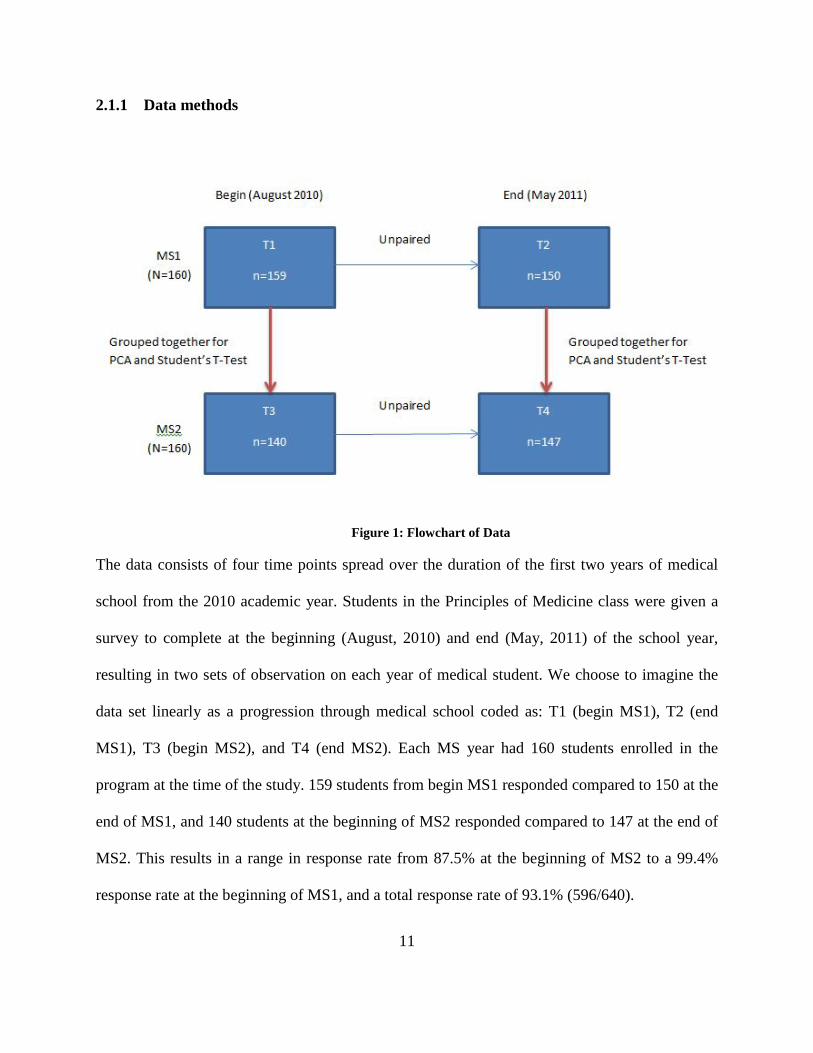
Figure 1: Flowchart of Data
The data consists of four time points spread over the duration of the first two years of medical
school from the 2010 academic year. Students in the Principles of Medicine class were given a
survey to complete at the beginning (August, 2010) and end (May, 2011) of the school year,
resulting in two sets of observation on each year of medical student. We choose to imagine the
data set linearly as a progression through medical school coded as: T1 (begin MS1), T2 (end
MS1), T3 (begin MS2), and T4 (end MS2). Each MS year had 160 students enrolled in the
program at the time of the study. 159 students from begin MS1 responded compared to 150 at the
end of MS1, and 140 students at the beginning of MS2 responded compared to 147 at the end of
MS2. This results in a range in response rate from 87.5% at the beginning of MS2 to a 99.4%
response rate at the beginning of MS1, and a total response rate of 93.1% (596/640).
11
As shown in Appendix B, the Institutional Review Board of SUNY Upstate Medical
University declared the study as exempt from review, due to deidentified data being presented in
aggregate form. Therefore, we cannot pair the responses of students from the beginning to end of
MS year. This creates the need to make sure assumptions of independence are not violated, as
any analysis performed within MS year will lack independence. However, MS1 and MS2 student
responses are completely independent, so we can focus our analysis on grouping together pairs
of time points from both MS years.
We decided to do two sets of analysis using two separate pairings of independent time
points. It was decided to pair both beginning of MS year time points (T1 and T3) together for
one pairing, and both end of MS year time points (T2 and T4) together for the other set of
analysis. It was determined that this set of pairings made the most sense in utilizing data from all
of the time points, as well as the responses being the most similar across MS year. Students at the
beginning of MS year are similar in that they are coming into the school year fresh and are
generally more optimistic as a result of not having acquired the stress, lack of sleep, and
cynicism that accumulates over the course of a school year. The same idea holds true for the end
of MS year grouping except that they have become worn out and less idealistic as they are
nearing the end of a difficult year. The pairings of time points also makes the most sense due to
the lack of comparability or clinical relevance of grouping the end of MS1 (T2) and beginning of
MS2 (T3) together.
For the Mann-Whitney U tests on the original items, we once again worked on pairing the
data in a clinically important way that preserved independence. Using these criteria, we chose to
compare T1 to T3, T1 to T4, and T2 to T4. We chose to exclude the other possible combinations
on the basis of a lack of independence or lack of relevance (T2 to T3).
12

For the principal component analysis (PCA) we utilized only the two pairings discussed
earlier (T1 and T3, T2 and T4), thus creating two separate sets of components. These
components were used for student’s t-test comparisons, as well as in ordinary least square (OLS)
regression. Since the PCA only generates components for the time points involved, we can only
run student’s t-tests on the components between the two time points from which they were
generated. The same holds true for selecting possible predictors in OLS regression, as the
predictors must come from the same time point PCA as the dependent variable. For the
regression analysis, missing values were excluded on a listwise basis. This means that only
observations with no missing values on any of the proposed predictors are used for the model.
This choice was supported by error messages in the output, which stated that some variables in
the model have impossible tolerances, and that “pairwise deletion may be inappropriate”. Thus,
listwise deletion of missing values was used for the regression analyses.
2.1.2 Survey Development
All of the matrix questions and items are described in the survey instrument displayed in
Appendix A. The survey consisted of 106 items divided into nine topic areas or matrices. The
nine topic areas developed corresponded to matrices in the survey.
1) Demographic data; 2) Do you anticipate working in the following settings? 3) How important are the following factors in considering your career in medicine? 4) How important are the opinions and experiences of others in considering your career in
medicine? 5) How likely are you to practice medicine in the following underserved populations,
specialties, or settings? 6) How likely are you to select the following for your specialty?
13

7) How important are the following factors in considering your choice for a specialty? 8) How important are the opinions and experiences of others in considering your choice for
a specialty? 9) Please indicate how much you agree or disagree with the following statements.
The items in matrix 1 consisted of a mixture of categorical choices (choices for marital
status are married, divorced, or single) and open ended responses (such as number of children)
for demographic information. The items in matrices 2,5, and 6 were ranked on a 5-item Likert
scale ranging from “Definitely No” to “Definitely Yes”. The items in matrices 3 and 4 were
ranked on 5-item Likert scales, ranging from “Not Important At All” (1) to “Very Important” (5).
The items from matrices 7 and 8 were ranked on a 5-item Likert scale ranging from “No
Influence” to “Strong Influence”. Matrix 9 was ranked using a 6-point Likert scale ranging from
“Completely Disagree” to “Completely Agree”, with “Neither Agree nor Disagree” as a central
anchor, and an additional “Not Sure” option. Responses to items marked “Not Sure” were
incorporated into the neutral anchor category (coded as 3).
A beta test period was not available, so the survey was designed with questions on similar
concepts interspersed throughout the instrument. This allowed for post-hoc calculation of
Cronbach’s α for related topics following the first administration of the instrument.
2.1.3 Survey Implementation
The survey was distributed during a mandatory clinical skills course for MS1s and MS2s in
August of 2010, at the beginning of the 2010-2011 academic year, and a second time, in May
2011, at the end of the 2010-2011 academic year. The Institutional Review Board of SUNY
14

Upstate Medical University determined this study exempt from review, because deidentified data
would be presented in aggregate form, and there was minimal risk associated with participation.
Students were verbally informed about the purpose of the survey, that their participation was
voluntary, and that their identities would not be linked to their responses.
2.2 METHODS OF COMPARISON
2.2.1 Mann-Whitney U Test
The Mann- Whitney U test is a powerful nonparametric equivalent to the student’s t-test, and is
used in comparing two unrelated samples of scores by evaluating the probabilities of the
distribution of ranking. [44] Our null hypothesis is that there is no difference between the ranks
of the two time points, versus the alternative that there is a significant difference between the
ranks of the two time points. In other words, we are testing if either of the two groups has
significantly lower or higher responses compared to the other group. [45] In this study, the
Mann-Whitney U test was used to compare separate, independent time points or compare
between other independent groups such as gender. The Mann-Whitney U test was chosen due to
the non-parametric distribution of responses, which was tested using the Shapiro-Wilk tests for
normality. All of the items in the survey came back with significant p- values for the tests for
normality, and thus we rejected the null hypothesis that the data were normally distributed. No
correction was made for multiple comparisons.
15
2.3 DATA REDUCTION
2.3.1 Principal Component Analysis (PCA)
Due to the size of the survey given to the students (over 100 items), we sought to reduce the total
number of items to analyze, without deleting original items from the analysis. Principal
components analysis (PCA) is a common tool in multivariate data analysis used to extract the
most important information from the data, and compress the size of the data set by keeping only
this information. [46] Instead of dealing with over 100 individual items, the goal of principal
components analysis is to create fewer components which contain the majority of the data’s
variation. [47] In essence, it trims down the redundant items that are measuring the same
underlying construct and turns them into a linear composite variable of the original items. [48] A
linear composite of items x, y, and z is given by ax + by + cz where a, b, and c are constants.
[49] Here, x, y, and z are the values for individual observations, and they are multiplied by
coefficients a, b, and c respectively to compute their composite score with the coefficients
chosen as discussed below.
For this study, principal component analysis was performed separately on each of the
nine individual question matrices of the survey (except for matrix 1), in an attempt to keep the
results more structured than putting all of the items into one massive principal components
analysis, which would result in items from different question matrices coming together in
components and lead to difficulty in identifying the “true” nature of the component. Typically,
when principal component analysis is performed, the extracted components are saved as new
variables for later use in regression analysis. [48]
16

PCA outputs several quantitative dependent variables called principal components, where
each principal component is orthogonal to the rest. [46, 47] The orthogonality of the principal
components means that each pair of vectors (principal components) is mutually perpendicular to
the others, and therefore independent. [50] The reason PCA is considered a data reduction
method is that the number of principal components is always less than or equal to the original
number of variables in the analysis. [46] The first principal component output will account for as
much of the variability in the data as possible, and each successive component will have the
largest variance possible under the condition that it is orthogonal to each of the preceding
components. [46]
Eigenvalues are the variances of the principal components, and when the PCA is run on
the correlation matrix (as is the case here), the values become standardized, and therefore each
variable has a mean of 0 and variance of 1. The orthogonalization of the components along with
the standardization converts nonparametric items into linear composite variables with a standard
normal distribution suitable for a student’s t-test instead of the Mann-Whitney U test [48].
The components extracted from the analysis contain information about the component
loadings, which are the correlations between the items (the original survey items) and the
component. The fact that these are correlations allows the component loadings to be between -1
and 1, and allows for easy understanding of the magnitude and direction (positive or negative) of
its association. Items which are correlated highly with each other typically come out on the same
component, and thus reflect a certain attitude or interest which has a broader scope than the
individual items of the survey. [46] Each component is given a name based upon the top loading
items, which reflect the topic that the correlated items are related to.
17

To help identify the broader topic of each component, rotation is utilized. Varimax
rotation, the most popular form, is a form of orthogonal rotation which generates a simpler
solution by creating a smaller number of large component loadings, and a large number of small
(or zero) component loadings. [46] The mathematical process involves searching for a linear
combination of the original items, such that the variance of the squared loadings is maximized.
[46] After varimax rotation, each original item tends to only be associated with one of the
components, and each component represents a smaller number of variables compared to a non-
rotated solution. [46] Varimax rotation does not alter the total amount of variation explained by
the model, but instead changes the individual contributions from the items so that they are easily
categorized as high loading or insignificantly loading. [46] This reorganizing of the contributions
is what allows for easier interpretation of a component’s underlying construct.
2.3.1.1 Student’s T-Test
Since the principal components are new variables composed of related constructs, it is of value to
attempt to find statistically significant differences between independent time points again.
However, the orthogonal transformation of the variables allows the use of the parametric
equivalent of the Mann- Whitney U test, the student’s t-test. The null hypothesis of the student’s
t-test is that two independent random samples have the same mean. [51] The student’s t-test used
was the two-sample independent t-test, for two different (therefore unpaired) groups of
participants and unknown population variance. [51, 52]
18
2.4 SCALE CREATION
2.4.1 Cronbach’s α
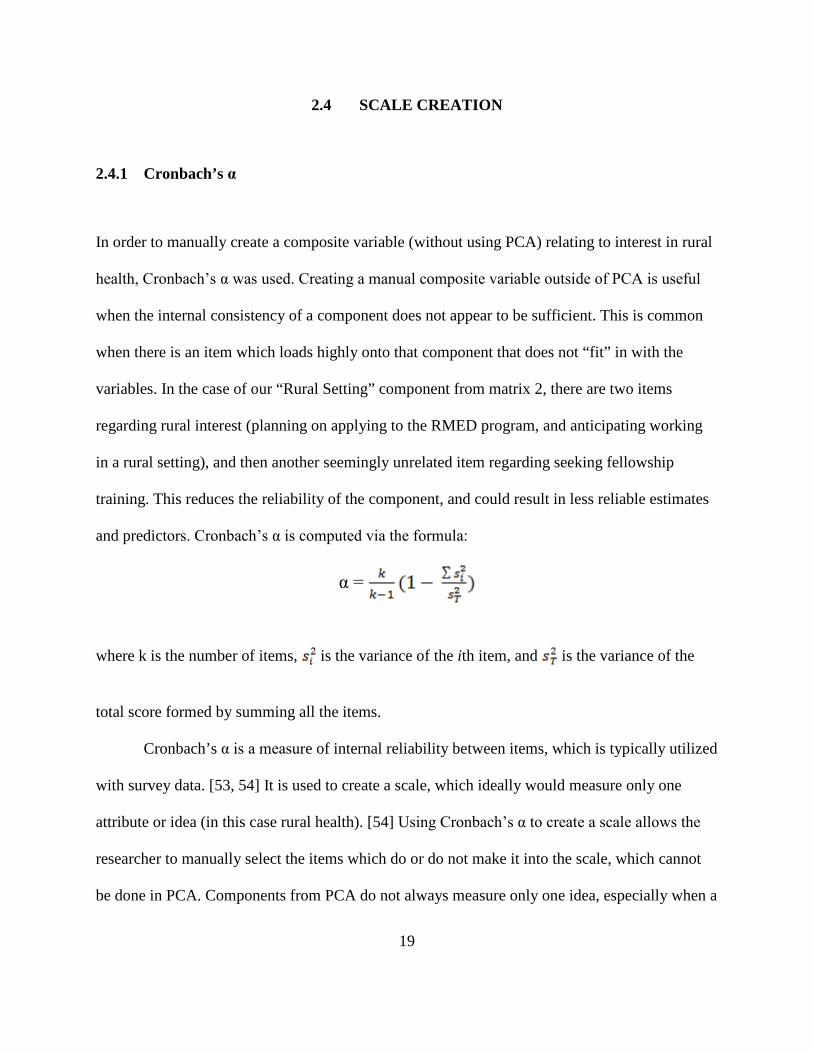
In order to manually create a composite variable (without using PCA) relating to interest in rural
health, Cronbach’s α was used. Creating a manual composite variable outside of PCA is useful
when the internal consistency of a component does not appear to be sufficient. This is common
when there is an item which loads highly onto that component that does not “fit” in with the
variables. In the case of our “Rural Setting” component from matrix 2, there are two items
regarding rural interest (planning on applying to the RMED program, and anticipating working
in a rural setting), and then another seemingly unrelated item regarding seeking fellowship
training. This reduces the reliability of the component, and could result in less reliable estimates
and predictors. Cronbach’s α is computed via the formula:
α =
where k is the number of items, is the variance of the ith item, and is the variance of the
total score formed by summing all the items.
Cronbach’s α is a measure of internal reliability between items, which is typically utilized
with survey data. [53, 54] It is used to create a scale, which ideally would measure only one
attribute or idea (in this case rural health). [54] Using Cronbach’s α to create a scale allows the
researcher to manually select the items which do or do not make it into the scale, which cannot
be done in PCA. Components from PCA do not always measure only one idea, especially when a
19
large amount of items are entered into the analysis. As a result, some components may be mostly
related to one topic, but then have a high loading (sometimes negative) item which does not
inherently fit with the overall topic of the component. A scale has internal consistency only to
the level in which all the items in the scale measure the same construct, and thus a scale
composed of highly related items will have a higher α statistic. [54] The α statistic ranges from 0
to 1 and measures the level to which items are measuring the same thing. Typically, the
researcher will develop a reasonable interval of items to use to create a scale, selecting from a set
of many items that may or may not relate to the construct. [54] In general, an α statistic of
between 0.70 and 0.80 is regarded as satisfactory in terms of the reliability of the scale created.
Often, scales created using Cronbach’s α are reinforced through principal component analysis, to
see if the scale created can be extracted into one component.
2.5 METHODS FOR FINDING PREDICTORS OF RURAL HEALTH
2.5.1 Ordinary Least Squares (OLS) Regression
In order to find predictors for future rural practice, ordinary least squares (OLS) regression was
utilized. OLS regression is a statistical method of analysis that estimates the relationship between
one or more independent variables and a dependent variable (future rural practice). [55] The
relationship is estimated by minimizing the sum of the squares in the difference between
observed and predicted values of our dependent variable configured as a linear line. [55] The
model for an OLS regression is:
20

Y = a + β1X1 + … β kXk + e
where Y is the dependent variable, a is the y-intercept, β is the slope and indicates the degree of
steepness of the straight line, X is the independent variable, and e represents the error. [55]
Several assumptions must be made and tested to use OLS regression. The assumptions
required for OLS regression include normally distributed residuals, linear relationships between
the dependent variable and independent variables, homoscedasticity of residuals, independence
of observations, no multicollinearity, and reliability of measures. [56] These assumptions are
tested using several different regression diagnostics. Common regression diagnostic analyses
include identifying outliers, leverage points, and influence points. Outliers are observations with
large residuals, which can substantially change the results of a regression. [57] Leverage points
are an observation with an extreme value on a predictor variable, usually deviating far from the
mean of that variable. [57] An observation is influential if removing that particular observation
significantly changes the estimate of coefficients. [57] Other diagnostics performed include
examining the normality of residuals (via Q-Q plots or Kolmogorov-Smirnov test), testing for
heteroscedasticity (via scatterplots of the residuals vs. predicted values), testing for collinearity
(via variance inflation factor [VIF] and looking for values above 10), and tests on nonlinearity
(via examining plots of the dependent against each independent variable for nonlinear patterns).
[57]
Advantages of OLS regression include that it has the maximum correlation between the
predicted and observed values of the outcome variable, and when errors are normally distributed,
OLS provides the most efficient estimators of unknown parameters for a linear regression model.
[58] For this study, the backward stepwise method of regression was used, which starts with a
full model, or one containing all possible variables, and removes each item from the starting
21

model. The regression calculation is performed to check the improvement in the residual sum of
squares for each of the resulting models compared to the starting model. When each model is
missing one term, the backward stepwise method selects the item associated with the highest p-
value as the first candidate for removal from the model. The item’s p-value is then compared to
the cut off p-value specified in the procedure, and if it is higher than the cut-off, the item is
removed from the regression model. This process continues until the highest candidate p-value is
not higher than the cut-off value, in which case the backward stepwise procedure will stop. A
threshold is set for the maximum p-value that is allowed in the model, and is usually set at p=.10,
as is the case in this study. [59] Therefore, the final model which is produced in the output is the
simplest model containing the most significant predictors. The enter method is also used to
manually include variables which may not make it into the model otherwise, but are chosen to
remain in the model regardless of significance level because of expansive literature confirming it
as a predictor. Enter method will enter all variables chosen into the model, regardless of
significance level.
22

3.0 APPLICATION OF METHODOLOGY
3.1 ANALYSIS PLAN
The four points of interest include responses from MS1s at the beginning and end of AY2010,
and MS2s at the beginning and end of AY2010. For purposes of simplicity and a linear timeline,
the four time points are coded as T1 (begin MS1), T2 (end MS1), T3 (begin MS2), and T4 (end
MS2). Although T1 and T3 are both occurring at the same time (August 2010), it helps to
imagine the change in medical student attitude over the course of medical school. The same idea
holds true for T2 and T4 (both occurred in May 2011). The analysis (except for the tests of
normality and Mann-Whitney U test) is grouped by two sets of two time points each, to account
for the lack of independence within MS year. The first grouping for analysis is the beginning of
each MS year (T1 and T3), and the other pair of time points for analysis is the end of each MS
year (T2 and T4). This eliminates the lack of independence issue which would be faced if all
results were analyzed simultaneously.
3.1.1 Comparisons of Original Survey Responses
Significant differences in survey responses between the four points of interest were analyzed in
nine dimensions:
23

For the present study, we utilized all nine matrix questions from the survey:
1. Differences between the four groups on responses to items that asked about demographic info;
2. Differences between the four groups on responses to items that asked about anticipated work setting;
3. Differences between the four groups on responses to items that asked about motivations for pursuing a career in medicine;
4. Differences between the four groups on responses to items that asked about the importance of others’ opinions in considering a career in medicine;
5. Differences between the four groups on responses to items that asked about the likelihood of practicing in underserved populations, specialties, or settings;
6. Differences between the four groups on responses to items that asked about the likelihood of working in a certain specialty;
7. Differences between the four groups on responses to items that asked about motivations for considering a specialty choice;
8. Differences between the four groups on responses to items that asked about the importance of others’ opinions in considering a specialty choice;
9. Differences between the four groups on responses to items that asked about attitudes towards primary care.
In addition to comparing between the two sets of two time points, comparisons were also
made between male and female students regardless of year in medical school. All groups were
compared on gender, marital status, race, Hispanic ethnicity, attending high school in the USA,
and rural background to assess comparability.
3.1.1.1 Tests of Normality (Shapiro-Wilk)
The individual items under each of the nine question matrices were tested for normality utilizing
the Shapiro-Wilk test for normality. [60] This is to determine whether the comparisons should be
made under nonparametric or parametric assumptions. Due to the data being unpaired, the tests
24

of normality will determine using either the student’s t-test (for parametric assumptions) or the
Mann-Whitney U test (for nonparametric assumptions) if there is a significant p-value.
3.1.1.2 Mann- Whitney U Test
The individual items under each of the nine question matrices were compared across each
combination of the four time points which were independent (T1 vs. T3, T1 vs. T4, T2 vs. T4),
as well as between gender (male vs. female). Comparisons were not made between T1 and T2,
and T3 and T4 due to a lack of independence, while comparisons were not made between T2 and
T3 due to lack of importance and oddity of comparing the time points (since there is no school
between the two time points, there is no effect besides a summer break, which does not seem to
be relevant to study). Given the ordinal nature and non-normal distribution (tested using Shapiro-
Wilk test for normality) of the data, we utilized the Mann-Whitney U test to assess significance
of any differences. No correction was made for multiple comparisons.
3.1.2 Data Reduction via Principal Components Analysis
We created linear composite variables (LCVs) for the items under each question matrix via
principal components analysis (PCA). Components exceeding an Eigenvalue of 1 were extracted
from the analysis, and solutions were assessed after varimax rotation. An Eigenvalue greater than
or equal to 1 is the default setting for the SPSS program, and varimax rotation attempts to
maximize the variance of each of the factors, so the total amount of variance accounted for is
redistributed over the extracted factors. Each component was given a name based upon the
highest loading items, and saved as a new variable into the dataset. For example, the LCV which
25
was generated in the beginning of MS year analysis titled “Rural Setting” had three variables
which loaded highly onto the component, with the two highest being interest in applying to the
Rural Medical Education Program (RMED) and anticipation of working in a rural setting. The
third high loading variable involved seeking fellowship training after residency, but had a lower,
negative loading. Thus, the component mostly deals with issues of interest in rural work,
therefore we gave it the generalized title “Rural Setting”. This process was repeated for each
principal component generated for both analyses.
Since the four time points are not independent from each other, we chose to run two
separate PCA’s, one combining T1 and T3, and the combining T2 and T4. The components from
both PCA’s were saved as linear composite for use predictors in regression, with each
component having a mean of 0 and a variance of 1. All principal components are normally
distributed and independent of the other factors extracted from the same question matrix.
3.1.2.1 Two Independent Sample Student’s T-test
The two groups of time points T1and T3, and T2 and T4 were compared across the linear
composite variables extracted through PCA, using a Student’s t-test to assess significance of any
observed differences between mean factor scores in the four time periods. Each PCA only
created composite scores for the two time points involved (T1 and T3 or T2 and T4). The linear
composite variables encompass larger constructs compared to the original variables, thus it is
check for significant differences over time for these broader topics.
26
3.1.3 Finding significant predictors for future rural practice
3.1.3.1 Finding significant demographic predictors for future rural practice
To test the robustness of results, factors relating to rural health were entered into a backward
stepwise ordinary least squares (OLS) linear regression procedure (with entry as .05, and
removal of .10), in an attempt to model the effect of demographic information (such as gender,
MS1 or MS2, marital status, Hispanic, race, and rural upbringing). Each predictor was entered as
a dummy variable in models following the form:
Factor=Constant + βk…I Covariates
a. Year/ Time: MS2 =1 / Non-MS2 = 0
b. Race: White/ Caucasian = 1 / Non-White = 0
c. Ethnicity: Hispanic = 1 / Not Hispanic = 0
For the rural/ urban variable, students were characterized using the Rural-Urban
Commuting Area (RUCA) based on the zip code where the student attended secondary school.
[61] RUCA scores of 1.0, 1.1, 2.0, 2.1, 3.0, 4.1, 5.1, 7.1, 8.1, and 10.1 are categorized as urban,
and scores of 4.0, 4.2, 5.0, 5.2, 6.0, 6.1, 7.0, 7.2, 7.3, 7.4, 8.0, 8.2, 8.3, 8.4, 9.0, 9.1, 9.2, 10.0,
10.3, 10.4, 10.5, and 10.6 were categorized as rural. [61] The scores were coded dichotomously
into either the rural or urban category, creating the dummy variable:
d. Rural = 1, Non-Rural = 0 e. Urban = 1, Non-Urban = 0
f. Marital Status: Married = 1 / Not Married = 0
27

3.1.3.2 Finding significant demographic and attitude predictors for future rural practice
Principal components (minus those in the same question matrix (2) as the dependent variable)
and demographic variables (such as gender, race, marital status, Hispanic ethnicity, year in
medical school, and rural background) were entered into a backward stepwise ordinary least
squares (OLS) linear regression procedure using the “Rural Setting” principal component as a
dependent variable (with entry as .05, and removal of .10). Removing the components (“Global
Setting”, “Suburban/ Non-Metro Setting”, and “U.S. Setting”) from the same matrix as the
dependent variable is to take into account that these components diverged from each other for a
reason and that they are completely orthogonal to one another. The form of the regression model
is as follows:
Factor = β0+β1X1 + β2X2 + … + βkXk +
3.1.4 Creation of a new rural dependent variable
3.1.4.1 Creating the scale using Cronbach’s α
A linear composite variable was created using Cronbach’s α which contained those items
believed to best encompass interest in working in rural health. The reliability of the composite
variable was tested using Cronbach’s α, and items were added/ removed until reliability was
maximized. A total of five items ended up in the scale, which is a reasonable number to compose
a scale. Items were considered (added) for the scale based on their perceived relevance to rural
setting, which involved the question mentioning rural, global, or underserved populations in the
text. Items were removed using the option in SPSS which outputs the Cronbach α statistic, along
with the α statistic for the removal of each item. Trial and error were used to obtain the optimal
28
scale. The five items included in the scale include “Do you anticipate working in a rural
community?”, “Are you planning on applying to the RMED program?”, “How likely are you to
practice in the rural poor population?”, “How likely are you to practice medicine in a full-time
practice in a rural location?”, and “How likely are you to practice medicine in an underserved
geographic area?”. The five items resulted in a respectable Cronbach’s α of .780. Items were
selected across all question matrices. The five items came from two different matrices, one
which asked about anticipated work setting (2) and the other asked about likelihood to work in
underserved populations or geographic areas (5).
3.1.4.2 Turning the scale into a linear composite variable via Principal Components
Analysis
These five items were then used to create linear composite variables via PCA, extracting factors
that exceeded an Eigenvalue of 1, and assessing solutions after varimax rotation. As stated
before, two separate PCA’s were performed to avoid violating independence. The factors were
then saved as linear composite variables into the data set for purposes of using in principal
components regression, each with a mean of 0 and a standard deviation of 1. These linear
composite variables were then used as dependent variables to see if these “better” composite
variables provided any new significant predictors when compared to the previous results.
3.1.4.3 Finding significant demographic predictors for the new rural dependent variable
The manually created linear composite variable (one for the beginning of MS year, and the other
for the end of MS year) was then entered into a backward stepwise ordinary least squares (OLS)
linear regression procedure as the dependent variable (with entry as .05, and removal of .10).
29

Here, the effect of demographic information was modeled as predictors for future rural practice.
Principal components from the same question matrix as the “Rural Setting” component were not
entered into the analysis for the purposes of making the results between the two regressions as
comparable as possible.
3.1.4.4 Finding significant demographic and attitude predictors for the new rural
dependent variable
Principal components (minus those in the same question matrix as the dependent variable) and
demographic variables were entered into a backward stepwise ordinary least squares (OLS)
linear regression procedure using the manually created rural interest principal component as a
dependent variable (with entry as .05, and removal of .10). The form of the regression model is
as follows:
Factor = β0+β1X1 + β2X2 + … + βkXk +
3.1.5 Analyzing final models with regression diagnostics
Basic regression diagnostic analyses will be performed on the final models including identifying
outliers, leverage points, and influence points. Diagnostics on the assumptions of the model
performed include examining the normality of residuals (via Q-Q plots or Kolmogorov-Smirnov
test), testing for heteroscedasticity (via scatterplots of the residuals vs. predicted values), testing
for collinearity (via variance inflation factor [VIF] and looking for values above 10), and tests on
nonlinearity (via examining plots of the dependent against each independent variable for
nonlinear patterns).
30

The analysis was performed using SPSS v. 19.0 statistical software. Statistical significance was
< 0.05 and borderline statistical significance 0.05-0.10.
31
4.0 RESULTS
4.1.1 Comparability between MS1 and MS2, as well as to national statistics
A total of 306 MS1s (n=159) and MS2s (n=147) responded, out of approximately 320 potential
respondents (160 MS1 / 160 MS2), yielding a 95.6% response rate. The response rates at the four
individual time points (T1, T2, T3, T4) ranged from 87.5% (n=140) for T3 to 99.4% (n=159) for
T1, and a 93.1% overall response rate (596/640). As shown in Table 1, the sample comprised of
approximately 54% male students and 66% self-identified white/ Caucasians. Only eight students
between the two beginning of medical school years (n = 291) self-identified as Hispanic. The
sample was 88% single, and 78% were of urban origin according to the RUCA classification
system. The two medical school years were very similar, with statistically significant differences
only between the number of self-identified Hispanic students in MS1 (MS1=7, MS2 =1; χ2 =
3.727, p = .054*), and more married students in MS2 (MS1=6, MS2 = 23; χ2 = 14.482, p
=.001).Additionally, the student body is more white (65.5% vs. 54.6% nationally in 2012; p
<.001) than the nation as a whole.
32
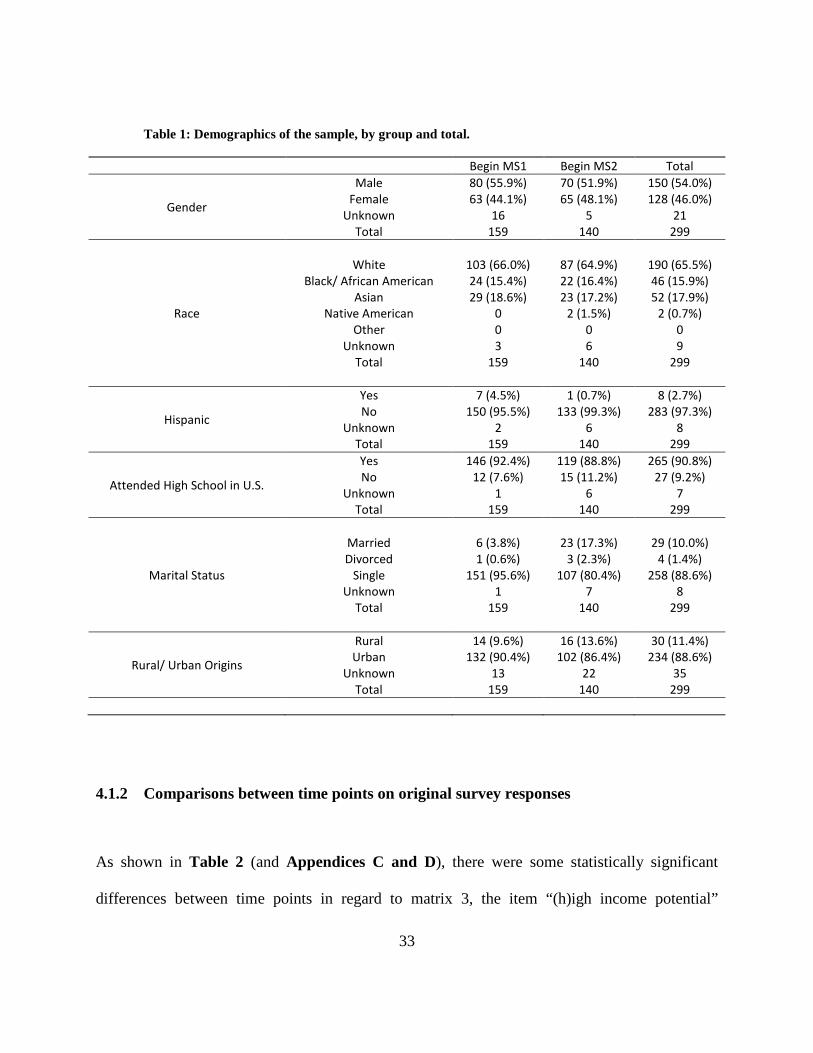
Table 1: Demographics of the sample, by group and total.
Begin MS1 Begin MS2 Total
Gender
Male Female
Unknown Total
80 (55.9%) 63 (44.1%)
16 159
70 (51.9%) 65 (48.1%)
5 140
150 (54.0%) 128 (46.0%)
21 299
Race
White Black/ African American
Asian Native American
Other Unknown
Total
103 (66.0%) 24 (15.4%) 29 (18.6%)
0 0 3
159
87 (64.9%) 22 (16.4%) 23 (17.2%)
2 (1.5%) 0 6
140
190 (65.5%) 46 (15.9%) 52 (17.9%)
2 (0.7%) 0 9
299
Hispanic
Yes No
Unknown Total
7 (4.5%) 150 (95.5%)
2 159
1 (0.7%) 133 (99.3%)
6 140
8 (2.7%) 283 (97.3%)
8 299
Attended High School in U.S.
Yes No
Unknown Total
146 (92.4%) 12 (7.6%)
1 159
119 (88.8%) 15 (11.2%)
6 140
265 (90.8%) 27 (9.2%)
7 299
Marital Status
Married Divorced
Single Unknown
Total
6 (3.8%) 1 (0.6%)
151 (95.6%) 1
159
23 (17.3%) 3 (2.3%)
107 (80.4%) 7
140
29 (10.0%) 4 (1.4%)
258 (88.6%) 8
299
Rural/ Urban Origins
Rural Urban
Unknown Total
14 (9.6%) 132 (90.4%)
13 159
16 (13.6%) 102 (86.4%)
22 140
30 (11.4%) 234 (88.6%)
35 299
4.1.2 Comparisons between time points on original survey responses
As shown in Table 2 (and Appendices C and D), there were some statistically significant
differences between time points in regard to matrix 3, the item “(h)igh income potential”
33
experienced significant or marginally significant increased importance over nearly every time
point combination. Similarly, those farther along in medical school were significantly more
likely to place importance on “(a)vailability of jobs” and “(s)tatus of physicians”.
Students indicated a decreased interest in matrix 5 for all items except for “(e)mergency
medicine” from beginning of MS1 to end of MS2. Significant or nearly significant declines were
observed for “(g)lobal health”, “(p)ublic health service”, and “(g)eneral surgery” among others.
Interest in specialties related to primary care and rural health needs also experienced significant
declines in response to items in matrix 6. Students at the beginning of MS1 were more likely to
be interested in “(f)amily medicine”, “(o)bstetrics and Gynecology”, and “(p)reventative
medicine” than they were as they progressed through their pre-clinical years.
In response to items in matrix 7, students at the beginning of MS1 were less likely to
place importance on “(i)ncome expectations for the specialty”, “(p)restige of the specialty I am
considering”, and “(a)bility to balance my work life with my family responsibilities” than those
later in medical school. Attitudes towards primary care topics and issues were also split between
the four time points. Students at the beginning of MS1 were in lesser agreement that “(p)rimary
care doctors mostly manage chronic health problems”, “(p)rimary care is not very intellectually
stimulating”, and “(p)rimary care doctors have a large work overload”.
34

Table 2: Mann-Whitney U comparison of begin MS1 and end MS2 on question matrices
(Matrix) Top Question Variable T1 T4 Sig. Level Trend
(3) How important are the following factors in considering your career in
medicine?
• Desire to do primary care 3.04 2.75 .054 Decreasing
• Availability of jobs 3.55 3.84 .020 Increasing
• Opportunity to help patients who are socially disadvantaged
4.17 3.90 .027 Decreasing
• High income potential 2.82 3.32 .000 Increasing
(5) How likely are you to practice medicine in the following underserved
populations, specialties, or settings?
• Global Health, via temporary medical missions
3.72 3.27 .002 Decreasing
• Public Health Service (Loan Payback)
2.85 2.47 .001 Decreasing
• Obstetrics/ Gynecology 2.36 1.98 .000 Decreasing
• General Surgery 2.91 2.49 .001 Decreasing
• Psychiatry 2.25 1.99 .006 Decreasing
• Emergency Medicine 2.86 3.10 .023 Increasing
(7) How important are the following factors in considering your choice for a
specialty?
• Income expectations for the specialty
2.81 3.23 .003 Increasing
• Ability to balance my work life with my family responsibilities
4.37 4.60 .020 Increasing
• Length of residency training associated with the specialty
3.18 3.48 .029 Increasing
(9) Please indicate how much you agree or disagree with the following
statements.
• Preventative knowledge is essential for all medical students to learn
4.83 4.53 .000 Decreasing
• Primary care doctors mainly manage chronic health problems
3.26 3.79 .000 Increasing
• It is impossible to be an expert in such a wide field as primary care
2.69 3.01 .022 Increasing
• Primary care is not very intellectually stimulating
1.90 2.22 .005 Increasing
• Primary care doctors have a large work overload
3.63 3.95 .008 Increasing
35

4.1.3 Principal Components Analysis
Principal Components Analyses at the beginning of MS year and end of MS year extracted
between 3 to 8 linear composite variables for each of the nine matrices, except for the two
matrices (4 and 8) which dealt with the importance of others opinions and experiences on their
specialty choice or career in medicine, which only extracted one linear composite variable. The
important extracted linear composite variables for both PCA analyses are displayed in
Appendices E and F, and those with statistically significant t-test comparisons between the two
time points are displayed in Table 3 (T1 and T3) and Table 4 (T2 and T4).
36

Table 3: Statistically significant differences of components from beginning MS1 to beginning MS2
Components Items (loading score) Mean LCV/ Time (sig.)
(2) Do you anticipate working in the following settings?
Rural Setting
• Are you planning on applying to the RMED program (.730)
• In a rural community (.701)
• Are planning on seeking fellowship training after residency (-.665)
T1: .1207 T3: -.1489
(.025)
(3) How important are the following factors in considering your career in medicine?
Employment Benefits
• Job security (.827)
• Availability of jobs (.806)
• High income potential (.755)
• Status of physicians (.558)
T1: -.1727 T3: .2041
(.001)
Idealism in Medicine
• Opportunity to help patients who are socially disadvantaged (.783)
• Desire to serve my community (.731)
• Desire to do primary care (.611)
• Opportunities to make a difference in people’s lives (.564)
T1: .1180 T3: -.1394
(.029)
(5) How likely are you to practice medicine in the following underserved populations, specialties, or settings?
OBG and Psychiatry
• Obstetrics/ Gynecology (.826)
• Psychiatry (.606)
T1: .2694 T3: -.3132
(<.0001)
(7) How important are the following factors in considering your choice for a specialty?
Lifestyle/ Family Considerations
• The lifestyle of the specialty I am considering (.817)
• Ability to balance my work life with my family responsibilities (.787)
• Length of residency training associated with the specialty (.571)
T1:-.1317 T3: .1564
(.016)
(9) Please indicate how much you agree or disagree with the following statements.
Negative/ Antagonistic View of Primary Care
• Primary care doctors mostly manage chronic health problems (.812)
• It is impossible to be an expert in such a wide field as primary care (.692)
• I am more interested in learning the skills required for my chosen specialty rather than a general set of clinical practice skills. (.532)
T1: -.2077 T3: .2463 (<.0001)
Negative/ Sympathetic View of Primary Care
• Primary care doctors are poorly valued by the rest of the medical profession (.802)
• Primary care doctors have a large work overload (.770)
T1: -.1517 T3: .1799 (<.0001)
37

Table 4: Statistically significant differences of components from end MS1 to end MS2
Components Items (loading score) Mean LCV/ Time (sig.)
(2) Do you anticipate working in the following settings?
Rural Setting
• Are you planning on applying to the RMED program (.787)
• In a rural community (.772)
• Are planning on seeking fellowship training after residency (-.624)
T2: .1198 T4: -.1251
(.042)
(5) How likely are you to practice medicine in the following underserved populations, specialties, or settings?
OBG/ Psychiatry
• Obstetrics/ Gynecology (.858)
• Psychiatry (.657)
T2: .1566 T4: -.1635
(.007)
(7) How important are the following factors in considering your choice for a specialty?
Lifestyle/ Family Considerations
• The lifestyle of the specialty I am considering (.814)
• Ability to balance my work life with my family responsibilities (.806)
• Length of residency training associated with the specialty (.509)
T2: -.0175 T4: .1819
(.002)
(9) Please indicate how much you agree or disagree with the following statements
Negative/ Antagonistic View of Primary Care
• Primary care doctors mostly manage chronic health problems (.781)
• It is impossible to be an expert in such a wide field as primary care (.767)
• I am more interested in learning the skills required for my chosen specialty rather than a general set of clinical practice skills (.403)
T2: -.1823 T4: .1811
(.002)
Negative/ Sympathetic View of Primary Care
• Primary care doctors have a large work overload (.808)
• Primary care doctors are poorly valued by the rest of the medical profession (.785)
T2: -.2051 T4: .2037
(.001)
4.1.4 Student t-test comparisons between time points on extracted principal components
As shown in Tables 3 and 4, students at the beginning of MS1 (T1) were more likely to consider
idealism as a motivator to pursue a career in medicine than at the beginning of MS2 (p=.029).
Students were more likely to consider working in a rural setting at the beginning of MS1
38

compared to beginning of MS2 (p =.025), as well as having less negative antagonistic and
sympathetic thoughts towards primary care (Negative Antagonistic: p <.0001, Negative
Sympathetic: p <.0001). Additionally, students at the beginning of MS2 were more likely to
place importance on employment benefits and income (p =.001) and lifestyle considerations
(p =.016) when considering a career in medicine, when compared to students at the beginning of
MS1.
Students at the end of MS2 were significantly more likely to place importance on lifestyle
and family considerations for their specialty than students at the end of MS1 (p =.002). Students
finishing MS2 also had significantly more negative attitudes and perceptions of working in
primary care (Negative Antagonistic: p =.002, Negative Sympathetic: p =.001) than students at
the end of MS1. Students at the end of MS1 were also significantly more likely to consider
working in a rural setting when compared to students at the end of MS2 (p =.042).
4.1.5 Ordinary Least Squares Regression on “Rural Setting” linear composite variable
4.1.5.1 Using demographic predictors
As shown in Table 5, using only demographic factors as predictors in the backward stepwise
OLS regression analyses on the LCV relating to anticipated work in a rural setting, revealed
similar predictors for both the beginning and end of MS year analysis. Regression for the
beginning of MS year indicated that interest in working in a rural setting was higher among
married students (β = .530, p =.019) and students with a rural upbringing (β = .754, p <.0001),
but interest was decreased as a result of advancing to MS2 (β = -.370, p =.005). Conversely,
regressions for the end of MS year indicated that interest in working in a rural setting was higher
39

among whites (β = .242, p =.083), married students (β =.527, p =.018), and students from a rural
upbringing (β = .806, p <.0001), while advancing to MS2 decreased interest in working in a rural
location (β = -.295, p =.021).
.
Table 5: Results of backward stepwise linear regression analysis using only demographics.
Dependent Variable: Rural Setting (T1T3) Predictors β (significance level) Model Summary Constant .036 (.694)
R2 = .098 F= 8.286 (<.0001)
Marital Status .530 (.019) Rural Upbringing .754 (<.0001)
MS year 2 -.370 (.005) Dependent Variable: Rural Setting (T2T4)
Predictors β (significance level) Model Summary Constant -.158 (.242)
R2 = .133 F = 8.815 (<.0001)
Race .242 (.083) Marital Status .527 (.018)
Rural Upbringing .806 (<.0001) MS Year 2 -.295 (.021)
4.1.5.2 Using extracted principal components
Table 6 shows the results of backward stepwise OLS regression analyses for students at the
beginning and end of MS year on the LCV relating to anticipated work in a rural setting using
only the extracted principal components as predictors. Among attitudes that increase the
likelihood of practicing in a rural setting for students at the beginning of an MS year are interest
in working with rural underserved/ Native American populations (β =.523, p <.0001), interest in
practicing OBG or psychiatry specialties (β =.322, p =.006), and importance of others opinions
and experiences in choice of specialty (β =.241, p =.043). Conversely, attitudes that decrease the
likelihood of practicing in a rural setting are importance of others opinions in considering a
career in medicine (β =-.213, p =.067), interest in practicing a technology focused specialty
(β =-.230, p =.078), importance of prestige and income in considering specialty (β = -.207,
40

p=.084), importance of specialty content in choosing specialty (β =-.267, p =.051), and perceived
value of primary care skills (β =-.214, p =.017).
At the end of MS year, working in rural underserved populations and primary care
(β =.535, p <.0001) and interest in working in OBG/ Psychiatry specialty (β=.290, p=.002) were
statistically significantly increased. Among attitudes which decreased anticipation of working in
a rural setting were interest in working in community health (β =-.204, p =.087), interest in
working with incarcerated/ disabled populations (β =-.360, p <.0001), and importance of prestige
and income of specialty (β =-.372, p =.001).
Table 6: Results of backward stepwise linear regression analysis using only LCV.
Dependent Variable: Rural Setting (T1T3) Predictors β (sig. level) Model Summary
Constant .079 (.443)
R2 = .604 F= 9.933 (<.0001)
Opinions of career in medicine -.213 (.067) Rural / Native American Population .523 (<.0001) OBG/ Psychiatry .322 (.006) Technology Specialty -.230 (.078) Prestige and Income -.207 (.084) Content Interest -.267 (.051) Opinions of Specialty Choice .241 (.043) Value of Primary Care Skills -.214 (.017)
Dependent Variable: Rural Setting (T2T4) Predictors β (sig. level) Model Summary
Constant .083 (.377)
R2 = .623 F=16.587 (<.0001)
Rural/ Primary Care .535 (<.0001) Community Health -.204 (.087) Incarcerated and Disabled -.360 (<.0001) OBG/ Psychiatry .290 (.0002) Prestige and Income -.372 (.001)
4.1.5.3 Using demographic information and linear composite variables
Table 7 shows the results of the combined demographic and LCV analyses for the beginning and
end of MS year. Among beginning of MS year attitudes that increased the likelihood of future
practice in a rural location were female gender (β =.392, p =.080), importance of employment
41

benefits and income in considering a career in medicine (β =.359, p =.008), interest in working
with underserved poor populations (β =.263, p =.049), interest in working with rural/ Native
American populations (β =.708, p <.0001), likelihood of practicing obstetrics and gynecology (β
=.264, p =.007), and interest in working in emergency/ family medicine (β =.214, p =.054).
Conversely, attitudes that decreased the likelihood of future rural practice were interest in
internal medicine specialty (β =-.214, p =.024), importance of prestige and income in specialty
choice (β =-.353, p =.001), and importance of lifestyle and family considerations in specialty
choice (β =-.240, p =.014).
At the end of MS year, interest in working with rural populations and primary care
practice (β =.363, p <.0001), interest in OBG/ Psychiatry specialty (β =.254, p =.004), and being
from a rural area (β =1.596, p <.0001) statistically significantly increased likelihood of future
rural practice. Interest in working with incarcerated/ disabled groups (β =-.264, p =.004),
importance of prestige and income in specialty choice (β =-.226, p =.015), and perceived value
of primary care skills (β =-.114, p =.083) all statistically significantly decreased the likelihood of
future rural practice.
42
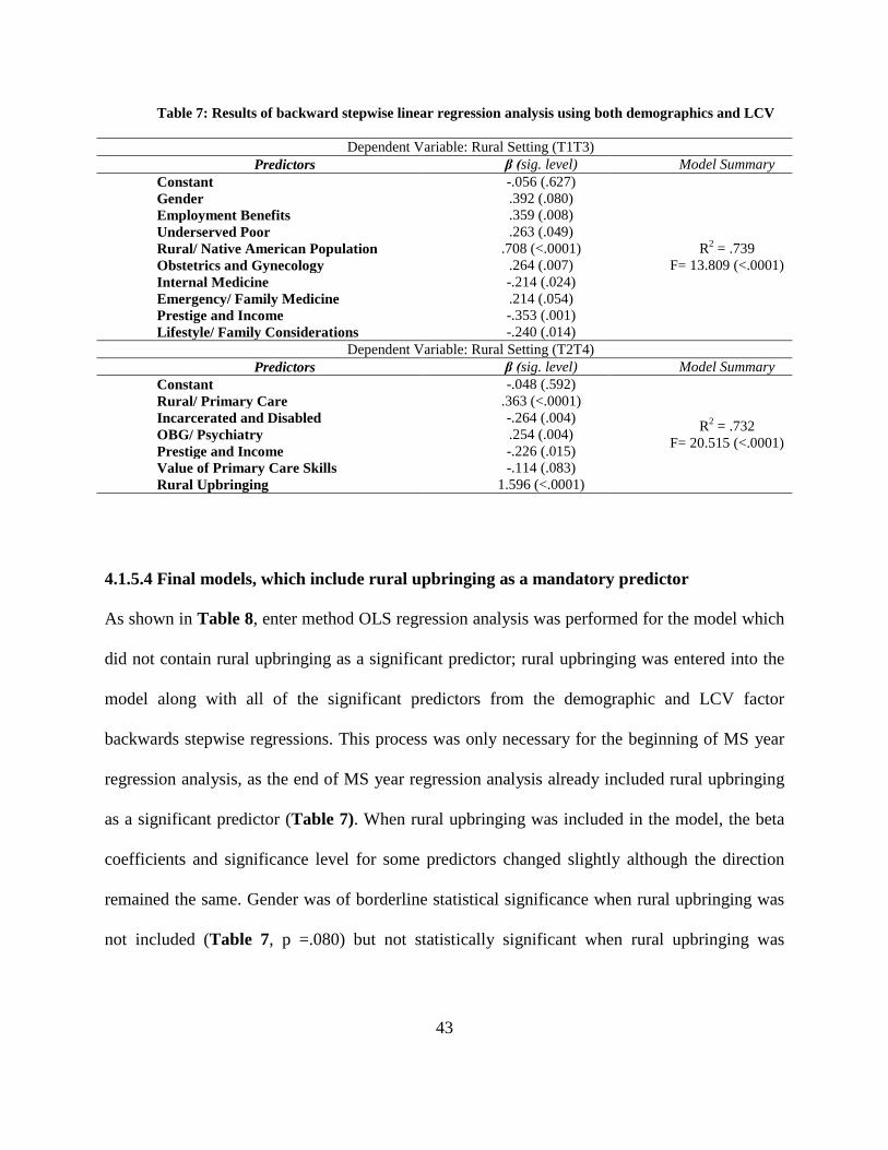
Table 7: Results of backward stepwise linear regression analysis using both demographics and LCV
Dependent Variable: Rural Setting (T1T3) Predictors β (sig. level) Model Summary
Constant -.056 (.627)
R2 = .739 F= 13.809 (<.0001)
Gender .392 (.080) Employment Benefits .359 (.008) Underserved Poor .263 (.049) Rural/ Native American Population .708 (<.0001) Obstetrics and Gynecology .264 (.007) Internal Medicine -.214 (.024) Emergency/ Family Medicine .214 (.054) Prestige and Income -.353 (.001) Lifestyle/ Family Considerations -.240 (.014)
Dependent Variable: Rural Setting (T2T4) Predictors β (sig. level) Model Summary
Constant -.048 (.592)
R2 = .732 F= 20.515 (<.0001)
Rural/ Primary Care .363 (<.0001) Incarcerated and Disabled -.264 (.004) OBG/ Psychiatry .254 (.004) Prestige and Income -.226 (.015) Value of Primary Care Skills -.114 (.083) Rural Upbringing 1.596 (<.0001)
4.1.5.4 Final models, which include rural upbringing as a mandatory predictor
As shown in Table 8, enter method OLS regression analysis was performed for the model which
did not contain rural upbringing as a significant predictor; rural upbringing was entered into the
model along with all of the significant predictors from the demographic and LCV factor
backwards stepwise regressions. This process was only necessary for the beginning of MS year
regression analysis, as the end of MS year regression analysis already included rural upbringing
as a significant predictor (Table 7). When rural upbringing was included in the model, the beta
coefficients and significance level for some predictors changed slightly although the direction
remained the same. Gender was of borderline statistical significance when rural upbringing was
not included (Table 7, p =.080) but not statistically significant when rural upbringing was
43

included (Table 8, p =0.176); the statistical significance of other predictors did not change with
the addition of rural upbringing.
Table 8: Results of enter method linear regression, where rural upbringing is a mandatory predictor.
Dependent Variable: Rural Setting (T1T3) Predictors β (sig. levell) Model Summary
Constant -.034 (.770)
R2 = .732 F= 12.013 (<.0001)
Rural Upbringing .282 (.414) Gender .314 (.176) Employment Benefits .388 (.005) Underserved Poor .236 (.077) Rural/ Native American Population 645 (<.0001) Obstetrics and Gynecology .253 (.011) Internal Medicine -.205 (.033) Emergency/ Family Medicine .213 (.062) Prestige and Income -.384 (<.0001) Lifestyle/ Family Considerations -.221 (.028)
4.2 ANALYSIS OF NEW MANUALLY CREATED RURAL COMPOSITE
DEPENDENT VARIABLE
4.2.1 Ordinary Least Squares Regression on demographic predictors
The intermediate results for inclusion of the demographic factors only are shown in Appendix H
and those for only the extracted principal components are shown in Appendix I. Appendix H
shows the results of the backward stepwise OLS regression analyses at the beginning and end of
MS year on the manually created rural location LCV, using only demographic factors as
predictors. For students at the beginning of their MS year, it was found that being married (β
44
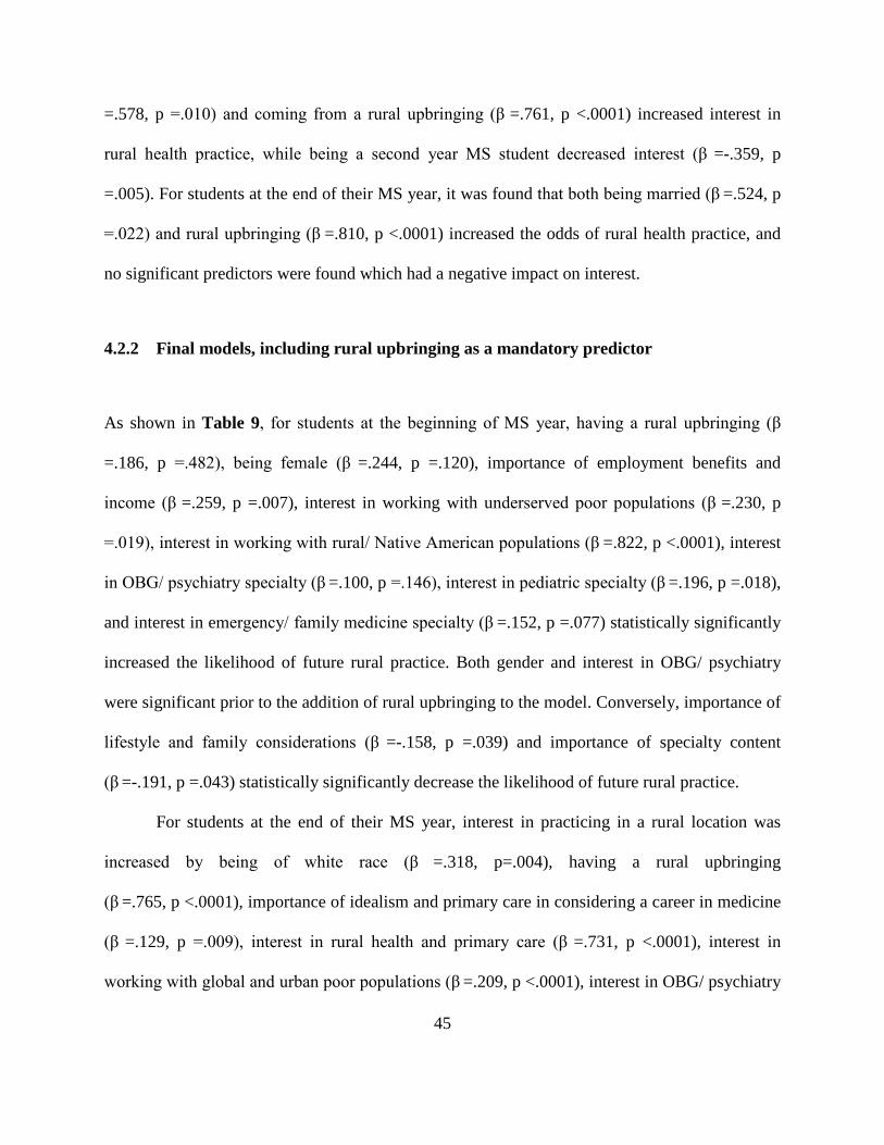
=.578, p =.010) and coming from a rural upbringing (β =.761, p <.0001) increased interest in
rural health practice, while being a second year MS student decreased interest (β =-.359, p
=.005). For students at the end of their MS year, it was found that both being married (β =.524, p
=.022) and rural upbringing (β =.810, p <.0001) increased the odds of rural health practice, and
no significant predictors were found which had a negative impact on interest.
4.2.2 Final models, including rural upbringing as a mandatory predictor
As shown in Table 9, for students at the beginning of MS year, having a rural upbringing (β
=.186, p =.482), being female (β =.244, p =.120), importance of employment benefits and
income (β =.259, p =.007), interest in working with underserved poor populations (β =.230, p
=.019), interest in working with rural/ Native American populations (β =.822, p <.0001), interest
in OBG/ psychiatry specialty (β =.100, p =.146), interest in pediatric specialty (β =.196, p =.018),
and interest in emergency/ family medicine specialty (β =.152, p =.077) statistically significantly
increased the likelihood of future rural practice. Both gender and interest in OBG/ psychiatry
were significant prior to the addition of rural upbringing to the model. Conversely, importance of
lifestyle and family considerations (β =-.158, p =.039) and importance of specialty content
(β =-.191, p =.043) statistically significantly decrease the likelihood of future rural practice.
For students at the end of their MS year, interest in practicing in a rural location was
increased by being of white race (β =.318, p=.004), having a rural upbringing
(β =.765, p <.0001), importance of idealism and primary care in considering a career in medicine
(β =.129, p =.009), interest in rural health and primary care (β =.731, p <.0001), interest in
working with global and urban poor populations (β =.209, p <.0001), interest in OBG/ psychiatry
45

specialty (β =.185, p<.0001), interest in surgery specialty (β =.085, p=.090), and importance of
specialty content (β =.124, p=.019). There were no statistically significant negative predictors in
this model.
Table 9: Results of enter method linear regression for new dependent variable, where rural
upbringing is a mandatory predictor.
Dependent Variable: Manually Created Rural Setting LCV (T1 and T3) Predictors β (sig. level) Model Summary
Constant -.083 (.346)
R2 = .789 F= 17.537 (<.0001)
Rural Upbringing .186 (.482) Gender .244 (.120) Employment Benefits .259 (.007) Underserved Poor .230 (.019) Rural/ Native American Population .822 (<.0001) OBG/ Psychiatry .100 (.146) Pediatric Specialty .196 (.018) Emergency/ Family Medicine .152 (.077) Lifestyle/ Family Considerations -.158 (.039) Content Interest -.191 (.043)
Dependent Variable: Manually Created Rural Setting LCV (T2 and T4) Predictors β (sig. level) Model Summary
Constant -.265 (.003)
R2 = .911 F= 58.705 (<.0001)
Idealism and Primary Care .129 (.009) Rural/ Primary Care .731 (<.0001) Global/ Urban Poor .209 (<.0001) OBG/ Psychiatry .185 (<.0001) Surgery Specialty .085 (.090) Content Interest .124 (.019) White Race .318 (.004) Rural Upbringing .765 (<.0001)
46

4.3 FINAL MODEL REGRESSION DIAGNOSTICS
Figure 2 displays the plot of leverage versus studentized deleted residual value for all four
models, and Figure 3 shows the QQ-plot for model 2 displaying its non-normally distributed
residuals.
Figure 2: Leverage vs. Studentized Deleted Residuals Plot
47
Figure 3: Model 2 (T2T4 Rural Setting) QQ Plot
Model 1 (T1T3 Rural Setting), 3 (T1T3 Manually Created Rural LCV), and 4 (T2T4 Manually
Created Rural LCV) showed no cause for concern as a result of regression model diagnostics. All
three models had few outliers, leverage points, or influential points. Of the points that were
outliers, leverage points, or influential points, none were especially problematic in being
considerably past the cut-off value for identification, nor were any observations problematic on
multiple levels such as being an outlier and leverage point. Regression diagnostics on the
normality of residuals, heteroscedasticity, collinearity, and nonlinear relationships did not reveal
any reason to doubt the regression assumptions.
48

Regression diagnostics for model 2 (T2T4 Rural Setting) revealed some potentially problematic
results. 23 observations were found with studentized deleted residuals above 2, and many more
observations were found which surpassed the cut-point for leverage and influential point
identification. Additionally, tests for normality of residuals revealed what appeared to be a non-
normally distribution of residuals, which was confirmed via Shapiro-Wilk Test for Normality
(p=.002). Regression diagnostic tests for heteroscedasticity, collinearity, and nonlinear
relationships did not exhibit any results which would suggest that they are an issue.
49
5.0 DISCUSSION
Results of Mann-Whitney U tests and Student’s T-Tests demonstrate that interest in working in a
rural setting and interest in working in its most needed fields (primary care, family medicine,
OBG, psychiatry) [4] experience statistically significant declines over the pre-clinical years of
medical school. The declines in interest in rural health are coupled with increased importance of
income expectations, lifestyle considerations, and prestige/ status of career. The result of
decreased interest in rural practice and increased importance of income and prestige occurring
simultaneously is a decreased chance of improving upon the 10% of Americans who live in
federally designated health professional shortage areas. [7] Unless medical schools can find ways
to maintain interest in rural practice and generalist specialties, or rural locations can offer
competitive salaries and lifestyles, [29-31, 62] rural locations will likely continue to struggle to
recruit enough students to come close to staffing rural locations at an acceptable level. [4]
Medical schools will have to continue to focus on admitting students who have more idealistic
motivations, are familiar and comfortable in a rural setting, and are willing to sacrifice the
money and prestige associated with working in an urban area, rather than attempting to adapt
their curriculum to produce rural physicians. [29-31, 62]
The demographic predictors of future rural practice fit in well with previous findings
(Table 5). Being married, having a rural background, and being white were shown to be the most
50

important predictors of future rural work. Rural background is the most consistently reported
important predictor in the literature and has the highest beta coefficient of any of the predictors
in the demographic model presented. [29, 30, 42] Marital status as a predictor of future rural
practice is interesting in that it may also have a relationship to the age of the student, which is a
variable we were unable to obtain due to the de-identification of the dataset. [30] Age has been
found as a predictor in some studies, but has not become an established predictor in the way that
rural background has. [30, 63] Married students may have lifestyle considerations on the mind
when considering rural practice as a result of considering quieter areas to raise children or having
a spouse from a rural area. [30, 42] The significance of marital status in the model strengthens
the findings of other research that marital status (and possibly age by relation) is a legitimate
predictor for future rural practice. The argument for white race as a predictor for future rural
practice has also been strengthened, and should be nearing the point where it can be considered a
reasonably consistent predictor. [25, 26, 43] However, white race may have a strong correlation
to rural upbringing in this study, as of the 61 responses indicating rural background across the
four time points, 56 came from students of white race. Therefore, it is difficult to tell whether or
not being white is an important predictor, or students from rural backgrounds are more likely to
be white. The most discouraging predictor was finding that being in the second year of medical
school was a negative predictor of future rural practice. Although this fits with the results of the
Mann-Whitney U test and Student’s T-Test results, it is surprising that it is a significant
predictor. This is an important finding which has not been reported in many articles, and should
be focused on more on studies which utilize more than one year of medical students as a sample.
As shown in Table 6, rural background was only a significant predictor in the end of MS
year model. The beginning of MS year model had to have rural background manually entered as
51
a predictor, and had a strongly insignificant p-value of .414. This is interesting in that it likely
correlates with our findings that interest in rural location decreased over the course of medical
school. Perhaps, students at the start of medical school (T1) are more interested in rural locations
regardless of rural background, but the curriculum and “bashing” of primary care result in
relatively few non-rural background students to be interested in rural locations as medical school
progresses. [64] The findings of the current study were consistent with research that found
interest in generalist specialties (obstetrics and gynecology, family medicine, psychiatry, and
primary care) and interest in serving underserved populations (such as rural poor) as positive
predictors for future rural practice. [1, 21, 28, 65]
Among the most interesting predictors found were female gender (which was significant
in the beginning of MS year model until rural background was manually added) and perceived
value of primary care skills. Most research has pointed to males as more likely to enter rural
practice, despite the fact that women are reported to be more likely to enter primary care and
other generalist specialties. [25, 26, 29, 43, 65] Some studies have reported that as much as 86%
of rural physicians are male [66], which makes finding female gender as a positive predictor of
future rural practice surprising. It is important to note that the likely reason for such a high male
percentage of rural physicians is that only recently have females begun to be strongly represented
at medical schools. The lack of female medical students (and therefore physicians) in earlier
decades leads to rural physicians being largely represented by older males. If the estimate of
males accounting for 86% of the rural workforce were corrected for age, it is likely that females
would account for a much larger percentage for younger age groupings. It is possible that
females are more likely to enter rural practices than males, but were (and still are to a lesser
degree) not as prevalent as males at medical schools. It is also possible that this finding is
52

somehow tied to how many males or females have a rural background in this study. Although
gender has not been found to be a consistent predictor of future rural practice, this result
strengthens the hypothesis that female gender may be important to the likelihood of practicing in
rural locations. [25, 26, 29, 43, 65]
Perceived value of primary care skills was found as a negative predictor in the end of MS
year analysis, which is strange in that interest in primary care is typically associated with rural
interest. Students who perceive primary care skills as more important would be thought to be
more interested in rural interest. However, this predictor received a borderline p-value of .083,
and could be thought of as an anomaly, as prior research suggests value of primary care skills
should not be negatively associated with rural interest. [1, 21, 28, 65] Also, bivariate regression
using value of primary care skills as the lone predictor revealed a positive beta coefficient,
making its negative coefficient in the final model more likely to be an anomaly. Among negative
predictors which prior research supports are importance of prestige and income in specialty, and
lifestyle/ family considerations. [29-31, 62] Although these factors are likely still important to
those interested in rural practice, students who are primarily motivated by them are unlikely to
find the levels of income, prestige, and lifestyle in a rural practice compared to an urban location.
[6, 62, 65]
In an attempt to create a linear composite variable (LCV) which encompasses interest in
rural health better than the “Rural Setting” LCV which was generated by the two original PCA,
five items were identified (by adding and removing items to maximize Cronbach’s α) using
Cronbach’s α. The reliability computed by Cronbach’s α was much better for this manually
created scale (.780) compared to the scale that came out for the “Rural Setting” component
created by the PCA (< .20). The reason for this is that the “Rural Setting” LCV previously used
53
as the dependent variable contains the item “are you planning on seeking fellowship training
after residency?” as a negative item loading. Although it is the lowest loading of the significant
items, it still makes the factor not explicitly about interest in rural health. By manually creating
our own LCV comprised only of items relating to rural health, the regression models should
provide a better idea of which attitudes and interests are predictors of future rural health work.
After limiting the proposed scale down to five items, they were entered into a PCA. If only one
component is extracted, it enforces the idea that these five items are highly related to each other,
and thus create a “better” dependent variable due to its explicit focus on rural health. Only one
component was extracted for each of the two separate PCA analyses, which helps to validate the
scale and make it appear more reliable than the previous “Rural Setting” dependent variable. The
LCV extracted from the PCA was used as the dependent variable in the OLS regressions.
As shown in Table 7, the demographic predictors for the new dependent variable were
similar to the previous “Rural Setting” LCV. Being married and having a rural background were
statistically significant positive predictors for future rural practice. While being a second year
medical student was a negative predictor in the end of MS year analysis. This reinforces the
results of previous study findings, as well as our prior analysis of demographic predictors on the
old dependent variable. However, it also makes white race appear as less likely to be a predictor,
as it only came out in the end of year analysis for the previous dependent variable, and did not
come out as a demographic predictor in any of the models for the new “more reliable” dependent
variable.
As displayed in Table 9, several predictors have dropped out or been added to the model
compared to the previous dependent variable analysis. Once again, rural upbringing is not
statistically significant in the beginning of MS year model and highly statistically significant and
54

influential in the end of MS year analysis. It is noteworthy that neither the “Rural Setting” LCV
dependent variable nor the manually created rural dependent variable had rural background as a
significant predictor in the beginning of MS year models. This result seems to indicate that rural
background is not particularly important for interest at the start of medical school, but is the most
important predictor (by significance level and beta coefficient) as time progresses in the first two
years. Future studies which choose to analyze students past the first two years of medical school
should explore whether or not this trend continues into the third and fourth medical school years.
Being female was once again a statistically significant predictor for future rural practice
(for beginning of MS year analysis), as well as being of white race (for end of MS year analysis).
Female gender’s appearance in only the beginning of MS year analysis is interesting, and raises
questions as to what causes it to no longer be significant in the end of year models. Further
studies of gender specific changes in attitudes and interests over the course of medical school
would help to identify when and why they become less interested in future rural practice. Interest
in primary care and related generalist specialties (pediatrics, psychiatry, obstetrics and
gynecology, and family medicine) and interest of working with underserved populations (global,
poor, Native American) were once again significant positive predictors of future rural practice.
This result provides support to the already substantial claim that interest in those specialties and
populations are strong, consistent predictors of likelihood to practice in rural locations.
Of particular interest are the contrasting negative and positive coefficients for importance
of specialty content for beginning and end of MS year analysis respectively. However,
importance of amount of education debt has a positive high loading onto the “Content Interest”
component, while the loading for importance of specialty content has a negative loading.
Therefore, it seems highly plausible that the contrasting negative and positive coefficients reflect
55

students growing interest in and knowledge of loan forgiveness and payback offered by many
rural practices. [6, 67] Importance of employment benefits and importance of lifestyle/ family
considerations came out as positive and negative predictors for future rural practice respectively,
which supports prior research that hypothesizes job availability and income as important factors
in choosing where to practice. [5, 6] The negative coefficient of lifestyle/ family considerations
could be a result of perceptions of rural communities by urban background students who may be
less attracted to an outdoor, small community lifestyle. [5, 67] It is interesting to note that no
significant predictors dealt with income, lifestyle, or job benefits in the end of MS year model.
This result is contrary to all other final models in this study, as well as most prior research. [5, 6]
However, the absence could potentially be a result of altruistic motivations erasing the
importance of monetary and lifestyle concerns as rural health interested students progress
through school. [67]
Regression diagnostics revealed Model 1 (T1T3 Rural Setting), 3 (T1T3 Manually
Created Rural LCV), and 4 (T2T4 Manually created Rural LCV) were all well-fit models, which
passed all tests of assumptions. Model 2 (T2T4 Rural Setting) failed the tests for normally
distributed residuals, which was examined using the Shapiro-Wilk test for normality, as well as
examining the QQ plot. Although this violates the OLS regression assumption of normally
distributed residuals, we believe that it does not take away from the validity of the regression
estimates. The Gauss-Markov theorem proposes that a non-normal distribution of residuals does
not ruin take away from OLS regression as the best linear unbiased estimator of the regression
coefficients as long as the errors have a mean of 0, are uncorrelated, and have constant variance.
[68] These properties for the errors hold true in the model, and therefore we believe this is still
the best estimate available for the coefficients.
56

The present study has a number of limitations and weaknesses. The main issue that the
observations were not allowed to be paired. A better approach would be to track attitudinal
changes in individual students over time, as done by previous studies. However, in this case, the
cognizant Institutional Review Board of SUNY Upstate Medical University disallowed the use
of individual identifiers, thereby eliminating the possibility of connecting responses from
individuals over time. Therefore, the two time points within each MS year are neither paired nor
independent, but were treated as two separate cohorts. The second issue was that the students
from MS1 and MS2 were from two different student cohorts, as the study only lasted one year. A
better approach would have been to follow one student cohort from the beginning of MS1 to the
end of MS2, but instead we have two independent cohorts between MS1 and MS2. However,
there were no substantial changes to the curriculum or to admission requirements between the
two years, and the groups were demographically comparable, with significant differences only in
the number of married students and Hispanic students in each year.
The observations described above were made at a medical school with what is considered
a “typical” U.S. medical curriculum, with the first two years consisting of intensive basic science
coursework, a basic “doctoring” course (the one used to disseminate the survey described here),
and little-to-no direct clinical exposure to patients. We therefore believe these results may
generalize to other U.S. medical students in their pre-clinical years.
As noted previously, the sample used in this study was more white than some measures
of the U.S. medical student population nationally. This may be an important issue, as race was a
significant predictor in several models. Additionally, having a higher percentage of males in the
study may result in more students being interested in rural health than is usual at medical
schools.
57

The naming of components is difficult and not without fault, and some components
names may not encompass all of the high loading items. However, varimax rotation provides the
cleanest representation of the component matrices, and makes the naming of components more
intuitive than an unrotated solution. Oblique rotation of the PCA solutions could also be utilized,
but assumes that the individual components output by each PCA are correlated. For this study, it
made the most sense to utilize an orthogonal rotation which assumes the components are not
correlated, which is better for the assumptions of OLS regression.
58

6.0 CONCLUSION
The present study attempted to find differences between those interested in a career in rural
health as they progressed through the first two years of medical school, as well as find predictors
for working in a rural location. The results point to a significant decrease in interest over the first
two medical school years in working in rural areas, idealistic motivations, and working with
underserved populations. The decrease in idealistic motivations is compounded by significant
increases in importance of income potential, career prestige, and lifestyle considerations. It
appears that the waning interest of current medical students in working in rural locations is likely
to continue unless changes to improve interest, such as more aggressive recruitment of students
from rural locations, are made at the high levels of medical school administration.
As found in other studies, students coming from rural backgrounds are significantly more
likely than those from urban backgrounds to go on to work in a rural location, which seems to
justify the preferential admission status of students from rural backgrounds. Primary care and
OBG/ psychiatry interests were also positive predictive predictors, potentially providing other
groups of students to target for recruitment into rural health work and then attempting to
persuade more of those students to practice in a rural setting rather than an urban setting may be
worthwhile. The students interested in those fields appeared to be more idealistic and less
interested in money/ prestige than their peers, and with the right pitch by recruiters could be
59

persuaded more easily to practice in a rural location. Students who indicate interest in highly
technological specialties (rather than generalist specialties) may be much more difficult to draw
to rural locations, as many rural locations lack the resources and population for those
departments to exist.
The lack of healthcare professionals working in rural locations is of strong importance to
the public health of the United States. Many rural communities are living in government
designated health professional shortage areas, and the rate at which medical students are entering
rural practices and its needed fields are decreasing. If more medical students do not start
practicing in rural locations, it is likely that the level of care received by rural populations will
get worse, and rural residents will continue to become unhealthier.
60

APPENDIX A
SURVEY INSTRUMENT
61

62

63

64

65

66
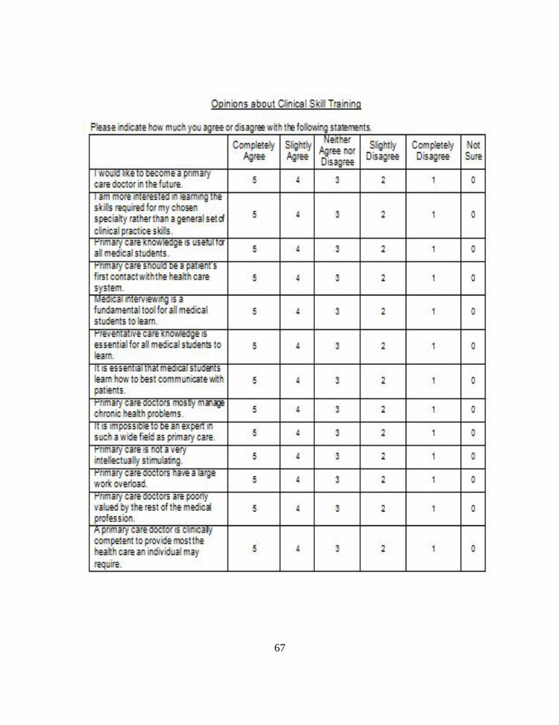
67

APPENDIX B
INSTITUTIONAL REVIEW BOARD EXEMPTION
68

69

APPENDIX C
MANN-WHITNEY U BEGIN MS1 – BEGIN MS2
70

Top Question Variable T1 T3 Sig Trend
How important are the following factors in considering your career in medicine?
• Desire to do primary care 3.04 2.74 .053 Decreasing
• Availability of jobs 3.55 3.86 .013 Increasing
• Opportunity to help patients who are socially disadvantaged 4.17 3.89 .022 Decreasing
• High income potential 2.82 3.36 .000 Increasing
• Status of physicians 2.69 2.97 .073 Increasing
How likely are you to practice medicine in the following underserved populations, specialties, or settings?
• Global Health, via temporary medical missions 3.72 3.28 .003 Decreasing
• Incarcerated/ imprisoned patients 2.39 2.22 .050 Decreasing
• Public health service (Loan payback) 2.85 2.44 .001 Decreasing
• Obstetrics/ gynecology 2.36 1.95 .000 Decreasing
• General surgery 2.91 2.47 .001 Decreasing
• Psychiatry 2.25 1.98 .005 Decreasing
• Emergency Medicine 2.86 3.07 .063 Increasing
How important are the following factors in considering your choice for a specialty?
• Income expectations for the specialty 2.81 3.27 .002 Increasing
• Ability to balance my work life with my family responsibilities 4.37 4.62 .022 Increasing
• The lifestyle of the specialty I am considering 4.20 4.42 .049 Increasing
• Prestige of the specialty I am considering 2.20 2.49 .075 Increasing
Please indicate how much you agree or disagree with the following statements.
• Preventative care knowledge is essential for all medical students to learn
4.83 4.51 .000 Decreasing
• Primary care doctors mostly manage chronic health problems 3.26 3.76 .000 Increasing
• It is impossible to be an expert in such a wide field as primary care 2.69 2.97 .043 Increasing
• Primary care is not very intellectually stimulating 1.90 2.22 .005 Increasing
• Primary care doctors have a large work overload 3.63 3.95 .010 Increasing
• Primary care doctors are poorly valued by the rest of the medical profession
3.48 3.78 .042 Increasing
71

APPENDIX D
MANN-WHITNEY U END MS1 – END MS2
72
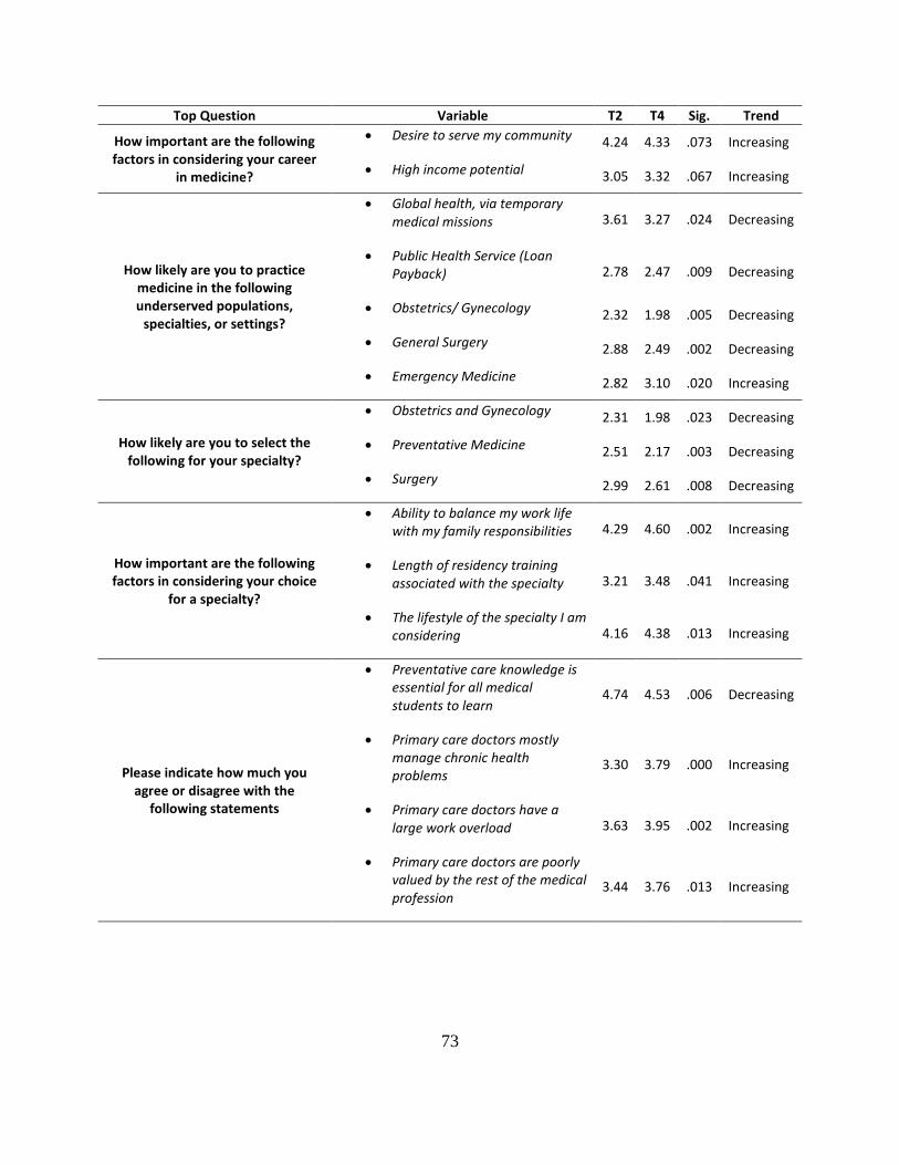
Top Question Variable T2 T4 Sig. Trend
How important are the following factors in considering your career
in medicine?
• Desire to serve my community 4.24 4.33 .073 Increasing
• High income potential 3.05 3.32 .067 Increasing
How likely are you to practice medicine in the following underserved populations,
specialties, or settings?
• Global health, via temporary medical missions 3.61 3.27 .024 Decreasing
• Public Health Service (Loan Payback) 2.78 2.47 .009 Decreasing
• Obstetrics/ Gynecology 2.32 1.98 .005 Decreasing
• General Surgery 2.88 2.49 .002 Decreasing
• Emergency Medicine 2.82 3.10 .020 Increasing
How likely are you to select the following for your specialty?
• Obstetrics and Gynecology 2.31 1.98 .023 Decreasing
• Preventative Medicine 2.51 2.17 .003 Decreasing
• Surgery 2.99 2.61 .008 Decreasing
How important are the following factors in considering your choice
for a specialty?
• Ability to balance my work life with my family responsibilities 4.29 4.60 .002 Increasing
• Length of residency training associated with the specialty 3.21 3.48 .041 Increasing
• The lifestyle of the specialty I am considering 4.16 4.38 .013 Increasing
Please indicate how much you agree or disagree with the
following statements
• Preventative care knowledge is essential for all medical students to learn
4.74 4.53 .006 Decreasing
• Primary care doctors mostly manage chronic health problems
3.30 3.79 .000 Increasing
• Primary care doctors have a large work overload 3.63 3.95 .002 Increasing
• Primary care doctors are poorly valued by the rest of the medical profession
3.44 3.76 .013 Increasing
73

APPENDIX E
MANN-WHITNEY U GENDER COMPARISON
74

Male to Female Significant Changes Top Question Variable Male Female Sig.
How important are the following factors in considering your career in
medicine?
• Opportunity to help patients who are socially disadvantaged 3.81 4.19 .000
• Desire to serve my community 4.27 4.38 .059
• High income potential 3.27 3.00 .011
• Status of physicians 3.00 2.62 .001
How likely are you to practice medicine in the following underserved populations,
specialties, or settings?
• Urban poor, via temporary or part-time free service 3.33 3.66 .000
• Mentally or developmentally disabled, other than as a specialty 2.78 2.98 .014
• Service at a free clinic 3.79 3.99 .003
• Primary care practice (Family, General Peds, Gen Internal) 2.90 3.08 .043
• Obstetrics and Gynecology 1.97 2.33 .000
• General Surgery 2.87 2.45 .000
• Psychiatry 2.01 2.17 .036
• Emergency Medicine 3.21 2.64 .000
How important are the following factors in considering your choice
for a specialty?
• Content of the specialty 4.66 4.74 .016
• Length of residency training associated with the specialty 3.24 3.45 .067
• Opportunities to provide care to underserved populations 3.12 3.49 .001
Please indicate how much you agree or disagree with the following
statements.
• Primary care knowledge is useful for all medical students 4.65 4.73 .051
• Preventative care knowledge is essential for all medical students to learn 4.57 4.74 .002
• A primary care doctor is clinically competent to provide most the health care an individual may require.
3.88 4.05 .017
75

APPENDIX F
IMPORTANT PRINCIPAL COMPONENTS AND T-TESTS FOR BEGIN MS YEAR
76
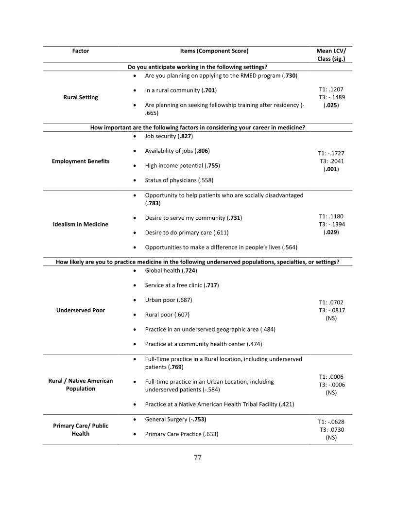
Factor Items (Component Score) Mean LCV/ Class (sig.)
Do you anticipate working in the following settings?
Rural Setting
• Are you planning on applying to the RMED program (.730)
• In a rural community (.701)
• Are planning on seeking fellowship training after residency (-.665)
T1: .1207 T3: -.1489
(.025)
How important are the following factors in considering your career in medicine?
Employment Benefits
• Job security (.827)
• Availability of jobs (.806)
• High income potential (.755)
• Status of physicians (.558)
T1: -.1727 T3: .2041
(.001)
Idealism in Medicine
• Opportunity to help patients who are socially disadvantaged (.783)
• Desire to serve my community (.731)
• Desire to do primary care (.611)
• Opportunities to make a difference in people’s lives (.564)
T1: .1180 T3: -.1394
(.029)
How likely are you to practice medicine in the following underserved populations, specialties, or settings?
Underserved Poor
• Global health (.724)
• Service at a free clinic (.717)
• Urban poor (.687)
• Rural poor (.607)
• Practice in an underserved geographic area (.484)
• Practice at a community health center (.474)
T1: .0702 T3: -.0817
(NS)
Rural / Native American Population
• Full-Time practice in a Rural location, including underserved patients (.769)
• Full-time practice in an Urban Location, including underserved patients (-.584)
• Practice at a Native American Health Tribal Facility (.421)
T1: .0006 T3: -.0006
(NS)
Primary Care/ Public Health
• General Surgery (-.753)
• Primary Care Practice (.633)
T1: -.0628 T3: .0730
(NS)
77
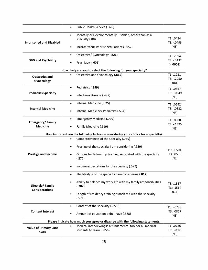
• Public Health Service (.376)
Imprisoned and Disabled
• Mentally or Developmentally Disabled, other than as a specialty (.802)
• Incarcerated/ Imprisoned Patients (.652)
T1: .0424 T3: -.0493
(NS)
OBG and Psychiatry
• Obstetrics/ Gynecology (.826)
• Psychiatry (.606)
T1: .2694 T3: -.3132
(<.0001)
How likely are you to select the following for your specialty?
Obstetrics and Gynecology
• Obstetrics and Gynecology (.815) T1: .1921 T3: -.2950
(.044)
Pediatrics Specialty
• Pediatrics (.899)
• Infectious Disease (.497)
T1: .0357 T3: -.0549
(NS)
Internal Medicine
• Internal Medicine (.875)
• Internal Medicine/ Pediatrics (.534)
T1: .0542 T3: -.0832
(NS)
Emergency/ Family Medicine
• Emergency Medicine (.799)
• Family Medicine (.619)
T1: .0908 T3: -.1395
(NS)
How important are the following factors in considering your choice for a specialty?
Prestige and Income
• Competitiveness of the specialty (.749)
• Prestige of the specialty I am considering (.730)
• Options for fellowship training associated with the specialty (.577)
• Income expectations for the specialty (.572)
T1: -.0501 T3: .0595
(NS)
Lifestyle/ Family Considerations
• The lifestyle of the specialty I am considering (.817)
• Ability to balance my work life with my family responsibilities (.787)
• Length of residency training associated with the specialty (.571)
T1:-.1317 T3: .1564
(.016)
Content Interest
• Content of the specialty (-.770)
• Amount of education debt I have (.588)
T1: -.0738 T3: .0877
(NS)
Please indicate how much you agree or disagree with the following statements.
Value of Primary Care Skills
• Medical interviewing is a fundamental tool for all medical students to learn (.856)
T1: .0726 T3: -.0861
(NS)
78

• It is essential that medical students learn how to best communicate with patients ( .794)
• Preventative care knowledge is essential for all medical students to learn (.698)
• Primary care knowledge is useful for all medical students (.677)
Negative/ Antagonistic View of Primary Care
• Primary care doctors mostly manage chronic health problems (.812)
• It is impossible to be an expert in such a wide field as primary care (.692)
• I am more interested in learning the skills required for my chosen specialty rather than a general set of clinical practice skills. (.532)
T1: -.2077 T3: .2463 (<.0001)
Possible Primary Care Career
• A primary care doctor is clinically competent to provide most the health care an individual may require (.653)
• Primary care should be a patient’s first contact with the health care system (.611)
• I would like to become a primary care doctor in the future (.563)
• Primary care is not very intellectually stimulating (-.532)
T1: .0737 T3: -.0874
(NS)
Negative/ Sympathetic View of Primary Care
• Primary care doctors are poorly valued by the rest of the medical profession (.802)
• Primary care doctors have a large work overload (.770)
T1: -.1517 T3: .1799 (<.0001)
79

APPENDIX G
IMPORTANT PRINCIPAL COMPONENTS AND T-TESTS FOR END MS YEAR
80

Mean LCV/Class (sig.) Do you anticipate working in the following settings?
Rural Setting
• Are you planning on applying to the RMED program (.787)
• In a rural community (.772)
• Are planning on seeking fellowship training after residency (-.624)
T2: .1198 T4: -.1251
(.042)
How important are the following factors in considering your career in medicine?
Idealism and Primary Care
• Desire to serve my community (.756)
• Opportunity to help patients who are socially disadvantaged(.741)
• Desire to do primary care (.702)
T2: .0074 T4: -.0075
(NS)
Status and Income
• Status of physicians (.862)
• High income potential (.771)
T2: -.0735 T4: .0746
(NS)
How likely are you to practice medicine in the following underserved populations, specialties, or settings?
Rural/ Primary Care
• Full-Time Practice in a Rural Location, including underservedpatients (.828)
• Rural Poor (.667)
• Practice in an underserved geographic area (.505)
• Practice at a Native American Health Tribal Facility (.416)
• Primary care practice (.401)
T2: .0021 T4: -.0022
(NS)
Global/ Urban Poor
• Global Health (.748)
• Urban Poor (.701)
• Service at a Free Clinic (.634)
T2: .0354 T4: -.0370
(NS)
Incarcerated and Disabled
• Incarcerated/ Imprisoned Patients (.691)
• Mentally or Developmentally Disabled, other than as aspecialty (.635)
• Full-Time Practice in an Urban Location, includingunderserved patients (.514)
• Public Health Service (.429)
T2: .0742 T4: -.0775
(NS)
OBG/ Psychiatry
• Obstetrics/ Gynecology (.858)
• Psychiatry (.657)
T2: .1566 T4: -.1635
(.007)
81
Factor Items (Component Score)
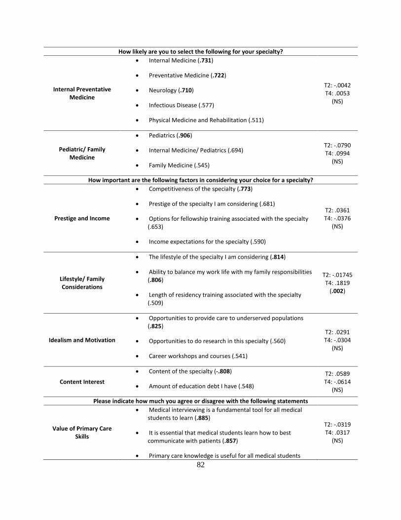
How likely are you to select the following for your specialty?
Internal Preventative Medicine
• Internal Medicine (.731)
• Preventative Medicine (.722)
• Neurology (.710)
• Infectious Disease (.577)
• Physical Medicine and Rehabilitation (.511)
T2: -.0042 T4: .0053
(NS)
Pediatric/ Family Medicine
• Pediatrics (.906)
• Internal Medicine/ Pediatrics (.694)
• Family Medicine (.545)
T2: -.0790 T4: .0994
(NS)
How important are the following factors in considering your choice for a specialty?
Prestige and Income
• Competitiveness of the specialty (.773)
• Prestige of the specialty I am considering (.681)
• Options for fellowship training associated with the specialty (.653)
• Income expectations for the specialty (.590)
T2: .0361 T4: -.0376
(NS)
Lifestyle/ Family Considerations
• The lifestyle of the specialty I am considering (.814)
• Ability to balance my work life with my family responsibilities (.806)
• Length of residency training associated with the specialty (.509)
T2: -.01745 T4: .1819
(.002)
Idealism and Motivation
• Opportunities to provide care to underserved populations (.825)
• Opportunities to do research in this specialty (.560)
• Career workshops and courses (.541)
T2: .0291 T4: -.0304
(NS)
Content Interest
• Content of the specialty (-.808)
• Amount of education debt I have (.548)
T2: .0589 T4: -.0614
(NS)
Please indicate how much you agree or disagree with the following statements
Value of Primary Care Skills
• Medical interviewing is a fundamental tool for all medical students to learn (.885)
• It is essential that medical students learn how to best communicate with patients (.857)
• Primary care knowledge is useful for all medical students
T2: -.0319 T4: .0317
(NS)
82

(.764)
• Preventative care knowledge is essential for all medical students to learn (.653)
Possible Primary Care Career
• I would like to become a primary care doctor in the future (.690)
• Primary care should be a patient’s first contact with the health care system (.633)
• Primary care is not very intellectually stimulating (-.606)
• A primary care doctor is clinically competent to provide most of the health care an individual may require (.549)
T2: .0734 T4: -.0729
(NS)
Negative/ Antagonistic View of Primary Care
• Primary care doctors mostly manage chronic health problems (.781)
• It is impossible to be an expert in such a wide field as primary care (.767)
• I am more interested in learning the skills required for my chosen specialty rather than a general set of clinical practice skills (.403)
T2: -.1823 T4: .1811
(.002)
Negative/ Sympathetic View of Primary Care
• Primary care doctors have a large work overload (.808)
• Primary care doctors are poorly valued by the rest of the medical profession (.785)
T2: -.2051 T4: .2037
(.001)
83
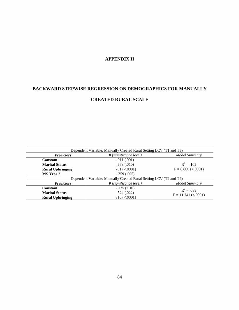
APPENDIX H
BACKWARD STEPWISE REGRESSION ON DEMOGRAPHICS FOR MANUALLY
CREATED RURAL SCALE
Dependent Variable: Manually Created Rural Setting LCV (T1 and T3) Predictors β (significance level) Model Summary
Constant .011 (.901) R2 = .102
F = 8.860 (<.0001) Marital Status .578 (.010) Rural Upbringing .761 (<.0001) MS Year 2 -.359 (.005)
Dependent Variable: Manually Created Rural Setting LCV (T2 and T4) Predictors β (significance level) Model Summary
Constant -.175 (.010) R2 = .089 F = 11.741 (<.0001) Marital Status .524 (.022)
Rural Upbringing .810 (<.0001)
84

APPENDIX I
BACKWARD STEPWISE REGRESSION ON LCV FOR MANUALLY CREATED
RURAL SCALE
Dependent Variable: Manually Created Rural Setting LCV (T1 and T3) Predictors β (significance level) Model Summary
Constant .012 (.854)
R2 = .782 F = 24.279 (<.0001)
Employment Benefits .233 (.007) Underserved Poor .223 (.014) Rural/ Native American Population .795 (<.0001) OBG/ Psychiatry .148 (.021) Pediatric Specialty .152 (.028) Prestige and Income -.162 (.020) Lifestyle/ Family Considerations -.125 (.043) Content Interest -.159 (.058)
Dependent Variable: Manually Created Rural Setting LCV (T2 and T4) Predictors β (significance level) Model Summary
Constant .035 (.503)
R2 = .850 F = 42.211 (<.0001)
Idealism and Primary Care .131 (.029) Rural/ Primary Care .816 (<.0001) Global/ Urban Poor .176 (.001) Incarcerated and Disabled -.086 (.081) OBG/ Psychiatry .103 (.045) Technology Specialty .114 (.046) Prestige and Income -.108 (.058)
85

APPENDIX J
BACKWARD STEPWISE REGRESSION ON COMBINED DEMOGRAPHIC AND LCV
FOR MANUALLY CREATED RURAL SCALE
Dependent Variable: Manually Created Rural Setting LCV (T1 and T3) Predictors β (significance level) Model Summary
Constant -.107 (.220)
R2 = .787 F = 18.900 (<.0001)
Gender .316 (.043) Employment Benefits .248 (.008) Underserved Poor .249 (.011) Rural/ Native American Population .844 (<.0001) OBG/ Psychiatry .127 (.071) Pediatric Specialty .169 (.039) Emergency/ Family Medicine .139 (.095) Lifestyle/ Family Considerations -.175 (.018) Content Interest -.223 (.017)
Dependent Variable: Manually Created Rural Setting LCV (T2 and T4) Predictors β (significance level) Model Summary
Constant -.265 (.003)
R2 = .911 F = 58.705 (<.0001)
Idealism and Primary Care .129 (.009) Rural/ Primary Care .731 (<.0001) Global/ Urban Poor .209 (<.0001) OBG/ Psychiatry .185 (<.0001) Surgery Specialty .085 (.090) Content Interest .124 (.019) White Race .318 (.004) Rural Upbringing .765 (<.0001)
86

BIBLIOGRAPHY
1. Avery, D.M., Jr., et al., Admission factors predicting family medicine specialty choice: a literature review and exploratory study among students in the Rural Medical Scholars Program. J Rural Health, 2012. 28(2): p. 128-36.
2. Rosenblatt, R.A. and L.G. Hart, Physicians and rural America. West J Med, 2000. 173(5): p. 348-51.
3. Rabinowitz, H.K., et al., Medical school programs to increase the rural physician supply: a systematic review and projected impact of widespread replication. Acad Med, 2008. 83(3): p. 235-43.
4. MacDowell, M., et al., A national view of rural health workforce issues in the USA. Rural Remote Health, 2010. 10(3): p. 1531.
5. Dorsey, E.R., D. Jarjoura, and G.W. Rutecki, Influence of controllable lifestyle on recent trends in specialty choice by US medical students. JAMA, 2003. 290(9): p. 1173-8.
6. Rosenthal, M.P., et al., Influence of income, hours worked, and loan repayment on medical students' decision to pursue a primary care career. JAMA, 1994. 271(12): p. 914-7.
7. Institute of Medicine (U.S.). Committee on the Future of Rural Health Care., Quality through collaboration : the future of rural health. 2005, Washington, D.C.: National Academies Press. p. 267.
8. Larson, E.H., et al., Rural health workforce: context, trends and issues. State of the Health Workforce in Rural America: Profiles and Comparisons., 2003: p. 7-14.
9. National Rural Health Association, Access to Health Care for the Uninsured in Rural and Frontier America. 1999.
10. Sundquist, J., M.A. Winkleby, and S. Pudaric, Cardiovascular disease risk factors among older black, Mexican-American, and white women and men: an analysis of NHANES III, 1988-1994. Third National Health and Nutrition Examination Survey. J Am Geriatr Soc, 2001. 49(2): p. 109-16.
11. Barnett, E. and J. Halverson, Local increases in coronary heart disease mortality among blacks and whites in the United States, 1985-1995. Am J Public Health, 2001. 91(9): p. 1499-506.
12. Pearson, T.A. and C. Lewis, Rural epidemiology: insights from a rural population laboratory. Am J Epidemiol, 1998. 148(10): p. 949-57.
13. Eberhardt, M., et al., Urban and Rural Health Chartbook. Health United States, 2001. 14. Zuniga, M., D.A. Anderson, and K. Alexander, Heart disease and stroke in rural
America. Rural Health People 2010, 2003. 1.
87
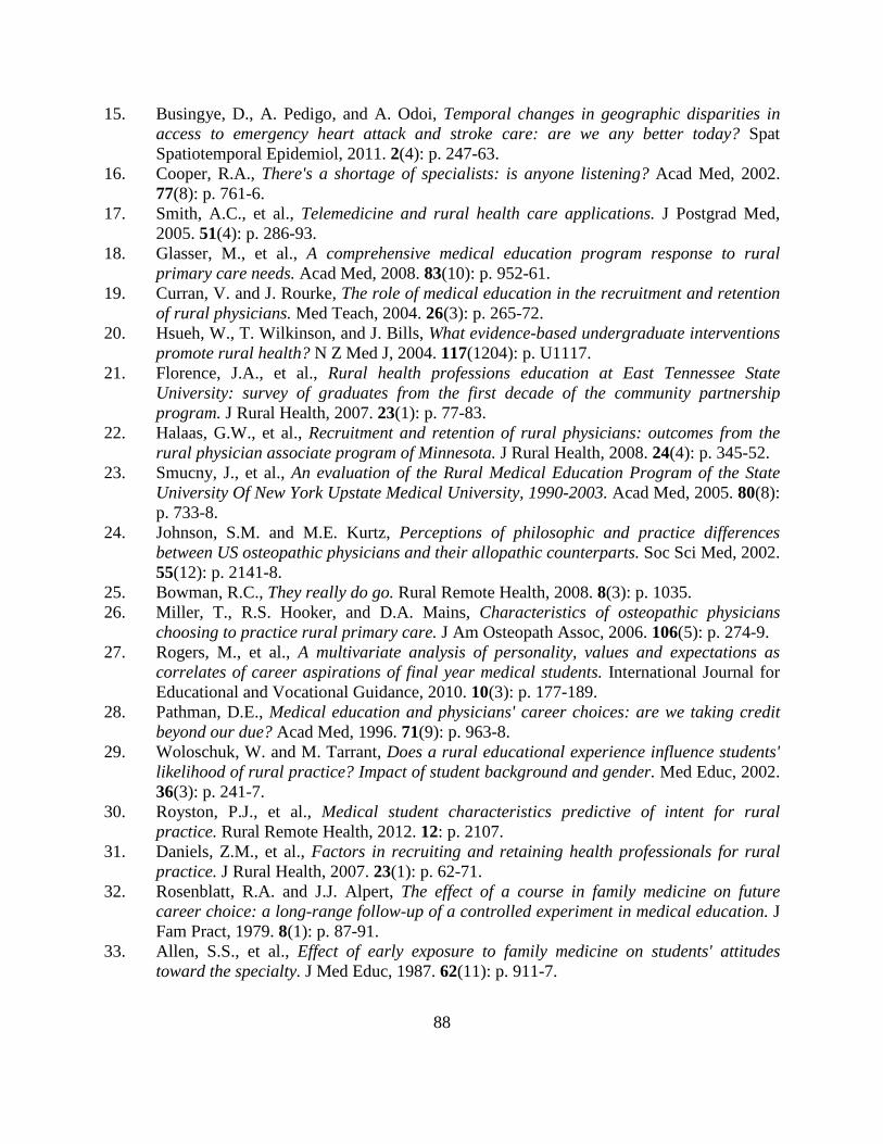
15. Busingye, D., A. Pedigo, and A. Odoi, Temporal changes in geographic disparities in access to emergency heart attack and stroke care: are we any better today? Spat Spatiotemporal Epidemiol, 2011. 2(4): p. 247-63.
16. Cooper, R.A., There's a shortage of specialists: is anyone listening? Acad Med, 2002. 77(8): p. 761-6.
17. Smith, A.C., et al., Telemedicine and rural health care applications. J Postgrad Med, 2005. 51(4): p. 286-93.
18. Glasser, M., et al., A comprehensive medical education program response to rural primary care needs. Acad Med, 2008. 83(10): p. 952-61.
19. Curran, V. and J. Rourke, The role of medical education in the recruitment and retention of rural physicians. Med Teach, 2004. 26(3): p. 265-72.
20. Hsueh, W., T. Wilkinson, and J. Bills, What evidence-based undergraduate interventions promote rural health? N Z Med J, 2004. 117(1204): p. U1117.
21. Florence, J.A., et al., Rural health professions education at East Tennessee State University: survey of graduates from the first decade of the community partnership program. J Rural Health, 2007. 23(1): p. 77-83.
22. Halaas, G.W., et al., Recruitment and retention of rural physicians: outcomes from the rural physician associate program of Minnesota. J Rural Health, 2008. 24(4): p. 345-52.
23. Smucny, J., et al., An evaluation of the Rural Medical Education Program of the State University Of New York Upstate Medical University, 1990-2003. Acad Med, 2005. 80(8): p. 733-8.
24. Johnson, S.M. and M.E. Kurtz, Perceptions of philosophic and practice differences between US osteopathic physicians and their allopathic counterparts. Soc Sci Med, 2002. 55(12): p. 2141-8.
25. Bowman, R.C., They really do go. Rural Remote Health, 2008. 8(3): p. 1035. 26. Miller, T., R.S. Hooker, and D.A. Mains, Characteristics of osteopathic physicians
choosing to practice rural primary care. J Am Osteopath Assoc, 2006. 106(5): p. 274-9. 27. Rogers, M., et al., A multivariate analysis of personality, values and expectations as
correlates of career aspirations of final year medical students. International Journal for Educational and Vocational Guidance, 2010. 10(3): p. 177-189.
28. Pathman, D.E., Medical education and physicians' career choices: are we taking credit beyond our due? Acad Med, 1996. 71(9): p. 963-8.
29. Woloschuk, W. and M. Tarrant, Does a rural educational experience influence students' likelihood of rural practice? Impact of student background and gender. Med Educ, 2002. 36(3): p. 241-7.
30. Royston, P.J., et al., Medical student characteristics predictive of intent for rural practice. Rural Remote Health, 2012. 12: p. 2107.
31. Daniels, Z.M., et al., Factors in recruiting and retaining health professionals for rural practice. J Rural Health, 2007. 23(1): p. 62-71.
32. Rosenblatt, R.A. and J.J. Alpert, The effect of a course in family medicine on future career choice: a long-range follow-up of a controlled experiment in medical education. J Fam Pract, 1979. 8(1): p. 87-91.
33. Allen, S.S., et al., Effect of early exposure to family medicine on students' attitudes toward the specialty. J Med Educ, 1987. 62(11): p. 911-7.
88

34. Beasley, J.W., Does teaching by family physicians in the second year of medical school increase student selection of family practice residencies? Fam Med, 1993. 25(3): p. 174-5.
35. Rezler, A.G. and S.G. Kalishman, Who goes into family medicine? J Fam Pract, 1989. 29(6): p. 652-6.
36. Burkett, G.L. and M.H. Gelula, Characteristics of students preferring family practice/primary care careers. J Fam Pract, 1982. 15(3): p. 505-12.
37. Madison, D.L., Medical school admission and generalist physicians: a study of the class of 1985. Acad Med, 1994. 69(10): p. 825-31.
38. Gorenflo, D.W., M.T.t. Ruffin, and K.J. Sheets, A multivariate model for specialty preference by medical students. J Fam Pract, 1994. 39(6): p. 570-6.
39. Carline, J.D. and T. Greer, Comparing physicians' specialty interests upon entering medical school with their eventual practice specialties. Acad Med, 1991. 66(1): p. 44-6.
40. Harris, D.L., M. Coleman, and M. Mallea, Impact of participation in a family practice track program on student career decisions. J Med Educ, 1982. 57(8): p. 609-14.
41. Glasser, M., A.A. Sarnowski, Jr., and B. Sheth, Career choices from medical school to practice: findings from a regional clinical education site. J Med Educ, 1982. 57(6): p. 442-8.
42. Leonardson, G., R. Lapierre, and D. Hollingsworth, Factors predictive of physician location. J Med Educ, 1985. 60(1): p. 37-43.
43. Colegrove, D.J. and B.E. Whitacre, Interest in rural medicine among osteopathic residents and medical students. Rural Remote Health, 2009. 9(3): p. 1192.
44. Mann-Whitney U, in The Penguin Dictionary of Psychology. 2009, Penguin. 45. Fay, M.P. and M.A. Proschan, Wilcoxon-Mann-Whitney or t-test? On assumptions for
hypothesis tests and multiple interpretations of decision rules. Stat Surv, 2010. 4: p. 1-39. 46. Abdi, H. and L.J. Williams, Principal component analysis. Wiley Interdisciplinary
Reviews: Computational Statistics, 2010. 2(4): p. 433-459. 47. Groth, D., et al., Principal components analysis. Methods Mol Biol, 2013. 930: p. 527-
47. 48. SAGE Publications, I., Principal Components Analysis. Encyclopedia of Research
Design. SAGE Publications, Inc. Thousand Oaks, CA: SAGE Publications, Inc. 49. Weisstein, E.W. Linear Combination. Available from:
http://mathworld.wolfram.com/LinearCombination.html. 50. Orthogonal, in The Penguin Dictionary of Science. 2009, Penguin. 51. Student's t test, in Macmillan Dictionary of Toxicology. 1999, Macmillan Publishers Ltd. 52. Student’s t-test, in Encyclopaedic Dictionary of Psychology. 2006, Routledge. 53. Cronbach's alpha, in The Penguin Dictionary of Psychology. 2009, Penguin. 54. Connelly, L.M., Cronbach's Alpha, in MedSurg Nursing2011. p. 45+. 55. Ordinary Least Squares Regression, in International Encyclopedia of the Social Sciences,
W.A. Darity, Jr., Editor. 2008, Macmillan Reference USA: Detroit. p. 57-61. 56. Laurent, R.T.S., Review of Understanding Regression Assumptions by W.D. Berry.
Technometrics, 1994. 36(3): p. 321. 57. Regression Diagnostics. Introduction to SAS; Available from:
http://www.ats.ucla.edu/stat/spss/webbooks/reg/chapter2/spssreg2.htm.
89
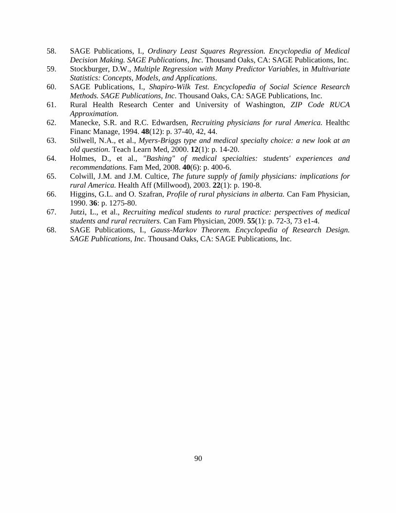
58. SAGE Publications, I., Ordinary Least Squares Regression. Encyclopedia of Medical Decision Making. SAGE Publications, Inc. Thousand Oaks, CA: SAGE Publications, Inc.
59. Stockburger, D.W., Multiple Regression with Many Predictor Variables, in Multivariate Statistics: Concepts, Models, and Applications.
60. SAGE Publications, I., Shapiro-Wilk Test. Encyclopedia of Social Science Research Methods. SAGE Publications, Inc. Thousand Oaks, CA: SAGE Publications, Inc.
61. Rural Health Research Center and University of Washington, ZIP Code RUCA Approximation.
62. Manecke, S.R. and R.C. Edwardsen, Recruiting physicians for rural America. Healthc Financ Manage, 1994. 48(12): p. 37-40, 42, 44.
63. Stilwell, N.A., et al., Myers-Briggs type and medical specialty choice: a new look at an old question. Teach Learn Med, 2000. 12(1): p. 14-20.
64. Holmes, D., et al., "Bashing" of medical specialties: students' experiences and recommendations. Fam Med, 2008. 40(6): p. 400-6.
65. Colwill, J.M. and J.M. Cultice, The future supply of family physicians: implications for rural America. Health Aff (Millwood), 2003. 22(1): p. 190-8.
66. Higgins, G.L. and O. Szafran, Profile of rural physicians in alberta. Can Fam Physician, 1990. 36: p. 1275-80.
67. Jutzi, L., et al., Recruiting medical students to rural practice: perspectives of medical students and rural recruiters. Can Fam Physician, 2009. 55(1): p. 72-3, 73 e1-4.
68. SAGE Publications, I., Gauss-Markov Theorem. Encyclopedia of Research Design. SAGE Publications, Inc. Thousand Oaks, CA: SAGE Publications, Inc.
90