Embed Size (px)
Citation preview

Mechanistic Studies of
Liquid Metal Electrode
Solid Oxide Fuel Cells
Aliya Toleuova
A thesis submitted to University College London
for the degree of Doctor of Philosophy
September 2015
Department of Chemical Engineering
Torrington Place, London, WC1E 7JE

Declaration
I, Aliya Toleuova, confirm that the work presented in this thesis is my own. Where
information has been derived from other sources, I confirm that this has been indicated in
the thesis.
_______________________
Signature
September 2015

Dedicated to my parents, my sister and my loving husband,
who have always believed in me.

Acknowledgements
iv
Acknowledgements Firstly, I would like to thank my supervisor – Dr. Dan Brett for giving me the opportunity
to study at UCL and do my PhD. I had a great pleasure working with you, your constant
belief in me and support throughout my studies was the driving force for the
accomplishment of my research goals. Thanks for your encouragement and kindness not
only in my studies, but also in my personal life. I would also like to thank my secondary
supervisor – Dr. Paul Shearing for his supervision and guidance, particularly for useful
comments during my Transfer Viva that helped me to set the rest of my work.
Secondly, I would like to express my deepest gratitude to the visiting academic at UCL -
Dr. Bill Maskell, who is a true inspiration for me. I am so grateful that you have joined this
project when I started and have led me through my research journey. My transformation
from a chemical technologist to an electrochemical engineer could not be possible without
your constant guidance, assistance and valuable experience. I am very thankful for your
assistance in development of the electrochemical model and discussion of experimental
results, as well as ideas on the Rotating Electrolyte Disc technique. Thank you for all your
help.
My sincere thanks go to Dr. Vladimir Yufit for his help and assistance especially at early
stages of this project, for constructive and critical view on the work in general and valuable
comments on the papers.
Thanks to my sponsor “Center for International Programs”, Government of Republic of
Kazakhstan and Nazarbayev University for awarding me BOLASHAK International
Scholarship that covered full expenses at UCL.
I especially thank Graeme Smith and Erich Herrmann in the Workshop, Albert Corredera
in Electronics Department for their professional help, Mike Gorecki and Simon Barrass for
assistance with technical and safety aspects in the lab and the office. Thanks to Mae, Agata,
Katy and Claire for processing of administrative jobs. I would like to thank all my PhD
colleagues and postdocs at the Electrochemical Innovation Lab for their help and general
support in the lab, particularly to Mithila, Jason, Toby, Tom and Ishanka. Special thanks to
my office neighbours Amal, Lawrence, Mayowa, Quentin, Phil, Rhod and Chaoran for all
the lovely moments we had together. I would also like to thank my friends in London –
Assiya and Saule for wonderful time spent outside UCL, for sightseeing of London, for
inspirational talks and discussions and many more. Thanks to all my friends back in
Kazakhstan, in particular to Gulsamal who has encouraged and supported me throughout.
Finally, and above all, I would like to thank my parents, my sister for their love, support
and prayers. Thank you for insisting on doing this PhD degree and encouraging me to
believe in my dream, to be hard-working, persistent and strong in any situation. I cannot
express my unfailing love and gratitude to my loving husband. I am so grateful that I met
you during my PhD; my life without you would not be complete. Thank you for believing
in me!

Abstract
v
Abstract Liquid metal electrode solid oxide fuel cells (LME SOFC) offer the advantage of high
efficiency with the benefits of multi-fuel operation, the concept being particularly well-
suited to the direct use of solid fuel. With respect to reported uncertainties in performance
limitations of SOFCs with liquid metal anodes (LMA), in-depth understanding of the fuel
oxidation mechanisms and transport processes within liquid metal electrodes is needed.
This study provides improved understanding of the operation of LME SOFCs using novel
experimental and modelling approaches. H2 oxidation in LMA SOFC in a specific potential
range was chosen as the model system. A classification setting out four possible
mechanisms of oxidation of H2 is proposed. Two models are developed based upon
Electrochemical (E) and Chemical-Electrochemical (CE) modes of operation of H2-LMA
SOFC under conditions that eliminate the detrimental effects of metal oxide layer
formation at the electrolyte-electrode interface.
The E mode model of operation was found to be inconsistent with literature knowledge of
H2 solubility in liquid tin. A possible explanation considered is the generation of metallic
foam effectively ‘storing’ hydrogen within its matrix, but this was not observed
experimentally. Thus mode E (direct anodic oxidation of hydrogen in LMA SOFC) is not
applicable to this system.
A major contribution of this work is the development and validation of a model for the
CE mode. This is based upon fast dissolution of hydrogen in a molten tin anode, rate-
determining homogeneous reaction of hydrogen with oxygen dissolved in the liquid tin,
followed by anodic oxygen injection under diffusion control to replace the oxygen
removed by chemical reaction. A new key parameter, related to the Damkohler number,
termed the dynamic oxygen utilisation coefficient, (𝑧 ), evolved out of the model; its value
is determined by geometric, mass-transport and kinetic factors in the cell, as well as the
partial pressure of the supplied hydrogen fuel. Current output of the cell is proportional to
the value of 𝑧 . This parameter is expected to have important implications regarding the
design, development and commercialisation of the technology.
Additional validation of the CE mode model included development and application of a
method named anodic injection coulometry (with similarities to anodic stripping
voltammetry) for determination of the parameter 𝑧 , as well as measurement of the oxygen
solubility in liquid tin. Feeding H2 at 16 kPa partial pressure into the LME SOFC resulted
in a 𝑧 value of 0.83 under the chosen conditions. This is consistent with a separate

Abstract
vi
estimate in this study using an unrelated method. The solubility of oxygen at 780 °C was
found to be 0.10 at.%, which is comparable to literature values.
The possibility of application of the liquid metal electrode/ YSZ system for water
electrolysis in solid oxide electrolysers (SOE) is explored. An electrochemical model is
presented for interpretation of generated experimental results.
Application of a glassy carbon rod as a low-cost current collector dipping into the liquid tin
electrode was successfully pioneered in this work; it showed stable operation without
corrosion throughout the whole project at the chosen operating temperature of 780 °C.
A novel rotating electrolyte disc (RED) apparatus is proposed, which is an inverted
arrangement of the well-known rotating disc electrode (RDE). The RED offers the
prospect of measuring transport properties of active species within a liquid metal electrode.
Initial studies towards the development of this technique have been undertaken.

List of Publications
vii
List of Publications Peer-reviewed journal papers:
1. A. Toleuova, V. Yufit, S. Simons, W. C. Maskell, and D. J. L. Brett, “A Review of
Liquid Metal Electrode Solid Oxide Fuel Cells”, J. Electrochem. Sci. Eng, 3, 91–105
(2013).
2. A. Toleuova, W. C. Maskell, V. Yufit, P. R. Shearing, and D. J. Brett, “Mechanistic
Studies of Liquid Metal Anode SOFCs I. Oxidation of Hydrogen in Chemical -
Electrochemical Mode”, J. Electrochem. Soc., 162, F988–F999 (2015).
3. A. Toleuova, W. C. Maskell, V. Yufit, P. R. Shearing, and D. J. Brett , “Mechanistic
Studies of Liquid Metal Anode SOFCs II. Validation of Chemical-Electrochemical
Mechanism and Determination of Oxygen Solubility using Anodic Injection
Coulometry” (submitted for publication).
Peer-reviewed conference papers:
1. A. Toleuova, V. Yufit, S. J. R. Simons, W. C. Maskell, and D. J. L. Brett, “Rotating
Electrolyte Disc (RED) for Operation in Liquid Metal Anode SOFCs”, ECS Trans.,
58, 65 (2013).
2. A. Toleuova, W. C. Maskell, V. Yufit, P. R. Shearing, and D. J. Brett “Mechanistic
Considerations of Liquid Metal Anode SOFCs Fuelled with Hydrogen”, ECS
Trans., XX, XX (2015) (accepted for publication).
Presentations:
1. 6th European Summer School on Electrochemical Engineering (2012), Zagreb,
Croatia – Poster: “Studies Relating to Solid Oxide Fuel Cells with Liquid Metal
Electrodes”.
2. 224th Electrochemical Society Meeting, (2013), San Francisco, USA - Presentation:
“A Rotating Electrolyte Disc (RED) for Operation in Liquid Metal Anode
SOFCs”.
3. H2FC Supergen conference (2013), Birmingham, UK, Poster: “A Rotating
Electrolyte Disc for Operation in Liquid Metal Anode SOFCs”.
4. ECS Conference on Electrochemical Conversion and Storage with SOFC-XIV
(2015), Glasgow, UK, Presentation: “Mechanistic Considerations of Liquid Metal
Anode SOFCs Fuelled with Hydrogen”.

Table of Contents
viii
Table of Contents Declaration ............................................................................................................. ii Acknowledgements ................................................................................................ iv Abstract .................................................................................................................... v List of Publications ............................................................................................... vii Table of Contents ................................................................................................. viii List of Tables ........................................................................................................... x List of Figures ........................................................................................................ xi
1. Introduction ..................................................................................................... 1 1.1. Research Aims .............................................................................................................. 3 1.2. Thesis outline ............................................................................................................... 3
2. Literature Review ............................................................................................. 6 2.1. Fuel Cells....................................................................................................................... 7 2.2. Solid Oxide Fuel Cells............................................................................................... 10 2.3. Liquid Metal Electrode Electrochemical Systems ................................................ 25 2.4. Conclusions ................................................................................................................ 45
3. Experimental methods and equipment ......................................................... 46 3.1. Experimental workstation ........................................................................................ 47 3.2. Electrochemical cell .................................................................................................. 50 3.3. Methodology .............................................................................................................. 55 3.4. Experimental Methods: electrochemical techniques ............................................ 56 3.5. Conclusions ................................................................................................................ 60
4. Preliminary testing ......................................................................................... 62 4.1. Introduction ............................................................................................................... 63 4.2. Background................................................................................................................. 63 4.3. Experimental procedure ........................................................................................... 65 4.4. Results and discussion .............................................................................................. 65 4.5. Conclusions ................................................................................................................ 72
5. Experimental optimisation ............................................................................ 74 5.1. Introduction ............................................................................................................... 75 5.2. Background................................................................................................................. 75 5.3. Experimental procedure ........................................................................................... 78 5.4. Results and discussion .............................................................................................. 82 5.5. Conclusion .................................................................................................................. 89
6. Proposed mechanisms for oxidation of hydrogen in LMA SOFCs ............... 91 6.1. Introduction ............................................................................................................... 92 6.2. Classification of modes of operation for H2-LMA SOFCs ................................. 93 6.3. Thermodynamics of the modes of operation for LMA SOFCs ......................... 95 6.4. Experimental procedure ........................................................................................... 96 6.5. Oxidation of hydrogen in LTA SOFC operated in mode EC1/EC2 ............... 96 6.6. Conclusions ................................................................................................................ 98

Table of Contents
ix
7. Oxidation of hydrogen in LTA SOFC in mode E/CE .................................. 99 7.1. Introduction ............................................................................................................. 100 7.2. Experimental procedure ......................................................................................... 100 7.3. Oxidation of hydrogen in LTA SOFCs in mode E/CE ................................... 101 7.4. Electrochemical model for E mode ..................................................................... 104 7.5. Investigation of a possibility of a metal foam in LTA SOFC ........................... 109 7.6. Electrochemical model for CE mode ................................................................... 120 7.7. Conclusion ................................................................................................................ 134
8. Additional validation of CE model ...............................................................135 8.1. Introduction ............................................................................................................. 136 8.2. Background literature concerning oxygen and hydrogen solubilities .............. 136 8.3. Experimental procedure ......................................................................................... 138 8.4. Results and discussion ............................................................................................ 138 8.5. Conclusion ................................................................................................................ 147
9. Water electrolysis in reverse LME SOFCs ....................................................148 9.1. Introduction ............................................................................................................. 149 9.2. Experimental procedure ......................................................................................... 149 9.3. Results and discussion ............................................................................................ 151 9.4. Conclusion ................................................................................................................ 159
10. Rotating Electrolyte Disc system design and testing ................................... 161 10.1. Introduction ............................................................................................................. 162 10.2. Development of the RED set-up .......................................................................... 164 10.3. The RED modified for aqueous electrochemical systems ................................ 167 10.4. Application of RED to LME SOFCs ................................................................... 174 10.5. Conclusion ................................................................................................................ 178
11. Conclusion and future work ..........................................................................180 11.1. Conclusion ................................................................................................................ 180 11.2. Recommendations for future work ....................................................................... 184
Nomenclature .......................................................................................................188
References ............................................................................................................193
Appendix ............................................................................................................. 203 A. Electrical furnace temperature profile ......................................................... 203 B. Determination of permeability coefficient for plastic tubing ...................... 204 C. Electrochemical model for Anodic Oxidation of Hydrogen in Electrochemical mode ........................................................................................ 206
Model 1 .................................................................................................................................. 206 Model 2 .................................................................................................................................. 208 Additional Mechanistic Theory .......................................................................................... 210 Determination of the apparent solubility of H2 in liquid tin and the parameter w’ using anodic stripping voltammetry ............................................................................................. 211

List of Tables
x
List of Tables Table 2.1 Technical characteristics of five main fuel cell types25–27............................................ 9
Table 2.2 Common metals properties and abundances, prices (adapted from Abernathy et
al.6). .................................................................................................................................................... 34
Table 2.3 Thermophysical properties of tin6. .............................................................................. 34
Table 2.4 Solubility of oxygen in liquid tin79 . ............................................................................. 35
Table 3.1 Description of the parts a fuel cell. ............................................................................. 54
Table 4.1 Ohmic resistance values for 6 mol. % YSZ symmetrical cell (Pt electrode area of
1.30 cm2) with temperature. ........................................................................................................... 70
Table 4.2 Conductivity values of YSZ electrolytes measured and given in the literature. ... 71
Table 5.1 Details of all the tubing employed in experimental work. ....................................... 80
Table 5.2Permeability in polymers at 25 °C for oxygen gas128. ............................................... 89
Table 7.1 Reciprocal time constants for various p2’ values. .................................................... 125
Table 8.1 Q1 values obtained from with 16 kPa p(H2) for Regime 1 operation. ................... 142
Table 8.2. Q2 values obtained with 16 kPa p(H2) for Regime 2 operation. ........................... 144
Table 9.1 Saturated water vapour pressure at set temperature values from standard tables.
.......................................................................................................................................................... 151
Table 9.2 Q1 values obtained from with 3.8 kPa p(H2O) for Regime 1 operation. .............. 153
Table 9.3. Reciprocal time constants for various destination p(H2O) values. ....................... 158
Table 10.1 Comparison of diffusion coefficients for Fe2+ and Fe3+ ions with literature. ... 174

List of Figures
xi
List of Figures Figure 2.1 Individual fuel cell (one example of polymer electrolyte fuel cell). ......................... 7
Figure 2.2 Flow of ions through different fuel cells electrolyte types. ...................................... 8
Figure 2.3 Schematic view of SOFC operation using hydrogen as a fuel. .............................. 11
Figure 2.4 Schematic of a typical current – voltage or polarisation curve that shows the
operating cell voltage with activation, ohmic and concentration potential losses. ................ 13
Figure 2.5 Schematic view of tubular SOFC28. ........................................................................... 16
Figure 2.6 A schematic of cell-to cell connections in a cathode-supported tubular SOFC
stack24. ............................................................................................................................................... 16
Figure 2.7 Schematic of cell configuration in an anode-supported planar SOFC stack24..... 17
Figure 2.8 Schematic view of planar SOFC28. ............................................................................. 17
Figure 2.9 A schematic of the ‘segmented-in-series’ design adopted by Rolls-Royce24. ....... 17
Figure 2.10 Schematic view of monolith-type SOFC33. ............................................................. 18
Figure 2.11 Conductivity of yttria- and scandia-stabilised zirconia in air at 1000 °C40. ........ 21
Figure 2.12 An idealised Nyquist plot of a zirconia electrochemical cell with electrodes and
its equivalent circuit. The three semi-circular arcs correspond to conductivity within the
grain, grain boundaries and electrodes, respectively47. ............................................................... 22
Figure 2.13 a)LLNL DCFC configuration with carbon particle anode, b) performance of
LLNL DCFC4. ................................................................................................................................. 24
Figure 2.14 Configuration of the SRI direct carbon fuel cell (a), performance of SRI direct
carbon fuel cell (b)4. ........................................................................................................................ 25
Figure 2.15 Operation of liquid metal electrode reactor in fuel cell and electrolyser mode. 25
Figure 2.16 Schematic of solid oxide membrane electrolyser for waste to hydrogen and
syngas conversion53. ........................................................................................................................ 27
Figure 2.17 Schematic showing operation of LMA SOFC with (a) hydrogen and (b) solid
carbon, as the fuel. .......................................................................................................................... 28
Figure 2.18 Effect of temperature on standard equilibrium cell potentials for various metal
oxidation reactions. ......................................................................................................................... 30
Figure 2.19 Ideal Nernst potentials for LTA SOFC for all three reactions62. ........................ 32
Figure 2.20 Sn-O phase diagram determined at 1 bar81. ............................................................ 36
Figure 2.21 Sn-O system phase diagram calculated at 1 bar6. ................................................... 37
Figure 2.22 Power curves for tin based cells operating on hydrogen and JP-8 (a); durability
test on JP-8 (V, W) (b)17. ................................................................................................................ 39
List of Figures
xii
Figure 2.23 (a) Schematic of a LMA SOFC coupled to an external combustion reactor, (b)
Schematic of a LMA Solid Oxide Electrolyser (SOE) coupled to an external combustion
reactor70. ............................................................................................................................................ 40
Figure 2.24 (a) Schematic of liquid copper anode SOFC, (b) polarisation and power density
curves for liquid copper anode SOFC60. ...................................................................................... 42
Figure 3.1 Experimental workstation. .......................................................................................... 48
Figure 3.2 Schematic of experimental rig used for fuel cell testing. ........................................ 49
Figure 3.3 Symmetrical cell: (a) 120 mm long 10YSZ cell for potentiometric measurements;
(b) 6YSZ symmetrical cell for EIS measurements (front view) and side view (c). ................ 50
Figure 3.4 The 3D design of the fuel cell (a): closed end YSZ tube with fuel inlet, exhaust
and current collector and pyrophyllite holder (b). ...................................................................... 51
Figure 3.5 Updated fuel cell design with YSZ thermocouple placed parallel to the vessel. . 52
Figure 3.6 Schematic of a fuel cell used for electrochemical characterisation of LMA SOFC
(held in furnace). .............................................................................................................................. 55
Figure 3.7 Hydrodynamics profile of a rotating disc: (a) streamlines in solution; (b)
coordinate system used in calculation (solid arrows denote the streamlines)108. .................... 59
Figure 4.1 Schematic of experimental rig used for oxygen sensor testing. ............................. 65
Figure 4.2 Schematic of experimental setup for potentiometric measurements (a) with
10YSZ symmetrical cell (b). ........................................................................................................... 66
Figure 4.3 Theoretical (using Equation (4.4)) and experimental EMF developed by the
symmetrical cell. .............................................................................................................................. 67
Figure 4.4 Current – voltage characteristics that includes ionic conductivity of 10YSZ and
overpotential on each Pt electrodes. ............................................................................................. 68
Figure 4.5 Measured EIS data: at 315 - 422 °C frequency sweep: 10 kHz to 0.01Hz, 10
frequencies per decade, Voltage: 0 V, amplitude of oscillations: 10 mV. ............................... 69
Figure 4.6 Measured EIS data at 722, 890 and 1000 °C, frequency sweep: 10 kHz to
0.01Hz, 10 frequencies per decade, Voltage: 0 V, amplitude of oscillations: 10 mV. ........... 69
Figure 4.7 The electrical conductivity of 6 mol. % YSZ cell as a function of reciprocal
absolute temperature. ...................................................................................................................... 70
Figure 4.8 Experimental open circuit potential of the SOFC with a liquid tin anode
compared to the theoretical equilibrium potentials for tin oxidation reaction. ..................... 72
Figure 5.1 Schematic of the oxygen permeation through silicone peroxide tubing
(containing N2) with electrochemically pumped oxygen. .......................................................... 77
Figure 5.2 Electrical furnace for heating oxygen sensor and oxygen pump (closer look) in
the overall set-up (a); oxygen sensor (b); oxygen pump (10YSZ symmetrical cell (closed at
one end) with two Pt electrodes and Pt wires) (c). ..................................................................... 79
List of Figures
xiii
Figure 5.3 Electronic circuit with 10YSZ cell served to pump oxygen in and out of nitrogen
flow (a); schematic of the operation of the oxygen pump using the electronic circuit (b). .. 80
Figure 5.4 Process flow diagram for oxygen permeation and oxygen pumping into the
nitrogen stream (a); schematic of experimental rig for the measurement of oxygen
permeation and oxygen pumping in and/or out the nitrogen flow (expanded view) (b);
schematic of an experimental setup of the LMA SOFC cell for oxygen permeation into the
N2 stream (c). ................................................................................................................................... 81
Figure 5.5 Concentration of oxygen diffused through silicone peroxide tubing of 88 and 8
cm and nylon tubing (8 cm) vs. inverse of the gas flow rate. ................................................... 82
Figure 5.6 Concentration of O2 vs. pumped current with N2 flow rate of 1.67, 0.83 and 0.33
ml s-1 using 8 cm silicone peroxide tubing (a) and hard tubing (b). ......................................... 83
Figure 5.7 Intercepts obtained from Figure 5.6 against reciprocal of the flow rate for
silicone peroxide and nylon tubing. .............................................................................................. 84
Figure 5.8 Relationship between theoretical and measured injection rate of oxygen and gas
flow rate with both silicone peroxide and nylon tubing. ........................................................... 85
Figure 5.9 The effect of pumped in and pumped out current on cathodic current measured
at -1.1 V vs. RE under flow of 1.6 ml s-1 of gaseous mixture of dry H2 and N2 (4: 96). ...... 86
Figure 5.10 Steady cathodic current (a) vs. pumped current and (b) vs. O2 concentration
with total flow rate of 1.6 ml s-1. ................................................................................................... 87
Figure 5.11 Concentration of O2 vs. pumped current at total flow rate of 1.6 ml s-1. .......... 87
Figure 6.1 Schematic showing operation of LMA SOFC with hydrogen. Yttria-stabilised
zirconia (YSZ) is shown as a representative solid oxide electrolyte. ....................................... 92
Figure 6.2. Proposed modes of operation for a LMA SOFC fuelled with H2: (a) direct
electrochemical oxidation of H2 at LMA / electrolyte interface; (b) chemical oxidation of
H2 in the bulk of LMA by dissolved oxygen, followed by electrochemical injection of
oxygen at LMA / electrolyte interface; (c) electrochemical oxidation of M followed by
chemical oxidation of H2 in the bulk of the LMA; (d) extensive oxidation of M to insoluble
MOx that may create a blocking layer. ......................................................................................... 93
Figure 6.3. Standard equilibrium potentials of H2-H2O, Sn-SnO and Sn-SnO2 redox
systems (all based upon O2 at 1 atmosphere pressure and 21% concentration) as functions
of temperature. Operating potential window in E mode (applied in the present work) is
constrained by the onset of electronic conductivity in YSZ from the top and by SnO2
generation from the bottom at 780 °C......................................................................................... 95
Figure 6.4. The effect of applied potential on current density in LTA SOFC in modes EC1
and EC2 with subsequent formation of a blocking layer (SnO2) at 760 °C. ......................... 97

List of Figures
xiv
Figure 7.1. Anodic current at -0.90 V vs. RE at 780 °C (immediately after switching from
3% to zero H2). .............................................................................................................................. 102
Figure 7.2. Anodic current at -0.90 V vs. RE at 780 °C with increase of p(H2) from 0 to 26
kPa (a); and with decrease of p(H2) from 26 kPa to 0 (b). ...................................................... 102
Figure 7.3. Anodic current with variation of p(H2) and of total flow rate (TF) at 780 °C. 103
Figure 7.4. Steady anodic oxidation current as function of p(H2) with varying TF and
direction of change of H2 composition (ascending / descending), all at 780 C. ................ 103
Figure 7.5. Schematic of the step change in p(H2) during oxidation at applied potential in
the E/CE mode of operation. .................................................................................................... 105
Figure 7.6 Electronic circuit with a 741 operational amplifier and a reversing switch for
supply of current of both polarities (100 µA and -100 μA). ................................................... 112
Figure 7.7 Gas tight pyrophyllite holder with O-ring that enabled free movement of GC
rod. .................................................................................................................................................. 113
Figure 7.8 Apparatus for electrical resistance measurements: closer look of pyrophyllite
holder with O-ring and moveable GC rod sheathed in alumina tube (a); complete cell with
8YSZ tube filled with tin shots, alumina inlet and outlet tubes, stationary and moveable GC
rod sheathed in alumina tube (b). ............................................................................................... 114
Figure 7.9 Experimental cell for visualisation of the metal foam consisted of silica tube
(filled with tin shots), alumina inlet and outlet tubes (a); identical s tube (filled with tin shots
and 8YSZ chips), alumina inlet and outlet tubes during the operation at 300 °C (b). ........ 115
Figure 7.10 Process flow diagram for observation of metal foam during the oxidation of
hydrogen in LMA SOFC (foam shown subsequently found not to be present). ................ 116
Figure 7.11 Resistance measured between two probes inside molten tin at 300 °C (at no gas
bubbling) and at 800 °C after gas bubbling as a function of height of liquid tin: using
unsheathed GC probe (a) and using sheathed GC robe (b). .................................................. 117
Figure 7.12 Silica tube apparatus in-operando with no metallic foam above tin: with inlet and
outlet tubes (a) and with added 8YSZ chips (b). ...................................................................... 118
Figure 7.13 Schematic of the dissolved oxygen concentration profile at a given applied
potential in the CE mode of operation. The diffusion layer thickness is shown as δ......... 121
Figure 7.14. Step change in hydrogen partial pressure: from 0 to 8 kPa (total flow rate 2.6
ml s-1) (a); from 8 to 15 kPa (total flow rate 2.8 ml s-1) (b). ..................................................... 126
Figure 7.15. Step change in hydrogen partial pressure: from 15 to 26 kPa (total flow rate 3.2
ml s-1) (a); from 26 to 15 kPa (total flow rate 2.8 ml s-1) (b). ................................................... 126
Figure 7.16. Step change in hydrogen partial pressure: from 15 to 8 kPa (total flow rate 2.6
ml s-1) (a); from 8 kPa to 0 (total flow rate 2.3 ml s-1) (b). ....................................................... 126
List of Figures
xv
Figure 7.17. The reciprocal time constant versus p2’. ............................................................... 127
Figure 7.18. Determined values of R2 and intercept for the plots of i2 versus 𝒛𝟐𝒑𝟐′ versus
𝑲 for a range of values. ................................................................................................................ 129
Figure 7.19 Determined values for the slope of plots of i2 versus 𝒛𝟐𝒑𝟐′ plotted as a
function of 𝑲. ............................................................................................................................... 129
Figure 7.20. The ‘refined’ plot: steady anodic current versus 𝒑𝟐′. Compare Figure 7.4. ... 130
Figure 7.21. Anodic current versus time in LTA SOFC at 780 °C with instantaneous step
change of p(H2) from 0 to 10 kPa, then to back to zero, repeated with 20 kPa and 30 kPa.
.......................................................................................................................................................... 132
Figure 7.22. Current-time curves after switching the hydrogen partial pressure from 0 to 10
kPa (a); 20 kPa (b); 30 kPa(c). Slopes of the lines in (a-c) vs. p(H2) are shown in (d)......... 133
Figure 8.1 Reported solubility of oxygen in liquid tin. ............................................................ 137
Figure 8.2 Schematic representation of Regime 1 conditions applied to the working cell:
same hydrogen partial pressure, p’2 is applied from A to D; potential is held at a value E
everywhere except in B - C. ......................................................................................................... 139
Figure 8.3 Operation of the working cell under Regime 1 with 16 kPa p(H2) at 780 °C. ... 141
Figure 8.4. Schematic representation of Regime 2 conditions applied to the working cell
flushed with constant flow of argon. .......................................................................................... 142
Figure 8.5 Operation of the working cell under Regime 2 with 16 kPa p(H2) at 780 °C. ... 143
Figure 8.6 Schematic representation of Regime 3 conditions applied to the working cell
flushed with constant flow of argon; potential is held at a value E everywhere except in B -
C. ...................................................................................................................................................... 144
Figure 9.1 Process flow diagram for dissociation of water in LMA SOFC cell followed by
cathodic reduction of oxygen (with optional use of H2 for additional removal of tin oxide).
.......................................................................................................................................................... 151
Figure 9.2 Cathodic current at -1.1 V vs. RE at 810 °C with changes of p(H2O). .............. 152
Figure 9.3 Steady cathodic current data as a function of p(H2O) corrected for parasitic
oxygen current. .............................................................................................................................. 152
Figure 9.4 Operation of LTA SOFC under Regime 1 with constant 3.8 kPa p(H2O). ....... 153
Figure 9.5 Measured Q1 values as a function of OC intervals. ............................................... 154
Figure 9.6 Schematic of the dissolved oxygen concentration profile at a given applied
potential E during the water reduction process. The diffusion layer thickness is shown as δ.
(Compare with Figure 7.13). ........................................................................................................ 155
Figure 9.7 Step change in p(H2O): from 3.78(28 °C) to 0.61(0 °C) kPa (a); from 0.61kPa (0
°C) to zero (dry Ar) (b). ................................................................................................................ 158

List of Figures
xvi
Figure 9.8 Step change in p(H2O): from zero (dry Ar) to 1.23 kPa (10 °C) (a); from 3.78 kPa
(28 °C) to 1.23 kPa (10 °C) (b). ................................................................................................... 158
Figure 10.1 (a) Schematic of a rotating disc electrode of the classical Riddiford design
where the electrode is a platinum wire of 1 to 3 mm radius168; (b) schematic of rotating
ring-disc electrode171 (the broken arrow indicates the electrolyte-flow lines induced by
rotation). ......................................................................................................................................... 163
Figure 10.2 Initial schematic of the cell containing Rotating Electrolyte Disc (Design 1). 166
Figure 10.3 The improved design of RED - Design 2. ........................................................... 167
Figure 10.4 Design for simplified RED setup in aqueous systems. ....................................... 168
Figure 10.5 The outer side of YSZ disc painted with Pt ink (a) and inner side (b) where Pt
mesh and wire are attached. ......................................................................................................... 168
Figure 10.6 The prepared RED setup for aqueous electrochemical testing. ........................ 170
Figure 10.7 Stages in making the gold disc electrode of 8 mm diameter. ............................. 171
Figure 10.8 Experimental set-up for rotation speed measurement using Hall effect sensor
and a time counter ......................................................................................................................... 171
Figure 10.9 LSVs with increasing rotation rate for the ferrous-ferric redox couple using
0.014 M Fe2+ /0.014M Fe3+ in 3M KCl (data obtained via 6 mm Pt disc electrode). ......... 172
Figure 10.10 Cyclic voltammograms for a range of rotation rates for the ferrous-ferric
redox couple using 0.02 M Fe2+ / 0.02 M Fe3+ (a) and 0.02 M Fe2+ / 0.002 M Fe3+ in 1M
KCl plus 0.01 M HCl (b) (data obtained via 8 mm Au disc electrode). The reference
electrode was a dipping platinum wire so that potentials shown were versus the equilibrium
potential of the particular ferrous-ferric couple under investigation. .................................... 173
Figure 10.11 Cyclic voltammograms for a range of rotation rates for the ferrous-ferric
redox couple using 0.002 M Fe2+ / 0.02 M Fe3+ in 1M KCl plus 0.01 M HCl (a); expanded
view (b) (data obtained via 8 mm Au disc electrode). The reference electrode was as for
Figure 10.10. ................................................................................................................................... 173
Figure 10.12 Plots of limiting current density for Fe3+ reduction (a) and Fe2+ oxidation (b)
vs. square root of rotation speed. ............................................................................................... 174
Figure 10.13The ready RED set-up in operation of LME SOFCs. ....................................... 176
Figure 10.14 The latest design of RED - Design 3. ................................................................. 176
Figure A.1 Measured temperature profile inside the furnace for set points of 600 and 700
°C. .................................................................................................................................................... 203
Figure B.1 Schematic representation of plastic tubing with external (r1) and internal (r2) radii
and element radius, r and thickness, dr. ...................................................................................... 204

List of Figures
xvii
Figure C.1 Schematic of Regime 1 conditions applied to the working cell (E mode). Same
hydrogen partial pressure, p’2 is applied from A to D. Potential is held at a value E
everywhere except in B - C. ......................................................................................................... 212
Figure C.2 Schematic of Regime 2 conditions applied to the working cell (E mode) with
constant flow of argon. ................................................................................................................ 215
Figure C.3 Schematic of Regime 3 conditions applied to the working cell (E mode) with
constant flow of argon. Potential is held at a value E everywhere except in B-C. .............. 218

Introduction
1
1. Introduction This chapter presents an overview of the thesis. The motivation behind this study
concerning investigation of the operation of liquid metal electrode solid oxide fuel cells
(LME SOFC) is summarised together with research aims and objectives. Lastly the outline
of the thesis is presented.
The world’s growing energy demands have led to increasing environmental and resource
availability concerns. In this regard, stabilisation of increasing anthropogenic carbon
dioxide (CO2) emissions is one of the most urgent issues associated with global climate
change today. This problem may lead to the growth of average global temperatures by
about 1.4 °C to 5.8 °C above 1990 levels by 2100 and have consequent severe impact on
the environment1. Regarding this matter, as part of the UK government’s global strategy in
response to the climate change, a target of 80% reduction in greenhouse-gas emissions by
2050 has been set2.
According to the International Energy Agency (IEA), fossil fuels will continue to dominate
the power generation sector despite the decline in their share from 68% in 2012 to 55% in
20403. While low- or zero-carbon alternatives have been investigated in order to substitute
the use of fossil fuels, in the short term there is no viable alternative to replace them
completely. Among the common types of fossil fuels, carbon remains the most available
and abundant fuel source around the world (60% of all global sources). As a result, highly
efficient fuel technologies are required to minimize severe environmental impact of electric
energy production from coal4.
In this regard, Solid Oxide Fuel Cells (SOFCs) is an emerging technology for clean and
efficient power generation from various carbonaceous fuels with reduced levels of CO2
emissions. High temperature solid oxide fuel cells are electrochemical devices capable of
converting the chemical energy stored in gaseous fuels (including hydrogen, alkanes,
alcohols, alkenes, alkynes, ketones, etc.) into electrical power5. The operational efficiency of
such systems is higher than conventional heat engines since the process is electrochemical
and not constrained by the Carnot efficiency limitation. Typical efficiencies obtained from
SOFCs are in the range of 50-60% (LHV). The SOFC technology is highly scalable with
systems in hundreds of kilowatts demonstrated5. Notwithstanding the reduction in
greenhouse gas emissions brought about by high efficiency, fuel cells generate carbon
dioxide free from diluting nitrogen which can be sequestered at lower cost compared with

Introduction
2
the exhaust products from most electricity generation based upon combustion of fossil
fuels.
However, durability and performance degradation due to impurities contained in
hydrocarbon fuels continue to be a concern6. The performance of SOFCs is greatly limited
by carbon deposition7,8 as well as sulphur poisoning9. Contaminants may react with anode
materials via various mechanisms to decrease electrochemical reaction rates by increasing
charge transfer resistance and result in mechanical failure of materials10. In order to mitigate
the influence of fuel impurities on cell degradation, the supplied fuel should undergo
pretreatment using a variety of adsorbents and filters11.
Recent studies6,12,13 have presented a novel concept for direct electrochemical oxidation of
carbon (coal or biomass) to electricity in liquid metal electrode solid oxide fuel cells (LME
SOFC). Unlike conventional SOFCs, this class offers the advantage of high efficiency with
the benefits of greater tolerance to fuel contaminants, the feature being particularly well
suited to the direct use of solid fuel. The main principle lies in the liquid nature of the
metal electrode (anode), which acts as a buffer to fuel impurities that dissolve in it and no
longer affect the performance of the fuel cell, unlike in SOFC solid anodes (nickel-yttria-
stabilised zirconia (Ni-YSZ). Apart from exceptional tolerance to fuel impurities, the liquid
metal anode is able to serve as an additional energy source that feeds the cell. This
“battery” effect is particularly useful during interruption of the fuel supply.
Pioneering studies of liquid metal anode solid oxide fuel cells (LMA SOFCs) have been
performed by Tao et al.14 at Cell Tech Power. In their prototype, liquid tin was used as the
anode material12,13,15–17 where a power density of 170 mW cm-2 on hydrogen and military
logistic fuel, JP-8, has been demonstrated6. The projected efficiency of such a system
operating on coal is 61%15. Subsequent investigation of alternatives to Sn (p-orbital
electron metals - In, Pb, Bi and Sb) has been made at the University of Pennsylvania18–20.
Further characterisation of alloys of some of those metals (Sn-Pb, Sn-Pb-Bi) was
performed by Labarbera et al.21.
Being a comparatively novel system, LME SOFC technology is some way from being fully
commercialised due to technical challenges unique to this class of fuel cell. As such, there is
a lack of knowledge on the mechanism and the species involved in the fuel oxidation
process within the liquid metal media. The transport of active species within the liquid
metal electrode is not yet well-understood.
In order to address these research questions a model system and novel technique are
proposed in this study. First, to obtain a fuller understanding of the mechanisms of fuel
oxidation in LME SOFCs the model system – oxidation of hydrogen in liquid tin anode

Introduction
3
SOFC is suggested. To investigate transport phenomena that occur within the metal media
a novel apparatus – Rotating Electrolyte Disc (RED) based upon the well-known Rotating
Disc Electrode technique, where the electrode and electrolyte are inverted, is offered in this
study.
1.1. Research Aims
The overall objective of this thesis is to obtain an improved understanding of liquid metal
electrode SOFC in order to facilitate the development and commercialisation of the
technology.
The system chosen for study is the oxidation of hydrogen in LMA SOFC due to its
simplicity as a fuel compared to solid carbon or other gaseous fuels.
In line with the set objective, the aims are further described as follows:
- design and fabrication of the electrolyte-supported cell for the evaluation of LMA
SOFC performance using a tin anode;
- experimental testing and optimisation of an electrochemical cell and workstation
built for electrochemical characterisation of LMA SOFCs;
- understanding of oxidation of hydrogen in LMA SOFC;
- development of an electrochemical model for the analysis and interpretation of the
obtained results on hydrogen oxidation in LMA SOFC;
- examine the possibility for water electrolysis in reverse LMA SOFC;
- initial work towards the development of a novel technique allowing strict control of
the hydrodynamics conditions within a liquid metal electrode.
1.2. Thesis outline
The outline of the thesis is as follows:
Chapter 2 presents fundamentals of solid oxide fuel cells with the main focus on liquid
metal electrode solid oxide fuel cells. It critically reviews the current status of this
technology with various metallic anodes. Finally, a number of open research questions are
postulated; an attempt is made to address some of these questions in this thesis.
Chapter 3 describes the design and development of an experimental workstation and
electrochemical cell for testing and operation of LMA SOFCs. It also summarises the
principles of electrochemical techniques that are applied in this study.
In Chapter 4 initial testing of the developed experimental rig along with materials and
equipment is discussed.

Introduction
4
Chapter 5 provides experimental results focused at optimisation of the developed
experimental rig by measurement of permeation rates of air (oxygen) through plastic
tubing. The effect of oxygen leaking into gas lines supplying fuel to the electrochemical cell
on overall electrochemical performance of a fuel cell is also investigated and the method
for separating of oxygen contribution to the fuel cell performance is demonstrated.
A classification of possible modes of operation of liquid metal anode SOFC fuelled with
hydrogen based upon thermodynamic and electrochemical considerations is given in
Chapter 6. Examples of each of the modes are also demonstrated.
Chapter 7 discusses the experimental results on oxidation of hydrogen in LMA SOFC,
which was chosen as the model system for the testing of the RED. Two electrochemical
models for electrochemical (E) and chemical-electrochemical (CE) modes of operation are
proposed. A further re-consideration of a model involving E mode is accomplished based
on investigation of the possibility of a metallic foam existing above the tin anode in LMA
SOFC. Finally, the model developed for CE mode is presented as a theoretical framework
for the obtained results on oxidation of hydrogen in LMA SOFC.
In Chapter 8 additional validation of the model for CE mode is carried out via
determination of oxygen solubility in liquid tin and calculation of a new parameter, the
dynamic oxygen utilisation coefficient, (𝑧 ), evolved from derivation of the CE model in
Chapter 7. A methodology similar to anodic stripping voltammetry (but in this work
involving anodic oxygen injection) is proposed and demonstrated.
Chapter 9 discusses initial experimental findings on water electrolysis using a liquid metal
electrode solid oxide electrolyser cell (SOEC). An electrochemical model for interpretation
of the obtained results is developed.
Chapter 10 presents the design and development of a novel rotating electrolyte disc (RED)
apparatus, which is an inverted system based upon the rotating disc electrode technique.
The results of testing of the engineering aspects of the RED apparatus in an aqueous
system are presented. Chapter 11 concludes the thesis and summarises the main findings
obtained in this study. Potential steps for future work are highlighted.
It has been shown that:
i) The oxidation of hydrogen in LMA SOFC occurs via fast dissolution of hydrogen,
rate-determining homogeneous reaction of dissolved hydrogen and oxygen and
diffusion-controlled injection of oxygen to replace that removed by chemical
reaction (so-called CE mechanism).

Introduction
5
ii) A critical design parameter, arising out of the CE model, herewith termed the
dynamic oxygen utilisation coefficient, has been identified. Its value is governed by
geometric, mass-transport and kinetic factors in the fuel cell.
iii) A coulometric technique for determination of the dynamic oxygen utilisation
coefficient has been developed.
iv) The model for the CE mechanism has been validated via calculation of the
solubility of oxygen in molten tin.
v) Electrolysis of water has been demonstrated together with the development of a
model for the interpretation of the obtained data.
vi) A design for a novel Rotating Electrolyte Disc (RED) technique, proposed for
fundamental investigations of the operation of the LMA SOFC, has been
generated.
vii) The RED design has been validated via its testing in an aqueous redox system.
viii) Glassy carbon in contact with molten tin has been identified as a robust current
collector.

Literature Review
6
2. Literature Review This chapter summarises the fundamentals of fuel cells with the primary focus on solid
oxide fuel cells. The current technological status of liquid metal electrode SOFCs is then
discussed based on a critical review of the reported studies on liquid metal anode SOFCs.
The main focus has been given to liquid tin anodes, as this metal is applied in the present
work. Finally, the technological challenges that exist in the field of LMA SOFCs are
highlighted. Possible solutions for some of the research questions are proposed, which is
the main purpose of this thesis.

Literature Review
7
2.1. Fuel Cells
Conventional fossil fuels are likely to remain the primary energy sources for the next 50
years. With regard to recent energy policies, the conversion of hydrocarbons into energy
has to be done in the most efficient and environmentally sustainable manner.
Fuel cells are electrochemical energy conversion devices that convert chemical energy in
fuel directly into electricity (and heat) without involving the process of combustion22,23.
This technology is highly efficient, can be applied to a range of fuels (depending on the
type of fuel cell), quiet in operation (the fuel cell itself has no moving parts) and scalable
from mW to MW23,24. As such, fuel cells are considered to be one of the most promising
technological solutions for sustainable power generation. Fuel cells can be used in a broad
range of applications, including: transportation, residential combined heat and power
(CHP), large scale distributed power generation and battery replacement23.
2.1.1. Fuel cell Principles
Fuel cells come in a range of architectures and material sets, but central to all is the
electrolyte onto which there is attached the anode and cathode electrodes. Figure 2.1
illustrates the operation of a fuel cell using hydrogen and oxygen to electrochemically
produce water. Hydrogen is fed to the anode, where it undergoes electrochemical
oxidation into protons and electrons, promoted by the anode catalyst. Produced hydrogen
ions then pass through the electrolyte, while the electrons follow the external circuit to the
cathode, performing useful work.
Figure 2.1 Individual fuel cell (one example of polymer electrolyte fuel cell).
Fuel cells vary in their design and material composition with respect to their application,
though such properties as high efficiency, low or near zero emissions and quiet operation
are common for all types.
Hydrogen
LOAD
e- e-
Oxygen
CathodeElectrolyte
H2(g) 2H+ + 2e-
H2O
Anode
½ O2+ 2H++2e- H2O
Residual oxidantResidual fuel
HH
HH
HH
HH
H+
H+
H+
H+
H+
H+
H+
H+
O O
OO
OO
H

Literature Review
8
2.1.2. Types of fuel cells
Fuel cell types vary from one to another in operating parameters and technical
characteristics (e.g. power density, efficiency, etc.). However, the fundamental feature of
the fuel cell which is different, and indeed names the fuel cell type, is the electrolyte. Fuel
cell electrolytes are electronically insulating, but ionically conducting, allowing certain types
of ions to transport through them. There are at least five main fuel cell types: Phosphoric
Acid Fuel Cell (PAFC), Polymer Electrolyte Membrane Fuel Cell (PEMFC), Alkaline Fuel
Cell (AFC), Molten Carbonate Fuel Cell (MCFC) and Solid Oxide Fuel Cell (SOFC). In the
first two types, hydrogen ions (protons) flow through the electrolyte from anode to
cathode to react with oxygen, and produce water; whereas in the last three types (Alkaline,
Molten and Solid Oxide fuel cells) anions (OH-, CO32-, O2-) migrate through the electrolyte
from cathode to anode to react with fuel and similarly produce water (Figure 2.2).
Figure 2.2 Flow of ions through different fuel cells electrolyte types.
The most common types of fuel cell systems and their main characteristics, including fuel
efficiency, operating temperature, lifetime, etc. are summarised in Table 2.1. The type of
fuel cell and its operating temperature range are primarily related to the electrolyte material.
The first three types (AFC, PAFC and PEMFC) are considered as low temperature fuel
cells, while the other two types (MCFC and SOFC) are known as high temperature fuel
cells and require substantial amount of heat for initial operation. Low temperature fuel
cells have the advantage of rapid start-up time though necessitate the use of precious metal
electrocatalysts and high purity hydrogen as fuel.
Phosphoric Acid Fuel Cell
Polymer Electrolyte Membrane Fuel Cell
Alkaline Fuel Cell
Molten Carbonate Fuel Cell
Solid Oxide Fuel Cell
H+
H+
OH-
CO3--
O--
AN
OD
E
CA
TH
OD
E

Literature Review
9
Table 2.1 Technical characteristics of five main fuel cell types25–27.
Fuel Cell Type
Operating
temperature25,26/°C
Power density25,26
/ Wcm-2
Capital Cost26/ $ kW-1
Fuel Efficiency26/%
Lifetime26/h
Applications26,27 Advantages27 Disadvantages27
PAFC
150-200 150-300 3000 $/kW
55 > 40,000 Distributed Power;
Higher temperature enables CHP; Increased tolerance to fuel impurities
Platinum catalyst; Long start up time; Low current and power;
PEM FC
50-100 300-1000 (3502)
>200 $/kW
45-60 > 40,000 Backup power; Portable power; Distributed generation; Transportation;
Solid electrolyte reduces corrosion & electrolyte management problems; Low temperature; Quick start-up
Expensive catalysts; Sensitive to fuel impurities; Low temperature waste heat
AFC
90-100 150-400
>200 $/kW
40-60 > 10,000 Military; Space;
Cathode reaction is faster in alkaline electrolyte and leads to high performance; Low cost components
Sensitive to CO2 in fuel and air; Electrolyte management
MCFC
600-700 100-300 1000 $/kW
60-65 > 40,000 Electric utility; Distributed power generation;
High efficiency; Fuel flexibility; Can use a variety of catalysts; Suitable for CHP;
High temperature corrosion and breakdown of cell components; Long start-up time; Low power density
SOFC
800-1000 250-350 1500 $/kW
55-65 > 40,000 Baseload power generation; Auxiliary power; Electric utility; Distributed generation;
High efficiency; Fuel flexibility; Solid electrolyte; Suitable for CHP & CHHP; Hybrid/GT cycle
High temperature corrosion and breakdown of cell components; High temperature operation requires long start up time

Literature Review
10
Despite this variety of fuel cells, currently the greatest interest is shown primarily to
PEMFC and SOFC. This thesis will discuss recent advances in SOFCs by considering the
liquid metal electrode solid oxide fuel cells (LME SOFC), as a separate highly efficient and
environmentally friendly fuel cell option that shares common features of SOFCs and
molten carbonate fuel cells.
2.2. Solid Oxide Fuel Cells
The solid oxide fuel cell (SOFC) is one of the most promising fuel cells used to convert
chemical energy stored in fuel directly into electrical energy. SOFC are primarily targeted at
medium and large scale applications and considered to be a credible power source for
automobiles and power plants28. Solid oxide fuel cells are particularly designed for
stationary and distributed power generation where they have advantages over conventional
heat engines due to their compactness, modularity, durability and fuel flexibility. Therefore,
as a result, over the last few decades SOFCs have become very attractive systems and are
on the way to global commercialisation.
Solid oxide fuel cells can be applied to a range of fuels and are less affected by fuel
impurities compared to low temperature fuel cells (e.g. polymer electrolyte membrane fuel
cells). SOFCs have higher overall efficiency28 compared to combustion engines, as they are
not limited by the Carnot cycle. Higher efficiency promotes lower CO2 emissions, which is
a critical aspect on the way to a greener future power generation.
The operating temperature (typ. 700 - 1000 C)5 of an SOFC activates the reforming of fuel
and oxidation process and eliminates the poisoning of electrodes with carbon monoxide
(CO), which is common for PEM fuel cells. Hence, highly active catalysts typical for other
class of fuel cells (e.g. platinum in PEM fuel cells), are not required. The operating
temperature not only facilitates rapid kinetics, but also allows production of high quality
heat as a by-product23, which can be further recovered or used secondarily in power
generators24. The efficiency of waste heat recovery combined with electricity production is
in the range of 85-90% (compare to CHP systems)24.
The solid electrolyte used in SOFCs avoids any corrosion issues arising typically from
liquid electrolyte used in other high temperature fuel cells, for example molten carbonate
fuel cell (MCFC) and hence, increases the durability of the SOFC systems24.
Currently, SOFC technology remains at the R&D level (although commercial systems are
available) due to two main obstacles – cost and reliability. These barriers are both related to
the high operating temperature required to ensure sufficient conductivity of O2- ions in the
ceramic electrolyte. The operating temperature requires materials which are exceptionally
Literature Review
11
stable and robust. Therefore, although significant progress in SOFC development has been
made over the last few decades, its practical application still relies heavily on materials
development.
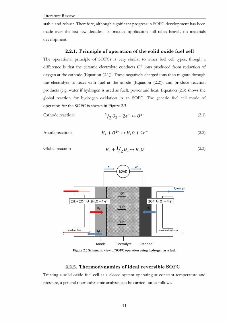
2.2.1. Principle of operation of the solid oxide fuel cell
The operational principle of SOFCs is very similar to other fuel cell types, though a
difference is that the ceramic electrolyte conducts O2- ions produced from reduction of
oxygen at the cathode (Equation (2.1)). These negatively charged ions then migrate through
the electrolyte to react with fuel at the anode (Equation (2.2)), and produce reaction
products (e.g. water if hydrogen is used as fuel), power and heat. Equation (2.3) shows the
global reaction for hydrogen oxidation in an SOFC. The generic fuel cell mode of
operation for the SOFC is shown in Figure 2.3.
Cathode reaction: 12⁄ 𝑂2 + 2𝑒
− ↔ 𝑂2− (2.1)
Anode reaction: 𝐻2 + 𝑂2− ↔ 𝐻2𝑂 + 2𝑒
− (2.2)
Global reaction 𝐻2 +12⁄ 𝑂2 ↔ 𝐻2𝑂 (2.3)
Figure 2.3 Schematic view of SOFC operation using hydrogen as a fuel.
2.2.2. Thermodynamics of ideal reversible SOFC
Treating a solid oxide fuel cell as a closed system operating at constant temperature and
pressure, a general thermodynamic analysis can be carried out as follows.

Literature Review
12
From the first law of thermodynamics, the total change in internal energy, ΔU, of a closed
system is:
∆𝑈 = 𝑄 −𝑊 (2.4)
where Q – is the heat added to the system; W – work done by the system.
The total work produced by the system is divided into work associated with mechanical
changes and work associated with other sources (e.g. magnetic, electrical, etc.)29. Here, only
electrical work is considered. Hence the Equation (2.4) is refined as follows:
∆𝑈 = 𝑄 − 𝑃∆𝑉 −𝑊𝑒𝑙𝑒𝑐 (2.5)
where PΔV is the expansion/compression work; Welec – electrical contribution to the work.
For a reversible change at constant temperature, the heat transferred is given by:
𝑄 = 𝑇∆𝑆 (2.6)
where S- is the entropy change.
The change in Gibbs free energy, ΔG, for a system operating at constant temperature and
pressure is given by:
∆𝐺 = ∆𝐻 − 𝑇∆𝑆 (2.7)
and the enthalpy change is defined as:
∆𝐻 = ∆𝑈 + 𝑃∆𝑉 (2.8)
Substitution of Equations (2.5) and (2.8) into (2.7) results:
∆𝐺 = −𝑊𝑒𝑙𝑒𝑐 (2.9)
This is the maximum electrical energy available in an external circuit, which is equal to the
number of charges multiplied by the maximum potential difference, which is the reversible
cell potential, E°rev, and is given by:
𝐸°𝑟𝑒𝑣 = −
∆𝐺°
𝑛𝐹
(2.10)
2.2.3. The Nernst Equation
The reversible cell potential given by Equation (2.10) is the potential for SOFC with
reactants and products in their standard state with activities, ai=1. Due to the temperature
dependency of Gibbs free energy change (Equation (2.7)), the intrinsic temperature
dependence of a reversible potential is evident.
In SOFC systems the activities of reactants and/or products are approximated to partial
pressures. Deviation of the latter from their standard state is reflected in the Nernst
potential, where the correction of the reversible cell potential is made as follows:

Literature Review
13
𝐸𝑟𝑒𝑣 = 𝐸
°𝑟𝑒𝑣 −
𝑅𝑇
𝑛𝐹ln𝑎𝑝𝑟𝑜𝑑𝑢𝑐𝑡𝑠
𝑎𝑟𝑒𝑎𝑐𝑡𝑎𝑛𝑡𝑠
(2.11)
The Nernst equation for oxidation of hydrogen shown in Equation (2.3) is calculated using
partial pressures in place of species activities with reaction stoichiometry 1, 0.5 and 1 for
hydrogen, oxygen and water, respectively:
𝐸𝑟𝑒𝑣 = 𝐸°𝑟𝑒𝑣 +
𝑅𝑇
2𝐹ln (
𝑝𝐻2𝑝𝑂21/2
𝑝𝐻2𝑂)
(2.12)
2.2.4. Fuel cell polarisation
Once a potential is applied to a fuel cell a current flows from anode to the cathode and the
voltage of the cell changes, this process is known as polarisation. A schematics of a typical
fuel cell polarisation curve as a function of current density is shown in Figure 2.4.
At open circuit (when no current is drawn from the cell) the cell voltage is lower than the
thermodynamically predicted voltage due to energy loss under reversible condition, so-
called open circuit losses (losses due to internal current and parasitic reactions), fuel
crossover and mixed potentials.
Figure 2.4 Schematic of a typical current – voltage or polarisation curve that shows the operating cell voltage with activation, ohmic and concentration potential losses.
The actual cell potential is lower than the reversible potential, Erev, due to three different
mechanisms of irreversible losses:
activation polarisation
ohmic polarisation
concentration polarisation
Conentration losses cause decrease of cell potential to zero
Cell
Voltage / V
Current density / A m-2
Linear drop in cell potential
due to ohmic losses
Cell potential losses due to
activation overpotential
Reversible potential - Nernst Potential (OCV)

Literature Review
14
Considering this the cell potential is then given by:
𝐸𝑐𝑒𝑙𝑙 = 𝐸𝑟𝑒𝑣 − 𝜂𝑎𝑐𝑡 − 𝜂𝑐𝑜𝑛𝑐 − 𝜂𝑜ℎ𝑚𝑖𝑐 (2.13)
where ηact, ηconc, ηohmic – are the activation, concentration and ohmic potential losses.
From Figure 2.4 it follows that activation polarization primarily occurs at low current
density, while concentration polarization occurs predominantly at high current density. The
next subsections describe each of the polarisation losses separately.
2.2.4.1. Activation overpotential
Activation overpotential is an additional potential required to overcome the energy barriers
for oxygen reduction (Equation (2.1)) and hydrogen oxidation (Equation (2.2)) reactions at
the electrode/electrolyte interfaces. Activation overpotential becomes significant at low
current density region as the rates of those electrochemical reactions are low.
The Butler-Volmer equation relates the electrode activation overpotential, ηact and the
current density, j as follows:
𝑗 = 𝑗𝑜 [exp (
𝛼𝑎𝑛𝐹(𝐸 − 𝐸𝑟𝑒𝑣)
𝑅𝑇) − exp (−
𝛼𝑐𝑛𝐹(𝐸 − 𝐸𝑟𝑒𝑣)
𝑅𝑇)]
(2.14)
Or in simplified form:
𝑗 = 𝑗𝑜 [exp (
𝛼𝑎𝑛𝐹𝜂𝑎𝑐𝑡𝑅𝑇
) − exp (−𝛼𝑐𝑛𝐹𝜂𝑎𝑐𝑡𝑅𝑇
)] (2.15)
where j0 is the exchange current density, 𝛼𝑎 and 𝛼𝑐 are the anodic and cathodic charge
transfer coefficients respectively, n – number of electrons transferred in reaction, F –
Faraday constant, R - Universal gas constant, T – operating temperature, E – cell voltage.
The limiting case of the Butler-Volmer equation is the Tafel equation, which expresses
activation for cathodic reaction (E<<Erev) as follows:
𝜂𝑎𝑐𝑡 = 𝑎 − 𝑏log(𝑗) (2.16)
And similarly for anodic reaction (E>>Erev)
𝜂𝑎𝑐𝑡 = 𝑎 + 𝑏log(𝑗) (2.17)
where a and b are Tafel equation constants for a given reaction and temperature.
High electrocatalitic activity of electrodes with large values of j0 is favourable, as
electrochemical reaction rate is fast and large current densities can be obtained with lower
activation overvoltage.
2.2.4.2. Concentration overpotential
Concentration overpotential arises as a result of the slow mass transport of reactants
reaching the reaction sites and the products leaving them. This leads to depletion of

Literature Review
15
reactants and accumulation of products at reaction sites. This overpotential is more
dominant at high current densities when the slow rate of mass transport is unable to meet
the required high demand of current output.
Concentration overpotential is induced by the concentration gradient which is caused by
the differences in partial pressures/ concentrations of reactants and products between the
bulk stream and reaction sites (electrode/electrolyte interface)30.
The concentration overpotential at each electrode can be calculated from the local partial
pressures of each reacting species (H2, O2 and H2O for typical SOFC operation) that are
transported between the bulk and reaction sites (electrode/electrolyte interface)31:
Cathode 𝜂𝑐𝑜𝑛𝑐 =𝑅𝑇
2𝐹ln ([
𝑝𝑂2𝑏𝑢𝑙𝑘
𝑝𝑂2𝑟𝑒𝑎𝑐𝑡
]
1/2
)
(2.18)
Anode 𝜂𝑐𝑜𝑛𝑐 =𝑅𝑇
2𝐹ln (
𝑝𝐻2𝑏𝑢𝑙𝑘 𝑝𝐻2𝑂
𝑟𝑒𝑎𝑐𝑡
𝑝𝐻2𝑟𝑒𝑎𝑐𝑡 𝑝𝐻2𝑂
𝑏𝑢𝑙𝑘)
(2.19)
where react. – stands for reaction zone.
Application of Equations (2.18) and (2.19) for determination of concentration
overpotential is not straightforward due to complexity associated with measurement of
local reaction concentrations/ partial pressures.
An alternative equation for calculation of concentration overpotential as a function of
limiting current density at which the partial pressures of reactants at the reaction sites tend
to zero30,32 is as follows:
𝜂𝑐𝑜𝑛𝑐 = 2.303
𝑅𝑇
𝑛𝐹log (
𝑗𝑙𝑖𝑚𝑗𝑙𝑖𝑚 − 1
) (2.20)
where jlim is the limiting current density.
2.2.4.3. Ohmic overpotential
Ohmic losses are due to electrical resistance that arises from fuel cell components: cathode,
anode, electrolyte, interconnects. From Ohm’s law, the ohmic polarization is linearly
dependent on the cell current, I, and can be found as follows:
𝜂𝑜ℎ𝑚𝑖𝑐 = 𝐼𝑅𝑐𝑒𝑙𝑙 (2.21)
where 𝜂𝑜ℎ𝑚𝑖𝑐 is ohmic polarisation; Rcell is the overall resistance of the cell.
Literature Review
16
The ohmic losses can be improved by increase of conductivity of the cell components and
reduction in the path length for current flow. Hence ohmic polarisation, 𝜂𝑜ℎ𝑚𝑖𝑐 , can be
expressed as follows:
𝜂𝑜ℎ𝑚𝑖𝑐 = 𝐼∑
𝑙𝑖𝐴𝑖𝜎𝑖
𝑖
(2.22)
where li – the corresponding path length in cell component i, Ai – the cross-sectional area
of the component i, σi is the conductivity of the component i.
2.2.5. Geometry of solid oxide fuel cells
Depending on geometry there are three main configurations of SOFC: tubular, planar and
monolithic23,28. The schematic view of all three SOFC modifications are shown in Figure
2.5-Figure 2.10. Generally, both tubular and planar SOFC are designed as electrolyte-
supported, anode-supported and cathode-supported cells, where the support is the thickest
part of the cell23. However, more attention has been devoted by planar SOFC, as it was
reported to have more compact design and higher volume of specific power23.
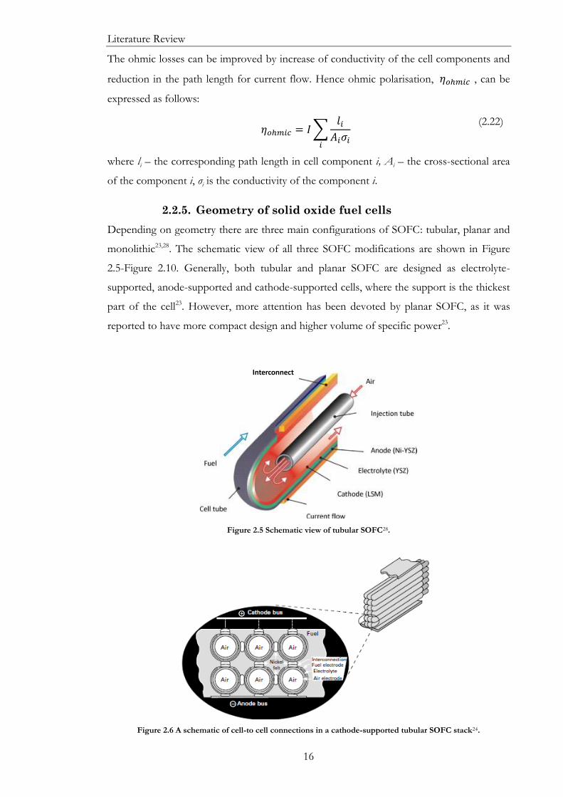
Figure 2.5 Schematic view of tubular SOFC28.
Figure 2.6 A schematic of cell-to cell connections in a cathode-supported tubular SOFC stack24.
Interconnect

Literature Review
17
Figure 2.7 Schematic of cell configuration in an anode-supported planar SOFC stack24.
Figure 2.8 Schematic view of planar SOFC28.
Figure 2.9 A schematic of the ‘segmented-in-series’ design adopted by Rolls-Royce24.
In a monolithic SOFC, layers of electrodes are placed in a certain way so that anode and
cathode form two channels for fuel and air. Three layers of the system are then sintered
into one piece. Monolithic models combine some positive properties from both tubular
and planar systems.

Literature Review
18
Figure 2.10 Schematic view of monolith-type SOFC33.
2.2.6. Fuel flexibility of solid oxide fuel cells
Solid oxide fuel cells are flexible to a range of fuels, primarily due to the high operating
temperature. They differ from PEM fuel cells which primarily operate on hydrogen gas
(although other liquid fuels such as methanol are possible), whereas other hydrocarbons
can be used instead in SOFCs. The following reaction equations illustrate electrochemical
conversion of carbon monoxide and methane (used as fuels) in SOFCs.
Carbon monoxide (CO):
Anode reaction: 2(CO + O2- → CO2 + 2e-) (2.23)
Cathode reaction: O2 + 4e- → 2O2- (2.24)
The overall cell reaction: 2CO + O2 → 2CO2 (2.25)
At high temperature, there is a side reaction of oxidation of carbon monoxide with water to
carbon dioxide and hydrogen gas, which is a called the water-gas shift reaction23:
CO + H2O → CO2 + H2 (2.26)
Methane (CH4):
Anode reaction: CH4 + 4O2- → CO2 + 2H2O + 8e- (2.27)
Cathode reaction: 2(O2 + 4e- → 2O2−) (2.28)
The overall cell reaction: CH4 + 2O2 → CO2 + 2H2O (2.29)
2.2.7. Oxide-ion electrolyte in SOFCs
The performance of fuel cells largely depends on the electrolyte. It is generally preferable
for electrolytes to have high ionic conductivity and stability. The nature of the electrolyte
dictates the operating temperature of the fuel cell.
Literature Review
19
Apart from the relatively high oxygen-ion conductivity, there are other criteria for solid
electrolytes such as: stability compared to other cell components, adequate thermal and
mechanical properties (strength, toughness, mechanical and thermal shock resistance),
structural and thermodynamic stability (in fuel and oxidising conditions). The thermal
expansion coefficient of the electrolyte should match with other cell components. The
ionic transport number of the electrolyte should be close to unity, otherwise there will be
thermodynamic efficiency losses proportional to the electronic transport component34.
There are four main electrolyte systems applied in SOFCs and they are based on zirconia
(ZrO2), ceria (CeO2), lanthanum gallate (LaGaO3) and bismuth (Bi2O3) oxides. With respect
to fuel cell operating conditions, the most stable is the zirconia-based system, followed by
lanthanum gallate, ceria and bismuth oxide systems34. The oxides can be used separately or
together (mostly two of them) to increase the stability in a reducing environment34. For
instance, bi-layer structures usually contain a layer of doped zirconia on ceria or bismuth
oxide. Zirconia- and ceria-based electrolytes are relatively inert compared to doped bismuth
oxides, which become reactive and thus their stability during the operational time of the
stack significantly decreases.
Yttria-stabilised zirconia (YSZ)
Zirconia-based electrolyte is commonly used in solid oxide fuel cells operated at high (800-
1000 C) and intermediate (600-800 C) temperatures35, as it fulfils the above mentioned
electrolyte requirements. Zirconium is abundant in the Earth’s crust (165 parts per million
by weight36) and consequently has relatively low cost. The electronic transport number of
zirconia is small compared to other solid electrolytes in the oxygen partial pressure range
(>10-30 atm)35. This is a typical pressure range in fuel cell applications.
Zirconium oxide exists in three different phases: monoclinic, tetragonal and cubic37. Pure
zirconium oxide (ZrO2) is a monoclinic structured oxide at room temperature, with low
ionic conductivity. Monoclinic zirconia (m-ZrO2) is stable at ambient temperature, while
cubic (c-ZrO2) is stable from 2350 °C up to a melting temperature of 2680 °C and
tetragonal (t-ZrO2) is a metastable transition stage between m-ZrO2 and c-ZrO234. During
the heating process, at around 1170 C monoclinic ZrO2 transforms to tetragonal and at
2350 C from tetragonal to cubic34. These transformations are reversible on reducing the
temperature back to ambient, so that c-ZrO2 reverts to t-ZrO2 and then back to m-ZrO2.
Reverse transformations are followed by rapid volume change and disintegration of
material. Doping with a lower-valent oxide (e.g. yttria - Y2O3) can be applied to stabilise the
cubic and tetragonal structures at low temperature where they are mostly used. As
tetragonal phase is meta-stable and cubic phase is fully-stable the respective

Literature Review
20
dopant/stabiliser amount is needed for each of the phase. The tetragonal phase is stabilised
by adding stabilisers up to 4 mole % of cation, while the cubic phase requires addition in
excess of about 8 mole % of Y2O3. Cubic zirconia is known to be the most ionically
conductive among all three phases.
The following divalent and trivalent oxides can be used as potential zirconia dopants: CaO,
MgO, Y2O3, Sc2O3, Yb2O3, GdO3 and some other rare earth metal oxides. However, it has
been found38 that the stabilisers which produce cubic zirconia with best ionic conductivity
are those with a cation of similar size to that of Zr4+. The lattice conductivity obtained after
stabilisation is higher for trivalent metal compared to divalent metal oxide dopants38.
Among trivalent stabilisers the most common and well-developed is yttrium oxide (Y2O3).
A stabiliser has two main functions: the first one is to stabilise the structure of tetragonal or
cubic phase, while the second is to generate oxygen-ion vacancies to allow oxygen ion
diffusion. Substitution of Zr4+ ion with lower valent cation (e.g.Y3+) in the crystalline lattice
creates vacancies in the oxygen sub-lattice. This process can be expressed with Kroger-
Vink notation as follows:
𝑌2𝑂3𝑍𝑟𝑂2→ 2𝑌𝑍𝑟
′ +𝑉𝑂∙∙ +3𝑂𝑂
𝑥 (2.30)
The created vacancy (𝑉𝑂∙∙
) is mobile and allows oxygen ions to migrate through the lattice
when a certain activation energy level is overcome. Equation (2.30) explains the
phenomenon of oxygen ion conductivity by stabilised zirconia electrolyte, in this case
yttria-stabilised zirconia (YSZ).
As dopant level is increased the conductivity of stabilised zirconia similarly increases.
Higher amount of dopant leads to an increase in oxygen vacancy formation and hence
ionic conductivity of solid electrolyte39. At a certain level of dopant, created vacancies start
to interact, thereby limiting their mobility in the lattice and hence inhibiting the overall
conductivity35,39,40. As demonstrated by Fergus40 (see Figure 2.11) and other studies41,42 the 8
mol. % YSZ ((ZrO2)0.92(Y2O3)0.8) is the minimum amount of yttria needed to stabilise cubic
zirconia which exhibits the highest ionic conductivity.

Literature Review
21
Figure 2.11 Conductivity of yttria- and scandia-stabilised zirconia in air at 1000 °C40.
It has also been reported that the 9-10 mol.% ZrO2 -Y2O3 system shows no or very low
degradation of electrical properties34. Hence the YSZ electrolyte is used in this research
project. It has an adequate mechanical strength (about 250-300 MPa) with reduction at
1000 C to about 150-200 MPa along with good ionic conductivity. The yttria content was
changed at early stages of the project to find an optimum trade-off between the ionic
conductivity, mechanical strength and cost of electrolyte material.
2.2.8. Diagnosis of solid oxide fuel cells using EIS
Electrochemical impedance spectroscopy (EIS) is an electrochemical technique that has
been widely applied to distinguish individual losses in SOFCs, including oxygen reduction
reaction kinetics, mass-transport and electrolyte membrane resistance43–45. Detailed
overview of this technique is given in the next Chapter in Section 3.4.3. In this subsection
the main focus is given to application of EIS in SOFC studies to the resistivity of the solid
electrolyte.
One of the common applications of the EIS is the analysis of a YSZ conduction
properties46. In a solid electrolyte cell the overall electrolyte resistivity is governed by the
migration of oxygen ions within the lattice and between the grains (so called intra-grain
resistivity), and grain boundary (or inter-grain) resistivity, the latter explained by blocking of
migrating oxygen ions at the grain boundaries. Intra-grain electrical conductivity of zirconia
electrolyte is found to be mainly due to the dopant type and its concentration, and some
other aspects such as phase assemblage, and grain porosity34. An idealised impedance
spectrum of a zirconia electrochemical cell with electrodes consists of three semi-circles in

Literature Review
22
the Nyquist plot47 (Figure 2.12). A corresponding equivalent circuit for that system includes
three parallel R-C elements connected in series.
Figure 2.12 An idealised Nyquist plot of a zirconia electrochemical cell with electrodes and its equivalent circuit. The three semi-circular arcs correspond to conductivity within the grain, grain boundaries and
electrodes, respectively47.
The arcs attributing to the conductivity across the grain and grain boundaries in the solid
electrolyte appear at higher frequencies, while the conductivity at the electrolyte/electrode
interface is more prominent at lower frequencies46,47. The first two semi-circles tend to
diminish with increase of temperature due to significantly reduced intra-grain and inter-
grain resistance of the electrolyte47. As a result, the first two R-C elements are typically
replaced by a single resistor that represents the overall electrolyte resistivity.
EIS is also widely used to diagnose performance of SOFCs with respect to operating
conditions and cell components. For instance, humidification of supplied fuel significantly
affects the operation of a fuel cell. This may be confirmed with measured in-situ EIS data
where humidified fuel (e.g. hydrogen) results in lower resistance compared to dry fuel43.
Working temperature is another common parameter used to analyse performance of the
SOFC.
Overall, EIS is being commonly used in SOFC studies because it provides individual
fundamental information on each of the phenomena occurring at each interface as well as
the bulk electrolyte conductivity. However, analysis and interpretation of impedance data is
not straightforward, as data analysis has to correlate with other experimental information to
verify the chosen equivalent electrical circuit for data fitting.

Literature Review
23
2.2.9. Direct Carbon Fuel Cell
In liquid metal anode SOFCs carbon (coal) can undergo direct electrochemical oxidation to
carbon dioxide. A brief review of the common direct carbon fuel cells (DCFC) is given in
this section to set the scene.
The direct carbon fuel cell (DCFC) was first reported by Sir William Grove in 183948,49.
After several attempts, Dr. William Jacques was the first to build a direct carbon fuel cell in
1896, using a molten hydroxide electrolyte49. Since that time, many researchers have
worked to optimize this technology by applying new materials and improving the cell
design. The most recent designs of DCFC are being developed and proposed by the
Lawrence National laboratory, Cell Tech Power LLC and SRI International simultaneously
with Scientific Applications & Research Associates (SARA), Inc.
The direct carbon fuel cell incorporates the characteristics of MCFCs and SOFCs, using
solid carbon as a fuel instead of a typical gaseous fuel (e.g., hydrogen or methane).
According to the type of electrolyte used in the system, DCFCs are classified into three
main types: those with molten hydroxide electrolyte, molten carbonate electrolyte and solid
oxide electrolyte (typically YSZ). Electrical power is generated directly by introducing solid
carbon, followed by its electrochemical oxidation to CO2. The net cell reaction is:
C(s) + O2 (g) CO2 (g), E0 = 1.02 V (2.31)
DCFCs have numerous benefits, including high thermodynamic efficiency, which makes
them advantageous over conventional molten carbonate or solid oxide fuel cells. The
entropy change for the overall cell reaction is positive (ΔS = 1.6 J K-1 mol-1 at 600C)
resulting in higher Gibbs free energy change (ΔG = -395.4 kJ mol-1 at 600C) than the
standard enthalpy change (ΔH = -394.0 kJ mol-1 at 600C)4. Therefore, theoretical
electrochemical conversion efficiency of DCFC for the net cell reaction is greater than
100%.
Due to their low carbon emissions, DCFCs are considered to be a more environmentally
friendly option than existing coal-firing plants. Cao et al.4 stated a 50% reduction in CO2
emissions compared with conventional power plants. This is explained by direct
electrochemical oxidation of carbon at the anode with no reaction with air. Therefore, the
produced CO2 is free from nitrogen as well as combustion products, such as SO2, NOx,
etc., that are formed in combustion boilers. Almost pure CO2 produced in a DCFC is then
suitable for further applications or CCS (carbon capture and storage). This advantage
makes this technology exceptionally promising in certain regions of the world, where coal

Literature Review
24
remains the primary energy resource (e.g. US, China, Former Soviet republics, etc.). To
date, the US and China remain the highest CO2 emitters around the world4.
The carbon required for DCFC systems is available from a variety of fuels, such as coal,
biomass, and petroleum coke, which makes this technology even more attractive and
promising. The system simplicity, absence of heat engines and reformers makes this
technology adaptive directly near coal mines.
A schematic configuration of a direct carbon fuel cell constructed by Lawrence National
Laboratory (LLNL, Livermore, CA) is shown in Figure 2.13. A 32% Li2CO3-68% K2CO3
molten salt mixture was used as the electrolyte. The operating current density varied from
58 to 124 mA cm-2 at cell voltage of 0.8 V, which is 80% of its thermodynamic voltage4.
Figure 2.13 a)LLNL DCFC configuration with carbon particle anode, b) performance of LLNL DCFC4.
A novel arrangement for DCFC was patented by Balachov and co-workers4 at SRI
International, where the main fuel cell component was a U-tube, consisting of a cathode
current collector, cathode (lanthanum strontium manganite (LSM)), electrolyte – yttrium-
stabilized zirconia (YSZ), anode current collector. The tube was immersed into a liquid
anode (Li2CO3+K2CO3+Na2CO3). The design is illustrated in Figure 2.14a. The authors
tested a variety of fuels (coal, tar, coke, acetylene, plastic, etc.). Reported power density was
greater than 100 mW cm-2 at 950C (Figure 2.14b).
(a) (b)

Literature Review
25
Figure 2.14 Configuration of the SRI direct carbon fuel cell (a), performance of SRI direct carbon fuel cell (b)4.
However, there are some ongoing technical challenges for DCFCs. They are primarily
associated with high operating temperatures that require thermostable materials (e.g.
ceramic, metal alloys) for stack components, which are typically expensive22,49.
2.3. Liquid Metal Electrode Electrochemical
Systems
The generic construction of a liquid metal electrode solid oxide fuel cell (LME SOFC) is
illustrated in Figure 2.15. The arrangement is ostensibly identical to a conventional solid
oxide fuel cell except that the anode is a molten metal. Fuel is fed to the electrode and
oxidized products are generated in the same way. The difference is that both gaseous and
solid fuel can be fed directly and effectively converted with no pretreatment stage.
Figure 2.15 Operation of liquid metal electrode reactor in fuel cell and electrolyser mode.
Figure 2.15 also shows the potential for operation in electrolyser mode. This concept has
the cell fed with CO2 and steam (H2O) that are electrochemically converted to synthesis gas
(a) (b)
Anode current collector
Fuel + liquid anode
Electrolyte
Cathode
Cathode current collector
Oxidizer inlet
Oxidizer outlet

Literature Review
26
(a mixture of hydrogen and carbon monoxide), that can be used to produce liquid fuel (i.e.
via the Fischer-Tropsch process) or used in a fuel cell directly50.
2.3.1. Liquid Metal Electrode Solid Oxide Electrolyser
As shown in Figure 2.15 a molten metal anode can be applicable for electrolytic reduction
of carbon dioxide and/ or steam in solid oxide electrolysers (SOE). To understand how
molten metal operates in electrolyser mode, conventional technological characteristics of
SOE should be examined. Hence, this section briefly summarizes recent advances in SOE
technologies using carbon dioxide and steam to produce a gaseous mixture of carbon
monoxide and hydrogen, which is usually referred to as “synthesis gas” or “syngas”. The
present study focuses mainly on application of a liquid metal electrode in fuel cell mode,
though a possible application of molten electrode for water electrolysis has been also
explored briefly (refer to Chapter 9).
High temperature electrolysis of CO2 and steam for production of synthesis
gas
A significant amount of work has been done in this research area, as it seems to be a
promising technological solution for production of hydrogen (alternative energy fuel) and
carbon monoxide comprising the synthetic gas suitable for further applications51–54. It is a
favourable option that offers simultaneous reduction of carbon dioxide and steam that are
usually released into the atmosphere in conventional power plants.
Pati et al.53 have stated several advantages of SOE:
- Utilization of waste heat from nuclear waste and industrial processes to meet heat
requirements of SOE;
- Production of pure hydrogen, free from typical impurities (sulphur and CO).
However, the main drawback remains high power requirement for electrolysis of steam53.
Typical SOSE contains cathode and anode separated by oxygen-ion conducting YSZ
electrolyte. Steam is fed to the cathode, where it dissociates into H2 and O2-; the produced
oxygen ions migrate through electrolyte layer to the anode and are oxidized to produce
molecular oxygen:
Cathode reaction: H2O + 2e-O2- + H2 (2.32)
Anode reaction: O2- 2e- + 1/2 O2 (2.33)
By analogy to steam electrolysis the reduction of CO2 to CO using conventional SOEs
(with Ni-YSZ electrodes) has been reported recently55 demonstrating relatively good

Literature Review
27
performance. The reduction reaction is carried out at the cathode side of the SOE as
follows:
Cathode reaction: CO2 + 2e- O2- +CO (2.34)
However, there are still concerns regarding the stability of Ni-YSZ components, as they
can be damaged by a CO-CO2 environment. Therefore, further investigation on more
stable electrodes or lower energy requirements is needed.
The process of steam dissociation is regulated by applied potential difference between
electrodes and requires significant power (ca. 70% of the total energy used). It was
suggested that energy requirements might be reduced by introducing new anode materials,
as liquid metals53.
Several studies53,56 reported an adequate performance of solid oxide steam electrolyser
(SOSE) where molten tin was employed as anode. This technological solution can be also
applied for CO2 electrolysis.
The design of such a steam electrolyser with liquid tin anode and Ni-YSZ cermet cathode
is presented in Figure 2.16. Successful production of hydrogen at temperature range from
900 to 1000 C was achieved whereby high temperature steam was fed to the cathode,
while solid carbon - to the liquid tin anode.
Figure 2.16 Schematic of solid oxide membrane electrolyser for waste to hydrogen and syngas conversion53.
The main concept of such electrolytic cell was the introduction of a reductant that would
lower the energy requirements for steam electrolysis by reducing the chemical potential of
oxygen53. SOE or SOFC with conventional solid electrodes cannot handle a solid
reductant, except those that use molten metal electrodes, where reaction between solid and
liquid is more favourable.

Literature Review
28
In such a SOEC system the liquid metal has been used as the anode. There are no literature
studies that present solid oxide electrolysis using liquid metal as the cathode for reduction
of species within the melt. Hence this field of the LME systems is open for further
research. Early work on water/steam electrolysis using a molten tin electrode in solid
oxide systems is demonstrated in Chapter 9 of this thesis.
2.3.2. Liquid Metal Anode SOFCs
The liquid metal electrode resides in a layer between the fuel chamber (gaseous or solid
fuel) and the solid electrolyte (Figure 2.17). The oxygen reduction reaction occurs at the
cathode/electrolyte interface generating oxygen ions, which then migrate through the solid
electrolyte, typically represented by yttria-stabilised zirconia (YSZ), to the liquid metal
anode. The O2- ions react electrochemically with the liquid metal, generating metal oxide
which is the active species for the oxidation of the fuel (gaseous or solid - carbon and
hydrogen in the diagram), producing carbon dioxide or water respectively. However, the
exact mechanism occurring and the species involved in the liquid metal anode media are
not well defined and depend upon the metal used and operating conditions.
The molten metal blocks direct contact of electrolyte with gaseous impurities and hence
reduces electrolyte degradation by inhibiting the reaction between contaminants and
electrolyte6. Moreover, the fuel contaminants can become a fuel source themselves as they
undergo electrochemical oxidation. All of the electrolyte surface in contact with the anode
is available to supply a flux of oxide ions for reaction - there is no need to engineer a
complex ceramic metal (cermet) electrode with optimized triple phase boundary (TPB) as is
necessary in conventional SOFCs57,58.
Figure 2.17 Schematic showing operation of LMA SOFC with (a) hydrogen and (b) solid carbon, as the fuel.

Literature Review
29
2.3.2.1. Operation of Liquid Metal Anode SOFCs
The liquid metal anode acts as an intermediary for the oxidation of fuel6. Taking a molten
metal (M) and hydrogen as a fuel, the reactions at the LMA-SOFC anode follows the
generic mechanism:
𝑀(𝑙) + 𝑛𝑂2− ↔ 𝑀𝑂𝑛 + 2𝑛𝑒
− (2.35)
𝑀𝑂𝑛 + 𝑛𝐻2 ↔ 𝑀 + 𝑛𝐻2𝑂 (2.36)
The first reaction (2.35) proceeds at the liquid anode-electrolyte interface, whereas the
second reaction (2.36) occurs at the fuel-anode interface. The oxide ions (O2-) are delivered
from the cathode via the electrolyte. The state of oxygen in the metal varies with operating
conditions. When using tin, oxygen may form oxide or suboxide, or remain dissolved in the
melt59. The state of oxygen may vary, though it has no particular effect on the overall
reaction, which is the sum of the first and second reactions:
H2+ O2- H2O+ 2e- (2.37)
This reaction (2.37) is applicable to any liquid metal anode SOFC system including Sn or
Cu60.
2.3.2.2. Thermodynamics of LMA SOFC operation
The maximum electrical voltage generated by an electrochemical system can be determined
via the equilibrium electrode potential (EN), expressed by the Nernst equation (2.38) as
follows:
𝐸𝑁 = 𝐸
°𝑟𝑒𝑣 −
𝑅𝑇
𝑛𝐹 ∑𝑣𝑖 ln 𝑎𝑖𝑖
(2.38)
where ai and vi are the activities (fugacities for gases) and stoichiometric coefficients of all
reactants and product species i, R is the molar gas constant, 8.314 J mol-1 K-1, T is absolute
temperature and E°rev is the standard electrode (equilibrium) potential of the reaction that
can be defined from the Equation (2.39):
𝐸°𝑟𝑒𝑣 =
−∆𝐺𝑟0
(𝑛𝐹)
(2.39
where ΔGr0 is the Gibbs free energy change for the global reaction of H2 oxidation (H2 +
1/2O2 H2O), n – number of electrons transferred during electrochemical reaction and F
is the Faraday’s constant.

Literature Review
30
The standard equilibrium potentials of several metal-metal oxide couples as a function of
temperature are shown in Figure 2.18. The data for the figure was generated using the
chemical reaction and equilibrium software HSC Chemistry 6.1 (Outotec, Finland).
It can be seen that the cell voltage is expected to decrease with increasing temperature, as a
result of the negative entropy change associated with the reactions. However, the voltage
obtained under operating conditions (with a net current flowing) is difficult to predict. In
addition to the usual loss mechanisms associated with reaction kinetics, ohmic and mass
transport limitations, cell voltage will depend on the actual reaction at the anode: whether it
is directly with dissolved fuel or the oxidation of the metal to oxide (electrochemical
reaction) followed by oxidation of the hydrogen by the oxide (chemical reaction).
If the reaction is directly with the fuel then conventional fuel cell reaction OCVs will hold,
which are generally higher than those for the reaction with the metal. Therefore, from a
thermodynamic perspective, it may be preferable for the metal to have a low affinity for
oxygen and a high solubility of fuel and oxygen.
Figure 2.18 Effect of temperature on standard equilibrium cell potentials for various metal oxidation reactions.
Battery Effect
The use of LMAs can have an additional positive impact on fuel cell performance by
creating the so-called ‘battery’ buffering effect. It is well known that SOFCs (similar to
other fuel cells) can be detrimentally affected by power demand surges during operation,
since such surges can cause fuel starvation, which in turn may cause irreversible structural
changes at the electrodes. The presence of a certain amount of LMA acts as a metal-oxygen
0
0.2
0.4
0.6
0.8
1
1.2
1.4
500 700 900 1100 1300 1500
Stan
dar
d e
qu
ilib
riu
m p
ote
nti
al /
V
Temperature / K

Literature Review
31
battery, where the metal itself is oxidised to provide sufficient load6,12,61. The oxidised metal
can be reduced again by the fuel fed into the anode when normal load is resumed.
2.3.2.3. Ideal Potential
According to the Nernst Equation, the ideal potential for LTA SOFC can be derived
similar to any kind of hydrogen fuel cell and expressed by the following equation62:
𝐸𝑁 =−∆𝐺0
2𝐹+𝑅𝑇
2𝐹ln(
𝑎𝐻2(𝑎) × 𝑎𝑂2(𝑐) 12
𝑎𝐻2𝑂(𝑎))
(2.40)
The simplified form of the above Equation (2.40) is presented below62:
𝐸𝑁 =
𝑅𝑇
4𝐹ln (
𝑎𝑂2(𝑐)
𝑎𝑂2(𝑎) )
(2.41)
where EN is the ideal Nernst potential, ΔG0 is the Gibbs free energy change for the
reaction of production of water from H2 and O2 (H2 + 1/2O2 H2O).
In their fundamental analysis of the LTA SOFC, Gemmen et al.62 explained different types
of electrochemical equilibrium that occur in the system, such as Anode Gas – Liquid Metal
Equilibrium, Liquid Metal – Metal Oxide Equilibrium, and also suggested the pattern of
non-equilibrium operation of the system.
For the first case of equilibrium it was assumed that the species in the anode gas phase are
in equilibrium with species in the liquid metal. This is possible due to the equal chemical
potentials of species in gas phase and in molten metal phase. And hence, at given
concentrations of hydrogen and water in the anode gas, the given oxygen activity remains
independent of the form in which the oxygen is incorporated (oxide, dioxide, sub-oxide or
dissolved oxygen). Subsequently, Equation (2.41) can be written as62:
𝐸𝑁 =
𝑅𝑇
4𝐹ln (
𝑎𝑂2(𝑐)
𝑎𝑂2(𝑚) )
(2.42)
where 𝑎𝑂2(𝑚) is activity of oxygen within molten metal.
The activity of oxygen within the molten metal (Sn) is the same, and is equal to the activity
of oxygen in the anode gas phase; hence the ideal potential of the system expressed by
Equations (2.41) and (2.42) are equivalent.
The second case presented by Liquid Metal – Metal Oxide Equilibrium, where there is a
case of formation of metal-oxide phase due to sufficiently large oxygen concentration in
the anode. As a result, metal-oxide equilibrates with liquid metal and oxygen at the anode.
Assuming that until there is enough oxygen at the anode side to consume all the metal (so

Literature Review
32
that there is no metal oxide), the ideal potential is only dependent on the activity of oxygen
at the cathode side and working temperature62:
𝐸𝑁 =
−∆ 𝐺0𝑀−𝑀𝑂𝑛2𝐹
+𝑅𝑇
4𝐹ln(𝑎𝑂2(𝐶) )
(2.43)
where ΔG0 M-MOn is the change in Gibbs free energy for metal oxidation reaction (M+ (n/2)
O2 MOn).
In summary, it was shown that Equation (2.41) is applied for general cases; Equation (2.43)
is used if it is evident that both metal and metal-oxide exist (e.g. for battery mode, where
only conversion of M to MOn is possible). And finally, the Nernst equation expressed by
Equation (2.40) can be applied when H2 is available for the reaction of hydrogen
conversion to water.
In the following figure (Figure 2.19) Gemmen et al.62 presented the calculated Nernst
potentials over a range of temperature for all three cases (Sn+O2SnO2;
Sn+1/2O2SnO; H2+1/2O2H2O, where the system pressure is 1 atm; partial pressure
of O2 at cathode = 0.21 atm, hydrogen content is about 97%).
Figure 2.19 Ideal Nernst potentials for LTA SOFC for all three reactions62.
According to Figure 2.19, the actual OCV of the system is between two given potential
lines. The potentials shown provide a rough estimate of fuel cell performance but in
practice the system is not in equilibrium and as stated by Abernathy et al.6 a higher oxygen
activity is present within liquid anode than within the anode gas stream (where H2 is
present) due to some resistance of oxygen flow in liquid melt. At a particular current
density, oxygen activity grows considerably compared to oxygen activity in the anode gas
phase, leading to formation of metal oxide. The metal oxide produced then blocks the
electrolyte interface, reducing the overall cell performance and can pose significant
problems62.

Literature Review
33
2.3.3. Liquid Tin Anode SOFC
Liquid tin anode SOFCs (LTA SOFC) have been demonstrated with a variety of fuels,
including gaseous, solid and liquid carbonaceous fuels that do not require any processing,
reforming or pretreatment to remove sulphur. The power density reported was >160 mW
cm-2 with hydrogen and 120 mW cm-2 with JP-8 fuel62. Operated at 900 C, a layer of
molten tin (6 mm) was exposed to humidified H2 gas (3% H2O). From the analysis of
transient time characteristics, the oxygen (oxide) diffusion coefficient of 1×10⁻³ cm2 s-1 was
deduced from test results. The value differs significantly from previously measured
literature values62. Oxide diffusivity is one of the most critical fundamental parameter that
determines cell performance. Inconsistencies in literature reported values call for further
work to develop robust methods for the determination of this parameter.
Physical and chemical properties of tin and tin-oxygen systems
Abernathy et al. make the case for tin as a good candidate for LMA SOFCs6. A comparison
table (Table 2.2) summarises physical properties and abundances of various metals that can
be used as a liquid anode. The metal should have relatively low melting point (simplifying
operational conditions) and high boiling point. Tin has a low vapour pressure (9.87 × 10⁻⁴
Pa at 1000 0C) and hence, low volatility17, i.e. the anode is not vaporised into the fuel exit
stream during operation. Being technically easier to operate with, Sn remains the most
commonly used anode material for such LMA SOFC systems, though some researchers are
seeking alternative anode materials and suggest the use of metal alloys based upon tin.
Such factors as metal abundances in the Earth’s crust, annual production and associated
prices also have to be taken into consideration. Research studies so far have shown results
working with tin, copper and bismuth. Other metals may not be suitable due to health
hazards (Sb), high price (Ag) or low abundance (In).

Literature Review
34
Table 2.2 Common metals properties and abundances, prices (adapted from Abernathy et al.6).
Metal Tm,/ C Tb,/ C Price*/ $ kg-1
Abundance in Earth’s crust/
ppm
Reported studies using metal and/or
metal alloys
Aluminum 660 2520 1.7 83,000 - Antimony 631 1587 5.0 0.20 19,63 64–69
Bismuth 271 1564 16.3 0.063 21,60,63,70 Cadmium 321 767 2.7 0.10 - Copper 1085 2563 5.2 79 60 Indium 157 2073 390 0.05 19 Lead 328 1750 1.7 7.9 Pb - 19;Sn-Pb alloy-21;
Sn-Pb-Bi alloy-21, Tin 232 2603 13.9 2.5 6,12,13,15–17,20,59,62,64–73 Silver 962 2163 471 0.079 - Zinc 420 907 1.7 79 -
*The metal prices are taken from US Geological Survey Minerals Information Team, Mineral Commodity Summaries 2010.
Table 2.3 shows the chemical and physical properties of tin at a range of temperatures,
including the solubility of oxygen, hydrogen and sulphur. Electrical resistivity of tin at 1000
0C has a reasonable value of 67.1 µΩ cm compared to the resistivity of nickel (53.1 µΩ cm)
used in conventional ceramic metal (cermet) SOFC anodes17. The density of tin and nickel
at room temperature are 7.28 g cm-3 and 8.90 g cm-3, respectively. This makes tin an even
more preferable metal on the basis of weight17. High solubility of sulphur at high
temperatures74 in the melt is an attractive property of tin, allowing ‘dirty’ fuels to be used
without sulphur removal or fuel reforming.
Table 2.3 Thermophysical properties of tin6.
Property Temperature / C Value
Surface tension 232 5.44 mN cm-1 Viscosity 232 1.85 mN s m-2
Expansion on melting 232 2.3%
Density
800
6.58 g cm-3
1000 6.48 g cm-3
Resistivity
800
62.1 µΩ cm
1000 67.1 µΩ cm
Gas solubility-oxygen
536
0.000018 wt%
750 0.0049 wt%
Gas solubility- hydrogen
1000
0.04 cm3 H2/100 g Sn
1300 0.36 cm3 H2/100 g Sn
Gas solubility - sulphur
800
4.5 wt%
1000 8.0 wt%

Literature Review
35
The viscosity of liquid tin is not much greater than of liquid water75 at 20 °C, 1.002 mN s
m-2, hence the hydrodynamic properties of both fluids are similar. Low viscosity can be
exceptionally valuable if for instance a vigorous stirring or rotation inside the melt is
required. It may be also useful for circulation of liquid tin anode around the system.
One of the less attractive features of tin is its relatively high surface tension, and hence
poor wetting properties. Nogi et al.76 reported the surface tension of liquid tin measured by
the sessile droplet method as a function of temperature and oxygen partial pressure.
Surface tension values between 5.5 and 4.95 mN cm-1 were reported for the temperature
range of 227 and 827 °C at low oxygen partial pressure. This would primarily affect the
liquid tin/ solid electrolyte (typically YSZ) interface when a thin layer of tin is anticipated.
In order to resolve this issue an extra mechanical pressure has been applied by some
researchers16–18,63 on top of the liquid tin to reduce its contact angle and wet the surface of
electrolyte.
Reports on hydrogen solubility in liquid tin date back to the 1920’s. Abernathy et al.6 have
recently summarised the early papers on H2 solubility in liquid tin: a value of 9×10⁻⁵ at.% H
in tin at 1000 °C or 3.81×10⁻⁷ moles of H2/100 g Sn was measured by Bever et al.77 while
Iwase78 reported 1.4×10⁻² at.% H in tin at 1000 °C (5.9×10⁻⁵ moles of H2/100 g Sn). Clearly
a substantial difference of more than two orders of magnitude in the reported values is
evident, possibly due to variation in methods applied, as well as general difficulty of the
measurements.
The solubility of oxygen in liquid tin has been measured by Belford and Alcock79 using
electromotive force (EMF) measurements in the temperature range from 536 °C to 751°C
and extrapolated to cover the range from 232 °C to 1100 °C. Measured and predicted
values for oxygen solubility in liquid tin are shown in Table 2.4.
Table 2.4 Solubility of oxygen in liquid tin79 .
Temperature / °C Direct values /at.% [O] Method
536 0.0012 Measured
600 0.0042 Measured 700 0.0190 Measured
751 0.0360 Measured 780 0.0561 Predicted
Similarly Ramanarayanan and Rapp80 have reported solubility of oxygen in liquid tin using
(EMF) measurements in the temperature range of 750 to 950 °C. The following expression
was derived from experimental data obtained:
𝑁𝑂𝑠(𝑆𝑛) = 1.3 × 10⁵𝑒𝑥𝑝 (−
30000
𝑅𝑇) (2.44)

Literature Review
36
where 𝑁𝑂𝑠(𝑆𝑛) is the solubility of oxygen in at.%, R is the gas constant in cal K-1mol-1, and
T is the absolute temperature in K.
At a temperature of 780 °C (the operating temperature in present work) Equation (2.44)
predicts an oxygen solubility of 0.08 at.%.
The possible states of oxygen in liquid tin have been recently determined by Cahen et al.81
and presented in the form of Sn-O phase diagram (Figure 2.20). From the diagram the
solubility limit of oxygen is about 2 at.% at 1000 °C. Beyond this point tin dioxide (SnO2)
precipitates in the solution (melt). This number is almost twice that calculated by the
previous Equation (2.44) – 0.91 at.% at 1000 °C.
Figure 2.20 Sn-O phase diagram determined at 1 bar81.
Abernathy et al. have also attempted to determine the oxygen solubility in the liquid tin
anode in order to further refine the existing data in the literature6. An oxide ion flux was
assumed to be a measure for the dissolved oxygen concentration when currents of various
magnitude were supplied to the LTA SOFC at an operating voltage of 0.78 V (the potential
at which tin is suggested to convert to tin dioxide). As a result, a value of 0.8 at.% at 1000
°C was found to be in fair agreement with 0.91 at.% given by Ramanarayanan and Rapp.
The phase diagram for Sn-O system was also composed by Abernathy et al. using the
FactSageTM 5.6 thermodynamic modelling software (Figure 2.21).

Literature Review
37
Figure 2.21 Sn-O system phase diagram calculated at 1 bar6.
From the obtained phase diagram, oxygen solubility at 1000 °C was found to be 0.5 at.%
with a maximum oxygen concentration of about 10 at.% at 1600 °C. Both values for 1000
°C are closer to the value calculated using Equation (2.44).
Clearly there is a discrepancy in the literature data on oxygen solubility in liquid tin,
including data obtained from thermodynamic modelling as well as experimental
measurements. Saturated oxygen concentration is a parameter of technological significance
for LMA SOFCs, as fuel oxidation rate is governed by dissolved oxygen in liquid tin. The
enhanced solubility of oxygen in liquid metal results in greater power output from a fuel
cell. Therefore, calculation of its value is essential for the development of LMA SOFCs.
Precipitation of tin oxides (SnO or SnO2) occurs if oxygen is constantly added to liquid tin,
exceeding its solubility limit. From differential scanning calorimetry measurements
Bonicelli et al.82 confirmed that only SnO2 is found in the system at temperatures greater
than 525 °C. Precipitation of SnO2 in liquid tin affects the performance of Sn-based SOFC
systems due to a substantial difference in physical properties of a pure metal and its oxide.
Tin dioxide is an n-type wide-gap semiconductor with a bulk conductivity of 0.3 S cm-1 at
1000 °C83 for a dense structure of SnO2. Lower conductivity is found for less dense layers
of SnO284. Reduction of conductivity upon formation of even thin layers of SnO2 may
explain the decline in the performance of a Sn-based LME SOFCs. At high temperatures
tin dioxide becomes denser than liquid tin with calculated densities of 6.98 and 6.58 g cm-3
at 800 °C for SnO2 and molten tin, respectively6,85. This difference in the density is another
factor that may adversely influence the overall fuel cell performance. As a result of those
factors the power output of liquid tin anode SOFCs (operated in a vertical orientation)

Literature Review
38
typically decline upon formation of even the first thin layers of SnO2. The former aspect
potentially increases the resistivity in a fuel cell. The latter is responsible for the fact that
the SnO2 layer will not float to the top of the molten tin, but sink and hence block the
active liquid tin/electrolyte interface. Therefore, formation and precipitation of a dense and
less conductive layer of SnO2 should be monitored and ideally eliminated.
Fuels Investigated
Various fuels have been studied for LTA SOFCs including biodiesel12, military fuels, such
as JP-813,15,16, gasoline, methane, etc. All these studies confirm the LTA SOFC fuel
flexibility. The measured efficiency of LTA SOFC operated on hydrogen, carbon and coal
compiled 50%, followed by plastic with efficiency of 45%, diesel and natural gas- 40%13.
2.3.4. Electrochemical Characterisation of LME SOFCs
A significant amount of work has been done on electrochemical testing of SOFCs with a
variety of liquid anodes. Tin, as explained in Section 2.3.3, remains the most common
anode material. Hence, more liquid tin anode studies have been published recently.
However, in this section studies on liquid tin and/or other anode metals, metal alloys
anodes relevant to the current project are reviewed.
2.3.4.1. Electrochemical Characterisation of liquid tin
anode SOFCs
The first studies on LTA SOFC were performed by Cell Tech Power LLC17 with
subsequent focus on application of LTA SOFC for distributed power generation using
natural gas. The next step was to test alternative fuels such as waste plastics and military
logistic fuels (e.g. JP-8) applicable for portable applications, followed by studies where
biomass and coal are considered to be directly converted in LTA SOFC. Tao et al.17 initially
developed the Gen 3.0 cell and stack and demonstrated a power density of 40 mW cm-2
with JP-8 fuel. Cell performance was significantly improved in the next generation cell -
Gen 3.1, which was lighter by a factor of four. The operational power density was 120 mW
cm-2 with JP-8 fuel that contained 1400 ppm of sulphur17. This study confirmed the
operation of LTA SOFC without fuel desulfurization or pre-processing. To overcome
existing drawbacks of the previous cell design (Gen 3.0) an alumina porous separator was
introduced to increase fuel mass transport to liquid tin. Prior to testing with JP-8, Gen 3.1
was tested with hydrogen to ensure proper cell operation (Figure 2.22a).

Literature Review
39
Figure 2.22 Power curves for tin based cells operating on hydrogen and JP-8 (a); durability test on JP-8 (V, W) (b)17.
At equal operating conditions the cell fed with JP-8 showed 70-80% of the cell
performance compared with hydrogen: the maximum current density for hydrogen was 316
mA cm-2 and 220 mA cm-2 for JP-8, corresponding to a maximum power density of 153
mW cm-2 and 120 mW cm-2, respectively. In terms of durability, Gen 3.1 with JP-8
demonstrated an average efficiency of 17.4% at 30 mW cm-2 for the 100 hour durability
test. The whole durability test is illustrated in Figure 2.22b. The next generation of cells
aims to reach >200 mW cm-2 power density with the military fuels. To achieve this a more
detailed evaluation of separator properties such as porosity and stability for long-term
operation is still needed17. It has been pointed out that interactions between the liquid tin
anode and fuel have not been systematically studied and that better modelling and a
fundamental study are needed.
Direct conversion of biodiesel has been demonstrated using the LTA SOFC12. In an
approach similar to that adopted for JP-8, a tubular LTA SOFC cell was tested for 4.5 h
with biodiesel (B100) prepared from virgin and waste cooking oils12. Peak power and
current density values of 117 mW cm-2 and 217 mA cm-2 and overall cell efficiency of 40%
were reported. The results of the study also verify the fuel flexibility of the LTA SOFC
system.
An interesting approach of using a separate electrochemical reactor coupled to an external
chemical reactor with liquid tin anode SOFC was proposed by Colet Lagrille et al.70. The
system oxidizes carbon directly in fuel cell mode and produces H2 in the electrolyser mode.
The schematic of two separate reactors is illustrated in Figure 2.23. The approach has the
advantage of allowing the ‘combustion’ (fuel oxidation) process and the electrochemical
oxidation of the melt to be optimized in two separate reactors; it also improves mass
transport losses. The disadvantage is that pumping of liquid metal between the reactors is
necessary. This study also reports a 2D model of a micro-tubular hollow fibre fuel cell to
predict distribution of oxygen concentration within the liquid tin anode70. The diffusion
(a) (b)

Literature Review
40
coefficient of oxygen in tin was assumed and the authors highlighted the need for accurate
determination of this parameter for reliable model prediction.
Figure 2.23 (a) Schematic of a LMA SOFC coupled to an external combustion reactor, (b) Schematic of a LMA Solid Oxide Electrolyser (SOE) coupled to an external combustion reactor70.
Operation of LTA SOFC in a battery and fuel cell mode (fed with hydrogen and coal) was
recently evaluated using the EIS technique by Khurana et. al72. From open circuit voltage
(OCV) measurements reduction of SnO2 with hydrogen was found to be more effective
with respect to coal. This confirmed that H2 remains the most efficient fuel in SOFC with
liquid metal anodes. On the contrary, the fitting of EIS spectra revealed the lowest ohmic
and charge transfer resistances when LTA SOFC was operated with argon (in battery-
mode), followed by coal and finally with H2. The H2-fed cell resulted in the greatest overall
resistance with extra mass-transfer resistance explained by more complicated fuel oxidation
process compared to simplified oxidation of tin to tin dioxide in battery-mode.
A similar study to the above with opposing EIS results was reported by Wang et al.73.
Deterioration of LTA SOFC with a single crystal YSZ electrolyte was demonstrated using
both the polarisation curves and EIS spectra. The Sn-based cell was operated in battery and
fuel cell mode (fed with H2, CO and solid carbon). H2 fuel was found to be the most
efficient for reduction of SnO2 which showed a better performance compared to all other
fuels (from both OCV and I-V curves). Performance of a cell in a battery mode was the
poorest, indicating that the presence of active fuel is essential for such systems (to reduce
SnO2 species in the melt). A constant ohmic component in battery mode and fuel cell
mode (with H2 and CO) contributed ca. 2.3 Ω, whereas the non-ohmic contribution was
maximum in battery mode, followed by CO and finally H2. Those losses were associated
with the rate of reduction of SnO2 via different fuels. Hence a cell with H2 fuel showed the
best performance compared to CO, carbon or without fuel (in battery mode). These
findings contradicted those of Khurana et. al72. The EIS data reported by Wang et al. were
supported by cyclic voltammetry tests that showed a deterioration of performance and
limiting current densities, reducing upon using H2, CO and without fuel. Good correlation

Literature Review
41
between the results obtained by OCV, polarisation curves and EIS data provides more
confidence in the findings demonstrated by Wang et al. The discrepancy found between
these two studies indicates the need for further investigation with the EIS technique.
Degradation of LTA SOFC in both studies was claimed to be due to an accumulated layer
of SnO2 that blocked the active interface for diffusion of O2- ions. Deteriorated LTA cell
made of single crystal YSZ electrolyte was further evaluated with SEM and Energy-
dispersive X-ray spectroscopy73. Apart from porous and crystal layers of SnO2, another
layer of SnSZ was suggested to exist at the surface of the electrolyte. That SnSZ layer
indicated the possible agglomeration of Sn with the surface of single crystal YSZ and its
reaction with YSZ73, which may be another operating challenge in LTA fuel cells. To
confirm this there is a need for microstructural evaluation of liquid tin/electrolyte interface
particularly after long-term operation of such systems.
2.3.4.2. Alternative metals and metal-alloy anodes for
LME SOFC
Other metals and metal alloys have been demonstrated as interesting anode materials
capable of direct carbon oxidation in novel SOFCs. As presented in Table 2.2, most
common liquid metal anodes are made of tin, antimony, bismuth, lead, indium, copper, and
rarely - silver.
Liquid antimony
Liquid antimony has been assessed as an anode for DCFCs18. Operating at 973 K and
employing a scandia-stabilized zirconia (ScSZ) electrolyte, the system, incorporating an air
electrode but with no input of fuel, has demonstrated an open-circuit voltage (OCV) of
0.75 V for the redox couple Sb - Sb2O3. Having an anode electrode resistance of 0.06 Ω
cm2, the operated power density was 350 mW cm-2. As expected, the addition of sugar char
immediately increased the cell voltage as the Sb2O3 was reduced with fuel, preventing
formation of a metal oxide layer on the electrolyte surface. Scaling up of such liquid
antimony DCFC technology may require an increase in the rate of reaction between fuels
and antimony oxide, as some carbonaceous fuels (carbon black, rice starch) have not
demonstrated any interaction with liquid Sb18.
Substantial work has been done recently with Sb molten anodes by research group in
Tsinghua University, China. The effect of electrolyte morphology on the performance of
Sb-based cells was investigated69. Increase of surface roughness of electrolyte resulted in
improved performance of a fuel cell due to enhanced effective contact area of Sb anode.
Formation of antimony oxide, which is liquid at operating temperature (800 °C), had a
positive effect on the fuel cell performance due to intrinsic Sb2O3 electrical conductivity of

Literature Review
42
0.0792 S cm-1 at 828 °C86. In further studies (in battery mode) it was shown that changing
the ratio of Sb to Sb2O3 (in the melt) to 50:50 resulted in reduced anode resistance of 0.8 Ω
cm2 which is similar to that for porous solid anodes64. A numerical model was later
developed to fit experimental characterisation of an Sb-cell operating in a battery-mode65.
Other studies of this group related to evaluation of Sb-based fuel cells for direct oxidation
of coal66–68. As shown above by Jayakumar et al., addition of a fuel (de-ashed coal) into
molten Sb enhanced the fuel cell performance, although smaller coal particles were
proposed to be used for further improvement. However, the problem with accumulated
Sb2O3 layer at the interface remained un-changed since the first work on liquid antimony
SOFCs.
Liquid Copper
Successful performance of LME direct carbon fuel cell (DCFC) has been demonstrated
using a molten copper anode operating at 1373 K60. The overall conversion efficiency
measured at maximum power density was 62.5%.
Design of this system was different to those discussed earlier in the way that the cathode-
supported YSZ tube was immersed into liquid copper media. Figure 2.24(a) shows the
schematic presentation of the system:
[Pt, Cr Cermet, Cu-O (l) +C // (Y2O3) ZrO2//La0.9Sr0.1 (Mn, Fe, Co)O3-δ O2 (air), Pt].
The fuel (coke particles) was added via an alumina inlet tube and stirred thoroughly with a
stirrer; the entire cell was suspended in a vertical furnace. The OCV of the system was
measured to be 1.2 V, and generated a maximum power density of 1.7 W cm-2 (2.25 A cm-2
at 0.75 V) as shown in Figure 2.24(b).
Figure 2.24 (a) Schematic of liquid copper anode SOFC, (b) polarisation and power density curves for liquid copper anode SOFC60.
Despite good overall performance, liquid copper SOFCs are difficult to operate. The
relatively high vapour pressure of copper, compared to tin and other metals, is a challenge
for practical operation. In addition, copper anodes necessitate very high operating

Literature Review
43
temperatures (melting point at 1358 K), which inevitably complicates operation of the
system.
Liquid bismuth
Liquid bismuth has been reported to have an inferior performance to tin anodes21. The
OCV was reported to be slightly lower than theoretical (440 mV): 424 mV with hydrogen
supplied and 408 mV without21. Being ion-conductive, bismuth oxide may solve the
problem with oxide transport blockage through YSZ-anode media70. However, operating at
lower power densities, liquid bismuth SOFCs require in-depth investigation and are not
considered to be a feasible alternative to SOFCs with a tin anode60,63. Possible reaction of
bismuth oxide with yttria (Y2O3) in YSZ electrolyte may affect the structure and the
properties of electrolyte87–89. Similar to antimony bismuth has low vapour pressure90, which
is also toxic. This adds to the list of disadvantages of this anode.
Other metal anodes for LME SOFCs
Indium (In), lead (Pb), antimony (Sb)19 and silver (Ag)91 have also been examined in battery
and fuel cell modes (if feasible) to test their anodic efficiency in LME SOFCs. Similar to
tin, the performance of indium was adversely affected by formation of metal oxide at the
electrolyte interface when higher current was drawn. This was not the case for Pb and Sb,
where the melting points of their metal oxides were lower than the operating temperature.
Direct oxidation of coal has also been proposed to operate in a liquid iron anode SOFC92.
The application of a liquid silver anode for DCFCs has been experimentally explored by
Javadekar91 who achieved an OCV of 1.12 V with charcoal. Liquid silver has lower melting
point and higher oxide solubility compared to other metals (e.g. copper) and therefore is
advantageous. Another approach was to use a Ag-Sb alloy, where the high solubility of
oxide in silver might be combined with the low melting point of Sb, to improve overall
anode performance91.
Metal alloy anodes
In an effort to optimize anode properties, various alloy systems have been investigated.
The work involving the pure metal anodes (bismuth) mentioned above was developed
further to explore anodes of liquid tin-lead and liquid tin-lead-bismuth alloys in battery
mode followed by direct oxidation of coal21. For the tin-lead alloy, performance
degradation (from 11.7 mW cm-2 to 10.1 mW cm-2) occurred within 13 hours, with an
increase in performance to 14 mW cm-2 when coal was introduced. The addition of
bismuth to tin-lead alloy decreased the overall anode effectiveness.

Literature Review
44
2.3.5. Uncertainties and technological challenges of LMA
SOFC
With increased interest in LMA SOFCs most of the early studies had focused on the
operation of various LMA SOFCs in battery and fuel cell modes using various fuels.
Significant efforts have been made in optimisation of electrochemical performance via
replacement of anode materials (metals, metal-alloys), investigation of kinetics and
thermodynamics, examining the effect of electrolyte roughness, etc.
Prior to commercialization of liquid metal anode solid oxide fuel cells, greater
understanding of the electrochemical reactions, redox and transport processes within liquid
metal electrodes is needed62. The following research challenges are particularly highlighted:
the nature of oxidised species in liquid metal electrode media; transport of oxygen or
oxidized species in LME SOFC; reaction kinetics between oxide and fuel within liquid
anode; kinetics of oxygen transfer at liquid metal anode - electrolyte interface; oxygen
(oxide) diffusivity / transport through liquid metal layer and solubility of oxygen and fuels
in the melt.
As stated by Abernathy et al.6, improvement of oxygen transport within liquid metal media
can be achieved by increasing oxygen solubility through alloying. Wetting characteristics of
liquid metal with the electrolyte and fuel oxidation kinetics also need to be considered.
Most of the work so far has been focused on the testing of single cells, which limits its
further application. In this regard, it would be beneficial to model the performance of LME
SOFCs stacks and prototypes based on derived design guidelines.
In order to be able to model and later design practical LME SOFC systems the information
on oxygen solubility and transport in liquid metals is essential as it is a central process that
may limit the performance of the fuel cell. Fundamental investigation of these interactions
within a liquid anode, as well as analysis of other physical metal properties with
temperature (e.g. vapour pressure, melting point, surface tension, contact angle, etc.) will be
beneficial in designing and building durable and stable fuel cells.
Other important factors requiring investigation include: aspects concerned with the
introduction of solid fuel into the melt; optimization of thickness of the melt; prevention
of unfavourable formation of metal oxide tending to result in blocking of the electrolyte;
fundamental studies concerned with transportation of the oxide from the generation zone
at the interface with the electrolyte to the reaction zone at the interface with the fuel
(relevant aspects include melt thickness, diffusion of oxidised species and convection in the
melt); effect and optimization (which may include surface structuring) of contact area
between the liquid anode and electrolyte.
Literature Review
45
Engineering considerations include: matching of electrolyte composition to temperature of
operation; choice of electrolyte thickness based upon optimization between mechanical
properties and ionic conductivity; agitation of the melt; generation of suitable electrolyte
surface structures; cell design; scale-up of laboratory cells to pilot and then to commercial
plant.
LMA SOFCs are a highly efficient option for direct electrochemical conversion of solid
fuels into electrical energy. A range of possible metal anodes have been reviewed with tin,
the material on which most development work has been performed. Despite numerous
studies, the understanding of the reaction kinetics at liquid metal-fuel and liquid metal-
electrolyte interfaces, as well as oxygen diffusivity through the liquid metal layer needs
further systematic investigation.
2.4. Conclusions
In the previous sections of this chapter recent advances in SOFC technologies, as one of
the environmentally friendly and highly efficient options for direct electrochemical
conversion of fuel energy into electrical energy were presented. The main focus of this
review was to understand novel methods in SOFC technology using molten metals. The
metal that received the greatest attention was tin; therefore, the working principle and
operational conditions of Liquid Tin Anode SOFCs were addressed in detail. It was
concluded that theory concerning thermodynamics and reaction kinetics in liquid metal –
fuel and liquid metal-electrolyte media, as well as oxygen diffusivity through the liquid
metal layer needs further investigation. Furthermore, the main difficulties and uncertainties
associated with LTA SOFC and the ways they can be addressed are highlighted. Possible
incorporation of LME SOFC into Solid Oxide Electrolyser (SOE) was described briefly.
SOE offers simultaneous production of pure hydrogen gas and carbon monoxide via
electrochemical processing of carbon dioxide and steam.

Experimental methods and equipment
46
3. Experimental methods
and equipment This chapter demonstrates the design and development of an experimental workstation and
electrochemical cells applied in LTA SOFC studies. The principles of electrochemical
characterisation techniques such as Linear Potential Sweep methods, Chronoamperometry,
Electrochemical Impedance Spectroscopy and Rotating Disc Electrode applied during this
research project are also summarised.
Experimental methods and equipment
47
3.1. Experimental workstation
A new experimental workstation for carrying out experimental work was designed and built
during the first year of the project. The workstation is shown in Figure 3.1 and comprises
the mass flow controllers (EL-FLOW, Bronkhorst UK Ltd., UK) (mounted on a board) to
maintain gas flow at the required set point up to 100 ml per minute (1.67 ml s-1) for
hydrogen and nitrogen and up to 140 ml per minute (2.3 ml s-1) for argon. All gases (BOC,
UK) used were zero grade purity of 99.998%, 99.995% and 99.999% for nitrogen,
hydrogen and argon respectively. Inline micron gas filters (Swagelok Ltd., UK) were
mounted on a board upstream of the mass flow controllers.
Gases were supplied under pressure of 4 bar from gas cylinders to the electrochemical cell
in a 1/4’’ (6.35 mm) OD tubing made of stainless steel, nylon, vinyl (PVC) (Swagelok Ltd.,
UK) as well as 4 mm OD, 2 mm ID silicone peroxide tubing (VWR International Ltd.,
UK). Stainless steel valves, T-connectors, compression fittings (Swagelok Ltd., UK) were
applied throughout the project to supply gases with minimum leakage.
The supply of fuel (typically a mixture of H2/N2 or H2/Ar) direct into the liquid tin anode
was achieved using 4 mm OD 2 mm ID alumina tube open both ends. Because of the
delicacy of alumina material Teflon front and back ferrules (4 mm OD, Swagelok UK)
were applied with stainless steel union to fit to the stainless steel piping.
An electrochemical cell was heated up to the required operating temperature in a MTF-10-
25-130 (normally horizontal) tubular furnace (Carbolite Ltd., UK) operated in a vertical
orientation. A K-type thermocouple (Omega Engineering Inc., UK) was placed parallel to
the cell to measure its temperature independent of the furnace temperature controller. The
readings from a thermocouple were recorded via a thermocouple data logger (TC-08 Pico
Technology, UK) connected to a PC. Temperature data were recorded using a LabVIEW
based software code written and used with the thermocouple data logger.

Experimental methods and equipment
48
1. Mass flow controllers mounted on a board
6. PC Monitor
2. Electrical furnace (held in vertical orientation) and controller
7. Schott water bottles
3. Electrochemical cell 8. Extractor
4. Potentiostat 9. Power supply for mass flow controllers
5. Thermocouple Data Logger Figure 3.1 Experimental workstation.
An electrochemical cell was placed in the central part of the furnace and held from the
outside of the furnace with laboratory clamps. Such positioning was necessary because, in
accordance with the temperature profiles measured (refer to Appendix A), the maximum
and uniform temperature region of the tubular furnace was located in the centre of the
furnace.
Electrochemical measurements were made using an IviumStat potentiostat (Ivium
Technologies B.V., The Netherlands). The unit has a potential range of ±10 V and a
current range of 5 A to 1 pA. The unit was used to control the voltage generated by the
system (in a fuel cell mode) and measure the current (potentiostatic mode). Furthermore,
the losses from the wires were accounted through the reference and sense electrodes.
Electrochemical Impedance Spectroscopy measurements were performed using the
IviumStat potentiostat.
The initial workstation shown in Figure 3.1 was modified throughout the project
depending on various research objectives. As a result, each experimental chapter in this

Experimental methods and equipment
49
thesis provides a list of changes made to the original workstation, as well as detailed
schematics of the particular experimental rig applied.
A schematic of the generic experimental rig employed most frequently (see Chapters 6,7,8
and 9) is shown in Figure 3.2, which demonstrates the final design of the rig station after
considering the sizes and compatibility of the equipment.
According to Figure 3.2, dry or humidified argon was supplied to the oxygen sensor (Kent
Industrial Measurements, UK) after which it was mixed with hydrogen and supplied to the
cell held at operating temperature by an electric furnace. The oxygen sensor was added to
the original rig to monitor the oxygen concentration in the flow to the main cell.
Water bottles placed at two different locations in the experimental rig (Figure 3.2) were
used for two different purposes. The humidification of gases was achieved using the first
two bottles; the other two bottles located downstream of the fuel cell were necessary to
check that the system had no leaks and furthermore, stopped the diffusion of air (oxygen)
back into the fuel cell. After exiting the fuel cell, the supplied gas bubbled through the
water bottles providing an indication of positive pressure within the system.
Note that an empty bottle was incorporated into each line to ensure that water could not
be sucked back into the fuel cell. Such an event could be catastrophic potentially causing
cracking of a ceramic tube.
Figure 3.2 Schematic of experimental rig used for fuel cell testing.
H2
Ar
F
Water Bottles
Oxygen
sensor
Water Bottles
To
extraction
F
Ball valve Filter
F
Mass Flow Controller Three Way Valve
KEY
Thermocouple
Working electrode
(WE)
Reference
electrode (RE)
Counter electrode (CE)
H2/Ar inH2, H2O/Ar out

Experimental methods and equipment
50
3.2. Electrochemical cell
Experimental work undertaken throughout this project varied significantly. Therefore
several working cells were developed, depending on the primary aim of their operation:
symmetrical cell (used for operation of yttria-stabilised zirconia (YSZ) tube as oxygen sensor
and to measure its ionic conductivity); fuel cell (electrochemical cell for testing of
performance of LTA SOFC).
3.2.1. Symmetrical cell
In order to investigate ionic conductivity of the YSZ material (chosen for its good
conductivity at high temperatures) with temperature two symmetrical cells were prepared.
The first one was used in potentiometric measurements and operation of YSZ tube as an
oxygen sensor. The second one was used to measure ionic conductivity of YSZ material
using Electrochemical Impedance Spectroscopy (EIS).
The first symmetrical cell (Figure 3.3a) was made of 10 mm OD 8 mm ID 120 mm long 10
mol.% YSZ (10YSZ) tube, closed at one end, with two platinum electrodes on the outer
and inner sides of the tube. Platinum wires were attached to each electrode for electrical
connection. The method for preparation of Pt electrodes is provided in Section 3.2.3. The
average electrode active area was 0.79 cm2.
The second symmetrical cell was made of 6YSZ tube specifically for EIS measurements
and had a greater and more defined electrodes area of 1.30 cm2 with an electrolyte
thickness of 0.5 cm (Figure 3.3b, c). Attached Pt wires were held in 5 mm OD two-bore
alumina tube (Multi-Lab Ltd., UK) (open both ends) to provide electrical isolation and
minimise inductive effects at high frequency during the EIS measurement.
Figure 3.3 Symmetrical cell: (a) 120 mm long 10YSZ cell for potentiometric measurements; (b) 6YSZ symmetrical cell for EIS measurements (front view) and side view (c).
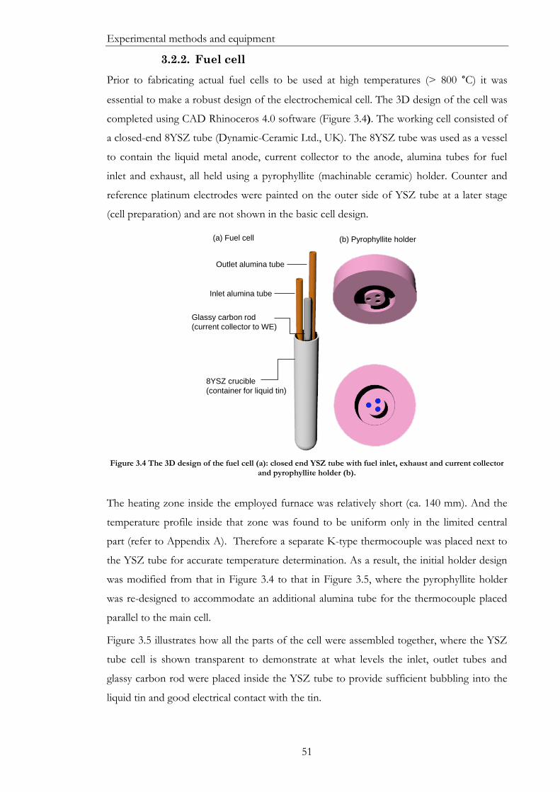
Experimental methods and equipment
51
3.2.2. Fuel cell
Prior to fabricating actual fuel cells to be used at high temperatures (> 800 °C) it was
essential to make a robust design of the electrochemical cell. The 3D design of the cell was
completed using CAD Rhinoceros 4.0 software (Figure 3.4). The working cell consisted of
a closed-end 8YSZ tube (Dynamic-Ceramic Ltd., UK). The 8YSZ tube was used as a vessel
to contain the liquid metal anode, current collector to the anode, alumina tubes for fuel
inlet and exhaust, all held using a pyrophyllite (machinable ceramic) holder. Counter and
reference platinum electrodes were painted on the outer side of YSZ tube at a later stage
(cell preparation) and are not shown in the basic cell design.
Figure 3.4 The 3D design of the fuel cell (a): closed end YSZ tube with fuel inlet, exhaust and current collector and pyrophyllite holder (b).
The heating zone inside the employed furnace was relatively short (ca. 140 mm). And the
temperature profile inside that zone was found to be uniform only in the limited central
part (refer to Appendix A). Therefore a separate K-type thermocouple was placed next to
the YSZ tube for accurate temperature determination. As a result, the initial holder design
was modified from that in Figure 3.4 to that in Figure 3.5, where the pyrophyllite holder
was re-designed to accommodate an additional alumina tube for the thermocouple placed
parallel to the main cell.
Figure 3.5 illustrates how all the parts of the cell were assembled together, where the YSZ
tube cell is shown transparent to demonstrate at what levels the inlet, outlet tubes and
glassy carbon rod were placed inside the YSZ tube to provide sufficient bubbling into the
liquid tin and good electrical contact with the tin.
Inlet alumina tube
Outlet alumina tube
Glassy carbon rod
(current collector to WE)
8YSZ crucible
(container for liquid tin)
(b) Pyrophyllite holder(a) Fuel cell

Experimental methods and equipment
52
Figure 3.5 Updated fuel cell design with YSZ thermocouple placed parallel to the vessel.
3.2.3. Fuel Cell components
Electrolyte
The 8 mol.% yttria-stabilised zirconia (8YSZ) solid electrolyte was chosen due to its ability
to operate at high temperatures and has been shown to have good mechanical strength and
oxygen ion conductivity of 0.13 S cm-1 at 1273 K93.
In order to minimise the ionic resistance, the electrolyte thickness is usually in the range of
50-1000 µm94. As one of the main objectives of this study is to clarify transport of oxidised
species within the liquid anode and not to maximise the fuel cell performance, the
electrolyte thickness chosen for this project was 2000 µm in order to contain the molten
anode (around 25-30 g) safely and securely.
Working electrode (Anode)
Tin was chosen as the anode material for this project due to its low melting point (232° C)
and low vapour pressure. Tin shots of 3 mm dia., 99.99+% (metals basis) (Alfa Aesar, UK)
were used. Once it is melted at ca. 240° C it can be immediately used as a liquid anode.
Alumina tube
for K-type thermocouple
Liquid tin anode
Pyrophyllite holder Inlet and outlet
alumina tube
Current collector
to WE

Experimental methods and equipment
53
Counter and Reference Electrodes
A platinum electrode was chosen as the cathode, as it has high electrical conductivity and
high catalytic activity for the oxygen reduction reaction5. Glass-free Pt ink (4082 Pt Vitr-
Au-Less Conductor, Ferro Electronic Materials) was applied to the outer side of the YSZ
tube followed by its sintering at 1000 °C for 1 hour at a ramping rate of 10 °C per minute.
Pt mesh (10 mm diameter, Goodfellow Cambridge Ltd, UK) with spot welded Pt wires
(0.25 mm diameter, 99.9% Pt, Peak Sensors Ltd) on it were attached with additional ink to
cured platinum and sintered again under the same conditions to achieve good electrical
conductivity across the whole surface.
A reference platinum electrode was placed 10 mm up from the bottom of the YSZ tube
symmetrically around the tube. Attachment of Pt wire to the reference electrode was
difficult to achieve and for that reason a groove was cut 0.5 mm deep around the outside
of the ceramic tube to hold the wire in place. The wire was then twisted and fired at 1000
°C as described above.
Accurate location of the reference electrode is well established for aqueous electrochemical
systems and can be less trivial in the systems with thin solid electrolytes95. Minor errors in
alignment of RE with respect to WE can create significant errors in measurement of the
working electrode96 particularly when rapid changes in potential are involved. In the
present work the geometry of the symmetrical RE was similar to others used typically in
the literature89,94 whereby the RE was adjacent to CE and therefore is considered to be
suitable for this study.
Interconnects
Platinum wires together with Pt mesh were used for the electrical connections necessary
for the operation of the cell. The wires of the mesh itself had a diameter of 0.06 mm and
the mesh was 10-15 mm diameter with an open area of 65%.
A dipping glassy carbon rod was used as an electronic contact to the working electrode
(anode). It provided good electrical connections with the cell with an average electrical
resistance of the glassy carbon rod of 9 Ohms. The employment of glassy carbon as
current collector was one of the achievements of this work. The applied GC rod showed
no deterioration after numerous uses in fuel cell testing (at 800 °C under wide range of
oxygen partial pressures). Unlike other metallic contacts it does not alloy with liquid tin at
800 °C97. Glassy carbon, according to the supplier’s specifications97, shows no wetting by
metallic and ceramic melts and is extremely resistant to thermal shock.

Experimental methods and equipment
54
Fuel cell holder
The cap for the cell is made of Ceramit 14, an industrial name of the machinable mineral –
pyrophyllite which possesses the properties of fired ceramics after heat treatment (firing),
high thermal and mechanical stability, high dielectric strength, etc. Before the firing
pyrophyllite is readily machined (milled, drilled or cut). Machining of a pyrophyllite cylinder
was done using a computer numerical control (CNC) machine, applying precise dimensions
according to the design made in Rhinoceros 4.0 CAD software taking into account volume
contraction of material of around 1.0% on firing. It was then fired at 1400 °C for 1 hour at
ramping rate of 1 °C per minute to achieve high chemical and thermal stability for later use
at high operating temperatures.
The summary of the dimensions of the main fuel cell components with their purpose of
use, chemical composition and commercial suppliers is presented in Table 3.1.
Table 3.1 Description of the parts a fuel cell.
Purpose of use / Material
Dimensions Composition Source
Electrolyte – closed one end 8YSZ tube
19 mm OD, 15 mm ID, LG 210 mm
8 mol. % Y2O3 Dynamic-Ceramic Ltd., UK
Fuel inlet and exhaust – alumina tubes open both ends
4 mm OD, 2mm ID of various lengths
99.7% Al2O3 Multi-Lab Ltd, UK
Liquid metal anode- tin shots
3 mm diameter 99.99+% (metals basis)
Alfa Aesar, UK
Current collection to WE - glassy carbon rod
3 mm OD, LG 250 mm
n/a HTW Hochtemperatur-
Werkstoffe GmbH, Germany
Counter and Reference electrode –platinum ink
n/a Not less than 70% Pt by weight
4082 Pt Vitr-Au-Less Conductor, Ferro Electronic
Materials, US
Interconnects-platinum wire
0.25 mm diameter 99.9% Pt Peak Sensors Ltd, UK
Interconnects-platinum gauze (mesh)
Aperture 0.25 mm; wire diameter 0.06
mm
99.9% Pt Goodfellow Cambridge Ltd., UK
Ceramic holder- pyrophillite cap (Al2O34SiO2H2O)
60 mm OD cylinder with 20 mm height
silica 56.8% Alumina 33.37%
Ferric oxide 0.79% Titanium dioxide
2.42% Magnesium oxide
0.24%
Ceramic Substrates & Components Ltd,
UK
Detection of metallic foam- silica tube
19 mm OD, 15 mm ID, LG 210 mm
SiO2 99.99%
Cambridge Glassblowing Ltd.,
UK

Experimental methods and equipment
55
The ready-assembled fuel cell set-up that was applied in experimental work described in
Chapter 6, 7, 8 and 9 is shown in Figure 3.6.
Figure 3.6 Schematic of a fuel cell used for electrochemical characterisation of LMA SOFC (held in furnace).
3.3. Methodology
Operating conditions used for testing the performance of the LTA SOFC are summarised
in this section. Any additional changes to working conditions with regards to a specific
experiment are listed separately in every chapter of this thesis.
The LTA SOFC was operated in battery and fuel cell modes under flow of inert gas (N2 or
Ar) to eliminate any oxygen leak to the anode and held at temperature >700 °C (typically at
780-800 °C) to reduce ionic resistance of solid electrolyte tube (8YSZ). The system was
heated from room temperature up to the desired temperature (800 °C) at a ramping rate of
5 °C min-1 and likewise when cooled down to room temperature. This condition was
necessary to avoid thermal shock of the components which can induce cracking of
materials used in the rig. Any inevitable leak of oxygen was detected using a potentiometric
sensor that was measuring O2 concentration in the piping leading to the fuel cell.
During electrochemical characterisation of LTA SOFC, electrical connection from the
anode was connected to the working electrode (WE), platinum paint on the outer side of
the 8YSZ tube was connected as the counter electrode (CE) and a platinum ring electrode
was connected as the reference electrode (RE) to the potentiostat.
Pt cathode (CE)Pt reference electrode(RE)
Liquid tin anode(WE)
8YSZ tube
H2/Ar in
H2,H2O/Ar out Glassy carbon rod(anode current collector)
Pyrophyllite cap
Thermocouple Electrical furnace

Experimental methods and equipment
56
3.4. Experimental Methods: electrochemical
techniques
This section briefly describes the theoretical principles of the experimental techniques that
were applied to characterize the performance of the electrochemical system of interest –
LTA SOFC fueled with hydrogen.
The electrochemical characterization techniques were applied to provide details of the
thermodynamic and kinetic aspects of the system based on the applied potentials and
measured currents.
For investigation of the processes occurring in LTA SOFC the following electrochemical
techniques were applied:
Potential sweep methods
Chronoamperometry
Electrochemical Impedance Spectroscopy
Rotating Disc Electrode
Note that the Rotating Disc Electrode (RDE) theory was applied to analyze an inverted
system – Rotating Electrolyte Disc, which differed from standard hydrodynamic aqueous
systems in many aspects (see Chapter 10 for more details).
3.4.1. Potential sweep methods
In potential sweep techniques, such as Linear Sweep Voltammetry (LSV) and Cyclic
Voltammetry (CV) the electrode potential is swept linearly with time between two chosen
values, while current is continuously recorded. Potentials at which species are oxidised or
reduced are registered as current peaks on the voltammogram. The range of a potential
scan is typically chosen so that the initial potential (E1) has no electrochemical activity,
whereas at final potential (E2), the reaction is governed by mass transport98. During LSV
the potential scan stops at a final potential E2, while in CV, when final potential is reached,
the sweep is then reversed back to E1 (or a different potential) and this counts as one cycle.
During CV numerous cycles can be run. The advantage of CV is the ability to identify
redox couples. The cyclic voltammogram produced characterizes the individual reaction
mechanism and kinetic conditions98.
3.4.2. Chronoamperometry / Chronopotentiometry
Chronoamperometry and chronopotentiometry are commonly used electrochemical
techniques that allow the observation of the current-time or voltage-time behavior of
electrochemical system after potential or current step, respectively. In chronoamperometry

Experimental methods and equipment
57
the potential of the electrode is held constant for a certain time period, while current is
determined as a function of time. In the reverse process, constant current is applied
between working and auxiliary electrode, while potential is measured with time between
working and reference electrodes99. In the present work, chronopotentiometry is useful to
study kinetics of an electrochemical cell reaction at a desired voltage. Durability and
stability of the system can also be evaluated using this method.
3.4.3. Electrochemical Impedance Spectroscopy
Electrochemical Impedance Spectroscopy (EIS) is one of the most powerful techniques for
investigation of electrochemical systems as it is capable of separating out different
mechanisms occurring with different time constants43,100–102.
EIS is widely applied for fuel cells diagnosis43 as it provides insight into different
phenomena comprising the overall electrochemical process. The EIS measurements are
typically performed in a large frequency range (usually from high frequency to low
frequency, typically from 10-3 to 107 Hz) at which certain processes with different time-
constants can be observed and distinguished. For instance, electronic conduction and
electrochemical kinetics are relatively faster processes than diffusion (mass-transport)
phenomena and hence can be monitored and evaluated separately via EIS.
In EIS the system under investigation is perturbed with sinusoidal voltage oscillations:
𝑉(𝑡) = 𝑉𝑚𝑠𝑖𝑛 (𝜔𝑡) (3.1)
and the resulting current from the system is recorded accordingly as follows:
𝐼(𝑡) = 𝐼𝑚𝑠𝑖𝑛 (𝜔𝑡 − 𝜑) (3.2)
where 𝜔 is the angular frequency, 𝜑 is the phase difference between voltage and current
signal, 𝑉𝑚 and 𝐼𝑚 are the amplitudes of voltage and current, respectively.
The impedance is defined as the ratio between the output and input signal measured at any
particular frequency. When current perturbations serve as input signal and voltage output is
recorded the obtained impedance, 𝑍(𝑖𝜔), is formulated by:
𝑍(𝑖𝜔) =
𝑈(𝑡)
𝐼(𝑡)= |𝑍|𝑒𝑗𝜑 = 𝑍𝑅𝑒 + 𝑖𝑍𝐼𝑚
(3.3)
where 𝑍𝑅𝑒 and 𝑍𝐼𝑚are the real and imaginary parts of the impedance and 𝑗 = √−1. If
voltage is oscillated and current is measured, the resulting transfer function is called
admittance, 𝑌(𝑖𝜔), and expressed as the inverse function of impedance:
𝑌(𝑖𝜔) =
1
𝑍(𝑖𝜔)= 𝑌𝑅𝑒 + 𝑖𝑌𝐼𝑚
(3.4)

Experimental methods and equipment
58
The impedance data can be represented in a form of a Nyquist plot, where −𝑍𝐼𝑚 is plotted
vs. 𝑍𝑅𝑒 or Bode plot, where magnitude of impedance |𝑍| and phase 𝜑 are shown vs. log (f),
where f is the measuring frequency.
The measured EIS data needs further interpretation using an equivalent electrical circuit
that has an identical response to the measured system of interest and comprises a series of
resistances, capacitances or inductances. The physical meaning of each element in the
circuit should correspond with a particular process that occurs in the overall
electrochemical system. The values calculated for circuit components can provide details
for better understanding of the electrochemical systems100,103.
EIS is a useful tool that allows electrical properties of materials, and their interfaces with
electronically conducting electrodes, to be explored. It has been widely used to investigate
different electrochemical processes: charge transfer of ionic or mixed-ionic conductors,
semiconductors, corrosion processes, investigation of coatings on metals, characterisation
of materials and solid electrolyte as well as solid-state devices104.
It is worth mentioning that interpretation of impedance results is as important as
experimental performance and accuracy. This is not a trivial procedure and depends on
many factors relevant to that particular electrochemical system.
3.4.4. The Rotating Disc Electrode
The Rotating Disc Electrode (RDE) is one of the commonly used hydrodynamic
techniques for analysis of electrochemical systems involving movement of electrode with
respect to the bulk solution. It has been commonly used to study electrode reaction
kinetics105–107.
The RDE theory resulted from the development of mathematical models based on the
solution of the convective-diffusion equation, considering hydrodynamic boundary layer
from the Navier-Stokes equation and other geometric equations107. The velocity profile of a
fluid (bulk solution) near a rotating electrode was developed by von Karman and Cochran
solving the hydrodynamic equations under steady-state conditions99.
The rotation of the electrode is determined via the angular velocity term, 𝜔, which is a
rotation rate parameter:
𝜔 = 2𝜋𝑓 (3.5)
where f - is frequency (number of revolutions per second).
As rotation of the disc increases, the hydrodynamic boundary layer is dragged by the
centrifugal force of the spinning disc away from the centre of the electrode in the radial
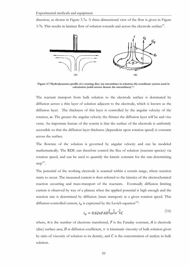
Experimental methods and equipment
59
direction, as shown in Figure 3.7a. A three-dimensional view of the flow is given in Figure
3.7b. This results in laminar flow of solution towards and across the electrode surface99.
Figure 3.7 Hydrodynamics profile of a rotating disc: (a) streamlines in solution; (b) coordinate system used in calculation (solid arrows denote the streamlines)108.
The reactant transport from bulk solution to the electrode surface is dominated by
diffusion across a thin layer of solution adjacent to the electrode, which is known as the
diffusion layer. The thickness of this layer is controlled by the angular velocity of the
rotation, 𝜔. The greater the angular velocity the thinner the diffusion layer will be and vice
versa. An important feature of the system is that the surface of the electrode is uniformly
accessible so that the diffusion layer thickness (dependent upon rotation speed) is constant
across the surface.
The flowrate of the solution is governed by angular velocity and can be modeled
mathematically. The RDE can therefore control the flux of solution (reactant species) via
rotation speed, and can be used to quantify the kinetic constant for the rate-determining
step107.
The potential of the working electrode is scanned within a certain range, where reaction
starts to occur. The measured current is then referred to the kinetics of the electrochemical
reaction occurring and mass-transport of the reactants. Eventually diffusion limiting
current is observed by way of a plateau when the applied potential is high enough and the
reaction rate is determined by diffusion (mass transport) at a given rotation speed. This
diffusion-controlled current, 𝑖𝑑 is expressed by the Levich equation109:
𝑖𝑑 = 0.62𝑛𝐹𝐴𝐷
23𝜔
12ѵ−
16𝐶
(3.6)
where, 𝑛 is the number of electrons transferred, 𝐹 is the Faraday constant, 𝐴 is electrode
(disc) surface area, 𝐷-is diffusion coefficient, is kinematic viscosity of bulk solution given
by ratio of viscosity of solution to its density, and 𝐶 is the concentration of analyte in bulk
solution.

Experimental methods and equipment
60
Levich Analysis
When a series of voltammograms is obtained over the range of different rotation rates
(from lowest to highest), and the rate of reaction is controlled by diffusion of reactant to
the electrode surface, the magnitude of currents in the voltammograms normally increases
with the square root of the rotation rate. The measured limiting currents are usually plotted
vs. the square root of the rotation rate on a graph called a Levich plot. As predicted by the
Levich equation, the limiting current, 𝑖𝑑, increases linearly with square root of the rotation
rate, 𝜔1
2, with the slope of 0.62𝑛𝐹𝐴𝐷2
3ѵ−1
6𝐶. The diffusion coefficient of species in the
bulk solution (electrolyte) can be determined from the slope. The Levich equation is usually
rearranged to the following equation:
1
𝑖𝑑= [
1
0.62𝑛𝐹𝐴𝐷23ѵ−
16𝐶] 𝜔−
12
(3.7)
Koutecky-Levich Analysis
When the rate of reaction is limited by both mass transport and kinetic processes (e.g. at
reaction onset), the RDE technique allows kinetic information (such as standard rate of
reaction) to be separated from mass transport (e.g. diffusion coefficient). The kinetic
current is expressed by109:
𝑖𝑘 = 𝑛𝐹𝐴𝑘𝑓𝐶 (3.8)
where 𝑘𝑓 is the rate constant and is a function of the potential. Then the overall current
measured over the entire potential window is given by the Koutecky-Levich equation109:
1
𝑖=1
𝑖𝑘+1
𝑖𝑑=1
𝑖𝑘+
1
0.62𝑛𝐹𝐴𝐷2
3𝜔1
2ѵ− 1
6𝐶
(3.9)
A plot of reciprocal current versus the reciprocal square root of the angular rotation rate is
called a Koutecki-Levich plot, which yields a straight line with an intercept equal to the
reciprocal of kinetic current. Kinetic current is observed when there are no mass transport
limitations.
3.5. Conclusions
The details of the development of the experimental rig are given. Various types of working
cell were developed and applied in accordance with primary objectives. As such,
symmetrical cells were made for potentiometric and EIS measurements that could provide
information on the ionic conductivity of the YSZ material applied in this project as the

Experimental methods and equipment
61
electrolyte. The fuel cell was developed for testing the performance of LTA SOFC fuelled
with hydrogen. Details of fuel cell components were given.
A brief description of the applied electrochemical characterisation techniques was also
provided. In particular, linear sweep potential, chronoamperometry and electrochemical
impedance spectroscopy were presented. The application of the Rotating Disc Electrode
(RDE) technique normally applied to liquid electrolyte systems is exceptionally important
for the development of the inverted system, Rotating Electrolyte Disc (RED) technique,
appropriate to systems with solid electrolytes.

Preliminary testing
62
4. Preliminary testing This chapter describes the results of preliminary testing of the developed workstation along
with the equipment and materials that are applied for the main experimental work. Testing
of the furnace performance and calibration of the mass flow controllers has been done in
the first instance. This is followed by the testing of conductivity properties of the
electrolyte material chosen for this project, yttria-stabilised zirconia (YSZ). For this work
the symmetrical YSZ cell was applied as a potentiometric oxygen sensor. A good
correlation between experimental data and theoretical response for concentration of
oxygen was found for the applied range of gas flow rates.
Then, ionic conductivity of YSZ was tested, applying a voltage from -1.0 V to 1.0 V and
monitoring a current response. The procedure was repeated with increasing operating
temperature. This resulted in the highest current density at 800 °C and from that it was
confirmed that operation of the fuel cell at around 800 °C was described in order to get
sufficient conductance of electrolyte.
For more accurate and precise calculation of ionic conductivity of YSZ, EIS was applied to
a second symmetrical cell (made of 6 mol.% YSZ). From the high frequency intercept of
the impedance semi-circle, the bulk resistance of the electrolyte was found for the
temperature range from 300 to 1000 °C. It was found that the conductivity trend followed
the well-known Arrhenius relationship and was in close agreement with the literature. Ionic
conductivity of 6 mol.% YSZ was found to be 6.58 × 10⁻² S cm-1 at 1000 °C.
Finally, once all the materials and equipment were tested separately, a measurement of the
ready-assembled LTA SOFC cell was accomplished via OCP measurements with
temperature. Experimentally-determined OCP was in accordance with that predicted by
thermodynamics and demonstrated the readiness of the whole rig and each component for
precise electrochemical characterisation of LTA SOFCs. It also demonstrated the stability
of the glassy carbon rod used as the anode current collector.
Preliminary testing
63
4.1. Introduction
It is essential to test and validate the experimental rig prior any actual electrochemical
characterisation of LTA SOFC. Equipment and materials selected for this project require a
check to ensure operation in a safe and proper manner. Therefore, this chapter describes
the results of preliminary testing of the equipment and materials to be utilised extensively
during the project.
As part of the testing of materials, a potentiometric measurement involving the application
of a symmetrical YSZ cell as potentiometric sensor was performed. To investigate the
overall conductivity of symmetrical cell as a function of applied potential and temperature,
a linear sweep (from -1.0 to 1.0 V vs. air reference) was applied.
The resistance of a solid electrolyte contributes significantly to the overall resistance of an
SOFC. Hence, to investigate and measure ionic conductivity of the electrolyte itself EIS
was applied to a symmetrical 6 mol.% YSZ cell. Resistivity data (from the impedance
diagrams) enables calculation of conductivity at a specified temperature.
The final check of a ready assembled fuel cell and its components is the measurement of
open circuit potential of a cell (OCV). A correct reading (corresponding to
thermodynamics predictions) is an indicator for the proper operation of the whole rig and
individual parts of it.
4.2. Background
4.2.1. Potentiometric measurements of oxygen
concentration using YSZ
One of the common applications of YSZ material is the measurement of oxygen partial
pressure, whereby YSZ is operated as a potentiometric gas sensor110,111. Potentiometric
zirconia sensors can measure oxygen pressure over a wide range from 106 to 10-25 Pa112.
The potentiometric YSZ cell with two metal (typically platinum or silver) electrodes is
typically expressed as follows:
O2 (p2), Pt |O2- conducting electrolyte (YSZ)| Pt, O2 (p1)
The electrode reaction is:
𝑂2 + 4𝑒− ↔ 2𝑂2− (4.1)
Assuming reversibility111 of Reaction (4.1) the cell develops an electromotive force (EMF)
between two metal (Pt) electrodes, which is given by:

Preliminary testing
64
𝐸 = (
𝑅𝑇
𝑛𝐹)∫ 𝑡𝑖𝑜𝑛𝑑(ln 𝑝)
𝑝1
𝑝2
(4.2)
where tion is the transport number of the mobile ion, n is number of electrons transferred
during reaction, p1 and p2 are the partial pressures of oxygen on both sides of the electrolyte
and R, T and F have their usual meaning.
Solid electrolytes generally have low electronic transport numbers, so t ion is close to unity
and hence Equation (4.2) rearranges as follows:
𝐸 =
𝑅𝑇
4𝐹ln (𝑝1𝑝2)
(4.3)
Or:
𝐸 = 2.303
𝑅𝑇
4𝐹 log (
𝑝1𝑝2)
(4.4)
Usually one of the gases in oxygen sensors has known oxygen partial pressure, p2 acting as a
reference gas, while the other is the sample gas with oxygen partial pressure, p1. Therefore,
Equation (4.3) can be applied in the following form:
𝐸 = 𝐸1 + (
𝑅𝑇
4𝐹) ln(𝑝1)
(4.5)
where E1 is a constant of value of −(𝑅𝑇
4𝐹)ln p2.
The reference gases are usually pure oxygen (p2=1 atm) and air (p2= 0.21 atm). In the
experimental set up the reference gas was ambient air, and a mixture of nitrogen and air
was used as the sample gas mixture. The partial pressure of the oxygen was controlled with
mass flow controllers for N2 and air accordingly.
4.2.2. Ionic conductivity of YSZ electrolyte
Section 2.2.7 in the literature review (Chapter 2) provides the details of ionic conductivity
of YSZ material among other solid electrolytes. It also explains the mechanism for transfer
of charged species, which are oxygen ions, O2-. Ionic conductivity of YSZ improves upon
increasing the operating temperature40,113. Therefore it can be expressed with Arrhenius
relationship114 as follows:
𝜎 =
𝜎0𝑇exp (−
𝐸𝑎𝑘𝑇)
(4.6)
where σ is the ionic conductivity, σ0 is the pre-exponential factor, T is the absolute
temperature, Ea is the activation energy, k is Boltzmann’s constant.
Arrhenius relationship predicts linearity between measured conductivity data, ln(σT) and
reciprocal of temperature, 1/T.
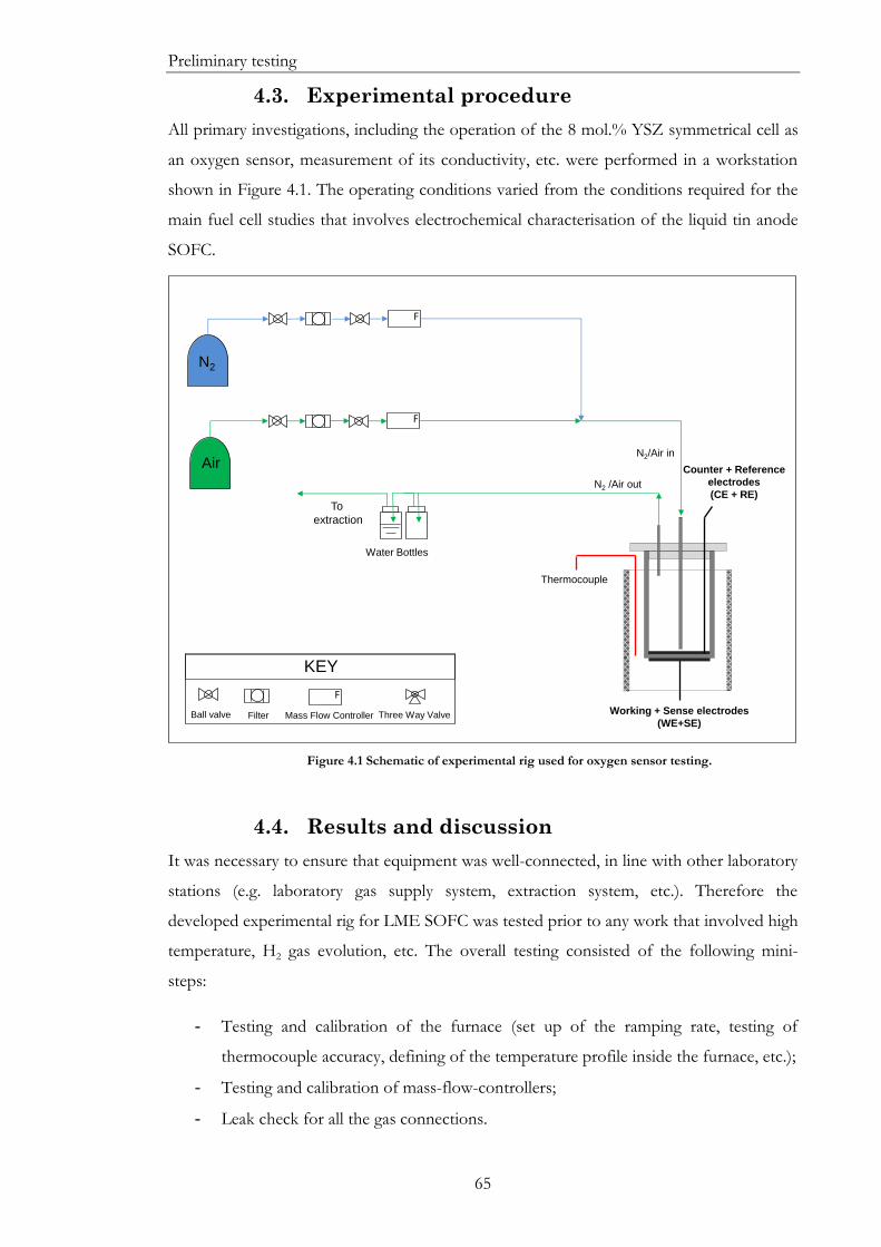
Preliminary testing
65
4.3. Experimental procedure
All primary investigations, including the operation of the 8 mol.% YSZ symmetrical cell as
an oxygen sensor, measurement of its conductivity, etc. were performed in a workstation
shown in Figure 4.1. The operating conditions varied from the conditions required for the
main fuel cell studies that involves electrochemical characterisation of the liquid tin anode
SOFC.
Figure 4.1 Schematic of experimental rig used for oxygen sensor testing.
4.4. Results and discussion
It was necessary to ensure that equipment was well-connected, in line with other laboratory
stations (e.g. laboratory gas supply system, extraction system, etc.). Therefore the
developed experimental rig for LME SOFC was tested prior to any work that involved high
temperature, H2 gas evolution, etc. The overall testing consisted of the following mini-
steps:
- Testing and calibration of the furnace (set up of the ramping rate, testing of
thermocouple accuracy, defining of the temperature profile inside the furnace, etc.);
- Testing and calibration of mass-flow-controllers;
- Leak check for all the gas connections.
N2
Air
F
Water Bottles
To
extraction
F
Ball valve Filter
F
Mass Flow Controller Three Way Valve
KEY
Thermocouple
N2/Air in
N2 /Air out
Working + Sense electrodes
(WE+SE)
Counter + Reference
electrodes
(CE + RE)

Preliminary testing
66
4.4.1. Potentiometric measurements
In the applied experimental set up (Figure 4.2a) the reference gas was ambient air and
hence remained constant, while the sample gas was made of a mixture of nitrogen and air.
Varying the flow rates of nitrogen and air, and hence p1(O2), the EMF across the
symmetrical cell (assuming constant value of p2 of 0.21 atm) was measured and compared
to the value predicted by the Nernst equation (Equation (4.4)). A 10YSZ symmetrical cell
(Figure 4.2b) (full details of the cell were given in Section 3.2.1, Figure 3.3a) was held in the
central part of the electrical furnace and was heated to 700 °C. The flow of a gaseous
mixture (N2+air) supplied to the inner electrode of YSZ was controlled with mass flow-
controllers and varied from (1% air to 100% air). The outer side of the tube was left
exposed to the ambient air with p2(O2) of 0.21 atm. The outer electrode was connected to
the working electrode (WE) terminal, while the inner one – to the counter (CE).
Figure 4.2 Schematic of experimental setup for potentiometric measurements (a) with 10YSZ symmetrical cell (b).
The experimentally measured and calculated EMF data obtained at 700 °C is shown in
Figure 4.3. Overall there is a good agreement between the measured EMF values and
theoretical data calculated using Equation (4.4). Good correlation between experimental
and theoretical data provides confidence that the 10YSZ cell was a reliable and accurate
sensor and the gas flow valves were operating correctly.
Reference gas (air)
WE+ SE
CE/RE
Pt electrodes
10YSZ
symmetrical cell
Pt wire
Pt wire
Sample gas: N2 / Air
(a) (b)

Preliminary testing
67
Figure 4.3 Theoretical (using Equation (4.4)) and experimental EMF developed by the symmetrical cell.
4.4.2. Ionic conductivity of YSZ measured as a function of
applied potential
A relatively quick and simple measurement of solid electrolyte conductivity can be done by
application of a voltage across two electrodes at both sides of the electrolyte and measuring
the current response with step changes in operating temperature.
In order to validate sufficient ionic conductivity of chosen electrolyte material, its
conductivity was tested as a function of applied potential and operating temperature. The
recorded current is then an indication of ionic conductivity of electrolyte. For that the same
symmetrical cell (Figure 4.2b) made of 10YSZ tube and two platinum electrodes described
in details in Section 3.2.1 was held in the electrical furnace.
A linear sweep of voltage between -1.0 V to 1.0 V was applied at temperatures from 500 to
800 °C (connection were as shown in Figure 4.2a). The obtained results in Figure 4.4
demonstrate an increase in 10YSZ conductivity with temperature, as expected from the
literature. At 800 °C there was a substantial increase in current density due to increased
mobility of charges (O2-) in the ceramic (Figure 4.4). The estimated accuracy of measured
currents is ± 50 µA. The obtained data also confirmed the typical operating range for YSZ
(ca. >700 °C for 8-10 mol.% YSZ), as below 700 °C currents were small due to low
conductivity of YSZ.
3.0 3.2 3.4 3.6 3.8 4.0 4.2 4.4-10
0
10
20
30
40
50
60
70
EM
F /
mV
log p(O2) / p(O2) in Pa
Theoretical EMF
Measured EMF

Preliminary testing
68
Figure 4.4 Current – voltage characteristics that includes ionic conductivity of 10YSZ and overpotential on each Pt electrodes.
The above results were complemented and confirmed using the EIS technique as described
below under Section 4.4.3.
4.4.3. Ionic conductivity of YSZ using EIS technique
The next set of experiments was designed to explore the ionic resistivity of the YSZ solid
electrolyte using EIS.101,115–117 As conductivity (reciprocal of resistivity) of solid electrolytes
increases with temperature, the impedance measurements were performed over a wide
range of temperature (from 300 to 1000 °C) with applied potential of 0 V and 10 mV AC
perturbation over the frequency range from 0.01 Hz to 10 kHz. The symmetrical cell, made
of 6YSZ with two Pt electrodes with overall electrode area of 1.30 cm2 and 0.5 cm
thickness, was used. More details are given in the previous Chapter (see Section 3.2.1;
Figure 3.3b). The obtained EIS spectra are shown in Figure 4.5 for the low temperature
range (315 - 422 °C) and in Figure 4.6 - for the high temperature range (722 - 1000 °C).
-1.0 -0.5 0.0 0.5 1.0
-8
-6
-4
-2
0
2
4
6
Curr
ent
density /
mA
cm
-2
Applied Voltage / V
500 0C
600 0C
700 0C
750 0C
800 0C
Applied Voltage / V

Preliminary testing
69
Figure 4.5 Measured EIS data: at 315 - 422 °C frequency sweep: 10 kHz to 0.01Hz, 10 frequencies per decade, Voltage: 0 V, amplitude of oscillations: 10 mV.
Figure 4.6 Measured EIS data at 722, 890 and 1000 °C, frequency sweep: 10 kHz to 0.01Hz, 10 frequencies per decade, Voltage: 0 V, amplitude of oscillations: 10 mV.
The obtained results were interpreted in accordance with commonly used SOFC
impedance models reported by several studies116,118–121. The overall impedance for SOFC
systems comprises the bulk electrolyte impedance (Zb), grain boundary impedance (Zgb) and
electrode impedance (Ze)46. In some studies relevant to impedance scanning of LSM-YSZ
systems it is argued that at least two overlapping arcs should be expected, corresponding
with two processes such as bulk or surface diffusion/adsorption or exchange of oxygen
and transfer of charge118.
The expected bulk and grain boundary arcs can clearly be seen only at 315 °C (Figure 4.5).
The bulk resistance was represented by the first arc at high frequency, while the second arc
at high frequency was attributed to the grain boundary resistance. When the temperature
was increased, the grain boundary arc diminished and it disappeared at significantly higher
0 1x10⁶
2x10⁶
3x10⁶
4x10⁶
5x10⁶
0
1x10⁶
2x10⁶
3x10⁶
4x10⁶
5x10⁶
6x10⁶
0.0 5.0x10⁴
1.0x10⁵
1.5x10⁵
0.0
5.0x10⁴
1.0x10⁵
1.5x10⁵
2.0x10⁵
100 Hz
1 kHz10 kHz
10 Hz
100 Hz
1 kHz10 kHz
100 kHz
10Hz
100 Hz
1 kHz10 kHz
422 C
483 C
315 C
-Im
/ O
hm
.cm
2
Re / Ohm. cm2
100 kHz
Re / Ohm. cm2
-Im
/ O
hm
.cm
2
422 C
483 C
315 C
0 200 400 600 800 1000 1200 1400
0
200
400
10 20 30 40 50 60 70
0
10
20
0.01 Hz
10Hz
100 Hz
1 kHz
from 100 to 0.01 Hz100 kHz
10 kHz
Re / Ohm. cm2
-Im
/ O
hm
.cm
2
890 C
1000 C
100 kHz
10 kHz1 kHz
1 Hz0.1 Hz
Re / Ohm. cm2
-Im
/ O
hm
.cm
2
722 C
890 C
1000 C
1 kHz
100 kHz
10 kHz
100 Hz
10Hz
1 Hz
0.1 Hz
0.01 Hz

Preliminary testing
70
temperatures. Hence, the other complex impedance plots obtained at higher temperatures
(722 - 1000 °C in Figure 4.6) show only one overall depressed arc for all three types of
resistances.
From the obtained impedance plots (movement of semi-circles towards the origin), and in
general reduction in sizes of the arcs, indicates the reduction of the bulk YSZ resistance
with increase of temperature.
High frequency intercept of the impedance arc on the real impedance axis provides the
value of the resistance of electrolyte122,123, ohmic resistance values are listed in Table 4.1.
Table 4.1 Ohmic resistance values for 6 mol. % YSZ symmetrical cell (Pt electrode area of 1.30 cm2) with temperature.
Ωohmic / kΩ T / °C T / K
23.2 316 589 3.94 405 678 2.50 422 695 0.73 483 756 0.65 492 765 0.14 588 861 0.03 722 995 9.34 × 10⁻³ 890 1163 5.87 × 10⁻³ 1000 1273
These data were used to calculate ionic conductivity of 6 mol.% YSZ electrolyte. The
natural logarithm of ionic conductivity of 6YSZ is plotted against reciprocal of temperature
in accordance with Arrhenius equation (Figure 4.7).
Figure 4.7 The electrical conductivity of 6 mol. % YSZ cell as a function of reciprocal absolute temperature.
A straight line was achieved, which confirms the expected Arrhenius behaviour between
measured conductivity and the operating temperature. The slope from Figure 4.7 revealed
the value of activation energy, Ea, for 6 mol.% YSZ sample, which was found to be 0.90
eV. This result is in a good agreement with the one obtained by Arachi et al.122 who
0.0008 0.0010 0.0013 0.0015 0.0018
-6
-4
-2
0
2
4
6
ln (T)=-10281.92T-1+12.67
R2=0.99
6 mol.% YSZ
ln (
T)
/T
in S
cm
-1 K
T-1 / K
-1

Preliminary testing
71
reported an activation energy of 1.0 eV for 6 mol.% YSZ for the similar temperature range
of 350-1000 °C. These results are consistent with a recent study by Zhang et al.113, where
for 8 mol.% YSZ activation energy was reported 0.85 eV in the temperature range of 700-
1000 °C.
The conductivity values for some zirconia-based electrolytes including those measured at
UCL in the present work are summarised in Table 4.2. From the findings it is clear that 6
mol.% YSZ electrolyte has inferior conductivity to 8 mol.% YSZ, and hence the latter is
preferred for electrochemical work, although 6 mol.% YSZ possesses greater toughness.
Therefore in the final design of LTA SOFC, an 8YSZ tube was used.
Table 4.2 Conductivity values of YSZ electrolytes measured and given in the literature.
Source Y2O3 content in ZrO2 σ at 1000 °C / × 10-2 S cm-1
UCL (present work) 6 mol.% 6.58 Yang et al.124 7.5 mol.% 6.67 Arachi et al.122 8 mol.% 14.0 Badwal37 8 mol. % 13.7
4.4.4. Open circuit potential of LTA SOFC
A fuel cell set-up developed previously for LTA SOFC studies (Figure 3.6) was heated
from ambient temperature to 800 °C at the ramping rate of 5 °C per minute. The potential
of working electrode was measured relative to the air reference electrode.
While constantly blowing nitrogen into the cell to maintain inert atmosphere, the open cell
potential developed by the cell was measured with temperature. Figure 4.8 shows a
comparison of theoretically predicted equilibrium potential differences with measured OCP
values for LTA SOFC.
Experimental OCP data for temperatures less than 900 °C was slightly (ca. 40 mV) lower
than theoretical equilibrium potentials. This is possibly due to the fact that saturation of
liquid tin with oxygen had not yet been achieved. On the other hand, at temperature higher
than 900 °C, equilibrium OCP is higher than theoretically possibly caused by oxidation of
the glassy carbon current collector. For comparison, coal oxidation reaction has an
equilibrium potential of ca. 1.02 V70, which is higher than for the Sn-SnO2 equilibrium
potential.

Preliminary testing
72
Figure 4.8 Experimental open circuit potential of the SOFC with a liquid tin anode compared to the theoretical equilibrium potentials for tin oxidation reaction.
Overall, glassy carbon showed itself to be an inert current collector up to 900 °C, which
was suitable for the present study. All electrochemical characterisation of LTA SOFC was
done at 780-800 °C (well below that point), but also normally with a supply of hydrogen
fuel.
In case of constant supply of a fuel which is more reactive than the current collector
material, glassy carbon can be considered as a reliable electronic probe. This situation is
opposite to metallic contacts which tend to alloy with liquid tin at high temperatures and
for that reason were not utilised.
4.5. Conclusions
Preliminary work was essential for validation of the developed workstation with equipment
and material that are going to be applied throughout the project. Potentiometric
measurements involving the application of YSZ tubular cell as an oxygen sensor were
completed. Close agreement between the measured and theoretical EMF data obtained
from a symmetrical cell confirmed that the developed cell was prepared correctly and
operated accordingly.
Ionic conductivity of YSZ material as a function of operating temperature was investigated
using two methods: one varying the applied potential and second, using the EIS technique.
From current-voltage characteristics it was found that the YSZ cell exhibited the highest
conductance at 800 °C in the temperature range considered; hence the temperature range
for operation of LTA SOFC was chosen to be from 750 to 800 °C.
The EIS measurements confirmed the reduction in bulk resistance (attributed to
electrolyte) with increase of temperature. Ionic conductivity of 6YSZ cell was calculated
from the EIS data and was in a good agreement with values reported in the literature. From
400 500 600 700 800 900 1000 11000.0
0.2
0.4
0.6
0.8
1.0
1.2
1.4
Pote
ntial D
iffe
rence / V
Temperature / C
Experimental
Theoretical
Sn(liquid) + O2(gas) SnO
2(solid)

Preliminary testing
73
the obtained result it was decided to utilise 8YSZ material rather than 6YSZ due to its
enhanced conductivity.
The fuel cell developed in the previous chapter was operated in a battery mode (no fuel
supply) and the OCP between the working electrode (anode) and reference electrode was
measured with temperature. Good correlation between measured OCP and potential
difference predicted by thermodynamics of the system was found. A deviation of
experimental OCP from theoretical was found at extremely high temperatures (>900 °C)
which may have been due to oxidation of the current collector.

Experimental optimisation
74
5. Experimental
optimisation This chapter provides analysis of oxygen permeation rates through plastic tubing that was
discovered at early stages of building the LTA SOFC set-up. Parasitic ingress of oxygen
decreased upon reduction in the length of silicone peroxide tubing: later it was reduced via
its complete replacement with hard nylon tubing. Concentration of leaked oxygen was
found to be inversely proportional to the gas flow rate.
A methodology to account for the effect of leaked oxygen into the fuel cell on the overall
fuel cell current was developed. In order to do that the LTA SOFC was operated at -1.1 V
vs. RE when N2 gas was supplied doped with some oxygen pumped in and/or out
electrochemically. The amount of pumped oxygen was consistent with Faraday’s law for
both tubing materials. About 57% of the pumped current (due to oxygen) was attributed to
the change in fuel cell reduction current. This showed that the liquid tin gettered 57% of
the oxygen entering the cell via the supplied carrier gas; this is a surprisingly large fraction
as the gas was in contact with the tin only for a short time (seconds or less). Importantly, it
demonstrated that a substantial fraction of oxygen leaking into the gas supplied to the fuel
cell dissolved in the tin and contributed to currents measured during electrochemical
measurements. Thus, it is vital to ensure minimisation of parasitic oxygen into the carrier
gas.
The developed mechanism not only showed considerable contribution of parasitic oxygen
leaking into tin when LTA SOFC was run at -1.1 V vs. RE, but also indicated how
measured currents could be corrected for parasitic oxygen; such a correction is applied in
experimental chapters of this thesis.
Finally, the values of permeability coefficient for silicone peroxide and nylon tubing are
determined and compared to literature values. Replacement of silicone peroxide tubing
with nylon should have resulted in virtually zero permeability. The apparent permeability
coefficient of 1.3×10⁻¹¹ cm2 s-1 Pa-1 measured for nylon tubing indicated that permeation
occurred through the joints and connectors, where short sections of silicone peroxide
tubing were used for making connections.
.

Experimental optimisation
75
5.1. Introduction
One of the challenges in the operation of LMA SOFCs is to maintain the metal anode in
an inert atmosphere. In order to flush the operating system and prevent any leak of oxygen
to the anode the carrier gases N2 or Ar were typically applied18,21,64,66,70.
Electrochemical oxidation of liquid metal to metal oxide is one half reaction of the whole
mechanism of the fuel cell, and therefore the level of oxygen present in the inert carrier gas
should, if possible, be reduced virtually to zero in order to minimise any chemical oxidation
of the anode.
At early stages of this project when the experimental rig was under construction using
various types of plastic tubing, significant amounts of oxygen were detected in the carrier
gas (nitrogen) after traversing the tubing.
Therefore, the aim of the work presented in this chapter is to quantify permeation of
oxygen through the silicone peroxide tubing incorporated initially (and nylon tubing used
subsequently). Traces of oxygen in the system were detected even after replacement of
most of the soft tubing with hard impervious tubing. A methodology was developed
whereby oxygen was electrochemically pumped in or out to the carrier gas supplied to the
fuel cell. The methodology enabled investigation of the effect of pumped/parasitic oxygen
on the fuel cell current.
5.2. Background
Transport of gases in polymer membranes has been studied widely over the past 150
years125–127. The gas transport theory in synthetic polymeric membranes is dependent upon
the morphology of the polymer and as such there are two main types of polymers for
consideration: rubbery and glassy polymers125.
The focus of this chapter is permeation through rubbery polymers (in particular silicone
rubber). Permeation according to the ‘solution-diffusion model’125 is governed by two
processes: sorption (conforming to Henry’s law solubility) and diffusion (governed by
Fick’s law of diffusion).
Combining sorption and diffusion, the steady state permeation rate (or flux) through a
membrane of thickness τ is expressed as follows:
𝐽 =
𝐷𝑆∆𝑝
𝜏
(5.1)
where D is the diffusion coefficient, S the absorption coefficient, and Δp the pressure
difference.

Experimental optimisation
76
Assuming that diffusion and solubility coefficients are independent of concentration of a
gas in a membrane, the permeation flux is expressed as follows:
𝐽 =
𝑃∆𝑝
𝜏
(5.2)
And the permeability coefficient is then:
𝑃 = 𝐷𝑆 =
𝐽𝜏
∆𝑝
(5.3)
Apart from solubility and diffusivity of a small molecule in the polymer, other factors that
affect permeability of a polymer are chain packing and side group complexity, polarity,
orientation, fillers, humidity and plasticization128.
Permeability of a membrane is used to characterise the permeation rate of a membrane and
is typically expressed as follows:
𝑃 =
𝑉𝜏
𝐴𝑡∆𝑝
(5.4)
where P is permeability for a given temperature, V is volume of gas which penetrates
through a membrane, τ is thickness of a membrane, A is area of a membrane, t is time and
Δp is partial pressure difference across the membrane.
Analysis of oxygen permeation through plastic tubing based upon ‘solution-diffusion’
theory in the present work is shown below. As all the experiments were run at ambient
temperature (25 °C) and pressure (1 bar) and with the same permeant, namely oxygen, the
dependence of permeability, solubility upon the gas type, temperature and pressure are not
considered in the theoretical treatment of the results, which is shown below.
5.2.1. Theoretical analysis of oxygen permeation with the
effect of pumping current
Based on studies of transport of gases and vapours in polymers127, the following theoretical
framework has been developed for the analysis of permeation rate of air (oxygen) through
silicone peroxide tubing with a constant flow of nitrogen through it.
Consider permeation through plastic tubing (silicone peroxide), with length l, from air
surrounding the tube to N2 with O2 content close to zero (Figure 5.1). Let the gas
(nitrogen) input to the tube have O2 content of ppm (from gas cylinder specification)
and the output, 𝑐 ppm. Note that 1 ppm of O2 is parts per million by moles but also by
volume.

Experimental optimisation
77
Figure 5.1 Schematic of the oxygen permeation through silicone peroxide tubing (containing N2) with electrochemically pumped oxygen.
Permeation rate of oxygen through plastic tubing is shown as Y cm3 s-1, for the total length
of tubing, l, where X ml s-1 is the flow rate of nitrogen gas and l is the total length of tubing
and pumped current, I in A. The electrochemically pumped oxygen is treated below.
In order to quantify the amount of injected oxygen via the oxygen pump, the following
reaction with four electrons transfer is considered:
2𝑂2− ↔ 𝑂2 + 4𝑒− (5.5)
So the rate of oxygen pumping is 𝐼
4𝐹 mole s-1 of oxygen, which is 𝐼
4𝐹(22.4 × 10³) cm3 s-1,
where F is the Faraday constant, 0.965 × 10⁵ C mol-1, and hence the volume of oxygen
pumped (at STP) is equal to:
𝐼 ×(22.4×10³)
4×0.965 × 105 = 0.058 𝐼 cm3 s-1
For a nitrogen (or argon) flow rate of X ml s-1, the following equation may be written:
𝑐 =
106
𝑋(𝑌 + 0.058 𝐼) +
(5.6)
where 𝑐 is the concentration of oxygen in ppm.
For constant or zero current, a plot of oxygen concentration, 𝑐 vs. inverse of gas flow rate,
X-1 should be a straight line with a slope of 106Y, and intercept, .
In case when additional oxygen is pumped in, for a fixed flow rate of nitrogen X, the plot
of oxygen concentration, 𝑐 in ppm vs. pumped current, I, should result in intercept (units:
ppm):
𝑖𝑛𝑡𝑒𝑟𝑐𝑒𝑝𝑡 = +106
𝑋𝑌
(5.7)
and slope (units: ppm μA-1)
𝑠𝑙𝑜𝑝𝑒 =
0.0580
𝑋
(5.8)
Permeation rate of O2,
Concentration of O2,
N2 in
Total length of tubing,
cm3 s-1
(ml s-1) with
cm
ppm O2
N2 out
, ppm
Electrochemically pumped oxygen, cm3 s-1

Experimental optimisation
78
5.2.2. Calculation of oxygen concentration using
potentiometric sensor
Oxygen concentration is determined from the EMF measured between two Pt electrodes
located on each side of a YSZ cell, which is governed by the Nernst Equation as follows
(see Chapter 4 for more details):
𝐸 =
𝑅𝑇
4𝐹 ln (
𝑝𝑂2 𝑠𝑎𝑚𝑝𝑙𝑒𝑝𝑂2 𝑟𝑒𝑓
) (5.9)
where R is universal gas constant, T is absolute temperature, 𝑝𝑂2 𝑟𝑒𝑓 is partial pressure of
oxygen in dry, clean air (0.21 atm) and 𝑝𝑂2 𝑠𝑎𝑚𝑝𝑙𝑒 - is the partial pressure of oxygen to be
measured.
Assuming 210,000 ppm of O2 in the ambient air (reference gas), Equation (5.9) could be
written as follows:
𝐸 = 2.303
𝑅𝑇
4𝐹log (
𝑐𝑎𝑚𝑝𝑙𝑒
210,000 )
(5.10)
where 𝑐𝑎𝑚𝑝𝑙𝑒 is unknown oxygen concentration (in ppm) in the sample gas.
Equation (5.10) allows the determination of an unknown oxygen concentration (in ppm) in
the sample gas, 𝑐𝑎𝑚𝑝𝑙𝑒 from the measurement of EMF between two electrodes, E.
This chapter presents an investigation of oxygen permeation through silicone peroxide and
nylon tubing. It also provides the methodology for doping of carrier gas with oxygen using
an electrochemical pump. The effect of oxygen pumped in and out on the overall fuel cell
current is also presented.
5.3. Experimental procedure
In the present chapter all experimental work entails operation of the LTA SOFC cell at an
operating temperature of 760-780 °C. Experimental set-up and compartments of the
working cell were similar to the ones described in Chapter 3. However, some modifications
to the original set-up were made to fulfil the requirements for the practical work on the
oxygen diffusion through plastic tubing as well as pumping of oxygen in and out of carrier
gas prior to its entering the liquid tin electrode fuel cell. The carrier gas used in the
measurements was zero grade (6 ppm O2) nitrogen (BOC, UK).
The most important pieces of equipment that were added to the main set-up:
potentiometric oxygen sensor (Kent Industrial Measurements, UK), oxygen pump (made
of 10YSZ symmetrical cell (closed at one end) with Pt electrode on inner and outer side of
the tube) and electrical furnace to heat up both sensor and pump (Figure 5.2). The outer

Experimental optimisation
79
diameter of the 10YSZ tube was 10 mm with wall thickness of 1 mm and overall length of
120 mm. Platinum ink (4082 Pt Vitr-Au-Less Conductor, Ferro Electronic Materials, USA)
for electrodes was painted on the inner and outer sides of the YSZ tube and sintered at
1000 oC for 2 hours (ramp rate of 10 °C per minute). Platinum wires were attached to each
electrode prior to sintering, for electrical connections.
Figure 5.2 Electrical furnace for heating oxygen sensor and oxygen pump (closer look) in the overall set-up (a); oxygen sensor (b); oxygen pump (10YSZ symmetrical cell (closed at one end) with two Pt electrodes and Pt
wires) (c).
During the practical work two types of tubing were used. During the early stages, 1/4’’
(6.35 mm) OD, 1/8’’ (3.18 mm) ID flexible vinyl (PVC) tubing (Swagelok, UK) suitable for
operation from -40 to 73 °C was used together with 4 mm OD, 2 mm ID silicone peroxide
tubing (VWR International Ltd., UK). At later stages, vinyl and silicone peroxide tubing
were replaced by hard, lightweight, flexible nylon tubing of two sizes 1/4 (6.35 mm) OD
and 1/8’’ (3.18 mm) OD (Swagelok, UK) suitable for operation from -40 to 93 °C. All
types of tubing employed in this chapter are listed in Table 5.1.
(a)
(b) (c)

Experimental optimisation
80
Table 5.1 Details of all the tubing employed in experimental work.
Name of the tubing
Material Dimensions Supplier
Vinyl Polyvinyl chloride (PVC) - (C2H3Cl)n
1/4’’ (6.35 mm) OD and 1/8’’ (3.18 mm) ID
Swagelok, UK
Silicone peroxide Basic elastomer – silicone; catalyst/filler - peroxide
4mm OD and 2 mm ID VWR International Ltd., UK
Nylon Nylon 1/4’’ (6.35 mm) OD, thickness 1.0 mm
Swagelok, UK
Nylon Nylon 1/8’’ (3.18 mm) OD, thickness 0.5 mm
Swagelok, UK
An electronic circuit connected to the 10YSZ cell (oxygen pump) was inserted into the
overall set-up to drive the pump. An electronic circuit was built specifically to be used with
the oxygen pump (Figure 5.3), where the voltage (5 V) from the power supply unit was
divided using four 1 k resistors connected in series, which provided 1.25 V across each of
the resistors (Figure 5.3a). The complete circuit consisting of ammeter, voltmeter and
variable resistor (up to 1 MΩ) together with the oxygen pump is shown in Figure 5.3b.
Figure 5.3 Electronic circuit with 10YSZ cell served to pump oxygen in and out of nitrogen flow (a); schematic of the operation of the oxygen pump using the electronic circuit (b).
A schematic of the experimental rig used in this work is shown in Figure 5.4a with detailed
representation of the oxygen sensor and oxygen pump operable with in-house built
electronic circuit, shown in Figure 5.4b. The flow of nitrogen was supplied to the oxygen
pump (to pump oxygen in or out) followed by the oxygen sensor and then entered the fuel
cell (Figure 5.4c) held at operating temperature by an electric furnace. Both oxygen sensor
and oxygen pump were held inside a second electrical furnace (Kent Industrial
Measurements, UK, 100 W), which was powered by two power supply units (PSU)
connected in series (to achieve the required 12 V).
(a)
A
YSZ cellOuter electrode Inner electrode
5 V
R
R R
R
1MΩ
1 kΩN2+ 5 ppm O2
V
A
e-e-
0.21 atm O2
(b)
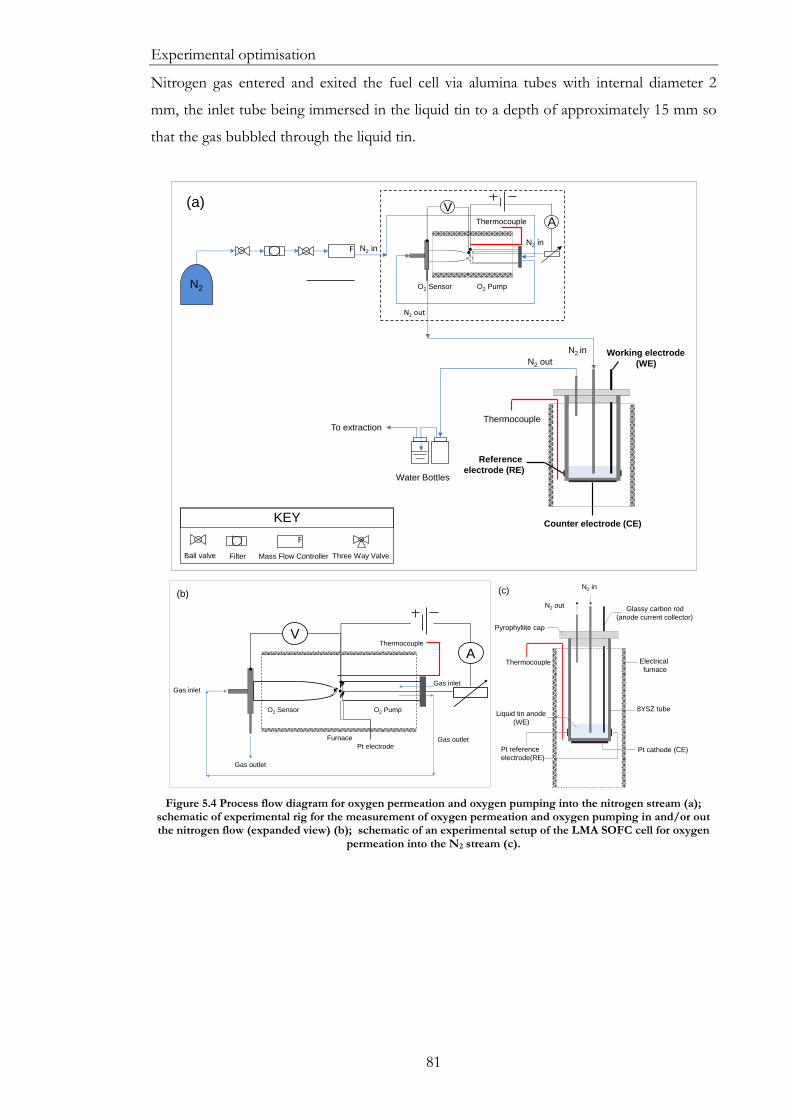
Experimental optimisation
81
Nitrogen gas entered and exited the fuel cell via alumina tubes with internal diameter 2
mm, the inlet tube being immersed in the liquid tin to a depth of approximately 15 mm so
that the gas bubbled through the liquid tin.
Figure 5.4 Process flow diagram for oxygen permeation and oxygen pumping into the nitrogen stream (a); schematic of experimental rig for the measurement of oxygen permeation and oxygen pumping in and/or out the nitrogen flow (expanded view) (b); schematic of an experimental setup of the LMA SOFC cell for oxygen
permeation into the N2 stream (c).
N2
Water Bottles
To extraction
F
Ball valve Filter
F
Mass Flow Controller Three Way Valve
KEY
Thermocouple
Working electrode
(WE)
Reference
electrode (RE)
Counter electrode (CE)
N2 in
N2 out
N2 in
N2 out
O2 Sensor O2 Pump
Thermocouple
N2 in
VA
(a)
V
Gas outlet
Gas inlet
Furnace
Pt electrode
A
Gas inlet
Gas outlet
Thermocouple
O2 Sensor O2 Pump
(b)
Pt cathode (CE)Pt reference
electrode(RE)
Liquid tin anode
(WE)
8YSZ tube
N2 in
N2 outGlassy carbon rod
(anode current collector)
Pyrophyllite cap
Thermocouple Electrical
furnace
(c)

Experimental optimisation
82
5.4. Results and discussion
5.4.1. Permeation of oxygen through silicone peroxide and
nylon tubing
Early measurements were carried out using the set-up shown in Figure 5.4. Oxygen
concentration was measured using a potentiometric sensor in the N2 line at a flow rate of
1.67 ml s-1 and resulted in ca. 500 ppm of O2 exceeding the O2 concentration in the N2
cylinder (6 ppm according to specification) by 100 times. Reducing the flow rate down to
0.83 ml s-1 resulted in an almost doubled initial O2 concentration (1045 ppm).
As a result the permeation rate of oxygen through silicone peroxide tubing was explored as
a function of flow rate of supplied gas (nitrogen). The EMF (together with sensor
temperature) was measured at 1.67, 0.83 and 0.33 ml s-1 flow rates before and after
reduction in length of silicone peroxide tubing from 88 cm down to 8 cm.
Subsequently, in order to reduce parasitic leakage of oxygen through soft silicone peroxide
tubing most of the soft tubing was replaced with less permeable nylon tubing.
A plot of the concentration of leaked oxygen (into N2 flow) versus the reciprocal of flow
rate is shown in Figure 5.5 for the original and reduced length of silicone peroxide tubing,
88 and 8 cm respectively, as well as for nylon tubing.
Figure 5.5 Concentration of oxygen diffused through silicone peroxide tubing of 88 and 8 cm and nylon tubing (8 cm) vs. inverse of the gas flow rate.
The obtained data (Figure 5.5) resulted in the straight lines, which provides confidence that
the measurement of concentration using the potentiometric oxygen sensor was reliable and
accurate. An indicated earlier, inverse proportionality between oxygen concentration and
the flow rate of nitrogen predicted by the theory was confirmed (Section 5.2.1).
0 2 4 6 8 10
0
1
2
3
4
5
6
7
8
c
c
l=8 cm; nylon tubing
l=8 cm; silicone peroxide tubing
l=88 cm; silicone peroxide tubing
Reciprocal of the gas flow rate / s ml-1
Concentr
ation o
f O
2 /
10
3 p
pm
=846(X)-1- 29.1
=103(X)-1-1.37
=35.2(X)-1-11.9
c

Experimental optimisation
83
From the above theory it is expected that oxygen permeation rate should be proportional
to the length of tubing, l. The difference in the slopes (almost 8 times) in Figure 5.5 upon
reduction of length of tubing from 88 cm down to 8 cm serves as strong evidence to that,
as no other parameter was changed during that experiment. Despite that reduction, precise
ratio of the slopes according to theory should be 11:1 rather than 8:1. A possible
explanation is that some leakage of oxygen was also occurring through the joints.
Replacement of the soft by hard tubing resulted in significant reduction of oxygen
permeation rates by a factor 2-3 for similar length of hard (nylon) and soft (silicone
peroxide) tubing.
The oxygen permeation was investigated by application of the oxygen pump and electronic
circuit illustrated in Figure 5.3 whereby oxygen was electrochemically injected and/or
removed from the N2 flow. Figure 5.6 shows the measured oxygen concentration vs.
pumped current for silicone peroxide (reduced in length) and nylon tubing.
Figure 5.6 Concentration of O2 vs. pumped current with N2 flow rate of 1.67, 0.83 and 0.33 ml s-1 using 8 cm silicone peroxide tubing (a) and hard tubing (b).
Plotting the intercepts from Figure 5.6 vs. the reciprocal of the flow rate resulted in straight
lines for both silicone peroxide and nylon tubing. The obtained lines confirm the inverse
proportionality between the experimentally measured intercepts (i.e. concentration of O2 at
zero pumped current) and the gas flow rate. This once again confirms that the
concentration of oxygen is inversely proportional to flow rate as presented above in Figure
5.5., while the leakage rate was constant.
-1000 -500 0 500 1000
0
100
200
300
400
500
600
(a)
Co
nce
ntr
atio
n o
f O
2 /
pp
m
0.33 ml s-1
0.83 ml s-1
1.67 ml s-1
Pumped current / A
-500 0 500 1000 1500 2000 2500 3000 3500
0
200
400
600
800
1000
1200
Pumped current / A(b)
Concentr
ation o
f O
2 /
ppm
0.33 ml s-1
0.83 ml s-1
1.67 ml s-1

Experimental optimisation
84
Figure 5.7 Intercepts obtained from Figure 5.6 against reciprocal of the flow rate for silicone peroxide and nylon tubing.
The positive effect from replacement of silicone peroxide tubing with less permeable nylon
tubing was evident from the difference of two slopes of straight lines (i.e. 102 vs. 80.0 ppm
ml s-1). This would indicate the reduction in diffused O2 concentration with nylon tubing
compared to silicone peroxide at no pumping of additional oxygen.
Close agreement in the slopes obtained from Figure 5.7 and Figure 5.5 (102 and 103 ppm
ml s-1) is additional confirmation that same amount of oxygen was diffusing through 8 cm
long silicone peroxide tubing during two separate measurements. This indicates consistency
in the results obtained using different experimental methods.
In Figure 5.6, all the lines for each flow rate apart from those at 0.33 ml s-1 are parallel (the
slopes are in a good agreement), which confirms that the amount of oxygen pumped was
consistent with Faraday’s law shown in Equation (5.8) with both tubing materials. The
following figure (Figure 5.8) provides additional confirmation to that. Two values with
both materials obtained with slowest flow rate 0.33 ml s-1 were not aligned with theoretical
line. This could be due to some minor leak of oxygen at the joints, which was less
influential at higher flow rates (1.67 and 0.83 ml s-1).
Overall the obtained results with two materials confirmed that replacement of silicone
peroxide tubing with nylon tubing led to a significant reduction of O2 levels in the nitrogen
flow.
0.5 1.0 1.5 2.0 2.5 3.0
0
50
100
150
200
250
300
350 nylon
silicone peroxide
linear fit
linear fit
Inte
rcept /
ppm
Reciprocal of the gas flow rate / s ml-1

Experimental optimisation
85
Figure 5.8 Relationship between theoretical and measured injection rate of oxygen and gas flow rate with both silicone peroxide and nylon tubing.
5.4.2. Oxygen pumping in and out of liquid tin anode
during cathodic reduction of oxygen in LTA SOFCs
Replacement of silicone peroxide tubing with nylon reduced the amount of oxygen that
leaked into the nitrogen line. Having reduced the levels of oxygen the effect of the
remaining parasitic oxygen fed into the fuel cell during the electrochemical measurements
in LTA SOFC was investigated.
The simplest reaction in LTA SOFC where parasitic leak of O2 could be studied was
cathodic reduction of oxygen (dissolved in tin) at some negative potential (with respect to
Sn/SnO2 redox couple). While measuring the current response from a fuel cell, some
oxygen was added and/or removed using the oxygen pump. This enabled the effect of
pumped oxygen on the overall fuel cell current to be explored.
The LTA SOFC cell (Figure 3.6) was heated in a vertical furnace to 761 °C under flow of
1.6 ml s-1 of gaseous mixture of dry H2 and N2 (4: 96). The potential of the tin electrode
was held at -1.1 V vs. RE and the current response was monitored with time, while O2 was
pumped into or out of the nitrogen stream supplied to the fuel cell (Figure 5.9). The
estimated accuracy of measured currents is ± 50 µA.
0 1 2 3 4
0.00
0.05
0.10
0.15
0.20
0.25
Reciprocal of the gas flow rate / s ml-1
Slo
pe
s /
pp
m (
mA
)-1
nylon tubing (8 cm)
silicone peroxide tubing (8 cm)
theoretical line

Experimental optimisation
86
Figure 5.9 The effect of pumped in and pumped out current on cathodic current measured at -1.1 V vs. RE under flow of 1.6 ml s-1 of gaseous mixture of dry H2 and N2 (4: 96).
One of the limitations of the experiment was removal of greater amount of O2 (the
pumping out current could not exceed 75 μA). Removal of more oxygen was possible only
if higher voltage across the electrodes of the pump had been applied. That, however, could
potentially induce electronic conductivity of ZrO2 in the 10YSZ tube, which was not
desirable129 as Faraday’s law does not apply for current carried electronically.
Figure 5.10a shows the linearity between pumped current and steady cathodic current at
each O2 injection rate into the N2 flow. Increase in pumped current resulted in higher in
magnitude fuel cell current, as more oxygen was supplied to the fuel cell to be reduced at
liquid tin/ YSZ interface at -1.1 V. The obtained slope of ca. 0.57 indicates that around
57% of injected current had translated into the overall fuel cell current, and that the
remained of pumped oxygen did not stay in the tin but was carried from the cell in the
carrier gas. This is an interesting and important result because it shows that although the
transit time of the bubbles was very short (the time it took for them to rise through 15 mm
of tin) more than half of the oxygen was extracted into the tin. Extraction of the oxygen
into the tin can only takes place at the interface between the bubble and the tin. So clearly
the time constant for diffusion and oxygen gettering within the dimensions of the bubbles
is short. It would also suggest that oxygen reaching the interface dissolves or reacts with tin
rapidly. This has implications regarding water reduction and will be recalled in Chapter 9.
The intercept of ca. 0.89 mA in Figure 5.10a was the value of the steady fuel cell (cathodic)
current at zero pumping current and was due to the parasitic oxygen content of the carrier
0 2 4 6 8 10 12 14
-18
-16
-14
-12
-10
-8
-6
-4
-2
0
Time / 103 s
Cu
rre
nt
/ m
A
cathodic current at -1.1 V vs. RE
2 4 6 8 10 12 14
-1.6
-1.2
-0.8
-0.4
75A
pum
pin
g in 996
A
pum
pin
g in 4
00
A
pum
pin
g in 1
.31 m
A
pum
pin
g in 1
.27 m
A
Time / 103 s
Cu
rre
nt
/ m
A
current affected by pumping
steady current at no pumping
pumping out

Experimental optimisation
87
gas. The amount of pumped oxygen had a primary effect on overall fuel cell current, which
is shown in Figure 5.10b. One would expect that when zero oxygen was present in the
system, the fuel cell current would also be zero. The intercept of -0.31 mA can be
accounted as not significant as it was within the standard deviation of measured
concentration.
Figure 5.10 Steady cathodic current (a) vs. pumped current and (b) vs. O2 concentration with total flow rate of 1.6 ml s-1.
The plot of O2 concentration versus the pumped current (Figure 5.11) resulted in a straight
line with a slope of 50 ppm O2 per 1 mA of pumped current. The intercept of 51 ppm
indicated that this amount of O2 was present in the tubing (when no O2 was injected or
removed electrochemically via the pump).
Figure 5.11 Concentration of O2 vs. pumped current at total flow rate of 1.6 ml s-1.
It is possible to compare the determined slope with the slope dictated by Faraday’s law.
The volume of oxygen pumped in ml s-1 per 1 mA can be expressed as follows:
𝑑
𝑑𝑡=𝐼
4𝐹
(5.11)
This is equivalent to a flow of oxygen in ml s-1:
40 50 60 70 80 90 100 110 120
-1.6
-1.4
-1.2
-1.0
-0.8(b)
Ste
ad
y c
ath
od
ic c
urr
en
t /
mA
O2 concentration / ppm
-0.2 0.0 0.2 0.4 0.6 0.8 1.0 1.2 1.4
-1.6
-1.4
-1.2
-1.0
-0.8
Ste
ady c
ath
odic
curr
ent
/ m
A
Pumped current / mA
(a)
-0.2 0.0 0.2 0.4 0.6 0.8 1.0 1.2 1.4
40
50
60
70
80
90
100
110
120
O2 c
oncentr
ation /
ppm
Pumped current / mA

Experimental optimisation
88
𝐼
4𝐹22.4 × 10³
(5.12)
Injecting this into a N2 flow of 1.6 ml s-1 results in oxygen concentration of 22.4×103𝐼×106
(1.6)4𝐹
ppm or 22.4×10⁶
6.4𝐹ppm mA-1, i.e. 36.3 ppm (mA)-1 compared to experimentally found 50.0
ppm per 1 mA (Figure 5.11). The discrepancy between the two values may indicate loss of
N2 before it flows through the pump because this would raise the O2 concentration in the
gas.
Overall the applied methodology when oxygen is pumped in or out of the fuel cell during
chronoamperometric measurements was important. Using this technique, any inevitable
leak of oxygen into the fuel cell can be taken into account and be separated from the
overall fuel cell current.
Prior to any electrochemical measurements, steady oxygen reduction current should be
measured when LTA SOFC is operated at some negative (with respect to OCV)
overvoltage (say -1.1 V) and supplied only with carrier gas (N2 typically). Then if the fuel
cell is operated at positive overvoltage, the oxygen reduction current should be added to
the overall anodic current. On the contrary, if LMA SOFC is operated cathodically then the
oxygen reduction current should be subtracted from the overall current. This technique for
addressing inevitable leak of oxygen into the system is applied in further experimental
chapters of this thesis.
5.4.3. Determination of permeability coefficient for plastic
tubing
Calculation of permeability coefficient for silicone peroxide tubing, P can be found using
the equation (derived in Appendix B) as follows:
𝑃 =𝑌 𝑙𝑛(
𝑟1𝑟2⁄ )
21, 000 (2𝜋𝑙)
(5.13)
where Y is permeation rate of oxygen, cm3 s-1, r1 and r2 are the external and internal
diameters of the tubing, l is total length of tubing, 21,000 is the concentration of oxygen
outside the tubing/ Pa.
Recalling Figure 5.5 where for silicone tubing of total length of 88 cm, the slope of 846
ppm ml s-1 was obtained, which according to Equation (5.6) is 106Y. Thus Y=846×10-6 cm3
s-1. From dimensions of silicone peroxide tubing given in Table 5.1, the value of ln(r1/r2)
can be found. Substituting all into Equation (5.13) obtain:
𝑃 =846×10−6× 0.693
0.21×105×2𝜋×88= 5.1 × 10⁻¹¹ cm2 s-1 Pa-1 .

Experimental optimisation
89
Applying the analysis for nylon tubing, the permeability coefficient was found to be
1.3×10⁻¹¹ cm2 s-1 Pa-1, which about 4 times smaller than silicone tubing. This value was still
higher than expected, as according to its technical specification is considered to be
impermeable to oxygen. A possible explanation for the apparently elevated value for the
nylon tubing is that there remained leakage via “soft plastic” connectors and joints, where
it was not possible to connect directly between the metal fittings and the nylon tubing.
The obtained values for both silicone peroxide and nylon tubing in the existing set-up was
higher than values for other polymers (see comparative Table 5.2). The actual permeability
for nylon should be lower than most of the polymers, albeit the apparent permeability
(measured taking into consideration all plastic connectors and joints) was relatively high.
Table 5.2Permeability in polymers at 25 °C for oxygen gas128.
Polymer P/10-13 cm2 s-1 Pa-1 at 25 °C
Polyethylene (LDPE) 2.2 Poly(ethyl methacrylate) 0.9 Poly (ethylene terephthalate) 0.04 Poly (vinylidene chloride) 0.004 UCL (present work)–silicone peroxide 510 UCL (present work)- nylon (polyamide) 130
So the tubing applied in early stages of this project was very permeable to oxygen
compared with all other plastics shown above. And therefore was considered not a good
plastic to be used for piping “oxygen-free” gases. Notwithstanding that some soft
connectors and joints remained in the plumbing, the nylon tubing that replaced silicone
peroxide tubing had significantly reduced permeation to oxygen compared to silicone
peroxide.
5.5. Conclusion
Parasitic leakage of oxygen into the LTA SOFC cell was a serious problem that needed
urgent solution prior to any accurate electrochemical measurement in LTA SOFC.
Several improvements made to the experimental rig enabled a reduction to be made to
levels of O2 in the nitrogen stream from 1045 ppm (initially) down to 50 ppm (finally) with
1.67 ml s-1 flow rate of N2 in both cases. This was achieved by firstly reducing the length of
silicone peroxide tubing from 88 to 8 cm, and secondly by replacing most of the silicone
peroxide tubing with less permeable nylon tubing.
Agreement between experimentally-measured permeation rate of oxygen through various
tubing (silicone peroxide and nylon) and theoretical prediction (based upon Faraday’s law)
provides confidence in accurate and reliable operation of both the potentiometric sensor
and the electrochemical pump.

Experimental optimisation
90
Using the oxygen pump and electrical circuit it was possible to remove O2 and maintain its
concentration in N2 flow at acceptable levels. The technology developed to account the
influence of parasitic oxygen on overall fuel cell performance showed that 57% of pumped
oxygen current was translated to the overall fuel cell current, when LTA SOFC was
operated at -1.1 V vs. RE and fed with dry N2. That methodology considers some parasitic
oxygen to be inevitable. It is shown that it is possible to correct for its contribution to fuel
cell anodic or cathodic current measurements and this is done in the remaining chapters of
this thesis.
Finally permeability coefficient for both types of tubing was calculated as 5.1×10⁻¹¹ and
1.3×10⁻¹¹ cm2 s-1 Pa-1 for silicone peroxide and nylon tubing, respectively. The two values
were higher than for other polymers. However, it is considered that the apparently high
value measured for nylon was due to the use of short length of soft tubing to enable pipes
to be fitted readily to metal connectors.

Proposed mechanisms for oxidation of hydrogen in LMA SOFCs
91
6. Proposed mechanisms
for oxidation of
hydrogen in LMA SOFCs This chapter proposes the mechanisms for oxidation of gaseous fuel (hydrogen) in liquid
metal anode SOFCs depending on the reaction conditions such as applied potential and
operating temperature. The proposed mechanisms are suggested to be applicable to all
metal anodes associated with formation of solid metal oxide upon polarisation of a fuel
cell. There are four different modes of operation (and hence mechanisms for oxidation):
direct electrochemical oxidation of fuel gas at the liquid metal anode/ YSZ interface;
homogeneous oxidation of fuel in the bulk of the liquid anode by dissolved oxygen,
followed by electrochemical injection of oxygen to replace the consumed oxygen;
electrochemical oxidation of liquid metal at the anode/ electrolyte interface, followed by
chemical oxidation of fuel by metal oxide in the bulk of the metal and electrochemical
oxidation of liquid metal at a rate significantly higher than metal oxide reduction with fuel,
which may lead to the formation of a blocking metal oxide layer. This chapter presents
experimental results on oxidation of hydrogen in LMA SOFC under the fourth mode of
operation, as the most common one applied in the literature. Investigation of other
mechanisms for hydrogen oxidation in LMA SOFC is made in further chapters, Chapters 7
and 8.

Proposed mechanisms for oxidation of hydrogen in LMA SOFCs
92
6.1. Introduction
The operation of the liquid metal anode SOFC fed with hydrogen fuel is shown in Figure
6.1. Oxygen is reduced at the cathode to oxygen ions, which migrate through the solid
electrolyte to the molten metal anode. Molten metal is electrochemically oxidised to metal
oxide, which is reduced back to metal via chemical reaction with hydrogen supplied into
the melt.
Figure 6.1 Schematic showing operation of LMA SOFC with hydrogen. Yttria-stabilised zirconia (YSZ) is shown as a representative solid oxide electrolyte.
So far, the most widely studied metal anode is tin and its alloys,130 and is the subject of this
work. The approach employed with tin is applicable to a range of molten metals (M) under
investigation. As indicated in the review of LMA SOFC technology (refer to Chapter 2)
numerous studies on liquid tin anode SOFCs have established deterioration in cell
performance due to the formation of a blocking layer of SnO26,20,72,73,91. Therefore, it was
decided to operate the liquid tin anode SOFC in conditions where an insoluble SnO2 layer
is not formed and yet the fuel oxidation may be observed. This mode of operation will be
applied in the present study (refer to Chapters 7 and 8) to gain more knowledge on the fuel
oxidation process within the molten anode with no complexity associated with formation
of metal oxide.
However, prior to any discussion of this mode of operation (without generation of oxide
layer), a general classification of possible modes of operation of LMA SOFC is appropriate
as is summarised below, which is the main purpose of this chapter. An example of one of
the common modes of operation for LMA SOFCs is considered and presented in detail.

Proposed mechanisms for oxidation of hydrogen in LMA SOFCs
93
Other modes have not been applied yet in the literature and will be explored in further
chapters of this thesis (Chapters 7 and 8).
6.2. Classification of modes of operation for H2-
LMA SOFCs
Depending upon the reaction conditions, in an LMA SOFC four different modes of
operation (as example of hydrogen fuel) are proposed (Figure 6.2):
a) Direct electrochemical oxidation of fuel at the liquid anode / electrolyte interface –
classified as E (Electrochemical mode).
b) Homogeneous oxidation of fuel in the bulk of the liquid anode by dissolved
oxygen, followed by electrochemical injection of oxygen to replace the consumed
oxygen – classified as CE (Chemical – Electrochemical mode).
c) Electrochemical oxidation of liquid metal at the anode / electrolyte interface,
followed by chemical oxidation of fuel by metal oxide in the bulk of the metal –
classified as EC1 (Electrochemical – Chemical mode 1).
d) Electrochemical oxidation of liquid metal at a rate significantly higher than metal
oxide reduction with fuel, which may lead to the formation of a blocking metal
oxide layer – classified as EC2 (Electrochemical – Chemical mode 2 - blocking).
This mode is only applicable for metal oxides that are in solid phase at operating
temperature.
Figure 6.2. Proposed modes of operation for a LMA SOFC fuelled with H2: (a) direct electrochemical oxidation
of H2 at LMA / electrolyte interface; (b) chemical oxidation of H2 in the bulk of LMA by dissolved oxygen, followed by electrochemical injection of oxygen at LMA / electrolyte interface; (c) electrochemical oxidation of M followed by chemical oxidation of H2 in the bulk of the LMA; (d) extensive oxidation of M to insoluble MOx
that may create a blocking layer.
In the first two modes (E and CE) the fuel cell is operated within a potential window in
which the LMA is electrochemically inert (i.e. not oxidised by the oxide ion flux) and hence
electrochemical oxidation of the fuel occurs directly at the LMA / electrolyte interface (in
cathodeelectrolyte
anode
H2 H 2 O
(a) (b)
cathode
anodeMOx
(c)
cathode
anodeMOx
E EC1 EC2
reaction zonelayer of MOx
electrolyte electrolytecathode
electrolyteanode
H2 H 2 OCE
[O]Sn
H2 H 2 O H2 H 2 O
reaction zone reaction zone reaction zone
(d)

Proposed mechanisms for oxidation of hydrogen in LMA SOFCs
94
the case of mode E). However, if the concentration of dissolved oxygen in the melt is
sufficient (as in the case of mode CE), H2 dissolves in the liquid metal and undergoes
homogeneous oxidation with dissolved oxygen, reducing the concentration of dissolved
oxygen, [O]Sn via Reaction (6.1):
2[𝐻]𝑆𝑛 + [𝑂]𝑆𝑛 𝐻2𝑂 (6.1)
Consumption of dissolved oxygen drives the anodic generation of oxygen at the liquid tin /
YSZ interface via Reaction (6.2):
𝑂2− ⥂ [𝑂]𝑆𝑛 + 2𝑒− (6.2)
Due to the reported low solubility of H2 in liquid tin6 (0.9 × 10 -4 at.% [H]Sn at 1000 °C)
compared with that measured by Ramanarayanan and Rapp80 for oxygen (0.91 at.% [O]Sn at
1000 °C) the rate of reaction in the E mode is likely to be insignificant compared with the
CE mode. The latter mechanism (dominant CE mode), entails homogeneous oxidation of
hydrogen in the bulk of tin as the chemical and rate-determining process (see Figure 6.2b).
In EC modes the liquid metal is electrochemically oxidised, and then chemically reduced
back to the metal via fuel oxidation, as follows:
𝑀(𝑙) + 𝑛𝑂2− ↔ 𝑀𝑂𝑛 + 2𝑛𝑒
− (2.35)
𝑀𝑂𝑛 + 𝑛𝐻2 ↔ 𝑀 + 𝑛𝐻2𝑂 (2.36)
The rate of electrochemical oxidation of M is clearly greater than or equal to the rate of
chemical reduction of MOn. The ratio of the two rates is given by x:
𝑥 =
𝑎
𝑏≥ 1
(6.3)
where a is the rate of electrochemical oxidation of M to MOn at the electrolyte interface; b
is the rate of chemical reduction of MOn to M in the bulk LMA.
In EC1 the MOn generated is totally reduced by fuel dissolved or present in liquid tin (i.e. a
= b, x = 1). The fourth mode (EC2) is the case where the rate of electrochemical oxidation
of M is greater than the rate of chemical reduction of MOn (i.e. a > b, x > 1). During EC2
mode there is more MOn produced than can be readily reduced by the fuel. Taking the
well-studied liquid tin anode system as an example, a layer of solid tin dioxide is
accumulated at the electrolyte surface, which blocks the flow of O2- ions and electrons and,
as a result, inhibits further operation19,60,72,73. In modes E and CE there is no formation of

Proposed mechanisms for oxidation of hydrogen in LMA SOFCs
95
MOn (e.g. SnO2) involved in the overall process, so parameter x is not relevant for these
cases.
6.3. Thermodynamics of the modes of operation
for LMA SOFCs
For the liquid tin anode (LTA) hydrogen-fuelled SOFC, the standard equilibrium potentials
of the H2-H2O, Sn-SnO and Sn-SnO2 couples as functions of temperature are shown in
Figure 6.3. Standard equilibrium potentials were calculated based on the Gibbs free energy
of each reaction (with 21% O2 at 1 atmosphere as oxidant). Required thermodynamic data
were generated using the chemical reaction and equilibrium software HSC Chemistry 6.1
(Outotec, Finland)131.
Figure 6.3. Standard equilibrium potentials of H2-H2O, Sn-SnO and Sn-SnO2 redox systems (all based upon O2 at 1 atmosphere pressure and 21% concentration) as functions of temperature. Operating potential window in E mode (applied in the present work) is constrained by the onset of electronic conductivity in YSZ from the top
and by SnO2 generation from the bottom at 780 °C.
Modes E and CE in this system can be achieved by applying a potential to the working
electrode above the Sn-SnO2 and Sn-SnO redox potentials. In this way, the tin anode is
maintained in an effectively “inert” state and does not interfere in electrochemical reactions
at the electrolyte interface. Consequently, no blocking layer of SnO2 can be generated in
these modes. EC1 is initiated if the cell voltage is below the Sn-SnO2 or Sn-SnO redox
potential, with EC2 becoming more likely with increasing current density / anodic
overpotential (Figure 6.3).
700 750 800 850 900 950 1000
0.5
0.6
0.7
0.8
0.9
1.0
1.1
1.2
1.3
EC1 mode
Sn+O2(g)SnO
2(s)
E / CE mode
Nern
st P
ote
ntial / V
Temperature / C
generation of electronic carriers in YSZ
Ope
ratin
g
po
ten
tia
l
2H2+O
22H
2O (97% H
2, 3% H
2O at 1 atm, 0.21 atm O
2)
EC2 mode
2Sn+O2(g)2SnO(s)

Proposed mechanisms for oxidation of hydrogen in LMA SOFCs
96
Operation in mode E or CE provides a simpler system compared to EC modes. It most
importantly sets aside concerns with blockage of electrolyte with metal oxide. However the
most common mode of operation for LMA SOFCs in the literature remains to be EC
mode whereby formation of an oxide layer (in solid form in case of tin72,73 or in liquid form
– in case of antimony66,67) causes subsequent deterioration of the cell.
Consequently, this chapter aims to demonstrate typical operation of LTA SOFC in EC
modes whereby electrochemical oxidation of liquid metal at the anode / electrolyte
interface, followed by chemical oxidation of fuel by metal oxide in the bulk of the metal
takes place.
6.4. Experimental procedure
Experimental work has been done by operating SOFC with liquid tin anode in mode EC
(Figure 6.2 c, d). In modes EC there was no lower potential limit which is set by the Sn-
SnO2 couple in case of CE mode and the upper limit was set by generation of electronic
carriers in YSZ129.
A gaseous mixture of hydrogen and dry nitrogen (4% H2 : 96% N2) was supplied to the
working cell (Figure 3.6) held at operating temperature (760 °C) by an electric furnace.
The working electrode (25 g of tin) was contained within a closed-end 8YSZ tube.
Electrical connection to the working electrode (WE) was achieved using a glassy carbon
rod immersed within the liquid tin inside the YSZ tube. Platinum counter and reference
electrodes were painted on the outer side of the YSZ tube and sintered at 1000 oC for 2
hours. The total electrode (cathode) area was 1.54 cm2.
6.5. Oxidation of hydrogen in LTA SOFC
operated in mode EC1/EC2
Operation of LTA SOFC in mode EC1/EC2 was performed to demonstrate how the
formation of a blocking layer affects the performance. The applied potential was stepped
from OCV (-1.0 V to -0.2 V vs. air electrode (RE)). The current response was monitored
with time for 600 s at each set potential.
Since the measurements were performed using the anode (tin) as working electrode and the
cathode (air electrode) as counter and reference, the OCV value measured was negative.
However to be in agreement with theory and convention, the voltage values are shown
positive (Figure 6.4). The current values were dependent upon the effective potential sweep
rate and as a result, an uncertainty on the current values has no real significance.

Proposed mechanisms for oxidation of hydrogen in LMA SOFCs
97
Figure 6.4. The effect of applied potential on current density in LTA SOFC in modes EC1 and EC2 with subsequent formation of a blocking layer (SnO2) at 760 °C.
The obtained OCV of 1.0 V indicated relatively fast dissolution and transport of H2 within
the melt to the liquid tin/ electrolyte interface to participate in electrochemical reactions,
which was in agreement with findings reported earlier73. Upon polarisation of the anode the
current density has reached its maximum point of 27.5 mA cm-2 at ca. 0.7 V and gradually
reduced back to nearly zero. At that point the decline in current density was due to
formation of blocking layer of SnO2 which could not be consumed by H2 due to slower
oxidation reaction kinetics and also limited diffusion of H2 within the melt73,89. When
potential was reversed the cell did not recover with constant low current density.
Similar I-V curve for H2 fuelled LTA SOFC was reported by Wang et al.73 whereby the
forward scanning curve was much greater than the backward curve in the polarisation
curve. Wang et al. suggested that greater diffusion rate of hydrogen in liquid tin compared
to consumption rate of hydrogen was evident. This argument indicated that hydrogen
consumption rate of metal oxide was lower than rate for oxidation of tin to tin dioxide, as
suggested earlier in the classification of modes of operation.
The shapes of reported and present (Figure 6.4) polarisation curves was similar albeit the
“turning point” due to accumulation of SnO2 layer was higher than in the case of Wang et
al.73 (0.70 V vs. 0.25 V). The measured current density respective to this point (ca. 27.5 mA
cm-2) was significantly lower compared to 400 mA cm-2. This was probably due to
variations in loading of tin and enhanced electrolyte specifications. As such a single crystal
13 mol.% YSZ electrolyte with increased roughness loaded with only 2.0 g of tin (vs. 25 g
of tin in present work) was applied. As stated by Wang et al.73, the electrolyte roughness
enhances the reactive area and thus improves the performance of a LMA SOFC69. Since
0 5 10 15 20 25 30
0.2
0.4
0.6
0.8
1.0
EC2 mode
Voltage /
V
Current density / mA cm-2
Formation of blocking layer (SnO2)
Gradual current decay
EC1 mode

Proposed mechanisms for oxidation of hydrogen in LMA SOFCs
98
the aim of this experiment was not to maximise performance, but to clarify the transport of
H2 within molten tin and demonstrate its oxidation, the cell was designed with thicker
anode as well robust and thick electrolyte (2000 μm vs. 500 μm) to withstand the weight of
tin. As a result, upon increase of the thickness the electrolyte, the membrane resistance was
also greater in the present work.
Operation in mode EC1/EC2 is not the main focus of this thesis. Careful probing in
operation of LMA SOFCs in mode EC1/EC2 is needed and further experimental studies
are required to provide better understanding of the system.
6.6. Conclusions
Four possible mechanisms for oxidation of gaseous fuel (hydrogen) in liquid metal anode
SOFCs depending on the reaction conditions were proposed. In order to investigate fuel
oxidation process within the molten metal operation of LMA SOFC in CE mode is
advantageous compared to other modes, as it simplifies the system and no blocking layer
can be formed.
However, typical characterisation of LMA SOFCs is performed by application of EC
modes, where electrochemical oxidation of liquid metal at the anode/ electrolyte interface,
is followed by chemical oxidation of fuel by metal oxide in the bulk of the metal. Upon
extensive polarisation of a LMA SOFC, the rate of electrochemical oxidation of liquid
metal increases and exceeds the rate of metal oxide reduction with fuel, which leads to the
formation of a blocking oxide layer.
Therefore, operation of LTA SOFC in EC modes was demonstrated. The measured
polarisation curve contained a so-called “turning point” of potential, after which the
current density reduced dramatically and the fuel cell performance did recover. The decline
in current density was explained by the formation of a SnO2 layer which blocked the
reactive liquid tin/ electrolyte interface. The shape of the measured polarisation curve was
similar to those reported in the literature73.
In order to eliminate the problems with a blocking layer albeit investigate significant
parameters for fuel oxidation within the liquid metal the LTA SOFC will be run in CE
mode, which is presented in the next Chapter.

Oxidation of hydrogen in LTA SOFC in mode E/CE
99
7. Oxidation of hydrogen
in LTA SOFC in mode
E/CE This chapter investigates oxidation of hydrogen in LTA SOFC operated in electrochemical
(E) and/or chemical - electrochemical mode (CE). An electrochemical model developed
originally was based on solubility of hydrogen governed by Henry’s law, followed by
diffusion of H2 to the liquid anode / electrolyte interface and its direct electrochemical
oxidation. The model required substantial volume of hydrogen to be trapped above the
liquid tin anode. This could only be possible if H2 and bubbled gases form a metallic foam
above the tin.
To examine the possibility of a foam, two main experiments were performed: the first
involved detection via electrical resistance of a possible foam; the second involved
application of a silica tube for visualisation of a liquid tin anode bubbled with H2/Ar
mixture. As no foam was found, the first model that considered the E mode (direct anodic
oxidation of H2) was considered incorrect and replaced by the model developed for CE
mode operation.
A refined electrochemical model is then developed based upon fast dissolution of
hydrogen in a molten tin anode, slow, rate-determining homogeneous reaction of hydrogen
with oxygen dissolved in the liquid tin, followed by anodic oxygen injection under diffusion
control to replace the oxygen removed by reaction. Experimentally-generated data are used
to validate the model. The model has introduced a new key parameter, the dynamic oxygen
utilisation coefficient (z ), which takes a value between zero and unity; its value is
determined by geometric, mass-transfer and kinetic factors in the cell as well as the partial
pressure of the supplied hydrogen fuel. Current output of the cell is proportional to the
value of 𝑧 .

Oxidation of hydrogen in LTA SOFC in mode E/CE
100
7.1. Introduction
Despite the remarkable advantages of LMA SOFCs there are certain technological
challenges which inhibit commercialisation130. One of the main issues is the lack of
fundamental understanding of the mechanisms of reaction and transport of active species
(i.e. reactants and products) within a liquid metal electrode6.
Development of molten anode SOFCs requires detailed investigation of the fundamentals
of operation. As such, a first step towards operation on direct solid fuel is the use of a
simple gaseous fuel such as hydrogen operated in E or CE mode, (Chapter 6, Figure
6.2a,b). Such an approach is adopted here. Other approaches to the elucidation of anode
processes in LME SOFCs include the Rotating Electrolyte Disc (RED)132 which offers the
prospect of allowing the parameters controlling mass transport of dissolved species in the
melt to be studied. Operation in mode E or CE provides a simpler system compared to
other modes. It most importantly sets aside concerns with blockage of electrolyte with
metal oxide.
Therefore, this chapter aims to explore the dissolution of hydrogen and its subsequent
oxidation in LMA SOFC. The approach used here is also applicable to other fuel gases (e.g.
CO). The electrochemical model developed in this work provides a framework for the
interpretation of the generated experimental data. In developing the theory, an important
parameter, 𝑧 , is introduced which takes a value between zero and unity; the factors
determining the value of 𝑧 , are discussed in Section 7.6.
7.2. Experimental procedure
In the present chapter, all experimental work entails operation in mode E / CE (Chapter 6,
Figure 6.2a,b). The lower potential limit of mode E / CE was set by the Sn-SnO2 couple
and the upper limit by the generation of electronic carriers in YSZ129.
The system was operated at a constant temperature of 780 °C; dry or humidified
hydrogen/ argon was bubbled into the tin and the working electrode was held at -0.90 V
versus an air reference. A schematic of the experimental rig used in this work is shown in
Figure 3.2. Dry or humidified (3% water) argon was supplied to the oxygen sensor after
which it was mixed with hydrogen and supplied to the cell (Figure 3.6) held at operating
temperature by an electric furnace. Gases entered and exited the cell via alumina tubes with
internal diameter 2 mm, the inlet tube being immersed in the liquid tin to a depth of
approximately 15 mm so that the gas bubbled through the liquid tin.

Oxidation of hydrogen in LTA SOFC in mode E/CE
101
The working electrode (25 g of tin shot) was contained within a closed-end 8YSZ tube.
Electrical connection to the working electrode (WE) was achieved using a glassy carbon
rod immersed within the liquid tin inside the YSZ tube (Figure 3.6). Platinum counter and
reference electrodes were painted on the outer side of the YSZ tube and sintered at 1000
oC for 2 hours (ramp rate of 10 °C per minute). Current collection from the cathode and
reference electrode was achieved using platinum mesh and wires. The total electrode (CE)
area was 1.54 cm2.
7.3. Oxidation of hydrogen in LTA SOFCs in
mode E/CE
Dissolution of hydrogen and its oxidation in LMA SOFC was investigated using the
working cell operated in mode E / CE. Experimental investigations were first performed
to assess the effect of hydrogen partial pressure in terms of current generation and
dynamics associated with changes in hydrogen concentration. These results were then used
in support of an analytical modelling analysis. However, before conducting these
experiments, it was necessary to assess the low levels of oxygen present in the system
which cannot be totally excluded, and take account of the effect on the electrochemistry.
7.3.1. Assessment of the effect of residual oxygen
A potentiometric oxygen sensor enabled the level of oxygen into the argon line to be
monitored. In order to account for the contribution of oxygen reduction current to the
overall measured current, the following procedure was performed and repeated prior to
each test run in this work.
Initially, to remove residual SnO2 present in the working cell, a mixture of 3% H2 and 97%
Ar was supplied for 600-900 s. A potential of -0.90 V vs. air electrode (RE) was then
applied to the working electrode while simultaneously switching the gas flow to argon with
no added hydrogen (Figure 7.1).

Oxidation of hydrogen in LTA SOFC in mode E/CE
102
Figure 7.1. Anodic current at -0.90 V vs. RE at 780 °C (immediately after switching from 3% to zero H2).
The current decreased slowly to zero and then eventually to a steady negative current,
𝑖𝑐𝑎𝑡ℎ𝑜𝑑𝑖𝑐; this negative current was due to the parasitic level of oxygen in the system (-1.0
mA in Figure 7.1).
The current at zero hydrogen input, 𝑖𝑐𝑎𝑡ℎ𝑜𝑑𝑖𝑐, was measured throughout the experiments
presented in this work; anodic current data were corrected in each case for the individual
measured value of 𝑖𝑐𝑎𝑡ℎ𝑜𝑑𝑖𝑐.
7.3.2. Oxidation of hydrogen in LTA SOFC
Hydrogen of partial pressures from 8 to 26 kPa was supplied to the LMA at 780 °C. A
potential of -0.90 V vs. air electrode (RE) was applied. The anodic current was monitored
with time while p(H2) was increased step-wise from zero to 8, 15 and 26 kPa (Figure 7.2a)
and likewise was reduced from 26 kPa to zero (Figure 7.2b).
Figure 7.2. Anodic current at -0.90 V vs. RE at 780 °C with increase of p(H2) from 0 to 26 kPa (a); and with decrease of p(H2) from 26 kPa to 0 (b).
0 1 2 3 4 5
0
5
10
15
20
-0.90 V vs. RE
100 % Ar
Curr
en
t /
mA
Time / 103 s
Op
en
cir
cu
it,
3%
H2;
97
% A
r
icathodic
6 8 10 12 14 16 18-2
0
2
4
6
8
10
12
ianodic
at -0.90 V vs. RE
(a)
p(H2)=26 kPa
p(H2)=15 kPa
Curr
en
t /
mA
Time / 103 s
p(H2)=8 kPa
22 24 26 28 30 32 34 36 38
0
2
4
6
8
10
ianodic
at -0.90 V vs. RE
(b)
p(H2)=0
p(H2)=8 kPa
p(H2)=15 kPa
Cu
rre
nt
/ m
A
Time / 103 s
p(H2)=26 kPa

Oxidation of hydrogen in LTA SOFC in mode E/CE
103
The same procedure was repeated, varying the total flow rate while maintaining a constant
p(H2), as shown in Figure 7.3.
Figure 7.3. Anodic current with variation of p(H2) and of total flow rate (TF) at 780 °C.
The results in Figure 7.3 confirm that changes in total flow rate (shown as TF in Figure 7.3)
had only a minimal effect on the measured steady anodic current.
Steady anodic currents as a function of p(H2) with various total flow rates and direction of
p(H2) modulation are summarised in Figure 7.4. The currents shown have been corrected
for parasitic oxygen reduction current, icathodic (see Section 7.3.1). The estimated accuracy of
measured currents is ± 50 µA.
Figure 7.4. Steady anodic oxidation current as function of p(H2) with varying TF and direction of change of H2
composition (ascending / descending), all at 780 C.
6 8 10 12 14 16 18 20 22
2
4
6
8
constant flow of p(H2)=20 kPa
p(H2)=11 kPa
TF 1.5 ml s-1 TF 2.9 ml s
-1TF 2.3 ml s
-1
TF 2.3 ml s-1C
urr
ent /
mA
Time / 103 s
ianodic
at -0.90 V vs. RE
0 5 10 15 20 25 30
0
2
4
6
8
10
12
isteady
= 0.42p(H2) + 0.15
R2=0.9895
1.5 ml s-1 3.2 ml s
-1
2.3-2.6 ml s-1(ascending data)
2.3-2.6 ml s-1(descending data)
2.8-2.9 ml s-1(ascending data)
2.8-2.9 ml s-1(descending data)
linear fit
p(H2) / kPa
Anodic
ste
ady c
urr
ent
/ m
A

Oxidation of hydrogen in LTA SOFC in mode E/CE
104
Proportionality between steady oxidation current and H2 partial pressure with no hysteresis
and no significant sensitivity to total flow rate was evident (for the range of flow rates
studied, 1.5 – 3.2 ml s-1). Further refinement of the analysis is performed in Section 7.6.1.
7.4. Electrochemical model for E mode
Initial results, shown in Figure 7.2 -Figure 7.4, demonstrate three significant points:
i) steady anodic currents were proportional to hydrogen partial pressure (this is
refined later in the chapter);
ii) steady anodic currents were essentially independent of total gas flow rate;
iii) following step changes in hydrogen partial pressure, the current-time behaviour
displayed a gradual and progressive change between the two endpoints, which
appeared to be exponential in character.
In order to encompass these indicative effects an electrochemical model for E mode
operation has been developed with the assumptions made as follows:
a) the process (anodic oxidation) is diffusion-limited so that the concentration of
hydrogen at the interface is close to zero at the chosen operating potential of the
anode;
b) the solubility of hydrogen in tin accords with Henry’s law (bearing in mind point i);
c) the dissolution of hydrogen in tin is governed by a first-order rate equation;
d) diffusion of H2 to the electrolyte interface occurs through a diffusion layer of
constant thickness, δ, as a result of convection induced by bubbling and thermal
effects;
e) the system is considered to be in quasi-equilibrium.
A summary of the model is shown below. Complete derivation of the model is shown in
Appendix C.
In the theoretical treatment in this series, hydrogen is denoted by single prime superscript,
for example c’. Consider the following: hydrogen is bubbled through the liquid tin at partial
pressure p1’, a potential, E, is applied to the Sn / YSZ interface and a steady current, i1, is
observed. The partial pressure of H2 is then increased to p2’ and the current, i, increases
with time and eventually stabilises at i2 (Figure 7.5).

Oxidation of hydrogen in LTA SOFC in mode E/CE
105
Figure 7.5. Schematic of the step change in p(H2) during oxidation at applied potential in the E/CE mode of operation.
When H2 at partial pressure of p2’ is bubbled through tin, it dissolves in the tin and
eventually saturates the solution; the saturated concentration of H2 is c2*’. The general
unsaturated concentration is written as c’. The anodic oxidation of H2 at the liquid tin /
YSZ interface is as follows:
𝐻2 + 𝑂2− ↔ 𝐻2𝑂 + 2𝑒
− (7.1)
For a sufficient total flow rate of gas, the rate of dissolution of hydrogen in the tin is
proportional to the difference of the saturated concentration and the actual concentration
at any given time.
The rate of anodic oxidation of H2 via reaction (7.1) is (i/nF) where n is the number of
electrons transferred per hydrogen molecule, i.e. n = 2. If the amount of H2 (in moles) in
the tin is expressed as N’, we may write:
𝑑𝑁′
𝑑𝑡= 𝑘1
′ (𝑐2∗′ − 𝑐′) −
𝑖
𝑛𝐹
(7.2)
where k1’ is the rate constant for dissolution.
When 𝑐′ = 𝑐2′ , 𝑖 = 𝑖2 and
𝑑𝑁′
𝑑𝑡= 0; note that 𝑐2
′ < 𝑐2∗′
It follows that:
𝑘1′ (𝑐2
∗′ − 𝑐2′ ) =
𝑖2𝑛𝐹⁄
and
𝑐2′ = 𝑐2
∗′ −𝑖2
𝑛𝐹 𝑘1′
(7.3)

Oxidation of hydrogen in LTA SOFC in mode E/CE
106
Based on assumption (i) the current, i, is controlled by diffusion through the diffusion layer
of thickness δ. The flux, J’, is given by Fick’s first law, which is expressed as:
𝐽′ = −
𝐷′𝐴𝑐′
𝛿
(7.4)
where D’ is the diffusion coefficient, A is the area of the interface and 𝑐′ is the
concentration of hydrogen.
Equating the flux with current, i via Faraday’s law:
𝐽′ = −
𝑖
𝑛𝐹
(7.5)
Combining (7.4)and (7.5) leads to:
𝑖 =
𝑛𝐹𝐷′𝐴𝑐′
𝛿
(7.6)
This will be written as:
𝑖 = 𝑘2′ 𝑐′ (7.7)
where k2’is given by:
𝑘2′ =
𝑛𝐹𝐷′𝐴
𝛿
From (7.7):
𝑖2 = 𝑘2′ 𝑐2′ (7.7 a)
Eliminating i2 between (7.3) and (7.7 a):
𝑐2′ = 𝑐2
∗′ −𝑘2′ 𝑐2′
𝑛𝐹𝑘1′
(7.8)
Rearranging:
𝑐2′ =
𝑐2∗′
(1 +𝑘2′
𝑘1′𝑛𝐹
)
(7.9)
Write:
𝑤′ = (1 +
𝑘2′
𝑘1′𝑛𝐹
)
−1
(7.10)
Then
𝑐2′ = 𝑤′𝑐2
∗′ (7.11)
By the same reasoning:
𝑐1′ = 𝑤′𝑐1
∗′ (7.12)
Eliminating i between(7.2) and (7.7):

Oxidation of hydrogen in LTA SOFC in mode E/CE
107
𝑑𝑁′
𝑑𝑡= 𝑘1
′𝑐2∗′ − 𝑘1
′𝑐′ (1 +𝑘2′
𝑘1′𝑛𝐹
)
Using (7.10) and (7.11) leads to:
𝑑𝑁′
𝑑𝑡=𝑘1′
𝑤′(𝑐2′ − 𝑐′)
(7.13)
Furthermore:
𝑑𝑐′
𝑑𝑡=1
𝑉
𝑑𝑁′
𝑑𝑡
(7.14)
where V is the volume of the solution.
Combining (7.2) and (7.14):
𝑑𝑐′
𝑑𝑡=𝑘1′
𝑉𝑤′(𝑐2′ − 𝑐′)
(7.15)
Rearranging and integrating (the switch from p1’ to p2
’ occurs at t1):
∫
𝑑𝑐′
(𝑐2′ − 𝑐′)
=𝑐′
𝑐1′
𝑘1′
𝑉𝑤′∫ 𝑑𝑡𝑡
𝑡1
− 𝑙𝑛
(𝑐2′ − 𝑐′)
(𝑐2′ − 𝑐1
′)=𝑘1′
𝑉𝑤′(𝑡 − 𝑡1)
(7.16)
From (7.7) it follows that:
− ln
(𝑖2 − 𝑖)
(𝑖2 − 𝑖1)=𝑘1′
𝑉𝑤′(𝑡 − 𝑡1)
(7.17)
In a steady-state condition 𝑑𝑁′
𝑑𝑡= 0 and equation (7.11) shows that 𝑐′ = 𝑤′𝑐∗′; using (7.7)
𝑖2 = 𝑤′𝑘2′ 𝑐2∗′ (7.18)
Applying the assumption that Henry’s law is applicable to the system:
𝑐∗′ = 𝑘3′𝑝′ (7.19)
where 𝑘3′ is a constant for a given temperature.
Thus:
𝑖2 = 𝑤′𝑘2′ 𝑐2∗′ = 𝑤′𝑘2
′𝑘3′𝑝2′ (7.20)
Predictions from model for E mode:
i) Steady current is proportional to hydrogen partial pressure (Equation (7.20)).
ii) Plot of ln𝑖2−𝑖
𝑖2−𝑖1 versus t should show a straight line of slope -
𝑘1′
𝑉𝑤′ through the
origin (according to Equation (7.17)). Note that 𝑉𝑤′
𝑘1′ is the time constant for the
curve of i versus t when a step-change is made in hydrogen partial pressure.

Oxidation of hydrogen in LTA SOFC in mode E/CE
108
Comments regarding the parameter w’
The significance of the parameter w’ requires brief consideration; it does not have
fundamental significance as it depends upon geometric factors of the cell. However, it is
important, as its value is required for analysis of the data as is shown later. Equation (7.10)
indicates that the value of w’ is a measure of the balance between 𝑘1′ and 𝑘2
′ , in other words
between the rate of dissolution of hydrogen in tin and its rate of removal by anodic
oxidation.
Three possible situations may be identified:
a) 𝑤′ ≈ 1 - at steady state, concentration of hydrogen in the bulk of the tin electrode
is close to the saturation value for a given hydrogen partial pressure;
b) 𝑤′ ≪ 1 - at steady state, concentration of hydrogen in the bulk is very small (much
less than saturated value) and current is removing hydrogen by anodic oxidation at
the same rate as hydrogen is dissolving into the tin at its maximum rate (because
the bulk concentration is close to zero);
c) 0.1 < 𝑤′ < 0.7 this is the intermediate case
7.4.1 Determination of the apparent solubility of
hydrogen in liquid tin using model for E
mode
Electrochemical modelling of hydrogen dissolution and anodic oxidation in liquid tin
suggested the way for the apparent solubility of hydrogen in molten tin to be calculated.
Calculation of apparent solubility is employed in this section. An expression for the
number of moles of dissolved hydrogen in tin may be derived using the Equations (7.7 a),
(7.10) and (7.11) presented above.
Eliminating 𝑐2′ between (7.7 a) and (7.11) leads to:
𝑖2 = 𝑘2′𝑤′𝑐2
∗′ (7.21)
Rearranging (7.10)
𝑘2′ = 𝑘1
′𝑛𝐹 (1 − 𝑤′
𝑤′)
(7.22)
Substituting for 𝑘2′ from (7.22) to (7.21):
𝑖2 = (1 − 𝑤
′)𝑛𝐹𝑘1′𝑐2∗′ = (
𝑘1′
𝑉𝑤′)𝑤′(1 − 𝑤′)𝑉𝑛𝐹𝑐2
∗′
Or

Oxidation of hydrogen in LTA SOFC in mode E/CE
109
𝑐2∗′ = 𝑖2 (
𝑉𝑤′
𝑘1′ ) [𝑤
′(1 − 𝑤′)𝑉𝑛𝐹]−1 (7.23)
This is an expression for the solubility of hydrogen in tin in terms of the steady current, i2,
the time constant, Vw’/k1’, the volume of tin, V, and the parameter w’. Alternatively, the
number of moles of hydrogen dissolved in the tin is given by c2*’V as follows:
𝑐2∗′𝑉 = 𝑖2 (
𝑉𝑤′
𝑘1′ ) [𝑤
′(1 − 𝑤′)𝑛𝐹]−1 (7.24)
Initial measurements indicated that for an applied potential of -0.90 V vs. RE, w’ lies within
the range 0.2-0.8; thus, w’(1-w’) lies in the range 0.16-0.25.
The mean value of k1/Vw’, which is the inverse of the time constant was reported to be
(1.24 ±0.15) × 10-3 s-1 (see Table 7.1). The slope of the line of anodic steady current isteady, vs.
p(H2) (Figure 7.4) indicated that for 100% hydrogen at 0.1 MPa pressure, i2 is 42 mA in tin
at 780 °C.
Inserting these values into equation (7.24) reveals a value for c2*’V of 0.7-1.1 × 10⁻³ moles
of hydrogen in 25 g of tin. This figure translates into (2.8-4.4) × 10-3 moles of H2 in 100 g
of Sn or 0.47 – 0.75 at.%. Hence the lower limit of this range (0.47 at.%) exceeded the
solubility of [H] in 100 g of tin reported by Iwase78 34 times and by 5200 times value given
by Bever et al.77 reported by Abernathy et al.6(see Chapters 2 and 8 - Sections 2.3.3 and 8.1,
respectively).
Considerable difference between measured and reported solubility of H in liquid tin could
be explained if all volume of H2 along with carrier gas were trapped inside liquid tin in a
form of foam. The foam would effectively store hydrogen and for a given volume of foam,
behave as if the gas were dissolved with solubility proportional to the partial pressure of
the supplied H2. An investigation aimed at the detection of foam was undertaken and
described in the Section below.
7.5. Investigation of a possibility of a metal foam
in LTA SOFC
Two mechanisms for oxidation of hydrogen in LTA SOFC in the potential window where
SnO2 cannot be formed have been proposed in the previous Chapter (E mode and CE
mode). Experimental work presented in this section has been done to validate or rule out
one of the mechanisms (E mode) which would necessitate the existence of persistent
metallic foam above liquid tin anode. This requires that foam is induced by bubbling of
gaseous mixture of H2/Ar through liquid tin at high temperatures. A specially-made set-up

Oxidation of hydrogen in LTA SOFC in mode E/CE
110
was developed to measure electrical resistance between two glassy carbon rods (one of
them inserted into tin and one above the pool of liquid tin). Development of an apparatus
with moveable electrical probe was of technological significance. It allowed the GC rod to
move freely vertically while maintaining the atmosphere above tin free of oxygen.
A metal foam would display electronic conductivity though with lower magnitude than that
of the liquid tin133. Initial measurements with an unsheathed dipping GC probe indicated
some conductivity above the tin pool suggesting the presence of a foam. However, when
the dipping probe was subsequently sheathed with a alumina tube leaving only the tip of
the GC exposed, preventing the probe from contacting the inside surface of the zirconia
tube directly, electronic continuity was no longer found. This latest experiment showed that
the continuity initially observed was due to conduction via the zirconia tube together with
some electrochemical reaction at the surface of YSZ tube. Absence of a foam was
confirmed by viewing liquid tin, through which gas was bubbled, using a transparent silica
tube in place of the zirconia tube; no metal foam was observed above the liquid tin pool
(with and without zirconia chips in the tin). Hence the E mode, requiring the existence of a
persistent tin foam, was rejected as a primary mechanism for the oxidation of hydrogen.
7.5.1. Introduction
In Section 7.3 the oxidation of hydrogen in a LTA SOFC was investigated involving the
bubbling of a hydrogen / argon mixture into molten tin. The obtained results suggest two
possible mechanisms:
(i) The first mechanism involves the anodic oxidation of hydrogen at the YSZ / tin
interface (E mode). The model developed requires that dissolution or incorporation of
hydrogen into the tin occurs according to Henry’s law, i.e. the amount of hydrogen ‘stored’
in the tin is proportional to the hydrogen partial pressure in the gas mixture. Furthermore,
the amount of hydrogen ‘stored’ is 2 or 3 orders of magnitude greater than literature values
for the solubility; also dissolution is known to obey Sievert’s law, i.e. the solubility is
proportional to the square root of the hydrogen partial pressure. A possible explanation of
the findings is that the hydrogen / argon gas is incorporated in the molten tin in the form
of a persistent foam.
(ii) The second mechanism involves homogeneous oxidation of hydrogen (the
concentration of which obeys Sievert’s law) by oxygen dissolved in the molten tin with no
requirement for foaming (CE mode).
Thus the presence or absence of a foam provides a means of distinguishing between the
two proposed mechanisms. It is the purpose of the work set out in this chapter is to show

Oxidation of hydrogen in LTA SOFC in mode E/CE
111
whether or not a foam is formed when hydrogen/ argon gas mixtures are bubbled through
liquid tin at the operating temperature of a LTA SOFC.
7.5.2. Background
Solid foams are highly porous materials with useful mechanical properties such as high
stiffness, low specific weight, high gas permeability and low thermal conductivity134,135.
Among man-made cellular materials, polymeric foams attain widest applications in almost
every sector of the industry134. The phenomenon of foaming in metals and metal alloys was
discovered only recently136.
There are many production methods of cellular metallic materials depending on the state of
the metal from which the foam should be manufactured (i.e. metal vapour, liquid metal,
solid metal in powdered form and metal ions)134. From liquid metal (which is the interest in
the current study) foams can be manufactured via direct foaming with gas, direct foaming
with blowing agents, powder compact melting, casting, etc.134
Direct foaming of metals is based upon bubbling of gas into liquid metal while adding fine
ceramic powders used to stabilise bubbles and prevent their escape increasing the viscosity
of the melt134. Direct foaming with gas can be achieved using two methods: injection of gas
into liquid metal and in-situ gas formation via addition of gas blowing agents that release
gas during in the melt134.
Potentially most of the metals such as zinc, lead, tin, and even gold can foam137 with the aid
of blowing agents that decompose at certain temperature (usually close to the melting point
of the metal or metal alloy) causing formation of bubbles in metallic structure. The rapid
cooling of such structures is then required to obtain the desired metallic foam. The typical
blowing agents for zinc and aluminium based alloys are zirconium hydride and titanium
hydride138.
Metallic foams are widely used for various applications, such as automotive and aircraft
industry, construction of lightweight materials, military armour vehicles, etc.135,138 The
structure of metal foams (2D or 3D) is investigated using various in-situ and ex-situ physical
characterisation techniques such as X-ray radioscopy, electron and optical microscopy, X-
ray tomography, etc.)137,139,140.
Several studies have attempted to examine the effect of porosity (relative density), size and
cell morphology on electrical conductivity of foamed metals141–144. Unlike pure metals,
metallic foams have reduced relative density (greater porosity). As a result, the cross section
for the conduction path in the foam is reduced141 which leads to a decreased electrical

Oxidation of hydrogen in LTA SOFC in mode E/CE
112
conductivity. Hence, with increased tortuosity145 of the current path, electrical resistance in
foams is increased.
This section presents experimental results that lead to clarification as to whether there was
any tin foam generated by bubbling of hydrogen and argon mixture through liquid tin
anode. Due to the porous nature of metal foam, lower electrical conductivity compared to
pure metal is expected. Therefore an existence of tin foam is investigated by measuring
electrical resistance between two electronically-conducting probes: one of which is inserted
deep into the liquid tin, and the other one moved freely above the liquid tin. To confirm
the results obtained from electrical resistance measurements visualisation of any potential
foam was also carried out.
7.5.3. Experimental procedure
Experimental set-up and major parts of the cell containing tin were similar to the ones
described in Chapter 3. Some modifications to the original set-up were made to observe
metallic foam above the liquid tin. The cell holding the tin was either yttria-stabilised
zirconia (YSZ) or silica. The former was applied in the measurement of electrical resistance
of the foam, while the latter enabled a visual examination for evidence of a foam above the
tin pool.
7.5.3.1. Electrical resistance apparatus
Electrical resistance of metallic foam has been measured using an apparatus that contained
a custom-built holder and 8YSZ tube. Electrical resistance was obtained via supply of a
constant current (100 µA) of both polarities via the circuit with two GC rods inserted into
the 8YSZ tube: stationary rod was in contact with tin, while moveable rod was supposed to
be in contact with foam. The supply of constant current was achieved using either an in-
house built electronic circuit with negative feedback loop shown in Figure 7.6 or a
potentiostat.
Figure 7.6 Electronic circuit with a 741 operational amplifier and a reversing switch for supply of current of both
polarities (100 µA and -100 μA).
LOAD
R1
1kΩ
14 kΩ
15 V
RL
OA
DPDT
reversing
switch

Oxidation of hydrogen in LTA SOFC in mode E/CE
113
7.5.3.2. Gas tight holder for moveable GC rod
Electrical contact to tin was achieved using a 3 mm diameter GC rod throughout the
project. Initially two GC rods of the same size were applied in contact resistance
measurement. To move one of GC rods freely inside the tube (as precise level of foam
above tin pool was unknown), a custom-built holder made of pyrophyllite was developed.
Pyrophyllite cylinder (30 × 20 mm) was cut and drilled using a CNC machine to the desired
size. The holder had to accommodate not only usual fuel cell compartments (inlet and
outlet alumina tubes, fixed GC rod, thermocouple probe), but one extra moveable GC rod.
The holder had to be gas tight and allow the moveable rod to be lifted up and down easily.
Both requirements were met with the aid of 2.5 mm inner diameter, 1.5 mm cross section
Nitrile O-ring (Polymax Ltd., UK) glued to the top of pre-drilled pyrophyllite holder with
silicone sealant (Silicoset 152, ACC Silicones Ltd., UK) (Figure 7.7). The Nitrile O-ring
chosen for its wide operating temperature range of -30 to 120 °C146 prevented any gas leak
yet allowed the GC rod to be moved up and down freely. The ready holder was glued to
the top of 8YSZ tube with silicone sealant.
Figure 7.7 Gas tight pyrophyllite holder with O-ring that enabled free movement of GC rod.
In a second arrangement to prevent any electrical contact between moveable GC rod and
8YSZ tube, the former was placed inside a sheath made of alumina tube. Due to a limited
space smaller GC rod (1 mm diameter) was placed inside 3 mm outer diameter alumina
tube (Multi-Lab Ltd., UK) protruding only 5 mm at the bottom end to ensure no contact
with the YSZ tube. Sheathed GC rod could be lifted up and down to check upon the level
of foam and/or tin in the same manner. Because of the delicacy of 1 mm thick GC rod a

Oxidation of hydrogen in LTA SOFC in mode E/CE
114
platinum wire (0.25 mm diameter) (Peak Sensors Ltd., UK) was glued to the top of the rod
using the silver loaded epoxy adhesive (RS Components Ltd., UK) and used for electrical
connection (Figure 7.8).
Figure 7.8 Apparatus for electrical resistance measurements: closer look of pyrophyllite holder with O-ring and moveable GC rod sheathed in alumina tube (a); complete cell with 8YSZ tube filled with tin shots, alumina inlet
and outlet tubes, stationary and moveable GC rod sheathed in alumina tube (b).
7.5.3.3. Silica tube apparatus
For visualisation of foam 19 mm outer diameter and 15 mm inner diameter silica tube
(Cambridge Glassblowing Ltd., UK) was applied. Silica tube was chosen due to its
transparency, ability to operate continuously at 1000 °C and high resistance to thermal
shock147.
The cell was filled with 25 g of tin shots and contained one inlet (4 mm outer diameter) and
one outlet (2 mm outer diameter) alumina tubes for gas inlet and outlet and pre-drilled
pyrophyllite holder (Figure 7.9a). The second silica cell employed in this work was identical
to the first one with extra 5g of 8YSZ chips (Dynamic-Ceramic Ltd., UK) mixed with tin
shots (Figure 7.9b).

Oxidation of hydrogen in LTA SOFC in mode E/CE
115
Figure 7.9 Experimental cell for visualisation of the metal foam consisted of silica tube (filled with tin shots), alumina inlet and outlet tubes (a); identical s tube (filled with tin shots and 8YSZ chips), alumina inlet and
outlet tubes during the operation at 300 °C (b).
A schematic of the experimental rig used in this work is shown in Figure 7.10. Dry argon
(zero grade, BOC UK) was supplied to the oxygen sensor (Kent Industrial Measurements,
UK) after which it was mixed with hydrogen (zero grade, BOC, UK) and supplied to the
cell (made of either silica or 8YSZ tube) held at operating temperature by an electric
furnace (Carbolite, UK). Gases entered and exited the cell via alumina tubes with internal
diameter 2 mm, the inlet tube being immersed in the liquid tin to a depth of approximately
15 mm so that the gas bubbled through the liquid tin. The use of stationary and moveable
GC rods (unsheathed and sheathed in alumina tube) was optional.

Oxidation of hydrogen in LTA SOFC in mode E/CE
116
Figure 7.10 Process flow diagram for observation of metal foam during the oxidation of hydrogen in LMA SOFC (foam shown subsequently found not to be present).
7.5.4. Experimental results and discussion
The following experiments were performed to investigate the possibility of formation of tin
foam when gaseous mixture of H2 and Ar was supplied to the liquid tin anode SOFC. The
measurement of electrical resistance between two glassy carbon probes in 8YSZ tube was
conducted. Continuity detected above the tin pool was initially attributed to the presence of
metallic foam. Electrical resistance was re-measured in 8YSZ tube with moveable GC rod
in alumina sheath. The later result confirmed a negative result of existence of metallic foam
above the tin pool. To confirm this finding a silica tube cells filled with tin shots and later
with 8YSZ chips were applied. No foam was found in silica tube apparatus, which
confirmed observations found in 8YSZ tube.
7.5.4.1. Electrical resistance measurements
The LTA SOFC cell was heated up to 800 °C at a ramping rate of 5°C per minute with no
supply of gas. Once tin was completely melted (at 300 °C) a 100 µA current was passed
through two probes using potentiostat and small electronic circuit and resistance between
two probes (glassy carbon rods) was measured by lifting one of the rods up and down to
detect the level of pure tin (Figure 7.11). After 300 °C, the flow of 0.77 ml s-1 H2/Ar
H2
Ar
F
Oxygen
sensor
Water Bottles
To
extraction
F
Ball valve Filter
F
Mass Flow Controller Three Way Valve
KEY
Thermocouple
Fixed GC rod
H2/Ar in
H2 /Ar out
Moveable GC rod
8YSZ or
Silica tube

Oxidation of hydrogen in LTA SOFC in mode E/CE
117
gaseous mixture was supplied to the cell to bubble through liquid tin until the cell
temperature reached 800 °C. The flow of gases was then stopped, and resistance between
two probes was measured again (Figure 7.11a). Note that resistance measured using both
potentiostat and built electronic circuit was the same.
From Figure 7.11 it can be deduced that the height of pure tin was ca. 25 mm (which
corresponds to 25 g of tin in 15 mm inner diameter tube). When continuity was measured
at 800 °C there was some high resistance measured above 25 mm (i.e. above the level of
pure tin). That high resistance was attributed initially, though incorrectly, to the presence of
metallic foam above tin layer.
Figure 7.11 Resistance measured between two probes inside molten tin at 300 °C (at no gas bubbling) and at 800
°C after gas bubbling as a function of height of liquid tin: using unsheathed GC probe (a) and using sheathed GC robe (b).
The experiment was repeated with 8YSZ tube with sheathed moveable GC rod illustrated
in Figure 7.8. No continuity was detected between probes above tin layer (Figure 7.11b).
The obtained results served as an important confirmation for the absence of foam during
the oxidation of hydrogen in LTA SOFC. Further confirmation was obtained using a silica
tube apparatus.
7.5.4.2. Elucidation of tin foam in silica tube
The LTA SOFC cell was heated up to 800 °C at a ramping rate of 5°C per minute with no
supply of gas initially. Once tin was completely melted at 300 °C, the flow of 0.77 ml s-1
H2/Ar gaseous mixture was supplied to the cell to bubble through liquid tin until the cell
temperature reached 800 °C. After 2 hours of bubbling gases into liquid tin the cell was
lifted up to check for the formation of foam (Figure 7.12a). As no evidence of foam was
found, 5 g of 8YSZ chips were added to the silica tube to see if that aided the formation of
a foam (Figure 7.12b). However, in both cases no foam was observed.
0 10 20 30 40 50
0
1
2
3
4
5
6
7
(b)
(a)
log (
R)
Height / mm
800 C
No contact in this region
0 10 20 30 40 50
0
1
2
3
4
5
6
7
800 C
300 C
log (
R)
Height / mm(a)

Oxidation of hydrogen in LTA SOFC in mode E/CE
118
Figure 7.12 Silica tube apparatus in-operando with no metallic foam above tin: with inlet and outlet tubes (a) and with added 8YSZ chips (b).
The result shown in Figure 7.11a was a false indication of the existence of a foam. Upon
movement the GC rod was in contact with YSZ surface. An electrochemical reaction that
takes place at the surface of YSZ could lead to a current flow in that circuit.
One possible reaction at the surface of YSZ can be as follows:
2𝐻2 + 2𝑂2− ↔ 2𝐻2𝑂 + 4𝑒
− (7.25)
As supplied gas (H2) was dry (no water was present to be reduced) the other reaction that
takes place at YSZ surface is as follows:
𝑂2 + 4𝑒− → 2𝑂2− (7.26)
Hence the observed continuity was not due to foam, but due to the flow of current caused
by some electrochemical reaction taking place at the YSZ surface.
Interestingly, when polarity of the current flow was altered using both potentiostat and/or
built electronic circuit the resistance measured in the directions was significantly different.
In one direction certain resistance (from 0.3 to 2.5 MΩ) (Figure 7.11) was measured, while
in other direction – extremely high resistance was obtained (and for that reason those data
were not included). The observed ‘diode phenomenon’ could be explained by the fact that
one of the proposed reactions was of high impedance compared to the second one.

Oxidation of hydrogen in LTA SOFC in mode E/CE
119
In addition, as operating temperature was raised, the ionic conductivity of 8YSZ tube was
increasing148 that lead to a reduced resistance between two probes in Figure 7.11a with
temperature.
To sum up, no metallic foam was formed during the supply of H2/Ar gaseous mixture into
the liquid tin. The work conducted allowed the first mechanism for anodic oxidation of
hydrogen at YSZ/ tin interface to be ruled out. Therefore, the second mechanism on
homogeneous oxidation of hydrogen in liquid tin is going to be considered instead.
7.5.5. Concluding remarks
The presence or absence of metallic foam caused by bubbling of hydrogen/ argon gaseous
mixture through the liquid tin in LTA SOFC has been examined using two experimental
set-ups.
First, formation of a foam above tin level was tested using a custom-built electrical
resistance apparatus in which resistance between two GC rods inserted into YSZ tube was
measured. This was achieved using a special holder to fix GC rods whereby one of them
was in contact with tin, while the other moved freely to detect the level of foam. The
significance of the set-up was that it allowed one GC rod move freely, while kept the
internal tube’s atmosphere inert.
Electrical continuity detected between two probes appeared to indicate that some foam was
formed above the tin layer. This observation was later re-considered when a set-up with
sheathed GC rod was applied and no continuity was detected.
Initially observed continuity was not due to expanded volume of tin and formation of a
foam, but due to electrochemical reaction taking place at the YSZ surface and the fact that
moveable GC rod was in electrical contact with the surface of the YSZ.
To confirm the absence of the foam above the tin layer, a similar experiment was
performed using a transparent silica tube apparatus. Supply of hydrogen/argon mixture
into liquid tin held in silica tube showed that no foam can be formed. Addition of 8YSZ
chips to the silica tube had no effect on formation of foam either.
The obtained findings served as a basis for the elimination of one of the proposed
mechanisms for oxidation of hydrogen in LTA SOFC. Following that, the electrochemical
model (and its assumptions) developed for the analysis and interpretation of oxidation of
hydrogen in liquid tin anode SOFC in the previous Section would require re-consideration
in accordance with the second proposed mechanism. The revamped model (with new
concepts and assumptions) is presented in the next Section.

Oxidation of hydrogen in LTA SOFC in mode E/CE
120
7.6. Electrochemical model for CE mode
The model for E mode was based upon dissolution of hydrogen according to Henry’s law,
followed by its diffusion to the interface and anodic oxidation. That model encounters two
challenges: the first is that it is known149–151 that dissolution of hydrogen follows Sievert’s
law and not Henry’s law; the second is that it requires the solubility of hydrogen in liquid
tin to be 2 or 3 orders of magnitude greater than reported in the literature. An investigation
aimed at the detection of a foam above the liquid tin was undertaken but yielded a negative
result. Thus model E (direct anodic oxidation of hydrogen) in LMA SOFC is not
applicable to this system.
The second mechanism (mode CE) involves fast dissolution of hydrogen in liquid tin
according to Sievert’s law149–151 followed by slow (rate-determining) homogeneous reaction
with dissolved oxygen: the observed anodic current is then driven by the reduction in
dissolved oxygen concentration in the melt, resulting in injection of oxygen via the YSZ-
tin interface to replace the oxygen consumed in the chemical reaction.
The chemical reaction for homogeneous reaction of hydrogen and oxygen:
2[𝐻]𝑆𝑛 + [𝑂]𝑆𝑛 𝐻2𝑂 (7.27)
The anodic reaction is:
[𝑂2−]𝑌𝑆𝑍 [𝑂]𝑆𝑛 + 2𝑒− (7.28)
The oxygen injected diffuses into the bulk of the tin from the interface.
Intuitively, it was clear that in order to get the required proportionality between steady
currents and partial pressure of hydrogen (found experimentally) and compliance with
Sievert’s law, the following two assumptions were employed:
The concentration of dissolved hydrogen in liquid tin is the saturated concentration
appropriate to the partial pressure of the hydrogen supplied (bubbled) as a gas and
obeys Sievert’s law.
The rate of homogeneous oxidation of hydrogen by dissolved oxygen is the rate-
determining step and is governed by a rate equation which is first-order with
respect to monatomic oxygen.
Then to address the mass-transport (diffusion) of dissolved oxygen during its
electrochemical injection the remaining two assumptions were added as follows:

Oxidation of hydrogen in LTA SOFC in mode E/CE
121
The electrochemical kinetics of the electrode reaction are fast so that the
concentration of dissolved oxygen at the YSZ-tin interface is fixed by the applied
potential and is not disturbed by the current flow.
Diffusion of oxygen away from the YSZ-tin interface, to replace that removed by
reaction with hydrogen, occurs through a diffusion layer of constant thickness as a
result of convection induced by bubbling and thermal effects.
Finally the following assumption was necessary in order to achieve an analytical solution:
The system is considered to be in quasi-equilibrium.
Consider the same process as in the model for the E mode (Figure 7.5): hydrogen is
bubbled through the liquid tin at partial pressure p1’, a potential, E, is applied to the Sn /
YSZ interface and eventually a steady current, i1, is observed. The partial pressure of H2 is
then increased to p2’ and the current, i, increases with time and eventually stabilises at i2.
Oxygen concentrations within the liquid tin are described schematically in Figure 7.13. In
the theoretical treatment, hydrogen concentration is denoted by a single prime and oxygen
concentration is denoted by a bar.
Figure 7.13 Schematic of the dissolved oxygen concentration profile at a given applied potential in the CE mode of operation. The diffusion layer thickness is shown as δ.
The rate of removal of oxygen via Reaction (7.27) is 𝑉𝑘1𝑐(𝑐′)2, (i.e. 𝑘1𝑐(𝑐
′)2 per unit
volume of tin) where k1 is the rate constant for the reaction and V is the volume of tin.
The rate of injection of oxygen via Reaction (7.28) is 𝑖 𝑛𝐹⁄ (n=2). Thus the net rate of
removal of oxygen via the two reactions is 𝑉𝑘1𝑐(𝑐′)2 − 𝑖 𝑛𝐹⁄ . The concentration of
hydrogen, c’, for given hydrogen partial pressure, p’, is given by (according to Sievert’s
law150):
,

Oxidation of hydrogen in LTA SOFC in mode E/CE
122
𝑐′ = 𝑘2(𝑝′)12⁄ (7.29)
where k2 is a constant for a given temperature (Sievert’s constant).
Expressing the total amount (gram atoms) of [O] in tin as , it follows that
𝑑
𝑑𝑡= −𝑉𝑘1(𝑘2)
2𝑐𝑝′ +𝑖
𝑛𝐹
(7.30)
Applying Fick’s first law to the diffusion of [O] from the interface, the flux, 𝐽, is given by:
𝐽 = −𝐴
𝑑𝑐
𝑑𝑥
(7.31)
where is the diffusion coefficient, A is the area of the interface and 𝑑𝑐
𝑑𝑥 is the
concentration gradient within the diffusion layer. So Equation (7.4) becomes (see Figure
7.13):
𝐽 = −𝐴 (
𝑐 − 𝑐∗
𝛿)
(7.32)
Equating the flux with current via Faraday’s law:
𝐽 =
𝑖
𝑛𝐹
(7.33)
Eliminating 𝐽 between (7.32) and (7.33):
𝑖 =
𝑛𝐹𝐴
𝛿(𝑐∗ − 𝑐)
(7.34)
This will be written as:
𝑖 = 𝑘3(𝑐∗ − 𝑐) (7.35)
where k3 is given by:
𝑘3 =
𝑛𝐹𝐴
𝛿
(7.36)
In the steady-state situation, when p’=p2’,𝑐 = 𝑐2, i=i2 and
𝑑
𝑑𝑡= 0.
So using Equation (7.30):
𝑉𝑘1(𝑘2)
2𝑐2𝑝2′ =
𝑖2𝑛𝐹
(7.37)
And from (7.35)
𝑖2 = 𝑘3(𝑐∗ − 𝑐2) (7.38)
Eliminating i2 between (7.37) and (7.38):
𝑉𝑘1(𝑘2)
2𝑐2𝑝2′ =
𝑘3(𝑐∗ − 𝑐2) 𝑛𝐹
So

Oxidation of hydrogen in LTA SOFC in mode E/CE
123
𝑐2 =
𝑐∗
1 +𝑉𝑘1(𝑘2)2𝑝2
′𝑛𝐹𝑘3
Or
𝑐2 = 𝑐
∗ (1 +𝑉𝑘1(𝑘2)
2𝑝2′𝑛𝐹
𝑘3)
−1
(7.39)
Writing
𝑧2 = (1 +
𝑉𝑘1(𝑘2)2𝑝2′𝑛𝐹
𝑘3)
−1
(7.40)
Then
𝑐2 = 𝑧2𝑐∗ (7.41)
Note that 𝑧 is a function of p’ and 𝑧 ≤ 1. Likewise:
𝑐1 = 𝑧1𝑐∗ (7.42)
We may write:
𝑑𝑐
𝑑𝑡=1
𝑉
𝑑
𝑑𝑡
(7.43)
Eliminating i between (7.30) and (7.35) for p’=p’2
𝑑
𝑑𝑡= −𝑉𝑘1(𝑘2)
2𝑐𝑝2′ +𝑘3(𝑐
∗ − 𝑐)
𝑛𝐹
(7.44)
From (7.43) and (7.44):
𝑑𝑐
𝑑𝑡=1
𝑉[−𝑐 (𝑉𝑘1(𝑘2)
2𝑝2′ +
𝑘3𝑛𝐹) +
𝑘3𝑛𝐹𝑐∗]
(7.45)
=𝑘3𝑉𝑛𝐹
[−𝑐 (𝑛𝐹𝑉𝑘1(𝑘2)
2𝑝2′
𝑘3+ 1) + 𝑐∗]
(7.46)
Then using Equation (7.40):
𝑑𝑐
𝑑𝑡=
𝑘3𝑉𝑛𝐹𝑧2
(−𝑐 + 𝑧2𝑐∗)
(7.47)
Followed by (7.41):
𝑑𝑐
𝑑𝑡=
𝑘3𝑉𝑛𝐹𝑧2
(𝑐2 − 𝑐) (7.48)
Integrating:
∫
𝑑𝑐
(𝑐2 − 𝑐)
𝑐
𝑐1
=𝑘3
𝑉𝑛𝐹𝑧2∫ 𝑑𝑡𝑡
𝑡1
(7.49)

Oxidation of hydrogen in LTA SOFC in mode E/CE
124
−ln[𝑐2 − 𝑐]𝑐1
𝑐 =𝑘3
𝑉𝑛𝐹𝑧2(𝑡 − 𝑡1)
(7.50)
ln𝑐2 − 𝑐
𝑐2 − 𝑐1= −
𝑘3𝑉𝑛𝐹𝑧2
(𝑡 − 𝑡1) (7.51)
It follows from (7.35) and (7.51) that
ln𝑖2 − 𝑖
𝑖2 − 𝑖1= −
𝑘3𝑉𝑛𝐹𝑧2
(𝑡 − 𝑡1) (7.52)
This is the required equation.
The theory allows prediction of the behaviour of the system as follows:
A) From (7.37) and (7.41):
𝑖2 = 𝑛𝐹𝑉𝑘1(𝑘2)2𝑧2𝑐
∗𝑝2′ (7.53)
This shows that steady current is proportional to 𝑧2𝑝2′ (rather than 𝑝2
′ only, as indicated
earlier from the obtained results) where 𝑧2 is given by (7.40).
B) Equation (7.52) indicates that a plot of ln(i2-i) for i2 > i1 [or ln(i-i2) for i1 > i2] versus
time should show a straight line of slope - 𝑘3
𝑉𝑛𝐹2. As 𝑧2 is a function of p2’ the slope is
expected to vary with hydrogen partial pressure.
The significance of the parameter 𝑧 is now briefly considered. Clearly, Equation (7.40)
shows that 𝑧 must take a value between zero and unity but its actual value in a given cell
depends upon certain characteristics of the system.
Interestingly, the physical meaning of parameter 𝑧 is closely related to the Damkohler
number, which is a dimensionless number used in chemical reaction engineering152,153. The
general definition of Damkohler number, Da, is given by the following ratio153:
Da =𝜏𝐶𝜏𝑀
(7.54)
where τC is the characteristic time of the chemical reaction, τM is the mixing time that can be
controlled by hydrodynamics or by diffusion.
In systems that include the interphase mass-transfer (via diffusion), a second Damkohler
number, DaII, is defined by the following ratio154:
DaII=
𝑘𝑤𝑘𝑓𝑎𝑠
(7.55)
where kw is the rate coefficient in m3(kgcat)-1 s-1, kf is the mass-transfer coefficient in m s-1
and as is the specific external surface area of the catalyst pellet in m2(kgcat)-1.

Oxidation of hydrogen in LTA SOFC in mode E/CE
125
The second Damkohler number, DaII, is the one relevant to this study, as it compares the
rate of chemical reaction and rate of mass-transfer.
Therefore using Equation (7.36), the term 𝑉𝑘1(𝑘2)
2𝑝2′𝑛𝐹
𝑘3 that determines the value of 𝑧 via
Equation (7.40) can be represented by the expression 𝑉𝑘1(𝑘2)
2𝛿𝑝2′
𝐴𝐷. At a given temperature,
this expression is dependent upon geometric factors (V/A), mass transfer factors (via δ/D
which decreases with increasing convection), and a kinetic factor (k1), complementary to
the factors as, kf and kw respectively in the definition of DaII (see above).
The larger the value of k3 (i.e. large A; small δ) then 𝑧 tends towards unity; conversely, the
smaller the value of k3 (i.e. small A; large δ) then 𝑧 tends towards small values with a
limiting value of zero. The value of 𝑧 determines the output current of the cell as shown in
Equation (7.53).
7.6.1. Experimental validation of model for CE mode
Application of Equation (7.52) to experimental data for oxidation of hydrogen and
injection of oxygen anodically at -0.90 V vs. RE at 780 °C (shown in Figure 7.2) resulted in
reasonable straight lines (R2 average > 0.98) (Figure 7.14-Figure 7.16). Note that the R-squared
value is a measure of the goodness of fit of the data to a straight line. The standard error of
the slope is 3 × 10⁻⁶ s-1. The slopes obtained from Figure 7.14-Figure 7.16 are summarised
in Table 7.1.
Table 7.1 Reciprocal time constants for various p2’ values.
𝒑𝟐′ / kPa 0 8 15 26
Slope / 10-3 s-1 0.97 1.11 1.39 1.92 1.05 1.06 Average slope / 10-3 s-1 0.97 1.08 1.22 1.92 Time constant / s 1031 926 820 521

Oxidation of hydrogen in LTA SOFC in mode E/CE
126
Figure 7.14. Step change in hydrogen partial pressure: from 0 to 8 kPa (total flow rate 2.6 ml s-1) (a); from 8 to 15 kPa (total flow rate 2.8 ml s-1) (b).
Figure 7.15. Step change in hydrogen partial pressure: from 15 to 26 kPa (total flow rate 3.2 ml s-1) (a); from 26 to 15 kPa (total flow rate 2.8 ml s-1) (b).
Figure 7.16. Step change in hydrogen partial pressure: from 15 to 8 kPa (total flow rate 2.6 ml s-1) (a); from 8 kPa to 0 (total flow rate 2.3 ml s-1) (b).
It is notable that the time constants (reciprocal of the slopes in Figure 7.14-Figure 7.16) for
step changes in hydrogen partial pressure show a decrease with increasing p(H2) (as 𝑧2
decreases) as expected from (7.52) and (7.40). Slopes (reciprocal time constants) vs. 𝑝2′ are
shown in Figure 7.17.
0.0 0.5 1.0 1.5
-1.0
-0.5
0.0
0.5
1.0
1.5
(b)
linear fit
ln (
i 2-
i) / i in m
A
R² = 0.99
(t - t1) / 10
3 s
0.5 1.0 1.5 2.0
-0.5
0.0
0.5
1.0
1.5
(a)
R² = 0.99
linear fit
ln (
i 2-
i) / i in m
A
(t - t1) / 10
3 s
0.00 0.25 0.500.0
0.5
1.0
1.5
(a)
linear fit
ln (
i 2-
i) / i in
mA
R² = 0.98
(t - t1) / 10
3 s
0.5 1.0 1.5-0.5
0.0
0.5
1.0
(b)
ln (
i -
i 2)
/ i in
mA
R² = 0.99
linear fit
(t - t1) / 10
3 s
Equation
Weight
Residual Sum of Squares
Pearson's r
Adj. R-Square
D2
Equation
Weight
Residual Sum of Squares
Pearson's r
Adj. R-Square
D2
0.0 0.5 1.0 1.5 2.0 2.5
-1.5
-1.0
-0.5
0.0
0.5
1.0
(b)
ln (
i -
i 2)
/ i in
mA
R² = 0.99
linear fit
(t - t1) / 10
3 s
0.0 0.5 1.0 1.5 2.0 2.5-2.5
-2.0
-1.5
-1.0
-0.5
0.0
0.5
1.0
ln (
i -
i 2)
/ i in
mA
R² = 0.99
linear fit
(t - t1) / 10
3 s(a)

Oxidation of hydrogen in LTA SOFC in mode E/CE
127
Figure 7.17. The reciprocal time constant versus p2’.
Equation (7.53) predicts proportionality between steady current, i2 and 𝑧2𝑝2′ . But 𝑧2 is itself
a function of 𝑝2′ (according to (7.40)) and hence a plot of 𝑖2 vs. 𝑝2
′ should show deviation
from a straight line. Clearly, for the range of p2’ values employed in the measurements
(Figure 7.4) the deviation is small.
Equation (7.40) may be written:
𝑧2 = (1 + 𝑝2′ )−1 (7.56)
where
=
𝑉𝑘1(𝑘2)2𝑛𝐹
𝑘3
(7.57)
Differentiating Equation (7.53) with respect to 𝑝2′
’:
𝑑𝑖2𝑑𝑝2
′ = 𝑛𝐹𝑉𝑘1(𝑘2)2𝑐∗
𝑑
𝑑𝑝2′ (𝑧2𝑝2
′ ) (7.58)
leads to
𝑑𝑖2𝑑𝑝2
′ = 𝑛𝐹𝑉𝑘1(𝑘2)2𝑐∗(1 + 𝑝2
′ )−2 (7.59)
Therefore for 𝑝2′ = 0 (i.e. at the origin):
(𝑑𝑖2𝑑𝑝2
′)𝑝2′=0
= 𝑛𝐹𝑉𝑘1(𝑘2)2𝑐∗
(7.60)
Furthermore, differentiating (7.53) with respect to 𝑧2𝑝2′ :
𝑑𝑖2𝑑(𝑧2𝑝2
′ )= 𝑛𝐹𝑉𝑘1(𝑘2)
2𝑐∗
(7.61)
So comparing (7.60) and (7.61) it follows that
0 5 10 15 20 25 300.8
1.0
1.2
1.4
1.6
1.8
2.0
Inve
rse
tim
e c
on
sta
nt
/ 1
0-3 s
-1
p'
2 / kPa

Oxidation of hydrogen in LTA SOFC in mode E/CE
128
(𝑑𝑖2𝑑𝑝2
′)𝑝2′=0
=𝑑𝑖2
𝑑(𝑧2𝑝2′ )= 𝑛𝐹𝑉𝑘1(𝑘2)
2𝑐∗ (7.62)
where 𝑧2 is given by (7.56).
So Equation (7.62) shows that the slope of the tangent to the curve of i2 versus 𝑝2′ at the
origin is 𝑛𝐹𝑉𝑘1(𝑘2)2𝑐∗ which is identical to the slope of the straight line plot of i2 versus
𝑧2𝑝2′ .
The difficulty of applying Equation (7.62) to find the value of 𝑛𝐹𝑉𝑘1(𝑘2)2𝑐∗, which is
required in Section 7.6.2.1 for validation of the model, is that 𝑧2 is not known as a function
of 𝑝2′ except at 𝑝2
′=0 where 𝑧2= unity (i.e. the value of in Equation (7.56) is not known).
So the following procedure was adopted to address this problem.
A value for was assumed.
Using this value of together with the data in Figure 7.4, i2 was plotted versus
𝑧2𝑝2′ .
The best line through the data points was determined by a linear regression analysis
which provided the slope of the line, the intercept at 𝑝2′ = 0 and the R-squared
value. The last-mentioned is a measure of the goodness of fit of the data to a
straight line.
The above was repeated for other values of , and then the slope, intercept and R-
squared values were plotted versus .
The value, which provided the value for R-squared closest to unity, was
determined from the plots and this was denoted best.
best is the most likely value of . It is however not possible to put an uncertainty
on its value based upon any well-defined criterion. As a result, the range of possible
values of the parameter was set by selecting a value of R-squared less than the
maximum value which then set a range of values; by appropriate choice of the R-
squared value it was ensured that this range was substantial so as to have reasonable
confidence that the range encompassed the true value of . The endpoints of the
range were designated max and min .
A value of 𝑛𝐹𝑉𝑘1(𝑘2)2𝑐∗ together with its likely range was calculated using the
determined slopes of the plots of i2 versus 𝑧2𝑝2′ at the values given by best , max
and min .
Results generated by applying the above procedure are shown in Figure 7.18-Figure 7.19.
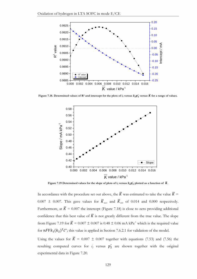
Oxidation of hydrogen in LTA SOFC in mode E/CE
129
Figure 7.18. Determined values of R2 and intercept for the plots of i2 versus 𝟐𝒑𝟐′ versus for a range of values.
Figure 7.19 Determined values for the slope of plots of i2 versus 𝟐𝒑𝟐′ plotted as a function of .
In accordance with the procedure set out above, the was estimated to take the value =
0.007 ± 0.007. This gave values for max and min of 0.014 and 0.000 respectively.
Furthermore, at = 0.007 the intercept (Figure 7.18) is close to zero providing additional
confidence that this best value of 𝐾 is not greatly different from the true value. The slope
from Figure 7.19 for = 0.007 ± 0.007 is 0.48 ± 0.06 mA kPa-1 which is the required value
for 𝑛𝐹𝑉𝑘1(𝑘2)2𝑐∗; this value is applied in Section 7.6.2.1 for validation of the model.
Using the values for = 0.007 ± 0.007 together with equations (7.53) and (7.56) the
resulting computed curves for i2 versus 𝑝2′ are shown together with the original
experimental data in Figure 7.20.
0.000 0.002 0.004 0.006 0.008 0.010 0.012 0.014 0.016
0.9885
0.9890
0.9895
0.9900
0.9905
0.9910
0.9915
0.9920
0.9925
R2 value
Intercept
value / kPa-1
R2 v
alu
e
K
-0.25
-0.20
-0.15
-0.10
-0.05
0.00
0.05
0.10
0.15
0.20
In
terc
ep
t /
mA
0.000 0.002 0.004 0.006 0.008 0.010 0.012 0.014 0.016
0.40
0.42
0.44
0.46
0.48
0.50
0.52
0.54
0.56
0.58
K value / kPa-1
Slope
Slo
pe /
mA
kP
a-1

Oxidation of hydrogen in LTA SOFC in mode E/CE
130
Figure 7.20. The ‘refined’ plot: steady anodic current versus 𝒑𝟐′ . Compare Figure 7.4.
7.6.2. Additional mechanistic theory for CE mode
A further case is now considered where the inert gas, Ar, is first bubbled through the tin
for sufficient time to reduce the hydrogen concentration to a value close to zero. Then,
while holding the potential at a constant value, E, a gas mixture of Ar/H2 with hydrogen
partial pressure p2’ is bubbled continuously, starting at time t = t1, through the tin and the
anodic current (due to injection of oxygen to replace that consumed by hydrogen) is
measured as a function of time.
At t = t1, 𝑐 = 𝑐∗ and thus i = 0 (see Equation (7.7))
Equation (7.30) becomes
[𝑑
𝑑𝑡]𝑡=𝑡1
= −𝑉𝑘1(𝑘2)2𝑐∗𝑝′
2
(7.63)
Differentiating Equation (7.35):
[𝑑𝑖
𝑑𝑡]𝑡=𝑡1
= −𝑘3𝑑𝑐
𝑑𝑡
(7.64)
From(7.43), (7.63) and (7.64):
[𝑑𝑖
𝑑𝑡]𝑡=𝑡1
= 𝑘1(𝑘2)2𝑘3𝑐
∗𝑝′2
(7.65)
Alternatively, a similar equation may be derived as follows:
Equation (7.52) becomes
ln (1 −
𝑖
𝑖2) = −
𝑘3𝑉𝑛𝐹𝑧2
(𝑡 − 𝑡1) (7.66)
0 5 10 15 20 25
0
2
4
6
8
10
data from Fig. 9
An
od
ic s
tea
dy c
urr
en
t /
mA
p'2 / kPa
maxK
minK
bestK
Oxidation of hydrogen in LTA SOFC in mode E/CE
131
as 𝑝1′ = 0 and 𝑖1 = 0 at 𝑡 = 𝑡1. For
𝑖
𝑖2≪ 1 the logarithm linearises as follows:
ln (1 −
𝑖
𝑖2) ≅ −
𝑖
𝑖2
(7.67)
So
𝑖
𝑖2≅
𝑘3𝑉𝑛𝐹𝑧2
(𝑡 − 𝑡1) (7.68)
Differentiating and combining with (7.53):
[𝑑𝑖
𝑑𝑡]𝑖𝑖2≪1≅ 𝑘1(𝑘2)
2𝑘3𝑐∗𝑝′
2
(7.69)
Thus
[𝑑𝑖
𝑑𝑡]𝑖𝑖2≪1≅ [𝑑𝑖
𝑑𝑡]𝑡=𝑡1
(7.70)
Equation (7.67) is a fair approximation for i/i2 values up to 0.2. Thus a plot of i versus t is
expected to show a straight line for values of current up to at least one fifth of the steady
current for a given hydrogen partial pressure.
Equations (7.65) and (7.70) predict that [𝑑𝑖
𝑑𝑡]𝑡=𝑡1
or [𝑑𝑖
𝑑𝑡] 𝑖𝑖2≪1
should be proportional to p2’;
a plot of [𝑑𝑖
𝑑𝑡]𝑡=𝑡1
vs. p2’is expected to reveal a slope of 𝑘1(𝑘2)
2𝑘3𝑐∗, which will be
denoted as s1.
Equation (7.53) indicates that a plot of i2 vs. 𝑧2𝑝2′ has a slope of 𝑛𝐹𝑉𝑘1(𝑘2)
2𝑐∗, which will
be denoted as s2. It follows that:
s1𝑠2=𝑘3𝑉𝑛𝐹
(7.71)
Thus the magnitude of 𝑘3
𝑉𝑛𝐹 from Equation (7.71) can be compared to the reciprocal time
constant determined from the slopes of plots of ln(i2-i) vs. t [or ln(i-i2) vs. t] at 𝑝2′=0 (see
Equation (7.52)).
7.6.2.1. Experimental validation of additional
mechanistic theory
In order to validate this extension of the theory, the cell was first flushed with a mixture of
H2/Ar to remove any residual SnO2, followed by Ar only while the tin electrode was held
at -0.90 V vs. RE at 780 °C; the ongoing parasitic leak of oxygen inevitably occurring was
measured using the technique described in Section 7.3.1. The p(H2) was then stepped from

Oxidation of hydrogen in LTA SOFC in mode E/CE
132
zero to 10 kPa and back to zero; from zero to 20 kPa and back to zero and finally from
zero to 30 kPa and back to zero. The current response was monitored with time (Figure
7.21).
Figure 7.21. Anodic current versus time in LTA SOFC at 780 °C with instantaneous step change of p(H2) from 0 to 10 kPa, then to back to zero, repeated with 20 kPa and 30 kPa.
The following current – time curves (Figure 7.22a-Figure 7.22c) were extracted from the
data in Figure 7.21. Anodic current immediately after the switch of the hydrogen from zero
to a particular partial pressure (10, 20 and 30 kPa) is shown versus time.
All three current-time curves resulted in straight lines (R2 > 0.98), the slopes (di/dt) of
which were then plotted against hydrogen partial pressure to derive the value of s1 (Figure
7.22d; Equation (7.65)). It should be noted that the straight line in Figure 7.22d is based
upon only 3 points but that each point is determined using a substantial data set;
furthermore, as predicted the intercept is small (- 0.18 × 10⁻³ mA s-1) indicating direct
proportionality between di/dt and 𝑝2′ .
5 10 15 20
0
2
4
6
8
10
H2 =
0 kP
a
H2=
10 k
Pa
100%
Ar
Time / 103 s
Cu
rrent / m
A
ianodic
at -0.90 V vs. RE
H2
=20 k
Pa
H2 =
0 k
Pa
H2
= 3
0 k
Pa
H2=
0 k
Pa

Oxidation of hydrogen in LTA SOFC in mode E/CE
133
Figure 7.22. Current-time curves after switching the hydrogen partial pressure from 0 to 10 kPa (a); 20 kPa (b); 30 kPa(c). Slopes of the lines in (a-c) vs. p(H2) are shown in (d).
The data are interpreted using Equations (7.65) and (7.70):
𝑠1 = 𝑘1(𝑘2)2𝑘3𝑐
∗ = 3.4 × 10⁻⁴ 𝑚𝐴 𝑠−1 𝑘𝑃𝑎−1
It is shown in Section 7.6.1that
𝑠2 = 𝑛𝐹𝑉𝑘1(𝑘2)2𝑐∗ = 0.48 ± 0.06 mA kPa−1
Thus applying (7.71):
s1
𝑠2=
𝑘3
𝑉𝑛𝐹=
3.4 ×10⁻⁴
0.48± 0.06 = (0.71 ± 0.09) × 10-3 s-1
This value may be compared with the value of the reciprocal time constant at 𝑝2′=0
(𝑧2 = 1) which is 0.97 × 10⁻³ s-1 (see Table 7.1).
The similarity of the determined values for the reciprocal time constant, (𝑘3
𝑉𝑛𝐹): 0.71 × 10⁻³
and 0.97 × 10⁻³ s-1, is remarkable considering that the values were determined by unrelated
methods and the simplicity of the model employed. This indicates that the principles and
assumptions upon which the model is based are broadly correct.
It is difficult to place accuracy on the assumptions employed in the CE model. However,
the correlation between the results from static (steady currents vs. p(H2)) and dynamic
measurements (step changes in p(H2) with analysis of current vs. time and di/dt
determination) is remarkable, and provides confidence in the validity of the assumptions
implied.
10 15 20 25 30
3
4
5
6
7
8
9
10
(d)
R² = 0.99
Slo
pe / 1
0-3 m
A s
-1
p(H2) / kPa
18.3 18.4 18.5 18.6 18.7-0.5
0.0
0.5
1.0
1.5
2.0
2.5
3.0
3.5
4.0
(c)
R² = 0.99
p(H2)=30 kPa
Cu
rre
nt
/ m
A
Time / 103 s
6.7 6.8 6.9 7.0
0.0
0.5
1.0
1.5
2.0
2.5
3.0
(b)
p(H2)=20 kPa
Time / 103 s
Curr
ent
/ m
A
R² = 0.99
3.55 3.60 3.65 3.70 3.75 3.80 3.85
0.0
0.2
0.4
0.6
0.8
1.0
R² = 0.99
p(H2)=10 kPa
Cu
rre
nt
/ m
A
Time / 103 s
(a)

Oxidation of hydrogen in LTA SOFC in mode E/CE
134
7.7. Conclusion
Studies of the oxidation of hydrogen in a SOFC with molten tin anode were carried out.
The anode was operated at -0.90 V versus an air RE, which is within an ‘inert’ potential
window. Steady anodic currents were essentially proportional to hydrogen partial pressure
and independent of total gas flow rate. Two models were considered for either (i) direct
anodic oxidation of dissolved hydrogen or (ii) homogeneous reaction between dissolved
hydrogen and oxygen followed by anodic injection of oxygen to replace that removed by
the chemical reaction. The former model was rejected as it required the incorporation of
the hydrogen/ argon fuel gas in the form of a persistent foam which was not detected.
Oxygen solubility values are compatible with the latter model which was validated using
steady-state and dynamic experimentally-generated data.
The development of the theoretical framework has generated the parameter 𝑧. This
parameter does not have fundamental significance but is of technological importance when
designing LMA SOFC reactors. Theory shows that 𝑧 depends upon geometric factors
(including electrode area and the volume of tin), mass-transfer (diffusion layer thickness
and diffusion coefficient of dissolved oxygen) and kinetic factors in the cell; its physical
meaning is related to the Damkohler number, widely applied in chemical reaction
engineering. The value of 𝑧 is required in order to obtain a fuller understanding of
experimentally-generated results.
This study has clarified the behaviour of the oxygen-hydrogen-tin system in the ‘inert
window’ and provides a firm basis for proceeding with studies via the Rotating Electrolyte
Disc (RED).

Additional validation of CE model
135
8. Additional validation of
CE model In the previous chapter a model for the processes taking place in the liquid metal anode
involving hydrogen oxidation in liquid tin anode SOFCs in mode CE was proposed and
validated. A new key parameter, the dynamic oxygen utilisation coefficient, (𝑧) was also
introduced which has important implications regarding understanding and design of these
systems. This chapter demonstrates the development and application of a method named
anodic injection coulometry (AIC), for the determination of 𝑧, as well as providing
additional validation of the chemical – electrochemical (CE) model by measurement of the
oxygen solubility in liquid tin for comparison with literature values.

Additional validation of CE model
136
8.1. Introduction
Solid oxide fuel cells (SOFCs) with liquid metal anodes (LMAs) have substantial potential
for power generation. The advantages over combustion systems and other types of fuel cell
have been reviewed recently130. The technology is able to provide high efficiency and low
environmental impact with flexibility regarding fuels, including solid fuel such as coal18. It is
clear that the development of pilot plants and industrial systems requires an in-depth
understanding and solutions to a number of technological challenges.
In the previous Chapter, the fundamental electrochemistry of a simple system, using
hydrogen as fuel, was explored. It was demonstrated that the oxidation of hydrogen takes
place via a chemical-electrochemical (CE) mode, whereby hydrogen undergoes
homogeneous oxidation by oxygen dissolved in the liquid tin followed by anodic oxygen
injection to replace oxygen removed by the chemical reaction. A model was developed
which was validated using experimental data. A new key parameter, termed the dynamic
oxygen utilisation coefficient, (𝑧), evolved during model development which is important
for LMA fuel cell design.
In this paper, the model is developed further and a method is proposed, named anodic
injection coulometry (AIC), similar in principle to the well-known technique of anodic
stripping voltammetry (ASV)155, to determine 𝑧. This allows the solubility of oxygen in the
melt to be measured and provides additional validation of the model and CE mechanism.
8.2. Background literature concerning oxygen
and hydrogen solubilities
Solubility of diatomic gases in liquid metals has previously been investigated by various
methods.149,156,157 It is known that dissolution of diatomic gases in liquid metals involves
dissociation into single atoms, according to Sievert’s law150,151,158,159. For example
hydrogen dissolves as follows:
𝐻2(𝑔𝑎𝑠) → 2𝐻(𝑠𝑜𝑙𝑢𝑡𝑖𝑜𝑛) (8.1)
Sievert’s law states that concentration of dissolved gas in liquid metal is proportional to the
square root of the gas partial pressure, i.e.:
𝑐′ = 𝐾𝑠√𝑝(𝐻2) (8.2)
where c’ is the concentration of dissolved hydrogen, p(H2) is the hydrogen gas pressure and
Ks is the temperature-dependent constant (Sievert’s constant).
Studies on hydrogen and oxygen solubility in liquid tin have been explored in the literature
review of this thesis (see Section 2.3.3).

Additional validation of CE model
137
Oxygen solubility in liquid tin data reported by Belford and Alcock79 and Ramanarayanan
and Rapp80 are shown in Figure 8.1.
Figure 8.1 Reported solubility of oxygen in liquid tin.
These literature values at 780 °C calculated from formulae given by Belford and Alcock79
and Ramanarayanan and Rapp80 (i.e. 0.06 and 0.08 at.%, respectively, Figure 8.1) are used
for the comparison with experimentally measured solubility data for oxygen determined in
the present chapter.
A detailed review of oxygen solubility in liquid tin (given in Section 0 of this thesis) shows a
substantial range of literature values derived from various Sn-O phase diagrams, including
both measured and predicted data. Importantly, solubility of oxygen in liquid tin is a
parameter of technological significance for operation of LMA SOFCs; this is because
operation of the liquid tin anode involves oxidation of fuel by the dissolved oxygen6.
Hence the solubility of oxygen in tin governs the quantity of oxygen which is stored
(available to react with fuel) in the liquid tin anode prior to formation/ precipitation of
solid tin oxide.
The solid oxide builds up progressively upon further polarisation of the anode and
eventually blocks the anode / electrolyte interface6,72. This phenomenon was found to be
the major cause of performance degradation of SOFCs with liquid tin anode72,73. Therefore
an in-depth understanding of oxygen solubility in liquid metal anodes is of great
importance for the development of this class of fuel cell, where oxygen solubility is a vital
parameter for design of such systems.
500 550 600 650 700 750 800
-0.01
0.00
0.01
0.02
0.03
0.04
0.05
0.06
0.07
0.08 Calculated by Ramanarayanan and Rapp
16
Measured by Belford and Alcock15
Extrapolated from Belford and Alcock15
Ns
O (
Sn
) / a
t.%
Temperature / C

Additional validation of CE model
138
This chapter presents further investigation into the role of dissolved oxygen in liquid tin
anode SOFCs when operated in CE mode. This includes determination of the key
parameter, 𝑧, as well as calculation of oxygen solubility. To this end, two related regimes of
operation are proposed. These regimes are run in a mixed mode (i.e. potentiostatic and
open-circuit), whereby electrode potential is switched between a fixed value E and open-
circuit. During the open-circuit periods hydrogen reacts with oxygen dissolved in tin. In the
first regime (Regime 1) the flow of H2 is constant, whereas in the second (Regime 2) it is
intermittent. This uses additional theory developed specifically for each regime as well as
theory developed previously160 (see Chapter 7, Section 7.6).
8.3. Experimental procedure
Experimental work employed SOFC with liquid tin anode in mode CE at 780 °C as
described previously160 (in Chapter 7).
8.4. Results and discussion
This chapter presents further validation of the theory developed to describe CE mode
hydrogen oxidation in LMA-SOFCs. Anodic injection coulometry (AIC) (with similarities
to anodic stripping voltammetry) is proposed as a method for determination of dynamic
oxygen utilisation coefficient, 𝑧, postulated in the CE model160. The method involves AIC
under two different modes of oxygen injection (termed Regimes 1 and 2). Subsequent
analysis of the experimental data in both regimes enables the calculation of 𝑧. The theory
developed previously is extended and then applied for the determination of the solubility of
oxygen in liquid tin.
8.4.1. Determination of the dynamic oxygen utilisation
coefficient using anodic injection coulometry
In the previous chapter it was shown that 𝑧 depends upon geometric factors (electrode area
and liquid metal volume), diffusion layer thickness (and hence degree of convection) and
hydrogen partial pressure. Though not fundamental, it is important to determine its value
in order to obtain an understanding of experimentally-generated results. In a broader sense,
this parameter is expected to be important for the design of systems consisting of two
processes: fuel oxidation via dissolved oxygen and oxygen replacement via electrochemical
injection at the liquid anode / electrolyte interface.
In the theoretical treatment, hydrogen and oxygen are denoted by single prime and bar
superscripts respectively, for example c’ and 𝑐 (as previously employed in Chapter 7).

Additional validation of CE model
139
8.4.1.1. Regime 1
Consider the following, four-stage operation (see Figure 8.2): prior to Point A, argon is
bubbled through liquid tin for a sufficient time to allow the current to reduce to a value
close to zero while holding the tin electrode at an anodic potential E, typically -0.90 V vs.
RE (air electrode). It has been shown that this potential places the system in the CE mode
of operation160. During the intervals A - B, B - C and C - D, hydrogen at partial pressure p’2
is bubbled through the tin. The interval A - B is sufficiently long to allow the current to
reach a steady value, i2. During the interval B - C, of length t3-t2, the tin electrode is
switched to open circuit (OC). Then, during the interval C - D, the potential of the tin
electrode is held at anodic potential E, during which time the current is monitored. The
period C - D is sufficiently long to allow the current to return to a value close to the steady
value, i2. The charge, Q1, shown as the shaded area in Figure 8.2 is then calculated.
Figure 8.2 Schematic representation of Regime 1 conditions applied to the working cell: same hydrogen partial pressure, p’
2 is applied from A to D; potential is held at a value E everywhere except in B - C.
The interval A-B was treated previously in Chapter 7 (Section 7.6.1). The interval B - C is
treated as follows. At open circuit, i=0, so the equation expressing the rate of removal of
oxygen via chemical reaction with hydrogen and the addition of oxygen via anodic injection
(Equation (7.30)) (when treated from B – C) becomes:
𝑑
𝑑𝑡= −𝑉𝑘1(𝑘2)
2𝑐 𝑝2′
(8.3)
Using Equation (7.43) shown before:
𝑑𝑐
𝑑𝑡=1
𝑉
𝑑
𝑑𝑡
We obtain:
𝑑𝑐
𝑑𝑡= −𝑘1(𝑘2)
2𝑐 𝑝2′
(8.4)
Integrating (8.4):
A B
C
D
O C

Additional validation of CE model
140
∫
𝑑𝑐
𝑐
𝑐3
𝑐2
= −𝑘1(𝑘2)2 𝑝2
′∫ 𝑑𝑡𝑡3
𝑡2
(8.5)
𝑙𝑛𝑐3𝑐2= −𝑘1(𝑘2)
2 𝑝2′(𝑡3 − 𝑡2)
Or
𝑐3 = 𝑐2exp[ −𝑘1(𝑘2)2 𝑝2
′(𝑡3 − 𝑡2)] (8.6)
The region C-D is now treated, where 𝑝′ = 𝑝2′. The steps used as follows:
i) The starting value of 𝑐, which is 𝑐3 is given by Equation (8.6).
ii) An expression is derived for 𝑐 as a function of time.
iii) Using the expression for 𝑐, and equations (7.35),(7.38) and (7.41)to reveal the
term (𝑖 − 𝑖2) as a function of time.
iv) Integrate (𝑖 − 𝑖2) from t3 to ∞ to obtain Q1.
Equation (7.51) that was derived previously provides the relationship between 𝑐 and t as
follows:
ln𝑐2 − 𝑐
𝑐2 − 𝑐1= −
𝑘3𝑉𝑛𝐹𝑧2
(𝑡 − 𝑡1)
and replacing 𝑐1 by 𝑐3 and 𝑡1 by 𝑡3 we obtain:
𝑐2 − 𝑐 = (𝑐2 − 𝑐3)exp [−
𝑘3𝑉𝑛𝐹𝑧2
(𝑡 − 𝑡3) ] (8.7)
From Equations (7.35) and (7.38) derived in the previous Chapter we can write:
𝑖 − 𝑖2 = 𝑘3(𝑐2 − 𝑐) (8.8)
Then with (8.7) we obtain:
𝑖 − 𝑖2 = 𝑘3(𝑐2 − 𝑐3)exp [−
𝑘3𝑉𝑛𝐹𝑧2
(𝑡 − 𝑡3) ] (8.9)
Substituting for 𝑐3 from (8.6) into (8.9) and using Equation (7.41) we obtain:
𝑖 − 𝑖2 = 𝑘3𝑧2𝑐∗1 − exp[−𝑘1(𝑘2)
2 𝑝2′(𝑡3 − 𝑡2)]
× exp [−𝑘3
𝑉𝑛𝐹𝑧2(𝑡 − 𝑡3) ]
(8.10)
The charge shown by the shaded area in the diagram (Figure 8.2) is given by:

Additional validation of CE model
141
𝑄1 = ∫ (𝑖 − 𝑖2)𝑑𝑡
∞
𝑡3
(8.11)
𝑄1 = −𝑉𝑛𝐹(𝑧2)2𝑐∗1 − exp[−𝑘1(𝑘2)
2 𝑝2′(𝑡3 − 𝑡2)]
× exp [−𝑘3
𝑉𝑛𝐹𝑧2(𝑡 − 𝑡3)]
𝑡3
∞
(8.12)
Or
𝑄1 = 𝑉𝑛𝐹(𝑧2)2𝑐∗1 − exp[−𝑘1(𝑘2)
2 𝑝2′(𝑡3 − 𝑡2)] (8.13)
Equation (8.13) is the required solution.
8.4.1.2. Corroborating experimental results in
Regime 1
To validate the above theory the LTA SOFC was operated in Regime 1. After Point A
(Figure 8.2) a mixture of H2 (16 kPa) and Ar was bubbled constantly through liquid tin
while holding a potential of WE at -0.90 V vs. RE. Once the anodic current had stabilised
at a steady value, the tin electrode was switched to open circuit (OC) remaining so for 1500
s before controlling the potential again at -0.90 V vs. RE. Once the anodic current had
returned to within 10 µA of its steady value, the electrode was again switched to OC and
held for 900 s. The above procedure was repeated with varying OC times (Figure 8.3).
Figure 8.3 Operation of the working cell under Regime 1 with 16 kPa p(H2) at 780 °C.
The values of Q1 were calculated applying numerical integration of the area under the
current-time curve (currents were measured at 5 s intervals) and are summarised in Table
8.1.
15 20 25 30
0
5
10
15
20
Open CircuitOpen Circuit
ianodic
at -0.90 V vs. RE
Q1(2100)
Q1(1500)
Q1(900)
Time / 103 s
Cu
rrent / m
A
Open Circuit
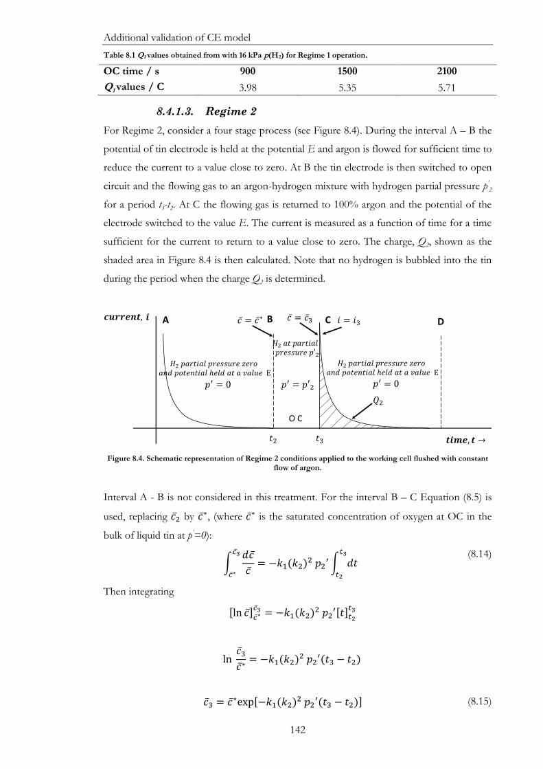
Additional validation of CE model
142
Table 8.1 Q1 values obtained from with 16 kPa p(H2) for Regime 1 operation.
OC time / s 900 1500 2100
Q1 values / C 3.98 5.35 5.71
8.4.1.3. Regime 2
For Regime 2, consider a four stage process (see Figure 8.4). During the interval A – B the
potential of tin electrode is held at the potential E and argon is flowed for sufficient time to
reduce the current to a value close to zero. At B the tin electrode is then switched to open
circuit and the flowing gas to an argon-hydrogen mixture with hydrogen partial pressure p’2
for a period t3-t2. At C the flowing gas is returned to 100% argon and the potential of the
electrode switched to the value E. The current is measured as a function of time for a time
sufficient for the current to return to a value close to zero. The charge, Q2, shown as the
shaded area in Figure 8.4 is then calculated. Note that no hydrogen is bubbled into the tin
during the period when the charge Q2 is determined.
Figure 8.4. Schematic representation of Regime 2 conditions applied to the working cell flushed with constant flow of argon.
Interval A - B is not considered in this treatment. For the interval B – C Equation (8.5) is
used, replacing 𝑐2 by 𝑐∗, (where 𝑐∗ is the saturated concentration of oxygen at OC in the
bulk of liquid tin at p’=0):
∫
𝑑𝑐
𝑐
𝑐3
𝑐∗= −𝑘1(𝑘2)
2 𝑝2′∫ 𝑑𝑡
𝑡3
𝑡2
(8.14)
Then integrating
[ln 𝑐]𝑐∗𝑐3 = −𝑘1(𝑘2)
2 𝑝2′[𝑡]𝑡2
𝑡3
ln 𝑐3𝑐∗= −𝑘1(𝑘2)
2 𝑝2′(𝑡3 − 𝑡2)
𝑐3 = 𝑐∗exp[−𝑘1(𝑘2)
2 𝑝2′(𝑡3 − 𝑡2)] (8.15)
A B C D
O C

Additional validation of CE model
143
Region C – D is now treated, where 𝑝′ = 0. It follows that the charge, Q2, shown in the
diagram (Figure 8.4) is given by
𝑄2 = (𝑐∗ − 𝑐3)𝑉𝑛𝐹 (8.16)
Substituting for 𝑐3 from (8.15) into (8.16):
𝑄2 = 𝑉𝑛𝐹𝑐∗1 − exp[−𝑘1(𝑘2)
2 𝑝2′(𝑡3 − 𝑡2)] (8.17)
This is the required solution which may be compared with Equation (8.13).
8.4.1.4. Corroborating experimental results in
Regime 2
To validate the above theory the LTA SOFC was operated in Regime 2. A mixture of H2
(16 kPa) and Ar was bubbled through the melt while the tin electrode was held at open
circuit for 1500 s. Then the tin electrode was switched from OC to -0.90 V vs. RE and the
H2 was removed from the flow (argon continued to bubble into the tin). Once the
measured anodic current (due to anodic injection of oxygen to replace oxygen consumed
by reaction with hydrogen) had reduced to zero, the electrode was switched to OC and
remained so for 900 s with flow of 16 kPa p(H2) (Figure 8.5). The above procedure was
repeated for OC intervals of 1500 and 2100 s. The flow of argon was constant throughout
the experiment including the open circuit periods.
Figure 8.5 Operation of the working cell under Regime 2 with 16 kPa p(H2) at 780 °C.
15 20 25
0
2
4
6
8
10
Open CircuitOpen CircuitOpen Circuit
Q2(2100)
Q2(900)
Q2(1500)
ianodic
at -0.90 V vs. RE
Cu
rrent / m
A
Time / 103 s

Additional validation of CE model
144
The values of Q2 were calculated in the same way as Q1 values via numerical integration of
the area under the current-time curve (currents again were measured at 5 s intervals) and
are summarised in Table 8.2.
Table 8.2. Q2 values obtained with 16 kPa p(H2) for Regime 2 operation.
OC time / s 900 1500 2100 Q2 values / C 5.11 8.05 8.9
8.4.1.5. Regime 3
This case is included for completeness. However no experiments were performed to
support the theory developed for Regime 3 as this is not required for determination of 𝑧.
This regime, which is a combination of the previous two regimes, is illustrated in Figure
8.6.
Figure 8.6 Schematic representation of Regime 3 conditions applied to the working cell flushed with constant flow of argon; potential is held at a value E everywhere except in B - C.
Prior to Point A argon is bubbled through tin and the electrode is held at an anodic
potential E, typically -0.90 V with respect to an air electrode, while sufficient time is
allowed for the current to reduce to a value close to zero. During the intervals A – B and B
- C, hydrogen at partial pressure p’2 is bubbled through the tin. The interval A - B (with
potential maintained at E) is sufficiently long to allow the current to reach a steady value, i2.
During the interval B - C, of length t3-t2, the tin electrode is switched to open circuit. At
Point C the flowing gas is returned to 100% argon and the tin electrode switched from OC
to the potential E. Thereafter, the current is measured as a function of time until the
current returns to a value close to zero. The charge Q3 shown as the shaded area in Figure
8.6 is then calculated. Note that no hydrogen is bubbled into the tin during the period
when the charge Q3 is determined.
Following Regime 1, the oxygen concentration 𝑐3 at C given by (8.6) which together with
Equation (7.41) leads to:
A B
C D
O C

Additional validation of CE model
145
𝑐3 = 𝑧2𝑐∗exp[ −𝑘1(𝑘2)
2 𝑝2′(𝑡3 − 𝑡2)] (8.18)
For the interval C – D as for Regime 2 the partial pressure of hydrogen equals to zero
(i.e.𝑝′ = 0). It follows that the charge, Q3, shown in the diagram (Figure 8.6) is given by
𝑄3 = (𝑐∗ − 𝑐3)𝑉𝑛𝐹 (8.19)
So from (8.18) and (8.19):
𝑄3 = 𝑉𝑛𝐹𝑐∗1 − 𝑧2exp[−𝑘1(𝑘2)
2 𝑝2′(𝑡3 − 𝑡2)] (8.20)
This is the required solution and may be compared with (8.13) and (8.17)
Summary of the principal results in 8.4.1.1- 8.4.1.5.
The important equations in the above sections are those that allow interpretation of the
coulombic charge under the final parts of the regimes, i.e. C – D. These are as follows:
Regime 1 𝑄1 = 𝑉𝑛𝐹(𝑧2)2𝑐∗1 − exp[−𝑘1(𝑘2)
2 𝑝2′(𝑡3 − 𝑡2)] (8.13)
Regime 2 𝑄2 = 𝑉𝑛𝐹𝑐∗1 − exp[−𝑘1(𝑘2)
2 𝑝2′(𝑡3 − 𝑡2)] (8.17)
Regime 3 𝑄3 = 𝑉𝑛𝐹𝑐∗1 − 𝑧2exp[−𝑘1(𝑘2)
2 𝑝2′(𝑡3 − 𝑡2)] (8.20)
8.4.1.6. Experimental determination of dynamic oxygen
utilisation coefficient,
The development of the theoretical framework described earlier in Section 7.6, Chapter 7
has identified the parameter 𝑧. For a given hydrogen partial pressure, 𝑝2′, and (𝑡3 − 𝑡2), 𝑧
may be determined using (8.13)and (8.17)as follows:
(𝑧2)
2 =𝑄1𝑄2
(8.21)
Taking the values of Q1 and Q2 from Table 8.1 and Table 8.2, the value of 𝑧2 from (8.21) is
equal to 0.83 for hydrogen partial pressure of 16 kPa.
The estimated uncertainty on the obtained values of Q1 and Q2 is ± 5%, resulting in an
uncertainty in the 𝑧2 value of 3.5 % (i.e. 𝑧2 =0.83 ± 0.03).
The relationship between a value of 𝑧2 and 𝑝2′was shown in Equation (7.56) as follows:
𝑧2 = (1 + 𝑝2′ )−1 (7.56)
Taking 𝑧2 as 0.83 for 16 kPa p(H2) and inserting into (7.56) leads to a value of of 0.012
kPa-1. This value within the range of values of (0.000< <0.014 kPa-1) deduced in
Chapter 7.

Additional validation of CE model
146
8.4.2. Measurement of the oxygen solubility in liquid tin
using electrochemical model for CE mode
Having obtained a value for 𝑧2, the solubility of oxygen in tin (oxygen content at an
electrode potential of -0.90 V versus air electrode) may be determined as shown below. The
value calculated may then be compared with literature values and used to provide
additional validation and confirmation of the model developed and tested in Chapter 7.
An expression for the number of moles of dissolved oxygen in liquid tin, may be developed
using the Equations (7.38)and (7.41) as follows:
𝑖2 = 𝑘3(𝑐∗ − 𝑐2) (7.38)
𝑐2 = 𝑧2𝑐∗ (7.41)
Eliminating 𝑐2 between (7.38)and (7.41) leads to:
𝑖2 = 𝑘3𝑐∗(1 − 𝑧2) (8.22)
We can write this as
𝑖2 =
𝑘3𝑐∗𝑉𝑛𝐹 (1 − 𝑧2)
𝑉𝑛𝐹
(8.23)
Rearranging (8.23):
𝑐∗ =
𝑖2(1 − 𝑧2)𝑛𝐹𝑉
(𝑉𝑛𝐹
𝑘3)
(8.24)
This is an expression for the saturated concentration of oxygen in liquid tin, 𝑐∗, in terms of
the steady current, i2, the time constant at p’=0 (when 𝑧2=1), 𝑉𝑛𝐹
𝑘3, the volume of tin, V, and
the parameter 𝑧2.
Recalling Equation relating the steady anodic current and p(H2) that was presented in
Figure 7.4 (current in mA hydrogen partial pressure in kPa):
isteady=0.42p(H2)+0.15 (8.25)
the value of i2 for 16 kPa can be determined from that.
Similarly the time constant, 𝑉𝑛𝐹
𝑘3, for p(H2)=0 was reported as 1031 s (refer to Table 7.1).
Substituting the value of 𝑧2 =0.83 determined in the previous section for 16 kPa p(H2), the
solubility of oxygen, 𝑐∗ is found to be 5.7 × 10⁻⁵ mol cm-3 or 0.10 at.% .
The potential of the working electrode was chosen to be close (within 10 mV) to the
equilibrium potential of the Sn/SnO2 couple. At this potential the oxygen concentration is
expected to be close to the saturated value. Moving to more positive potentials would
result in precipitation of SnO2 (see Figure 6.3).

Additional validation of CE model
147
The calculated value (0.10 at.% at 780 °C) is comparable to those reported by
Ramanarayanan and Rapp80 (0.08 at.%) and Belford and Alcock79 (0.06 at.%), respectively.
This serves as additional confirmation for the validity of the electrochemical model
developed for CE mechanism in the previous Chapter.
8.5. Conclusion
Operation of LMA SOFC fuelled with hydrogen in mode CE was investigated using the
newly-developed anodic injection coulometry technique applied in two regimes of
operation. Analysis of experimentally-generated data (Q1 and Q2 values measured in
Regimes 1 and 2, respectively) resulted in the value of dynamic oxygen utilisation
coefficient, 𝑧, determined for 16 kPa hydrogen as 0.83. The oxygen solubility in liquid tin at
780 °C was measured to be 0.10 at.%, which is similar to literature values, serving as
additional confirmation of the validity of the model for CE mode operation.

Water electrolysis in reverse LME SOFCs
148
9. Water electrolysis in
reverse LME SOFCs This chapter examines reduction of water (steam) in reverse liquid tin anode SOFCs (or
solid oxide electrolysers – SOEs). Possible mechanisms for the electrolysis of water in
LMA are proposed. The most likely mechanism is considered to be dissolution of water
(fast process), followed by slow, rate-determining, dissociation of water to hydrogen and
oxygen and then by diffusion-controlled cathodic extraction of the oxygen generated by the
dissociation of water. Hydrogen generated by the electrolysis was carried out of the cell
with the carrier gas. Saturation of the carrier gas with water vapour was achieved using
water bottles held at either at room temperature or at temperatures below ambient using a
water bath (cooled with ice) with thermostat. Partial pressure of water vapour was varied
to investigate its effect on measured current. Initial results showed that, upon changing the
water vapour content of the carrier gas, measured current- time curves followed an
exponential function, with time constants somewhat shorter than those measured for
hydrogen oxidation (followed by anodic injection of oxygen). Currents eventually stabilised;
steady currents were found to be proportional to partial pressure of water vapour. An
electrochemical model has been developed for interpretation of the water reduction data.
The model was validated with experimental results and overall good agreement was found.
Initial studies only are presented here and additional work is required for a more complete
understanding of water electrolysis in reverse LMA SOFCs.

Water electrolysis in reverse LME SOFCs
149
9.1. Introduction
There are numerous studies on water electrolysis for production of hydrogen using solid
oxide membranes161. The use of solid oxide electrolysers (SOE) is advantageous due to
availability and application of heat that is emitted (wasted) during various industrial
processes. However, high energy requirement for water (steam) dissociation remains to be
the greatest challenge162,163. Many studies have suggested the use of gaseous hydrocarbons
to reduce the open circuit voltage in solid oxide steam electrolysers (SOSE)162,163. One of
the most relevant studies was made by Pati et al. where instead of solid anode with gaseous
carbonaceous fuel, the SOSE was operated on solid hydrocarbon fuel53,56 fed into a liquid
metal anode to provide an interface for solid fuel oxidation.
Water electrolysis for production of syngas (a mixture of H2 and CO) from steam and
hydrocarbon waste in such cells was achieved using a solid oxide electrolyte, Ni-YSZ
cathode and liquid tin anode53,56. Oxidation of fuel in liquid metal anode reduces the
concentration of dissolved oxygen in the metal anode and aids the dissociation of steam to
hydrogen53.
The steam is fed to the cathode (Ni-YSZ) and undergoes the reaction as follows:
𝐻2𝑂(𝑔) + 2𝑒−(𝑁𝑖) → 𝐻2(𝑔) + 𝑂
2− (9.1)
Oxygen ions are then oxidised at the interface with the melt as follows:
𝑂2− → [𝑂]𝑆𝑛 + 2𝑒− (9.2)
Dissolved oxygen diffuses through the liquid metal to react with the reductant (fuel) via
reaction as follows:
[𝑂]𝑆𝑛 + 𝑅 → 𝑅𝑂(𝑔) (9.3)
The schematic of the operation of a solid oxide electrolyser with LMA was described
earlier in the literature review (Chapter 2; Figure 2.16). The electrolysis of steam using the
liquid metal electrode has not previously been reported.
This chapter aims to investigate the possibility for water (steam) electrolysis within the
liquid metal electrode. The approach applied in the present study whereby water (steam)
dissociates in a liquid metal electrode has not been tested previously in typical solid oxide
electrolysers (SOE) and hence provides some new insights into the application of liquid
metal electrodes for water electrolysis.
9.2. Experimental procedure
In the present chapter, all experimental work entails operation of LTA SOFC cell at a
constant operating temperature of 810 °C. Experimental set-up and components of the
working cell were similar to the ones described in Chapter 4. However, some modifications
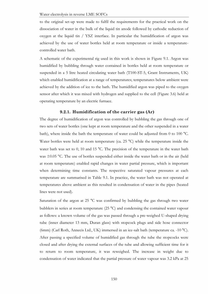
Water electrolysis in reverse LME SOFCs
150
to the original set-up were made to fulfil the requirements for the practical work on the
dissociation of water in the bulk of the liquid tin anode followed by cathodic reduction of
oxygen at the liquid tin / YSZ interface. In particular the humidification of argon was
achieved by the use of water bottles held at room temperature or inside a temperature-
controlled water bath.
A schematic of the experimental rig used in this work is shown in Figure 9.1. Argon was
humidified by bubbling through water contained in bottles held at room temperature or
suspended in a 5 litre heated circulating water bath (T100-ST-5, Grant Instruments, UK)
which enabled humidification at a range of temperatures; temperatures below ambient were
achieved by the addition of ice to the bath. The humidified argon was piped to the oxygen
sensor after which it was mixed with hydrogen and supplied to the cell (Figure 3.6) held at
operating temperature by an electric furnace.
9.2.1. Humidification of the carrier gas (Ar)
The degree of humidification of argon was controlled by bubbling the gas through one of
two sets of water bottles (one kept at room temperature and the other suspended in a water
bath), where inside the bath the temperature of water could be adjusted from 0 to 100 °C.
Water bottles were held at room temperature (ca. 25 °C) while the temperature inside the
water bath was set to 0, 10 and 15 °C. The precision of the temperature in the water bath
was ±0.05 °C. The use of bottles suspended either inside the water bath or in the air (held
at room temperature) enabled rapid changes in water partial pressure, which is important
when determining time constants. The respective saturated vapour pressures at each
temperature are summarised in Table 9.1. In practice, the water bath was not operated at
temperatures above ambient as this resulted in condensation of water in the pipes (heated
lines were not used).
Saturation of the argon at 25 °C was confirmed by bubbling the gas through two water
bubblers in series at room temperature (25 °C) and condensing the contained water vapour
as follows: a known volume of the gas was passed through a pre-weighed U-shaped drying
tube (inner diameter 13 mm, Duran glass) with stopcock plugs and side hose connector
(6mm) (Carl Roth, Annecis Ltd., UK) immersed in an ice-salt bath (temperature ca. -10 °C).
After passing a specified volume of humidified gas through the tube the stopcocks were
closed and after drying the external surfaces of the tube and allowing sufficient time for it
to return to room temperature, it was reweighed. The increase in weight due to
condensation of water indicated that the partial pressure of water vapour was 3.2 kPa at 25

Water electrolysis in reverse LME SOFCs
151
°C (in agreement with the value given by standard tables) showing that the gas was fully
saturated with H2O.
Table 9.1 Saturated water vapour pressure at set temperature values from standard tables.
Temperature / °C 0 10 15 25 26 28
p(H2O) / kPa 0.6 1.2 1.7 3.2 3.4 3.8
Figure 9.1 Process flow diagram for dissociation of water in LMA SOFC cell followed by cathodic reduction of oxygen (with optional use of H2 for additional removal of tin oxide).
9.3. Results and discussion
9.3.1. Water reduction in LTA SOFC
The water bath was operated at temperatures of 0, 10, and 15 °C (below the room
temperature of 26 °C) which eliminated condensation inside the tubing. The LTA SOFC
cell was run at 810 °C and dry argon at a flow rate of 1ml s-1 was supplied to the cell. A
potential of -1.1 V vs. RE was applied to the working electrode (WE).
The flow of argon was switched between water bottles held at room temperature (26 °C)
and others suspended in the water bath at temperatures below ambient. The temperature of
each set of water bottles was maintained constant throughout each experiment.
H2
Ar
Water Bottles
Oxygen
Sensor
Water Bottles
To
extraction
F
Ball valve Filter
F
Mass Flow Controller Three Way Valve
KEY
Thermocouple
Working electrode
(WE)
Reference
electrode (RE)
Counter electrode (CE)
H2/Ar(H2O) in
H2/Ar (H2O), O2 out
dry Ar
Water Bath
humidified Ar
F

Water electrolysis in reverse LME SOFCs
152
The observed cathodic current with time is shown in Figure 9.2. Initially it gradually
decreased in magnitude from ca. -10 mA and stabilised at ca.-1.0 mA with dry argon
(Figure 9.2).
The flow of argon was then switched to bubble through bottles in the water bath which
was set to 0 °C. This resulted in a steady current of -1.8 mA. The flow of argon was then
changed so that it was supplied through two water bottles (held at room temperature) and
the cathodic current increased in magnitude to -4.6 mA associated with 3.4 kPa p(H2O).
The procedure was repeated whereby the carrier gas was supplied from bottles at 0, 10 and
15 °C. The estimated accuracy of measured currents is ± 50 µA.
Figure 9.2 Cathodic current at -1.1 V vs. RE at 810 °C with changes of p(H2O).
The steady currents as a function of p(H2O) (corrected for the reduction current attributed
to parasitic oxygen concentration in the melt) are shown in Figure 9.3. Linearity between
the steady cathodic current and p(H2O) is evident (R2>0.98). The uncertainty on the points
in this Figure is estimated ±75 µA in the current and ±0.2 kPa in p(H2O).
Figure 9.3 Steady cathodic current data as a function of p(H2O) corrected for parasitic oxygen current.
0 5 10 15 20 25 30
-10
-8
-6
-4
-2
0
15 C 10 C
28 C
10 C
dry Ar
0 C
28 C
0 C
dry Ar
Curr
ent
/ m
A
Time / 103 s
-0.5 0.0 0.5 1.0 1.5 2.0 2.5 3.0 3.5
-4.0
-3.5
-3.0
-2.5
-2.0
-1.5
-1.0
-0.5
0.0
0.5
isteady
= -1.07p(H2O)-0.13
R2=0.983
icathodic
, mA
Equation
Weight
Residual Sum of Squares
Pearson's r
Adj. R-Square
C2
Ste
ady c
ath
odic
curr
ent /
mA
p(H2O) / kPa

Water electrolysis in reverse LME SOFCs
153
Interestingly, measured steady cathodic currents during water reduction (at -1.1 V) were
greater in magnitude (by a factor of 2.5) than steady anodic currents for hydrogen oxidation
(at -0.90 V) for a given partial pressure of either hydrogen or water vapour.
9.3.2. Water reduction in Regime 1
Operating conditions of Regime 1 (refer to Chapter 8) were applied for water reduction at
810 °C. Instead of anodic overvoltage, a potential of -1.1 V vs. RE was applied to the tin
electrode with open circuit (OC) intervals of 300, 1500, 900 and 2100 seconds (Figure 9.4).
The water vapour pressure was maintained constant at a value of 3.8 kPa corresponding to
28 °C with a flow of Ar 1 ml s-1. The estimated accuracy of current measurements is ±
10µA.
Figure 9.4 Operation of LTA SOFC under Regime 1 with constant 3.8 kPa p(H2O).
Q1 values (coulombic charge to reduce dissolved oxygen generated during the open-circuit
periods due to the water dissociation process in liquid tin) were calculated by numerical
integration of the area under the current vs. time curve (Figure 9.4) and are summarised in
Table 9.2. The estimated uncertainty on the obtained values of Q1 is ± 2.5%.
Table 9.2 Q1 values obtained from with 3.8 kPa p(H2O) for Regime 1 operation.
OC time / s 300 900 1500 2100
Q1 values / C 1.3 3.6 5.2 7.1
The obtained values of Q1 increase in magnitude as the open-circuit period rises indicating
that dissolved oxygen concentration increases with time. A plot of measured Q1 values (in
mC) versus the open circuit intervals resulted in a straight line with a slope of -4.3 mC s-1
(Figure 9.5). This slope divided by the vapour pressure of water vapour leads to the value -
2 4 6 8 10 12 14 16 18 20
-40
-30
-20
-10
0
Cu
rre
nt
/ m
A
Time / 103 s
i cathodic
at -1.1 V vs. RE
Open Circuit Open Circuit Open Circuit Open Circuit
Q1(300)
Q1(1500) Q
1(900)Q
1(2100)
Water electrolysis in reverse LME SOFCs
154
1.1 mA kPa-1 in agreement with the slope of Figure 9.3. This important finding is relevant
to the development of an electrochemical model for interpretation of experimentally-
generated results. The estimated accuracy of Q1 values is ± 100 mC.
Figure 9.5 Measured Q1 values as a function of OC intervals.
9.3.3. Electrochemical model for water electrolysis
The CE model was developed for the oxidation of hydrogen to water in Chapter 7.
Measurements have been made for the reverse process, reduction of water to hydrogen.
Results showed steady current proportional to partial pressure of water vapour. Also step
changes in partial pressure of water vapour resulted in exponential-type current-time
curves. Thirdly, Q1 values increased with open-circuit period and showed values consistent
with steady currents.
A simple theory is developed below for initial interpretation of the results. Two possible
mechanisms were considered analogous to those proposed for hydrogen oxidation earlier:
i) Rate-determining dissolution of water followed by diffusion-controlled cathodic
reduction at the zirconia-tin interface.
ii) Fast dissolution of water in the tin with concentration proportional to partial
pressure of water vapour, i.e. Henry’s law behaviour (Sievert’s law only applicable
to diatomic gases), followed by rate-determining homogeneous reduction of water
and then diffusion-controlled cathodic reduction of oxygen at the zirconia-tin
interface .
Either of these mechanisms would result in a steady current proportional to the partial
pressure of water vapour but Mechanism (ii) is thought to be more likely particularly as it is
the one analogous to that validated for hydrogen oxidation and this is the one developed
below.
The reaction equation is:
0 500 1000 1500 2000 2500-10000
-8000
-6000
-4000
-2000
0
Q1=-4.3(t
3-t
2)-240
R2=0.99
Q1 values / mC
Equation
Weight
Residual Sum of Squares
Pearson's r
Adj. R-Square
C2
Q1 / m
C
OC time / s

Water electrolysis in reverse LME SOFCs
155
[𝐻2𝑂]𝑆𝑛 → 2[𝐻]𝑆𝑛 + [𝑂]𝑆𝑛 (9.4)
This injects oxygen into the tin. [𝐻]𝑆𝑛 is removed by the following associative process with
the hydrogen gas being carried out of the system by the flowing Ar carrier gas:
2[𝐻]𝑆𝑛 → (𝐻2)𝑔 ↑ (9.5)
If the Sn electrode is held at a potential, E, typically -1.1 V vs. air electrode, then the
oxygen generated via Reaction (9.4) is removed by cathodic reduction at the Sn-YSZ
interface:
[𝑂]𝑆𝑛 + 2𝑒− ⥂ 𝑂2− (9.6)
This is a similar process to that occurring as a result of H2 oxidation, except the diffusion
of oxygen and the current are in the reverse direction (refer to Equation (7.28) and Figure
7.13).
In the theoretical treatment, water concentration is denoted by double prime and oxygen
concentration by a bar.
Concentration profiles in the tin at the interface may be represented by the following
figure.
Figure 9.6 Schematic of the dissolved oxygen concentration profile at a given applied potential E during the water reduction process. The diffusion layer thickness is shown as δ. (Compare with Figure 7.13).
The rate of generation of oxygen via Reaction (9.4) is 𝑉𝑘4𝑐′′ (i.e. 𝑘4𝑐
′′ per unit volume of
tin) where k4 is the homogeneous rate constant for the reaction.
The rate of injection of oxygen via Reaction (9.6) is 𝑖 𝑛𝐹⁄ (n=2, note that i is negative).
Thus the net rate of injection of oxygen via the two reactions is 𝑉𝑘4𝑐′′ + 𝑖 𝑛𝐹⁄ . The
concentration of water, c’’, for a given water partial pressure, p’’, is given by (Henry’s law):
𝑐′′ = 𝑘5𝑝′′ (9.7)
,

Water electrolysis in reverse LME SOFCs
156
where k5 is a constant for a given temperature.
Expressing the total amount (gram atoms) of [O] in the tin as , it follows that
𝑑
𝑑𝑡= 𝑉𝑘4𝑘5𝑝
′′ +𝑖
𝑛𝐹
(9.8)
Applying Fick’s first law to the diffusion of [O] to the interface (𝐽 negative) (Figure 9.6):
𝐽 = −𝐴
𝑑𝑐
𝑑𝑥
(9.9)
, 𝐴 and 𝑑𝑐
𝑑𝑥 have their usual significance.
So (9.9) becomes:
𝐽 = −𝐴 (
𝑐 − 𝑐∗∗
𝛿)
(9.10)
Concentration 𝑐∗∗ is defined as the equilibrium concentration of [O] at potential E, the
potential at which the tin electrode is held (typically -1.1 V vs. air electrode in this case).
Equating the current with the flux via Faraday’s law:
𝐽 =
𝑖
𝑛𝐹
(9.11)
Eliminating 𝐽 between (9.10) and (9.11):
𝑖 =
𝑛𝐹𝐴
𝛿(𝑐∗∗ − 𝑐)
(9.12)
Or
𝑖 = 𝑘3(𝑐∗∗ − 𝑐) (9.13)
where 𝑘3 is given by
𝑘3 =
𝑛𝐹𝐴
𝛿
(9.14)
In the steady-state situation, when 𝑝′′ = 𝑝2′′, 𝑐 = 𝑐2, 𝑖 = 𝑖2 and
𝑑
𝑑𝑡= 0, then using (9.8)
𝑖2 = −𝑉𝑛𝐹𝑘4𝑘5𝑝2′′ (9.15)
This shows that steady current is directly proportional to the partial pressure of water
vapour (as found experimentally and with negative slope, Figure 9.3).
The model is now developed to obtain an expression for the transient behaviour (changing
from 𝑝1′′to 𝑝2
′′). The mathematics is simplified by defining a new variable, 𝑐, where
𝑐 = 𝑐∗∗ − 𝑐 (9.16)
So Equation (9.13) becomes
𝑖 = 𝑘3𝑐 (9.17)
When 𝑝′′ = 𝑝2′′, 𝑖 = 𝑖2 and Equation (9.17) becomes:
𝑖2 = 𝑘3𝑐2 (9.18)

Water electrolysis in reverse LME SOFCs
157
Eliminating i2 between (9.15) and (9.18):
𝑐2 = −
−𝑉𝑛𝐹𝑘4𝑘5𝑝2′′
𝑘3
(9.19)
And similarly:
𝑐1 = −
−𝑉𝑛𝐹𝑘4𝑘5𝑝1′′
𝑘3
(9.20)
Note that 𝑑𝑐
𝑑𝑥= −
𝑑𝑐
𝑑𝑥; 𝑑𝑐
𝑑𝑡= −
𝑑𝑐
𝑑𝑡.
Recalling that
𝑑𝑐
𝑑𝑡 =1
𝑉
𝑑
𝑑𝑡
(9.21)
So
𝑑𝑐
𝑑𝑡 = −
1
𝑉
𝑑
𝑑𝑡
(9.22)
Using Equation (9.8) with 𝑝′′ = 𝑝2′′, with (9.19), (9.17) and (9.22):
−𝑉
𝑑𝑐
𝑑𝑡 = −
𝑘3𝑐2𝑛𝐹
+𝑘3𝑐
𝑛𝐹
𝑑𝑐
𝑑𝑡 =
𝑘3𝑉𝑛𝐹
(𝑐2 − 𝑐) (9.23)
Separating the variables and integrating:
−∫
𝑑𝑐
𝑐 − 𝑐2
𝑐
𝑐1
=𝑘3𝑉𝑛𝐹
∫ 𝑑𝑡𝑡
𝑡1
ln[𝑐 − 𝑐2]𝑐1
𝑐 =𝑘3𝑉𝑛𝐹
(𝑡 − 𝑡1)
ln𝑐 − 𝑐2𝑐1 − 𝑐2
=𝑘3𝑉𝑛𝐹
(𝑡 − 𝑡1) (9.24)
Using (9.17)
ln𝑖 − 𝑖2𝑖1 − 𝑖2
=𝑘3𝑉𝑛𝐹
(𝑡 − 𝑡1) (9.25)
This is the required equation.
9.3.4. Experimental validation of the model on water
reduction in LMA SOFC
The electrochemical mode developed for water reduction in LMA SOFC was validated
against the experimental data.

Water electrolysis in reverse LME SOFCs
158
Application of Equation (9.25) derived for reduction of water on the experimental data for
water dissociation and cathodic reduction of oxygen at -1.1 V vs. RE at 810 °C (the reverse
process of hydrogen oxidation) (shown in Figure 9.2) resulted in reasonable straight lines
(R2 average > 0.94) (Figure 9.7-Figure 9.8). Note that the R-squared value is a measure of the
goodness of fit of the data to a straight line. The standard error of the slope is 5 × 10⁻⁵ s-1.
The analysis was applied only to the smoothest parts of the current-time curve, as the
remainder of the current-time curve was excessively noisy. The slopes obtained in Figure
9.7- Figure 9.8 are summarised in Table 9.3.
Figure 9.7 Step change in p(H2O): from 3.78(28 °C) to 0.61(0 °C) kPa (a); from 0.61kPa (0 °C) to zero (dry Ar) (b).
Figure 9.8 Step change in p(H2O): from zero (dry Ar) to 1.23 kPa (10 °C) (a); from 3.78 kPa (28 °C) to 1.23 kPa
(10 °C) (b).
Table 9.3. Reciprocal time constants for various destination p(H2O) values.
p(H2O)/ kPa 0 0.6 1.2
Slope / 10-3 s-1 3.04 2.57 2.74 1.70 Average slope / 10-3 s-1 1.99 Time constant / s 329 389 503
200 400 600 800-1.0
-0.5
0.0
0.5
1.0
R² = 0.977
linear fit
(t - t1) / s
ln (
i 2-i )
/ i in m
A
(a)
200 400 600 800
-3.5
-3.0
-2.5
-2.0
-1.5
-1.0
-0.5
0.0
ln (
i 2-i )
/ i in
mA
(b)
linear fit
R² = 0.895
(t - t1) / s
0 100 200 300 400 500 600
-1.4
-1.2
-1.0
-0.8
-0.6
-0.4
-0.2
0.0
0.2
0.4
0.6
(a)
R² = 0.939
linear fit
Equation
Weight
Residual Sum of Squares
Pearson's r
Adj. R-Square
D2
ln (
i -
i 2)
/ i in
mA
(t - t1) / s
200 400 600 800 1000 1200
-1.0
-0.5
0.0
0.5
1.0
ln (
i 2-i )
/ i in m
A
(b)
linear fit
(t - t1) / s
R² = 0.948
Water electrolysis in reverse LME SOFCs
159
The theory developed for H2O reduction is similar to the one for H2 oxidation where
reciprocal time constant was shown as 𝑘3
𝑉𝑛𝐹2 vs.
𝑘3
𝑉𝑛𝐹 (see Equation (9.25)). So the same
time constant (𝑧2=1) should be found for hydrogen oxidation and water reduction.
However, for the limited and noisy data available, the time constant for water reduction
was found to be significantly lower than that for hydrogen oxidation (compare data in
Table 7.1 and Table 9.3). The experiment was also more difficult to perform with water
because a step change in partial pressure of water vapour was not straightforward.
In the present study, liquid metal cathode was applied for electrolysis of water and on the
anode side (Pt solid electrode) molecular oxygen was generated. This process can be
combined with the approach proposed by Pati et al.53 and hence both cathode and anode
will be liquid metals. In that case the energy requirements for water electrolysis should
reduce, while the liquid metal anode can operate with various carbonaceous fuels (even
contaminated) and generate CO. Then the overall reaction for such system would be:
𝐻2𝑂 + 𝑅 → 𝐻2 + 𝑅𝑂 (9.26)
where R – is the carbonaceous fuel (reductant),
If for instance solid carbon is utilised on the anode side, then the system generates H2 and
CO. In line with stability and deterioration concerns of solid anodes (e.g. Ni-YSZ) with
hydrocarbons, the suggested system provides an interesting alternative to common solid
oxides steam electrolysers. However, more research is required to understand the
performance of liquid metal electrodes for both anodic and cathodic reactions.
9.4. Conclusion
Studies of the electrolysis of water in a reverse SOFC with liquid tin anode were carried
out. The tin electrode was operated at -1.1 V versus air electrode. Water vapour pressure,
p(H2O), has been varied using the water bottles and water bath where the temperature of
water had been adjusted. It was shown that it is preferable to set the temperature of the
water bath to a value below room temperature, where the lines are unheated. This resulted
in reasonably smooth current – time curves. Steady cathodic currents were proportional to
water vapour pressure, p(H2O) for the limited range investigated.
An electrochemical model for water reduction (the reverse of that shown to be applicable
to hydrogen oxidation) was developed as a theoretical framework for interpretation of
experimental data. Rapid dissolution of water in the liquid tin anode followed by rate-
determining dissociation to hydrogen and oxygen followed by diffusion-controlled cathodic
reduction of oxygen has been demonstrated as the likely mechanism for water reduction in
a reverse LMA SOFC.

Water electrolysis in reverse LME SOFCs
160
Application of the model resulted in shorter time constants for cathodic reduction of
oxygen at the liquid tin / YSZ interface compared with ones for oxygen injection during
hydrogen oxidation reported in Chapter 7.
Water reduction in Regime 1 resulted in Q1 values (the total charge for reduction of
dissolved oxygen due to its accumulation in tin from water reduction) that increased
directly proportionally with OC periods, which was expected. There was an important and
significant correlation between the rate of oxygen accumulation in the tin on open-circuit
due to dissociation of water vapour and the steady current measured on closed-circuit at
equilibrium.

Rotating Electrolyte Disc system design and testing
161
10. Rotating Electrolyte
Disc system design and
testing Experimental and modelling work presented in the previous Chapters 7-9 has clarified the
behaviour of the oxygen-hydrogen/water-tin system in the ‘inert window’ and provided a
firm basis for proceeding with studies via the Rotating Electrolyte Disc (RED) technique
being developed specifically to examine the mass-transport and kinetics processes within
the liquid metal electrode.
This chapter includes the rationale for a novel rotating electrolyte disc (RED) technique, an
inverted system based on standard rotating disc electrode (RDE) theory, to study various
transport and kinetic processes within liquid metal electrodes in the LMA SOFC. The
chapter provides details of the evolution of developed RED designs. Experimental
validation of the engineering aspects of the RED apparatus was made in an aqueous
system. The results obtained confirmed that the first prototype RED apparatus was built
correctly and performance similar to conventional commercial RDE set-ups was achieved.
Testing of the RED in molten tin anode is anticipated. Model systems that were explored
in Chapters 7-9 are now proposed to be tested with the RED.

Rotating Electrolyte Disc system design and testing
162
10.1. Introduction
With respect to uncertainties in performance of liquid metal anode SOFCs reported earlier
(Section 2.3.5), greater understanding of electrochemical reactions, redox, and transport
processes within liquid metal electrodes is needed. There are a number of research
challenges, including: mass transport of dissolved oxygen (and other gases) or oxidized
species in the liquid metal; reaction kinetics between metal oxide and fuel within the liquid
anode; kinetics of oxygen transfer at the liquid metal anode - electrolyte interface, etc.
The mechanism and kinetic characteristics of solid electrode reactions with solution phase
electroactive species is typically derived via application of the well-established rotating disc
electrode (RDE) technique99,164,165. The robust theory of the RDE has been extensively
utilised for aqueous electrochemical systems108. However, its application to examine the
mechanisms of operation of SOFCs with LME has not been previously reported.
A novel technique that is based on standard RDE theory has been developed in this study
to address research questions on transport and kinetics of electrochemical reactions within
the liquid metal electrode. In the proposed design, a solid electrolyte disc rotates in a liquid
metal electrode (e.g. tin), as opposed to a solid electrode disc rotating in a liquid electrolyte.
This underlying operating principle makes the proposed concept novel and unique. To
reflect that feature the technique is termed “Rotating Electrolyte Disc”.
The RED is designed to determine parameters controlling mass transport of dissolved
oxygen (and other gases) and oxidised species, including metal oxide in the liquid metal; the
technique also provides the possibility of the investigation of heterogeneous and
homogeneous reaction kinetics as well as the influence of electrode contaminants.
Investigation of anodic reaction kinetics can provide additional options to optimize
conventional tubular design of LME SOFCs and in turn contribute to further
improvement of fuel cell performance. The application of the RED in LMA SOFCs
involves operation with molten metal above 700 °C, as opposed to aqueous electrolyte at
ambient temperature, which is interesting and challenging at the same time.
This chapter presents the development and construction of the rotating electrolyte disc
(RED) apparatus to be tested in LMA SOFCs. In order to see if the proposed RED design
performed satisfactory from a hydrodynamic point of view, the engineering aspects of the
RED were tested in an aqueous electrochemical system. Operation in this conventional
RDE mode represents an important step towards the final system. A model system where
the RED can be applied is proposed.

Rotating Electrolyte Disc system design and testing
163
10.1.1. Background to application of RDE technique
Since the solution of the convective diffusion equations of electroactive species to the
surface of rotating disc electrode by Levich in 1942165,166, the application of the RDE
technique gained much interest and was applied in various fields of electrochemistry167. So
far, the RDE remains the most favoured method for investigation of kinetics and
mechanisms of electrode processes due to its simplicity, high accuracy along with rigorous
theory108. It is advantageous over other methods as it allows the study of electrochemical
reactions at higher rates and wider potential range.
Typical configuration of RDE consists of a disc electrode of interest – Pt, Au, glassy
carbon, etc. shielded in a cylinder of insulating material (e.g. Teflon)168 as shown in Figure
10.1a. Electrical connection to the electrode is typically achieved via a silver-carbon brush
spring-loaded to the surface of a steel shaft. A bearing block is used to minimize vibrations
upon rotation. A further development of the RDE resulted in the rotating ring-disc
electrode (RRDE). In the RRDE a disc electrode is surrounded with a conducting ring,
whereby the ring is electrically isolated from the disc via an insulator (Figure 10.1b) and
operated at a different potential. Reaction products are transported in the liquid flow from
disc to ring where they undergo electrochemical reaction. The RRDE is particularly useful
for separation and analysis of intermediates of a multistage electrochemical reaction, for
instance in organic electrochemistry108. The collection efficiency of the RRDE, is the
fraction of intermediate formed at the disc that is collected at the ring, and was a term
introduced by Albery and Brett169,170.
Figure 10.1 (a) Schematic of a rotating disc electrode of the classical Riddiford design where the electrode is a platinum wire of 1 to 3 mm radius168; (b) schematic of rotating ring-disc electrode171 (the broken arrow indicates
the electrolyte-flow lines induced by rotation).
(a) (b)
Rotating Electrolyte Disc system design and testing
164
The RDE and RRDE have been widely applied to study diffusion, reaction kinetics,
volume reaction kinetics, etc. Diffusion studies involved determination of diffusion
coefficients for a wide range of molecules and ions in various media, e.g. diffusion of Ag+
ions172, ferri- and ferrocyanide species in polymers173. Many studies explored the diffusion
in molten salt systems174–177 using RDE. The practicality of the RDE technique was shown
not only in the field of analytical electrochemistry, but also in corrosion studies178,
development of PEM fuel cells catalyst179–182, biochemistry183, neuroscience184, etc.
10.2. Development of the RED set-up
The RDE method has been developed and applied widely in aqueous electrochemical
systems. The theoretical principles of the RDE technique were given in Section 3.4.4.
10.2.1. Requirements for operating conditions
For construction of the experimental set-up that conforms to the RDE theory the
following conditions should be met108:
Laminar flow conditions: for a given disc radius, a laminar flow can be maintained
at certain rotation speed. Transition from laminar to turbulent flow is assumed108 to
occur if the Reynolds number (Re) is within the range of 1.5 × 10⁵ and 3.1 × 10⁵.
At higher Re numbers, the flow is turbulent. Vibration and surface roughness of
the electrode may also cause turbulence in the flow108. Hence, the shape of the
insulator should be chosen carefully, as it may affect the flow of liquid in proximity
to the disc perimeter. Riddiford and Blurton165 showed that the optimum shapes for
RDE (to prevent turbulence in proximity of the disc perimeter) are concave, conic
and simple cylindrical shapes.
Suppression of migration and ohmic drop in solution: analyte concentration should
be significantly lower than total electrolyte concentration; this would increase ionic
conductivity and the diffusion of active species would be constant.
Choice of optimal electrode size and cell volume: the theory for RDE was derived
assuming infinite plane rotating in semi-infinite volume of liquid. In practice, both
are limited in dimensions and hence the optimum disc radius, rotation speed and
the cell volume should be chosen.
The effect from mechanical defects: vibration, eccentricity and surface roughness
of the rotating electrode should be monitored though their effect on the mass
transport is considered small108.

Rotating Electrolyte Disc system design and testing
165
10.2.2. Evolution of the designs for the RED setup
This section presents the evolution of designs developed to build the RED setup for
measurements in LME SOFC.
In aqueous RDE studies the electrode disc is normally metal, which is held within a non-
conductive sheath, often PTFE (Figure 10.1a). In the present system, the sheath is
substituted by solid electrolyte, i.e. 8YSZ. To encompass this feature, and also to meet
hydrodynamic and thermal requirements for operation of RED in molten metal, the first
design (Design 1) proposed was as shown in Figure 10.2.
The design envisaged the use of a so-called ‘YSZ sheath’ that was made of layers of green
8YSZ tape (Viking Chemicals, Follenslev, Denmark). The 8YSZ rings (20 mm × 10 mm)
cut from the tape were hydrated with distilled water to induce a ‘sticky’ consistency, layered
vertically, dried at room temperature, and sintered at 1400 °C for two hours. However, a
zirconia sheath made in this way tended to buckle and distort upon firing and as a result,
this preparation process was not pursued further.
Other components essential to the operation of the overall system under the hydrodynamic
control regime, while maintaining high temperature, are demonstrated in Figure 10.2. The
RED setup is designed to be operated vertically inside an electrical furnace. The rotating
tube (alumina tube) is attached to a motor (not shown) by a gear wheel and is rotated over
a range of frequencies. Electrical connection to the Pt electrode (located on the inner side
of the electrolyte disc) is made via a carbon brush (that is in constant contact with a brass
collar). Roller bearings are proposed to minimise vibration of the rotating tube at high
rotation rates, provided that the rotating shaft is long enough to keep the roller bearings
away from the hot zone. The use of roller bearings could lead to difficulties in sealing the
system. The supply of argon is proposed to solve this by flushing the system continuously
and so removing any residual oxygen. In addition, electrochemical extraction of oxygen
from the melt is suggested via an external porous platinum electrode on the outer surface
of the YSZ tube (closed at one end) containing the tin.
The major disadvantages of Design 1 were:
- roller bearings impose problems with oxygen leakage into the system;
- the long rotating shaft with unbalanced sheath may cause vibration/bending of the
rotating tube at high rotation rates.
In Design 1, the centre of gravity of the sheath and rotating tube will inevitably not lie on
the axis of rotation and on spinning will cause the tube to ‘flap about’, and so disturb the
hydrodynamic flow pattern across the base of the disc. The effect is worsened upon

Rotating Electrolyte Disc system design and testing
166
increase of rotation speed as well as the length of the tube below the lower roller bearing.
If the shaft were to be made shorter the upper part of the rig would become hot, which is
not desirable.
Figure 10.2 Initial schematic of the cell containing Rotating Electrolyte Disc (Design 1).
Taking into account the listed drawbacks the first design was modified into Design 2, as
illustrated in Figure 10.3. The main improvement was to replace roller bearings with a
stationary tube (tube 2 in Figure 10.3) providing a sliding fit with the rotating tube (tube 1
in Figure 10.3). Holding the stationary tube firmly is expected to prevent significant flexing
of the rotating tube at high rotation speeds. Also, as it was difficult to make a well-defined
and flat structure for the sheath from YSZ tape layers, a simple electrolyte disc with porous
Pt electrode was proposed (Figure 10.3). Supply of air to the Pt electrode at the surface of
YSZ disc is provided via stationary tube 3 (Figure 10.3).
The expected advantages of such a design are as follows:
- if the stationary tube is rigidly held and the rotating tube makes a good sliding fit,
oscillation of the latter transversely should be minimal;
- the new design eliminates use of roller bearings, which were likely to be difficult to
mount, would introduce some slack which would then enhance the vibration
problem associated with spinning and may cause contamination problems from
required lubricant;
O2 O2 Porous Pt electrode
roller bearing
pyrophyllite or PTFE cap
YSZ tube
roller bearing
Ar
brass collargrub screw
carbon brush
gear wheelair
electronic contact
Sn(l)

Rotating Electrolyte Disc system design and testing
167
- the rotating tube can be made as long as needed and thereby keep the upper parts
of the system relatively cool;
- replacement of the sheath by a thin YSZ disc with flat surface minimizes the
unbalancing effect on the rotating tube and also improves the flatness of the
surface and uniformity of the thickness of disc.
Figure 10.3 The improved design of RED - Design 2.
10.3. The RED modified for aqueous
electrochemical systems
To confirm that the developed RED design (see Figure 10.3) would provide results that are
in good agreement with standard RDE theory, an RED setup was tested in aqueous
systems. The operation in such systems is fairly straightforward, as experiments can be
done at ambient temperature; this simplifies the original design in many aspects mentioned
below.
10.3.1. Construction of the RED setup for aqueous
systems
In order to demonstrate the validity of the concept and design for high temperature
studies, the RED setup was firstly tested using an aqueous system at ambient temperature.
Therefore the design shown in Figure 10.3 was simplified to convert the RED prototype to
air in
electronic contact
tube 3- Al2O3 (stationary)tube 1 - Al2O3/ YSZ (rotating)
Argear wheel
porous Pt electrode
carbon brush
YSZ tube
tube 2 - Al2O3
(stationary)
Sn(l)
O2
pyrophyllite cap
gear motor
YSZ disc
Pt electrode
brass bushAl2O3 collar

Rotating Electrolyte Disc system design and testing
168
one usable for aqueous systems (see Figure 10.4). The rig consists of one rotating alumina
tube with a disc electrode at the bottom, one stationary (alumina) tube, small gear motor
and gear wheel, carbon brush, and a brass bush.
Figure 10.4 Design for simplified RED setup in aqueous systems.
The construction was made through the steps described below. The electrode was made
with platinum ink coated onto a 20 mm diameter 8YSZ disc (Fuel Cell Components, USA).
In order to ensure a continuous electrical connection to the rotating electrode, the Pt ink
was applied to both surfaces of the disc and on the edge (see Figure 10.5).
Figure 10.5 The outer side of YSZ disc painted with Pt ink (a) and inner side (b) where Pt mesh and wire are attached.
Electrical contact to one side of the electrode was made with platinum wire (0.25 mm dia.,
99.9% Pt, Peak Sensors Ltd) of 4 cm long and platinum mesh attached to the YSZ disc
with platinum ink. Subsequently the electrode disc was sintered at 1000 °C for 1 hour,
ramping up and down at 1°C per minute. A second Pt wire (25 cm long) ran inside the
tube 1 - Al2O3(rotating)
N 2gear wheel
carbon brush
glasscontainer
tube 2- Al2O3
(stationary)
KClaq
sealing
gear motor
YSZ disc
Pt electrode
brass bush
CE RE
Al2O3 collar
a) b)

Rotating Electrolyte Disc system design and testing
169
rotating tube and out through the top to the bush, where it was fixed with a grub screw.
The free end of the second wire was twisted together with the wire attached to the YSZ
disc (as explained earlier). At every stage of processing, continuous electrical connection
was checked with a laboratory multimeter. The connection from the bush was made using
a spring-loaded carbon brush and from there to the potentiostat.
The brass bush (a good sliding fit with the rotating tube) was made in-house (Department
of Chemical Engineering Workshop). The metal bush, PTFE washer and alumina collar
were glued to the top of rotating tube using Rapid Araldite adhesive (RS Components,
UK), while the electrode disc was similarly affixed to the bottom. The Araldite adhesive
was made by mixing epoxy and hardener in equal amounts and it set (cured) at room
temperature in approximately one hour. The PTFE washer was used as lubricant to reduce
any friction between the two alumina tubes, whereas the alumina collar was used to define/
fix the operating position of the rotating tube within the stationary tube.
For good operation of the rig, care was taken to ensure that the plane of the gear wheel and
of the zirconia/ platinum disc were perpendicular to the axis of rotation. This was
particularly important regarding the disc as otherwise the ideal hydrodynamic conditions
considered in the Levich theory were no longer fulfilled. This was confirmed by slowly
rotating the inner tube manually, a visual observation providing a precise check on the
correct alignment of components.
An active electrode disc was prepared as follows. Firstly the alumina tube was rotated
through a complete revolution while using a stationary marker to touch the electrode; this
defined a circle (8 mm diameter) chosen to be slightly larger than the required electrode (6
mm diameter). A disc of 6 mm diameter was punched from electrical insulating tape and
stuck centrally within the drawn circle. The whole disc was then coated using a PTFE spray
(RS Components, UK). The disc of insulating tape was then removed leaving the precisely-
defined active circular disc electrode for carrying out the electrochemical tests. Being
hydrophobic the PTFE isolated all surfaces except the exposed 6 mm diameter electrode.
The setup as described above is shown in Figure 10.6.

Rotating Electrolyte Disc system design and testing
170
Figure 10.6 The prepared RED setup for aqueous electrochemical testing.
Besides the working electrode which is the rotating disc, a counter electrode (Pt mesh and
Pt wire), reference electrode (Saturated Calomel Electrode (SCE) with 0.249 V potential vs.
SHE with standard electrical connectors to the potentiostat) were applied.
Results from testing the RED set-up with Pt disc electrode in 3 M KCl solution are shown
in the next Section. The rotation speed rate was regulated by adjusting the voltage supplied
to the gear motor, though the rates of rotation were not measured at that stage.
After several tests the Pt electrode detached from the surface of YSZ disc and so was
replaced with an improved arrangement as follows. A flat, 100μm thick, 20 mm diameter
gold disc was affixed with Rapid Araldite (RS Components, UK) to the underside of the
rotating electrolyte disc. To enhance electrical connection to the working electrode (gold
disc) conducting Araldite (RS Components, UK) was coated on the rear surface of the gold
to make electrical contact to the platinum wire and platinum track. The gold electrode was
masked off as described above using a non-conducting paint (nail varnish) except for an 8
mm diameter circular disc of gold (centre aligned with the axis of rotation) which remained
exposed and served as the working electrode (Figure 10.7).
Power Supply
gear wheel
gear motor
stationary tube
rotating tube
a brass bush
Alumina collar and PTFE washer
Rotating disc electrode
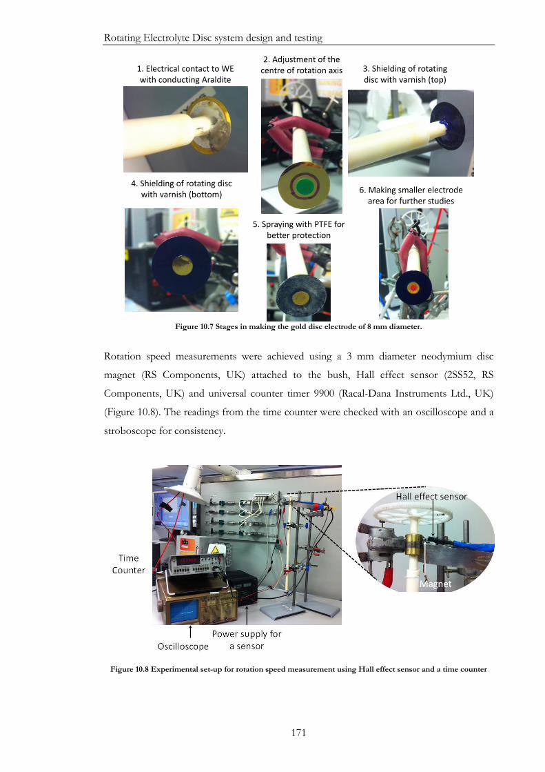
Rotating Electrolyte Disc system design and testing
171
Figure 10.7 Stages in making the gold disc electrode of 8 mm diameter.
Rotation speed measurements were achieved using a 3 mm diameter neodymium disc
magnet (RS Components, UK) attached to the bush, Hall effect sensor (2SS52, RS
Components, UK) and universal counter timer 9900 (Racal-Dana Instruments Ltd., UK)
(Figure 10.8). The readings from the time counter were checked with an oscilloscope and a
stroboscope for consistency.
Figure 10.8 Experimental set-up for rotation speed measurement using Hall effect sensor and a time counter
1. Electrical contact to WE with conducting Araldite
2. Adjustment of the centre of rotation axis 3. Shielding of rotating
disc with varnish (top)
4. Shielding of rotating disc with varnish (bottom)
5. Spraying with PTFE for better protection
6. Making smaller electrode area for further studies

Rotating Electrolyte Disc system design and testing
172
10.3.2. RED measurements in aqueous system
The RED setup was applied to study the mass transfer characteristics of the Fe3+/ Fe2+
redox reaction in solutions of ferrous and ferric chloride of various concentrations in
acidified 1 and 3 M KCl medium initially using a platinum and later gold disc electrodes.
An equimolar solution of ferrous and ferric chloride (0.014 M) with 3 M KCl as supporting
electrolyte and a platinum disc electrode (WE) on the base of YSZ disc were investigated.
Platinum wire and piece of platinum mesh were used as the counter electrode (CE) and a
saturated calomel electrode (SCE) was employed as a reference electrode (RE). The
potential difference of SCE measured vs. reversible hydrogen electrode (RHE) was
measured to be 0.249 V. The area of the platinum working electrode was 0.28 cm2.
Note that ferric and ferrous chlorides were chosen as analogues to potassium ferri and
ferro cyanides (K3Fe(CN)6 and K4Fe(CN)6) that are typically used in standard RDE
measurements185 but were avoided here due to their hazardous nature. The supporting
electrolyte186 was a solution of 3 M potassium chloride in deionised water, containing 0.014
M of ferric chloride and ferrous chloride. Oxygen in the cell was purged by firstly bubbling
nitrogen through the solution and then continuously blanketing the solution with a
constant flow of nitrogen throughout the experiment. Rotated disc voltammograms
(Figure 10.9) were obtained using various rotation speeds at room temperature. Applying
the linear sweep voltammetry technique the potential was swept from -0.4 V up to +1.4 V
versus SCE with a scan rate of 10 mV s-1. The system was operated at progressively
increasing rotation speeds. The estimated accuracy of currents measurements is ± 10 µA.
Figure 10.9 LSVs with increasing rotation rate for the ferrous-ferric redox couple using 0.014 M Fe2+ /0.014M Fe3+ in 3M KCl (data obtained via 6 mm Pt disc electrode).
The obtained data (see Figure 10.9) show that the developed design for RED setup
conforms to standard RDE behaviour, indicating a limiting current density which increased
with rotation speed, ω, in both the anodic and cathodic sweeps. Next, having developed the
method for rotation speed measurement, the above experiment was repeated using a
-0.2 0.0 0.2 0.4 0.6 0.8 1.0 1.2
-20
-10
0
10
20
Applied potential vs SCE / V
Cu
rre
nt
de
nsity /
mA
cm
-2

Rotating Electrolyte Disc system design and testing
173
solution of ferrous and ferric chloride in acidified 1 M KCl solution using a gold disc
electrode (8 mm diameter) (Figure 10.10). In place of the SCE reference, a dipping
platinum wire was used so that potentials were measured versus the equilibrium potential
of the ferrous-ferric couple pertaining in each solution. This reference was simple and
convenient with no junction potential; it operated most successfully and had the unusual
feature that all sweeps showed a zero current at zero applied potential versus the platinum
RE.
Figure 10.10 Cyclic voltammograms for a range of rotation rates for the ferrous-ferric redox couple using 0.02 M Fe2+ / 0.02 M Fe3+ (a) and 0.02 M Fe2+ / 0.002 M Fe3+ in 1M KCl plus 0.01 M HCl (b) (data obtained via 8 mm Au disc electrode). The reference electrode was a dipping platinum wire so that potentials shown were versus
the equilibrium potential of the particular ferrous-ferric couple under investigation.
The rapid increase in current at potentials of ≥+0.4 V potential in Figure 10.10a indicates
the onset of O2 evolution. Sweeps in the negative-going direction did not reach potentials
at which hydrogen is evolved (-0.77 V for equimolar concentrations of Fe2+ and Fe3+).
Flatter positive-going voltammograms were achieved when the concentration of Fe2+ was
reduced as shown in Figure 10.11a, b and these data were used for analysis in respect of
this ion.
Figure 10.11 Cyclic voltammograms for a range of rotation rates for the ferrous-ferric redox couple using 0.002 M Fe2+ / 0.02 M Fe3+ in 1M KCl plus 0.01 M HCl (a); expanded view (b) (data obtained via 8 mm Au disc
electrode). The reference electrode was as for Figure 10.10.
Diffusion coefficients for Fe2+ and Fe3+ were determined from Levich plots (Figure 10.12).
-0.6 -0.4 -0.2 0.0 0.2 0.4 0.6
-8
-6
-4
-2
0
2
4
6
8
10
12
14
Applied potential (V)
Cu
rrent density (
mA
cm
-2)
5.81 Hz (349 rpm) 8.26 Hz (495 rpm)
11.5 Hz (691 rpm) 16.7 Hz(1002 rpm)
(a)
-0.6 -0.4 -0.2 0.0 0.2 0.4 0.6
-2
0
2
4
6
8
10
(b)C
urr
ent density (
mA
cm
-2)
Applied potential (V)
4.58 Hz (275 rpm) 8.30 Hz (498 rpm)
12.1 Hz (724 rpm) 15.4 Hz (926 rpm)
18.8 Hz (1126 rpm)
-0.6 -0.4 -0.2 0.0 0.2 0.4 0.6
-10
-5
0
5
10
15
Cu
rre
nt
de
nsity (
mA
cm
-2)
Applied potential (V)
3.53 Hz (212 rpm) 6.13 Hz (368 rpm)
8.20 Hz (492 rpm) 10.2 Hz (612 rpm)
13.6 Hz (816 rpm) 18.9 Hz (1135 rpm)
(a)
0.0 0.1 0.2 0.3 0.4
-0.4
-0.2
0.0
0.2
0.4
0.6
0.8
1.0
(b)
Cu
rre
nt
de
nsity (
mA
cm
-2)
Applied potential (V)
3.53 Hz (212 rpm) 6.13 Hz (368 rpm)
8.20 Hz (492 rpm) 10.2 Hz (612 rpm)
13.6 Hz (816 rpm) 18.9 Hz (1135 rpm)

Rotating Electrolyte Disc system design and testing
174
Figure 10.12 Plots of limiting current density for Fe3+ reduction (a) and Fe2+ oxidation (b) vs. square root of rotation speed.
The diffusion coefficients for Fe3+and Fe2+ were calculated from the slopes of the Levich
plots to be 4.4 × 10⁻⁶ and 5.8 × 10⁻⁶ cm2 s-1respectively, which are similar to those reported
by Spiro and Creeth187(see Table 10.1). The standard error in the diffusion coefficient data
is estimated to be ±10%. The correlation with literature values is satisfying, though in this
work, RDE measurements in aqueous systems were made to validate the apparatus and not
to obtain definitive values of the diffusion coefficients.
Table 10.1 Comparison of diffusion coefficients for Fe2+ and Fe3+ ions with literature.
UCL132(present work) Spiro and Creeth187 D(Fe3+)/10-6 (cm2 s-1) 4.45 4.86 D(Fe2+)/10-6 (cm2 s-1) 5.81 5.78 Medium (mol dm-3) 1 M KCl, 0.01 M HCl 0.05 M HClO4
10.4. Application of RED to LME SOFCs
10.4.1. Construction of RED for LME SOFCs
Construction of RED setup for high temperatures was based on the design shown in
Figure 10.3 (Design 2) and the previous setup for aqueous systems (Figure 10.6). Some
parts used in the RED for aqueous study were replaced by thermally stable materials. As
such, the disc at the bottom could not be glued with epoxy resin (stable up to 200 °C) and
was replaced by high temperature ceramic cement (Ceramabond 552, Aremco Products,
USA).
Electrical connection to the rotating electrode was complicated by the third alumina tube
(tube 3, Figure 10.3) placed inside the rotating tube for supply of air to electrode surface. If
the Pt wire were to run all the way through the inside of the rotating tube (tube 2, Figure
10.3) as in the case of RED for the aqueous system, the wire would also rotate and as a
result would wrap around the stationary central tube causing it to break.
0 2 4 6 8 10 12
0
1
2
3
4
5
6
7
8
ilim
cathodic
at -0.4 V
/ (rad sec-1)1/2(a)
i lim / m
A c
m-2
0 2 4 6 8 10 12
0.0
0.2
0.4
0.6
0.8
1.0
ilim
anodic
at 0.2 V
i lim / m
A c
m-2
/ (rad sec-1)1/2(b)

Rotating Electrolyte Disc system design and testing
175
To avoid this it was decided to engineer a platinum track on the outer side of rotating tube;
Pt ink was painted along and inside a groove in the alumina tube which was cut with a
diamond tipped drill. Connection from the bottom disc to the track was made with Pt wire.
Electrical connection at the top (to a brass bush) was made by fixing one end of Pt wire to
the Pt track and other end to the bush. Connection of the wire to the track at the top of
the tube was made with conducting adhesive (silver loaded Araldite, RS Components, UK).
The constructed RED set-up based on Design 2 for LME SOFC is shown in Figure
10.13(a). Once assembled the RED apparatus was used in a LMA SOFC cell at 770 °C as
shown in Figure 10.13 (b).
Testing of the RED in LMA SOFC resulted in several problems that were due to
constraints in the size of furnace and poor sealing of the electrolyte disc to the bottom of
the rotating tube. From one aspect, the furnace used in the first instance enabled the
application of relatively small (19 mm outer diameter) and hence less expensive YSZ tube
that contained the RED immersed into liquid tin (Figure 10.3). However, from the other
aspect, the small size of the furnace gave very little flexibility and generated unfavourable
conditions of liquid flow around the disc, which upon rotation may lead to formation of
vortices that may introduce distortion to the liquid flow108,109,186. Once tin was molten, the
RED was inserted inside the YSZ tube, which caused cracking of the latter due to thermal
shock. In addition, gas tight sealing of the YSZ disc at the bottom of rotating alumina tube
was not achieved. This was probably due to mismatch of thermal expansion coefficients
between 8YSZ (11 × 10-6/ °C) and alumina (8.4 × 10⁻⁶/ °C), which resulted in a porous
seal.
To resolve practical challenges, a larger furnace was purchased and this has opened up new
possibilities in designing the latest system. The new design aimed to address disadvantages
from Design 2 and also to take into account technical problems arisen from initial testing
of RED in LMA SOFC.

Rotating Electrolyte Disc system design and testing
176
Figure 10.13The ready RED set-up in operation of LME SOFCs.
10.4.2. Final design for RED for LME SOFCs
The latest design (Design 3) is shown Figure 10.14 and its rationale in comparison with
Design 2 (Figure 10.3) is summarised as follows.
Figure 10.14 The latest design of RED - Design 3.
(a) (b)
air in
electronic contacts to Sn
tube 3 - Al2O3 (stationary)tube 1 - YSZ (rotating)
Argear wheel
porous Pt electrode
carbon brush
silica tube
tube 2 - Al2O3
(stationary)
Sn(l)
pyrophyllite cap
gear motor
YSZ disc
Pt electrodes
brass bushAl2O3 collar
O2
CE
RE
Glass seal
YSZ disc
WE SE

Rotating Electrolyte Disc system design and testing
177
Application of a larger furnace allowed the use of a larger container (silica instead of
zirconia having an advantage in terms of cost) for tin and the RED minimising edge effects
regarding the hydrodynamics, as well as turbulence of the flow.
The second major change in Design 3 was replacement of the rotating tube material from
alumina to YSZ in order to eliminate thermal expansion difference of the two components
(tube and disc) and should prevent breakage of the seal. A glass-ceramic sealant has been
sourced to replace the ceramic cement, which may improve the sealing and resolve the
sealing problem.
The possibility to pump oxygen in/out of tin is proposed via application of the same YSZ
rotating tube to avoid use of an extra YSZ tube that would have been immersed into the
liquid metal for pumping of oxygen into and out of the tin.
Another important improvement of the latest design is the placement of the reference
electrode within the WE disc. Also, a second electronic contact to tin is proposed to be
used for sensing the electrode connections. This will eliminate any ohmic drop in the
current collector that is in contact with the tin.
Electrical connections from the electrodes coated on the inner side of the rotating YSZ
tube (for oxygen pump) and from the YSZ discs (from CE and RE) require four brass
bushes and four carbon brushes that are electrically isolated from each other. Note that the
glass-ceramic seal employed between the YSZ disc and YSZ tube will totally isolate
pumping and working electrodes from each other. Work is underway to construct the RED
apparatus based upon Design 3.
10.4.3. Electrochemical system for RED studies
It is suggested that the assembled RED system should be tested in the following system to
explore mass-transport and kinetics processes within the liquid tin anode SOFC:
(Working Electrode) (H2)/Ar, [O]Sn| LMA|YSZ, Pt, air (Counter Electrode)
Following the latest design of RED, the potential applied via the pumping electrode sets
the concentration of dissolved oxygen, [O]Sn, in tin. Counter and reference electrodes (Pt air
electrodes) are painted on the inner surface of the rotating electrolyte disc in accordance
with the latest design.
Oxygen is pumped in/out of the system to maintain the concentration of oxygen in tin at a
fixed value and below the solubility limit, and so prevent oxidation of liquid tin to tin oxide
or dioxide in the bulk. This is achieved by using rotating YSZ tube as oxygen pump with Pt
electrode painted on its inner side and liquid tin electrode on its outside (Design 3; Figure

Rotating Electrolyte Disc system design and testing
178
10.14). For similar reasons, argon will be blown into the silica container to keep the O2
level very low.
Having examined oxidation of H2 and water dissociation in LMA SOFCs (see Chapters 7-
9), the assembled RED set-up is intended to investigate kinetics and mass-transport of
either anodic injection of oxygen (as part of oxidation of H2 in LTA SOFC) or cathodic
oxygen reduction (in case of water dissociation) reactions as shown in Equation (10.1).
𝑂2− [𝑂]𝑆𝑛 + 2𝑒− (10.1)
It is planned to operate the system in a narrow potential window whereby formation of tin
oxide is eliminated (mode CE). The measurement of the diffusion coefficient of dissolved
oxygen is anticipated. The determination is important as it will be obtained via a direct
method rather than an indirect one as applied by Abernathy et al.6
10.5. Conclusion
A novel rotating electrolyte disc (RED) has been proposed as an inverted Rotating Disc
Electrode (RDE) technique where a solid electrolyte disc rotates in a liquid electrode, as
opposed to a solid electrode rotating in a liquid electrolyte. This unique apparatus is being
developed for examination of transport properties and mechanisms within the liquid metal
anode. The oxidation of hydrogen and/or electrolysis of water observed in LMA SOFC are
proposed for examination via RED. In particular, the anodic injection of oxygen and
cathodic extraction/ reduction of oxygen are two reactions to be quantified by applying
RDE theory.
Prior to construction of the RED apparatus, various designs were suggested and
progressively improved. Once the finalised design for RED was proposed, the engineering
aspects of RED were tested in a simple aqueous system. For that, a modified version of
RED was built and tested in an electrochemical system with ferrous and ferric chloride
solutions in KCl electrolyte media. The obtained data show that the developed design
conforms to standard RDE behaviour (increasing rotation speed ω increased the observed
limiting current density). The diffusion coefficients for Fe3+ and Fe2+ were calculated from
the slopes of the Levich plots to be 4.4 × 10⁻⁶ and 5.8 × 10⁻⁶ cm2 s-1 respectively, which are
similar to literature values.
Having been tested in aqueous system, the RED was constructed according to Design 2
and tested in LMA SOFC. Electrochemical data could not be obtained due to technical
problems arising from imperfections of Design 2 and also some practical issues, such as
poor sealing between the YSZ disc and alumina tube. This and other disadvantages have

Rotating Electrolyte Disc system design and testing
179
been addressed in the latest design of RED. The full details of the final design are outlined,
and the construction of the RED in accordance with it is in progress.

Conclusion and future work
180
11. Conclusion and future
work This thesis presents experimental findings from operation of liquid metal anode solid oxide
fuel cells (LMA SOFCs) fuelled with hydrogen in Electrochemical-Chemical (EC) and
Chemical-Electrochemical (CE) modes, as well as on operation of a reverse SOFC with
liquid metal electrode for water electrolysis. A novel Rotating Electrolyte Disc (RED)
technique is proposed to provide fuller understanding of the fundamental operation of
LMA SOFCs. Initial results, including the testing of RED in an aqueous electrochemical
system are discussed. This section summarises the main contributions of the obtained
results.
11.1. Conclusion
There is growing awareness of the detrimental consequences of carbon dioxide emissions
that drives development of environmentally friendly technologies for power generation
from fossil fuels. LMA SOFCs offer the possibility of direct and highly efficient
electrochemical conversion of solid fuels into electrical energy, with reduced levels of pure
CO2 (not diluted with NOx gases). As an alternative to conventional power generating
technologies, the LMA SOFC fuelled with hydrogen has been considered in this study. The
use of hydrogen is considered as a model system for studying this technology to provide a
basis for studies involving solid carbon fuel.
This novel type of solid oxide fuel cell with liquid metal electrodes (anodes) has the
advantage of greater fuel tolerance, the ability to operate on solid fuel as well as to perform
in battery mode in case of temporary fuel starvation. A range of metals have been reviewed
including tin, the anode material on which most research has been performed. The key
concepts of this technology are discussed along with the open research challenges that need
to be addressed for its scale-up and commercialisation. Despite numerous studies,
understanding of the reaction kinetics at the liquid metal-fuel and liquid metal-electrolyte
interfaces, as well as oxygen diffusivity through the liquid metal layer, needs further
systematic investigation.
Electrochemical cells, and a workstation developed for electrochemical characterisation of
LMA SOFCs, have been developed and tested and investigation of the ionic conductivity

Conclusion and future work
181
of the solid electrolyte chosen for this project (yttria-stabilised zirconia) has been made.
First, potentiometric measurements using 10 mol.% yttria-stabilised zirconia (10YSZ)
symmetrical cells as an oxygen sensor resulted in close agreement between measured and
calculated concentration of oxygen for the applied range of gas flow rates. Then a series of
linear sweep voltammetries from -1.0 to 1.0 V for temperature range (500 - 800 °C) yielded
current-voltage curves whereby the conductivity for 10YSZ increased progressively up to
800 °C (this included the overpotential on Pt electrodes). Lastly, the precise determination
of YSZ ionic conductivity was performed using the Electrochemical Impedance
Spectroscopy (EIS) technique. The EIS spectra showed substantial reduction in bulk
resistance of electrolyte in agreement with the Arrhenius relationship. Ionic conductivity of
6 mol.% YSZ at 1000 °C was calculated to be 6.58 × 10⁻² S cm-1 which was in agreement
with reported value of 6.67 × 10⁻² S cm-1 for 7.5 mol.% YSZ. These results assisted in
evaluating the electrolyte based on mechanical and electrical properties. As a result, the
original 6mol.% YSZ electrolyte was replaced with the more conductive 8 mol.% YSZ
electrolyte.
Measurements of open circuit potential as a function of temperature for liquid tin anode
SOFC (operated in battery mode) resulted in close agreement with thermodynamic
predictions. This result confirmed the validity of the workstation and cell components
required for testing of LMA SOFCs. Another outcome was the validation of the use of a
glassy carbon rod as a current collector from liquid tin, which remained inert and had no
alloying/ corrosion issues throughout numerous experiments.
An optimisation of the workstation was performed to investigate and minimise inevitable
leak of oxygen into the LMA SOFC system. Experimental work involved the measurement
of permeation rates of air (oxygen) through plastic tubing incorporated in the developed
experimental rig. The concentration of leaked oxygen was found to be inversely
proportional to the gas flow rate. Apart from oxygen that leaked from ambient air,
additional pumping of oxygen was made using the YSZ oxygen pump. The amount of
pumped oxygen was found to be consistent with Faraday’s law, which confirmed reliability
and accuracy of the electrochemical oxygen pump. Parasitic ingress of oxygen decreased
upon reduction in the length of silicone peroxide tubing and later via its complete
replacement with hard nylon tubing. A methodology to account for the effect of oxygen
leakage into the fuel cell on the overall current was also developed. It was found that about
57% of the pumped current (translated to oxygen) is attributed to the change in fuel cell
reduction current. The developed technique was an important step that allowed the effect

Conclusion and future work
182
of leaked oxygen to be separated from other processes occurring in the liquid tin anode.
This practice was successfully utilised throughout the whole study.
Followed by the experimental optimisation, a classification for the mechanisms for
oxidation of gaseous fuel (hydrogen) in liquid metal anode SOFCs depending on the
reaction conditions was described in Chapter 6. The proposed mechanisms are suggested
to be true for all metal anodes associated with formation of solid metal oxide upon
polarisation. Four different modes of operation (and hence mechanisms for oxidation)
were identified: direct electrochemical oxidation of fuel gas at the liquid metal anode/ YSZ
interface (E mode); homogeneous oxidation of fuel in the bulk of the liquid anode by
dissolved oxygen, followed by electrochemical injection of oxygen to replace the consumed
oxygen (CE mode); electrochemical oxidation of liquid metal at the anode/ electrolyte
interface, followed by chemical oxidation of fuel by metal oxide in the bulk of the metal
(Electrochemical-Chemical mode 1 (EC1)); and electrochemical oxidation of liquid metal at
a rate significantly higher than metal oxide reduction with fuel, which may lead to the
formation of a blocking metal oxide layer (Electrochemical-Chemical mode 2 (EC2)).
Operation of a liquid tin anode SOFC in the commonly applied EC modes was performed.
The obtained polarisation curve resulted in a “turning point” on the potential axis, beyond
which the current density reduced dramatically and hence the fuel cell performance
dropped. The decline in current density was attributed to the formation of a blocking layer
of SnO2 at the liquid tin / electrolyte interface. The findings from the polarisation curve
were in agreement with reported studies. This result pointed to the requirement for a study
where operation was in a potential region in which there was no formation of tin oxide,
which entails E/ CE modes as the only possibilities. This enables the elimination of
formation of the blocking layer and investigation of significant parameters for fuel
oxidation within the liquid metal anode.
The oxidation of hydrogen in LMA SOFCs was examined in Chapter 7. Steady anodic
currents were essentially proportional to hydrogen partial pressure and independent of total
gas flow rate. Two models were considered for either (i) direct anodic oxidation of
dissolved hydrogen (E mode) or (ii) homogeneous reaction between dissolved hydrogen
and oxygen, followed by anodic injection of oxygen to replace that removed by the
chemical reaction (CE mode). The former model was rejected as it required the
incorporation of the hydrogen / argon fuel gas in the form of a persistent foam which was
not detected. The latter model was validated using steady-state and dynamic
experimentally-generated data and resulted in the evolution of the parameter z. This
parameter, termed the dynamic oxygen utilisation coefficient, does not have fundamental

Conclusion and future work
183
significance but is likely to be of technological importance when designing LMA SOFC
reactors. It is shown that 𝑧 parameter is closely related to the Damkohler number which
compares the rates of chemical reaction and mass-transfer in the process.
The model for CE mode was further validated in Chapter 8. For that, a method termed
anodic injection coulometry (AIC) was proposed and developed to determine the
parameter 𝑧, which depends upon geometric (electrode area and volume of tin), mass-
transfer (diffusion layer thickness and diffusion coefficient of dissolved oxygen) and kinetic
factors in the cell. The LMA SOFC was operated in two regimes, whereby anodic injection
of oxygen at the liquid tin / YSZ interface was measured with time at a fixed applied
potential (after a specific period of hydrogen dissolution at open circuit). The potential of
the liquid tin was chosen to be close (within 10 mV) to the equilibrium potential of the
Sn/SnO2 couple. At this potential the oxygen concentration is expected to be close to the
saturated value, as moving to more positive potentials would result in precipitation of
SnO2. Theoretical treatment of the coulombic anodic injection charge from each regime
enabled the value of 𝑧 to be determined and was found to 0.83 for hydrogen partial
pressure of 16 kPa; it also enabled a measurement of oxygen solubility in liquid tin at 780
°C of 0.10 at.% to be made. The obtained value was found to be similar to literature
values. The estimated uncertainty on 𝑧2 value is 3.5 % (i.e. 𝑧2 =0.83 ± 0.03).
A novel concept for water (steam) electrolysis using the liquid metal electrode solid oxide
system is demonstrated in Chapter 9. It is suggested that water dissolves in the tin
whereupon it dissociates into hydrogen (which is carried away in the inert gas stream) and
dissolved oxygen in monoatomic form. This increases the dissolved oxygen concentration
which drives cathodic oxygen extraction. Initial experimental data showed that measured
current-time curves followed an exponential function with time constants slightly higher
than ones measured for hydrogen oxidation (followed by anodic injection of oxygen). More
experimental and modelling work is required to fully understand the operation of reverse
LMA SOFCs for water electrolysis.
The experimental and modelling work presented so far has clarified the behaviour of the
oxygen-hydrogen/water tin system in the ‘inert window’ and provided a firm basis for
proceeding with studies via the Rotating Electrolyte Disc (RED).
The final part of this study presents the development of a novel Rotating Electrolyte Disc
(RED) technique for determination of parameters controlling mass transport of dissolved
oxygen (and /or other gases) and oxidised species including metal oxide in the liquid metal;
the technique also provides the possibility for investigation of heterogeneous and
homogeneous reaction kinetics, as well as the influence of electrode contaminants. In the

Conclusion and future work
184
proposed design, a solid electrolyte disc rotates in a liquid metal electrode (e.g. tin), as
opposed to a solid electrode disc rotating in a liquid electrolyte, making this concept
unique. Evolution of designs for novel RED apparatus and construction for high
temperature studies is presented. In order to demonstrate the validity of the concept and
design for high temperature systems, the engineering aspects of the RED apparatus were
tested in an aqueous electrochemical system (equimolar solution of ferrous and ferric
chloride with KCl as supporting electrolyte and a gold disc electrode on the base of the
zirconia disc). The obtained data show that the developed design conforms to standard
RDE behaviour (increasing rotation speed ω increased the observed limiting current
density).
The diffusion coefficients for Fe3+ and Fe2+ as calculated from the slopes of the Levich
plots were found to be 4.4 × 10⁻⁶ and 5.8 × 10⁻⁶ cm2 s-1 respectively, which are similar to
those reported in the literature. The standard error in the diffusion coefficient data is
estimated to be ±10%. The model system for application of RED for investigation of LME
SOFCs has been discussed.
11.2. Recommendations for future work
This project has been aimed at understanding the mechanisms of operation in liquid metal
anode solid oxide fuel cells (LMA SOFCs). Options for future work in this area are split
into three phases: short-term, medium-term and long-term.
In the short-term, construction of the rotating electrolyte disc (RED) apparatus
based upon the latest design, proposed in this study, can be done. This work involves three
main aspects: sealing of the rotating electrolyte disc affixed to the bottom of rotating tube,
development of electrical connection from three electrodes system and construction of
mechanical parts that enable rotation of the RED setup in liquid tin up to 1800 rpm at
temperatures >700 °C.
This work is followed by application of built RED apparatus for studies in LMA SOFCs.
This encompasses experimental work on oxygen reduction reaction at rotating
electrolyte/liquid tin interface at various rotation speeds. The concentration of oxygen can
be set via the potential applied to the liquid tin electrode, while the diffusion layer thickness
is fixed via rotation speed. Applying the Levich, Koutecki-Levich analysis it is possible to
elucidate mass transport (diffusion coefficient of dissolved oxygen) and kinetic (if any)
parameters for the oxygen reduction reaction.
The next step in the application of the RED can be done in the model system developed in
this thesis (Chapters 7 and 8), whereby oxidation of hydrogen takes place in an LMA
SOFC operated in mode CE. The data generated with the RED can be compared to

Conclusion and future work
185
previous data from a stationary system. Most importantly, the results will provide an insight
into the mechanisms underpinning transport and kinetic phenomena within the liquid
metal anode during the fuel oxidation process. The measurement of diffusion coefficient of
dissolved oxygen can be compared to the one found in the step above and ideally should
remain constant.
The work outlined above may take six months and requires only one PhD student.
The medium-term work is outlined as follows and would require a team of up to
a dozen researchers. The time scale for a medium-term work may be up to five-six years.
The first step would be the optimization of an existing workstation built for stationary
electrochemical testing of LMA SOFCs. One of the challenges in this study was parasitic
ingress of oxygen into the fuel cell despite substantial improvement of the rig, such as
replacement of silicone tubing with impermeable nylon tubing. Therefore it is essential to
replace all plastic tubing with stainless steel tubing and most importantly to apply stainless
steel joints, valves, etc. In addition the supplied fuel (gaseous mixture of inert gas and fuel)
should be passed through a titanium furnace to reduce the oxygen level down to few (ca. 5-
10) ppm.
The optimization of the workstation should be followed by further experimental work on
hydrogen oxidation in LMA SOFCs in CE mode (as described in Chapters 7 and 8) at
various operating potentials (less positive than -0.90 V vs. RE employed in this study). This
can be done in order to examine the effect of potential on the time-constants and test the
validity of the model in wider potential range. In addition, it would be interesting to alter
the geometry of the cell (e.g. electrode area and tin volume) to see if the value of dynamic
oxygen utilization coefficient is consistent with predictions from the CE model.
In addition, variation in the operating temperature and applied potential (further away or
closer to the Sn/SnO2 equilibrium potential) may potentially result in the range of oxygen
solubility measured with greater accuracy than the one in this work, as this time the oxygen
leakage will be reduced to minimum.
The following step should involve improvement of the current electrochemical model for
CE mode including refinement of the assumption on identification of the rate-determining
step in hydrogen oxidation process. In the present model this assumption was made
because the supplied fuel was dry (i.e. contained only traces of water) and hence the
backward reaction (water reduction) was ignored. This assumption may not be absolutely
true and in order to investigate it additional work with humidified hydrogen can be done.
Combining the results from both models (hydrogen oxidation in CE mode and water
electrolysis) should result in a model with more defined boundary conditions.

Conclusion and future work
186
The basis of an improved model can be applicable for modelling of a more complicated
system involving other gaseous fuels (e.g. carbon monoxide) which are of practical interest.
A model that incorporates oxidation of carbon monoxide instead of hydrogen should be
developed in conjunction with practical work on evaluation of the performance of LMA
SOFC with other fuels such as carbon monoxide and solid carbon.
Large deposits of coal worldwide provide a niche for this technology in the global market,
particularly in the coal-dependent countries. With regards to fuel cell testing using solid
carbon, the effect of carbon particles size on the performance should be evaluated.
Greater attention is needed to explore one of the benefits of this technology – anode
tolerance to fuel impurities59. Initial studies may involve evaluation of LMA performance in
presence of common contaminants (e.g. sulphur), which according to the literature should
electrochemically oxidise in the bulk of liquid anode and serve as additional energy source
(acting as a fuel).
Application of carbonaceous fuels (gaseous or solid) requires the analysis of the gas outlet
from the fuel cell using the gas chromatographer or mass spectrometer. This would
provide additional information concerning the kinetics of the reduction of dissolved
oxygen and /or metal oxide and enable their comparison with the anode oxidation kinetics.
It would also allow the practical efficiency of the fuel oxidation processes with both solid
carbon and gaseous CO to be measured.
In addition to a tubular design (applied in the present work), a pellet cell design can be
introduced to perform electrochemical characterisation of LMA SOFCs. In such a design,
a thin electrolyte pellet is affixed to the bottom of zirconia tube with high temperature,
non-porous sealant. Once in-situ electrochemical characterisation has been made, the pellet
can be dismantled from the supporting tube and be exposed to further ex-situ physical
characterisation. Analysis of Sn|SnO2|YSZ interphases using scanning electron
microscopy along with energy-dispersive X-ray spectroscopy (EDX) would provide more
detailed information on structure of the electrodes, formation of a blocking layer, etc.
compared to the previously applied tubular cell.
In parallel to studies on oxidation of fuel in chemical –electrochemical (CE) mode, the
operation of LMA SFOCs in common in literature electrochemical –chemical (EC) modes
is appropriate.
The application of the electrochemical impedance spectroscopy (EIS) may be particularly
interesting to differentiate various losses in the LMA SOFC operated in both CE and EC
modes. The EIS data on operation of LMA SOFC in EC modes has been measured
previously; however, no EIS data is available for LMA system operating in the CE mode.

Conclusion and future work
187
Development of a model for EC modes would be valuable, as it may generate additional
parameters to be taken into consideration for design of LMA SOFCs with improved
performance.
Electrolytic performance of liquid metal electrode systems can be of practical interest.
Further experimental work is required on water (steam) electrolysis using the liquid metal
electrode. In particular, a wider partial pressure range of water should be applied (using the
heated lines) with minimal inclusion of parasitic oxygen to investigate the mechanism for
water electrolysis. If initial studies show promising results, further exploration of two liquid
metal electrodes (cathode and anode) for steam electrolysis and fuel oxidation (similar to
conventional solid oxide steam electrolysers) can be made. It is optional to examine water
electrolysis and may not be part of this work plan as the main focus of this study is fuel cell
operation.
Once fundamental data on mechanisms and transport properties of LMA SOFCs are
obtained in work under short term and medium term time scale, their implication for the
scale-up of the technology would be appropriate. The obtained findings should
complement the development of commercial cells and stacks. For that the development of
multi-scale and multi-physics models (using COMSOL software, for example) can be
undertaken. Thermal imaging technique may be applied additionally for examination of the
heat transfer process.
The long-term goals for an improved development of LMA SOFC technology include
development and testing of LMA SOFC stacks, techno-economic analysis of LMA SOFC
stacks in terms its performance, capital and maintenance costs. One of the biggest
challenges in the development of the stacks might be the poor wetting properties of tin. In
the present study, only large volume of molten tin anode was used. Therefore an
optimization work would be necessary to identify the optimum thickness of liquid anode,
as well as conditions at which its surface tension is the lowest.
As such, for successful implementation of LMA SOFCs, its economics has to be
competitive with existing mature technologies (e.g. power plants). Therefore, analysis of the
capital costs of stack manufacture, maintenance costs and future electricity costs will provide a
basis for improvements to the design of LMA SOFCs. At later stages trialing of the pilot
plant with built LMA SOFC stacks can be made. The rough estimate on the time frame
for long-term is about 20 years.

Nomenclature
188
Nomenclature Parameters
and Variables
Description Section
a (a) Rate of electrochemical oxidation of metal to metal oxide
6.2
(b) Tafel equation constant 2.2.4 ai Activity of a specie i 2.2.3 as Specific external surface area of the catalyst pellet in
Equation(7.55)/m2(kgcat)-1
7.6
Intercept (concentration of O2 in the carrier gas, N2) 5.2.1
A (a) Are of reaction interface/ cm2 7.4 (b) Disc electrode surface area/ cm2 3.4.4 (c) Cross-sectional area of component i / cm2 2.2.4 (d) Area of permeable membrane / cm2 5.2 b (a) Rate of chemical reduction of metal oxide to metal 6.2 (b) Tafel equation constant 2.2.4 c’ Concentration of hydrogen in the bulk of the melt / mol cm-3 7.4 c’
1 Steady value of c’ at p’1 Appendix C
c’2 Steady value of c’ at p’
2 7.4 c’
3 Steady value of c’ at p’3 Appendix C
c’’ Concentration of water in the bulk of the melt / mol cm-3 9.3.3
𝑐 a) Concentration of oxygen in the bulk of the melt / mol cm-3 7.6
b) Concentration of leaking oxygen / ppm 5.2.1
𝑐1 Steady concentration of oxygen in the bulk of the melt at p’1 /
mol cm-3 7.6
𝑐2 Steady concentration of oxygen in the bulk of the melt at p’2 /
mol cm-3 7.6
𝑐3 Initial concentration of oxygen after switch from OC to potential, E / mol cm-3
8.4.1
𝑐∗ Saturated concentration of oxygen at potential E in the bulk of the melt at p’=0 / mol cm-3
7.6
𝑐∗∗ Equilibrium concentration of dissolved oxygen at potential E in the bulk of the melt at p’’=0 / mol cm-3
9.3.3
c*’ Saturated concentration of hydrogen in the bulk of the melt / mol cm-3
Appendix C
c*’1 Saturated concentration of hydrogen in the bulk of the melt at
p’1 / mol cm-3
Appendix C
c*’2 Saturated concentration of hydrogen in the bulk of the melt at
p’2 / mol cm-3
7.4
𝑐 The difference between the equilibrium oxygen concentration at potential E and concentration in the bulk (Equation 9.16)
9.3.3
𝑐1 The value of 𝑐 at 𝑝′′ = 𝑝1′′ 9.3.3
𝑐2 The value of 𝑐 at 𝑝′′ = 𝑝2′′ 9.3.3
C Concentration of analyte in bulk solution / mol cm-3 3.4.4 D Diffusion coefficient / cm2 s-1
Diffusion coefficient of oxygen in the melt/ cm2 s-1 7.6
D’ Diffusion coefficient of hydrogen in the melt / cm2 s-1 7.4

Nomenclature
189
Da Damkohler number 7.6 DaII The second Damkohler number 7.6 E Potential / V Ea Activation energy for conduction/ kJ mol-1 4.2.1 Ecell Cell potential / V 2.2.4 EN Nernst Potential / V 2.2.3 Erev Reversible potential / V 2.2.2 f Frequency / number of revolutions per second 3.4.3 F Faraday’s constant / 96,485 C mol-eq-1 2.2.2 ΔG Total Gibbs free energy change / J mol-1 2.2.2 ΔGr0 Gibbs free energy change of reaction / J mol-1 2.3.2 ΔG0
M-MOn Gibbs free energy for metal oxidation reaction
(M+ (n/2)O2 MOn)
2.3.2
ΔH Total Enthalpy of reaction /J mol-1 2.2.2 i Anodic oxidation or cathodic reduction current / mA icathodic Parasitic oxygen reduction current / mA 7.3.1 id Diffusion-controlled current / A (Equation (3.6)) 3.4.4 ik Kinetic current / A 3.4.4 i1 Steady anodic current at p’
1/ mA 7.4 i2 a) Steady anodic current at p’
2 / mA 7.4 b) Steady cathodic current at p’’
2 / mA 9.3.3 i3 Initial (maximum) anodic current after switch from OC to
potential, E/ mA 8.4.1
I Pumped current / A 5.2.1 I(m) Amplitude of current sinusoidal oscillation / A 3.4.3 I(t) Current sinusoidal oscillations / A 3.4.3 j Current density / A cm-2 2.2.4 j0 Exchange current density / A cm-2 2.2.4 jlim Limiting current density / A cm-2 2.2.4 J Permeation rate (flux) of gas through a membrane / cm3 s-1 5.2
𝐽 Flux of oxygen in the melt /mol s-1 7.6
J’ Flux of hydrogen in the melt /mol s-1 7.4 k Boltzmann constant / J K-1 4.2.1 kf a) Rate constant in Equation (3.8) 3.4.4 b) Mass-transfer coefficient/ m s-1 in Equation (7.55) 7.6 k1 Rate constant for homogeneous oxidation of hydrogen in liquid
metal / s-1 mol-2 cm6 7.6
k’1 Rate constant for the dissolution of hydrogen in liquid metal /
cm3 s-1 7.4
k2 Equilibrium constant for hydrogen dissolution in liquid metal / mol cm-3 kPa-0.5 (Equation (7.29)
7.6
k’2 Proportionality constant in Equation (7.7) /C cm3 (mol-eq-1 s)-1 7.4
k3 Proportionality constant in Equation (7.36)/C cm3(mol-eq-1 s)-1 7.6 k’
3 Henry’s law constant / mol (cm3 kPa)-1 (Equation (7.19)) 7.4 k4 Homogeneous rate constant for Reaction (9.4)/mol (cm3kPa)-1 9.3.3 k5 Henry’s law constant / mol (cm3 kPa)-1 (Equation 9.7) 9.3.3 kw Rate coefficient in Equation (7.55)/m3(kgcat)
-1 s-1 7.6
Sub-parameter of 𝑧2, defined by Equations (7.56) and (7.57) and dependent upon geometric and convective factors/ kPa-1
7.6.1
Ks Sievert’s constant / mol cm-3 Pa-0.5 (Equation (8.2)) 8.2 l Total length of permeable tubing / cm 5.2.1 li Conductivity path length in cell component i / m 2.2.4 n Number of electrons transferred in electrochemical reaction

Nomenclature
190
n Stoichiometric number 2.3.2 N’ Number of moles of hydrogen 7.4
Number of moles of oxygen 5.4.2
𝑁𝑂𝑠 Solubility of oxygen / at.% 2.3.3
pi Partial pressure of a gas i / kPa 2.2.2 p’ Partial pressure of hydrogen / kPa 7.4 p’
1 Partial pressure of hydrogen at t = 0 / kPa 7.4 p’
2 Partial pressure of hydrogen at t = t1 / kPa 7.4 p’’ Water vapour partial pressure / kPa 9.3.3 p1
’’ Partial pressure of water vapour at t = 0 / kPa 9.3.3 p2
’’ Partial pressure of water vapour at t = t1 / kPa 9.3.3
Δp Pressure difference 5.2
𝑝𝑂2𝑠𝑎𝑚𝑝𝑙𝑒 Partial pressure of oxygen in sample gas (Equation (5.10)) 5.2.2
𝑝𝑂2𝑟𝑒𝑓 Measured concentration of oxygen in reference gas / ppm (Equation (5.10))
5.2.2
P Permeability coefficient / cm3 s-1 Pa-1 5.2
PΔV Expansion or compression work / J mol-1 2.2.2
Q Total heat added or removed from a system / J mol-1 2.2.2
𝑄1 Coulombic charge in Regime 1(after switch of potential from OC to E) / C
8.4.1
𝑄′1 Coulombic charge in Regime 1(after switch of potential from OC to E) / C (E mode)
Appendix C
𝑄2 Coulombic charge in Regime 2 (after switch of potential from OC to E) / C
8.4.1
𝑄′2 Coulombic charge in Regime 2 (after switch of potential from OC to E) / C (E mode)
Appendix C
𝑄3 Coulombic charge in Regime 3 (after switch of potential from OC to E) / C
8.4.1
𝑄′3 Coulombic charge in Regime 3 (after switch of potential from OC to E) / C (E mode)
Appendix C
R Universal gas constant / J mol-1 K-1 Rcell Total resistance of a cell / Ω 2.2.4 r Radius of permeable tubing / cm 5.4.3 r1 External radius of permeable tubing / cm 5.4.3 r2 Internal radius of permeable tubing / cm 5.4.3 s1 Slope of [
𝑑𝑖
𝑑𝑡]𝑡=0
vs. p’2, equivalent to 𝑘1(𝑘2)
2𝑘3𝑐∗ 7.6.2
s2 Slope of i2 vs. p’2 equivalent to 𝑛𝐹𝑉𝑘1(𝑘2)
2𝑧2𝑐∗ 7.6.2
S Absorption coefficient in Equation (5.1) / cm Pa-1 ΔS Total entropy change / J (mol K)-1 2.2.2 t Time / s tion Transport number of a mobile ion 4.2.1 t1 Time at which p(H2) changes from p’
1 to p’2 / s 7.4
t2 Time at which potential is switched from E to OC / s 8.4.1 t3 Time at which potential is switched from OC back to E / s 8.4.1 T Absolute temperature / K ΔU Total change in in internal energy / J mol-1 2.2.2 v Kinematic viscosity / cm2 sec-1 3.4.4 vi Stoichiometric factor of a specie i 2.3.2
V a) Volume of gas that penetrates through membrane/cm3 5.2 b) Volume of the melt (liquid tin) / cm3 7.4 V(m) Amplitude of voltage sinusoidal oscillation / V 3.4.3

Nomenclature
191
V(t) Voltage sinusoidal oscillations / V 3.4.3 w’ Measure of the balance between the rates of hydrogen
dissolution in liquid metal and its removal by anodic oxidation (Equation (7.10))
7.4
W Total work / J mol-1 2.2.2 Welec Electrical work / J mol-1 2.2.2 x Ratio of the two rates: electrochemical oxidation of metal to
metal oxide and chemical reduction of metal oxide to metal 6.2
X Flow rate of gas / ml s-1 5.2.1 Y (a) Admittance / Ω-1 3.4.3 Y (b) Permeation rate of oxygen through plastic tubing/cm3s-1 5.2.1 YRe Real part of impedance / Ω-1 3.4.3 YIm Imaginary part of admittance / Ω-1 3.4.3
𝑧 Dynamic oxygen utilisation coefficient defined by the Equation (7.40)
7.6
𝑧2 A value of 𝑧 at p’ = p’2 7.6
𝑍 Impedance / Ω 3.4.3
ZIm Imaginary part of impedance / Ω 3.4.3 ZRe Real part of impedance /Ω 3.4.3
Greek symbols
α Charge transfer coefficient 2.2.4 δ Diffusion layer thickness / cm 7.4 η Overvoltage (potential loss) / V 2.2.4 σ a) Electronic conductivity / S m-1 2.2.4 b) Ionic conductivity/ S m-1 4.2.1
𝜎0 Pre-exponential factor in Equation (4.6.) 4.2.1
τ Permeable membrane thickness / cm 5.2 τC Characteristic time of the chemical reaction in Equation
(7.54) / s 7.6
τM Mixing time that can be controlled by hydrodynamics or by
diffusion in Equation (7.54) / s
7.6
φ Phase shift between voltage and current sinusoidal signal /° 3.4.3
ω a) Angular frequency / Hz 3.4.3
b) Angular velocity of rotation / revolutions per second (rad s-1)
3.4.4
Ω Resistance / Ohm 4.4.3
Subscripts a Anode act Activation b Boiling bulk Bulk c Cathode conc Concentration e Electrode gb Grain boundary H2 Hydrogen H2O Water /Steam l Liquid

192
lim Limiting m Metal n Stoichiometric number O2 Oxygen ohmic Ohmic react Reaction zone steady Steady ref Reference rev Reversible Superscripts ’ Hydrogen ’’ Water/steam - Oxygen
Abbreviation Description AFC Alkaline fuel cell CE Counter electrode CHP Combined heat and power CHPP Combined heat and power plant CNC Computer Numerical Control DCFC Direct carbon fuel cell EMF Electromotive force / V GT Gas turbine ID Internal diameter LHV Low heating value LMA Liquid metal anode LME Liquid metal electrode LTA Liquid tin anode MCFC Molten carbonate fuel cell OCP Open circuit potential / V OCV Open circuit voltage / V OD Outer diameter PAFC Phosphoric acid fuel cell PEMFC Polymer electrolyte membrane fuel cell RDE Rotating disc electrode RE Reference electrode RED Rotating electrolyte disc SE Sensing electrode SOE Solid oxide electrolysis SOFC Solid oxide fuel cell SOSE Solid oxide steam electrolysis WE Working electrode YSZ Yttria-stabilised zirconia

References
193
References
1. Intergovernmental Panel on Climate Change, (2001) http://www.ipcc.ch/publications_and_data/publications_and_data_reports.shtml. [Accessed: May 2015]
2. UK Government, (2015) http://www.gov.uk/government/publications/2010-to-2015-government-policy-greenhouse-gas-emissions/2010-to-2015-government-policy-greenhouse-gas-emissions. [Accessed: May 2015]
3. International Energy Agency (IEA), (2014) http://www.worldenergyoutlook.org/media/weowebsite/2014/141112_WEO_FactSheets.pdf. [Accessed: April 2015]
4. D. Cao, Y. Sun, and G. Wang, J. Power Sources, 167, 250–257 (2007).
5. S. Singhal and K. Kendall, High Temperature Solid Oxide Fuel Cells Fundamentals, Design and Applications, 1st ed., Elsevier, Oxford, (2003), p. 89–92.
6. H. Abernathy, R. Gemmen, K. Gerdes, M. Koslowske, and T. Tao, J. Power Sources, 196, 4564–4572 (2011).
7. M. Lo Faro, V. Antonucci, P. L. Antonucci, and A. S. Aricó, Fuel, 102, 554–559 (2012).
8. S. Park, J. M. Vohs, and R. J. Gorte, Nature, 404, 265–267 (2000).
9. D. K. Niakolas, Appl. Catal. A Gen., 486, 123–142 (2014).
10. T. S. Li and W. G. Wang, J. Power Sources, 196, 2066–2069 (2011).
11. D. J. L. Brett, M. Manage, E. Agante, N. P. Brandon, E. R. Brightman, J. C. Brown, and I. Staffell, in Functional materials for sustainable energy applications, J. A. Kilner, S. J. Skinner, S. J. C. Irvine, and P. P. Edwards, Editors, p. 249–274, Woodhead Publishing Limited, Cambridge (2012).
12. W. A. G. McPhee, M. Boucher, J. Stuart, R. S. Parnas, M. Koslowske, T. Tao, and B. A. Wilhite, Energy & Fuels, 23, 5036–5041 (2009).
13. T. Tao, M. Koslowske, W. McPhee, L. Bateman, M. Slaney, and J. Bentley, in Coal Based Fuel Cell Technology: Status, Needs and Future Applications,, p. 93–103 (2007).
14. T. Tao, in Solid Oxide Fuel Cells IX, S. C. Singhal and J. Mizusaki, Editors, p. 353–362, The Electrochemical Society, Pennington, N.J. (2005).
15. T. Tao, M. Slaney, L. Bateman, and J. Bentley, ECS Trans., 7, 1389–1397 (2007).
16. T. Tao, L. Bateman, J. Bentley, and M. Slaney, ECS Trans., 5, 463–472 (2007).
17. T. Tao, W. A. McPhee, M. T. Koslowske, L. S. Bateman, M. J. Slaney, and J. Bentley, ECS Trans., 12, 681–690 (2008).

References
194
18. A. Jayakumar, R. Küngas, S. Roy, A. Javadekar, D. J. Buttrey, J. M. Vohs, and R. J. Gorte, Energy Environ. Sci., 4, 4133–4137 (2011).
19. A. Jayakumar, J. M. Vohs, and R. J. Gorte, Ind. Eng. Chem. Res., 49, 10237–10241 (2010).
20. A. Jayakumar, S. Lee, A. Horne s, J. M. Vohs, and R. J. Gorte, J. Electrochem. Soc., 157, B365–B369 (2010).
21. M. LaBarbera, M. Fedkin, and S. Lvov, ECS Trans., 35, 2725–2734 (2011).
22. D. J. L. Brett, A. Atkinson, N. P. Brandon, and S. J. Skinner, Chem. Soc. Rev., 37, 1568–78 (2008).
23. S. Kakac, A. Pramuanjaroenkij, and X. Zhou, Int. J. Hydrogen Energy, 32, 761–786 (2007).
24. K. Huang and J. B. Goodenough, Solid oxide fuel cell technology, Woodhead Publishing Limited, CRC Press LLC, Oxford, Cambrodge, New Delhi, (2009), p. 1–7, 10–19.
25. R. O’Hayre, S.-W. Cha, W. Colella, and F. B. Prinz, Fuel Cell Fundamentals, John Wiley&Sons, Inc., New Jersey, (2006), p. 10–12.
26. S. J. Peighambardoust, S. Rowshanzamir, and M. Amjadi, Review of the proton exchange membranes for fuel cell applications, (2010), p. 9349–9384.
27. US Department of Energy Energy Efficiency & Renewable Energy, Comp. Fuel Cell Technol. (2011) http://www1.eere.energy.gov/hydrogenandfuelcells/fuelcells/pdfs/fc_comparison_chart.pdf. [Accessed: Oct 2012]
28. S. A. Hajimolana, M. A. Hussain, W. M. A. W. Daud, M. Soroush, and A. Shamiri, Renew. Sustain. Energy Rev., 15, 1893–1917 (2011).
29. G. Prentice, Electrochemical Engineering Principles, Prentice Hall, New Jersey, (1991), p. 177–182.
30. R. Bove and S. Ubertini, J. Power Sources, 159, 543–559 (2006).
31. S. Grosso, L. Repetto, and P. Costamagna, in Modeling Solid Oxide Fuel Cells: Methods, Procedures and Techniques, R. Bove and S. Ubertini, Editors, p. 189–192, Springer (2008).
32. T. S. Zhao, K. D. Kreuer, and T. Van Nquyen, Advances in Fuel Cells, Elsevier B.V, Oxford, (2007), p. 33–35.
33. S. Murthy and A. G. Fedorov, J. Power Sources, 124, 453–458 (2003).
34. S. P. S. Badwal and F. T. Ciacchi, Ionics (Kiel)., 6, 1–21 (2000).
35. J. W. Fergus, R. Hui, X. Li, D. P. Wilkinson, and J. Zhang, Solid Oxide Fuel Cells Materials Properties and Performance, CRC Press Taylor and Francis Group, Boca Raton, (2009), p. 5–7.
36. J. B. Hedrick, U.S. Geol. Surv., 1–7 (1997).

References
195
37. S. P. S. Badwal, Solid State Ionics, 52, 23–32 (1992).
38. J. A. Kilner and R. J. Brook, Solid State Ionics, 6, 237–252 (1982).
39. J. T. S. Irvine and P. Connor, in Solid Oxide Fuel Cells: Facts and Figures: Past Present and Future: Perspectives for SOFC Technologies, J. Irvine and P. Connor, Editors, p. 163–169, Springer, London (2013).
40. J. W. Fergus, J. Power Sources, 162, 30–40 (2006).
41. W. Strickler and W. G. Carlson, 47, 122–127 (1963).
42. S. P. S. Badwal, J. Mater. Sci. Lettters, 6, 1419–1421 (1987).
43. E. Barsoukov and J. Ross Macdonald, Impedance Spectroscopy Theory, Experiment, and Applications, Second., A John Wiley & Sons, Inc., New Jersey, (2005), p. 530–537,.
44. J. R. Macdonald, Electrochim. Acta, 35, 1483–1492 (1990).
45. J. R. Macdonald and D. R. Franceschetti, J. Electroanal. Chem. Interfacial Electrochem., 307, 1–11 (1991).
46. J. E. Bauerle, 30, 2657–2670 (1969).
47. T. Wang, R. F. Novak, and R. E. Soltis, Sensors Actuators B, 77, 132–138 (2001).
48. M. M. Mench, Fuel Cell Engines, John Wiley&Sons, Inc., New Jersey, (2008), p. 23.
49. L. Kouchachvili and M. Ikura, Int. J. Hydrogen Energy, 36, 10263–10268 (2011).
50. M. N. Manage, D. Hodgson, N. Milligan, S. J. R. Simons, and D. J. L. Brett, Int. J. Hydrogen Energy, 36, 5782–5796 (2011).
51. S. Gopalan, G. Ye, and U. B. Pal, J. Power Sources, 162, 74–80 (2006).
52. S. D. Ebbesen and M. Mogensen, J. Power Sources, 193, 349–358 (2009).
53. S. Pati, S. Gopalan, and U. B. Pal, Int. J. Hydrogen Energy, 36, 152–159 (2011).
54. Q. Fu, C. Mabilat, M. Zahid, A. Brisse, and L. Gautier, Energy Environ. Sci., 3, 1382 (2010).
55. F. Bidrawn, G. Kim, G. Corre, J. T. S. Irvine, J. M. Vohs, and R. J. Gorte, Electrochem. Solid-State Lett., 11, 167–170 (2008).
56. S. Pati, K. J. Yoon, S. Gopalan, and U. B. Pal, J. Electrochem. Soc., 156, B1067–B1077 (2009).
57. N. P. Brandon and D. J. Brett, Philos. Trans. A. Math. Phys. Eng. Sci., 364, 147–59 (2006).
58. P. R. Shearing, D. J. L. Brett, and N. P. Brandon, Int. Mater. Rev., 55, 347–363 (2010).

References
196
59. T. T. Tao, M. T. Koslowske, J. Bentley, J. Brodie, and C. MacKean, ECS Trans., 41, 125–135 (2012).
60. K. T. Jacob, ECS Trans., 35, 573–582 (2011).
61. T. Tao, M. T. Koslowske, and J. Bentley, in 219th ECS Meetings,, p. 1 (2011).
62. R. Gemmen, H. Abernathy, K. Gerdes, M. Koslowske, W. A. G. McPhee, and T. Tao, in Advances in Solid Oxide Fuel Cells V, N. P. Bansal and P. Singh, Editors, p. 37–52, John Wiley & Sons, New Jersey (2009).
63. A. Javadekar, A. Jayakumar, R. J. Gorte, J. M. Vohs, and D. J. Buttrey, J. Electrochem. Soc., 159, A386–A389 (2012).
64. H. Wang, Y. Shi, and N. Cai, J. Power Sources, 245, 164–170 (2014).
65. T. Cao, Y. Shi, H. Wang, and N. Cai, J. Power Sources, 284, 536–546 (2015).
66. H. Wang, T. Cao, Y. Shi, N. Cai, and W. Yuan, Energy, 75, 555–559 (2014).
67. H. Wang, Y. Shi, W. Yuan, T. Cao, N. Cai, and X. Liang, ECS Trans., 57, 2913–2922 (2013).
68. T. Cao, H. Wang, Y. Shi, and N. Cai, Fuel, 135, 223–227 (2014).
69. H. Wang, Y. Shi, and N. Cai, Int. J. Hydrogen Energy, 38, 15379–15387 (2013).
70. M. Colet Lagrille, U. Doraswami, and G. H. Kelsall, ECS Trans., 41, 137–148 (2012).
71. S. C. Rayman, M. Koslowske, L. Bateman, T. Tao, and R. E. White, ECS Trans., 33, 93–121 (2011).
72. S. Khurana, M. LaBarbera, M. V. Fedkin, S. N. Lvov, H. Abernathy, and K. Gerdes, J. Power Sources, 274, 1049–1054 (2015).
73. H. Wang, Y. Shi, and N. Cai, J. Power Sources, 246, 204–212 (2014).
74. R. C. Sharma and Y. A. Chang, J. Phase Equilibria, 7, 269–273 (1986).
75. J. Kestin, M. Sokolov, and W. A. Wakeham, J. Phys. Chem. Ref. Data, 7, 941–948 (1978).
76. K. Nogi, K. Ogino, A. McLean, and W. A. Miller, Metall. Trans. B, 17, 163–170 (1986).
77. M. B. Bever, J. Member, and C. F. Floe, Trans. Am. Inst. Min. Met. Eng., 156, 149–159 (1944).
78. K. Iwase, Sci. Reports Tohoku Imp. Univ., 15 (1926).
79. T. N. Belford and C. B. Alcock, Trans. Faraday Soc., 61, 443–453 (1965).
80. T. A. Ramanarayanan and R. A. Rapp, Metall. Trans., 3, 3239–3246 (1972).

References
197
81. S. Cahen, N. David, J. M. Fiorani, A. Maître, and M. Vilasi, Thermochim. Acta, 403, 275–285 (2003).
82. M. G. Bonicelli, G. Ceccaroni, F. Gauzzi, and G. Mariano, Thermochim. Acta, 430, 95–99 (2005).
83. Z. M. Jarzebski and Marton, J. Electrochem. Soc., 199–205 (1976).
84. J.-H. Lee, S.-J. Park, and K. Hirota, J. Am. Ceram. Soc., 73, 2771–2774 (1990).
85. L. Wang and Q. Mei, J. Mater. Sci. Technol., 22, 569–571 (2006).
86. A. E. Arkel, E. A. Flood, and F. H. Bright, Can. J. Chem., 31, 1009–10019 (1953).
87. K. Huang, M. Feng, and J. B. Goodenough, Solid State Ionics, 89, 17–24 (1996).
88. N. M. Sammes, G. A. Tompsett, H. Näfe, and F. Aldinger, J. Eur. Ceram. Soc., 19, 1801–1826 (1999).
89. M. A. Colet Lagrille, thesis, Imperial College London (2013).
90. S. C. Marschman and D. C. Lynch, Can. J. Chem. Eng., 62, 875–879 (1984).
91. A. D. Javadekar, thesis, University of Delaware (2012).
92. I. V. Yentekakis, P. G. Debenedetti, B. Costa, M. Konsolakis, and V. Kiousis, Ionics (Kiel)., 5, 460–471 (1999).
93. M. Ni, M. Leung, and D. Leung, Int. J. Hydrogen Energy, 33, 2337–2354 (2008).
94. J. Winkler, P. V. Hendriksen, N. Bonanos, and M. Mogensen, J. Electrochem. Soc., 145, 1184–1192 (1998).
95. S. B. Adler, J. Electrochem. Soc., 149, E166–E172 (2002).
96. G. Offer, D. Brett, and N. Brandon, ECS Trans., 7, 1645–1652 (2007).
97. Hochtemperatur-Werkstoffe, Glas. Carbon http://www.htw-germany.com/technology. [Accessed: Oct 2013]
98. C. G. Zoski, Handbook of Electrochemistry, First Edit., Elsevier, Amsterdam, (2007), p. 431–454.
99. A. J. Bard and L. R. Faulkner, Fundamentals and Applications, First Edit., John Wiley&Sons, Inc., New York, (1980), p. 136–280.
100. Q.-A. Huang, R. Hui, B. Wang, and J. Zhang, Electrochim. Acta, 52, 8144–8164 (2007).
101. J. R. Macdonald, Ann. Biomed. Eng., 20, 289–305 (1992).
102. D. D. Maconald, Electrochim. Acta, 51, 1376–1388 (2006).

References
198
103. M. Orazem and B. Tribollet, Electrochemical Impedance Spectroscopy, John Wiley&Sons, Inc., New Jersey, (2008), p. 155–162.
104. S. Fritz, Electroanalytical methods, 2nd ed., Springer, London, (2010), p. 159–176.
105. J. Gonzalez, C. Real, L. Hoyos, R. Miranda, and F. Cervantes, J. Electroanal. Chem., 651, 150–159 (2011).
106. T. I. Quickenden and X. Jiang, Electrochim. Acta, 29, 693–700 (1984).
107. R. Vargas, C. Borrás, J. Mostany, and B. R. Scharifker, Electrochim. Acta, 80, 326–333 (2012).
108. V. Y. Filinovsky and Y. V. Pleskov, in Comprehensive treatise of electrochemistry, E. Yeager, J. O. M. Bockris, B. E. Conway, and S. Sarangapani, Editors, p. 293–352, Plenum Press, New York (1984).
109. A. J. Bard and L. R. Faulkner, Electrochemical methods: Fundamentals and Applications, John Wiley&Sons, Inc., (1980), p. 280–298.
110. A. Cirera, C. Lpez-Gándara, and F. M. Ramos, J. Sensors, 2009, 1–15 (2009).
111. W. C. Maskell, J. Phys. E., 20, 1156–1168 (1987).
112. W. C. Maskell, in Techniques and Mechanisms in Gas Sensing, P. T. Moseley, J. O. W. Norris, and D. E. Williams, Editors, p. 1–45, Taylor & Francis, Bristol (1991).
113. C. Zhang, C. J. Li, G. Zhang, X. J. Ning, C. X. Li, H. Liao, and C. Coddet, Mater. Sci. Eng. B Solid-State Mater. Adv. Technol., 137, 24–30 (2007).
114. J. W. Fergus, R. Hui, X. Li, and D. P. Wilkinson, Solid Oxide Fuel Cells Materials Properties and Performance, CRC Press Taylor and Francis Group, Boca Raton, (2009), p. 4.
115. D. Vladikova and Z. Stoynov, Advanced Impedance Techniques in SOFC Studies, p. 201–210.
116. D. E. Vladikova, Z. B. Stoynov, A. Barbucci, M. Viviani, P. Carpanese, J. A. Kilner, S. J. Skinner, and R. Rudkin, Electrochim. Acta, 53, 7491–7499 (2008).
117. P. Hofmann and K. D. Panopoulos, J. Power Sources, 195, 5320–5339 (2010).
118. S. Bebelis, N. Kotsionopoulos, A. Mai, D. Rutenbeck, and F. Tietz, Solid State Ionics, 177, 1843–1848 (2006).
119. A. Barbucci, M. Viviani, P. Carpanese, D. Vladikova, and Z. Stoynov, Electrochim. Acta, 51, 1641–1650 (2006).
120. A. Barbucci, R. Bozzo, G. Cerisola, and P. Costamagna, Electrochim. Acta, 47, 2183–2188 (2002).
121. M. J. Jùrgensen, S. Primdahl, and M. Mogensen, 44, 4195–4201 (1999).
122. Y. Arachi, H. Sakai, O. Yamamoto, Y. Takeda, and N. Imanishai, 121, 133–139 (1999).

References
199
123. B. A. Boukamp, Solid State Ionics, 20, 31–44 (1986).
124. C.-C. T. Yang, W.-C. J. Wei, and A. Roosen, Mater. Chem. Phys., 81, 134–142 (2003).
125. V. Stannett, J. Memb. Sci., 3, 97–115 (1978).
126. R. M. Felder and G. S. Huvard, in Methods of Experimental Physics: Polymers., R. A. Fava, Editor, p. 315–377, Academic Press, New York (1980).
127. J. G. Wijmans and R. W. Baker, J. Memb. Sci., 107, 1–21 (1995).
128. P. Wood-Adams, Diffus. Permeability Polym. (Course Notes) (2006).
129. W. C. Maskell and B. C. H. Steele, J. Appl. Electrochem., 16, 475–489 (1986).
130. A. Toleuova, V. Yufit, S. Simons, W. C. Maskell, and D. J. L. Brett, J. Electrochem. Sci. Eng, 3, 91–105 (2013).
131. I. Barin, Thermochemical Data of Pure Substances, VCH Verlagsgesellschaft mbH, Weinheim, (1995).
132. A. Toleuova, V. Yufit, S. J. R. Simons, W. C. Maskell, and D. J. L. Brett, ECS Trans., 58, 65–70 (2013).
133. D. Weaire and S. Hutzler, Introduction to the physics of foams, Oxford University Press, Oxford, (1999), p. 202–207.
134. J. Banhart, Prog. Mater. Sci., 46, 559–632 (2001).
135. V. C. Srivastava and K. L. Sahoo, Mater. Sci., 25, 733–753 (2007).
136. G. J. Davies and S. Zhen, J. Mater. Sci., 18, 1899–1911 (1983).
137. J. Banhart, D. Bellmann, and H. Clemens, Acta Mater., 49, 3409–3420 (2001).
138. J. Banhart, Adv. Eng. Mater., 15, 82–111 (2013).
139. F. Garcia-Moreno, S. T. Tobin, M. Mukherjee, C. Jimenez, E. Solorzano, G. S. Vinod Kumar, S. Hutzler, and J. Banhart, Soft Matter, 10, 6955–6962 (2014).
140. L. Helfen, T. Baumbach, P. Pernot, P. Cloetens, H. Stanzick, K. Schladitz, and J. Banhart, Appl. Phys. Lett., 86, 1–3 (2005).
141. Y. Feng, H. Zheng, Z. Zhu, and F. Zu, Mater. Chem. ans Phys., 78, 196–201 (2002).
142. F. G. Cuevas, J. M. Montes, J. Cintas, and P. Urban, J. Porous Mater., 16, 675–681 (2009).
143. N. Babcsan, I. Meszaros, and N. Hegman, Mater. Sci. Eng. Technol., 34, 391–394 (2003).
144. K. P. Dharmasena and H. N. G. Wadley, J. Mater. Res., 17, 625–631 (2002).

References
200
145. J. A. Lee, W. C. Maskell, and F. L. Tye, in Membrane Separation processes, P. Meares, Editor, p. 423–426, Elsevier Scientific Publishing Co., Amsterdam (1976).
146. Polymax Ltd., Rubber Nitrile O-ring datasheet (2015) http://www.polymax.co.uk/o-rings/rubber-nbr-oring/. [Accessed: Nov 2014]
147. Cambridge Glassblowing Ltd., Glas. Prop. data sheet (2015) http://www.camglassblowing.co.uk/glass-properties/. [Accessed: Nov 2014]
148. S. (Rob) Hui, J. Roller, S. Yick, X. Zhang, C. Decès-Petit, Y. Xie, R. Maric, and D. Ghosh, J. Power Sources, 172, 493–502 (2007).
149. G. Jiang, Y. Li, and Y. Liu, Trans. Nonferrous Met. Soc. China, 21, 1130–1135 (2011).
150. C. Wagner, Thermodynamics of alloys, Addison-Wesley Press, (1952).
151. H. M. Lee, Metall. Trans. A, 7A, 431–433 (1976).
152. H. S. Fogler, Elements of Chemical Reaction Engineering, Fourth., Pearson Education, Upper Saddle River, NJ, (2006), p. 158.
153. M. J. Madou, Fundamentals of Microfabrication and Nanotechnology: Solid-State Physics, Fluidics and Analytical Techniques in Micro-and Nanotechnology, Third., CRC Press Taylor and Francis Group, Boca Raton, FL., (2011), p. 475.
154. G. B. Marin and G. S. Yablosnky, Kinetics of Chemical Reactions, Wiley-VCH Verlag & Co. KGaA, Weinheim, (2011), p. 57.
155. T. R. Copeland and R. K. Skogerboe, Anal. Chem., 46, 1257–1268 (1974).
156. H. Liu, M. Bouchard, and L. Zhang, J. Mater. Sci., 30, 4309–4315 (1995).
157. W. M. Boorstein and R. D. Pehlke, Metall. Trans., 5, 399–405 (1974).
158. F. C. Campbell, Elements of Metallurgy and Engineering Alloys, AMS International, (2008), p. 105–106.
159. W. F. Hosford, Physical Metallurgy, CRC Press Taylor and Francis Group, Boca Raton, (2005), p. 36–37.
160. A. Toleuova, W. C. Maskell, V. Yufit, P. R. Shearing, and D. J. Brett, J. Electrochem. Soc., 162, F988–F999 (2015).
161. M. Momirlan and T. Veziroglu, Renew. Sustain. Energy Rev., 6, 141–179 (2002).
162. W. Wang, J. M. Vohs, and R. J. Gorte, Top. Catal., 46, 380–385 (2007).
163. J. Martinez-Frias, A. Q. Pham, and S. M. Aceves, Int. J. Hydrogen Energy, 28, 483–490 (2003).
164. A. C. Riddiford, in Advances in Electrochemistry and Electrochemical Engineering, P. Delahay and C. W. Tobias, Editors, p. 47–116, Interscience Publishers, New York (1966).

References
201
165. K. F. Blurton and A. C. Riddiford, J. Electroanal. Chem., 10, 457–464 (1965).
166. V. G. Levich, Physicochemical Hydrodynamics, Prentice Hall Inc., New Jersey, (1962), p. 60–78.
167. F. Opekar and P. Beran, J. Electroanal. Chem., 69, 1–105 (1976).
168. R. G. Compton and C. E. Banks, Understanding Voltammetry, 2nd ed., Imperial College Press, London, (2011), p. 294–295.
169. W. J. Albery and C. M. A. Brett, J. Electroanal. Chem. Interfacial Electrochem., 148, 201–210 (1983).
170. W. J. Albery and C. M. A. Brett, J. Electroanal. Chem., 148, 211–220 (1983).
171. J. Bockris and A. K. N. Reddy, Modern Electrochemistry: An Introduction to an Interdisciplinary Area, Plenum Press, New York, (1970), p. 1071.
172. R. R. M. Johnston and M. Spiro, J. Phys. Chem., 986, 3784–3790 (1967).
173. J. Legrand, E. Dumont, J. Comiti, and F. Fayolle, Electrochim. Acta, 45, 1791–1803 (2000).
174. P. G. Zambonin and G. Signorile, J. Electroanal. Chem. Interfacial Electrochem., 35, 251–259 (1972).
175. E. Desimoni, F. Paniccia, and P. G. Zambonin, J. Electroanal. Chem. Interfacial Electrochem., 38, 373–379 (1972).
176. J. E. L. Bowcott and B. A. Plunkett, Electrochim. Acta, 14, 883–887 (1969).
177. J. Phillips, R. J. Gale, R. G. Wier, and R. A. Osteryoung, J. Anal. Chem., 48, 1266–1268 (1976).
178. S. H. Alwash, V. Ashworth, M. Shirkhanzadeh, and G. E. Thompson, Corros. Sci., 27, 383–390 (1987).
179. S. L. Gojkovic, S. K. Zeinevic, and R. F. Savinell, J. Electrochem. Soc., 145, 3713 (1998).
180. U. A. Paulus, T. J. Schmidt, H. A. Gasteiger, and R. J. Behm, J. Electroanal. Chem., 495, 134–145 (2001).
181. F. Gloaguen, F. Andolfatto, R. Durand, and P. Ozil, J. Appl. Electrochem., 24, 863–869 (1994).
182. F. Gloaguen, P. Convert, S. Gamburzev, O. A. Velev, and S. Srinivasan, Electrochim. Acta, 43, 3767–3772 (1998).
183. C. Earles and J. O. Schenk, Anal. Biochem., 264, 191–198 (1998).
184. C. E. Hagan, J. F. Neumaier, and J. O. Schenk, J. Neurosci. Methods, 193, 29–38 (2010).

References
202
185. D. H. Angell and T. Dickinson, J. Electroanal. Chem. Interfacial Electrochem., 35, 55–72 (1972).
186. P. Delahay, New Instrumental Methods in Electrochemistry, Interscience Publishers, New York, (1954), p. 227–229.
187. M. Spiro and A. M. Creeth, J.Chem.Soc.Faraday Trans., 86, 3573–3576 (1990).

Appendix
203
Appendix
A. Electrical furnace temperature profile
In an electrical furnace mounted vertically the temperature distribution over the total
furnace length is not uniform. Therefore to identify the hottest zone in the furnace the
temperature profile inside the electrical vertical furnace was measured using a K-type
thermocouple (separately from the furnace’s thermocouple) for two different set points of
600 °C and 700 °C and the results are illustrated in Figure A.1.
0 20 40 60 80 100 120 140
200
300
400
500
600
700
800
900
730oC
786oC
827oC822
oC
575oC
677oC
535oC
636oC
690oC709
oC703
oC
656oC
771oC
Tem
pera
ture
/ o
C
Depth into furnace / mm
values at set point of 600oC
values at set point of 700oC
377oC
Figure A.1 Measured temperature profile inside the furnace for set points of 600 and 700 °C.
From Figure A.1 an electrochemical cell is decided to be placed only in the middle part of
the furnace which is about 80 mm from the top of the furnace. However, for more
accurate temperature reading a K-type thermocouple is placed parallel to the measured
system (e.g. fuel cell, symmetrical cell or silica tube cell).

Determination of permeability coefficient for plastic tubing
204
B. Determination of permeability coefficient for
plastic tubing
Steady-state diffusion is quantified by Fick’s first law of diffusion:
𝐽 = −𝐷𝐴
𝑑𝑐
𝑑𝑥
(B.1)
where J is the flux through area A, D is the diffusion coefficient and dc/dx is the
concentration gradient.
Diffusion of gas through a membrane is given by the equation corresponding to equation
(B.1) is as follows:
𝐽 = −𝑃𝐴
𝑑𝑝
𝑑𝑥
(B.2)
where P is the permeability coefficient and dp/dx is the gaseous pressure gradient (which is
also a partial pressure gradient).
Consider the permeation through a plastic tube with the element radius, r and thickness, dr.
Note that concentration of O2 inside the tubing is assumed to be zero, 𝑐 = 0.
Figure B.1 Schematic representation of plastic tubing with external (r1) and internal (r2) radii and element radius, r and thickness, dr.
Applying Equation (B.2):
𝐽 = −𝑃 2𝜋𝑅𝑙
𝑑𝑝
𝑑𝑟
(B.3)
Separating the variables (note that J is constant for r2<r<r1) and integrating:
∫𝑑𝑟
𝑟= − ∫
2𝜋𝑙𝑃
𝐽𝑑𝑝
0.21×10⁵
0
𝑟1
𝑟2
(B.4)
Internal,
External,

Determination of permeability coefficient for plastic tubing
205
where for this analysis p is the O2 partial pressure in Pa.
[𝑙𝑛𝑟]𝑟2
𝑟1 = −2𝜋𝑙𝑃
𝐽[𝑝]0
0.21×10⁵ (B.5)
𝑙𝑛 (
𝑟1𝑟2) = −
2𝜋𝑙𝑃
𝐽(21,000)
(B.6)
But J=-Y, so
𝑃 =𝑌𝑙𝑛(
𝑟1𝑟2⁄ )
21, 000(2𝜋𝑙)
(B.7)
This is the required equation for permeability coefficient.

Electrochemical model for Anodic Oxidation of Hydrogen in Electrochemical mode
206
C. Electrochemical model for Anodic Oxidation of
Hydrogen in Electrochemical mode
Model 1
The assumptions made are as follows:
i) the process (anodic oxidation) is diffusion-limited so that the concentration of
hydrogen at the interface is close to zero at the chosen operating potential of the
anode;
ii) the solubility of hydrogen in tin accords with Henry’s law;
iii) the system is considered to be in quasi-equilibrium;
iv) the dissolution of hydrogen in tin is governed by a first-order rate equation;
v) the rate of removal of hydrogen from tin by anodic oxidation is negligible
compared with the rate of dissolution;
vi) the diffusion of H2 to the electrolyte interface occurs through a diffusion layer of
constant thickness as a result of convection induced by bubbling and thermal
effects.
In the theoretical treatment in this series, hydrogen and water are denoted by single prime
and double prime superscripts respectively, for example c’ and c’’.
Consider the following: hydrogen is bubbled through the liquid tin at partial pressure p1’, a
potential, E, is applied to the Sn / YSZ interface and a steady current, i1, is observed. The
partial pressure of H2 is then increased to p2’ and the current, i, increases with time and
eventually stabilises at i2 (Figure 7.5).
In the model the diffusion layer thickness at quasi-equilibrium is δ.
When H2 at partial pressure of p2’ is bubbled through tin, it dissolves in the tin and
eventually saturates the solution; the saturated concentration of H2 is c2*’. The general
unsaturated concentration is written as c’.
For a sufficient total flow rate of gas, the rate of dissolution of hydrogen in the tin is
proportional to the difference of the saturated concentration and the actual concentration
at any given time. If the amount of H2 (in moles) in the tin is expressed as N’, we may
write:
𝑑𝑁′
𝑑𝑡= 𝑘1
′ (𝑐2∗′ − 𝑐′)
(C.1)
where k1’ is the rate constant for dissolution.
We assume that the dissolved concentration of hydrogen at the electrochemical interface is
negligible when a potential, E (typically -0.90 V vs. RE, in the E mode of operation) is

Electrochemical model for Anodic Oxidation of Hydrogen in Electrochemical mode
207
applied, so the current, i, is controlled by diffusion through the diffusion layer of thickness
δ. The flux, J’, is given by Fick’s first law, which is expressed as:
𝐽′ = −𝐷′𝐴
𝑑𝑐′
𝑑𝑥
(C.2)
where D’ is the diffusion coefficient, A is the area of the interface and 𝑑𝑐′
𝑑𝑥 is the
concentration gradient within the diffusion layer. So the flux is given by:
𝐽′ = −
𝐷′𝐴𝑐′
𝛿
(C.3)
Equating the flux with current via Faraday’s law:
𝐽′ = −
𝑖
𝑛𝐹
(C.4)
where i is the current; n is the number of electrons transferred per hydrogen molecule, i.e. n
= 2.
Combining (C.3)and (C.4) leads to:
𝑖 =
𝑛𝐹𝐷′𝐴𝑐′
𝛿
(C.5)
This will be written as:
𝑖 = 𝑘2′ 𝑐′ (C.6)
where k2’is given by:
𝑘2′ =
𝑛𝐹𝐷′𝐴
𝛿
Furthermore:
𝑑𝑐′
𝑑𝑡=1
𝑉
𝑑𝑁′
𝑑𝑡
(C.7)
where V is the volume of the solution.
Combining (C.1)and (C.7):
𝑑𝑐′
𝑑𝑡=1
𝑉𝑘1′ (𝑐2
∗′ − 𝑐′) (C.8)
Rearranging and integrating:
∫
𝑑𝑐′
𝑐2∗′ − 𝑐′
=𝑘1′
𝑉∫𝑑𝑡
The switch from p1’ to p2
’ occurs at t1. So:

Electrochemical model for Anodic Oxidation of Hydrogen in Electrochemical mode
208
∫
𝑑𝑐′
𝑐2∗′ − 𝑐′
=𝑐′
𝑐1∗′
𝑘1′
𝑉∫ 𝑑𝑡𝑡
𝑡1
−𝑙𝑛
𝑐2∗′ − 𝑐′
𝑐2∗′ − 𝑐1
∗′ =𝑘1′
𝑉(𝑡 − 𝑡1)
(C.9)
From (C.6) and (C.9) it follows that:
−𝑙𝑛
𝑖2 − 𝑖
𝑖2 − 𝑖1=𝑘1′
𝑉(𝑡 − 𝑡1)
(C.10)
In a steady-state condition 𝑑𝑁′
𝑑𝑡= 0 and equation (C.1) shows that 𝑐′ = 𝑐∗′; using (C.6)
𝑖 = 𝑘2′ 𝑐∗′ (C.11)
So 𝑖1 = 𝑘2′ 𝑐1∗′ and 𝑖2 = 𝑘2
′ 𝑐2∗′
Applying the assumption that Henry’s law is applicable to the system:
𝑐∗′ = 𝑘3′𝑝′ (C.12)
where 𝑘3′ is a constant for a given temperature.
Thus:
𝑖2 = 𝑘2′ 𝑐2∗′ = 𝑘2
′𝑘3′𝑝2′ (C.13)
Predictions from Model 1:
iii) Steady current is proportional to hydrogen partial pressure (Equation (7.20)).
iv) Plot of 𝑙𝑛𝑖2−𝑖
𝑖2−𝑖1 versus t should show a straight line of slope -
𝑘1′
𝑉 through the
origin (according to Equation (C.10)). Note that 𝑉
𝑘1′ is the time constant for the
curve of i versus t when a step-change is made in hydrogen partial pressure.
Model 2
Model 1 incorporated the assumption that the rate of removal of hydrogen by anodic
oxidation is negligible compared with its rate of dissolution (assumption v)). This
assumption has been removed from the following analysis (Model 2). A consequence of the
removal of this assumption is that in the steady-state condition, where the current attains a
steady value, the concentration of hydrogen in the molten tin is less that the concentration
at saturation. We retain assumptions i), ii), iii), iv) and vi).
So now Equation (C.1) is modified to:
𝑑𝑁′
𝑑𝑡= 𝑘1
′ (𝑐2∗′ − 𝑐′) −
𝑖
𝑛𝐹
(C.14)
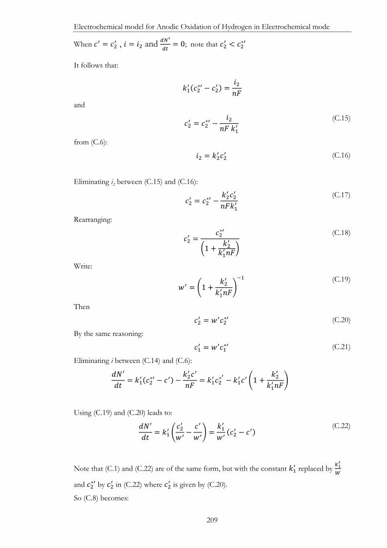
Electrochemical model for Anodic Oxidation of Hydrogen in Electrochemical mode
209
When 𝑐′ = 𝑐2′ , 𝑖 = 𝑖2 and
𝑑𝑁′
𝑑𝑡= 0; note that 𝑐2
′ < 𝑐2∗′
It follows that:
𝑘1′ (𝑐2
∗′ − 𝑐2′ ) =
𝑖2𝑛𝐹
and
𝑐2′ = 𝑐2
∗′ −𝑖2
𝑛𝐹 𝑘1′
(C.15)
from (C.6):
𝑖2 = 𝑘2′ 𝑐2′ (C.16)
Eliminating i2 between (C.15) and (C.16):
𝑐2′ = 𝑐2
∗′ −𝑘2′ 𝑐2′
𝑛𝐹𝑘1′
(C.17)
Rearranging:
𝑐2′ =
𝑐2∗′
(1 +𝑘2′
𝑘1′𝑛𝐹
)
(C.18)
Write:
𝑤′ = (1 +
𝑘2′
𝑘1′𝑛𝐹
)
−1
(C.19)
Then
𝑐2′ = 𝑤′𝑐2
∗′ (C.20)
By the same reasoning:
𝑐1′ = 𝑤′𝑐1
∗′ (C.21)
Eliminating i between (C.14) and (C.6):
𝑑𝑁′
𝑑𝑡= 𝑘1
′ (𝑐2∗′ − 𝑐′) −
𝑘2′ 𝑐′
𝑛𝐹= 𝑘1
′𝑐2∗′ − 𝑘1
′𝑐′ (1 +𝑘2′
𝑘1′𝑛𝐹
)
Using (C.19) and (C.20) leads to:
𝑑𝑁′
𝑑𝑡= 𝑘1
′ (𝑐2′
𝑤′−𝑐′
𝑤′) =
𝑘1′
𝑤′(𝑐2′ − 𝑐′)
(C.22)
Note that (C.1) and (C.22) are of the same form, but with the constant 𝑘1′ replaced by
𝑘1′
𝑊
and 𝑐2∗′ by 𝑐2
′ in (C.22) where 𝑐2′ is given by (C.20).
So (C.8) becomes:

Electrochemical model for Anodic Oxidation of Hydrogen in Electrochemical mode
210
𝑑𝑐′
𝑑𝑡=
1
𝑉𝑤′𝑘1′ (𝑐2
′ − 𝑐′) (C.23)
Integrating:
∫
𝑑𝑐′
(𝑐2′ − 𝑐′)
=𝑐′
𝑐1′
𝑘1′
𝑉𝑤′∫ 𝑑𝑡𝑡
𝑡1
− 𝑙𝑛
(𝑐2′ − 𝑐′)
(𝑐2′ − 𝑐1
′)=𝑘1′
𝑉𝑤′(𝑡 − 𝑡1)
(C.24)
From (C.6) it follows that:
− 𝑙𝑛
(𝑖2 − 𝑖)
(𝑖2 − 𝑖1)=𝑘1′
𝑉𝑤′(𝑡 − 𝑡1)
(C.25)
(Compare equation (C.10))
Predictions from Model 2:
These are as for Model 1, except that prediction ii) is modified to iia) as follows:
iia) A plot of 𝑙𝑛𝑖2−𝑖
𝑖2−𝑖1 versus t should show a straight line of slope -
𝑘1′
𝑉𝑤′ through
the origin (according to equation (C.25)).
Note that 𝑉𝑤′
𝑘1′ is the time constant for the curve of i versus t when a step-change is made in
hydrogen partial pressure.
Additional Mechanistic Theory A further case is now considered where an inert gas, Ar, is first bubbled through the tin for
sufficient time to reduce the hydrogen concentration to a value close to zero. The potential
of tin is held at constant value E at which residual hydrogen, if present, undergoes anodic
oxidation to water. Then, while holding the potential at this value, gas mixture of Ar/H2
with hydrogen partial pressure p2’ is bubbled continuously, starting at time t equal to zero
through the tin and the anodic current measured as a function of time.
At t =0, c’=0 and thus i=0 (Equation (C.6) with c’=0) Equation (C.14) becomes
[𝑑𝑁′
𝑑𝑡]𝑡=0
= 𝑘1′𝑐2∗′
(C.26)
As hydrogen is supplied to the tin the concentration of hydrogen begins to increase from
zero and it follows from (C.6) that

Electrochemical model for Anodic Oxidation of Hydrogen in Electrochemical mode
211
𝑑𝑖
𝑑𝑡= 𝑘2
′𝑑𝑐′
𝑑𝑡
(C.27)
and
𝑑𝑐′
𝑑𝑡=1
𝑉
𝑑𝑁′
𝑑𝑡
(C.7)
Combining (C.26), (C.27) and (C.7)
[𝑑𝑖
𝑑𝑡]𝑡=0
=𝑘1′𝑘2′ 𝑐2∗′
𝑉
(C.28)
Also from (C.12)
𝑐2∗′ = 𝑘3
′𝑝2′ (C.29)
Eliminating c2*’ between (C.28) and (C.29)
[𝑑𝑖
𝑑𝑡]𝑡=0
=𝑘1′𝑘2′𝑘3′
𝑉𝑝2′
(C.30)
Equation (C.30) predicts that [𝑑𝑖
𝑑𝑡]𝑡=0
should be proportional to p2’; a plot of [
𝑑𝑖
𝑑𝑡]𝑡=0
vs.
p2’is expected to reveal a slope of
𝑘1′𝑘2′𝑘3′
𝑉.
It has also been shown above that
𝑖2 = 𝑘2′ 𝑐2′ (C.16)
𝑐2′ = 𝑤′𝑐2
∗′ (C.20)
Combining these equations with (C.29):
𝑖2 = 𝑘2′𝑘3′𝑤′𝑝2
′ (C.31)
Equation (C.31) predicts a straight line though the origin with slope 𝑘2′𝑘3′𝑤′ for a plot of i2
vs. p2’. The ratio of the slopes of the above two plots using Equations (C.30) and (C.31)
provides a value of 𝑘1′
𝑉𝑤′ (see Equation (C.25)). So it should be possible to compare values
of k1’/Vw’ determined by two different methods.
Determination of the apparent solubility of H2 in
liquid tin and the parameter w’ using anodic
stripping voltammetry The development of the theoretical framework in the previous section has generated the
parameter w’. This parameter expresses the balance between addition of hydrogen to the tin

Electrochemical model for Anodic Oxidation of Hydrogen in Electrochemical mode
212
via dissolution and the removal of hydrogen from the tin via anodic oxidation to water.
Theory shown above postulates that w’ depends upon geometric factors, applied potential
and diffusion layer thickness (and hence degree of convection). Though not fundamental it
is important to determine its value in order to obtain an understanding of experimentally-
generated results. In broader sense this parameter will be important for the design of
systems consisting of two processes: physical dissolution of the gas in the melt and
electrochemical oxidation or reduction of the active gas via the liquid anode.
For the determination of w’ parameter as well as hydrogen solubility three regimes
of operation of LMA SOFC were proposed. The theory has been worked out for each of
the regimes, which is used together with experimental data for the calculation of w’ in
different cells and apparent solubility of H2 in liquid tin.
Regime 1
Consider the following operation where there are four stages (see Figure C.1 ). Prior to A,
argon is bubbled through liquid tin for a sufficient time to reduce the concentration of
hydrogen to a value close to zero and the tin electrode is held at an anodic potential E,
typically -0.90 V vs. RE (air electrode); the current at A is close to zero. During the
intervals A - B, B - C and C - D, hydrogen at partial pressure p’2 is bubbled through the tin.
The interval A - B is sufficiently long to allow the current to reach a steady value i2. During
the interval B - C, of length t3-t2, the tin electrode is switched to open circuit (OC). Then
during the interval C - D, the potential of the tin electrode is held at anodic potential E,
during which time the current is monitored. The period C - D is sufficiently long to allow
the current to return to the steady current i2.
Figure C.1 Schematic of Regime 1 conditions applied to the working cell (E mode). Same hydrogen partial pressure, p’
2 is applied from A to D. Potential is held at a value E everywhere except in B - C.
From the E model steady concentration of hydrogen in the bulk is c2’ at time t2:
𝑐2′ = 𝑤′𝑐2
∗′ (C.20)
A B
CD
O C

Electrochemical model for Anodic Oxidation of Hydrogen in Electrochemical mode
213
From B to C (at open circuit) i=0, so the equation that expressed the rate of dissolution of
hydrogen to the tin via and the removal of hydrogen from the tin via anodic oxidation to
water was shown above:
𝑑𝑁′
𝑑𝑡= 𝑘1
′ (𝑐2∗′ − 𝑐′) −
𝑖
𝑛𝐹
(C.14)
when treated from B - C Equation (C.14)becomes:
𝑑𝑁′
𝑑𝑡= 𝑘1
′ (𝑐2∗′ − 𝑐′)
(C.32)
From previous model:
𝑑𝑐′
𝑑𝑡=1
𝑉
𝑑𝑁′
𝑑𝑡
(C.7)
Using (C.32) and (C.7):
𝑑𝑐′
𝑑𝑡=1
𝑉𝑘1′ (𝑐2
∗′ − 𝑐′) (C.33)
Integrating (C.33)
−[𝑙𝑛 (𝑐2
∗′ − 𝑐′)]𝑐2′𝑐3′
=𝑘1′
𝑉[𝑡]𝑡2𝑡3
− 𝑙𝑛
𝑐2∗′ − 𝑐3
′
𝑐2∗′ − 𝑐2
′=𝑘1′
𝑉(𝑡3 − 𝑡2)
(C.34)
This becomes using (C.34) and (C.20):
− 𝑙𝑛
𝑐2∗′ − 𝑐3
′
𝑐2∗′(1 − 𝑤′)
=𝑘1′
𝑉(𝑡3 − 𝑡2)
(C.35)
−𝑙𝑛
1 −𝑐3′
𝑐2∗′⁄
(1 − 𝑤′)=𝑘1′
𝑉(𝑡3 − 𝑡2)
1 −𝑐3′
𝑐2∗′⁄
(1 − 𝑤′)= 𝑒𝑥𝑝 −
𝑘1′
𝑉(𝑡3 − 𝑡2)
1 −
𝑐3′
𝑐2∗′ = (1 − 𝑤
′)𝑒𝑥𝑝 −𝑘1′
𝑉(𝑡3 − 𝑡2)
𝑐3
′
𝑐2∗′ = 1 − (1 − 𝑤
′)𝑒𝑥𝑝 −𝑘1′
𝑉(𝑡3 − 𝑡2)

Electrochemical model for Anodic Oxidation of Hydrogen in Electrochemical mode
214
𝑐3′ = 𝑐2
∗′ [1 − (1 − 𝑤′)𝑒𝑥𝑝 −𝑘1′
𝑉(𝑡3 − 𝑡2)]
(C.36)
Using Equation (C.20):
𝑐3′ − 𝑐2
′ = 𝑐2∗′ [1 − (1 − 𝑤′)𝑒𝑥𝑝 −
𝑘1′
𝑉(𝑡3 − 𝑡2) − 𝑤
′]
𝑐3′ − 𝑐2
′ = 𝑐2∗′(1 − 𝑤′) [1 − 𝑒𝑥𝑝 −
𝑘1′
𝑉(𝑡3 − 𝑡2)]
(C.37)
Note that (t3 – t2) may be varied over a wide range.
The region from C-D is now treated. In this region, Equation (C.14)applies, i.e.:
𝑑𝑁′
𝑑𝑡= 𝑘1
′ (𝑐2∗′ − 𝑐′) −
𝑖
𝑛𝐹 (C.14)
Furthermore invoking Equation (C.25):
− 𝑙𝑛
(𝑐2′ − 𝑐′)
(𝑐2′ − 𝑐1
′)=𝑘1′
𝑉𝑤′(𝑡 − 𝑡1)
(C.25)
and replacing 𝑐′ by 𝑐3′ and 𝑡1by 𝑡3:
𝑙𝑛(𝑐′ − 𝑐2
′ )
(𝑐3′ − 𝑐2
′ )= −
𝑘1′
𝑉𝑤′(𝑡 − 𝑡3)
(C.38)
Where from (C.37) and (C.20):
𝑐3′ − 𝑐2
′ =𝑐2′
𝑤′(1 − 𝑤′) [1 − 𝑒𝑥𝑝 −
𝑘1′
𝑉(𝑡3 − 𝑡2)]
(C.39)
Substituting for 𝑐3′ − 𝑐2
′ from (C.39) into (C.38) and invoking Equation (C.6) which was
derived previously as follows:
𝑖 = 𝑘2′ 𝑐′ (C.6)
Obtain:
𝑙𝑛
𝑖 − 𝑖2
𝑖2 (1 − 𝑤′
𝑤′ ) [1 − 𝑒𝑥𝑝 −𝑘1′
𝑉(𝑡3 − 𝑡2)]
= −𝑘1′
𝑉𝑤′(𝑡 − 𝑡3)
(C.40)
So
𝑖 − 𝑖2 = 𝑖2 (
1 − 𝑤′
𝑤′) [1 − 𝑒𝑥𝑝 −
𝑘1′
𝑉(𝑡3 − 𝑡2)] 𝑒𝑥𝑝 −
𝑘1′
𝑉𝑤′(𝑡 − 𝑡3)
(C.41)
The charge shown by the shaded area in the diagram is given by:
𝑄′1 = ∫ (𝑖 − 𝑖2)𝑑𝑡 = 𝑖2
1 − 𝑤′
𝑤′
∞
0
[1 − 𝑒𝑥𝑝 −𝑘1′
𝑉(𝑡3 − 𝑡2)]
×∫ 𝑒𝑥𝑝 −𝑘1′
𝑉𝑤′(𝑡 − 𝑡3) 𝑑𝑡
∞
𝑡3
(C.42)
Or
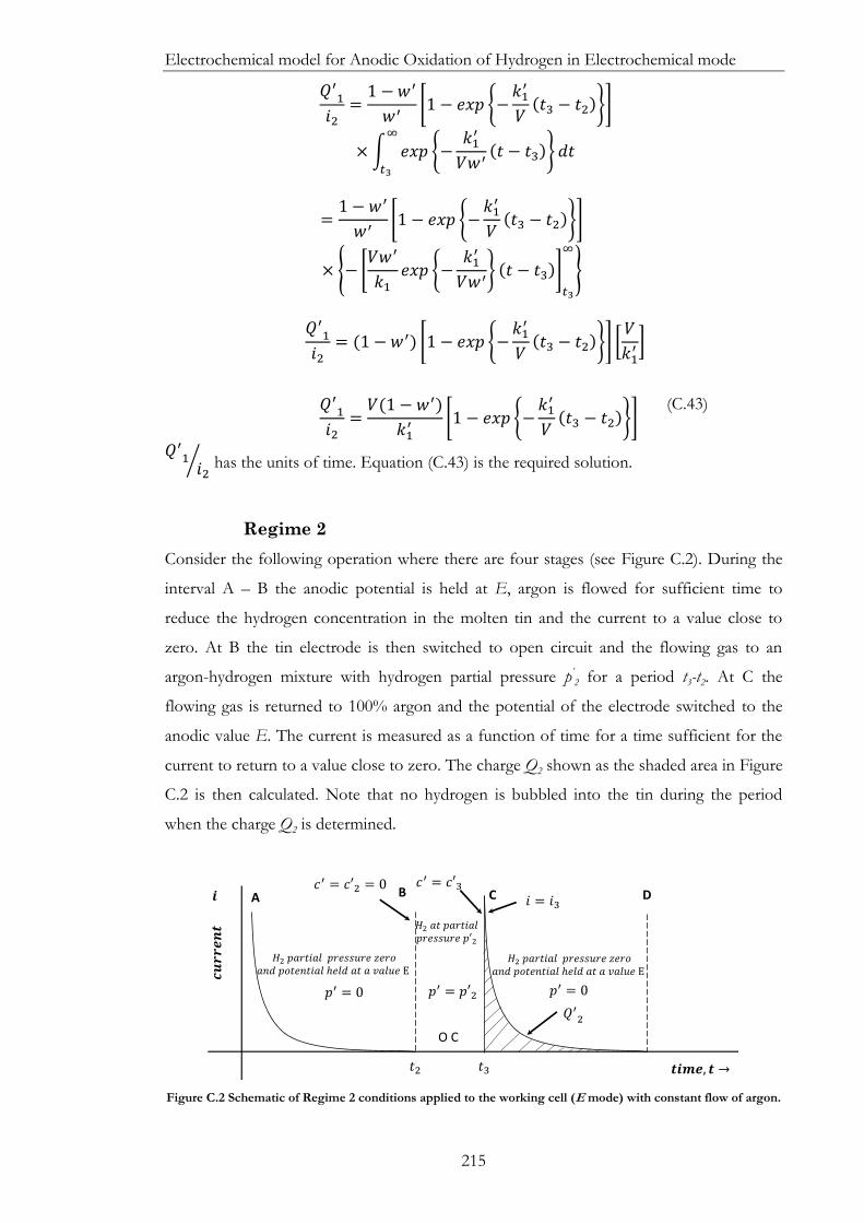
Electrochemical model for Anodic Oxidation of Hydrogen in Electrochemical mode
215
𝑄′1𝑖2=1 −𝑤′
𝑤′[1 − 𝑒𝑥𝑝 −
𝑘1′
𝑉(𝑡3 − 𝑡2)]
×∫ 𝑒𝑥𝑝 −𝑘1′
𝑉𝑤′(𝑡 − 𝑡3) 𝑑𝑡
∞
𝑡3
=1 − 𝑤′
𝑤′[1 − 𝑒𝑥𝑝 −
𝑘1′
𝑉(𝑡3 − 𝑡2)]
× − [𝑉𝑤′
𝑘1𝑒𝑥𝑝 −
𝑘1′
𝑉𝑤′ (𝑡 − 𝑡3)]
𝑡3
∞
𝑄′1
𝑖2= (1 − 𝑤′) [1 − 𝑒𝑥𝑝 −
𝑘1′
𝑉(𝑡3 − 𝑡2)] [
𝑉
𝑘1′ ]
𝑄′1𝑖2=𝑉(1 − 𝑤′)
𝑘1′ [1 − 𝑒𝑥𝑝 −
𝑘1′
𝑉(𝑡3 − 𝑡2)]
(C.43)
𝑄′1𝑖2⁄ has the units of time. Equation (C.43) is the required solution.
Regime 2
Consider the following operation where there are four stages (see Figure C.2). During the
interval A – B the anodic potential is held at E, argon is flowed for sufficient time to
reduce the hydrogen concentration in the molten tin and the current to a value close to
zero. At B the tin electrode is then switched to open circuit and the flowing gas to an
argon-hydrogen mixture with hydrogen partial pressure p’2 for a period t3-t2. At C the
flowing gas is returned to 100% argon and the potential of the electrode switched to the
anodic value E. The current is measured as a function of time for a time sufficient for the
current to return to a value close to zero. The charge Q2 shown as the shaded area in Figure
C.2 is then calculated. Note that no hydrogen is bubbled into the tin during the period
when the charge Q2 is determined.
Figure C.2 Schematic of Regime 2 conditions applied to the working cell (E mode) with constant flow of argon.
A B C D
O C

Electrochemical model for Anodic Oxidation of Hydrogen in Electrochemical mode
216
For the interval B – C Equation (C.32) pertains:
𝑑𝑁′
𝑑𝑡= 𝑘1
′ (𝑐2∗′ − 𝑐′)
(C.32)
and
𝑑𝑐′
𝑑𝑡=𝑘1′
𝑉(𝑐2∗′ − 𝑐′)
(C.33)
Integrating (C.33):
−[𝑙𝑛(𝑐2
∗′ − 𝑐′)]0
𝑐3′
=𝑘1′
𝑉[𝑡]𝑡2
𝑡3
−𝑙𝑛𝑐2∗′ − 𝑐3
′
𝑐2∗′
=𝑘1′
𝑉(𝑡3 − 𝑡2)
(C.44)
Compare with (C.34)
−𝑙𝑛 (1− 𝑐3
′
𝑐2∗′) =
𝑘1′
𝑉(𝑡3 − 𝑡2)
𝑐3′
𝑐2∗′= 1 − 𝑒𝑥𝑝 [−
𝑘1′
𝑉(𝑡3 − 𝑡2)]
𝑐3′ = 𝑐2
∗′ [1 − 𝑒𝑥𝑝 −𝑘1′
𝑉(𝑡3 − 𝑡2)]
(C.45)
Compare (C.45) with (C.37). Note that w’ does not appear in (C.45).
We now treat region C – D. Equation (C.14)is modified to
𝑑𝑁′
𝑑𝑡= 𝑘1
′ (0 − 𝑐′) −𝑖
𝑛𝐹
(C.46)
The zero in (C.46) reflects the fact that the gas composition contains no hydrogen in this
region.
Eliminating i between (C.46) and (C.6):
𝑑𝑁′
𝑑𝑡= −𝑘1
′𝑐′ −𝑘2′ 𝑐′
𝑛𝐹
= −𝑐′ (𝑘1′ +
𝑘2′
𝑛𝐹)
= −𝑘1′𝑐′ (1 +
𝑘2′
𝑘1′𝑛𝐹
)
= −𝑘1′𝑐′
𝑤′
Using Equation (C.7) becomes:

Electrochemical model for Anodic Oxidation of Hydrogen in Electrochemical mode
217
𝑑𝑐′
𝑑𝑡= −
𝑘1′𝑐′
𝑉𝑤′
(C.47)
Compare it with (C.33)
Integrating (C.47):
∫
𝑑𝑐′
𝑐′= −∫
𝑘1′
𝑉𝑤′𝑑𝑡
𝑡
𝑡3
𝑐′
𝑐3′
[𝑙𝑛 𝑐′]𝑐3′𝑐′ = [−
𝑘1′ 𝑡
𝑉𝑤′]𝑡3
𝑡
𝑙𝑛𝑐′
𝑐3′ = −
𝑘1′
𝑉𝑤′(𝑡 − 𝑡3)
(C.48)
Using (C.6):
𝑙𝑛𝑖
𝑖3= −
𝑘1′
𝑉𝑤′(𝑡 − 𝑡3)
(C.49)
Or
𝑖 = 𝑖3𝑒𝑥𝑝 −𝑘1′
𝑉𝑤′(𝑡 − 𝑡3)
(C.50)
The charge, Q’2, shown in the diagram is given by
𝑄′2 = ∫ 𝑖𝑑𝑡
∞
𝑡3
= ∫ 𝑖3𝑒𝑥𝑝 −𝑘1′
𝑉𝑤′(𝑡 − 𝑡3) 𝑑𝑡
∞
𝑡3
𝑄′2 =−𝑉𝑤′𝑖3𝑘1′ [𝑒𝑥𝑝 −
𝑘1′
𝑉𝑤′(𝑡 − 𝑡3)]
𝑡3
𝑡
=𝑉𝑤′𝑖3𝑘1′
(C.51)
Writing 𝑐2∗′ = 𝑐2
′/𝑤′ equation (C.45) becomes:
𝑐3′ =
𝑐2′
𝑤′[1 − 𝑒𝑥𝑝 −
𝑘1′
𝑉(𝑡3 − 𝑡2)]
(C.52)
Applying (C.6), Equation (C.52) becomes:
𝑖3 =
𝑖2𝑤′[1 − 𝑒𝑥𝑝 −
𝑘1′
𝑉(𝑡3 − 𝑡2)]
(C.53)
Substituting for i3 in (C.51)
𝑄′2𝑖2=𝑉
𝑘1′ [1 − 𝑒𝑥𝑝 −
𝑘1′
𝑉(𝑡3 − 𝑡2)]
(C.54)
Compare (C.54) with (C.43)
Regime 3
This case is included for completeness. However no experiments are performed to support
theory developed in this section (for Regime 3). Figure C.3 describes the regime which is a
combination of the previous two regimes.

Electrochemical model for Anodic Oxidation of Hydrogen in Electrochemical mode
218
Figure C.3 Schematic of Regime 3 conditions applied to the working cell (E mode) with constant flow of argon. Potential is held at a value E everywhere except in B-C.
Prior to A argon is bubbled through tin for a sufficient time to reduce the concentration of
hydrogen to a value close to zero and the tin electrode is held at an anodic potential E,
typically -0.90 V, with respect to an air electrode; the current at A is close to zero. During
the intervals A - B, B - C , hydrogen at partial pressure p2 is bubbled through the tin. The
interval A - B is sufficiently long to allow the current to reach a steady value i2. During the
interval B - C, of length t3-t2, the tin electrode is switched to open circuit. At C the flowing
gas is returned to 100% argon and the potential of the electrode switched to the anodic
value E. The current is measured as a function of time for a time sufficient for the current
to return to a value close to zero. The charge Q3 shown as the shaded area in Figure C.3 is
then calculated. Note that no hydrogen is bubbled into the tin during the period when the
charge Q3 is determined.
Following Regime 1 we have the hydrogen concentration c’3 at C given by (C.36):
𝑐3′ = 𝑐2
∗′ [1 − (1 − 𝑤′)𝑒𝑥𝑝 −𝑘1′
𝑉(𝑡3 − 𝑡2)]
(C.36)
For the Region C – D Equation (C.51) applies and leads to
𝑄3 =
𝑉𝑤′𝑖3
𝑘1′
(C.55)
The next equation ((C.17)) has been derived previously:
𝑐2′ = 𝑐2
∗′ −𝑘2′ 𝑐2′
𝑛𝐹𝑘1′
Using(C.36), (C.6) and (C.20):
𝑖3 =
𝑖2𝑤′[1 − (1 − 𝑤′)𝑒𝑥𝑝 −
𝑘1′
𝑉(𝑡3 − 𝑡2)]
(C.56)
(Compare it to Equation (C.53))
Note that i3 in (C.51) ≠i3 in (C.55). Substituting for i3 from (C.56) into (C.55):
A B
C D
O C

Electrochemical model for Anodic Oxidation of Hydrogen in Electrochemical mode
219
𝑄′3 =
𝑉𝑖2
𝑘1′[1 − (1 − 𝑤′)𝑒𝑥𝑝 −
𝑘1′
𝑉(𝑡3 − 𝑡2)]
Or 𝑄′3
𝑖2=𝑉(1 − 𝑤′)
𝑘1′
[1 − 𝑒𝑥𝑝 −𝑘1′
𝑉(𝑡3 − 𝑡2)] +
𝑤′𝑉
𝑘1′
(C.57)
Comparing (C.57) and (C.43) it is noted that they are identical apart from the additional
term 𝑤′𝑉
𝑘1′ in (C.57).
The important equations in the above sections are those that allow interpretation of the
coulombic charge under the final parts of the regimes, i.e. C – D. These are as follows:
Regime 1 𝑄′1𝑖2=𝑉(1 − 𝑤′)
𝑘1′ [1 − 𝑒𝑥𝑝 −
𝑘1′
𝑉(𝑡3 − 𝑡2)]
(C.43)
Regime 2 𝑄′2𝑖2=𝑉
𝑘1′ [1 − 𝑒𝑥𝑝 −
𝑘1′
𝑉(𝑡3 − 𝑡2)]
(C.54)
Regime 3 𝑄′3𝑖2=𝑉(1 − 𝑤′)
𝑘1′
[1 − 𝑒𝑥𝑝 −𝑘1′
𝑉(𝑡3 − 𝑡2)] +
𝑤′𝑉
𝑘1′
(C.57)
Determination of the parameter w’
The development of this theoretical framework has generated the parameter w’. This
parameter expresses the balance between addition of hydrogen to the tin via dissolution
and the removal of hydrogen from the tin via anodic oxidation to water.
For a given value of (t3 – t2) and the same p’2 value (and i2 value) (C.43) and (C.54) show
that:
𝑤′ = 1 −
𝑄′1𝑄′2
(C.58)
The given value of (t3 – t2) may be then varied and the w’ value determined for each case.
The w’ value would be expected to be independent of (t3 – t2).