Mechanisms of Thermohaline Mode Switching with Application ...paoc.mit.edu/paoc/papers/mode_switch.pdf · Mechanisms of Thermohaline Mode Switching with Application to ... It is found

2056 VOLUME 15J O U R N A L O F C L I M A T E

q 2002 American Meteorological Society

Mechanisms of Thermohaline Mode Switching with Application toWarm Equable Climates

RONG ZHANG,* MICHAEL FOLLOWS, AND JOHN MARSHALL

Department of Earth, Atmospheric and Planetary Sciences, Massachusetts Institute of Technology, Cambridge, Massachusetts

(Manuscript received 10 August 2001, in final form 12 December 2001)

ABSTRACT

A three-box model of haline and thermal mode overturning is developed to study thermohaline oscillationsfound in a number of ocean general circulation models and that might have occurred in warm equable paleo-climates. By including convective adjustment modified to represent the localized nature of deep convection, thebox model shows that a steady haline mode circulation is unstable. For certain ranges of freshwater forcing/vertical diffusivity, a self-sustained oscillatory circulation is found in which haline–thermal mode switchingoccurs with a period of centuries to millennia. It is found that mode switching is most likely to occur in warmperiods of earth’s history with, relative to the present climate, a reduced Pole–equator temperature gradient, anenhanced hydrological cycle, and somewhat smaller values of oceanic diffusivities.

1. Introduction

In past climates the thermohaline circulation (THC)of the ocean may have been quite different from that oftoday. Paleoclimatic records (e.g., Railsback et al. 1990)suggest that in warm periods of earth’s history the abys-sal ocean was very much warmer than that of today. Arecurring theme of the paleoclimatic literature is thespeculation that in these warm climates ocean deep wa-ter formation could have been triggered by evaporationfrom the subtropics resulting in a ‘‘haline mode’’ ac-counting for abnormal warmth in the subsurface ocean(e.g., Brass et al. 1982). This is very different fromtoday’s climate in which deep water formation at highlatitudes brings cold water to depth in a ‘‘thermalmode.’’ Such extremes of ocean circulations have verydifferent implications for climate and biogeochemicalcycles [see, e.g., Zhang et al. (2001)].

In certain parameter regimes, ocean general circula-tion models (OGCMs) exhibit ‘‘mode switching’’ inwhich the meridional overturning circulation (MOC)switches between thermal and haline modes. Self-sus-tained thermohaline oscillations have been found in sev-eral OGCM studies using an idealized single basin con-figuration (Marotzke 1989; Wright and Stocker 1991;

* Current affiliation: Geophysical Fluid Dynamics Laboratory,Princeton University, Princeton, New Jersey

Corresponding author address: Dr. Rong Zhang, Geophysical Flu-id Dynamics Laboratory, P.O. Box 308, Princeton University, Prince-ton, NJ 08542E-mail: [email protected]

Weaver and Sarachik 1991a,b; Weaver et al. 1993; Win-ton and Sarachik 1993; Huang 1994). In a study ofpossible modes of the late Permian ocean circulationwith a coarse-resolution OGCM (Zhang et al. 2001), wefound that the haline mode (HM) was inherently unsta-ble for fixed external forcing, periodically switching into a transient thermal mode (TM) in which deep waterformed in polar regions (‘‘flushing events’’; Marotzke1989), and gradually returning to the HM to close thelimit cycle. Such internal thermohaline oscillationsmight have significant implications for understandingthe paleoclimatic record, such as the centuries to mil-lennia oscillations during glacial periods (Johnson et al.1992). Such oscillations do not appear to occur in themodern ocean, because, apparently, the surface fresh-water forcing is not strong enough. Mode switching ismore likely to occur, perhaps, during glacial periods inwhich the freshwater forcing due to ice melting at polarregions is much stronger, or during warm equable pa-leoclimates such as the late Permian, or mid-Cretaceousin which the buoyancy forcing due to freshwater fluxmay have been stronger than the air–sea heat flux.

The physical mechanism underlying such thermo-haline oscillations has yet to be clearly articulated.Stommel (1961) first showed, using a highly idealizedbox model, that the THC can have multiple steady stateswhen the freshwater forcing is strong enough: he founda strong stable TM circulation, a weak unstable TMcirculation, and a stable HM circulation. Since Stom-mel’s (1961) pioneering work, many box models havebeen constructed to study the multiple steady solutionsof the THC (e.g., Rooth 1982; Huang et al. 1992). With-out convective adjustment, Stommel-type box models

1 AUGUST 2002 2057Z H A N G E T A L .

cannot support self-sustained oscillations (Ruddick andZhang 1996). Welander (1982) proposed a heat–salt os-cillator using a model with convective adjustment be-tween the surface and deep ocean whose temperatureand salinity were fixed. It exhibits self-sustained oscil-lations only when warm salty water convects over coldfreshwater. This kind of convection is likely to happenin low latitudes, but not in polar regions. Winton (1993)modified this model by fixing the surface temperaturebut allowing deep ocean temperature to vary. He ob-tained a self-sustained oscillation with polar convectionwhen a nonlinear equation of state for seawater wasused. Pierce et al. (1995) also obtained a self-sustainedoscillation by modifying Welander’s convection modelto allow both surface and deep ocean temperatures andsalinity to vary, and again using a nonlinear equationof state for density.

In this study, we construct a simple box model withconvective adjustment and assume a linear equation ofstate. It combines the Stommel-type box model with theWelander-type convection model. The model capturesthe main character and essential physics of the ther-mohaline oscillation and instability exhibited in ourmodel of the late Permian ocean circulation. When com-bined with our OGCM studies we are able to explainwhy the steady HM becomes unstable in a certain rangeof freshwater forcing and vertical diffusivity amplitude.We then go on to use the box model as an economicaltool to explore parameter space, identify regimes andtheir stability, and the dependence of oscillation periodto freshwater flux forcing and vertical diffusivity.

In section 2, we describe in detail the millennial ther-mohaline oscillation in a global OGCM configured withlate Permian bathymetry. In section 3, we discuss themechanism of such oscillations using a simple three-box model.

2. Self-sustained thermohaline oscillation in anOGCM of late Permian ocean

We briefly review thermohaline mode switching ob-served in certain parameter regimes of a global, coarse-resolution OGCM (Marshall et al. 1997a,b) configuredfor late Permian bathymetry (Fig. 1a; see appendix A;Zhang et al. 2001). The late Permian (about 250 millionyears ago) is thought to have been a period of warmequable climate (Taylor et al. 1992). In our model aquasi-steady HM circulation occurred with enhanced(relative to the modern) freshwater flux forcing [a max-imum evaporation 2 precipitation (E 2 P) of 1.3 myr21 compared to 0.6 m yr21 in the present climate] anda relatively weak background vertical mixing in theocean of magnitude M 5 3 3 1025 m2 s21. This shouldbe compared to the canonical, global average value ofabout 5 3 1025 m2 s21, required to bring into consis-tency deep water formation rates and the mean tem-perature structure of the modern ocean in OGCMs. Inreality, oceanic diapycnal mixing is thought to be spa-

tially inhomogeneous becoming larger near boundarieswhere tidally induced mixing processes may dominate(Toole et al. 1994; Marotzke 1997; Munk and Wunsch1998).

Figure 1b shows the meridional overturning circu-lation of the model during the quasi-steady HM. Asdescribed in appendix A, mixed boundary conditionsand a full nonlinear equation of state are used. Theoverturning is weak and shallow; warm, salty inter-mediate water is formed in the subtropics, then returnsto the surface in polar regions and the Tropics. Figure1c illustrates the meridional overturning circulation dur-ing a transient TM (a ‘‘flushing’’ event), which is strongand deep; deep water formed in the southern polar re-gion upwells in the Tropics and Northern Hemisphere.Here the transient TM circulation shows strong hemi-spheric asymmetry, that is, a relative warm SST insouthern high latitudes is associated with strong deepconvection there and coexists with a relatively cool SSTin the northern high latitudes where deep convection isabsent. This result is very similar to the recent study byHaupt and Seidov (2001), in which for asymmetric sur-face thermal forcing, a strong asymmetric ocean cir-culation can sustain a warm abyss through deep con-vection while keeping the other Pole cool. Since herewe have symmetric surface forcing, the asymmetric cir-culation obtained is a consequence of the asymmetricdistribution of land and sea. Both studies show that thethermal mode overturning circulation is sensitive to thehigh-latitude freshwater flux and that a symmetric cir-culation with deep convection in both hemispheres isdifficult to sustain.

The onset of the flushing event is triggered by intenselocal convection in the southern polar region, inducedby meridional transports of warm salty surface water bya large eddy. Figure 2 shows the sea surface temperature(SST) and salinity at year 4155, just before the switchfrom HM to transient TM. A large-scale eddy, warmerand saltier than the ambient polar surface water, isformed near the western boundary of the superocean inthe southern polar region, just where strong local con-vection occurs. The eddy propagates toward the easternboundary of the superocean at the latitude of strong deepconvection in the TM and, we believe, plays a role inflipping the circulation into a strong transient TM. Whenthe convection region becomes less dense due to pre-cipitation, convection ceases and the circulation returnsto the HM.

The transient TM is asymmetric, with deep convec-tion occurring at southern high latitudes. Hence, wefocus our diagnostics on the southern ocean of the mod-el. We divide the southern ocean into three distinct re-gions over which we consider time series of averageproperties. These regions are low-latitude surface (148–36.68S, 0–50 m), high-latitude surface (36.68–70.38S,0–50 m), and deep ocean (148–70.38S, 50–4000 m). Insection 3 we will describe a simple three-box model


FIG. 1. OGCM studies of the late Permian: (a) late Permian bathymetry (ocean depth in km), (b) overturning streamfunction of HM atyear 3975, (c) overturning streamfunction of the transient TM at year 4275. Contour interval is in Sverdrups (Sv; where 1Sv [ 106 m3 s21),positive contour means counterclockwise flow, negative contour means clockwise flow.

inspired by the diagnosis of these three regions in theOGCM.

Figure 3 shows the time series of mean temperatureTi, and salinity Si[i 5 l, h, d; l, low-latitude surface; h,high-latitude surface; d, deep ocean; and the caret () isa dimensional quantity] in the OGCM over a period of8000 yr. The period of oscillation is about 3300 yr andtwo cycles are captured. Note that Td increases duringthe persistent, quasi-steady HM; Td falls with the onsetof deep convection at high southern latitudes. The cycleis asymmetric; the quasi-steady HM lasts much longerthan the transient TM period.

Figure 4 shows the time series of the nondimensional(without a caret) vertical density difference between sur-face regions and deep ocean

r 2 r r 2 rl d h dDr 5 , Dr 5 ,ld hdˆ ˆr aDT r aDT0 A 0 A

based on a linear equation of state for density. Herei(i 5 l, h, d) is the density of each region, 0 is ther r

mean ocean density, DTA 5 TAl 2 TAh is the polar–equator surface air temperature difference, and a is thethermal expansion coefficient. During the unsteady HM,the mean trend of Drhd increases gradually (Fig. 4b),that is, d(Drhd)/dt . 0, until Drhd reaches the thresh-old—which we call «—for the onset of polar convec-tion, that is, Drhd 5 « ø 21.1. Then, suddenly, strongpolar convection begins, Drhd jumps to a very high val-ue, and the circulation switches to the transient TM.Polar convection begins even though the zonal meandensity structure is still statically stable (Drhd 5 « ,0), because, as discussed above, convection only occursin a localized, statically unstable region (Fig. 2). Thewarm, salty surface eddy (Fig. 2) is cooled quickly,locally destabilizing the water column. As the abyssaltemperature increases, the deep ocean density d de-rcreases until it becomes almost the same as the densityof the large-scale eddy eddy in the high-latitude surface.rThus when Drhd reaches «, convection occurs, and « ø( h 2 eddy)/( 0aDTA) , 0.r r r


FIG. 2. SST and salinity during the switch from the HM to the TM in our simulation of thelate Permian ocean circulation: (a) SST at year 4155 and (b) sea surface salinity (SSS) at year4155.

During the switch from HM to TM, the mean polarsurface temperature and salinity (Figs. 3c,d) increasesignificantly due to strong mixing and horizontal ad-vection from low to high latitudes. During the transientTM, the mean trend of Drhd (Fig. 4b) decreases grad-ually [d(Drhd)/dt , 0], because the deep ocean densityincreases due to polar convection. Finally, when thefreshwater forcing becomes dominant again, the densityof the surface convective region becomes less than thatof the deep ocean, that is, Drhd reaches the thresholdfor the termination of polar convection: Drhd 5 hh ø20.3 (Fig. 4b), convection ceases and Drhd drops sharp-ly.

3. Self-sustained thermohaline oscillation in asimple box model

a. Box model description

To better understand the mechanism of the thermo-haline switching reviewed in section 2, we developeda simple three-box model inspired by study of theOGCM results. For simplicity the three-box model onlyrepresents a single hemisphere and combines the Stom-

mel-type box model (Fig. 5a) with the Welander-typeconvection model (Fig. 5b). It includes a low-latitudesurface box (from latitude 128 to 358), a high-latitudesurface box (from latitude 358 to 708), and a deep oceanbox (Fig. 5c). The horizontal diffusivity between surfaceboxes is K, which represents lateral eddy mixing. Thevertical diffusivities between the surface and deep oceanin low and high latitudes are, respectively, Ml and Mh,and are functions of the vertical density difference.

Let Tl, Th, Td be the mean temperature of the low-latitude surface box, high-latitude surface box, and deepocean box, respectively; and let Sl, Sh, Sd be the meansalinity of the low-latitude surface box, high-latitudesurface box, and deep ocean box, respectively. At theair–sea surface, there is a net mean freshwater flux Finto the high-latitude box, transported from the low-latitude box. The sea surface temperature Tl, Th is re-stored to the air temperature TAl, TAh at rate constant l,of a form similar to the boundary conditions used inthe OGCM. Let h be the depth of the surface box; Hbe the depth of the deep ocean box; Vl, Vh, and Vd bethe volume of each box, (here, for the given latituderange of our chosen surface boxes, we have Vl 5 Vh 5


FIG. 3. Time series of mean temperature and salinity in each diagnosed region of the OGCM: (a) Td, (b)Sd, (c) Th, (d) Sh, (e) Tl, and (f ) Sl. The total salinity of the chosen regions is not conserved. To comparewith the three-box model (described in section 3) in which the total salinity is conserved, the mean salinityanomaly of the three regions is subtracted from the salinity of each region.

FIG. 4. Time series of mean surface and deep ocean nondimensionaldensity difference of the OGCM: (a) Drld and (b) Drhd.

V); and L be the horizontal distance between the centerof the surface boxes (Fig. 5c). Notice that F is the netmean freshwater flux in each box, so it is about half ofthe peak of the zonal mean latitude-dependent fresh-water flux E 2 P. For example, the modern zonal meanE 2 P profile that has a maximum of about 0.6 m yr21,corresponds to F ø 0.3 m yr21.

The overturning streamfunction q (unit: Sv [ 106 m3

s21) is assumed to be linearly proportional to the surfacedensity gradient, as in Stommel’s model

q 5 m (r 2 r ),q h l (1)where q . 0 indicates a TM circulation (polar sinking),q , 0 indicates an HM circulation (subtropical sinking),and mq is the constant of proportionality.

We use a linear equation of state for seawaterˆ ˆ ˆ ˆr 5 r [1 2 a(T 2 T ) 1 b(S 2 S )],i 0 i r i r (2)

where 0, Tr, Sr are the reference density, temperature,rand salinity; and a, b are the thermal and saline ex-pansion coefficients, respectively.

The dimensional dynamic equations for T, S in eachbox are based on an upstream differencing scheme. Forexample, the high-latitude surface temperature T h

evolves due to air–sea heat flux, advection by over-turning circulation, and mixing by horizontal diffusionand vertical diffusion.

For the TM (q . 0), we haveˆ ˆdT q Kh ˆ ˆ ˆ ˆ ˆ ˆ5 l(T 2 T ) 1 (T 2 T ) 1 (T 2 T )Ah h l h l h2dt V Lh

Mh ˆ ˆ1 (T 2 T ). (3)d hh 1 Hh

2For the HM (q , 0), we have


FIG. 5. (a) Schematic diagram of the Stommel-type box model. (b)Schematic diagram of Welander-type convection model. (c) Sche-matic diagram of the three-box model. The horizontal diffusivitybetween surface boxes is K; Ml, Mh are the vertical diffusivities be-tween surface and deep ocean in low and high latitude, respectively.Net mean freshwater flux F entering the high-latitude surface box isbalanced by outflux from the low-latitude surface box. The SST Tl,Th is restored to the air temperature TAl, TAh with restoration rate l.The overturning strength is q. The surface box has depth h; the deepbox has depth H.

ˆ ˆdT q Kh ˆ ˆ ˆ ˆ ˆ ˆ5 l(T 2 T ) 2 (T 2 T ) 1 (T 2 T )Ah h d h l h2dt V Lh

Mh ˆ ˆ1 (T 2 T ). (4)d hh 1 Hh

2

We can write the above two equations in a form suit-able for both the TM (q . 0) and HM (q , 0), thus,

ˆdT qh ˆ ˆ ˆ ˆ5 l(T 2 T ) 1 (T 2 T )Ah h l ddt 2Vh

ˆ|q | Kˆ ˆ ˆ ˆ ˆ1 (T 1 T 2 2T ) 1 (T 2 T )l d h l h22V Lh

Mh ˆ ˆ1 (T 2 T ). (5)d hh 1 Hh

2

The complete dimensional equations for T, S in eachbox are written out in detail in appendix B.

1) NONDIMENSIONAL EQUATIONS

To nondimensionalize, let DTA 5 TAl 2 TAh (polar–equator surface air temperature difference) and 5TA

(TAl 1 TAh)/2 (mean surface air temperature). The con-trolling nondimensional parameters can then be iden-tified as

ˆDTAg 5 (pole–equator air temperatureTA difference),

2Fc 5 (freshwater flux),

lh

ˆ2KK 5 (horizontal diffusivity),

2L l

MlM 5 (vertical diffusivity in low latitudes),l h 1 Hhl

2

MM 5 (vertical diffusivity in high latitudes),h h 1 H

hl2

andˆ ˆm r aT h bSq 0 A 0m 5 , d 5 , R 5 .f ˆlV H aDTA

The nondimensional dynamical variables areˆ ˆ ˆ ˆ ˆT 2 T T 1 T Tl h l h dDT 5 , T 5 , T 5 ,dˆ ˆ ˆDT 2T TA A A

ˆ ˆ ˆ ˆS 2 S S 1 S Sl h l h dDS 5 , S 5 , S 5 .dˆ ˆ ˆS 2S S0 0 0

The nondimensional overturning streamfunction is f 5q/(glV), and Eq. (1) becomes

f 5 m (DT 2 RDS).f (6)

Based on the dimensional equations written out infull in appendix B, we write the nondimensional equa-tions in terms of the nondimensional variables DT, ,TTd, DS, , Sd for both TM ( f . 0) and HM ( f , 0)Scirculation. They are (where t9 5 lt is nondimensionaltime)


dDT 35 1 2 DT 1 f (T 2 T ) 2 | f |gDT 2 KDTddt9 2

1 DT1 M (T 2 T ) 2l d[ ]g 2

1 DT2 M (T 2 T ) 1 , (7)h d[ ]g 2

2dT g g5 1 2 T 1 | f |(T 2 T ) 1 f DTddt9 2 4

M gDTl1 T 2 T 2d1 22 2

M gDTh1 T 2 T 1 , (8)d1 22 2

2dT g gd 5 2d | f |(T 2 T ) 1 f DTd[dt9 2 4

M gDTl1 T 2 T 2d1 22 2

M gDTh1 T 2 T 1 , (9)d1 2]2 2

dDS 35 c 1 f g(S 2 S ) 2 | f |gDS 2 KDSddt9 2

DS1 M S 2 S 2l d1 22

DS2 M S 2 S 1 , (10)h d1 22

dS g g5 | f |(S 2 S ) 1 f DSddt9 2 4

M DSl1 S 2 S 2d1 22 2

M DSh1 S 2 S 1 , (11)d1 22 2

dS dSd 5 2d . (12)dt9 dt9

We will examine both steady and time-dependent so-lutions of these equations, respectively.

2) REPRESENTATION OF CONVECTION

The nondimensional vertical diffusivities Ml, Mh inthe above equations depend on the ocean state due toconvective process. We make the values of Ml and Mh

functions of the nondimensional mean vertical densitydifference between the surface box and deep ocean box

Dri(i 5 ld, hd) as discussed in section 2. If no con-vection occurs at low or high latitudes, then Ml 5 Mor Mh 5 M, where M 5 2M/[(h 1 H)hl] is the non-dimensional background vertical diffusivity (M is thedimensional background vertical diffusivity). When thedensity difference is conducive to convection at low(high) latitude, Ml(Mh) becomes much larger than M.

Based on the diagnosis of the OGCM in section 2,we represent the effect of local polar convection in ourthree-box model by introducing a threshold, «, for theonset of polar convection. Here the physical meaningof « is the same as found in the OGCM (see section 2and Fig. 4b): during the unsteady HM [d(Drhd)/dt . 0],when the mean nondimensional density difference be-tween the polar surface and deep ocean reaches thisthreshold, that is, Drhd 5 «, polar convection starts. Ifit does not reach this threshold, that is, Drhd , «, polarconvection can never occur. Here « , 0 represents theeffect of localized polar convection discussed in section2. Similarly, when the system is in its polar convectionphase, we introduce a threshold, hh, for the terminationof polar convection (see section 2 and Fig. 4b): whenDrhd , hh during the transient TM [d(Drhd)/dt , 0],polar convection terminates. During the polar convec-tive phase, the high-latitude surface density is spatiallymore homogeneous than that in the nonconvectivephase, so hh . « and hh is set to be close to zero inthe box model.

To summarize, we can write the following simplifiedrules for convective adjustment that include the effectof local convection in the three-box model.

At high latitudes,

if Drhd , «, then Mh 5 M (no convection);if Drhd $ «, and d(Drhd)/dt . 0, then Mh 5 Msc (strong

convection);if Drhd $ «, and d(Drhd)/dt # 0, then

if Drhd , hh, then Mh 5 M (no convection);if Drhd $ hh, then Mh 5 Msc (strong convection).

Here Msc k M, indicating that vertical mixing of coldfresh surface water in high latitudes is strong and deep.

At low latitudes,

if Drld , hl, then Ml 5 M (no convection);if Drld $ hl, then Ml 5 Mwc (weak convection).

Here Msc . Mwc k M, indicating that vertical mixingof warm salty surface water in low latitudes is weakand shallow compared to strong, deep convection inhigh latitudes. Because the density distribution in lowlatitudes is horizontally more homogeneous than in highlatitudes, we use the same threshold, hl, close to zero,for the onset and termination of convection in low lat-itudes. Note that hl and hh are chosen to be slightlynonzero to avoid false numerical oscillations caused bythe discontinuity in Ml (as discussed in Welander 1982).

We note that the above convective adjustment at highlatitudes also depends upon the time rate of change ofthe stratification, that is, d(Drhd)/dt. This is because we


wish the box model to represent essential physics; thezonal mean stratification thresholds for the onset («) andthe termination (hh) of polar convection are different.During the quasi-steady HM, the polar surface densityis highly inhomogeneous and the onset of the polar con-vection is triggered by localized convection even thoughthe zonal mean stratification is still quite stable; duringthe transient TM, the zonal mean stratification is sig-nificantly smaller and the polar surface density is morehomogeneous (Fig. 4b). Thus we make hh . «. Thebox model has to judge whether it is facing the onsetor the termination of polar convection and uses a meanstratification threshold dependent on the current state ofthe system as reflected in the sign of d(Drhd)/dt. Whenthe system evolves from the quasi-steady HM toward

the transient TM, d(Drhd)/dt . 0 just before and duringthe onset of polar convection; when the system evolvesfrom the transient TM toward the quasi-steady HM,d(Drhd)/dt , 0 just before and during the terminationof polar convection. Thus given the sign of d(Drhd)/dt,the box model can judge which stratification threshold—whether it be « or hh—to use.

b. Steady solutions of the three-box model

Let us first look at the steady solutions of Eqs. (7)–(12). They can be found by setting the rhs to zero,expressing DT, , Td, DS, , Sd in terms of f , andT Ssubstituting the expressions for DT, DS into Eq. (6) toyield a fifth-order equation in f :

2m (M 1 M 1 | f |g)f l hf 5

2 2(M 1 M 1 2| f |g) 2 (M 2 M ) 1 2(K 1 1)(M 1 M 1 | f |g)l h h l l h

2m (M 1 M 1 | f |g)Rcf l h2 . (13)

2 2(M 1 M 1 2| f |g) 2 (M 2 M ) 1 2K(M 1 M 1 | f |g)l h h l l h

FIG. 6. Bifurcation diagram on the f–c plane of the three-box model:stable TM (thin solid line), unstable TM (dashed line), unstable HM(dot–dashed line), stable HM (thin solid line). Region I (c # cr1): aglobally stable steady TM exists. Region II (cr1 , c , cr2): a localstable steady TM and a locally stable limit cycle exist, depending oninitial conditions. Region III (cr2 # c # cr3): a globally stable limitcycle exists. Region IV (cr3 , c): a globally stable HM exists.

Only the real roots of this equation are physicallypossible solutions. Substituting the appropriate verticaldiffusivities Ml, Mh for the corresponding convective/nonconvective states (discussed in appendix C) into Eq.(13), we can obtain the steady TM ( f . 0) and HM ( f, 0) for given parameters.

1) REGIONS ON THE BIFURCATION DIAGRAM

Figure 6 shows the bifurcation diagram on the f–c(nondimensional overturning-freshwater flux) plane.The steady TM and HM overturning streamfunction f ,as a function of the freshwater forcing c, are obtainedby solving the real roots of Eq. (13) with other param-eters fixed. The constants of the three-box model aresummarized in Table 1. The fixed parameters for thebifurcation diagram are listed in Table 2 (here mf ischosen in accord with modern ocean overturningstrength and surface density gradient). As in Stommel’sbox model (1961), there are three branches of steadysolution on the f–c plane (Fig. 6). The upper branch(thin solid line) is the stronger stable steady TM ( f .0); the middle branch (dashed line) is the weaker un-stable steady TM ( f . 0), both obtained with Ml 5 M,Mh 5 Msc (polar convection); the lower branch is thesteady HM ( f , 0) obtained with Ml 5 Mwc, Mh 5 M(subtropical convection).

In the case of convective adjustment, when « 5 0,the steady HM will always be stable as in Stommel’sbox model (1961); but if « , 0 (allowing localized polarconvection), the steady HM can be unstable and thereare four different regions on the bifurcation diagram

(Fig. 6), separated by three critical values of freshwaterflux (cr1 , cr2 , cr3).

Region I (c # cr1): Only the globally stable steadyTM exists.

Region II (cr1 , c , cr2): Both the locally stablesteady TM and the locally stable limit cycle exists,depending on initial conditions.


TABLE 1. The three-box model constants.

Constant Value

a (K21)b (psu21)L (km)V (m3)l (day21)S0 (psu21)K (m2 s)Msc

Mwc

h (m)H (m)d

2 3 1024

7 3 1024

31903.265 3 1015

1/90351 3 104

0.20.1

504000

1/80

Table 2. Parameters for the bifurcation diagram on f–c plane.

Parameter Value

ˆDT (K)A 14

T (K)A 291

ˆDTAg 5TA

0.0481

ˆbS0R 5 ˆaDTA

8.75

ˆm r aTg 0 Am 5f lV

1.5

h 1 HˆM 5 M hl@1 220.0025

Table 3. Conversion between dimensional and nondimensionalvariables of the bifurcation diagrams using constants in Tables 1and 2.

Nondimensional variable Dimensional variable

c (freshwater forcing)lh

21F (m yr ) 5 c ø 100c2

M (background vertical dif-fusivity)

h 1 H2 21M (m s ) 5 hlM ø 0.013M

2f (overturning stream func-

tion)q (Sv) 5 glVf ø 21 f

Region III (cr2 # c # cr3): Only the globally stablelimit cycle exists.

Region IV (cr3 , c): Only the globally stable steadyHM exists.

The stability of the steady solutions were studied us-ing linear analysis. The stability of the limit cycle wasaddressed numerically. We now discuss the regions indetails.

On the f–c plane in Fig. 6, cr0, cr2 are the two bi-furcation points. When cr0 , c , cr2, all three steadysolutions (two TM, one HM) exist; when c , cr0 onlya steady TM exists; when c . cr2 only a steady HMexists. Here cr2 ø 0.0047 for the given parameters inTable 2 and conversion from c to dimensional freshwaterfluxes F is outlined in Table 3.

For the steady HM ( f , 0), the nondimensional meandensity difference between high-latitude surface anddeep ocean boxes, Drhd, can be obtained from Eqs. (7)–(12) and (6):

f M 2 g flDr 5 . (14)hd m M 1 M 2 g ff l h

There is a critical value of freshwater forcing cr3 de-termined by setting Drhd 5 « (threshold for the onsetof polar convection) and Ml 5 Mwc, Mh 5 M (subtropicalconvection) in Eq. (14):

f (c ) M 2 g f (c )r3 wc r3Dr 5 5 «. (15)hd m M 1 M 2 g f (c )f wc r3

When c . cr3, we have Drhd , « and the steady HMis stable (thin solid line). When c # cr3, we have Drhd

$ «, and the steady HM is unstable (dot–dashed line)in the sense that small perturbations lead to d(Drhd)/dt. 0 triggering polar convection (Mh 5 Msc), makingthe system suddenly jump away from the steady HM toa transient TM. It never returns to the steady HM.

In region III (cr2 # c # cr3), no stable steady solutionexists and the system must oscillate. Because the steadyHM is the only stable solution without convective ad-justment, the system will evolve toward it, that is,d(Drhd)/dt . 0 in the absence of polar convection ifDrhd , « initially. But when the condition Drhd 5 « is

satisfied, polar convection begins. The system jumpsaway before reaching the steady HM, strong convectionincreases the polar surface density significantly and in-duces the circulation to switch to the transient nonsteadyTM [d(Drhd)/dt . 0, f . 0]. Since a steady TM doesnot exist, freshwater forcing gradually becomes domi-nant again and Drhd continues to decrease until it be-comes less than hh. Polar convection terminates, thesystem switches back to the quasi-steady HM ( f , 0)and once again evolves toward the steady HM, com-pleting the limit cycle. This is a globally stable limitcycle; small perturbations will not destroy it and it canbe reached from any initial condition.

In region IV (cr3 , c), the steady HM always satisfiesDrhd , «, and so it is globally stable and no limit cyclesexist.

In region I (c # cr1), when c , cr0, only one globallystable steady TM exists; when cr0 # c # cr1, the basinof attraction of the stable steady TM is sufficiently largethat when the unstable HM switches to the transient TMdue to polar convection, it will be ultimately attractedby the globally stable steady TM and stay there forever.There are thus no limit cycles; only one globally stablesteady TM exists, no matter what the initial conditions.

In region II (cr1 , c , cr2), the basin of attractionof the stable steady TM is small enough that the wholelimit cycle is outside this basin of attraction. Oscillationscan still exist depending on the initial conditions: if theinitial state in phase space is close to the stable steadyTM, then it will evolve until it reaches the locally stable


FIG. 7. Bifurcation diagram on the f –M plane of the three-boxmodel: Stable TM (thin solid line), unstable TM (dashed line), un-stable HM (dot–dashed line). Region I (Mr2 # M): a globally stablesteady TM exists. Region II (Mr1 , M , Mr2): a locally stable steadyTM and a locally stable limit cycle exist, depending on initial con-ditions. Region III (M # Mr1): a globally stable limit cycle exists.

FIG. 8. Bifurcation diagram on the f –c plane for different valuesof the Pole–equator temperature gradient, g (g 5 DTA/ , 5 291ˆ ˆT TA A

K), other parameters are as in Fig. 6.

TABLE 4. Variations of critical freshwater forcing at the bifurcation point with polar–equator surface air temperature difference.

DTA (air temperature difference, K)g (nondimensional)Fr2 (critical freshwater forcing, m yr21)cr2 (nondimensional)

200.06870.850.0085

150.05150.530.0053

100.03440.270.0027

steady TM; if the initial state is close to the steady HM,then it will evolve until it reaches the locally stable limitcycle and keep oscillating. Since the system’s phasespace is five-dimensional it is very difficult to find thevalue of cr1 analytically—we can only obtain its valueby numerical methods (discussed in section 3c). We findthat cr1 ø 0.0043 for the given parameters (Table 2).

Thermohaline oscillations are only possible in thewindow of the freshwater forcing in regions II and III.This is consistent with the 2D OGCM results found byWinton and Sarachik (1993). They found that such os-cillations exist for certain ranges of freshwater forcing,but when the freshwater forcing is very large, only astable steady HM exists.

Similarly we can plot the bifurcation diagram on thef–M (nondimensional overturning-vertical diffusivity)plane (Fig. 7), with other parameters (except M) fixedas in Table 2, with c 5 0.0065 (F ø 0.65 m yr21, seeTable 3). We see two critical values Mr1 ø 0.0199 (bi-furcation point), Mr2 ø 0.0209, and three regions ofphysically possible solutions on the f–M plane.

Region I (Mr2 # M): Only the globally stable steadyTM exists.

Region II (Mr1 , M , Mr2): Both the locally stablesteady TM and the locally stable limit cycle exist,depending on initial conditions.

Region III (M # Mr1): Only the globally stable limitcycle exists.

Thermohaline oscillations are possible only in thewindow of the vertical diffusivity in regions II and III.Here we do not find a fourth region in which only thestable steady HM exists. However, for much larger val-ues of c, a region IV on the f–M plane is also possible.

As both bifurcation diagrams are shown with non-dimensional variables, f , c, and M, we summarize thenumerical conversion between dimensional and nondi-mensional variables of the bifurcation diagrams in Table3 to estimate the physical quantities.

The region of the bifurcation diagram correspondingto the present climate is confined by c , cr2; we observea stable steady TM circulation and it is difficult to en-visage moving from our present rather cold climate intoregion III. However, cr2, the critical freshwater forcingat the bifurcation point beyond which there is no steadyTM solutions, is also sensitive to the parameter g(polar–equator surface air temperature difference) anddecreases with it (Fig. 8 and Table 4, where is fixedTA

as 291 K. For warm equable climates, g is smaller dueto smaller DTA. Thus cr2 will be smaller and it shouldbe easier to reach the oscillatory solutions in region IIIduring warm equable climates.


FIG. 9. Time series of temperature and salinity in each box of the three-box model: (a) Td, (b) Sd, (c) Th,(d) Sh, (e) Tl, and (f ) Sl.

2) WHAT SETS THE CONVECTION SWITCH, «, AND

THE FRESHWATER BOUNDARY SEPARATING

STABLE/UNSTABLE STEADY HM?

In our OGCM, we estimate that the threshold for polarconvection is « ø 21.1 (Fig. 4b). Given the bathymetrywe used for the late Permian ocean, salt is transportedfrom the surface of the narrow Tethys Sea into the deepocean, because the Tethys Sea is isolated from the openocean and surface evaporation there is strong. Thismakes the mean deep ocean salinity much higher thannormal. To conserve the total salinity, the mean surfacepolar salinity Shpgcm has to be very low, around 28 psuduring the quasi-steady HM. In our three-box model thetypical value for Shpbox during the quasi-steady HM withsimilar parameters as the OGCM (i.e., F 5 0.65 m yr21,M 5 3.33 3 1025 m2 s21) is higher, about 30.8 psu. Asdiscussed in section 2, « ø ( h 2 eddy)/( 0aDTA), andr r rassuming eddy and Th in the quasi-steady HM for bothrthe OGCM and the three-box model are similar, weestimate

ˆ ˆ(r 2 r ) b(S 2 S )hpgcm hpbox hpgcm hpboxø ø 20.7. (16)ˆ ˆ(r aDT ) (aDT )0 A A

This gives us a rough guide to the difference between« in the OGCM and « in the box model due to thesalinity difference and the effect of the Tethys sea.Choosing « ø 20.4 in our three-box model (in reality« may depend on c, Ml, Mh, etc.) and substituting it into

the relation Drhd 5 « [Eq. (15)], we obtain the criticalvalue of the freshwater forcing separating stable andunstable steady HM. It is cr3 ø 0.0119, which corre-sponds to a mean freshwater forcing F ø 1.19 m yr21.

c. Time-dependent solutions: Explicit oscillations

We now discuss the time-dependent solutions of thethree-box model obtained numerically. Equations (7)–(12) are integrated forward using a Runge–Kutta meth-od and convective adjustment employed at each timestep. By choosing c 5 0.0065 (F ø 0.65 m yr21), M5 0.0025 (M ø 3.3 3 1025 m2 s21), similar to that usedin the OGCM with other parameters fixed at values inTable 2, the system is within the window on the f–cplane in which oscillations are possible. Indeed we ob-tain oscillatory solutions with a period of about 3000yr. Figures 9–10 shows the time series of temperatureTi and salinity Si(i 5 l, h, d) in each box and the non-dimensional vertical density difference between the sur-face box and deep ocean box Dri(i 5 ld, hd), respec-tively. Comparing the three-box model results (Figs. 9,10) with the OGCM (Figs. 3, 4), we see that they arevery similar. Figure 11 shows the time series of thenondimensional overturning circulation f of the three-box model. The system resides for a long period in thequasi-steady HM (q ø 27.4 Sv), until it suddenly jumpsto the transient TM (q ø 15.5 Sv), then quickly returnsto the HM. In the three-box model, the strength of the


FIG. 10. Time series of surface and deep ocean nondimensionaldensity difference of the three-box model: (a) Drld and (b) Drhd. FIG. 11. Time series of the nondimensional overturning circulation

of the three-box model.

transient TM is much smaller than that in the OGCM.This may be, for example, because the simple assump-tion [Eq. (1)] used in the box model does not capturethe details of the dynamics of the overturning strengthin the ocean. Figure 12 is the projection of the phaseportrait of the limit cycle onto the Td–Sd plane for theOGCM and the three-box model. Both exhibit a loopwith two fast branches (the onset and the terminationof polar convection) and two slow branches. In thethree-box model, there are small noisy oscillations dur-ing the transient TM before the termination of polarconvection (Figs. 9–11). This is due to convection inlow latitudes: when Drld $ h l, convection occurs in lowlatitudes, and convective mixing Ml 5 Mwc graduallydecreases Drld until Drld , hl, then convection ceasesand we have Ml 5 M. The surface freshwater forcingensures that Drld $ hl once more and convection re-sumes with Ml 5 Mwc. This kind of low-amplitude, high-frequency oscillation is similar to the heat–salt oscillatorof Welander’s convection model (Welander 1982). Itdoes not affect the existence of the low-frequency lower-amplitude oscillation induced by polar convection. Herewe have set hl 5 20.05, hh 5 0.02: they are not exactlyzero so as to avoid spurious numerical oscillations thatoccur when Ml is discontinuous during the transient TM.In our OGCM (Fig. 4a), we always have Drld , hl dueto higher levels of deep ocean salinity, and we do notobserve this kind of high-frequency oscillation.

By decreasing c from cr2 5 0.0047 and experimentingwith different initial conditions, we found that when c# 0.0043, the solution always ends up in the stablesteady TM, no matter what the initial conditions. Whenc . 0.0043, both the stable steady TM and oscillatorysolution are possible depending on initial conditions,suggesting that cr1 ø 0.0043. Similarly we deduce thatMr2 ø 0.0209 (Fig. 7) by experimenting with differentinitial conditions. Again, to convert to dimensional pa-rameters, see Table 3.

DEPENDENCE OF OSCILLATION PERIOD ON

FRESHWATER FLUX/VERTICAL DIFFUSIVITIES

If we vary c in region II, III on the f–c plane andchoose appropriate initial conditions when in region II,we can study the relation of the oscillation period to theamplitude of freshwater forcing. Figure 13 plots the totaloscillation period (tos, line with circles), the duration ofthe quasi-steady HM (tHM, line with dots), and the du-ration of the transient TM (tTM, line with stars) fromone cycle of the oscillation, as a function of c in theoscillatory window of the f–c plane (all other param-eters are the same as in Fig. 6). The total oscillationperiod tos is dominated by the duration of the quasi-steady HM tHM. When freshwater forcing c is small,tHM decreases as c increases; when c is large, tHM in-creases as c increases.

If we vary M (background mixing rate) in region II,III on the f–M plane and choose appropriate initial con-ditions when in region II, we can also illustrate therelation of oscillation period to background vertical dif-fusivity. Figure 14 shows tos (line with circles), tHM (linewith dots), and tTM (line with star) as a function of Min the oscillatory window of the f–M plane, other pa-rameters are the same as in Fig. 7. The duration of theHM, tHM, always decreases as background mixing rateM increases because the larger M becomes, the fasterthe deep ocean temperature increases due to verticaldiffusion, and the earlier polar convection starts.

4. Summary and Discussion

a. Haline–thermal mode switching mechanism

The underlying mechanism of haline–thermal modeswitching was studied in an OGCM of the late Permianocean circulation and a box model was constructed tostudy the stability properties of the steady states and


FIG. 12. Projection of the phase portrait of the limit cycle on Td–Sd plane: (a) OGCM and(b) three-box model.

FIG. 13. Oscillation periods as a function of freshwater forcing c.The total oscillation period (line with circles), the period of HMduring one cycle of the oscillation (line with triangles), and the periodof TM during one cycle of the oscillation (line with stars).

FIG. 14. Oscillation periods as a function of background verticaldiffusivity M. The total oscillation period (line with circles), the pe-riod of HM during one cycle of the oscillation (line with triangles),and the period of TM during one cycle of the oscillation (line withstar).

transitions between them. Within certain parameter re-gimes of forcing, mixing, and Pole–equator temperaturegradient—which in the context of the box model canbe precisely determined (see below)—a quasi-steadyHM evolves toward a steady HM. Polar stratificationdecreases due to the increase in abyssal ocean temper-atures of the HM. Eventually an unstable stratificationoccurs associated with the formation of warm, salty,large-scale eddies in the polar surface region that act as‘‘preconditioning’’ centers for polar deep convective ac-tivity. Thus before reaching the steady HM attractor, thesystem jumps away to a transient, nonsteady TM; strongconvection increases the polar surface density signifi-cantly and induces a mode switch. Since a steady TMdoes not exist, freshwater forcing gradually becomesdominant again and the density stratification continuesto increase until polar convection terminates and thecycle repeats itself.

The idealized box model was used to elucidate thisunderlying mechanism which, in certain parameter re-

gimes, is a property of ocean circulation models andperhaps the real climate system. The box model illus-trates the inherent instability of the HM and the im-portance of polar convection in the flushing mechanism.A key property of our box model is the manner in whichdeep convection is parameterized. Motivated by ourOGCM results, we employ a stratification threshold «,so that polar convection can occur even though thelarge-scale, mean density structure is statically stable—see Marshall and Schott (1999) for a discussion of theobserved patchiness of deep convective process in thecurrent ocean.

b. Stability analysis of the box model

Using steady solutions, and time-dependent integra-tions of the box model, we are able to fully explore thecirculation and stability properties of the system over awide range of parameter space. On the bifurcation di-


agram of overturning strength and freshwater forcing,there is a window in which the steady HM is unstableand thermohaline oscillations are possible. When thefreshwater forcing exceeds an upper limit, only stableHMs exist. For the freshwater forcing below a lowerlimit, only stable TMs exist. But within a broad windowof freshwater forcing the HM oscillates and the oscil-lation period exhibits a minimum.

Similarly, on the bifurcation diagram of overturningstrength and background vertical diffusivity, there is awindow where the steady HM is unstable, and ther-mohaline oscillations are possible. When the back-ground vertical diffusivity exceeds an upper limit, onlystable TMs exist. Below that limit thermohaline oscil-lations are possible, and the oscillation period decreasesmonotonically as the vertical diffusivity increases.

The box model also shows that, in a warm equableclimate with, presumably, a smaller Pole–equator sur-face temperature gradient, a smaller critical intensity offreshwater flux E 2 P is required to induce an HM.

c. Implications for paleoclimate and biogeochemicalcycles

Global mode switching of the thermohaline circula-tion is a hypothesis which, on the basis of the workpresented here and elsewhere—see, especially Marotzke(1989); Wright and Stocker (1991); Weaver and Sara-chik (1991a,b); Weaver et al. (1993); Winton and Sar-achik (1993); Huang (1994)—should be taken seriously.Our box model suggests that it may have been mucheasier to switch into an unstable HM with thermohalineoscillations, during warm equable paleoclimates such asthe mid-Cretaceous and late Permian. During glacialperiods, the meridional temperature gradient is strongerand the amplitude of freshwater forcing beyond whichno steady TM exists would be larger. On the other hand,the freshwater forcing can be significantly enhanced incold climates by ice melt and a related oscillation maybe a possibility.

In our OGCM of the late Permian ocean and the time-dependent solutions of three-box models, a thermoha-line oscillation is obtained when the amplitude of thefreshwater flux, E 2 P, increased to about 1.3 m yr21,twice the value of the present climate. Is this a possi-bility in warm climates? Manabe and Stouffer (1994)showed in a CO2 quadrupling experiment that the in-tensity of E 2 P increased to about 1.5 that of presentlevels. In the late Permian, the P level could haveCO2

been very much higher than that of today (Budyko andRonov 1979). Moreover, increased dust and sulfate aero-sol due to stronger volcanic activity during the latePermian could also induce stronger freshwater flux (Ko-zur 1998). Here in our OGCM study, we assumed thatthe spatial distribution of E 2 P is similar to that ofthe modern climate. However, little is known about theactual distribution of E 2 P in the late Permian. Evenif each component—evaporation and precipitation—

were not very different from today, a change in thespatial distribution of either could have induced signif-icant change in ocean circulation.

In our OGCM of the late Permian ocean and the time-dependent solutions of the three-box model, the ther-mohaline oscillation is obtained with a vertical diffu-sivity of M ; 3 3 1025 m2 s21. The physics that controlthe level of diapycnal mixing in the ocean remain un-certain even for the modern ocean. Measurements of thevertical spread of deliberate tracer releases in the mainthermocline (Ledwell et al. 1993) yield 1.1 3 1025 m2

s21, in the lower range of that which is assumed in large-scale ocean circulation models and adopted in our mod-el. The somewhat reduced vertical diffusivity employedin our simulations of the HM is nevertheless within theobserved range of mixing in the modern ocean and doesnot imply that we think the late Permian ocean mixingrate was necessarily weaker than today’s.

Thermohaline oscillations can have important impli-cations for ocean biogeochemical cycles. During thesustained HM (between flushing events), the overturn-ing circulation is weak and shallow, and deep oceantransport is dominated by weak, small-scale mixing pro-cesses. In this situation abyssal oxygen concentrationscan gradually become significantly depleted (Zhang etal. 2001). During the transient TM, however, strong deepconvection occurs in the polar region and deep oceanoxygen is replenished. Hence, oscillatory overturningcirculation could lead to deep ocean anoxic–oxic cycleswith periods ranging between a few hundred and a fewthousand years. Unfortunately, the resolution of mostgeological records for such warm paleoclimates cannotresolve centuries–millennial timescales, and the long pe-riods of HM circulation might dominate the sedimentaryrecord. Indeed it would be very difficult to observe suchshort periods in the paleorecord even if the mode switch-ing had occurred. Thus signatures of the haline–thermalmode switching in the paleorecord must be studied fur-ther, particularly at high temporal resolution.

The haline–thermal mode switching mechanism mayalso be sensitive to the land–sea distribution. The criticalparameters separating different regimes on the bifur-cation diagrams may be changed by the land–sea dis-tribution. Thus the impact on the mode switching mech-anism of various land–sea distributions at different geo-logical periods during earth’s history would be of in-terest to study.

d. Future work

The three-box model explored here represents onlyone hemisphere since this is the simplest system withwhich we can illustrate the underlying physical mech-anism of mode switching. The transient TM circulationfound in OGCM simulations is, on the other hand, high-ly asymmetric about the equator. However, during thetransient TM, deep downwelling only occurs in onehemisphere, and most of the upwelling occurs within


the same hemisphere. Thus in the OGCM deep oceantemperatures covary with polar SST in the same hemi-sphere with the other hemisphere playing a passive role.Thus a single-hemisphere box model can catch, we be-lieve, the essential physical mechanism of the thermo-haline oscillation. Nevertheless studies with interhemi-spheric box models are called for and may have widerapplication than the one studied here.

A previous GCM study of high CO2 climates (Manabeand Bryan 1985), using a nonlinear equation of state,showed that the overturning circulation strength mightnot be as sensitive to surface polar–equator temperaturegradients as found in our study of a box model with alinear equation of state. However, Manabe and Bryan(1985) employed a low spatial resolution OGCM withweak vertical diffusivity—0.31 cm2 s21, and found verysluggish ocean overturning circulation and unrealisti-cally small poleward heat transport in the ‘‘normal’’CO2 experiment. Studies with the same GeophysicalFluid Dynamics Laboratory (GFDL) OGCM, at similarhorizontal resolution but at much higher vertical dif-fusivity—1 cm2 s21 (Weaver et al. 1993; Hotinski et al.2001) showed that the overturning circulation decreasedsignificantly or even switched into the HM, with smallersurface polar–equator temperature gradients. So the sen-sitivity of overturning circulation strength to surfacepolar–equator temperature gradients deserves furtherstudy with a nonlinear equation of state.

Localized deep convection in a (generally) stablystratified ocean, which is a key component of these os-cillations, is consistent with modern observations of theconvective process (Marshall and Schott 1999). In to-day’s ocean, deep polar convection is only observed inconfined regions. The warm salty eddies that induce thelocalized convection (described in section 2) are similarto the convecting eddies found in a previous OGCMstudy (Winton 1993). The eddies transport warm saltywater into the polar region and are important for theonset of polar convection. The mechanism of formationof these eddies is worthy of further investigation and isclearly related to rotating baroclinic fluid dynamics withbaroclinic instability a likely candidate. The phenom-enon is parameterized simply in the box model, whichdoes not explicitly account for rotational effects. Lo-calized convective activity can also be found in 2DOGCMs (Marotzke 1989) when the polar density dis-tribution is not homogeneous for a particular freshwaterforcing profile.

Both the OGCM and box model studied in this paperare forced with prescribed distributions of surface at-mospheric temperature and freshwater fluxes. Do thecirculation regimes obtained exist in a more realistic,dynamic, coupled atmosphere–ocean system? Since theatmosphere provides negative feedback to the air–seaheat flux, we believe that such oscillatory solutions doexist in a coupled model. But this needs to be dem-onstrated by further study.

Finally, it should be emphasized that our knowledge

of past ocean circulation emerges largely from the sed-imentary record, through the preservation of isotopicsignatures or organic material. To connect our modelsmore closely to the data record, and in order to under-stand the implications of these significant global climatechanges for the biogeochemical system, we are imple-menting biogeochemical cycles (d13C, O2, etc.) into themodels reported here. The results will be addressed ina forthcoming paper.

Acknowledgments. We thank Jochem Marotzke forhelpful discussion on the box model. We also wouldlike to thank the constructive comments from two re-viewers of the paper. This research is supported by NSFGrant OCE-9819488.

APPENDIX A

OGCM Configuration

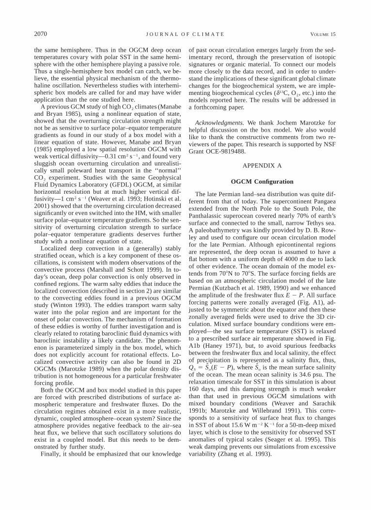
The late Permian land–sea distribution was quite dif-ferent from that of today. The supercontinent Pangaeaextended from the North Pole to the South Pole, thePanthalassic superocean covered nearly 70% of earth’ssurface and connected to the small, narrow Tethys sea.A paleobathymetry was kindly provided by D. B. Row-ley and used to configure our ocean circulation modelfor the late Permian. Although epicontinental regionsare represented, the deep ocean is assumed to have aflat bottom with a uniform depth of 4000 m due to lackof other evidence. The ocean domain of the model ex-tends from 708N to 708S. The surface forcing fields arebased on an atmospheric circulation model of the latePermian (Kutzbach et al. 1989, 1990) and we enhancedthe amplitude of the freshwater flux E 2 P. All surfaceforcing patterns were zonally averaged (Fig. A1), ad-justed to be symmetric about the equator and then thesezonally averaged fields were used to drive the 3D cir-culation. Mixed surface boundary conditions were em-ployed—the sea surface temperature (SST) is relaxedto a prescribed surface air temperature showed in Fig.A1b (Haney 1971), but, to avoid spurious feedbacksbetween the freshwater flux and local salinity, the effectof precipitation is represented as a salinity flux, thus,QS 5 So(E 2 P), where So is the mean surface salinityof the ocean. The mean ocean salinity is 34.6 psu. Therelaxation timescale for SST in this simulation is about160 days, and this damping strength is much weakerthan that used in previous OGCM simulations withmixed boundary conditions (Weaver and Sarachik1991b; Marotzke and Willebrand 1991). This corre-sponds to a sensitivity of surface heat flux to changesin SST of about 15.6 W m22 K21 for a 50-m-deep mixedlayer, which is close to the sensitivity for observed SSTanomalies of typical scales (Seager et al. 1995). Thisweak damping prevents our simulations from excessivevariability (Zhang et al. 1993).


FIG A1. Surface atmospheric forcing fields used to drive theOGCM: (a) surface wind stress, (b) surface air temperature, (c) andfreshwater forcing E 2 P.

APPENDIX B

Dimensional Dynamic Equations for theThree-Box Model

ˆdT ql ˆ ˆ ˆ ˆ5 l(T 2 T ) 1 (T 2 T )Al l d hdt 2Vl

ˆ|q | Kˆ ˆ ˆ ˆ ˆ1 (T 1 T 2 2T ) 1 (T 2 T )d h l h l22V Ll

Ml ˆ ˆ1 (T 2 T ) (B1)d lh 1 Hh

2ˆdT qh ˆ ˆ ˆ ˆ5 l(T 2 T ) 1 (T 2 T )Ah h l ddt 2Vh

ˆ|q | Kˆ ˆ ˆ ˆ ˆ1 (T 1 T 2 2T ) 1 (T 2 T )l d h l h22V Lh

Mh ˆ ˆ1 (T 2 T ) (B2)d hh 1 Hh

2

ˆdT q |q |d ˆ ˆ ˆ ˆ ˆ5 (T 2 T ) 1 (T 1 T 2 2T )h l h l ddt 2V 2Vd d

Ml ˆ ˆ1 (T 2 T )l dh 1 H2H

2

Mh ˆ ˆ1 (T 2 T ) (B3)h dh 1 H2H

2ˆ ˆdS FS q |q |l 0 ˆ ˆ ˆ ˆ ˆ5 1 (S 2 S ) 1 (S 1 S 2 2S )d h d h ldt h 2V 2Vl l

ˆ ˆK Mˆ ˆ ˆ ˆ1 (S 2 S ) 1 (S 2 S ) (B4)h l d l2L h 1 Hh

2ˆ ˆdS FS qh 0 ˆ ˆ5 2 1 (S 2 S )l ddt h 2Vh

|q | ˆ ˆ ˆ1 (S 1 S 2 2S )l d h2Vh

ˆ ˆK Mhˆ ˆ ˆ ˆ1 (S 2 S ) 1 (S 2 S ) (B5)l h d h2L h 1 Hh

2

ˆdS q |q |d ˆ ˆ ˆ ˆ ˆ5 (S 2 S ) 1 (S 1 S 2 2S )h l h l ddt 2V 2Vd d

Ml ˆ ˆ1 (S 2 S )l dh 1 H2H

2

Mh ˆ ˆ1 (S 2 S ). (B6)h dh 1 H2H

2

Here S0 is mean salinity of the ocean. At the air–seasurface there is no net salt flux so the total salinity ofthe three boxes is conserved. Hence, there are only fiveindependent dynamic variables.

APPENDIX C

Properties of Steady-State Solutions

For steady TM ( f . 0), the nondimensional meandensity difference between surface and deep ocean box-es can be obtained from Eqs. (7) to (12) and (6) as

f M 1 g fhDr 5 2 (C1)ld m M 1 M 1 g ff l h

f MlDr 5 . (C2)hd m M 1 M 1 g ff l h

From the above relations, we know that Drld , 0 andDrhd . 0 since f . 0, that is, for steady TM ( f . 0)


the low-latitude surface is always less dense than thedeep ocean, and the high surface is always denser thanthe deep ocean. Combining with the rules of convectiveadjustment, we can see that, for physically possiblesteady TM ( f . 0), no convection occurs in low lati-tudes (Ml 5 M) while strong convection happens inpolar regions (Mh 5 Msc). Substitute Ml 5 M, Mh 5Msc into Eq. (13), we can obtain the steady TM solutionsfor given parameters.

REFERENCES

Brass, G. W., J. R. Southam, and W. H. Peterson, 1982: Warm salinebottow water in the ancient ocean. Nature, 296, 620–623.

Budyko, M. I., and A. B. Ronov, 1979: Atmospheric evolution in thePhanerozoic. Geochem. Int., 16, 1–9.

Haney, R. L., 1971: Surface thermal boundary condition for oceancirculation models. J. Phys. Oceanogr., 1, 241–248.

Haupt, B., and D. Seidov, 2001: Warm deep-water ocean conveyorduring Cretaceous time. Geology, 29, 295–298.

Hotinski, R. M., K. L. Bice, L. R. Lump, R. G. Najjar, and M. A.Arthur, 2001: Ocean stagnation and end-Permian anoxia. Ge-ology, 29, 7–10.

Huang, R. X., 1994: Thermohaline circulation: Energetics and var-iability in a single-hemisphere basin model. J. Geophys. Res.,99, 12 471–12 485.

——, J. Luyten, and H. M. Stommel, 1992: Multiple equilibriumstates in combined thermal and saline circulation. J. Phys.Oceanogr., 22, 231–246.

Johnson, S. J., and Coauthors, 1992: Irregular glacial interstadialsrecorded in a new Greenland ice core. Nature, 359, 311–313.

Kozur, H. W., 1998: Some aspects of the Permian–Triassic boundary(PTB) and of the possible causes for the biotic crisis around thisboundary. Palaeogeogr., Palaeoclimatol., Palaeoecol., 143,227–272.

Kutzbach, J. E., and R. G. Gallimore, 1989: Pangaean climates: Mega-monsoons of the megacontinent. J. Geophys. Res., 94, 3341–3358.

——, P. J. Guetter, and W. M. Washington, 1990: Simulated circu-lation of an idealized ocean for Pangaean time. Paleoceanog-raphy, 5, 299–317.

Ledwell, J. R., A. J. Watson, and C. S. Law, 1993: Evidence for slowmixing across the pycnocline from an open-ocean tracer-releaseexperiment. Nature, 364, 701–703.

Manabe, S., and K. Bryan, 1985: CO2-induced change in a coupledocean–atmosphere model and its paleoclimatic implications. J.Geophys. Res., 90, 11 689–11 707.

——, and R. J. Stouffer, 1994: Multiple-century response of a coupledocean–atmosphere model to an increase of atmospheric carbondioxide. J. Climate, 7, 5–23.

Marotzke, J., 1989: Instabilities and multiple steady states of thethermohaline circulation. Oceanic Circulation Models: Combin-ing Data and Dynamics, D. L. T. Anderson and J. Willebrand,Eds., Kluwer Academic Publishers, 501–511.

——, 1997: Boundary mixing and the dynamics of three-dimensionalthermohaline circulations. J. Phys. Oceanogr., 27, 1713–1728.

——, and J. Willebrand, 1991: Multiple equalibria of the global ther-mohaline circulation. J. Phys. Oceanogr., 21, 1372–1385.

Marshall, J., and F. Schott, 1999: Open ocean deep convection: Ob-servations, models and theory. Rev. Geophys., 37, 1–64.

——, C. Hill, L. Perelman, and A. Adcroft, 1997a: Hydrostatic, quasi-hydrostatic, and nonhydrostatic ocean modeling. J. Geophys.Res., 102, 5733–5752.

——, A. Adcroft, C. Hill, L. Perelman, and C. Heisey, 1997b: Afinite-volume, incompressible Navier–Stokes model for studiesof the ocean on parallel computers. J. Geophys. Res., 102, 5753–5766.

Munk, M., and C. Wunsch, 1998: Abyssal recipes II: Energetics oftidal and wind mixing. Deep-Sea Res., 45, 1977–2010.

Pierce, D. W., T. P. Barnett, and U. Mikolajewicz, 1995: Competingroles of heat and freshwater flux in forcing thermohaline oscil-lations. J. Phys. Oceanogr., 25, 2046–2064.

Railsback, L. B., S. C. Ackerly, T. F. Anderson, and J. L. Cisne, 1990:Palaeontological and isotope evidence for warm saline deep wa-ters in Ordovician oceans. Nature, 343, 156–159.

Rooth, C., 1982: Hydrology and ocean circulation. Progress inOceanography, Vol. 11, Pergamon, 131–149.

Ruddick, B., and L. Q. Zhang, 1996: Qualitative behavior and non-oscillation of Stommel’s thermohaline box model. J. Climate, 9,2768–2777.

Seager, R., Y. Kushnir, and M. A. Cane, 1995: On heat flux boundaryconditions for ocean models. J. Phys. Oceanogr., 25, 3219–3230.

Stommel, H., 1961: Thermohaline convection with two stable regimesof flow. Tellus, 13, 224–230.

Taylor, E. L., T. N. Taylor, and N. R. Cuneo, 1992: The present isnot the key to the past: A polar forest from the Permian ofAntarctica. Science, 257, 1657–1677.

Toole, J. M., K. L. Polzin, and R. Schmitt, 1994: Estimates of dia-pycnal mixing in the abyssal ocean. Science, 264, 1120–1123.

Weaver, A. J., and E. S. Sarachik, 1991a: The role of mixed boundaryconditions in numerical models of the ocean’s climate. J. Phys.Oceanogr., 21, 1470–1493.

——, and ——, 1991b: Evidence for decadal variability in an oceangeneral circulation model: An advective mechanism. Atmos.–Ocean, 29, 197–231.

——, J. Marotzke, P. F. Cummins, and E. S. Sarachik, 1993: Stabilityand variability of the thermohaline circulation. J. Phys. Ocean-ogr., 23, 39–60.

Welander, P., 1982: A simple heat–salt oscillator. Dyn. Atmos. Oceans,6, 233–242.

Winton, M., 1993: Deep decoupling oscillations of the oceanic ther-mohaline circulation. Ice in the Climate System, NATO ASISeries, Vol. 112, Springer Verlag, 417–432.

——, and E. S. Sarachik, 1993: Thermohaline oscillations inducedby strong steady salinity forcing of ocean general circulationmodels. J. Phys. Oceanogr., 23, 1389–1410.

Wright, D. G., and T. F. Stocker, 1991: A zonally averaged model forthe thermohaline circulation. Part I: Model development and flowdynamics. J. Phys. Oceanogr., 21, 1713–1724.

Zhang, R., M. Follows, J. P. Grotzinger, and J. Marshall, 2001: Couldthe late Permian deep ocean have been anoxic? Paleoceanog-raphy, 16, 317–329.

Zhang, S., R. J. Greatbatch, and C. A. Lin, 1993: A reexaminationof the polar halocline catastrophe and implications for coupledocean–atmosphere modeling. J. Phys. Oceanogr., 23, 287–299.

Documents

Mechanisms of Thermohaline Mode Switching with Application ...paoc.mit.edu/paoc/papers/mode_switch.pdf · Mechanisms of Thermohaline Mode Switching with Application to ... It is found