Embed Size (px)
Citation preview

Mechanism Choice and Strategic Bidding in Divisible Good Auctions:
An Empirical Analysis of the Turkish Treasury Auction Market
Ali Hortacsu and David McAdams 1
October 6, 2010
1Hortacsu (corresponding author) is at the Department of Economics, University of Chicago, 1126 E. 59th
Street, Chicago, IL 60613. E-mail: [email protected]. McAdams is at the Fuqua School of Business
and the Economics Department, Duke University. Email: [email protected]. This paper is based on
(and replaces) Hortacsu’s earlier paper with the same title. He would like to thank his thesis advisors Patrick
Bajari, Lanier Benkard, Timothy Bresnahan, and Robert Wilson for their generous encouragement and support.
Bradley Efron, Glenn Ellison, Philip Haile, Jonathan Levin, Preston McAfee, Leonardo Rezende, and Frank
Wolak made important contributions to this research with their valuable comments and suggestions. Thanks
are also due to Berna Bayazitoglu for access to her dataset, and to Erdal Yılmaz of the Central Bank of Turkey,
Volkan Taskın of the Turkish Ministry of Treasury, Ahmet Arzan and Derya Tamerler for helpful discussions
about the Turkish Treasury auction system. We also acknowledge excellent research assistance by Julian Reif.
Financial support for this research was provided by a John M. Olin Dissertation Fellowship from SIEPR and
the Olin Program in Law and Economics and the NSF (SES-0449625).

Abstract
We propose an estimation method to bound bidders’ marginal valuations in discriminatory auctions
using individual bid-level data, and apply the method to data from the Turkish Treasury auction
market. Using estimated bounds on marginal values, we compute an upper bound on the inefficiency
of realized allocations as well as bounds on how much additional revenue could have been realized in
a counterfactual uniform price or Vickrey auction. We conclude that switching from a discriminatory
auction to a uniform price or Vickrey auction would not significantly increase revenue. Moreover, such
a switch would increase bidder expected surplus by at most 0.02%.
Keywords: Multi-unit auctions, divisible good or share auctions, Treasury auctions, structural econo-
metrics, nonparametric identification and estimation

1 Introduction
What is the most effective way for a Treasury to sell government securities? Since governments
sell about $4 trillion dollars worth of securities every year (Bartolini and Cottarelli (1997)), many
economists have tried to answer this question, interpreting “effectiveness” from both the revenue
maximization and efficiency standpoints. At least since Friedman (1960), the unanimous suggestion
of the profession has been to conduct the sale through an auction. Unfortunately there is much less
of a consensus among economists as to what the optimal auction mechanism should be, with theory
providing no clear answer.1
This paper begins to fill this gap in the literature by developing techniques to let the data decide
on the relative ranking of different auction mechanisms. Cross-country studies of Treasury practices
reveal that practitioners overwhelmingly prefer one mechanism over others: 39 out of 42 countries
surveyed by Bartolini and Cottarelli (1997) use the discriminatory auction mechanism, also known
as the “pay-as-bid” or “multiple-price” auction. In this auction format, bidders may submit multiple
price-quantity pairs as their bids, which trace out bid functions on the price-quantity plane. Treasury
officials aggregate individual bid functions and find where the aggregate bid function meets supply,
as in Figure 1(a). The revenue of the auctioneer is the area under the aggregate bid function up to
the market-clearing price. An alternative mechanism that has been the favorite of many economists,
including Friedman, is the uniform price auction.2 Here, winning bids are determined in the same
manner as in the discriminatory auction, but bidders pay the market-clearing price for all the units
they purchase. In this case, the auctioneer’s revenue is the rectangle defined by the total quantity
being sold and the market-clearing price, as shown in Figure 1(b).
Building on the seminal work of Wilson (1979), we model bidder behavior in a discriminatory
auction as an incomplete information game. As long as bids are strictly downward-sloping demand
1See the survey by Nandi (1997). Ausubel and Cramton (1997) and Engelbrecht-Wiggans and Kahn (1998) show
that the discriminatory and uniform price auctions cannot be generally ranked on either efficiency or revenue grounds,
even given independent private values. In particular, the celebrated revenue equivalence results of Vickrey (1961) and
the revenue ranking results of Milgrom and Weber (1982) do not apply to share auctions.2An important advantage of the uniform price auction, cited by many economists, is that it invites wider participation
since all winning bidders pay the same price and hence do not need to invest in predicting the market-clearing price.
As Friedman (1991) argued, by contrast,“[the discriminatory auction] tends to limit the market to specialists” who may
also be more likely to collude.
1

schedules, the model yields a first-order necessary condition in which the price bid for a given quantity
equals the bidder’s marginal value less an oligopsonistic “mark-down” that depends on the inverse
elasticity of the residual supply function each bidder expects to face. Inverting this mark-down rule
identifies bidders’ unobserved marginal valuations, and allows an econometrician to conduct coun-
terfactual calculations in which the revenue performance of a uniform price or Vickrey auction can
be compared to the performance of a discriminatory auction. In practice, however, observed bids
are not strictly downward-sloping and bidder values are not point-identified under the hypothesis of
equilibrium play. Instead, we provide a methodology to compute upper and lower bounds on bidders’
valuations, and use these bounds for counterfactual analysis.
We apply this framework to data from the Turkish Treasury, covering 3-month T-bill auctions
between 1991 and 1993, to explore how much additional revenue the Treasury might have generated if
it had switched to either a uniform price or Vickrey auction. We conclude that switching to either of
these auction formats would not have significantly increased revenue or (gross) bidder surplus. More
precisely, we can not reject (ex ante) revenue equivalence between the discriminatory auction and a
hypothetical auction that yields strictly higher revenue than the uniform price or Vickrey auction. By
our point estimate, the switch from a discriminatory to a uniform price auction would lead to a gain of
expected revenue that is at most 0.12% of the realized revenue (about $14.4 million, considering that
$12 billion of debt was auctioned in this period). However, taking sampling variation into account, we
can not reject the hypothesis that such a switch would lead to no difference in revenue, even under the
best case scenario for the uniform price auction. We also find that the discriminatory auction itself
was close to fully efficient, estimating that switching to an efficient mechanism would have increased
bidder expected surplus by at most 0.02% over the 3-year period.
This paper differs from much of the past literature comparing Treasury auction mechanisms, in
that we employ a structural model of strategic bidding. Past work has focused almost exclusively on
“policy experiments” in which different auction formats have been used in different time periods or in
the sale of securities of different maturities. These studies have compared the differential between the
auction price and the resale or forward (“when-issued”) market price of the security across separate
samples of discriminatory and uniform price auctions.3 The assumption implicit in this line of research
is that bidders’ true valuations for the security are better reflected in resale or forward markets than in
3See Umlauf (1993), Simon (1994), Nyborg and Sundaresan (1996) and Malvey and Archibald (1998).
2

the auction. Hence, the claim is that smaller differentials between the auction price and the transaction
prices in secondary markets reflects better surplus extraction by the auctioneer. The validity of this
comparison relies heavily on the assumption that one can control for factors that may have changed
between the end of the auction and the start of trade in the resale market, including the release of new
information that might impact bidders’ valuations of the security. The advantage of the structural
approach taken here is that estimation of model primitives allows us to construct counterfactual
simulations in which bidders’ ex ante information sets are fixed. Furthermore, the policy experiment
studies cited above have relied on aggregated price data from the auctions, whereas we utilize bidder
level data. This allows us to assess the distributional aspects of a policy intervention that changes the
mechanism.
The most closely related paper is Heller and Lengwiler (1998), who uses a similar first-order
condition to estimate the amount of (counterfactual) bid-shading in a discriminatory auction.4 How-
ever, their model is based on Nautz (1995), which abstracts from some important aspects of strategic
bidding. In particular, their model predicts that all bidders will shade their bids by the same amount,
regardless of their market power.5 Also, Heller and Lengwiler (1998) model bidders’ expectation about
the market-clearing price distribution using the distribution of past market-clearing prices, and hence
do not make use of the information contained in individual bids to investigate the strategic effect of
each bidder on the equilibrium market-clearing price distribution.
Like this paper, Fevrier, Preget and Visser (2002) uses a structural approach to estimate a
strategic model of bidding in the discriminatory auction. Their paper differs in that they estimate a
parametric model with symmetric common values, while we estimate a non-parametric model assuming
private values.
In work that follows and builds upon an earlier version of this paper (Hortacsu (2002))6, Kang
and Puller (2008) conducts a counterfactual revenue comparison of the discriminatory and uniform
4The closely related idea of using first-order conditions to reconstruct unobserved marginal cost functions from ob-
served supply decisions has been present in the industrial organization literature at least since Rosse (1970) and Bresnahan
(1981).5Other early work analyzed Treasury auctions within a strategic equilibrium framework but, due to the analytical
and computational difficulties associated with divisible-good auctions, focused on models of single-unit auctions. See e.g.
Nyborg, Rydqvist and Sundaresan (2002) and Gordy (1994).6The earlier version of the paper developed identification results in the case analyzed by Wilson (1979) where bidders
submit continuous demand curves. Here, we consider the more realistic situation where bidders submit step functions.
3

price auctions, using data from discriminatory Korean Treasury auctions. They find that the discrim-
inatory auction yielded statistically greater expected revenue and a more efficient allocation of the
securities at auction, although these effects were each fairly small. Also related is Kastl (2006), who
uses a set of necessary conditions for optimal bidding to infer bounds on bidders’ values in the Czech
Treasury’s uniform price auction. He concludes that the uniform price auction performs well, in that
it “failed to extract at most 0.03% (in terms of the annual yield of T-bills) worth of expected surplus
while implementing an allocation resulting in almost all of the efficient surplus”.
This paper also adds to the literature on structural econometric modeling of auctions. In
particular, we extend the nonparametric identification and estimation framework of Elyakime, Laffont,
Loisel and Vuong (1994) and Guerre, Perrigne and Vuong (2000) to divisible good auctions, and offer
an empirical algorithm with low computational demands. The statistical properties of our estimation
algorithm are also discussed.
The outline of the paper is as follows. Section 2 presents a model of strategic bidding in a
discriminatory auction. Section 3 discusses how this model can be used as an empirical device to
estimate bidders’ unobserved marginal valuations. Section 4 provides background information on the
institutional setup of the Turkish Treasury auction market and reports descriptive statistics from the
data, including evidence on inventory/liquidity concerns as a source of private information. In Section
5, we use bidding data from the Turkish Treasury bill auctions between October 1991 and October
1993 to estimate bidders’ marginal valuations. Using these estimates, we conduct counterfactual
comparisons of the discriminatory, uniform price and Vickrey auctions. Section 6 discusses several
extensions, while Section 7 concludes.
2 Modeling and identification framework
Our theoretical model is based on Wilson (1979)’s share auction framework and, more specifically,
Swinkels (2001)’s multi-unit auction model. There are T auctions. Each auction t = 1, ..., T is a
discriminatory auction of Qt indivisible units with N potential bidders. As in Swinkels (2001), we
allow for the possibility that supply is random, or that a random subset of the bidders may have zero
values and choose not to participate. (By assumption, bidding is costless.)
4

Assumptions on bidder values. Bidders in each auction are symmetric and risk-neutral with
independent private values (IPV). Each player desires up to ymax objects, with non-increasing marginal
value schedule vit(.) = (vit(1), ..., vit(ymax)) ∈ V having a well-defined density over Rymax
. Let dit(.)
denote the demand schedule corresponding to vit(.), i.e. dit(p) = max{y : vit(y) ≥ p}.
Discriminatory auction rules. A bid is a non-increasing price schedule pit(.) = (pit(1), ..., pit(ymax))
or, equivalently, a non-increasing bid schedule yit(.) defined by yit(p) ≡ max{0 ≤ y ≤ ymax : pit(y) ≤
p}. (By convention, set pit(0) = ∞ and pit(y) = 0 for all y > ymax.) A range of consecutive quantities
may be bid at the same price. If so, we refer to this range of quantities as a “step”.
Bidder i pays his unit-bid on every unit that he wins. At any price p, the (random) residual
supply available to bidder i is Qt −∑
j 6=i yjt(p, vjt(.)), where yjt(., vjt(.)) denotes bidder j’s strategy
in auction t, as a function of his marginal value schedule. (We will also use inverse demand notation
pit(., vit(.)) for strategies, as convenient.) In particular, if bidder i submits a bid pit(.) such that
pit(y) = p, bidder i wins at least quantity y as long as his residual supply at price p is greater than or
equal to y, i.e. with probability7
Git(y; p) = Pr
Qt −∑
j 6=i
yjt(p, vjt(.)) ≥ y
. (1)
Assumptions on strategies. In each auction t, bidders play symmetric pure strategies pt(., vit(.)) so
that Git(y; p) = Gt(y; p) for all i. Further, bidders’ strategies constitute a Bayesian Nash equilibrium.
Interim expected payoffs in the discriminatory auction take the form
Πt(p(.), vit(.)) =
ymax∑
y=1
Gt(y; p(y))(vit(y) − p(y)). (2)
The equilibrium assumption may be restated as Πt(pt(., vit(.)), vit(.)) ≥ Πt(p(.), vit(.)) for all bids p(.)
and all marginal value schedules vit(.) ∈ V.
To simplify the exposition, we will henceforth drop notation specifying the bidder i and the
auction t, except where such notation is needed for clarity.
7Implicit in this formulation is a simplifying assumption that there are no “ties”, i.e. at most one bidder is rationed.
In practice, given a finite set of prices so that such ties occur with positive probability, we modified each bidder’s winning
probability (1) to account for the effects of rationing.
5
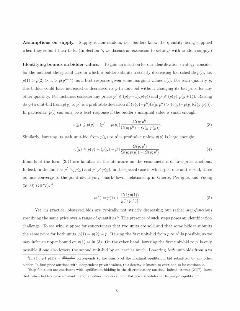
Assumptions on supply. Supply is non-random, i.e. bidders know the quantity being supplied
when they submit their bids. (In Section 5, we discuss an extension to settings with random supply.)
Identifying bounds on bidder values. To gain an intuition for our identification strategy, consider
for the moment the special case in which a bidder submits a strictly decreasing bid schedule p(.), i.e.
p(1) > p(2) > ... > p(ymax), as a best response given some marginal values v(.). For each quantity y,
this bidder could have increased or decreased its y-th unit-bid without changing its bid price for any
other quantity. For instance, consider any prices ph ∈ (p(y−1), p(y)) and pl ∈ (p(y), p(y+1)). Raising
its y-th unit-bid from p(y) to ph is a profitable deviation iff (v(y)−ph)G(y; ph) > (v(y)−p(y))G(y; p(.)).
In particular, p(.) can only be a best response if the bidder’s marginal value is small enough:
v(y) ≤ p(y) + (ph − p(y))G(y; ph)
G(y; ph) − G(y; p(y)). (3)
Similarly, lowering its y-th unit-bid from p(y) to pl is profitable unless v(y) is large enough:
v(y) ≥ p(y) + (p(y) − pl)G(y; pl)
G(y; p(y)) − G(y; pl). (4)
Bounds of the form (3,4) are familiar in the literature on the econometrics of first-price auctions.
Indeed, in the limit as ph ց p(y) and pl ր p(y), in the special case in which just one unit is sold, these
bounds converge to the point-identifying “mark-down” relationship in Guerre, Perrigne, and Vuong
(2000) (GPV): 8
v(1) = p(1) +G(1; p(1))
g(1; p(1)). (5)
Yet, in practice, observed bids are typically not strictly decreasing but rather step-functions
specifying the same price over a range of quantities.9 The presence of such steps poses an identification
challenge. To see why, suppose for concreteness that two units are sold and that some bidder submits
the same price for both units, p(1) = p(2) = p. Raising the first unit-bid from p to ph is possible, so we
may infer an upper bound on v(1) as in (3). On the other hand, lowering the first unit-bid to pl is only
possible if one also lowers the second unit-bid by at least as much. Lowering both unit-bids from p to
8In (5), g(1; p(1)) = dG(1;p(1)dp
corresponds to the density of the maximal equilibrium bid submitted by any other
bidder. In first-price auctions with independent private values, this density is known to exist and to be continuous.9Step-functions are consistent with equilibrium bidding in the discriminatory auction. Indeed, Anwar (2007) shows
that, when bidders have constant marginal values, bidders submit flat price schedules in the unique equilibrium.
6

pl = p is a profitable deviation iff∑
y=1,2(v(1)−pl)G(y; pl) >∑
y=1,2(v(y)−p)G(y; p). Note that, since
bidder values are by assumption non-increasing (v(1) ≥ v(2)), this deviation is profitable whenever
v(1) is large enough that (v(1)−pl)∑
y=1,2 G(y; pl) > (v(1)−p)∑
y=1,2 G(y; p). In particular, p(.) can
only be a best response if
v(1) ≥ p + (p − pl)
∑y=1,2 G(y; pl)
∑y=1,2 G(y; p) −
∑y=1,2 G(y; pl)
. (6)
Unfortunately, as ph ց p(y) and pl ր p(y), the upper and lower bounds on v(1) derived in this way
do not converge to one another.
In other words, because of the constraint that bids must be non-increasing schedules, bidder
values in the discriminatory auction are not point-identified by the necessary conditions of optimal
bidding given independent private values. Indeed, a bidder may find the same bid to be a best
response given many different marginal value schedules. (For a simple example, see Example 2 in
McAdams (2008).) Thus, the nature of the inference we are going to draw from our data regarding
the distribution of the structural parameter v(.) is incomplete, as in Haile and Tamer (2003).
Proposition 1 provides the upper and lower bounds on marginal values that we will use later in
our empirical analysis.
Proposition 1. Consider any bid p(.) and any step [y, y] of that bid, i.e. p(y − 1) > p(y) = p(y) >
p(y + 1), an example of which is shown in Figure 2. Bid p(.) can only be a best response if, for all
y ∈ [y, y] and all 0 < ∆ ≤ min{p(y − 1) − p(y), p(y) − p(y + 1)}, marginal value v(y) satisfies
v(y) ≤ v(y; p(.)) = p(y) + ∆ +∆
∑yq=y G(q; p(y))
∑yq=y [G(q; p(y) + ∆) − G(q; p(y))]
. (7)
v(y) ≥ v(y; p(.)) = p(y) +∆
∑yq=y G(q; p(y) − ∆)
∑yq=y [G(q; p(y)) − G(q; p(y) − ∆)]
(8)
Proof. Suppose for the sake of contradiction that v(y) > v(y; p(.)). We will show that it is a profitable
deviation for the bidder to raise his unit-bids on all quantities [y, y] from p(y) to p(y)+∆, as illustrated
by the deviation denoted by up-arrows in Figure 2. Such a deviation has no impact on the bidder’s
likelihood of winning or payment for any quantity outside [y, y], but both increases the likelihood of
winning these units and increases the price paid for them upon winning. For each quantity q ∈ [y, y],
bidding p(y) is enough to win that quantity with probability G(q; p(y)). In these cases, bidding p(y)+∆
causes the bidder to pay ∆ more for that unit. On the other hand, if bidding p(y) + ∆ is enough
7
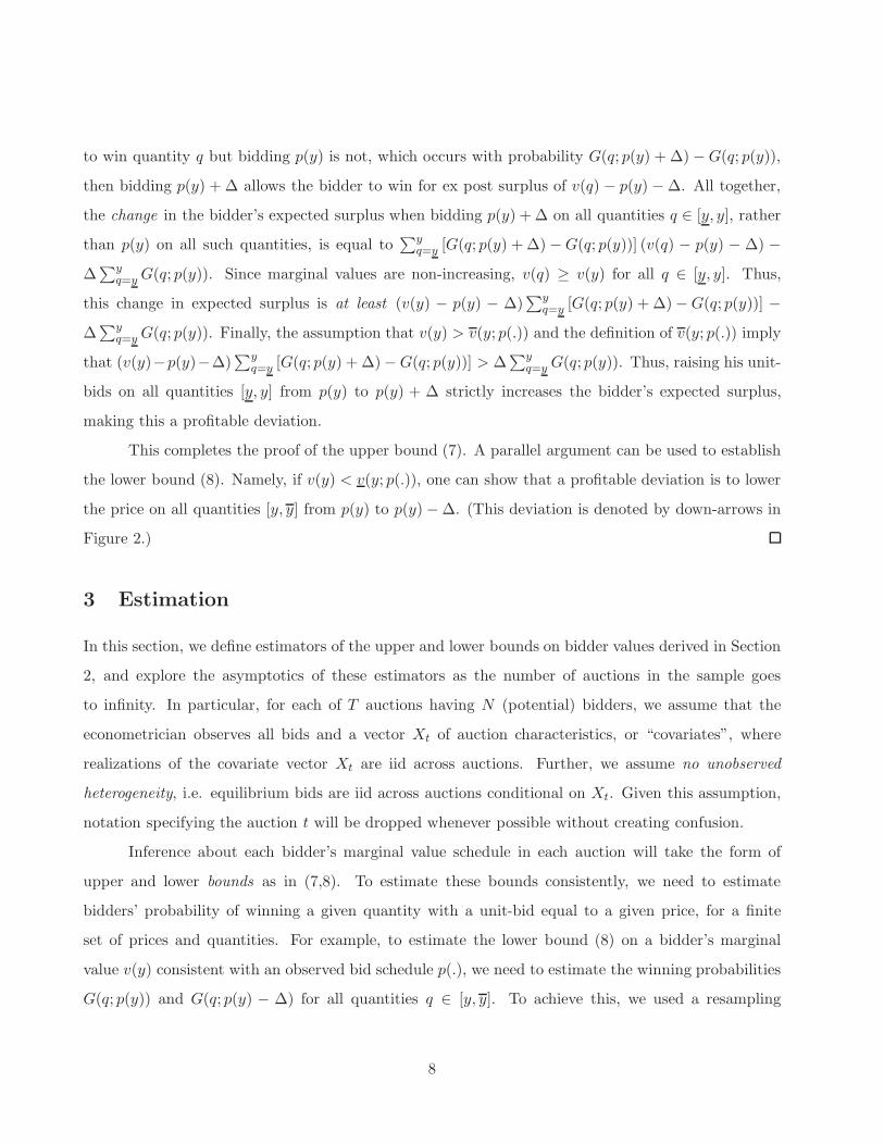
to win quantity q but bidding p(y) is not, which occurs with probability G(q; p(y) + ∆) − G(q; p(y)),
then bidding p(y) + ∆ allows the bidder to win for ex post surplus of v(q) − p(y) − ∆. All together,
the change in the bidder’s expected surplus when bidding p(y) + ∆ on all quantities q ∈ [y, y], rather
than p(y) on all such quantities, is equal to∑y
q=y [G(q; p(y) + ∆) − G(q; p(y))] (v(q) − p(y) − ∆) −
∆∑y
q=y G(q; p(y)). Since marginal values are non-increasing, v(q) ≥ v(y) for all q ∈ [y, y]. Thus,
this change in expected surplus is at least (v(y) − p(y) − ∆)∑y
q=y [G(q; p(y) + ∆) − G(q; p(y))] −
∆∑y
q=y G(q; p(y)). Finally, the assumption that v(y) > v(y; p(.)) and the definition of v(y; p(.)) imply
that (v(y)−p(y)−∆)∑y
q=y [G(q; p(y) + ∆) − G(q; p(y))] > ∆∑y
q=y G(q; p(y)). Thus, raising his unit-
bids on all quantities [y, y] from p(y) to p(y) + ∆ strictly increases the bidder’s expected surplus,
making this a profitable deviation.
This completes the proof of the upper bound (7). A parallel argument can be used to establish
the lower bound (8). Namely, if v(y) < v(y; p(.)), one can show that a profitable deviation is to lower
the price on all quantities [y, y] from p(y) to p(y) − ∆. (This deviation is denoted by down-arrows in
Figure 2.)
3 Estimation
In this section, we define estimators of the upper and lower bounds on bidder values derived in Section
2, and explore the asymptotics of these estimators as the number of auctions in the sample goes
to infinity. In particular, for each of T auctions having N (potential) bidders, we assume that the
econometrician observes all bids and a vector Xt of auction characteristics, or “covariates”, where
realizations of the covariate vector Xt are iid across auctions. Further, we assume no unobserved
heterogeneity, i.e. equilibrium bids are iid across auctions conditional on Xt. Given this assumption,
notation specifying the auction t will be dropped whenever possible without creating confusion.
Inference about each bidder’s marginal value schedule in each auction will take the form of
upper and lower bounds as in (7,8). To estimate these bounds consistently, we need to estimate
bidders’ probability of winning a given quantity with a unit-bid equal to a given price, for a finite
set of prices and quantities. For example, to estimate the lower bound (8) on a bidder’s marginal
value v(y) consistent with an observed bid schedule p(.), we need to estimate the winning probabilities
G(q; p(y)) and G(q; p(y) − ∆) for all quantities q ∈ [y, y]. To achieve this, we used a resampling
8

approach that provides consistent estimates of such winning probabilities, as the number of auctions
T goes to infinity while holding fixed the number of bidders per auction.
3.1 A resampling approach
Since bidders are presumed to have private values, each bidder i cares about others’ bidding strategies
only insofar as they affect the distribution of bidder i’s residual supply. Our approach to estimate
this distribution is based on resampling from the observed set of bids.10 Consider for the moment the
special case in which all T auctions in the sample have identical covariates. The following “resampling”
procedure, illustrated in Figures 3-4, greatly simplifies the estimation problem. (Section 3.2 provides
full details and generalizes this procedure to settings with auction-specific covariates.)
1. Fix bidder i and a bid pi(.) made by this bidder. (In Figures 3-4, this is bidder #2 and its bid
in auction #1.)
2. Draw a random subsample of N − 1 bid vectors with replacement from the sample of NT bids
in the data set.
3. Construct bidder i’s realized residual supply were others to submit these bids, to determine the
realized market-clearing price given i’s bid pi(.), as well as whether bidder i would have won
quantity y at price p for all (y, p).
Repeating this process many times allows one to consistently estimate each of bidder i’s winning
probabilities G(y; p), simply as the fraction of all subsamples given which bidder i would have won a
y-th unit at price p.
3.2 Estimation method
In this section, we formally define our estimators of the upper and lower bounds (7,8) on bidder
i’s marginal value for quantity y, when observed submitting bid schedule p(.). We also discuss the
asymptotic properties of these estimators, as the number of auctions T in the sample goes to infinity.
10An alternative approach developed in the first-price auction literature (see e.g. Paarsch (1992) and Laffont, Ossard
and Vuong (1995)) is to explicitly invert the equilibrium mapping from values to bids to form a likelihood function for
the observed data. Unfortunately, such a “direct estimation strategy” is not yet feasible for the discriminatory auction
since its equilibrium mapping has not been characterized.
9

The estimator. Let y(., v(.), x,N) denote each bidder’s bid (expressed as a demand function) given
private marginal value schedule v(.), in an auction having covariates x and N bidders. Exploiting the
symmetry assumption,11 and assuming that supply is known, the winning probabilities in this auction
can be expressed as
G(y; p|x,N) = Pr
N−1∑
j=1
yt(p, vj(.), x) ≤ Q − y|x
(9)
=
∫...
∫
︸ ︷︷ ︸N−1
1{
N−1∑
j=1
yj ≤ Q − y}
N−1∏
j=1
dF (yj ; p|x,N) (10)
= E[1{
N−1∑
j=1
yj ≤ Q − y}|x,N ] (11)
where F (y; p|x) = Pr(y(p, v(.), x) ≤ y|x) is the probability that a bidder will demand at most quantity
y at price p, and dF (y; p|x) = Pr(y(p, v(.), x) = y|x).
In the simplest case, where all T auctions in the data set have identical covariates and N bidders,
we can estimate F (y; p) by the empirical cdf
F T (y; p) =1
NT
T∑
t=1
N∑
j=1
1 {yjt(p) < y} (12)
and plug the empirical cdf into equation (9) to obtain an estimate of the winning probability:
GT (y; p) =
∫...
∫
︸ ︷︷ ︸N−1
1{N−1∑
j=1
yj ≤ Q − y}N−1∏
j=1
dF T (yj; p). (13)
Note that with the empirical cdf F T (yj; p), the above estimator is equivalent to:
GT (y; p) =1
(NT )N−1
NT∑
j1=1
. . .
NT∑
jN−1=1
1{yj1(p) + . . . yjN−1
(p) ≤ Q − y}
(14)
i.e. an average of all possible (N − 1)-fold sums of the NT bids, {yjt(p), j = 1 . . . N, t = 1 . . . T}.
This is a V-statistic (Lehmann (1999), p. 387) with kernel function 1{∑N−1
j=1 yj(p) ≤ Q − y}
.
Since this kernel function is bounded, as T → ∞, GT (y; p) is pointwise (in y) consistent and asymptot-
ically normal (Lehmann (1999), Theorem 6.2.2, p.389). Asymptotic variance estimates are provided
11Extending the method of this section to allow for asymmetric bidders and/or asymmetric strategies is straightforward.
Simply estimate the bidder-specific winning probabilities Git(y; p|x,N) in terms of bidder-specific Fjt(y; p|x,N) for all
j 6= i.
10

by Lehmann (1999), though inference can also be conducted using the bootstrap (Bickel and Freedman
(1981)).
In the more realistic case where auctions vary in their covariates Xt and number of bidders Nt,
we can estimate the conditional cdf F (y; p|x, n) by
F T (y; p|x, n) =T∑
t=1
K(Xt−xhx
T, Nt−n
hnT
)∑T
t′=1 K(Xt′−x
hxT
,Nt′−n
hnT
)
Nt∑
j=1
1 {yjt(p) < y}
Nt(15)
where K(x, n) is a kernel function, and hxT and hn
T are bandwidth parameters. The analog of (13) is
then:
GT (y; p|x, n) =
∫...
∫
︸ ︷︷ ︸n−1
1{
n−1∑
j=1
yj ≤ Q − y}
n−1∏
j=1
dF T (yj; p|x, n). (16)
This is equivalent to the conditional V-statistic,
GT (y; p|x, n) =
∑N(T )j1=1 . . .
∑N(T )jn−1=1 1{yj1(p) + . . . yjn−1(p) ≤ Q − y}Πn−1
k=1K(
x−Xjk
hxT
,n−Njk
hnT
)
∑N(T )j1=1 . . .
∑N(T )jn−1=1 Πn−1
k=1K(
x−Xjk
hxT
,n−Njk
hnT
) (17)
as in Example 4 of Falk and Reiss (1992), where N(T ) =∑T
t=1 Nt and (Xjk, Njk
) are the covari-
ate/number of bidders corresponding to the bid function yjk(p).
In the appendix, we show that (17) has the same probability limit and limiting distribution as
the closely related conditional U-statistic:
GT (y; p|x, n) =
∑(j1,...,jn−1) 1{yj1(p) + . . . yjn−1(p) ≤ Q − y}Πn−1
k=1K(
x−Xjk
hxT
,n−Njk
hnT
)
∑(j1,...,jn−1)
Πn−1k=1K
(x−Xjk
hxT
,n−Njk
hnT
) (18)
where the sum is indexed over all (n − 1)-tuples (j1, . . . , jn−1) with distinct elements taken from
1, . . . , N(T ). The argument is based on observing that (17) and (18) can be expressed as the ratio of
two unconditional V- and U-statistics, respectively. The asymptotic equivalence of unconditional U-
and V- statistics are well-known (see, e.g. Lehmann (1999)).
The representation of the estimator as a conditional U-statistic is convenient, as Stute (1991)
obtains the asymptotic normality (Theorem 1) and consistency (Theorem 2) of (18) around G(y; p|x, n)
(equation 11). The main conditions are that: (i) the density of yj(p) is continuous and strictly positive,
(ii) (hnT , hx
T ) → 0, (ThnT , Thx
T ) → ∞, and (iii) (T 1/5hnT , T 1/5hx
T ) → 0 for the asymptotic bias of the
kernel estimator to vanish.12 It is important to note that even with moderate sized T , computing (18)
12Stute (1991) also imposes a number of mild restrictions on the form of the kernel function K(.) for consistency – see
conditions (ii) and (iii) of his Theorem 2.
11
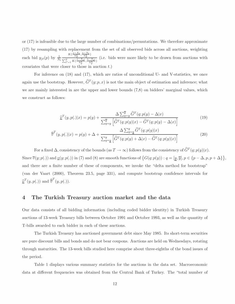
or (17) is infeasible due to the large number of combinations/permutations. We therefore approximate
(17) by resampling with replacement from the set of all observed bids across all auctions, weighting
each bid yjt(p) by 1Nt
K(x−Xt
hxT
,n−Nt
hnT
)
PTt′=1
K(x−X
t′
hxT
,n−N
t′
hnT
)(i.e. bids were more likely to be drawn from auctions with
covariates that were closer to those in auction t.)
For inference on (18) and (17), which are ratios of unconditional U- and V-statistics, we once
again use the bootstrap. However, GT (y; p, x) is not the main object of estimation and inference; what
we are mainly interested in are the upper and lower bounds (7,8) on bidders’ marginal values, which
we construct as follows:
vT (y, p(.)|x) = p(y) +∆
∑yq=y GT (q; p(y) − ∆|x)
∑yq=y
[GT (q; p(y)|x) − GT (q; p(y) − ∆|x)
] (19)
vT(y, p(.)|x) = p(y) + ∆ +
∆∑y
q=y GT (q; p(y)|x)
∑yq=y
[GT (q; p(y) + ∆|x) − GT (q; p(y)|x)
] (20)
For a fixed ∆, consistency of the bounds (as T → ∞) follows from the consistency of GT (q; p(y)|x).
Since v(y; p(.)) and v(y; p(.)) in (7) and (8) are smooth functions of{G(q; p(y)) : q = [y, y], p ∈ {p − ∆, p, p + ∆}
},
and there are a finite number of these of components, we invoke the “delta method for bootstrap”
(van der Vaart (2000), Theorem 23.5, page 331), and compute bootstrap confidence intervals for
vT (y, p(.)) and vT(y, p(.)).
4 The Turkish Treasury auction market and the data
Our data consists of all bidding information (including coded bidder identity) in Turkish Treasury
auctions of 13-week Treasury bills between October 1991 and October 1993, as well as the quantity of
T-bills awarded to each bidder in each of these auctions.
The Turkish Treasury has auctioned government debt since May 1985. Its short-term securities
are pure discount bills and bonds and do not bear coupons. Auctions are held on Wednesdays, rotating
through maturities. The 13-week bills studied here comprise about three-eighths of the bond issues of
the period.
Table 1 displays various summary statistics for the auctions in the data set. Macroeconomic
data at different frequencies was obtained from the Central Bank of Turkey. The “total number of
12
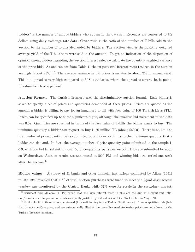
bidders” is the number of unique bidders who appear in the data set. Revenues are converted to US
dollars using daily exchange rate data. Cover ratio is the ratio of the number of T-bills sold in the
auction to the number of T-bills demanded by bidders. The auction yield is the quantity weighted
average yield of the T-bills that were sold in the auction. To get an indication of the dispersion of
opinion among bidders regarding the auction interest rate, we calculate the quantity-weighted variance
of the price bids. As one can see from Table 1, the ex post real interest rates realized in the auction
are high (about 23%).13 The average variance in bid prices translates to about 2% in annual yield.
This bid spread is very high compared to U.S. standards, where the spread is several basis points
(one-hundredth of a percent).
Auction format. The Turkish Treasury uses the discriminatory auction format. Each bidder is
asked to specify a set of prices and quantities demanded at these prices. Prices are quoted as the
amount a bidder is willing to pay for an imaginary T-bill with face value of 100 Turkish Liras (TL).
Prices can be specified up to three significant digits, although the smallest bid increment in the data
was 0.02. Quantities are specified in terms of the face value of T-bills the bidder wants to buy. The
minimum quantity a bidder can request to buy is 50 million TL (about $6000). There is no limit to
the number of price-quantity pairs submitted by a bidder, or limits to the maximum quantity that a
bidder can demand. In fact, the average number of price-quantity pairs submitted in the sample is
6.9, with one bidder submitting over 60 price-quantity pairs per auction. Bids are submitted by noon
on Wednesdays. Auction results are announced at 5:00 PM and winning bids are settled one week
after the auction.14
Bidder values. A survey of 51 banks and other financial institutions conducted by Alkan (1991)
in late 1989 revealed that 42% of total auction purchases were made to meet the liquid asset reserve
requirements monitored by the Central Bank, while 37% were for resale in the secondary market,
13Berument and Malatyali (1999) argue that the high interest rates in this era are due to a significant infla-
tion/devaluation risk premium, which was partly justified by a devaluation of the Turkish lira in May 1994.14Unlike the U.S., there is no when-issued (forward) trading in the Turkish T-bill market. Non-competitive bids (bids
that do not specify a price, and are automatically filled at the prevailing market-clearing price) are not allowed in the
Turkish Treasury auctions.
13
10% were to fill customer orders, and the remaining 10% were to fulfill collateral requirements,15 for
investment funds administered by the bank, and for buy-and-hold purposes.
In the period studied, at least 30% of bank portfolios had to be held as government bonds and
bills, with an average maturity of 210 days. Failure to comply with this requirement resulted in mone-
tary fines and could lead to a suspension of bank operations. Bidders’ idiosyncratic inventory/liquidity
needs therefore constitute an important source of private information in these auctions. Such private
information generates a private value if – conditional on publicly available information on the state of
the economy and especially the money markets/banking sector – learning about competing bidders’
inventory/liquidity needs does not affect a bidder’s assessment of its own inventory/liquidity needs
going into an auction.16
While resale incentives are also important for bidders’ demand of Treasury securities generally,
such incentives might be less pronounced in 13-week T-bill auctions due to their short maturity.17
The main venue for trading in government securities is the Istanbul Stock Exchange Bonds and Bills
Market (ISEBBM). Using daily transaction data from the ISEBBM, we calculated that, on average,
4% of the total volume of auctioned Treasury bills are traded on the ISE in a 3-day post-auction
window. If, as this seems to suggest, there is not a lot of liquidity in the resale market for T-bills
compared to the primary auction market, common values might be a poor model of bidder values for
these securities. We should note, however, that trading volumes on the ISEBBM showed a strong
growth trend during the period. Further, ISEBBM was not the only resale market available to the
bidders, who could also participate in over-the-counter deals. Unfortunately, we do not have access to
data on these transactions to assess their importance.
Although we believe that a private-values model of bidder values is a reasonable approximation
in the context of 13-week Turkish T-bill auctions, we would like to let the data decide on the appropriate
specification. Unfortunately, existing approaches to testing the private-values assumption do not apply
15The primary source of short-term funding for Turkish banks is the interbank money market, where banks engage in
short-term borrowing (“repo”) or lending (“reverse repo”), using Treasury securities as collateral.16In a private-values environment, bidders may still find information about their competitors’ reserve requirements
and liquidity states valuable, as noted by Alkan (1991). Although such information does not affect a bidder’s demand
for the security being auctioned, it gives the bidder a strategic advantage in the auction, as observed by Hortacsu and
Sareen (2005) and Hortacsu and Kastl (2008).17Haile (2001) provides related evidence in the context of timber auctions, that the role of resale decreases when time
horizons are shorter.
14

in our setting. In a recent paper, Hortacsu and Kastl (2008) provides a formal method to test for
the null hypothesis of private values in the Bank of Canada’s three-month treasury-bill auctions, and
fail to reject private values in that application. However, Hortacsu and Kastl’s testing strategy relies
heavily on a specific institutional feature of the Canadian market that is not present in the Turkish
market. In single-unit auctions, various tests of common-value and private-value specifications have
been developed that exploit the “winner’s curse” effect. These tests examine how the distribution of
bids changes in response to exogenous changes in the number of bidders in the auction. See Paarsch
(1992), Hendricks, Pinkse and Porter (2003), Haile, Hong and Shum (2003), Athey and Haile (2002)
for discussions and various implementations. However, an extension of this testing strategy to divisible
good/multi-unit auction models has not been developed.
Alkan (1991) reports as well that bidders find the following bits of information as being useful in
their bidding decision (most important listed first): Treasury’s borrowing requirements and repayment
schedule, liquidity in money markets, the bidder’s own liquid asset reserve requirement and the reserve
positions of other bidders, conversations with other bidders, and results of previous auctions. The fact
that information about supply was most important to bidders could be consistent with either private
or common values. In particular, banks who enter the auction primarily to meet their liquid asset
reserve requirements need this information as a critical input when determining what price to bid for
their minimum required quantity.
Supply. In the period we study, October 1991 to October 1993, the Treasury followed two different
procedures when determining the quantity of bills to supply. Beginning in February 1993, in auctions
#18-#27, the Treasury pre-announced the quantity in its 3- and 6-month Treasury bill auctions.18
Before then, in auctions #1-#17, the total quantity of bills to be sold was not announced until after bids
were submitted. Nonetheless, bank managers that we have interviewed claimed they could estimate
the supply of Treasury bills quite accurately by tracking debt service requirements of the Treasury,
and through contacts in the Treasury. As a reasonable approximation, we will assume that bidders
know the quantity to be supplied before the bidding in all auctions. However, since uncertainty about
supply could have been important in auctions #1-#17, we will also discuss an extension in which we
18The Treasury’s decision to pre-commit to quantity was widely viewed as an attempt to commit to restricting the
supply of short term securities, and to increase the average maturity of outstanding government debt. (February 3, 1993
issue of Cumhuriyet.)
15

relax this assumption for those auctions.
Bidders. Bidding is open to the general public. However, banks are the main players in the market,
capturing 93% of the bills sold in the sample. Brokerages buy 6%, and other bidders (institutional
investors, insurance firms, pension funds) share the remainder. The top 5 bidders capture 30% about
evenly, while the top 15 capture about 70% of the quantity sold, with an average market share difference
of no more than 3% across the top 15. We assume symmetric bidders in the base-case of our empirical
analysis, but we also discuss an extension in which we allow for bidder asymmetries.
Equilibrium bidding. Conversations among bidders up to minutes before the auction is a shared
characteristic of Treasury auction markets around the world. Although one might be inclined to sus-
pect collusion in the presence of such pre-auction communication, market participants and Treasury
officials we have interviewed have expressed that they did not think collusion was an issue in this
market. Therefore, in our analysis we will assume bidding is competitive. Further, since the govern-
ment securities market is the largest organized financial market in Turkey, bidders expend significant
resources to strategize. Personal interviews with managers of two mid-scale private banks have re-
vealed that these banks have developed proprietary analytic and decision support software to aid their
bidding decisions.
5 Empirical Results
Our empirical approach estimates bounds on each bidder’s value in every auction in which it submitted
a bid. For illustration purposes, we focus first on bidder #2 in auction #1. This is the first auction
in our data, held in October 1991. 67 bidders submitted bids for a total of 1959.5 billion Turkish liras
worth of 3-month Treasury bills – about 400 million U.S. dollars. 58% of the submitted bids were
successful. The market-clearing price was 84.388 TL for a 100 TL face value 3-month T-bill. Bidder
#2 submitted 14 price-quantity pairs totalling to a demand of 12% of the issue.
1000 iterations of the resampling procedure of Section 3 yielded the market-clearing price dis-
tribution that is plotted in Figure 4. We see that all bids lie within the support of the resampled
market-clearing price distribution. In the algorithm, we utilize the supply of Treasury bills and the
number of bids in each auction as covariates to construct the kernel-based resampling weights in
16

equation (15).19
Looking at the figure, we also see that the high bid at 84.825 TL looks like an outlier among
the next 13 bids, and that the probability of the market-clearing price being above this bid is quite
small. An explanation for this high bid is that the bidder has a very high value for the initial “step” of
quantity. Such a high valuation makes sense when we consider that banks in Turkey have to satisfy a
liquid asset reserve requirement which is monitored very closely by the Central Bank. If a bank cannot
win enough T-bills in the auction, then it has to buy securities in the resale market or in the following
week’s auction to close its reserve shortfall. But since the resale market had much less volume than
the primary market in this period, banks could be willing to pay a significant premium to satisfy their
reserve requirement through the auction.
To calculate bounds on bidder #2’s marginal valuation v(y) for every quantity y, we used
equations (7) and (8). Specifically, we assume ∆ = 0.02, which corresponds to the smallest bid price
increment seen in the data. We then used the resampling algorithm in Section 3 to calculate G(q, .)
for the intermediate quantities q in the “step” bid at the same price as y.20 Standard errors were
computed using 200 bootstrap resamples of the bid data.
Figure 5 displays the estimation results for bidder #2, using 1000 realizations of the “resampled”
market-clearing price. The horizontal axis is the quantity (as percent of total supply) that bidder #2
requested, with the prices on the vertical axis. Once again, we have the “staircase” representation of
the bid vector. We plot the point estimates of the upper and lower bounds on bidder 2’s marginal
valuation for various quantities, as well as the 5-95% confidence band around these point estimates.
Note that while the upper and lower bounds on the marginal value estimates and their associated
confidence bounds are relatively tight for bids on quantities corresponding to 4% of the supply and up,
the marginal values “rationalizing” the initial step are higher, and somewhat less precisely estimated.
The lower precision should not be surprising given Figure 4, which suggests that the marginal value
estimates for especially the initial steps can rely heavily on being able to pin down the upper tail of
19We checked the robustness of our results with different covariate vectors, but did not find important differences in
our revenue comparisons. Note that our ability to construct robustness checks is limited by the fact that we have only 27
auctions in the data set – thus a high-dimensional covariate set is infeasible to incorporate in a nonparametric fashion.20Since the quantity grid allowed by the auction rules was very fine, it was not feasible to compute G(q, .) for every
intermediate quantity. Instead, we bisected each horizontal step and calculated G(q, .) at the endpoints of the step as
well at the midpoint of the step.
17

the market clearing price distribution.
“Ex post” revenue comparisons. Repeating the above analysis for every bidder in auction #1
yields upper and lower bounds on the marginal valuations that rationalize each bid in that auction.
These bounds on marginal values in turn permit a counterfactual comparison of the revenue that would
have been generated in the uniform price or Vickrey auction versus in the discriminatory auction given
the realized marginal values in auction #1, which we refer to as “ex post” revenue in that auction.
We find it useful to consider a hypothetical uniform price auction with truthful bidding (“UP-
ATB”). Since bidders bid less than true values in equilibrium in the uniform price auction,21 the
auctioneer’s revenue in the UPATB provides an upper bound on the counterfactual revenue in the
uniform price auction. Similarly, revenue in the UPATB provides an upper bound on Vickrey auction
revenue.22 Since truthful bids are increasing in bidder values, an upper bound on counterfactual rev-
enue in both the uniform price and Vickrey auctions is that generated in the UPATB in which bidders’
marginal values are equal to the upper bound in (7).
The top panel of Figure 6 illustrates the result of this procedure for auction #1. In this figure,
we overlay the aggregated bid schedule and the aggregated upper and lower bounds of the marginal
valuations, with supply normalized to 1. Revenue in the UPATB is never greater than the area of the
rectangle formed by the intersection of the marginal valuation upper bound schedule (delineated with
open circles) with supply, and never less than the area of the rectangle formed by the intersection of
the marginal valuation lower bound schedule (delineated with inverted triangles) with supply.
Since the estimated upper bound marginal valuations are quite close to the bids, it appears
from the top panel of Figure 6 that discriminatory auction revenue is higher than the counterfactual
UPATB revenue. However, our estimate of the UPATB revenue is subject to sampling variation, for
which we use the bootstrap. Indeed, for auction #1, the realized discriminatory auction revenue is
21Kastl (2006) considers an alternative model in which bidders incur an additional cost when submitting a bid having
more steps. Given such bid preparation costs, which lead bidders to “bundle” their optimal bids over ranges of quantities,
some bidders may, in equilibrium, bid more than their marginal value on some units. By contrast, bidders in our model
may submit bids having any number of steps (at no cost), in which case a straightforward dominance argument shows
that equilibrium bids must be less than or equal to value.22In a private values setting, it is well-known that the Vickrey auction achieves truthful revelation of marginal values.
However, given the same truthful bids, payments are higher in the uniform price auction than in the Vickrey auction
since bidders typically pay less than the market-clearing price in the Vickrey auction.
18

0.26% higher than the 95th percentile of (the bootstrap distribution of) UPATB revenue when values
are equal to our estimated upper bounds on values. (See the first row of Table 2.) Thus, using our
methodology, we may conclude that switching from the discriminatory auction to a (hypothetical)
UPATB would have lowered ex post revenue in this auction. Since ex post revenue is weakly higher
in the UPATB than in either the uniform-price or Vickrey auctions, we conclude that switching from
the discriminatory to either of these formats would have lowered ex post revenue.
Not all auctions in our data set yield the same result. As an illustration, in the bottom panel
of Figure 6 we plot the aggregate bid and valuation schedules for auction #12 in the data set. This is
an auction where bidders appear to “shade” their bids a lot more in the discriminatory auction, thus
the revenue comparison is not at all evident from the plot. In fact, calculated at the point estimate
of the upper bound marginal valuations, the counterfactual UPATB revenue is 0.08% higher than the
realized discriminatory auction revenue (row 12 of Table 2). However, when we account for sampling
variability, we find that we can not reject revenue equivalence between the UPATB and discriminatory
auctions.
Table 2 presents the results of similar calculations for all 27 auctions.
In five auctions (#1, #2, #8, #9 and #19), we conclude that ex post revenue in the discrim-
inatory auction is greater than it would have been in a counterfactual UPATB. In these auctions,
the 95th percentile of the bootstrap distribution of counterfactual UPATB revenue gain is negative,
even when bidders values are set equal to our estimated upper bounds; see the third column of Table
2. Since UPATB revenue is non-decreasing in bidders’ values, we conclude that ex post revenue in
the discriminatory auction is greater than it would have been in a counterfactual UPATB, given any
marginal values in the band between our estimated upper and lower bounds. Finally, since the UPATB
raises greater ex post revenue than either the uniform-price auction (“UPA”) or the Vickrey auction,
we conclude a fortiori that the discriminatory auction yielded greater ex post revenue than either of
these formats would have in the realized environments of auctions #1, #2, #8, #9 and #19.
By contrast, there is no auction in our sample for which we can conclude that ex post revenue in
the discriminatory auction is less than it would have been in a counterfactual UPATB. In particular,
there is no auction in our sample for which we can conclude that switching to a UPA or a Vickrey auc-
tion would have increased ex post revenue. That said, in seven auctions (#15,#20,#21,#23,#24,#25
and #27), the UPATB would have yielded significantly greater ex post revenue than the discrimina-
19

tory auction if bidders’ marginal values were equal to our estimated upper bounds; see the first column
of Table 2. However, bidders’ marginal values lie within the band between our estimated upper and
lower bounds, and there is not a single auction in our sample for which the UPATB would have yielded
significantly greater ex post revenue than the discriminatory auction if values were set equal to our
estimated lower bounds; see the fourth column of Table 2.
“Ex ante” revenue comparisons. Another approach to counterfactual revenue analysis is based
on the idea that the observed bids and our estimated bounds on marginal values are in fact random
variables. To compare the expected revenues under both mechanisms, we use the empirical distribution
of bids and estimated marginal valuation bounds. For the discriminatory price auction, we draw 500
iid resamples from the original set of bid vectors to generate 500 bid “data sets,” and calculate the
auctioneer’s revenue with each such data set. We also calculate the counterfactual revenue in the
uniform price auction with truthful bidding (UPATB). We then average the percentage difference
between the actual revenue and counterfactual revenue across the 500 data sets to arrive at our point
estimate of the “ex ante” revenue difference.23
Our ex ante revenue counterfactual findings are detailed in Table 3. If bidders were to have
values equal to our point estimates of the upper bounds on those values, UPATB ex ante revenue would
have on average been .12% higher than in the discriminatory auction. However, if we look at the 5th
percentile of the estimates, we cannot reject ex-ante revenue equivalence between the discriminatory
auction and the UPATB when bidders bid the upper bound to their marginal valuations. The same
result obtains for the lower bounds on marginal valuations as well.
Discussion of revenue results. Would the auctioneer’s expected revenue have been higher had
a uniform price auction been used to sell Turkish Treasury T-bills during our sample period, rather
than a discriminatory auction? If so, a (hypothetical) uniform price auction with truthful bidding
(UPATB) must generate greater expected revenue than the discriminatory auction. According to
our “ex ante” revenue analysis, one cannot reject the hypothesis that UPATB and the discriminatory
23To compute confidence intervals on the ex ante revenue difference, we also repeat this ex ante revenue calculation
for each bootstrap replication of the marginal valuation upper and lower bound estimates. This generates the bootstrap
distribution of the ex ante revenue difference.
20

auction generated the same expected revenue.24 Does this failure to reject expected revenue equivalence
merely reflect an inherent laxness of our derived bounds on marginal values, or imprecision of our
estimates of those bounds? If so, one would expect our “ex post” analysis to be similarly inconclusive.
However, we do sometimes reject ex post revenue equivalence. Namely, in auctions #1,#2, #8, #9
and #19, we found that ex post revenue was greater in the discriminatory auction than it would have
been in the UPATB (with 95% confidence for each separate auction). All together, we conclude that
a switch to a uniform price auction would not have increased expected revenue.
Efficiency comparisons. Maximizing the efficiency of the allocation may be an important objective
of the Turkish Treasury. We used our bounds on bidders’ marginal valuations to compute an upper
bound on the discriminatory auction’s efficiency. Note that an inefficiency occurs if some bidder’s
marginal value for a unit that he won is less than another bidder’s marginal values for a unit that she
did not win. However, since our empirical approach only provides a band in which marginal values
must lie, we cannot hope to compute exact efficiency losses in the discriminatory auction. Even so,
there must be an inefficiency whenever the upper bound on the marginal value of a quantity that was
won is less than the lower bound on the marginal value of a quantity that was not won. Conversely,
there might be an inefficiency whenever the lower bound on the marginal value of a quantity that was
won is less than the upper bound on the marginal value of a quantity that was not won. Exploiting this
idea, an upper bound on the inefficiency of the discriminatory auction can be computed by comparing
the lower bounds on marginal values for quantities that were won with the upper bounds on marginal
values for quantities that were not won. Namely, suppose that we assign to each bidder his minimal
marginal value on quantities that he won, and his maximal marginal value on quantities that he did
not win. The upper bound that we estimate on the inefficiency of the discriminatory auction is just
the inefficiency that results when bidders have these marginal values at the top and bottom of the
estimated band.
This upper bound on the inefficiency of the discriminatory auction can be computed in “ex
post” or “ex ante” terms, much like our revenue counterfactual bounds. In auction #1, our point-
24Since the UPATB revenue-dominates the uniform price auction, revenue equivalence of the UPATB and discrimina-
tory auctions does not imply revenue equivalence of the uniform price and discriminatory auctions. However, unfortu-
nately, computing equilibrium strategies in the uniform price auction is extremely challenging and we have not been able
to conduct counterfactual analysis directly with the uniform price auction.
21

estimate of the upper bound on the ex post inefficiency of the discriminatory auction is .000089% of
total surplus (reported as .00% in Table 2). Across all 27 auctions in the sample, the average point-
estimate of the upper bound on ex post inefficiency was .02% of total surplus. Our point-estimate
of the upper bound on ex ante inefficiency was also approximately .02%. At a 95%-confidence level,
we conclude that the expected efficiency gains from switching to an auction with truthful bidding
(whether UPATB or Vickrey) would have been at most .035% of the total surplus. We thus conclude
that the discriminatory auction led to very little loss in allocational efficiency.
6 Extensions
Supply uncertainty. The results reported above do not take into account any supply uncertainty
that bidders may have faced when submitting their bids. However, in auctions #1-#17, the Treasury
did not preannounce the total quantity of T-bills for sale. Suppose that, from the bidders’ perspec-
tive, the total supply of T-bills in auction t is a random variable, Qt, whose distribution is common
knowledge among the bidders.25 The estimation method now has to incorporate this additional ran-
dom variable. In an extension of our analysis, we modeled supply in the first 17 auctions as having
a time series structure. Namely, we fit an AR(1) process for QSOLD, the quantity of T-bills sold in
auction.26 We used this estimated AR(1) specification of the quantity sold to generate random draws
for the total supply, and used these draws in the resampling procedure. Results were qualitatively
quite similar to those obtained when we did not account for supply uncertainty, and we do not report
detailed results to save space.
Asymmetric bidders. The data suggests that there can be potentially important asymmetries
among bidders. Fortunately, the methodology developed here can easily accommodate certain kinds
of asymmetries. In particular, suppose that bidders belong to one of finitely many “symmetry classes”
(all members of each class have values drawn from the same distribution) and that the econometrician
knows to which class each bidder belongs. Then, when resampling from a distribution of bids, we need
25In practice, the discretion of the Treasury is limited by the requirements of its repayment calendar. Bidders may
thus have information about the targeted supply of debt in each auction, but there is residual uncertainty about the
exact amount of supply.26Alternative specifications for the supply process, including those with additional variables to proxy for the borrowing
requirement of the Treasury, did not yield more informative results.
22

simply make sure to draw for each bidder a bid made by another bidder in his symmetry class. In
a second extension of our analysis, we divided the bidders into three classes: those who participated
in more than 21 auctions, those who participated in 11 to 20 auctions, and those who participated in
less than 11 auctions. (This categorization matched quite closely with an alternative categorization
based on market shares.) Results were qualitatively similar to those without asymmetric bidders, and
are not reported here to save space.
Random participation. By including the number of bids as an auction covariate, our empirical
approach implicitly assumes that the set of participating bidders is known to all bidders when they
submit their bids. Assuming that the econometrician can control for all sources of auction hetero-
geneity that might drive participation, the distribution of the number of bidders (or, more generally,
of the set of bidders) can be estimated from the empirical distribution across auctions, and can be in-
corporated into the resampling algorithm with the modification that, as a first step, a set of bidders is
drawn before resampling their bids. We leave the implementation of this extension to future research.
Affiliated private values. Our empirical approach can be adapted to accommodate (asymmetric)
affiliated private values. For example, suppose that each bidder’s marginal values take the form vi(q, ti)
where vi(., ti) is strictly increasing in ti and t1, ..., tN are affiliated with a symmetric joint distribution.
As in first-price auctions with affilated private values (Li, , Perrigne and Vuong (2002)), for each bid
p(.) in the support of the empirical distribution of bids, one may estimate the distribution of others’
bids conditional on pi(.) = p(.) by the empirical distribution of others’ bids conditional on this bid.
This conditional empirical distribution may also be viewed as an estimate of bidder i’s belief about
the distribution of others’ bids when he bids p(.). One may then proceed to simulate the winning
probability for each bid using draws from this conditional empirical distribution of competing bids,
and compute estimates of the upper and lower bounds on bidder i’s marginal values that could have
rationalized the bid p(.).
Unobserved auction heterogeneity and multiple equilibria. What if the data is subject to
unobserved heterogeneity across auctions? For example, the discriminatory auction may have multiple
equilibria, and there is no guarantee that bidders will play the same equilibrium across otherwise
23

identical auctions.27 If bidders are in fact playing different equilibria at different auctions in the
sample, then the empirical distribution of bids across auctions will lead to invalid estimates of bidder
values. More broadly, one may suspect that the auctions in the sample differ in ways commonly known
to the bidders but unknown to the econometrician. If so, the empirical distribution of bids across a
set of auctions having similar observable characteristics will lead to invalid estimates of bidder values
in those auctions.
For simplicity and concreteness, we shall focus here on the possibility of multiple equilibria
as the source of unobserved heterogeneity. Suppose that the econometrician observes a sample of T
identical auction environments having (i) N bidders with iid private values and (ii) potentially random
supply Q that is iid across auctions, but in which bidders may play different symmetric equilibria across
auctions. To avoid trivial equilibrium outcomes in the limit as the number of bidders goes to infinity,
consider a sequence of auctions in which per-bidder supply is distributed, up to an integer constraint,
exactly as in the observed auction having N bidders and total supply Q, i.e. total supply when there
are M bidders is QM ∼ ⌊MN Q⌋.
Swinkels (2001) characterizes equilibrium bidding strategies in the discriminatory auction in
the M → ∞ limit, which we shall denote as p∗(., vi(.)):
p∗(y, vi(.)) = E[pc|pc ≤ vi(y)] (21)
where pc is the “competitive market-clearing price in the limit” that would result if all M → ∞ bidders
submitted bids equal to their true demand, defined implicitly by E[di(pc)] = limM→∞
QM
M = QN .
Whether bidder values can be identified from observed limiting equilibrium bids as in (21) depends
crucially on whether supply is non-random as in our baseline model, or random as in the extension
discussed earlier.
Since supply is iid across auctions, the distribution of supply can be consistently estimated
using the empirical distribution of supply across the sample of T auctions, as T → ∞. Since bidders
have iid marginal values, limM→∞
P
i di(p)M = E[di(p)] by the Law of Large Numbers. That is, the
average quantity that bidders truly demand at any price is degenerate in the M → ∞ limit. If per-
bidder supply limM→∞QM
M = QN is also non-random, the limiting market-clearing price pc that results
when all bidders submit truthful bids will be non-random as well. By (21), this in turn implies that
27Equilibrium uniqueness in the discriminatory auction remains an open question, even given symmetric IPV bidders.
24

p∗(y, vi(y)) = pc for all bidders i and quantities y such that vi(y) > pc. In other words, all winning
bidders pay exactly the same price in the limit! Consequently, inference about bidders’ values from
their bids is extremely limited in the M → ∞ limit when supply is non-random. All that one can
conclude is that bidders must have had marginal values of at least pc on quantities that they won and
marginal values of at most pc on quantities that they did not win. In particular, one cannot infer
bidder values using a mark-down formula as in (5).
On the other hand, if per-bidder supply is random, quantities with different marginal values
will be bid at different prices in the limit. In this case, the realized market-clearing price in the
discriminatory auction will not equal pc in the limit, as every bidder will be shading its bid. However,
since no bidder has any effect on the market-clearing price in this limit, the mapping from unit-bids
to marginal values takes the same, simple form as in GPV’s mark-down formula (5) for the first-price
auction. In particular, bid schedule p(.) can only be a best response for bidder i given marginal value
vi(y) = p(y) + G∗(p(y))g∗(p(y)) for each quantity y, where G∗(p) = Pr
(E [y∗(p, vi(.))] < Q
N
)is the probability
that per-bidder supply will be sufficient to meet expected per-bidder limiting equilibrium quantity
demanded at price p, and y∗(., v(.)) is the M → ∞ limit of bidders’ equilibrium bids, as derived from
Swinkels’ characterization (21).
This “winning probability” can also be written as G∗(p) = 1 − FQ/N (E [y∗(p, vi(.))]), where
FQ/N (.) is the cdf of per-bidder supply. As above, FQ/N (.) can be estimated consistently using data
on (iid) supply realizations across auctions. However, to estimate E [y∗(p, vi(.))] consistently, data
from a single auction with M → ∞ suffices. Thus, one may consistently estimate bidder values in
each individual auction regardless of whether different equilibrium strategies are played in different
auctions.
7 Conclusion
This paper extends Guerre, Perrigne, and Vuong (2000)’s identification approach for the first-price
auction to settings in which many objects are sold and bidders have multi-unit demand. Unlike in
the first-price auction, the distribution of bidder values is not point identified from the distribution
of bids in the discriminatory auction. Rather, bidder values are only partially identified to lie in a
band between upper and lower bounds. Nonetheless, these bounds on bidder values can be used to
25

perform meaningful analysis of the discriminatory auction’s performance, as they bound inefficiency
losses in the discriminatory auction and bound counterfactual revenue in the uniform price or Vickrey
auctions.
We applied these methods to data from the Turkish Treasury auction market. Using our esti-
mated bounds on marginal values, we found that the discriminatory auctions used by the Treasury
were very close to being fully efficient, and that switching to a uniform price or Vickrey auction would
not significantly increase revenue.
8 Appendix
8.1 Asymptotic equivalence of GT (y; p|x, n) and GT (y; p|x, n) in Section 3.2
Following Stute (1991) page 813, we can write the conditional U-statistic GT (y; p|x, n) in equation
(18) as
GT (y; p|x, n) =U(h, x, n)
U(1, x, n)(22)
with
U(h, x, n) =(N(T ) − (n − 1))!
N(T )!
∑
(j1,...,jn−1)
h(yj1, . . . , yjn−1)Πn−1
k=1K(
x−Xjk
hxT
,n−Njk
hnT
)
Πn−1k=1EK
(x−X1
hxT
, n−N1hn
T
) (23)
where h(yj1 , . . . , yjn−1) = 1{yj1(p)+ . . . yjn−1(p) ≤ Q−y} and the sum is once again over (n−1)tuples
with distinct elements. Stute (1991) points out that both U(h, x, n) and U(1, x, n) are unconditional
U-statistics.
We can similarly write the conditional V-statistic GT (y; p|x, n) in equation (17) as the ratio of
unconditional V-statistics:
GT (y; p|x, n) =V (h, x, n)
V (1, x, n)(24)
with
V (h, x, n) =(1
N(T )n−1
∑
j1
. . .∑
jn−1
h(yj1 , . . . , yjn−1)Πn−1
k=1K(
x−Xjk
hxT
,n−Njk
hnT
)
Πn−1k=1EK
(x−X1
hxT
, n−N1hn
T
) (25)
We then utilize the asymptotic equivalence of unconditional U- and V- statistics (Lehmann
(1999), Theorem 6.2.2, p.389), i.e. that V (h, x, n) and U(h, x, n) have the same asymptotic distribution
and that V (1, x, n) and U(1, x, n) have the same probability limit.
26
References
Alkan, Ahmet, “Treasury Domestic Debt Auctions (Hazine Ic Borc Ihaleleri),” Technical Report,
Bogazici University 1991.
Anwar, Ahmed, “Equilibria in Multi-Unit Discriminatory Auctions,” The B.E. Journal of Theoret-
ical Economics: Topics, 2007, 7 (1).
Athey, Susan and Philip Haile, “Identification in standard auction models,” Econometrica, 2002,
70, 2107–2140.
Ausubel, Lawrence M. and Peter Cramton, “Demand Reduction and Inefficiency in Multi-Unit
Auctions,” March 1997. Working paper.
Bartolini, Leonardo and Carlo Cottarelli, “Treasury Bill Auctions: Issues and Uses,” in Mario I.
Blejer and Teresa Ter-Minassian, eds., Macroeconomic Dimensions of Public Finance: Essays in
Honour of Vito Tanzi, London: Routledge, 1997, pp. 267–336.
Berument, Hakan and Kamuran Malatyali, “Determinants of Interest Rates in Turkey,” Tech-
nical Report, The Central Bank of the Republic of Turkey February 1999.
Bickel, Peter and David Freedman, “Some Asymptotic Theory for the Bootstrap,” Annals of
Statistics, 1981, 9, 1197–1217.
Bresnahan, Timothy, “Departures from Marginal-Cost Pricing in the American Automobile Indus-
try,” Journal of Econometrics, 1981, 17, 201–227.
Elyakime, Bernard, Jean Jacques Laffont, Patrice Loisel, and Quang Vuong, “First-Price
Sealed-bid Auctions With Secret Reservation Price,” Annales D’Economie Et De Statistique,
1994, 34, 115–141.
Engelbrecht-Wiggans, Richard and Charles Kahn, “Multi-Unit Pay-Your-Bid Auctions with
Variable Awards,” Games and Economic Behavior, 1998, 23, 25–42.
Falk, Michael and Rolf-Dieter Reiss, “Statistical inference for conditional curves: Poisson process
approach,” Annals of Statistics, 1992, 20, 779–796.
27

Fevrier, Philippe, Raphaelle Preget, and Michael Visser, “Econometrics of Share Auctions,”
2002. Working paper.
Friedman, Milton, A Program For Monetary Stability, Fordham University Press, 1960.
, “How to Sell Government Securities,” Wall Street Journal, 1991. August 28.
Gordy, Michael B., “Structural Analysis of Reservation Price Policy in a Treasury Bill Auction,”
September 1994. Working paper.
Guerre, Emmanuel, Isabelle Perrigne, and Quang Vuong, “Optimal nonparametric estimation
of first-price auctions,” Econometrica, 2000, 68, 525–574.
Haile, Philip, “Auctions with Resale Markets: An Application to U.S. Forest Service Timber Sales,”
American Economic Review, 2001, 91 (3), 399–427.
and Elie Tamer, “Inference with an Incomplete Model of English Auctions,” Journal of Political
Economy, 2003, 111, 1–51.
, Han Hong, and Matthew Shum, “Nonparametric Tests for Common Values in First-Price
Auctions,” 2003. Working paper.
Heller, Daniel and Yvan Lengwiler, “The Auctions of Swiss Government Bonds: Should the
Treasury Price Disriminate or Not?,” January 1998. Working paper.
Hendricks, Kenneth, Joris Pinkse, and Robert H. Porter, “Empirical implications of equi-
librium bidding in first-Price, symmetric, common value auctions,” Review of Economic Studies,
2003, 70, 115–146.
Hortacsu, Ali, “Mechanism Choice and Strategic Bidding in Divisible Good Auctions: An Empirical
Analysis of the Turkish Treasury Auction Market,” 2002. Working paper.
and Jakub Kastl, “Do Bidders in Canadian Treasury Bill Auctions Have Private Values?,”
2008. Working paper.
and Samita Sareen, “Order Flow and the Formation of Dealer Bids in Treasury Auctions,”
2005. Working paper.
28

Kang, Boo-Sung and Steven L. Puller, “The Effect of Auction Format on Efficiency and Revenue
in Divisible Goods Auctions: A Test Using Korean Treasury Auctions,” Journal of Industrial
Economics, 2008, 56, 290–332.
Kastl, Jakub, “Discrete Bids and Empirical Inference in Divisible Good Auctions,” 2006. Working
paper.
Laffont, Jean Jacques, H. Ossard, and Q. Vuong, “Econometrics of first price auctions,” Econo-
metrica, 1995, 63, 953–980.
Lehmann, Erich Leo, Elements of large sample theory, Springer Verlag, 1999.
Li, Tong, , Isabelle Perrigne, and Quang Vuong, “Structural Estimation of the Affiliated Private
Value Auction Model,” RAND Journal of Economics, 2002, 33, 171–193.
Malvey, Paul F. and Christine M. Archibald, “Uniform Price Auctions: Update of the Treasury
Experience,” Technical Report, Department of the Treasury October 1998.
McAdams, David, “Partial Identification and Testable Restrictions in Multi-Unit Auctions,” Journal
of Econometrics, 2008, 146, 74–85.
Milgrom, Paul R. and Robert J. Weber, “A Theory of Auctions and Competitive Bidding,”
Econometrica, 1982, 50, 1089–1122.
Nandi, Saikat, “Treasury Auctions: What Do the Recent Models and Results Tell Us?,” Federal
Reserve Bank of Atlanta Economic Review, 1997, Fourth Quarter, 4–15.
Nautz, Dieter, “Optimal Bidding in Multi-Unit Auctions with Many Bidders,” Economics Letters,
1995, 48, 301–306.
Nyborg, Kjell and Suresh Sundaresan, “Discriminatory versus uniform treasury auctions: evi-
dence from when-issued transactions,” Journal of Financial Economics, 1996, 42, 63–104.
, Kristian Rydqvist, and Suresh Sundaresan, “Bidder Behavior in Multiunit Auctions:
Evidence from Swedish Treasury Auctions,” Journal of Political Economy, 2002, 110, 394–424.
Paarsch, Harry J., “Deciding Between Common Values and Private Value Paradigms in Empirical
Models of Auctions,” Journal of Econometrics, 1992, 51, 191–215.
29

Rosse, James, “Estimating Cost Function Parameters without Using Cost Data: Illustrated Method-
ology,” Econometrica, 1970, 38, 256–270.
Simon, David, “The Treasury’s experiment with single-price auctions in the mid 1970’s: winner’s or
taxpayer’s curse?,” Review of Economics and Statistics, 1994, 76, 754–760.
Stute, Winfried, “Conditional U-Statistics,” Annals of Probability, 1991, 19, 812–825.
Swinkels, Jeroen, “Efficiency of Large Private Value Auctions,” Econometrica, 2001, 69, 37–68.
Umlauf, Steven, “An Empirical Study of the Mexican Treasury Bill Auctions,” Journal of Financial
Economics, 1993, 33, 313–340.
van der Vaart, A. W., Asymptotic Statistics, Cambridge University Press, 2000.
Vickrey, William, “Counterspeculation, Auctions, and Competitive Sealed Tenders,” Journal of
Finance, 1961, 16, 8–37.
Wilson, Robert, “Auctions of Shares,” Quarterly Journal Of Economics, 1979, 93, 675–689.
30

������������������������
������������������������
����������������
����������������
(a) Discriminatory auction
Market clearingprice
Aggregate Bid Function
Supply
Quantity
Price
(b) Uniform price auction
Aggregate Bid Function
Supply
Quantity
Price
Market clearingprice
Figure 1: Discriminatory and uniform price auctions
31
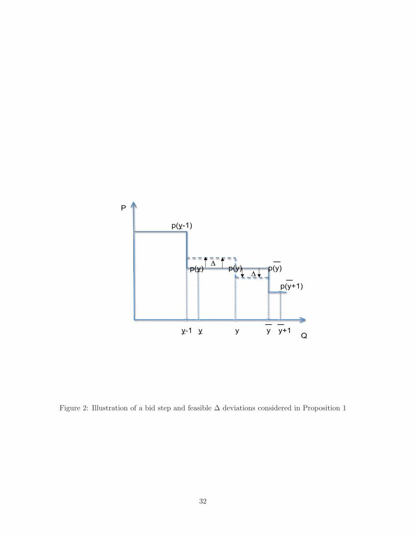
P
Qy-1 y y
p(y-1)
p(y)
y
p(y)!
!p(y)
y+1
p(y+1)
Figure 2: Illustration of a bid step and feasible ∆ deviations considered in Proposition 1
32

0 0.02 0.04 0.06 0.08 0.1 0.12 0.14 0.16 0.18 0.283.5
84
84.5
85
85.5
Quantity −− % of total supply
Pric
e
Residual supply faced by bidder 2
Residual supplyBidder 2
Figure 3: Illustration of the “resampling approach” (Section 3.1): bidder #2’s bid in auction #1, and
realizations of residual supply generated by resampling
Table 1: Summary statistics for 3-month T-bill auctions
Variable Average Std.dev. Min Max Total
Inflationa 67.8% 5.6% 58.0% 78.7%
No. of bidders 69 21.02 32 110 134b
Revenue (million $)c 456.3 443.1 31.4 1560.9 12369.1
Cover ratiod 28.9% 24.9% 0.2% 84.3%
Auction yielde 90.8% 6.9% 79.0% 101.4%
Variance of bidsf 0.035 0.031 0.005 0.134
aMonthly CPI from the Central Bank of TurkeybTotal number of unique bidders who participated in the auctions.cConverted using daily exchange rate datadQuantity sold/Quantity demandedeQuantity weighted average yield
fCalculated using the formula:PN
i=1(pi−pavg)2qiP
Ni=1
qi
33
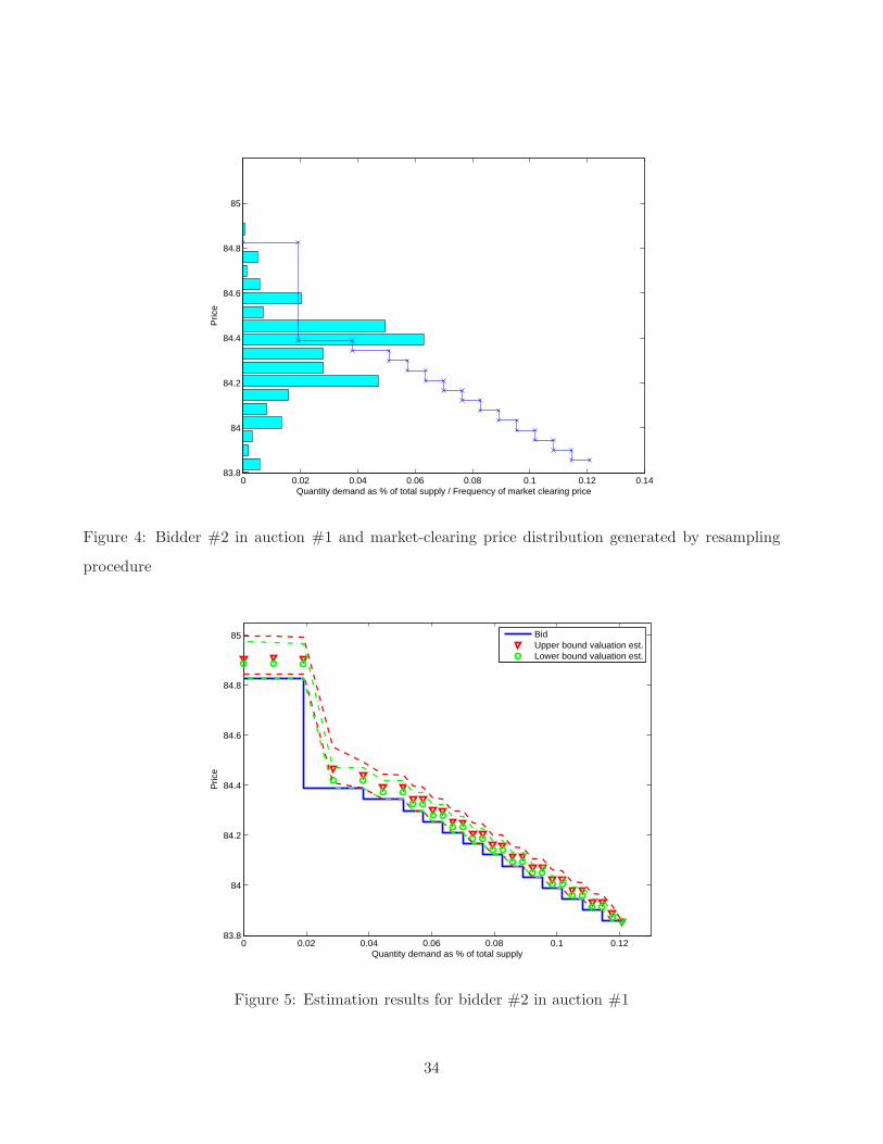
0 0.02 0.04 0.06 0.08 0.1 0.12 0.1483.8
84
84.2
84.4
84.6
84.8
85P
rice
Quantity demand as % of total supply / Frequency of market clearing price
Figure 4: Bidder #2 in auction #1 and market-clearing price distribution generated by resampling
procedure
0 0.02 0.04 0.06 0.08 0.1 0.1283.8
84
84.2
84.4
84.6
84.8
85
Quantity demand as % of total supply
Pric
e
BidUpper bound valuation est.Lower bound valuation est.
Figure 5: Estimation results for bidder #2 in auction #1
34

0 0.2 0.4 0.6 0.8 1 1.2 1.4 1.6 1.8 284
84.5
85
85.5
Quantity as % of total supply
Pric
e
Auction 1
Aggregate bid scheduleUpper bound marginal valuation estimateLower bound marginal valuation estimate
0 0.2 0.4 0.6 0.8 1 1.2 1.4 1.6 1.8 283.8
84
84.2
84.4
84.6
84.8
Quantity as % of total supply
Pric
e
Auction 12
Aggregate bid scheduleUpper bound marginal valuation estimateLower bound marginal valuation estimate
Figure 6: Counterfactual revenue comparison for auctions #1 and #12
35

Table 2: Counterfactual Ex Post Revenue and Efficiency Comparisons
UPATB revenue gain (upper bnd) UPATB revenue gain (lower bnd) UPATB efficiency gain
Auction 5th pc. Pt. est. 95th pc. 5th pc. Pt. est. 95th pc. 5th pc. Pt. est. 95th pc.
1 -0.35% -0.31% -0.26% -0.35% -0.33% -0.28% 0.00% 0.00% 0.00%
2 -0.08% -0.08% -0.05% -0.08% -0.08% -0.08% 0.00% 0.00% 0.00%
3 -0.31% 0.23% 0.53% -0.34% 0.17% 0.42% 0.00% 0.04% 0.05%
4 -0.15% -0.02% 0.09% -0.18% -0.07% 0.00% 0.00% 0.00% 0.01%
5 -0.06% -0.03% 0.03% -0.09% -0.06% -0.01% 0.00% 0.00% 0.01%
6 -0.02% 0.02% 0.06% -0.05% 0.00% 0.03% 0.00% 0.00% 0.00%
7 -0.13% -0.03% 0.03% -0.15% -0.06% 0.00% 0.00% 0.00% 0.01%
8 -0.10% -0.08% -0.03% -0.12% -0.10% -0.06% 0.00% 0.00% 0.00%
9 -0.22% -0.19% -0.14% -0.24% -0.21% -0.16% 0.00% 0.00% 0.00%
10 -0.16% -0.03% 0.11% -0.19% -0.06% 0.08% 0.00% 0.01% 0.01%
11 -0.13% 0.04% 0.21% -0.13% 0.01% 0.16% 0.00% 0.00% 0.00%
12 -0.07% 0.08% 0.25% -0.10% 0.05% 0.21% 0.00% 0.00% 0.00%
13 -0.06% 0.09% 0.13% -0.10% 0.05% 0.10% 0.00% 0.00% 0.00%
14 -0.02% 0.03% 0.13% -0.05% 0.00% 0.08% 0.00% 0.00% 0.00%
15 0.01% 0.11% 0.19% -0.04% 0.06% 0.15% 0.00% 0.00% 0.00%
16 -0.01% 0.05% 0.18% -0.04% 0.01% 0.15% 0.00% 0.00% 0.01%
17 -0.03% -0.02% 0.07% -0.06% -0.06% 0.03% 0.00% 0.00% 0.00%
18 -0.04% 0.42% 0.48% -0.08% 0.24% 0.36% 0.00% 0.04% 0.09%
19 -0.25% -0.17% -0.01% -0.30% -0.26% -0.20% 0.00% 0.00% 0.10%
20 0.06% 1.34% 1.12% -0.03% 0.41% 0.35% 0.02% 0.22% 0.26%
21 0.04% 0.31% 0.62% -0.06% 0.12% 0.34% 0.00% 0.00% 0.01%
22 -0.06% -0.03% 0.02% -0.09% -0.07% -0.03% 0.01% 0.01% 0.03%
23 0.03% 0.11% 0.13% -0.01% 0.03% 0.04% 0.00% 0.00% 0.00%
24 0.02% 0.11% 0.16% -0.02% 0.05% 0.10% 0.00% 0.00% 0.01%
25 0.01% 0.23% 0.24% -0.04% 0.12% 0.10% 0.00% 0.00% 0.01%
26 -0.01% 0.03% 0.29% -0.04% 0.00% 0.17% 0.00% 0.00% 0.01%
27 0.00% 0.47% 0.57% -0.14% 0.01% 0.03% 0.03% 0.10% 0.12%
Average -0.08% 0.10% 0.19% -0.12% 0.00% 0.08% 0.00% 0.02% 0.03%
36

Table 3: Counterfactual Ex Ante Revenue and Efficiency Comparisons
UPATB revenue gain (upper bnd) UPATB revenue gain (lower bnd) UPATB efficiency gain
5th pc. Pt. est. 95th pc. 5th pc. Pt. est. 95th pc. 5th pc. Pt. est. 95th pc.
-0.07% 0.12% 0.23% -0.11% 0.02% 0.11% 0.002% 0.020% 0.035%
37