Mechanics of Multi-Phase Frictional Visco-Plastic, Non ...cdn.intechweb.org/pdfs/28971.pdfMechanics of Multi-Phase Frictional Visco-Plastic, Non-Newtonian, Depositing Fluid Flow in

7

Mechanics of Multi-Phase Frictional Visco-Plastic, Non-Newtonian, Depositing

Fluid Flow in Pipes, Disks and Channels

Habib Alehossein CSIRO Earth Science and Resource Engineering, University of Queensland

Australia

1. Introduction

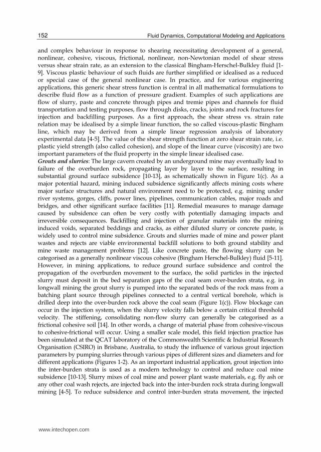
Background: Fresh concrete, fly ash and mining slurries are all frictional-visco-plastic fluids. Fresh concrete flow in Tremie pipes is used to control concrete flow rate and minimise bleeding and dilution when concrete is poured into deep submerged excavations for pile foundation construction. Slurries with very fine aggregates are used to backfill underground voids and mines to prevent subsidence and surface structural damage. Backfilling and injection of granular materials into mining induced voids, separated beddings and cracks, as either diluted slurry or concrete paste, is widely used to control subsidence. As a viable environmental solution, mine waste and rejected materials from underground coal seams are used in both backfilling and injection mine operations. For example, during longwall mining the grout slurry is pumped into the separated beds of the fractured rock mass through a pipeline connected to a central vertical borehole, which is drilled deep into the inter-burden rock strata above the coal mine seam. Either as dilute slurry or thick paste or cake, the fill material normally needs to travel a significant longitudinal distance either in a channel, a tremie pipe, a long pipeline, or radially in a disk shaped crack in the rock mass. An undesirable blockage can occur in the central borehole, in the crack or in the transportation channel or pipeline system when the slurry velocity falls below a certain critical threshold velocity, indicating a material phase change from cohesive-viscous to cohesive-frictional. This chapter presents complete analytical solutions of the required pump pressure versus fluid volume rate for such multi-phase fluids, which are categorised as frictional Bingham-Herschel-Bulkley fluids. The theory derived can be applied to flow of such fluids in pipes, disks and open channels. Furthermore, general analytical solutions have been developed for such fluids in terms of velocity and pressure gradients and velocity and pressure, as a function of flow length (e.g. pipe length, disk radial distance, or channel length) from which special and familiar equations for simpler fluids are derivable by mathematical reduction of the general equations. The formulation is distinct in considering many new aspects including: variable shear parameters rather than fixed values; inclusion of total nonlinear behaviour; and, implementation of a friction function to mimic behaviour of the depositing and consolidating stiff slurry or paste, which can cause a significant pressure rise as a result of the increased shear resistance. Bingham-Herschel-Bulkley fluids: Recent laboratory and field experiments on mine-backfill fluids, slurries, cements, pastes and concretes proved their wide range of shear resistance

www.intechopen.com

Fluid Dynamics, Computational Modeling and Applications 152

and complex behaviour in response to shearing necessitating development of a general, nonlinear, cohesive, viscous, frictional, nonlinear, non-Newtonian model of shear stress versus shear strain rate, as an extension to the classical Bingham-Herschel-Bulkley fluid [1-9]. Viscous plastic behaviour of such fluids are further simplified or idealised as a reduced or special case of the general nonlinear case. In practice, and for various engineering applications, this generic shear stress function is central in all mathematical formulations to describe fluid flow as a function of pressure gradient. Examples of such applications are flow of slurry, paste and concrete through pipes and tremie pipes and channels for fluid transportation and testing purposes, flow through disks, cracks, joints and rock fractures for injection and backfilling purposes. As a first approach, the shear stress vs. strain rate relation may be idealised by a simple linear function, the so called viscous-plastic Bingham line, which may be derived from a simple linear regression analysis of laboratory experimental data [4-5]. The value of the shear strength function at zero shear strain rate, i.e. plastic yield strength (also called cohesion), and slope of the linear curve (viscosity) are two important parameters of the fluid property in the simple linear idealised case. Grouts and slurries: The large cavern created by an underground mine may eventually lead to failure of the overburden rock, propagating layer by layer to the surface, resulting in substantial ground surface subsidence [10-13], as schematically shown in Figure 1(c). As a major potential hazard, mining induced subsidence significantly affects mining costs where major surface structures and natural environment need to be protected, e.g. mining under river systems, gorges, cliffs, power lines, pipelines, communication cables, major roads and bridges, and other significant surface facilities [11]. Remedial measures to manage damage caused by subsidence can often be very costly with potentially damaging impacts and irreversible consequences. Backfilling and injection of granular materials into the mining induced voids, separated beddings and cracks, as either diluted slurry or concrete paste, is widely used to control mine subsidence. Grouts and slurries made of mine and power plant wastes and rejects are viable environmental backfill solutions to both ground stability and mine waste management problems [12]. Like concrete paste, the flowing slurry can be categorised as a generally nonlinear viscous cohesive (Bingham Herschel-Bulkley) fluid [5-11]. However, in mining applications, to reduce ground surface subsidence and control the propagation of the overburden movement to the surface, the solid particles in the injected slurry must deposit in the bed separation gaps of the coal seam over-burden strata, e.g. in longwall mining the grout slurry is pumped into the separated beds of the rock mass from a batching plant source through pipelines connected to a central vertical borehole, which is drilled deep into the over-burden rock above the coal seam (Figure 1(c)). Flow blockage can occur in the injection system, when the slurry velocity falls below a certain critical threshold velocity. The stiffening, consolidating non-flow slurry can generally be categorised as a frictional cohesive soil [14]. In other words, a change of material phase from cohesive-viscous to cohesive-frictional will occur. Using a smaller scale model, this field injection practice has been simulated at the QCAT laboratory of the Commonwealth Scientific & Industrial Research Organisation (CSIRO) in Brisbane, Australia, to study the influence of various grout injection parameters by pumping slurries through various pipes of different sizes and diameters and for different applications (Figures 1-2). As an important industrial application, grout injection into the inter-burden strata is used as a modern technology to control and reduce coal mine subsidence [10-13]. Slurry mixes of coal mine and power plant waste materials, e.g. fly ash or any other coal wash rejects, are injected back into the inter-burden rock strata during longwall mining [4-5]. To reduce subsidence and control inter-burden strata movement, the injected

www.intechopen.com

Mechanics of Multi-Phase Frictional Visco-Plastic, Non-Newtonian, Depositing Fluid Flow in Pipes, Disks and Channels 153

slurry solid particles must deposit in the opened strata bed separation gaps or cracks before crack closure [10-13]. The mechanics of non-Newtonian fluids flowing between parallel disks is a classical fluid mechanics problem that has been studied by a number of researchers in the past for their specific problems of interest [3-4].

(a) Concrete flow testing (b) Concrete tremie pipe flow (c) Slurry flow in pipe and strata

Fig. 1. Various applications of viscous slurry and paste fluids: (a) channel flow for workability and consistency testing of concrete; (b) Concrete termie pipe flow into submerged foundations; (c) multi-phase slurry flow in pipes and fractured rock strata for void backfilling.

Concrete: Fresh concrete flow through Tremie pipes is used to control concrete flow rate and minimise segregation, bleeding and dilution when poured or placed into deep submerged excavations for pile foundation construction. Slurries with very fine aggregates are used to backfill underground voids and mines to prevent subsidence and surface structural damage. Backfilling and injection of granular materials into the mining induced voids, separated beddings and cracks, as either diluted slurry or concrete paste, is widely used to control coal mine subsidence. As a viable environmental solution, mine waste and rejected materials from underground coal seams in the form of either cementitious or non-cementatious grout, are used in both backfilling and injection mine operations. For example, during longwall mining the grout slurry is pumped into the separated beds of the rock mass through a central vertical borehole, which is drilled deep into the inter-burden rock strata above the coal seam. Either as dilute slurry or thick paste or cake, the fill material normally needs to travel a significant distance in either a long pipeline, or radially in a disk type crack formation of the rock mass. An undesirable blockage can occur in the central borehole, in the disk gap or in the transportation channel or pipeline system, when the slurry velocity falls below a certain critical threshold velocity, indicating a material phase change from cohesive-viscous to cohesive-frictional. Indirect index measure of concrete viscosity and plastic yield is made via an L-box channel measuring workability and flowability of tremie pipe concrete. The L-box test, originally developed for super-workable concrete [6-9] is a relatively newly introduced concrete test to measure the consistency, workability and flowability of a tremie pipe concrete, hence, it is indirectly related to concrete plastic yield and viscosity [6]. Concrete is poured in the rectangular vertical chimney part of the L-box and is allowed to flow in the horizontal channel part, once a sliding gate is opened. The time and profile of the concrete flow in the horizontal channel is measured to compare viscous-plastic behaviour of different concretes. The variation of flow velocity with time and position from the time the sliding gate is opened until the flow reaches static equilibrium has been simulated and formulated by a representative dimensionless partial differential equation (PDE). Mathematically, the resulting equation is of the same form as a non-homogeneous heat-conduction equation [6].

y2 y1

h Concrete

L0 L w

y

x u(t,x)

Concrete c = Cw

D

Water level

Ho/C

He

Hf

Tremie pipe

Lt

Hw

Pressure balance point o

w)

Hb

Slurry casing

s)

Hs

Slurry level

Extracted underground coal seam

Total surface ground subsidence

Bed separation gap Injection borehole

Pump

Batch

Plant Pipeline

www.intechopen.com


In this chapter complete analytical solutions of the required pump pressure versus fluid volume rate are discussed for such multi-phase fluids, which are categorised as frictional Bingham-Herschel-Bulkley fluids. The discussed theory can be applied to flow of such fluids in pipes, disks and open channels. Furthermore, general analytical solutions have been developed for complex fluids in terms of velocity and pressure gradients and velocity and pressure, as a function of flow length (e.g. pipe length, disk radial distance, or channel length) from which special and familiar equations for simpler fluids are derivable by mathematical reduction of the general equations. The formulation is distinct in considering many new aspects including: variable shear parameters rather than fixed values; inclusion of total nonlinear behaviour; and, implementation of a friction function to mimic behaviour of the depositing and consolidating stiff slurry or paste, which can cause a significant pressure rise as a result of the increased shear resistance.

2. Frictional Bingham-Herschel-Bulkley fluid

The general constitutive equation, relating fluid shear stress to shear rate for such general nonlinear, non-Newtonian, viscous, plastic, frictional fluids, which can be applied to fresh concrete, mine backfill slurries and high frictional multiphase fluids, is as follows [4-9]

n

(t, ) (t, )(t, ) ┤(t, ) ┟(t, ) (t, ) ξ(t, )p(t, )

ˆ ˆ

0

u x u xτ x x x τ x x xx x

(1)

In Equation (1) is shear stress tensor, u is velocity vector, and are linear and

nonlinear viscosities, 0 is plastic yield, p is pipe pressure and is concrete friction

coefficient. The last term, involving the friction and pressure terms (p), is a frictional

resistance term which can be applied only when a pipe blockage occurs due to the

concrete granular material friction and needs to be reopened by a higher pressure flow,

otherwise it can be ignored [4-9]. See Figure 2 for a visual definition of the different shear

terms and parameters involved in Equation (1).

Fig. 2. Schematic diagrams showing various shear stress components in Equation (1). 0 is

the constant uniform plastic yield component, with no viscosity; is the Newtonian linear

viscosity coefficient of the linear velocity gradient y with a wall value yh.; is the non-linear

viscosity; is the friction coefficient of the fluid pressure p.

x

p yh ynh

Pipe flow direction

Q

Shear resistance components

www.intechopen.com


Fig. 3. Shear stress vs shear rate (range 0-700/s) for a sample at solid weight concentration range 30%-60%. Numbers in legend table show Bingham plastic linear fit model to these results in the range of 0-100/s. For instance, for 50% solid concentration in the shear rate range of 0-100/s of the sample, the linear viscosity (Bingham slope) is 0.0106 Pa.s and the yield (Bingham intercept) is 1.6432 Pa.

We can measure these parameters by a viscometer-testing device [4-5]. Sometimes for slurries

of various solid particle concentrations, the viscometer test results can conveniently fit into one

or two linear models (Bingham plastic) for the whole range of shear strain rate. Figure 3 shows

examples of multi-linear or bilinear model for slurries of different concentrations for two

distinct range of shear strain rate 0-100 /s and 100-700 /s. The Bingham models can be

identified by its two main parameters (yield intercept and viscosity slope.

3. Governing equations

Governing equations of most fluid mechanics problems normally start with the general

basic Reynolds transport theorem of continuum mechanics [15]. This is initially an integral

relation stating that the sum of the changes of any intensive fluid property, such as mass,

momentum and energy, defined over a control volume CV, denoted here by symbol , must

be equal to what is gained or lost through the boundaries of the volume, or control surface

(CS), plus what is created or consumed by sources and sinks inside the control volume [15].

CV CS CV

ddV . dA QdV 0

dt u n

(2)

In Equation (2), u

is fluid velocity vector, n

is normal vector to the control surface dA, and

Q is the fluid source or sink. Using integration by parts, the second integral can also be

0

10

20

30

40

50

0 100 200 300 400 500 600 700

Shear rate (1/s)

Sh

ea

r s

tre

ss

(P

a)

Weight solid concentration (%) = C

Viscosity (Pa.s) = Plastic yield (Pa) =

C = 60 %

= 0.0499

= 10.346

C = 50 %

= 0.0106

= 1.6432

C = 40 %

= 0.005

= 0.1967

C = 30 %

= 0.0051

= 0.0187

www.intechopen.com


transformed to a volume integral by the divergence theorem. Since the whole grouped volume integral must be zero for any arbitrary control volume CV, it implies that the integrand itself must be zero. Therefore, our theory can be started with the following general basic differential equation:

d┪

.┪ Q 0dt

u

(3)

Applying the general conservation Equation (3) to mass and momentum, the Navier- Stokes isothermal equations of continuity and momentum [15] are recovered:

.┩ ┩ 0 u

(4)

D

. ┩ ┩Dt

uσ g

(5)

where x i i/ e

is the gradient vector, is the fluid density, σ

is the stress tensor and g

is the body acceleration or gravity vector. The stress tensor depends on a mean fluid normal stress or pressure ( 1

jj iip ├ ┫ ) and a deviator stress representing shear stresses ij, which depends on fluid viscosity and velocity gradients.

ij ij ij┫ p├ ┬ (6)

As shown by [3-4], the deviatoric shear stress in (6) for cohesive, frictional, viscous, non-Newtonian slurries depends not only on fluid velocity gradients and yield plastic shear strength, but also on fluid pressure causing frictional resistance to flow, particularly during a blockage (Q →0). As discussed earlier in Equation (1), on the basis of several laboratory experiments on soil like slurries, a general shear stress versus shear strain constitutive material law is proposed for viscous, cohesive, frictional, plastic slurries in which the fluid shear stress is a nonlinear function of shear rate and longitudinal distance. Equation (1) has the following general form when written tensor notation is applied:

n

ij i,j j,i i,j j,i 0ij ij┬ ┤ u u ┟ u u ┬ ξp├ (7)

As discussed earlier and also shown in Figure 2, the first term on the right hand side is the familiar linear Newtonian component, the second term is the nonlinear pseudo-plastic component, the third term is the yield component and the forth term is the pressure component, in which is a coefficient of granular material friction which is the same tangent function of the material friction angle [14]. In the theoretical analysis discussed here, it is assumed that: 1. the flow is laminar and the fluid is incompressible, steady state, stationary, and

isothermal and axisymmetric with no eddies and no gravity effects; 2. axially symmetric condition implies that the radial flow component (in a pipe) and

circumferential flow (in a disk) must vanish. In other words ux2 = ux3 = 0;

3. when there is a full blockage (Q = 0), the friction term p is a dominant term; 4. the classical term “fluid” has loosely been used interchangeably with “slurry”; to refer

to a “slurry”, whenever an equivalent “fluid” model can represent the overall, average, mechanical behaviour of the “slurry”.

www.intechopen.com


We now introduce a new set of independent variables to represent coordinate axes of both

radial disk and pipe flow systems, namely: x1 axis is always in the direction of the main flow

direction, i.e. either radial disk flow, or longitudinal pipe or channel flow, x2 is the axis

normal to the flow direction in the flow cross-section plane, and x3 is the hoop or

circumferential axis direction identical to hoop angle .

4. Reduced one dimensional equations

Consider now the simple problem of fluid flow through either (i) a uniform circular pipe of

inside diameter 2h, as shown in Figure 4 (left), or (ii) a radial disk of thickness 2h, as in

Figure 4 (right), or (iii) a channel, as part of an L-Box testing device shown in Figure 1 (a).

Fig. 4. Non-Newtonian viscous-plastic flow in a pipe (left) and in a radial disk (right) with fluid flow parameters

Fluid flow through a pipe of uniform, circular, cross-section is known as the Hagen–

Poiseuille flow problem [5]. It is assumed that the circular pipe flow is symmetric around

the pipe longitudinal x-axis, the normal stresses are simply the fluid pressure, p, the fluid is

incompressible and non-Newtonian in a steady state condition, there is no velocity

component in the pipe circular cross-sectional plane, i.e. the plane normal to the pipe length

direction. Similarly, it is assumed that the flow in a disk is also non-Newtonian, steady state,

incompressible and laminar and the radial disk flow is also cylindrically axi-symmetric [4].

Hence, implementing all these assumptions implies that in all flow cases both normal to

flow velocity components (u2, u3) are zero and there is no variation in velocity or pressure

with time. In other words, we have

1 1 2u u u(x ,x ) (8)

2 3 ┠u u u 0 (9)

i i i 2 2u / t u / ┠ p/ t p/ ┠ u / x p/ x 0 (10)

We now define two separate flow gradient functions [4-5], (a) gradient with respect to x1

and (b) gradient with respect to x2, viz.

1

2

uy

x

(11a)

x1

x2

2h x2

Slurry x1x1x1x1n

Q

u(x1, x2) x1 h

h

Q, xxxxn

x1

u1

Q

x1

r

y

2h h u1(x1, x2) x1

x2

h

www.intechopen.com


1 1x u (11b)

11 1

2

uψ x x 'x

y (11c)

Hence, the general, basic equations of continuity (4) and momentum (5) reduce to Equations (12) for pipe flow and (13a,b) for radial flow.

PF (Pipe flow): 2

2 2 1

x ┬1 p

x x x

(12)

RF (Radial Flow): 2

1 1 2

1 u0

x x x

(13a)

1 2

p ┬0

x x

(13b)

It should be noticed that gravity effect can be incorporated into the pressure gradient term

in pipe flow Equation (12), where is the fluid unit weight and is the inclination angle of

the pipe with respect to horizontal axis. In order to consider gravity in a pipe flow, p

x

in

(12) should be replaced with p ┛sin(┚)x

, as suggested in [2]. The shear stress 1 2┬(x ,x ) in

(12) and (13) is a 2D version of the general case shown in (7), which is reproduced in

Equation (14) below [4-5].

n

1 2 1 1 1 1 1┬(x ,x ) ┤(x )y ┟(r)y ┬ (x ) ξ(x )p(x ) (14)

No slip boundary conditions, i.e. no velocity at the pipe or disk walls, and a full axial or

radial symmetry of the flow are assumed. Hence, Equations (11-13) must be solved subject

to the following boundary conditions:

1 2u u u(x h) 0 (15a)

22

u(x 0) 0

x

(15b)

Substituting (14) in (12) and (13) and integrating over x2, will give us the following pressure-

gradient equations

PF: n21 1 2 1 2 0 1 1 1

1

x dp(x ) ┬ ┤(x )y(x ) ┟(x )y (x ) ┬ (x ) ξ(x )p(x )

2 dx (16)

RF: 2 1 11

dpx (x ) ┤(x )y ┟(r)y

dxn (17)

www.intechopen.com


The pressure gradient Equations (16) and (17) must be satisfied at all points, including the

boundary point, h. Therefore, at the wall boundary point (x2=h) we have

PF: n1 h 1 h 1 h 0 1 1 1 h

1

h dp(x ) ┬ ┤(x )y ┟(x )y ┬ (x ) ξ(x )p(x ) F(y )

2 dx (18)

RF: 1 h 1 h h 1 h1 1 1

dp 1 1h ┤(x ) ψ ┟(x ) ψ f(ψ /x ) f(y )

dx x x

n (19)

where yh, h and h are the boundary values of y, and , i.e. at the point x2 = h. In other words,

PF: 2h 2 x h

2

uy y(x h)

x

, h 2┬ ┬(x h) , h 2ψ ψ(x h) (20)

If yh in (18), or h in (19), are known, the pipe pressure p can be calculated by integrating

these equations directly. The result can still be in integral forms depending on the

complexity of the coefficient functions such as: viscosity x or x, plasticity, x or

friction x

PF: 1

0

x

h 1 1

2p ┬ (x )dx

hx

(21a)

RF: 1

0

x

h 1 1

x

1p f(ψ /x )dx

h (21b)

For example, the pipe pressure can be written in a general integral form (Equation (22)) in

terms of the integral coefficients A1, B1, C1 [5].

n 10 0 1 h 1 h 1p p v A y B y C v (22)

In Equation (22), v(x1) is an exponential function of x1 and h and A1, B1, C1 are integral

coefficients similar to those produced for radial flow [4], viz.

2

ξdxhv(x) e

(23)

0

x

1

x

2A v(x)┤(x)dx

h (24a)

0

x

1

x

2B v(x)┟(x)dx

h (24b)

www.intechopen.com


0

x

1 0

x

2C v(x)┬ (x)dx

h (24c)

As shown in [4-5], evaluations of these integrals become straight forward and generic, if we

first find the normalised forms of the dimensional functions, (x), (x), (x) and (x) in the

shear stress Equations (16) and (17). Using the same symbols, but in Italic fonts, let the italic

symbols , , and be the normalised counterparts of (x), (x), (x) and (x),

respectively. As discussed in detail in [4-5], all the four functions , , , , can be

represented by one symbolic generic function, , i.e. (0, s, r, n). The normalised form of

is simply

( ) 1 ( 1)nsr r (25)

in which s is the normalised slope and n is the general power factor for any nonlinear

behaviour. In other words,

0

┙┙

,0 0

┙ r1 1

┙ r

n

s

(26)

Therefore, the integrals (24) have the following general non-dimensional form which can be

integrated numerically [4-5]:

PF: 1 1

( )x x

k dxI x v(x) (x)dx e (x)dx

(27a)

RF: 111 1

1 1

1( ) [1 ( 1) ] 1 1

1 1

x xnn nnn n ns

s

xI x x x dx x x n x x dx

n n (27b)

However, for constant properties of slurry, the A1, B1, C1 parameters reduce to either a

simple exponential function of x=x1, in the presence of a friction coefficient, i.e. ≠0, or a

simple linear function in terms of pipe length (L = x-x0), in the absence of friction coefficient,

i.e. =0. In other words, the values of these coefficients, as described by the integrals (24),

can be calculated from relations (28) for the case where = = 0 = constant, but =0, and

from relations (29) for the case where = = 0 = constant, but ≠0.

1 1

1 0A 2h ┤(x-x ) 2h ┤L , 11B 2h ┟L , 1

1 0C 2h ┬ L (28)

1 L

┤A v

ξ , 1 L

┟B v

ξ , 0

1 L

┬C v

ξ ,

2 ξLh

Lv e (29)

Figures 5 and 6 show some typical values of the function I for a range of viscosity and

plasticity parameters in a radial flow, namely n from (0) to (2), n from (0) to (2), s from (0)

to (2) and normalised r=x from (1) to (100) [4].

www.intechopen.com


Fig. 5. Values of integral function I with radial distance r for some values of parameters n,

n and s, as indicated in Equation (27b)

Fig. 6. Values of integral function I with radial distance r for some values of parameters n,

n and s, as indicated in Equation (27b)

I(r , n , n , s)

0

5

10

15

20

25

0 20 40 60 80 100

Normalised radial distance r

No

rma

lis

ed

in

teg

ral I

(r,

n, n,

s)I(r,0,0,0)

I(r,0,0,0.5)

I(r,0.5,0,0)

I(r,0.5,0,0.5)

I(r,1,0,0)

I(r,1,0,0.5)

I(r,1.5,0,0)

I(r,2,0,0)

I(r,1.5,0,0.5)

I(r,2,0,0.5)

10

100

1000

10000

100000

1000000

0 20 40 60 80 100

Normalised radial distance r

I(r

, n

, n,

s)

I(r ,0.0 ,2.0 ,1.0)

I(r ,0.0 ,2.0 ,0.5)

I(r ,0.5 ,2.0 ,1.0)

I(r ,0.5 ,2.0 ,0.5)

I(r ,0.0 ,1.0 ,1.0)

I(r ,0.5 ,1.5 ,0.5)

www.intechopen.com


5. Solutions for pipe and radial flow

The pressure gradient dependency in all Equations (16)-(17) can be removed by dividing

general functions or Equations (16)-(17) to their corresponding boundary values, i.e.

Equations (18)-(19). Thus, we have a ratio of two polynomial functions, with a numerator

that is a function of y, and a denominator that is a function of yh, as shown in Equation (30a,

b), in which a, b, A, B, C are functions of flow line distance x1 only.

PF:

h

n

2 nh h hh

Ay By C F(y)┬ Fx h h h h

┬ F(y ) FAy By C

(30a)

RF: h

n

2 nh h hh

ay by f(y)┬ fx h h h h

┬ f(y ) fay by

(30b)

To solve (30a) or (30b) for our primary unknowns, either y or , we need another equation

in terms of the flow rate, Q, which must be conserved at any section normal to x1 direction.

The results are integral equations relating velocity gradient y, or yh (or , or h in the case of

radial flow) to the flow rate Q [4-5].

PF: h3 3

2 1 2 h h h

A 0

┨Q u.dA 2┨ x u dx h y F G

3

(31a)

RF: h2 2

2 1 2 h h h

A 0

Q u.dA 2┨ x u dx 2┨h ψ f g (31b)

Values of velocity gradient at the wall boundary, yh, or the function h= x1 yh, needs be

calculated generally by the Newton-Raphson iteration [16]. Hence solutions to (31) take the

following general forms:

PF: i

i 1 i

h h h hh h

h h h

(Q y )G'(y ) G(y )y y

(Q y )G''(y ) , h 3

3Q Q

┨h (32a)

RF: i

i 1 i

h h h hh h

h h h

(Q ψ )g'(ψ ) g(ψ )ψ ψ

(Q ψ )g''(ψ ) , h 2

1Q Q

2 h (32b)

In Equation (31)-(32) f, F, g and G are polynomial functions of the unknown variable y or .

2 22 3 2n 1 n 2a b 2ab

g ψ f dψ ψ ψ ψ3 2n 1 n 2

(33a)

2 2 2 2 2n n 1g' ψ f ψ a ψ b ψ 2abψ (33b)

2 2 2n 1 ng'' ψ 2a ψ 2nb ψ 2(n 1)abψ (33c)

www.intechopen.com


nf ψ aψ bψ (33d)

n 1f' ψ a nbx (33e)

3 23 4 2 3 2 3

3 2 23n 1 2n 2 2n 1

2 2n 3 n 2 n 1

A 3ACG(y) F dy y A Cy y C y

4 2

B 3AB 3B Cy y y

3n 1 2n 2 2n 1

3A B 6ABC 3BCy y y

n 3 n 2 n 1

(34a)

3 3 3 2 2 2 3 3 3n 2 2n 1

2 2n 2 n 2 n 1 2 n

G'(y) F A y 3A Cy 3AC y C B y 3AB y

+3B Cy 3A By 6ABCy 3BC y

(34b)

3 2 2 2 3 3n-1 2 2n

2 2n-1 2 n 1 n 2 n-1

G''(y) 3A y 6A Cy 3AC 3nB y 3(2n 1)AB y

6nB Cy 3(n 2)A By 6(n 1)ABCy 3nBC y

(34c)

nF(y) ┬ Ay By C (34d)

n 1F'(y) A nBy (34e)

Determination of other parameters is rather straight forward. Once, yh or h are determined,

the wall shear stress, radial pressure gradient and pressure functions can be determined

directly from Equations (16)-(19). For instance, we can calculate the fluid velocity by direct

integration of the velocity gradient.

PF: 2x 2 n 1

2 22 h0

(n 1)Ay 2nByuu(x ) u(0) dx u(0) h

x 2(n 1)F(y )

(35a)

RF: 2x 2 n 1

2 22 2 h0

u (n 1)aψ 2nbψu(x ) u(0) dx u(0)

x 2(n 1)x f(ψ )

(35b)

where u(0) is the maximum velocity at the flow centre line given by

PF:

2 n 1h h

0 maxh

(n 1)Ay 2nByu(0) u u h

2(n 1)F

(36a)

RF: 2 n 1h h

0 max2 h

(n 1)aψ 2nbψu(0) u u h

2(n 1)x f

(36b)

www.intechopen.com


Hence, the velocity profile across the flow cross-section is given by

PF:

2 n 1

max 2 n 1h h

(n 1)Ay 2nByu u 1

(n 1)Ay 2nBy

(37a)

RF: 2 n 1

max 2 n 1h h

(n 1)aψ 2nbψu u 1

(n 1)aψ 2nbψ

(37b)

The average flow velocity can also be determined in the usual manner by integrating (36) directly, namely

h

2 2 2 max 0h02 20

1u u(x )x dx u 1 ┣

x dx (38)

Where 0 is a function of yh, or h (in the case of radial flow [4]).

PF: 2

h h h h0 0 h

2 n 1h h

y F G F┣ G (y ) 13 3n

Ay By2 n 1

(39a)

RF:

2(n 1)1 n 1 2 21 h 2 h

0 0 h 2(n 1)1 n 1 2 23 h 4 h

1 n a bψ n a b ψ┣ g (x )

3 n a bψ n a b ψ

(39b)

In Equation (39b) ni is a constant depending only on the power factor n, given by

1

3n(n 3)n

(n 1)(n 2)

, 2

2

6nn

(n 1)(2n 1) ,

3

(3n 1)n 3

(n 1)

, 4

6nn

(n 1) (39c)

All the above solutions (e.g. Equations (32)) are also reducible to the classical solutions. For example, the average flow velocity becomes half of the maximum flow velocity for pipe flow, and 2/3 of the maximum flow velocity in the case of radial flow, for the case of pure Newtonian fluid [4-5].

Slurry flow may be assumed to stop in the case of a blockage (Q 0), which means the values of yh and g(yh) are identically zero. This is due to the effects of the cohesive

frictional terms ( and 0) introduced in the shear stress Equations (16-17), which now become dominant in blocking the slurry flow. In the slurry industry, a critical question always arises on what the minimum pump pressure is required for a given slurry flow rate either to transport it to a given distance, or be able to reopen a blockage in a specified pipe length. The minimum required pump pressure can be calculated from Equation (21), which depends on the wall shear resistance in the pipeline or the disk. The wall shear stress is a function of the longitudinal distance x and velocity gradient yh. Practically, during the field slurry injection, the minimum required pump pressure to transport the slurry to a given distance is one of the most important questions that needs to be addressed [4-5].

www.intechopen.com


6. Tremie pipe concrete flow

The flow theory developed for general viscous-plastic-frictional fluids can be applied to fresh wet concrete pastes and slurries as well. Again, an important question would be the relation between the flow rate, Q, and the pressure, p. Similar to the pipe flow discussed above, we may assume a fully developed laminar, one dimensional flow, where x2 is the radial distance from the tremie pipe’s axis of symmetry (Figure 1, middle) [6-9]. Gravity plays a major role as the main driving force for concrete flow in tremie pipes, thus, it cannot be ignored. Therefore, equation (12) becomes

22 c

2 1

(x ┬) px ┛ sin(┠)

x x

(40)

It is assumed that the tremie pipe generally makes an angle with the horizontal x axis, where = 90 indicates a vertical tremie. In Equation (40), x2 is the coordinate radius or radial distance from the pipe’s cross-sectional centre, p is pressure and c is the effective concrete unit weight. As a special case, a specific analytical solution from the general solution (32a) can be derived for a linear Bingham-plastic model [5]. In this particular solution, the tremie pipe flow rate, Q, becomes a 4th order polynomial function of the tremie pipe diameter, D. Furthermore, the flow rate is inversely proportional to the viscosity, 0and (partially) proportional to the differential pressure at the two ends of the tremie pipe [6], p, of length Lt. In other words we have:

4 3

c 0t

┨D Δp ┨DQ ┛ sin ┠ ┬

128┤ L 24┤ (41)

The pressure differential between the two ends of the tremie, p, can in theory accept any arbitrary value; from negative to zero and positive numbers. In the case of a zero p, the driving pressure is simply the gravity term containing the concrete unit weight, cand inclination angle . 7. Concrete flow in a rectangular channel

Concrete flow during pouring and flowing in channels, chutes and testing equipment for testing purposes are normally not at a steady state situation [6]. General time-dependent 2D and 3D differential equations governing flow of concrete in rectangular channels and chutes can be developed and solved numerically, as shown in [6]. However, for the sake of understanding, it is also possible to reduce these equations to a simple 1D form, based on an assumption that there is no significant independent variation in any variable or function in the normal directions x2 and x3 compared to the longitudinal main flow direction x1. In other words,

2 1,x 1 ,x 1 ,t 1┬ (t,x ) p (t,x ) ┩u (t,x ) 0 (42)

which gives a solution in terms of Fourier coefficients [6]

2 2

0

( , ) cos( ) sin( )na tn n n n

n

u t x e A x B x mx

(43)

www.intechopen.com


In the solution (43) is an arbitrary constant satisfying both the differential equation and the

boundary conditions, while An and Bn are Fourier coefficients to be determined from the

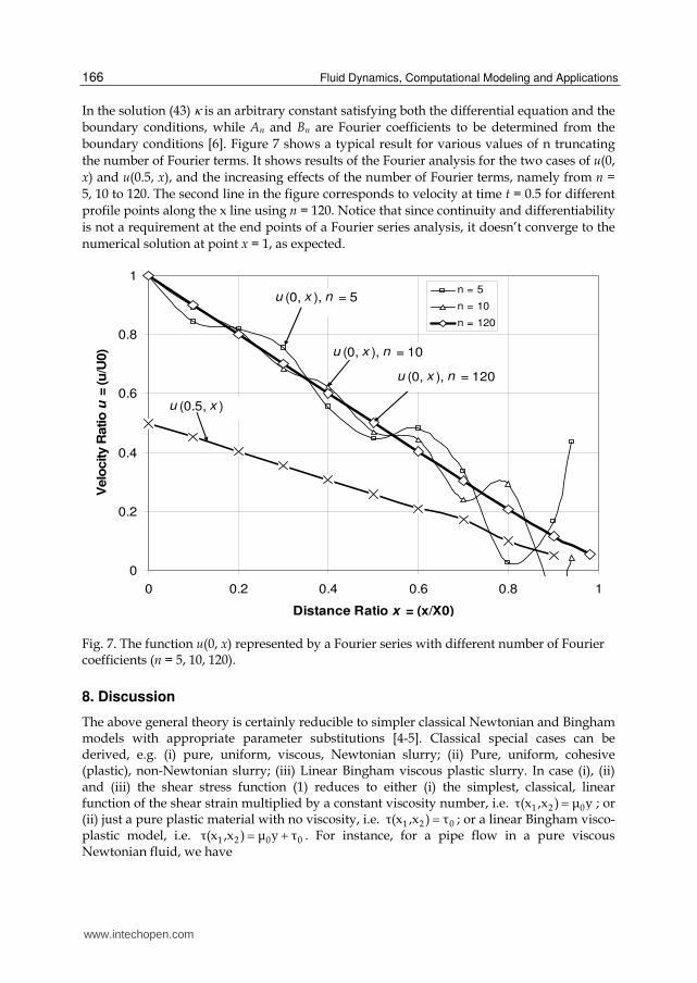
boundary conditions [6]. Figure 7 shows a typical result for various values of n truncating

the number of Fourier terms. It shows results of the Fourier analysis for the two cases of u(0,

x) and u(0.5, x), and the increasing effects of the number of Fourier terms, namely from n =

5, 10 to 120. The second line in the figure corresponds to velocity at time t = 0.5 for different

profile points along the x line using n = 120. Notice that since continuity and differentiability

is not a requirement at the end points of a Fourier series analysis, it doesn’t converge to the

numerical solution at point x = 1, as expected.

Fig. 7. The function u(0, x) represented by a Fourier series with different number of Fourier coefficients (n = 5, 10, 120).

8. Discussion

The above general theory is certainly reducible to simpler classical Newtonian and Bingham models with appropriate parameter substitutions [4-5]. Classical special cases can be derived, e.g. (i) pure, uniform, viscous, Newtonian slurry; (ii) Pure, uniform, cohesive (plastic), non-Newtonian slurry; (iii) Linear Bingham viscous plastic slurry. In case (i), (ii) and (iii) the shear stress function (1) reduces to either (i) the simplest, classical, linear function of the shear strain multiplied by a constant viscosity number, i.e. 1 2 0┬(x ,x ) ┤ y ; or (ii) just a pure plastic material with no viscosity, i.e. 1 2 0┬(x ,x ) ┬ ; or a linear Bingham visco-plastic model, i.e. 1 2 0 0┬(x ,x ) ┤ y ┬ . For instance, for a pipe flow in a pure viscous Newtonian fluid, we have

0

0.2

0.4

0.6

0.8

1

0 0.2 0.4 0.6 0.8 1

Distance Ratio x = (x/X0)

Velo

city R

atio

u =

(u

/U0)

n = 5

n = 10

n = 120

u (0, x ), n = 5

u (0, x ), n = 10

u (0, x ), n = 120

u (0.5, x )

www.intechopen.com


rx

u(r,x)┬ (r,x) ┤(x) ┤yr

, 0┤(r) ┤ , ┟ ┬ ξ n 0 (44a)

Substituting these values in equations (16-32), we recover the well-known Newtonian

solutions [15], as expected. It can be seen that for this case the function 0 h

1g (y )

2

confirming the classical result, maxr r

1u (r) u

2 . Furthermore, we have:

3

40h h

┤g y

4 (44b)

0

1g

2 (44c)

h 3

4Qy

┨h (44d)

0hx 3

4┤ Q┬┨h

(44e)

04

8┤ Qdp

dx ┨h (44f)

00 4

8┤ Qp p L

┨ h (44g)

max 2

2Qu(0,x) u

┨h (44h)

2 2

max max2 2h

y ru(r,x) u 1 u 1

y h

(44i)

max 0 max

1u u 1 g u

2 (44j)

Figure 8 shows velocity profiles in normalised form for the “three special cases” discussed

above. For the general Bingham fluid with constant non-zero values of 0 and 0, the pipe

velocity profile follows a parabolic curve close to the special pure viscous case (i), when

fluid viscosity is dominant or the ratio 0/0 is small, and moves towards the uniform

profile of the special case (ii), when plastic yield or cohesion is dominant or the ratio 0/0 is

large, as shown in the figure. Figure 9 demonstrates an example of a Bingham plastic

solution for radial disk flow, where the contribution of each of the two shear parameters is

separately demonstrated.

www.intechopen.com


Fig. 8. Comparisons of normalised velocity profiles for different slurries of various viscosity

() and plasticity () in a pipe flow

Fig. 9. Contribution of viscosity and cohesion to pressure drop for a Bingham plastic slurry in a radial disk flow

0

0.2

0.4

0.6

0.8

1

0 0.2 0.4 0.6 0.8 1

Pipe radial distance (r/h)

Pip

e v

elo

cit

y (

u/u

max)

Case (i), pure viscous

Case (ii), pure plastic

(iii),

(iv),

(v),

(vi),

0

20

40

60

80

100

0 100 200 300 400 500

Disc radial flow distance (radius), r (mm)

Pre

ss

ure

, p

0-p

(P

a)

= 0.008 Pa.s

0 = 0.3 Pa

0 = 0.3 Pa

= 0.008 Pa.s

h=4mm

Q = 20 lit/hr

r0 = 2mm

0

30r

rln

πh

μQ6pp

www.intechopen.com


As a numerical pipe flow example, consider a slurry modelled by a linear Bingham plastic model, where 0 = 0.1Pa.s and 0 = 0.1Pa. As shown in Table 1, the maximum and average velocities in the pipe are 3.54 m/s and 1.76 m/s, respectively. The table also shows a list of values for several other variables and parameters used in the present theory.

Table 1. Numerical example for cohesive-viscous slurry ( = 0.1 Pa.s, = 0.1)

Slurry behaviour is controlled by its two distinct material components, i.e. the solid particles and the water. Depending on the velocity of the fluid and the terminal velocity and physical characteristics of the suspending solid particles, the slurry behaviour can evolve by two distinct characteristics, a uniform viscous fluid or a fluid with separated, submerged, sedimentation deposit; where the latter is the favourite mechanism in mining grout injection. The solid particle concentration or viscosity is constant in the former case and (increasingly) variable in the latter. The more the concentration of the particles, the greater is the effect of the frictional viscosity, as observed in our direct viscosity measurements and also consistent with the empirical equations. When working with slurries made of particulate and granular materials for injection operations in the field, it is quite possible to encounter pipe blockage. This is when the last term in Equation (7) or (14) becomes non-zero and hence dominates the process due to high frictional shear resistance against the slurry flow. Several laboratory blockage tests have been carried out to confirm the role and effects of this frictional term in Equation (14). In these experiments, initially the pump pressure was reduced gradually during an injection process to reduce flow velocity causing settlement and sedimentation of the grains until full blockage has occurred. An attempt to reopen the same blockage was made by increasing the pump pressure. However, a much higher than the initial pump pressure was required to reopen the blockage, confirming the effect of the frictional term in Equation (14). Figure 10 demonstrates how the pressure can increase rapidly before or behind a blockage, resulting in a substantial head loss. This theoretical exponential trend agrees with similar experimental measurements reported in the literature [5].

Fig. 10. Effect of frictional coefficient on pressure gradient for a given slurry

yh (1/s) f(yh) g''(yh) g'(yh) g(yh) -dp/dx (Pa/m) umax (m/s) g0(yh) uave (m/s) hx (Pa) pmin (Pa)

141.804 14.280 61.179 2912.220 103969.296 571.217 3.504 0.498 1.760 14.280 571217.381

0

5

10

15

20

25

0 0.2 0.4 0.6 0.8 1

Friction coefficient

Lo

g (

-dp

/dx

)

www.intechopen.com


Fig. 11. Required pipe distance (from x0 to x) is nonlinearly proportional to pressure (p0 to p) for a linear uniform pipe. The slope of the relation depends on frictional-cohesive properties of the granular materials of the slurry. The higher the friction or cohesion is, the smaller the required distance at a given pressure differential is.

In practice, a blockage is usually reopened by pumping a less viscous fluid (e.g. water) at a very high pump pressure and minimum viscous shear resistance. The pump pressure required is a function of not only frictional properties of the deposited sediment, but also the size distribution of the aggregates (Figure 11).

9. Conclusions

On the basis of continuum equations of fluid and soil mechanics, a comprehensive, versatile, slurry shear model has been developed for transportation of grout, paste and fill materials used in the civil and mining industries, covering a wide range of material characteristics and behaviour, namely from the flowing fluid slurries to consolidated solid deposits in underground coal mining induced rock fractures. The theory has been specifically tailor made for grout flows through uniform pipes, discs and tremies, in order to transport material to designated injection or backfill targets. The theory can mimic both flow and blockage behaviour of the fill material. The tool can be used to predict variations of pressure and velocity and their gradients, as a function of flow rate, in the entire backfill-placement system from batching plant to the borehole cracks and foundation excavations. The shear theory can mimic shear resistance of both: (i) a cohesive, viscous flow and (ii) a

stationary, cohesive, pressure-dependent, frictional, plastic soil. The pressure dependent

frictional term in the shear stress model determines the frictional resistance of the deposited

fill material during a blockage. Consistent with laboratory and field experiments, the

theoretical pump pressure required to open a blockage is orders of magnitude greater than

the amount needed for pumping the same material when it is under a steady state flow. This

explains why very high pump pressures are often needed to clean blockages compared with

much lower pressures required during steady state slurry flows.

Concrete flow and placement into deep foundations is normally performed under several

harsh environmental conditions of tightness, inaccessibility and deep submergence.

0

2

4

6

8

10

0.0 0.2 0.4 0.6 0.8 1.0

p 0 - p (MPa)

x-x

0 (m

)

Friction angle (deg) = = tan-1Plastic yiled (Pa) =

= 1 deg , = 0.01 Pa

= 1 deg , = 10 Pa

= 10 deg , = 0.01 Pa

www.intechopen.com


Therefore, it must be self compacting, self levelling and maintain its original quality,

homogeneity and integrity all the way from the tremie pipe to the discharge point and then

through the narrow paths between heavy reinforcements. Similar to a viscous-plastic slurry

or paste, shear behaviour of a fresh tremie pipe concrete was explained by a linear Bingham

plastic model. Traditional slump and spread tests together with the L-box tests are used as

indirect index tests to measure physical visco-plastic properties of concrete. However, the

concrete industry needs also to develop a large scale viscometer testing method to measure

viscosity and plastic yield of tremie pipe concrete directly. Based on the Bingham

parameters, the governing relation between the steady state concrete flow rate and the

required pressure gradient was presented. To maintain a successful, uniform, steady state

flow in the tremie pipe, a balance pressure height must be determined and controlled

through the entire process of concrete pour or discharge.

Appendix

Notation

In the following derivations, italic symbols are used for normalised parameters, or

quantities representing their counterparts denoted by the same non-italic symbols. For

instance, r = r/r0 represents the normalised form of the radial distance variable r with

respect to a reference distance r0, i.e. the radius of the central vertical pipe.

Italic symbols indicate normalized, or dimensionless quantities, e.g. the fluid velocity, u = u/U0 is the dimensionless form of the dimensional counterpart quantity, u.

a, b, c Shear stress function coefficients

A, B, C Integral function coefficients

Ai, Bi, Ci Constants of Bingham plastic solution

C Solid concentration by weight or mass = Cweight = Cvolume (solid/mix)

f A polynomial function of fluid velocity gradient ( nf(y) ay by c )

g A polynomial function of fluid velocity gradient ( 3g(y) f dy )

( )h Index “h” denoting function value at either pipe or disk boundary walls

( )0 Index “0” denoting initial or constant value of a variable

L Pipe length (L= x –x0) from reference section x0 to any section x.

n Shear strain power factor, Function power factor

n Normal vector

p Fluid pressure

Q Flow rate

h 3

3Q Q

┨h A flow rate related constant

r Radial distance from pipe centre; polar r coordinate axis, disk radial

distance from borehole or disk centre in a radial flow

r0 Radius of central vertical pipe connected to disk

x1, x2, x3 Subscripts indicating longitudinal (radial in disk flow), normal to flow

cross-section and circumferential coordinates, respectively

x Longitudinal distance or coordinate axis along pipe length

x0 Initial reference point in a pipeline section along x1 direction

www.intechopen.com


u = u1 Longitudinal velocity (u1) in both pipe and disk radial flow u Velocity vector with velocity components (u1, u2, u3=u) ut Terminal velocity or free fall, submerged solid particle limit speed uD Deposition velocity or particle speed at minimum pressure gradient Viscosity coefficient (linear term) Volume concentration of solids in slurry mix = ux1 Radial velocity times radial distance function ’ = yx1 Derivative of with respect to x2 D /Dt Total time derivative

df/dt f Local time derivative of a function f

d /dj Derivative with respect to a coordinate axis j /j Partial derivative with respect to a coordinate axis j

Gradient vector w Weight concentration of solids in slurry mix -Ratio of disk radial velocity gradient and x2, dY/dx2Y -Radial velocity times distance x1, integral of Generic symbol representing either one of functions: , , , u1/x2 Shear strain rate (velocity gradient) Viscosity coefficient (non-linear) Viscosity coefficient (linear) Density, slurry density Volume concentration of solids in slurry mix Circumferential (hoop) coordinate axis Shear stress, cohesion (yield stress), stress tensor tan Friction coefficient, friction angle

Subscripts

0 Initial value, reference value for normalisation Final far field value of a property Value corresponding to property Value corresponding to properties , respectively

0x/ xx Gradient velocity divided by radius, 0 0 r 0 0x r u / h X / h

0┤/┤ Viscosity coefficient (linear)

0┟/┟ Viscosity coefficient (nonlinear)

0┬/ ┬ Shear stress, cohesion

0ξ/ξ Friction coefficient

p = fluid pressure function

Q

= volume rate or fluid flow rate

0┬

= plastic yield or cohesion intercept in linearised Bingham plastic model

= shear stress function of vsicosity, plastic yield and shear strain gradient u

= fresh concrete or fluid velocity, x-component of velocity in 1D model

yu

= y component of fluid velocity in 2D model

,y

uu

y

= y gradient of velocity in 1D model, shear strain rate

www.intechopen.com


,t

uu

t

= fluid acceleration or velocity rate

0U = fresh concrete velocity at L-box entrance (reference velocity)

u

or *u

= dimensionless flow velocity function in L-box test kiu = finite difference velocity function u at time k and position i

v

= a dimensionless function representing fluid velocity

W

= width of L-box (in out of plane z direction) x

= x axis and flow direction in tremie pipe and L-box test

x

or *x

= flow direction and distance in L-box test x

= position vector with components x, y, z x̂

= vector normal to pisition vector for velocity gradient calculations

0X

= maximum concrete flow distance in L-box test (reference length)

ξ(t, )x = friction coefficient function when concrete blockage occurs

y

= y-axis coordinate; vertical position in L-box test; pipe flow radial

direction

1y , 2y

= two end coordinates of L-box horizontal open channel

DY

= height drop along L-box horizontal open channel (y1y2)

10. Acknowledgements

This work was conducted within the Subsidence Control Research Program of CSIRO. Industry support from BHP Billiton, ACARP (C16023; C12019) and CIA of Australia is gratefully acknowledged. The Author would like to thank CSIRO colleagues Dr Jane Hodgkinson and Dr Cameron Huddlestone-Holmes for their review of the initial manuscript.

11. References

[1] Govier, G.W., Aziz, K. 1972. The flow of complex mixtures in pipes, Van Nostrand Reinhold Co, New York.

[2] Middleman, S., 1977. Fundamentals of Polymer Processing, Mcgraw-Hill, NY. [3] T. Yen Na and A.G. Hansen, 1967, “Radial flow of viscous non-Newotonian Fluids

between disks”, Int. J. Non-linear Mechanics. Vol. 2, pp. 261-273. Pergamon Press Ltd., Great Britain.

[4] Alehossein H. 2009, “Viscous, cohesive, non-Newtonian, depositing, radial slurry flow”, International Journal of Mineral Processing, V. 93 No. 1, 2009, pp. 11-19.

[5] Alehossein H., Shen, B., Qin, Z. and Huddlestone-Holmes, C.R. 2012, “Flow analysis, transportation and deposition of frictional, viscoplastic slurries and pastes in civil and mining engineering”, ASCE, Journal of Materials in Civil Engineering.

[6] Alehossein, H., Beckhaus, K. and Larisch, M. 2012, “Analysis of L-Box test for tremie concrete, ACI, Journal of American Concrete Institute.

[7] Beckhaus, K., Larisch, M., Alehossein, H., Ney, P., Northey, S., Lucas, G., Dux, P., Buttling, S., Lucas, G., Vanderstaay, L. 2011. Tremie Concrete for Deep Foundations”. Recommended Practice published by the Concrete Institute of Australia (CIA).

www.intechopen.com


[8] Beckhaus, K. and Larisch, M., Alehossein, H., Northey, S., Ney, P., Lucas, G., Vanderstaay L. 2011, “New approach for tremie concrete used for deep foundations”, ICAGE conference, Perth 2011.

[9] Beckhaus, K. and Larisch, M., Alehossein, H., Northey, S., Ney, P., Lucas, G., Vanderstaay L. 2011, “Performance-based specifications for concrete, 14 – 15 June 2011, Leipzig, Germany

[10] Alehossein, H. 2009, “A triangular model of caving subsidence”, J. Applied Earth Science (Trans. Inst. Min. Metall. B), Vol 118, No 1, pp. 1-4.

[11] Shen, B. and Alehossein, H. 2009. ACARP Project C16023, Australia – Subsidence Control Using Coal Washery Waste. An extension research project to ACARP C12019 in 2003 on “Subsidence control using overburden grout injection technology”.

[12] Alehossein, H., Poulsen, B. A. 2010, “Stress analysis of longwall top coal caving”. International Journal of Rock Mechanics and Mining Sciences, 47(1), 30-1.

[13] Alehossein, H. 2010, “Mechanics of slurries for rock factures & voids”, WCHFA-2010, August 2010, Xian, China

[14] R.F. Craig, 1997. Soil Mechanics. E & FN SPON, Routledge. New York. [15] Fox, R.W., Pritchard, P.J. and McDonald, A.T. 2009. Introduction to fluid mechanics, Don

Fowley (Wiley & Sons), New York. [16] Alehossein, H. and Hood, M. 1999, “Application of linearized dimensional analysis to

rock cutting”, International Journal of Rock Mechanics and Mining Sciences, V. 36, 1999, pp. 701–709.

www.intechopen.com

Fluid Dynamics, Computational Modeling and ApplicationsEdited by Dr. L. Hector Juarez

ISBN 978-953-51-0052-2Hard cover, 660 pagesPublisher InTechPublished online 24, February, 2012Published in print edition February, 2012

InTech EuropeUniversity Campus STeP Ri Slavka Krautzeka 83/A 51000 Rijeka, Croatia Phone: +385 (51) 770 447 Fax: +385 (51) 686 166www.intechopen.com

InTech ChinaUnit 405, Office Block, Hotel Equatorial Shanghai No.65, Yan An Road (West), Shanghai, 200040, China

Phone: +86-21-62489820 Fax: +86-21-62489821

The content of this book covers several up-to-date topics in fluid dynamics, computational modeling and itsapplications, and it is intended to serve as a general reference for scientists, engineers, and graduatestudents. The book is comprised of 30 chapters divided into 5 parts, which include: winds, building and riskprevention; multiphase flow, structures and gases; heat transfer, combustion and energy; medical andbiomechanical applications; and other important themes. This book also provides a comprehensive overviewof computational fluid dynamics and applications, without excluding experimental and theoretical aspects.

How to referenceIn order to correctly reference this scholarly work, feel free to copy and paste the following:

Habib Alehossein (2012). Mechanics of Multi-Phase Frictional Visco-Plastic, Non-Newtonian, Depositing FluidFlow in Pipes, Disks and Channels, Fluid Dynamics, Computational Modeling and Applications, Dr. L. HectorJuarez (Ed.), ISBN: 978-953-51-0052-2, InTech, Available from: http://www.intechopen.com/books/fluid-dynamics-computational-modeling-and-applications/mechanics-of-multi-phase-frictional-visco-plastic-non-newtonian-depositing-fluid-flow-in-pipes-disks

Documents

Mechanics of Multi-Phase Frictional Visco-Plastic, Non ...cdn.intechweb.org/pdfs/28971.pdfMechanics of Multi-Phase Frictional Visco-Plastic, Non-Newtonian, Depositing Fluid Flow in