Embed Size (px)
Citation preview

HAL Id: tel-00003512https://tel.archives-ouvertes.fr/tel-00003512
Submitted on 9 Oct 2003
HAL is a multi-disciplinary open accessarchive for the deposit and dissemination of sci-entific research documents, whether they are pub-lished or not. The documents may come fromteaching and research institutions in France orabroad, or from public or private research centers.
L’archive ouverte pluridisciplinaire HAL, estdestinée au dépôt et à la diffusion de documentsscientifiques de niveau recherche, publiés ou non,émanant des établissements d’enseignement et derecherche français ou étrangers, des laboratoirespublics ou privés.
Mécanique Quantique Matricielle et la Théorie desCordes à Deux Dimensions dans des Fonds Non-triviaux
Serguei Y. Alexandrov
To cite this version:Serguei Y. Alexandrov. Mécanique Quantique Matricielle et la Théorie des Cordes à Deux Dimensionsdans des Fonds Non-triviaux. Physique mathématique [math-ph]. Université Paris Sud - Paris XI,2003. Français. <tel-00003512>

Service de Physique Theorique – C.E.A.-Saclay
THESE DE DOCTORAT DE L’UNIVERSITE PARIS XI
Specialite : Physique Theorique
presentee par
Serguei ALEXANDROV
pour obtenir le grade de
Docteur de l’Universite Paris XI
Mecanique Quantique Matricielle et
la Theorie des Cordes a Deux Dimensionsdans des Fonds Non-triviaux
Soutenue le 23 septembre 2003 devant le jury compose de :
M. BREZIN Edouard, president du jury,M. KAZAKOV Vladimir, directeur de these,M. KOSTOV Ivan, directeur de these,M. NEKRASOV Nikita, rapporteur,M. STAUDACHER Matthias, rapporteur,M. ZUBER Jean-Bernard.


Acknowledgements
This work was done at the Service de Physique Theorique du centre d’etudes de Saclay. I
would like to thank the laboratory for the excellent conditions which allowed to accomplish
my work. Also I am grateful to CEA for the financial support during these three years.
Equally, my gratitude is directed to the Laboratoire de Physique Theorique de l’Ecole Nor-
male Superieure where I also had the possibility to work all this time. I am thankful to all
members of these two labs for the nice stimulating atmosphere.
Especially, I would like to thank my scientific advisors, Volodya Kazakov and Ivan Kostov
who opened a new domain of theoretical physics for me. Their creativity and deep knowledge
were decisive for the success of our work. Besides, their care in all problems helped me much
during these years of life in France.
I am grateful to all scientists with whom I had discussions and who shared their ideas
with me. In particular, let me express my gratitude to Constantin Bachas, Alexey Boyarsky,
Edouard Brezin, Philippe Di Francesco, David Kutasov, Marcus Marino, Andrey Marshakov,
Yuri Novozhilov, Volker Schomerus, Didina Serban, Alexander Sorin, Cumrum Vafa, Pavel
Wiegmann, Anton Zabrodin, Alexey Zamolodchikov, Jean-Bernard Zuber and, especially, to
Dmitri Vassilevich. He was my first advisor in Saint-Petersburg and I am indebted to him
for my first steps in physics as well as for a fruitful collaboration after that.
Also I am grateful to the Physical Laboratory of Harvard University and to the Max–
Planck Institute of Potsdam University for the kind hospitality during the time I visited
there.
It was nice to work in the friendly atmosphere created by Paolo Ribeca and Thomas
Quella at Saclay and Nicolas Couchoud, Yacine Dolivet, Pierre Henry-Laborder, Dan Israel
and Louis Paulot at ENS with whom I shared the office.
Finally, I am thankful to Edouard Brezin and Jean-Bernard Zuber who accepted to be
the members of my jury and to Nikita Nekrasov and Matthias Staudacher, who agreed to
be my reviewers, to read the thesis and helped me to improve it by their corrections.


Contents
Introduction 1
I String theory 51 Strings, fields and quantization . . . . . . . . . . . . . . . . . . . . . . . . . 5
1.1 A little bit of history . . . . . . . . . . . . . . . . . . . . . . . . . . . 51.2 String action . . . . . . . . . . . . . . . . . . . . . . . . . . . . . . . 61.3 String theory as two-dimensional gravity . . . . . . . . . . . . . . . . 81.4 Weyl invariance . . . . . . . . . . . . . . . . . . . . . . . . . . . . . . 8
2 Critical string theory . . . . . . . . . . . . . . . . . . . . . . . . . . . . . . . 112.1 Critical bosonic strings . . . . . . . . . . . . . . . . . . . . . . . . . . 112.2 Superstrings . . . . . . . . . . . . . . . . . . . . . . . . . . . . . . . . 112.3 Branes, dualities and M-theory . . . . . . . . . . . . . . . . . . . . . 13
3 Low-energy limit and string backgrounds . . . . . . . . . . . . . . . . . . . . 163.1 General σ-model . . . . . . . . . . . . . . . . . . . . . . . . . . . . . 163.2 Weyl invariance and effective action . . . . . . . . . . . . . . . . . . . 163.3 Linear dilaton background . . . . . . . . . . . . . . . . . . . . . . . . 173.4 Inclusion of tachyon . . . . . . . . . . . . . . . . . . . . . . . . . . . 18
4 Non-critical string theory . . . . . . . . . . . . . . . . . . . . . . . . . . . . . 205 Two-dimensional string theory . . . . . . . . . . . . . . . . . . . . . . . . . . 21
5.1 Tachyon in two-dimensions . . . . . . . . . . . . . . . . . . . . . . . . 215.2 Discrete states . . . . . . . . . . . . . . . . . . . . . . . . . . . . . . . 235.3 Compactification, winding modes and T-duality . . . . . . . . . . . . 23
6 2D string theory in non-trivial backgrounds . . . . . . . . . . . . . . . . . . 256.1 Curved backgrounds: Black hole . . . . . . . . . . . . . . . . . . . . . 256.2 Tachyon and winding condensation . . . . . . . . . . . . . . . . . . . 26
II Matrix models 291 Matrix models in physics . . . . . . . . . . . . . . . . . . . . . . . . . . . . . 292 Matrix models and random surfaces . . . . . . . . . . . . . . . . . . . . . . . 31
2.1 Definition of one-matrix model . . . . . . . . . . . . . . . . . . . . . 312.2 Generalizations . . . . . . . . . . . . . . . . . . . . . . . . . . . . . . 322.3 Discretized surfaces . . . . . . . . . . . . . . . . . . . . . . . . . . . . 332.4 Topological expansion . . . . . . . . . . . . . . . . . . . . . . . . . . 352.5 Continuum and double scaling limits . . . . . . . . . . . . . . . . . . 36
3 One-matrix model: saddle point approach . . . . . . . . . . . . . . . . . . . 38
v

CONTENTS
3.1 Reduction to eigenvalues . . . . . . . . . . . . . . . . . . . . . . . . . 383.2 Saddle point equation . . . . . . . . . . . . . . . . . . . . . . . . . . 393.3 One cut solution . . . . . . . . . . . . . . . . . . . . . . . . . . . . . 403.4 Critical behaviour . . . . . . . . . . . . . . . . . . . . . . . . . . . . . 413.5 General solution and complex curve . . . . . . . . . . . . . . . . . . . 42
4 Two-matrix model: method of orthogonal polynomials . . . . . . . . . . . . 444.1 Reduction to eigenvalues . . . . . . . . . . . . . . . . . . . . . . . . . 444.2 Orthogonal polynomials . . . . . . . . . . . . . . . . . . . . . . . . . 454.3 Recursion relations . . . . . . . . . . . . . . . . . . . . . . . . . . . . 454.4 Critical behaviour . . . . . . . . . . . . . . . . . . . . . . . . . . . . . 474.5 Complex curve . . . . . . . . . . . . . . . . . . . . . . . . . . . . . . 474.6 Free fermion representation . . . . . . . . . . . . . . . . . . . . . . . 49
5 Toda lattice hierarchy . . . . . . . . . . . . . . . . . . . . . . . . . . . . . . 525.1 Integrable systems . . . . . . . . . . . . . . . . . . . . . . . . . . . . 525.2 Lax formalism . . . . . . . . . . . . . . . . . . . . . . . . . . . . . . . 525.3 Free fermion and boson representations . . . . . . . . . . . . . . . . . 555.4 Hirota equations . . . . . . . . . . . . . . . . . . . . . . . . . . . . . 575.5 String equation . . . . . . . . . . . . . . . . . . . . . . . . . . . . . . 595.6 Dispersionless limit . . . . . . . . . . . . . . . . . . . . . . . . . . . . 605.7 2MM as τ -function of Toda hierarchy . . . . . . . . . . . . . . . . . . 61
IIIMatrix Quantum Mechanics 631 Definition of the model and its interpretation . . . . . . . . . . . . . . . . . 632 Singlet sector and free fermions . . . . . . . . . . . . . . . . . . . . . . . . . 65
2.1 Hamiltonian analysis . . . . . . . . . . . . . . . . . . . . . . . . . . . 652.2 Reduction to the singlet sector . . . . . . . . . . . . . . . . . . . . . . 662.3 Solution in the planar limit . . . . . . . . . . . . . . . . . . . . . . . 672.4 Double scaling limit . . . . . . . . . . . . . . . . . . . . . . . . . . . 69
3 Das–Jevicki collective field theory . . . . . . . . . . . . . . . . . . . . . . . . 723.1 Effective action for the collective field . . . . . . . . . . . . . . . . . . 723.2 Identification with the linear dilaton background . . . . . . . . . . . . 743.3 Vertex operators and correlation functions . . . . . . . . . . . . . . . 773.4 Discrete states and chiral ring . . . . . . . . . . . . . . . . . . . . . . 79
4 Compact target space and winding modes in MQM . . . . . . . . . . . . . . 824.1 Circle embedding and duality . . . . . . . . . . . . . . . . . . . . . . 824.2 MQM in arbitrary representation: Hamiltonian analysis . . . . . . . . 864.3 MQM in arbitrary representation: partition function . . . . . . . . . 884.4 Non-trivial SU(N) representations and windings . . . . . . . . . . . . 90
IV Winding perturbations of MQM 931 Introduction of winding modes . . . . . . . . . . . . . . . . . . . . . . . . . . 93
1.1 The role of the twisted partition function . . . . . . . . . . . . . . . . 931.2 Vortex couplings in MQM . . . . . . . . . . . . . . . . . . . . . . . . 951.3 The partition function as τ -function of Toda hierarchy . . . . . . . . 96
2 Matrix model of a black hole . . . . . . . . . . . . . . . . . . . . . . . . . . . 99
vi

CONTENTS
2.1 Black hole background from windings . . . . . . . . . . . . . . . . . . 992.2 Results for the free energy . . . . . . . . . . . . . . . . . . . . . . . . 1002.3 Thermodynamical issues . . . . . . . . . . . . . . . . . . . . . . . . . 103
3 Correlators of windings . . . . . . . . . . . . . . . . . . . . . . . . . . . . . . 104
V Tachyon perturbations of MQM 1071 Tachyon perturbations as profiles of Fermi sea . . . . . . . . . . . . . . . . . 107
1.1 Tachyons in the light-cone representation . . . . . . . . . . . . . . . . 1081.2 Toda description of tachyon perturbations . . . . . . . . . . . . . . . 1101.3 Dispersionless limit and interpretation of the Lax formalism . . . . . 1131.4 Exact solution of the Sine–Liouville theory . . . . . . . . . . . . . . . 113
2 Thermodynamics of tachyon perturbations . . . . . . . . . . . . . . . . . . . 1152.1 MQM partition function as τ -function . . . . . . . . . . . . . . . . . 1152.2 Integration over the Fermi sea: free energy and energy . . . . . . . . 1162.3 Thermodynamical interpretation . . . . . . . . . . . . . . . . . . . . 117
3 Backgrounds of 2D string theory . . . . . . . . . . . . . . . . . . . . . . . . . 1203.1 Local properties . . . . . . . . . . . . . . . . . . . . . . . . . . . . . . 1203.2 Global properties . . . . . . . . . . . . . . . . . . . . . . . . . . . . . 121
VI MQM and Normal Matrix Model 1251 Normal matrix model and its applications . . . . . . . . . . . . . . . . . . . 125
1.1 Definition of the model . . . . . . . . . . . . . . . . . . . . . . . . . . 1251.2 Applications . . . . . . . . . . . . . . . . . . . . . . . . . . . . . . . . 126
2 Dual formulation of compactified MQM . . . . . . . . . . . . . . . . . . . . . 1302.1 Tachyon perturbations of MQM as Normal Matrix Model . . . . . . . 1302.2 Geometrical description in the classical limit and duality . . . . . . . 131
VIINon-perturbative effects in matrix models and D-branes 135
Conclusion 1371 Results of the thesis . . . . . . . . . . . . . . . . . . . . . . . . . . . . . . . 1372 Unsolved problems . . . . . . . . . . . . . . . . . . . . . . . . . . . . . . . . 139
ARTICLES
I Correlators in 2D string theory with vortex condensation 143
II Time-dependent backgrounds of 2D string theory 165
IIIThermodynamics of 2D string theory 193
IV 2D String Theory as Normal Matrix Model 209
V Backgrounds of 2D string theory from matrix model 231
VI Non-perturbative effects in matrix models and D-branes 255
vii

CONTENTS
References 281
viii

Introduction
This thesis is devoted to application of the matrix model approach to non-critical stringtheory.
More than fifteen years have passed since matrix models were first applied to string theory.Although they have not helped to solve critical string and superstring theory, they havetaught us many things about low-dimensional bosonic string theories. Matrix models haveprovided so powerful technique that a lot of results which were obtained in this frameworkare still inaccessible using the usual continuum approach. On the other hand, those resultsthat were reproduced turned out to be in the excellent agreement with the results obtainedby field theoretical methods.
One of the main subjects of interest in the early years of the matrix model approachwas the c = 1 non-critical string theory which is equivalent to the two-dimensional criticalstring theory in the linear dilaton background. This background is the simplest one for thelow-dimensional theories. It is flat and the dilaton field appearing in the low-energy targetspace description is just proportional to one of the spacetime coordinates.
In the framework of the matrix approach this string theory is described in terms of Matrix
Quantum Mechanics (MQM). Already ten years ago MQM gave a complete solution of the2D string theory. For example, the exact S-matrix of scattering processes was found andmany correlation functions were explicitly calculated.
However, the linear dilaton background is only one of the possible backgrounds of 2Dstring theory. There are many other backgrounds including ones with a non-vanishing cur-vature which contain a dilatonic black hole. It was a puzzle during long time how to describesuch backgrounds in terms of matrices. And only recently some progress was made in thisdirection.
In this thesis we try to develop the matrix model description of 2D string theory in non-trivial backgrounds. Our research covers several possibilities to deform the initial simpletarget space. In particular, we analyze winding and tachyon perturbations. We show howthey are incorporated into Matrix Quantum Mechanics and study the result of their inclusion.
A remarkable feature of these perturbations is that they are exactly solvable. The reasonis that the perturbed theory is described by Toda Lattice integrable hierarchy. This is theresult obtained entirely within the matrix model framework. So far this integrability hasnot been observed in the continuum approach. On the other hand, in MQM it appears quitenaturally being a generalization of the KP integrable structure of the c < 1 models. Inthis thesis we extensively use the Toda description because it allows to obtain many exactresults.
We tried to make the thesis selfconsistent. Therefore, we give a long introduction intothe subject. We begin by briefly reviewing the main concepts of string theory. We introduce
1
Introduction
the Polyakov action for a bosonic string, the notion of the Weyl invariance and the anomalyassociated with it. We show how the critical string theory emerges and explain how it isgeneralized to superstring theory avoiding to write explicit formulae. We mention also themodern view on superstrings which includes D-branes and dualities. After that we discussthe low-energy limit of bosonic string theories and possible string backgrounds. A specialattention is paid to the linear dilaton background which appears in the discussion of non-critical strings. Finally, we present in detail 2D string theory both in the linear dilaton andperturbed backgrounds. We elucidate its degrees of freedom and how they can be used toperturb the theory.
The next chapter is an introduction to matrix models. We explain what the matrix modelsare and how they are related to various physical problems and to string theory, in particular.The relation is established through the sum over discretized surfaces and such importantnotions as the 1/N expansion and the double scaling limit are introduced. Then we considerthe two simplest examples, the one- and the two-matrix model. They are used to present twoof the several known methods to solve matrix models. First, the one-matrix model is solvedin the large N -limit by the saddle point approach. Second, it is shown how to obtain thesolution of the two-matrix model by the technique of orthogonal polynomials which works,in contrast to the first method, to all orders in perturbation theory. We finish this chaptergiving an introduction to Toda hierarchy. The emphasis is done on its Lax formalism. Sincethe Toda integrable structure is the main tool of this thesis, the presentation is detailed andmay look too technical. But this will be compensated by the power of this approach.
The third chapter deals with a particular matrix model — Matrix Quantum Mechanics.We show how it incorporates all features of 2D string theory. In particular, we identifythe tachyon modes with collective excitations of the singlet sector of MQM and the wind-ing modes of the compactified string theory with degrees of freedom propagating in thenon-trivial representations of the SU(N) global symmetry of MQM. We explain the freefermionic representation of the singlet sector and present its explicit solution both in thenon-compactified and compactified cases. Its target space interpretation is elucidated withthe help of the Das–Jevicki collective field theory.
Starting from the forth chapter, we turn to 2D string theory in non-trivial backgroundsand try to describe it in terms of perturbations of Matrix Quantum Mechanics. First, thewinding perturbations of the compactified string theory are incorporated into the matrixframework. We review the work of Kazakov, Kostov and Kutasov where this was firstdone. In particular, we identify the perturbed partition function with a τ -function of Todahierarchy showing that the introduced perturbations are integrable. The simplest case ofthe windings of the minimal charge is interpreted as a matrix model for the string theoryin the black hole background. For this case we present explicit results for the free energy.Relying on these description, we explain our first work in this domain devoted to calculationof winding correlators in the theory with the simplest winding perturbation. This work islittle bit technical. Therefore, we concentrate mainly on the conceptual issues.
The next chapter is about tachyon perturbations of 2D string theory in the MQM frame-work. It consists from three parts representing our three works. In the first one, we showhow the tachyon perturbations should be introduced. Similarly to the case of windings, wefind that the perturbations are integrable. In the quasiclassical limit we interpret them interms of the time-dependent Fermi sea of fermions of the singlet sector. The second work
2

Introduction
provides a thermodynamical interpretation to these perturbations. For the simplest casecorresponding to the Sine–Liouville perturbation, we are able to find all thermodynamicalcharacteristics of the system. However, many of the results do not have a good explanationand remain to be mysterious for us. In the third work we discuss the local and global struc-ture of the string backgrounds corresponding to the perturbations introduced in the matrixmodel.
The sixth chapter is devoted to our fifth work where we establish an equivalence betweenthe MQM description of tachyon perturbations and the so called Normal Matrix Model. Weexplain the basic features of the latter and its relation to various problems in physics andmathematics. The equivalence is interpreted as a kind of duality for which a mathematicalas well as a physical sense can be given.
In the last chapter we formulate the problem discussed in our work on non-perturbativeeffects in matrix models and their relation to D-branes. This chapter is very short and werefer to the original paper for the exact statement of the obtained results and further details.
We attach the original text of our papers to the end of this thesis.We would like to say several words about the presentation. We tried to do it in such a
way that all the reported material would be connected by a continuous line of reasonings.Each result is supposed to be a more or less natural development of the previous ideas andresults. Therefore, we tried to give a motivation for each step leading to something new.Also we explained various subtleties which occur sometimes and not always can be found inthe published articles.
Finally, we tried to trace all the coefficients and signs and write all formulae in the oncechosen normalization. Their discussion sometimes may seem to be too technical for thereader. But we hope he will forgive us because it is done to give the possibility to use thisthesis as a source for correct equations in the presented domains.
3

Chapter I
String theory
String theory is now considered as the most promising candidate to describe the unificationof all interactions and quantum gravity. It is a very wide subject of research possessing avery rich mathematical structure. In this chapter we will give just a brief review of the mainideas underlying string theory to understand its connection with our work. For a detailedintroduction to string theory, we refer to the books [1, 2, 3].
1 Strings, fields and quantization
1.1 A little bit of history
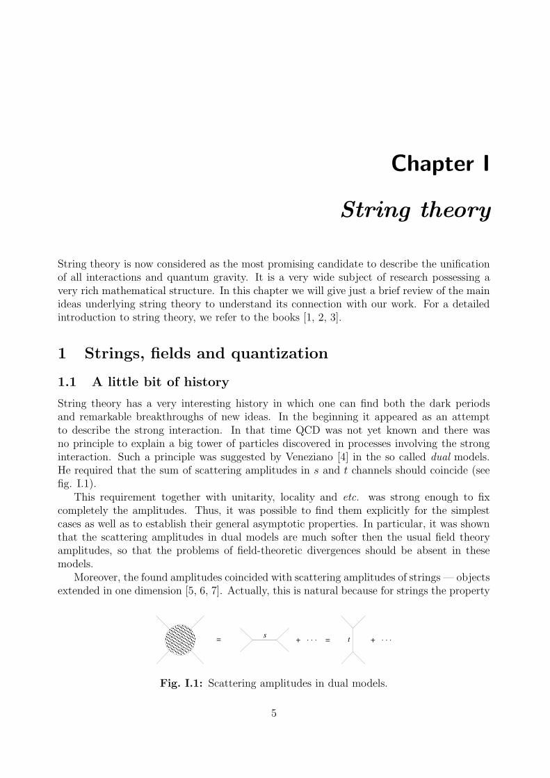
String theory has a very interesting history in which one can find both the dark periodsand remarkable breakthroughs of new ideas. In the beginning it appeared as an attemptto describe the strong interaction. In that time QCD was not yet known and there wasno principle to explain a big tower of particles discovered in processes involving the stronginteraction. Such a principle was suggested by Veneziano [4] in the so called dual models.He required that the sum of scattering amplitudes in s and t channels should coincide (seefig. I.1).
This requirement together with unitarity, locality and etc. was strong enough to fixcompletely the amplitudes. Thus, it was possible to find them explicitly for the simplestcases as well as to establish their general asymptotic properties. In particular, it was shownthat the scattering amplitudes in dual models are much softer then the usual field theoryamplitudes, so that the problems of field-theoretic divergences should be absent in thesemodels.
Moreover, the found amplitudes coincided with scattering amplitudes of strings — objectsextended in one dimension [5, 6, 7]. Actually, this is natural because for strings the property
t. . .+ . . .+
= s =
Fig. I.1: Scattering amplitudes in dual models.
5

Chapter I: String theory
s t
Fig. I.2: Scattering string amplitude can be seen in two ways.
of duality is evident: two channels can be seen as two degenerate limits of the same stringconfiguration (fig. I.2). Also the absence of ultraviolet divergences got a natural explanationin this picture. In field theory the divergences appear due to a local nature of interactionsrelated to the fact that the interacting objects are thought to be pointlike. When particles(pointlike objects) are replaced by strings the singularity is smoothed out over the stringworld sheet.
However, this nice idea was rejected by the discovery of QCD and description of allstrongly interacting particles as composite states of fundamental quarks. Moreover, theexponential fall-off of string amplitudes turned out to be inconsistent with the observedpower-like asymptotics. Thus, strings lost the initial reason to be related to fundamentalphysics.
But suddenly another reason was found. Each string possesses a spectrum of excitations.All of them can be interpreted as particles with different spins and masses. For a closedstring, which can be thought just as a circle, the spectrum contains a massless mode of spin2. But the graviton, quantum of gravitational interaction, has the same quantum numbers.Therefore, strings might be used to describe quantum gravity! If this is so, a theory basedon strings should describe the world at the very microscopic level, such as the Planck scale,and should reproduce the standard model only in some low-energy limit.
This idea gave a completely new status to string theory. It became a candidate for theunified theory of all interactions including gravity. Since that time string theory has beendeveloped into a rich theory and gave rise to a great number of new physical concepts. Letus have a look how it works.
1.2 String action
As is well known, the action for the relativistic particle is given by the length of its worldline. Similarly, the string action is given by the area of its world sheet so that classicaltrajectories correspond to world sheets of minimal area. The standard expression for thearea of a two-dimensional surface leads to the action [8, 9]
SNG = − 1
2πα′
∫
Σdτdσ
√−h, h = det hab, (I.1)
which is called the Nambu–Goto action. Here α′ is a constant of dimension of squared length.The matrix hab is the metric induced on the world sheet and can be represented as
hab = Gµν∂aXµ∂bX
ν, (I.2)
6

§1 Strings, fields and quantization
a) b)
Fig. I.3: Open and closed strings.
where Xµ(τ, σ) are coordinates of a point (τ, σ) on the world sheet in the spacetime wherethe string moves. Such a spacetime is called target space and Gµν(X) is the metric there.
Due to the square root even in the flat target space the action (I.1) is highly non-linear.Fortunately, there is a much more simple formulation which is classically equivalent to theNambu–Goto action. This is the Polyakov action [10]:
SP = − 1
4πα′
∫
Σdτdσ
√−hGµνh
ab∂aXµ∂bX
ν. (I.3)
Here the world sheet metric is considered as a dynamical variable and the relation (I.2)appears only as a classical equation of motion. (More exactly, it is valid only up to someconstant multiplier.) This means that we deal with a gravitational theory on the world sheet.We can even add the usual Einstein term
χ =1
4π
∫
Σdτdσ
√−hR. (I.4)
In two dimensions√−hR is a total derivative. Therefore, χ depends only on the topology of
the surface Σ, which one integrates over, and produces its Euler characteristic. In fact, anycompact connected oriented two-dimensional surface can be represented as a sphere with ghandles and b boundaries. In this case the Euler characteristic is
χ = 2 − 2g − b. (I.5)
Thus, the full string action reads
SP = − 1
4πα′
∫
Σdτdσ
√−h
(
Gµνhab∂aX
µ∂bXν + α′νR
)
, (I.6)
where we introduced the coupling constant ν. In principle, one could add also a two-dimensional cosmological constant. However, in this case the action would not be equivalentto the Nambu–Goto action. Therefore, we leave this possibility aside.
To completely define the theory, one should also impose some boundary conditions on thefields Xµ(τ, σ). There are two possible choices corresponding to two types of strings whichone can consider. The first choice is to take Neumann boundary conditions na∂aX
µ = 0on ∂Σ, where na is the normal to the boundary. The presence of the boundary meansthat one considers an open string with two ends (fig. I.3a). Another possibility is given byperiodic boundary conditions. The corresponding string is called closed and it is topologicallyequivalent to a circle (fig. I.3b).
7

Chapter I: String theory
1.3 String theory as two-dimensional gravity
The starting point to write the Polyakov action was to describe the movement of a stringin a target space. However, it possesses also an additional interpretation. As we alreadymentioned, the two-dimensional metric hab in the Polyakov formulation is a dynamical vari-able. Besides, the action (I.6) is invariant under general coordinate transformations on theworld sheet. Therefore, the Polyakov action can be equally considered as describing two-dimensional gravity coupled with matter fields Xµ. The matter fields in this case are usualscalars. The number of these scalars coincides with the dimension of the target space.
Thus, there are two dual points of view: target space and world sheet pictures. In thesecond one we can actually completely forget about strings and consider it as the problemof quantization of two-dimensional gravity in the presence of matter fields.
It is convenient to make the analytical continuation to the Euclidean signature on theworld sheet τ → −iτ . Then the path integral over two-dimensional metrics can be betterdefined, because the topologically non-trivial surfaces can have non-singular Euclidean met-rics, whereas in the Minkowskian signature their metrics are always singular. In this waywe arrive at a statistical problem for which the partition function is given by a sum overfluctuating two-dimensional surfaces and quantum fields on them1
Z =∑
surfaces Σ
∫
DXµ e−S(E)
P [X,Σ]. (I.7)
The sum over surfaces should be understood as a sum over all possible topologies plus afunctional integral over metrics. In two dimensions all topologies are classified. For example,for closed oriented surfaces the sum over topologies corresponds to the sum over genera gwhich is the number of handles attached to a sphere. In this case one gets
∑
surfaces Σ
=∑
g
∫
D%(hab). (I.8)
On the contrary, the integral over metrics is yet to be defined. One way to do this is todiscretize surfaces and to change the integral by the sum over discretizations. This way leadsto matrix models discussed in the following chapters.
In string theory one usually follows another approach. It treats the two-dimensionaldiffeomorphism invariance as ordinary gauge symmetry. Then the standard Faddeev–Popovgauge fixing procedure is applied to make the path integral to be well defined. However, thePolyakov action possesses an additional feature which makes its quantization non-trivial.
1.4 Weyl invariance
The Polyakov action (I.6) is invariant under the local Weyl transformations
hab −→ eφhab, (I.9)
where φ(τ, σ) is any function on the world sheet. This symmetry is very crucial because itallows to exclude one more degree of freedom. Together with the diffeomorphism symmetry,
1Note, that the Euclidean action S(E)P differs by sign from the Minkowskian one.
8
§1 Strings, fields and quantization
it leads to the possibility to express at the classical level the world sheet metric in terms ofderivatives of the spacetime coordinates as in (I.2). Thus, it is responsible for the equivalenceof the Polyakov and Nambu–Goto actions.
However, the classical Weyl symmetry can be broken at the quantum level. The reasoncan be found in the non-invariance of the measure of integration over world sheet metrics.Due to the appearance of divergences the measure should be regularized. But there is noregularization preserving all symmetries including the conformal one.
The anomaly can be most easily seen analyzing the energy-momentum tensor Tab. In anyclassical theory invariant under the Weyl transformations the trace of Tab should be zero.Indeed, the energy-momentum tensor is defined by
Tab = − 2π√−h
δS
δhab. (I.10)
If the metric is varied along eq. (I.9) (φ should be taken infinitesimal), one gets
T aa =
2π√−h
δS
δφ= 0. (I.11)
However, in quantum theory Tab should be replaced by a renormalized average of the quantumoperator of the energy-momentum tensor. Since the renormalization in general breaks theWeyl invariance, the trace will not vanish anymore.
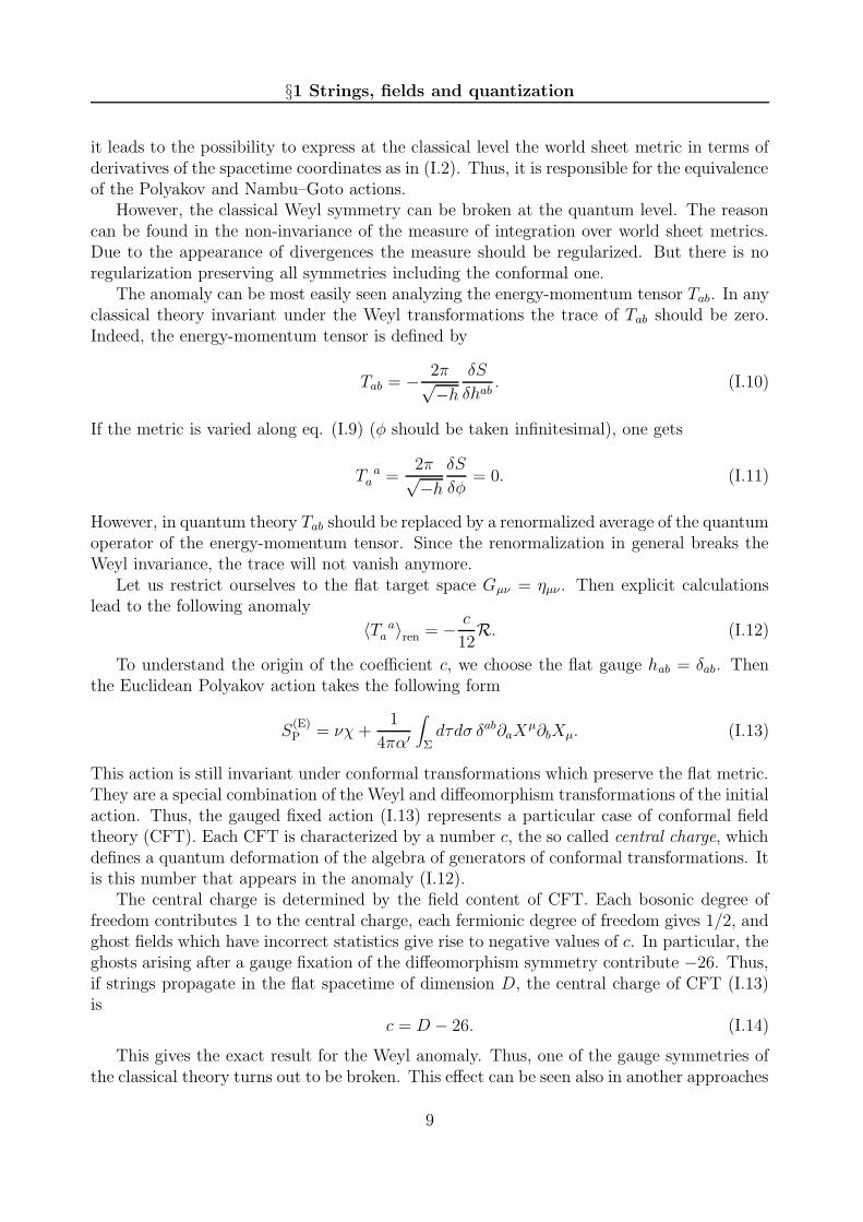
Let us restrict ourselves to the flat target space Gµν = ηµν . Then explicit calculationslead to the following anomaly
〈T aa 〉ren = − c
12R. (I.12)
To understand the origin of the coefficient c, we choose the flat gauge hab = δab. Thenthe Euclidean Polyakov action takes the following form
S(E)P = νχ +
1
4πα′
∫
Σdτdσ δab∂aX
µ∂bXµ. (I.13)
This action is still invariant under conformal transformations which preserve the flat metric.They are a special combination of the Weyl and diffeomorphism transformations of the initialaction. Thus, the gauged fixed action (I.13) represents a particular case of conformal fieldtheory (CFT). Each CFT is characterized by a number c, the so called central charge, whichdefines a quantum deformation of the algebra of generators of conformal transformations. Itis this number that appears in the anomaly (I.12).
The central charge is determined by the field content of CFT. Each bosonic degree offreedom contributes 1 to the central charge, each fermionic degree of freedom gives 1/2, andghost fields which have incorrect statistics give rise to negative values of c. In particular, theghosts arising after a gauge fixation of the diffeomorphism symmetry contribute −26. Thus,if strings propagate in the flat spacetime of dimension D, the central charge of CFT (I.13)is
c = D − 26. (I.14)
This gives the exact result for the Weyl anomaly. Thus, one of the gauge symmetries ofthe classical theory turns out to be broken. This effect can be seen also in another approaches
9

Chapter I: String theory
to string quantization. For example, in the framework of canonical quantization in the flatgauge one finds the breakdown of unitarity. Similarly, in the light-cone quantization oneencounters the breakdown of global Lorentz symmetry in the target space. All this indicatesthat the Weyl symmetry is extremely important for the existence of a viable theory of strings.
10

§2 Critical string theory
2 Critical string theory
2.1 Critical bosonic strings
We concluded the previous section with the statement that to consistently quantize stringtheory we need to preserve the Weyl symmetry. How can this be done? The expression forthe central charge (I.14) shows that it is sufficient to place strings into spacetime of dimensionDcr = 26 which is called critical dimension. Then there is no anomaly and quantum theoryis well defined.
Of course, our real world is four-dimensional. But now the idea of Kaluza [11] andKlein [12] comes to save us. Namely, one supposes that extra 22 dimensions are compactand small enough to be invisible at the usual scales. One says that the initial spacetimeis compactified. However, now one has to choose some compact space to be used in thiscompactification. It is clear that the effective four-dimensional physics crucially depends onthis choice. But a priori there is no any preference and it seems to be impossible to find theright compactification.
Actually, the situation is worse. Among modes of the bosonic string, which are interpretedas fields in the target space, there is a mode with a negative squared mass that is a tachyon.Such modes lead to instabilities of the vacuum and can break the unitarity. Thus, the bosonicstring theory in 26 dimensions is still a ”bad” theory.
2.2 Superstrings
An attempt to cure the problem of the tachyon of bosonic strings has led to a new theorywhere the role of fundamental objects is played by superstrings. A superstring is a gen-eralization of the ordinary bosonic string including also fermionic degrees of freedom. Itsimportant feature is a supersymmetry. In fact, there are two formulations of superstringtheory with the supersymmetry either in the target space or on the world sheet.
Green–Schwarz formulation
In the first formulation, developed by Green and Schwarz [13], to the fields Xµ one adds oneor two sets of world sheet scalars θA. They transform as Maiorana–Weyl spinors with respectto the global Lorentz symmetry in the target space. The number of spinors determines thenumber of supersymmetric charges so that there are two possibilities to have N = 1 orN = 2 supersymmetry. It is interesting that already at the classical level one gets somerestrictions on possible dimensions D. It can be 3, 4, 6 or 10. However, the quantizationselects only the last possibility which is the critical dimension for superstring theory.
In this formulation one has the explicit supersymmetry in the target space.2 Due to this,the tachyon mode cannot be present in the spectrum of superstring and the spectrum startswith massless modes.
2Superstring can be interpreted as a string moving in a superspace.
11

Chapter I: String theory
RNS formulation
Unfortunately, the Green–Schwarz formalism is too complicated for real calculations. Itis much more convenient to use another formulation with a supersymmetry on the worldsheet [14, 15]. It represents a natural extension of CFT (I.13) being a two-dimensionalsuper-conformal field theory (SCFT).3 In this case the additional degrees of freedom areworld sheet fermions ψµ which form a vector under the global Lorentz transformations inthe target space.
Since this theory is a particular case of conformal theories, the formula (I.12) for theconformal anomaly remains valid. Therefore, to find the critical dimension in this formalism,it is sufficient to calculate the central charge. Besides the fields discussed in the bosonic case,there are contributions to the central charge from the world sheet fermions and ghosts whicharise after a gauge fixing of the local fermionic symmetry. This symmetry is a superpartnerof the usual diffeomorphism symmetry and is a necessary part of supergravity. As wasmentioned, each fermion gives the contribution 1/2, whereas for the new superconformalghosts it is 11. As a result, one obtains
c = D − 26 +1
2D + 11 =
3
2(D − 10). (I.15)
This confirms that the critical dimension for superstring theory is Dcr = 10.To analyze the spectrum of this formulation, one should impose boundary conditions on
ψµ. But now the number of possibilities is doubled with respect to the bosonic case. Forexample, since ψµ are fermions, for the closed string not only periodic, but also antiperiodicconditions can be chosen. This leads to the existence of two independent sectors calledRamond (R) and Neveu–Schwarz (NS) sectors. In each sector superstrings have differentspectra of modes. In particular, from the target space point of view, R-sector describesfermions and NS-sector contains bosonic fields. But the latter suffers from the same problemas bosonic string theory — its lowest mode is a tachyon.
Is the fate of RNS formulation the same as that of the bosonic string theory in 26 di-mensions? The answer is not. In fact, when one calculates string amplitudes of perturbationtheory, one should sum over all possible spinor structures on the world sheet. This leads toa special projection of the spectrum, which is called Gliozzi–Scherk–Olive (GSO) projection[16]. It projects out the tachyon and several other modes. As a result, one ends up with awell defined theory.
Moreover, it can be checked that after the projection the theory possesses the globalsupersymmetry in the target space. This indicates that actually GS and RNS formulationsare equivalent. This can be proven indeed and is related to some intriguing symmetries ofsuperstring theory in 10 dimensions.
Consistent superstring theories
Once we have constructed general formalism, one can ask how many consistent theories ofsuperstrings do exist? Is it unique or not?
3In fact, it is two-dimensional supergravity coupled with superconformal matter. Thus, in this formulationone has a supersymmetric generalization of the interpretation discussed in section 1.3.
12

§2 Critical string theory
b)a)
Fig. I.4: Interactions of open and closed strings.
At the classical level it is certainly not unique. One has open and closed, oriented andnon-oriented, N = 1 and N = 2 supersymmetric string theories. Besides, in the openstring case one can also introduce Yang–Mills gauge symmetry adding charges to the endsof strings. It is clear that the gauge group is not fixed anyhow. Finally, considering closedstrings with N = 1 supersymmetry, one can construct the so called heterotic strings whereit is also possible to introduce a gauge group.
However, quantum theory in general suffers from anomalies arising at one and higherloops in string perturbation theory. The requirement of anomaly cancellation forces torestrict ourselves only to the gauge group SO(32) in the open string case and SO(32) orE8×E8 in the heterotic case [17]. Taking into account also restrictions on possible boundaryconditions for fermionic degrees of freedom, one ends up with five consistent superstringtheories. We give their list below:
• type IIA: N = 2 oriented non-chiral closed strings;
• type IIB: N = 2 oriented chiral closed strings;
• type I: N = 1 non-oriented open strings with the gauge group SO(32) + non-orientedclosed strings;
• heterotic SO(32): heterotic strings with the gauge group SO(32);
• heterotic E8 × E8: heterotic strings with the gauge group E8 × E8.
2.3 Branes, dualities and M-theory
Since there are five consistent superstring theories, the resulting picture is not completelysatisfactory. One should either choose a correct one among them or find a further unifica-tion. Besides, there is another problem. All string theories are defined only as asymptoticexpansions in string coupling constant. This expansion is nothing else but the sum overgenera of string world sheet in the closed case (see (I.8)) and over the number of boundariesin the open case. It is associated with string loop expansion since adding a handle (strip)can be interpreted as two subsequent interactions: a closed (open) string is emitted and thenreabsorbed (fig. I.4).
Note, that from the action (I.13) it follows that each term in the partition function (I.7)is weighted by the factor e−νχ which depends only on the topology of the world sheet. Due
13
Chapter I: String theory
S1 S1
IIB IIA
D=11
SO(32)
SO(32)I
het
het
E8 E8TT
/ Z 2
S
Fig. I.5: Chain of dualities relating all superstring theories.
to this one can associate e2ν with each handle and eν with each strip. On the other hand,each interaction process should involve a coupling constant. Therefore, ν determines theclosed and open string coupling constants
gcl ∼ eν , gop ∼ eν/2. (I.16)
Since string theories are defined as asymptotic expansions, any finite value of ν leads totroubles. Besides, it looks like a free parameter and there is no way to fix its value.
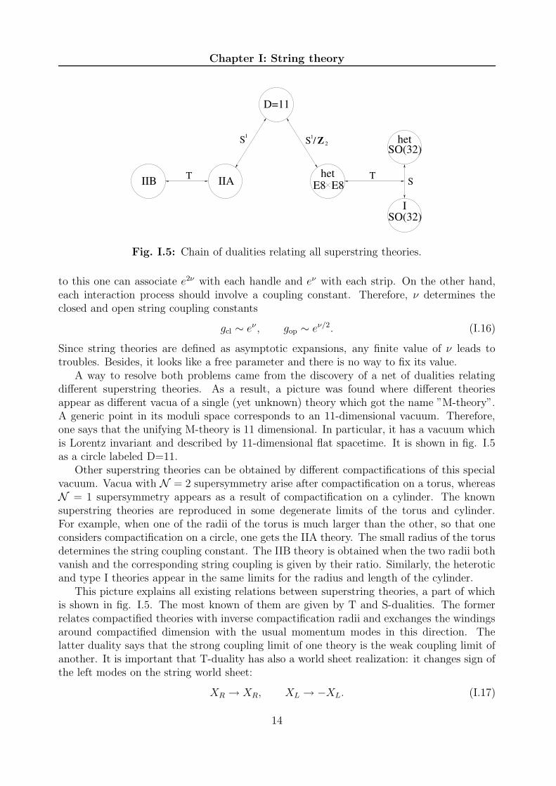
A way to resolve both problems came from the discovery of a net of dualities relatingdifferent superstring theories. As a result, a picture was found where different theoriesappear as different vacua of a single (yet unknown) theory which got the name ”M-theory”.A generic point in its moduli space corresponds to an 11-dimensional vacuum. Therefore,one says that the unifying M-theory is 11 dimensional. In particular, it has a vacuum whichis Lorentz invariant and described by 11-dimensional flat spacetime. It is shown in fig. I.5as a circle labeled D=11.
Other superstring theories can be obtained by different compactifications of this specialvacuum. Vacua with N = 2 supersymmetry arise after compactification on a torus, whereasN = 1 supersymmetry appears as a result of compactification on a cylinder. The knownsuperstring theories are reproduced in some degenerate limits of the torus and cylinder.For example, when one of the radii of the torus is much larger than the other, so that oneconsiders compactification on a circle, one gets the IIA theory. The small radius of the torusdetermines the string coupling constant. The IIB theory is obtained when the two radii bothvanish and the corresponding string coupling is given by their ratio. Similarly, the heteroticand type I theories appear in the same limits for the radius and length of the cylinder.
This picture explains all existing relations between superstring theories, a part of whichis shown in fig. I.5. The most known of them are given by T and S-dualities. The formerrelates compactified theories with inverse compactification radii and exchanges the windingsaround compactified dimension with the usual momentum modes in this direction. Thelatter duality says that the strong coupling limit of one theory is the weak coupling limit ofanother. It is important that T-duality has also a world sheet realization: it changes sign ofthe left modes on the string world sheet:
XR → XR, XL → −XL. (I.17)
14

§2 Critical string theory
The above picture indicates that the string coupling constant is always determined bythe background on which string theory is considered. Thus, it is not a free parameter butone of the moduli of the underlying M-theory.
It is worth to note that the realization of the dualities was possible only due to thediscovery of new dynamical objects in string theory — D branes [18]. They appear in severalways. On the one hand, they are solitonic solutions of supergravity equations determiningpossible string backgrounds. On the other hand, they are objects where open strings canend. In this case Dirichlet boundary conditions are imposed on the fields propagating on theopen string world sheet. Already at this point it is clear that such objects must present in thetheory because the T-duality transformation (I.17) exchanges the Neumann and Dirichletboundary conditions.
We stop our discussion of critical superstring theories here. We see that they allow fora nice unified picture of all interactions. However, the final theory remains to be hiddenfrom us and we even do not know what principles should define it. Also a correct way tocompactify extra dimensions to get the 4-dimensional physics is not yet found.
15

Chapter I: String theory
3 Low-energy limit and string backgrounds
3.1 General σ-model
In the previous section we discussed string theory in the flat spacetime. What changes ifthe target space is curved? We will concentrate here only on the bosonic theory. Addingfermions does not change much in the conclusions of this section.
In fact, we already defined an action for the string moving in a general spacetime. It isgiven by the σ-model (I.6) with an arbitrary Gµν(X). On the other hand, one can thinkabout a non-trivial spacetime metric as a coherent state of gravitons which appear in theclosed string spectrum. Thus, the insertion of the metric Gµν into the world sheet action is,roughly speaking, equivalent to summing of excitations of this mode.
But the graviton is only one of the massless modes of the string spectrum. For theclosed string the spectrum contains also two other massless fields: the antisymmetric tensorBµν and the scalar dilaton Φ. There is no reason to turn on the first mode and to leaveother modes non-excited. Therefore, it is more natural to write a generalization of (I.6)which includes also Bµν and Φ. It is given by the most general world sheet action which isinvariant under general coordinate transformations and renormalizable [19]:4
Sσ =1
4πα′
∫
d2σ√h[(
habGµν(X) + iεabBµν(X))
∂aXµ∂bX
ν + α′RΦ(X)]
, (I.18)
In contrast to the Polyakov action in flat spacetime, the action (I.18) is non-linear andrepresents an interacting theory. The couplings of this theory are coefficients of Gµν , Bµν andΦ of their expansion in Xµ. These coefficients are dimensionfull and the actual dimensionlesscouplings are their combinations with the parameter α′. This parameter has dimension ofsquared length and determines the string scale. It is clear that the perturbation expansionof the world sheet quantum field theory is an expansion in α′ and, at the same time, itcorresponds to the long-range or low-energy expansion in the target space. At large distancescompared to the string scale, the internal structure of the string is not important and weshould obtain an effective theory. This theory is nothing else but an effective field theory ofmassless string modes.
3.2 Weyl invariance and effective action
The effective theory, which appears in the low-energy limit, should be a theory for fieldsin the target space. On the other hand, from the world sheet point of view, these fieldsrepresent an infinite set of couplings of a two-dimensional quantum field theory. Therefore,equations of the effective theory should be some constraints on the couplings.
What are these constraints? The only condition, which is not imposed by hand, is thatthe σ-model (I.18) should define a consistent string theory. In particular, this means thatthe resulting quantum theory preserves the Weyl invariance. It is this requirement that givesthe necessary equations on the target space fields.
With each field one can associate a β-function. The Weyl invariance requires the vanish-ing of all β-functions [20]. These are the conditions we were looking for. In the first order
4In the following, the world sheet metric is always implied to be Euclidean.
16

§3 Low-energy limit and string backgrounds
in α′ one can find the following equations
βGµν = Rµν + 2∇µ∇νΦ − 1
4HµλσHν
λσ +O(α′) = 0,
βBµν = −1
2∇λHµν
λ +Hµνλ∇λΦ +O(α′) = 0, (I.19)
βΦ =D − 26
6α′ − 1
4R−∇2Φ + (∇Φ)2 +
1
48HµνλH
µνλ +O(α′) = 0,
whereHµνλ = ∂µBνλ + ∂λBµν + ∂νBλµ (I.20)
is the field strength for the antisymmetric tensor Bµν.A very non-trivial fact which, on the other hand, can be considered as a sign of consistency
of the approach, is that the equations (I.19) can be derived from the spacetime action [19]
Seff =1
2
∫
dDX√−Ge−2Φ
[
−2(D − 26)
3α′ +R + 4(∇Φ)2 − 1
12HµνλH
µνλ
]
. (I.21)
All terms in this action are very natural representing the simplest Lagrangians for symmetricspin-2, scalar, and antisymmetric spin-2 fields. The first term plays the role of the cosmo-logical constant. It is huge in the used approximation since it is proportional to α′−1. Butjust in the critical dimension it vanishes identically.
The only non-standard thing is the presence of the factor e−2Φ in front of the action.However, it can be removed by rescaling the metric. As a result, one gets the usual Ein-stein term what means that string theory reproduces Einstein gravity in the low-energyapproximation.
3.3 Linear dilaton background
Any solution of the equations (I.19) defines a consistent string theory. In particular, amongthem one finds the simplest flat, constant dilaton background
Gµν = ηµν , Bµν = 0, Φ = ν, (I.22)
which is a solution of the equations of motion only in Dcr = 26 dimensions reproducing thecondition we saw above.
There are also solutions which do not require any restriction on the dimension of space-time. To find them it is enough to choose a non-constant dilaton to cancel the first term inβΦ. Strictly speaking, it is not completely satisfactory because the first term has anotherorder in α′ and, if we want to cancel it, one has to take into account contributions from thenext orders. Nevertheless, there exist exact solutions which do not involve the higher orders.The most important solution is the so called linear dilaton background
Gµν = ηµν , Bµν = 0, Φ = lµXµ, (I.23)
where
lµlµ =
26 −D
6α′ . (I.24)
17

Chapter I: String theory
X D
couplingweak
couplingstrong
wall
~ log 1/µ
Fig. I.6: String propagation in the linear dilaton background in the presence of the tachyonmode. The non-vanishing tachyon produces a wall prohibiting the penetration into the regionof a large coupling constant.
Note that the dilaton is a generalization of the coupling constant ν in (I.6). Therefore,from (I.16) it is clear that this is the dilaton that defines the string coupling constant whichcan now vary in spacetime
gcl ∼ eΦ. (I.25)
But then for the solution (I.23) there is a region where the coupling diverges and the stringperturbation theory fails. This means that such background does not define a satisfactorystring theory. However, there is a way to cure this problem.
3.4 Inclusion of tachyon
When we wrote the renormalizable σ-model (I.18), we actually missed one possible termwhich is a generalization of the two-dimensional cosmological constant
STσ =1
4πα′
∫
d2σ√h T (X). (I.26)
From the target space point of view, it introduces a tachyon field which is the lowest modeof bosonic strings. One can repeat the analysis of section 3.2 and calculate the contributionsof this term to the β-functions. Similarly to the massless modes, all of them can be deducedfrom the spacetime action which should be added to (I.21)
Stach = −1
2
∫
dDX√−Ge−2Φ
[
(∇T )2 − 4
α′T2]
. (I.27)
Let us consider the tachyon as a field moving in the fixed linear dilaton background.Substituting (I.23) into the action (I.27), one obtains the following equation of motion
∂2T − 2lµ∂µT +4
α′T = 0. (I.28)
18
§3 Low-energy limit and string backgrounds
It is easy to find its general solution
T = µ exp(pµXµ), (p− l)2 =
2 −D
6α′ . (I.29)
Together with (I.23), (I.29) defines a generalization of the linear dilaton background. Strictlyspeaking, it is not a solution of the equations of motion derived from the common actionSeff + Stach. However, this action includes only the first order in α′, whereas, in general, aswe discussed above, one should take into account higher order contributions. The necessityto do this is seen from the fact that the background fields (I.23) and (I.29) involve α′ ina non-trivial way. The claim is that they give an exact string background. Indeed, in thisbackground the complete σ-model action takes the form
S l.d.σ =
1
4πα′
∫
d2σ√h[
hab∂aXµ∂bXµ + α′RlµXµ + µepµXµ
]
. (I.30)
It can be checked that it represents an exact CFT and, consequently, defines a consistentstring theory.
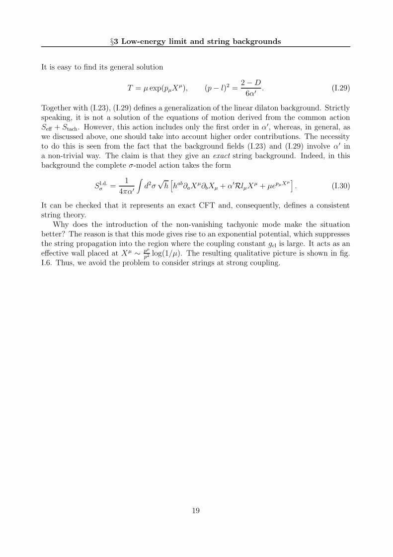
Why does the introduction of the non-vanishing tachyonic mode make the situationbetter? The reason is that this mode gives rise to an exponential potential, which suppressesthe string propagation into the region where the coupling constant gcl is large. It acts as aneffective wall placed at Xµ ∼ pµ
p2log(1/µ). The resulting qualitative picture is shown in fig.
I.6. Thus, we avoid the problem to consider strings at strong coupling.
19
Chapter I: String theory
4 Non-critical string theory
In the previous section we saw that, if to introduce non-vanishing expectation values forthe dilaton and tachyon, it is possible to define consistent string theory not only in thespacetime of critical dimension Dcr = 26. Still one can ask the question: is there any sensefor a theory where the conformal anomaly is not canceled? For example, if we look at the σ-model just as a statistical system of two-dimensional surfaces embedded into d-dimensionalspace and having some internal degrees of freedom, there is no reason for the system to beWeyl-invariant. Therefore, even in the presence of the Weyl anomaly, the system shouldpossess some interpretation. It is called non-critical string theory.
When one uses the interpretation we just described, even at the classical level one canintroduce terms breaking the Weyl invariance such as the world sheet cosmological constant.Then the conformal mode of the metric becomes a dynamical field and one should gaugefix only the world sheet diffeomorphisms. It can be done, for example, using the conformalgauge
hab = eφ(σ)hab. (I.31)
As a result, one obtains an effective action where, besides the matter fields, there is acontribution depending on φ [10]. Let us work in the flat target space. Then, after a suitablerescaling of φ to get the right kinetic term, the action is written as
SCFT =1
4πα′
∫
d2σ
√
h[
hab∂aXµ∂bXµ + hab∂aφ∂bφ− α′QRφ+ µeγφ + ghosts
]
. (I.32)
The second and third terms, which give dynamics to the conformal mode, come from themeasure of integration over all fields due to its non-invariance under the Weyl transforma-tions. The coefficient Q can be calculated from the conformal anomaly and is given by
Q =
√
25 − d
6α′ . (I.33)
The coefficient γ is fixed by the condition that the theory should depend only on the fullmetric hab. This means that the effective action (I.32) should be invariant under the followingWeyl transformations
hab(σ) −→ eρ(σ)hab(σ), φ(σ) −→ φ(σ) − ρ(σ). (I.34)
This implies that the action (I.32) defines CFT. This is indeed the case only if
γ = − 1√6α′
(√25 − d−
√1 − d
)
. (I.35)
The CFT (I.32) is called Liouville theory coupled with c = d matter. The conformal modeφ is the Liouville field.
The comparison of the two CFT actions (I.32) and (I.30) shows that they are equivalentif one takes D = d+ 1, pµ ∼ lµ and identifies XD = φ. Then all coefficients also coincide asfollows from (I.24), (I.29), (I.33) and (I.35). Thus, the conformal mode of the world sheetmetric can be interpreted as an additional spacetime coordinate. With this interpretationnon-critical string theory in the flat d-dimensional spacetime is seen as critical string theoryin the d + 1-dimensional linear dilaton background. The world sheet cosmological constantµ is identified with the amplitude of the tachyonic mode.
20

§5 Two-dimensional string theory
5 Two-dimensional string theory
In the following we will concentrate on the particular case of 2D bosonic string theory.It represents the main subject of this thesis. I hope to convince the reader that it has avery rich and interesting structure and, at the same time, it is integrable and allows formany detailed calculations.5 Thus, the two-dimensional case looks to be special and it is aparticular realization of a very universal structure. It appears in the description of differentphysical and mathematical problems. We will return to this question in the last chapter ofthe thesis. Here we just mention two interpretations which, as we have already seen, areequivalent to the critical string theory.
From the point of view of non-critical strings, 2D string theory is a model of fluctuatingtwo-dimensional surfaces embedded into 1-dimensional time. The second space coordinatearises from the metric on the surfaces.
Another possible interpretation of this system described in section 1.3 considers it astwo-dimensional gravity coupled with the c = 1 matter. The total central charge vanishessince the Liouville field φ, arising due to the conformal anomaly, contributes 1 + 6α′Q2,where Q is given in (I.33), and cancels the contribution of matter and ghosts.
5.1 Tachyon in two-dimensions
To see that the two-dimensional case is indeed very special, let us consider the effectiveaction (I.27) for the tachyon field in the linear dilaton background
Stach = −1
2
∫
dDX e2Qφ[
(∂T )2 − 4
α′T2]
, (I.36)
where φ is the target space coordinate coinciding with the gradient of the dilaton. Accordingto the previous section, it can be considered as the conformal mode of the world sheet metricof non-critical strings. After the redefinition T = e−Qφη, the tachyon action becomes anaction of a scalar field in the flat spacetime
Stach = −1
2
∫
dDX[
(∂η)2 +m2ηη
2]
, (I.37)
where
m2η = Q2 − 4
α′ =2 −D
6α′ (I.38)
is the mass of this field. For D > 2 the field η has an imaginary mass being a real tachyon.However, for D = 2 it becomes massless. Although we will still call this mode ”tachyon”,strictly speaking, it represents a good massless field describing the stable vacuum of thetwo-dimensional bosonic string theory. As always, the appearance in the spectrum of theadditional massless field indicates that the theory acquires some special properties.
In fact, the tachyon is the only field theoretic degree of freedom of strings in two dimen-sions. This is evident in the light cone gauge where there are physical excitations associated
5There is the so called c = 1 barrier which coincides with 2D string theory. Whereas string theories withc ≤ 1 are solvable, we cannot say much about c > 1 cases.
21

Chapter I: String theory
with D − 2 transverse oscillations and the motion of the string center of mass. The formerare absent in our case and the latter is identified with the tachyon field.
To find the full spectrum of states and the corresponding vertex operators, one shouldinvestigate the CFT (I.32) with one matter field X. The theory is well defined when thekinetic term for the X field enters with the + sign so that X plays the role of a spacecoordinate. Thus, we will consider the following CFT
SCFT =1
4π
∫
d2σ
√
h[
hab∂aX∂bX + hab∂aφ∂bφ− 2Rφ+ µe−2φ + ghosts]
, (I.39)
where we chose α′ = 1 and took into account that in two dimensions Q = 2, γ = −2.This CFT describes the Euclidean target space. The Minkowskian version is defined by theanalytical continuation X → it.
The CFT (I.39) is a difficult interacting theory due to the presence of the Liouville termµe−2φ. Nevertheless, one can note that in the region φ → ∞ this interaction is negligibleand the theory becomes free. Since the interaction is arbitrarily weak in the asymptotics,it cannot create or destroy states concentrated in this region. However, it removes from thespectrum all states concentrated at the opposite side of the Liouville direction. Therefore,it is sufficient to investigate the spectrum of the free theory with µ = 0 and impose the socalled Seiberg bound which truncates the spectrum by half [21].
The (asymptotic form of) vertex operators of the tachyon have already been found in(I.29). If lµ = (0,−Q) and pµ = (pX , pφ), one obtains the equation
p2X + (pφ +Q)2 = 0 (I.40)
with the general solution (Q = 2)
pX = ip, pφ = −2 ± |p|, p ∈ R. (I.41)
Imposing the Seiberg bound forbidding the operators growing at φ→ −∞, we have to choosethe + sign in (I.41). Thus, the tachyon vertex operators are
Vp =∫
d2σ eipXe(|p|−2)φ. (I.42)
Here p is the Euclidean momentum of the tachyon. When we go to the Minkowskian signa-ture, the momentum should also be continued as follows
X → it, p→ −ik. (I.43)
As a result, the vertex operators take the form
V −k =
∫
d2σ eik(t−φ)e−2φ,V +k =
∫
d2σ e−ik(t+φ)e−2φ,(I.44)
where k > 0. The two types of operators describe outgoing right movers and incoming leftmovers, respectively. They are used to calculate the scattering of tachyons off the Liouvillewall.
22
§5 Two-dimensional string theory
5.2 Discrete states
Although the tachyon is the only target space field in 2D string theory, there are also physicalstates which are remnants of the transverse excitations of the string in higher dimensions.They appear at special values of momenta and they are called discrete states [22, 23, 24, 25].
To define their vertex operators, we introduce the chiral fields
Wj,m = Pj,m(∂X, ∂2X, . . .)e2imXLe2(j−1)φL , (I.45)
Wj,m = Pj,m(∂X, ∂2X, . . .)e2imXRe2(j−1)φR , (I.46)
where j = 0, 12, 1, . . ., m = −j, . . . , j and we used the decomposition of the world sheet fields
into the chiral (left and right) components
X(τ, σ) = XR(τ − iσ) +XL(τ + iσ) (I.47)
and similarly for φ. Pj,m are polynomials in the chiral derivatives of X. Their dimension isj2 −m2. Due to this, Pj,±j = 1. For each fixed j, the set of operators Wj,m forms an SU(2)multiplet of spin j. Altogether, the operators (I.45) form W1+∞ algebra.
With the above definitions, the operators creating the discrete states are given by
Vj,m =∫
d2σWj,mWj,m, (I.48)
Thus, the discrete states appear at the following momenta
pX = 2im, pφ = 2(j − 1). (I.49)
It is clear that the lowest and highest components Vj,±j of each multiplet are just special casesof the vertex operators (I.42). The simplest non-trivial discrete state is the zero-momentumdilaton
V1,0 =∫
d2σ ∂X∂X. (I.50)
5.3 Compactification, winding modes and T-duality
So far we considered 2D string theory in the usual flat Euclidean or Minkowskian spacetime.The simplest thing which we can do with this spacetime is to compactify it. Since there isno translational invariance in the Liouville direction, it cannot be compactified. Therefore,we do compactification only for the Euclidean ”time” coordinate X. We require
X ∼ X + β, β = 2πR, (I.51)
where R is the radius of the compactification. Because it is the time direction that is com-pactified, we expect the resulting Minkowskian theory be equivalent to a thermodynamicalsystem at temperature T = 1/β.
The compactification restricts the allowed tachyon momenta to discrete values pn = n/Rso that we have only a discrete set of vertex operators. Besides, depending on the radius,the compactification can create or destroy the discrete states. Whereas for rational valuesof the radius some discrete states are present in the spectrum, for general irrational radiusthere are no discrete states.
23
Chapter I: String theory
But the compactification also leads to the existence of new physical string states. Theycorrespond to configurations where the string is wrapped around the compactified dimension.Such excitations are called winding modes. To describe these configurations in the CFTterms, one should use the decomposition (I.47) of the world sheet field X into the rightand left moving components. Then the operators creating the winding modes, the vortex
operators, are defined in terms of the dual field
X(τ, σ) = XR(τ − iσ) −XL(τ + iσ). (I.52)
They also have a discrete spectrum, but with the inverse frequency: qm = mR. In otherrespects they are similar to the vertex operators (I.42)
Vq =∫
d2σ eiqXe(|q|−2)φ. (I.53)
The vertex and vortex operators are related by T-duality, which exchanges the radiusof compactification R ↔ 1/R and the world sheet fields corresponding to the compactifieddirection X ↔ X (cf. (I.17)). Thus, from the CFT point of view it does not matter whethervertex or vortex operators are used to perturb the free theory. For example, the correlatorsof tachyons at the radius R should coincide with the correlators of windings at the radius1/R.6
Note that the self-dual radius R = 1 is distinguished by a higher symmetry of the systemin this case. As we will see, its mathematical description is especially simple.
6In fact, one should also change the cosmological constant µ → Rµ [26]. This change is equivalent to aconstant shift of the dilaton which is necessary to preserve the invariance to all orders in the genus expansion.
24

§6 2D string theory in non-trivial backgrounds
6 2D string theory in non-trivial backgrounds
6.1 Curved backgrounds: Black hole
In the previous section we described the basic properties of string theory in two-dimensionsin the linear dilaton background. In this thesis we will be interested in more general back-grounds. In the low-energy limit all of them can be described by an effective theory. Itsaction can be extracted from (I.21) and (I.27). Since there is no antisymmetric 3-tensor intwo dimensions, the B-field does not contribute and we remain with the following action
Seff =1
2
∫
d2X√−Ge−2Φ
[
16
α′ +R + 4(∇Φ)2 − (∇T )2 +4
α′T2]
. (I.54)
It is a model of dilaton gravity non-minimally coupled with a scalar field, the tachyon T .It is known to have solutions with non-vanishing curvature. Moreover, without the tachyonits general solution is well known and is written as [27] (Xµ = (t, r), Q = 2/
√α′)
ds2 = −(
1 − e−2Qr)
dt2 +1
1 − e−2Qrdr2, Φ = ϕ0 −Qr. (I.55)
In this form the solution resembles the radial part of the Schwarzschild metric for a sphericallysymmetric black hole. This is not a coincidence since the spacetime (I.55) does correspondto a two-dimensional black hole. At r = −∞ the curvature has a singularity and at r = 0the metric has a coordinate singularity corresponding to the black hole horizon. There isonly one integration constant ϕ0 which can be related to the mass of black hole
Mbh = 2Qe−2ϕ0 . (I.56)
As the usual Schwarzschild black hole, this black hole emits the Hawking radiation atthe temperature TH = Q
2π[28] and has a non-vanishing entropy [29, 30]. Thus, 2D string
theory incorporates all problems of the black hole thermodynamics and represents a model toapproach their solution. Compared to the quantum field theory analysis on curved spacetime,in string theory the situation is better since it is a well defined theory. Therefore, one canhope to solve the issues related to physics at Planck scale, such as microscopic descriptionof the black hole entropy, which are inaccessible by the usual methods.
To accomplish this task, one needs to know the background not only in the low-energylimit but also at all scales. Remarkably, an exact CFT, which reduces in the leading orderin α′ to the world sheet string action in the black hole background (I.55), was constructed[31]. It is given by the so called [SL(2,R)]k/U(1) coset σ-model where k is the level of therepresentation of the current algebra. Relying on this CFT, the exact form of the background(I.55), which ensures the Weyl invariance in all orders in α′, was found [32]. We write it inthe following form
ds2 = −l2(x)dt2 + dx2, l(x) = (1−p)1/2 tanhQx
(1−p tanh2 Qx)1/2 , (I.57)
Φ = ϕ0 − log coshQx− 14log(1 − p tanh2Qx), (I.58)
where p, Q and the level k are related by
p =2α′Q2
1 + 2α′Q2, k =
2
p= 2 +
1
α′Q2(I.59)
25
Chapter I: String theory
X
r=0
horizon
r
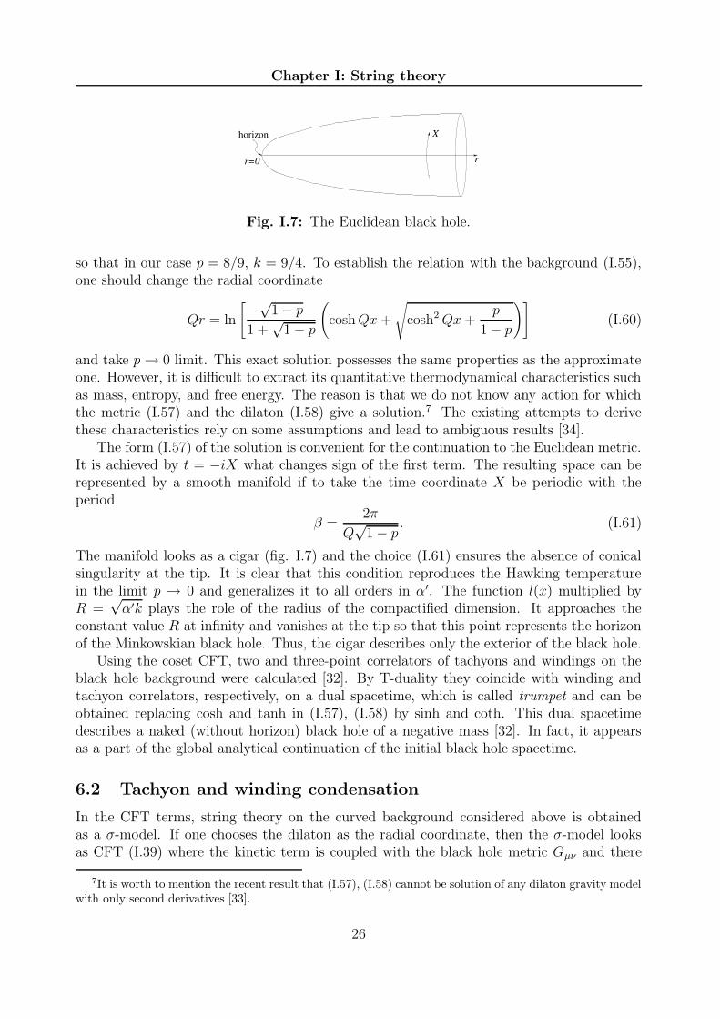
Fig. I.7: The Euclidean black hole.
so that in our case p = 8/9, k = 9/4. To establish the relation with the background (I.55),one should change the radial coordinate
Qr = ln
[ √1 − p
1 +√
1 − p
(
coshQx +
√
cosh2Qx +p
1 − p
)]
(I.60)
and take p→ 0 limit. This exact solution possesses the same properties as the approximateone. However, it is difficult to extract its quantitative thermodynamical characteristics suchas mass, entropy, and free energy. The reason is that we do not know any action for whichthe metric (I.57) and the dilaton (I.58) give a solution.7 The existing attempts to derivethese characteristics rely on some assumptions and lead to ambiguous results [34].
The form (I.57) of the solution is convenient for the continuation to the Euclidean metric.It is achieved by t = −iX what changes sign of the first term. The resulting space can berepresented by a smooth manifold if to take the time coordinate X be periodic with theperiod
β =2π
Q√
1 − p. (I.61)
The manifold looks as a cigar (fig. I.7) and the choice (I.61) ensures the absence of conicalsingularity at the tip. It is clear that this condition reproduces the Hawking temperaturein the limit p → 0 and generalizes it to all orders in α′. The function l(x) multiplied byR =
√α′k plays the role of the radius of the compactified dimension. It approaches the
constant value R at infinity and vanishes at the tip so that this point represents the horizonof the Minkowskian black hole. Thus, the cigar describes only the exterior of the black hole.
Using the coset CFT, two and three-point correlators of tachyons and windings on theblack hole background were calculated [32]. By T-duality they coincide with winding andtachyon correlators, respectively, on a dual spacetime, which is called trumpet and can beobtained replacing cosh and tanh in (I.57), (I.58) by sinh and coth. This dual spacetimedescribes a naked (without horizon) black hole of a negative mass [32]. In fact, it appearsas a part of the global analytical continuation of the initial black hole spacetime.
6.2 Tachyon and winding condensation
In the CFT terms, string theory on the curved background considered above is obtainedas a σ-model. If one chooses the dilaton as the radial coordinate, then the σ-model looksas CFT (I.39) where the kinetic term is coupled with the black hole metric Gµν and there
7It is worth to mention the recent result that (I.57), (I.58) cannot be solution of any dilaton gravity modelwith only second derivatives [33].
26
§6 2D string theory in non-trivial backgrounds
is no Liouville exponential interaction. The change of the metric can be represented as aperturbation of the linear dilaton background by the gravitational vertex operator. Notethat this operator creates one of the discrete states.
It is natural to consider also perturbations by another relevant operators existing in theinitial CFT (I.39) defined in the linear dilaton background. First of all, these are tachyonvertex operators Vp (I.42). Besides, if we consider the Euclidean theory compactified on acircle, there exist vortex operators Vq (I.53). Thus, the both types of operators can be usedto perturb the simplest CFT (I.39)
S = SCFT +∑
n6=0
(tnVn + tnVn), (I.62)
where we took into account that tachyons and windings have discrete spectra in the com-pactified theory.
What backgrounds of 2D string theory do these perturbations correspond to? The cou-plings tn introduce a non-vanishing vacuum expectation value of the tachyon. Thus, theysimply change the background value of T . Note that, in contrast to the cosmological con-stant term µe−2φ, these tachyon condensates are time-dependent. For the couplings tn wecannot give such a simple picture. The reason is that windings do not have a local targetspace interpretation. Therefore, it is not clear which local characteristics of the backgroundchange by the introduction of a condensate of winding modes.
A concrete proposal has been made for the simplest case t±1 6= 0, which is called Sine-
Liouville CFT. In [35] it was suggested that this CFT is equivalent to the SL(2,R)/U(1)σ-model describing string theory on the black hole background. This conjecture was justifiedby the coincidence of spectra of the two CFTs as well as of two and three-point correlators.Following this idea, it is natural to suppose that any general winding perturbation changesthe target space metric.
Note, that the world sheet T-duality relates the CFT (I.62) with one set of couplings(tn, tn) and radius of compactification R to the similar CFT, where the couplings are ex-changed (tn, tn) and the radius is inverse 1/R. However, these two theories should notdescribe the same background because the target space interpretations of tachyons andwindings are quite different. T-duality allows to relate their correlators, but it says nothinghow their condensation changes the target space.
27


Chapter II
Matrix models
In this chapter we introduce a powerful mathematical technique, which allows to solve manyphysical problems. Its main feature is the use of matrices of a large size. Therefore, themodels formulated using this technology are called matrix models. Sometimes a matrixformulation is not only a useful mathematical description of a physical system, but it alsosheds light on its fundamental degrees of freedom.
We will be interested mostly in application of matrix models to string theory. However,in the beginning we should explain their relation to physics, their general properties, andbasic methods to solve them (for an extensive review, see [36]). This is the goal of thischapter.
1 Matrix models in physics
Working with matrix models, one usually considers the situation when the size of matricesis very large. Moreover, these models imply integration over matrices or averaging overthem taking all matrix elements as independent variables. This means that one deals withsystems where some random processes are expected. Indeed, this is a typical behaviour forthe systems described by matrix models.
Statistical physics
Historically, for the first time matrix models appeared in nuclear physics. It was discoveredby Wigner [37] that the energy levels of large atomic nuclei are distributed according tothe same law, which describes the spectrum of eigenvalues of one Hermitian matrix in thelimit where the size of the matrix goes to infinity. Already this result showed the importantfeature of universality: it could be applied to any nucleus and did not depend on particularcharacteristics of this nucleus.
Following this idea, one can generalize the matrix description of statistics of energy levelsto any system, which either has many degrees of freedom and is too complicated for an exactdescription, or possesses a random behaviour. A typical example of systems of the firsttype is given by mesoscopic physics, where one is interested basically only in macroscopiccharacteristics. The second possibility is realized, in particular, in chaotic systems.
29

Chapter II: Matrix models
Quantum chromodynamics
Another subject, where matrix models gave a new method of calculation, is particle physics.The idea goes back to the work of ’t Hooft [38] where he suggested to use 1/N expansionfor calculations in gauge theory with the gauge group SU(N). Initially, he suggested thisexpansion for QCD as an alternative to the usual perturbative expansion, which is validonly in the weak coupling region and fails at low energies due to the confinement. However,in the case of QCD it is not well justified since the expansion parameter equals 1/32 and isnot very small.
Nevertheless, ’t Hooft realized several important facts about the 1/N expansion. First,SU(N) gauge theory can be considered as a model of N×N unitary matrices since the gaugefields are operators in the adjoint representation. Then the 1/N expansion corresponds tothe limit of large matrices. Second, it coincides with the topological expansion where allFeynman diagrams are classified according to their topology, which one can associate if alllines in Feynman diagrams are considered as double lines. This gives the so called fat graphs.In the limit N → ∞ only the planar diagrams survive. These are the diagrams which canbe drawn on the 2-sphere without intersections. Thus, with each matrix model one canassociate a diagrammatic expansion so that the size of matrices enters only as a prefactorfor each diagram.
Although this idea has not led to a large progress in QCD, it gave rise to new develop-ments, related with matrix models, in two-dimensional quantum gravity and string theory[39, 40, 41, 42, 43]. In turn, there is still a hope to find a connection between string theoryand QCD relying on matrix models [44]. Besides, recently they were applied to describesupersymmetric gauge theories [45].
Quantum gravity and string theory
The common feature of two-dimensional quantum gravity and string theory is a sum overtwo-dimensional surfaces. It turns out that it also has a profound connection with matrixmodels ensuring their relevance for these two theories. We describe this connection in detailin the next section because it deserves a special attention. Here we just mention that thereformulation of string theory in terms of matrix models has lead to significant results in thelow-dimensional cases such as 2D string theory. Unfortunately, this reformulation has nothelped much in higher dimensions.
It is worth to note that there are matrix models of M-theory [46, 47], which is thoughtto be a unification of all string theories (see section I.2.3). (See also [48, 49, 50] for earlierattempts to describe the quantum mechanics of the supermembranes.) They claim to befundamental non-perturbative and background independent formulations of Planck scalephysics. However, they are based on the ideas different from the ”old” matrix models oflow-dimensional string theories.
Also matrix models appear in the so called spin foam approach to 3 and 4-dimensionalquantum gravity [51, 52]. Similarly to models of M–theory, they give a non-perturbative andbackground independent formulation of quantum gravity but do not help with calculations.
30

§2 Matrix models and random surfaces
2 Matrix models and random surfaces
2.1 Definition of one-matrix model
Now it is time to define what a matrix model is. In the most simple case of one-matrix model
(1MM), one considers the following integral over N ×N matrices
Z =∫
dM exp [−N trV (M)] , (II.1)
where
V (M) =∑
k>0
gkkMk (II.2)
is a potential and the measure dM is understood as a product of the usual differentials ofall independent matrix elements
dM =∏
i,j
dMij. (II.3)
The integral (II.1) can be interpreted as the partition function in the canonical ensemble of astatistical model. Also it appears as a generating function for the correlators of the operatorstrMk, which are obtained differentiating Z with respect to the couplings gk. For generalcouplings, the integral (II.1) is divergent and should be defined by analytical continuation.
Actually, one can impose some restrictions on the matrix Mij which reflect the symmetryof the problem. Correspondingly, there exist 3 ensembles of random matrices:
• ensemble of hermitian matrices with the symmetry group U(N);
• ensemble of real symmetric matrices with the symmetry group O(N);
• ensemble of quaternionic matrices with the symmetry group Sp(N).
We will consider only the first ensemble. Therefore, our systems will always possess theglobal U(N) invariance under the transformations
M −→ Ω†MΩ (Ω†Ω = I). (II.4)
In general, the integral (II.1) cannot be evaluated exactly and one has to use its per-turbative expansion in coupling constants. Following the usual methodology of quantumfield theories, each term in this expansion can be represented as a Feynman diagram. Itsingredients, propagator and vertices, can be extracted from the potential (II.2). The maindifference with the case of a scalar field is that the propagator is represented by an orienteddouble line what reflects the index structure carried by matrices.
i
j k
l= 1
Ng2δilδjk
The expression which is associated with the propagator can be obtained as an average oftwo matrices 〈MijMkl〉0 with respect to the Gaussian part of the potential. The couplingof indices corresponds to the usual matrix multiplication law. The vertices come from the
31

Chapter II: Matrix models
terms of the potential of third and higher powers. They are also composed from the doublelines and are given by a product of Kronecker symbols.
ikjk
i1
j1
i2j2
i3j3
i4 j4
= N gk
kδj1i2δj2i3 · · · δjki1
Note that each loop in the diagrams gives the factor N coming from the sum over contractedindices. As a result, the partition function (II.1) is represented as
Z =∑
diagrams
1
s
(
1
Ng2
)E
NL∏
k
(−Ngk)nk , (II.5)
where the sum goes over all diagrams constructed from the drawn propagators and vertices(fat graphs) and we introduced the following notations:
• nk is the number of vertices with k legs in the diagram,
• V =∑
k nk is the total number of vertices,
• L is the number of loops,
• E = 12
∑
k knk is the number of propagators,
• s is the symmetry factor given by the order of the discrete group of symmetries of thediagram.
Thus, each diagram contributes to the partition function
1
sNV −E+Lg−E2
∏
k
(−gk)nk . (II.6)
2.2 Generalizations
Generalizations of the one-matrix model can be obtained by increasing the number of matri-ces. The simplest generalization is two-matrix model (2MM). In a general case it is definedby the following integral
Z =∫
dA dB exp [−NW (A,B)] , (II.7)
where W (A,B) is a potential invariant under the global unitary transformations
A −→ Ω†AΩ, B −→ Ω†BΩ. (II.8)
The structure of this model is already much richer than the structure of the one-matrixmodel. It will be important for us in the study of 2D string theory.
32
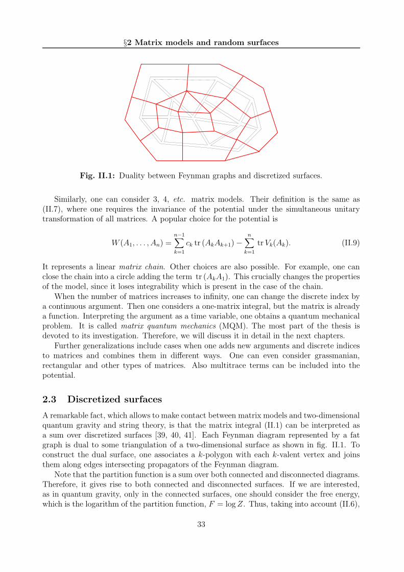
§2 Matrix models and random surfaces
Fig. II.1: Duality between Feynman graphs and discretized surfaces.
Similarly, one can consider 3, 4, etc. matrix models. Their definition is the same as(II.7), where one requires the invariance of the potential under the simultaneous unitarytransformation of all matrices. A popular choice for the potential is
W (A1, . . . , An) =n−1∑
k=1
ck tr (AkAk+1) −n∑
k=1
trVk(Ak). (II.9)
It represents a linear matrix chain. Other choices are also possible. For example, one canclose the chain into a circle adding the term tr (AkA1). This crucially changes the propertiesof the model, since it loses integrability which is present in the case of the chain.
When the number of matrices increases to infinity, one can change the discrete index bya continuous argument. Then one considers a one-matrix integral, but the matrix is alreadya function. Interpreting the argument as a time variable, one obtains a quantum mechanicalproblem. It is called matrix quantum mechanics (MQM). The most part of the thesis isdevoted to its investigation. Therefore, we will discuss it in detail in the next chapters.
Further generalizations include cases when one adds new arguments and discrete indicesto matrices and combines them in different ways. One can even consider grassmanian,rectangular and other types of matrices. Also multitrace terms can be included into thepotential.
2.3 Discretized surfaces
A remarkable fact, which allows to make contact between matrix models and two-dimensionalquantum gravity and string theory, is that the matrix integral (II.1) can be interpreted asa sum over discretized surfaces [39, 40, 41]. Each Feynman diagram represented by a fatgraph is dual to some triangulation of a two-dimensional surface as shown in fig. II.1. Toconstruct the dual surface, one associates a k-polygon with each k-valent vertex and joinsthem along edges intersecting propagators of the Feynman diagram.
Note that the partition function is a sum over both connected and disconnected diagrams.Therefore, it gives rise to both connected and disconnected surfaces. If we are interested,as in quantum gravity, only in the connected surfaces, one should consider the free energy,which is the logarithm of the partition function, F = logZ. Thus, taking into account (II.6),
33

Chapter II: Matrix models
the duality of matrix diagrams and discretized surfaces leads to the following representation
F =∑
surfaces
1
sNV−E+Lg−E2
∏
k
(−gk)nk . (II.10)
where we interpret:
• nk is the number of k-polygons used in the discretization,
• V =∑
k nk is the total number of polygons (faces),
• L is the number of vertices,
• E = 12
∑
k knk is the number of edges,
• s is the order of the group of automorphisms of the discretized surface.
It is clear that the relative numbers of k-polygons are controlled by the couplings gk. Forexample, if one wants to use only triangles, one should choose the cubic potential in thecorresponding matrix model.
The sum over discretizations (II.10) (more exactly, its continuum limit) can be consideredas a definition of the sum over surfaces appearing in (I.8). Each discretization induces acurvature on the surface, which is concentrated at vertices where several polygons are jointto each other. For example, if at ith vertex there are n
(i)k k-polygons, the discrete counterpart
of the curvature is
Ri = 2π
(
2 −∑
k
k−2kn
(i)k
)
∑
k
1kn
(i)k
. (II.11)
It counts the deficit angle at the given vertex. In the limit of large number of vertices,the discretization approximates some continuous geometry. Varying discretization, one canapproximate any continuous distribution of the curvature with any given accuracy.
Note, that the discretization encodes only the information about the curvature which isdiffeomorphism invariant. Therefore, the sum over discretizations realizes already a gaugefixed version of the path integral over geometries. Due to this, one does not need to dealwith ghosts and other problems related to gauge fixing.
If one considers generalizations of the one-matrix model, the dual surfaces will carryadditional structures. For example, the Feynman diagrams of two-matrix model are drawnusing two types of lines corresponding to two matrices. All vertices are constructed from thelines of a definite type since they come from the potential for either the first or the secondmatrix. Therefore, with each face of the dual discretization one can associate a discretevariable taking two values, say ±1. Summing over all structures, one obtains Ising modelon a random lattice [53, 54]. Similarly, it is possible to get various fields living on two-dimensional dynamical surfaces or, in other words, coupled with two-dimensional gravity.
34
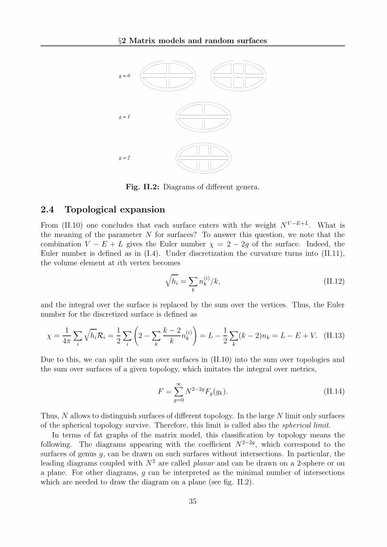
§2 Matrix models and random surfaces
g = 0
g = 1
g = 2
Fig. II.2: Diagrams of different genera.
2.4 Topological expansion
From (II.10) one concludes that each surface enters with the weight N V −E+L. What isthe meaning of the parameter N for surfaces? To answer this question, we note that thecombination V − E + L gives the Euler number χ = 2 − 2g of the surface. Indeed, theEuler number is defined as in (I.4). Under discretization the curvature turns into (II.11),the volume element at ith vertex becomes
√
hi =∑
k
n(i)k /k, (II.12)
and the integral over the surface is replaced by the sum over the vertices. Thus, the Eulernumber for the discretized surface is defined as
χ =1
4π
∑
i
√
hiRi =1
2
∑
i
(
2 −∑
k
k − 2
kn
(i)k
)
= L− 1
2
∑
k
(k − 2)nk = L− E + V. (II.13)
Due to this, we can split the sum over surfaces in (II.10) into the sum over topologies andthe sum over surfaces of a given topology, which imitates the integral over metrics,
F =∞∑
g=0
N2−2gFg(gk). (II.14)
Thus, N allows to distinguish surfaces of different topology. In the large N limit only surfacesof the spherical topology survive. Therefore, this limit is called also the spherical limit.
In terms of fat graphs of the matrix model, this classification by topology means thefollowing. The diagrams appearing with the coefficient N 2−2g, which correspond to thesurfaces of genus g, can be drawn on such surfaces without intersections. In particular, theleading diagrams coupled with N 2 are called planar and can be drawn on a 2-sphere or ona plane. For other diagrams, g can be interpreted as the minimal number of intersectionswhich are needed to draw the diagram on a plane (see fig. II.2).
35

Chapter II: Matrix models
2.5 Continuum and double scaling limits
Our goal is to relate the matrix integral to the sum over Riemann surfaces. We have alreadycompleted the first step reducing the matrix integral to the sum over discretized surfaces.And the sum over topologies was automatically included. It remains only to extract acontinuum limit.
To complete this second step, let us work for simplicity with the cubic potential
V (M) =1
2M2 − λ
3M3. (II.15)
Then (II.10) takes the form
F =∞∑
g=0
Nχ∑
genus gtriangulations
1
sλV . (II.16)
We compare this result with the partition function of two-dimensional quantum gravity
ZQG =∞∑
g=0
∫
D%(hab)e−νχ−µA, (II.17)
where g is the genus of the surface, A =∫
d2σ√h is its area, and ν and µ are coupling
constants. First of all, we see that one can identify N = e−ν. Then, if one assumes that alltriangles have unit area, the total area is given by the number of triangles V . Due to this,(II.16) implies λ = e−µ.
However, this was a formal identification because one needs the coincidence of the par-tition function ZQG and the free energy of the matrix model F . It is possible only in acontinuum limit where we sum over the same set of continuous surfaces. In this limit thearea of triangles used in the discretization should vanish. Since we fixed their area, in ourcase the continuum limit implies that the number of triangles should diverge V → ∞.
In quantum theory one can speak only about expectation values. Hence we are interestedin the behaviour of 〈V 〉. In fact, for the spherical topology this quantity is dominated by non-universal contributions. To see the universal behaviour related to the continuum limit, oneshould consider more general correlation functions 〈V n〉. From (II.16), for these quantitiesone obtains a simple expression
〈V n〉 =
(
λ∂
∂λ
)n
logF. (II.18)
The typical form of the contribution of genus g to the free energy is
Fg ∼ F (reg)g + (λc − λ)(2−γstr)χ/2, (II.19)
where γstr is the so called string susceptibility, which defines the critical behaviour, λc issome critical value of the coupling constant, and we took into account the non-universalcontribution F (reg)
g . The latter leads to the fact that the expectation value 〈V 〉 remainsfinite for χ > 0. But for all n > 1, one finds
〈V n〉〈V n−1〉 ∼ 1
λc − λ. (II.20)
36

§2 Matrix models and random surfaces
This shows that in the limit λ → λc, the sum (II.16) is dominated by triangulations withlarge number of triangles. Thus, the continuum limit is obtained taking λ → λc. One canrenormalize the area and the couplings so that they remain finite in this limit.
Now we encounter the following problem. According to (II.19), the (universal part ofthe) free energy in the continuum limit either diverges or vanishes depending on the genus.On the other hand, in the natural limit N → ∞ only the spherical contribution survives.How can one obtain contributions for all genera? It turns out that taking both limitsnot independently, but together in a correlated manner, one arrives at the desired result[55, 56, 57]. Indeed, we introduce the ”renormalized” string coupling
κ−1 = N(λc − λ)(2−γstr)/2, (II.21)
and consider the limit N → ∞, λ → λc, where κ is kept fixed. In this limit the free energyis written as an asymptotic expansion for κ→ 0
F =∞∑
g=0
κ−2+2gfg. (II.22)
Thus, the described limit allows to keep all genera in the expansion of the free energy. Itis called the double scaling limit. In this limit the free energy of the one-matrix modelreproduces the partition function of two-dimensional quantum gravity. This correspondenceholds also for various correlators and is extended to other models. In particular, the doublescaling limit of MQM, which we describe in the next chapter, gives 2D string theory.
The fact that nothing depends on the particular form of the potential, which is equivalentto the independence on the type of polygons used to discretize surfaces (triangles, quadran-gles, etc.), is known as universality of matrix models. All of them can be splitted into classesof universality. Each class is associated with some continuum theory and characterized bythe limiting behaviour of a matrix model near its critical point [58].
37

Chapter II: Matrix models
3 One-matrix model: saddle point approach
In the following two sections we review two basic methods to solve matrix models. This willbe done relying on explicit examples of the simplest matrix models, 1MM and 2MM. Thissection deals with the first model, which is defined by the integral over one hermitian matrix
Z =∫
dM exp [−N trV (M)] . (II.23)
The potential was given in (II.2). Since the matrix is hermitian, its independent matrixelements are Mij with i ≤ j and the diagonal elements are real. Therefore, the measure dMis given by
dM =∏
i
dMii
∏
i<j
dReMij d ImMij. (II.24)
3.1 Reduction to eigenvalues
Each hermitian matrix can be diagonalized by a unitary transformation
M = Ω†xΩ, x = diag(x1, . . . , xN), Ω†Ω = I. (II.25)
Therefore, one can change variables from the matrix elements Mij to the eigenvalues xkand elements of the unitary matrix Ω diagonalizing M . This change produces a Jacobian.To find it, one considers a hermitian matrix which is obtained by an infinitesimal unitarytransformation Ω = I + dω of the diagonal matrix x, where dω is antisymmetric. In the firstorder in ω, one obtains
dMij ≈ δijdxj + [x, dω]ij = δijdxj + (xi − xj)dωij. (II.26)
This leads to the following result
dM = [dΩ]SU(N)
N∏
k=1
dxk ∆2(x), (II.27)
where [dΩ]SU(N) is the Haar measure on SU(N) and
∆(x) =∏
i<j
(xi − xj) = deti,j
xj−1i (II.28)
is the Vandermonde determinant.Due to the U(N)-invariance of the potential, after the substitution (II.25) into the integral
(II.23) the unitary matrix Ω decouples and can be integrated out. As a result, one arrivesat the following representation
Z = Vol(SU(N))∫ N∏
k=1
dxk ∆2(x) exp
[
−NN∑
k=1
V (xk)
]
. (II.29)
The volume of the SU(N) group is a constant depending only on the matrix size N . It isnot relevant for the statistics of eigenvalues, although it is important for the dependence ofthe free energy on N .
The representation (II.29) is very important because it reduces the problem involvingN2 degrees of freedom to the problem of only N eigenvalues. This can be considered as a”generalized integrability”: models allowing such reduction are in a sense ”integrable”.
38
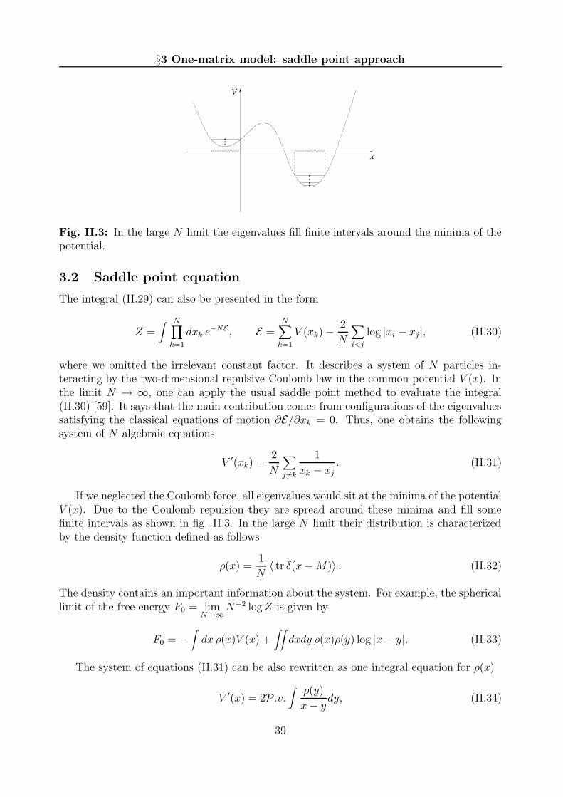
§3 One-matrix model: saddle point approach
V
x
Fig. II.3: In the large N limit the eigenvalues fill finite intervals around the minima of thepotential.
3.2 Saddle point equation
The integral (II.29) can also be presented in the form
Z =∫ N∏
k=1
dxk e−NE , E =
N∑
k=1
V (xk) −2
N
∑
i<j
log |xi − xj|, (II.30)
where we omitted the irrelevant constant factor. It describes a system of N particles in-teracting by the two-dimensional repulsive Coulomb law in the common potential V (x). Inthe limit N → ∞, one can apply the usual saddle point method to evaluate the integral(II.30) [59]. It says that the main contribution comes from configurations of the eigenvaluessatisfying the classical equations of motion ∂E/∂xk = 0. Thus, one obtains the followingsystem of N algebraic equations
V ′(xk) =2
N
∑
j 6=k
1
xk − xj. (II.31)
If we neglected the Coulomb force, all eigenvalues would sit at the minima of the potentialV (x). Due to the Coulomb repulsion they are spread around these minima and fill somefinite intervals as shown in fig. II.3. In the large N limit their distribution is characterizedby the density function defined as follows
ρ(x) =1
N〈 tr δ(x−M)〉 . (II.32)
The density contains an important information about the system. For example, the sphericallimit of the free energy F0 = lim
N→∞N−2 logZ is given by
F0 = −∫
dx ρ(x)V (x) +∫∫
dxdy ρ(x)ρ(y) log |x− y|. (II.33)
The system of equations (II.31) can be also rewritten as one integral equation for ρ(x)
V ′(x) = 2P.v.∫ ρ(y)
x− ydy, (II.34)
39
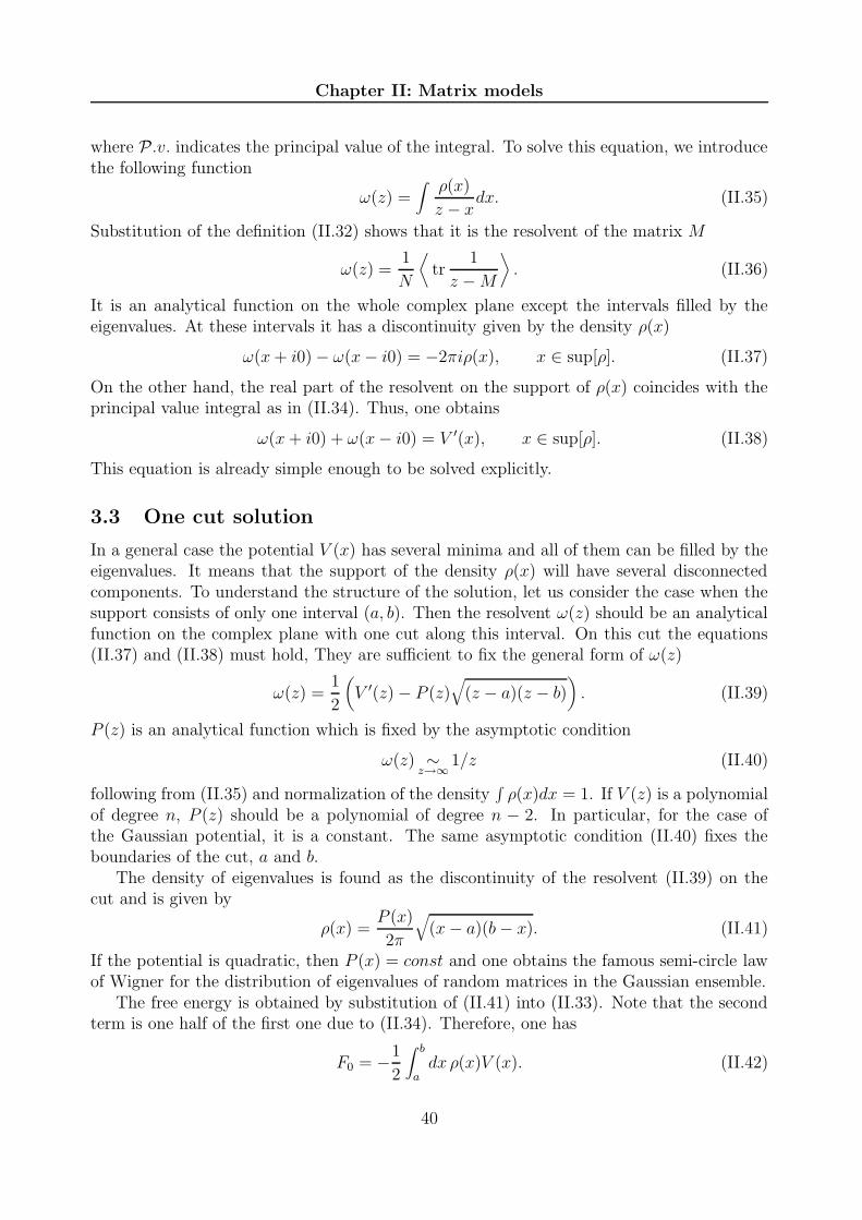
Chapter II: Matrix models
where P.v. indicates the principal value of the integral. To solve this equation, we introducethe following function
ω(z) =∫
ρ(x)
z − xdx. (II.35)
Substitution of the definition (II.32) shows that it is the resolvent of the matrix M
ω(z) =1
N
⟨
tr1
z −M
⟩
. (II.36)
It is an analytical function on the whole complex plane except the intervals filled by theeigenvalues. At these intervals it has a discontinuity given by the density ρ(x)
ω(x+ i0) − ω(x− i0) = −2πiρ(x), x ∈ sup[ρ]. (II.37)
On the other hand, the real part of the resolvent on the support of ρ(x) coincides with theprincipal value integral as in (II.34). Thus, one obtains
ω(x+ i0) + ω(x− i0) = V ′(x), x ∈ sup[ρ]. (II.38)
This equation is already simple enough to be solved explicitly.
3.3 One cut solution
In a general case the potential V (x) has several minima and all of them can be filled by theeigenvalues. It means that the support of the density ρ(x) will have several disconnectedcomponents. To understand the structure of the solution, let us consider the case when thesupport consists of only one interval (a, b). Then the resolvent ω(z) should be an analyticalfunction on the complex plane with one cut along this interval. On this cut the equations(II.37) and (II.38) must hold, They are sufficient to fix the general form of ω(z)
ω(z) =1
2
(
V ′(z) − P (z)√
(z − a)(z − b))
. (II.39)
P (z) is an analytical function which is fixed by the asymptotic condition
ω(z) ∼z→∞
1/z (II.40)
following from (II.35) and normalization of the density∫
ρ(x)dx = 1. If V (z) is a polynomialof degree n, P (z) should be a polynomial of degree n − 2. In particular, for the case ofthe Gaussian potential, it is a constant. The same asymptotic condition (II.40) fixes theboundaries of the cut, a and b.
The density of eigenvalues is found as the discontinuity of the resolvent (II.39) on thecut and is given by
ρ(x) =P (x)
2π
√
(x− a)(b− x). (II.41)
If the potential is quadratic, then P (x) = const and one obtains the famous semi-circle lawof Wigner for the distribution of eigenvalues of random matrices in the Gaussian ensemble.
The free energy is obtained by substitution of (II.41) into (II.33). Note that the secondterm is one half of the first one due to (II.34). Therefore, one has
F0 = −1
2
∫ b
adx ρ(x)V (x). (II.42)
40

§3 One-matrix model: saddle point approach
V
xa b
Fig. II.4: Critical point in one-matrix model.
3.4 Critical behaviour
The result (II.41) shows that near the end of the support the density of eigenvalues doesnot depend on the potential and always behaves as a square root. This is a manifestation ofuniversality of matrix models mentioned in the end of section 2.
However, there are degenerate cases when this behaviour is violated. This can happenif the polynomial P (x) vanishes at x = a or x = b. For example, if a is a root of M(x) ofdegree m, the density behaves as ρ(x) ∼ (x − a)m+1/2 near this point. It is clear that thissituation is realized only for special values of the coupling constants gk. They correspondto the critical points of the free energy discussed in connection with the continuum limit inparagraph 2.5. Indeed, one can show that near these configurations the spherical free energy(II.42) looks as (II.19) with χ = 2 and γstr = −1/(m+ 1) [58, 60].
Thus, each critical point with a given m defines a class of universality. All these classescorrespond to continuum theories which are associated with special discrete series of CFTsliving on dynamical surfaces. This discrete series is a part of the so called minimal conformal
theories which possess only finite number of primary fields [61]. The minimal CFTs arecharacterized by two relatively prime integers p and q with the following central charge andstring susceptibility
c = 1 − 6(p− q)2
pq, γstr = − 2
p + q − 1. (II.43)
Our case is obtained when p = 2m + 1, q = 2. Thus, for m = 1 the central charge vanishesand we describe the pure two-dimensional quantum gravity. The critical points with otherm describe the two-dimensional quantum gravity coupled to the matter characterized by the
rational central charge c = 1 − 3 (2m−1)2
2m+1.
From the matrix model point of view, there is a clear interpretation for the appearanceof the critical points. Usually, in the large N limit the matrix eigenvalues fill consecutivelythe lowest energy levels in the well around a minimum of the effective potential. The criticalbehaviour arises when the highest filled level reaches an extremum of the effective potential.Generically, this happens as shown in fig. II.4. By fine tuning of the coupling constants, onecan get more special configurations which will describe the critical behaviour with m > 1.
41
Chapter II: Matrix models
B1
BA
z1A
kk
Fig. II.5: Riemann surface associated with the solution of 1MM.
3.5 General solution and complex curve
So far we considered the case where the density is concentrated on one interval. The generalform of the solution can be obtained if we note that equation (II.38) can be rewritten as thefollowing equation valid in the whole complex plane
y2(z) = Q(ζ), y = ω(z) − 1
2V ′(z), (II.44)
where Q(z) is some analytical function. Its form is fixed by the condition (II.40) which leadsto Q(z) = V ′2(z) + Q(z), where Q(z) is a polynomial of degree n − 2. Thus, the solutionreads
y(z) =√
V ′2(z) +Q(z). (II.45)
In a general case, the polynomial Q(z) has 2(n− 1) roots so that the solution is
y(z) =
√
√
√
√
n−1∏
k=1
(z − ak)(z − bk), (II.46)
where we imply the ordering a1 < b1 < a2 < . . . < bn−1. The intervals (ak, bk) represent thesupport of the density. When ak coincides with bk, the corresponding interval collapses andwe get a factor (z−ak) in front of the square root. When n−2 intervals collapse, we return tothe one cut solution (II.39). Note that at the formal level the eigenvalues can appear aroundeach extremum, not only around minima, of the potential. However, the condensation of theeigenvalues around maxima is not physical and cannot be realized as a stable configuration.
Thus, we see that the solution of 1MM in the large N limit is completely determined bythe resolvent ω(z) whose general structure is given in (II.45). It is an analytical functionwith at most n − 1 cuts having the square root structure. Therefore one can consider aRiemann surface associated with this function. It consists from two sheets joint by all cuts(fig. II.5). Similarly, it can be viewed as a genus nc complex curve where nc is the numberof cuts.
On such curve there are 2nc independent cycles. nc compact cycles Ak go around cuts andnc non-compact cycles Bk join cuts with infinity. The integrals of a holomorphic differential
42

§3 One-matrix model: saddle point approach
along these cycles can be considered as the moduli of the curve. In our case the role of suchdifferential is played by y(z)dz. From the definition (II.44) it is clear that the integrals alongthe cycles Ak give the relative numbers of eigenvalues in each cut
1
2πi
∮
Ak
y(z)dz =∫ bk
ak
ρ(x)dxdef= nk. (II.47)
By definition∑nck=1 nk = 1. The integrals along the cycles Bk can also be calculated and are
given by the derivatives of the free energy [62, 63]
∫
Bk
y(z)dz =∂F0
∂nk. (II.48)
Thus, the solution of the one-matrix model in the large N limit is encoded in the complexstructure of the Riemann surface associated with the resolvent of the matrix.
43

Chapter II: Matrix models
4 Two-matrix model: method of orthogonal polyno-
mials
In this section we consider the two-matrix model (II.7) which describes the Ising model on arandom lattice. We restrict ourselves to the simplest case of the potential of the type (II.9).Thus, we are interested in the following integral over two hermitian matrices
Z =∫
dA dB exp[
−N tr(
AB − V (A) − V (B))]
, (II.49)
where the potentials V (A) and V (B) are some polynomials and the measures are the same asin (II.24). We will solve this model by the method of orthogonal polynomials. This approachcan be also applied to 1MM where it looks even simpler. However, we would like to illustratethe basic features of 2MM and the technique of orthogonal polynomials is quite convenientfor this.
4.1 Reduction to eigenvalues
Similarly to the one-matrix case, one can diagonalize the matrices and rewrite the integralin terms of their eigenvalues. However, now one has to use two unitary matrices, which arein general different, for the diagonalization
A = Ω†AxΩA, B = Ω†
ByΩB. (II.50)
At the same time, the action in (II.49) is invariant only under the common unitary transfor-mation (II.8). Therefore, only one of the two unitary matrices is canceled. As a result, onearrives at the following representation
Z = CN
∫ N∏
k=1
dxk dyk eN(V (xk)+V (yk))∆2(x)∆2(y)I(x, y), (II.51)
whereI(x, y) =
∫
[dΩ]SU(N) exp[
−N tr(
Ω†xΩy)]
(II.52)
and Ω = ΩAΩ†B . The integral (II.52) is known as Itzykson–Zuber–Charish-Chandra integral
and can be calculated explicitly [64]
I(x, y) = CNdet e−Nxiyj
∆(x)∆(y), (II.53)
where CN is some constant. Substitution of this result into (II.51) leads to the cancellationof a half of the Vandermonde determinants. The remaining determinants make the inte-gration measure antisymmetric under permutations xk and yk. Due to this antisymmetry,the determinant det eNxiyj can be replaced by the the product of diagonal terms. The finalresult reads
Z = C ′N
∫ N∏
k=1
dµ(xk, yk) ∆(x)∆(y), (II.54)
where we introduced the measure
dµ(x, y) = dx dy e−N(xy−V (x)−V (y)). (II.55)
44

§4 Two-matrix model: method of orthogonal polynomials
4.2 Orthogonal polynomials
Let us introduce the system of polynomials orthogonal with respect to the measure (II.55)∫
dµ(x, y)Φn(x)Φm(y) = δnm. (II.56)
It is easy to check that they are given by the following expressions
Φn(x) =1
n!√hn
∫ n∏
k=1
dµ(xk, yk)
hk−1∆(x)∆(y)
n∏
k=1
(x− xk), (II.57)
Φn(y) =1
n!√hn
∫ n∏
k=1
dµ(xk, yk)
hk−1
∆(x)∆(y)n∏
k=1
(y − yk), (II.58)
where the coefficients hn are fixed by the normalization condition in (II.56). They can becalculated recursively by the relation
hn =1
(n+ 1)!
(
n∏
k=1
hk−1
)−1∫ n+1∏
k=1
dµ(xk, yk)∆(x)∆(y). (II.59)
Due to this, the general form of the polynomials is the following
Φn(x) =1√hnxn +
n−1∑
k=0
cn,kxk, (II.60)
Φn(y) =1√hnyn +
n−1∑
k=0
dn,kyk. (II.61)
Using these polynomials, one can rewrite the partition function (II.54). Indeed, due tothe antisymmetry the Vandermonde determinants (II.28) can be replaced by determinantsof the orthogonal polynomials multiplied by the product of the normalization coefficients.Then one can apply the orthonormality relation (II.56) so that
Z = C ′N
(
N−1∏
k=0
hk
)
∫ N∏
k=1
dµ(xk, yk) detij
(Φj−1(xi)) detij
(
Φj−1(yi))
= C ′NN !
N−1∏
k=0
hk. (II.62)
Thus, we reduced the problem of calculation of the partition function to the problem offinding the orthogonal polynomials and their normalization coefficients.
4.3 Recursion relations
To find the coefficients hn, cn,k and dn,k of the orthogonal polynomials, one uses recursionsrelations which can be obtained for Φn and Φn. They are derived using two pairs of conju-gated operators which are the operators of multiplication and derivative [65]. We introducethem as the following matrices representing these operators in the basis of the orthogonalpolynomials
xΦn(x) =∑
mXnmΦm(x), 1
N∂∂x
Φn(x) =∑
mPnmΦm(x), (II.63)
yΦn(y) =∑
mΦm(y)Ymn,
1N
∂∂y
Φn(y) =∑
mΦm(y)Qmn. (II.64)
45

Chapter II: Matrix models
Integrating by parts, one finds the following relations
Pnm = Ynm − [V ′(X)]nm, Qnm = Xnm − [V ′(Y )]nm. (II.65)
If one takes the potentials V (x) and V (y) of degree p and q, correspondingly, the form of theorthogonal polynomials (II.60), (II.61) and relations (II.65) imply the following properties
Xn,n+1 = Yn+1,n =√
hn+1/hn,
Xnm = 0, m > n + 1 and m < n− q + 1,Ymn = 0, m > n+ 1 and m < n− p+ 1,
Pn,n−1 = Qn−1,n = nN
√
hn−1/hn,
Pnm = Qnm = 0, m > n− 1 and m < n− (p− 1)(q − 1).
(II.66)
They indicate that it is more convenient to work with redefined indices
Xk(n/N) = Xn,n−k, Yk(n/N) = Yn−k,n (II.67)
and similarly for P and Q. Then each set of functions can be organized into one operatoras follows
X(s) =q−1∑
k=−1Xk(s)ω
−k, P (s) =(p−1)(q−1)
∑
k=1Pk(s)ω
−k, (II.68)
Y (s) =p−1∑
k=−1ωkYk(s), Q(s) =
(p−1)(q−1)∑
k=1ωkQk(s), (II.69)
where we denoted s = n/N and introduced the shift operator ω = e1N
∂∂s . These operators
satisfy
X(n/N)Φn(x) = xΦn(x), P (n/N)Φn(x) = 1N
∂∂x
Φn(x), (II.70)
Y †(n/N)Φn(x) = yΦn(y), Q†(n/N)Φn(y) = 1N
∂∂y
Φn(y), (II.71)
where the conjugation is defined as (ωa(s))† = a(s)ω−1. With these definitions the relations(II.65) become
P (s) = Y (s) − V ′(X(s)), Q(s) = X(s) − V ′(Y (s)). (II.72)
Substitution of the expansions (II.68) and (II.69) into (II.72) gives a system of finite-difference algebraic equations, which are obtained comparing the coefficients in front ofpowers of ω. Actually, one can restrict the attention only to negative powers. Then thereduced system contains only equations on the functions Xk and Yk, because the left handside of (II.72) is expanded only in positive powers of ω. This is a triangular system andfor each given potential it can be solved by a recursive procedure. The free energy can be
reproduced from the function Rn+1def= X2
−1(n/N) = Y 2−1(n/N). The representation (II.62)
implies
Z = C ′NN !
N−1∏
k=0
RN−kk . (II.73)
46

§4 Two-matrix model: method of orthogonal polynomials
This gives the solution for all genera.In fact, to find the solution of (II.72), one has to use the perturbative expansion in 1/N .
Then the problem is reduced to a hierarchy of differential equations. The hierarchy appearinghere is Toda lattice hierarchy which will be described in detail in the next section. The useof methods of Toda theory simplifies the problem and allows to find explicit differential, andeven algebraic equations directly for the free energy.
4.4 Critical behaviour
We saw in section 3.4 that the multicritical points of the one-matrix model correspond toa one-parameter family of the minimal conformal theories. The two-matrix model is moregeneral than the one-matrix model. Therefore, it can encompass a larger class of continuousmodels. It turns out that all minimal models (II.43) can be obtained by appropriatelyadjusting the matrix model potentials [65, 66].
There is an infinite set of critical potentials for each (p, q) point. The simplest one is whenone of the potentials has degree p and the other has degree q. Their explicit form has beenconstructed in [66]. The key fact of the construction is that the momentum function P (ω, s)(up to an analytical piece) is identified with the resolvent (II.36) of the corresponding matrixX. Comparing with the one-matrix case, one concludes that the (p, q) point is obtained whenthe resolvent behaves near its singularity as (x − xc)
p/q. Thus, it is sufficient to take theoperators with the following behaviour at ω → 1
X −Xc ∼ (logω)q, P − Pc ∼ (logω)p. (II.74)
Note that the singular asymptotics of Y and Q follow from (II.72) and lead to the dual (q, p)point. Then one can take some fixed X(w) and Y (w) with the necessary asymptotics atω → 1 and ω → ∞ and solve the equations (II.72) with respect to the potentials V (X) andV (Y ). The resulting explicit formulae can be found in [66].
4.5 Complex curve
As in the one-matrix model, the solution of 2MM in the large N limit can be represented interms of a complex curve [67, 68]. However, there is a difference between these two cases.Whereas in the former case the curve coincides with the Riemann surface of the resolvent,in the latter case the origin of the curve is different. To illuminate it, let us consider howthe solution of the model in the large N limit arises.
In this approximation one can apply the saddle point approach described in the previoussection. It leads to the following two equations on the resolvents of matrices X and Y
y = V ′(x) + ω(x), x = V ′(y) + ω(y). (II.75)
In fact, these equations are nothing else but the classical limit of the relations (II.72) obtainedusing the orthogonal polynomials. They coincide due to the identification mentioned aboveof the momentum operators P and Q with the resolvents ω and ω, respectively.
The equations (II.75) can be considered as definitions of the multivalued analytical func-tions y(x) and x(y). It is clear that they must be mutually inverse. This is actually a
47

Chapter II: Matrix models
P1 +
−
P1
n
12 n
1
2
Fig. II.6: Generic curve of 2MM as a cover of x-plane. Each fat line consists from n cuts.
( ) x ρ
( ) yρ
y
x
Fig. II.7: Eigenvalue plane of 2MM. The eigenvalues fill several spots which contain infor-mation about the density.
non-trivial restriction which, together with the asymptotic condition (II.40), fixes the re-solvents and gives the solution. The complex curve, one should deal with, is the Riemannsurface of one of these functions.
The general structure of this complex curve was studied in [68]. It was established thatif the potentials are of degree n + 1 and n + 1, the maximum genus of the curve is nn − 1.In this most general case the Riemann surface is represented by n + 1 sheets. One of themis the ”physical sheet” glued with each ”unphysical” one along n cuts and all ”unphysicalsheets” join at infinity by the nth order branch point (see fig. II.6).
One can prove the analog of the formulae (II.47) and (II.48) [68]. We still integratearound two conjugated sets of independent cycles Ak and Bk on the curve. The role of theholomorphic differential is played again by y(z)dz where y(x) is a solution of (II.75).
As earlier, the cycles Ak surround the cuts of the resolvent on the physical sheet. This isthe place where the eigenvalues of the matrix X live. However, in this picture it is not clearhow to describe the distribution of eigenvalues of Y . Of course, it is enough to invert thefunction y(x) to find it. But the arising picture is nevertheless non-symmetric with respect
48

§4 Two-matrix model: method of orthogonal polynomials
Ak
kB
Fig. II.8: Complex curve associated with the solution of 2MM viewed as a ”double” of(x, y)-plane.
to the exchange of x and y.
A more symmetric picture can be obtained considering the so called ”double” [68]. Tointroduce this notion, note that since the two matrices X and Y are of the same size,with each eigenvalue xi one can associate an eigenvalue yi of the second matrix. Thus, oneobtains N pairs (xi, yi) which can be put on a plane. In the large N limit, the eigenvaluesare distributed continuously so that on the plane (x, y) their distribution appears as severaldisconnected regions. Each region corresponds to a cut of the resolvent. Its width in they direction at a given point x is nothing else but the density ρ(x) and vice versa. Thus,one arrives at a two-dimensional picture shown on fig. II.7. From this point of view, thefunctions y(x) and x(y), which are solutions of (II.75), determine the boundaries of the spotsof eigenvalues. The fact that they are inverse means that they define the same boundary.
Now to define the double, we take two copies of the (x, y) plane, cut off the spots, andglue them along the boundaries. The resulting surface shown in fig. II.8 is smooth and canbe considered as a genus nc− 1 surface with two punctures (corresponding to two infinities)where nc is the number of spots on the initial surface equal to the number of cuts of theresolvent ω(x).
All cycles Ak and Bk exist also in this picture and the integration formulae (II.47) and(II.48) along them hold as well. Note that the integrals along Ak cycles can be rewritten astwo-dimensional integrals over the (x, y) plane with the density equal to 1 inside the spotsand vanishing outside them. Such behaviour of the density is characteristic for fermionicsystems. And indeed, 2MM can be interpreted as a system of free fermions.
4.6 Free fermion representation
Let us identify the functions
ψn(x) = Φn(x)eNV (x), ψn(y) = Φn(y)e
NV (y). (II.76)
49

Chapter II: Matrix models
with fermionic wave functions. The functions ψn and ψn can be considered as two representa-tions of the same state similarly to the coordinate and momentum representations. The tworepresentations are related by a kind of Fourier transform and the scalar product betweenfunctions of different representations is given by the following integral
⟨
ψ|ψ⟩
=∫
dx dy e−Nxyψ(y)ψ(x). (II.77)
The second-quantized fermionic fields are defined as
ψ(x) =∞∑
n=0
anψn(x), ψ(y) =∞∑
n=0
a†nψn(y). (II.78)
Due to the orthonormality of the wave functions (II.76) with respect to the scalar prod-uct (II.77), the creation and annihilation operators satisfy the following anticommutationrelations
an, a†m = δn,m. (II.79)
The fundamental state of N fermions is defined by
an|N〉 = 0, n ≥ N, a†n|N〉 = 0, n < N. (II.80)
Its wave function can be represented by the Slater determinant. For example, in the x-representation it looks as
ΨN (x1, . . . , xN ) = deti,j
ψi(xj). (II.81)
The key observation which establishes the equivalence of the two systems is that the cor-relators of matrix operators coincide with expectation values of the corresponding fermionicoperators in the fundamental state (II.81):
⟨
∏
j
trBmj∏
i
trAni
⟩
=
⟨
N |∏
j
ymj∏
i
xni|N⟩
. (II.82)
Here a second-quantized operator O(x, y) is defined as follows
O(x, y) =∫
dx dy e−Nxyψ(y)O(x, y)ψ(x). (II.83)
The proof of the statement (II.82) relies on the properties of the orthogonal polynomials.For example, for the one-point correlator we have
〈 trAn〉 ≡ Z−1∫
dA dB trAn e−N tr (AB−V (A)−V (B))
=
(
N !N−1∏
k=0
hk
)−1∫ N∏
k=1
dµ(xk, yk) ∆(x)∆(y)N∑
i=1
xni
=1
(N − 1)!
∫ N∏
k=1
dµ(xk, yk) detij
(Φj−1(xi)) detij
(
Φj−1(yi))
xn1
=N−1∑
j=0
∫
dµ(x, y) Φj(x)Φj(y)xn = 〈N |xn|N〉 . (II.84)
50

§4 Two-matrix model: method of orthogonal polynomials
This equivalence supplies us with a powerful technique for calculations. For example, allcorrelators of the type (II.82) can be expressed through the two-point function
KN(x, y) =⟨
N |ψ(y)ψ(x)|N⟩
(II.85)
and it is sufficient to study this quantity. In general, the existence of the representation interms of free fermions indicates that the system is integrable. This, in turn, is often relatedto the possibility to introduce orthogonal polynomials.
We will see that the similar structures appear in matrix quantum mechanics. AlthoughMQM has much richer physics, it turns out to be quite similar to 2MM.
51

Chapter II: Matrix models
5 Toda lattice hierarchy
5.1 Integrable systems
One and two-matrix models considered above are examples of integrable systems. Thereexists a general theory of such systems. A system is considered as integrable if it has aninfinite number of commuting Hamiltonians. Each Hamiltonian generates an evolution alongsome direction in the parameter space of the model. Their commutativity means that thereis an infinite number of conserved quantities associated with them and, at least in principle,it is possible to describe any point in the parameter space.
Usually, the integrability implies the existence of a hierarchy of equations on some specificquantities characterizing the system. The hierarchical structure means that the equationscan be solved one by one, so that the solution of the first equation should be substitutedinto the second one and etc. This recursive procedure allows to reproduce all informationabout the system.
The equations to be solved are most often of the finite-difference type. In other words,they describe a system on a lattice. Introducing a parameter measuring the spacing betweennodes of the lattice, one can organize a perturbative expansion in this parameter. Thenthe finite-difference equations are replaced by an infinite set of partial differential equations.They also form a hierarchy and can be solved recursively. The equations appearing atthe first level, corresponding to the vanishing spacing, describe a closed system which isconsidered as a continuum or classical limit of the initial one. In turn, starting with theclassical system describing by a hierarchy of differential equations, one can construct itsquantum deformation arriving at the full hierarchy.
The integrable systems can be classified according to the type of hierarchy which appearsin their description. In this section we consider the so called Toda hierarchy [69]. It isgeneral enough to include all integrable matrix models relevant for our work. In particular,it describes 2MM and some restriction of MQM, whereas 1MM corresponds to its certainreduction.
5.2 Lax formalism
There are several ways to introduce the Toda hierarchy. The most convenient for us is touse the so called Lax formalism.
Take two semi-infinite series1
L = r(s)ω +∞∑
k=0
uk(s)ω−k, L = ω−1r(s) +
∞∑
k=0
ωkuk(s), (II.86)
where s is a discrete variable labeling the nodes of an infinite lattice and ω = eh∂/∂s is theshift operator in s. The Planck constant h plays the role of the spacing parameter. The
1In fact, the first coefficients in the expansions (II.86) can be chosen arbitrarily. Only their product hasa sense and how it is distributed between the two operators can be considered as a choice of some gauge. Inparticular, often one uses the gauge where one of the coefficients equals 1 [70]. We use the symmetric gaugewhich agrees with the choice of the orthogonal polynomials (II.56) normalized to the Kronecker symbol in2MM.
52

§5 Toda lattice hierarchy
operators (II.86) are called Lax operators. The coefficients r, uk and uk are also functions oftwo infinite sets of ”times” t±k∞k=1. Each time variable gives rise to an evolution along itsdirection. This system represents Toda hierarchy if the evolution associated with each t±kis generated by Hamiltonians H±k
h ∂L∂tk
= [Hk, L], h ∂L∂tk
= [Hk, L],
h ∂L∂t−k
= [H−k, L], h ∂L∂t−k
= [H−k, L],(II.87)
which are expressed through the Lax operators (II.86) as follows2
Hk = (Lk)+ +1
2(Lk)0, H−k = (Lk)− +
1
2(Lk)0, (II.88)
where the symbol ( )><
means the positive (negative) part of the series in the shift operator
ω and ( )0 denotes the constant part. Thus, Toda hierarchy is a collection of non-linearequations of the finite-difference type in s and differential with respect to tk for the coefficientsr(s, t), uk(s, t) and uk(s, t).
From the commutativity of the second derivatives, it is easy to obtain that the Lax–Satoequations (II.87) are equivalent to the zero-curvature condition for the Hamiltonians
h∂Hk
∂tl− h
∂Hl
∂tk+ [Hk, Hl] = 0. (II.89)
It shows that the system possesses an infinite set of commutative flows h ∂∂tk
− Hk and,therefore, Toda hierarchy is integrable.
One can get another equivalent formulation if one considers the following eigenvalueproblem
xΨ = LΨ(x; s), h∂Ψ
∂tk= HkΨ(x; s), h
∂Ψ
∂t−k= H−kΨ(x; s). (II.90)
The previous equations (II.87) and (II.89) appear as the integrability condition for (II.90).Indeed, differentiating the first equation, one reproduces the evolution law of the Lax opera-tors (II.87) and the second and third equations lead to the zero-curvature condition (II.89).The eigenfunction Ψ is known as Baker–Akhiezer function. It is clear that it contains allinformation about the system.
Note that equations of Toda hierarchy allow a representation in terms of semi-infinitematrices. Then the Baker–Akhiezer function is a vector whose elements correspond to dif-ferent values of the discrete variable s. The positive/negative/constant parts of the series inω are mapped to upper/lower/diagonal triangular parts of matrices.
The equations to be solved are either the equations (II.90) on Ψ or the Lax–Sato equations(II.87) on the coefficients of the Lax operators. Their hierarchic structure is reflected inthe fact that one obtains a closed equation on the first coefficient r(s, t) and its solution
2 Sometimes the second set of Hamiltonians is defined with the opposite sign. This corresponds to thechange of sign of t−k. Doing both these replacements, one can establish the full correspondence with theworks using this sign convention.
53

Chapter II: Matrix models
provides the necessary information for the following equations. This first equation is derivedconsidering the Lax–Sato equations (II.87) for k = 1. They give
h∂ log r2(s)∂t1
= u0(s+ h) − u0(s), h∂ log r2(s)∂t−1
= u0(s) − u0(s+ h), (II.91)
h∂u0(s)∂t1
= r2(s) − r2(s− h), h∂u0(s)∂t−1
= r2(s− h) − r2(s). (II.92)
Combining these relations, one finds the so called Toda equation
h2∂2 log r2(s)
∂t1∂−1= 2r2(s) − r2(s+ h) − r2(s− h). (II.93)
Often it is convenient to introduce the following Orlov–Shulman operators [71]
M =∑
k≥1ktkL
k + s+∑
k≥1vkL
−k,
M = − ∑
k≥1kt−kL
k + s− ∑
k≥1v−kL
−k.(II.94)
The coefficients v±k are fixed by the condition on their commutators with the Lax operators
[L,M ] = hL, [L, M ] = −hL. (II.95)
The main application of these operators is that they can be considered as perturbations ofthe simple operators of multiplication by the discrete variable s. Indeed, if one requires thatv±k vanish when all t±k = 0, then in this limit M = M = s. Similarly the Lax operatorsreduce to the shift operator. The perturbation leading to the general expansions (II.86) and(II.94) can be described by the dressing operators W and W
L = WωW−1, M = WsW−1,L = Wω−1W−1, M = WsW−1.
(II.96)
The commutation relations (II.95) are nothing else but the dressed version of the evidentrelation
[ω, s] = hω. (II.97)
To produce the expansions (II.86) and (II.94), the dressing operators should have thefollowing general form
W = e12hφ
(
1 +∑
k≥1wkω
−k)
exp
(
1h
∑
k≥1tkω
k
)
,
W = e−12hφ
(
1 +∑
k≥1wkω
k
)
exp
(
1h
∑
k≥1t−kω
−k)
,
(II.98)
where the zero mode φ(s) is related to the coefficient r(s) as
r2(s) = e1h(φ(s)−φ(s+h)). (II.99)
However, the coefficients in this expansion are not arbitrary and the dressing operators shouldbe subject of some additional condition. It can be understood considering evolution along
54

§5 Toda lattice hierarchy
the times t±k. Differentiating (II.96) with respect to t±k, one finds the following expressionof the Hamiltonians in terms of the dressing operators
Hk = h(∂tkW)W−1, H−k = h(∂t−kW)W−1,
Hk = h(∂tkW)W−1, H−k = h(∂t−kW)W−1,
(II.100)
Here H±k generate evolution of L and H±k are Hamiltonians for L. However, (II.87) impliesthat for both operators one should use the same Hamiltonian. This imposes the conditionthat H±k = H±k which relates two dressing operators. This condition can be rewritten in amore explicit way. Namely, it is equivalent to the requirement that W−1W does not dependon times t±k [69, 72].
Studying the evolution laws of the Orlov–Shulman operators, one can find that [70]
∂vk∂tl
=∂vl∂tk
. (II.101)
It means that there exists a generating function τs[t] of all coefficients v±k
vk(s) = h2 ∂ log τs[t]
∂tk. (II.102)
It is called τ -function of Toda hierarchy. It also allows to reproduce the zero mode φ and,consequently, the first coefficient in the expansion of the Lax operators
e1hφ(s) =
τsτs+h
, r2(s− h) =τs+hτs−h
τ 2s
. (II.103)
The τ -function is usually the main subject of interest in the systems described by Todahierarchy. The reason is that it coincides with the partition function of the model. Thenthe coefficients vk are the one-point correlators of the operators generating the commutingflows Hk. We will show a concrete realization of these ideas in the end of this section and inthe next chapters.
5.3 Free fermion and boson representations
To establish an explicit connection with physical systems, it is sometimes convenient to use arepresentation of Toda hierarchy in terms of second-quantized free chiral fermions or bosons.The two representations are related by the usual bosonization procedure.
Fermionic picture
To define the fermionic representation, let us consider the chiral fermionic fields with thefollowing expansion
ψ(z) =∑
r∈Z+ 12
ψrz−r− 1
2 , ψ∗(z) =∑
r∈Z+ 12
ψ∗−rz
−r− 12 (II.104)
Their two-point function
〈l|ψ(z)ψ∗(z′)|l〉 =(z′/z)l
z − z′(II.105)
55

Chapter II: Matrix models
leads to the following commutation relations for the modes
ψr, ψ∗s = δr,s. (II.106)
The fermionic vacuum of charge l is defined by
ψr|l〉 = 0, r > l, ψ∗r |l〉 = 0, r < l. (II.107)
Also we need to introduce the current
J(z) = ψ∗(z)ψ(z) = pz−1 +∑
n6=0
Hnz−n−1 (II.108)
whose components Hn are associated with the Hamiltonians generating the Toda flows. Interms of the fermionic modes they are represented as follows
Hn =∑
r∈Z+ 12
ψ∗r−nψr (II.109)
and for any l they satisfyHn|l〉 = 〈l|H−n = 0, n > 0. (II.110)
Finally, we introduce an operator of GL(∞) rotation
g = exp
1
h
∑
r,s∈Z+ 12
Arsψrψ∗s
. (II.111)
With these definitions the τ -function of Toda hierarchy is represented as the followingvacuum expectation value
τlh[t] =⟨
l|e 1hH+[t]ge−
1hH−[t]|l
⟩
, (II.112)
whereH+[t] =
∑
k>0
tkHk, H−[t] =∑
k<0
tkHk. (II.113)
It is clear that each solution of Toda hierarchy is characterized in the unique way by thechoice of the matrix Ars.
Bosonic picture
The bosonic representation now follows from the bosonization formulae
ψ(z) =: eϕ(z) :, ψ∗(z) =: e−ϕ(z) :, ∂ϕ(z) =: ψ∗(z)ψ(z) : . (II.114)
Since the last expression in (II.114) is the current (II.108), the Hamiltonians Hn appear nowas the coefficients in the mode expansion of the free bosonic field
ϕ(z) = q + p log z +∑
n6=0
1
nHnz
−n. (II.115)
56

§5 Toda lattice hierarchy
From (II.109) and (II.106) one finds the following commutation relations
[p, q] = 1, [Hn, Hm] = nδm+n,0, (II.116)
which lead to the two-point function of the free boson
〈ϕ(z)ϕ(z′)〉 = log(z − z′). (II.117)
The bosonic vacuum is defined by the Hamiltonians and characterized by the quantumnumber s, which is the eigenvalue of the momentum operator,
p|s〉 = s|s〉, Hn|s〉 = 0, (n > 0). (II.118)
To rewrite the operator g (II.111) in the bosonic terms, we introduce the vertex operators
Vα(z) =: eαϕ(z) : . (II.119)
Here the normal ordering is defined by putting all Hn, n > 0 to the right and Hn, n < 0 tothe left. Besides : qp :=: pq := qp. Then the operator of GL(∞) rotation is given by
g = exp(
− 1
4π2h
∮
dz∮
dwA(z, w)V1(z)V−1(w))
, (II.120)
whereA(z, w) =
∑
r,s
Arszr− 1
2w−s− 12 . (II.121)
The substitution of (II.120) into (II.112) and replacing the fermionic vacuum |l〉 by thebosonic one |s〉 gives the bosonic representation of the τ -function τs[t].
Connection with the Lax formalism
The relation of these two representations with the objects considered in paragraph 5.2 isbased on the realization of the Baker–Akhiezer function Ψ(z; s) as the expectation value ofthe one-fermion field
Ψ(z; s) = τ−1s [t]
⟨
h−1s|e 1hH+[t]ψ(z)ge−
1hH−[t]|h−1s
⟩
. (II.122)
One can show that it does satisfy the relations (II.90) with Hk defined as in (II.88) and theLax operators having the form (II.86).
5.4 Hirota equations
The most explicit manifestation of the hierarchic structure of the Toda system is a setof equations on the τ -function, which can be obtained from the fermionic representationintroduced above. One can show [73] that the ensemble of the τ -functions of the Todahierarchy with different charges satisfies a set of bilinear equations. They are known asHirota equations and can be written in a combined way as follows
∮
C∞ dz zl−l′exp
(
1h
∑
k>0(tk − t′k)z
k
)
τl[t− ζ+]τl′ [t′ + ζ+] =
∮
C0dz zl−l
′exp
(
1h
∑
k<0(tk − t′k)z
k
)
τl+1[t− ζ−]τl′−1[t′ + ζ−], (II.123)
57

Chapter II: Matrix models
where
ζ+/h = (. . . , 0, 0, z−1, z−2/2, z−3/3, . . .), ζ−/h = (. . . , z3/3, z2/2, z, 0, 0, . . .) (II.124)
and we omitted h in the index of the τ -function. The proof of (II.123) relies on the represen-tation (II.112) of the τ -function with g taken from (II.111). The starting point is the factthat the following operator
C =∑
r∈Z+ 12
ψ∗r ⊗ ψr =
∮
dz
2πiψ∗(z) ⊗ ψ(z) (II.125)
plays the role of the Casimir operator for the diagonal subgroup of GL(∞) ⊗GL(∞). Thismeans that it commutes with the tensor product of two g operators
C (g ⊗ g) = (g ⊗ g) C. (II.126)
Multiplying this relation by 〈l+ 1|e 1hH+[t] ⊗ 〈l′ − 1|e 1
hH+[t′] from the left and by e−
1hH−[t]|l〉 ⊗
e−1hH−[t′]|l′〉 from the right, one can commute the fermion operators until they hit the left
(right) vacuum. The final result is obtained using the following relations
〈l + 1|e 1hH+[t]ψ∗(z)ge−
1hH−[t]|l〉 = zl exp
(
1h
∑
n>0tnz
n
)
⟨
l|e 1hH+[t−ζ+]ge−
1hH−[t]|l
⟩
,(II.127)
〈l + 1|e 1hH+[t]gψ∗(z)e−
1hH−[t]|l〉 = zl exp
(
1h
∑
n<0tnz
n
)
⟨
l + 1|e 1hH+[t]ge−
1hH−[t−ζ−]|l + 1
⟩
(II.128)
together with the similar relations for ψ(z). They can be proven in two steps. First, onecommutes the fermionic fields with the perturbing operators
e−1hH±[t]ψ∗(z)e
1hH±[t] = exp
(
− 1h
∑
n>0t±nz
±n)
ψ∗(z),
e1hH±[t]ψ(z)e−
1hH±[t] = exp
(
− 1h
∑
n>0t±nz
±n)
ψ(z).(II.129)
After this it remains to show that, for example, ψ∗(z)|l〉 = zle1hH−[ζ−]|l+1〉. The easiest way
to do it is to use the bosonization formulae (II.114) and (II.115).The identities (II.123) can be rewritten in a more explicit form. For this we introduce
the Schur polynomials pj defined by
∞∑
k=0
pk[t]xk = exp
( ∞∑
k=1
tnxn
)
(II.130)
and the following notations
y± = (y±1, y±2, y±3, . . .), (II.131)
D± = (D±1, D±2/2, D±3/3, . . .), (II.132)
58

§5 Toda lattice hierarchy
where D±n represent the Hirota’s bilinear operators
Dnf [t] · g[t] =∂
∂xf(tn + x)g(tn − x)
∣
∣
∣
∣
∣
x=0
. (II.133)
Then identifying yn = 12h
(t′n − tn), one obtains a hierarchy of partial differential equations
∞∑
j=0pj+i(−2y+)pj(hD+) exp
(
h∑
k 6=0ykDk
)
τl+i+1[t] · τl[t] =
∞∑
j=0pj−i(−2y−)pj(hD−) exp
(
h∑
k 6=0ykDk
)
τl+i[t] · τl+1[t]. (II.134)
The Hirota equations lead to a triangular system of nonlinear difference-differential equa-tions for the τ -function. Since the derivatives of the τ -function are identified with correlators,the Hirota equations are also equations for the correlators of operators generating the Todaflows. The first equation of the hierarchy is obtained by taking i = −1 and extracting thecoefficient in front of y−1
h2 τl∂2τl
∂t1∂t−1− h2 ∂τl
∂t1
∂τl∂t−1
+ τl+1τl−1 = 0. (II.135)
Rewriting this equations as
h2 ∂2 log τl∂t1∂t−1
+τl+1τl−1
τ 2l
= 0, (II.136)
one can recognize the Toda equation (II.93) if one takes into account the identification(II.103).
5.5 String equation
We considered above the general structure of the Toda hierarchy. However, the equations ofthe hierarchy, for example, the Hirota equations (II.134), have many solutions. A particularsolution is characterized by initial condition. The role of such condition can be played by thepartition function of a non-perturbed system. If one requires that it should be equal to theτ -function at vanishing times and coincides with the full τ -function after the perturbation,the perturbed partition function can be found by means of the hierarchy equations with thegiven initial condition.
However, the Toda equations involve partial differential equations of high orders and re-quire to know not only the τ -function at vanishing times but also its derivatives. Therefore,it is not always clear whether the non-perturbed function provides a sufficient initial infor-mation. Fortunately, there is another way to select a unique solution of Toda hierarchy. Ituses some equations on the operators, usually, the Lax and Orlov–Shulman operators. Thecorresponding equations are called string equations.
The string equations cannot be arbitrary because they should preserve the structure ofToda hierarchy. For example, if they are given by two equations of the following type
L = f(L,M), M = g(L,M), (II.137)
59
Chapter II: Matrix models
the operators defined by the functions f and g must satisfy
[f(ω, s), g(ω, s)] = −hf. (II.138)
This condition appears since L and M commute in the same way.The advantage of use of string equations is that they represent in a sense already a
partially integrated version of the hierarchy equations. For example, as we will see, insteadof differential equations of the second order, they produce algebraic and first order differentialequations and make the problem of finding the τ -function much simpler.
5.6 Dispersionless limit
The classical limit of Toda hierarchy is obtained in the limit where the parameter measuringthe lattice spacing vanishes. In our notations this parameter is the Planck constant h.Putting it to zero, as usual, one replaces all operators by functions. In particular, as in theusual quantum mechanical systems, the classical limit of the derivative operator is a variableconjugated to the variable with respect to which one differentiates. In other words, oneshould consider the phase space consisting from s and ω, which is the classical limit of theshift operator. The Poisson structure on this phase space is defined by the Poisson bracketinduced from (II.97)
ω, s = ω. (II.139)
All operators now become functions of s and ω and commutators are replaced by the corre-sponding Poisson brackets defined through (II.139).
All equations including the Lax–Sato equations (II.87), zero curvature condition (II.89),commutators with Orlov–Shulman operators (II.95) can be rewritten in the new terms. Thus,the general structure of Toda hierarchy is preserved although it becomes much simpler. Theresulting structure is called dispersionless Toda hierarchy and the classical limit is also knownas dispersionless limit.
As in the full theory, a solution of the dispersionless Toda hierarchy is completely char-acterized by a dispersionless τ -function. In fact, one should consider the free energy since itis the logarithm of the full τ -function that can be represented as a series in h
log τ =∑
n≥0
h−2+2nFn. (II.140)
Thus, the dispersionless limit is extracted as follows
F0 = limh→0
h2 log τ. (II.141)
The dispersionless free energy F0 satisfies the classical limit of Hirota equations (II.134) andselected from all solutions by the same string equations (II.137) as in the quantum case.
Since the evolution along the times tk is now generated by the Hamiltonians through thePoisson brackets, it can be seen as a canonical transformation in the phase space definedabove. This fact is reflected also in the commutation relations (II.95). Since the Lax andOrlov–Shulman operators are dressed versions of ω and s, correspondingly, and have the samePoisson brackets, one can say that the dispersionless Toda hierarchy describe a canonicaltransformation from the canonical pair (ω, s) to (L,M). The free energy F0 plays the roleof the generating function of this transformation.
60

§5 Toda lattice hierarchy
5.7 2MM as τ-function of Toda hierarchy
In this paragraph we show how all abstract ideas described above get a realization in the two-matrix model. Namely, we identify the partition function (II.54) with a particular τ -functionof Toda hierarchy. This can be done in two ways using either the fermionic representationor the Lax formalism and its connection with the orthogonal polynomials. However, thefermionic representation which arises in this case is not exactly the same as in paragraph5.3, although it still gives a τ -function of Toda hierarchy. The difference is that one shoulduse two types of fermions [74]. In fact, they can be reduced to the fermions appearing inthe fermionic representation of 2MM presented in section 4.6. They differ only by the basiswhich is used in the mode expansions (II.104) and (II.78).
We will use the approach based on the Lax formalism. Following this way, one shouldidentify the Lax operators in the matrix model and prove that they satisfy the Lax-Satoequations (II.87). Equivalently, one can obtain the Baker–Akhiezer function satisfying (II.90)where the Hamiltonians Hk are related to the Lax operators through (II.88).
First of all, the Lax operators coincide with the operators X and Y defined in (II.68)and (II.69). Due to the first equation in (II.66), the operators have the same expansion asrequired in (II.86) where the first coefficient is
r(nh) =√
hn+1/hn. (II.142)
The Baker–Akhiezer function is obtained as a semi-infinite vector constructed from thefunctions ψn(x) (II.76)
Ψ(x;nh) = Φn(x)eNV (x). (II.143)
Due to (II.70), LΨ = xΨ. Thus, it remains to consider the evolution of Ψ in the couplingconstants. We fix their normalization choosing the potentials as follows
V (x) =∑
n>0
tnxn, V (x) = −
∑
n>0
t−nyn. (II.144)
Then the differentiation of the orthogonality condition (II.56) with respect to the couplingconstants leads to the following evolution laws
1N∂Φn(x)∂tk
= −n−1∑
m=0(Xk)nmΦm(x) − 1
2(Xk)nnΦn(x),
1N∂Φn(x)∂t−k
=n−1∑
m=0(Y k)nmΦm(x) + 1
2(Y k)nnΦn(x).
(II.145)
Using these relations one finds
1
N
∂Ψ
∂tk= HkΨ,
1
N
∂Ψ
∂t−k= H−kΨ, (II.146)
where H±k are defined as in (II.88). As a result, if one identifies 1/N with h, one reproducesall equations for the Baker–Akhiezer function. This means that the dynamics of 2MM withrespect to the coupling constants is governed by Toda hierarchy.
Combining (II.103) and (II.142), one finds
hn =τn+1
τn. (II.147)
61

Chapter II: Matrix models
Then the representation (II.62) implies
Z(N) ∼ τNτ0. (II.148)
The factor τ0 does not depend on N and appears as a non-universal contribution to the freeenergy. Therefore, it can be neglected and, choosing the appropriate normalization, one canidentify the partition function of 2MM with the τ -function of Toda hierarchy
Z(N) = τN . (II.149)
Moreover, one can find string equations uniquely characterizing the τ -function. First, wenote that the Orlov–Shulman operators (II.94) are given by
M = X(
V ′(X) + P)
− h, M = Y(
V ′(Y ) + Q)
. (II.150)
Then the relations (II.72) imply
LL = M + h, LL = M. (II.151)
Multiplying the first equation by L−1 from the left and by L from the right and taking intoaccount (II.95), one obtains that
M = M. (II.152)
This result together with the second equation in (II.151) gives one possible form of the stringequations. It leads to the following functions f and g from (II.137)
f(ω, s) = sω−1, g(ω, s) = s. (II.153)
It is easy to check that they satisfy the condition (II.138). Combining (II.151) and (II.152),one arrives at another very popular form of the string equation
[L, L] = h. (II.154)
The identification (II.148) allows to use the powerful machinery of Toda hierarchy tofind the partition function of 2MM. For example, one can write the Toda equation (II.136)which, together with some initial condition, gives the dependence of Z(N) on the first timest±1. In the dispersionless limit this equation simplifies to a partial differential equation andsometimes it becomes even an ordinary differential equation (for example, when it is knownthat the partition function depends only on the product of the coupling constants t1t−1).Finally, the string equation (II.154) can replace the initial condition for the differentialequations of the hierarchy and produce equations of lower orders.
62
Chapter III
Matrix Quantum Mechanics
Now we approach the main subject of the thesis which is Matrix Quantum Mechanics. Thischapter is devoted to the introduction to this model and combines the ideas discussed in theprevious two chapters. The reader will see how the technique of matrix models allows tosolve difficult problems related to string theory.
1 Definition of the model and its interpretation
Matrix Quantum Mechanics is a natural generalization of the matrix chain model presentedin section II.2.2. It is defined as an integral over hermitian N×N matrices whose componentsare functions of one real variable which is interpreted as ”time”. Thus, it represents the pathintegral formulation of a quantum mechanical system with N 2 degrees of freedom. We willchoose the time to be Euclidean so that the matrix integral takes the following form
ZN(g) =∫
DM(t) exp[
−N tr∫
dt(
1
2M2 + V (M)
)]
, (III.1)
where the potential V (M) has the form as in (II.2). As it was required for all (hermitian)matrix models, this integral is invariant under the global unitary transformations
M(t) −→ Ω†M(t)Ω (Ω†Ω = I). (III.2)
The range of integration over the time variable in (III.1) can be arbitrary depending onthe problem we are interested in. In particular, it can be finite or infinite, and the possibilityof a special interest is the case when the time is compact so that one considers MQM on acircle. The latter choice will be important later and now we will concentrate on the simplestcase of the infinite time interval.
In section II.2 it was shown that the free energy of matrix models gives a sum over dis-cretized two-dimensional surfaces. In particular, its special double scaling limit correspondsto the continuum limit for the discretization and reproduces the sum over continuous sur-faces, which is the path integral for two-dimensional quantum gravity. For the case of thesimple one-matrix integral (if we do not tune the potential to a multicritical point), thesurfaces did not carry any additional structure, whereas we argued that the multi-matrixcase should correspond to quantum gravity coupled to matter. Since the MQM integral goes
63

Chapter III: Matrix Quantum Mechanics
over a continuous set of matrices, we expect to obtain quantum gravity coupled with onescalar field. In turn, such a system can be interpreted as the sum over surfaces (or strings)embedded into one dimension [43].
Let us show how it works. As in section II.2, one can construct a Feynman expansionof the integral (III.1). It is the same as in the one-matrix case except that the propagatorbecomes time-dependent.
i
jt
k
l t′ = 1
Ng2δilδjke
−|t−t′|
Then the expansion (II.10) is generalized to
F =∞∑
g=0
N2−2g∑
genus g connecteddiagrams
g−E2
∏
k
(−gk)nk
V∏
i=1
∞∫
−∞dti
∏
〈ij〉G(ti − tj), (III.3)
where 〈ij〉 denotes the edge connecting ith and jth vertices and G(t) = e−|t|. As usual, eachFeynman diagram is dual to some discretized surface and the sum (III.3) is interpreted asthe sum over all discretizations. The new feature is the appearance of integrals over realvariables ti living at the vertices of the Feynman diagrams or at the centers of the faces oftriangulated surfaces. They represent a discretization of the functional integral over a scalarfield t(σ). The action for the scalar field can be restored from the propagator G(t). Itsdiscretized version is given by
−∑
〈ij〉logG(ti − tj). (III.4)
Taking into account the exact form of the propagator, in the continuum limit, where thelattice spacing goes to zero, one finds that the action becomes
∫
d2σ√h |hab∂at∂bt|1/2. (III.5)
It is not the standard action for a scalar field in two dimensions. The usual one would beobtained if we took the Gaussian propagator G(t) = e−t
2. Does it mean that MQM does not
describe two-dimensional gravity coupled with c = 1 matter?In [43] it was argued that it does describe by the following reason. The usual scalar field
propagator in the momentum space has the Gaussian form G−1(p) ∼ ep2. Its leading small
momentum behaviour coincides with G−1(p) ∼ 1+p2 which is the momentum representationof the propagator for MQM. Thus, the replacement of one propagator by another affectsonly the short distance physics which is non-universal. The critical properties of the modelsurviving in the continuum limit should not depend on this choice. This suggestion wasconfirmed by a great number of calculations which showed full agreement of the resultsobtained by the CFT methods and in the framework of MQM.
Finally, we note that 2D gravity coupled with c = 1 matter can be interpreted as anon-critical string embedded in one dimension. The latter is equivalent to 2D critical stringtheory in the linear dilaton background. Thus Matrix Quantum Mechanics is an alternativedescription of 2D string theory. As it will be shown, it allows to manifest the integrabilityof this model and to address many questions inaccessible in the usual CFT formulation.
64

§2 Singlet sector and free fermions
2 Singlet sector and free fermions
In this section we review the general structure of Matrix Quantum Mechanics and presentits solution in the so called singlet sector of the Hilbert space [59]. The solution is relied onthe interpretation of MQM as a quantum mechanical system of fermions. Therefore, we willconsider t as a real Minkowskian time to have a good quantum mechanical description.
2.1 Hamiltonian analysis
To analyze the dynamics of MQM, as in the one-matrix case we change the variables fromthe matrix elements Mij(t) to the eigenvalues and the angular degrees of freedom
M(t) = Ω†(t)x(t)Ω(t), x = diag(x1, . . . , xN ), Ω†Ω = I. (III.6)
Since the unitary matrix depends on time it is not canceled in the action of MQM. Thekinetic term gives rise to an additional term
tr M2 = tr x2 + tr [x, ΩΩ†]2. (III.7)
The matrix ΩΩ† is anti-hermitian and can be considered as an element of the su(n) algebra.Therefore, it can be decomposed in terms of the SU(N) generators
ΩΩ† =N−1∑
i=1
αiHi +i√2
∑
i<j
(
βijTij + γijTij)
, (III.8)
where Hi are the diagonal generators of the Cartan subalgebra and the other generators arerepresented by the following matrices: (Tij)kl = δikδjl+ δilδjk and (Tij)kl = −i(δikδjl− δilδjk).The MQM degrees of freedom are described now by xi, αi, βij and γij. The Minkowskianaction in terms of these variables takes the form
SMQM
=∫
dt
N∑
i=1
(
1
2x2i − V (xi)
)
+1
2
∑
i<j
(xi − xj)2(β2
ij + γ2ij)
. (III.9)
We did not included the overall multiplier N into the action. It plays the role of the Planckconstant so that in the following we denote h = 1/N .
To understand the structure of the corresponding quantum theory we pass to the Hamil-tonian formulation (see review [26]). It is clear that the Hamiltonian is given by
HMQM
=N∑
i=1
(
1
2p2i + V (xi)
)
+1
2
∑
i<j
Π2ij + Π2
ij
(xi − xj)2, (III.10)
where pi, Πij and Πij are momenta conjugated to xi, βij and γij, respectively. Besides, sincethe action (III.9) does not depend on αi, we have the constraint that its momentum shouldvanish Πi = 0.
In quantum mechanics all these quantities should be realized as operators. If we work inthe coordinate representation, Πij and Πij are the usual derivatives. But to find pi, one shouldtake into account the Jacobian appearing in the path integral measure after the change of
65
Chapter III: Matrix Quantum Mechanics
variables (III.6). The Jacobian is the same as in (II.27). To see how it affects the momentumoperator, we consider the scalar product in the Hilbert space of MQM. The measure of thescalar product in the coordinate representation coincides with the path integral measure andcontains the same Jacobian. It can be easy understood because the change (III.6) can bedone directly in the scalar product so that
〈Φ|Φ′〉 =∫
dM Φ(M)Φ′(M) =∫
dΩ∫ N∏
i=1
dxi ∆2(x)Φ(x,Ω)Φ′(x,Ω). (III.11)
Due to this the map to the momentum representation, where the measure is trivial, is givenby
Φ(p,Ω) =∫ N∏
i=1
(
dxi e− i
hpixi
)
∆(x)Φ(x,Ω). (III.12)
Then in the coordinate representation the momentum is realized as the following operator
pi =−ih∆(x)
∂
∂xi∆(x). (III.13)
As a result, we obtain that the Hamiltonian (III.10) is represented by
HMQM
=N∑
i=1
(
− h2
2∆(x)
∂2
∂x2i
∆(x) +NV (xi)
)
+1
2
∑
i<j
Π2ij + ˆΠ2
ij
(xi − xj)2. (III.14)
The wave functions are characterized by the Schrodinger and constraint equations
ih∂Φ(x,Ω)
∂t= HMQMΦ(x,Ω), ΠiΦ(x,Ω) = 0. (III.15)
2.2 Reduction to the singlet sector
Using the Hamiltonian derived in the previous paragraph, the partition function (III.1) canbe rewritten as follows
ZN = Tr e−T h−1H
MQM , (III.16)
where T is the time interval we are interested in. If one considers the sum over surfacesembedded in the infinite real line, the interval should also be infinite. In this limit only theground state of the Hamiltonian contributes to the partition function and we have
F = limT→∞
logZNT
= −E0/h. (III.17)
Thus, we should look for an eigenfunction of the Hamiltonian (III.14) which realizes itsminimum. It is clear that the last term representing the angular degrees of freedom is positivedefinite and should annihilate this eigenfunction. To understand the sense of this condition,let us note that the angular argument Ω of the wave functions belongs to SU(N). Hence,the wave functions are functions on the group and can be decomposed in its irreduciblerepresentations
Φ(x,Ω) =∑
r
dr∑
a,b=1
D(r)ba (Ω)Φ
(r)ab (x), (III.18)
66

§2 Singlet sector and free fermions
where r denotes an irreducible representation, dr is its dimension and D(r)ba (Ω) is the represen-
tation matrix of an element Ω ∈ SU(N) in the representation r. The coefficients are functions
of only the eigenvalues xi(t). On the other hand, the operators Πij and ˆΠij are generatorsof the left rotations Ω → UΩ. It is clear that in the sum (III.18) the only term remain-ing invariant under this transformation corresponds to the trivial, or singlet, representation.
Thus, the condition ΠijΦ = ˆΠijΦ = 0 restricts us to the sector of the Hilbert space wherethe wave functions do not depend on the angular degrees of freedom Φ(x,Ω) = Φ(sing)(x).
In this singlet sector the Hamiltonian reduces to
H(sing)MQM
=N∑
i=1
(
− h2
2∆(x)
∂2
∂x2i
∆(x) + V (xi)
)
. (III.19)
Its form indicates that it is convenient to redefine the wave functions
Ψ(sing)(x) = ∆(x)Φ(sing)(x). (III.20)
In terms of these functions the Hamiltonian becomes the sum of the one particle Hamiltonians
H(sing)MQM
=N∑
i=1
hi, hi = − h2
2
∂2
∂x2i
+ V (xi). (III.21)
Moreover, since a permutation of eigenvalues is also a unitary transformation, the singletwave function Φ(sing)(x) should not change under such permutations and, therefore, it issymmetric. Then the redefined wave function Ψ(sing)(x) is completely antisymmetric. Takinginto account the result (III.21), we conclude that the problem involving N 2 bosonic degreesof freedom has been reduced to a system of N non-relativistic free fermions moving in thepotential V (x) [59]. This fact is at the heart of the integrability of MQM and represents aninteresting and still not well understood equivalence between 2D critical string theory andfree fermions.
2.3 Solution in the planar limit
According to the formula (III.17) and the fermionic interpretation found in the previousparagraph, one needs to find the ground state energy of the system of N non-interactingfermions. All states of such system are described by Slater determinants and characterizedby the filled energy levels of the one-particle Hamiltonian h (III.21)
Ψn1,...,nN(x) =
1√N !
detk,l
ψnk(xl), (III.22)
where ψn(x) is the eigenfunction at the nth level
hψn(x) = εnψn(x). (III.23)
The ground state is obtained by filling the lowest N levels so that the corresponding energyis given by
E0 =N∑
n=1
εn. (III.24)
67
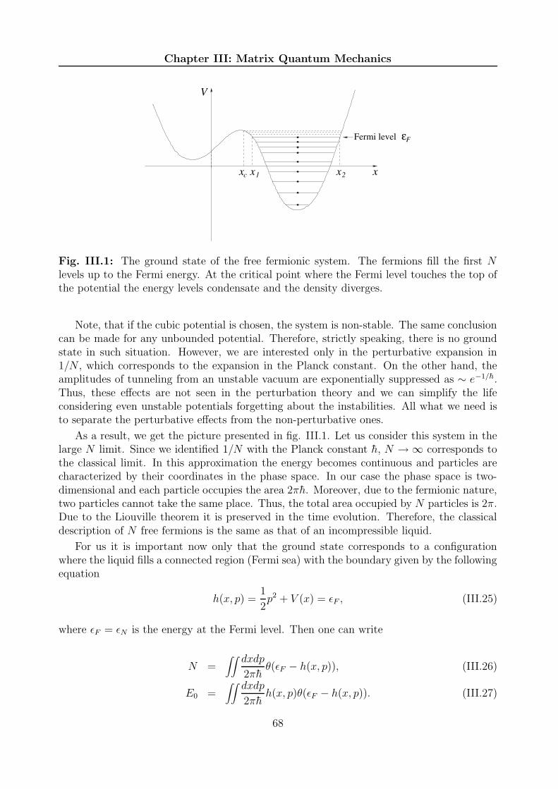
Chapter III: Matrix Quantum Mechanics
x2
V
xx1
Fermi level
xc
Fε
Fig. III.1: The ground state of the free fermionic system. The fermions fill the first Nlevels up to the Fermi energy. At the critical point where the Fermi level touches the top ofthe potential the energy levels condensate and the density diverges.
Note, that if the cubic potential is chosen, the system is non-stable. The same conclusioncan be made for any unbounded potential. Therefore, strictly speaking, there is no groundstate in such situation. However, we are interested only in the perturbative expansion in1/N , which corresponds to the expansion in the Planck constant. On the other hand, theamplitudes of tunneling from an unstable vacuum are exponentially suppressed as ∼ e−1/h.Thus, these effects are not seen in the perturbation theory and we can simplify the lifeconsidering even unstable potentials forgetting about the instabilities. All what we need isto separate the perturbative effects from the non-perturbative ones.
As a result, we get the picture presented in fig. III.1. Let us consider this system in thelarge N limit. Since we identified 1/N with the Planck constant h, N → ∞ corresponds tothe classical limit. In this approximation the energy becomes continuous and particles arecharacterized by their coordinates in the phase space. In our case the phase space is two-dimensional and each particle occupies the area 2πh. Moreover, due to the fermionic nature,two particles cannot take the same place. Thus, the total area occupied by N particles is 2π.Due to the Liouville theorem it is preserved in the time evolution. Therefore, the classicaldescription of N free fermions is the same as that of an incompressible liquid.
For us it is important now only that the ground state corresponds to a configurationwhere the liquid fills a connected region (Fermi sea) with the boundary given by the followingequation
h(x, p) =1
2p2 + V (x) = εF , (III.25)
where εF = εN is the energy at the Fermi level. Then one can write
N =∫∫
dxdp
2πhθ(εF − h(x, p)), (III.26)
E0 =∫∫
dxdp
2πhh(x, p)θ(εF − h(x, p)). (III.27)
68

§2 Singlet sector and free fermions
Differentiation with respect to εF gives
h∂N
∂εF
def= ρ(εF ) =
∫∫
dxdp
2πδ(εF − h(x, p)) =
1
π
x2∫
x1
dx√
2(εF − V (x)), (III.28)
h∂E0
∂εF=
∫∫
dxdp
2πh(x, p)δ(εF − h(x, p)) = εFρ(εF ), (III.29)
where x1 and x2 are turning points of the classical trajectory at the Fermi level. Theseequations determine the energy in an inexplicit way.
To find the energy in terms of the coupling constants, one should exclude the Fermilevel εF by means of the normalization condition (III.26). For some simple potentials theintegral in (III.26) can be calculated explicitly, but in general this cannot be done. However,the universal information related to the sum over continuous surfaces and 2D string theoryis contained only in the singular part of the free energy. The singularity appears whenthe Fermi level reaches the top of the potential similarly to the one-matrix case (cf. figs.III.1 and II.4). Near this point the density diverges and shows together with the energy anon-analytical behaviour.
From this it is clear that the singular contribution to the integral (III.28) comes fromthe region of integration around the maxima of the potential. Generically, the maxima areof the quadratic type. Thus, up to analytical terms we have
x2∫
x1
dx√
2(εF − V (x))∼ −1
2log(εc − εF ), (III.30)
where εc is the critical value of the Fermi level. Denoting ε = εc − εF , one finds [43]
ρ(ε) = − 1
2πlog(ε/Λ), F0 =
1
4πh2 ε2 log(ε/Λ), (III.31)
where we introduced a cut-off Λ related to the non-universal contributions.
2.4 Double scaling limit
In the previous paragraph we reproduced the free energy and the density of states in theplanar limit. To find them in all orders in the genus expansion, one needs to consider thedouble scaling limit as it was explained in section II.2.5. For this one should correlate thelarge N limit with the limit where the coupling constants approach their critical values. Inour case this means that one should introduce coordinates describing the region near the topof the potential. Let xc is the coordinate of the maximum and y = 1√
h(x − xc). Then the
potential takes the form
V (y) = εc −h
2y2 +
h3/2λ
3y3 + · · · , (III.32)
where the dots denote the terms of higher orders in h. The Schrodinger equation for theeigenfunction at the Fermi level can be rewritten as follows
(
−1
2
∂2
∂y2− 1
2y2 +
h1/2λ
3y3 + · · ·
)
ψN (y) = −h−1εψN (y). (III.33)
69

Chapter III: Matrix Quantum Mechanics
It shows that it is natural to define the rescaled energy variable
µ = h−1(εc − εF ). (III.34)
This relation defines the double scaling limit of MQM, which is obtained as N = h−1 → ∞,εF → εc and keeping µ to be fixed [75, 76, 77, 78].
Note that the double scaling limit (III.34) differs from the naive limit expected from1MM where we kept fixed the product of N and some power of λc − λ (II.21). In ourcase the latter is renormalized in a non-trivial way. To get this renormalization, note thatwriting the relation (III.28) we actually decoupled N and h. This means that in fact werescaled the argument of the potential so that we moved the coupling constant from thepotential to the coefficient in front of the action. For example, we can do this with thecubic coupling constant λ by rescaling x→ x/λ. In this normalization the overall coefficientshould be multiplied by λ−2 what changes the relation between N and the Planck constantto h = λ2/N . Then for ∆ = 2π
h(λ2
c − λ2), (III.28) and (III.34) imply
∂∆
∂µ= 2πρ(µ). (III.35)
Integrating this equation, one finds a complicated relation between two scaling variables. Inthe planar limit this relation reads
∆ = −µ log(µ/Λ). (III.36)
The remarkable property of the double scaling limit (III.34) is that it reduces the problemto the investigation of free fermions in the inverse oscillator potential Vds(x) = −1
2x2
−1
2
(
∂2
∂x2+ x2
)
ψε(x) = εψε(x), (III.37)
where we returned to the notations x and ε for already rescaled matrix eigenvalues and energy.All details of the initial potential disappear in this limit because after the rescaling the cubicand higher terms suppressed by positive powers of h. This fact is the manifestation of theuniversality of MQM showing the independence of its results of the form of the potential.
The equation (III.37) for eigenfunctions has an explicit solution in terms of the paraboliccylinder functions. They have a complicated form and we do not give their explicit expres-sions. However, the density of states at the Fermi level can be calculated knowing only theirasymptotics at large x. The density follows from the WKB quantization condition
(
Φεn+1 − Φεn
)∣
∣
∣√Λ
= 2π, (III.38)
where Φε is the phase of the wave function ψε(x) = C√xeiΦε(x) and the difference is calculated
at the cut-off x ∼√
Λ ∼√N . The asymptotic form of the phase is [79]
Φε(x) ≈ 1
2x2 + ε log x− φ(ε), (III.39)
φ(ε) =π
4− i
2log
Γ(12
+ iε)
Γ(12− iε)
. (III.40)
70
§2 Singlet sector and free fermions
In the WKB approximation the index n becomes continuous variable and the density ofstates is defined as its derivative
ρ(ε)def=∂n
∂ε=
1
2πlog Λ − 1
2π
dφ
dε=
1
2πlog Λ − 1
2πReψ(
1
2+ iε), (III.41)
where ψ(ε) = ddε
log Γ(ε). Neglecting the cut-off dependent term and expanding the digammafunction in 1/µ (µ = −ε), one finds the following result
ρ(µ) =1
2π
(
− logµ+∞∑
n=1
(22n−1 − 1)|B2n|n
(2µ)−2n
)
, (III.42)
where B2n are Bernoulli numbers. Integrating (III.29), one obtains the expansion of the freeenergy
F (µ) =1
4π
(
µ2 logµ− 1
12logµ+
∞∑
n=1
(22n+1 − 1)|B2n+2|4n(n + 1)
(2µ)−2n
)
. (III.43)
In fact, to compare this result with the genus expansion of the partition function of 2Dstring theory, one should reexpand (III.43) in terms of the renormalized string coupling. Itsrole, as usual, is played by κ = ∆−1 and its relation to µ is determined by (III.35). With ρ(µ)taken from (III.42), one can solve this equation with respect to ∆(µ). Then it is sufficientto make substitution into (III.43) to get the following answer
F (∆) =1
4π
∆2
log ∆− 1
12log ∆ +
∞∑
n=1
(22n+1 − 1)|B2n+2|4n(n+ 1)(2n+ 1)
(
2∆
log ∆
)−2n
, (III.44)
where terms O(log−1 ∆) were neglected because they contain the cut-off and vanish in thedouble scaling limit.
Some remarks related to the expansion (III.44) are in order. First, the coefficients asso-ciated with genus g grow as (2g)!. This behaviour is characteristic for closed string theorieswhere the sum over genus-g surfaces exhibits the same growth. Besides, we observe a newfeature in comparison with the one-matrix model. Although the couplings were renormal-ized, the sums over spherical and toroidal surfaces logarithmically diverge. This also can beexplained in the context of the CFT approach. Finally, comparing (III.44) with (II.19), wefind that the string susceptibility for MQM vanishes γstr = 0. This is again in the excellentagreement with the continuum prediction of [80].
Thus, all results concerning the free energy of MQM coincide with the correspondingresults for the partition function of 2D string theory. Therefore, it is tempting to claimthat they are indeed equivalent theories. But we know that 2D string theory possessesdynamical degrees of freedom: the tachyon, winding modes and discrete states. To justifythe equivalence further, we should show how all of them are realized in Matrix QuantumMechanics.
71

Chapter III: Matrix Quantum Mechanics
3 Das–Jevicki collective field theory
The fermionic representation presented in the previous section gives a microscopic descriptionof 2D string theory. As usual, the macroscopic description, which has a direct interpretationin terms of the target space fields of 2D string theory, is obtained as a theory of effectivedegrees of freedom. These degrees of freedom are collective excitations of the fermions ofthe singlet sector of MQM and identified with the tachyonic modes of 2D strings. Theirdynamics is governed by a collective field theory [81], which in the given case was developedby Das and Jevicki [82]. This theory encodes all interactions of strings in two dimensionsand, therefore, it gives an example of string field theory formulated directly in the targetspace.
3.1 Effective action for the collective field
A natural collective field in MQM is the density of eigenvalues
ϕ(x, t) = tr δ (x−M(t)) . (III.45)
In the double scaling limit, which implies N → ∞, it becomes a continuous field. Itsdynamics can be derived directly from the MQM action with the inverse oscillator potential[82]
S =1
2
∫
dt tr(
M2 +M2)
. (III.46)
However, it is much easier to use the Hamiltonian formulation. The Hamiltonian of MQM inthe singlet representation is given by the energy of the Fermi sea similarly to the ground stateenergy (III.27). The difference is that now the Fermi sea can have an arbitrary profile whichcan differ from the trajectory of one fermion (III.25). Besides, to the expression (III.27) oneshould add a term which fixes the Fermi level and allows to vary the number of fermions.Otherwise the density would be subject of some normalization condition. Thus, the fulldouble scaled Hamiltonian reads
Hcoll =∫∫
Fermisea
dxdp
2π(h(x, p) + µ), (III.47)
where
h(x, p) =1
2p2 + V (x), V (x) = −1
2x2. (III.48)
We restrict ourselves to the case where the boundary of the Fermi sea can be representedby two functions, say p+(x, t) and p−(x, t) satisfying the boundary condition p+(x∗, t) =p−(x∗, t), where x∗ is the leftmost point of the sea (fig. III.2a). It means that we forbid thesituations shown on fig, III.2b. In the fermionic picture they do not cause any problems, butin the bosonic description they require a special attention.
In this restricted situation one can take the integral over the momentum in (III.47). Theresult is
Hcoll =∫ dx
2π
(
1
6(p3
+ − p3−) + (V (x) + µ)(p+ − p−)
)
. (III.49)
72

§3 Das–Jevicki collective field theory
p
x
a)
p+
−p
*x
p
x
b)
Fig. III.2: The Fermi sea of the singlet sector of MQM. The first picture shows the situationwhere the profile of the Fermi sea can be described by a two-valued function. The secondpicture presents a more general configuration.
It is clear that the difference of p+ and p− coincides with the density (III.45), whereas theirsum plays the role of a conjugate variable. The right identification is the following [83]:
p±(x, t) = ∂xΠ ± πϕ(x, t), (III.50)
where the equal-time Poisson brackets are defined as
ϕ(x),Π(y) = δ(x− y). (III.51)
Substitution of (III.50) into (III.49) gives
Hcoll =∫
dx
(
1
2ϕ(∂xΠ)2 +
π2
6ϕ3 + (V (x) + µ)ϕ
)
. (III.52)
One can exclude the momentum Π(x, t) by means of the equation of motion
−∂xΠ =1
ϕ
∫
dx∂tϕ (III.53)
what leads to the following collective field theory action
Scoll =∫
dt∫
dx
(
1
2ϕ
(∫
dx∂tϕ)2
− π2
6ϕ3 − (V (x) + µ)ϕ
)
. (III.54)
This action can be considered as a background independent formulation of string fieldtheory. It contains a cubic interaction and a linear tadpole term. The former describes theeffect of splitting and joining strings and the latter represents a process of string annihilationinto the vacuum. The important point is that the dynamical field ϕ(x, t) is two-dimensional.The dimension additional to the time t appeared from the matrix eigenvalues. This showsthat the target space of the corresponding string theory is also two-dimensional in agreementwith our previous conclusion.
73

Chapter III: Matrix Quantum Mechanics
Another observation is that whereas the initial matrix model in the inverse oscillatorpotential was simple with the linear equations of motion
..
M(t) −M(t) = 0, (III.55)
the resulting collective field theory is non-linear. Thus, MQM provides a solution of acomplicated non-linear theory through the transformation of variables (III.45). Nevertheless,the integrability of MQM is present also in the effective theory (III.54). Indeed, consider theequations of motion for the fields p+ and p−. The equations (III.50) and (III.51) imply thefollowing Poisson brackets
p±(x), p±(y) = ∓2π∂xδ(x− y) (III.56)
so that the Hamiltonian (III.49) gives
∂tp± + p±∂xp± + ∂xV (x) = 0. (III.57)
This equation is a KdV type equation which is integrable. This indicates that the wholetheory is also exactly solvable. In fact, one can write an infinite set of conserved commutingquantities [83]
Hn =∫∫
Fermisea
dxdp
2π(p2 − x2)n. (III.58)
It is easy to check that up to surface terms they satisfy
Hn, Hm = 0 andd
dtHn = 0. (III.59)
The quantities Hn can be considered as Hamiltonians generating some perturbations. Sinceall of them are commuting, according to the definition given in section II.5.1, we concludethat the system is integrable.
3.2 Identification with the linear dilaton background
Now we choose a particular background of string theory. This will allow to identify thetachyon field and target space coordinates with the corresponding quantities of the collectivefield theory. In terms of the collective theory the choice of a background means to considerthe perturbation theory around some classical solution of (III.54). We choose the solutiondescribing the ground state of MQM. It is obtained from (III.25) and can be written as
πϕ0 = ±p± =√
x2 − 2µ. (III.60)
This solution is distinguished by the fact that it is static and that the boundary of the Fermisea coincides with a trajectory of one fermion.
Taking (III.60) as a background, we are interested in small fluctuations of the collectivefield around this background solution
ϕ(x, t) = ϕ0(x) +1√π∂xη(x, t). (III.61)
74
§3 Das–Jevicki collective field theory
The dynamics of these fluctuations is described by the following action obtained by substi-tution of (III.61) into (III.54)
Scoll =1
2
∫
dt∫
dx
(
(∂tη)2
(πϕ0 +√π∂xη)
− πϕ0(∂xη)2 −
√π
3(∂xη)
3
)
. (III.62)
The expansion of the denominator in the first term gives rise to an infinite number ofvertices of increasing order with the field η. A compact version of this interacting theorywould be obtained if we worked with the Hamiltonian instead of the action. Then only cubicinteraction terms would appear.
Let us consider the quadratic part of the action (III.62). It is given by
S(2) =1
2
∫
dt∫
dx
(
(∂tη)2
πϕ0− (πϕ0)(∂xη)
2
)
. (III.63)
Thus, η(x, t) can be interpreted as a massless field propagating in the background metric
g(0)µν =
(−πϕ0 00 (πϕ0)
−1
)
. (III.64)
However, the non-trivial metric can be removed by a coordinate transformation. It is enoughto introduce the time-of-flight coordinate
q(x) =
x∫
dx
πϕ0(x). (III.65)
The change of coordinate (III.65) brings the action to the form
Scoll =1
2
∫
dt∫
dq
(
(∂tη)2 − (∂qη)
2 − 1
3π√πϕ2
0
(
(∂qη)3 + 3(∂qη)(∂tη)
2)
+ · · ·)
, (III.66)
where we omitted the terms of higher orders in η. The action (III.66) describes a masslessfield in the flat Minkowski spacetime with a spatially dependent coupling constant
gstr(q) =1
(πϕ0(q))2. (III.67)
Using the explicit formula (III.60) for the background solution, one can obtain
x(q) =√
2µ cosh q, p(q) =√
2µ sinh q. (III.68)
Thus, the coupling constant behaves as
gstr(q) =1
2µ sinh2 q∼ 1
µe−2q, (III.69)
where the asymptotics is given for q → ∞.Comparing (III.69) with (I.25), we see that the collective field theory action (III.66)
describes 2D string theory in the linear dilaton background. In the asymptotic region of
75

Chapter III: Matrix Quantum Mechanics
large q the flat coordinates (t, q) can be identified with the coordinates of the target space ofstring theory coming from the c = 1 matter X and the Liouville field φ on the world sheet.The identification reads as follows
it ↔ X, q ↔ φ. (III.70)
Thus, the time of MQM and the time-of-flight coordinate, which is a function of the matrixeigenvalue variable, form the flat target space of the linear dilaton background. It is alsoclear that the two-dimensional massless collective field η(q, t) coincides with the redefinedtachyon η = e2φT .
In fact, the above identification is valid only asymptotically. When we go to the regionof small q, one should include into account the Liouville exponent µe−2φ in the CFT action(I.39). The tachyon field can be considered as a wave function describing the lowest eigenstateof the Hamiltonian of this CFT. Therefore, instead of Klein–Gordon equation, it shouldsatisfy the Liouville equation
(
∂2X + ∂2
φ + 4∂φ + 4 − µe−2φ)
T (φ,X) = 0. (III.71)
Hence the Liouville mode does not coincide exactly with the collective field coordinate q. Thecorrect identification is obtained as follows [84]. We return to the eigenvalue variable x andconsider its conjugated momentum p = −i∂/∂x. The Fourier transform of the Klein–Gordonequation written in the metric (III.64) gives(
∂2t −
√
x2 − 2µ∂x√
x2 − 2µ∂x
)
η(x, t) = 0 ⇒(
∂2t − (p∂p)
2 − 2p∂p − 1 − 2µp2)
η(p, t) = 0.
(III.72)where η is the Fourier image of η. Finally, the change of variables
it = X, ip =1√2e−φ (III.73)
together with T (φ,X) ∼ p3η(p, t) brings (III.72) to the Liouville equation (III.71). Thisshows that, more precisely, the Liouville coordinate is identified with the logarithm of themomentum conjugated to the matrix eigenvalue.
The meaning of this rule becomes more clear after realizing that the Fourier transformwith an imaginary momentum of the collective field ϕ is the Wilson loop operator
W (l, t) = tr(
e−lM)
=∫
dxe−lxϕ(x, t). (III.74)
This operator inserts a loop of the length l into the world sheet. Therefore, it has a directgeometrical interpretation and its parameter l is related to the scale of the metric, whichis governed by the Liouville mode φ. Thus, it is quite natural that l and φ are identifiedthrough (III.73) where one should take ip = l. The substitution of the expansion (III.61)gives
W (l, t) = W0 +1√π
∫
dxe−lx∂xη(x, t) = W0 +l√πη(−il, t), (III.75)
where
W0 =
√2µ
lK1(
√
2µl) (III.76)
76

§3 Das–Jevicki collective field theory
is the genus zero one-point function of the density. Using this representation, it is easy tocheck that the Wilson loop operator satisfies the following Wheeler–DeWitt equation [85]
(
∂2t − (l∂l)
2 + 2µl2)
W (l, t) = 0. (III.77)
Thus, in the l-representation it is the Wilson loop operator that is the analog of the freefield for which the derivative terms have standard form. Therefore, we should identify thefield η from section I.5.1 with W rather than with η defined in (III.72). The precise relationbetween the tachyon field and the Wilson loop operator is the following
T (φ,X) = e−2φW (l(φ),−iX) = e−2φW0 + e−2φ
∞∫
0
dq exp[
−√µe−φ cosh q
]
∂qη. (III.78)
The integral transformation (III.78) expresses solutions of the non-linear Liouville equa-tion through solutions of the Klein–Gordon equation, This reduces the problem of calculatingthe tachyon scattering amplitudes in the linear dilaton background to calculation of the S-matrix for the collective field theory of the Klein–Gordon field η. As we saw above, thistheory is integrable. Therefore, the scattering problem in 2D string theory can be exactlysolved. Before to show that, we should introduce the operators creating the asymptoticstates, i.e., the tachyon vertex operators.
3.3 Vertex operators and correlation functions
The vertex operators of the tachyon field were constructed in section I.5.1. Their Minkowskianform is given by (I.44) and describes the left and right movers. Note that the representationfor the operators was written only in the asymptotic region φ → ∞ where the Liouvillepotential can be ignored. Therefore, we can use the simple identification (III.70) to relatethe matrix model quantities with the target space objects. Then one should find operatorsthat behave as left and right movers in the space of t and q.
First, the t-dependence of a matrix model operator is completely determined by theinverse oscillator potential, which leads to the following simple Heisenberg equation
∂
∂tA(t) = i
[
1
2(p2 − x2), A(t)
]
. (III.79)
Its solution is conveniently represented in the basis of the chiral operators
x±(t)def=x(t) ± p(t)√
2= x±(0)e±t. (III.80)
Therefore, the time-independent operators, which should be used in the Schrodinger repre-sentation, are e∓tx±(t). This suggests that the vertex operators can be constructed frompowers of x±. Indeed, it was argued [83] that their matrix model realization is given by
T±n = e±nt tr (M ∓ P )n. (III.81)
77

Chapter III: Matrix Quantum Mechanics
To justify further this choice, let us consider the collective field representation of theoperators (III.81)
T±n = e±nt
∫
dx
2π
p+(x,t)∫
p−(x,t)
dp (x∓ p)n =e±nt
n+ 1
∫
dx
2π(x∓ p)n+1
∣
∣
∣
∣
∣
p+
p−
, (III.82)
where p± are second quantized fields satisfying equations (III.57). We shift these fields bythe classical solution
p±(x, t) = ±πϕ0(x) +α∓(x, t)
πϕ0(x). (III.83)
Then the linearized equations of motion for the quantum corrections α± coincide with theconditions for chiral fields
(∂t ∓ ∂q)α± = 0 ⇒ α± = α±(t± q). (III.84)
In the asymptotics q → ∞, πϕ0 ≈ x ≈ 12eq. Therefore, in the leading approximation the
operators (III.82) read
T±n ≈
∫ dq
2πen(q±t)α±. (III.85)
The integral extracts the operator creating the component of the chiral field which behavesas en(q±t). This shows that the matrix operators (III.81) do possess the necessary properties.The factor e−2φ, which is present in the definition of the vertex operators (I.44) and absentin the matrix case, can be seen as coming from the measure of integration over the worldsheet or, equivalently, as a result of the redefinition of the tachyon field (III.78). In fact, itis automatically restored by the matrix model.
The matrix operators (III.81) correspond to the Minkowskian vertex operators with imag-inary momenta k = in. After the continuation of time to the Euclidean region t → −iX,they also can be considered as vertex operators with Euclidean momenta p = ∓n. To realizeother momenta, one should analytically continue from this discrete set to the whole complexplane. In particular, the vertex operators of Minkowskian real momenta are obtained as
V ±k ∼ T±
−ik = e∓ikt tr (M ∓ P )−ik. (III.86)
Using these operators, one can construct and calculate scattering amplitudes of tachyons.The result has been obtained from both the collective field theory formalism [86, 87, 88, 89]and the fermionic representation [26, 90, 91, 92, 79]. Moreover, the generating functionalfor all S-matrix elements has been constructed [92]. It takes an especially transparent formwhen the S-matrix is represented as a composition of three processes: fermionization ofincoming tachyon modes, scattering in the free fermion theory and reverse bosonization ofthe scattered fermions
STT = ιf→b SFF ιb→f . (III.87)
The fermionic S-matrix SFF was explicitly calculated from the properties of the paraboliccylinder functions [91]. We do not give more details since these results will be reproducedin much simpler way from the formalism which we develop in the next chapters.
78

§3 Das–Jevicki collective field theory
We restrict ourselves to two remarks. The first one is that in those cases where thescattering amplitudes in 2D string theory can be calculated by the CFT methods, the resultscoincided with the corresponding calculations in MQM [93]. The only thing to be done toensure the complete agreement is a local redefinition of the vertex operators. It turns out thatthe exact relation between the tachyon operators (I.44) and their matrix model realization(III.81) include the so called leg-factors [94]
V +k =
Γ(−ik)Γ(ik)
T+−ik, V −
k =Γ(ik)
Γ(−ik)T−−ik. (III.88)
This redefinition is not surprising because the matrix model gives only a discrete approxima-tion to the local vertex operators and in the continuum limit the operators can be renormal-ized. Therefore, one should expect the appearance of such leg-factors in any matrix/stringcorrespondence. Note that the Minkowskian leg-factors (III.88) are pure phases. Thus, theyrepresent a unitary transformation and do not affect the amplitudes. However, they arerelevant for the correct spacetime physics, in particular, for the gravitational scattering oftachyons [89]. In fact, the leg-factors can be associated with a field redefinition given bythe integral transformation (III.78). Written in the momentum space for q, it gives rise toadditional factors for the left and right components whose ratio produces the leg-factor.
The second remark is that in the case when the Euclidean momenta of the incomingand outgoing tachyons belong to an equally spaced lattice (as in a compactified theory), thegenerating functional for S-matrix elements has been shown to coincide with a τ -functionof Toda hierarchy [92]. However, this fact has not been used to address other problems likescattering in presence of a tachyon condensate. We will show that with some additionalinformation added, it allows to solve many interesting questions related to 2D string theoryin non-trivial backgrounds.
3.4 Discrete states and chiral ring
Finally, we show how the discrete states of 2D string theory appear in MQM. They arecreated by a natural generalization of the matrix operators (III.81) [95]
Tn,n = e(n−n)t tr ((M + P )n(M − P )n) (III.89)
which have the following Euclidean momenta
pX = i(n− n), pφ = n + n− 2. (III.90)
Comparing with the momenta of the discrete states (I.49), one concludes that
m =n− n
2, j =
n+ n
2. (III.91)
Taking into account that n and n are integers, one finds that the so defined pair (j,m) spansall discrete states.
It is remarkable that the collective field theory approach allows to unveil the presence ofa large symmetry group [95, 84, 25]. Indeed, the operators (III.89) are realized as
Tj,m = e−2mt∫
dx
2π
p+∫
p−
dp (x+ p)j+m(x− p)j−m, (III.92)
79

Chapter III: Matrix Quantum Mechanics
where we changed indices of the operator from n, n to j,m. One can check that they obeythe commutation relations of w∞ algebra
Tj1,m1 , Tj2,m2 = 4i (j1m2 − j2m1)Tj1+j2−1,m1+m2 . (III.93)
In particular, the operators Tj,m are eigenstates of the Hamiltonian H = − 12T1,0
H, Tj,m = −2imTj,m (III.94)
what means that they generate its spectrum. When we replace the Poisson brackets of theclassical collective field theory by the quantum commutators, the w∞ algebra is promotedto a W1+∞ algebra.
Each generator (III.89) gives rise to an element of the ground ring of the c = 1 CFT [25]which plays an important role in many physical problems. First, we introduce the so calledchiral ground ring. It consists of chiral ghost number zero, conformal spin zero operatorsOJM which are closed under the operator product O · O′ ∼ O′′ up to BRST commutators.The entire chiral ring can be generated from the basic operators
O0,0 = 1,
ydef= O 1
2, 12
= (cb + i∂X − ∂φ) eiX+φ, (III.95)
wdef= O 1
2,− 1
2= (cb− i∂X − ∂φ) e−iX+φ.
The ground ring is constructed from products of the chiral and antichiral operators. Weconsider the case of the theory compactified at the self-dual radius R = 1 in the absence ofthe cosmological constant µ. Then the ground ring contains the following operators
Vj,m,m = Oj,mOj,m. (III.96)
The ring has four generators
a1 = yy, a2 = ww, a3 = yw, a4 = wy. (III.97)
These generators obey one obvious relation which determines the ground ring of the c = 1theory
a1a2 − a3a4 = 0. (III.98)
It has been shown [25] that the symmetry algebra mentioned above is realized on thisground ring as the algebra of diffeomorphisms of the three dimensional cone (III.98) pre-serving the volume form
Θ =da1da2da3
a3. (III.99)
Furthermore, it was argued that the inclusion of perturbations by marginal operators deformsthe ground ring to
a1a2 − a3a4 = M(a1, a2), (III.100)
where M is an arbitrary function. In particular, to introduce the cosmological constant, oneshould take M to be constant. As a result, one removes the conic singularity and obtains asmooth manifold
a1a2 − a3a4 = µ. (III.101)
80
§3 Das–Jevicki collective field theory
In the limit of uncompactified theory only the generators a1 and a2 survive. The symme-try of volume preserving diffeomorphisms is reduced to some abelian transformations plusarea preserving diffeomorphisms of the plane (a1, a2) that leave fixed the curve
a1a2 = µ (III.102)
or its deformation according to (III.100). The suggestion was to identify the plane (a1, a2)with the eigenvalue phase space of MQM. Namely, one has the following relations
a1 = x + p, a2 = x− p. (III.103)
Then it is clear that equation (III.102) corresponds to the Fermi surface of MQM. Thementioned abelian transformations are associated with time translations. And the operators(III.89) are identified with an1a
n2 .
The sense of the operators a3 and a4 existing in the compactified theory is also known.They correspond to the winding modes of strings which we are going to consider in the nextsection. The relation (III.101) satisfied by these operators is very important because it showshow to describe the theory containing both the tachyon and winding modes. However, ithas not been yet understood how to obtain this relation directly from MQM.
81
Chapter III: Matrix Quantum Mechanics
4 Compact target space and winding modes in MQM
In the previous section we showed that the modes of 2D string theory in the linear dila-ton background are described by the collective excitations of the singlet sector of MatrixQuantum Mechanics. If we compactify the target space of string theory, then there appearadditional states — windings of strings around the compactified dimension. In this sectionwe demonstrate how to describe these modes in the matrix language.
4.1 Circle embedding and duality
In matrix models the role of the target space of non-critical string theory is played by theparameter space of matrices. Therefore, to describe 2D string theory with one compactifieddimension one should consider MQM on a circle. The partition function of such matrixmodel is given by the integral (III.1) where the integration is over a finite Euclidean timeinterval t ∈ [0, β] with the two ends identified. The length of the interval is β = 2πR whereR is the radius of the circle. The identification t ∼ t + β requires to impose the periodicboundary condition M(0) = M(β). Thus, one gets
ZN(R, g) =∫
M(0)=M(β)
DM(t) exp
−N tr
β∫
0
dt(
1
2M2 + V (M)
)
. (III.104)
As usual, one can write the Feynman expansion of this integral. It is the same as in(III.3) with the only difference that the propagator should be replaced by the periodic one
G(t) =∞∑
m=−∞e−|t+mβ|. (III.105)
We see that for large β the term m = 0 dominates and we return to the uncompactified case.But for finite β the sum should be retained and this leads to important phenomena relatedwith the appearance of vortices on the discretized world sheet [96, 97, 98, 99].
We mentioned in section I.5.3 that the c = 1 string theory compactified at radius R is T-dual to the same theory at radius 1/R. Does this duality appear in the sum over discretizedsurfaces regularizing the sum over continuous geometries? To answer this question, weperform the duality transformation of the Feynman expansion of the matrix integral (III.104)
F =∞∑
g=0
N2−2g∑
connecteddiagrams Γg
λVV∏
i=1
β∫
0
dti∏
〈ij〉
∞∑
mij=−∞e−|ti−tj+βmij |, (III.106)
where we have chosen for simplicity the cubic potential (II.15). The duality transformationis obtained applying the Poisson formula to the propagator (III.105)
G(ti − tj) =1
β
∞∑
kij=−∞ei
2πβkij(ti−tj)G(kij) =
1
β
∞∑
kij=−∞ei
2πβkij(ti−tj) 2
1 +(
2πβkij)2 . (III.107)
82
§4 Compact target space and winding modes in MQM
The substitution of (III.107) into (III.106) allows to integrate over ti which gives the mo-mentum conservation constraint at each vertex
kij1 + kij2 + kij3 = 0. (III.108)
This reduces the number of independent variables from E to E − V + 1. (One additionaldegree of freedom appears due to the zero mode which is canceled in all ti− tj .) By virtue ofthe Euler theorem this equals to L−1+2g. According to this, we attach a momentum pI toeach elementary loop (face) of the graph (one of pI is fixed) and define remaining 2g variablesas momenta la running along independent non-contractable loops. Thus, one arrives at thefollowing representation
F =∞∑
g=0
(
Nβ
λ2
)2−2g∑
connecteddiagrams Γ
(
λ2
β
)L
L−1∏
I=1
∞∑
pI=−∞
2g∏
a=1
∞∑
la=−∞
∏
〈IJ〉G
pI − pJ +2g∑
a=1
laεaIJ
,
(III.109)where the sum goes over the dual graphs (triangulations) with L dual vertices and weintroduced the matrix εaIJ equal ±1 when a dual edge 〈IJ〉 crosses an edge belonging to athnon-contractable cycle (the sign depends on the mutual orientation) and zero otherwise.
The transformation (III.107) changes R → 1/R which is seen from the form of thepropagators. But the result (III.109) does not seem to be dual to the original representation(III.106). Actually, at the spherical level, instead of describing a compact target space ofthe inverse radius, it corresponds to the embedding into the discretized real line with latticespacing 1/R [26]. This is natural because the variables pI live in the momentum space ofthe initial theory which is discrete.
Thus, even in the continuum limit, the sum over discretized surfaces embedded in acircle cannot be identical to its continuum analog. The reason is that it possesses additionaldegrees of freedom which are ignored in the naive continuum limit. These are the vortexconfigurations. Indeed, in the continuum geometry the simplest vortex of winding numbern is described by the field X(θ) = nRθ where θ is the azimuth angle. However, this is asingular configuration and should be disregarded. In contrast, on a lattice the singularityis absent and such configurations are included into the statistical sum. For example, in thenotations of (III.106) the number of vortices associated with a face I is given by
wI =∑
〈ij〉∈Imij. (III.110)
It is clear that it coincides with the number of times the string is wrapped around the circle.In other words, the vortices are world sheet realizations of windings in the target space. Thus,MQM with compactified time intrinsically contains winding string configurations. But justdue to this fact, it fails to reproduce the partition function of compactified 2D string theory.
It is clear that to obtain the sum over continuous surfaces possessing selfduality oneshould somehow exclude the vortices. This can be done restricting the sum over mij in(III.106). The distribution mij can be seen as an abelian gauge field defined on links of agraph. Then the quantity (III.110) is its field strength. We want that this strength vanishes.With this condition only the ”pure gauge” configurations of mij are admissible. They are
83

Chapter III: Matrix Quantum Mechanics
represented as
mij = mi −mj +2g∑
a=1
εaij la, (III.111)
where integers la are associated with non-contractable loops of the dual graph and εaij is thematrix dual to εaIJ . If we change the sum over all mij by the sum over these pure gaugeconfigurations, the free energy (III.106) is rewritten as follows
F = β∞∑
g=0
N2−2g∑
connecteddiagrams Γg
λVV−1∏
i=1
∞∫
−∞dti
2g∏
a=1
∞∑
la=−∞
∏
〈ij〉exp
−|ti − tj + β2g∑
a=1
εaij la|
, (III.112)
where the overall factor β arises from the integration over the zero mode. The sum overmi resulted in the extension of the integrals over ti to the whole line. Due to this the dualtransformation gives rise to integrals over momenta rather than discrete sums. Repeatingthe steps which led to (III.109) and renormalizing the momenta, one obtains
F = 2πR
∞∑
g=0
(
Nβλ2
)2−2g∑
connecteddiagrams Γ
(
λ2
4π2
)L(
L−1∏
I=1
∞∫
−∞dpI
)
×
×(
2g∏
a=1
∞∑
la=−∞
)
∏
〈IJ〉2
1+ 14π2
(
pI−pJ+ 2πR
2g∑
a=1
laεaIJ
)2 . (III.113)
The only essential difference between two representation (III.112) and (III.113) is thepropagator. However, the universality of the continuum limit implies that the results in themacroscopic scale do not depend on it. Moreover, if we choose the Gaussian propagator,which follows from the usual Polyakov action, its Fourier transform coincides with the originalone. Due to this one can neglect this discrepancy. Then the two representations are dual toeach other with the following matching of the arguments
R → 1/R, N → RN. (III.114)
Thus, the exclusion of vortices allowed to make the sum over discretized surfaces selfdualand they are those degrees of freedom that are responsible for the breaking of this dualityin the full matrix integral.
We succeeded to identify and eliminate the vortices in the sum over discretized surfaces.How can this be done directly in the compactified Matrix Quantum Mechanics defined bythe integral (III.104)? In other words, what matrix degrees of freedom describe the vortices?Let us see how MQM in the Hamiltonian formulation changes after compactification. Thepartition function is represented by the trace in the Hilbert space of the theory of theevolution operator as in (III.16)
ZN(R) = Tr e−βhH
MQM . (III.115)
Now the time interval coincides with β which can also be considered as the inverse temper-ature. It is finite so that one should consider the finite temperature partition function. This
84
§4 Compact target space and winding modes in MQM
fact drastically complicates the problem because one should take into account the contribu-tions of all states and not only the ground state. In particular, all representations of theSU(N) global symmetry group come to the game. The states associated with these represen-tations are those additional states which appear in the compactified theory. Therefore, it isnatural to expect that they correspond to vortices on the discretized world sheet or windingsof the string [99, 100].
The first check of this expectation which can be done is to verify the duality (III.114).Since we expect vortices only in the non-singlet representations of SU(N), to exclude themone should restrict oneself to the singlet sector as in the uncompactified theory. Then westill have a powerful description in terms of free fermions. In the double scaling limit, we areinterested in, the fermions move in the inverse oscillator potential. Thus we return to theproblem stated by equation (III.37). However, the presence of a finite temperature gives riseto a big difference with the previous situation. Due to the thermal fluctuations, the Fermisurface cannot be defined in the ensemble with fixed number of particles N . The solution isto pass to the grand canonical ensemble with the following partition function
Z(µ,R) =∞∑
N=0
e−βµNZN(R). (III.116)
The chemical potential µ is exactly the Fermi level which is considered now as the basicvariable while N becomes an operator. The grand canonical free energy F = logZ can beexpressed through the density of states. In the singlet sector the relation reads as follows
F (sing) =
∞∫
−∞dε ρ(ε) log
(
1 + e−β(ε+µ))
, (III.117)
where the energy ε is rescaled by the Planck constant to be the same order as µ. Thecompactification does not affect the density which is therefore given by equation (III.41).There is a nice integral representation of this formula
ρ(ε) =1
2πRe
∞∫
Λ−1
dτeiετ
2 sinh τ2
⇒ ∂ρ(ε)
∂ε= − 1
2πIm
∞∫
0
dτ eiεττ/2
sinh τ/2. (III.118)
Taking the first derivative makes the integral well defined and allows to remove the cut-off.By the same reason, let us consider the third derivative of the free energy (III.117) withrespect to µ. It can be written as
∂3F (sing)
∂µ3= −β
∞∫
−∞dε∂2ρ
∂ε21
1 + eβ(ε+µ). (III.119)
Then the substitution of (III.118) and taking the integral over ε by residues closing thecontour in the upper half plane gives [99]
∂3F (sing)
∂µ3=
β
2πIm
∞∫
0
dτ e−iµττ2
sinh τ2
πτβ
sinh πτβ
. (III.120)
85
Chapter III: Matrix Quantum Mechanics
This representation possesses the explicit duality symmetry
R→ 1/R, µ→ Rµ, (III.121)
where one should take into account that ∂3µF (sing) → R−3∂3
µF (sing). Thus, the grand canonicalfree energy of the singlet sector of MQM compactified on a circle is indeed selfdual. Thisfact can be verified also from the expansion of the free energy in 1/µ. The result reads [99]
F (sing)(µ,R) = −R2µ2 log µ− 1
24
(
R +1
R
)
log µ+∞∑
n=1
f(sing)n+1 (R)(µ
√R)−2n, (III.122)
where the coefficients are selfdual finite series in R
f (sing)n (R) =
2−2n−1(2n− 2)!
n− 1
n∑
k=0
|22k − 2||22(n−k) − 2| |B2k||B2(n−k)|(2k)![2(n− k)]!
Rn−2k. (III.123)
To return to the canonical ensemble, one should take the Laplace transform of F(µ).But already analyzing equation (III.116), one can conclude that the canonical free energyis also selfdual. This is because βNµ is selfdual under the simultaneous change of R, µand N according to (III.121) and (III.114). The same result can be obtained by the directcalculation which shows that the expansion of the canonical free energy in 1
∆log ∆ differs
from the expansion of the grand canonical one in 1/µ only by the sign of the first term[99, 26]. These results confirm the expectation that the singlet sector of MQM does notcontain vortices and that the latters are described by higher SU(N) representations.
4.2 MQM in arbitrary representation: Hamiltonian analysis
We succeeded to describe the partition function of the compactified MQM in the singletsector which does not contain winding excitations of the corresponding string theory. Also itis possible to calculate correlation functions of the tachyon modes in this case [101]. However,if we want to understand the dynamics of windings, we should study MQM in the non-trivialSU(N) representations [102].
The dynamics in the sector of the Hilbert space corresponding to an irreducible repre-sentation r is described by the projection of the Hamiltonian (III.14) on this subspace. Asin the case of the singlet representation, it is convenient to redefine the wave function, whichis now represented as a matrix, by the Vandermonde determinant
Ψ(r)ab (x) = ∆(x)Φ
(r)ab (x). (III.124)
Then the action of the Hamiltonian HMQM
on the wave functions Ψ(r)ab is given by the following
matrix-differential operator
H(r)ab =
dr∑
c,d=1
P (r)ac
δcdN∑
i=1
(
− h2
2
∂2
∂xi2+ V (xi)
)
+h2
4
∑
i6=j
(
Q(r)ij
)
cd
(xi − xj)2
P(r)db , (III.125)
whereQ
(r)ij ≡ τ
(r)ij τ
(r)ji + τ
(r)ji τ
(r)ij (III.126)
86

§4 Compact target space and winding modes in MQM
and we introduced the representation matrix of u(N) generators τij ∈ u(N):(
τ(r)ij
)
ab=
DRab(τij), which satisfies
[τij, τkl] = δjkτil − δilτkj. (III.127)
P (r) is the projector to the subspace consisting of the wave functions that satisfy
(
τ (r)mmΨ(r)
)
ab=
dr∑
c=1
(
τ (r)mm
)
acΨ
(r)cb = 0, m = 1, . . . , N. (III.128)
The explicit form of P (r) is given by
P (r) =
2π∫
0
N∏
m=1
dθm2π
ei
N∑
m=1
θmτ(r)mm
. (III.129)
The Hilbert structure is induced by the scalar product (III.11) which has the followingdecomposition
〈Ψ|Ψ′〉 =∑
r
1
dr
∫ N∏
i=1
dxidr∑
a,b=1
Ψ(r)ab (x)Ψ′(r)
ab (x). (III.130)
This shows that the full Hilbert space is indeed a direct sum of the Hilbert spaces corre-sponding to irreducible representations of SU(N). In the each subspace the scalar product isgiven by the corresponding term in the sum (III.130).
Note that in the Schrodinger equation
ih∂Ψ
(r)ab
∂t=
dr∑
c=1
H(r)ac Ψ
(r)cb . (III.131)
the last index b is totally free and thus can be neglected. In other words, one should considerthe eigenvalue problem given by the equation (III.131) with the constraint (III.128) where the
matrix Ψ(r)ab is replaced by the vector Ψ(r)
a and each solution is degenerate with multiplicitydr.
Example: adjoint representation
Let us consider how the above construction works on the simplest non-trivial example of theadjoint representation. The representation space in this case is spanned by |τij〉. The u(N)generators act on these states as
τij|τmn〉 ≡ |[τij, τmn]〉 = δjm|τin〉 − δin|τmj〉 (III.132)
what means that their representation matrices are given by(
τ(adj)ij
)
kl,mn= δikδjmδln − δinδjlδkm. (III.133)
The operator Q(adj)ij and the projector P (adj) are found to be
(
Q(adj)ij
)
kl,mn= (δik + δjl)δkmδln − (δikδjm + δimδjk)δklδmn + (i↔ j), (III.134)
P(adj)kl,mn = δklδnkδln. (III.135)
87

Chapter III: Matrix Quantum Mechanics
The projector (III.135) leads to that only the diagonal components of the adjoint wavefunction survive
Ψ(adj)kl =
N∑
m,n=1
P(adj)kl,mnΨ
(adj)mn = δklΨ
(adj)kk . (III.136)
Due to this it is natural to introduce the functions ψ(adj)k = Ψ
(adj)kk on which the operator
Q(adj)ij simplifies further
(
Q(adj)ij
)
kk,mm= 2 [(δik + δjk)δkm − (δikδjm + δimδjk)] . (III.137)
As a result, one obtains a set of N coupled equations on ψ(adj)k (x, t)
i∂
∂t+
N∑
i=1
(
1
2N
∂2
∂xi2−NV (xi)
)
ψ(adj)k (x, t) − 1
N
∑
l(6=k)
ψ(adj)k − ψ
(adj)l
(xk − xl)2= 0. (III.138)
This shows that instead by a system of free fermions the adjoint representation is describedby an interacting system and we lose the integrability that allows to solve exactly the singletcase.
4.3 MQM in arbitrary representation: partition function
Since the full Hilbert space is decomposed into the direct sum, the partition function (III.115)of the compactified MQM can be represented as the sum of contributions from differentrepresentations
ZN(R) =∑
r
drZ(r)N (R) =
∑
r
dr Tr (r) e−β
hH(r)
, (III.139)
where the Hamiltonian is defined in (III.125) and the trace is over the subspace of the
rth irreducible representation. An approach to calculate the partition functions Z(r)N was
developed in [102]. It is based on the introduction of a new object, the so called twisted
partition function. It is obtained by rotating the final state by a unitary transformationwith respect to the initial one
ZN(Ω) = Tr(
e−βhH
MQM Θ(Ω))
, (III.140)
where Θ(Ω) is the rotation operator. The partition functions in a given SU(N) representationcan be obtained by projecting the twisted partition function with help of the correspondingcharacter χ(r)(Ω)
Z(r)N =
∫
[dΩ]SU(N)χ(r)(Ω)ZN(Ω). (III.141)
The characters for different representations are orthogonal to each other∫
[dΩ]SU(N)χ(r1)(Ω†)χ(r2)(Ω · U) = δr1,r2χ
(r1)(U) (III.142)
and are given by the Weyl formula
χ(r)(Ω)def= tr
[
D(r)(Ω)]
=deti,j
(
eiliθj
)
∆ (eiθ), (III.143)
88

§4 Compact target space and winding modes in MQM
where zi = eiθi are eigenvalues of Ω, ∆ is the Vandermonde determinant and the ordered setof integers l1 > l2 > · · · > lN is defined in terms of the components of the highest weightmk: li = mi +N − i of the given representation.
Thus, the twisted partition function plays the role of the generating functional for theset of partition functions Z
(r)N . The characters for the unitary group are well known objects.
Therefore, the main problem is to find ZN(Ω). It was done in the double scaling limit wherethe potential V (x) becomes the potential of the inverse oscillator. Then it can be related byanalytical continuation to the usual harmonic oscillator potential where the twisted partitionfunction can be trivially found. The derivation is especially simple when one uses the matrixGreen function defined by the following initial value problem
∂
∂β− 1
2tr
(
∂2
∂M2− ω2M2
)
G(β,M,M ′) = 0, G(0,M,M ′) = δ(N2)(M −M ′).
(III.144)The solution is well known to be
G(β,M,M ′) =
(
ω
2π sinh(ωβ)
) 12N2
exp
[
−ω2
coth(ωβ) tr (M 2 +M′2) +
ω
sinh(ωβ)tr (MM ′)
]
.
(III.145)It is clear that the twisted partition function is obtained from this Green function as follows
ZN(Ω) =∫
dM G(β,M,Ω†MΩ). (III.146)
One can easily perform the simple Gaussian integration over M and find the following result
ZN(Ω;ω) = 2−12N2
(
2 sinh2 ωβ
2
)−N/2∏
i>j
1
cosh(ωβ)− cos(θi − θj). (III.147)
The answer for the inverse oscillator is obtained by the analytical continuation to the imag-inary frequency ω → i. It can be also represented (up to (−1)N/2) in the following form
ZN(Ω) = q12N2
N∏
i,j=1
1
1 − qei(θi−θj). (III.148)
where q = eiβ. Remarkably, the partition function (III.148) depends only on the eigenvaluesof the twisting matrix Ω. Due to this, the integral (III.141) is rewritten as follows
Z(r)N =
1
N !
2π∫
0
N∏
k=1
dθk2π
∣
∣
∣∆(eiθ)∣
∣
∣
2χ(r)(eiθ)ZN(θ). (III.149)
In fact, it is not evident that the analytical continuation of the results obtained for theusual oscillator gives the correct answers for the inverse oscillator. The latter is compli-cated by the necessity to introduce a cut-off since otherwise it would represent an unstablesystem. Because of that the analytical continuation should be performed in a way thatavoids the problems related with arising divergences. In this respect, the presented deriva-tion is not rigorous. However, the validity of the final result (III.148) was confirmed bythe reasonable physical conclusions which were derived relying on it. Besides, in [102] analternative derivation based on the density of states, which are eigenstates of the inverseoscillator Hamiltonian with the twisted boundary conditions, was presented. It led to thesame formula as in (III.148).
89

Chapter III: Matrix Quantum Mechanics
4.4 Non-trivial SU(N) representations and windings
The technique developed in the previous paragraph allows to study the compactified MQM inthe non-trivial representations in detail. In particular, it was shown [102] that the partitionfunction associated with some representation of SU(N) corresponds to the sum over surfacesin the presence of pairs of vortices and anti-vortices of charge defined by this representation.In terms of 2D string theory this means that logZ
(r)N gives the partition function of strings
among which there are strings wrapped around the compactified dimension n times in onedirection and the same number of strings wrapped n times in the opposite one.
This result can be established considering the diagrammatic expansion of Z(r)N . The
expansion is found using a very important fact that the non-trivial representations are as-sociated with correlators of matrix operators which are traces of matrices taken in differentmoments of time. For example, the two-point correlators describe the propagation of statesbelonging to the adjoint representation
⟨
tr(
eα1M(0)eα2M(β))⟩
=N∑
i,j=1
⟨
0|eα1xi
(
e−βhH(adj)
)
ijeα2xj |0
⟩
. (III.150)
The diagrammatic expansion for the correlators is known and it gives an expansion for thepartition functions Z
(r)N after a suitable identification of the legs of the Feynman graphs.
Another physical consequence of the previous analysis is that there is a large energy gapbetween the singlet and the adjoint representations. It was found to be [100, 102]
δ = F (adj) −F (sing) ∼µ→∞
− β
2πlog(µ/Λ). (III.151)
Due to this gap the contribution of few vortices to the partition function is negligible and theyseem to be suppressed. However, the vortices have a large entropy related to the degeneracyfactor dr in the sum (III.139). For the adjoint representation it equals d(adj) = N2 − 1.Therefore, there is a competition between the two factors. It leads to the existence of a phasetransition when the radius of compactification becomes sufficiently small [100]. Indeed, from(III.139) one finds
ZN(R) ≈ Z(sing)N (R)
(
1 + d(adj)e−δ + · · ·
)
≈ exp[
F (sing) + const ·N2 (µ/Λ)R]
. (III.152)
Since Λ ∼ N , we see that for large radii the second term in the exponent is very small andis irrelevant with respect to the first one. However, at Rc = 2 the situation changes andnow the contribution of entropy dominates. Physically this means that the vortex-antivortexpairs become dynamically more preferable and populate densely the string world sheet. Thiseffect is called the vortex condensation and the change of behaviour at Rc is known as theBerezinski–Kosterlitz–Thouless phase transition [96, 97]. For radii R < Rc MQM does notdescribe anymore the c = 1 CFT. Instead it describes c = 0 theory corresponding to thepure two-dimensional gravity. This fact can be easily understood from the MQM point ofview because at very small radii we expect the usual dimension reduction. The dimensionreduction of MQM is the simple one-matrix model which is known to describe pure gravityas it was shown in section II.2.
90

§4 Compact target space and winding modes in MQM
Of course, this phase transition is seen also in the continuum formalism. There it isrelated to the fact whether the operator creating vortex-antivortex pairs is relevant or not.These operators were introduced in (I.53). The simplest such operator has the form
∫
d2σ e(R−2)φ cos(RX). (III.153)
It is relevant if it decreases in the asymptotics φ → ∞. This happens when R < 2 exactlyas it was predicted from the matrix model. This gives one more evidence that we correctlyidentified the winding modes of string theory with the states of MQM arising in the non-trivial SU(N) representations.
* * *
We conclude that Matrix Quantum Mechanics successfully describes 2D string theoryin the linear dilaton background. All excitations of 2D string theory were identified withappropriate degrees of freedom of MQM and all continuum results were reproduced by thematrix model technique. Moreover, MQM in the singlet sector represents an integrablesystem which allowed to exactly solve the corresponding (tachyon) sector of string theory.
Once the string physics in the linear dilaton background has been understood and solved,it is natural to turn our attention to other backgrounds. We have in our hands two maintools to obtain new backgrounds: to consider either a tachyon or winding condensation sincetheir vertex operators are well known. But the most interesting problem is string theory incurved backgrounds. We know that 2D string theory does possess such a background whichdescribes the two-dimensional dilatonic black hole. Therefore, we expect that the MatrixQuantum Mechanics is also able to describe it and may be to provide its exact solution.
91


Chapter IV
Winding perturbations of MQM
1 Introduction of winding modes
1.1 The role of the twisted partition function
In this chapter we consider one of the two possibilities to change the string backgroundin Matrix Quantum Mechanics. We introduce non-perturbative sources of windings whichperturb the theory and give rise to a winding condensation. From the previous chapter weknow that the winding modes of string theory are described in MQM by the non-trivialSU(N) representations. However, the problem is that we do not have a control on them.Namely, we do not know how to introduce a portion of windings of charge 1, another portionof windings of charge 2, etc. In other words one should have an analog of the couplings tnwhich are associated with the perturbations by the vortex operators in the CFT (I.62). Suchcouplings would allow to construct a generating functional for all correlators of windings.
Actually, we already encountered one generating functional of quantities related to wind-ings. This was the twisted partition function (III.140) which generated the partition func-tions of MQM in different representations. It turns out that this is the object we are lookingfor because it can be considered as the generating functional of vortex operators with cou-plings being the moments of the twisting matrix. In the following two sections we reviewthe work [103] where this fact has been established and exploited to get a matrix model for2D string theory on the black hole background.
By definition the twisted partition function describes MQM with twisted boundary con-dition. Therefore, it can be represented by the following matrix integral
ZN(Ω) =∫
M(β)=Ω†M(0)Ω
DM(t) exp
−N tr
β∫
0
dt(
1
2M2 + V (M)
)
. (IV.1)
Hence it has the usual representation as the sum over Feynman diagrams of the matrix modelor as the sum over discretized two-dimensional surfaces embedded in one-dimensional space.Since the target space is compactified, we expect to obtain something like the expansiongiven in (III.106). However, the presence of the twisting matrix introduces new ingredients.
The only thing which can change is the propagator
93

Chapter IV: Winding perturbations of MQM
tr fwΩ
Fig. IV.1: A piece of a discretized world sheet. The twisted boundary condition associateswith each loop of the dual graph a moment of the twisting matrix corresponding to thewinding number of the loop.
i
jt
k
l t′Gij,kl(t, t
′) = = 〈Mij(t)Mkl(t′)〉0.
As it is seen from its definition through the two-point correlator, it should satisfy the periodicboundary condition
Gij,kl(t+ β, t′) = Ω†ii′ Gi′j′,kl(t, t
′) Ωj′j. (IV.2)
Due to this, the propagator is given by a generalization of the simple periodic solution(III.105). In contrast to previous cases, its index structure is not anymore described by theKronecker symbols but by the twisting matrix
Gij,kl(t, t′) =
1
N
∞∑
m=−∞(Ωm)il(Ω
−m)jke−|t−t′+mβ|. (IV.3)
As a result, the contraction of indices along each loop in a given graph gives the factor tr ΩwI
where the integer field wI was defined in (III.110). It is equal to the winding number of theloop around the target space circle (see fig. IV.1). We will call this field vorticity.
Thus, the only effect of the introduction of the twisted boundary condition is that thefactors N , which were earlier associated with each loop, are replaced by the factors tr ΩwI .The rest remains the same as in (III.106). In particular, one has the sum over distributionsmij. This sum can be splitted into the sum over vorticities wI and the sum over the ”puregauge” configurations (III.111). The latter can be removed at the cost of extending theintegrals over time to the whole real axis. We conclude that each term in the resulting sumis characterized by a graph with particular distributions of times ti at vertices and vorticityat faces (loops) wI. It enters the sum with the following coefficient
N2−2gλVL∏
I=1
trΩwI
N
∏
〈ij〉e−|ti−tj+βmij |, (IV.4)
As usual, in the double scaling limit the sum over discretizations becomes the sum overcontinuous geometries and the twisted partition function (IV.1) can be interpreted as the
94

§1 Introduction of winding modes
partition function of 2D string theory including the sum over vortex insertions. The vorticesof charge m are coupled to the mth moment of the twisting matrix so that the momentscontrol the probability to find vortices of a given vorticity.
To use this interpretation to extract some information concerning a particular vortexconfiguration (for instance, to study the dependence of the theory perturbed by vortices ofcharge 1 of the coupling constant), one should express the twisted partition function as afunction of moments sm = tr Ωm. However, it turns out to be a quite difficult problem.Therefore, one should find an alternative way to describe the perturbed system.
1.2 Vortex couplings in MQM
The main problem with the twisted partition function is that its natural argument is amatrix. Moreover, in the large N limit its size goes to infinity. (Although ZN(Ω) dependsactually only on the eigenvalues, as it was shown in section III.4.3, this does not help much.)On the other hand, usually one integrates over matrices of a large size. For example, thepartition functions of MQM in different representations were represented as integrals overthe twisting matrix (III.141). The measure of the integration was given by the characters ofirreducible representations. But the characters are not related to the coupling constants ofvortices in an explicit way.
We can generalize this construction and integrate the twisted partition function withan arbitrary measure. Then the vortex coupling constants will be associated with someparameters of the measure. Thus, the problem can be reformulated as follows: what choiceof the measure gives the most convenient parameterization of the generating functional ofvortices?
The answer is as simple as it can be. Indeed, as usual, we require from the measure theinvariance under the unitary transformations
Ω → U †ΩU (U †U = I). (IV.5)
Then, as in the one-matrix model, the most natural choice of the measure is given by theexponential of a potential. Since the matrix is unitary, in contrast to 1MM, now both thepositive and negative powers of the twisting matrix are allowed. Thus, we define the followingfunctional [103]
ZN [λ] =∫
[dΩ]SU(N) exp
∑
n6=0
λn tr Ωn
ZN(Ω). (IV.6)
Note that the parameters λn are coupled exactly to the moments sn of the twisting matrixplaying the role of fugacities of vortices. Therefore, the functional (IV.6) is nothing elsebut the Legendre transform of the twisted partition function considered as a function of themoments.
This statement can be formulated more rigorously with help of the following identity
∫
[dΩ]SU(N) exp
∑
n6=0
λn tr Ωn
= exp
(
∑
n>0
nλnλ−n
)
, (IV.7)
which is valid up to non-perturbative terms O(e−N) provided the couplings do not growlinearly in N . This property of integrals over the unitary groups shows that in the large N
95

Chapter IV: Winding perturbations of MQM
limit the moments sn can be considered as independent variables and the measure [dΩ]SU(N)
is expressed in a very simple way through them. As a result, the generating function (IV.6)is written as
ZN [λ] =
∞∫
−∞
∏
n6=0
dsn√πe
∑
n6=0
(λnsn− 12|n| sns−n)
ZN [s]. (IV.8)
The relation (IV.7) is a generating equation for integrals of products of moments. Amongthem the following relation is most important for us
∫
[dΩ]SU(N) tr Ωn tr Ωm = |n|δn+m,0. (IV.9)
It helps to elucidate the sense of the couplings λn which is hidden in the diagrammatic rep-resentation of ZN [λ]. This representation follows from the expansion of the twisted partitionfunction if to perform the integration over Ω. From (IV.9) one concludes that there will bethree kinds of contributions. The first one is a trivial factor given by the r.h.s of (IV.7). Itcomes from the coupling of two moments from the measure in (IV.6). The second contribu-tion arises when a moment from the measure is coupled with the factor 1
NtrΩwI in (IV.4)
associated with a vortex of vorticity wI . It results in substitution of the coupling λwIin
place of the trace of the twisting matrix. Thus, whenever it appears, λn is always associatedwith a vortex of winding number n. Hence, it plays the role of the coupling constant ofthe operator creating the vortices. Finally, there is the third contribution related with thecoupling of two moments from (IV.4). However, it was argued that it vanishes in the doublescaling limit [103].
To summarize, the double scaling limit of the free energy of (IV.6) coincides with thepartition function of the c = 1 theory perturbed by vortex operators with the couplingconstants proportional to λn. Thus, we obtain a matrix model realization of the CFT (I.62)with tn = 0. Since the couplings λn are explicitly introduced from the very beginning, it ismuch easier to work with ZN [λ] than with the twisted partition function. Moreover, it turnsout that in terms of λ’s the system becomes integrable.
1.3 The partition function as τ-function of Toda hierarchy
To reveal the relation of the partition function (IV.6) to integrable systems, one should dotwo things. First, one should pass to the grand canonical ensemble
Zµ[λ] =∞∑
N=0
e−βµNZN [λ]. (IV.10)
One can observe that −βµ plays the role of the ”zero time” λ0 which appears if one includesn = 0 into the sum in (IV.6). Therefore, the necessity to use the grand canonical ensemblegoes in parallel with the change from Ω to λ’s and it is natural in this context.
Second, we use the result (III.148) for the twisted partition function found in the doublescaling limit [102]. Combining (III.148), (IV.6) and (IV.10) and integrating out the angularpart of the twisting matrix, one obtains
Zµ[λ] =∞∑
N=0
e−βµN
N !
∮ N∏
k=1
(
dzk2πizk
eu(zk)
q1/2 − q−1/2
)
∏
i6=j
zi − zjq1/2zi − q−1/2zj
, (IV.11)
96
§1 Introduction of winding modes
where q = eiβ, zk are eigenvalues of Ω, and u(z) =∑
nλnz
n is a potential associated with
the perturbation. Initially, the eigenvalues belonged to the unit circle. But due to theholomorphicity, the integrals in (IV.11) can be understood as contour integrals around z = 0.Finally, using the Cauchy identity
∆(x)∆(y)∏
i,j(xi − yj)
= deti,j
(
1
xi − yj
)
, (IV.12)
we rewrite the product of different factors as a determinant what gives the following repre-sentation for the grand canonical partition function of 2D string theory perturbed by vortices
Zµ[λ] =∞∑
N=0
e−βµN
N !
∮ N∏
k=1
dzk2πi
deti,j
exp[
12(u(zi) + u(zj))
]
q1/2zi − q−1/2zj
. (IV.13)
Relying on this representation one can prove that the grand canonical partition functioncoincides with a τ -function of Toda hierarchy [103]. In this case it is convenient to establishthe equivalence with the fermionic representation of τ -function (II.111). We claim that ifone chooses the matrix determining the operator of GL(∞) rotation as follows
Ars = δr,sqiµ+r, (IV.14)
the τ -function is given by
τl[t] = e−∑
n>0
ntnt−n
Zµ−il[λ], (IV.15)
where the coupling constants are related to the Toda times through
λn = 2i sin(πnR) tn. (IV.16)
Indeed, with the matrix (IV.14) the operator g is written as
g ≡ exp(qiµA) = exp
(
e−βµ∮
dz
2πiψ(q−1/2z)ψ∗(q1/2z)
)
. (IV.17)
The expansion of the exponent gives the sum over N and factors e−βµN in (IV.13). Thenin the Nth term of the expansion one should commute the exponents eH±[t] associated withperturbations between each other and with AN . The former commutation gives rise to thetrivial factor appearing in (IV.15). It is to be compared with the similar contribution toZN [λ] coming from (IV.7). The commutator with AN is found using the relations (II.129).As a result, one obtains
∮ N∏
k=1
dzk2πi
exp
∑
n6=0
(qn/2 − q−n/2)tnznk
⟨
l
∣
∣
∣
∣
∣
N∏
k=1
ψ(q−1/2zk)ψ∗(q1/2zk)
∣
∣
∣
∣
∣
l
⟩
. (IV.18)
Comparing this expression with (IV.13) we see the necessity to redefine the coupling con-stants according to (IV.16) to match the potentials. Finally, the quantum average in thevacuum of charge l produces the same determinant as in (IV.13) and additional factor q lN
(see (II.105)). The latter leads to the shift of µ shown in (IV.15).
97

Chapter IV: Winding perturbations of MQM
Actually, this result is not unexpected because, as we mentioned in the end of sectionIII.3.3, a similar result has been obtained for the generating functional of tachyon correlators.The tachyon and winding perturbations are related by T-duality. Therefore, both the tachyonand winding perturbations of 2D string theory should be described by the same τ -functionwith T -dual parameters.
Nevertheless, it is remarkable that one can obtain an explicit matrix representation of thisτ -function which can be directly interpreted in terms of discretized surfaces with vortices.Therefore, one can use the powerful matrix technique to solve some problems which maybe inaccessible even by methods of integrable systems. For example, while the tachyon andwinding perturbations are integrable when they are introduced separately, the integrabilitydisappears as only both of them are present. In such situation the Toda hierarchy does notwork anymore, but the matrix description is still valid.
The Toda description can be used exploiting its hierarchy of equations. To characterizetheir unique solution we should provide either a string equation or an initial condition. Thestring equation can be found in principle [104] (and we will show how it appears in the dualpicture of tachyon perturbations), but it is not so evident. In contrast, it is clear that theinitial condition is given by the partition function with vanishing coupling constants, i.e.,without vortices. It corresponds to the partition function of the compactified MQM in thesinglet sector. It is well known and its expansion is given by (III.122). Thus, we have thenecessary information to use the equations of Toda hierarchy.
These equations are of the finite-difference type. Therefore, usually one represents themas a series of partial differential equations. We associated this expansion in section II.5 withan expansion in the Planck constant which is the parameter measuring the lattice spacing.What is this parameter in our case? On the string theory side one has the genus expansion.The only possibility is to identify these two expansions. From (III.122) we see that theparameter playing the role of the string coupling constant, which is the parameter of thegenus expansion, is gcl ∼ µ−1. Thus, one concludes that the role of the spacing parameter isplayed by µ−1 and to get the dispersionless limit of Toda hierarchy one should investigate thelimit of large µ. Note that this conclusion is in the complete agreement with the consequenceof (IV.15) that µ is associated with the discrete charge of τ -function.
98

§2 Matrix model of a black hole
2 Matrix model of a black hole
2.1 Black hole background from windings
Due to the result of the previous section, the Toda hierarchy provides us with equations onthe free energy as a function of µ and the coupling constants. Any result found for finitecouplings λn would already correspond to some result in string theory with a non-vanishingcondensate of winding modes. In section I.6.2 we discussed that such winding condensatesdo not have a local target space interpretation. In other words, there is no special field inthe string spectrum describing them. Therefore, the effect of winding condensation shouldbe seen on another characteristics of the background: dilaton and metric. Thus, it is likelythat considering MQM with non-vanishing λn, we actually describe 2D string theory in acurved background.
Let us consider the simplest case when only λ±1 6= 0. Without lack of generality one cantake them equal λ1 = λ−1 ∼ λ. Then the corresponding string theory is described by the socalled Sine–Liouville CFT
SSL =1
4π
∫
d2σ[
(∂X)2 + (∂φ)2 −QRφ+ µeγφ + λebφ cos(RX)]
, (IV.19)
where X is T-dual to the field X(σ) which is compactified at radius R. The requirementthat the perturbations are given by marginal operators, leads to the following conditions onthe parameters
γ = −Q, b = R−Q. (IV.20)
The central charge of this theory is c = 2 + 6Q2. Therefore, to get c = 26, as always inmatrix models, one should take Q = 2.
We have already mentioned that it was suggested [35] that the theory (IV.19) is dual to2D string theory in the black hole background described in section I.6.1. Actually, the exactstatement is the following. The coset CFT [SL(2,R)]k/U(1) at the level k is equivalent tothe CFT (IV.19) with the vanishing cosmological constant µ and fixed the radius and thecharge Q
R =√k, Q =
1√k − 2
. (IV.21)
The condition on R comes from the matching of the asymptotic radii of the cigar geometrydescribing the Euclidean black hole and of the cylindrical target space of the Sine–LiouvilleCFT. Then the value of Q is fixed within the coset CFT (I.59).
Due to these restrictions on the parameters, there is only one point in the parameterspace of two models where they intersect. It corresponds to the following choice
Q = 2, R = 3/2, µ = 0. (IV.22)
Since for these values of the parameters the Sine–Liouville CFT can be obtained as a matrixmodel constructed in the previous section, on the one hand, and is dual to the coset CFT,on the other hand, in this point we have a matrix model description of string theory in theblack hole background [103]. The string partition function is given by the free energy of(IV.6) or its grand canonical counterpart (IV.10) where one puts µ and all couplings exceptλ±1 to zero as well as R = 3/2.
99

Chapter IV: Winding perturbations of MQM
This remarkable correspondence opens the possibility to study the black hole physicsusing the matrix model methods. Of course, the most interesting questions are related to thethermodynamics of black holes. In particular, any theory of quantum gravity should be ableto explain the microscopic origin of the black hole entropy and to resolve the informationparadox. One might hope that the matrix model will allow to identify the fundamentaldegrees of freedom of this system to solve both these problems.
2.2 Results for the free energy
Before to address the question about the entropy, it is much more easy to get some infor-mation about another thermodynamical quantity — the free energy. The grand canonicalfree energy is given by the logarithm of the partition function (IV.10) and, hence, by thelogarithm of the τ -function. Thus, one can use the integrable structure of Toda hierarchy tofind it.
The problem is that we cannot work directly in the black hole point of the parameterspace. Indeed, it puts µ to zero whereas the dispersionless limit of Toda hierarchy, whichallows to write differential equations on the free energy, requires to consider large µ. Thesolution is to study the theory with a large non-vanishing µ treating λ as a perturbation.Then, one should try to make an analytical continuation to the opposite region of small µ.In the end, one should also fix the radius of the compactification.
In fact, in the matrix model it is very natural to turn on the cosmological constant µ andto consider an arbitrary radius R. The values (IV.22) (except Q = 2) are not distinguishedanyhow. Even µ = 0 is not the most preferable choice because there is another value which isassociated with a critical point where the theory acquires some special properties (see below).Moreover, to analyze thermodynamical issues, one should be able to vary the temperatureof the system what means for the black hole to vary the radius R. Thus, it is strange thatonly at the values (IV.22) MQM describes a black hole. What do other values correspondto? It is not clear at the moment, but it would be quite natural that they describe somedeformation of the initial black hole background. Therefore, we will keep µ and R arbitraryin the most of calculations.
Let us use the Toda integrable structure to find the free energy F(µ, λ) = logZµ(λ)where t1t−1 = λ2 and all other couplings vanish. Due to the winding number conservation, itdepends only on the product of two couplings and not on them separately. The identification(IV.15) allows to conclude that the evolution along the first times is governed by the Todaequation (II.136). Since the shift of the discrete charge l is equivalent to an imaginary shiftof µ, in terms of the free energy the Toda equation becomes
∂2F(µ, λ)
∂t1∂t−1
+ exp [F(µ+ i, λ) + F(µ− i, λ) − 2F(µ, λ)] = 1. (IV.23)
Rewriting the finite shifts of µ as the result of action of a differential operator, one obtains
1
4λ−1∂λλ∂λF(µ, λ) + exp
[
−4 sin2
(
1
2
∂
∂µ
)
F(µ, λ)
]
= 1. (IV.24)
The main feature of this equation is that it is compatible with the scaling
λ ∼ µ2−R
2 (IV.25)
100

§2 Matrix model of a black hole
which can be read off from the Sine–Liouville action (IV.19). Due to this, the free energy canbe found order by order in its genus expansion which has the usual form of the expansion inµ−2
F(µ, λ) = λ2 +µ2[
−R2
log µ+ f0(ζ)]
+
[
−R +R−1
24log µ+ f1(ζ)
]
+∞∑
g=2
µ2−2gfg(ζ), (IV.26)
where ζ = (R − 1)λ2µR−2 is a dimensionless parameter. The first term is not universal andcan be ignored. It is intended to cancel 1 in the r.h.s. of (IV.24). The coefficients fg(ζ)are smooth functions near ζ = 0. The initial condition given by (III.122) fixes them at theorigin: f0(0) = f1(0) = 0 and fg(0) = R1−gf (sing)
g (R) with f (sing)g (R) from (III.123).
It is clear that one can redefine the coefficients in such a way that the genus expansionwill be associated with an expansion in λ. More precisely, if one introduces the followingscaling variables
w = µξ, ξ = (λ√R− 1)−
22−R , (IV.27)
the genus expansion of the free energy reads
F(µ, λ) = λ2+ξ−2[
R
2w2 log ξ + f0(w)
]
+
[
R +R−1
24log ξ + f1(w)
]
+∞∑
g=2
ξ2g−2fg(w). (IV.28)
Thus, the string coupling constant is identified as gcl ∼ ξ. This is a simple consequence ofthe scaling (IV.25). It is clear that the dimensionless parameters ζ and w are inverse to eachother: ζ = wR−2. We included the factor (R− 1) in the definition of the scaling variables forconvenience as it will become clear from the following formulae. This implies that R > 1.It is the region we are interested in because it contains the black hole radius. However, thefinal result can be presented in the form avoiding this restriction.
Plugging (IV.28) into (IV.24), one obtains a system of ordinary differential equations forfg(w). Each equation is associated with a definite genus. At the spherical level there is aclosed non-linear equation for f0(w)
R− 1
(2 − R)2(w∂w − 2)2 f0(w) + e−∂
2wf0(w) = 0. (IV.29)
Its solution is formulated as a non-linear algebraic equation for X0 = ∂2wf0 [103]
w = e−1RX0 − e−
R−1R
X0 . (IV.30)
In terms of the solution of this equation, the spherical free energy itself is represented as
F0(µ, λ) =1
2µ2 (R log ξ +X0) + ξ−2
(
3
4Re−
2RX0 − R2 − R + 1
R− 1e−X0 +
3
4
R
R − 1e−2 R−1
RX0
)
.
(IV.31)Let us rewrite the equation (IV.30) in terms of the susceptibility χ = ∂2
µF , more precisely,in terms of its spherical part
χ0 = R log ξ +X0. (IV.32)
101
Chapter IV: Winding perturbations of MQM
The result can be written in the following form
µe1Rχ0 + (R− 1)λ2e
2−RR
χ0 = 1. (IV.33)
From this it is already clear why we included the factor (R − 1) in the scaling variables.Note that this form of the answer is not restricted to R > 1 and it is valid for all radii.However, it shows that the limit µ → 0 exists only for R > 1. Otherwise the susceptibilitybecomes imaginary. For R > 1, a critical point where the equation (IV.33) does not havereal solutions anymore also exists and it is given by
µc = −(2 − R)(R− 1)R
2−Rλ2
2−R . (IV.34)
This critical value of the cosmological constant was found previously by Hsu and Kutasov[105]. The result (IV.34) shows that the vanishing value of µ is inaccessible also for R > 2.Actually, in this region the situation is even more dramatic because ξ becomes an increas-ing function of λ and the genus expansion breaks down in the limit of large λ. This isrelated to the fact that the vortex perturbation in (IV.19) is not marginal for R > 2 andis non-renormalizable because it grows in the weak coupling region. Thus, the analyticalcontinuation to the black hole point µ = 0 is possible only in the finite interval of radii1 < R < 2. Fortunately, the needed value R = 3/2 belongs to this interval and the proposalsurvives this possible obstruction.
The equation (IV.33) can be used to extract expansion of the spherical free energy eitherin λ or in µ. In particular, the former expansion reproduces the 2n-point correlators ofvortex operators
⟨
V nR V
n−R⟩
0= −n!µ2R2n+1
(
(1 −R)µR−2)n Γ(n(2 −R) − 2)
Γ(n(1 −R) + 1). (IV.35)
For small values of n they have been found and for other values conjectured by Moore in[106]. These correlators should coincide with the coefficients in the λ-expansion of F0 becausethey can be organized into the partition function as follows
F(µ, λ) =⟨
eλVR+λV−R
⟩
gr.c.= F(µ, 0) +
∞∑
n=1
λ2n
(n!)2
⟨
V nR V
n−R⟩
gr.c., (IV.36)
where the expectation value is evaluated in the grand canonical ensemble. The comparisonshows that the correlators do coincide if one identifies λ = Rλ.1 This indicates that thecorrect relation between the Toda times tn and the CFT coupling constants tn in (I.62) isthe following
tn = iRtn, t−n = −iRt−n, (n > 0). (IV.37)
The appearance of the factor R will be clear when we consider the dual system with tachyonperturbations.
The black hole limit µ = 0 corresponds to X0 = 0. Then the free energy (IV.31) becomes
F0(0, λ) = − (2 −R)2
4(R− 1)(√R − 1λ)
42−R . (IV.38)
1In fact, the correlators (IV.35) differ by sign from the coefficients in the expansion of F0. This is relatedto that F0 is the grand canonical free energy whereas in paper [106] the canonical ensemble was considered.
102

§2 Matrix model of a black hole
Note that in the point R = 3/2 the free energy is proportional to an integer power of thecoupling constant ∼ λ8. Therefore, the spherical contribution seems to be non-universal.However, for general R it is not so and it is crucial for thermodynamical issues.
At the next levels the equations obtained from (IV.24) form a triangular system so thatthe equation for fg(w) is linear with respect to this function and contains all functions oflower genera as a necessary input [103](
R − 1
(2 −R)2(w∂w + 2g − 2)2 − e−X0∂2
w
)
fg = −
ξ2−2g exp
−4 sin2
(
ξ
2∂w
) g−1∑
k=0
ξ2k−2fk
0
,
(IV.39)where [· · ·]0 means the terms of zero order in ξ-expansion. Up to now, only the solution forthe genus g = 1 has been obtained [103]
F1(µ, λ) =R +R−1
24
(
log ξ +1
RX0
)
− 1
24log
(
1 − (R− 1)e2−R
RX0
)
. (IV.40)
For the genus g = 2 the differential operator of the second order contains 4 singular pointsand the solution cannot be presented in terms of hypergeometric functions [107].
2.3 Thermodynamical issues
An attempt to analyze thermodynamics of the black hole relying on the result (IV.38) wasdone in [103] and [34]. However, no definite conclusions have been obtained. First of all, itis not clear whether the free energy of the black hole vanishes or not. The ”old” analysisin the framework of dilaton gravity predicts that it should vanish [29, 30]. However, thematrix model leads to the opposite conclusion. One can argue [103] that since for R = 3/2the leading term is non-universal, it can be thrown away giving the vanishing free energy.But if the matrix model realizes string theory in a black hole background for any R, thiswould be quite unnatural.
Moreover, even in the framework of the dilaton gravity the issue is not clear. The valueof the free energy depends on a subtraction procedure which is to be done to regularizediverging answers. There is a natural reparameterization invariant procedure which leads toa non-vanishing free energy [34] in contradiction with the previous results. However, in thiscase it is not clear how to get the correct expressions for the mass and entropy.
The related problem which prevents to clarify the situation is what quantity should beassociated with the temperature. At the first glance this is the inverse radius. In particular,if one follows this idea and uses the reparameterization invariant subtraction procedure, onearrives at reasonable results but the mass of the black hole differs by factor 2 from thestandard expression (I.56) [108]. Note that the possibility to get this additional factor wasemphasized in [109]. It is related to the definition of energy in dilaton gravity.
However, from the string point of view the radius is always fixed. Therefore, in theanalysis of the black hole thermodynamics, the actual variations of the temperature wereassociated with the position of a ”wall” which is introduced to define the subtraction [29,30, 34]. But there is no corresponding quantity in the matrix model.
In the next chapter, relying on the analysis of a dual system, we will argue that it is R−1
that should be considered as the temperature. Also we will shed some light on the puzzlewith the free energy.
103

Chapter IV: Winding perturbations of MQM
3 Correlators of windings
After this long introduction, finally we arrived at the point where we start to discuss thenew results of this thesis. The first of these results concerns correlators of winding operatorsin the presence of winding condensate. According to the proposal of [103] reviewed in theprevious section, they give the correlators of winding modes in the black hole background.The calculation of these correlators represents the next step in exploring the Toda integrablestructure describing the winding sector of 2D string theory. For the one- and two-pointcorrelators in the spherical approximation this task has been fulfilled in the work [110](Article I).
Due to the identification (IV.15), the generating functional of all correlators of vortices isthe τ -function of Toda hierarchy. For the Sine–Liouville theory where only the first couplingsλ±1 are non-vanishing, the correlators are defined as follows
Ki1···in =∂n
∂λi1 · · ·∂λinlog τ0
∣
∣
∣
∣
∣
λ±2=λ±3=···=0
, (IV.41)
where the coupling constants λn are related to the Toda times tn by (IV.16). Whereas tofind the free energy it was enough to establish the evolution law along the first times, to findthe correlators one should know how the τ -function depends on all Toda times, at least neartn = 0.
The evolution law for the first times t±1 was determined by the Toda equation. It is thefirst equation in the hierarchy of bilinear differential Hirota equations (II.134). The idea of[110] was to use these equations to find the correlators.
The first step was to identify the necessary equations because not the whole hierarchyis relevant for the problem. After that we observe that the extracted equations are of thefinite-difference type. To reduce them to differential equations, one should plug in the ansatz(IV.28), where now the coefficients fg are functions of all dimensionless parameters: w ands = (s±2, s±3, . . .). The first parameter was defined in (IV.27) and the parameters sn arerelated to higher times
sn = i(
−t−1
t1
)n/2
ξ∆[tn]tn, (IV.42)
where ∆[tn] is the dimension of the coupling with respect to µ
∆[tn] = 1 − R|n|2
. (IV.43)
The spherical approximation corresponds to the dispersionless limit of the hierarchy. Itis obtained as ξ → 0. Thus, extracting the first term in the small ξ expansion, we foundthe spherical approximation of the initial equations. In principle, they could mix differentcorrelators and of different genera. However, it turned out that in the spherical limit thesituation is quite simple. In the equations we have chosen only the spherical part of thetwo-point correlators survives. We succeeded to rewrite the resulting equations as equationson the generating functions of these correlators. There are two such functions: for correlatorswith vorticities of the same and opposite signs
F±(x, y) =∞∑
n,m=0
xnymX±±n,±m, (IV.44)
104

§3 Correlators of windings
G(x, y) =∞∑
n,m=1
xnymXn,−m, (IV.45)
where
X±0,m := ∓i 1
|n|∂2
∂tn∂µF0, n 6= 0, (IV.46)
X±n,m := 2 1
|n||m|∂2
∂tn∂tmF0, n,m 6= 0. (IV.47)
The difference between F+ and F− is not essential and it disappears when one choosest1 = −t−1 (λ1 = λ−1). Since the dependence of µ is completely known and the cosmologicalconstant plays a distinguished role, the quantities X±
0,m can be actually considered as one-point correlators. We define their generating function as
h(x) = F (x, 0). (IV.48)
The equations for the generating functions F (x, y) and G(x, y) have been explicitly solvedin terms of the generating function of one-point correlators
F (x, y) = log
[
4xy
(x− y)2sh2
(
1
2(h(x) − h(y) + log
x
y)
)]
, (IV.49)
G(x, y) = 2 log(
1 − Axyeh+(x)+h−(y)
)
, (IV.50)
where
A = exp(
−∂2µF0
)
= ξ−Re−X0 . (IV.51)
These solutions are universal in the sense that they are valid for any system describing byToda hierarchy. In other words, their form does not depend on the potential or another initialinput. All dependence of particular characteristics of the model enters through the one-pointcorrelators and the free energy. In a little bit different form these solutions appeared in[67, 111] and resemble the equations for the two-point correlators in 2MM found in [66].
The main difficulty is to find the one-point correlators. The Hirota equations are notsufficient to accomplish this task. One needs to provide an additional input. It comesfrom the fact that we know the dependence of the free energy of the first times t±1 and ofthe cosmological constant µ. Due to this one can write a relation between the one-pointcorrelators entering h(x) and two-point correlators of the kind Xn,±1. (Roughly speaking,one should integrate over µ and differentiate with respect to t±1.) The latter are generated bytwo functions ∂yF (x, 0) and ∂yG(x, 0). As a result, we arrive at the following two equations
∂yF (x, 0) = K(+)h(x) + X1,0, (IV.52)
∂yG(x, 0) = K(−)h(x), (IV.53)
where K(±) are linear integral-differential operators. The operators are found from the ex-plicit expressions for the free energy and the scaling variables. On the other hand, thegenerating functions F and G are known in terms of h(x) from (IV.49) and (IV.50). Substi-tuting them into (IV.52) and (IV.53), we obtain two equations for one function h(x).
105

Chapter IV: Winding perturbations of MQM
We succeeded to solve the found equations. As it must be, they turned out to be com-patible. The solution was represented in terms of the following algebraic equation
e1Rh − zeh = 1, (IV.54)
where z = x ξ−R/2√R−1
e−R−1
RX0 = xλ e−
R−1R
χ0 . Note that if we take different t±1, one would have
two equations for h± with the parameters z± where λ is replaced by t∓1, respectively.The equation (IV.54) represents the main result of Article I. It was used to find the
explicit expressions for the correlators which are given by the coefficients of the expansionof the generating functions h(x), F (x, y) and G(x, y). They are expressed as functions of X0
and ξ. The former contains all the non-trivial dependence of the coupling constants µ andλ, whereas the latter provides the correct scaling. The results for the black hole point µ = 0are obtained when one considers the limit X0 = 0.
In principle, with each index n of the correlators one should associate also the factor(2 sin(πnR))−1 coming from the change of couplings (IV.16). Exactly at the black holeradius R = 3/2, it becomes singular for even n. Besides, it leads to negative answers andbreaks the interpretation of the correlators as probabilities to find vortices of a given vorticity.Most probably, we should not attach these factors to the correlators because they are partof the leg-factors which always appear when comparing the matrix model and CFT results(see section III.3.3). An additional evidence in favour of this is that one does not attachthis factor to λ =
√t1t−1 and, nevertheless, one finds agreement for the free energy with the
results of [106] and [105].The possibility to introduce the leg-factors makes difficult to compare our results with
ones obtained in the Sine–Liouville [35, 112] or coset CFT [32]. There only the two-pointcorrelators of opposite and equal by modulo vorticities have been calculated. They cannotbe identified with our quantity Kn,−n while the normalization of the vortex operators in thematrix model with respect to the vortex operators in CFT is not established. This could bedone with help of the one-point correlators but they are not known in the CFT approach.It was argued that they should vanish [113]. But this contradicts to our result (IV.54).
Actually, the situation might be even more complicated. In principle, the relation betweenthe matrix model and CFT vortex operators may involve a mixing of operators where not onlyprimary operators appear. Probably, after the correct identification, one-point correlatorswill vanish in the matrix model too. But we do not see any reason why this should be so.
Let us mention that from the CFT side some three-point correlators are also accessible[35]. However, we did not study the corresponding problem in the matrix model yet. Thecalculation of these correlators would provide already sufficient information to make thecomparison between the two theories.
Note that the situation is that complicated because the two theories have only one in-tersection point, so that the correlators to be compared are just numbers. We would bein a better position if we are able to extend the correspondence of [35] to arbitrary radiusor cosmological constant, for example. Such extension may give answers to many questionswhich are not understood until now.
106

Chapter V
Tachyon perturbations of MQM
In this chapter we consider the second way to obtain a non-trivial background in 2D stringtheory, which is to perturb it by tachyon sources. Of course, the results should be T-dual to ones obtained by a winding condensation. However, although expected, the T-duality of tachyons and windings is not evident in Matrix Quantum Mechanics. We saw inchapter III that they appear in a quite different way. And this is a remarkable fact thatthe two so different pictures do agree. It gives one more evidence that MQM provides thecorrect description of 2D string theory and their equivalence can be extended to include theperturbations of both types.
Besides, the target space interpretations of the winding and tachyon perturbations aredifferent. Therefore, although they are described by the same mathematical structure (Todahierarchy), the physics is not the same. In particular, as we will show, it is impossible toget a curved background using tachyon perturbations, whereas the winding condensate wasconjectured to correspond to the black hole background. At the same time, the interpreta-tion in terms of free fermions allows to obtain a more detailed information about both thestructure of the target space and thermodynamical properties of tachyonic backgrounds.
Since the introduction of tachyon modes does not require a compactification of the timedirection, as the winding modes do, we are not forced to work with Euclidean theory. Inturn, the free fermionic representation is naturally formulated in spacetime of Minkowskiansignature. Therefore, in this chapter we will work with the real Minkowskian time t. Never-theless, we are especially interested in the case when the tachyonic momenta are restricted tovalues of the Euclidean theory compactified at radius R. It is this case that should be dualto the situation considered in the previous chapter and we expect to find that it is exactlyintegrable.
1 Tachyon perturbations as profiles of Fermi sea
First of all, one should understand how to introduce the tachyon sources in Matrix QuantumMechanics. The first idea is just to follow the CFT approach: to add the vertex operatorsrealized in terms of matrices to the MQM Hamiltonian. However, this idea fails by severalreasons. The first one is that although the matrix realization of the vertex operators iswell known (III.81), this form of the operators is valid only in the asymptotic region. Whenapproaching the Liouville wall, they are renormalized in a complicated way. Thus, we cannot
107
Chapter V: Tachyon perturbations of MQM
write a Hamiltonian that determines the dynamics everywhere. The second reason is thatsuch perturbations introduced into the Hamiltonian disappear in the double scaling limitwhere only the quadratic part of the potential is relevant. This is especially obvious for thespectrum of perturbations corresponding to the self-dual radius of compactification R = 1.Then the perturbing terms do not differ from the terms of the usual potential which are allinessential.
The last argument shows that one should do something with the system directly in thedouble scaling limit. There the system is universal being always described by the inverseoscillator potential. This means that we should change not the system but its state. Indeed,we established the correspondence with the linear dilaton background only for the groundstate of the singlet sector of MQM. In particular, in the spherical approximation this stateis described by the stationary Fermi sea (III.60). The propagation of small perturbationsabove this ground state was associated with the scattering of tachyons [89]. Therefore, it isnatural to expect that a tachyon condensation is obtained when one considers excited statesassociated with non-perturbative deformations of the Fermi sea. This idea has got a concreterealization in the work [114] (Article II).
1.1 Tachyons in the light-cone representation
A state containing a non-perturbative source of particles is, usually, a coherent state obtainedby action of the exponent of the operator creating the particles on a ground state. Of course,the easiest way to describe such states is to work in the representation where the creationoperator is diagonal. In our case, there are two creation operators of right and left movingtachyons. They are associated with powers of the following matrix operators
X± =M ± P√
2. (V.1)
Their eigenvalues x± can be considered as light-cone like variables but defined in the phasespace of the theory rather than in the target space. Thus, we see that to describe the tachyonperturbations, one should work in the light-cone representation of MQM.
In Article II we constructed such light-cone representation. It turned out that MQMlooks very simply in this formulation. In particular, the one-particle Hamiltonian
H0 = −1
2(x+ x− + x− x+) (V.2)
is represented by a linear differential operator of the first order even for the higher SU(N)representations! Due to this, one can write the general solution of the Schrodinger equationand the eigenfunctions of the light-cone Hamiltonian are given by the simple power functions
ψE
± (x±) =1√2πx±iE− 1
2± . (V.3)
In fact, we see that there are two light-cone representations, right and left. All the
non-trivial dynamics of fermions in the inverse oscillator potential is hidden in the relation
between these two representations. This relation is just the usual unitary transformation
108
§1 Tachyon perturbations as profiles of Fermi sea
between two quantum mechanical representations. In the given case it is described by theFourier transform
[Sψ+](x−) =∫
dx+ K(x− , x+)ψ+(x+). (V.4)
The exact form of the kernel K(x− , x+) depends on the non-perturbative definition of themodel. There are two possible definitions [91]. In the first model the domain of definitionof the wave functions is restricted to the positive half-lines x± > 0, whereas in the secondone it coincides with the whole line. This corresponds to that either we consider fermionsfrom one side of the inverse oscillator potential or from the both sides. The two sides ofthe potential are connected only by tunneling processes which are non-perturbative in thecosmological constant being proportional to e−πµ. Therefore, the choice of the model doesnot affect the perturbative (genus) expansion of the free energy. We prefer to work with thefirst model avoiding the doubling of fermions.
Calculating the transformation (V.4) on the eigenfunctions (V.3), one finds that it isdiagonal
[S±1ψE
± ](x∓) = R(±E)ψE
∓ (x∓), (V.5)
where in the first model the coefficient is given by
R(E) =
√
2
πcosh
(
π
2(i/2 − E)
)
Γ(iE + 1/2). (V.6)
The coefficient is nothing else but the scattering coefficient of fermions off the inverse oscil-lator potential. It can be seen as fermionic S-matrix in the energy representation. BecauseR(E) is a pure phase the S-matrix is unitary. Thus, one gets a non-perturbatively definedformulation of the double scaled MQM or, in other terms, of 2D string theory.
Note that the fermionic S-matrix has been calculated in [91] from properties of theparabolic cylinder functions defined by equation (III.37). In our case it appears from theusual Fourier transformation and it does not involve a solution of a complicated differen-tial equation. Thus, the light-cone representation does crucially simplify the problem ofscattering in 2D string theory.
But the main advantage of the light-cone representation becomes clear when one considersthe tachyon perturbations. As we discussed, they should be introduced as coherent states oftachyons. Following this idea, we consider the one-fermion wave functions of the form
ΨE±(x±) = e∓iϕ±(x± ;E)ψE
± (x±), (V.7)
where the expansion of the phase ϕ±(x± ;E) in powers of x± in the asymptotics x± → ∞is fixed and gives the spectrum of tachyons. The exact form of ϕ± is determined by thecondition that S-matrix (V.4) remains diagonal on the perturbed wave functions
S ΨE+ = ΨE
−. (V.8)
what means that ΨE+ and ΨE
− are two representations of the same physical state.Two remarks are in order. First, the wave functions (V.7) are not eigenfunctions of
the Hamiltonian (V.2). Nevertheless, they can be promoted to solutions of the Schrodinger
equation by replacement x± → e∓tx± and multiplying by the overall factor e∓12t. As we will
109

Chapter V: Tachyon perturbations of MQM
show, this leads to a time-dependent Fermi sea and the corresponding string background.But the energy of the whole system remains constant. In principle, one can introduce aperturbed Hamiltonian with respect to which ΨE
± would be eigenfunctions [114]. However,such Hamiltonian has nothing to do with the physical time evolution. Nevertheless, itcontains all information about the perturbation and may be a useful tool to investigate theperturbed system.
The second remark is that introducing the tachyon perturbations according to (V.7),we change the Hilbert space of the system. Indeed, such states cannot be created by anoperator acting in the initial Hilbert space formed by the non-perturbed eigenfunctions (V.3).Roughly speaking, this is so because the scalar product of a perturbed state (V.7) with aneigenfunction (V.3) diverges. Therefore, in contrast to the infinitesimal perturbations, thecoherent states (V.7) are not elements of the Hilbert space associated with the fermionicground state. Thus, our perturbation is intrinsically non-perturbative and we arrive at thefollowing picture. With each tachyon background one can associate a Hilbert space. Itselements describe propagation of small tachyon perturbations over this background. But theHilbert spaces associated with different backgrounds are not related to each other.
An explicit characteristics of these backgrounds can be obtained in the quasiclassicallimit µ → ∞, which is identified with the spherical approximation of string theory. In thislimit the state of the system of free fermions is described as an incompressible Fermi liquidand, consequently, it is enough to define the region of the phase space filled by fermions todetermine completely the state. Assuming that the filled region is connected, the necessarydata are given by one curve representing the boundary of the Fermi sea. In a general casethe curve is defined by a multivalued function. For example, for the ground state in thecoordinates (x, p) it is given by the two-valued function p(x) (III.60).
In Article II we showed that for the perturbation (V.7) the profile of the Fermi sea isdetermined by the consistency condition of the following two equations
x+x− = M±(x±) ≡ µ+ x±∂ϕ±(x± ;−µ). (V.9)
Each of the two equations defines a curve in the phase space. One of them is most natu-rally written as x+ = x+(x−) where the function x+(x−) is single-valued in the asymptoticregion x− → ∞. The other, in turn, is determined by the function x−(x+) with the sameproperties in the asymptotics x+ → ∞. These curves should coincide, which means thatthe functions x+(x−) and x−(x+) are mutually inverse. This condition imposes a restrictionon the perturbing phases ϕ±. It allows to restore the full phases from their asymptotics atinfinity. The resulting curve coincides with the boundary of the Fermi sea.
Thus, we see that the tachyon perturbations are associated with changes of the asymptoticform of the Fermi sea of free fermions of the singlet sector of MQM. Given the asymptotics,the exact form can be found with help of equations (V.9) which express the matching condi-tion of in-coming and out-going tachyons. Note that the replacement x± → e∓tx± does leadto a time-dependent Fermi sea.
1.2 Toda description of tachyon perturbations
Up to now, we considered perturbations of tachyons of arbitrary momenta. Let us restrictourselves to the case which is the most interesting for us: when the momenta are imaginary
110
§1 Tachyon perturbations as profiles of Fermi sea
and form an equally spaced lattice as in the compactified Euclidean theory or as in thepresence of a finite temperature. Thus, the perturbations to be studied are given by thephases
ϕ±(x± ;E) = V±(x±) +1
2φ(E) + v±(x± ;E), (V.10)
where the asymptotic part has the following form
V±(x±) =∑
k≥1
t±kxk/R± . (V.11)
The rest contains the zero mode φ(E) and the part v± vanishing at infinity. They are tobe found from the compatibility condition (V.9) and expressed through the parameters ofthe potentials (V.11). These parameters are the parameter R measuring the spacing of themomentum lattice, which plays the role of the compactification radius in the correspondingEuclidean theory, and the coupling constants t±n of the tachyons.
In Article II we demonstrated that with each coupling tn one can associate a flow gener-ated by some operator Hn. These operators are commuting in the sense of (II.89). Moreover,they have the same structure as the Hamiltonians from the Lax formalism of Toda hierarchy.Namely, one can introduce the analogs of the two Lax operators L± and the HamiltoniansHn are expressed through them similarly to (II.88)
H±n = ±(Ln/R± )>
<± 1
2(L
n/R± )0, n > 0, (V.12)
Thus, the perturbations generated by (V.11) are integrable and described by Toda hierarchy.This result has been proven by explicit construction of the representation of all operators
of the Lax formalism of section II.5.2. The crucial fact for this construction is that in thebasis of the non-perturbed functions (V.3) the operators of multiplication by x± coincidewith the energy shift operator
x±ψE
± (x±) = ω±1ψE
± (x±), ω = e−i∂E . (V.13)
Due to this property the perturbed wave functions (V.7) can be obtained from the non-perturbed ones by action of some operators W± in the energy space
ΨE± ≡ e∓iϕ±(x± )ψE
± = W±ψE
± . (V.14)
The operators W± are constructed from ω and can be represented as series in ω1/R. Thisshows that if one starts from a wave function of a given energy, for instance E = −µ, thenthe perturbed function is a linear combination of states with energies −µ+ in/R. Of course,they do not belong to the initial Hilbert space, but this is not important for the construction.The important fact is that only a discrete set of energies appears. Therefore, one can identifythis set of imaginary energies (shifted by −µ which plays the role of the Fermi level) withthe discrete lattice hs of the Lax formalism.
Then it is easy to recognize the operators W± as the dressing operators (II.98). Thecoupling constants t±n play the role of the Toda times. And the wave function ΨE
+(x+)appears as the Baker–Akhiezer function (II.90). Since the Lax operators act on the Baker–Akhiezer function as the simple multiplication operators, in our case they are just represented
111
Chapter V: Tachyon perturbations of MQM
by x± . Their expansion in terms of ω is given by the representation of x± in the basis ofΨ−µ+in/R
± and can be obtained by dressing ω±1. Similarly, the Orlov–Shulman operators(II.94) are the dressed version of the energy operator −E
L± = W± ω±1 W−1
± , (V.15)
M± = −W± EW−1± . (V.16)
All the relations determining the Toda structure can be easily established. The onlydifficult place is the connection between the right and left representations. In section II.5.2we mentioned that to define Toda hierarchy, the dressing operators must be subject ofsome condition. Namely, W−1
+ W− should not depend on the Toda times t±n. It turns outthat this condition is exactly equivalent to the requirement (V.8) which we imposed on theperturbations. Indeed, in terms of the dressing operators it is written as
W− = W+R, (V.17)
where R is the operator corresponding to (V.6). This operator is independent of the cou-plings, so that the necessary condition is fulfilled.
Besides, this framework provides us with the string equations in a very easy way. Theyare just consequences of the trivial relations1
[x+ , x−] = −i, x+x− + x− x+ = −E. (V.18)
Relying on the defining equation (V.17), it was shown that one obtains the following stringequations
L+L− = M+ + i/2, L−L+ = M− − i/2, M− = M+. (V.19)
They resemble the string equations of the two-matrix model (II.151) and (II.152). Similarlyto that case, only two of them are independent.
Actually, we should say that L± and M± are not exactly the operators that appear inthe Lax formalism of Toda hierarchy. The reason is that they are series in ω1/R whereas thestandard definition of the Lax operators (II.86) involves series in ω. This is because our shiftoperator is Rth power of the standard one what follows from the relation between s and theenergy E. Therefore, the standard Lax and Orlov–Shulman operators should be defined asfollows
L = L1/R+ , L = L
1/R− , M = RM+, M = RM−. (V.20)
In terms of these Lax operators the string equation (V.19) is rewritten as
[LR, LR] = i. (V.21)
This equation was first derived in [104] for the dual Toda hierarchy, where R → 1/R, describ-ing the winding perturbations of MQM considered in the previous chapter.2 Thus, indeedthere is a duality between windings and tachyons: the both perturbations are described bythe same integrable structure with the dual parameters. Finally, the standard Toda timesare related with the coupling constants as t±n → ±t±n (see footnote 2 on page 53) and thePlanck constant is pure imaginary h = i.
1We neglect the subtleties related with the necessity to insert the S-matrix operator passing from theright to left representation and back. The exact formulae can be found in Article II.
2Before, only the string equation with integer R appeared in the literature [115, 116].
112

§1 Tachyon perturbations as profiles of Fermi sea
1.3 Dispersionless limit and interpretation of the Lax formalism
Especially simple and transparent formulation is obtained in the dispersionless limit of Todahierarchy. In this limit the state of the fermionic system is described by the Fermi sea inthe phase space of free fermions. Therefore, we expect that the Toda hierarchy governs thedynamics of this sea.
Indeed, as we know from section II.5.6, the shift operator becomes a classical variableand together with the lattice parameter defines the symplectic form
ω,E = ω. (V.22)
Remembering that the Lax operators L± coincide with the light-cone variables x±, theclassical limit of the string equations reads
x− , x+ = 1, (V.23)
x+x− = M±(x±) = 1R
∑
k≥1 kt±k xk/R± + µ+ 1
R
∑
k≥1 v±k x−k/R± . (V.24)
The first equation is nothing else but the usual symplectic form on the phase space of MQM.The second equation coincides with the compatibility condition (V.9) where the explicitform of the perturbing phase was substituted. Thus, this is the equation that determinesthe exact form of the Fermi sea. We note also that for the self-dual case R = 1, thedeformation described by (V.24) is similar to the deformation of the ground ring (III.100)suggested by Witten in [25].
We conclude that for the tachyon perturbations all the ingredients of the Lax formalismhave a clear interpretation in terms of free fermions:
• the discrete lattice on which the Toda hierarchy is defined is the set of energies givenby the sum of the Fermi level −µ and Euclidean momenta of the compactified theory;
• the Lax operators are the light-cone coordinates in the phase space of the free fermions;
• the Orlov–Shulman operators define asymptotics of the profile equation describingdeformations of the Fermi level;
• the Baker–Akhiezer function is the perturbed one-fermion function;
• the first string equation describes the canonical transformation form the light-conecoordinates x± to the energy E and logω.
• the second string equation is the equation for the profile of the Fermi sea.
1.4 Exact solution of the Sine–Liouville theory
As in the case of the winding perturbations, the Toda integrable structure can be appliedto find the exact solution of the Sine–Liouville theory dual to the one considered in (IV.19).But in the present case we possess a more powerful tool to extract the solution: the string
113
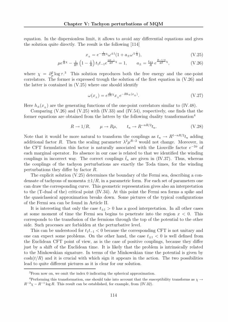
Chapter V: Tachyon perturbations of MQM
equation. In the dispersionless limit, it allows to avoid any differential equations and givesthe solution quite directly. The result is the following [114]
x± = e−1
2Rχω±1(1 + a±ω
∓ 1R ), (V.25)
µe1Rχ − 1
R2
(
1 − 1R
)
t1t−1e2R−1
R2 χ = 1, a± = t∓1
Re
R−1/2
R2 χ, (V.26)
where χ = ∂2µ log τ .3 This solution reproduces both the free energy and the one-point
correlators. The former is expressed trough the solution of the first equation in (V.26) andthe latter is contained in (V.25) where one should identify
ω(x±) = e1
2Rχx±e
−Rh±(x±). (V.27)
Here h±(x±) are the generating functions of the one-point correlators similar to (IV.48).Comparing (V.26) and (V.25) with (IV.33) and (IV.54), respectively, one finds that the
former equations are obtained from the latters by the following duality transformation4
R → 1/R, µ→ Rµ, tn → R−nR/2tn. (V.28)
Note that it would be more natural to transform the couplings as tn → R1−nR/2tn addingadditional factor R. Then the scaling parameter λ2µR−2 would not change. Moreover, inthe CFT formulation this factor is naturally associated with the Liouville factor e−2φ ofeach marginal operator. Its absence in our case is related to that we identified the windingcouplings in incorrect way. The correct couplings tn are given in (IV.37). Thus, whereasthe couplings of the tachyon perturbations are exactly the Toda times, for the windingperturbations they differ by factor R.
The explicit solution (V.25) determines the boundary of the Fermi sea, describing a con-densate of tachyons of momenta ±1/R, in a parametric form. For each set of parameters onecan draw the corresponding curve. This geometric representation gives also an interpretationto the (T-dual of the) critical point (IV.34). At this point the Fermi sea forms a spike andthe quasiclassical approximation breaks down. Some pictures of the typical configurationsof the Fermi sea can be found in Article II.
It is interesting that only the case t±1 > 0 has a good interpretation. In all other casesat some moment of time the Fermi sea begins to penetrate into the region x < 0. Thiscorresponds to the transfusion of the fermions through the top of the potential to the otherside. Such processes are forbidden at the perturbative level.
This can be understood for t1t−1 < 0 because the corresponding CFT is not unitary andone can expect some problems. On the other hand, the case t±1 < 0 is well defined fromthe Euclidean CFT point of view, as is the case of positive couplings, because they differjust by a shift of the Euclidean time. It is likely that the problem is intrinsically relatedto the Minkowskian signature. In terms of the Minkowskian time the potential is given bycosh(t/R) and it is crucial with which sign it appears in the action. The two possibilitieslead to quite different pictures as it is clear for our solution.
3From now on, we omit the index 0 indicating the spherical approximation.4Performing this transformation, one should take into account that the susceptibility transforms as χ→
R−2χ−R−1 logR. This result can be established, for example, from (IV.32).
114

§2 Thermodynamics of tachyon perturbations
2 Thermodynamics of tachyon perturbations
2.1 MQM partition function as τ-function
In the previous section we showed that the tachyon perturbations with momenta as in thecompactified Euclidean theory are described by the constrained Toda hierarchy. Hence, theyare characterized by a τ -function. What is the physical interpretation of this τ -function? In[92] it was identified as the generating functional for scattering amplitudes of tachyons. Onthe other hand, since the tachyon spectrum coincides with that of the theory at finite tem-perature, it is tempting to think that the theory possesses a thermodynamical interpretation.Then the τ -function could be seen as the partition function of the model.
Although expected, the existence of the thermodynamical interpretation is not guaran-teed because the system is formulated in the Minkowskian time and except the coincidenceof the spectra there is no reference to a temperature. However, we will show that it doesexist at least for the case of the Sine-Liouville perturbation [117]. In the following we willaccept this point of view and will show that the τ -function is indeed the grand canonicalpartition function at temperature T = 1/β. In the spherical limit this was done in [114, 117]and we will present that derivation in the next paragraph. Here we prove the statement to allorders in perturbation theory following the paper [118] (Article IV) which will be discussedin chapter VI.
The grand canonical partition function is defined as follows
Z(µ, t) = exp[∫ ∞
−∞dE ρ(E) log
(
1 + e−1hβ(µ+E)
)
]
, (V.29)
where ρ(E) is the density of states. It can be found by confining the system in a box ofsize ∼
√Λ similarly as it was done in section III.2.4. The difference is that now we work in
the light cone representation. Therefore, one should generalize the quantization condition(III.38). The generalization is given by
[SΨ](√
Λ) = Ψ(√
Λ) (V.30)
so that one identifies the scattered state with the initial one at the wall. Then from theexplicit form of the perturbed wave function (V.7) with (V.10) one finds [118]
ρ(E) =log Λ
2π− 1
2π
dφ(E)
dE. (V.31)
Integrating by parts in (V.29), closing the contour in the upper half plane and taking theintegral by residues of the thermal factor, one obtains [118]
Z(µ, t) =∏
n≥0
exp
[
iφ
(
ihn+ 1
2
R− µ
)]
. (V.32)
On the other hand, the zero mode of the perturbing phase is actually equal to the zeromode of the dressing operators (II.98). Hence it is expressed through the τ -function as in
115

Chapter V: Tachyon perturbations of MQM
(II.103). Since the shift in the discrete parameter s is equivalent to an imaginary shift ofthe chemical potential µ, this formula reads
eihφ(−µ) =
τ0(
µ+ i h2R
)
τ0(
µ− i h2R
) . (V.33)
Comparing this result with (V.32), one concludes that
Z(µ, t) = τ0(µ, t). (V.34)
2.2 Integration over the Fermi sea: free energy and energy
As always, in the dispersionless limit one can give to all formulae clear geometrical inter-pretation. Moreover, this limit allows to obtain additional information about the system.Namely, in this paragraph we show how such thermodynamical quantities as the free energyand the energy of 2D string theory perturbed by tachyon sources are restored from the Fermisea of the singlet sector of MQM. This was done in the work [117] (Article III).
Since in the classical limit the profile of the Fermi sea uniquely determines the stateof the free fermion system, it encodes all the interesting information. Indeed, in the fullquantum theory the expectation value of an operator is given by its quantum average in thegiven state. Its classical counterpart is the integral over the phase space of the correspondingfunction multiplied by the density of states. For the free fermions the density of states equals1 or 0 depending on either the phase space point is occupied or not. As a result, the classicalvalue of an observable O is represented by its integral over the Fermi sea
< O >=1
2π
∫ ∫
Fermi sea
dx+dx− O(x+, x−). (V.35)
Now the description in terms of the dispersionless Toda hierarchy comes into the game.We saw that the tachyon perturbation give rise to the canonical transformation from x± tothe set of variables (E, logω). The explicit map is given by (V.25) for the simplest case ofthe Sine–Liouville theory and it is easily extended to the general case of a potential of degreen. Due to this the measure in (V.35) can be rewritten in terms of E and ω. As a result, onearrive at the following formula
∂µ < O >= − 1
2π
ω+
(µ)∫
ω− (µ)
dω
ωO(x+(ω, µ), x−(ω, µ)). (V.36)
The limits of integration are defined by the cut-off Λ. How they can be found is explainedin detail in Article III.
The result (V.36) is rather general. We applied it to the main two observables which arethe energy and the number of particles. They were already defined in (III.27) and (III.26)for the case of the ground state. In a more general case they are written as integrals (V.35)
116

§2 Thermodynamics of tachyon perturbations
with O = −x+x− and O = 1, correspondingly. In these two cases the integral (V.36) iseasily calculated leading to
∂µN = − 1
2πlog Λ − 1
2πRχ, (V.37)
∂µE =1
2πe−
1Rχ
(1 + a+a−)(
log Λ +1
Rχ)
− 2a+a−
+R
2π(t1 + t−1)Λ
1/2R, (V.38)
where the second equation is valid for the Sine–Liouville perturbation. Using (V.26), onecan integrate (V.38) and obtain an expression for the energy of the system [117].
To reproduce the free energy, note that in the grand canonical ensemble it is related tothe number of particles through
N = ∂F/∂µ, (V.39)
where we changed our notations assuming the usual thermodynamical definition of the freeenergy at the temperature T
F = −T logZ. (V.40)
Comparing (V.39) and (V.37), one obtains the expected result
F = − 1
βlog τ. (V.41)
In particular, the temperature is associated with 1/β. Integrating the equation for thesusceptibility χ, one can get an explicit representation for the free energy. It coincides withthe T-dual transform of (IV.31).
2.3 Thermodynamical interpretation
In Article III we proved that the derived expressions for the energy and free energy allowa thermodynamical interpretation. This is not trivial because there are two definitions ofthe macroscopic energy. One of them is the sum of microscopic energies of the individualparticles which is expressed as an integral over the phase space. We used this definition inthe previous paragraph. Another definition follows from the first law of thermodynamicswhich relates the energy, free energy and entropy
S = β(E − F ). (V.42)
It allows to express the energy and entropy as derivatives of the free energy with respect tothe temperature
E =∂(βF )
∂β, S = −∂F
∂T. (V.43)
To have a consistent thermodynamical interpretation, the two definitions must give the sameresult. It is a very non-trivial check, although very simple from the technical point of view.All that we need is to differentiate the free energy, which is given through the solution ofthe algebraic equation (V.26), and check that the result coincides with the one obtainedintegrating (V.38).
117

Chapter V: Tachyon perturbations of MQM
However, there are two important subtleties. The first one is that the first law is formu-lated in terms of the canonical free energy F rather than for its grand canonical counterpartF . This is in agreement with the fact that it is the canonical free energy that is interpretedas the partition function of string theory. Thus, it is F that carries an information aboutproperties of the string background. Due to this one should pass to the canonical ensemble
F = F − µ∂F∂µ
. (V.44)
If the first subtlety answers to the question ”what to differentiate?”, the second oneconcerns the problem ”how to differentiate?”. The problem is what parameters should beheld fixed when one differentiates with respect to the temperature. First, this may be eitherµ or N . It is important to make the correct choice because they are non-trivial functionsof each other. Since we are working in the canonical ensemble, it is natural to take N asindependent variable. Besides, one should correctly identify the coupling λ and the cut-offΛ. Their definition can involve R and, thus, contribute to the result.
It turns out [117] that the coupling and cut-off that we have chosen are already the correctones. By direct calculation it was shown that the thermodynamical relations (V.43), wherethe derivatives are taken with N , λ and Λ fixed, are indeed fulfilled. Thus, the 2D stringtheory perturbed by tachyons of momenta ±i/R in Minkowskian spacetime has a consistentinterpretation as a thermodynamical system at temperature T = 1/(2πR).
This result also answers to the question risen in section IV.2.3: what variable should beassociated with the temperature? Our analysis definitely says that this is the parameterR. We do not need to introduce such notion as ”temperature at the wall” [29, 30, 34].The differentiation is done directly with respect to the compactification radius. Also thissupports the idea that in the dual picture a black hole background should exist for anycompactification radius, at least in the interval 1 < R < 2.
The first law of thermodynamics (V.42) or the relations (V.43) allow to calculate theentropy. It vanishes in the absence of perturbations when λ = 0 but it is a complicatedfunction in the general case. It would be quite interesting to understand the microscopicorigin of this entropy. In other words, we would like to find the microscopic degrees offreedom giving rise to non-vanishing entropy. However, we have not found the solutionyet. The problem is that a state of the system is uniquely characterized by the profileof the Fermi sea and there is only one profile described by our solution for each state.The only possibility which we found to obtain different microscopic states is to associatethem with different positions in time of the same Fermi sea. Although the Fermi sea istime-dependent, all macroscopic thermodynamical quantities do not depend on time. Thus,different microscopic states would define the same macroscopic state. This idea is supportedalso by the fact that the entropy vanishes only if the Fermi sea is stationary. However, wehave not succeeded to get the correct result for the entropy from this picture.
It is tempting to claim that the obtained thermodynamical quantities describe after theduality transformation (V.28) the thermodynamics of winding perturbations and their stringbackgrounds. This is, of course, true for the free energy. However, it is not clear whether theenergy and entropy are dual in the two systems. For example, it is not understood even howto define the energy of a winding condensate. Nevertheless, if we assume that our resultscan be related to the backgrounds generated by windings, this gives a plausible picture. For
118
§2 Thermodynamics of tachyon perturbations
example, the non-vanishing entropy can be explained with the existence of a black hole.Our results concern arbitrary radius R and cosmological constant µ. When the latter goes
to zero, which corresponds to the black hole point according to [35], the situation becomeslittle bit special. Namely, the logarithmic term ξ−2 log(Λξ) in the free energy disappears,whereas it is present in the energy and entropy. This term is the leading one. Therefore,both the energy and entropy are much larger than the free energy. This can explain thepuzzle that, on the one hand, the dilaton gravity predicts vanishing free energy and, onthe other hand, the matrix model gives a non-vanishing result. Our approach shows that itdoes not vanish but it is negligible in comparison with other quantities so that in the mainapproximation the law S = βE is valid.
119

Chapter V: Tachyon perturbations of MQM
3 Backgrounds of 2D string theory
We introduced the tachyon perturbations as one of the ways to change the background of2D string theory. How exactly does the background corresponding to non-vanishing tn look?Any background has two types of characteristics, local and global. The local structure iscaptured by values of the background fields which are the metric, dilaton and tachyon. Butalso backgrounds can differ by their global structure. Of course, the introduction of tachyoncouplings in the way described in section 1 changes the value of the tachyon field. But maybe it can change also some other properties of the background? We tried to answer thisquestion in the work [119] (Article V).
3.1 Local properties
First, let us analyze the local properties of the background obtained by a perturbation of thetype (V.7). We will restrict ourselves to the spherical approximation. Then the backgroundis uniquely determined by the profile of the Fermi sea. Thus, we should find the backgroundfields using a given profile as a starting point.
As we could see above, the fermionic representation used to introduce the perturbationsis very convenient for the solution of many problems. However, it is not suited to discussthe target space phenomena. For these purposes we should use a collective field theory.We have already given an introduction to such theory constructed by Das and Jevicki (seesection III.3). It turns out that it can be used to extract an information about the stringbackground.
In fact, we have already done this for the simplest case of the linear dilaton backgroundwhich was obtained from the ground state of the system of free fermions of the singlet sectorof MQM. In particular, we identified the tachyon field with fluctuations of the matrix modeldensity of eigenvalues around the ground state. We expect that this identification holds tobe true also in more complicated cases. All that we need to obtain another background isto replace the background value of the density by a new function obtained from the exactform of the deformed profile of the Fermi sea. In this way one can find an effective actionfor the tachyon. Then our idea was to compare this action with the similar action obtainedas a low-energy limit of string theory discussed in section I.3.
One should say that our analysis uses a simplified version of the relation between the Das–Jevicki collective theory and 2D string theory. The exact relation requires identification ofthe tachyon with the loop operator rather than with the density (see (III.78)). The formeris the Fourier transform of the latter, so that the relation between the density and thestring tachyon is non-local. For the simplest case of the ground state, the analysis can benevertheless completed. For the time-dependent backgrounds, we are going to consider, thesituation becomes much more complicated. We do not know how to find the exact relationin this case. Instead we neglect the Liouville and sine-Liouville terms in the equation for thetachyon field and identify this field with the fluctuations of the density. And it is already aremarkable fact that in this approximation the problem can be solved exactly.
First, we obtain an effective action for the density fluctuations from the Das–Jevickitheory. For this it is sufficient to make the substitution (III.61) into the background inde-pendent effective action (III.54). However, in contrast to the previous case, the background
120
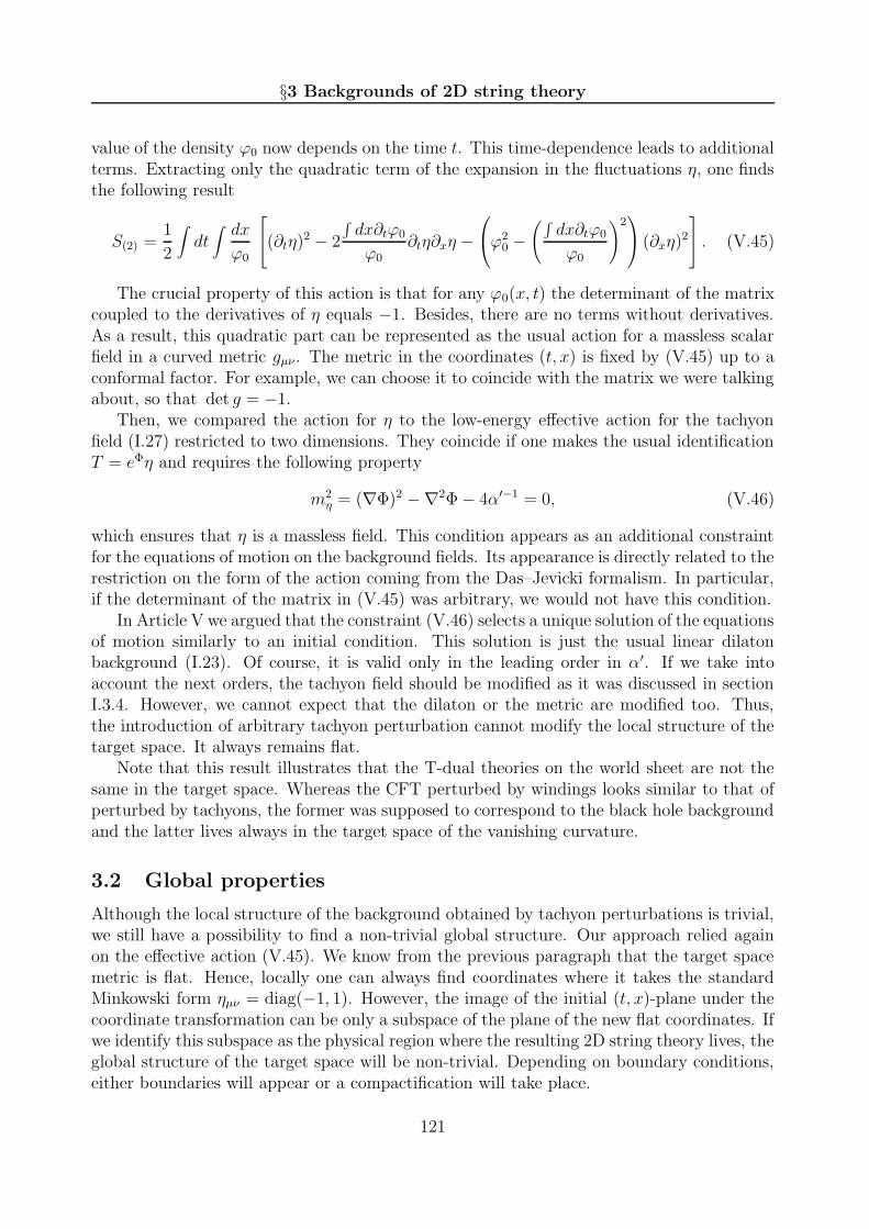
§3 Backgrounds of 2D string theory
value of the density ϕ0 now depends on the time t. This time-dependence leads to additionalterms. Extracting only the quadratic term of the expansion in the fluctuations η, one findsthe following result
S(2) =1
2
∫
dt∫ dx
ϕ0
(∂tη)2 − 2
∫
dx∂tϕ0
ϕ0∂tη∂xη −
ϕ20 −
(∫
dx∂tϕ0
ϕ0
)2
(∂xη)2
. (V.45)
The crucial property of this action is that for any ϕ0(x, t) the determinant of the matrixcoupled to the derivatives of η equals −1. Besides, there are no terms without derivatives.As a result, this quadratic part can be represented as the usual action for a massless scalarfield in a curved metric gµν. The metric in the coordinates (t, x) is fixed by (V.45) up to aconformal factor. For example, we can choose it to coincide with the matrix we were talkingabout, so that det g = −1.
Then, we compared the action for η to the low-energy effective action for the tachyonfield (I.27) restricted to two dimensions. They coincide if one makes the usual identificationT = eΦη and requires the following property
m2η = (∇Φ)2 −∇2Φ − 4α′−1 = 0, (V.46)
which ensures that η is a massless field. This condition appears as an additional constraintfor the equations of motion on the background fields. Its appearance is directly related to therestriction on the form of the action coming from the Das–Jevicki formalism. In particular,if the determinant of the matrix in (V.45) was arbitrary, we would not have this condition.
In Article V we argued that the constraint (V.46) selects a unique solution of the equationsof motion similarly to an initial condition. This solution is just the usual linear dilatonbackground (I.23). Of course, it is valid only in the leading order in α′. If we take intoaccount the next orders, the tachyon field should be modified as it was discussed in sectionI.3.4. However, we cannot expect that the dilaton or the metric are modified too. Thus,the introduction of arbitrary tachyon perturbation cannot modify the local structure of thetarget space. It always remains flat.
Note that this result illustrates that the T-dual theories on the world sheet are not thesame in the target space. Whereas the CFT perturbed by windings looks similar to that ofperturbed by tachyons, the former was supposed to correspond to the black hole backgroundand the latter lives always in the target space of the vanishing curvature.
3.2 Global properties
Although the local structure of the background obtained by tachyon perturbations is trivial,we still have a possibility to find a non-trivial global structure. Our approach relied againon the effective action (V.45). We know from the previous paragraph that the target spacemetric is flat. Hence, locally one can always find coordinates where it takes the standardMinkowski form ηµν = diag(−1, 1). However, the image of the initial (t, x)-plane under thecoordinate transformation can be only a subspace of the plane of the new flat coordinates. Ifwe identify this subspace as the physical region where the resulting 2D string theory lives, theglobal structure of the target space will be non-trivial. Depending on boundary conditions,either boundaries will appear or a compactification will take place.
121

Chapter V: Tachyon perturbations of MQM
(ω, t)ω∼
sing(t)ω
(ω, t)p
ω
(ω, t)ϕ0
(ω, t)p∼
x
p
Fig. V.1: The Fermi sea of the perturbed MQM. Its boundary is defined by a two-valuedfunction with two branches parameterized by p(ω, t) and p(ω, t). The background field ϕ0
coincides with the width of the Fermi sea.
Thus, the global structure of the target space is determined by the transformation tothe flat coordinates. Up to a conformal factor it can be deduced from the action (V.45).Unfortunately, we are not able to find the transformation for arbitrary ϕ0(x, t) which isa solution of the classical equations followed from (III.54). Nevertheless, this task wasaccomplished for the integrable perturbations generated by the potential (V.11) [119].
In this case we have the description in terms of Toda hierarchy which allows to find theexact form of the profile of the Fermi sea. It is given by a generalization of (V.25). For theperturbing potentials of degree n, it is represented in the following parametric form
p(ω, t) =n∑
k=0ak sinh
[(
1 − kR
)
ω + kRt + αk
]
,
x(ω, t) =n∑
k=0ak cosh
[(
1 − kR
)
ω + kRt + αk
]
,(V.47)
where ω is now the logarithm of the shift operator from the previous sections. The functionp(x) is two valued. The density ϕ0(x, t) is given by the difference of the two branches. How-ever, it is more convenient for us to work in the ω-parameterization. Then the first branch isgiven by p(ω, t) in (V.47), whereas the second one is obtained as p(ω, t) = p(ω(ω, t), t) whereω(ω, t) is defined as a parameter mirror to ω (see fig. V.1). In terms of these functions thequadratic part of the effective action (V.45) is rewritten as follows
S(2) =∫
dt∫
dx
p− p
[
(∂tη)2 + (p+ p)∂tη∂xη + pp(∂xη)
2]
. (V.48)
In Article V we showed the following coordinate transformation brings the action (V.48)to the standard form with the kinetic term written in the Minkowski metric ηµν
τ = t− ω + ω
2, q =
ω − ω
2. (V.49)
The change of coordinates (V.49) is remarkably simple and has a transparent interpretation.It associates the target space light-cone coordinates τ ± q with the parameters of incomingand outgoing tachyons, t − ω and t − ω. For the ground state, when the perturbation isabsent, the mirror parameter is ω = −ω so that we return to the simple situation describedin section III.3.2.
122

§3 Backgrounds of 2D string theory
The coordinates (V.49) are not necessarily the ones where the metric is trivial. Theaction in two dimensions possesses the remaining gauge symmetry allowing to make theconformal transformations
(τ, q) −→ (u(t− ω), v(t− ω)) . (V.50)
We were not able to fix the functions u and v. However, we argued that since the conformalmaps preserve the causal structure, some conclusions can be made neglecting this ambiguity.
Once the transformation (V.49) was found, it is possible to study the exact form of theresulting target space. This was done for the simplest case of the Sine–Liouville perturbationwhen n = 1 in (V.47). The result crucially depends on the parameter R. There are 3 differentregions. When R ≥ 1 nothing special happens and the target space coincides with the wholeplane. For 1/2 < R < 1 the target space is deformed so that asymptotically it can beconsidered as two conic regions |τ/q| < 2R − 1. When we approach the origin we find thattwo cones are smoothly glued along a finite interval of length
∆ = 2R log[
R
1 − R
a0
a1
]
. (V.51)
For R < 1/2 the picture is similar to the previous case but the time and space coordinatesare exchanged so that the picture should be rotated by 90.
It is interesting that this target space exhibits the same singularity as the one we found inthe analysis of the free energy and the perturbed Fermi sea. The singularity appears when thelength ∆ vanishes so that the two conic regions separate from each other. The correspondingcritical value of µ is exactly the same as (IV.34) after the duality transformation (V.28).
The obtained conic spacetimes possess boundaries. Therefore, some boundary conditionsshould be imposed on the fields propagating there. We discussed them and their physicalinterpretation in detail in Article V. We proposed three possible boundary conditions: thevanishing boundary conditions, periodic and twisted periodic ones. Which conditions arerelevant for each case remained an unsolved problem.
Another unsolved problem is related to the thermodynamical interpretation. We sawthat the perturbed 2D string theory in the Minkowskian spacetime can be considered as atheory at finite temperature T = 1/(2πR). It would be very interesting to reproduce thisresult from the analysis of quantum field theory in the target space obtained above. It is wellknown that boundaries or a compactification with varying radius can give rise to a thermalspectrum of observed particles [120]. Therefore, our picture seems to be reasonable. How-ever, the problem is technically difficult and complicated by the ambiguity in the conformaltransformation (V.50).
The obtained results shed light on some properties of 2D string theory with tachyoncondensation, but they are not related (at least directly) to the most interesting problemof 2D string theory in curved backgrounds. The latter should be obtained by windingperturbations. Although from the CFT point of view they are not much different from thetachyon perturbations, in the MQM framework their description is much more complicated.For the tachyon modes there is a powerful free fermion representation and, as a consequence,the Das–Jevicki collective field theory. It is this formulation that allowed us to get someinformation about the string target space. For windings there is no analog of this formalismand how to show, for example, that the winding perturbations of MQM correspond to theblack hole background is still an open problem.
123


Chapter VI
MQM and Normal Matrix Model
In this chapter we present the next work included in this thesis [118] (Article IV). It stays alittle bit aside the main line of our investigation. Nevertheless it opens one more aspect of 2Dstring theory in non-trivial backgrounds and its Matrix Quantum Mechanical formulation,in particular. This work establishes an equivalence of the tachyonic perturbations of MQMdescribed in the previous chapter with the so called Normal Matrix Model (NMM). Thismodel appears in the study of various physical and mathematical problems. Therefore,before to discuss our results, we will briefly describe the main features of NMM and therelated issues.
1 Normal matrix model and its applications
1.1 Definition of the model
The Normal Matrix Model was first introduced in [121, 122]. It is a statistical model ofrandom complex matrices which commute with their conjugates
[Z,Z†] = 0. (VI.1)
As usual, its partition function is represented as the matrix integral
ZN =∫
dν(Z,Z†) exp[
−1
hW (Z,Z†)
]
, (VI.2)
where the measure dν is a restriction of the usual measure on the space of all N×N complexmatrices to those that satisfy the relation (VI.1). For our purposes we introduced explicitlythe Planck constant at the place of N . They are supposed to be related in the large N limitwhich is obtained as N → ∞, h→ 0 with hN fixed.
The potentials which can be considered are quite general. We will be interested especiallyin the following type of potentials
WR(Z,Z†) = tr (ZZ†)R − hγ tr log(ZZ†) − trV (Z) − tr V (Z†). (VI.3)
whereV (Z) =
∑
k≥1
tkZk, V =
∑
k≥1
t−kZ†k. (VI.4)
125

Chapter VI: MQM and Normal Matrix Model
The probability measure with such a potential depends on several parameters. These areR, γ and two sets of tn and t−n. The latter are considered as coupling constants becausethe dependence on them of the partition function contains an information about correlatorsof the matrix operators trZk. The other two parameters R and γ are just real numberscharacterizing the particular model.
The partition function (VI.2) resembles the two-matrix model studied in section II.4.Similarly to that model, one can do the reduction to eigenvalues. The difference with respectto 2MM is that now the eigenvalues are complex numbers and the measure takes the form
dν(Z,Z†) =1
N ![dΩ]SU(N)
N∏
k=1
d2zk |∆(z)|2. (VI.5)
Thus, instead of two integrals over real lines one has one integral over the complex plane.Despite this difference, one can still introduce the orthogonal polynomials and the relatedfermionic representation. Then, repeating the arguments of section II.5.7, it is easy to provethat the partition function (VI.2) is a τ -function of Toda hierarchy as well. For the case ofR = 1 this was demonstrated in [67] and for generic R the proof can be found in appendixA of Article IV. In fact, for the particular case R = 1 (and γ = 0) it was proven [68] thatNMM and 2MM coincide in the sense that they possess the same free energy as function ofthe coupling constants. Nevertheless, their interpretation remains different.
The eigenvalue distribution of NMM in the large N limit is also similar to the picturearising in 2MM and shown on fig. II.7. The eigenvalues fill some compact spots on a two-dimensional plane. The only difference is that earlier this was the plane formed by realeigenvalues of the two matrices, and now this is the complex z-plane. Therefore, the widthof the spots does not have anymore a direct interpretation in terms of densities. Instead,the density inside the spots for a generic potential can be non-trivial. For example, for thepotential (VI.3) it is given by
ρ(z, z) =1
π∂z∂zWR(z, z) =
R2
π(zz)R−1. (VI.6)
For R = 1 where NMM reduces to 2MM, we return to the constant density.
1.2 Applications
Recently, the Normal Matrix Model found various physical applications [123, 124]. Mostremarkably, it describes phenomena whose characteristic scale differs by a factor of 109.Whereas some of these phenomena are purely classical, another ones are purely quantum.
Quantum Hall effect
First, we mention the relation of NMM to the Quantum Hall effect [125]. There one considerselectrons on a plane in a strong magnetic field B. The spectrum of such system consists fromLandau levels. Even if the magnetic field is not uniform, the lowest level is highly degenerate.The degeneracy is given by the integer part of the total magnetic flux 1
2πh
∫
B(z)d2z, andthe one-particle wave functions at this level have the following form
ψn(z) = Pn(z) exp
(
−W (z)
2h
)
. (VI.7)
126

§1 Normal matrix model and its applications
Here W (z) is related to the magnetic field through B(z) = 12∆W (z) and Pn(z) are holomor-
phic polynomials of degree n with the first coefficient normalized to 1.Usually, one is interested in situations when all states at the lowest level are occupied.
Then the wave function of N electrons is the Slater determinant of the one-particle wavefunctions (VI.7). Hence, it can be represented as
ΨN(z1, . . . , zN ) =1√N !
∆(z) exp
(
− 1
2h
N∑
k=1
W (zk)
)
. (VI.8)
Its norm coincides with the probability measure of NMM. Therefore, the partition function(VI.2) appears in this picture as a normalization factor of the N -particle wave function
ZN =∫ N∏
k=1
d2zk |ΨN(z1, . . . , zN)|2. (VI.9)
Similarly, the density of electrons can be identified with the eigenvalue density and the sameis true for their correlation functions.
Due to this identification, in the quasiclassical limit the study of eigenvalue spots isequivalent to the study of electronic droplets. In particular, varying the matrix modelpotential one can investigate how the shape of the droplets changes with the magnetic field.At the same time, varying the parameter hN one examines its evolution with increasing thenumber of electrons.
Note that although we discussed the semiclassical regime, the system remains intrinsicallyquantum. The reason is that all electrons under consideration occupy the same lowest level,whereas the usual classical limit implies that higher energy levels are most important.
Laplacian growth and interface dynamics
It was shown [125] that when one increases the number of electrons the semiclassical dropletsfrom the previous paragraph evolve according to the so called Darcy’s law which is alsoknown as Laplacian growth. It states that the normal velocity of the boundary of a dropletoccupying a simply connected domain D is proportional to the gradient of a scalar function
1
h
δ~n
δN∼ ~∇ϕ(z), (VI.10)
which is harmonic outside the droplet and vanishes at its boundary
∆ϕ(z, z) = 0, z ∈ C\D, ϕ(z, z) = 0, z ∈ ∂D. (VI.11)
In the matrix model this function appears as the following correlator
ϕ(z, z) = h⟨
tr(
log(z − Z)(z − Z†))⟩
. (VI.12)
It turns out that exactly the same law governs the dynamics of viscous flows. Thisphenomenon appears when an incompressible fluid with negligible viscosity is injected intoa viscous fluid. In this case the harmonic function ϕ has a concrete physical meaning. It isidentified with the pressure in the viscous fluid ϕ = −P . In fact, the Darcy’s law is only
127

Chapter VI: MQM and Normal Matrix Model
an approximation to a real evolution. Whereas the condition P = 0 in the incompressiblefluid is reasonable, the vanishing of the pressure at the interface is valid only when thesurface tension can be neglected. This approximation fails to be true when the curvature ofthe boundary becomes large. Then the dynamics is unstable and the incompressible fluiddevelops many fingers so that its shape looks as a fractal. This is known as the Saffman–Taylor fingering.
NMM provides a mathematical framework for the description of this phenomenon. Fromthe previous discussion it is clear that it describes the interface dynamics in the large N limit.In this approximation the singularity corresponding to the described instabilities arises whenthe eigenvalue droplet forms a spike which we encountered already in the study of the Fermisea of MQM (section V.1.4). We know that at this point the quasiclassical approximationis not valid anymore. But the full quantum description still exists. Therefore, it is naturalto expect that the fingering, which is a feature of the Laplacian growth, can be captured byincluding next orders of the 1/N expansion of NMM.
Complex analysis
The Darcy’s law (VI.10) shows that there is a relation between NMM and several problems ofcomplex analysis. Indeed, on the one hand, it can be derived from NMM as the evolution lawof eigenvalue droplets and, on the other hand, it gives rise to a problem to find a harmonicfunction given by the domain in the complex plane. The latter problem appears in differentcontexts such as the conformal mapping problem, the Dirichlet boundary problem, and the2D inverse potential problem [111]. For instance, if we fix the asymptotics of ϕ(z, z) requiringthat
ϕ(z, z) ∼z→∞
log |z|, (VI.13)
the solution of (VI.11) is unique and given by the holomorphic function ω(z)
ϕ(z, z) = log |ω(z)|, (VI.14)
which maps the domain D onto the exterior of the unit circle and has infinity as a fixedpoint. To find such a function is the content of the conformal mapping problem.
Further, the Dirichlet boundary problem, which is to find a harmonic function f(z, z) inthe exterior domain given a function g(z) on the boundary of D, is solved in terms of theabove defined ω(z). The solution is given by
f(z, z) = − 1
πi
∮
∂Dg(ζ)∂ζG(z, ζ)dζ, (VI.15)
where the Green function is
G(z, ζ) = log
∣
∣
∣
∣
∣
ω(z) − ω(ζ)
ω(z)ω(ζ) − 1
∣
∣
∣
∣
∣
. (VI.16)
In turn, ω(z) is obtained as the holomorphic part of G(z,∞).Finally, the inverse potential problem can be formulated as follows. Let the domain D
is filled by a charge spread with some density. The charge creates an electrostatic potentialwhich is characterized by two functions ϕ+ and ϕ− defined in the interior and exterior
128
§1 Normal matrix model and its applications
domains, respectively. They and their derivatives are continuous at the boundary ∂D. Theproblem is to restore the form of the charged domain given one of these functions. At thesame time, when both of them are known the task can be trivially accomplished. Therefore,the problem is equivalent to the question how to restore ϕ− from ϕ+. Its relation to theDirichlet boundary problem becomes now evident because, since ϕ− is harmonic, it is given(up to a logarithmic singularity at infinity) by the formula (VI.15) with g = ϕ+.
Thus, we see that the Normal Matrix Model provides a unified description for all thesemathematical and physical problems. The main lesson which we learn from this is that all ofthem possess a hidden integrable structure revealed in NMM as Toda integrable hierarchy.
129

Chapter VI: MQM and Normal Matrix Model
2 Dual formulation of compactified MQM
2.1 Tachyon perturbations of MQM as Normal Matrix Model
In section V.1 we showed how to introduce tachyon perturbations into the Matrix QuantumMechanical description of 2D string theory. Although it is still the matrix model framework,we have done it in an unusual way. Instead to deform the matrix model potential, we havereduced MQM to the singlet sector and changed there the one-fermion wave functions. Onecan ask: can the resulting partition function be represented directly as a matrix integral?
In fact, the tachyon perturbations of MQM are quite similar to the perturbations of thetwo-matrix model. First, they are both described by Toda hierarchy. Second, the phasespace of MQM looks as the eigenvalue (x, y) plane of 2MM. In the former case the fermionsassociated with the time dependent eigenvalues fill the non-compact Fermi sea, whereas inthe latter case they fill some spots. If the 2MM potential is unstable like the inverse oscillatorpotential −x+x− , the spots will be non-compact as well. Thus, it is tempting to identify thetwo pictures.
Of course, MQM is much richer theory than 2MM and one may wonder how such differenttheories could be equivalent. The answer is that we have restricted ourselves just to alittle sector of MQM. First, we use the restriction to the singlet sector and, second, we areinterested only in the scattering processes. This explains why only two matrices appear.They are associated with in-coming and out-going states or, in other words, with M(−∞)and M(∞).
But it is easy to guess that the idea to identify MQM perturbed by tachyons with 2MMdoes not work. Indeed, the partition function of 2MM is a τ -function of Toda hierarchywhen it is considered in the canonical ensemble. Therefore, one should find a representationof the grand canonical partition function of MQM which has a form of a canonical one. Sucha representation does exist and is given by (V.32). But it implies a discrete equally spacedenergy spectrum. It is evident for the system without perturbations where the partition
function is a product of R-factors (V.6) corresponding to En = −µ + ihn+ 1
2
R. However,
it is difficult to obtain such a spectrum from two hermitian matrices. Moreover, one canshow that their diagonalization would produce Vandermonde determinants of monomials ofincorrect powers.
All these problems are resolved if one considers another model of two matrices which is theNMM. In the work [118] (Article IV) we proved that the grand canonical partition functionof MQM with tachyon perturbations coincides with a certain analytical continuation of thecanonical partition function of NMM. Thus, NMM can be regarded as a new realization of2D string theory perturbed by tachyons.
Our proof is based on the fact that the two partition functions are τ -functions of Todahierarchy. Therefore, it is enough to show that they are actually the same τ -function. Thisfact follows from the coincidence of either string equations or the initial conditions given bythe non-perturbed partition functions. Finally, one should correctly identify the parametersof the two models.
We suggested two ways to identify the parameters. First, let us consider NMM given bythe integral (VI.2) with the potential (VI.3) where γ = 1
2(R−1)+ α
h. We denote its partition
130

§2 Dual formulation of compactified MQM
function by ZNMM
h (N, t, α). Then there is the following identification
Zh(µ, t) = limN→∞
ZNMM
ih (N, t, Rµ− ihN). (VI.17)
We proved this result by direct comparison of two non-perturbed partition functions. Theircoincidence is a consequence of the fact that the normalization coefficients (II.59) of theorthogonal polynomials in NMM coincide with the reflection coefficients (V.6)
hn(α) ∼ R(
−ihn+ 12
R− i
α
R
)
. (VI.18)
Note that although the identification (VI.17) involves a large N limit, the relation isvalid to all orders in the genus expansion. This is because N enters non-trivially through theparameter α. Actually, N appears always in a combination with µ. This is needed becausethe discrete charge of the τ -function is identified either with iµ or with N .
This fact hints that there should exist another way to match the two models in whichthese parameters are directly identified with each other. It is given by the second modelproposed in Article IV
Zh(µ, t) = ZNMM
ih (− i
hRµ, t, 0). (VI.19)
The equivalence of the two partition functions is proven in the same way as earlier. Thissecond model is simpler than the first one because it does not involve the large N limit andone can compare the 1/N expansion of NMM directly with the 1/µ expansion of MQM.
2.2 Geometrical description in the classical limit and duality
The relation of the perturbed MQM and NMM is a kind of duality. Most explicitly, this isseen in the classical limit where the both models have a geometrical description in terms ofincompressible liquids. In the case of MQM, it describes the Fermi sea in the phase spaceparameterized by two real coordinates x± , whereas in the case of NMM the liquid correspondsto the compact eigenvalue spots on the complex z-plane. Thus, the first conclusion is thatthe variables of one model are obtained from the variables of the other by an analyticalcontinuation. The exact relation is the following
x+ ↔ zR, x− ↔ zR. (VI.20)
It relates all correlators in the two models if simultaneously one substitutes h → ih andN = −iRµ/h.
In particular, the analytical continuation (VI.20) replaces the non-compact Fermi sea ofMQM by a compact eigenvalue spot of NMM. We have already discussed in the context ofMQM that the profile of the Fermi sea is determined by the solution x−(x+) (or or its inversex+(x−) depending on what asymptotics is considered) of the string equation (V.24). Thesame is true for the boundary of the NMM spot. Since the two models coincide, the stringequations are also the same up to the change (VI.20). Nevertheless, they define differentprofiles. The MQM equation gives a non-compact curve and the NMM equation leads to acompact one. For example, when all tn = 0 the two equations read
x+x− = µ, (zz)R = hN/R (VI.21)
131

Chapter VI: MQM and Normal Matrix Model
!"!"!"!"!"!"!"!!"!"!"!"!"!"!"!!"!"!"!"!"!"!"!!"!"!"!"!"!"!"!!"!"!"!"!"!"!"!!"!"!"!"!"!"!"!!"!"!"!"!"!"!"!!"!"!"!"!"!"!"!!"!"!"!"!"!"!"!!"!"!"!"!"!"!"!!"!"!"!"!"!"!"!!"!"!"!"!"!"!"!!"!"!"!"!"!"!"!!"!"!"!"!"!"!"!!"!"!"!"!"!"!"!!"!"!"!"!"!"!"!!"!"!"!"!"!"!"!!"!"!"!"!"!"!"!!"!"!"!"!"!"!"!!"!"!"!"!"!"!"!!"!"!"!"!"!"!"!!"!"!"!"!"!"!"!!"!"!"!"!"!"!"!!"!"!"!"!"!"!"!!"!"!"!"!"!"!"!!"!"!"!"!"!"!"!!"!"!"!"!"!"!"!!"!"!"!"!"!"!"!!"!"!"!"!"!"!"!!"!"!"!"!"!"!"!!"!"!"!"!"!"!"!!"!"!"!"!"!"!"!!"!"!"!"!"!"!"!!"!"!"!"!"!"!"!!"!"!"!"!"!"!"!!"!"!"!"!"!"!"!!"!"!"!"!"!"!"!
#"#"#"#"#"#"##"#"#"#"#"#"##"#"#"#"#"#"##"#"#"#"#"#"##"#"#"#"#"#"##"#"#"#"#"#"##"#"#"#"#"#"##"#"#"#"#"#"##"#"#"#"#"#"##"#"#"#"#"#"##"#"#"#"#"#"##"#"#"#"#"#"##"#"#"#"#"#"##"#"#"#"#"#"##"#"#"#"#"#"##"#"#"#"#"#"##"#"#"#"#"#"##"#"#"#"#"#"##"#"#"#"#"#"##"#"#"#"#"#"##"#"#"#"#"#"##"#"#"#"#"#"##"#"#"#"#"#"##"#"#"#"#"#"##"#"#"#"#"#"##"#"#"#"#"#"##"#"#"#"#"#"##"#"#"#"#"#"##"#"#"#"#"#"##"#"#"#"#"#"##"#"#"#"#"#"##"#"#"#"#"#"##"#"#"#"#"#"##"#"#"#"#"#"##"#"#"#"#"#"##"#"#"#"#"#"##"#"#"#"#"#"#
$"$"$"$"$"$$"$"$"$"$"$$"$"$"$"$"$
%"%"%"%"%"%%"%"%"%"%"%%"%"%"%"%"%
_
− cycle
y c
e
l
z = 8
z = 8
− c
B
A
M Q MNMM
Fig. VI.1: Complex curve associated with both models, NMM and MQM. The regions filledby eigenvalues of the two models coincide with two real sections of the curve. The dualityexchanges the A and B cycles which bound the filled regions.
and describe a hyperbola and a circle, correspondingly. This explicitly shows how the ana-lytical continuation relates the Fermi seas of the two models.
A more transparent way to present this relation is to consider a complex curve associatedwith the solution in the classical limit. We showed in section II.4.5 how to construct sucha curve for the two-matrix model. NMM does not differ from 2MM in this respect andthe construction can be repeated in our case. The only problem is that for generic R thepotential (VI.3) involves infinite branch singular point. Therefore, the curve given by theRiemann surface of the function z(z), which describes the shape of the eigenvalue spots, isnot rational anymore and the results of [68] cannot be applied. However, the complex curveconstructed as a ”double” still exists and has the same structure as for the simple R = 1case shown in fig. II.8.
In Article IV we considered the situation when there is only one simply connected domainfilled by eigenvalues of the normal matrix. This restriction is due to the dual Fermi seaof MQM being simply connected. If we give up this restriction, it would correspond toexcitations of MQM which break the Fermi sea to several components. They represent avery interesting issue to study but we have not considered them yet.
When there is only one spot, one gets the curve shown in fig. VI.1. It is convenient tothink about it as a curve embedded into C2. Let the coordinates of C2 are parameterized byz and z. Then the embedding is defined by the function z(z) (or its inverse z(z)) which is asolution of the string equation. But we know that when z and z are considered as complexconjugated this function defines also the boundary of the eigenvalue spot. At the same timeif one takes z and z to be real, the same function gives the profile of the Fermi sea of MQM.Thus, the two models are associated with two real sections of the same complex curve. Itsintersection with the planes
z∗ = z and z∗ = z, z∗ = z (VI.22)
coincides with the boundary of the region filled by eigenvalues of either NMM or MQM,respectively.
132

§2 Dual formulation of compactified MQM
Moreover, the integrals over the conjugated cycles A and B, which give the moduli ofthe curve, also exhibit duality. To discuss them, one should define a holomorphic differentialto be integrated along the cycles. In Article IV we derived it using the interpretation of thelarge N limit of NMM in terms of the inverse potential problem discussed in the previoussection. It supplies us with the notion of electrostatic potential of a charged domain. Itappears to be very natural in our context. For instance, the condition of the continuity ofits derivatives at the boundary coincides with the string equation. But its main applicationis the construction of the holomorphic differential which is given by
Φdef=
Φ+(z) = ϕ(z) − 12(zz(z))R in the north hemisphere,
Φ−(z) = −ϕ(z) + 12(z(z)z)R in the south hemisphere,
(VI.23)
where ϕ(z) and ϕ(z) are the holomorphic and antiholomorphic parts of the potential. Withthis definition and using the relation of the zero mode of the electrostatic potential to theτ -function, one can prove the standard formulae
1
2πi
∮
AdΦ = hN = Rµ,
∫
BdΦ = h
∂
∂NlogZNMM = − 1
R
∂F∂µ
. (VI.24)
As the relations (VI.24) are written, the duality between MQM and NMM is not seen. Itbecomes evident if to remember that the free energies are taken in different ensembles. If onechanges the ensemble, the cycles are exchanged. For example, for the canonical free energyof MQM defined as F = F + hRµM , where M = − 1
hR∂F∂µ
is the number of eigenvalues, the
relations (VI.24) take the following form
1
2πi
∮
AdΦ =
1
h
∂F
∂M,
∫
BdΦ = hM. (VI.25)
Thus, the duality between the two models is interpreted as the duality with respect to theexchange of the conjugated cycles on the complex curve.
We see that the fact that one compares the grand canonical partition function of onemodel with the canonical one of the other is very crucial. Actually, such kind of dualitiescan be interpreted as an electric-magnetic duality which replaces a gauge coupling constantby its inverse [126]. This idea may get a concrete realization in supersymmetric gaugetheories. Their relation to matrix models was established recently in [45, 127]. This mayopen a new window for application of matrix models already in critical string theories.
133

Chapter VII
Non-perturbative effects in matrix
models and D-branes
In all previous chapters we considered matrix models as a tool to produce perturbativeexpansions of two-dimensional gravity coupled to matter and of string theory in variousbackgrounds. However, it is well known that these theories exhibit non-perturbative effectswhich play a very important role. In particular, they are responsible for the appearanceof D-branes and dualities between different string theories (see section I.2.3). Are matrixmodels able to capture such phenomena?
We saw that in the continuum limit matrix models can have several non-perturbativecompletions. For example, in MQM one can place a wall either at the top of the potentialor symmetrically at large distances from both sides of it. In any case, the non-perturbativedefinition is always related to particularities of the regularization which is done putting acut-off. Therefore, it is non-universal.
Nevertheless, it turns out that the non-perturbative completion of the perturbative resultsof matrix models is highly restricted. Actually, we expect that it is determined, roughlyspeaking, up to a coefficient. For example, if we consider the perturbative expansion of thefree energy
Fpert =∞∑
g=0
g2g−2str fg, (VII.1)
the general form of the leading non-perturbative corrections is the following
Fnon−pert ∼ CgfAstre
− fDgstr , (VII.2)
where fA and fD can be found from the asymptotic behaviour of the coefficients fg as thegenus grows. The overall constant C is undetermined and reflects the non-universality ofthe non-perturbative effects.
On the other hand, the matrix model free energy should reproduce the partition func-tion of the corresponding string theory. More precisely, its perturbative part describes thepartition function of closed strings. At the same time, the non-perturbative corrections areassociated with open strings with ends living on a D-brane. A particular source of non-perturbative terms of order e−1/gstr was identified with D-instantons — D-branes localizedin spacetime [128].
135

Chapter VII: Non-perturbative effects in matrix models and D-branes
The fact that the perturbative expansion contains already some information about non-perturbative terms has a clear explanation in string theory. In this language it means thatclosed string amplitudes can be simultaneously interpreted as open string amplitudes. Inparticular, the leading term in the exponent of (VII.2) should be given by a closed stringdiagram with one hole, which is a disk for the spherical approximation [128]. The boundaryof the disk lives on a D-instanton implying the Dirichlet boundary conditions for all stringcoordinates.
Thus, in the two approaches one has more or less clear qualitative picture of how the non-perturbative corrections to the partition function arise. However, to find them explicitly, oneshould understand which D-instantons are to be taken into account and how to calculate thecorrections using these D-instantons. This is not a hard problem in the critical string theory,whereas it remained unsolved for a long time for non-critical strings. The obstacle was thatthe D-instantons can be localized in the Liouville direction only in the strong coupling region.As a result, the perturbative expansion breaks down together with the description of theseD-instantons.
A clue came with the work of A. and Al. Zamolodchikov [129] where the necessaryD-branes were constructed in Liouville field theory. This opened the possibility to studynon-perturbative effects in non-critical strings and to compare them with the matrix modelresults. In fact, such results existed only for some class of minimal (c < 1) models [130]described in the matrix approach, for example, using 2MM (see section II.4).
In the work [131] (Article VI) the matrix model results on non-perturbative correctionswere extended to the case of the c = 1 string theory perturbed by windings. This was doneusing the Matrix Quantum Mechanical description of section IV.2. Namely, the leadingnon-perturbative contribution described by fD in (VII.2) was calculated. In our case thiscoefficient is already a function of a dimensionless parameter composed from µ and theSine–Liouville coupling λ. Also It was verified that in all cases, including both the minimalunitary models and the small coupling limit of the considered c = 1 string, these resultscan be reproduced from conformal field theory calculations where some set of D-branes isappropriately chosen.
Note that the matrix model analysis gives much more information than one can verify bythe CFT methods. In particular, it gives some predictions for D-branes sitting at the tip ofthe cigar describing the Euclidean black hole background of two-dimensional string theory.Unfortunately, such non-perturbative effects are still inaccessible from the string theory side.
We do not give a detailed explanation of this paper here because it would require tointroduce a lot of new notions and would take a lot of space. Therefore, we refer directly toArticle VI.
136
Conclusion
We conclude this thesis by summarizing the main results achieved here and giving thelist of the main problems, which either were not solved or not addressed at all, althoughtheir understanding would shed light on important physical issues.
1 Results of the thesis
• The two- and one-point correlators of winding modes at the spherical level in thecompactified Matrix Quantum Mechanics in the presence of a non-vanishing windingcondensate (Sine–Liouville perturbation) have been calculated (Article I).
• It has been shown how the tachyon perturbations can be incorporated into MQM.They are realized by changing the Hilbert space of the one-fermion wave functions ofthe singlet sector of MQM in such way that the asymptotics of the phases contains theperturbing potential. At the quasiclassical level these perturbations are equivalent tonon-perturbative deformations of the Fermi sea which becomes time-dependent. Theequation determining the exact form of the Fermi sea has been derived (Article II).
• When the perturbation contains only tachyons of discrete momenta as in the compacti-fied Euclidean theory, it is integrable and described by the constrained Toda hierarchy.Using the Toda structure, the exact solution of the theory with the Sine-Liouville per-turbation has been found (Article II). The grand canonical partition function of MQMhas been identified as a τ -function of Toda hierarchy (Article IV).
• For the Sine-Liouville perturbation the energy, free energy and entropy have beencalculated. It has been shown that they satisfy the standard thermodynamical rela-tions what proves the interpretation of the parameter R of the perturbations in theMinkowski spacetime as temperature of the system (Article III).
• It has been proven that the tachyon perturbations cannot change the local structure(metric and dilaton) of the string target space. Nevertheless, they can change itsglobal structure leading either to the appearance of boundaries or to a compactification(Article V).
• MQM with tachyon perturbations with equidistant spectrum has been proven to beequivalent to certain analytical continuation of the Normal Matrix Model. They co-incide at the level of the partition functions and all correlators. In the quasiclassicallimit this equivalence has been interpreted as a duality which exchanges the conjugatedcycles of a complex curve associated with the solution of the two models. Physicallythis duality is of the electric-magnetic type (S-duality) (Article IV).
137

Conclusion
• The leading non-perturbative corrections to the partition function of 2D string theoryperturbed by a source of winding modes have been found using its MQM description.In particular, from this result some predictions for the non-perturbative effects of stringtheory in the black hole background have been extracted (Article VI).
• The matrix model results concerning non-perturbative corrections to the partitionfunction of the c < 1 unitary minimal models and the c = 1 string theory havebeen verified from the string theory side where they arise from amplitudes of openstrings attached to D-instantons. Whenever this check was possible it showed excellentagreement of the matrix model and CFT calculations (Article VI).
138

§2 Unsolved problems
2 Unsolved problems
• The first problem is the disagreement of the calculated (non-zero) one-point correla-tors with the CFT result that they should vanish. The most reasonable scenario isthe existence of an operator mixing which includes also some of the discrete states.However, if this is indeed the case, by comparing with the CFT result one can onlyfind the coefficients of this mixing. But it was not yet understood how to check thiscoincidence independently.
• Whereas we have succeeded to find the correlators of windings in presence of a windingcondensate and to describe the T-dual picture of a tachyon condensate, we failed tocalculate tachyon correlators in the theory perturbed by windings and vice versa. Thereason is that the integrability seems to be lost when the two types of perturbationsare included. Therefore, the problem is not solvable anymore by the present technique.
• On this way it would be helpful to find a matrix model incorporating both theseperturbations. Of course, MQM does this, but we mean to represent them directly interms of a matrix integral with a deformed potential. Such representation for windingswas constructed as a unitary one-matrix integral, whereas for tachyon perturbationsthis task is accomplished by Normal Matrix Model. However, there is no matrixintegral which was proven to describe both perturbations simultaneously.
Nevertheless, we hope that such matrix model exists. For example, in the CFT frame-work at the self-dual radius of compactification there is a nice description which in-cludes both the winding and tachyon modes. It is realized in terms of a ground ringfound by Witten. A similar structure should arise in the matrix model approach.
In fact, in the end of Article II we proposed a 3-matrix model which is supposed toincorporate both tachyon and winding prturbations. However, the status of this modelis not clear up to now. The reason to believe that it works is based on the expectationthat in the case when only one type of the perturbations is present, the matrix integralgives the corresponding τ -function of MQM. This is obvious for windings, but it isdifficult to prove this statement for tachyons. It is not clear whether these are technicaldifficulties or they have a more deep origin.
• Studying the Das–Jevicki collective field theory, we saw that the discrete states arenaturally included into the MQM description together with the tachyon modes. How-ever, we realized only how to introduce a non-vanishing condensate of tachyons. Wedid not address the question how the discrete states can also be incorporated into thepicture where they appear as a kind of perturbations of the Fermi sea.
• Also we did not consider seriously how the perturbed Fermi sea consisting from sev-eral simply connected components can be analyzed. Although a qualitative picture isclear, the exact mathematical description is not known yet. In particular, it would beinteresting to generalize the duality of MQM and NMM to this multicomponent case.
• The next unsolved problem is related to the results obtained for the global structureof the target space corresponding to the tachyon perturbations. We discovered that itcan be non-trivial. Is it indeed the case? What are the boundary conditions? What isthe physics associated with them? All these questions have no answers up to now.
139

Conclusion
Also we should mention that these results were obtained in an approximation. Theexact relation of the perturbed MQM to the target space physics should be found inthe momentum representation. How does this change the results is an open question.
• Although it seems to be reasonable that the obtained non-trivial global structure ofthe target space can give rise to a finite temperature, this has not been demonstratedexplicitly. This is related to a set of technical problems. However, the integrability ofthe system, which has already led to a number of miraculous coincidences, allows tohope that these problems can be overcome.
• One of the main unsolved problems is how to find the string background obtained bythe winding condensation. In particular, one should reproduce the black hole targetspace metric for the simplest Sine–Liouville perturbation. Unfortunately, this has notbeen done. In principle, some information about the metric should be contained in themixed correlators already mentioned here. But they have neither been calculated.
For the case of tachyon perturbations, the crucial role in establishing the connectionwith the target space physics is played by the collective field theory of Das and Je-vicki. There is no analogous theory for windings. Its construction could lead to a realbreakthrough in this problem.
• The thermodynamics represents one of the most interesting issues because we hopeto describe the black hole physics. We have succeeded to analyze it in detail for thetachyon perturbations and even to find the entropy. However, we do not know yet howto identify the degrees of freedom giving rise to the entropy. Another way to approachthis problem would be to consider the winding perturbations. But it is also unclearhow to extract thermodynamical quantities from the dynamics of windings.
• All our results imply that it is very natural to consider the theory where all parameterslike µ, λ and R are kept arbitrary. At the same time, from the CFT side a progresshas been made only either for λ = 0 (the c = 1 CFT coupled with Liouville theory) orfor µ = 0, R = 3/2 (the Sine–Liouville theory coupled with gravity at the black holeradius). This is a serious obstacle for the comparison of the matrix model and CFTapproaches.
In particular, we observe that from the matrix model point of view the values ofthe parameters corresponding to the black hole background of string theory are notdistinguished anyhow. Therefore, we suppose that for other values the correspondingstring background should have a similar structure. But the explicit form of this moregeneral background has not yet been found.
• Finally, it is still a puzzle where the Toda integrable structure is hidden in the CFTcorresponding to the perturbed MQM. In this CFT there are some infinite symmetriesindicating the presence of such structure. But this happens only at the self-dual radius,whereas MQM does not give any restrictions on R. Probably the answer is in theoperator mixing mentioned above because the disagreement in the one-point correlatorsfound by two approaches cannot be occasional. Until this problem is solved, theunderstanding of the relation between both approaches will be incomplete.
140

§2 Unsolved problems
We see that many unsolved problems wait for their solution. This shows that, in spiteof the significant progress, 2D string theory and Matrix Quantum Mechanics continue to bea rich field for future research. Moreover, new unexpected relations with other domains oftheoretical physics were recently discovered. And maybe some manifestations of the universalstructure that describes these theories are not discovered yet and will appear in the nearestfuture.
141


Article I
Correlators in 2D string theory
with vortex condensation
Nucl. Phys. B610 (2001) 77


LPTENS-01/18, SPhT-t01/036hep-th/0104094
Correlators in 2D string theory with vortexcondensation
S. Yu. Alexandrov1,2∗ and V. A. Kazakov2
1Service de Physique Theorique, C.E.A. - Saclay, 91191 Gif-sur-Yvette CEDEX, France2Laboratoire de Physique Theorique de l’Ecole Normale Superieure†
24 rue Lhomond, 75231 Paris Cedex 05, France
We calculate one- and two-point correlators of winding operators in the matrix model of2D string theory compactified on a circle, recently proposed for the description of stringdynamics on the 2D black hole background.
∗Also at V.A. Fock Department of Theoretical Physics, St. Petersburg University, Russia†Unite de Recherche du Centre National de la Recherche Scientifique et de l’Ecole Normale Superieure
et a l’Universite de Paris-Sud.

Article I: Correlators in 2D string theory with vortex condensation
1 Introduction
The matrix quantum mechanics (MQM) approach to the 2D string theory has been provenvery effective, in particular, in the case of the compactification on a circle of a radius R[1, 2]. Recently, it was shown [3] that this approach is capable to capture such importantphenomena as the emergence of a black hole background and condensation of winding modes(vortices on the world sheet).
From the statistical-mechanical point of view such a model describes a system of planarrotators (XY -model) on a two-dimensional surface with fluctuating metric. In this sense it isa natural generalization of its analogue on the flat 2D space studied long ago by Berezinski,Kosterlitz and Thouless (BKT). The role of the fluctuating surfaces is played by the planargraphs of the MQM and the vortices appear due to the compactification of the time direction.
As it is usual for the matrix model approach, it enables us to apply the powerful frame-work of classical integrability to the computations of physical quantities, such as partitionfunctions of various genera or correlators of physical operators.
The appropriate MQM model for the compactified 2D string is the inverted matrix os-cillator with twisted boundary conditions [2]. The partition function of such a system asa function of couplings of the potential for the twist angles appears to be a τ -function ofthe Toda lattice hierarchy [4, 3]. As such, it satisfies an infinite set of partial difference-differential Hirota equations. The couplings play the role of “times” of commuting flowsin the Toda hierarchy. As was shown in [3] they are at the same time the couplings ofvortex operators of various vorticity charges. The tree approximation for the string theorycorresponds to the dispersionless limit of Toda equations.
In this paper we will use Hirota equations to calculate all one-point and two-point corre-lators of vortex operators with arbitrary vorticity charges for the compactified 2D string inthe tree-like approximation in the regime of the radius of compactification 1
2RKT < R < RKT
(RKT is the BKT radius), when condensation of vortices of the lowest charge n = ±1 takesplace. Unlike the standard BKT model in flat 2D space, where the Debay screening in thevortex plasma destroys the long range correlations, the BKT vortices in the fluctuating 2Dmetric can be described as a conformal matter with central charge c = 1 coupled to themetric.
An important particular case of this model, for R = 34RKT , claimed in [3] to describe
the 2D string in the dilatonic black hole background, due to the conjecture of [5] based onthe results of [7, 6]. This conjecture establishes a kind of a weak-strong duality betweentwo CFT’s: the dilatonic black hole and the so called Sine-Liouville theory. We will try tocompare our results with a few calculations of correlators in the continuum CFT performedin [7, 6, 5] and discuss the difficulties of the direct comparison.
In the next section we briefly describe the basic ideas of the MQM approach to the 2Dstring theory with vortex excitations; the Toda integrable structure of the model allowsto formulate the Hirota equations describing the dynamics of vortices. In section 3, usingHirota equations the two point correlators of arbitrary vorticities are expressed through theone point correlators. In section 4 the one point correlators are explicitly calculated. Theexplicit expressions for the two-point correlators can be found in section 5. Section 6 isdevoted to the comparison with the results of continuous (Liouville) approach and to theconclusions.
146
§2 Toda hierarchy for the compactified 2D string
2 Toda hierarchy for the compactified 2D string
2.1 Matrix model of 2D string and coupling to the windings
In this section we recall the main results of the paper [3] leading to the Toda hierarchydescription for the compactified 2D string theory.
This theory is represented by the Polyakov string action:
S(X, g) =1
4π
∫
d2σ√
detg[gab∂aX∂bX + µ′], (2.1)
where gab is a two dimensional fluctuating world sheet metric and the only bosonic fieldX(σ) is compactified on a circle of a radius R:
X(σ) ∼ X(σ) + 2πR. (2.2)
Such a field admits in general Berezinski-Kosterlitz-Thouless vortices (windings) in its con-figurations. If we denote by Xn±1,n±2,...(σ) a configuration of the bosonic field containingn±1 vortices of vorticity charge ±1, n±2 vortices of vorticity charge ±2, etc, the partitionfunction of the theory in this sector will be
Zn±1,n±2,··· =∫
Dg(σ)∫
DXn±1,n±2,...(σ)e−S(X,g). (2.3)
Obviously, only the total vorticity∑∞k=−∞ knk is conserved by topological reasons, but we
will distinguish configurations with different individual vortices as point-like objects withvorticities k, to give a statistical-mechanical meaning to the system.
Instead of fixing the numbers of vortices nk we can also introduce the partition functionwith fixed fugacities λ′
±1, λ′±2, . . . of the vortices with given charges:
Zλ′±1,λ′±2,··· =
∑
n±1,n±2,···λ′n±1
±1 λ′n±2
±2 · · ·Zn±1,n±2,···. (2.4)
It is well known that in the case of flat 2D space (gab = δab) such a system can bedescribed in a dual, coulomb gas picture, in terms of a 2D field theory of one massless scalarfield X(σ) (not necessarily compactified) perturbed by vortex operators built out of thisfield. In the case of fluctuating metric this scalar field gets coupled to the Liouville field.The action (at least in the small coupling regime φ→ ∞) looks as
S =1
4π
∫
d2σ [(∂X)2 + (∂φ)2 − 2Rφ+ µ′φe−2φ +∑
n6=0
λ′ne(|n|R−2)φeinRX ], (2.5)
where X = XL + XR, X = XL − XR (XL and XR are left and right movers). The totalcurvature is normalized as
∫
d2σ√gR = 4π(2−2h), where h is the genus of the surface. Note
that we chose the central charge c = 26 and the Liouville “charges” of vortex operators tomake them marginal. The compactification radius R remains a free parameter of the theory.If we choose the couplings as
λ′n =λ′
2(δn,1 + δn,−1), (2.6)
147

Article I: Correlators in 2D string theory with vortex condensation
the model will turn into the Sine-Gordon theory coupled to 2D gravity:
SSGG =1
4π
∫
d2σ [(∂X)2 + (∂φ)2 − 2Rφ+ µ′φe−2φ + λ′e(R−2)φ cosRX]. (2.7)
As its counterparts on the flat space, this theory is supposed to be in the same universalityclass as the compactified 2D string theory (2.1).
In particular case of vanishing cosmological constant µ′ and R = 3/2 (here RKT = 2) theCFT (2.7) was conjectured [5] to be dual to the coset CFT describing the string theory onthe dilatonic black hole background [8, 9] (see [3] for the details).
The matrix model version of this theory is represented by the partition function of theMQM on a “time” circle of the radius R
ZN [λ, g] =∫
[dΩ]SU(N) exp
∑
n∈Z
λn tr Ωn
ZN(Ω, g), (2.8)
where
ZN(Ω, g) =∫
M(2πR)=Ω†M(0)ΩDM(X)e− tr
∫ 2πR
0dX[ 1
2(∂XM)2+V (M)]. (2.9)
We take the twisted boundary conditions for the hermitian matrix field M(X), where thetwist matrix Ω can be chosen without lack of generality as a Cartan element of the SU(N)group Ω = diag(z1, z2, · · · , zN). The matrix potential is, for example, V (M) = 1
2M2 −
g
3√NM3. The couplings λn will play the same role here as λ′
n in (2.5) although the exact
relation between them depends on the regularization procedure (the shape of the potentialV (M)).
Following the usual logic of the “old” matrix models, the Feynman expansion of thismodel can be shown (see [3] for the details) to describe the compactified lattice scalar fieldxi living in the vertices i = 1, 2, 3, . . . of φ3 type planar graphs. This field can have vortexconfigurations: the vortices of charges n = ±1,±2, . . . occur on the faces of planar graphsand are weighted with the factors λn. So the model (2.8) represents a lattice analogue ofthe continuous partition function for the models (2.1), (2.4) or (2.5). The sum over planargraphs represents the functional integral over two dimensional metrics of the world sheetand due to the standard ‘t Hooft argument 1/N expansion goes over the powers 1/N 2−2h
where h is a genus of the world sheet.This model has a long history. In [10] some estimates of the matrix approach were
compared to the predictions of (2.7) and appeared to be in full agreement. In [2] themodel (2.1) was formulated in terms of a twisted inverted matrix oscillator (2.9). The Todahierarchy description of the model (for the usual stable oscillatorial potential) was proposedin [4]. In the paper [11] the dual version of the matrix model of [1, 10], the Sine-Gordonmodel on random graphs, was used to find (or rather correctly conjecture) the free energy of(2.5) as a function of the cosmological constant µ′, Sine-Gordon coupling λ′ and radius R.
The twisted inverted matrix oscillator of [2] appeared to be very useful for the identifi-cation of the free energy of the whole theory (2.5) and of the corresponding matrix model(2.8) with the τ -function of the Toda chain hierarchy of integrable PDF’s [3]. To see howthis description emerges we pass to the grand canonical partition function:
Zµ[λ, g] =∞∑
N=0
e−2πRµN ZN [λ, g]. (2.10)
148
§2 Toda hierarchy for the compactified 2D string
The chemical potential µ happens to be the cosmological constant similar to µ appearing in(2.7) (see [12] and [2] for the details). Then following the double scaling prescription for thec = 1 matrix model [13] corresponding to the continuous limit for the lattice world sheetswe should send in (2.8) N → ∞ and g → gcrit in such a way that at the saddle point of thesum over N in (2.10)
µ =1
2πR
∂
∂NlogZN [λ, g]
remains fixed. This amounts to shifting M → M +√Ng
and neglecting the cubic term
in the potential V (M), or rather treating it as a cut-off wall at M → ∞, which givesV (M) ' −1
2M2. Then the integral [2] can be calculated exactly, giving:
ZN [λ] =1
N !
∮ N∏
k=1
dzk2πizk
e2u(zk)
(q1/2 − q−1/2)
N∏
j 6=j′
zj − zj′
q1/2zj − q−1/2zj′. (2.11)
where u(z) = 12
∑
n λnzn, q = e2πiR .
For the identification with τ -function it is convenient to redefine the vortex couplings as
tn =λn
qn/2 − q−n/2. (2.12)
Then plugging (2.11) into (2.10) we recognize in it the τ -function of Toda lattice hierarchy[14, 15]
τl[t] = e−∑
nntnt−n
∞∑
N=0
(ql e−2πRµ)NZN [t] = e−∑
nntnt−nZµ−il[t], (2.13)
where the charge l giving an extra “lattice” dimension to the Toda equations appears tobe an imaginary integer shift of the cosmological constant µ. The couplings tn of vortices,together with t0 = µ turn out to be the “times” of commuting flows of the hierarchy. Due tothis the whole sector of the theory describing the dynamics of winding modes of the model(2.1) is completely solvable and the calculations of particular physical quantities, such as thecorrelators of vortex operators, are greatly simplified. In particular, the τ function (2.13)represents the generating function for such correlators in the theory (2.7):
Ki1···in =∂n
∂λi1 · · ·∂λinlog τ0
∣
∣
∣
∣
∣
λ±2=λ±3=···=0
. (2.14)
with µ and λ±1 fixed.Using the Hirota equations of Toda hierarchy we will calculate in this paper the one-
point and two-point functions of vortex operators of arbitrary vorticities in the sphericalapproximation.
2.2 Hirota equations
One can show [16] that the ensemble of the τ -functions of the Toda hierarchy with differentcharges satisfies a set of bilinear partial differential equations known as Hirota equations
149

Article I: Correlators in 2D string theory with vortex condensation
which are written as follows (the derivatives are taken with respect to tn rather than λn)
∞∑
j=0pj+i(−2y+)pj(D+) exp
(
∑
k 6=0ykDk
)
τi+l+1[t] · τl[t] =
∞∑
j=0pj−i(−2y−)pj(D−) exp
(
∑
k 6=0ykDk
)
τi+l[t] · τl+1[t], (2.15)
where
y± = (y±1, y±2, y±3, . . .), (2.16)
D± = (D±1, D±2/2, D±3/3, . . .) (2.17)
represent the Hirota’s bilinear operators
Dnf [t] · g[t] =∂
∂xf(tn + x)g(tn − x)
∣
∣
∣
∣
∣
x=0
, (2.18)
and pj are Schur polynomials defined by∞∑
k=0
pk[t]xk = exp
( ∞∑
k=1
tnxn
)
. (2.19)
Since the τ -function of the Toda hierarchy is related to the free energy by
τs[µ, t] = exp (F(µ− is)) , (2.20)
the Hirota equations lead to a triangular system of nonlinear difference-differential equationsfor the free energy of the model (2.10)-(2.11). Due to (2.14) it can be actually thought of asa system of equations for the correlators which we are interested in.
2.3 Scaling of winding operators
It turns out that there is a scale in the model which corresponds to the scale given by thestring coupling constant in the string theory. Since gs ∼ e<φ> it can be associated withthe Liouville field φ or the cosmological constant µ′ coupled with it. All couplings λ′
n havedefinite dimensions with respect to this scale. In the Toda hierarchy the counterparts of µ′
and λ′n are µ and tn correspondingly. As one can immediately see from (2.5) by shiftingthe zero mode of the Liouville field, the corresponding dimensions of the couplings tn withrespect to the rescaling of the cosmological constant µ are
∆[tn] = 1 − R|n|2
. (2.21)
This scaling leads to an expansion for the free energy which can be interpreted as itsgenus expansion
F =∞∑
h=0
Fh, (2.22)
F0 = ξ−2f0(w; s) +R
2µ2 log ξ, (2.23)
F0 = f1(w; s) +R +R−1
24log ξ, (2.24)
Fh = ξ2h−2fh(w; s), h > 1, (2.25)
150

§3 Two-point correlators from the Toda hierarchy
where the quantities fh are the functions of the dimensionless parameters
s = (s±2, s±3, . . .), sn = i(
− t−1
t1
)n/2ξ∆[tn]tn, (2.26)
w = µξ, with ξ = (λ√R− 1)−
22−R = (t1t−1(R− 1))−
12−R . (2.27)
Remarkably, the Toda equations (2.15) are compatible with this scaling.The spherical limit of the string partition function is described by the dispersionless Toda
hierarchy which can be obtained taking ξ −→ 0. In this limit the explicit expression for thepartition function with vanishing sn has been conjectured in [11] and proven in [3]. Theresult formulated in terms of X0(w) = ∂2
wf0(w) reads
w = e−1RX0 − e−
R−1R
X0 (2.28)
or, integrating X0 twice over w
F0 =1
2µ2 (R log ξ +X0) + ξ−2
(
3
4
R
R− 1e−2 R−1
RX0 +
3
4Re−
2RX0 − R2 − R + 1
R− 1e−X0
)
. (2.29)
This result will serve as an input for the following calculation of the correlators in thespherical limit.
3 Two-point correlators from the Toda hierarchy
3.1 Equation for the generating function of two-point correlators
To find equations for the two-point correlators in the spherical limit let us take in (2.15)i = 0 and the coefficient in front of ynym, n,m > 0. Then we obtain the following equation
[
4pn+m(D+) − 2pn(D+)Dm − 2pm(D+)Dn +DnDm
]
τs+1 · τs = DnDmτs · τs+1,[
2pn+m(D+) − pn(D+)Dm − pm(D+)Dn
]
τs+1 · τs = 0. (3.1)
This equation is valid also at m = 0 or n = 0 if we set D0 ≡ 1. Such an equation can beobtained from the coefficient in front of yn in (2.15).
If we multiply the equation (3.1) by xnym and sum over all n and m we obtain
[
2∞∑
n,m=0xnympn+m(D+) −
∞∑
m=0ymDm exp
∞∑
n=1xnDn
−∞∑
n=0xnDn exp
∞∑
m=1ymDm
]
τs+1 · τs = 0. (3.2)
Furthermore, it is easy to see that the first term can be rewritten as follows:
2
x− y
xe
∞∑
k=1
xkDk
− ye
∞∑
k=1
ykDk
τs+1 · τs. (3.3)
151

Article I: Correlators in 2D string theory with vortex condensation
It is easy to check the following remarkable formula
f(D)eF · eG = eFeGf (D + (∂F · 1 − 1 · ∂G)) , (3.4)
which allows to express τ -functions in the equation (3.2), (3.3) through the derivatives ofthe free energy:
2x−y
xe
∞∑
k=1
xk(Dk+Xk)
− ye
∞∑
k=1
yk(Dk+Xk)
=
(
1 +∞∑
m=1ym(Dm +Xm)
)
e
∞∑
k=1
xk(Dk+Xk)
+(
1 +∞∑
n=1xn(Dn +Xn)
)
e
∞∑
k=1
yk(Dk+Xk)
, (3.5)
where we have introduced the notation Xk = 1|k|Xk and1
Xk = ∂kF 12· 1 − 1 · ∂kF− 1
2, k 6= 0. (3.6)
The 1’s in the right hand side of (3.5) arise from the definition of D0.
We show in Appendix A that in the dispersionless limit only the second derivatives ofthe free energy survive. This means that we can put the second and higher derivatives ofXk to zero: DnXk = 0, n > 1. Besides, using (2.20) we obtain in this limit
Xn = −i 1
|n|∂2
∂tn∂µF0 := X0,n, (3.7)
DnXm = 21
|n||m|∂2
∂tn∂tmF0 := Xn,m. (3.8)
Thus the fields Xn,m correspond (up to a numerical factor) to the two-point correlators,whereas X0,n give the one-point ones. We also define the generating function of all X’s
F (x, y) =∞∑
n,m=0
xnymXn,m, (3.9)
where we have taken X0,0 = 0.
With these definitions, trivial manipulations which can be found in Appendix B, lead tothe following equation for the generating function
x+ y
x− y
(
e12F (x,x) − e
12F (y,y)
)
= x∂xF (x, y)e12F (y,y) + y∂yF (x, y)e
12F (x,x). (3.10)
1We can shift the index s of the free energy Fs = log τs since due to (2.20) the resulting equation dependsonly on the difference of the indices of two τ -functions. This index should not be mixed with the index hindicating the genus. In the following only the spherical free energy F0 will appear.
152
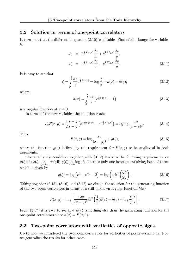
§3 Two-point correlators from the Toda hierarchy
3.2 Solution in terms of one-point correlators
It turns out that the differential equation (3.10) is solvable. First of all, change the variablesto
dη = e12F (x,x)dx
x+ e
12F (y,y)dy
y,
dζ = e12F (x,x)dx
x− e
12F (y,y)dy
y. (3.11)
It is easy to see that
ζ =
x∫
y
dz
ze
12F (z,z) = log
x
y+ h(x) − h(y), (3.12)
where
h(x) =
x∫
0
dz
z
(
e12F (z,z) − 1
)
(3.13)
is a regular function at x = 0.In terms of the new variables the equation reads
∂ηF (x, y) =1
2
x+ y
x− y
(
e−12F (y,y) − e−
12F (x,x)
)
= ∂η logxy
(x− y)2. (3.14)
ThusF (x, y) = log
xy
(x− y)2+ g(ζ), (3.15)
where the function g(ζ) is fixed by the requirement for F (x, y) to be analitycal in botharguments.
The analitycity condition together with (3.12) leads to the following requirements ong(ζ): i) g(ζ) ∼
ζ→±∞±ζ; ii) g(ζ) ∼
ζ→0log ζ2. There is only one function satisfying both of them,
which is given by
g(ζ) = log(
eζ + e−ζ − 2)
= log
(
4sh2
(
ζ
2
))
. (3.16)
Taking together (3.15), (3.16) and (3.12) we obtain the solution for the generating functionof the two-point correlators in terms of a still unknown regular function h(x)
F (x, y) = log
[
4xy
(x− y)2sh2
(
1
2(h(x) − h(y) + log
x
y)
)]
. (3.17)
From (3.17) it is easy to see that h(x) is nothing else than the generating function for theone-point correlators since h(x) = F (x, 0).
3.3 Two-point correlators with vorticities of opposite signs
Up to now we considered the two-point correlators for vorticities of positive sign only. Nowwe generalize the results for other cases.
153

Article I: Correlators in 2D string theory with vortex condensation
First of all, the case of both negative signs can be directly obtained from the previousone. The corresponding equation which is derived from the coefficient in front of y−ny−m inthe Hirota equation looks as (3.1)
[
2pn+m(D−) − pn(D−)D−m − pm(D−)D−n]
τs · τs+1 = 0. (3.18)
The only difference is that τs and τs+1 are exchanged. Due to this there is an additionalminus in the definition of X0,−n. So we should distinguish two types of correlators
X±0,n := ∓i 1
|n|∂2
∂tn∂µF0, n 6= 0, (3.19)
X±n,m := 2 1
|n||m|∂2
∂tn∂tmF0, n,m 6= 0. (3.20)
With this definition, the generating functions of the correlators for positive and negativevorticities are
F±(x, y) =∞∑
n,m=0
xnymX±±n,±m, (3.21)
Despite of this minus all equations for the case of negative vorticities being written in termsof X−
n,m are the same as for the case of positive ones. As a result F−(x, y) is given by the samesolution (3.17) as F+(x, y). The only difference between them is the generating function ofthe one-point correlators h which should be replaced in (3.17) by h± correspondingly.
To find the correlators with vorticities of opposite signs, take the coefficient in the Hirotaequation in front of yny−m and set i = 1. Then we obtain the following equation
−2pn(D+)D−mτs+2 · τs =[
−2pm(D−)Dn + D−1D−mDn
]
τs+1 · τs+1,
pn(D+)D−mτs+2 · τs = pm(D−)Dnτs+1 · τs+1. (3.22)
The last term in the first line vanishes since it always gives rise to Dk(Fs+1 ·1−1 ·Fs+1) = 0.In general, the one-point correlators appearing from τs+k · τs are always supplied with thecoefficient k what follows from (2.20). Due to this in the right hand side there are no one-point correlators whereas in the left hand side they enter with the coefficient 2. This equationis valid also for m = 0 if we take D0 ≡ −2 instead of the previous choice. However, for n = 0it is never fulfilled.
The arguments similar to those of Section 1 lead to the following equation for the gener-ating function
A[
y∂y(G(x, y) − 2h−(y)) − 2]
e12F+(x,x)+h+(x) =
1
y∂xG(x, y)e
12F−(y,y)−h−(y), (3.23)
where we have introduced
A = exp(
−∂2µF0
)
= ξ−Re−∂2wf0, (3.24)
G(x, y) =∞∑
n,m=1xnymXn,−m. (3.25)
Using (3.13) we can rewrite (3.23) as follows
[
A∂x(xeh+(x))
]−1∂x +
[
∂y(1
ye−h
−(y))
]−1
∂y
G(x, y) = −2yeh−(y). (3.26)
154

§4 One-point correlators
It is clear that the solution of this equation looks as
G(x, y) = 2 log(
yeh−(y)
)
+ f(1
ye−h
−(y) − Axeh+(x)). (3.27)
The unknown function f is determined by the analitycity of G(x, y). Requiring cancelationof the logarithmic singularity at y = 0 we obtain that f(z) = 2 log z, As a result we find thegenerating function
G(x, y) = 2 log(
1 − Axyeh+(x)+h−(y)
)
. (3.28)
Let us note that the equations (3.17) and (3.28) resemble the equations for two-pointcorrelators of the two-matrix model found in [17].
4 One-point correlators
4.1 Equation for the generating function
Now we should work out an equation for the one-point correlators. We can always putt1 = −t−1 (corresponding to λ1 = λ−1, see (2.12)). From the equations written below forpositive vorticities it is clear that in this case h±(x) coincide with each other. For this reasonwe omit in the following the inessential sign label in h(x). The case of general t’s can be
obtained from the previous one by the substitution h±(x) = h(
(−t−1/t1)±1/2x
)
. It can be
easily seen from (2.26) and is due to the total vorticity conservation. Accordingly,
F±(x, y) = F(
(−t−1/t1)±1/2x, (−t−1/t1)
±1/2y)
, (4.1)
G(x, y) = Gt1=−t−1
(
(−t−1/t1)1/2x, (−t−1/t1)
−1/2y)
. (4.2)
The equation we are looking for arises from two facts: i) we know the dependence ofthe free energy on t±1 and µ (2.28), (2.29); ii) the system of equations for the correlators istriangular. Due to this we can express X±1,n through X0,n by a linear integral-differentialoperator. Namely, in terms of the generating functions we can write
∂yF+(x, 0) = K(+)h(x) + X+
1,0, (4.3)
∂yG(x, 0) = K(−)h(x), (4.4)
where the operators K(±) are to be found. The last term in the first line is explicitly addedsince in our notations F+(0, 0) = X+
0,0 = 0. Moreover, we can rewrite these equations interms of the generating function for the one-point correlators only. Indeed, from (3.17) and(3.28) we obtain
K(+)h(x) =2
x
(
1 − e−h(x))
− 2X+0,1, (4.5)
K(−)h(x) = −2Axeh(x). (4.6)
155
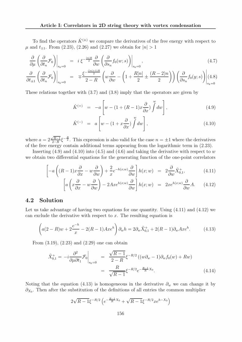
Article I: Correlators in 2D string theory with vortex condensation
To find the operators K(±) we compare the derivatives of the free energy with respect toµ and t±1. From (2.23), (2.26) and (2.27) we obtain for |n| > 1
∂
∂µ
(
∂
∂tnF0
)∣
∣
∣
∣
∣
sk=0
= i ξ−|n|R
2∂
∂w
(
∂
∂snf0(w; s)
)∣
∣
∣
∣
∣
sk=0
, (4.7)
∂
∂t±1
(
∂
∂tnF0
)∣
∣
∣
∣
∣
sk=0
= ∓ξ− (|n|+1)R
2
2 − R
(
w∂
∂w−(
1 +R|n|
2± (R− 2)n
2
))(
∂
∂snf0(y; s)
)
∣
∣
∣
∣
∣
∣
sk=0
.(4.8)
These relations together with (3.7) and (3.8) imply that the operators are given by
K(+) = −a
w − (1 + (R− 1)x∂
∂x)
w∫
dw
, (4.9)
K(−) = a
w − (1 + x∂
∂x)
w∫
dw
, (4.10)
where a = 2√R−1
2−R ξ−R2 . This expression is also valid for the case n = ±1 where the derivatives
of the free energy contain additional terms appearing from the logarithmic term in (2.23).Inserting (4.9) and (4.10) into (4.5) and (4.6) and taking the derivative with respect to w
we obtain two differential equations for the generating function of the one-point correlators
[
−a(
(R − 1)x∂
∂x− w
∂
∂w
)
+2
xe−h(x;w) ∂
∂w
]
h(x;w) = 2∂
∂wX+
0,1, (4.11)
[
a
(
x∂
∂x− w
∂
∂w
)
− 2Axeh(x;w) ∂
∂w
]
h(x;w) = 2xeh(x;w) ∂
∂wA. (4.12)
4.2 Solution
Let us take advantage of having two equations for one quantity. Using (4.11) and (4.12) wecan exclude the derivative with respect to x. The resulting equation is
(
a(2 − R)w + 2e−h
x− 2(R− 1)Axeh
)
∂wh = 2∂wX+0,1 + 2(R− 1)∂wAxe
h. (4.13)
From (3.19), (2.23) and (2.29) one can obtain
X+0,1 = −i ∂2
∂µ∂t1F0
∣
∣
∣
∣
∣
sk=0
=
√R− 1
2 −Rξ−R/2 ((w∂w − 1)∂wf0(w) +Rw)
=R√R− 1
ξ−R/2e−R−1
RX0 . (4.14)
Noting that the equation (4.13) is homogeneous in the derivative ∂w we can change it by∂X0 . Then after the substitution of the definitions of all entries the common multiplier
2√R− 1ξ−R/2
(
e−R−1
RX0 +
√R − 1ξ−R/2xeh−X0
)
156

§4 One-point correlators
can be canceled. As a result we obtain the following simple equation(
1 − ξR/2
x√R − 1
eR−1
RX0e−h
)
∂X0h = 1. (4.15)
This equation can be trivially integrated giving after the proper choice of the integrationconstant
e1Rh − zeh = 1, (4.16)
where z = ξ−R/2√R−1
xe−R−1
RX0 . As it is easy to check this solution satisfies both equations (4.11)
and (4.12).
4.3 One-point correlators of fixed vorticities
Explicit expressions for the one-point correlators are given by the coefficients of the expansionin x by the generating function h(x) satisfying equation (4.16). To find them we can useequation 5.2.13.30 in [18]
1
bsb =
∞∑
n=0
zn
n!
Γ(na + b)
Γ(n(a− 1) + b+ 1), (4.17)
s = 1 + zsa. (4.18)
Taking s = e1Rh, a = R we obtain for b = kR
ekh = kR∞∑
n=0
zn
n!
Γ((n+ k)R)
Γ((n+ k)R − n + 1). (4.19)
Also the limit b→ 0 gives
h = R∞∑
n=1
zn
n!
Γ(nR)
Γ(n(R− 1) + 1). (4.20)
This means that the derivative with respect to µ of the one-point correlator is
∂2
∂µ∂tnF0 =
iΓ(nR + 1)
n!Γ(n(R − 1) + 1)
ξ−nR/2
(R− 1)n/2e−n
R−1R
X0. (4.21)
After integration over µ and taking into account the relation (2.12) we obtain the followingone-point correlators of operators of vorticity n in the spherical limit
Kn =1
2 sinπnR
Γ(nR + 1)
n!Γ(n(R − 1) + 1)
ξ−nR+2
2
(R− 1)n/2
e−n(R−1)+1
RX0
n(R − 1) + 1− e−(n+1) R−1
RX0
n+ 1
. (4.22)
(Here the lower limit of the integration is chosen to beX0 = +∞. Only this choice reproduces∂λ1F0 from (2.29).) In particular, in the limit µ→ 0 (X0 → 0) corresponding to string theoryon the black hole background (in fact, only the point R = 3/2 is supposed to describe theconventional black hole) we find
Kn =1
2 sin πnR
ξ−nR+2
2
(R− 1)n/2(2 − R)nΓ(nR + 1)
(n+ 1)!Γ(n(R− 1) + 2). (4.23)
157

Article I: Correlators in 2D string theory with vortex condensation
5 Results for two-point correlators
5.1 Correlators with vorticities of opposite signs
These correlators are given by the expansion coefficients of the generating function (3.28).This function can be easily expanded in eh for which the series (4.19) can be used. Thisleads to the following expansion
G(x, y) = −2∞∑
k=1
Bk
kzk(x)zk(y)
∞∑
n=0
∞∑
m=0
CknC
kmz
n(x)zm(y)
= −2∞∑
n,m=1
zn(x)zm(y)min(n,m)∑
k=1
Bk
kCkn−kC
km−k, (5.1)
where
B = A(R− 1)ξRe2R−1
RX0 = (R− 1)e
R−2R
X0 , (5.2)
Ckn =
kR
n!
Γ((n + k)R)
Γ(n(R− 1) + kR + 1). (5.3)
The two-point correlators appear to be
Kn,−m = −Γ(nR + 1)
2 sin πnR
Γ(mR + 1)
2 sin πmR
ξ−(n+m)R/2
(R− 1)(n+m)/2e−(n+m) R−1
RX0 ×
×min(n,m)∑
k=1
k(R− 1)kekR−2
RX0
(n− k)!(m− k)!Γ(n(R− 1) + k + 1)Γ(m(R− 1) + k + 1). (5.4)
To get the result in the black hole limit it is enough to set X0 = 0 in the above expression.It is worth to give also the result for the ratios of correlators which do not depend on
possible leg-factors — wave function renormalisations of the operators (see for ex. [12]):
Kn,−mKnK−m
= − ξ2
(2 − R)2nm
min(n,m)∑
k=1
k(R − 1)k(n+ 1)!(m+ 1)!Γ(n(R− 1) + 2)Γ(m(R− 1) + 2)
(n− k)!(m− k)!Γ(n(R− 1) + k + 1)Γ(m(R− 1) + k + 1).
(5.5)Since they can in principle be compared with CFT calculations in the black hole limit werestrict ourselves only to this particular case.
5.2 Correlators with vorticities of same signs
To investigate this case we should expand (3.17) in x and y. The expansion in the firstargument gives for n > 0
∂nxF (0, y) =2
yn
(
1
n−
n∑
k=1
2
kzn−k(y)e−kh(y)Ck
n−k
)
− X0,n
= −2ξ−nR/2
(R− 1)n/2e−n
R−1R
X0
∞∑
m=0
zm(y)n∑
k=1
1
kCkn−kC
−km+k − X0,n
+2
yn
(
1
n−
n∑
m=1
zn−m(y)n∑
k=m
1
kCkn−kC
−kk−m
)
. (5.6)
158
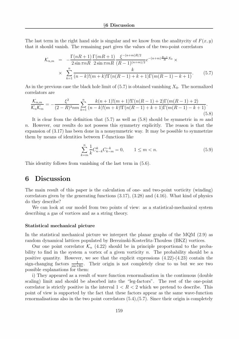
§6 Discussion
The last term in the right hand side is singular and we know from the analitycity of F (x, y)that it should vanish. The remaining part gives the values of the two-point correlators
Kn,m = −Γ(nR + 1)
2 sinπnR
Γ(mR + 1)
2 sinπmR
ξ−(n+m)R/2
(R− 1)(n+m)/2e−(n+m) R−1
RX0 ×
×n∑
k=1
k
(n− k)!(m+ k)!Γ(n(R − 1) + k + 1)Γ(m(R− 1) − k + 1). (5.7)
As in the previous case the black hole limit of (5.7) is obtained vanishing X0. The normalizedcorrelators are
Kn,m
KnKm= − ξ2
(2 −R)2nm
n∑
k=1
k(n + 1)!(m+ 1)!Γ(n(R− 1) + 2)Γ(m(R− 1) + 2)
(n− k)!(m + k)!Γ(n(R− 1) + k + 1)Γ(m(R− 1) − k + 1).
(5.8)It is clear from the definition that (5.7) as well as (5.8) should be symmetric in m and
n. However, our results do not possess this symmetry explicitly. The reason is that theexpansion of (3.17) has been done in a nonsymmetric way. It may be possible to symmetrizethem by means of identities between Γ-functions like
n∑
k=m
1
kCkn−kC
−kk−m = 0, 1 ≤ m < n. (5.9)
This identity follows from vanishing of the last term in (5.6).
6 Discussion
The main result of this paper is the calculation of one- and two-point vorticity (winding)correlators given by the generating functions (3.17), (3.28) and (4.16). What kind of physicsdo they describe?
We can look at our model from two points of view: as a statistical-mechanical systemdescribing a gas of vortices and as a string theory.
Statistical mechanical picture
In the statistical mechanical picture we interpret the planar graphs of the MQM (2.9) asrandom dynamical lattices populated by Berezinski-Kosterlitz-Thouless (BKZ) vortices.
Our one point correlator Kn (4.22) should be in principle proportional to the proba-bility to find in the system a vortex of a given vorticity n. The probability should be apositive quantity. However, we see that the explicit expressions (4.22)-(4.23) contain thesign-changing factors 1
sinπRn. Their origin is not completely clear to us but we see two
possible explanations for them:i) They appeared as a result of wave function renormalisation in the continuous (double
scaling) limit and should be absorbed into the “leg-factors”. The rest of the one-pointcorrelator is strictly positive in the interval 1 < R < 2 which we pretend to describe. Thispoint of view is supported by the fact that these factors appear as the same wave-functionrenormalisations also in the two point correlators (5.4),(5.7). Since their origin is completely
159

Article I: Correlators in 2D string theory with vortex condensation
due to the change of variables (2.12) these factors appear to be a general feature for allmultipoint correlators.
ii) The sign-changing might be a consequence of the fact that our approach based on theHirota equations (describing directly the double scaling limit) does not keep track of non-universal terms due to the ultraviolet (lattice) cut-off in the system. Such UV divergencesare well known in the Coulomb gas description of the BKT system: they usually correspondto the proper energy of a vortex. In that case the correlators we calculated above are only theuniversal parts of the full correlators containing also big positive non-universal contributions.These universal parts cannot be interpreted as full probabilities and have no reason to bepositively defined.
To prove or reject these explanations we have to see what happens with the individualvortices in the process of taking the double scaling limit, from planar graphs picture to theinverted oscillator description. It is not an easy, although not hopeless, task which we leavefor the future.
String theory picture
The MQM describes also the two-dimensional bosonic string theory in compact imaginarytime (i.e. at finite temperature). Due to the FZZ [5] conjecture, at the vanishing cosmo-logical constant it can be also interpreted as a string theory in the Euclidean 2D black holebackground (at least at R = 3/2) [3]. Our one-point correlators should contain informationabout the amplitudes of emission of winding modes by the black hole, whereas the two-pointcorrelators describe the S-matrix of scattering of the winding states from the tip of the cigar(or from the Sine-Liouville wall). However, the exact correspondence is lacking due to theabsence of the proper normalization of the operators. In [5] and [6] some two- and three-pointcorrelators were computed in the CFT approach to this theory. It would be interesting tocompare their results with the correlators calculated in this paper from the MQM approach.However there are immediate obstacles to this comparison.
First of all, these authors do not give any results for the one point functions of vortices.In the conformal theory such functions are normally zero since the vortex operators have thedimension one. But in the string theory we calculate the averages of a type
⟨
∫
d2σ Vn(σ)⟩
integrated over the parameterization space. They are already quantities of zero dimension,and the formal integration leads to the ambiguity 0 ∗ ∞ which should in general give afinite result. Another possible reason for vanishing of the one-point correlator could be theadditional infinite W-symmetry found in [7] for the CFT (2.7) (at R = 3/2, µ′ = 0).2 Thegenerators of this symmetry do not commute with the vortex operators Vn, n 6= ±1. Henceits vacuum average should be zero, unless there is a singlet component under this symmetryin it. Our results suggest the presence of such a singlet component.
Note that the one-point functions were calculated [6] in a non-conformal field theory withthe Lagrangian:
L =1
4π
[
(∂X)2 + (∂φ)2 − 2Rφ+m(
e−12φ + e
12φ)
cos(3
2X)]
. (6.1)
2We thank A.Zamolodchikov for this comment
160

§6 Discussion
This theory coincides with the CFT (2.7) (again at R = 3/2 and µ′ = 0) in the limit
m → 0, φ0 → −∞, with λ = me−12φ0 fixed, where φ0 is a shift of the zero mode of the
Liouville field φ(z). So we can try to perform this limit in the calculated one-point functionsdirectly. As a result we obtain K(m)
n ∼ m2λ3n−4. The coefficient we omitted is given by acomplicated integral which we cannot perform explicitly. It is important that it does notdepend on the couplings and is purely numerical. We see that, remarkably, the vanishingmass parameter enters in a constant power which is tempting to associate with the measured2σ of integration. Moreover, the scaling in λ is the same as in (4.23) (at R = 3/2) up tothe n-independent factor λ−8. All these n-independent factors disappear if we consider thecorrelators normalized with respect to K(m)
1 which is definitely nonzero. They behave like∼ λ3(n−1) what coincides with the MQM result.
The two point correlators for the CFT (2.7) with µ′ = 0 are calculated in [6] only inthe case of vortex operators of opposite and equal by modulo vorticities. They should be inprinciple compared to our Kn,−n correlators from (5.4). However, we should compare onlyproperly normalized quantities, knowing that the matrix model correlators generally differfrom the CFT correlators by the leg-factors. To fix the normalization we have to comparethe quantities similar to (5.5) and (5.8) which are not available in the CFT approach.
A lot of interesting physical information is contained in multipoint correlators (3-pointand more) which we did not consider in this paper and some of which are calculated inthe CFT approach of [5, 19]. The direct calculations from the Hirota equations look verytedious. Hopefully the collective field theory approach of [20] can help on this way.
A lot is to be done to learn how to extract information about the black hole physicsfrom the correlators. First of all, we have only calculated some vortex (winding modes)correlators in our MQM approach. The vertex (momentum modes, or tachyon) correlatorsare unavailable in the Toda hierarchy approach used here and do not seem to fit any knownintegrable structure in the MQM, although they are in principle calculable directly from theMQM in the large N limit. On the other hand, they bear even a more important informationabout the system than the winding correlators: they describe the S-matrix of scattering oftachyons off the black hole and can be used to “see” the black hole background explicitly.The one-point tachyon correlators may give information about the black hole radiation. Ingeneral, the MQM approach seems to be a good chance to work out a truly microscopicpicture for the 2D black hole physics.
Acknowledgments
We would like to thank V. Fateev, I. Kostov, D. Kutasov and A. and Al. Zamolodchikovfor interesting discussions. This research of S.A. was supported in part by European net-work EUROGRID HPRN-CT-1999-00161. The research of V.K. was supported in part byEuropean Contract HPRN-CT-2000-00122.
161

Article I: Correlators in 2D string theory with vortex condensation
Appendix A.
Let us investigate which terms will survive in the dispersionless limit in the equation (3.1).This limit corresponds to ξ −→ 0. It is clear that all terms have the form
l∏
j=1
Dkj
τs+1 · τs (A.1)
with n =l∑
j=1kj fixed. When we rewrite them in terms of the free energy Fs = log τs we
obtain a set of terms of a kind
eFs+Fs+1
p∏
j=1
([ qj∏
i=1
∂
∂tkji
]
(Fs+1 + (−1)qjFs)
)
, (A.2)
wherep∑
j=1qj = l. In the dispersionless limit (2.22), (2.27) and (2.20) imply
Fs+1 + Fs ∼ 2F0, (A.3)
Fs+1 − Fs ∼ −iξ ∂∂w
F0, (A.4)
The main contribution in the dispersionless limit comes from the terms with the minimaldegree of ξ. The total degree of ξ for a given term is
l∑
j=1
∆[tkj] − 2p+ r = l − 2p+ r − nR
2, (A.5)
where r is the number of odd qj. It is easy to see that the minimum is achieved when allqj = 1 or 2 and it equals −nR
2what is independent on all particular parameters and hence
is similar for all terms in the equation. It means that only two- and one-point correlatorssurvive.
Appendix B.
Combine together all terms with Dk and separately with Xk in the exponents of the eq.(3.5). Then due to vanishing of D2Xk we can apply the formula eA+B = eAeBe−
12[A,B] which
is valid for operators having c-number commutator. This gives
2x−y
xe
∞∑
k=1
xkXk
e
12
∞∑
k,l=1
xk+lXk,l
− ye
∞∑
k=1
ykXk
e
12
∞∑
k,l=1
yk+lXk,l
= (B.1)
(
1 +∞∑
m=1ym(Dm +Xm)
)
e
∞∑
k=1
xkXk
e
12
∞∑
k,l=1
xk+lXk,l
+(
1 +∞∑
n=1xn(Dn +Xn)
)
e
∞∑
k=1
ykXk
e
12
∞∑
k,l=1
yk+lXk,l
162

References
The right hand side of this equation can be rewritten as follows
(
1 +∞∑
m=1mym
(
Xm +∞∑
n=1xnXn,m
))
e
∞∑
n=1
xnXn+ 12
∞∑
k,l=1
xk+lXk,l
+
(
1 +∞∑
n=1nxn
(
Xn +∞∑
m=1ymXn,m
))
e
∞∑
m=1
ymXm+ 12
∞∑
k,l=1
yk+lXk,l
. (B.2)
Due to (3.7) we obtain
x+yx−y
e
12
∞∑
k,l=0
xk+lXk,l
− e
12
∞∑
k,l=0
yk+lXk,l
=
(
∞∑
n,m=0mxnymXn,m
)
e
12
∞∑
k,l=0
xk+lXk,l
+
(
∞∑
n,m=0nxnymXn,m
)
e
12
∞∑
k,l=0
yk+lXk,l
= 0, (B.3)
what can be written in terms of the generating function (3.9) as in (3.10).
References
[1] D. Gross and I. Klebanov, Nucl. Phys. B344 (1990) 475.
[2] D. Boulatov and V.Kazakov, preprint LPTENS 91/24 (1991), Int. J. Mod. Phys. A8(1993) 809, revised version: hep-th/0012228.
[3] V. Kazakov, I. Kostov and D. Kutasov, Matrix Model for the Two Dimensional BlackHole, hep-th/0101011.
[4] J. Hoppe, V. Kazakov and I. Kostov, Nucl. Phys. B571 (2000) 479.
[5] V. Fateev, A. Zamolodchikov and Al. Zamolodchikov, unpublished.
[6] P. Baseilhac and V. Fateev, Nucl. Phys. B532 (1998) 567.
[7] V. Fateev, Phys. Lett. B359 (1995) 397.
[8] E. Witten, Phys. Rev. D 44 (1991) 314.
[9] R. Dijkgraaf, E. Verlinde and H. Verlinde, Nucl. Phys. B 371 (1992) 269.
[10] D. Gross and I. Klebanov, Nucl. Phys. B354 (1990) 459.
[11] G. Moore, Gravitational Phase Transitions and the Sine-Gordon Model, hep-th/9203061.
[12] I. Klebanov, String Theory in Two Dimensions, Lectures at the ICTP Spring School onString Theory and Quantum Gravity, Trieste (1991), hep-th/9108019.
163

Article I: Correlators in 2D string theory with vortex condensation
[13] E. Brezin, V.A. Kazakov and Al.B. Zamolodchikov, Nucl. Phys. B338 (1990) 673; D.Gross and N. Miljkovic, Phys. Lett. B 238 (1990) 217; P. Ginsparg and J. Zinn-Justin,Phys. Lett. B 240 (1990) 333; J. Parisi, Phys. Lett. B 238 (1990) 209.
[14] R. Hirota, Direct Method in Soliton Theory, Solitons, Ed. by R. K. Bullogh and R. J.Caudrey, Springer, 1980.
[15] K. Ueno and K. Takasaki, Adv. Stud. Pure Math. 4 (1984) 1; K. Takasaki, Adv. Stud.Pure Math. 4 (1984) 139.
[16] M. Jimbo and T. Miwa, Publ. RIMS, Kyoto Univ. 19, No. 3 (1983) 943.
[17] J.-M. Daul, V.A. Kazakov and I.K. Kostov, Nucl. Phys. B 409 (1993) 311, hep-th/9303093.
[18] A. Prudnikov, Yu. Brichkov, and O. Marychev, ”Integrals and Series”, Nauka, Moscow,1981.
[19] J. Teschner, Nucl. Phys. B 546 (1999) 390, hep-th/9712256; Nucl. Phys. B 546 (1999)369, hep-th/9712258; Nucl. Phys. B 571 (2000) 555, hep-th/9906215.
[20] I.K. Kostov, the work in progress.
164
Article II
Time-dependent backgrounds of
2D string theory
Nucl. Phys. B640 (2002) 119


LPTENS-02/33, SPHT-T02/055hep-th/0205079
Time-dependent backgrounds of 2D stringtheory
Sergei Yu. Alexandrov,123 Vladimir A. Kazakov1, and Ivan K. Kostov2
1Laboratoire de Physique Theorique de l’Ecole Normale Superieure,†
24 rue Lhomond, 75231 Paris CEDEX, France2Service de Physique Theorique, CNRS - URA 2306, C.E.A. - Saclay,
F-91191 Gif-Sur-Yvette CEDEX, France3V.A. Fock Department of Theoretical Physics, St. Petersburg University, Russia
We study possible backgrounds of 2D string theory using its equivalence with a systemof fermions in upside-down harmonic potential. Each background corresponds to a certainprofile of the Fermi sea, which can be considered as a deformation of the hyperbolic profilecharacterizing the linear dilaton background. Such a perturbation is generated by a set ofcommuting flows, which form a Toda Lattice integrable structure. The flows are associatedwith all possible left and right moving tachyon states, which in the compactified theory havediscrete spectrum. The simplest nontrivial background describes the Sine-Liouville stringtheory. Our methods can be also applied to the study of 2D droplets of electrons in a strongmagnetic field.
†Unite de Recherche du Centre National de la Recherche Scientifique et de l’Ecole Normale Superieureet a l’Universite de Paris-Sud.

Article II: Time-dependent backgrounds of 2D string theory
1 Introduction
One of the most important problems of the modern string theory is a search for new nontrivialbackgrounds and the study of the underlying string dynamics. In most of the cases thetarget space metric of such backgrounds is curved and often it incorporates the black holesingularities. In the superstring theories, the supersymmetry allows for some interestingnontrivial solutions which are stable and exact. But the string theory on such backgroundsis usually an extremely complicated sigma-model, very difficult even to formulate it explicitly,not to mention studying quantitatively its dynamics.
The two-dimensional bosonic string theory is a rare case of sigma-model where such adynamics is integrable, at least for some particular backgrounds, including the dilatonicblack hole background. A physically transparent way to study the perturbative (one loop)string theory around such a background is provided by the CFT approach. However, oncewe want to achieve more ambitious quantitative goals, especially in analyzing higher loopsor multipoint correlators, we have to address ourselves to the matrix model approach to the2D string theory proposed in [1] in the form of the matrix quantum mechanics (MQM) of [2].The string theory has been constructed as the collective field theory (the Das-Jevicki-Sakitatheory), in which the only excitation, the massless ”tachyon”, was related to the eigenvaluedensity of the matrix field.
In the framework of MQM it is difficult to formulate directly a string theory in a nontrivialbackground metric since the operators perturbing the metric do not have a simple realization.However, we can perturb the theory by other operators, like tachyon or winding operators.We hope that such a perturbation can also produce a curved metric but in an indirect way.An example of such a duality was given in [3] where the 2D black hole background is inducedby a winding mode perturbation.
The 2D string theory in the simplest, translational invariant background (the lineardilaton background) is described by the singlet sector of MQM with inversed quadraticpotential. In the singlet sector of the Hilbert space, the eigenvalues have Fermi statistics,and the problem of calculating the S-matrix of the string theory tachyon becomes a ratherstandard problem in a quantum theory of a one-dimensional nonrelativistic free fermionicfield. The tree-level S-matrix can be extracted by considering the propagation of ”pulses”along the Fermi surface and their reflection off the ”Liouville wall” [4, 5].
The very existence of a formulation in terms of free fermions indicates that the 2D stringtheory should be integrable. For example, the fermionic picture allows to calculate the exactS-matrix elements. Each S-matrix element can be associated with a single fermionic loopwith a number of external lines [6]. One can then expect that the theory is also solvable ina nontrivial, time-dependent background generated by a finite tachyonic source. Dijkgraaf,Moore and Plesser [7] demonstrated that this is indeed the case when the allowed momentaform a lattice as in the case of the compactified Euclidean theory. In [7] it has been shownthat the string theory compactified at any radius R possesses the integrable structure of theToda lattice hierarchy. However, this important observation had not been, until recently,really exploited. The Toda structure is too general, and it becomes really of use only ifaccompanied by an initial condition or a constraint (a ”string equation”), which eliminatesall the solutions but one. Thus the first results for a nontrivial background in case of ageneral radius were obtained as a perturbative expansion in the tachyon source [8].
168
§1 Introduction
Recently, the Toda integrable structure of the compactified Euclidean 2D string theorywas rediscovered [9, 10] and used to find the explicit solution of the theory [10, 11]. Finally,the string equation at an arbitrary compactification radius was found in [12]. These papersstudied the T-dual formulation of the string theory, where instead of the discrete spectrumof tachyon excitations the winding modes of the string around the compactification circle(Berezinski-Kosterlitz-Thouless vortices) were used. These modes appear in the non-singletsectors of MQM [13] and can be generated by imposing twisted periodic boundary conditions[14].
In this paper we return to the study of the Toda integrable structure of tachyon excita-tions of 2D string theory originated in [7]. It describes special perturbations of the groundstate within the singlet sector of the MQM. We will construct the Lax operators as operatorsin the Hilbert space of the singlet sector of MQM. We will be able to find an interpretationof the Toda spectral parameters in terms of the coordinates of the two-dimensional targetphase space and interpret the solutions of the Toda hierarchy in terms of the shape of theFermi sea. In particular, we find the explicit shape of the Fermi sea for the Sine-Liouvillestring theory.
We can give two different interpretations of our problem. The first one is that of a2D string theory in Minkowski space in a non-stationary background. The simplest, time-independent ground state of the theory is characterized by a condensation of the constanttachyon mode, which is controlled by the cosmological constant µ. Here we will studymore general, time-dependent backgrounds characterized by a set of coupling constants t±nassociated with non-trivial tachyon modes with purely imaginary energies En = in/R, whereR is a real number. Since the incoming/outgoing tachyons with imaginary energies have wavefunctions exponentially decreasing/increasing with time, such a ground state will containonly incoming tachyons in the far past and only outgoing tachyons in the far future. In otherwords, the right and left vacua are replaced by coherent states depending correspondinglyon the couplings tn and t−n (n = 1, 2, ...), which will be identified with the “times” of theToda hierarchy. The coherent states of bosons modify the asymptotics of the profile of theFermi sea at far past and future, without changing the number of fermions. The flow of thefermionic liquid is no more stationary, but its time dependence happens to be quite trivial,and the profiles of the Fermi sea at different moments of time are related by Lorentz boosts.
The second interpretation of our analysis is that we consider perturbations of an Eu-clidean 2D string theory in which the Euclidean time is compactified at some length β = 2πR.Together with the cosmological term, we allow all possible vertex operators with momentan/R, n ∈ Z. The simplest case of such a perturbation is the Sine-Liouville theory. This casewill be considered in detail and the shape of the Fermi sea produced by the Sine-Liouvilleperturbation will be found explicitly. The solution we have found exhibits interesting ther-modynamical properties, which may be relevant to the thermodynamics of the string theoryon the dilatonic 2D black hole background.
Let us mention also another possible application of our analysis: the fermionic systemthat appears in MQM is similar to the problem of two-dimensional fermions in a strongtransverse magnetic field [15]. The electrons filling the first Landau level form stationarydroplets of Fermi liquid, similar to that of the eigenvalues in the phase space of MQM. Theform of such droplets is also described by the Toda hierarchy [16]. Our problem might berelated to the situation in which two such droplets are about to touch, which can happen at
169

Article II: Time-dependent backgrounds of 2D string theory
a saddle point of the effective potential [17].The paper is organized as follows. In section 2 we will remind the CFT formulation of
the 2D string theory. In section 3 the MQM in the inverted harmonic potential in the “light-cone” phase space variables is formulated and the free fermion structure of its singlet sectoris revealed. In section 4 the one particle wave functions are studied. In section 5, after thedescription of the fermionic ground state, tachyonic perturbations are introduced and theequations defining the corresponding time-dependent profile of the Fermi sea are derived.In section 6 the Toda integrable structure of the perturbations restricted to a lattice ofEuclidean momenta is derived directly from the Schroedinger picture for the free fermions.In section 7 we recover the solution of the Sine-Liouville model and describe explicitly itsFermi sea profile. In section 8 we reproduce the free energy of the perturbed system fromthe profile of the Fermi sea. The section 9 is devoted to conclusions and in section 10 wediscuss some problems and future perspectives. In particular, we propose a 3-matrix modeldescribing the 2D string theory perturbed by both tachyon and winding modes. In theappendix the one particle wave functions of the type II model, defined on both sides of thequadratic potential, in the “light cone” formalism are presented.
2 Tachyon and winding modes in 2D Euclidean string
theory
The 2D string theory is defined by Polyakov Euclidean string action
S(X, g) =1
4π
∫
d2σ√
detg[gab∂aX∂bX + µ], (2.1)
where the bosonic field X(σ) describes the embedding of the string into the Euclidean timedimension and gab is a world sheet metric. In the conformal gauge gab = eφ(σ)gab, where gab
is a background metric, the dilaton field φ becomes dynamical due to the conformal anomalyand the world-sheet CFT action takes the familiar Liouville form
S0 =1
4π
∫
world sheetd2σ [(∂X)2 + (∂φ)2 − 2Rφ+ µe−2φ + ghosts]. (2.2)
This action describes the unperturbed linear dilaton string background corresponding to theflat 2D target space (X, φ).
In the target space this theory possesses only one propagating degree of freedom whichcorresponds to tachyon field. If the Euclidean time is compactified to a circle of radius R,X(σ) ≡ X(σ)+2πR, the spectrum of admissible momenta is discrete: pn = n/R, n ∈ Z. Inthis case there is also a discrete spectrum of vortex operators, describing the winding modes(Kosterlitz-Thouless vortices) on the world sheet. A vortex of charge qm = mR correspondsto a discontinuity 2πmR of the time variable around a point on the world sheet.1 The explicitexpressions of the vertex operators Vp and the vortex operators Vq in terms of the positionfield X = XR +XL and its dual X = XR −XL are
Vp =Γ(|p|)
Γ(−|p|)∫
d2σ eipXe(|p|−2)φ, (2.3)
1At rational values of R there exist additional physical operators (similar to discrete states at the self-dualradius R = 1) containing the derivatives of fields X(σ) and φ(σ), which we will ignore in this paper.
170

§3 MQM in light cone formulation
Vq =Γ(|q|)
Γ(−|q|)∫
d2σ eiqXe(|q|−2)φ. (2.4)
Any background of the compactified 2D string theory can be obtained (at least in the caseof irrational R) by a perturbation of the action (2.2) with both vertex and vortex operators
S = S0 +∑
n6=0
(tnVn + tnVn). (2.5)
Such a theory possesses the T-duality symmetry of the non-perturbed theory X ↔ X,R → 1/R, µ → Rµ [18] if one also exchanges the couplings as tn ↔ tn. Another generalfeature of the theory (2.5) is the existence of the physical scaling of various couplings,including the string coupling gs, with respect to the cosmological coupling µ. It can befound from the zero mode shift of the dilaton φ→ φ+ φ0. In this way we obtain
tn ∼ µ1− 12|n|/R, tn ∼ µ1− 1
2R|n|, gs ∼ µ−1. (2.6)
The scaling (2.6) allows to conclude that at the compactification radius lower than theBerezinski-Kosterlitz-Thouless radius RKT = 1/2 all vertex operators are irrelevant. In theinterval 1/2 < R < 1 the only relevant momenta are p = ±1/R. The theory perturbedby such operators looks as the Sine-Gordon theory coupled to 2d gravity (“Sine-Liouville”theory):
SSG =1
4π
∫
d2σ [(∂X)2 + (∂φ)2 − 2Rφ+ µe−2φ + λe(1R−2)φ cos(X/R)]. (2.7)
It was conjectured by [3] that at R = 2/3 and µ = 0 the “Sine-Liouville” is dual to the[
SL(2,C)SU(2)×U(1)
]
kcoset model with central charge c = 3k
k−2− 1 = 26, which describes the 2D
string theory in the black hole (“cigar”) background.If we go to the Minkowski space, the perturbation (2.5) is made by tachyons with purely
imaginary momenta. In this case there are more general perturbations, generated by tachyonswith any real energies. In the next section we will introduce the matrix formulation of thestring theory in Minkowski space using light-cone coordinates.
3 MQM in light cone formulation
The 2D string theory in Minkowski time appears as the collective field theory for the large-Nlimit of MQM in the inverted oscillator potential [1, 19, 20, 21, 22]. The matrix Hamiltonianis
H =1
2Tr (P 2 −M2), (3.1)
where P = −i∂/∂M and Mij is an N × N hermitian matrix variable. The cosmologicalconstant µ in (2.2) is introduced as a “chemical potential” coupled to the size of the matrixN ,which should be considered as a dynamical variable. In this formulation the time coordinateof the string target space coincides with the MQM time (or its Euclidean analogue X = itin the compactified version of the MQM) and that of the Liouville field is related to thespectral variable of the random matrix.
171

Article II: Time-dependent backgrounds of 2D string theory
The tachyon modes of the string theory are represented by the asymptotic states of thecollective theory. The scattering operators with real energy E and describing right- andleft-moving waves, respectively, are given by [5]
TE− = e−iEt Tr (M + P )iE, TE+ = e−iEt Tr (M − P )−iE. (3.2)
These operators can be used to construct the in- and out-states of scattering theory. Namely,for an in-state, one needs a left-moving wave while the out-state is necessarily given by aright-moving one. The vertex operators (2.3) are tachyons with purely imaginary energiesand are therefore represented by the following chiral operators in the MQM
Vp →
e−pt Tr (M + P )|p|, p > 0,e−pt Tr (M − P )|p|, p < 0.
(3.3)
Since we are interested in perturbations with the chiral operators (3.3), it is natural toperform a canonical transformation to light-cone variables
X± =M ± P√
2(3.4)
and write the matrix Hamiltonian as
H0 = −1
2Tr (X+X− +X−X+), (3.5)
where the matrix operators X± obey the canonical commutation relation
[(X+)ij, (X−)kl ] = −i δilδkj . (3.6)
Define the right and left Hilbert spaces as the spaces of functions of X+ and X− only, withthe scalar product
〈Φ±|Φ′±〉 =
∫
dN2
X± Φ±(X±)Φ′±(X±). (3.7)
The operator of coordinate in the right Hilbert space is the momentum operator in theleft one and the wave functions in the X+ and X− representations are related by a Fouriertransform. The second-order Schrodinger equation associated with the Hamiltonian (3.1)becomes a first-order one when written in the ±-representations
∂tΦ±(X±, t) = ∓Tr
(
X±∂
∂X±+N
2
)
Φ±(X±, t), (3.8)
whose general solution isΦ±(X±, t) = e∓
12N2tΦ
(0)± (e∓tX±). (3.9)
The Hilbert space decomposes into a direct sum of eigenspaces labeled by the irreduciblerepresentations of SU(N), which are invariant under the action of the Hamiltonian (3.5).
The functions ~Φ(r)± = Φ(r,J)
± dim(r)J=1 belonging to given irreducible representation r transform
asΦ
(r,I)± (Ω†X±Ω) =
∑
J
D(r)IJ (Ω)Φ
(r,J)± (X±), (3.10)
172
§4 Eigenfunctions and fermionic scattering
where D(r)IJ is the group matrix element in representation r and I, J are the representation
indices. The wave functions transforming according to given irreducible representation de-pend only on the N eigenvalues x±,1 , . . . , x±,N
and the Hamiltonian (3.5) reduces to its radialpart
H0 = ∓i∑
k
(x±,k∂x±,k
+N
2). (3.11)
A potential advantage of the light-cone approach is that the Hamiltonian (3.11) does notcontain any angular part, which is not the case for the standard one (3.1), whose angularterm induces a Calogero-like interaction.
In the scalar product (3.7), the angular part can also be integrated out, leaving only thetrace over the representation indices:
〈~Φ(r)± |~Φ′(r)
± 〉 =∑
J
∫
∏
k
dx±,k∆2(x±)Φ
(r,J)± (x±)Φ
′(r,J)± (x±), (3.12)
where ∆(x±) is the Vandermonde determinant. If we define
~Ψ(r)± (x±) = ∆(x±)~Φ
(r)± (x±), (3.13)
these determinants disappear from the scalar product. The Hamiltonian for the new func-tions ~Ψ
(r)± (x±) takes the same form as (3.11) but with a different constant term:
H0 = ∓i∑
k
(x±,k∂x±,k
+ 1/2). (3.14)
In the singlet representation, the wave function Ψ±(x±) ≡ Ψ(singlet)± (x±) is a completely
antisymmetric scalar function. The scalar product in the singlet representation is given by
〈Ψ±|Ψ′±〉 =
∫
∏
k
dx±,kΨ±(x±)Ψ′
±(x±). (3.15)
Thus the singlet sector describes a system of N free fermions. The singlet eigenfunctions ofthe Hamiltonian (3.14) are represented by Slater determinants of one-particle eigenfunctionsdiscussed in the next section.
It is known [13, 14, 10] that unlike singlet, which is free of vortices, the adjoint rep-resentation contains string states with a vortex-antivortex pair, and higher representationscontain higher number of such pairs. In what follows we will concentrate on the fermionicsystem describing the singlet sector of the matrix model. We will start from the propertiesof the ground state of the model, representing the unperturbed 2D string background andthen go over to the perturbed fermionic states describing the (time-dependent) backgroundscharacterized by nonzero expectation values of some vertex operators.
4 Eigenfunctions and fermionic scattering
To study the system of non-interacting fermions we have to start with one-particle eigen-functions. The one-particle Hamiltonian in the light-cone variables of the previous sectioncan be written as
H0 = −1
2(x+x− + x− x+), (4.1)
173

Article II: Time-dependent backgrounds of 2D string theory
where x± turn out to be canonically conjugated variables
[x+, x− ] = −i. (4.2)
We can work either in x+ or in x− representation, where the theory is defined in terms offermionic fields ψ±(x±) respectively. General solutions of the Schrodinger equation with theHamiltonian (4.1) written in these representations take the form
ψ±(x±, t) = x−1/2± f±(e∓tx±). (4.3)
There are two versions of the theory, referred in [6] as theories of type I and II. In thetheory of type I the eigenvalues λk of the original matrix field M are restricted to the positivehalf-line. The theory of type II is defined on the whole real axis λ. Such a string theorysplits, at the perturbative level, into two disconnected string theories of type I. Here we willconsider the fermion eigenfunctions in the theory of type I. The theory of type II will beconsidered in Appendix A.
In the light cone formalism it is natural to replace the restriction λ > 0 with x± > 0,which again does not affect the perturbative behavior. In this case the solutions with a givenenergy are ψE
± (x±, t) = e−iEtψE±(x±) with
ψE
± (x±) =1√2πx±iE− 1
2± . (4.4)
The functions (4.4) with E real form two complete systems of δ-function normalized or-thonormal states
〈ψE± |ψE′
± 〉 ≡ ∫∞0 dx± ψE
±(x±)ψE′± (x±) = δ(E − E ′), (4.5)
∫∞−∞ dE ψE
±(x±)ψE± (x′±) = δ(x± − x′±). (4.6)
As any two representations of a quantum mechanical system, the x+ and x− represen-
tations are related by a unitary operator S, which in our case is nothing but the Fouriertransformation on the half-line. The latter is defined by the integral
[Sψ+ ](x−) =∫ ∞
0dx+ K(x− , x+)ψ+(x+), (4.7)
where there are two choices for the kernel:
K(x− , x+) =
√
2
πcos(x−x+) or K(x− , x+) = i
√
2
πsin(x−x+). (4.8)
The sine and the cosine kernels describe two possible theories, which differ only on the non-perturbative level.2 Let us choose the cosine kernel in (4.8) and evaluate the action of the
2The fact that there are two choices for the kernel can be explained as follows. In order to define thetheory of type I for the original second-order Hamiltonian (3.1), we should fix the boundary condition atλ = 0, and there are two linearly independent boundary conditions.
174

§5 String theory backgrounds as profiles of Fermi sea
S-operator on the eigenfunctions. This integral is essentially the defining integral for theΓ-function:
[S±1ψE
± ](x∓) =1
π
∫ ∞
0dx± cos(x+x−)x±iE− 1
2± = R(±E)ψE
∓ (x∓), (4.9)
where
R(E) =
√
2
πcosh
(
π
2(i/2 − E)
)
Γ(iE + 1/2). (4.10)
(The sine kernel would give the same result, but with cosh replaced by sinh). The factorR(E) is a pure phase
R(E)R(E) = R(−E)R(E) = 1, (4.11)
which proves the unitarity of the operator S. The operator S relates the incoming and theoutgoing waves and therefore can be interpreted as the fermionic scattering matrix. Thefactor R(E) is identical to the the reflection coefficient (the ”bounce factor” of [6]), char-acterizing the scattering off the upside-down oscillator potential. In the standard scatteringpicture, the reflection coefficient is extracted by comparing the incoming and outgoing wavesin the large-λ asymptotics of the exact eigenfunction of the inversed oscillator HamiltonianH = −1
2(∂2λ + λ2).
It follows from the above discussion that the scattering amplitude between two arbitraryin and out states is given by the integral with the Fourier kernel (4.8)
〈ψ−|Sψ+〉 = 〈S−1ψ−|ψ+〉 = 〈ψ− |K|ψ+〉〈ψ−|K|ψ+〉 ≡
∫∞0 dx+dx− ψ−(x−) K(x− , x+)ψ+(x+). (4.12)
The integral (4.12) can be interpreted as a scalar product between the in and out states. By(4.5) and (4.9) one finds that the in and out eigenfunctions satisfy the orthogonality relation
〈ψE
− |K|ψE′+〉 = R(E)δ(E − E ′). (4.13)
5 String theory backgrounds as profiles of Fermi sea
The ground state of the MQM is obtained by filling all energy levels up to some fixed Fermienergy which we choose to be EF = −µ. Quasiclassically every energy level corresponds toa certain trajectory in the phase space of x+, x− variables. The Fermi sea can be viewedas a stack of all classical trajectories with E < EF and the ground state is completelycharacterized by the curve representing the trajectory of the fermion with highest energyEF . For the Hamiltonian (4.1) all trajectories are hyperboles x+x− = −E and the profile ofthe Fermi sea is given by
x+x− = µ. (5.1)
In the quasiclassical limit the phase-space density of fermions is either 0 or 1. Then thelow lying collective excitations are represented by deformations of the Fermi surface, i.e., isthe boundary of the region in the phase space filled by fermions. At any moment of timesuch deformation can be obtained by replacing the constant µ on the right hand side of (5.1)with a function of x+ and x−
x+x− = M(x+ , x−). (5.2)
175

Article II: Time-dependent backgrounds of 2D string theory
In contrast to the ground state which is stationary, an excited state given by a genericfunction M leads to a time dependent profile. However, this dependence is quite trivial: sincethe Fermi surface consists of free fermions each moving according to its classical trajectoryx±(t) = e±tx±(0), where x±(0) is the initial data, we can always replace (5.2) by the equationfor the initial shape. So the evolution of a shape in time is simply its homogeneous extensionwith the factor et along the x+ axis and a homogeneous contraction with the same factoralong the x− axis.
Below we will find equations that determine the shape of the Fermi sea for a genericperturbation with tachyon operators. Our analysis is in the spirit of the Polchinski’s deriva-tion of the tree-level S-matrix [4], but we will consider finite, and not only infinitesimalperturbation.
In terms of the Fermi liquid, the incoming and the outgoing states are defined by theasymptotics of the profile of the Fermi sea at x+ x− and x− x+, correspondingly. If wewant to consider such a perturbation as a new fermion ground state, we should change theone-fermion wave functions. The new wave functions are related to the old ones by a phasefactor
ΨE±(x±) = e∓iϕ±(x± ;E)ψE
± (x±), (5.3)
whose asymptotics at large x± characterizes the incoming/outgoing tachyon state. We splitthe phase into three terms
ϕ±(x± ;E) = V±(x±) +1
2φ(E) + v±(x± ;E), (5.4)
where the potentials V± are fixed smooth functions vanishing at x± = 0, while the termv± vanishing at infinity and the constant φ are to be determined. Thus, the potentials V±fix unambiguously the perturbation. The time evolution of these states with the originalHamiltonian (4.1) is determined by the eq. (4.3). To see that the state (5.3) containsincomming and outgoing tachyons, it is enough to note that it arises as a coherent state ofvertex operators (3.3) acting on the unperturbed wave function (4.4).
Since the functions ΨE+ and ΨE
− should describe the same one-fermion state, the Fouriertransform (4.7) should be diagonal in their basis. We fix the zero mode φ so that
S ΨE+ = ΨE
−. (5.5)
This condition can also be expressed as the orthonormality of in and out eigenfunctions (5.3)
〈ΨE−− |K|ΨE+
+ 〉 = δ(E+ − E−), (5.6)
with respect to the scalar product (4.12). This requirement fixes the exact form of the wavefunctions. Let us look at this problem in the quasiclassical limit E± → ∞. The scalarproduct in (5.6) is written as
〈ΨE−− |ΨE+
+ 〉 =1
π√
2π
∞∫
0
dx+dx−√x+x−
cos(x+x−)e−iϕ+(x+)−iϕ−(x− )xiE−− xiE+
+. (5.7)
176

§5 String theory backgrounds as profiles of Fermi sea
At the quasiclassical level it can be evaluated by the saddle point approximation. Oneobtains two equations for the saddle point3
x+x− = −E± + x±∂ϕ±(x±). (5.8)
Generically, the two equations (5.8) define two different curves in the x+-x− plane, and theircompatibility can render at most a discrete set of saddle points. However, if the two solutionsdefine the same curve, we obtain a whole line of saddle points, which implies the existenceof a zero mode in the double integral (5.7). The contribution of the zero mode is infinite,amounting to the δ-functional orthogonality relation. Thus, the orthonormality condition isreduced to the compatibility of two equations (5.8) at E+ = E−.
For example, in the absence of perturbations (ϕ± = 0), the saddle point equationsx+x− = −E± are inconsistent, unless E+ = E−. For equal energies they coincide leadingto a zero mode in the double integral (4.13). The resulting saddle point equation gives theclassical hyperbolic trajectory in the phase space of an individual fermion. If E+ 6= E−, theintegrand of (5.7) is a rapidly oscillating function and the integral is zero.
The equations (5.8) and the requirement of their compatibility can be obtained fromanother point of view. The perturbed wave function (5.3) can be interpreted as an eigenstateof a new, perturbed Hamiltonian. Indeed, the functions (5.3) are not eigenstates of theoriginal Hamiltonian (4.1) in ±-representations H±
0 = ∓i(x±∂x± + 1/2), but for each givenE they are evidently eigenstates of the operators
HE± = H±
0 + x±∂ϕ±(x±;E), (5.9)
where ϕ± contain so far unknown functions v±(x± ;E). However, the operators HE± depend
on the energy E through these functions. Therefore, they can not be considered as Hamil-tonians. But one can define the Hamiltonians as solutions of the equations
H± = H±0 + x±∂ϕ±(x±;H±). (5.10)
Then all functions (5.3) are their eigenstates.The orthonormality condition (5.6) can be equivalently rewritten as the condition that
the Hamiltonians H± define the action of the same self-adjoint operator H in the ±-representations. In the quasiclassical limit, this is equivalent to the coincidence of the phasespace trajectories associated with H+ and H−:
H+(x+, x−) = E ⇔ H−(x+ , x−) = E. (5.11)
This condition is equivalent to the compatibility of two equations (5.8).Note that with respect to the time τ defined by the new Hamiltonian, the time dependence
of the states characterized by the wave functions (5.3) is given by e−iEτ . This corresponds toa stationary flow of the Fermi liquid. The profile of the Fermi sea coincides with the classicaltrajectory of the fermion with the highest energy EF = −µ. Its equation can be written intwo forms similar to (5.2) which should be consistent
x+x− = M±(x±) ≡ µ+ x±∂ϕ±(x± ;−µ). (5.12)
3We assume that only one exponent of cos(x+x
−) gives a contribution. The result will be shortly justified
from another point of view.
177

Article II: Time-dependent backgrounds of 2D string theory
These equations are the non-compact version of the equations arising in the conformal mapproblem which is a semiclassical description of compact Fermi droplet [16]. In that casethe potential must be an entire function which is not required in our case. The functionalequation (5.12) contains all the information of the tachyon interactions in the tree levelstring theory. To proceed further with our analysis, we should concretize the form of theperturbing potentials V±. We will show in the next section that the perturbations producedby vertex operators are integrable.
6 Integrable flows associated with vertex operators
6.1 Lax formalism, Toda Lattice structure and string equations
Now we restrict ourselves to the time dependent coherent states made of tachyons withdiscrete Euclidean momenta pn = n/R. This spectrum of momenta arises when the systemcompactified on a circle of length 2πR, or heated to the temperature T = 1/(2πR). Suchperturbations are described by the potentials of the following form
V±(x±) =∑
k≥1
t±kxk/R± . (6.1)
In this section we will show that such a deformation is exactly solvable, being generated bya system of commuting flows Hn associated with the coupling constants t±n. The associatedintegrable structure is that of a constrained Toda Lattice hierarchy. The method is verysimilar to the standard Lax formalism of Toda theory, but we will not assume that thereader is familiar with this subject. It is based on rewriting all operators in the energyrepresentation, in which the Fourier transformation S is diagonal as we required in theprevious section. The energy E will play the role of the coordinate along the lattice formedby the allowed energies En = ipn of the tachyons.
Let us start with the operators x± = x± and ∂∓ = ∂∂x∓
, which are related as
−i∂− = Sx+S−1, i∂+ = S−1x−S. (6.2)
The Heisenberg commutation relation [∂±, x± ] = 1 leads to the operator identity
x− Sx+ S−1 − Sx+ S
−1x− = i. (6.3)
Further, the Hamiltonian (4.1) in the x±-representation H±0 = ∓i(x±∂x± +1/2) is expressed
in terms of x± and S as
H−0 = −1
2
(
x− Sx+S−1 + Sx+ S
−1x−
)
= SH+0 S
−1. (6.4)
It follows from the identities
H±0 ψ
E
± (x±) = EψE
± (x±),
x±ψE
± (x±) = ψE∓i± (x±), (6.5)
S±1ψE
± (x±) = R±1(E)ψE
∓ (x∓)
178

§6 Integrable flows associated with vertex operators
that the operators H±0 , S and x± are represented in the basis of the non-perturbed wave
functions (4.4) byH±
0 = E, x± = ω±1, S = R(E)ι ≡ Rι, (6.6)
where ιψE± = ψE
∓ and ω is the shift operator
ω = e−i∂E . (6.7)
In order to have a closed operator algebra, we should also define the action of the operatorsS±1 on the functions ψE∓ni
± (x±) = xn±ψE±(x±). To satisfy the identities (6.2), we should
define S±1 by the cosine kernel for n even and by the sine kernel for n odd. ThereforeSψE∓i
± (x±) = R′ψE∓i± (x±) where R′ = R′(E) is given by (4.10) with cosh replaced by sinh.
The algebraic relations (6.3) and (6.4) are transformed into algebraic relations amongthe operators E, ω and R in the E-space4
R−1ωR′ω−1 = −E + i/2,
ω−1R′−1ωR = −E − i/2.(6.8)
This is equivalent, according to the remark above, to the functional constraint
R(E) = −(i/2 + E) R′(E + i), (6.9)
which is evidently satisfied. To simplify the further discussion, in the rest of this section wewill identify the functions R(E) and R′(E), thus neglecting the non-perturbative terms ∼eπE. Note however that all statements made below can be proved without this identification.
Our aim is to extend the E-space representation for the basis of wave functions (4.4)perturbed by a phase factor e±iϕ± as in eqs. (5.3)-(5.4), with V± given by (6.1). We assumethat the phase ϕ± can be expanded, for sufficiently large x± as a Laurent series
ϕ±(x±) =∑
k≥1
t±kxk/R± +
1
2φ−
∑
k≥1
1
kv±kx
−k/R± . (6.10)
This assumption will be justified by the subsequent analysis. With the special form (6.10)of the perturbing phase, there exist unitary “dressing operators” W± acting in the E-space,which transform the “bare” wave functions ψE
± into the “dressed” ones
ΨE± ≡ e∓iϕ±(x± )ψE
± = W±ψE
± . (6.11)
It is evident from (6.10) and (6.6) that the dressing operators can be expressed as series inthe shift operator ω with E-dependent coefficients
W± = e∓iφ/2
1 +∑
k≥1
w±kω∓k/R
e∓i∑
k≥1t±kω
±k/R
. (6.12)
In the basis of the perturbed wave functions (6.11), the operators of canonical coordinatesx± are represented by two Lax operators
L± = W± ω±1 W−1± = e∓iφ/2ω±1e±iφ/2
1 +∑
k≥1
a±kω∓k/R
(6.13)
4Note that we should inverse the order of the operators.
179

Article II: Time-dependent backgrounds of 2D string theory
and the Hamiltonians H±0 are represented (up to a change of sign) by the so-called Orlov-
Shulman operators
M± = −W±EW−1± =
1
R
∑
k≥1
kt±kLk/R± − E +
1
R
∑
k≥1
v±kL−k/R± . (6.14)
In the above formulas all coefficients are functions of E and ~t = t±k∞k=1. The Lax andOrlov-Shulman operators act on the wave functions as
L±ΨE±(x±) = x±ΨE
±(x±), (6.15)
M±ΨE±(x±) =
1
R
∑
k≥1
kt±kxk/R± − E +
1
R
∑
k≥1
v±kx−k/R±
ΨE±(x±) (6.16)
and satisfy the Lax equations[L±,M±] = ±iL±, (6.17)
which are the dressed version of the relation [ω±1,−E] = ±iω±1.The structure of constrained Toda hierarchy follows from the requirement (5.5), which
means that the action of the S operator on the perturbed wave functions is totally compen-sated by the dressing operators:
W− = W+R. (6.18)
The condition (6.18) defines both the Toda structure and a constraint which plays the roleof an initial condition for the PDE of the Toda hierarchy.
The Toda structure implies that the tachyon operators generating the perturbation arerepresented in the E-space by an infinite set of commuting flows. To show this, we evaluatethe variations of the Lax operators with respect to the coupling constants tn. From thedefinition (6.13) we have
i∂tnL± = [Hn, L±], (6.19)
where the operators Hn are related to the dressing operators as
Hn = i(∂tnW+)W−1+ = i(∂tnW−)W−1
− . (6.20)
The two representations of the flows Hn are equivalent by virtue of the relation (6.18). It isimportant that R does not depend on tn’s. A more explicit expression in terms of the Laxoperators is derived by the following standard argument. Let us consider the case n > 0.From the explicit form of the dressing operators (6.12) it is clear that Hn = ±W+ω
n/RW−1+ +
negative powers of ω1/R. The variation of tn will change only the coefficients of the expansions(6.13) of the Lax operators, preserving their general form. But it is clear that if the expansionof Hn contained negative powers of ω1/R, its commutator with L− would create extra powersω−1−k/R. Therefore
H±n = ±(Ln/R± )>
<± 1
2(L
n/R± )0, n > 0, (6.21)
where the symbol ( )><
means the positive (negative) parts of the series in the shift operator
ω and ( )0 means the constant part. By a similar argument one shows that the Lax equations(6.19) are equivalent to the zero-curvature conditions
i∂tmHn − i∂tnHm − [Hm, Hn] = 0. (6.22)
180

§6 Integrable flows associated with vertex operators
The equations (6.19) and (6.21) ensure that the perturbations related with the couplings tnare described by the Toda integrable structure.
The Toda structure leads to an infinite set of PDE’s for the coefficients wn of the dressingoperators, the first of which is the Toda equation for the zero mode of the dressing operators
i∂
∂t1
∂
∂t−1
φ = eiφ(E)−iφ(E+i/R) − eiφ(E−i/R)−iφ(E). (6.23)
The uniqueness of the solution is assured by appropriate boundary conditions or additionalconstraints, known also as string equations. In our case the string equation can be obtainedby dressing the equation (6.8) using the formula (6.18), which leads to the following relationbetween the Lax and Orlov-Shulman operators
L+L− = M+ + i/2, L−L+ = M− − i/2. (6.24)
Similarly, the identity RE = ER implies
M− = M+. (6.25)
Thus, the perturbations of the one-fermion wave functions of the form (6.11) are describedby a constrained Toda lattice hierarchy. In the T-dual formulation the same result was provedrecently using the standard definition of the Toda Lax operators [12]. The standard Lax andOrlov-Shulman operators are related to L± and M± by
L = L1/R+ , L = L
1/R− , M = RM+, M = RM−. (6.26)
This operators satisfy R-dependent constraints [12]
LRLR =1
RM + i/2, LRLR =
1
RM − i/2, M = M. (6.27)
(The string equations for integer values of R have been discussed previously in [23, 24, 25,26].)
The integrability allows to find the unknown coefficients in the Laurent expansion of thephase (6.10). All the information about them is contained in the so called τ -function, whichis the generating function for the vector fields corresponding to the flows Hn. Its existencefollows from the zero-curvature condition (6.22) and can be proved in the standard way [27].The coefficients are related to the τ -function as follows
vn =∂ log τ
∂tn, φ(E) = i log
τ(E + i/2R)
τ(E − i/2R). (6.28)
The τ -function can thus be considered as the generating function for the perturbations byvertex operators. As we will show in sec. 8, the logarithm of the τ -function gives the freeenergy of the Euclidean theory compactified at radius R.
181
Article II: Time-dependent backgrounds of 2D string theory
6.2 The dispersionless (quasiclassical) limit
Let us consider the quasiclassical limit E → −∞ when all allowed energies are large andnegative. In this limit the integrable structure described above reduces to the dispersionlessToda hierarchy [28, 29, 27], where the operators E and ω can be considered as a pair ofclassical canonical variables with Poisson bracket
ω,E = ω. (6.29)
Similarly, all operators become c-functions of these variables. The Lax operators can beidentified, by eq. (6.15), with the phase space coordinates x± . The functions x±(ω,E) aregiven by eq.
x±(ω,E) = e−1
2Rχω±1
1 +∑
k≥1
a±k(E) ω∓k/R
, (6.30)
where we have introduced the “string susceptibility”
χ = −R∂Eφ = ∂2E log τ. (6.31)
The equations (6.24) and (6.25) in the quasiclassical limit give
x− , x+ = 1, (6.32)
x+x− = M+ = M−. (6.33)
It follows from the first equation, (6.32), that eq. (6.30) defines a canonical transformationrelating the phase-space coordinates x+, x− to logω and E. Moreover, the dressing proce-dure itself can be interpreted as a canonical transformation between x+ , x− and the “bare”coordinates
ω+ =√−E ω, ω− =
√−E/ω. (6.34)
The second equation, (6.33), which is a deformation of the relation
ω+ω− = −E (6.35)
satisfied by the “bare” variables, yields the form of the perturbed one-fermion trajectories.Let us consider the highest trajectory that defines the shape of the Fermi sea. The
variable E then should be interpreted as the Fermi energy, which is equal to (minus) thechemical potential, EF = −µ. Taking into account the expression for M± through x± givenby the r.h.s. of (6.16), we can expand the right-hand side either in x+ or in x−
x+x− =1
R
∑
k≥1
kt±k xk/R± + µ+
1
R
∑
k≥1
v±k x−k/R± . (6.36)
(These expansions are of course convergent only for sufficiently large values of x± .) Eq.(6.36), which is the dispersionless string equation, is a particular case of the relation (5.12),which was derived for an arbitrary potential. In this way we found a direct geometricalinterpretation for the dispersionless string equation in terms of the profile of the Fermi sea.
A simple procedure to calculate the coefficients a±k has been suggested in [12]. First,note that if all t±k with k > n vanish, the sum in (6.30) can be restricted to k ≤ n. Then it
182

§7 Solution for Sine-Gordon coupled to gravity
is enough to substitute the expressions (6.30), with E = −µ, in the profile equations (6.36)and compare the coefficients in front of ω±k/R. The result will give the generating functionof one point correlators, which is contained in the inverse function ω(x±). In the next sectionwe will apply this method to calculate the profile of the Fermi sea in the important case ofthe Sine-Liouville string theory.
7 Solution for Sine-Gordon coupled to gravity
The simplest nontrivial string theory with time-dependent background is the Sine-Gordontheory coupled to gravity known also as Sine-Liouville theory. It is obtained by perturbingwith the lowest couplings t1 and t−1. It can be easily seen that in this case the expansion(6.30) consists of only two terms
x± = e−1
2Rχω±1(1 + a±ω
∓ 1R ). (7.1)
The procedure described in [12] gives the following result for the susceptibility χ and thecoefficients a±:
µe1Rχ − 1
R2
(
1 − 1R
)
t1t−1e2R−1
R2 χ = 1, (7.2)
a± = t∓1
Re
R−1/2
R2 χ. (7.3)
The first equation in (7.2) for the susceptibility χ = ∂2µ log τ was found in [10]5 and it was
shown to reproduce the Moore’s expansion of the free energy F = log τ [8]. The equation(7.1) with a± given in (7.2) was first found in [11] in the form
eRh± − z±eh± = 1, z± = e−χ/2R
2
a±x−1/R± , (7.4)
where h±(x±) is the generating function of the one-point correlators
h±(x±) =∞∑
n=1
1
nx−n/R±
∂2F
∂µ∂t±n. (7.5)
It is related to ω(x±) as follows
ω(x±) = e1
2Rχx±e
−Rh±(x±). (7.6)
The equation (7.2) for the susceptibility imposes some restrictions on the allowed valuesof the parameters t±1 and µ. Let us consider the interval of the radii 1
2< R < 1, which is the
most interesting from the point of view of the conjectured duality between the Sine-Liouvilletheory and the 2D string theory in the black hole background at R = 2/3 [3]. In this interval,if we choose t1t−1 < 0, a real solution for χ exists only for µ > 0. On the other hand, ift1t−1 > 0, the allowed interval is µ > µc, where the critical value is negative:
µc = −(
2 − 1
R
)(
1
R− 1
)
12R−1
(
t1t−1
R
)R
2R−1
. (7.7)
5Since the papers [10, 11, 12, 30] considered the case of vortex perturbations, the duality transformationR→ 1/R, µ→ Rµ, tn → R−nR/2tn should be performed before comparing the formulas.
183
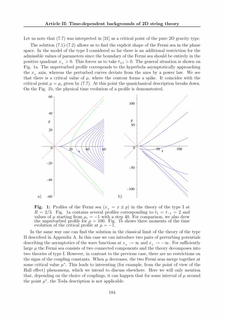
Article II: Time-dependent backgrounds of 2D string theory
Let us note that (7.7) was interpreted in [31] as a critical point of the pure 2D gravity type.
The solution (7.1)-(7.2) allows us to find the explicit shape of the Fermi sea in the phasespace. In the model of the type I considered so far there is an additional restriction for theadmissible values of parameters since the boundary of the Fermi sea should be entirely in thepositive quadrant x± > 0. This forces us to take t±1 > 0. The general situation is shown onFig. 1a. The unperturbed profile corresponds to the hyperbola asymptotically approachingthe x± axis, whereas the perturbed curves deviate from the axes by a power law. We seethat there is a critical value of µ, where the contour forms a spike. It coincides with thecritical point µ = µc given by (7.7). At this point the quasiclassical description breaks down.On the Fig. 1b, the physical time evolution of a profile is demonstrated.
a) –60
–40
–20
0
20
40
60
p
20 40 60x
b)
–100
–50
0
50
100
p
50 100x
Fig. 1: Profiles of the Fermi sea (x± = x ± p) in the theory of the type I atR = 2/3. Fig. 1a contains several profiles corresponding to t1 = t−1 = 2 andvalues of µ starting from µc = −1 with a step 40. For comparison, we also drewthe unperturbed profile for µ = 100. Fig. 1b shows three moments of the timeevolution of the critical profile at µ = −1.
In the same way one can find the solution in the classical limit of the theory of the typeII described in Appendix A. In this case we can introduce two pairs of perturbing potentialsdescribing the asymptotics of the wave functions at x± → ∞ and x± → −∞. For sufficientlylarge µ the Fermi sea consists of two connected components and the theory decomposes intotwo theories of type I. However, in contrast to the previous case, there are no restrictions onthe signs of the coupling constants. When µ decreases, the two Fermi seas merge together atsome critical value µ∗. This leads to interesting (for example, from the point of view of theHall effect) phenomena, which we intend to discuss elsewhere. Here we will only mentionthat, depending on the choice of couplings, it can happen that for some interval of µ aroundthe point µ∗, the Toda description is not applicable.
184

§8 Free energy of the perturbed background
8 Free energy of the perturbed background
As we mentioned, the perturbations considered above appear in a theory at the finite tem-perature T = 1/β, β = 2πR. The free energy per unit volume F is related to the partitionfunction Z by
Z = e−βF . (8.1)
The free energy is considered as a function of the chemical potential µ, so that the numberof fermions is given by
N = ∂F/∂µ. (8.2)
We have seen that any perturbation can be characterized by the profile of the Fermi sea.For a generic profile, the number of fermions is given by the volume of the domain in thephase space occupied by the Fermi liquid
N =1
2π
∫ ∫
Fermi sea
dx+dx− . (8.3)
It is implied that the integral is regularized by introducing a cut-off at distance√
Λ. For theunperturbed ground state (5.1), one reproduces from (8.2) and (8.3) the well known resultfor the (universal part of the) free energy
F =1
4πµ2 logµ. (8.4)
The authors of [7] identify the partition function (8.1) for the tachyon backgroundsstudied in sect. 6 with the τ -function of the Toda hierarchy, defined by (6.28). In thissection we will reproduce this statement by direct integration over the Fermi sea, adjustingthe above derivation of (8.4) to the case of a general profile of the form (6.36).
Since the change of variables described by eq. (6.30) is canonical (see eq. (6.32)), onecan rewrite the integral (8.3) as
N =1
2π
−µ∫
dE
ω+
(E)∫
ω−(E)
dω
ω. (8.5)
The limits of integration over ω are determined by the cut-off.6 If we put it at the distancex± =
√Λ, they can be found from the equations
x±(ω±(E), E) =√
Λ. (8.6)
Taking the derivative with respect to µ, we obtain
∂µN = − 1
2πlog
ω+(−µ)
ω−(−µ). (8.7)
6The integral over E is also bounded from below, but we do not need to specify the boundary explicitly.
185

Article II: Time-dependent backgrounds of 2D string theory
It is enough to keep only the leading order in the cut-off Λ for the boundary values ω±. From(8.6) and (6.30) we find to this order
ω± =(
Λeχ/R)±1/2
. (8.8)
Combining (8.7) and (8.8), we find
∂µN = − 1
2πlog Λ − 1
2πRχ. (8.9)
Taking into account the relation (8.2) between the free energy and N , we see that
F = − 1
βlog τ, β = 2πR. (8.10)
As a result, if we compactify the theory at the time circle of the length β, our free energycoincides with the logarithm of the Toda τ -function.
The perturbed flow of the Fermi liquid is non-stationary with respect to the physical timet associated with the original Hamiltonian H0. In sec. 5 we constructed a new Hamiltonian,which preserves the shape of the Fermi sea. The latter coincides with the phase-spacetrajectory (5.11) at E = −µ. Using the fact that ∂µH(x+, x−) = 0, one can check that
F = 〈H(x+, x−) + µ〉. (8.11)
Note that the function H(x+, x−) is obtained by solving the profile equations (6.36) withrespect to µ. One can see, looking at the large x± asymptotics of the profile equations, thatit can be written in the following compact form:
H(x+, x−) = H0 +∑
k≥1
k
R(tkHk + t−kH−k). (8.12)
Here the Hamiltonians Hn(x+ , x−;~t ) are given by equations (6.21), with ω and E expressedas functions of x+ and x− through eq. (6.30).
9 Conclusions
In this paper we studied the 2D string theory in the presence of arbitrarily strong tachyonicperturbations. In the matrix model language, we dealt with the singlet sector of the MQMdescribed by a system of free fermions in inverted quadratic potential. In the quasiclassicallimit the state of the system is described by the shape of the domain in the phase spaceoccupied by the fermionic liquid (the profile of the Fermi sea). In this limit we formulatedfunctional equations, which determine the shape of the Fermi sea, given its asymptotics attwo infinities. There is some analogy between our problem and the problem of conformalmaps studied in [32, 33, 34, 35].
This allows to calculate various physical quantities related to the perturbed shape, suchas the free energy of the compactified Euclidean theory, in terms of the parameters definingthe asymptotic shapes.
186

§10 Problems and proposals
For a particular case of perturbations generated by vertex operators (in- and out-goingwith discrete equally spaced imaginary energies), the system solves the Toda lattice hier-archy where the Toda “times” correspond to the couplings characterizing the asymptoticsof the profile of the Fermi sea. Using the “light cone” representation in the phase space,we developed the Lax formalism of the constrained Toda hierarchy, where the constraintcoincides with the string equation found recently in [12]. In the dispersionless limit, the Laxformalism reproduces the functional equations for the shape of the perturbed Fermi sea andallows to give a direct physical meaning to the Toda mathematical quantities. In particular,we identified the two spectral parameters of the Toda system with the two chiral coordinatesx± in the target phase space.
Let us list the other possible applications of our formalism:• Calculation of the tachyon scattering matrix for 2D string theory in nontrivial backgrounds.• Analysis of the systems with more complicated than Sine-Liouville backgrounds. In par-ticular, the quasiclassical analysis of the sections 4 and 7 are not limited to any lattice oftachyon charges and can be used for a mixture of any commensurate or non-commensuratecharges. It provides a way of studying the whole space of possible tachyonic backgrounds ofthe 2D string theory.• Investigation of the thermodynamics of the 2D string theory in Sine-Liouville type tachy-onic backgrounds characterized by a lattice of discrete Matsubara energies [30, 36]. This issupposed to be the thermodynamics of the dilatonic black hole, according to the conjectureof [3].• The type 2 theory can be used to model the situation where either two quantum Halldroplets approach each other or one droplet is about to split in two.
10 Problems and proposals
We list also some unsolved problems, which could be approached by our formalism:• To find the metric of the target space for the Sine-Liouville string theory.• To construct the discrete states of the 2D string theory (at any rational compactificationradius) in the framework of our formalism.• A few important unsolved problems concern the relation between the MQM and CFTformulations of the 2D string theory. We still don’t have a precise mapping of the vertexand vortex operators of the MQM to the corresponding operators of CFT, in spite of theuseful suggestions of the papers [37, 4]. As the result, we did not manage to match the Sine-Liouville/Black Hole correlators calculated by [3, 38, 39] from the CFT approach with thecorresponding correlators found in [11] from the Toda approach to the MQM. Another relatedquestion is how can the target space integrable structure be seen in the CFT formulation of2D string theory.• Description and quantitative analysis of the mixed (vertex&vortex) perturbations in the2D string theory by means of the MQM. We hope that the “light-cone” formalism might beappropriate to study such perturbations, in spite of the absence of integrability.7
7An interesting proposal to describe nontrivial string backgrounds on the CFT side was given long agoin [40] and elaborated in [41, 42]. It suggested to parameterize the moduli space of the 2D string theoryperturbed in both sectors, by a conifold. This structure may be hidden in the 3 matrix model proposed
187

Article II: Time-dependent backgrounds of 2D string theory
Finally, keeping in mind this interesting problem, let us propose here a 3-matrix modelwhose grand canonical partition function Z(µ, tn, tn) =
∑∞N=0 e
−2πRµNZN(tn, tn) is the gen-erating function of correlators for both types of perturbations: the parameters tn are thecouplings of the vortex operators, in the same way as tn’s are the couplings of the tachyon(vertex) operators throughout this paper. As usual, the chemical potential µ plays the roleof the string coupling. The partition function at fixed N is represented by the integral overtwo hermitian matrices X± and one unitary matrix, the holonomy factor Ω around the circle
ZN(tn, tn) =∫
[DX+]tn[DX−]t−n[dΩ]t±n eTr(X−X+−qX−ΩX+Ω−1), (10.1)
where we denoted q = ei2πR and introduced the following matrix integration measures
[dX±]t±n = dX± e∑
n>0t±n TrX
n/R± , (10.2)
[dΩ]t±n = [dΩ]SU(N)
e∑
n6=0tn TrΩn
. (10.3)
This 3-matrix integral is nothing but the Euclidean partition function of the upside-downmatrix oscillator on a circle of length 2πR with twisted periodic boundary conditionsX±(β) = Ω†X±(0)Ω, needed for the introduction of the winding modes (vortices) in theMQM model of the 2D string theory [14]. It is trivial to show that in particular case of alltn = 0 this 3-matrix model reduces to the model with only vortex perturbations of the paper[10]. It can be also shown [36] that in the case of all tn = 0 it reduces to the Euclideanversion of the model with only tachyonic perturbations studied in this paper. The crucialpoint here is that the sources for tachyon perturbations are introduced in a single point onthe time circle, similarly to the perturbation imposing the initial conditions on the wavefunction (5.3). The model (10.1) reduces the problem of the study of the backgrounds of thecompactified 2D string theory with arbitrary tachyon and winding sources, to a three-matrixintegral.
We learned from R. Dijkgraaf and C. Vafa that they discovered a similar Toda structurein the c = 1 type theory arising in connection to the topological strings.
Acknowledgements: We would like to thank A. Boyarsky, G. Moore, A. Sorin, C. Vafa,and especially P. Wiegmann for useful discussions. Two of the authors (V.K. and I.K.) thankthe string theory group of Rutgers University, where a part of the work was done, for thekind hospitality. This work of S.A. and V.K. was partially supported by European Unionunder the RTN contracts HPRN-CT-2000-00122 and -00131. The work of S.A. and I.K. wassupported in part by European network EUROGRID HPRN-CT-1999-00161.
Appendix A. Theory of type II
In the theory of type II, the fermions are defined on the whole real line. In this case oneshould introduce two sets of functions describing, in the quasiclassical limit, fermions at
below.
188

§A Theory of type II
different sides of the potential. They are defined on right (left) semi-axis by
ψE
±,>(x±) =
1√2π
x±iE− 1
2±√
1 + e2πE(x± > 0), (A.1)
ψE
±,<(x±) =
1√2π
(−x±)±iE− 12√
1 + e2πE(x± < 0) (A.2)
and the continuation to the other semi-axis is performed according to the rule x± → e∓πix±.This gives, for x± > 0
ψE
±,>(−x±) = ±ieπEψE
±,>(x±), (A.3)
ψE
±,<(x±) = ±ieπEψE
±,<(−x±). (A.4)
The functions (A.1) satisfy the orthonormality and completeness conditions
〈ψE
±,a|ψE′
±,b〉 = δabδ(E − E ′), (A.5)
∫ ∞
−∞dE
∑
a
ψE±,a
(x±)ψE
±,a(x′±) = δ(x± − x′±), (A.6)
where the indices a, b = (>,<) label the right and left wave functions and the scalar productis defined as in (4.5) but with the integral over the whole real axis.
The unitary operator relating x± representations is given by the Fourier kernel on thewhole line K(x− , x+) = 1√
2πeix+x−
[Sψ+ ](x−) =∫ ∞
−∞dx+ K(x− , x+)ψ+(x+). (A.7)
It acts on the eigenfunctions (A.1) by the following matrix
[
S±1ψE
±,a
]
(x∓) =∑
b
[S±1(E)]abψE
±,b(x∓), S(E) = R(E)
(
1 −ieπE−ieπE 1
)
, (A.8)
where
R(E) =1√2πe−
π2(E−i/2)Γ(iE + 1/2). (A.9)
In this case the reflection coefficient R(E) is not a pure phase because of the tunnelingthrough the potential described by the off-diagonal elements of the S-matrix. Nevertheless,the whole S-matrix is unitary
S†(E)S(E) = 1. (A.10)
The scalar product between left and right states is given by
〈ψ−|K|ψ+〉 =∫ ∞
−∞dx+dx− ψ−(x−)K(x− , x+)ψ+(x+). (A.11)
It is clear that the matrix of scalar products of states (A.1) coincides with S(E)δ(E − E ′).The corresponding completeness condition is
∫ ∞
−∞dE
∑
a,b
ψE−,a
(x−)(
S−1)
abψE
+,b(x+) =
1√2πe−ix+x− . (A.12)
189

Article II: Time-dependent backgrounds of 2D string theory
References
[1] V.A. Kazakov and A.A. Migdal, “Recent progress in the non-critical strings” Nucl.
Phys. B311 (1988) 171.
[2] E. Brezin, C. Itzykson, G. Parisi, and J.-B. Zuber, Comm. Math. Phys. 59 (1978) 35.
[3] V. Fateev, A. Zamolodchikov, and Al. Zamolodchikov, unpublished.
[4] J. Polchinski, “What is string theory”, Lectures presented at the 1994 Les Houches
Summer School “Fluctuating Geometries in Statistical Mechanics and Field Theory”,hep-th/9411028.
[5] A. Jevicki, “Developments in 2D string theory”, hep-th//9309115.
[6] G. Moore, M. Plesser, and S. Ramgoolam, “Exact S-matrix for 2D string theory”, Nucl.
Phys. B377 (1992) 143, hep-th/9111035.
[7] R.Dijkgraaf, G.Moore, and M.R.Plesser, “The partition function of 2d string theory”,Nucl. Phys. B394 (1993) 356, hep-th/9208031.
[8] G. Moore, “Gravitational phase transitions and the sine-Gordon model”,hep-th/9203061.
[9] J. Hoppe, V. Kazakov, and I. Kostov, “Dimensionally reduced SYM4 as solvable matrixquantum mechanics”, Nucl. Phys. B571 (2000) 479, hep-th/9907058.
[10] V. Kazakov, I. Kostov, and D. Kutasov, “A Matrix Model for the Two DimensionalBlack Hole”, Nucl. Phys. B622 (2002) 141, hep-th/0101011.
[11] S. Alexandrov and V. Kazakov, “Correlators in 2D string theory with vortex condensa-tion”, Nucl. Phys. B610 (2001) 77, hep-th/0104094.
[12] I. Kostov, “String Equation for String Theory on a Circle”, Nucl. Phys. B624 (2002)146, hep-th/0107247.
[13] D. Gross and I. Klebanov, Nucl. Phys. B344 (1990) 475; Nucl. Phys. B354 (1990) 459.
[14] D. Boulatov and V. Kazakov, “One-Dimensional String Theory with Vortices as Upside-Down Matrix Oscillator”, Int. J. Mod. Phys. 8 (1993) 809, hep-th/0012228.
[15] H.A. Fertig, Phys. Rev. B36 (1987) 7969.
[16] O. Agam, E. Bettelheim, P. Wiegmann, and A. Zabrodin, “Viscous fingering and ashape of an electronic droplet in the Quantum Hall regime”, Phys. Rev. Lett.88 (2002)236802, cond-mat/0111333.
[17] H.A. Fertig, Phys. Rev. B387 (1988) 996.
[18] I. Klebanov, Lectures delivered at the ICTP Spring School on String Theory and Quan-
tum Gravity, Trieste, April 1991, hep-th/9108019.
190

References
[19] E. Brezin, V. Kazakov and Al. Zamolodchikov, Nucl. Phys. B338 (1990) 673.
[20] G. Parisi, Phys. Lett. B238 (1990) 209, 213.
[21] D. Gross and N. Miljkovic, Phys. Lett. B238 (1990) 217.
[22] P. Ginsparg and J. Zinn-Justin, Phys. Lett. B240 (1990) 333.
[23] T. Eguchi and H. Kanno, “Toda lattice hierarchy and the topological description of thec = 1 string theory”, Phys. Lett. B331 (1994) 330, hep-th/9404056.
[24] T. Nakatsu, “On the string equation at c = 1”, Mod. Phys. Lett. A9 (1994) 3313,hep-th/9407096.
[25] K. Takasaki, “Toda lattice hierarchy and generalized string equations”, Comm. Math.
Phys. 181 (1996) 131, hep-th/9506089.
[26] A. Zabrodin, “Dispersionless limit of Hirota equations in some problems of complexanalysis”, Theor. Math. Phys. 129 (2001) 1511; Theor. Math. Phys. 129 (2001) 239,math.CV/0104169.
[27] K. Takasaki and T. Takebe, “Integrable Hierarchies and Dispersionless Limit”, Rev.
Math. Phys. 7 (1995) 743, hep-th/9405096.
[28] I. Krichever, Func. Anal. i ego pril., 22:3 (1988) 37 (English translation: Funct. Anal.
Appl. 22 (1989) 200); “The τ -function of the universal Witham hierarchy, matrix modelsand topological field theories”, Comm. Pure Appl. Math. 47 (1992), hep-th/9205110.
[29] K. Takasaki and T. Takebe, “Quasi-classical limit of Toda hierarchy and W-infinitysymmetries”, Lett. Math. Phys. 28 (93) 165, hep-th/9301070.
[30] V. A. Kazakov and A. Tseytlin, “On free energy of 2-d black hole in bosonic stringtheory”, JHEP 0106 (2001) 021, hep-th/0104138.
[31] E. Hsu and D. Kutasov, “The Gravitational Sine-Gordon Model”, Nucl. Phys. B396(1993) 693, hep-th/9212023.
[32] P. Wiegmann and A. Zabrodin, “Conformal maps and dispersionless integrable hierar-chies”, Comm. Math. Phys. 213 (2000) 523, hep-th/9909147.
[33] I. Kostov, I. Krichever, M. Mineev-Veinstein, P. Wiegmann, and A. Zabrodin, “τ -function for analytic curves”, Random matrices and their applications, MSRI publi-
cations 40 (2001) 285 (Cambridge University Press), hep-th/0005259.
[34] A. Boyarsky, A. Marshakov, O. Ruchhayskiy, P. Wiegmann, and A. Zabrodin, “Onassociativity equations in dispersionless integrable hierarchies”, Phys. Lett. B515 (2001)483, hep-th/0105260.
[35] M. Mineev-Weinstein, P. B. Wiegmann, A. Zabrodin, “Integrable Structure of InterfaceDynamics”, Phys. Rev. Lett.84 (2000) 5106, nlin.SI/0001007.
191
Article II: Time-dependent backgrounds of 2D string theory
[36] S. Yu. Alexandrov, V. A. Kazakov, I. K. Kostov, work in progress.
[37] G. Moore, N. Seiberg, and M. Staudacher, “From loops to states in 2D quantum grav-ity”, Nucl. Phys. B362 (1991) 665.
[38] J. Teschner, “The deformed two-dimensional black hole”, Phys. Lett. B458 (1999) 257,hep-th/9902189.
[39] T. Fukuda and K. Hosomichi, “Three-point Functions in Sine-Liouville Theory”, JHEP
0109 (2001) 003, hep-th/0105217.
[40] E. Witten, “Ground Ring of two dimensional string theory”, Nucl. Phys. B373 (1992)187, hep-th/9108004.
[41] S. Mukhi and C. Vafa, “Two dimensional black-hole as a topological coset model of c=1string theory”, Nucl. Phys. B407 (1993) 667, hep-th/9301083.
[42] D. Ghoshal and C. Vafa, “c=1 String as the Topological Theory of the Conifold”, Nucl.
Phys. B453 (1995) 121, hep-th/9506122.
192

Article III
Thermodynamics of 2D string theory
JHEP 0301 (2003) 078


SPHT-t02/158, LPTENS-02/54hep-th/0210251
Thermodynamics of 2D string theory
S. Yu. Alexandrov123 and V. A. Kazakov2
1 Service de Physique Theorique, CNRS - URA 2306, C.E.A. - Saclay,
F-91191 Gif-Sur-Yvette CEDEX, France2Laboratoire de Physique Theorique de l’Ecole Normale Superieure†
24 rue Lhomond, 75231 Paris Cedex 05, France3 V.A. Fock Department of Theoretical Physics, St. Petersburg University, Russia
We calculate the free energy, energy and entropy in the matrix quantum mechanical for-mulation of 2D string theory in a background strongly perturbed by tachyons with theimaginary Minkowskian momentum ±i/R (“Sine-Liouville” theory). The system shows athermodynamical behaviour corresponding to the temperature T = 1/(2πR). We show thatthe microscopically calculated energy of the system satisfies the usual thermodynamicalrelations and leads to a non-zero entropy.
†Unite de Recherche du Centre National de la Recherche Scientifique et de l’Ecole Normale Superieureet a l’Universite de Paris-Sud.

Article III: Thermodynamics of 2D string theory
1 Introduction
Nontrivial backgrounds in the string theory often have a thermodynamical behaviour corre-sponding to a certain temperature and a classically big entropy. Typical examples are theblack holes where the thermodynamics manifests itself by the Hawking radiation at a cer-tain temperature TH and the Bekenstein-Hawking entropy. The latter is expressed throughthe classical parameters of the system (the area of the horizon) and satisfies the standardthermodynamical relations with the free energy and energy (mass of the black hole).1
In this paper we will try to demonstrate that the thermodynamical behaviour with atemperature T is a rather natural phenomenon in the 2-dimensional string theory in spe-cific backgrounds created by tachyon sources with Euclidean momenta corresponding to theMatsubara frequencies 2πk/T, k = 1, 2, . . .. For k = 1 this system is T-dual to the so called“Sine-Liouville” theory conjectured to describe 2D string theory on the Euclidean black holebackground [3]. The latter can be obtained introducing a vortex source with the Euclideantime compactified on a radius R = 1/2πT . It was studied in [4] and further in [5, 6] in thematrix quantum mechanical (MQM) formulation using the integrability properties.
We will use here the MQM in the singlet sector to study this system in Minkowskiantime, perturbed by a source of “tachyons” with imaginary momenta. This approach, elabo-rated in the paper [7], using some early ideas of [8], extensively relies on the classical Todaintegrability and the representation of the system in terms of free fermions arising from theeigenvalues of the matrix field. We will demonstrate that the microscopically defined energyof the system, calculated as the energy of (perturbed) Fermi sea, coincides with its thermo-dynamical counterpart E calculated as the derivative of the free energy with respect to thetemperature. The free energy itself can be found from the Fermi sea due to its relation withthe number of particles N = ∂F/∂µ.
This coincidence of the microscopic and thermodynamical energies looks satisfactory,though a little bit mysterious to us. We could not figure out here where the entropy, alsofollowing from this derivation, comes from since the system looks like a single classical stateof the moving Fermi liquid. The formulas become especially simple in the black hole limitproposed in [4], where the energy and entropy dominate with respect to the free energy. Onthe other hand, the entropy naturally disappears in the opposite limit of the trivial lineardilaton background where the perturbation source is absent.
The entropy seems to be more visible in the T-dual formulation of the theory basedon the vortex perturbation in the compact Euclidean time where we deal with the higherrepresentations of the SU(N) symmetry of the MQM [9]. However the direct counting ofthe nonsinglet states appears to be technically a difficult problem. But we still think thatour observation could shed light on the origin of the entropy of the black hole type solutionsin the string theory.
The paper is organized as follows. In the next section we review the fermionic repre-sentation of c = 1 string theory. In section 3 we show how one can describe the tachyonperturbations in this formalism. Section 4 presents the explicit solution for the particularcase of the Sine-Liouville theory. In section 5 we evaluate the grand canonical free energyand energy of the system using the techniques of integration over the Fermi sea. In section 6
1For review of black hole physics see [1, 2].
196

§2 The c = 1 string theory as the collective theory of the Fermi sea
we demonstrate that the quantities found in the previous section satisfy the thermodynami-cal relations and give rise to a nonvanishing entropy. The parameter R of the perturbationscan be interpreted as the inverse temperature. Finally, we discuss our results and remainingproblems.
2 The c = 1 string theory as the collective theory of the
Fermi sea
The c = 1 string theory can be formulated in terms of collective excitations of the Fermi seaof the upside-down harmonic oscillator [10, 11, 12, 13]. The tree-level tachyon dynamics ofthe string theory is contained in the semiclassical limit of the ensemble of fermions, in whichthe fermionic density in the phase space is either one or zero. Each state of the string theorycorresponds to a particular configuration of the incompressible Fermi liquid [14, 15, 16].
In the quasi-classical limit the motion of the fermionic liquid is determined by the classicaltrajectories of its individual particles in the phase space. It is governed by the one-particleHamiltonian
H0 =1
2
(
p2 − x2)
, (2.1)
where the coordinate of the fermion x stands for an eigenvalue of the matrix field andp = −i ∂
∂xis its conjugated momentum. We introduce the chiral variables
x±(t) =x(t) ± p(t)√
2, (2.2)
and define the Poisson bracket as f, g = ∂f∂x−
dg∂x+
− ∂f∂x+
dg∂x−
. In these variables H0 = −x+x−
and the equations of motion have a simple solution
x±(t) = e±tx± , (2.3)
where the initial values z± parameterize the points of the Fermi sea. Each trajectory rep-resents a hyperbole H0(p, x) = E. The state of the system is completely characterized bythe profile of the Fermi sea that is a curve in the phase space which bounds the region filledby fermions. For the ground state, the Fermi sea is made by the classical trajectories withE < −µ, and the profile is given by the hyperbole
x+x− = µ. (2.4)
The state is stationary since the Fermi surface coincides with one of the classical trajectoriesand thus the form of the Fermi sea is preserved in time. For an arbitrary state of the Fermisea, the Fermi surface can be defined more generally by
x+x− = M(x+ , x−). (2.5)
It is clear from (2.3) that a generic function M in (2.5) leads to a time-dependent profile.However, this dependence is completely defined by (2.3) and it is of little interest to us. Wecan always replace (2.5) by the equation for the initial values x± .
197

Article III: Thermodynamics of 2D string theory
For a given profile, we define the energy of the system and the number of fermions as thefollowing integrals over the Fermi sea
E0 =1
2π
∫ ∫
Fermi sea
dx dp H0(x, p), N =1
2π
∫ ∫
Fermi sea
dx dp. (2.6)
It is implied that the integrals are bound by a cut-off at a distance√
2Λ. For example, we canrestrict the integration to 0 < z± <
√Λ. For the ground state (2.4), dropping non-universal
terms proportional to the cut-off one reproduces the well known result [17]
E0(µ) = − 1
4πµ2 log(µ/Λ), N(µ) =
1
2πµ log(µ/Λ). (2.7)
Given the number of fermions, one can also introduce the grand canonical free energythrough the relation
N = ∂F/∂µ, (2.8)
where F is given in terms of the partition function for a time interval T by
F = − logZ/T. (2.9)
For the case of the ground state, one finds from (2.7) that the (universal part of the) grandcanonical free energy is related to the energy of the fermions as
F = E0 + µN =1
4πµ2 log(µ/Λ). (2.10)
3 The profile of the Fermi sea for time dependent
tachyon backgrounds
The ground state (2.4) describes the simplest, linear dilaton background of the bosonic string.Now we would like to study more general backgrounds characterized by condensation oftachyons with nonzero momenta. Such backgrounds correspond to time-dependent profiles(2.5), characterized by the function M(x+ , x−). We restrict ourselves to the states thatcontain only tachyon excitations whose momenta belong to a discrete lattice
pn = in/R, n ∈ Z. (3.1)
They look as Matsubara frequencies corresponding to the temperature T = 1/(2πR), or tothe compactification in the Euclidean time with the radius R. We will perturb the system inthe same manner as in [7]. It has been shown that at the quasiclassical level the perturbationscan be completely characterized by the asymptotics of the profile of the Fermi sea at x+ x−
and x− x+. Accordingly, the equation for the profile can be written in two forms whichshould be compatible with each other [7]
x+x− = M±(x±) =1
R
n∑
k=1
kt±kxk/R± + µ+
1
R
∞∑
k=1
v±kx−k/R± , (3.2)
198

§4 Solution for Sine-Gordon coupled to gravity
where t±k are coupling constants associated with the perturbing operators and defining theasymptotics of the Fermi sea for z+ z− and z− z+ correspondingly. v±k are thecoefficients to be found, which completely fix the form of the profile.
It was shown in [7] that such perturbations are described by the dispersionless limit ofa constrained Toda hierarchy. The phase space coordinates x± play the role of the Laxoperators, t±k are the Toda times, and eq. (3.2) appears as the constraint (string equation)of the hierarchy [6].
The integrability allows to find the explicit solution for the profile. It is written in theparametric form as follows
x±(ω, µ) = e−1
2Rχ(µ)ω±1
(
1 +n∑
k=1
a±k(µ) ω∓k/R)
, (3.3)
where χ is the so called string susceptibility related to the Toda τ -function as χ = ∂2µ log τ .
The latter is the generating function for the coefficients v±k in (3.2)
v±k = ∂t±klog τ, (3.4)
which can be identified with one-point vertex correlators [5, 7]. Moreover, the change ofvariables x± → logω, µ turns out to be canonical, i.e.,
µ, logω = 1. (3.5)
To find the coefficients a±k it is enough to use a simple procedure suggested in [6]. One shouldsubstitute the expressions (3.3) in the profile equations (3.2) and compare the coefficients infront of ω±k/R.
4 Solution for Sine-Gordon coupled to gravity
Let us restrict ourselves to the case n = 1 corresponding to the Sine-Gordon theory coupledto gravity or the so called Sine-Liouville theory. In this case there are only t±1 couplingconstants and the equation (3.3) takes the form [5]
x± = e−1
2Rχω±1(1 + a±ω
∓ 1R ), (4.1)
where χ can be found from [4, 18]
µe1Rχ +
1
R2
(
1
R− 1
)
t1t−1e2R−1
R2 χ = 1, a± =t∓1
Re
2R−1
2R2 χ. (4.2)
Assuming that 12< R < 1 (which means that the corresponding compactification radius is
between the Kosterlitz-Thouless and the self-dual one), the first equation for the sucsept-ability can also be rewritten in terms of scaling variables:
w = µξ, ξ =
(
λ
R
√
1/R− 1
)− 2R2R−1
, (4.3)
where λ =√t1t−1. The result reads
χ = R log ξ +X(w),
w = e−1RX − e−
R−1R
X . (4.4)
199

Article III: Thermodynamics of 2D string theory
5 Free energy and energy of the perturbed background
Let us consider the average over the Fermi sea of an observable O defined on the phase space
< O >=1
2π
∫ ∫
Fermi sea
dx+dx− O(x+, x−). (5.1)
Here the boundary of the integration is defined by the profile equation (3.2). Since thechange of variables described by eq. (3.3) is canonical (see eq. (3.5)), one can write
< O >=1
2π
∫
µ
ds
ω+
(s)∫
ω−(s)
dω
ωO(x+(ω, s), x−(ω, s)). (5.2)
The limits of integration over ω are defined by the cut-off. We choose it as two walls atx+ =
√Λ and x− =
√Λ. Then the limits can be found from the equations
x±(ω±(s), s) =√
Λ. (5.3)
First, consider the case of O = 1. Then the integral (5.1) gives the number of fermionsin the Fermi sea, i.e., N =< 1 >. Taking the derivative with respect to µ, we obtain
∂µN = − 1
2πlog
ω+(µ)
ω−(µ). (5.4)
In this case it is enough to restrict ourselves to the main order in the cut-off Λ for theboundary values ω±. From (5.3) and (3.3) we find to this order
ω± = ω±1(0) , ω(0) =
√Λeχ/R. (5.5)
Combining (5.4) and (5.5), we find
∂µN = − 1
2πlog Λ − 1
2πRχ. (5.6)
Taking into account the relation (2.8), we find that the free energy coincides with the log-arithm of the τ -function and β = 2πR represents the time interval at which the theory iscompactified
F = − 1
βlog τ. (5.7)
This derivation of the grand canonical free energy was done in [7]. However, using thegeneral formula (5.2), we can also find the energy of the system, at least for the case of theSine-Liouville theory. Since it is given by the integral of the free Hamiltonian (2.6), from(5.2) and (4.1) one obtains
∂µE = −∂µ < x+x− >=1
2πe−
1Rχ
(1 + a+a−) logω − Ra+ω−1/R +Ra−ω
1/R
∣
∣
∣
∣
ω+
ω−
. (5.8)
200
§6 Thermodynamics of the system
To find the final expression one needs to know the limits ω± in the second order in the cut-off.It is easy to show from (5.3) that eq. (5.5) should be changed by
ω± = ω±1(0)(1 ∓ a±ω
−1/R(0) ). (5.9)
Substituting these limits into (5.8), one finds
∂µE =1
2πe−
1Rχ
(1 + a+a−)(
log Λ +1
Rχ)
− 2a+a−
+R
2π(t1 + t−1)Λ
1/2R. (5.10)
Integrating over µ and using a+a− = R1−Re
2R−1
R2 X , we get
2πE = ξ−2
(
1
2Re−
2RX +
2R− 1
R(1 −R)e−X − 1
2(1 − R)e−2 R−1
RX
)
(χ +R log Λ)
+ ξ−2
(
1
4e−
2RX − R
1 − Re−X +
R(4 − 5R)
4(1 − R)2e−2 R−1
RX
)
+R(t1 + t−1)µΛ1/2R.(5.11)
We observe that the last term is non-universlal since it does not contain a singularity atµ = 0. However, log Λ enters in a non-trivial way. It is combined with a non-trivial functionof µ and ξ.
6 Thermodynamics of the system
We found above the energy of the Sine-Liouville theory (5.11) and also restored the freeenergy in the grand canonical ensemble for a general perturbation. In the Sine-Liouville caseone can integrate the equation (4.4) to get the explicit expression [4]
2πF = − 1
2Rµ2(χ+R log Λ)− ξ−2
(
3
4e−
2RX − R2 − R + 1
1 −Re−X +
3R
4(1 −R)e−2 R−1
RX
)
. (6.1)
Now we are going to establish thermodynamical properties of our system. It is expected topossess them since the spectrum of perturbations corresponds to the Matsubara frequenciestypical for a system at a nonzero temperature. First of all, note that in the standardthermodynamical relations the free energy appears in the canonical, rather than in grandcanonical ensemble. Therefore we define
F = F − µ∂F∂µ
. (6.2)
It is easy to check that it can be written as
2πF =1
R
∫ µ
sχ(s)ds =1
2Rµ2(χ +R log Λ)
+ ξ−2
(
1
4e−
2RX − Re−X +
R
4(1 − R)e−2 R−1
RX
)
. (6.3)
Following the standard thermodynamical relations, let us also introduce the entropy as adifference of the energy and the free energy:
S = β(E − F ). (6.4)
201

Article III: Thermodynamics of 2D string theory
One finds from (5.11) and (6.3)
S = ξ−2
(
R
1 − Re−X − 1
2(1 −R)e−2 R−1
RX
)
(χ+R log Λ)
+ ξ−2
(
− R3
1 −Re−X +
R2(3 − 4R)
4(1 − R)2e−2 R−1
RX
)
+R2
2π(t1 + t−1)µΛ1/2R. (6.5)
Thus, all quantities are supplied by a thermodynamical interpretation. The role of thetemperature is played by T = β−1 = 1/2πR. However, to have a consistent picture, thefollowing (equivalent) thermodynamical relations should be satisfied:
S = −∂F∂T
= 2πR2∂F
∂R,
E =∂(βF )
∂β=∂(RF )
∂R. (6.6)
In these relations it is important which parameters are hold to be fixed when we evaluatethe derivatives with respect to R. Since we use the free energy in the canonical ensemble,one should fix the number of fermions N and the coupling constant λ but not the chemicalpotential µ.
Another subtle point is that a priori the relation of our initial parameters to the corre-sponding parameters which are to be fixed may contain a dependence on the inverse tem-perature R. Therefore, in general we should redefine
ξ −→ ξ = (a(R)λ)−2
2−R ,
Λ −→ b(R)Λ, (6.7)
F −→ F +1
2c(R)µ2.
We find the functions a(R), b(R) and c(R) from the condition (6.6), where N , λ and Λ arefixed. We emphasize that it looks rather non-trivial to us that it is possible to find such func-tions of R that this condition is satisfied. It can be considered as a remarkable coincidenceindicating that the functions F , E and S do have the interpretation of thermodynamicalquantities as free energy, energy and entropy correspondingly. In appendix A it is shownthat the parameters should be taken as
a(R) =(
1 − R
R3
)1/2
, b(R) = 1, c(R) = 0. (6.8)
It is worth noting several features of this solution. First of all, the plausible property isthat we do not redefine the cut-off and the free energy. Moreover, the constant λ coincideswith its initial definition (4.3) what probably indicates that λ is correctly identified with thecorresponding coupling constant in the conformal Sine-Liouville theory. Another importantconsequence of the choice (6.8) is that the entropy (6.5) is proportional to λ2 and thereforevanishes in the absence of perturbations. It appears to be non-zero only when the backgroundof the string theory is described by a time dependent Fermi sea. However, a puzzle stillremains how to calculate the entropy in a similar way as the energy was evaluated, thatis by directly identifying the corresponding degrees of freedom which give rise to the samemacroscopic state and, hence, the entropy.
202
§7 Conclusions and problems
6.1 The ”Black hole” limit
Let us restrict ourselves to the limit µ → 0. If we perturbed the 2D string theory by thevortex, instead of the tachyon, modes it would correspond to the black hole limit [3, 4]. Inthis limit we have X = 0. As a result, we obtain from (6.3), (5.11) and (6.5) for all threethermodynamical quantities:
2πF =(2R− 1)2
4(1 − R)λ
4R2R−1 ,
2πE =2R− 1
2R(1 − R)
(
log(Λξ) − R
2(1 −R)
)
λ4R
2R−1 , (6.9)
S =2R− 1
2(1 − R)
(
log(Λξ) − R2(3 − 2R)
2(1 −R)
)
λ4R
2R−1 ,
where λ = a(R)λ. It is worth to note an interesting feature of this solution. Since log(Λξ) 1, we get 2πE ≈ S and in comparison with these quantities F is negligible. This is to becompared with the result of [19] that the analysis of the dilatonic gravity derived from 2Dstring theory leads to the vanishing free energy and to the equal energy and entropy. Wesee that it can be true only in a limit, but the free energy can never be exactly zero sinceit is its derivative with respect to the temperature that produces all other thermodynamicalquantities.
For the special case of R = 2/3 which is T-dual to the stringy black hole model, we find:
βF =1
18λ8,
βE =(
1
2log(Λξ) − 1
2
)
λ8, (6.10)
S =(
1
2log(Λξ) − 5
9
)
λ8.
For the dual compactification radius R = 3/2, all quantities change their sign:
βF = −3λ3,
βE = − (2 log(Λξ) − 3) λ3, (6.11)
S = −2 log(Λξ)λ3.
This might be interpreted as a result for the background dual to the black hole of a negativemass, which does appear in the analysis of [20].
7 Conclusions and problems
The main puzzle of the black hole physics is to find the states corresponding to the entropyof a classical gravitating system. In our case, instead of a black hole, the role of such systemis played by a nontrivial tachyonic background. However, it manifests the similar propertiesas the usual dilatonic black hole, which appears as a T-dual perturbation of the initial
203

Article III: Thermodynamics of 2D string theory
flat spacetime. Therefore, it is not surprising that the studied background also possesses anonvanishing entropy.
In our case we have a little more hope to track the origin of the entropy, than, forexample, in the study of the Schwarzschild black hole, since we are dealing with the welldefined string theory and can identify its basic degrees of freedom. It allowed us in thispaper to find microscopically the energy and free energy of the “Sine-Liouville” background.The entropy was calculated not independently, but followed from the basic thermodynamicalrelations. Our main result is the coincidence of this microscopic and the thermodynamicalenergies. The latter is calculated as a derivative of the free energy with respect to thetemperature. Note that the “temperature” appears from the very beginning as a parameterof the tachyonic perturbation, and not as a macroscopic characteristic of a heated system.That is why the thermodynamical interpretation comes as a surprise.
An analogous situation can be seen in the Unruh effect [21]. There the temperature seenby the accelerating observer is defined by the value of the acceleration, which does not a
priory have any relation to thermodynamics. In fact, in the latter case the temperaturecan be found from the analysis of the quantum field theory on the Rindler space which isthe spacetime seen by the accelerating observer. The same should be true for our case. Itshould be possible to reproduce the global structure of the tachyonic background from thematrix model solution, and then the thermodynamical interpretation should appear fromthe analysis of the spectrum of particles detected by some natural observer [22].
One might try to find a hint to the thermodynamical behaviour of our system in thevery similar results for the T-dual system of [4] where instead of tachyons we have theperturbation by vortices. There the Euclidean time is compactified from the very beginningand the Gibbs ensemble is thus explicitly introduced with R as a temperature parameter. Onthe other hand, the coincidence of microscopic energies in two mutually dual formulations(up to duality changes in parameters, like R → 1/R) is far from obvious. Even how to findthe energy in this dual case is not clear.
In conclusion, we hope that our observation will help to find a microscopic approachto the calculation of entropy at least in the 2D string theory with nontrivial backgrounds.Together with the plausible conjecture that the dual system describes the 2D dilatonic blackhole, it could open a way for solving the puzzle of the microscopic origin of entropy in theblack hole physics.
Acknowledgements: The authors are grateful I. Kostov for valuable discussions. Alsowe thank the Theoretical Physics Division of CERN, where a part of the work was done,for the kind hospitality. This work of S.A. and V.K. was partially supported by EuropeanUnion under the RTN contracts HPRN-CT-2000-00122 and -00131. The work of S.A. wassupported in part by European network EUROGRID HPRN-CT-1999-00161.
204

§A Calculation of ∂F/∂R
Appendix A. Calculation of ∂F/∂R
In this appendix we calculate the derivative of the free energy (6.3) with respect to R. First,note that due to (6.2) and (2.8), we have
(
∂F
∂R
)
N,λ,Λ
=
(
∂F∂R
)
µ,λ,Λ
=
(
∂F∂R
)
µ,ξ,Λ
+
(
∂ξ
∂R
)
λ
(
∂F∂ξ
)
µ,Λ,R
. (A.1)
From (6.1) and (6.7) one can obtain
2πξ
(
∂F∂ξ
)
µ,Λ,R
= −ξ−2R(2R− 1)
1 − R
(
e−X − 1
2Re−2 R−1
RX)
, (A.2)
ξ−1
(
∂ξ
∂R
)
λ
= − 1
R(2R− 1)
(
log ξ + 2R2d log a(R)
dR
)
. (A.3)
The most complicated contribution comes from the first term in (A.1). From (6.1), (6.7)and (4.4) one finds
2π
(
∂F∂R
)
µ,ξ,Λ
= ξ−2
(
1
1 − Re−X − 1
2R(1 −R)e−2 R−1
RX
)
X
R
+ ξ−2
(
R(2 − R)
(1 −R)2e−X − 3
4(1 − R)2e−2 R−1
RX
)
− 1
2µ2
(
d log b(R)
dR+dc(R)
dR
)
. (A.4)
Putting the results (A.2), (A.3) and (A.4) together, we obtain
2π
(
∂F
∂R
)
N,λ,Λ
=1
R2ξ−2
(
R
1 −Re−X − 1
2(1 − R)e−2 R−1
RX
)
χ
+ ξ−2
(
R(2 − R)
(1 − R)2e−X − 3
4(1 −R)2e−2 R−1
RX
)
+ ξ−2
(
2R2
1 − Re−X − R
1 − Re−2 R−1
RX
)
d log a(R)
dR
− 1
2µ2
(
d log b(R)
dR+dc(R)
dR
)
. (A.5)
We observe that the term proportional to the susceptibility χ coincides with the correspond-ing term in the entropy (6.5) what can be considered as the main miracle of the presentderivation. To get the coincidence of other terms, we obtain a system of three equations,from which only two are independent:
d log b(R)
dR+dc(R)
dR= 0,
2d log a(R)
dR− 1
R2log b(R) =
2R− 3
R(1 −R). (A.6)
205

Article III: Thermodynamics of 2D string theory
Since we have only two equations on three functions, there is an ambiguity in the solution.It can be fixed if we require that the entropy vanishes without perturbations. Then we cometo the following result
a(R) =(
1 −R
R3
)1/2
, log b(R) = 0, c(R) = 0, (A.7)
which ensures the thermodynamical relations (6.6). Note that in fact they are fulfilledonly up to terms depending on the cut-off log Λ. Such terms can not be reproduced bydifferentiating with respect to the temperature, but they are considered as non-universal inour approach and thus can be dropped.
References
[1] W. Kummer and D. V. Vassilevich, “Hawking radiation from dilaton gravity in (1+1)dimensions: A pedagogical review”, Annalen Phys. 8 (1999) 801, gr-qc/9907041.
[2] S. R. Das and S. D. Mathur, ‘’The Quantum Physics of Black Holes: Results fromString Theory”, Ann. Rev. Nucl. Part. Sci. 50 (2000) 153, gr-qc/0105063.
[3] V. Fateev, A. Zamolodchikov, and Al. Zamolodchikov, unpublished.
[4] V. Kazakov, I. Kostov, and D. Kutasov, “A Matrix Model for the Two DimensionalBlack Hole”, Nucl. Phys. B622 (2002) 141, hep-th/0101011.
[5] S. Alexandrov and V. Kazakov, “Correlators in 2D string theory with vortex condensa-tion”, Nucl. Phys. B610 (2001) 77, hep-th/0104094.
[6] I. Kostov, “String Equation for String Theory on a Circle”, Nucl. Phys. B624 (2002)146, hep-th/0107247.
[7] S.Yu. Alexandrov, V.A. Kazakov, and I.K. Kostov, “Time-dependent backgrounds of2D string theory”, Nucl. Phys. B640 (2002) 119, hep-th/0205079.
[8] R.Dijkgraaf, G.Moore, and M.R.Plesser, “The partition function of 2d string theory”,Nucl. Phys. B394 (1993) 356, hep-th/9208031.
[9] V. A. Kazakov and A. Tseytlin, “On free energy of 2-d black hole in bosonic stringtheory”, JHEP 0106 (2001) 021, hep-th/0104138.
[10] E. Brezin, V. Kazakov and Al. Zamolodchikov, Nucl. Phys. B338 (1990) 673.
[11] G. Parisi, Phys. Lett. B238 (1990) 209, 213.
[12] D. Gross and N. Miljkovic, Phys. Lett. B238 (1990) 217.
[13] P. Ginsparg and J. Zinn-Justin, Phys. Lett. B240 (1990) 333.
206

References
[14] J. Polchinski, “What is string theory”, Lectures presented at the 1994 Les Houches
Summer School “Fluctuating Geometries in Statistical Mechanics and Field Theory”,hep-th/9411028.
[15] I. Klebanov, Lectures delivered at the ICTP Spring School on String Theory and Quan-
tum Gravity, Trieste, April 1991, hep-th/9108019.
[16] A. Jevicki, “Developments in 2D string theory”, hep-th//9309115.
[17] V.A. Kazakov and A.A. Migdal, “Recent progress in the non-critical strings” Nucl.
Phys. B311 (1988) 171.
[18] G. Moore, “Gravitational phase transitions and the sine-Gordon model”,hep-th/9203061.
[19] C. R. Nappi and A. Pasquinucci, “Thermodynamics of two-dimensional black holes”,Mod. Phys. Lett. A7 (1992) 3337, hep-th/9208002.
[20] R. Dijkgraaf, E. Verlinde, and H. Verlinde, “String propagation in a black hole geome-try”, Nucl. Phys. B371 (1992) 269.
[21] S. R. Unruh, ‘’Notes on black hole evaporation”, Phys. Rev. D14 (1976) 870.
[22] S.Yu. Alexandrov, in progress.
207


Article IV
2D String Theory as Normal
Matrix Model
Nucl. Phys. B667 (2003) 90

LPTENS-03/05, SPHT-t03/013, RUNHETC-2003-04hep-th/0302106
2D String Theory as Normal Matrix Model
Sergei Yu. Alexandrov,123 Vladimir A. Kazakov14, and Ivan K. Kostov1∗
1Laboratoire de Physique Theorique de l’Ecole Normale Superieure,†
24 rue Lhomond, 75231 Paris CEDEX, France2Service de Physique Theorique, CNRS - URA 2306, C.E.A. - Saclay,
F-91191 Gif-Sur-Yvette CEDEX, France3V.A. Fock Department of Theoretical Physics, St. Petersburg University, Russia
4Dept. of Physics and Astronomy, Rutgers University,
Piscataway NJ 08855 USA
We show that the c = 1 bosonic string theory at finite temperature has two matrix-modelrealizations related by a kind of duality transformation. The first realization is the standardone given by the compactified matrix quantum mechanics in the inverted oscillator potential.The second realization, which we derive here, is given by the normal matrix model. Bothmatrix models exhibit the Toda integrable structure and are associated with two dual cycles(a compact and a non-compact one) of a complex curve with the topology of a sphere withtwo punctures. The equivalence of the two matrix models holds for an arbitrary tachyonperturbation and in all orders in the string coupling constant.
∗Associate member of Institut za dreni Izsledvami i drena Energetika, BulgarianAcadrmy of Sciences, Sofia, Bulgaria
†Unite de Recherche du Centre National de la Recherche Scientifique et de l’Ecole Normale Superieureet a l’Universite de Paris-Sud.

Article IV: 2D String Theory as Normal Matrix Model
1 Introduction
The c = 1 string theory1 has been originally constructed in the early 90’s as the theory ofrandom surfaces embedded into a one-dimensional spacetime [2]. Since then it became clearthat this is only one of the realizations of a more universal structure, which reappeared invarious mathematical and physical problems. Most recently, it was used for the descriptionof the 2D black hole [3, 4, 5, 6] in the context of the topological string theories on Calabi-Yaumanifolds with vanishing cycles [7] and N = 1 SYM theories [8].
The c = 1 string theory can be constructed as the collective field theory for a one-dimensional N ×N hermitian matrix field theory known also as Matrix Quantum Mechanics
(MQM). This construction represents the simplest example of the strings/matrix correspon-dence. The collective excitations in the singlet sector of MQM are massless ”tachyons” withvarious momenta, while the non-singlet sectors contain also winding modes.
The singlet sector of MQM can be reduced to a system of N nonrelativistic fermions inthe upside-down gaussian potential. Thus the elementary excitations of the c = 1 stringcan be represented as collective excitations of free fermions near the Fermi level. The tree-level string-theory S-matrix can be extracted by considering the propagation of infinitesimal“pulses” along the Fermi sea and their reflection off the “Liouville wall” [9, 10]. The (time-dependent) string backgrounds are associated with the possible profiles of the Fermi sea[11].
An important property of the c = 1 string theory is its integrability. The latter has beendiscovered by Dijkgraaf, Moore and Plesser [12] in studying the properties of the tachyonscattering amplitudes. It was demonstrated in [12] that the partition function of the c = 1string theory in the case when the allowed momenta form a lattice, as in the case of thecompactified Euclidean theory, is a tau function of Toda hierarchy [13]. The operatorsassociated with the momentum modes in the string theory have been interpreted in [12] asToda flows. A special case represents the theory compactified at the self-dual radius R = 1.It is equivalent to a topological theory that computes the Euler characteristic of the modulispace of Riemann surfaces [14]. When R = 1 and only in this case, the partition function ofthe string theory has alternative realization as a Kontsevich-type model [12, 15].
In this paper we will show that there is another realization of the c = 1 string theoryby the so-called Normal Matrix Model (NMM). This is a complex N × N matrix model inwhich the integration measure is restricted to matrices that commute with their hermitianconjugates. The normal matrix model has been studied in the recent years in the context ofthe laplacian growth problem, the integrable structure of conformal maps, and the quantumHall droplets [16, 17, 18, 19, 20, 21]. It has been noticed that both matrix models, thesinglet sector of MQM and NMM, have similar properties. Both models can be reduced tosystems of nonrelativistic fermions and possess Toda integrable structure. There is howeveran essential difference: the normal matrix model describes a compact droplet of Fermi liquidwhile the Fermi sea of the MQM is non-compact. Furthermore, the perturbations of NMMare introduced by a matrix potential while these of MQM are introduced by means of time-dependent asymptotic states. In this paper we will show that nevertheless these two modelsare equivalent.
1As a good review we recommend [1].
212

§2 MQM, free fermions and integrability
The exact statement is that the matrix quantum mechanics compactified at radius Ris equivalent to the normal matrix model defined by the probability distribution functionexp[− 1
hWR(Z,Z†)], where
WR(Z,Z†) = tr (ZZ†)R − hR − 1
2tr log(ZZ†) −
∑
k≥1
tk trZk −∑
k≥1
t−k trZ†k. (1.1)
More precisely, the grand canonical partition function of MQM is identical to the canonicalpartition function of NMM at the perturbative level, by which we mean that the genusexpansions of the two free energies coincide. This will be proved in two steps. First, we willshow that the non-perturbed partition functions are equal. Then we will use the fact thatboth partition functions are τ -functions of Toda lattice hierarchy, which implies that theyalso coincide in presence of an arbitrary perturbation.
We also give a unified geometrical description of the two models in terms of a complexcurve with the topology of a sphere with two punctures. This complex curve is analog of theRiemann surfaces arising in the case of hermitian matrix models. However, for generic R itis not an algebraic curve. The curve has two dual non-contractible cycles, which determinethe boundaries of the supports of the eigenvalue distributions for the two models. Thenormal matrix model is associated with the compact cycle while the MQM is associatedwith the non-compact cycle connecting the two punctures. We will construct a globallydefined one-form whose integrals along the two cycles give the number of eigenvalues N andthe derivative of the free energy with respect to N .
The paper is organized as follows. In the next section we will remind the realization ofthe c = 1 string theory as a fermionic system with chiral perturbations worked out in [11].We will stress on the calculation of the free energy, which will be needed to establish theequivalence with the NMM. In Sect. 3 we construct the NMM having the same partitionfunction. In Sect. 4 we consider the quasiclassical limit and give a unified geometricaldescription of the two models.
2 MQM, free fermions and integrability
2.1 Eigenfunctions and fermionic scattering
In absence of winding modes, the 2D string theory is described by the singlet sector of MatrixQuantum Mechanics in the double scaling limit with Hamiltonian
H0 =1
2tr (−h2 ∂2
∂M2−M2). (2.1)
The radial part of this Hamiltonian is expressed in terms of the eigenvalues x1, . . . , xN of thematrix M . The wave functions in the SU(N)-singlet sector are completely antisymmetricand thus describe a system of N nonrelativistic fermions in the inverse gaussian potential.The dynamics of the fermions is governed by the Hamiltonian
H0 =1
2
N∑
i=1
(p2i − x2
i ), (2.2)
213

Article IV: 2D String Theory as Normal Matrix Model
where pi are the momenta conjugated to the fermionic coordinates xi.To describe the incoming and outgoing tachyonic states, it is convenient to introduce the
”light-cone” coordinates in the phase space
x± =x± p√
2(2.3)
satisfying the canonical commutation relations
[x+ , x−] = −ih. (2.4)
In these variables the one-particle Hamiltonian takes the form
H0 = −1
2(x+x− + x− x+). (2.5)
We can work either in x+ or in x− representation, where the theory is defined in termsof fermionic fields ψ±(x±) respectively. The solutions with a given energy are ψE
± (x± , t) =
e−ihEtψE
±(x±) with
ψE
± (x±) =1√2πh
e∓i
2hφ0x±
ihE− 1
2± , (2.6)
where the phase factor φ0(E) will be determined below. These solutions form two completesystems of δ-function normalized orthonormal states under the condition that the domainof the definition of the wave functions is a semi-axis.2 The left and right representations arerelated to each other by a unitary operator which is the Fourier transform on the half-line
[Sψ+ ](x−) =∫ ∞
0dx+ S(x−, x+)ψ+(x+). (2.7)
The integration kernel S(x−, x+) is either a sine or a cosine depending on the boundaryconditions at the origin. For definiteness, let us choose the cosine kernel
S(x− , x+) =
√
2
πhcos(
1
hx+x−). (2.8)
Then the operator S is diagonal on the eigenfunctions (2.6) with given energy
[SψE
+](x−) = e−
ihφ0R(E)ψE
− (x−), (2.9)
where
R(E) = hiE√
2
πcosh
(
π
2
(
1
hE − i/2
))
Γ(
i
hE + 1/2
)
. (2.10)
2In order to completely define the theory, we should define the interval where the phase-space coordinatesx
±are allowed to take their values. One possibility is to allow the eigenvalues to take any real value. The
whole real axis corresponds to a theory whose Fermi sea consists of two disconnected components on bothsides of the maximum of the potential. To avoid the technicalities related to the tunneling phenomenabetween the two Fermi seas, we will define the theory by restricting the eigenvalues to the positive real axis.The difference between the two choices is seen only at the non-perturbative level.
214

§2 MQM, free fermions and integrability
Since the operator S is unitary, i.e.
R(E)R(E) = R(−E)R(E) = 1, (2.11)
it can be absorbed into the function φ0(E). This fixes the phase of the eigenfunctions as
φ0(E) = −ih logR(E). (2.12)
In fact, the operator S appears in our formalism as the fermionic S-matrix describing thescattering off the inverse oscillator potential and the factor R(E) gives the fermionic reflec-tion coefficient.
Let us introduce the scalar product between left and right states as follows
〈ψ−|S|ψ+〉 =∫∫ ∞
0dx+dx− ψ−(x−)S(x− , x+)ψ+(x+). (2.13)
Then the in- and out-eigenfunctions are orthonormal with respect to this scalar product
〈ψE
− |S|ψE′+〉 = δ(E − E ′). (2.14)
It is actually this relation that defines the phase factor containing all information about thescattering.
The ground state of the Hamiltonian (2.5) can be constructed from the wave functions(2.6) and describes the linear dilaton background of string theory [10]. The tachyon pertur-bations can be introduced by changing the asymptotics of the wave functions at x± → ∞to
ΨE±(x±) ∼ e∓
ih
∑
t±kxk/R± x±
ihE− 1
2± . (2.15)
The exact phase contains also a constant mode ∓ 12hφ(E) as in (2.6) and negative powers of
x1/R± which are determined by the orthonormality condition
〈ΨE−|S|ΨE′
+ 〉 = δ(E − E ′). (2.16)
The constant mode φ(E) of the phase of the fermion wave function contains all essentialinformation about the perturbed system.
2.2 Cut-off prescription and density of states
To find the density of states, we introduce a cut-off Λ by confining the phase space to aperiodic box
x± + 2√
Λ ≡ x± , (2.17)
which can be interpreted as putting a reflecting wall at distance√
Λ. This means that atthe points x+ =
√Λ and x− =
√Λ the reflected wave function coincides with the incoming
one[SΨ](
√Λ) = Ψ(
√Λ). (2.18)
Applied to the wave functions (2.15), this condition gives an equation for the admissibleenergies
eihφ(E) = e−
ihV (Λ)Λ
ihE, V (Λ) =
∑
(tk + t−k)Λk/2R, (2.19)
215

Article IV: 2D String Theory as Normal Matrix Model
where we neglected the negative powers of Λ. It is satisfied by a discrete set of energies En
defined by the relation
En log Λ − φ(En) = 2πhn + V (Λ), n ∈ Z. (2.20)
Taking the limit Λ → ∞ we find the density of states (in units of h)
ρ(E) =log Λ
2π− 1
2π
dφ(E)
dE. (2.21)
2.3 The partition function of the compactified 2D string theory
Knowing the density of states, we can calculate the grand canonical partition function Zof the quantum-mechanical system compactified at Euclidean time β = 2πR. If µ is thechemical potential, then the free energy F = h2 logZ of the ensemble of free fermions isgiven by
F(µ, t) = h∫ ∞
−∞dE ρ(E) log
[
1 + e−1hβ(µ+E)
]
. (2.22)
Integrating by parts and dropping out the Λ-dependent non-universal piece, we obtain
F(µ, t) = − β
2π
∫ ∞
−∞dE
φ(E)
1 + e1hβ(µ+E)
. (2.23)
We close the contour of integration in the upper half plane and take the integral as a sumof residues of the thermal factor3
F(µ, t) = ih∑
n≥0
φ
(
ihn + 1
2
R− µ
)
. (2.24)
We will be interested only in the perturbative expansion in 1/µ and neglect the non-perturbative terms ∼ e−
πhµ, as well as non-universal terms in the free energy (regular in µ).
Therefore, for the case of zero tachyon couplings we can retain only the Γ-function in thereflection factor (2.10) and choose the phase φ0 as
φ0(E) = −ih log Γ(
i
hE + 1/2
)
. (2.25)
It is known [12] that the tachyon scattering data for MQM are generated by a τ -functionof Toda lattice hierarchy where the coupling constants tk play the role of the Toda times.The τ -function is related to the constant mode φ(E) by [11]
eihφ(−µ) =
τ0(
µ+ i h2R
)
τ0(
µ− i h2R
) . (2.26)
Taking into account (2.24) we conclude that the partition function of the perturbed MQMis equal to the τ -function:
Z(µ, t) = τ0(µ, t). (2.27)
3We neglect the nonperturbative terms associated with the cuts of the function φ(E).
216

§3 2D string theory as normal matrix model
The discrete space parameter s ∈ Z along the Toda chain is related to the chemical potentialµ. More precisely, s corresponds to an imaginary shift of µ [6, 11]:
τs(µ, t) = τ0
(
µ+ ihs
R, t)
. (2.28)
This fact was used to rewrite the Toda equations as difference equations in µ rather than inthe discrete parameter s. It will be also used below to prove the equivalence of 2D stringtheory to the normal matrix model.
3 2D string theory as normal matrix model
In this section we will show that the partition function of 2D string theory with tachyonicperturbations can be rewritten as a normal matrix model. It is related to the original matrixquantum mechanics by a kind of duality transformation. In fact, we will give two slightlydifferent normal matrix models fulfilling this goal.
Consider the following matrix integral
ZNMM
h (N, t, α) =∫
[Z,Z†]=0
dZdZ†[
det (ZZ†)](R−1)/2+ α
h e−1h
tr [(ZZ†)R−V+(Z)−V−(Z†)], (3.1)
where the integral goes over all complex matrices satisfying [Z,Z †] = 0 and the potentialsare given by
V±(z) =∑
k≥1
t±kzk. (3.2)
We made the dependence on the Planck constant explicit because later we will need toanalytically continue in h. The integral (3.1) defines a τ -function of Toda hierarchy [20]. Weremind the proof of this statement in Appendix A, where we also derive the string equationspecifying the unique solution of Toda equations. This string equation coincides (up tochange h→ ih) with that of the hierarchy describing the 2D string theory [6, 11]. Therefore,if we identify correctly the parameters of the two models, the τ -functions should also be thesame. Namely, we should relate the chemical potential µ of 2D string theory to the size ofmatrices N and the parameter α of the normal matrix model. There are two possibilities tomake such identification.
3.1 Model I
The first possibility is realized taking a large N limit of the matrix integral (3.1). Namely,we will prove that the full perturbed partition function of MQM is given by the large N limitof the partition function (3.1) with α = Rµ− hN and a subsequent analytical continuationh→ ih
Zh(µ, t) = limN→∞
ZNMM
ih (N, t, Rµ− ihN). (3.3)
The necessity to change the Planck constant by the imaginary one follows from the com-parison of the string equations of two models as was discussed above. More generally, the
217

Article IV: 2D String Theory as Normal Matrix Model
τ -function (2.28) for arbitrary s is obtained from the partition function (3.1) in the followingway
τs,h(µ, t) = limN→∞
ZNMM
ih (N + s, t, Rµ− ihN). (3.4)
Let us stress that in spite of the large N limit taken here, we obtain as a result the full (andnot only dispersionless) partition function of the c = 1 string theory.
To prove this statement we will use the fact that both partition functions are τ -functionsof the Toda lattice hierarchy with times t±k, k = 1, 2, . . .. Since the unperturbed τ -functionprovides the necessary boundary conditions for the unique solution of Toda equations, it issufficient to show that the unperturbed partition functions of the two models coincide andthe s-parameters of two τ -functions are identical.
The integral (3.1) reduces to the product of the normalization coefficients of the orthog-onal polynomials, eq. (A.5). From the definition of the scalar product (A.4) it follows thatwhen all t±k = 0 the orthogonal polynomials are simple monomials and the normalizationfactors hn are given by
hn(0, α) =1
2πi
∫
C
d2z e−1h(zz)R
(zz)(R−1)/2+ αh
+n. (3.5)
Up to constant factors and powers of h, we find
hn(0, α) ∼ Γ
(
α
hR+n+ 1
2
R+
1
2
)
. (3.6)
We see that the result coincides with the reflection coefficient given in (2.25). Therefore,taking the analytical continuation of parameters as in (3.3), we have
limN→∞
h2 logZNMM
ih (N, 0, Rµ− ihN) = limN→∞
ihN−1∑
n=0
φ0
(
ihN − n− 1
2
R− µ
)
= ih∞∑
n=0
φ0
(
ihn+ 1
2
R− µ
)
. (3.7)
This coincides with the unperturbed free energy F(µ, 0) from (2.24), what proves (3.3) forall t±k = 0.
Thus, it remains to show that the s-parameter of the τ -function describing the normalmatrix model is associated with µ. From (A.17) we see that it coincides with N . Hence ittrivially follows from (3.4) that
τs,h(µ, t) = limN→∞
ZNMM
ih
(
N, t, R(
µ+ ihs
R
)
− ihN)
= τ0,h
(
µ+ ihs
R, t)
, (3.8)
what means that the τ -function defined in (3.4) possesses the characteristic property (2.28).
3.2 Model II
In fact, one can even simplify the representation (3.3) what will provide us with the secondrealization of 2D string theory in terms of NMM. Let us consider the matrix model (3.1)
218

§3 2D string theory as normal matrix model
for α = 0. We claim that the partition function Zih(N, t, 0) in the canonical ensemble,analytically continued to imaginary Planck constant and
N = − i
hRµ, (3.9)
coincides with the partition function of 2D string theory in the grand canonical ensemble:4
Zh(µ, t) = ZNMM
ih (− i
hRµ, t). (3.10)
Indeed, as for the first model, they are both given by τ -functions of Toda hierarchy. Afterthe identification (3.9), the s-parameters of these τ -functions are identical due to (A.17) and(2.28). Therefore, it only remains to show that the integral Zih(N, 0) without potential isequal to the unperturbed partition function (2.24). In this case the method of orthogonalpolynomials gives
ZNMM
ih (N, 0) =N−1∏
n=0
R(
−ihn+ 12
R
)
, (3.11)
where the R factors are the same as in MQM, as was shown in (3.6). Then we write
ZNMM
ih (N, 0) = Ξ(0)/Ξ(N), where Ξ(N) =∞∏
n=N
R(
−ih(n+1
2)/R
)
. (3.12)
Ξ(0) is a constant and can be neglected, whereas Ξ(N) can be rewritten as
Ξ(N) =∞∏
n=0
R(
−ihN/R− ih(n+1
2)/R
)
. (3.13)
Taking into account the unitarity relation (2.11) and substituting N from (3.9), we obtain
ZNMM
ih (− i
hRµ, 0) ∼ Ξ−1(− i
hRµ) =
∞∏
n=0
R(
µ+ ih(n +1
2)/R
)
. (3.14)
Thus h2 logZNMM
ih (− ihRµ, 0) coincides with the free energy (2.24) with all tk = 0. Note that
the difference in the sign of µ does not matter since the free energy is an even function ofµ (up non-universal terms).5 Since the two partition functions are both solutions of theToda hierarchy, the fact that they coincide at tk = 0 implies that they coincide for arbitraryperturbation.
We conclude that the grand canonical partition function of the c = 1 string theory equalsthe canonical partition function of the normal matrix model (3.1) for α = 0 and N = − i
hRµ.
It is also clear that we can identify the operators of tachyons in two models
TrXn/R+ ↔ TrZn, TrX
n/R− ↔ Tr (Z†)n. (3.15)
4From now on we will omit the last argument of ZNMMcorresponding to the vanishing parameter α.
5Moreover, this sign can be correctly reproduced from (2.23) if closing the integration contour in thelower half plane.
219

Article IV: 2D String Theory as Normal Matrix Model
4 Geometrical meaning of the duality between the two
models
The quasiclassical limit of most of the solvable matrix models has a nice geometrical inter-pretation. Namely, the free energy in this limit can be parameterized in terms of the periodsof a holomorphic 1-form around the cycles of an analytical curve [22, 23, 24, 25]. Recentlythis geometrical picture appeared also in the context of the topological strings on singularCalabi-Yau manifolds and supersymmetric gauge theories [26, 27, 28].
In this section we will show that both MQM and NMM have in the quasiclassical limita similar geometrical interpretation in terms of a one-dimensional complex curve, whichis topologically a sphere with two punctures. Here by complex curve we understand acomplex manifold with punctures and given behavior of the functions on this manifold atthe punctures. Each of the two matrix models corresponds to a particular real section of thiscurve coinciding with one of its two non-contractible cycles, and the duality between themis realized by the exchange of the cycles of the curve.
4.1 The dispersionless limit
The quasiclassical limit h→ 0 corresponds to the dispersionless limit of the Toda hierarchywhere it has a description in terms of a classical dynamical system. The Lax operators areconsidered as c-functions of the two canonically conjugated coordinates µ and ω, where ωis the quasiclassical limit of the shift operator ω = e∂/∂s. Moreover, the two Lax operatorscan be expressed as series in ω. The solutions of the dispersionless hierarchy correspond tocanonical transformations in the phase space of the dynamical system. In the case of MQMthis is the transformation from the coordinates µ and logω to x+ and x− .
The particular solution of the Toda hierarchy that appears in our problem also satisfiesthe dispersionless string equation. In the case of MQM this is nothing but the equation ofthe profile of the Fermi sea in the phase space [11]
x+x− =1
R
∑
k≥1
kt±kxk/R± + µ+
1
R
∑
k≥1
v±kx−k/R± . (4.1)
To get the string equation for NMM it is enough to make the substitution following (3.15)
x+ ↔ zR, x− ↔ zR (4.2)
and µ = hN/R as explained in the previous section. (We took into account that h from(3.9) should be replaced here by −ih so that the factor i is canceled.) Then the stringequation describes the contour γ bounding the region D in the complex z-plane filled by theeigenvalues of the normal matrix.6
4.2 NMM in terms of electrostatic potential
In this section we will introduce a function of the spectral variables z and z, which plays acentral role in the NMM integrable structure. This function has several interpretations in
6Here we consider the case when the eigenvalues are distributed in a simply connected domain.
220

§4 Geometrical meaning of the duality between the two models
the quasiclassical limit. First, it can be viewed as the generating function for the canonicaltransformation mentioned above, which maps variables µ and logω to the variables z andz. Second, it gives the phase of the fermion wave function at the Fermi level after theidentification (4.2).
There is also a third, electrostatic interpretation, which is geometrically the most explicitand which we will follow in this section.7 According to this interpretation, the eigenvaluesdistributed in the domain D can be considered to form a charged liquid with the density
ρ(z, z) =1
π∂z∂zWR(z, z) =
R2
π(zz)R−1. (4.3)
Let ϕ(z, z) be the potential of the charged eigenvalue liquid, which is a harmonic functionoutside the domain D and it is a solution of the Laplace equation inside the domain
ϕ(z, z) =
ϕ(z) + ϕ(z), z 6∈ D,(zz)R, z ∈ D.
(4.4)
To fix completely the potential, we should also impose the asymptotics of the potential atinfinity. This asymptotics is determined by the coupling constants t±n, n = 1, 2, ... and canbe considered as the result of placing a dipole, quadrupole etc. charges at infinity.
The solution of this electrostatic problem is obtained as follows. The continuity of thepotential ϕ(z, z) and its first derivatives leads to the following conditions to be satisfied onthe boundary γ = ∂D
ϕ(z) + ϕ(z) = (zz)R, (4.5)
z∂zϕ(z) = z∂zϕ(z) = RzRzR. (4.6)
Each of two equations (4.6) can be interpreted as an equation for the contour γ. Since weobtain two equations for one curve, they should be compatible. This imposes a restrictionon the holomorphic functions ϕ(z) and ϕ(z). The solutions for these chiral parts of thepotential can be found comparing (4.6) with the string equation (4.1). In this way we have
ϕ(z) = hN log z + 12φ+
∑
k≥1tkz
k − ∑
k≥1
1kvkz
−k,
ϕ(z) = hN log z + 12φ+
∑
k≥1t−kz
k − ∑
k≥1
1kv−kz
−k.(4.7)
The zero mode φ is fixed by the condition (4.5). However, it is easier to use another inter-pretation. As we mentioned above, the holomorphic functions ϕ(z) and ϕ(z) coincide withthe phases of the fermionic wave functions and in particular their constant modes are thesame. Then, taking the limit h→ 0 of (2.26), in the variables of NMM we find
φ = −h ∂
∂NlogZNMM . (4.8)
7See also [29] for another interesting interpretation which appears useful in string field theory.
221

Article IV: 2D String Theory as Normal Matrix Model
4.3 The complex curve
Instead of considering the function ϕ(z, z) harmonic in the exterior domain D = C/D, wecan introduce one holomorphic function Φ defined in the double cover of D. The doublycovered domain D is topologically equivalent to a two-sphere with two punctures (at z = ∞and z = ∞), which we identify with the north and the south poles. It can be covered bytwo coordinate patches associated with the north and south hemispheres and parameterizedby z and z. They induce a natural complex structure so that the sphere can be viewed as acomplex manifold. The patches overlap in a ring containing the contour γ and the transitionfunction between them z(z) (or z(z)) is defined through the string equation (4.6).
The string equation can also be considered as a defining equation for the manifold. Westart with the complex plane C2 with flat coordinates z and z. Then the manifold is definedas solution of equation (4.6), thus providing its natural embedding in C2.
To completely define the complex curve, we should also specify the singular behavior atthe punctures of the analytic functions on this curve. We fix it to be the same as the one ofthe holomorphic parts of the potential (4.7).
We define on the complex curve the following holomorphic field
Φdef=
Φ+(z) = ϕ(z) − 12(zz(z))R in the north hemisphere,
Φ−(z) = −ϕ(z) + 12(z(z)z)R in the south hemisphere.
(4.9)
Its analyticity follows from equation (4.5), which now holds on the entire curve, since z andz are no more considered as conjugated to each other.
The field Φ gives rise to a closed (but not exact) holomorphic 1-form dΦ, globally definedon the complex curve. Actually, this is the unique globally defined 1-form with given singularbehavior at the two punctures. Therefore, we can characterize the curve by periods of this1-form around two conjugated cycles A and B defined as follows. The cycle A goes alongthe ring where both parameterizations overlap and is homotopic to the contour γ. The cycleB is a path going from the puncture at z = ∞ to the puncture at z = ∞.
The integral around the cycle A is easy to calculate using (4.7) and (4.6) by picking upthe pole
1
2πi
∮
AdΦ =
1
2πi
∮
γdΦ+(z) =
1
2πi
∮
γ−1dΦ−(z) = hN, (4.10)
where we indicated that in z-coordinates the contour should be reversed.To find the integral along the non-compact cycle B, one should introduce a regularization
by cutting it at z =√
Λ and z =√
Λ. Then we obtain∫
BdΦ =
∫ z0
√ΛdΦ+(z) +
∫
√Λ
z(z0)dΦ−(z) = Φ−(
√Λ) − Φ+(
√Λ), (4.11)
where z0 is any point on the cycle and we used (4.5). Taking into account the definition (4.9)and the explicit solution (4.7), we see that the result contains the part vanishing at Λ → ∞,the diverging part which does not depend on N and, as non-universal, can be neglected, andthe contribution of the zero mode φ. Since φ enters Φ+ and Φ− with different signs, strictlyspeaking, it is not a zero mode for Φ. As a result, it does not disappear from the integral,but is doubled. Finally, using (4.8) we get
∫
BdΦ = h
∂
∂NlogZNMM . (4.12)
222

§4 Geometrical meaning of the duality between the two models
In Appendix B we derive this formula using the eigenvalue transfer procedure similar toone used in [28], or in [25] in a similar case of the two matrix model equivalent to ourR = 1 NMM. Thus, the free energy of NMM can be reproduced from the monodromy of theholomorphic 1-form around the non-compact cycle on the punctured sphere.
Since the string equations coincide, it is clear that the solution of MQM is described bythe same analytical curve and holomorphic 1-form. To write the period integrals in terms ofMQM variables, it is enough to change the coordinates according to (4.2) and hN = Rµ inall formulas. In this way we find8
1
2πi
∮
AdΦ = Rµ,
∫
BdΦ = − 1
R
∂F∂µ
. (4.13)
The last integral can be also obtained from the integral over the Fermi sea. Indeed, wecan choose a point on the contour of the Fermi sea and split the integral, which actuallycalculates the area of the sea, into three parts
1
R
∂F∂µ
= −∫
F.s.dx+dx− =
∫
√Λ
x0
x−(x+)dx+ +∫
√Λ
x−(x0)x+(x−)dx− + x0x−(x0). (4.14)
Since ∂+ϕ = x−(x+) and ∂−ϕ = x+(x−) (see (4.6)), the last expression is equal to the integral(4.11) of dΦ around the (reversed) cycle B. This derivation gives an independent check thatthe free energies of NMM and MQM do coincide.
4.4 Duality
We found that the solutions of both models are described by the same complex curve. Thecurve is characterized by a pair of conjugated cycles: the compact cycle A encircling one ofthe punctures and the non-compact cycle B connecting the two punctures. The parameter ofthe free energy µ or N and the derivative of the free energy itself are given by the integrals ofthe unique globally defined holomorphic 1-form along the A and B cycles, correspondingly.
Now one can ask: what is the difference between the two models? Is it seen at the levelof the curve? In fact, both models, NMM and MQM can be associated with two differentreal sections of the complex curve. Indeed, in NMM the variables are conjugated to eachother, whereas in MQM they are real. Therefore, let us take the interpretation where thecurve is embedded into C2 and consider its intersection with two planes. The first plane isdefined by the condition z∗ = z and the second one is given by z∗ = z, z∗ = z. In the formercase we get the cycle A, whereas in the latter case the intersection coincides with the cycleB (see fig. 1). One can think about the planes as the place where the eigenvalues of NMMand MQM, correspondingly, live (with the density given by (4.3)). Then the intersectionsdescribe the contours of the regions filled by the eigenvalues. We see that for NMM it isgiven by the compact cycle A, and for MQM the Fermi sea is bounded by the cycle B of thecurve.
8To get the second integral from (4.12), one should take into account that also h→ ih.
223

Article IV: 2D String Theory as Normal Matrix Model
&'&'&'&'&'&'&'&&'&'&'&'&'&'&'&&'&'&'&'&'&'&'&&'&'&'&'&'&'&'&&'&'&'&'&'&'&'&&'&'&'&'&'&'&'&&'&'&'&'&'&'&'&&'&'&'&'&'&'&'&&'&'&'&'&'&'&'&&'&'&'&'&'&'&'&&'&'&'&'&'&'&'&&'&'&'&'&'&'&'&&'&'&'&'&'&'&'&&'&'&'&'&'&'&'&&'&'&'&'&'&'&'&&'&'&'&'&'&'&'&&'&'&'&'&'&'&'&&'&'&'&'&'&'&'&&'&'&'&'&'&'&'&&'&'&'&'&'&'&'&&'&'&'&'&'&'&'&&'&'&'&'&'&'&'&&'&'&'&'&'&'&'&&'&'&'&'&'&'&'&&'&'&'&'&'&'&'&&'&'&'&'&'&'&'&&'&'&'&'&'&'&'&&'&'&'&'&'&'&'&&'&'&'&'&'&'&'&&'&'&'&'&'&'&'&&'&'&'&'&'&'&'&&'&'&'&'&'&'&'&&'&'&'&'&'&'&'&&'&'&'&'&'&'&'&&'&'&'&'&'&'&'&&'&'&'&'&'&'&'&&'&'&'&'&'&'&'&
('('('('('('('(('('('('('('('(('('('('('('('(('('('('('('('(('('('('('('('(('('('('('('('(('('('('('('('(('('('('('('('(('('('('('('('(('('('('('('('(('('('('('('('(('('('('('('('(('('('('('('('(('('('('('('('(('('('('('('('(('('('('('('('(('('('('('('('(('('('('('('('(('('('('('('('(('('('('('('('(('('('('('('('(('('('('('('('(('('('('('('('(('('('('('('('(('('('('('('('(('('('('('('('(('('('('('('('(('('('('('('('(('('('('('('('(('('('('('('('(('('('('('('('(('('('('('('('(('('('('('('('(('('('('('('('(('('('('('('('(('('('('('('('(('('('('('('('(
)')')')'))')')')'))')')')')
*'*'*'*'**'*'*'*'**'*'*'*'*
_
− cycle
y c
e
l
z = 8 z = 8
− c
B
A
M Q MNMM
Fig. 1: Symbolical representation of the complex curve and the two real sectionsalong the cycles A and B. The filled regions symbolize the Fermi seas of the twomatrix models.
Therefore, the duality between the two models can be interpreted as the duality exchang-ing the cycles of the complex curve describing the solution. Under this exchange the realvariables of one model go to the complex conjugated variables of another model, and thegrand canonical free energy is replaced by the canonical one.
This duality can be seen even more explicitly if one rewrites the relations (4.13) in termsof the canonical free energy of MQM defined as F = F + hRµM , where M = − 1
hR∂F∂µ
is thenumber of eigenvalues. Then they take the following form
1
2πi
∮
AdΦ =
1
h
∂F
∂M,
∫
BdΦ = hM. (4.15)
They have exactly the same form as (4.10) and (4.12) provided we change the cycles. Inparticular, the numbers of eigenvalues are given in the two models as integrals around thedual cycles.
5 Conclusions and problems
We have shown that the the tachyonic sector of the compactified c = 1 string theory isdescribed in terms of a normal matrix model. This matrix model is related by dualityto the traditional representation in terms of Matrix Quantum Mechanics. More precisely,the canonical partition function of NMM is equal to the grand canonical partition functionof MQM, provided we identify the number of eigenvalues N of NMM with the chemicalpotential µ in MQM. This holds for any compactification radius. Moreover, the dualitybetween the two matrix models has a nice geometrical interpretation. In the quasiclassicallimit the solutions of the two models can be described in terms of a complex curve with thetopology of a sphere with two punctures. The Matrix Quantum Mechanics and the NormalMatrix Model are associated with two real sections of this curve which are given by the twonon-contractible cycles on the punctured sphere. The duality acts by exchanging the twocycles.
224

§A Toda description of the perturbed system
The duality we have observed relates a fermionic problem with non-compact Fermi seaand continuous spectrum to a problem with compact Fermi sea and discrete spectrum. Thesolutions of the two problems are obtained from each other by analytic continuation. Thus,the reason for the duality can be seen in the common analytic structure of both problems.We also emphasize that the duality relates the partition functions in the canonical andthe grand canonical ensembles, which are related by Legendre transform. This is naturalregarding that it exchanges the cycles of the complex curve.
Let us mention two among the many unsolved problems related to the duality betweenthese two models. First, it would be interesting to generalize the above analysis to the casewhen the eigenvalues of NMM form two or more disconnected droplets. For R = 1 this isthe analog of the multicut solutions of the two-matrix model, considered recently in [25].In terms of MQM this situation would mean the appearance of new, compact componentsof the Fermi sea. The corresponding complex curve has the topology of a sphere with twopunctures and a number of handles.
Second, we would like to generalize the correspondence between the two matrix modelsin such a way that it incorporates also the winding modes. For this we should understandhow to introduce the winding modes in the Normal Matrix Model. Whereas in MQM theyappear when we relax the projection to the singlet sector, in NMM this could happen whenwe relax the normality condition [Z, Z] = 0.
Up to now there were two suggestions how to include both the tachyon and winding modeswithin a single matrix model. In [11], a 3-matrix model was proposed with interacting twohermitian matrices and one unitary matrix. This model can be seen as a particular reductionof Euclidean compactified MQM. The model correctly describes the cases of only tachyonor only winding perturbations, though its validity in the general case is still to be proven.For the particular case of the self-dual radius and the multiples of it, a 4-matrix model wasrecently proposed in [8]. It is based on the old observation of [30] about the geometry of theground ring of c = 1 string theory. It would be interesting to find the relation of this model toour approach, at least in the above-mentioned particular cases. The general understandingof this important problem is still missing.
Acknowledgements: We are grateful to M. Aganagic, R. Dijkgraaf, S. Gukov, M. Marino,C. Vafa and P. Wiegmann for valuable discussions. We thank for the hospitality JeffersonPhysical Laboratory of Harvard University, where a part of this work has been done. Thework of S.A. and V.K. was partially supported by European Union under the RTN contractsHPRN-CT-2000-00122 and -00131. The work of S.A. and I.K was supported in part by Eu-ropean networks EUROGRID HPRN-CT-1999-00161 and EUCLID HPRN-CT-2002-00325.
Appendix A. Toda description of the perturbed system
Here we show that the partition function (3.1) is a τ -function of the Toda lattice hierarchy(for details see [31]). We will do it following the standard method of orthogonal polynomials.First, we write the integral (3.1) as integral over the eigenvalues z1, ..., zN
ZNMM
h (N, t, α) =1
N !
∫ N∏
k=1
wα(zk, zk)∆(z)∆(z) (A.1)
225

Article IV: 2D String Theory as Normal Matrix Model
with measure
wα(z, z) =d2z
2πie−
1h [(zz)R−V+(z)−V−(z)](zz)(R−1)/2+ α
h . (A.2)
Then we introduce a set of bi-orthogonal polynomials
Φn+(z) =
1
n!√hn
∫
C
n∏
k=1
wα(zk, zk)
hk−1(t, α)∆(z)∆(z)
n∏
k=1
(z − zk), (A.3)
and similarly for Φn−(z). Here ∆(z) =
∏
k<l(zk − zl) is the Vandermond determinant and
normalization factors hk are determined by the orthonormality condition
〈Φn−|Φm
+ 〉w ≡∫
C
wα(z, z) Φn−(z)Φm
+ (z) = δn−m. (A.4)
Then the partition function (A.1) reduces to the product of the normalization factors
ZNMM
h (N, t, α) =N−1∏
n=0
hn(t, α). (A.5)
The operators of multiplication by z and z are represented in the basis of orthogonalpolynomials by the infinite matrices
zΦn+(z) =
∑
m
LnmΦm+ (z), zΦn
−(z) =∑
m
Φm− (z)Lmn. (A.6)
withLn,n+1 = Ln+1,n =
√
hn+1/hn,
Lnm = Lmn = 0, m > n+ 1.(A.7)
Differentiation of the orthogonality relation (A.4) with respect to coupling constants tk gives
h∂Φn
+(z)
∂tk= −
n−1∑
m=0(Lk)nmΦm
+ (z) − 12(Lk)nnΦ
n+(z),
h∂Φn
+(z)
∂t−k= −
n−1∑
m=0(Lk)nmΦm
+ (z) − 12(Lk)nnΦ
n+(z)
(A.8)
and similarly for Φn−(z). Let us define now a wave function which is a vector Ψ = Ψn with
elements
Ψn(t; z) = Φn+(z)e
1hV+(z). (A.9)
Then the equations (A.8) lead to the following eigenvalue problem
zΨ = LΨ, h∂Ψ
∂tk= HkΨ, h
∂Ψ
∂t−k= H−kΨ, (A.10)
where we introduced the Hamiltonians
Hk = (Lk)+ +1
2(Lk)0, H−k = −(Lk)− − 1
2(Lk)0. (A.11)
226

§B Derivation of the formula for the cycle B
Here the subscripts 0/ − /+ denote diagonal/lower/upper triangular parts of the matrix.From the commutativity of the second derivatives, it is easy to find the Zakharov-Shabatzero-curvature condition
h∂Hk
∂tl− h
∂Hl
∂tk+ [Hk, Hl] = 0. (A.12)
It means that the Hamiltonians generate commuting flows and the perturbed system isdescribed by the Toda Lattice hierarchy.
In addition, one can obtain the string equation for the hierarchy. It follows from theWard identity
z∂Ψ
∂z=R
hLRLRΨ −
[
(R + 1)/2 +α
h
]
Ψ (A.13)
and can be written as[LR, LR] = h. (A.14)
Here we should understand the operators LR as analytical continuation of the operators ininteger powers.
The Toda structure leads to an infinite set of PDE’s for the coefficients of the operatorsL and L. The first of these equations can be written for the normalization factors and isknown as Toda equation
h2 ∂
∂t1
∂
∂t−1log hn =
hnhn−1
− hn+1
hn. (A.15)
The quantity hn is known to be related to the τ -function of the Toda hierarchy by
hn =τNMM
n+1
τNMMn
. (A.16)
Taking into account (A.5), this gives for the partition function
ZNMM
h (N, t, α) = τNMM
N,h (t, α). (A.17)
Appendix B. Derivation of the formula for the cycle B
The formula (4.12) can be obtained by means of the procedure of transfer of an eigenvaluefrom the point (z1, z1 = z(z1)) belonging to the boundary γ of the spot to ∞ (or rather to thecut-off point
√Λ), worked out for the case R = 1 in [25]. On the double cover described in
subsection 4.3, z1 and z1 are considered as complex coordinates of the point in two patches.We find from (A.1) that the free energy in the large N limit changes during this transfer asfollows:
h∂
∂NlogZNMM = −(z1z1)
R + V+(z1) + V−(z1) + hN∑
m=2
log[(z1 − zm)(z1 − zm)], (B.1)
where all zm’s are taken at their saddle point values. Here we took into account that thedeterminant in the matrix integral (3.1) does not contribute in the quasiclassical limit. Inthis limit the integral (A.1) leads to the following saddle point equations [25]
RzRzR−1 − V ′−(z) = G(z), RzR−1zR − V ′
+(z) = G(z), (B.2)
227
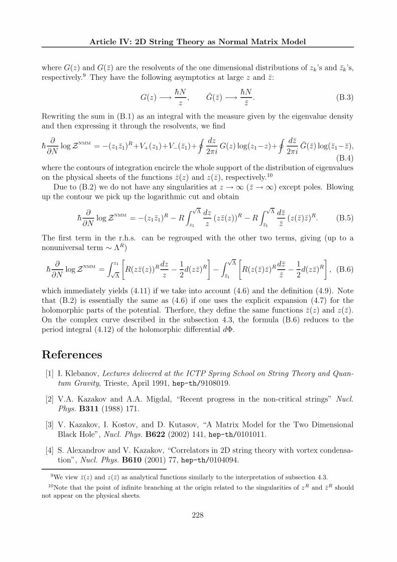
Article IV: 2D String Theory as Normal Matrix Model
where G(z) and G(z) are the resolvents of the one dimensional distributions of zk’s and zk’s,respectively.9 They have the following asymptotics at large z and z:
G(z) −→ hN
z, G(z) −→ hN
z. (B.3)
Rewriting the sum in (B.1) as an integral with the measure given by the eigenvalue densityand then expressing it through the resolvents, we find
h∂
∂NlogZNMM = −(z1z1)
R+V+(z1)+V−(z1)+∮
dz
2πiG(z) log(z1−z)+
∮
dz
2πiG(z) log(z1−z),
(B.4)where the contours of integration encircle the whole support of the distribution of eigenvalueson the physical sheets of the functions z(z) and z(z), respectively.10
Due to (B.2) we do not have any singularities at z → ∞ (z → ∞) except poles. Blowingup the contour we pick up the logarithmic cut and obtain
h∂
∂NlogZNMM = −(z1z1)
R − R∫
√Λ
z1
dz
z(zz(z))R −R
∫
√Λ
z1
dz
z(z(z)z)R. (B.5)
The first term in the r.h.s. can be regrouped with the other two terms, giving (up to anonuniversal term ∼ ΛR)
h∂
∂NlogZNMM =
∫ z1
√Λ
[
R(zz(z))Rdz
z− 1
2d(zz)R
]
−∫
√Λ
z1
[
R(z(z)z)Rdz
z− 1
2d(zz)R
]
, (B.6)
which immediately yields (4.11) if we take into account (4.6) and the definition (4.9). Notethat (B.2) is essentially the same as (4.6) if one uses the explicit expansion (4.7) for theholomorphic parts of the potential. Therfore, they define the same functions z(z) and z(z).On the complex curve described in the subsection 4.3, the formula (B.6) reduces to theperiod integral (4.12) of the holomorphic differential dΦ.
References
[1] I. Klebanov, Lectures delivered at the ICTP Spring School on String Theory and Quan-
tum Gravity, Trieste, April 1991, hep-th/9108019.
[2] V.A. Kazakov and A.A. Migdal, “Recent progress in the non-critical strings” Nucl.
Phys. B311 (1988) 171.
[3] V. Kazakov, I. Kostov, and D. Kutasov, “A Matrix Model for the Two DimensionalBlack Hole”, Nucl. Phys. B622 (2002) 141, hep-th/0101011.
[4] S. Alexandrov and V. Kazakov, “Correlators in 2D string theory with vortex condensa-tion”, Nucl. Phys. B610 (2001) 77, hep-th/0104094.
9We view z(z) and z(z) as analytical functions similarly to the interpretation of subsection 4.3.10Note that the point of infinite branching at the origin related to the singularities of zR and zR should
not appear on the physical sheets.
228

References
[5] S. Alexandrov and V. Kazakov, “Thermodynamics of 2D string theory”, JHEP 0301(2003) 078, hep-th/0210251.
[6] I. Kostov, “String Equation for String Theory on a Circle”, Nucl. Phys. B624 (2002)146, hep-th/0107247.
[7] D. Ghoshal and C. Vafa, “c=1 String as the Topological Theory of the Conifold”, Nucl.
Phys. B453 (1995) 121, hep-th/9506122.
[8] R. Dijkgraaf and C. Vafa, “N = 1 Supersymmetry, Deconstruction and Bosonic GaugeTheories”, hep-th/0302011.
[9] J. Polchinski, “What is string theory”, Lectures presented at the 1994 Les Houches
Summer School “Fluctuating Geometries in Statistical Mechanics and Field Theory”,hep-th/9411028.
[10] A. Jevicki, “Developments in 2D string theory”, hep-th//9309115.
[11] S.Yu. Alexandrov, V.A. Kazakov, and I.K. Kostov, “Time-dependent backgrounds of2D string theory”, Nucl. Phys. B640 (2002) 119, hep-th/0205079.
[12] R.Dijkgraaf, G.Moore, and M.R.Plesser, “The partition function of 2d string theory”,Nucl. Phys. B394 (1993) 356, hep-th/9208031.
[13] K. Takasaki and T. Takebe, “Integrable Hierarchies and Dispersionless Limit”, Rev.
Math. Phys. 7 (1995) 743, hep-th/9405096.
[14] S. Mukhi and C. Vafa, “Two dimensional black-hole as a topological coset model of c=1string theory”, Nucl. Phys. B407 (1993) 667, hep-th/9301083.
[15] C. Imbimbo and S. Mukhi, “The topological matrix model of c=1 String”, Nucl. Phys.
B449 (1995) 553, hep-th/9505127.
[16] I. Kostov, I. Krichever, M. Mineev-Veinstein, P. Wiegmann, and A. Zabrodin, “τ -function for analytic curves”, Random matrices and their applications, MSRI publi-
cations 40 (2001) 285 (Cambridge University Press), hep-th/0005259.
[17] A. Zabrodin, “Dispersionless limit of Hirota equations in some problems of complexanalysis”, Theor. Math. Phys. 129 (2001) 1511; Theor. Math. Phys. 129 (2001) 239,math.CV/0104169.
[18] A. Boyarsky, A. Marshakov, O. Ruchhayskiy, P. Wiegmann, and A. Zabrodin, “Onassociativity equations in dispersionless integrable hierarchies”, Phys. Lett. B515 (2001)483, hep-th/0105260.
[19] P. Wiegmann and A. Zabrodin, “Conformal maps and dispersionless integrable hierar-chies”, Comm. Math. Phys. 213 (2000) 523, hep-th/9909147.
[20] P. Wiegmann and A. Zabrodin, “Large scale correlations in normal and general non-Hermitian matrix ensembles”, hep-th/0210159.
229
Article IV: 2D String Theory as Normal Matrix Model
[21] O. Agam, E. Bettelheim, P. Wiegmann, and A. Zabrodin, “Viscous fingering and ashape of an electronic droplet in the Quantum Hall regime”, Phys. Rev. Lett.88 (2002)236802, cond-mat/0111333.
[22] F. David, “Non-Perturbative Effects in Matrix Models and Vacua of Two DimensionalGravity”, Phys. Lett. B302 (1993) 403, hep-th/9212106.
[23] G. Bonnet, F. David, and B. Eynard, “Breakdown of universality in multi-cut matrixmodels”, J. Phys. A33 (2000) 6739, cond-mat/0003324.
[24] I. K. Kostov, “Conformal Field Theory Techniques in Random Matrix models”,hep-th/9907060.
[25] V. Kazakov and A. Marshakov, “Complex Curve of the Two Matrix Model and itsTau-function”, hep-th/0211236.
[26] R. Dijkgraaf and C. Vafa, “Matrix Models, Topological Strings, and SupersymmetricGauge Theories”, Nucl. Phys. B644 (2002) 3, hep-th/0206255.
[27] R. Dijkgraaf and C. Vafa, “On Geometry and Matrix Models”, Nucl. Phys. B644 (2002)21, hep-th/0207106.
[28] R. Dijkgraaf and C. Vafa, “A Perturbative Window into Non-Perturbative Physics”,hep-th/0208048.
[29] A. Boyarsky and O. Ruchayskiy, “Integrability in SFT and new representation of KPtau-function”, hep-th/0211010.
[30] E. Witten, “Ground Ring of two dimensional string theory”, Nucl. Phys. B373 (1992)187, hep-th/9108004.
[31] M. Adler and P. van Moerbeke, “String-Orthogonal Polynomials, String equations, and2-Toda symmetries”, Commun. Pure Appl. Math. 50 (1997) 241, hep-th/9706182.
230

Article V
Backgrounds of 2D string theory
from matrix model
submitted to Nucl. Phys.


SPHT-t03/058, LPTENS-03/13hep-th/0303190
Backgrounds of 2D string theory from matrixmodel
S. Yu. Alexandrov
Service de Physique Theorique, CNRS - URA 2306, C.E.A. - Saclay,
F-91191 Gif-Sur-Yvette CEDEX, France
Laboratoire de Physique Theorique de l’Ecole Normale Superieure†
24 rue Lhomond, 75231 Paris Cedex 05, France
V.A. Fock Department of Theoretical Physics, St. Petersburg University, Russia
In the Matrix Quantum Mechanical formulation of 2D string theory it is possible to in-troduce arbitrary tachyonic perturbations. In the case when the tachyonic momenta forma lattice, the theory is known to be integrable and, therefore, it can be used to describethe corresponding string theory. We study the backgrounds of string theory obtained fromthese matrix model solutions. They are found to be flat but the perturbations can changethe global structure of the target space. They can lead either to a compactification, or tothe presence of boundaries depending on the choice of boundary conditions. Thus, we arguethat the tachyon perturbations have a dual description in terms of the unperturbed theoryin spacetime with a non-trivial global structure.
†Unite de Recherche du Centre National de la Recherche Scientifique et de l’Ecole Normale Superieureet a l’Universite de Paris-Sud.

Article V: Backgrounds of 2D string theory from matrix model
1 Introduction
The two-dimensional string theory has proven to be a model possessing a very rich structure[1, 2, 3]. It allows to address various questions inaccessible in higher dimensional stringtheories as well as it appears as an equivalent description of topological strings and super-symmetric gauge theories [4, 5, 6]. Perhaps, its main feature is the integrability. Manyproblems formulated in its framework, such as calculation of S-matrix, were found to beexactly solvable.
However, this integrability is hidden in the usual CFT formulation and becomes explicitonly when one uses a matrix model description of string theory. In this case the model, onehas to consider, is the Matrix Quantum Mechanics (MQM) [7]. It was successfully used todescribe 2D string theory in the simplest linear dilaton background as well as to incorporateperturbations. In two dimensions there are basically two types of possible perturbations:tachyon and winding modes. The former always present in the theory as momentum modesof a massless field which, following tradition, is called “tachyon”. The latter appear whenone considers Euclidean theory compactified on a time circle.
There are two ways to change the background of string theory: either to consider stringspropagating in a non-trivial target space or to introduce the perturbations mentioned above.In the first case one arrives at a complicated sigma-model. Not many examples are knownwhen such a model turns out to be solvable. Besides, it is extremely difficult to constructa matrix model realization of a general sigma-model since not much known about matrixoperators explicitly perturbing the metric of the target space. Thus, we lose the possibilityto use the powerful matrix model machinery to tackle our problems.
On the other hand, following the second way, we find that the integrability of the theoryin the trivial background is preserved by the perturbations. Namely, when we restrict ourattention only to windings or to tachyons with discrete momenta, they are described byToda integrable hierarchy [8, 9, 10]. Therefore, the backgrounds of string theory obtainedby these perturbations represent a good laboratory for investigation of different problems.
One of the such interesting problems is the black hole thermodynamics. As it is wellknown, 2D string theory possesses an exact background which incorporates the black holesingularity [11, 12]. From the target space point of view, it is described just by one of thedilaton models, the so-called CHGS model [13]. Its thermodynamical properties have beenextensively studied (see, for example, the review on dilaton models [14]). However, to achievethe microscopical statistical description, one should deal with the full string theory so thatone has to obtain the complete solution of the corresponding sigma-model.
Fortunately, there exists an alternative description of string theory in this background.It has been conjectured that the black hole background can be created also by introductionof the winding modes [15]. Moreover, a matrix model incorporating these perturbationshas been proposed [9]. Thus, we get a possibility to describe dynamics of string theory innon-trivial backgrounds using the usual perturbations of MQM.
In this paper we consider tachyon perturbations of 2D string theory which are T-dual toperturbations by winding modes. We saw that the latter are supposed to create curvatureof the target space. Do tachyon perturbations can also change the structure of the targetspace? The paper is devoted to addressing this question.
First of all, we explain why we study tachyon and not winding perturbations, whereas
234

§2 Tachyon and winding modes in 2D Euclidean string theory
these are the windings that have the most interesting physical applications like the physicsof black holes. The main reason is that it is much easier to study the tachyon modes fromthe MQM point of view. In this case we have a powerful description in terms of free fermionson the one hand [16] and the Das–Jevicki collective field theory on the other [17]. The latterhas a direct target space interpretation what allows to identify matrix model quantitieswith characteristics of the string background. However, this description is absent when thewinding modes are included what is possibly related to the absence of a local target spaceinterpretation of windings.
Tachyon modes do have such local interpretation and, therefore, the background, whichthey create, is characterized simply by a (time-dependent) condensate of these modes. How-ever, we are looking for another description which would be dual to the one with the tachyoncondensate. We expect it to be similar to the dual description of the winding perturbations,that is it should replace the time-dependent tachyon condensate by a change of the structureof the target space.
As one of justifications of why such dual description should exist, we mention that ithas been shown that the tachyon perturbations lead to a finite temperature as if we had ablack hole [18]. In fact, to give rise a temperature, it is not necessary for the target space tocontain a black hole singularity. The thermal description can arise in very different situationsincluding flat spacetimes, but in any case it should be different from the usual Minkowskispace [19].
In this paper we show that comparison of the Das–Jevicki collective theory with thelow-energy effective action for the string background leads to the picture we sketched above.Instead of the tachyon condensate we get the target space with a non-trivial global structure.Non-triviality can appear either as boundaries or as a compactification. Locally spacetimeremains the same as it was before the perturbation.
The paper is organized as follows. In the next section we briefly review 2D string theoryin the CFT formulation. In section 3 the Das–Jevicki collective field theory for the singletsector of MQM is analyzed. We derive an effective action for the quantum correction to theeigenvalue density of MQM. In section 4 this correction and its action are identified with thetachyon field of string theory and the low-energy effective action for the string background,correspondingly. The identification imposes a condition which leaves us with the lineardilaton background. However, there is still a freedom to have a non-trivial global structurewhich is investigated in section 5. The case of the simplest Sine–Liouville perturbation isconsidered in detail.
2 Tachyon and winding modes in 2D Euclidean string
theory
2D string theory is defined by the Polyakov action
SP =1
4π
∫
d2σ√h[hab∂aX∂bX + µ], (2.1)
where the bosonic field X(σ) describes the embedding of the string into the Euclidean timedimension and hab is a world sheet metric. In the conformal gauge hab = eφ(σ)hab, where
235

Article V: Backgrounds of 2D string theory from matrix model
hab is a background metric, the conformal mode φ becomes dynamical due to the conformalanomaly and the world-sheet CFT action takes the familiar Liouville form
S0 =1
4π
∫
d2σ [(∂X)2 + (∂φ)2 − 2Rφ+ µe−2φ + ghosts]. (2.2)
This action is known to describe the unperturbed linear dilaton string background corre-sponding to the flat 2D target space parameterized by the coordinates (X, φ) [20].
In two dimensions string theory possesses only one field-theoretic degree of freedom,which is called “tachyon” since it corresponds to the tachyon mode of the bosonic string in26 dimensions. However, in the present case it is massless. The vertex operators for thetachyons of momentum p are written as
Vp =Γ(|p|)
Γ(−|p|)∫
d2σ eipXe(|p|−2)φ. (2.3)
If we consider the Euclidean theory compactified to a time circle of radius R, the momentumis allowed to take only discrete values pn = n/R, n ∈ Z. In this case there are also windingmodes of the string around the compactified dimension which also have a representation inthe CFT (2.2) as vortex operators Vq.
Both tachyons and windings can be used to perturb the simplest theory (2.2)
S = S0 +∑
n6=0
(tnVn + tnVn). (2.4)
How do these perturbations look from the target space point of view? The presence of non-vanishing couplings tn (together with the cosmological constant µ) means that we considera string propagation in the background with a non-trivial vacuum expectation value of thetachyon. In particular, the introduction of momentum modes makes it to be time-dependent.On the other hand, the winding modes, which are defined in terms of the T-dual world sheetfield X = XR − XL, where XR and XL are the right and left-moving components of theinitial field X(σ), have no obvious interpretation in terms of massless background fields.Since windings are related to global properties of strings, they should correspond to somenon-local quantities in the low-energy limit. Their condensation can result in change of thebackground we started with.
A particular proposal for the structure of the resulting background has been made forthe simplest case of t±1 6= 0 [15]. The CFT with the lowest winding perturbation has beenconjectured to be dual to the WZW SL(2,R)/U(1) sigma-model, which describes the 2Dstring theory on the black hole background [11, 12, 21]. In [10] it was suggested that anyperturbation of type (2.4) should have a dual description as string theory in some non-trivialbackground, which is determined by the two sets of couplings tn and tn. Thus, not only forwinding, but also for tachyon perturbations we expect to find such a description.
Note, that the two sets of perturbations are related by T-duality on the world sheet [1].However, this does not mean that the corresponding string backgrounds should be the same.This is because the momentum and winding modes have different target space interpretationsand it is not clear how to carry over this T-duality from the world sheet to the target space.
236

§3 Das–Jevicki collective field theory
3 Das–Jevicki collective field theory
The 2D string theory can be described using Matrix Quantum Mechanics in the double scal-ing limit (for review see[1]). The matrix model Lagrangian corresponding to the unperturbedCFT (2.2) is
L = Tr(
1
2M2 − u(M)
)
, (3.1)
where u(M) = − 12M2 is the inverse oscillator potential. It is known also how to introduce
tachyons and windings into this model [10, 22, 23, 9]. In the following we restrict ourselvesto the tachyon perturbations. In this case it is enough to consider only the singlet sectorof MQM, where the wave function is a completely antisymmetric function of the matrixeigenvalues xi. Due to this the system has an equivalent description in terms of free fermionsin the potential u(M).
The fermionic description is very powerful and allows to calculate many interesting quan-tities in the theory. However, to make contact with the target space description of stringtheory, another representation has proven to be quite useful. It is obtained by a bosonizationprocedure and leads to a collective field theory developed by Das and Jevicki [17, 3]. Therole of the collective field is played by the density of matrix eigenvalues
ϕ(x, t) = Tr δ (x−M(t)) . (3.2)
If to introduce the conjugated field Π(x) such that
ϕ(x),Π(y) = δ(x, y), (3.3)
the effective action for the collective theory is written as
Scoll =∫
dt [∫
dx (Π∂tϕ) −Hcoll] , (3.4)
where Hcoll =∫
dx(
12ϕ(∂xΠ)2 + π2
6ϕ3 + (u(x) + µ)ϕ
)
and we added the chemical potential µ to the action. The classical equations of motion read
−∂xΠ =1
ϕ
∫
dx∂tϕ, (3.5)
−∂tΠ =1
2(∂xΠ)2 +
π2
2ϕ2 + (u(x) + µ). (3.6)
Due to the first equation one can exclude the momenta and pass to the Lagrangian form ofthe action
Scoll =∫
dt∫
dx
(
1
2ϕ
(∫
dx∂tϕ)2
− π2
6ϕ3 − (u(x) + µ)ϕ
)
(3.7)
with the following equation for the classical field
∂t
(∫
dx∂tϕ
ϕ
)
=1
2∂x
(∫
dx∂tϕ
ϕ
)2
+π2
2∂xϕ
2 + ∂xu(x). (3.8)
237

Article V: Backgrounds of 2D string theory from matrix model
Let us consider a function 1πϕ0(x, t), which is a solution of the classical equation of motion
(3.8). We expand the collective field around the background given by this solution
ϕ(x, t) =1
πϕ0(x, t) +
1√π∂xη(x, t). (3.9)
The action takes the formScoll = S(0) + S(1) + S(2) + · · · , (3.10)
where S(0) is a constant, S(1) vanishes due to the equation (3.8), and S(2) is given by
S(2) =1
2
∫
dt∫
dx
ϕ0
(∂tη)2 − 2
∫
dx∂tϕ0
ϕ0∂tη∂xη −
ϕ20 −
(∫
dx∂tϕ0
ϕ0
)2
(∂xη)2
. (3.11)
We want to use the quadratic part of the action to extract information about the back-ground of string theory corresponding to the solution ϕ0(x, t). For that we will identify thequantum correction η with the tachyon field and interpret (3.11) as the kinetic term for thetachyon in the low-energy string effective action. Therefore, we will need the properties ofthe matrix standing in front of derivatives of η. The crucial property is that for any ϕ0 itsdeterminant is equal to −1. As a result, the action can be represented in the following form
S(2) = −1
2
∫
dt∫
dx√−ggµν∂µη∂νη. (3.12)
In a more general case we would have to introduce a dilaton dependent factor coupled withthe kinetic term.
The action (3.12) is conformal invariant. Therefore, one can always choose coordinateswhere the metric takes the usual Minkowski form ηµν = diag(−1, 1). Unfortunately, we donot know the explicit form of this transformation for arbitrary solution ϕ0. Note, however,that one can bring the metric to another standard form which is of the Schwarzschild type.Indeed, it is easy to check that if one changes the x coordinate to
y(x, t) =∫
ϕ0(x, t)dx, (3.13)
the metric becomes
gµν =(−ϕ2
0 00 ϕ−2
0
)
. (3.14)
4 Low-energy effective action and background of 2D
string theory
Now we turn to the string theory side of the problem. In a general background the stringtheory is defined by the following σ-model action
Sσ =1
4πα′
∫
d2σ√h[
Gµν(X)hab∂aXµ∂bX
ν + α′RΦ(X) + T (X)]
, (4.1)
where X(σ) is a two-dimensional field on the world sheet. As it is well known the conditionthat the conformal invariance of this theory is unbroken reduces to some equations on the
238

§4 Low-energy effective action and background of 2D string theory
background fields: target space metric Gµν , dilaton Φ and tachyon T . These equations canbe obtained from the effective action which in the leading order in α′ is given by [24]
Seff =1
2
∫
d2X√−Ge−2Φ
[
16
α′ +R + 4(∇Φ)2 − (∇T )2 +4
α′T2]
. (4.2)
Here the covariant derivative ∇µ is defined with respect to the metric Gµν and R is itscurvature. The first term comes from the central charge and in D dimensions looks as2(26−D)
3α′ disappearing in the critical case. The equations of motion following from the action(4.2) are equivalent to
βGµν = Rµν + 2∇µ∇νΦ −∇µT∇νT = 0,
4
α′βΦ = −16
α′ −R + 4(∇Φ)2 − 4∇2Φ + (∇T )2 − 4
α′T2 = 0, (4.3)
βT = −2∇2T + 4∇Φ · ∇T − 8
α′T = 0.
Let us concentrate on the tachyonic part of the action (4.2). We want to relate it tothe action (3.12) for the collective theory obtained form Matrix Quantum Mechanics. Inparticular, the tachyon field T and quantum fluctuation of density η should be correctlyidentified with each other. We see that the main difference between (4.2) and (3.12) is thepresence of the dilaton dependent factor e−2Φ. To remove this factor, we redefine the tachyonas T = eΦη. Then the part of the action quadratic in the tachyon field reads
Stach = −1
2
∫
d2X√−G
[
(∇η)2 +m2ηη
2]
, (4.4)
where
m2η = (∇Φ)2 −∇2Φ − 4α′−1. (4.5)
We denoted the new tachyon by the same letter as the matrix model field since they should beidentical. However, comparing two actions (4.4) and (3.12), we see that for this identificationto be true, one must require the vanishing of the tachyonic mass
m2η = 0. (4.6)
This equation plays the role of an additional condition for the equations of motion (4.3) andallows to select the unique solution. It is easy to check that the linear dilaton background
Gµν = ηµν, Φ = − 2√α′X
1, η = 0 (4.7)
satisfies all these equations. Besides, we argue that it is the unique solution of the equations(4.3) and (4.6). It means that for any solution of MQM restricted to the singlet sector wealways get the simplest linear dilaton background. Since the theory (4.2) is a model of two-dimensional dilaton gravity with non-minimal coupled scalar field, it is not exactly solvable[14]. Therefore, we are not able to prove our statement rigorously. However, in Appendix A
239
Article V: Backgrounds of 2D string theory from matrix model
we show that there are no solutions which can be represented as an expansion around thelinear dilaton background (4.7).1
Thus, any tachyon perturbation can not modify the local structure of spacetime. How-ever, the found solution does not forbid modifications of the global structure. There are, inprinciple, two possibilities to change it. Either something can happen with the topology, forexample, a spontaneous compactification, or there can appear boundaries. We argue thatjust these possibilities are indeed realized in our case.
To understand why this can happen, note that in the initial coordinates (t, x) of MQMthe metric is non-trivial, although flat. We can represent it as
Gµν = e2ρgµν, (4.8)
where gµν is the matrix coupled with the derivatives of η in (3.11), whose determinantequals −1. It takes the usual form ηµν only after a coordinate transformation. Under thistransformation, the image of the (t, x)-plane is, in general, not the whole plane, but some itssubspace. Depending on boundary conditions, it will give rise either to a compactification,or to the appearance of boundaries.
5 Target space of string theory with integrable tachyon
perturbations
In this section we analyze the structure of the target space of 2D string theory in thepresence of tachyon perturbations with discrete momenta. Such perturbations correspondto the admissible perturbations of the Euclidean theory described in section 2. Nevertheless,our analysis is carried out in spacetime of the Minkowskian signature.
The case, we consider here, was shown to be exactly integrable and described by TodaLattice hierarchy [10]. Therefore, it is possible to find explicitly the classical solution ϕ0,playing the role of the background field in the Das–Jevicki collective theory. Moreover, as wewill show, the integrability manifests itself at the next steps of the derivation, what allowsto complete the analysis of this case.
5.1 Background field from matrix model solution
First, we show how the classical solution ϕ0 determining the string background can beextracted from MQM. As it was noted, it represents the density of eigenvalues. The latteris most easily found from the exact form of the Fermi sea formed by fermions of the MQMsinglet sector. To see how this works, let us introduce the left and right moving chiral fields
1Of course, this result is valid only for the equations of motion obtained in the leading order in α′. Forexample, the background described by the CFT (2.2) or even (2.4) with tn = 0 corresponds to the lineardilaton background with a non-vanishing tachyon field. Such background does not satisfy the equations(4.3). However, it was suggested that it satisfies the exact equations which include all corrections in α′ [2].We are interested in the existence of a dual description where the non-vanishing tachyon vacuum transformsinto expectation values of other fields. Our results show that the curvature of the target space and thedilaton can not be changed in the leading order in α′.
240

§5 Target space of string theory with integrable tachyon perturbations
[3]:p±(x, t) = ∂xΠ ± πϕ(x, t). (5.1)
They have the following Poisson brackets
p±(x), p±(y) = ∓2π∂xδ(x− y) (5.2)
and bring the Hamiltonian to the form
Hcoll =∫
dx
2π
(
1
6(p3
+ − p3−) + (u(x) + µ)(p+ − p−)
)
. (5.3)
Using (5.2), it is easy to show that they should satisfy the Hopf equation
∂tp± + p±∂xp± + ∂xu(x) = 0. (5.4)
This equation is of integrable type and much easier to solve than eq. (3.8). The keyobservation, which establishes the contact with MQM, is that in the quasiclassical limitp±(x, t) determine the upper and lower boundaries of the Fermi sea in the phase space.Then the density is given by their difference what agrees with the definition (5.1).
For general integrable tachyon perturbations, the solution for the profile of the Fermi seahas been found in [10]. If we introduce the sources for tachyons with momenta pk = k/R,k = 1, . . . , n, it can be represented in the following parametric form
p(ω, t) =n∑
k=0ak sinh
[(
1 − kR
)
ω + kRt + αk
]
,
x(ω, t) =n∑
k=0ak cosh
[(
1 − kR
)
ω + kRt + αk
]
.(5.5)
Here ak are coefficients which can be found in terms of the coupling constants tk of thetachyon operators and the chemical potential µ which fixes the Fermi level. Actually, theydepend only on µ and the products λ2
k = tkt−k. Instead, the “phases” αk are determined byratios of the coupling constants. (Two of them can be excluded by constant shifts of ω andt.) It is easy to check that p(x, t) indeed satisfies (5.4) with u(x) = − 1
2x2.
To get from this solution ϕ0, note that p(x) is a two-valued function so that p±(x) canbe identified with its two branches. As functions of ω they appear as follows. Let us definea ”mirror” parameter ω(ω, t) such that (see fig. 1)
x(ω(ω, t), t) = x(ω, t), ω 6= ω. (5.6)
Then p+ can be identified with p and p− with p(ω(ω, t), t). The solution for the backgroundfield is given again in the parametric form
ϕ0(ω, t) =1
2(p(ω, t) − p(ω, t)), (5.7)
where we denoted p(ω, t) = p(ω(ω, t), t) and ω is related to x by eq. (5.5). Due to (3.5),(5.1) and (5.7), the effective action (3.11) can now be rewritten as
S(2) =∫
dt∫
dx
p− p
[
(∂tη)2 + (p+ p)∂tη∂xη + pp(∂xη)
2]
. (5.8)
241

Article V: Backgrounds of 2D string theory from matrix model
(ω, t)ω∼
sing(t)ω
(ω, t)p
ω
(ω, t)ϕ0
(ω, t)p∼
x
p
Fig. V.1: The Fermi sea of the perturbed MQM. Its boundary is defined by a two-valuedfunction with two branches parameterized by p(ω, t) and p(ω, t). The background field ϕ0
coincides with the width of the Fermi sea.
5.2 Flat coordinates
We know from section 4 that any background described by the Das-Jevicki effective actionleads to the flat target space metric. However, as we discussed above, the global structureof the target space can differ from that of the usual Minkowski space. To find whether thisis the case, one should investigate the coordinate transformation mapping the target spacemetric into the standard form ηµν .
In general, it is quite a difficult problem to find such a map explicitly. Remarkably, inour case given by the solution (5.5), this task can be accomplished. Indeed, we show inAppendix B that the change of coordinates from (t, x) to (τ, q) with
τ = t− ω + ω
2, q =
ω − ω
2(5.9)
brings the action (5.8) to the standard form
S(2) = ±1
2
∫
dτ∫
dq[
(∂τη)2 − (∂qη)
2]
, (5.10)
where the sign is determined by the sign of the Jacobian of the coordinate transformation(5.9). The Jacobian is defined by the function D in (B.2) and can be represented in the form
2D =2(p− xt)(p− xt)
p− p, (5.11)
where xt ≡ ∂tx(ω, t) and xt ≡ xt(ω, t) given explicitly in (B.4).The zeros of the Jacobian show where the map (5.9) is degenerate. All multipliers in (5.11)
vanish at the line defined by the condition ω(ω, t) = ω or ∂x/∂ω = 0, which corresponds tothe most left point of the Fermi sea where two branches of p(x) meet each other (see fig. 1).In terms of the flat coordinates (5.9), this line is given in the following parametric form
τ = t− ωsing(t), q = 0, (5.12)
242

§5 Target space of string theory with integrable tachyon perturbations
where ωsing(t) is a solution of the above condition. Also it defines the limiting value ofthe coordinate x, which should always be larger than xsing(t) = x(ωsing(t), t). However,the spacetime can be analytically continued through this line. This analytical continuationcorresponds to that in all integrals x should run from ∞ to xsing and return back withsimultaneous interchanging the roles of p and p. This shows that it is more natural toconsider the plane of (t, ω) as the starting point rather than (t, x). The former is a two-sheet cover of the physical region of the latter. ω appears as a parameter along fermionictrajectories and it should not be restricted to a half-line. Thus, we incorporate the wholescattering picture and glue two copies of the resulting flat spacetime together along the line(5.12).
Unfortunately, there is an ambiguity in the choice of coordinates where the action hasthe form (5.10). Any conformal change of variables (5.9)
(τ, q) −→ (u(t− ω), v(t− ω)) (5.13)
leaves the action unchanged. Due to this we can find the form of the resulting spacetimeonly up to the conformal map. However, one can reduce the ambiguity imposing someconditions on the map (5.13). First of all, it should be well defined on the subspace whichis the image of the (t, ω)-plane under the map (5.9), that is the functions u and v shouldnot have singularities there. The next condition is the triviality of (5.13) in the absence ofperturbations since in this limit (5.9) reduces to the well known transformation giving theflat Minkowski space [3]. Besides, we would like to retain the symmetry (t, ω) ↔ (−t,−ω)which is explicit when there are no phases αk in (5.5). It reflects the fact the our spacetimeis glued from two identical copies (see discussion in the previous paragraph). This leads tothe condition that u and v are odd functions.
As a byproduct of our analysis we obtain also the conformal factor e2ρ appearing in (4.8).It should be found, in principle, from the condition of vanishing curvature for the metric Gµν.Instead, we get it as the Jacobian of the transformation to the coordinates where Gµν = ηµν .If u and v from (5.13) are such coordinates, than dtdx
√−G = dudv and, since
√−G = e2ρ,
we conclude from (5.11) that
e2ρ =p− p
2(p− xt)(p− xt)u′v′. (5.14)
The conformal factor becomes singular on the line (5.12) discussed above. However, this isonly a coordinate singularity since it disappears after our coordinate transformation.
5.3 Structure of the target space
In this subsection we investigate the concrete form of the target space which is obtained asthe image under the coordinate transformation trivializing the metric. From the previoussubsection it follows that this transformation is a superposition of the map (5.9) and aconformal change of coordinates (5.13). Since the latter remains unknown, we will analyzeonly the image of the map (5.9). It will be sufficient to get a general picture becauseconformal transformations do not change the causal structure of spacetime.
We restrict our analysis to the case of the simplest non-trivial perturbation with n = 1in (5.5). It corresponds to the conformal Sine-Liouville theory. At R = 2/3 this theory is
243
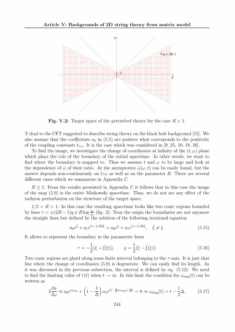
Article V: Backgrounds of 2D string theory from matrix model
+,+,+,+,+,+,+,+,+,+,+,+,+,+,+,+,+,+,+,+,+,+,+,+,+,+,+,+,+,+,+,+,+,+,+,+,+,+,+,+,+,+,+,+,+,+,+,+,++,+,+,+,+,+,+,+,+,+,+,+,+,+,+,+,+,+,+,+,+,+,+,+,+,+,+,+,+,+,+,+,+,+,+,+,+,+,+,+,+,+,+,+,+,+,+,+,++,+,+,+,+,+,+,+,+,+,+,+,+,+,+,+,+,+,+,+,+,+,+,+,+,+,+,+,+,+,+,+,+,+,+,+,+,+,+,+,+,+,+,+,+,+,+,+,++,+,+,+,+,+,+,+,+,+,+,+,+,+,+,+,+,+,+,+,+,+,+,+,+,+,+,+,+,+,+,+,+,+,+,+,+,+,+,+,+,+,+,+,+,+,+,+,++,+,+,+,+,+,+,+,+,+,+,+,+,+,+,+,+,+,+,+,+,+,+,+,+,+,+,+,+,+,+,+,+,+,+,+,+,+,+,+,+,+,+,+,+,+,+,+,++,+,+,+,+,+,+,+,+,+,+,+,+,+,+,+,+,+,+,+,+,+,+,+,+,+,+,+,+,+,+,+,+,+,+,+,+,+,+,+,+,+,+,+,+,+,+,+,++,+,+,+,+,+,+,+,+,+,+,+,+,+,+,+,+,+,+,+,+,+,+,+,+,+,+,+,+,+,+,+,+,+,+,+,+,+,+,+,+,+,+,+,+,+,+,+,++,+,+,+,+,+,+,+,+,+,+,+,+,+,+,+,+,+,+,+,+,+,+,+,+,+,+,+,+,+,+,+,+,+,+,+,+,+,+,+,+,+,+,+,+,+,+,+,++,+,+,+,+,+,+,+,+,+,+,+,+,+,+,+,+,+,+,+,+,+,+,+,+,+,+,+,+,+,+,+,+,+,+,+,+,+,+,+,+,+,+,+,+,+,+,+,++,+,+,+,+,+,+,+,+,+,+,+,+,+,+,+,+,+,+,+,+,+,+,+,+,+,+,+,+,+,+,+,+,+,+,+,+,+,+,+,+,+,+,+,+,+,+,+,++,+,+,+,+,+,+,+,+,+,+,+,+,+,+,+,+,+,+,+,+,+,+,+,+,+,+,+,+,+,+,+,+,+,+,+,+,+,+,+,+,+,+,+,+,+,+,+,++,+,+,+,+,+,+,+,+,+,+,+,+,+,+,+,+,+,+,+,+,+,+,+,+,+,+,+,+,+,+,+,+,+,+,+,+,+,+,+,+,+,+,+,+,+,+,+,++,+,+,+,+,+,+,+,+,+,+,+,+,+,+,+,+,+,+,+,+,+,+,+,+,+,+,+,+,+,+,+,+,+,+,+,+,+,+,+,+,+,+,+,+,+,+,+,++,+,+,+,+,+,+,+,+,+,+,+,+,+,+,+,+,+,+,+,+,+,+,+,+,+,+,+,+,+,+,+,+,+,+,+,+,+,+,+,+,+,+,+,+,+,+,+,++,+,+,+,+,+,+,+,+,+,+,+,+,+,+,+,+,+,+,+,+,+,+,+,+,+,+,+,+,+,+,+,+,+,+,+,+,+,+,+,+,+,+,+,+,+,+,+,++,+,+,+,+,+,+,+,+,+,+,+,+,+,+,+,+,+,+,+,+,+,+,+,+,+,+,+,+,+,+,+,+,+,+,+,+,+,+,+,+,+,+,+,+,+,+,+,++,+,+,+,+,+,+,+,+,+,+,+,+,+,+,+,+,+,+,+,+,+,+,+,+,+,+,+,+,+,+,+,+,+,+,+,+,+,+,+,+,+,+,+,+,+,+,+,++,+,+,+,+,+,+,+,+,+,+,+,+,+,+,+,+,+,+,+,+,+,+,+,+,+,+,+,+,+,+,+,+,+,+,+,+,+,+,+,+,+,+,+,+,+,+,+,++,+,+,+,+,+,+,+,+,+,+,+,+,+,+,+,+,+,+,+,+,+,+,+,+,+,+,+,+,+,+,+,+,+,+,+,+,+,+,+,+,+,+,+,+,+,+,+,++,+,+,+,+,+,+,+,+,+,+,+,+,+,+,+,+,+,+,+,+,+,+,+,+,+,+,+,+,+,+,+,+,+,+,+,+,+,+,+,+,+,+,+,+,+,+,+,++,+,+,+,+,+,+,+,+,+,+,+,+,+,+,+,+,+,+,+,+,+,+,+,+,+,+,+,+,+,+,+,+,+,+,+,+,+,+,+,+,+,+,+,+,+,+,+,++,+,+,+,+,+,+,+,+,+,+,+,+,+,+,+,+,+,+,+,+,+,+,+,+,+,+,+,+,+,+,+,+,+,+,+,+,+,+,+,+,+,+,+,+,+,+,+,++,+,+,+,+,+,+,+,+,+,+,+,+,+,+,+,+,+,+,+,+,+,+,+,+,+,+,+,+,+,+,+,+,+,+,+,+,+,+,+,+,+,+,+,+,+,+,+,++,+,+,+,+,+,+,+,+,+,+,+,+,+,+,+,+,+,+,+,+,+,+,+,+,+,+,+,+,+,+,+,+,+,+,+,+,+,+,+,+,+,+,+,+,+,+,+,++,+,+,+,+,+,+,+,+,+,+,+,+,+,+,+,+,+,+,+,+,+,+,+,+,+,+,+,+,+,+,+,+,+,+,+,+,+,+,+,+,+,+,+,+,+,+,+,++,+,+,+,+,+,+,+,+,+,+,+,+,+,+,+,+,+,+,+,+,+,+,+,+,+,+,+,+,+,+,+,+,+,+,+,+,+,+,+,+,+,+,+,+,+,+,+,+
-,-,-,-,-,-,-,-,-,-,-,-,-,-,-,-,-,-,-,-,-,-,-,-,-,-,-,-,-,-,-,-,-,-,-,-,-,-,-,-,-,-,-,-,-,-,-,-,--,-,-,-,-,-,-,-,-,-,-,-,-,-,-,-,-,-,-,-,-,-,-,-,-,-,-,-,-,-,-,-,-,-,-,-,-,-,-,-,-,-,-,-,-,-,-,-,--,-,-,-,-,-,-,-,-,-,-,-,-,-,-,-,-,-,-,-,-,-,-,-,-,-,-,-,-,-,-,-,-,-,-,-,-,-,-,-,-,-,-,-,-,-,-,-,--,-,-,-,-,-,-,-,-,-,-,-,-,-,-,-,-,-,-,-,-,-,-,-,-,-,-,-,-,-,-,-,-,-,-,-,-,-,-,-,-,-,-,-,-,-,-,-,--,-,-,-,-,-,-,-,-,-,-,-,-,-,-,-,-,-,-,-,-,-,-,-,-,-,-,-,-,-,-,-,-,-,-,-,-,-,-,-,-,-,-,-,-,-,-,-,--,-,-,-,-,-,-,-,-,-,-,-,-,-,-,-,-,-,-,-,-,-,-,-,-,-,-,-,-,-,-,-,-,-,-,-,-,-,-,-,-,-,-,-,-,-,-,-,--,-,-,-,-,-,-,-,-,-,-,-,-,-,-,-,-,-,-,-,-,-,-,-,-,-,-,-,-,-,-,-,-,-,-,-,-,-,-,-,-,-,-,-,-,-,-,-,--,-,-,-,-,-,-,-,-,-,-,-,-,-,-,-,-,-,-,-,-,-,-,-,-,-,-,-,-,-,-,-,-,-,-,-,-,-,-,-,-,-,-,-,-,-,-,-,--,-,-,-,-,-,-,-,-,-,-,-,-,-,-,-,-,-,-,-,-,-,-,-,-,-,-,-,-,-,-,-,-,-,-,-,-,-,-,-,-,-,-,-,-,-,-,-,--,-,-,-,-,-,-,-,-,-,-,-,-,-,-,-,-,-,-,-,-,-,-,-,-,-,-,-,-,-,-,-,-,-,-,-,-,-,-,-,-,-,-,-,-,-,-,-,--,-,-,-,-,-,-,-,-,-,-,-,-,-,-,-,-,-,-,-,-,-,-,-,-,-,-,-,-,-,-,-,-,-,-,-,-,-,-,-,-,-,-,-,-,-,-,-,--,-,-,-,-,-,-,-,-,-,-,-,-,-,-,-,-,-,-,-,-,-,-,-,-,-,-,-,-,-,-,-,-,-,-,-,-,-,-,-,-,-,-,-,-,-,-,-,--,-,-,-,-,-,-,-,-,-,-,-,-,-,-,-,-,-,-,-,-,-,-,-,-,-,-,-,-,-,-,-,-,-,-,-,-,-,-,-,-,-,-,-,-,-,-,-,--,-,-,-,-,-,-,-,-,-,-,-,-,-,-,-,-,-,-,-,-,-,-,-,-,-,-,-,-,-,-,-,-,-,-,-,-,-,-,-,-,-,-,-,-,-,-,-,--,-,-,-,-,-,-,-,-,-,-,-,-,-,-,-,-,-,-,-,-,-,-,-,-,-,-,-,-,-,-,-,-,-,-,-,-,-,-,-,-,-,-,-,-,-,-,-,--,-,-,-,-,-,-,-,-,-,-,-,-,-,-,-,-,-,-,-,-,-,-,-,-,-,-,-,-,-,-,-,-,-,-,-,-,-,-,-,-,-,-,-,-,-,-,-,--,-,-,-,-,-,-,-,-,-,-,-,-,-,-,-,-,-,-,-,-,-,-,-,-,-,-,-,-,-,-,-,-,-,-,-,-,-,-,-,-,-,-,-,-,-,-,-,--,-,-,-,-,-,-,-,-,-,-,-,-,-,-,-,-,-,-,-,-,-,-,-,-,-,-,-,-,-,-,-,-,-,-,-,-,-,-,-,-,-,-,-,-,-,-,-,--,-,-,-,-,-,-,-,-,-,-,-,-,-,-,-,-,-,-,-,-,-,-,-,-,-,-,-,-,-,-,-,-,-,-,-,-,-,-,-,-,-,-,-,-,-,-,-,--,-,-,-,-,-,-,-,-,-,-,-,-,-,-,-,-,-,-,-,-,-,-,-,-,-,-,-,-,-,-,-,-,-,-,-,-,-,-,-,-,-,-,-,-,-,-,-,--,-,-,-,-,-,-,-,-,-,-,-,-,-,-,-,-,-,-,-,-,-,-,-,-,-,-,-,-,-,-,-,-,-,-,-,-,-,-,-,-,-,-,-,-,-,-,-,--,-,-,-,-,-,-,-,-,-,-,-,-,-,-,-,-,-,-,-,-,-,-,-,-,-,-,-,-,-,-,-,-,-,-,-,-,-,-,-,-,-,-,-,-,-,-,-,--,-,-,-,-,-,-,-,-,-,-,-,-,-,-,-,-,-,-,-,-,-,-,-,-,-,-,-,-,-,-,-,-,-,-,-,-,-,-,-,-,-,-,-,-,-,-,-,--,-,-,-,-,-,-,-,-,-,-,-,-,-,-,-,-,-,-,-,-,-,-,-,-,-,-,-,-,-,-,-,-,-,-,-,-,-,-,-,-,-,-,-,-,-,-,-,--,-,-,-,-,-,-,-,-,-,-,-,-,-,-,-,-,-,-,-,-,-,-,-,-,-,-,-,-,-,-,-,-,-,-,-,-,-,-,-,-,-,-,-,-,-,-,-,--,-,-,-,-,-,-,-,-,-,-,-,-,-,-,-,-,-,-,-,-,-,-,-,-,-,-,-,-,-,-,-,-,-,-,-,-,-,-,-,-,-,-,-,-,-,-,-,-
q∆
= 2R−1/qτ
τ
Fig. V.2: Target space of the perturbed theory for the case R < 1.
T-dual to the CFT suggested to describe string theory on the black hole background [15]. Wealso assume that the coefficients ak in (5.5) are positive what corresponds to the positivityof the coupling constants t±1. It is the case which was considered in [9, 25, 10, 18, 26].
To find the image, we investigate the change of coordinates at infinity of the (t, ω) planewhich plays the role of the boundary of the initial spacetime. In other words, we want tofind where the boundary is mapped to. Thus we assume t and ω to be large and look atthe dependence of ω of their ratio. At the asymptotics ω(ω, t) can be easily found, but theanswer depends non-continuously on t/ω as well as on the parameter R. There are severaldifferent cases which we summarize in Appendix C.
R ≥ 1: From the results presented in Appendix C it follows that in this case the imageof the map (5.9) is the entire Minkowski spacetime. Thus, we do not see any effect of thetachyon perturbation on the structure of the target space.
1/2 < R < 1: In this case the resulting spacetime looks like two conic regions boundedby lines τ = ±(2R− 1)q±R log a0
a1(fig. 2). Near the origin the boundaries are not anymore
the straight lines but defined by the solution of the following irrational equation
a0eξ + a1e
(1−1/R)ξ = a0eξ + a1e
(1−1/R)ξ , ξ 6= ξ. (5.15)
It allows to represent the boundary in the parametric form
τ = −1
2(ξ + ξ(ξ)), q =
1
2(ξ − ξ(ξ)). (5.16)
Two conic regions are glued along some finite interval belonging to the τ -axis. It is just thatline where the change of coordinates (5.9) is degenerate. We can easily find its length. Asit was discussed in the previous subsection, the interval is defined by eq. (5.12). We needto find the limiting value of τ(t) when t→ ∞. In this limit the condition for ωsing(t) can bewritten as
2∂x
∂ω≈ a0e
ωsing +(
1 − 1
R
)
a1e(1− 1
R)ωsing+ 1
Rt = 0 ⇒ ωsing(t) = t− 1
2∆, (5.17)
244

§5 Target space of string theory with integrable tachyon perturbations
where
∆ = 2R log[
R
1 − R
a0
a1
]
. (5.18)
Thus τ(t)−→t→∞
∆/2 and we conclude that ∆ is the length we were looking for.
From this result it is easy to understand what happens when we switch off the pertur-bation. This corresponds to the limit a1 → 0. Then the interval ∆ (the minimal distancebetween two boundaries) logarithmically diverges and the boundaries go away to infinity. Inthis way we recover the entire Minkowski space. The similar picture emerges in the limitR→ 1 when we return to the previous case R ≥ 1.
It is interesting to look at the opposite limit where the length ∆ vanishes. It happenswhen a1 = Ra0
1−R . The parameters are related to the coupling constant λ =√t1t−1 as follows
[10]
a0 =√
2e−1
2Rχ, a1 =
√2λ
Re
R−1
2R2 χ, (5.19)
where χ = ∂2F/∂µ2 is the second derivative of the grand canonical free energy. This quantityis defined by the equation [9]
µe1Rχ −
(
1 − 1
R
)
λ2
R2e
2R−1
R2 χ = 1. (5.20)
Taking into account (5.19) and (5.20), the condition of vanishing ∆ leads to the followingcritical point
µc = −(
2 − 1
R
)(
1
R− 1
)
12R−1
(
λ
R
) 2R2R−1
. (5.21)
In [10] it was shown that at this point the Fermi sea forms a pinch and beyond it the solutionfor the free energy does not exist anymore. Also this point coincides with the critical pointof Hsu and Kutasov [27], who interpreted it as a critical point of the pure 2D gravity type.
R = 1/2: This case can be analyzed using the result (C.1). We conclude that thespacetime takes the form of a strip bounded by lines τ = ± 1
2log a0
a1what agrees also with
(5.18).
R < 1/2: This interval of values of the parameter R was splited in Appendix C intotwo cases. However, they both lead to the same picture. Moreover, it coincides with oneanalyzed for 1/2 < R < 1 and shown in fig. 2. Nevertheless, there is an essential distinctionwith respect to that case. Using explicit expressions for the new coordinates from AppendixC, it is easy to check that the Jacobian of the transformation (5.9) is negative for R < 1/2.Therefore, one has to choose the minus sign in front of the action in (5.10). Due to this, thetime and space coordinates are exchanged, so that τ and q are associated with space andtime directions, correspondingly. As a result, the picture at fig. 2 should now be rotated by90.
5.4 Boundary conditions and global structure
We found that the introduction of tachyon perturbations in MQM is equivalent to considerstring theory in the flat spacetime of the form described in the previous subsection (or its
245

Article V: Backgrounds of 2D string theory from matrix model
conformal transform). The main feature of this spacetime is the presence of boundaries.Therefore, to define the theory completely, we should impose some boundary conditions onthe fields propagating there. We do not see any rigorous way to derive them. Neverthe-less, we discuss the most natural choices for the boundary conditions and their physicalinterpretation.
Vanishing boundary conditions
The most natural choice is to choose the vanishing boundary conditions. It can bejustified by that the boundary on fig. 2 came from infinity on the (t, ω) plane of the matrixmodel. In the usual analysis of a quantum field theory one demands that all fields disappearat infinity. Therefore, it seems to be natural to impose the same condition in our case also.
The presence of boundaries with vanishing conditions on them can be interpreted as if oneplaced the system between two moving mirrors. However, we note that such interpretationis reliable only for R < 1/2 where the boundaries are timelike. In the most interesting caseR ∈ (1/2, 1) we would have to suppose that mirrors move faster than light.
Nevertheless, this interpretation opens an interesting possibility. It is known that movingmirrors cause particle creation [19]. In particular, the resulting spectrum can be thermal sothat the system turns out to be at a finite temperature. On the other hand, in [18] it wasshown that the Sine-Liouville tachyon perturbation gives rise to the thermal description atT = 1/(2πR). Therefore, it would be extremely interesting to reproduce this result fromthe exact form of the spacetime obtained here. In our case the particle creation is a quiteexpected effect because two cones lead to the existence of two natural vacua associatedwith the right and left cone, correspondingly. When the modes, defining one of the vacua,propagate from one cone to another, they disperse on the hole and, in general, will lead toappearance of particles with respect to the second vacuum. The concrete form of the particlespectrum depends crucially on the exact behaviour near the origin since the creation happensonly when the mirror is accelerated [28, 29]. Unfortunately, in this region the form of theboundary is known only inexplicitly through the equation (5.15). Besides, the situationis complicated by the possibility that one needs to make a conformal transform (5.13) toarrive to the flat coordinates. Usually, such transform can change thermal properties [14].Therefore, it remains unsolved problem to check whether the particle creation in the foundspacetime reproduces the result obtained in the MQM framework.
Periodic conditions
Although the vanishing boundary conditions are very natural, it is questionable to applythem in the case of spacelike boundaries. For example, this would lead to a discrete spectrumat finite distance from the origin although the spacelike slices are non-compact. In general,the situation when one encounters a boundary in time is very strange.
Therefore, in this case it could be more natural to choose periodic boundary conditionswhere one identifies the upper boundary on fig. 2 with the lower one. As a result, thespacetime is compactified. For R ∈ (1/2, 1) the compact dimension is timelike so that wefind closed timelike curves. Of course, their existence is a very bad feature. But it might bebetter than to have spacelike boundaries. For R < 1/2 the periodic boundary conditions canalso be applied. Then the spacetime has the topology of a cylinder with a spacelike compactdimension and we do not encounter the above mentioned problems. In this case it is alsoexpected that the change of radius of the cylinder in time will cause particle creation and
246

§6 Conclusions
can give rise to a temperature.
Note that the picture obtained in this case resembles the orbifold construction of [30],where the Minkowski spacetime was factored out by action of a discrete subgroup of boosts.It leads to four cones, joint at the origin, corresponding to the causal cones in the Minkowskispacetime. If one tries to interpret fig. 2 with the periodic boundary conditions followingthis analogy, one concludes that it corresponds to two cones of [30] (spacelike or timelike,depending on the value of R) with the resolved singularity because the cones are joint notat a point but along some finite interval.
Twisted periodic conditions
There is also another possible choice for the boundary conditions which comes fromcomparison with Matrix Quantum Mechanics. It is very unlikely that this possibility can berealized but we mention it for completeness. In MQM to define the density of states and,consequently, the free energy, one should place the system in a box and also impose someboundary conditions on the wave functions of fermions of the singlet sector of MQM. Theyrelate the scattered (out-going) wave function to the in-coming one [10]. Thus one can saythat they identify two infinities t, ω → ∞ and t, ω → −∞. Being applied to our picture,these conditions mean that one should identify the left lower boundary with the right upperone and vice-versa. In this way we arrive at the compactified spacetime but where it was“twisted” before the compactification. The topology of the resulting spacetime is that ofthe Mobius sheet. Note that these boundary conditions have an advantage that they areinvariant under the conformal map (5.13) if one required from it to preserve the symmetry(t, ω) ↔ (−t,−ω). However, the fact that they lead to a unorienetd spacetime rises doubtson their credibility.
We stop our discussion at this point. We are not able to choose the right boundaryconditions. Due to this, we are not able also to establish the effect produced by tachyonperturbations on the target space: either it is the appearance of boundaries or a compactifi-cation. But the form of the obtained spacetime indicates that one of these modifications ofthe global structure does take place.
6 Conclusions
We analyzed the proposal that the tachyon perturbations of 2D string theory in the lineardilation background have a dual description in a non-trivial target space. Comparing theDas–Jevicki collective field theory with the low-energy effective action of string theory, wefound that the tachyon perturbations can not change the local structure of spacetime sothat we always remain in the linear dilaton background. However, the relation between theflat coordinates, where the background metric has the standard Minkowski form, and thecoordinates of the collective theory coming from Matrix Quantum Mechanics is affected bythe perturbation. As a result, MQM describes only a part of the Minkowski spacetime. Thisintroduces boundaries for the target space. But its real structure depends on the boundaryconditions. If they are chosen to be the periodic conditions, we get a compactified targetspace. Unfortunately, we were not able to choose the correct boundary conditions and,therefore, we can not say what the final form of the target space is.
247

Article V: Backgrounds of 2D string theory from matrix model
One could ask about the physical meaning of the boundaries because the spacetime canbe continued through them to get the entire Minkowski spacetime. However, when we workwith the tachyon perturbations in the framework of Matrix Quantum Mechanics, we can notaccess the parts of spacetime obtained by this continuation. The situation can be comparedwith that of the Unruh effect [31], when an accelerated observer “sees” only the Rindlercone of the Minkowski spacetime. Thus, we can think of the tachyon perturbations as ifthey place the system into another reference frame. However, there is a crucial differencebetween the Unruh effect and our situation. In the former case, the boundaries are lightlikeand considered as event horizons, whereas our boundaries are spacelike or timelike andone should find for them a physical interpretation. In the context of string theory it istempting to think about them as branes. Note that spacelike branes (S-branes) have alsobeen introduced in string theory [32], so that the existence of spacelike boundaries shouldnot be an obstacle for this interpretation. Recently, it was also suggested a relation betweenS-branes and thermodynamics [33].
May be one of the most interesting problems, which is left unsolved in the paper, is toshow that the field-theoretic analysis on the found target space leads to a thermal descrip-tion with the temperature 1/(2πR). This would confirm the result obtained in the MQMframework [18] and would be a non-trivial consistency check. Also, if the periodic boundaryconditions are realized, it would be interesting to elaborate a connection with the work [30].This might help to understand how to resolve the orbifold singularity of the type consideredthere. In [30] the resolution was found to be impossible.
Finally, the main problem, which we did not consider here, is to find the string backgroundcorresponding to winding perturbations. The results obtained in this paper could be usefulto approach the answer if one can realize the world sheet T-duality directly in the targetspace. Unfortunately, when the duality transformation does not act in the direction of aKilling vector, it is still an open problem.
Acknowledgements: The author is grateful to V. Kazakov, I. Kostov and D. Vassilevich forvery valuable discussions. This work was partially supported by European Union under theRTN contracts HPRN-CT-2000-00122 and -00131 and by European network EUROGRIDHPRN-CT-1999-00161.
Appendix A. Perturbative solution of dilaton gravity
We are interested in the solution of the system of equations (4.3) and (4.6). After thesubstitution T = eΦη, they can be rewritten as
−1
2e−ΦβT −m2
ηη = ∇2η = 0,
m2η = (∇Φ)2 −∇2Φ − 4α′−1 = 0, (A.1)
4α′−1βΦ + βGµνGµν − 4m2
η = 2∇2Φ − 4α′−1e2Φη2 = 0,
βGµν = Rµν + 2∇µ∇νΦ −∇µ(eΦη)∇ν(e
Φη) = 0.
Let us choose the conformal gauge
Gµν = e2ρηµν . (A.2)
248

§A Perturbative solution of dilaton gravity
Then in the light-cone coordinates X± = X0±X1√2
the equations take the following form
∂+∂−η = 0,
∂+∂−Φ − ∂+Φ∂−Φ = 2α′−1e2ρ,
∂+∂−Φ = −α′−1e2(Φ+ρ)η2, (A.3)
∂+∂−ρ− ∂+∂−Φ = −1
2∂+(eΦη)∂−(eΦη),
∂+∂+Φ =1
2
(
∂+(eΦη))2,
∂−∂−Φ =1
2
(
∂−(eΦη))2,
where the last three equations are produced by the last equation in (A.1).First of all, it is easy to see that if η = 0, (4.7) is the unique solution. To generalize this
statement, let us consider a solution which can be represented as an expansion around thelinear dilaton background (4.7). We use the following ansatz
ρ =∑
k>0
εk+1ρk, Φ = − 2√α′X
1 +∑
k>0
εk+1φk, η =∑
k>0
εkηk. (A.4)
In the first order in ε we find
(a) η1 = f1(X+) + g1(X−),
(b) ∂+∂−φ1 −√
2
α′ (∂+ − ∂−)φ1 =4
α′ρ1,
(c) ∂+∂−φ1 = − 1
α′ e− 4√
α′X1
η21, (A.5)
(d) ∂+∂−(ρ1 − φ1) = −1
2∂+
(
e− 2√
α′X1
η1
)
∂−
(
e− 2√
α′X1
η1
)
,
(e) ∂+∂+φ1 =1
2
(
∂+
(
e− 2√
α′X1
η1
))2
,
(f) ∂−∂−φ1 =1
2
(
∂−
(
e− 2√
α′X1
η1
))2
.
Using equations (b) and (c), one can check that (d) is fulfilled identically. On the otherhand, for (c), (e) and (f) to be consistent, some integrability conditions must hold. Theyare obtained comparing the derivatives of these equations. Taking into account (a), we getthe following conditions on f1(X+) and g1(X−)
(f ′ − g′)(
f ′ −√
2α′ (f + g)
)
= 0,
(f ′ − g′)(
g′ +√
2α′ (f + g)
)
= 0.(A.6)
The only solution of (A.6) is obtained when f ′ = g′. Then we find
ρ1 =α′c2132
e− 4√
α′X1
, φ1 =1
8
(
(c1X0 + d1)
2 +α′c214
)
e− 4√
α′X1
, η1 = c1X0 + d1, (A.7)
249

Article V: Backgrounds of 2D string theory from matrix model
where c1 and d1 are some constants. In the second order we get the similar system ofequations as (A.5), where one should change one of η1 in terms quadratic in tachyon by 2η2.Then we obtain
ρ2 = α′c1c216
e− 4√
α′X1
, φ2 = 14
(
(c1X0 + d1)(c2X
0 + d2) + α′c1c24
)
e− 4√
α′X1
,
η2 = c2X0 + d2. (A.8)
But already in the next order in ε we encounter inconsistences which can not be overcomed.We must choose the vanishing tachyon and all other perturbations. Thus, we conclude thatthe only solution of the system (A.1), which can be represented in the form (A.4), is thelinear dilaton background.
Appendix B. Change to the flat coordinates
In this appendix we demonstrate that the quadratic part of the effective action for thetachyon field (5.8) in the coordinates (5.9) takes the form (5.10).
First of all, for generic functions x, p and ω of ω and t the passage to the variables (5.9)leads to the action
S(2) =1
2
∫
dτ∫
dq|D|p− p
[
A(∂τη)2 − 2B∂τη∂qη − C(∂qη)
2]
, (B.1)
where
A =[
2 − ∂tω − (∂ωx)−1 (1 + ∂ωω) (p− ∂tx)
] [
2 − ∂tω − (∂ωx)−1 (1 + ∂ωω) (p− ∂tx)
]
,
B = ∂tω (2 − ∂tω) − (∂ωx)−1 (p+ p− 2∂tx) (1 − ∂ωω + ∂tω∂ωω)
+ (∂ωx)−2 (1 − ∂ωω) (1 + ∂ωω) (p− ∂tx) (p− ∂tx) , (B.2)
C =[
∂tω − (∂ωx)−1 (1 − ∂ωω) (p− ∂tx)
] [
∂tω − (∂ωx)−1 (1 − ∂ωω) (p− ∂tx)
]
,
D =∂ωx
1 − (∂ωω + ∂tω).
From the explicit form (5.5) of p(ω, t) and x(ω, t) it is easy to check the following properties
∂x
∂t= p− ∂x
∂ω,
∂ω
∂ω=∂x/∂ω
p− xt,
∂ω
∂t=p− xtp− xt
− ∂ω
∂ω(B.3)
with
xt ≡ ∂tx(ω, t) =1
R
n∑
k=1
kak sinh
[
(1 − k
R)ω +
k
Rt
]
. (B.4)
These properties are enough to show that DA = DC = p − p and B = 0 what gives theaction (5.10).
250

§C Asymptotic values of the coordinates
Appendix C. Asymptotic values of the coordinates
In this appendix we display the results for ω, τ and q as functions of t and ω which areobtained in the asymptotics t, ω → ∞ in the case of Sine–Liouville theory (n = 1). Theresults depend on the ratio t/ω as well as on the radius parameter. There are four differentcases dependent of the value of R. We summarize them in four tables. In each table wedistinguish several regions of t/ω. For each region we give the asymptotic expressions forthe coordinates, the corresponding interval of values of τ/q, and the coefficients in front ofthe constant term log a0
a1, which should be added to ω. The latter are given for ω > 0. For
ω < 0 one should change their sign.
R > 1t/ω (−1, 1) (1,∞) ∪ (−∞, 1 − 2R) (1 − 2R,−1)
ω −ω −(
1 − 1R
)
ω − 1Rt − 1
R−1(Rω + t)
τ t(
1 + 12R
)
t− 12Rω 1
2(R−1)((2R− 1)t+ ω)
q ω(
1 − 12R
)
ω + 12Rt 1
2(R−1)((2R− 1)ω + t)
τ/q (−1, 1) (1, 2R+ 1) ∪ (2R + 1,∞) (−∞,−1)log a0
a10 ±1 − R
R−1
1/2 < R < 1
t/ω (1 − 2R, 2R− 1) (2R− 1, 1) (1,∞) ∪ (−∞, 1 − 2R)
ω −ω − 11−R (Rω − t) −
(
1R− 1
)
ω + 1Rt
τ t 2R−12(1−R)
(ω − t)(
1 − 12R
)
(t− ω)
q ω 12(1−R)
(ω − t) 12R
(ω − t)
τ/q (1 − 2R, 2R− 1) ≈ (2R− 1) ≈ (1 − 2R)log a0
a10 − R
1−R ∓1
1/3 < R < 1/2
t/ω ( (1−R)(1−2R)1−3R
, 1 − 2R) (1 − 2R, 1) (1,∞) ∪ (−∞, (1−R)(1−2R)1−3R
)
ω −ω + 21−Rt − 1
1−R (Rω − t) −(
1R− 1
)
ω + 1Rt
τ − R1−R t
2R−12(1−R)
(ω − t)(
1 − 12R
)
(t− ω)
q ω − 11−R t
12(1−R)
(ω − t) 12R
(ω − t)
τ/q (2R− 1, 1 − 2R) ≈ (2R− 1) ≈ (1 − 2R)log a0
a10 − R
1−R ∓1
R < 1/3
t/ω ( (1−R)(1−2R)1−3R
,∞) ∪ (−∞, 1 − 2R) (1 − 2R, 1) (1, (1−R)(1−2R)1−3R
)
ω −ω + 21−R t − 1
1−R (Rω − t) −(
1R− 1
)
ω + 1Rt
τ − R1−R t
2R−12(1−R)
(ω − t)(
1 − 12R
)
(t− ω)
q ω − 11−R t
12(1−R)
(ω − t) 12R
(ω − t)
τ/q (R, 1 − 2R) ∪ (2R− 1, R) ≈ (2R− 1) ≈ (1 − 2R)log a0
a10 − R
1−R −1
251

Article V: Backgrounds of 2D string theory from matrix model
Finally, there are also two critical cases R = 1 and R = 12. In these cases one can find
explicitly the transformation of coordinates (5.9) on the entire plane. The results are
R = 1 R = 1/2
ω = −ω ω = −ω + log a0+a1e2t
a0+a1e−2t
τ = t τ = t− 12log a0+a1e2t
a0+a1e−2t
q = ω q = ω − 12log a0+a1e2t
a0+a1e−2t
(C.1)
References
[1] I. Klebanov, Lectures delivered at the ICTP Spring School on String Theory and Quan-
tum Gravity, Trieste, April 1991, hep-th/9108019.
[2] P. Ginsparg and G. Moore, “Lectures on 2D gravity and 2D string theory”,hep-th/9304011.
[3] A. Jevicki, “Developments in 2D string theory”, hep-th//9309115.
[4] S. Mukhi and C. Vafa, “Two dimensional black-hole as a topological coset model of c=1string theory”, Nucl. Phys. B407 (1993) 667, hep-th/9301083.
[5] D. Ghoshal and C. Vafa, “c=1 String as the Topological Theory of the Conifold”, Nucl.
Phys. B453 (1995) 121, hep-th/9506122.
[6] R. Dijkgraaf and C. Vafa, “N = 1 Supersymmetry, Deconstruction and Bosonic GaugeTheories”, hep-th/0302011.
[7] V.A. Kazakov and A.A. Migdal, “Recent progress in the non-critical strings” Nucl.
Phys. B311 (1988) 171.
[8] R.Dijkgraaf, G.Moore, and M.R.Plesser, “The partition function of 2d string theory”,Nucl. Phys. B394 (1993) 356, hep-th/9208031.
[9] V. Kazakov, I. Kostov, and D. Kutasov, “A Matrix Model for the Two DimensionalBlack Hole”, Nucl. Phys. B622 (2002) 141, hep-th/0101011.
[10] S.Yu. Alexandrov, V.A. Kazakov, and I.K. Kostov, “Time-dependent backgrounds of2D string theory”, Nucl. Phys. B640 (2002) 119, hep-th/0205079.
[11] G. Mandal, A. Sengupta, and S. Wadia, “Classical Solutions of Two-Dimensional StringTheory”, Mod. Phys. Lett. A6 (1991) 1685.
[12] E. Witten, “On String Theory And Black Holes”, Phys. Rev. D44 (1991) 314.
[13] C.G. Callan, S.B. Giddings, J.A. Harvey, and A. Strominger, “Evanescent black holes”,Phys. Rev. D45 (1992) 1005, hep-th/9111056.
[14] D. Grumiller, W. Kummer, and D.V. Vassilevich, “Dilaton Gravity in Two Dimensions”,Phys. Rep. 369 (2002) 327, hep-th/0204253.
252
References
[15] V. Fateev, A. Zamolodchikov, and Al. Zamolodchikov, unpublished.
[16] E. Brezin, C. Itzykson, G. Parisi, and J.-B. Zuber, Comm. Math. Phys. 59 (1978) 35.
[17] S.R. Das and A. Jevicki, “String field theory and physical interpretation of D = 1strings”, Mod. Phys. Lett. A5 (1990) 1639.
[18] S. Alexandrov and V. Kazakov, “Thermodynamics of 2D string theory”, JHEP 0301(2003) 078, hep-th/0210251.
[19] N.D. Birrell and P.C.W. Davies, Quantum Fields in Curved Space, Cambridge UniversityPress, Cambridge, 1982.
[20] J. Polchinski, “What is string theory”, Lectures presented at the 1994 Les Houches
Summer School “Fluctuating Geometries in Statistical Mechanics and Field Theory”,hep-th/9411028.
[21] R. Dijkgraaf, E. Verlinde, and H. Verlinde, “String propagation in a black hole geome-try”, Nucl. Phys. B371 (1992) 269.
[22] D. Gross and I. Klebanov, Nucl. Phys. B344 (1990) 475; Nucl. Phys. B354 (1990) 459.
[23] D. Boulatov and V. Kazakov, “One-Dimensional String Theory with Vortices as Upside-Down Matrix Oscillator”, Int. J. Mod. Phys. 8 (1993) 809, hep-th/0012228.
[24] J. Polchinski, String theory. An introduction to the Bosonic String, Vol. 1, CambridgeUniversity Press, Cambridge, 1998.
[25] S. Alexandrov and V. Kazakov, “Correlators in 2D string theory with vortex condensa-tion”, Nucl. Phys. B610 (2001) 77, hep-th/0104094.
[26] S.Yu. Alexandrov, V.A. Kazakov, and I.K. Kostov, “2D String Theory as Normal MatrixModel”, hep-th/0302106.
[27] E. Hsu and D. Kutasov, “The Gravitational Sine-Gordon Model”, Nucl. Phys. B396(1993) 693, hep-th/9212023.
[28] G.T. Moore, “Quantum Theory of the Electromagnetic Field in a Variable-Length One-Dimensional Cavity”, J. Math. Phys. 11 (1970) 2679.
[29] S.A. Fulling and P.C.W. Davies, “Radiation from a moving mirror in two dimensionalspace-time: conformal anomaly”, Proc. Roy. Soc. London A348 (1976) 393.
[30] N.A. Nekrasov, “Milne Universe, Tachyons, and Quantum Group”, hep-th/0203112.
[31] S. R. Unruh, ‘’Notes on black hole evaporation”, Phys. Rev. D14 (1976) 870.
[32] M. Gutperle and A. Strominger, ‘’Spacelike Branes”, JHEP 0204 (2002) 018,hep-th/0202210.
[33] A. Maloney, A. Strominger, and X. Yin, ‘’S-Brane Thermodynamics”, hep-th/0302146.
253


Article VI
Non-perturbative effects in matrix
models and D-branes
submitted to JHEP


SPhT-t03/079, LPTENS-03/21, EFI-03-29hep-th/0306177
Non-Perturbative Effects in Matrix Modelsand D-branes
S. Yu. Alexandrov1,2, V. A. Kazakov2 and David Kutasov3
1Service de Physique Theorique, C.E.A. - Saclay, 91191 Gif-sur-Yvette CEDEX, France2Laboratoire de Physique Theorique de l’Ecole Normale Superieure†
24 rue Lhomond, 75231 Paris Cedex 05, France3Department of Physics, University of Chicago, 5640 S. Ellis Avenue,
Chicago, IL 60637, USA
The large order growth of string perturbation theory in c ≤ 1 conformal field theory cou-
pled to world sheet gravity implies the presence of O(e−1
gs ) non-perturbative effects, whoseleading behavior can be calculated in the matrix model approach. E. Martinec recently pro-posed that the same effects should be reproduced by studying certain localized D-branes inLiouville Field Theory, which were constructed by A. and Al. Zamolodchikov. We discussthis correspondence in a number of different cases: unitary minimal models coupled to Liou-ville, where we compare the continuum analysis to the matrix model results of Eynard andZinn-Justin, and compact c = 1 CFT coupled to Liouville in the presence of a condensateof winding modes, where we derive the matrix model prediction and compare it to Liouvilletheory. In both cases we find agreement between the two approaches. The c = 1 analysisalso leads to predictions about properties of D-branes localized in the vicinity of the tip ofthe cigar in SL(2)/U(1) CFT with c = 26.
†Unite de Recherche du Centre National de la Recherche Scientifique et de l’Ecole Normale Superieureet a l’Universite de Paris-Sud.

Article VI: Non-perturbative effects in matrix models and D-branes
1 Introduction
In the late 1980’s and early 1990’s it was pointed out that low dimensional models of non-critical string theory, corresponding to c ≤ 1 conformal field theories coupled to worldsheet quantum gravity, provide interesting toy models in which one can hope to study non-perturbative effects in string theory in a controlled setting. In particular, in [1, 2, 3] it wasshown that certain large N matrix models in a double scaling limit allow one to efficientlycompute amplitudes in these theories to all orders in string perturbation theory. The generalstructure of the perturbative amplitudes is
A '∞∑
h=0
g2h−2s ch , (1.1)
where the genus h contribution ch can be computed from the matrix model.The question of the non-perturbative completion of these perturbative results was raised
already in the original papers on the double scaling limit and was studied further in [4, 5, 6]and other papers. The matrix model results for the coefficients ch showed that the latter growwith the genus like ch ' ah(2h)!; a was found to be positive for unitary models, so that theamplitudes are not Borel summable. Standard results on asymptotic series suggest that inthis situation the leading non-perturbative ambiguities are of order Anp ∼ gfA
s exp(−fD/gs),where fA and fD are computable from the large order behavior of the perturbative series.
In another significant development, S. Shenker [7] pointed out that the (2h)! large orderbehavior exhibited by low-dimensional non-critical strings is in fact expected to be genericin string theory, and thus the exp(−1/gs) non-perturbative effects are very general as well.A natural source of such effects was found by J. Polchinski [8], who suggested that whengoing beyond perturbation theory in closed string theory, one has to include contributionsof Riemann surfaces with holes, with boundary conditions corresponding to D-instantons –D-branes that are localized in spacetime and have finite action (or disk partition sum). Itwas shown in [8] that the combinatorics of summing over configurations containing multipledisconnected disks with these boundary conditions is such that the contribution of a singledisk has to be exponentiated, leading to a non-perturbative contribution
AD ∼ eZdisk . (1.2)
Here Zdisk is the disk partition sum of the D-instanton; it goes like Zdisk ∼ 1/gs, as requiredfor Shenker’s arguments.
The idea that D-instantons provide an important source of non-perturbative effects instring theory proved to be very fruitful in many contexts, but remarkably the original settingin which these effects were first discussed, c ≤ 1 string theory, remained mysterious for along time.1 The main problem was identifying the localized branes that could lead to sucheffects. Indeed, if one naively tries to construct a localized D-brane in Liouville theory, sincethe energy of the brane goes like 1/gs, and the string coupling depends on the Liouvillefield φ, gs ' exp(Qφ), it seems that the D-brane will feel a force pushing it to the strongcoupling region φ → ∞, where it becomes light, and leads to breakdown of perturbation
1But, see [9, 10] for some discussions.
258

§1 Introduction
theory. On general grounds one would expect the Liouville potential, µ exp(2bφ) to regularizethe problem, but no explicit construction of localized D-branes with sensible properties wasknown.
Progress came in a beautiful paper by A. and Al. Zamolodchikov [11], who constructedthe necessary D-branes in Liouville field theory, and analyzed some of their properties. Theyshowed that these branes correspond to a boundary state obtained by quantization of a clas-sical solution for which φ→ ∞ on the boundary of the world sheet. Nevertheless, correlationfunctions of bulk and boundary operators on the disk with these boundary conditions aresensible and well behaved.
The open string spectrum corresponding to these D-branes is particularly simple. Forthe simplest brane, labeled as the (1, 1) brane in [11], one finds in the open string sectoronly the conformal block of the identity. Thus, these branes are very natural candidatesfor the role of D-instantons in non-critical string theory. Indeed, in a recent paper [12],E. Martinec proposed that the branes of [11] are the source of the leading non-perturbativeeffects observed in the matrix model (see [13, 14] for related recent work on non-perturbativephysics in c ≤ 1 string theory).
The main purpose of this paper is to study the leading non-perturbative effects in thematrix model solutions of various c ≤ 1 models coupled to Liouville and, when possible, tocompare them to the effects of D-instantons in the continuum formalism, obtained by usingthe D-branes of [11].
For c < 1, the matrix model analysis was done in [4, 5, 6]. We construct the appropriateD-instantons in the continuum approach, and show that they give the same leading non-perturbative contributions as those found in [6] (for the unitary minimal models). This casewas discussed in [12]; our results do not agree with those of [12], since we use a different setof Liouville × matter branes to construct the D-instantons.
For c = 1, we study a compact scalar field x ∼ x + 2πR, with a winding mode per-turbation δL = λ cosR(xL − xR), coupled to world sheet gravity. We derive the leadingnon-perturbative effects as a function of λ from the matrix model, and compare a smallsubset of these results to those obtained by using the branes of [11]. In all cases wherea comparison can be made, the two approaches agree. We also use the c = 1 results toobtain matrix model predictions for non-perturbative effects in Sine-Liouville and the twodimensional Euclidean black hole backgrounds.
The paper is organized as follows. In section 2 we discuss unitary c < 1 minimal modelscoupled to gravity. We briefly review the matrix model analysis of [6], and then discussthe form of the relevant D-instantons in the continuum approach. We point out that thequantity calculated in [6] is very natural from the continuum point of view, compute it andshow that the continuum result agrees with the matrix model one.
In section 3 we discuss the (T-dual of the) Sine-Gordon model coupled to gravity. Usingthe results of [15], we derive a differential equation that governs the non-perturbative effectsas a function of the Sine-Gordon coupling λ. We solve this equation, and use the solution toobtain information about the leading non-perturbative effects in Sine-Liouville theory, andfor a particular value of R(= 3/2 of the self dual radius), for the Euclidean two dimensionalblack hole (or cigar) with c = 26. We also perform a few continuum (Liouville) calculations,which reproduce some aspects of the matrix model analysis.
In section 4 we conclude and comment on our results. A few appendices contain useful
259

Article VI: Non-perturbative effects in matrix models and D-branes
technical results.
2 Non-perturbative effects in unitary minimal models
coupled to gravity
In this section we study the leading non-perturbative effects in minimal models coupled togravity. We restrict the discussion to the case of unitary minimal models, since the matrixmodel analysis for this case was already done in [6]. It should be straightforward to generalizeour results to the non-unitary minimal model case.
Minimal models (for a review see e.g. [16]) are labeled by two integers (p, p′). The unitarycase corresponds to p′ = p+ 1. The central charge of the (p, p+ 1) model is given by
c = 1 − 6
p(p+ 1). (2.1)
The minimal model contains a finite number of primaries of the Virasoro algebra labeled bytwo integers, (m,n), whose dimensions are
hm,n =[(p+ 1)m− pn]2 − 1
4p(p+ 1), (2.2)
where the labels (m,n) run over the range m = 1, 2, . . . , p − 1, n = 1, 2, . . . , p, and oneidentifies the pairs (m,n) and (p−m, p + 1 − n).
The coupling to gravity leads in conformal gauge to the appearance of the Liouville field,φ, which is governed by the action
SL =∫
d2σ
4π
(
(∂φ)2 +QRφ+ µLe2bφ
)
. (2.3)
The central charge of the Liouville model is given by
c = 1 + 6Q2 (2.4)
and the parameter b is related to Q via the relation
Q = b+1
b. (2.5)
In general, b and Q are determined by the requirement that the total central charge of matterand Liouville is equal to 26. In our case, (2.1) and (2.4) imply that
b =
√
p
p+ 1. (2.6)
An important class of conformal primaries in Liouville theory corresponds to the operators
Vα(φ) = e2αφ (2.7)
whose scaling dimension is given by ∆α = ∆α = α(Q−α). The Liouville interaction in (2.3)is δL = µ
LVb.
The partition sum and correlation functions of the minimal models (2.1) coupled togravity were computed using matrix models. We start this section by briefly reviewing theanalysis of the leading non-perturbative effects in these models due to [6]. In the nextsubsection we will discuss the D-instantons that give rise to these effects.
260
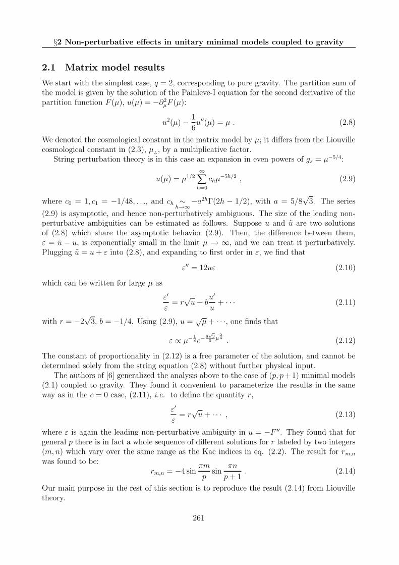
§2 Non-perturbative effects in unitary minimal models coupled to gravity
2.1 Matrix model results
We start with the simplest case, q = 2, corresponding to pure gravity. The partition sum ofthe model is given by the solution of the Painleve-I equation for the second derivative of thepartition function F (µ), u(µ) = −∂2
µF (µ):
u2(µ) − 1
6u′′(µ) = µ . (2.8)
We denoted the cosmological constant in the matrix model by µ; it differs from the Liouvillecosmological constant in (2.3), µ
L, by a multiplicative factor.
String perturbation theory is in this case an expansion in even powers of gs = µ−5/4:
u(µ) = µ1/2∞∑
h=0
chµ−5h/2 , (2.9)
where c0 = 1, c1 = −1/48, . . ., and ch ∼h→∞
−a2hΓ(2h − 1/2), with a = 5/8√
3. The series
(2.9) is asymptotic, and hence non-perturbatively ambiguous. The size of the leading non-perturbative ambiguities can be estimated as follows. Suppose u and u are two solutionsof (2.8) which share the asymptotic behavior (2.9). Then, the difference between them,ε = u − u, is exponentially small in the limit µ → ∞, and we can treat it perturbatively.Plugging u = u+ ε into (2.8), and expanding to first order in ε, we find that
ε′′ = 12uε (2.10)
which can be written for large µ as
ε′
ε= r
√u+ b
u′
u+ · · · (2.11)
with r = −2√
3, b = −1/4. Using (2.9), u =√µ+ · · ·, one finds that
ε ∝ µ− 18 e−
8√
35µ
54 . (2.12)
The constant of proportionality in (2.12) is a free parameter of the solution, and cannot bedetermined solely from the string equation (2.8) without further physical input.
The authors of [6] generalized the analysis above to the case of (p, p+1) minimal models(2.1) coupled to gravity. They found it convenient to parameterize the results in the sameway as in the c = 0 case, (2.11), i.e. to define the quantity r,
ε′
ε= r
√u+ · · · , (2.13)
where ε is again the leading non-perturbative ambiguity in u = −F ′′. They found that forgeneral p there is in fact a whole sequence of different solutions for r labeled by two integers(m,n) which vary over the same range as the Kac indices in eq. (2.2). The result for rm,nwas found to be:
rm,n = −4 sinπm
psin
πn
p+ 1. (2.14)
Our main purpose in the rest of this section is to reproduce the result (2.14) from Liouvilletheory.
261

Article VI: Non-perturbative effects in matrix models and D-branes
2.2 Liouville analysis
As discussed in the introduction, general considerations suggest that the leading non-perturbative effects in string theory should be due to contributions of world sheets withholes, with boundary conditions corresponding to localized D-branes. The first questionthat we need to address is which D-branes should be considered for this analysis.
The minimal model part of the background can be thought of as a finite collection ofpoints. All D-branes corresponding to it are localized and therefore should contribute tothe non-perturbative effects. Minimal model D-branes are well understood [17]. They are inone to one correspondence with primaries of the Virasoro algebra (2.2). For our purposes,the main property that will be important is the disk partition sum (or boundary entropy)corresponding to the (m,n) brane, which is given by
Zm,n =
(
8
p(p+ 1)
)1/4 sin πmp
sin πnp+1
(
sin πp
sin πp+1
)1/2. (2.15)
What about the Liouville part of the background? The authors of [11] introduced an infinitesequence of localized D-branes, labeled by two integers (m′, n′). Which of these branes shouldwe take in evaluating instanton effects?
The analysis of [11] shows that open strings stretched between the (m′, n′) and (m′′, n′′)Liouville branes belong to one of a finite number of degenerate representations of the Vi-rasoro algebra with central charge (2.4). The precise set of degenerate representations thatarises depends on m′, n′, m′′, n′′. Degenerate representations at c > 25 occur at negative val-ues of world sheet scaling dimension, except for the simplest degenerate operator, 1, whosedimension is zero. One finds [11] that in all sectors of open strings, except those correspond-ing to m′ = n′ = m′′ = n′′ = 1 there are negative dimension operators. It is thus natural toconjecture that the only stable D-instantons correspond to the case (m′, n′) = (1, 1), and wewill assume this in the analysis below.
To recapitulate, the D-instantons that give rise to the non-perturbative effects in c < 1minimal models coupled to gravity have the form: (1, 1) brane in Liouville × (m,n) branein the minimal model. We next show that these D-branes give rise to the correct leadingnon-perturbative effects (2.14).
In order to compare to the matrix model results we should in principle use eq. (1.2), andevaluate the disk partition sum of the Liouville × minimal model D-brane. It turns out,however, much more convenient to compare directly the quantity r (2.13) which appearsnaturally in the matrix model analysis. The basic point is that this quantity is a naturalobject to consider in the continuum approach as well.
Indeed, from the continuum point of view, r is the ratio
r =∂∂µ
log ε√u
=
∂∂µ
LZdisc
√
−∂2µ
LF, (2.16)
where in the numerator we used the fact that log ε is the disk partition sum corresponding tothe D-instanton (see (1.2)). Thus we see that r is the ratio between the one point functionof the cosmological constant operator Vb on the disk, and the square root of its two point
262
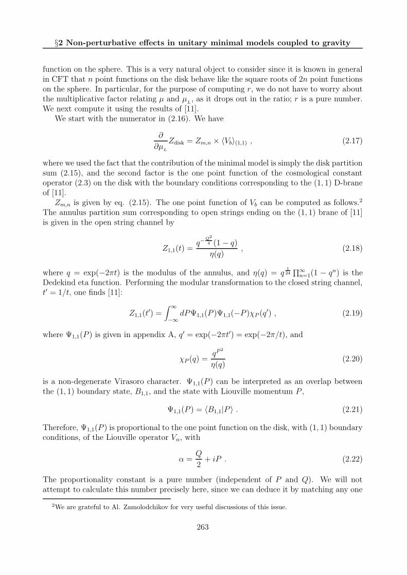
§2 Non-perturbative effects in unitary minimal models coupled to gravity
function on the sphere. This is a very natural object to consider since it is known in generalin CFT that n point functions on the disk behave like the square roots of 2n point functionson the sphere. In particular, for the purpose of computing r, we do not have to worry aboutthe multiplicative factor relating µ and µ
L, as it drops out in the ratio; r is a pure number.
We next compute it using the results of [11].We start with the numerator in (2.16). We have
∂
∂µL
Zdisk = Zm,n × 〈Vb〉(1,1) , (2.17)
where we used the fact that the contribution of the minimal model is simply the disk partitionsum (2.15), and the second factor is the one point function of the cosmological constantoperator (2.3) on the disk with the boundary conditions corresponding to the (1, 1) D-braneof [11].
Zm,n is given by eq. (2.15). The one point function of Vb can be computed as follows.2
The annulus partition sum corresponding to open strings ending on the (1, 1) brane of [11]is given in the open string channel by
Z1,1(t) =q−
Q2
4 (1 − q)
η(q), (2.18)
where q = exp(−2πt) is the modulus of the annulus, and η(q) = q124∏∞n=1(1 − qn) is the
Dedekind eta function. Performing the modular transformation to the closed string channel,t′ = 1/t, one finds [11]:
Z1,1(t′) =
∫ ∞
−∞dPΨ1,1(P )Ψ1,1(−P )χP (q′) , (2.19)
where Ψ1,1(P ) is given in appendix A, q′ = exp(−2πt′) = exp(−2π/t), and
χP (q) =qP
2
η(q)(2.20)
is a non-degenerate Virasoro character. Ψ1,1(P ) can be interpreted as an overlap betweenthe (1, 1) boundary state, B1,1, and the state with Liouville momentum P ,
Ψ1,1(P ) = 〈B1,1|P 〉 . (2.21)
Therefore, Ψ1,1(P ) is proportional to the one point function on the disk, with (1, 1) boundaryconditions, of the Liouville operator Vα, with
α =Q
2+ iP . (2.22)
The proportionality constant is a pure number (independent of P and Q). We will notattempt to calculate this number precisely here, since we can deduce it by matching any one
2We are grateful to Al. Zamolodchikov for very useful discussions of this issue.
263

Article VI: Non-perturbative effects in matrix models and D-branes
of the matrix model predictions, and then use it in all other calculations, but we will nextmention a few contributions to it, for illustrative purposes.
First, in (2.19) the P integral runs over the whole real line, but |P 〉 and | − P 〉 are thesame state, due to reflection from the Liouville wall, so we should replace
∫∞−∞ dP = 2
∫∞0 dP .
Hence, the physical wavefunctions which should appear in (2.21) are√
2Ψ1,1. Furthermore,the state |P 〉 in (2.21) is normalized as 〈P |P ′〉 = δ(P − P ′), for consistency with (2.19). Onthe other hand, the state created by acting with the Liouville exponential Vα (2.7), with αgiven by (2.22), is normalized to πδ(P − P ′). Finally, when computing 〈Vα(0)〉disk, the partof the SL(2,R) symmetry of the disk related to rotations around the origin is unfixed. Thisgives an extra factor of 1/2π in the one point function. Altogether, one finds
〈Vα(0)〉(1,1) = C ·√
2 · √π · 1
2π· Ψ1,1 (2.23)
where α is given by (2.22) and C is an undetermined constant which we will fix by comparingto matrix model results (we will find that C = 2).
We can now plug in (2.23) into (2.17) and, using the form of Ψ1,1 given in (A3), find
〈Vb(0)〉(1,1) = −C 21/4√π[πµ
Lγ(b2)]
12(1/b2−1)
bΓ(1 − b2)Γ(1/b2). (2.24)
We next move on to the denominator of (2.16). This is given by the two point function〈VbVb〉sphere. This quantity was calculated in [18, 19]. It is convenient to first compute thethree point function 〈VbVbVb〉sphere and then integrate once, to avoid certain subtle questionsregarding the fixing of the SL(2, C) Conformal Killing Group of the sphere. One has (seeappendix A):
〈VbVbVb〉sphere = b−1 [πµL]1/b
2−2 [γ(b2)]1/b2
γ(2 − 1/b2) . (2.25)
Integrating once w.r.t. −µL
we find
〈VbVb〉sphere =1/b2 − 1
πb
[
πµLγ(b2)
]1/b2−1γ(b2)γ(1 − 1/b2) . (2.26)
We are now ready to compute r, (2.16). Plugging in (2.15), (2.24) and (2.26) into (2.16), wefind
rm,n = −2C sinπm
psin
πn
p+ 1, (2.27)
which agrees with the matrix model result (2.14) if we set C = 2. Since C is independentof m, n and p, we can fix it by matching to any one case, and then use it in all others. Weconclude that the Liouville analysis gives the same results as the matrix model one.
3 Non-perturbative effects in compactified c = 1 string
theory
In this section we discuss the leading non-perturbative effects in (Euclidean) two dimensionalstring theory. The world sheet description contains a field x, compactified on a circle of radius
264

§3 Non-perturbative effects in compactified c = 1 string theory
R, x ' x+2πR, coupled to gravity. The conformal gauge Lagrangian describing this systemis
L =1
4π
[
(∂x)2 + (∂φ)2 + 2Rφ+ µLφe2φ + λe(2−R)φ cos[R(xL − xR)]
]
. (3.1)
where we chose α′ = 1, and perturbed the c = 1 model by a Sine-Gordon type interaction,λ cos[R(xL − xR)], which gives rise to the last term in (3.1) after coupling to gravity. Theperturbation is relevant for R < 2, and we will restrict to that case in the discussion below.
We will next describe the matrix model predictions for the leading non-perturbativeeffects corresponding to (3.1), and then verify some of them in Liouville theory.
3.1 Matrix model analysis
The model (3.1) was solved using matrix model techniques in [15], extending some earlierresults [20, 21, 22, 23, 24]. In particular, it was shown in [15] that the Legendre transformF of the string partition sum F satisfies the Toda differential equation:
1
4λ−1∂λλ∂λF(µ, λ) + exp
[
−4 sin2
(
1
2
∂
∂µ
)
F(µ, λ)
]
= 1 . (3.2)
The initial condition for this equation is supplied by the unperturbed c = 1 string theory ona circle
F(µ, 0) = R4
Re∫∞Λ−1
dss
e−iµs
sinh s2
sinh s2R
= −R2µ2 log µ
Λ− 1
24(R + 1
R) log µ
Λ+R
∑∞h=2 µ
2−2hch(R) +O(e−2πµ) +O(e−2πRµ) , (3.3)
where the genus h term ch(R) is a known polynomial in 1/R. The function F(λ, µ) has agenus expansion which follows from (3.2). The string partition sum F is obtained from Fby flipping the sign of the genus zero term [25].
We will need below some features of the solution of equations (3.2), (3.3), which wereview next. In order to study the solution of (3.2), (3.3), it is convenient to introduce theparameters
y = µξ, ξ = (λ√R− 1)−
22−R . (3.4)
This parameterization is useful when λ is large, so that the last term in (3.1) sets the scale,and one can study the cosmological term perturbatively in µ. As explained in [15], this canonly be done for R > 1. This is the physical origin of the branch cut in the definition of ξ in(3.4). In the regime where λ sets the scale, the genus expansion of the string partition sumis an expansion in even powers of ξ:
F(µ, λ) = λ2 + ξ−2[
R
2y2 log ξ + f0(y)
]
+
[
R +R−1
24log ξ + f1(y)
]
+∞∑
h=2
ξ2h−2fh(y) . (3.5)
The partition sum on the sphere, F0(µ, λ), is given by the second term on the r.h.s. of (3.5).One can show [15] that at this order, the full Toda equation (3.2) reduces to an algebraicequation for X = ∂2
yf0
y = e−1RX − e−
R−1R
X . (3.6)
265

Article VI: Non-perturbative effects in matrix models and D-branes
This leads to the following perturbative expansion of F0(µ, λ) in powers of λ:
F0(µ, λ) =R
2µ2 log
Λ
µ+Rµ2
∞∑
n=1
1
n!
(
(1 − R)µR−2λ2)n Γ(n(2 − R) − 2)
Γ(n(1 − R) + 1), (3.7)
which agrees with the original (conjectured) result for this quantity in [20]. The genus h ≥ 1terms in the expansion (3.5) can be computed in principle by substituting (3.5) into (3.2),but only f0 and f1 are known in closed form. Nevertheless, we will see below that the largeh behavior of fh can be obtained directly from the differential equation (3.2), by computingthe leading non-perturbative corrections to (3.5). We next turn to these corrections.
At λ = 0, there are two types of non-perturbative corrections to the 1/µ expansion (3.3),associated with the poles of the integrand in that equation. These occur at s = 2πik ands = 2πRik, k ∈ Z, and give rise to the non-perturbative effects indicated on the second lineof (3.3), exp(−2πµk) and exp(−2πRµk), respectively.
At finite λ, the situation is more interesting. The series of non-perturbative corrections
∆F =∞∑
n=1
Cne−2πnµ (3.8)
gives rise to an exact solution of the full equation (3.2) [15]. Thus, the correspondinginstantons are insensitive to the presence of the sine-Gordon perturbation! We will return tothis interesting fact, and explain its interpretation in Liouville theory, in the next subsection.
The second type of corrections, which starts at λ = 0 like ∆F = e−2πRµ, does not solvethe full equation (3.2), and gets λ dependent corrections. To study these corrections one canproceed in a similar way to that described in section 2.1.
Let F and F = F+ε be two solutions of the Toda equation (3.2). The linearized equationfor ε reads
1
4λ−1∂λλ∂λε(µ, λ) − 4e−∂
2µF0(µ,λ) sin2
(
1
2
∂
∂µ
)
ε(µ, λ) = 0 , (3.9)
where in the exponential in the second term we approximated
4 sin2
(
1
2
∂
∂µ
)
F(µ, λ) ' ∂2µF0 = R log ξ +X(y) . (3.10)
This is similar to the fact that in the discussion of section 2, one can replace u in eq. (2.10)by its limit as µ→ ∞. After the change of variables from (λ, µ) to (y, µ), equation (3.9) canbe written as
αy2
µ2(y∂y)
2ε(µ, y)− 4e−X(y) sin2
(
1
2
(
∂
∂µ+y
µ
∂
∂y
))
ε(µ, y) = 0 , (3.11)
where α ≡ R−1(2−R)2
.Since we know that ε is non-perturbatively small in the µ→ ∞ limit, we use the following
ansatz for it:ε(µ, y) = P (µ, y)e−µf(y) . (3.12)
Here P is a power-like prefactor in gs, and f(y) is the function we are interested in (theanalogue of r in the minimal models of section 2). Substituting (3.12) into (3.11) and keeping
266

§3 Non-perturbative effects in compactified c = 1 string theory
only the leading terms in the µ → ∞ limit, one finds the following first order differentialequation: √
α e12X(y)(1 − y∂y)g(y) = ± sin [∂yg(y)] , (3.13)
where we introduced
g(y) =1
2yf(y) . (3.14)
The ± in (3.13) is due to the fact that one in fact finds the square of this equation.Equation (3.13) is a first order differential equation in y, and to solve it we need to specify
boundary conditions. As discussed earlier for the perturbative series, it is natural to specifythese boundary conditions at λ → 0, or y → ∞ (see (3.4)). We saw in the discussion of(3.3) that there are two solutions, f(y → ∞) → 2π or 2πR. This implies via (3.14) thatg(y → ∞) ' πy or πRy. We already saw that g(y) = πy gives an exact solution of (3.2), andthis is true for (3.13) as well (as it should be). Thus, to study non-trivial non-perturbativeeffects, we must take the other boundary condition,
g(y → ∞) ' πRy . (3.15)
Interestingly, eq. (3.13) is exactly solvable. We outline the solution in Appendix B. Forthe initial condition (3.15), the solution can be written as
g(y) = yφ(y)± 1√αe−
12X(y) sin φ(y) , (3.16)
where φ(y) = ∂yg satisfies the equation
e2−R2R
X(y) = ±√R− 1
sin(
1Rφ)
sin(
R−1Rφ) . (3.17)
The solution with the minus sign in (3.17) can be shown to be unphysical (see below). Wewill thus use the solution with a plus sign.
Equations (3.16), (3.17) are the main result of this subsection. We next discuss somefeatures of the corresponding non-perturbative effects.
Consider first the situation for small λ, or large y. The first three terms in the expansionof φ(y) are
φ(y) ≈ πR± R sin(πR)√R− 1
y−2−R
2 +R
2sin(2πR) y−(2−R) . (3.18)
This gives the following result for f(y) (3.12):
f(y) = 2πR± 4 sin(πR)√R− 1
y−2−R
2 +R sin(2πR)
R− 1y−(2−R) +O(y−3(2−R)/2)
= 2πR± 4 sin(πR)µ− 2−R2 λ +R sin(2πR)µ−(2−R) λ2 +O(λ3) . (3.19)
We see that for large y, the expansion parameter is y−(2−R)
2 ∼ λ, as one would expect.Another interesting limit is µ→ 0 at fixed λ, i.e. y → 0, which leads to the Sine-Liouville
model, (3.1) with µL
= 0. For R = 3/2, this model is equivalent to the Euclidean black hole
267

Article VI: Non-perturbative effects in matrix models and D-branes
background [26, 15]. As we see in (3.6), in this limit X → 0. The first two terms in theexpansion of φ around this point are
φ(y) = φ0 +R
2
(
(R− 1) cot(
R− 1
Rφ0
)
− cot(
1
Rφ0
))−1
y +O(y2) , (3.20)
where φ0 is defined by the equation
sin(
1Rφ0
)
sin(
R−1Rφ0
) = ± 1√R− 1
. (3.21)
The function f(y) is given in this limit by the expansion
f(y) = ± 2(2 − R)
y√R− 1
sinφ0 + 2φ0 +O(y) . (3.22)
Note that the behavior of f as y → 0, f ∼ 1/y, leads to a smooth limit as µ→ 0 at fixed λ.The non-perturbative effect (3.12) goes like exp(−µf(y)), so that as y → 0 the argument ofthe exponential goes like µ/y = 1/ξ, and all dependence on µ disappears.
For R = 3/2, which corresponds to the Euclidean black hole, the equations simplify. Onecan explicitly find φ0 because (3.21) gives
cosφ0
3= ± 1√
2⇒ φ0 =
3π
4or φ0 =
9π
4. (3.23)
As a result, one finds at this value of the radius a simple result
µf(y) = ±µy
+(6 ∓ 3)π
2µ+ · · · = ±1
2λ4 +
(6 ∓ 3)π
2µ+ · · · . (3.24)
In fact, for the particular case R = 3/2 one can find f(y) exactly. The result is given inAppendix B. Note that the solution with the minus sign leads to a growing exponential,e
12λ4
. Therefore, it is not physical, as mentioned above.Another nice consistency check on our solution is the RG flow from c = 1 to c = 0
CFT coupled to gravity, implicit in (3.1). Before coupling to gravity, the Sine-Gordon modelassociated to (3.1) describes the following RG flow. In the UV, the Sine-Gordon couplingeffectively goes to zero, and one approaches the standard CFT of a compact scalar field. Inthe IR, the potential given by the Sine-Gordon interaction gives a world sheet mass to x,and the model approaches a trivial c = 0 fixed point. As shown in [20, 22], this RG flowmanifests itself after coupling to gravity in the dependence of the physics on µ. Large µcorresponds to the UV limit; in it, all correlators approach those of the c = 1 theory coupledto gravity. Decreasing µ corresponds in this language to the flow to the IR, with the c = 0behavior recovered as µ approaches a critical value µc, which is given by:
µc = −(2 − R)(R− 1)R
2−Rλ2
2−R . (3.25)
The non-perturbative contributions to the partition sum computed in this section must followa similar pattern. In particular, f(y) must exhibit a singularity as y → yc, with
yc = −(2 − R)(R− 1)R−12−R (3.26)
268

§3 Non-perturbative effects in compactified c = 1 string theory
and furthermore, the behavior of f near this singularity should reproduce the non-perturbative effects of the c = 0 model coupled to gravity discussed in section 2.
The singularity at y = yc corresponds to a critical point of (3.6), near which the relationbetween y and X degenerates:
yc − y
yc' R − 1
2R2(X −Xc)
2 +O(
(X −Xc)3)
. (3.27)
Solving for the critical point, one finds that
e−2−R2R
Xc =√R − 1 . (3.28)
The corresponding yc is indeed given by (3.26). We can now solve for f(y), near y = yc.Substituting (3.28) in (3.17) we find
sin(
1Rφ)
sin(
R−1Rφ) =
1
R− 1. (3.29)
Thus, the c = 0 critical point corresponds to φ → 0.3 The first two terms in the expansionof φ around the singularity are
φ(y) =√
3(Xc −X)1/2 −√
3(R2 − 2R+ 2)
20R2(Xc −X)3/2 +O
(
(Xc −X)5/2)
. (3.30)
Substituting this in (3.16) one finds
g(y) = −yc2√
3(R − 1)
5R2(Xc −X)5/2 +O
(
(Xc −X)5/2)
(3.31)
or, using (3.14):
f(y) ≈ −8√
3
5
(
2R2
R− 1
)1/4 (µc − µ
µc
)5/4
. (3.32)
The power of µ − µc is precisely right to describe a leading non-perturbative effect in puregravity. It is interesting to compare the coefficient in (3.32) to what is expected in puregravity. It is most convenient to do this by again computing r (2.11). u is computed byevaluating the leading singular term as µ→ µc in ∂2
µF0 = R logχ +X(y). One finds
r = −2√
3
(
2R2
R− 1
)1/4 (µc − µ
µc
)1/4
(Xc −X)−1/2 = −2√
3 (3.33)
in agreement with the result (2.14) for pure gravity. This provides another non-trivialconsistency check of our solution.
3Note that if we chose the minus sign in (3.17), we would find a more complicated solution for φ. Onecan show that it would lead to the wrong critical behavior. This is an additional check of the fact that thephysical solution corresponds to the plus sign in (3.17).
269

Article VI: Non-perturbative effects in matrix models and D-branes
3.2 Liouville analysis
In this subsection we will discuss the Liouville interpretation of the matrix model resultspresented in the previous subsection. Consider first the unperturbed c = 1 theory corre-sponding to λ = 0 in (3.1). As we saw, in the matrix model analysis one finds two differenttypes of leading non-perturbative effects (see (3.3)), exp(−2πµ), and exp(−2πRµ). It isnot difficult to guess the origin of these non-perturbative effects from the Liouville point ofview. The exp(−2πµ) contribution is due to a D-brane that corresponds to a (1, 1) Liouvillebrane × a Dirichlet brane in the c = 1 CFT, i.e. a brane located at a point on the circleparameterized by x. Similarly, the exp(−2πRµ) term comes from a brane wrapped aroundthe x circle.
This identification can be verified in the same way as we did for minimal models in section2. To avoid normalization issues, one can again calculate the quantity r (2.16). The matrixmodel prediction for the Neumann brane4 is
r = − 2π√R
√
log Λµ
, (3.34)
where we used the sphere partition function F0(µ, 0) of the unperturbed compactified c = 1string given by the first term in (3.7).
The CFT calculation is similar to that performed in the c < 1 case. The partitionfunction of c = 1 CFT on a disk with Neumann boundary conditions is well known; thecalculation is reviewed in Appendix C. One finds
ZNeumann = 2−1/4√R . (3.35)
The disk amplitude corresponding to the (1, 1) Liouville brane, and the two-point functionon the sphere are computed using equations (2.24) and (2.26), in the limit b→ 1. The limitis actually singular, but computing everything for generic b and taking the limit at the endof the calculation leads to sensible, finite results. The leading behavior of (2.24) as b→ 1 is
〈Vb(0)〉(1,1) ≈ − 25/4√π
Γ(1 − b2), (3.36)
with the constant C in (2.24) chosen to be equal to 2, as in the minimal model analysis ofequations (2.23) – (2.27). The two point function (2.26) approaches
∂2µ
LF0 ' − logµ
L
πΓ2(1 − b2). (3.37)
Substituting (3.35), (3.36) and (3.37) into (2.16) gives the result (3.34). This provides anon-trivial check of the statement in section 2, that the constant C in eq. (2.23) is a purenumber, independent of all the parameters of the model.
The agreement of (3.34) with the Liouville analysis supports the identification of theNeumann D-branes as the source of the non-perturbative effects exp(−2πRµ). A similar
4Similar formulae can be written for the Dirichlet brane.
270

§3 Non-perturbative effects in compactified c = 1 string theory
analysis leads to the same conclusion regarding the relation between the Dirichlet c = 1branes and the non-perturbative effects exp(−2πµ) (the two kinds of branes are related byT-duality).
Having understood the structure of the unperturbed theory, we next turn to the theorywith generic λ. In the matrix model we found that the non-perturbative effects associatedwith the Dirichlet brane localized on the x circle are in fact independent of λ (see (3.8) andthe subsequent discussion). How can we understand this statement from the Liouville pointof view?
The statement that (3.8) is an exact solution of the Toda equation (3.2) corresponds inthe continuum formulation to the claim that the disk partition sum of the model (3.1), with(1, 1) boundary conditions for Liouville, and Dirichlet boundary conditions for the matterfield x is independent of λ. In other words, all n-point functions of the operator given bythe last term in (3.1) on the disk vanish
⟨(∫
d2ze(2−R)φ cos[R(xL − xR)])n⟩
(1,1)×Dirichlet= 0 . (3.38)
Is it reasonable to expect (3.38) to be valid from the world sheet point of view? For oddn (3.38) is trivially zero because of winding number conservation. Indeed, the Dirichletboundary state for x breaks translation invariance, but preserves winding number. Theperturbation in (3.1) carries winding number, and for odd n all terms in (3.38) have non-zero winding number. Thus, the correlator vanishes.
For even n one has to work harder, but it is still reasonable to expect the amplitudeto vanish in this case. Indeed, consider the T-dual statement to (3.38), that the n pointfunctions of the momentum mode cos(x/R), on the disk with (1, 1) × Neumann boundaryconditions, vanish. This is reasonable since the operator whose correlation functions arebeing computed localizes x at the minima of the cosine, while the D-brane on which thestring ends is smeared over the whole circle. It might be possible to make this argumentprecise by using the fact that in this case the D-instanton preserves a different symmetryfrom that preserved by the perturbed theory, and thus it should not contribute to the non-perturbative effects.
To summarize, the matrix model analysis predicts that (3.38) is valid. We will notattempt to prove this assertion here from the Liouville point of view (it would be niceto verify it even for the simplest case, n = 2), and instead move on to discuss the non-perturbative effects due to the localized branes on the x circle.
The non-trivial solution of eq. (3.13) given by (3.16), (3.17) should correspond fromthe Liouville point of view to the disk partition sum of the (1, 1) Liouville brane which iswrapped around the x circle. The prediction is that
⟨(∫
d2ze(2−R)φ cos[R(xL − xR)])n⟩
(1,1)×Neumann(3.39)
are the coefficients in the expansion of f(y) (3.12) in a power series in λ, the first termsof which are given by (3.19). It would be very nice to verify this prediction directly usingLiouville theory, but in general this seems hard given the present state of the art. A simplecheck that can be performed using results in [11] is to compare the order λ term in (3.19)with the n = 1 correlator (3.39). We next compare the two.
271

Article VI: Non-perturbative effects in matrix models and D-branes
Like in the other cases studied earlier, it is convenient to define a dimensionless quantity,ρ, given by the ratio of the one point function on the disk (3.39) and the square root of theappropriate two point function on the sphere,
ρ =∂∂λ
log ε√
−∂2λF0
∣
∣
∣
∣
∣
∣
λ=0
. (3.40)
The matrix model result (3.19), (3.7), for this quantity is
ρ = − µ ∂∂λf
√
−∂2λF0
∣
∣
∣
∣
∣
∣
λ=0
= −2√
2 sin(πR) . (3.41)
In the Liouville description, ρ is given by
ρ =BT 〈Vb−R
2〉(1,1)
√
−〈T 2〉. (3.42)
Here, T = cosR(xL − xR)Vb−R2. BT is the one point function of cosR(xL − xR) on the disk.
It has the same value as (3.35) (see appendix C)
BT = 2−1/4√R . (3.43)
The one-point function of the operator of Vb−R2
is related to the wavefunction (A.3) with
momentum iP = b− R/2 −Q/2 and is given by
〈Vb−R2(0)〉(1,1) = − 25/4
√π[πµ
Lγ(b2)]
12(1/b2−1+R/b)
bΓ(1 − b2 +Rb)Γ(1/b2 +R/b). (3.44)
The two-point function of T on the sphere is computed as above from the three pointfunction (A.10). One finds
⟨
T 2⟩
=
(
1b2
+ Rb− 1
)
2πb
[
πµLγ(b2)
] 1b2
+Rb−1γ(
b2 − Rb)
γ(
1 − 1
b2− R
b
)
. (3.45)
Substituting these results into (3.42) leads, in the limit b = 1, to (3.41). We see thatthe Liouville results are again in complete agreement with the corresponding matrix modelcalculation.
4 Discussion
In this paper we studied non-perturbative effects in c ≤ 1 non-critical string theory, usingboth matrix model and continuum (Liouville) methods. We showed that the matrix modelresults correspond in the continuum approach to D-instanton effects due to localized branesin Liouville theory, the (1, 1) branes constructed in [11]. Our work is motivated by the recentproposal of [12], but the details are different.
272

§4 Discussion
For c < 1 unitary minimal models, we showed that the contribution of these branesreproduces the matrix model results of [6]. For c = 1 we used the results of [15] to derivethe leading non-perturbative effects in the matrix model description of the Sine-Gordonmodel coupled to gravity, as a function of the compactification radius and the Sine-Gordoncoupling, and reproduced some of these predictions using the Liouville branes of [11].
The matrix model analysis led in addition to a number of predictions regarding theproperties of D-instantons in c = 1 string theory. In particular, we showed that an infinitenumber of correlation functions given in eq. (3.38) must vanish, and the correlation functions(3.39) are given by the expansion of f(y) (3.14) in a power series in λ, the first few terms ofwhich appear in (3.19).
Another interesting set of matrix model predictions concerns the limit µ → 0, in whichone finds the Sine-Liouville model, (3.1) with µL = 0. The expansion of f(y) around y = 0,(3.22), provides information about the disk partition sum and correlation functions of closedstring operators in the presence of D-branes in this model. For the particular case R =3/2, these predictions apply also to the SL(2)/U(1) (cigar) background corresponding to aEuclidean two dimensional black hole. In the cigar, the D-branes in question are wrappedaround the angular direction of the cigar, and are localized near the tip. Our results giverise to predictions for correlation functions on the disk with these boundary conditions.
Our analysis also resolves a previously open problem, of describing world sheet gravityon the disk with the boundary conditions described in [11] using the matrix model approach.It opens the possibility of studying gravity on AdS2 using matrix model techniques.
An interesting open problem is how to go beyond the calculation of the leading non-perturbative contributions to the amplitudes (1.1), and study the perturbative expansionaround the D-instantons discussed in this paper. In the matrix model approach one findsthat the leading non-perturbative terms behave like
A1−inst. ∼ C gfAs e−
fDgs , (4.1)
where fD was discussed in this paper, and fA is known as well.5 The constant C is ambiguousin the matrix model.
In the continuum Liouville description, fD has been computed in this paper, and it wouldbe interesting to compute fA and understand whether C is ambiguous or can be determined.In order to study these issues, one has to understand the perturbative expansion about theD-instantons discussed in this paper. In particular, it is natural to expect that fA will arisefrom the annulus with boundary conditions corresponding to the (1, 1) brane (this gives thecorrect scaling with gs).
The discussion of this paper has some interesting higher dimensional generalizations. Forexample, if one replaces Liouville by N = 2 Liouville, and the minimal models by N = 2minimal models, one finds the background
SL(2)kU(1)
× SU(2)kU(1)
(4.2)
5For the partition sum one finds a simple universal behaviour. For the minimal models, in all cases
that we are aware of, Fnon−pert ∼ g1/2s e−
fDgs (see [27]). For the c = 1 model, equation (3.8) suggests that
Fnon−pert ∼ g0se
−fDgs .
273

Article VI: Non-perturbative effects in matrix models and D-branes
describing NS5-branes spread out on a circle [28, 29]. The D-instantons analogous to thosestudied in this paper correspond to Euclidean D0-branes stretched between pairs of five-branes. From the point of view of the geometry (4.2), they are described by D-branes livingnear the tip of the cigar, which are N = 2 superconformal generalizations of the (1, 1) braneof [11]. In particular, the spectrum of open strings ending on them corresponds to the N = 2superconformal block of the identity.
Like in our case, the D-instantons are obtained by tensoring the above N = 2 Liouvillebranes with the different D-branes in the N = 2 minimal model. Understanding the non-perturbative effects due to these instantons is an interesting open problem. Studying thebranes discussed in this paper in more detail is a very useful warmup exercise for the fivebraneproblem. It might suggest hints for finding an analog of the matrix model for fivebranes.
Acknowledgements: We thank V. Fateev, A. Giveon, I. Kostov, E. Martinec, G. Moore,and especially Al. Zamolodchikov for useful discussions. The work of V.K. is supported inpart by NATO grant PST.CLG.978817. The work of D.K. is supported in part by DOE grant#DE-FG02-90ER40560. D.K. thanks LPT at Ecole Normale Superieure (Paris), LPTHE atUniversite Paris VI, and LPM at Universite Montpellier II for hospitality during the courseof this work. The work of S.A. and V.K. was partially supported by European Union underthe RTN contracts HPRN-CT-2000-00122 and -00131. The work of S.A. was also supportedin part by European network EUCLID HPRN-CT-2002-00325.
Appendix A. Correlation functions in Liouville theory.
In this appendix we summarize some results on Liouville field theory, from [11, 18, 19], whichare used in the text. The one-point function of the operator (2.7) in Liouville theory on thedisk with boundary conditions corresponding to the (1, 1) brane is given by
U(α) =[πµ
Lγ(b2)]−α/bQΓ(bQ)Γ(Q/b)
(Q− 2α)Γ(b(Q− 2α))Γ((Q− 2α)/b), (A.1)
where
γ(x) =Γ(x)
Γ(1 − x). (A.2)
U(α) is the normalized one-point function, i.e. the one point function divided by the diskpartition function. As discussed in the text, the unnormalized one point function of Vα isrelated to the wavefunction with momentum iP = α−Q/2 defined by (2.19), which is givenby
Ψ1,1(P ) =23/42πiP [πµ
Lγ(b2)]−iP/b
Γ(1 − 2ibP )Γ(1 − 2iP/b). (A.3)
The three-point function on the sphere is (suppressing the standard dependence on theworld sheet positions of the vertex operators)
〈Vα1Vα2Vα3〉sphere =[
πµLγ(b2)b2−2b2
](Q−∑
αi)/b×Υ0Υ(2α1)Υ(2α2)Υ(2α3)
Υ(α1+α2+α3−Q)Υ(α1+α2−α3)Υ(α2+α3−α1)Υ(α3+α1−α2), (A.4)
274
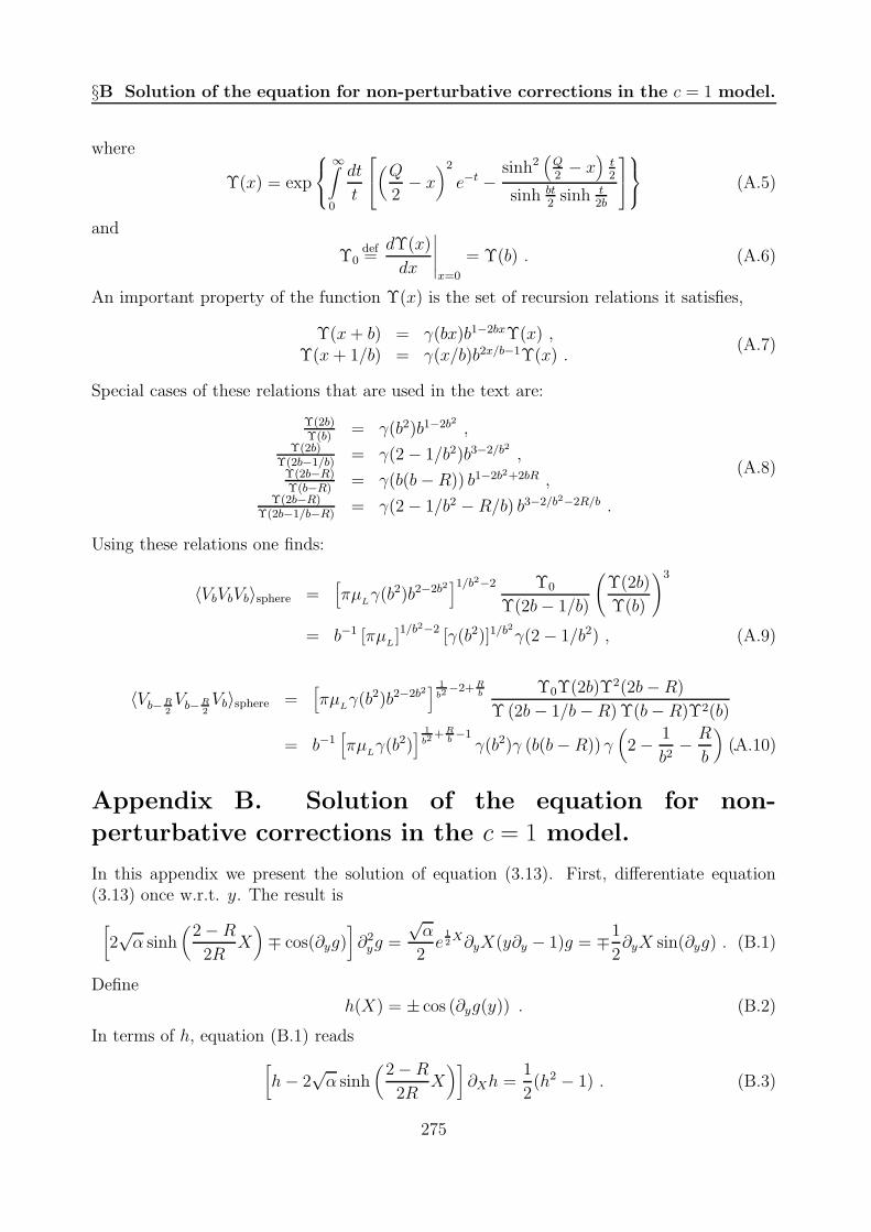
§B Solution of the equation for non-perturbative corrections in the c = 1 model.
where
Υ(x) = exp
∞∫
0
dt
t
(
Q
2− x
)2
e−t −sinh2
(
Q2− x
)
t2
sinh bt2
sinh t2b
(A.5)
and
Υ0def=dΥ(x)
dx
∣
∣
∣
∣
∣
x=0
= Υ(b) . (A.6)
An important property of the function Υ(x) is the set of recursion relations it satisfies,
Υ(x+ b) = γ(bx)b1−2bxΥ(x) ,Υ(x+ 1/b) = γ(x/b)b2x/b−1Υ(x) .
(A.7)
Special cases of these relations that are used in the text are:
Υ(2b)Υ(b)
= γ(b2)b1−2b2 ,Υ(2b)
Υ(2b−1/b)= γ(2 − 1/b2)b3−2/b2 ,
Υ(2b−R)Υ(b−R)
= γ(b(b−R)) b1−2b2+2bR ,Υ(2b−R)
Υ(2b−1/b−R)= γ(2 − 1/b2 − R/b) b3−2/b2−2R/b .
(A.8)
Using these relations one finds:
〈VbVbVb〉sphere =[
πµLγ(b2)b2−2b2
]1/b2−2 Υ0
Υ(2b− 1/b)
(
Υ(2b)
Υ(b)
)3
= b−1 [πµL]1/b
2−2 [γ(b2)]1/b2
γ(2 − 1/b2) , (A.9)
〈Vb−R2Vb−R
2Vb〉sphere =
[
πµLγ(b2)b2−2b2
] 1b2
−2+ Rb Υ0Υ(2b)Υ2(2b− R)
Υ (2b− 1/b−R) Υ(b− R)Υ2(b)
= b−1[
πµLγ(b2)
] 1b2
+Rb−1γ(b2)γ (b(b− R)) γ
(
2 − 1
b2− R
b
)
.(A.10)
Appendix B. Solution of the equation for non-
perturbative corrections in the c = 1 model.
In this appendix we present the solution of equation (3.13). First, differentiate equation(3.13) once w.r.t. y. The result is
[
2√α sinh
(
2 − R
2RX)
∓ cos(∂yg)]
∂2yg =
√α
2e
12X∂yX(y∂y − 1)g = ∓1
2∂yX sin(∂yg) . (B.1)
Defineh(X) = ± cos (∂yg(y)) . (B.2)
In terms of h, equation (B.1) reads
[
h− 2√α sinh
(
2 − R
2RX)]
∂Xh =1
2(h2 − 1) . (B.3)
275

Article VI: Non-perturbative effects in matrix models and D-branes
Changing variables to
z = exp(
2 −R
2RX)
(B.4)
and considering z as a function of h, one arrives at a Riccati type equation
∂hz = a(h)z2 + b(h)z + c(h) , (B.5)
where
a(h) = −√R− 1
R
1
h2 − 1, b(h) =
2 − R
R
h
h2 − 1, c(h) =
√R− 1
R
1
h2 − 1. (B.6)
The general solution of (B.5) is easily written if a particular solution is known. One cancheck that
z0(h) = −√R − 1
(
h+√h2 − 1
)
(B.7)
is a solution. Then after the substitution
z(h) = z0(h) +1
w(h), (B.8)
equation (B.5) takes the form
∂hw = −(2az0 + b)w − a , (B.9)
whose general solution is given by
w(h) = − 1
d(h)
(
C +∫
dh a(h)d(h))
where d(h) = exp(∫
dh (2az0 + b))
. (B.10)
The integrals can be calculated explicitly. First, one finds
d(h) =√h2 − 1 exp
[
2R− 1
Rlog
(
h +√h2 − 1
)
]
. (B.11)
The subsequent substitution into w gives
w(h) = − 1
d(h)
(
C − 1
2√R− 1
exp[
2R− 1
Rlog
(
h+√h2 − 1
)
]
)
. (B.12)
Taking together (B.8), (B.7) and (B.12), one obtains
z(h) = −√R− 1
h+√h2 − 1
C ′ exp[
−2R−1R
log(
h+√h2 − 1
)]
+ 1
C ′ exp[
−2R−1R
log(
h +√h2 − 1
)]
− 1
, (B.13)
where we redefined the integration constant C ′ = 2√R− 1C.
The solution (B.13) is written in a form valid for |h| > 1. We are interested in |h| < 1due to the definition (B.2). Therefore, one should replace
√h2 − 1 → i
√1 − h2 in (B.13).
276

§C Disk one-point functions in c = 1 CFT
The integration constant C ′ must be chosen such that z(h) is real. This implies that C ′ is aphase, C ′ = e2iψ. Denoting
h = ± cosφ, (φ = ∂yg(y)) , (B.14)
one finds6
z(φ) = ∓√R− 1
cosφ+ sin φ tan(
R − 1
Rφ+ ψ
)
. (B.15)
Finally, we rewrite (B.15) as
z(φ) = ∓√R− 1
cos(
1Rφ− ψ
)
cos(
R−1Rφ+ ψ
) . (B.16)
The initial condition (3.15) means that z (πR) = 0, and leads to
ψ =π
2. (B.17)
This reduces (B.16) to (3.17). In terms of z and φ, our initial function g is written as follows
g(φ) = y(φ)φ± 1√αe−
12X(φ) sinφ = z−
R2−R
(
(z−1 − z)φ± 1√α
sinφ
)
. (B.18)
For the particular case R = 3/2 the solution can be written explicitly. Then (3.17) and (3.6)give
e16X = ±
√2 cos
φ
3, (B.19)
e−1/3X =1
2(1 +
√
1 + 4y) (B.20)
and (3.16) leads to
g(y) = 3y arccos
[
±(
1 +√
1 + 4y)−1/2
]
± 1
4(1 + 4y)1/4(3 −
√
1 + 4y) . (B.21)
Appendix C. Disk one-point functions in c = 1 CFT
We want to calculate the one-point function BT = 〈cos[R(xL − xR)]〉 of the winding one op-erator on the disk with Neumann boundary conditions for x. This is the same as 〈cos(x/R)〉with Dirichlet boundary conditions for x, which lives on a circle of radius 1/R.
A simple way to calculate BT is to study the annulus partition function with Neumannboundary conditions, as a function of the modulus τ in the open string channel,
Zann = Tr qL0− 124 , (C.1)
6The ambiguity to replace φ→ φ+ 2πn is captured by the integration constant ψ.
277

Article VI: Non-perturbative effects in matrix models and D-branes
where q = e2πiτ and L0 = p2 + N − 1. The momentum p takes values in 1RZ. A standard
calculation gives
Zann =1
η(q)
∑
n∈Z
q(n/R)2 =θ3(0| 2τ
R2 )
η(τ), (C.2)
where η(q) = q124∏∞m=1(1 − qm) and θ3(0|τ) =
∑
n∈Z q12n2
.In the closed string channel the same annulus partition function can be represented
as a sum over winding modes exchanged between two D-branes. Performing the modulartransformation τ = −1/τ , and using the modular properties of the elliptic functions,
η(τ) = (−iτ)−1/2η(−1/τ) ,θ3(0|τ) = (−iτ)−1/2θ3(0| − 1/τ) ,
(C.3)
we find the following expansion in the closed string channel
Zann =R√2
1
η(q)
∑
n∈Z
q12(nR)2 , (C.4)
where q = exp(−2πi/τ). The disk partition sum (3.35) is the square root of the n = 0 termin (C.4). The one point function (3.43) is the square root of the n = 1 term. Both are equalto
ZNeumann = BT = 2−14
√R . (C.5)
References
[1] M.R. Douglas and S.H. Shenker, “Strings In Less Than One-Dimension,” Nucl. Phys.
B335 (1990) 635.
[2] E. Brezin and V.A. Kazakov, “Exactly Solvable Field Theories Of Closed Strings,”Phys. Lett. B236 (1990) 144.
[3] D.J. Gross and A.A. Migdal, “Nonperturbative Two-Dimensional Quantum Gravity,”Phys. Rev. Lett.64 (1990) 127.
[4] F. David, “Phases Of The Large N Matrix Model And Nonperturbative Effects In 2-DGravity,” Nucl. Phys. B348 (1991) 507.
[5] F. David, “Nonperturbative effects in matrix models and vacua of two-dimensionalgravity,” Phys. Lett. B302 (1991) 403, hep-th/9212106.
[6] B. Eynard and J. Zinn-Justin, “Large order behavior of 2-D gravity coupled to d ¡ 1matter,” Phys. Lett. B302 (1993) 396, hep-th/9301004.
[7] S. Shenker, Proceedings of Cargese workshop on Random Surfaces, Quantum Gravityand Strings, 1990.
[8] J. Polchinski, “Combinatorics Of Boundaries In String Theory,” Phys. Rev. D50 (1994)6041, hep-th/9407031.
278

References
[9] M. Fukuma, S. Yahikozawa, “Comments on D-Instantons in c < 1 Strings, Phys. Lett.
B460 (1999) 71-78, hep-th/9902169.
[10] R. Neves, “D-instantons in non-critical open string theory,” Phys. Lett. B411 (1997)73, hep-th/9706069.
[11] A.B. Zamolodchikov and A.B. Zamolodchikov, “Liouville field theory on a pseudo-sphere,” hep-th/0101152.
[12] E.J. Martinec, “The Annular Report on Non-Critical String Theory”, hep-th/0305148.
[13] J. McGreevy and H. Verlinde, “Strings from tachyons: The c = 1 matrix reloated,”hep-th/0304224.
[14] I.R. Klebanov, J. Maldacena, and N. Seiberg, “D-brane decay in two-dimensional stringtheory,” hep-th/0305159.
[15] V. Kazakov, I.K. Kostov, and D. Kutasov, “A matrix model for the two-dimensionalblack hole,” Nucl. Phys. B622 (2002) 141, hep-th/0101011.
[16] P. Di Francesco, P. Mathieu, and D. Senechal, “Conformal Field Theory,” Springer(1997).
[17] J.L. Cardy, “Boundary conditions, fusion rules and the Verlinde formula”, Nucl. Phys.
B324 (1989) 581.
[18] H. Dorn and H. J. Otto, “Two and three point functions in Liouville theory,” Nucl.
Phys. B429 (1994) 375, hep-th/9403141.
[19] A.B. Zamolodchikov and A.B. Zamolodchikov, “Structure constants and conformalbootstrap in Liouville field theory,” Nucl. Phys. B477 (1996) 577, hep-th/9506136.
[20] G. Moore, “Gravitational phase transitions and the Sine-Gordon model,” hep-th/9203061.
[21] R. Dijkgraaf, G.W. Moore, and R. Plesser, “The Partition function of 2-D string theory,”Nucl. Phys. B394 (1993) 356, hep-th/9208031.
[22] E. Hsu and D. Kutasov, “The Gravitational Sine-Gordon model,” Nucl. Phys. B396(1993) 693, hep-th/9212023.
[23] D. Boulatov and V. Kazakov, “One-dimensional string theory with vortices as the upsidedown matrix oscillator”, preprint LPTENS 91/24 (1991), Int. J. Mod. Phys. A8 (1993)809, hep-th/0012228.
[24] J. Hoppe, V. Kazakov, and I.K. Kostov, “Dimensionally reduced SYM(4) as solvablematrix quantum mechanics,” Nucl. Phys. B571 (2000) 479, hep-th/9907058.
[25] I. Klebanov, proceedings of the ICTP Spring School on String Theory and QuantumGravity, Trieste, April 1991, hep-th/9108019.
279
Article VI: Non-perturbative effects in matrix models and D-branes
[26] V. Fateev, A. Zamolodchikov and Al. Zamolodchikov, unpublished.
[27] P. Ginsparg and J. Zinn-Justin, “Action Principle And Large Order Behavior Of Non-perturbative Gravity,” LA-UR-90-3687 Proc. of Cargese Workshop: Random Surfaces
and Quantum Gravity, Ed. by O. Alvarez, et al., Cargese, France, May 27 - June 2,
1990
[28] A. Giveon and D. Kutasov, “Little string theory in a double scaling limit,” JHEP 9910(1999) 034, hep-th/9909110.
[29] A. Giveon and D. Kutasov, “Comments on double scaled little string theory,” JHEP
0001 (2000) 023, hep-th/9911039.
280

References
281


References
[1] M. Green, J. Schwarz, and E. Witten, Superstring Theory (in two volumes) (CambridgeUniversity Press, Cambridge, 1987).
[2] J. Polchinski, String theory. An Introduction to the Bosonic String (Cambridge Uni-versity Press, Cambridge, 1998), Vol. 1.
[3] J. Polchinski, String theory. Superstring Theory and Beyond (Cambridge UniversityPress, Cambridge, 1998), Vol. 2.
[4] G. Veneziano, “An introduction to dual models of strong interactions and their physicalmotivations,” Phys. Rep. C9, 199 (1974).
[5] Y. Nambu, “Quark model and the factorization of the Veneziano amplitude,” in Sym-
metries and quark models, R. Chand, ed., (Gordon and Breach, 1970), p. 269.
[6] H. Nielsen, “At almost physical interpretation of the integrand of the n-point Venezianomodel,”, 1970.
[7] L. Susskind, “Dual-symmetric theory of hadrons. — I,” Nuovo Cim. 69A, 457 (1970).
[8] Y. Nambu, “Duality and hydrodynamics,”, 1970, lectures at the Copenhagen sympo-sium.
[9] T. Goto, “Relativistic quantum mechanics of one-dimensional mechanical continuumand subsidiary condition of dual resonance model,” Prog. Theor. Phys. 46, 457 (1960).
[10] A. Polyakov, “Quantum geometry of bosonic string,” Phys. Lett. B103, 207 (1981).
[11] T. Kaluza, “On the problem of unity in physics,” Sitz. Preuss. Akad. Wiss. K1, 966(1921).
[12] O. Klein, “Generalizations of Einstein’s theory of gravitation considered from the pointof view of quantum field theory,” Helv. Phys. Acta Suppl. IV, 58 (1955).
[13] M. Green and J. Schwarz, “Covariant description of superstrings,” Phys. Lett. B136,367 (1984).
[14] P. Ramond, “Dual theory for free fermions,” Phys. Rev. D3, 2415 (1971).
[15] A. Neveu and J. Schwarz, “Factorizable dual model of pions,” Nucl. Phys. B31, 86(1971).
283

REFERENCES
[16] F. Gliozzi, J. Scherk, and D. Olive, “Supergravity and the spinor dual models,” Phys.Lett. B65, 282 (1976).
[17] M. Green and J. Schwarz, “Anomaly cancellations in supersymmetric D = 10 gaugetheory and superstring theory,” Phys. Lett. B149, 117 (1984).
[18] J. Polchinski, “Dirichlet branes and Ramond–Ramond charges,” Phys. Rev. Lett. 75,4724 (1995). [hep-th/9510017]
[19] C. Callan, D. Friedan, E. Martinec, and M. Perry, “Strings in background fields,” Nucl.Phys. B262, 593 (1985).
[20] D. Friedan, “Nonlinear models in 2+ ε dimensions,” Phys. Rev. Lett. 45, 1057 (1980).
[21] N. Seiberg, “Notes on Quantum Liouville Theory and Quantum Gravity,” in Com-
mon Trends in Mathematics and Quantum Field Theory (1990), proc. of the YukawaInternational Seminar.
[22] D. Gross, I. Klebanov, and M. Newman, “The two point correlation function of theone-dimensional matrix model,” Nucl. Phys. B350, 621 (1991).
[23] A. Polyakov, “Selftuning fields and resonant correlations in 2-D gravity,” Mod. Phys.Lett. A6, 635 (1991).
[24] B. Lian and G. Zuckerman, “New selection rules and physical states in 2-D gravity:conformal gauge,” Phys. Lett. B254, 417 (1991).
[25] E. Witten, “Ground Ring of two dimensional string theory,” Nucl. Phys. B373, 187(1992). [hep-th/9108004]
[26] I. Klebanov, “String theory in two dimensions,” (1991), lectures delivered at the ICTPSpring School on String Theory and Quantum Gravity, Trieste. [hep-th/9108019]
[27] G. Mandal, A. Sengupta, and S. Wadia, “Classical Solutions of Two-DimensionalString Theory,” Mod. Phys. Lett. A6, 1685 (1991).
[28] C. Callan, S. Giddings, J. Harvey, and A. Strominger, “Evanescent black holes,” Phys.Rev. D45, 1005 (1992). [hep-th/9111056]
[29] G. W. Gibbons and M. J. Perry, “The Physics of 2-D stringy space-times,” Int. J.Mod. Phys. 1, 335 (1992). [hep-th/9204090]
[30] C. R. Nappi and A. Pasquinucci, “Thermodynamics of two-dimensional black holes,”Mod. Phys. Lett. A7, 3337 (1992). [hep-th/9208002]
[31] E. Witten, “On String Theory And Black Holes,” Phys. Rev. D44, 314 (1991).
[32] R. Dijkgraaf, E. Verlinde, and H. Verlinde, “String propagation in a black hole geom-etry,” Nucl. Phys. B371, 269 (1992).
284

REFERENCES
[33] D. Grumiller and D. Vassilevich, “Nonexistence of a Dilaton Gravity Action for theExact String Black Hole,” JHEP 0211, 018 (2002). [hep-th/0210060]
[34] V. A. Kazakov and A. Tseytlin, “On free energy of 2-d black hole in bosonic stringtheory,” JHEP 0106, 021 (2001). [hep-th/0104138]
[35] V. Fateev, A. Zamolodchikov, and A. Zamolodchikov (unpublished).
[36] M. Mehta, Random Matrices (Academic Press, New York, 1991).
[37] E. Wigner, Proc. Cambridge Philos. Soc. 47, 790 (1951), reprinted in C.E. Porter,Statistical theories of spectra: fluctuations.
[38] G. ’t Hooft, “A planar diagram theory for strong interactions,” Nucl. Phys. B72, 461(1974).
[39] F. David, “A model of random surfaces with nontrivial critical behavior,” Nucl. Phys.B257, 543 (1985).
[40] V. Kazakov, “Bilocal regularization of models of random surfaces,” Phys. Lett. B150,282 (1985).
[41] V. Kazakov, I. Kostov, and A. Migdal, “Critical properties of randomly triangulatedplanar random surfaces,” Phys. Lett. B157, 295 (1985).
[42] D. Boulatov, V. Kazakov, I. Kostov, and A. Migdal, “Possible types of critical behaviorand the mean size of dynamically triangulated random surfaces,” Nucl. Phys. LettB174, 87 (1986).
[43] V. Kazakov and A. Migdal, “Recent progress in the non-critical strings,” Nucl. Phys.B311, 171 (1988).
[44] M. Yu and A. Migdal, “Quantum chromodynamics as dynamics of loops,” Nucl. Phys.B188, 269 (1981).
[45] R. Dijkgraaf and C. Vafa, “A Perturbative Window into Non-Perturbative Physics,” .[hep-th/0208048]
[46] T. Banks, W. Fischler, S. Shenker, and L. Susskind, “M theory as a matrix model: aconjecture,” Phys. Rev. D55, 5112 (1997). [hep-th/9610043]
[47] N. Ishibashi, H. Kawai, Y. Kitazawa, and A. Tsuchiya, “A large N reduced model assuperstring,” Nucl. Phys. B498, 467 (1997). [hep-th/9612115]
[48] M. Claudson and M. Halpern, “Supersymmetric ground state wave functions,” Nucl.Phys. B250, 689 (1985).
[49] B. de Wit, J. Hoppe, and H. Nicolai, “On the quantum mechanics of the supermem-branes,” Nucl. Phys. B305, 545 (1988).
285
REFERENCES
[50] P. Townsend, “The eleven dimensional supermembrane revisited,” Phys. Lett B350,184 (1995). [hep-th/9501068]
[51] D. Oriti, “Spacetime geometry from algebra: spin foam models for non-perturbativequantum gravity,” Rept. Prog. Phys. 64, 1489 (2001). [gr-qc/0106091]
[52] A. Perez, “Spin foam models for quantum gravity,” Class. Quant. Grav. 20, 43 (2003).[gr-qc/0301113]
[53] V. Kazakov, “Ising model on a dynamical planar random lattice: exact solution,”Phys. Lett. A119, 140 (1986).
[54] D. Boulatov and V. Kazakov, “The Ising model on random planar lattice: the structureof phase transition and the exact critical exponents,” Phys. Lett. B186, 379 (1987).
[55] E. Brezin and V. Kazakov, “Exactly solvable field theories of closed strings,” Phys.Lett, B236, 144 (1990).
[56] M. Douglas and S. Shenker, “Strings in less than one-dimension,” Nucl. Phys. B335,635 (1990).
[57] D. Gross and A. Migdal, “Nonperturbative one-dimensional quantum gravity,” Phys.Rev. Lett. 64, 127 (1990).
[58] V. Kazakov, “The appearance of matter fields from quantum fluctuations of 2D grav-ity,” Mod. Phys. Lett, A4, 2125 (1989).
[59] E. Brezin, C. Itzykson, G. Parisi, and J.-B. Zuber, “Planar diagrams,” Comm. Math.Phys. 59, 35 (1978).
[60] M. Staudacher, “The Yang–Lee edge singularity on a dynamical planar random sur-face,” Nucl. Phys. B336, 349 (1990).
[61] A. Belavin, A. Polyakov, and A. Zamolodchikov, “Infinite conformal symmetry in two-dimensional quantum field theory,” Nucl. Phys. B241, 333 (1984).
[62] F. David, “Non-Perturbative Effects in Matrix Models and Vacua of Two DimensionalGravity,” Phys. Lett. B302, 403 (1993). [hep-th/9212106]
[63] G. Bonnet, F. David, and B. Eynard, “Breakdown of universality in multi-cut matrixmodels,” J. Phys. A33, 6739 (2000). [cond-mat/0003324]
[64] C. Itzykson and J.-B. Zuber, “The planar approximation: 2,” J. Math. Phys. 21, 411(1980).
[65] M. Douglas, “The two-matrix model,” in Random Surfaces and Quantum Gravity
(1990), proc. of the Cargese Workshop.
[66] J.-M. Daul, V. Kazakov, and I. Kostov, “Rational Theories of 2d Gravity from TwoMatrix Model,” Nucl. Phys. B409, 311 (1993). [hep-th/9303093]
286

REFERENCES
[67] I. Kostov, I. Krichever, M. Mineev-Veinstein, P. Wiegmann, and A. Zabrodin, “τ -function for analytic curves,” Random matrices and their applications, MSRI publica-tions 40, 285 (2001). [hep-th/0005259]
[68] V. Kazakov and A. Marshakov, “Complex Curve of the Two Matrix Model and itsTau-function,” J. Phys. A36, 3107 (2003). [hep-th/0211236]
[69] K. Ueno and K. Takasaki, “Toda Lattice Hierarchy, in Group representations and
systems of differential equations,” Adv. Stud. Pure Math 4, 1 (1984).
[70] K. Takasaki and T. Takebe, “Integrable Hierarchies and Dispersionless Limit,” Rev.Math. Phys. 7, 743 (1995). [hep-th/9405096]
[71] A. Orlov and E. Shulman, Lett. Math. Phys. 12, 171 (1986).
[72] T. Takebe, “Toda lattice hierarchy and conservation laws,” Comm. Math. Phys. 129,129 (1990).
[73] M. Jimbo and T. Miwa, “Solitons and Infinite Dimensional Lie Algebras,” Publ. RIMS,Kyoto Univ. 19, No. 3, 943 (1983).
[74] I. Kostov (unpublished).
[75] E. Brezin, V. Kazakov, and A. Zamolodchikov, “Scaling violation in a field theory ofclosed strings in one physical dimension,” Nucl. Phys. B338, 673 (1990).
[76] P. Ginsparg and J. Zinn-Justin, “2-D gravity + 1-D matter,” Phys. Lett. B240, 333(1990).
[77] G. Parisi, Phys. Lett. B238, 209, 213 (1990).
[78] D. Gross and N. Miljkovic, “A nonperturbative solution of D = 1 string theory,” Phys.Lett. B238, 217 (1990).
[79] P. Ginsparg and G. Moore, “Lectures on 2D gravity and 2D string theory,” . [hep-th/9304011]
[80] V. Knizhnik, A. Polyakov, and A. Zamolodchikov, “Fractal structure of 2-D quantumgravity,” Mod. Phys. Lett. A3, 819 (1988).
[81] A. Jevicki and B. Sakita, “The quantum collective field method and its application tothe planar limit,” Nucl. Phys. B165, 511 (1980).
[82] S. Das and A. Jevicki, “String field theory and physical interpretation of D = 1strings,” Mod. Phys. Lett. A5, 1639 (1990).
[83] A. Jevicki, “Developments in 2D string theory,” . [hep-th/9309115]
[84] G.Moore and N. Seiberg, “From loops to fields in 2d gravity,” Int. J. Mod. Phys. A7,2601 (1992).
287
REFERENCES
[85] G. Moore, N. Seiberg, and M. Staudacher, “From loops to states in 2D quantumgravity,” Nucl. Phys. B362, 665 (1991).
[86] J. Polchinski, “Classical limit of 1+1 Dimensional String Theory,” Nucl. Phys. B362,125 (1991).
[87] K. Demeterfi, A. Jevicki, and J. Rodrigues, “Scattering amplitudes and loop correctionsin collective string field theory,” Nucl. Phys. B362, 173 (1991).
[88] G. Moore and M. Plesser, “Classical Scattering in 1+1 Dimensional String Theory,”Phys. Rev. D46, 1730 (1992). [hep-th/9203060]
[89] J. Polchinski, “What is string theory,” , lectures presented at the 1994 Les HouchesSummer School Fluctuating Geometries in Statistical Mechanics and Field Theory.[hep-th/9411028]
[90] G. Moore, “Double-scaled field theory at c = 1,” Nucl. Phys. B368, 557 (1992).
[91] G. Moore, M. Plesser, and S. Ramgoolam, “Exact S-matrix for 2D string theory,”Nucl. Phys. B377, 143 (1992). [hep-th/9111035]
[92] R. Dijkgraaf, G. Moore, and M. Plesser, “The partition function of 2d string theory,”Nucl. Phys. B394, 356 (1993). [hep-th/9208031]
[93] P. DiFrancesco and D. Kutasov, “Correlation functions in 2-D string theory,” Phys.Lett. B261, 385 (1991).
[94] D. Gross and I. Klebanov, “S = 1 for c = 1,” Nucl. Phys. B359, 3 (1991).
[95] J. Avan and A. Jevicki, “Classical integrability and higher symmetries of collectivefield theory,” Phys. Lett. B266, 35 (1991).
[96] V. Berezinski, JETP 34, 610 (1972).
[97] J. Kosterlitz and D. Thouless, “Ordering, metastability and phase transitions in two-dimensional systems,” J. Phys. C6, 1181 (1973).
[98] J. Villain, “Theory of one-dimensional and two-dimensional magnets with an easymagnetization plane: 2. The planar, classical two-dimensional magnet,” J. Phys. C36,581 (1975).
[99] D. Gross and I. Klebanov, “One-dimensional string theory on a circle,” Nucl. Phys.B344, 475 (1990).
[100] D. Gross and I. Klebanov, “Vortices and the nonsinglet sector of the c = 1 matrixmodel,” Nucl. Phys. B354, 459 (1991).
[101] I. Klebanov and D. Lowe, “Correlation functions in two-dimensional quantum gravitycoupled to a compact scalar field,” Nucl. Phys. B363, 543 (1991).
288
REFERENCES
[102] D. Boulatov and V. Kazakov, “One-Dimensional String Theory with Vortices asUpside-Down Matrix Oscillator,” Int. J. Mod. Phys. 8, 809 (1993). [hep-th/0012228]
[103] V. Kazakov, I. Kostov, and D. Kutasov, “A Matrix Model for the Two DimensionalBlack Hole,” Nucl. Phys. B622, 141 (2002). [hep-th/0101011]
[104] I. Kostov, “String Equation for String Theory on a Circle,” Nucl. Phys. B624, 146(2002). [hep-th/0107247]
[105] E. Hsu and D. Kutasov, “The Gravitational Sine-Gordon Model,” Nucl. Phys. B396,693 (1993). [hep-th/9212023]
[106] G. Moore, “Gravitational phase transitions and the sine-Gordon model,” . [hep-th/9203061]
[107] S. Alexandrov and V. Kazakov (unpublished).
[108] S. Alexandrov (unpublished).
[109] H. Leibl, D. Vassilevich, and S. Alexandrov, “Hawking radiation and masses in gener-alized dilaton theories,” Class. Quantum Grav. 14, 889 (1997). [gr-qc/9605044]
[110] S. Alexandrov and V. Kazakov, “Correlators in 2D string theory with vortex conden-sation,” Nucl. Phys. B610, 77 (2001). [hep-th/0104094]
[111] A. Zabrodin, “Dispersionless limit of Hirota equations in some problems of complexanalysis,” Theor. Math. Phys. 129, 1511, 239 (2001). [math.CV/0104169]
[112] P. Baseilhac and V. Fateev, “Expectation values of local fields for a two-parameterfamily of integrable models and related perturbed conformal field theories,” Nucl.Phys. B532, 567 (1998). [hep-th/9906010]
[113] V. Fateev (unpublished).
[114] S. Alexandrov, V. Kazakov, and I. Kostov, “Time-dependent backgrounds of 2D stringtheory,” Nucl. Phys. B640, 119 (2002). [hep-th/0205079]
[115] T. Eguchi and H. Kanno, “Toda lattice hierarchy and the topological description ofthe c = 1 string theory,” Phys. Lett. B331, 330 (1994). [hep-th/9404056]
[116] T. Nakatsu, “On the string equation at c = 1,” Mod. Phys. Lett. A9, 3313 (1994).[hep-th/9407096]
[117] S. Alexandrov and V. Kazakov, “Thermodynamics of 2D string theory,” JHEP 0301,078 (2003). [hep-th/0210251]
[118] S. Alexandrov, V. Kazakov, and I. Kostov, “2D String Theory as Normal MatrixModel,” Nucl. Phys. B667, 90 (2003). [hep-th/0302106]
[119] S. Alexandrov, “Backgrounds of 2D string theory from matrix model,” . [hep-th/0303190]
289

[120] N. Birrell and P. Davies, Quantum Fields in Curved Space (Cambridge UniversityPress, Cambridge, 1982).
[121] L.-L. Chau and Y. Yu, Phys. Lett. A167, 452 (1992).
[122] L.-L. Chau and O. Zaboronsky, “On the structure of the correlation functions in thenormal matrix model,” Commun. Math. Phys. 196, 203 (1998). [hep-th/9711091]
[123] A. Zabrodin, “New applications of non-hermitian random matrices,” , talk given atTH-2002, Paris, UNESCO, 2002. [cond-mat/0210331]
[124] P. Wiegmann and A. Zabrodin, “Large scale correlations in normal and general non-Hermitian matrix ensembles,” J. Phys. A36, 3411 (2003). [hep-th/0210159]
[125] O. Agam, E. Bettelheim, P. Wiegmann, and A. Zabrodin, “Viscous fingering and ashape of an electronic droplet in the Quantum Hall regime,” Phys. Rev. Lett. 88,236802 (2002). [cond-mat/0111333]
[126] C. Vafa, , private communication.
[127] R. Dijkgraaf and C. Vafa, “N = 1 Supersymmetry, Deconstruction and Bosonic GaugeTheories,” . [hep-th/0302011]
[128] J. Polchinski, “Combinatorics Of Boundaries In String Theory,” Phys. Rev. 50, 6041(1994). [hep-th/9407031]
[129] A. Zamolodchikov and A. Zamolodchikov, “Liouville field theory on a pseudosphere,”. [hep-th/0101152]
[130] B. Eynard and J. Zinn-Justin, “Large order behavior of 2-D gravity coupled to d ¡ 1matter,” Phys. Lett. 302, 396 (1993). [hep-th/9301004]
[131] S. Alexandrov, V. Kazakov, and D. Kutasov, “Non-perturbative effects in matrix mod-els and D-branes,” . [hep-th/0306177]
Mecanique quantique matricielle et la theorie des cordes
a deux dimensions dans des fonds non-triviaux
La theorie des cordes est le candidat le plus promettant pour la theorie unissant toutes lesinteractions en incluant la gravitation. Elle a la dynamique tres compliquee. C’est pourquoic’est utile d’etudier ses simplifications. Une de celles-ci est la theorie des cordes non-critiquesqui peut etre definie dans les dimensions inferieures. Le cas particulierement interessant estla theorie des cordes a deux dimensions. D’une part elle a la structure tres riche et d’autrepart elle est resoluble exactement. La solution complete de la theorie des cordes a deuxdimensions dans le fond le plus simple du dilaton lineaire a ete obtenue en utilisant sarepresentation comme la mecanique quantique matricielle. Ce modele de matrices fournitune technique tres puissante et decouvre l’integrabilite cachee dans la formulation habituellede CFT.
Cette these prolonge la formulation de la theorie des cordes a deux dimensions par desmodeles de matrices dans des fonds non-triviaux. Nous montrons comment les perturbationschangeants le fond sont incorpores a la mecanique quantique matricielle. Les perturbationssont integrables et dirigees par la hierarchie de Toda. Cette integrabilite est utilisee pourextraire l’information divers sur le systeme perturbe: les fonctions des correlations, le com-portement thermodynamique, la structure de l’espace-temps. Les resultats concernant ces etautres questions, comme des effets non-perturbatifs dans la theorie des cordes non-critiques,sont presentes dans cette these.
Matrix quantum mechanics and
two-dimensional string theory in non-trivial backgrounds
String theory is the most promising candidate for the theory unifying all interactionsincluding gravity. It has an extremely difficult dynamics. Therefore, it is useful to studysome its simplifications. One of them is non-critical string theory which can be defined inlow dimensions. A particular interesting case is 2D string theory. On the one hand, it has avery rich structure and, on the other hand, it is solvable. A complete solution of 2D stringtheory in the simplest linear dilaton background was obtained using its representation asMatrix Quantum Mechanics. This matrix model provides a very powerful technique andreveals the integrability hidden in the usual CFT formulation.
This thesis extends the matrix model description of 2D string theory to non-trivial back-grounds. We show how perturbations changing the background are incorporated into MatrixQuantum Mechanics. The perturbations are integrable and governed by Toda Lattice hier-archy. This integrability is used to extract various information about the perturbed system:correlation functions, thermodynamical behaviour, structure of the target space. The resultsconcerning these and some other issues, like non-perturbative effects in non-critical stringtheory, are presented in the thesis.


![[Jean-Pierre Derendinger] Théorie Quantique Des champs](https://img.dokumen.tips/doc/110x75/577c79b01a28abe05493a9bf/jean-pierre-derendinger-theorie-quantique-des-champs.jpg)