Embed Size (px)
Citation preview

Measuring the Value of Hg and Acid Pollution in New York State through Property Values
Final Report
May 2016 Report Number 16-27

NYSERDA’s Promise to New Yorkers: NYSERDA provides resources, expertise, and objective information so New Yorkers can make confident, informed energy decisions.
Mission Statement:Advance innovative energy solutions in ways that improve New York’s economy and environment.
Vision Statement:Serve as a catalyst – advancing energy innovation, technology, and investment; transforming
New York’s economy; and empowering people to choose clean and efficient energy as part
of their everyday lives.

Measuring the Value of Hg and Acid Pollution in New York State through Property Values
Final Report
Prepared for:
New York State Energy Research and Development Authority
Albany, NY
Greg Lampman Senior Project Manager
Prepared by:
Clarkson University
Potsdam, NY
Martin D. Heintzelman Thomas M. Holsen
Chuan Tang Investigators
NYSERDA Report 16-27 NYSERDA Contract 33073 May 2016

ii
Notice This report was prepared by Clarkson University in the course of performing work contracted for
and sponsored by the New York State Energy Research and Development Authority (hereafter
“NYSERDA”). The opinions expressed in this report do not necessarily reflect those of NYSERDA
or the State of New York, and reference to any specific product, service, process, or method does not
constitute an implied or expressed recommendation or endorsement of it. Further, NYSERDA, the
State of New York, and the contractor make no warranties or representations, expressed or implied,
as to the fitness for particular purpose or merchantability of any product, apparatus, or service, or
the usefulness, completeness, or accuracy of any processes, methods, or other information contained,
described, disclosed, or referred to in this report. NYSERDA, the State of New York, and the contractor
make no representation that the use of any product, apparatus, process, method, or other information will
not infringe privately owned rights and will assume no liability for any loss, injury, or damage resulting
from, or occurring in connection with, the use of information contained, described, disclosed, or referred
to in this report.
NYSERDA makes every effort to provide accurate information about copyright owners and related
matters in the reports we publish. Contractors are responsible for determining and satisfying copyright
or other use restrictions regarding the content of reports that they write, in compliance with NYSERDA’s
policies and federal law. If you are the copyright owner and believe a NYSERDA report has not properly
attributed your work to you or has used it without permission, please email [email protected]
Information contained in this document, such as web page addresses, are current at the time of publication
Preferred Citation NYSERDA. 2016. “Measuring the Value of Hg and Acid Pollution in New York State through Property
Values” NYSERDA Report 16-27 Prepared by Heintzelman, M.D., T.M. Holsen and C. Tang (Clarkson University, Canton, NY). nyserda.ny.gov/publications

iii
Table of Contents Notice ........................................................................................................................................ ii
Preferred Citation ..................................................................................................................... ii
List of Figures ..........................................................................................................................iv
List of Tables ............................................................................................................................iv
Executive Summary ............................................................................................................ ES-1
1 Introduction ....................................................................................................................... 1
2 Study Area & Data ............................................................................................................. 5
2.1 Study Area ..................................................................................................................................... 5 2.2 Transaction Data ........................................................................................................................... 6 2.3 Water Quality Data ........................................................................................................................ 8
2.3.1 Fish Mercury Data ................................................................................................................. 8 2.3.2 Fish Mercury Standardization ............................................................................................... 9 2.3.3 Lake Acidity Data ................................................................................................................ 10
3 Methods ............................................................................................................................12
3.1 Hedonic Analysis Model .............................................................................................................. 12 3.1.1 Empirical Model ................................................................................................................... 12 3.1.2 Specification of Variables .................................................................................................... 13
3.1.2.1 Fish Mercury ....................................................................................................................... 13 3.1.2.2 Acidity .................................................................................................................................. 14 3.1.2.3 Fish Advisory ....................................................................................................................... 14 3.1.2.4 Locational Variables ............................................................................................................ 15 3.1.2.5 House Structural Variables ................................................................................................. 16
3.2 Fish Mercury Standardization ..................................................................................................... 16 3.2.1 ANCOVA Model (Fixed-Effect Model) ................................................................................. 17 3.2.2 Mixed-Effect Model.............................................................................................................. 17 3.2.3 National Descriptive Model for Mercury in Fish (NDMMF).................................................. 18 3.2.4 Empirical Fish Mercury Transfer Function .......................................................................... 19
4 Hedonic Analysis Results and Discussion ....................................................................20
4.1 Sensitivity Analysis of hedonic analysis ...................................................................................... 20 4.2 Hedonic Analysis ......................................................................................................................... 22
5 Property Values Prediction .............................................................................................26
5.1 Fish Advisory and Hypothetical Policy Scenarios ....................................................................... 26 5.2 Prediction Results and Discussion .............................................................................................. 29

iv
6 Conclusion .......................................................................................................................32
7 References .......................................................................................................................33
Appendix A ............................................................................................................................ A-1
List of Figures Figure 2-1. Map of Study Area ................................................................................................... 6 Figure 5-1. Percentage of total lake acres and river miles under advisory from 1993 to
2011(U.S. EPA 2013). ...................................................................................................27 Figure 5-2. Predicted average property value (in 2004 dollars) based on different
scenarios that certain percentage of lakes are remitted from fish advisory list ...............31
List of Tables Table 2-1. Summary of Data Sources .......................................................................................11 Table 4-1. Summary of Statistical Performance of Four Fish Standardization Methods .............20 Table 4-2. Hedonic Analysis Results Based on Four Fish Mercury Standardization Methods ...21 Table 4-3. Results of Hedonic Analysis .....................................................................................22 Table 4-4. Results of Hedonic Analysis (Transaction within one mile from interested lakes) .....24 Table 5-1. Prediction of Property Values Impact .......................................................................29
S-1
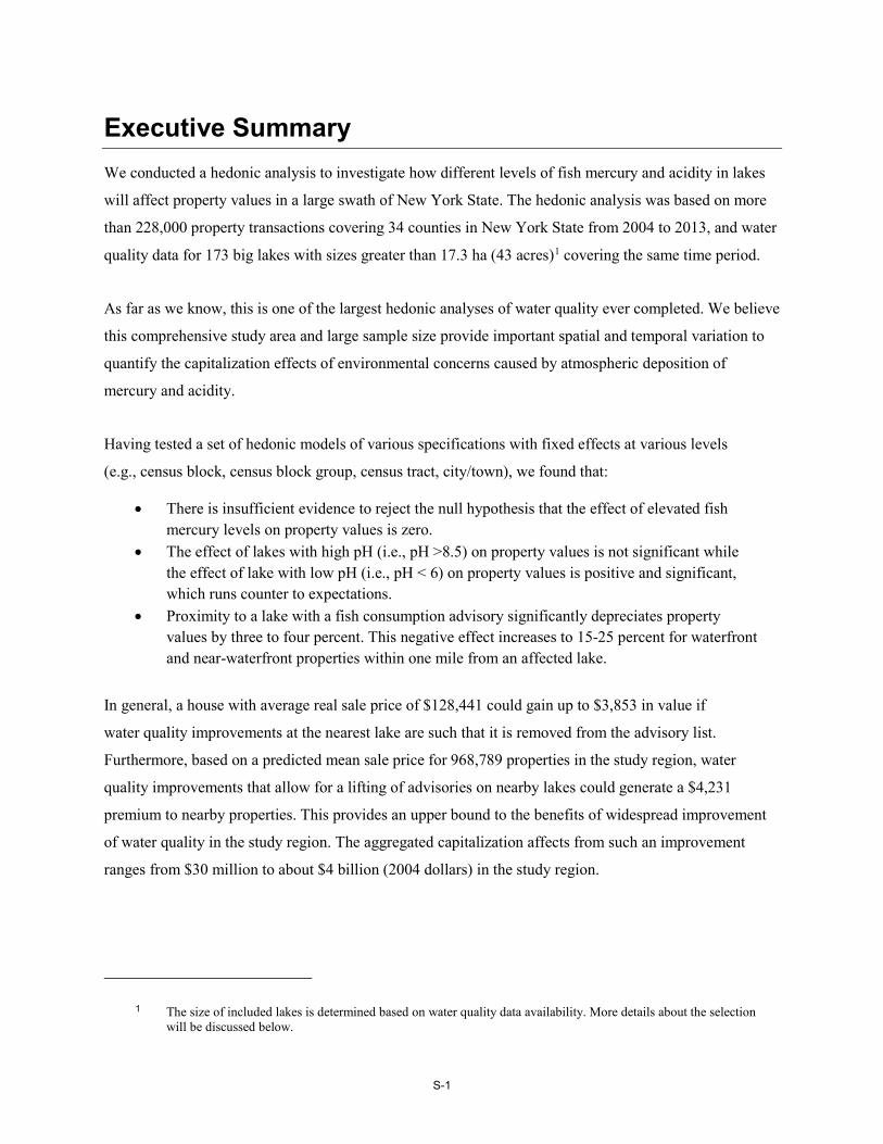
Executive Summary We conducted a hedonic analysis to investigate how different levels of fish mercury and acidity in lakes
will affect property values in a large swath of New York State. The hedonic analysis was based on more
than 228,000 property transactions covering 34 counties in New York State from 2004 to 2013, and water
quality data for 173 big lakes with sizes greater than 17.3 ha (43 acres)1 covering the same time period.
As far as we know, this is one of the largest hedonic analyses of water quality ever completed. We believe
this comprehensive study area and large sample size provide important spatial and temporal variation to
quantify the capitalization effects of environmental concerns caused by atmospheric deposition of
mercury and acidity.
Having tested a set of hedonic models of various specifications with fixed effects at various levels
(e.g., census block, census block group, census tract, city/town), we found that:
• There is insufficient evidence to reject the null hypothesis that the effect of elevated fish mercury levels on property values is zero.
• The effect of lakes with high pH (i.e., pH >8.5) on property values is not significant while the effect of lake with low pH (i.e., pH < 6) on property values is positive and significant, which runs counter to expectations.
• Proximity to a lake with a fish consumption advisory significantly depreciates property values by three to four percent. This negative effect increases to 15-25 percent for waterfront and near-waterfront properties within one mile from an affected lake.
In general, a house with average real sale price of $128,441 could gain up to $3,853 in value if
water quality improvements at the nearest lake are such that it is removed from the advisory list.
Furthermore, based on a predicted mean sale price for 968,789 properties in the study region, water
quality improvements that allow for a lifting of advisories on nearby lakes could generate a $4,231
premium to nearby properties. This provides an upper bound to the benefits of widespread improvement
of water quality in the study region. The aggregated capitalization affects from such an improvement
ranges from $30 million to about $4 billion (2004 dollars) in the study region.
1 The size of included lakes is determined based on water quality data availability. More details about the selection will be discussed below.

1
1 Introduction There are 17 major watersheds consisting of thousands of lakes, ponds, and reservoirs as well as tens of
thousands of miles of rivers and streams in New York State. These waterbodies often serve as drinking
water supplies for local communities, and as habitat for aquatic plants and animals. They also support a
wide range of human activities, including recreation, tourism, agriculture, fishing, power generation and
manufacturing. Unfortunately, those waterbodies are a primary medium through which mercury and acid
deposition impact ecosystems due to methylation and acidification in wetlands, lakes, and rivers (Driscoll
et al., 2003a; Krabbenhoft and Sunderland 2013).
In New York State, atmospheric deposition of mercury and acid rain rank among the top 10 most
prevalent causes/sources of water quality impact (DEC 2015). Within aquatic ecosystems, inorganic
mercury is transformed by certain bacteria to a special chemical form, methyl mercury, which is readily
bio-magnified through the trophic web, harming higher-level predators and leading to neurological
damage in humans (Meili 1997; Harris et al., 2003). Most people and wildlife at high trophic levels
are exposed to mercury by the consumption of methyl mercury contaminated fish. Meanwhile, abnormal
pH values likewise result in various adverse impacts on aquatic ecosystems. The Adirondack region of
New York State has historically received the highest rates of atmospheric inputs of acid deposition in the
United States (Driscoll et al., 2001). Most acid-sensitive lakes in New York State are in the Adirondack
region and are identified in New York's 1998 (and subsequent) Section 303(d) lists maintained pursuant
to the Clean Water Act (DEC 2014). The lake ecosystems are projected to be unable to achieve complete
chemical and biological recovery in the future (Zhou et al., 2015). Impaired water quality due to
atmospheric deposition of mercury and acid rain not only raises health concerns, but also causes
significant economic damage through the loss of valuable ecological services.
In order to address these environmental problems, several regulatory instruments have been proposed
and implemented in the United States. The United States acid rain program was enacted in 1990 as part
of the 1990 Clean Air Act Amendments (CAAA) and could be titled as the most successful “market-
based” environmental policy in the country. According to the EPA, more than 55 percent average
reductions have been achieved on wet deposition of sulfate across the eastern United States, over the
1989–1991 and 2009–2011 observation periods (EPA 2016). Though it may take longer than expected
for lakes to recover from acidification, significant decreases in acidification based on reductions in sulfur
deposition during 1992–2000 have been recorded in the Adirondack region (Driscoll et al., 2003b). The
estimated annual economic value under the Post-Clean Air Act scenario in the year 2020 will reach two

2
trillion dollars, which is mainly the consequence of significant reductions in air pollution related death
and illness, protecting the health of ecosystems, and better environmental conditions such as improved
agricultural yields and better visibility conditions (DeMocker 2003).
On the other hand, the 1990 Clean Air Act amendments give the EPA broad discretion in crafting
regulation to reduce power plant mercury emissions. Under section 112 of the CAAA, Congress identified
189 substances, including mercury as “hazardous air pollutants.” Since then, there have been dramatic
reductions in mercury emissions from most municipal waste combustors, medical waste incinerators,
and a number of other sources (Simonin et al., 2008). However, regulations on controlling emissions
of mercury and other common toxic air pollutants from power plants, the largest single source of
anthropogenic mercury emission in the United States (EPA 2011) have only recently been adopted.
In 2005, the EPA issued the Clean Air Mercury Rule (CAMR), limiting mercury emissions from new
and existing utilities. Similar to the acid rain program, this rule also included a cap-and-trade program
to reduce mercury emission in the nation within two phases. However, the U.S. Supreme Court vacated
this rule three years after its initialization. In 2011, the EPA announced the Mercury and Air Toxics
Standards (MATS) aiming at limiting mercury, acid gases, and other toxic pollution from power plants
exclusively. The U.S. Supreme Court again overturned MATS last year, declaring that the EPA should
take cost into consideration when finding it is “appropriate and necessary” to regulate electric utilities.
Eventually, in April 2016, the EPA provided final evidence including a consideration of cost and
maintained their determination in promoting MATS: “It is appropriate and necessary to set standards
for emissions of air toxics from coal- and oil- fired power plants.” Almost at the same time, the U.S.
Supreme Court changed its perspective and refused to stay MATS. Therefore, MATS becomes the first
standard in the U.S. for mercury emissions from power plants and is expected to lead to an extraordinary
nationwide reduction in the near future.
In crafting and evaluating policies to reduce atmospheric deposition of mercury and acidic compounds,
policy makers would be well-served to have information on the costs and benefits of these policies.
Since waterbodies, as an important part of the ecosystem, are the direct recipient of those adverse
depositions and are highly valued by the public (Keeler et al., 2012), measuring the economic values
of water quality and related ecosystem services is an important component to quantifying the benefits
of mitigating mercury and acidic emissions. Because there is no established market for surface water
quality, it is common to use a revealed preference approach, which relies on consumer behavior in related
markets to estimate the non-market benefits of improving environmental amenities. Housing markets are
a great example of a market where the composite goods prices are associated with their characteristics as

3
well as the services provided by their locations. With sufficient information on property transactions
and the market, the implicit price of one or several environmental amenities surrounding the houses
can be estimated.
Specifically, hedonic analysis uses regression techniques to estimate a hedonic price function, which
represents the impact of observable property characteristics, including environmental amenities and
spatial factors, on the equilibrium prices of parcels. By including observable characteristics, like lot
size, square footage, and some information about the buyer, including their mailing address, the method
will also be able to estimate how water quality factors impact the values of different types of homes in
different ways. This method is firstly proposed by Rosen (1974), which provides the framework for
estimating the dollar values of environmental amenities based on property values.
The idea of using the variation in housing prices to reflect the value of water quality can be traced
back to the 1960s. A study on 60 artificial lakes in Wisconsin, (David 1968) found that water quality
was positively associated with waterfront property values. This relationship between water quality and
property values was further explored and analyzed in a nationwide study concerning the potential
benefits of water pollution control on property values (Dornbusch and Barrager 1973). Subsequently,
more hedonic studies on water quality were performed in the spirit of Rosen's model (Epp and Al-Ani
1979; Leggett and Bockstael 2000; Gibbs et al., 2002; Poor et al., 2007; Phaneuf et al., 2008; Egan et al.,
2009; Guignet and Klemick 2015; Tuttle and Heintzelman 2015; Wolf and Klaiber 2016).
In general, a majority of hedonic studies on water quality agree that waterfront property owners capitalize
on the water quality of the adjacent lake/river as it increases their property value while degraded water
quality depreciates the value. In contrast to many previous hedonic studies, rather than clarity or other
more aggregated measures for water quality, this research includes specific measures, which have more
important ecosystem and human health implications (Michael et al., 1996; Boyle et al., 1999; Gibbs et al.,
2002; Walsh et al., 2011).

4
The two major objectives of this research are:
• Deploy the hedonic method to establish a link between lake water quality–specifically acidity (i.e., pH) and fish tissue Hg content, and property values–trying to reveal the dollar value of mercury pollution and acidification capitalized into people’s decisions in property transactions.
• Use results of hedonic property value analysis together with model forecasts of future environmental conditions under various policy scenarios to estimate future changes in property values from water quality changes.2
2 Since the actual fish mercury level is not found to affect property values, we perform predictions based on hypothetical policy scenarios to remove fish advisories on lakes. More details about prediction and results will be discussed below.

5
2 Study Area & Data
2.1 Study Area
The study area of this research covers 34 counties of New York State3as shown in Figure 3-1. The
reasons for choosing those counties are generally three-fold. First, the lakes in these counties are the
ones most heavily impacted by mercury deposition and acid rain in the State. The NYS section 303(d)
list of impaired waters is a list of waters that fail to meet certain water criteria, can no longer support
appropriate uses, and may require development of a Total Maximum Daily Load (TMDL). Major lakes
in our study area can be found on this list as impaired waters. Second, water quality data and transaction
data for those counties are relatively comprehensive. In order to achieve sufficient variation in water
quality, we need to confine our study area to regions with the most available data. Last, many lakes
within the selected counties, especially those in the Adirondack Park and Finger Lakes Region, are
important destinations for fishing and recreation in NYS.
3 Those 34 counties include: Albany, Cayuga, Chenango, Clinton, Columbia, Cortland, Essex, Franklin, Fulton, Hamilton, Herkimer, Jefferson, Lewis, Livingston, Madison, Montgomery, Oneida, Onondaga, Ontario, Oswego, Otsego, Rensselaer, Saratoga, Schenectady, Schoharie, Schuyler, Seneca, St. Lawrence, Steuben, Tompkins, Warren, Washington, Wyoming, Yates.

6
Figure 2-1. Map of Study Area
2.2 Transaction Data
We collected and compiled 332,652 real residential property transactions from 2004–2013 in the
34 counties. The New York State Office of Real Property Taxation Services provided the real estate
transactions dataset as well as the detailed parcel and property characteristics of all transactions. In
the data cleaning stage, transaction observations that have incomplete and abnormal records – such
as, number of bedrooms less than one, number of stories less than one, etc. – were cleaned out. Outlier
observations, such as sale price lower than $10,000 or living area less than 100 square feet were discarded
as well. We also dropped out transactions data with unidentified/incomplete address information. Finally,
the transaction dataset contains 218,832 real property sales to be used for hedonic analysis.

7
We projected each transacted parcel-on-parcel reference shapefile via ArcGIS (v13.1). We measured
the Euclidean distance between each parcel centroid to environmental and cultural amenities, including
population centers, hospitals, public schools, lakes and others. This spatial information is integrated into
the hedonic analysis model to carefully control locational effects on property values. In our analysis,
we focused on large lakes that serve for multiple water-based recreational activities such as fishing,
boating and swimming. We consider that both waterfront and non-waterfront property owners are
likely to care about the water quality of those lakes. We therefore link every parcel in our database to
the nearest lake equal to, or larger than, 17 ha (43 acres). This lake size threshold was determined based
on the 25th percentile of the size of all lakes with water quality data (either acidity or fish mercury, or
both). This cut-off is a balance between taking advantage of as much available water quality data and
impeding the noise brought by lakes with unknown information. This way, there are 629 lakes included
in the hedonic analysis, with 173 lakes that have water quality information4. With this specification,
we made an assumption that those specific sized lakes are major water recreation destinations for nearby
property owners. The water quality of those lakes would therefore influence consumer decisions related
to both recreation and home purchases.
In addition, all transaction data were deflated to the base year 2004 using the quarterly house price index
(HPI) constructed by the Federal Housing Finance Agency. Our study area covers seven metropolitan
statistical areas (MSA)5. If available, we used specific HPI for major MSA otherwise, the HPI for non-
metropolitan New York State was used. The log form of deflated sale price was used as the dependent
variable in the hedonic model.
4 We also tried setting the lake size threshold to 15 acres (10 percentile) and to 135 acres (50 percentile). The hedonic analysis results are not substantially different from those shown in this report using 43 acres. In this final report, we only report results based on 43 acres threshold. We also excluded water quality data for Lake Champlain and Lake Ontario. We mark those two lakes as data “unknown” in the later hedonic analysis since we consider that water quality of those huge lakes is hard to be described with just a few discrete observations.
5 Those seven MSA are: Albany-Schenectady-Troy; Ithaca; Syracuse; Watertown-Fort Drum; Glens Falls; Rochester; Utica-Rome.
8
2.3 Water Quality Data
2.3.1 Fish Mercury Data
Fish mercury data used in our hedonic analysis mainly comes from the fish mercury database maintained
by the Division of Fish, Wildlife and Marine Resources of New York State Department of Environmental
Conservation (DEC). The DEC started monitoring the mercury concentration in fish tissue in the late
1960s. Continued monitoring programs have tracked trends in fish mercury levels in NYS since then
(Howard Simonin et al., 2008). More recently, several independent mercury monitoring programs are
active for research purposes6. This database primarily stores contaminant results for samples taken in
NYS. There are results from other states as well, mostly from marine waters. Most samples are from fish,
but aquatic vertebrates and terrestrial animals are also present. The database contains nearly all analyses
done by or for the Division of Fish, Wildlife and Marine Resources’ contaminant monitoring program
since about 1970 to 2015. In addition, we also include fish mercury monitoring data from 2008 to 2012
by the Adirondack Lakes Survey Cooperation, a non-profit-organization. This monitoring project
collected approximately 600 fish samples, covering 36 lakes within the Adirondack region. All fish
samples were analyzed for total mercury concentration while a few samples were tested for methyl
mercury concentration.
Following the scientific literature on mercury contamination (Simonin et al., 2009; Yu et al., 2011;
Wathen et al., 2015), the total mercury concentration in fish tissue was used as the mercury pollution
indicator for lakes. Though only methyl mercury poses a threat to human beings, data for methyl mercury
in fish body are normally scarce compared to data of total mercury concentration. Fortunately, methyl
mercury concentrations in fish muscle are directly proportional to total mercury concentrations, but
the ratio varies by abiotic factors of different locations and by fish species (Kannan et al., 1998). It is
reported that methyl mercury accounts for 64-100 percent of the total mercury in fish body (Agah et al.,
2007; EPA 2011). The usage of total fish mercury directly instead of converting it into methyl mercury
in our analysis could be regarded as a worst-case scenario approach to estimate the average fish mercury
pollution in a lake.
6 From 2001–2003, DEC led a project investigating the mercury and organic chemicals in fish from the New York City reservoir system. In 2006, DEC reported another project studying the total and methyl-mercury in the Never-sink reservoir watershed. Furthermore, the Biodiversity Research Institute (BRI) has conducted a project assessing mercury concentration in loons and prey fish at 44 lakes in Adirondack region during 2003 to 2004. NYSERDA funded another extensive fish mercury monitoring project during 2003–2007, analyzing 2605 individual fish mercury samples from 131 lakes in New York State.

9
In total, we initially compiled 26,642 fish mercury data points from these two data sources. We
filtered out fish observations with incomplete information, such as missing fish length or if the sampling
coordinate is unidentified or incorrect. We also dropped observations where fish mercury is reported
to be negative. Since we only focus on lakes in this research, any fish mercury observations from rivers,
streams, creeks/brooks, and canals are dropped out as well. Furthermore, we dropped observations which
is the only observation for certain species and rename species with few observations (<5) to species
alike7. Finally, we have 7,563 fish observations covering 207 lakes across the State from 1970 to 2015
in the ready-to-use dataset for fish mercury standardization.
In addition, we introduced fish advisory information into hedonic analysis. According to the EPA:
“A fish consumption advisory is a recommendation to limit or avoid eating certain species of fish or
shellfish caught from specific water bodies or types of water bodies (e.g., lakes, rivers or coastal waters)
due to chemical contamination.” Fish advisory thus becomes the direct path from which the general
public retrieve information about mercury pollution in the lakes near to them. Incorporating fish advisory
information allows us to identify how being proximate to a lake with fish advisory affects property
values. More details about this variable and how it works in the hedonic model and predictions will
be discussed in next sections.
2.3.2 Fish Mercury Standardization
Since fish mercury data are derived from different monitoring programs, there are differences in the
characteristics of fish samples collected over time and across different lakes which presents a challenge in
comparing pollution levels across lakes. Without standardizing raw fish mercury data, the actual mercury
pollution level of different lakes may be falsely interpreted due to variations in sample characteristics,
such as species, size, age, etc. (Wente 2004). For example, a larger fish (e.g., Walleye) caught in Lake A
may contain higher mercury than a smaller fish (e.g., yellow perch) taken from Lake B. However, based
on those two fish samples, it would be inappropriate to conclude that Lake A is more polluted than Lake
B since the higher mercury concentration of the larger fish could be the consequence of its higher trophic
7 We dropped the only observation whose species named as “PNTL” and re-classify five observations whose species are “MUSK (Musky)” and “TML (Tiger Muskelluge)” as “NOP (Northern Pike).”
10
status or longevity. Environmental scientists have proposed various methods (Somers and Jackson 1993;
Parks et al., 1994; Meili 1997; Tremblay et al., 1998; Sonesten 2003; Wente 2004; Money et al., 2011)
and applied them in numerous regional or nationwide fish mercury related studies (Lockhart et al., 2004;
Kamman et al., 2005; Driscoll et al., 2007; Evers et al., 2007; Melwani et al., 2009; Simonin et al., 2009;
Gandhi et al., 2014; Åkerblom et al., 2014; Wathen et al., 2015).
Each standardization method has its own advantages and disadvantages in interpreting fish mercury
monitoring data. Surprisingly, there has been minimal effort to systematically evaluate the relative
performance of these methods. Since accuracy of comparable fish mercury levels will dictate the results
of hedonic analysis, we choose four widely used standardization methods to process our data. We then
applied hedonic analysis based on the results of those four standardization methods to test the sensitivity
of those different methods in hedonic analysis. More details about the standardization methods are
discussed in Methods section.
2.3.3 Lake Acidity Data
Similar to many other hedonic analyses (Epp and Al-Ani 1979; Netusil et al., 2014; Tuttle and
Heintzelman 2015), pH is used as an indicator for the acidity level of lakes in this study. It is the
most frequently measured water chemical parameter and reduced pH is one of the most important
impacts of acidic deposition on watersheds(Driscoll et al., 2003a). There are many water quality
monitoring programs in NYS that track acidity. In order to maintain the consistency and integrity
of our dataset, we only employ data from programs that have the most comprehensive and complete
monitoring data over time. For our hedonic analysis, we include pH data from three different monitoring
programs: (1) the New York Citizens Statewide Lake Assessment Program (CSLAP) conducted by DEC,
(2) Adirondack Long Term Monitoring (ALTM) program administered by the Adirondack Lake Survey
Corporation and the Temporally Integrated Monitoring of Ecosystems (TIME) conducted by the EPA
since 1991 as part of EPA Environmental Monitoring and Assessment Program. We used the arithmetic
mean of monthly observed pH to indicate the average yearly acidity level of a lake. In summary, we
obtained 3,173 yearly acidity observations for 232 lakes from 1986–2012 within our study area.
Table 2-1 is a summary of data sources for this research.

11
Table 2-1. Summary of Data Sources
Data Description Time Frame Source 1 Fixed effect (e.g., census block/block
group/tract, town city) Reference Shapefile 2015 U.S. Census Bureau
2 Amenities Reference Shapefile (e.g., Public facilities, population centers, etc.)
various New York State GIS Clearinghouse
3 Water Body Reference Shapefile 2012 National Hydrologic Database (NHDplus)
4 Parcel Shapefile 2012-2013 Individual counties 5 Parcel Sale Data & Characteristics 2004-2013 NYSORPTS Fish Tissue Mercury Data 1970-2015 Division of Fish, Wildlife and
Marine Resources(NYSDEC) Adirondack Lakes Survey
Cooperation 6 Acidity Data 1986-2012 NYSDEC
Adirondack Lake Survey Corporation U.S. EPA
7 Fish Advisory Reference Shapefile and Other Information
2010 U.S. EPA Office of Water (OW) New York State Department of
Health (NYSDOH)

12
3 Methods
3.1 Hedonic Analysis Model
3.1.1 Empirical Model
The hedonic method generally involves two stages. The first stage is to estimate the hedonic price
function by regressing house prices on attributes using an econometric model, then the marginal implicit
prices of the attributes can be recovered from the estimated coefficients. The second stage aims to derive
the demand function for attributes based on the results of first stage. Most hedonic studies, including this
one, focus on the first stage hedonic estimation due to its well-defined framework and the challenges
associated with estimating the second stage with confidence.
The general form of the hedonic model applied in this study is:
Equation 1. 𝐥𝐥𝐥𝐥(𝑷𝑷𝑷𝑷𝑷𝑷𝑷𝑷𝑷𝑷) = 𝒇𝒇(𝑺𝑺,𝑳𝑳,𝑬𝑬)
where Price is the real transaction price, S is the structural characteristics, L is the locational
characteristics, and E indicates environmental characteristics.
Given that the form of the econometric model was not explicitly defined in Rosen's paper, like other
studies, we employ a standard semi-log specification for our regression model (Kuminoff et al., 2010).
When constructing the econometric model, several potential econometric challenges and issues that
may lead to biased estimates need to be addressed. These challenges include arbitrary functional form,
omitted variable bias, endogeneity, spatial dependence and autocorrelation, heteroscedasticity, and
multicollinearity. In hedonic studies on water issues, the most discussed common problem is omitted
variable bias (Tuttle and Heintzelman 2015). Econometricians may fail to include important
characteristics that are correlated to other independent variables and important to home buyers,
which then bias the remaining estimated coefficients. The “emitter effect” described by (Leggett
and Bockstael 2000) is an example of this problem. In the case where home owners live near pollution
emitters and variables indicating the proximity to those emitters are missing, the seemingly correct and
significant impacts of water quality on house values suggested by regression results may actually be the
consequence of other nuisance, such as noise or odors, brought by pollution emitters.

13
Knowing that omitted variables bias exists in our model since it is impossible to have information on all
house price related characteristics, therefore we used spatial fixed effects to absorb the price effects of
spatially clustered omitted variables. We incorporated a variety of fixed effect levels into our hedonic
model in order to balance the competing goals of reducing omitted variables bias (done by using smaller
scale fixed effects) and maintaining sufficient variation in our variables of interest to allow for proper
identification. The introduction of fixed effects is important in terms of ensuring the accuracy of model
estimation. In addition, in order to dampen the spatial autocorrelation and heteroscedasticity, we allow
the clustering of error terms for parcels within each fixed effects group, but enforce the error terms to be
independent across the groups.
The specific model applied in this study can be written as:
Equation 2. 𝐥𝐥𝐥𝐥 (𝑷𝑷𝑷𝑷𝑷𝑷𝑷𝑷𝑷𝑷)𝑷𝑷𝒊𝒊𝒊𝒊 = 𝜷𝜷𝟎𝟎 + 𝜷𝜷𝟏𝟏𝑺𝑺𝑷𝑷𝒊𝒊 + 𝜷𝜷𝟐𝟐𝑿𝑿𝒊𝒊 + 𝜷𝜷𝟑𝟑𝑳𝑳𝒊𝒊 + 𝜷𝜷𝟒𝟒𝒑𝒑𝒑𝒑𝑷𝑷𝒊𝒊 + 𝜷𝜷𝟓𝟓𝑭𝑭𝑷𝑷𝑭𝑭𝑭𝑭𝒑𝒑𝑭𝑭𝑷𝑷𝒊𝒊 + 𝜼𝜼𝒊𝒊𝒊𝒊 + 𝝐𝝐𝑷𝑷𝒊𝒊
where ln (𝑃𝑃𝑃𝑃𝑃𝑃𝑃𝑃𝑃𝑃)𝑖𝑖𝑖𝑖𝑖𝑖 represents the price of the property i in the fixed effects group j at time t; 𝑆𝑆𝑖𝑖𝑖𝑖 stands
for characteristics (e.g., number of bedrooms, living space, etc.) of property i in group j; 𝑋𝑋𝑖𝑖 represents
a set of time series dummy variables for the month and year of sale; 𝐿𝐿𝑖𝑖 is the fixed group effects(e.g.,
census block, census block group, etc.); 𝑝𝑝𝑝𝑝𝑖𝑖𝑖𝑖 and 𝐹𝐹𝑃𝑃𝐹𝐹ℎ𝑝𝑝𝐻𝐻𝑖𝑖𝑖𝑖 are categorical variables for t year average
pH (i.e., High, Normal, Low, Unknown) and for average fish mercury level (Unsafe, Safe, Unknown)
in the nearest large lake connected to property i, therefore, 𝛽𝛽4 and 𝛽𝛽5 are parameters we are interested
in; lastly, 𝜂𝜂𝑖𝑖𝑖𝑖 and 𝜖𝜖𝑖𝑖𝑖𝑖 are fixed effects group error and individual error respectively.
3.1.2 Specification of Variables
3.1.2.1 Fish Mercury
Average people's perceptions of water quality are general rather than quantitative. Therefore, it may
not be appropriate to use continuous scientific measures in hedonic analysis and estimate the implicit
price for water quality based on a continuous scale. We transformed the continuous water quality data
into categorical variables. The 0.3 parts per million (ppm) human health criterion for methyl mercury in
fish tissue established by the EPA and the U.S. Food and Drug Administration (FDA) is the maximum
advisable concentration of methyl mercury in fish body to protect consumers (Driscoll, C.T. et al., 2007).
We follow these criteria and sort the yearly average fish mercury data into three categories: safe (lesser
or equal to 0.3 ppm), unsafe (greater than 0.3), and unknown (all lakes that have not been sampled).
The safe level was used as the reference level in hedonic model (the omitted category). In the following
section, fish mercury levels of a lake mean the yearly average fish mercury level of that lake.

14
3.1.2.2 Acidity
The lake acidity level was captured using the annual average pH of lakes. Though pH readings could
not be observed by home owners and lake users directly, abnormal pH values could noticeably affect the
ecosystem, reducing species diversity and abundance of aquatic life (Driscoll et al., 2003a). Scientifically,
pH is a numeric scale for acidity. In natural conditions, a lake’s pH measure falling between 6.5 and 8 is
considered normal. Lakes with pH values that are either too low or too high are all regarded as impaired.
This unique characteristic of pH suggests that it is inappropriate to use continuous pH readings in hedonic
models due to the ambiguity in interpretation. As a result, most existing studies transform continuous pH
readings into dummy variables distinguishing acid-stressed lakes from others (i.e., dummy variable equals
to zero if pH was 5.5 or lower, otherwise equal to one) (Epp and Al-Ani 1979). In our dataset, the annual
pH values range from 4.21 to 9.31. Lakes with pH lower than 6.5 were coded as Low and those with pH
greater than 8 are coded as High, otherwise, as Normal (>= 6.5 and <=8). Lakes without pH readings are
marked as Unknown. Therefore, in the following section, the pH level of a lake means the yearly average
pH level of that lake.
In addition, for all sampled lakes, pH and fish mercury data measured in the same year of sale are used.
When water quality measurements corresponding to the year of sale are not available, the measurement
taken closest to the time of sale is used instead. Water quality variables for lakes not sampled are marked
as unknown. We match the transaction data with water quality data in this way based on the assumption
that water quality, especially yearly average lake pH and fish mercury, fluctuate slightly year by year. In
fact, it may take many years for a lake which has already been polluted to recover, by itself, to a healthy
state. Once polluted, some lakes will never be able to recover to its healthy state.
3.1.2.3 Fish Advisory
We incorporate fish advisory information in the hedonic analysis by using a dummy variable to identify
whether a lake in our study area has been designated with a fish advisory. Specifically, lakes with an
active individual fish advisory are coded as one while all others without advisories are coded zero.
We identified the location of fish advisory events following the instructions of the EPA Office of Water
(OW)8. There are 60 lakes that have been assigned fish advisories due to mercury pollution exclusively.
8 The Fish Consumption Advisories and Fish Tissue Sampling Stations NHDPlus Indexed Datasets. The detailed dataset and shapefile are available for downloading using the EPA “Clip N Ship Application”: https://edg.epa.gov/clipship/. The specific information on fish advisory can be found on “EPA NLFA Technical Advisories Search” website: https://fishadviFsoryonline.epa.gov/Advisories.aspx

15
However, in the hedonic model we incorporate fish advisory information regardless of the type of
pollutants (e.g., PCBs, Chlordane, Dioxin, etc.) and fish species based on the assumption that the effects
of various fish advisories have a similar impact on property values9. In total, according to the shapefile
provided by the OW, there are 556 lakes among our 629 lakes (area greater than 17 ha) that have active
individual fish advisories. We believe incorporating this variable into the hedonic analysis model is
important and necessary since it allows us to identify how assigning a fish advisory to a lake affects
property values nearby. In addition, a fish advisory is the direct information obtained and understood
by property owners and could be influential in the house purchasing process.
3.1.2.4 Locational Variables
The locational characteristics of each parcel include distance between the centroid of each parcel to the
nearest facilities, including a public hospital, school, university, bus/rail station and population center.
We also include the size of the lake in our model. As to measuring the effects provided by nearest lake,
a non-linear function of distance to the nearest waterbody to proxy for the ecosystem service effects
was proposed and applied in hedonic analysis (Phaneuf et al., 2008). We follow the same convention
to describe the fact that the amenity effect is diminishing as distance becomes larger. The variable
lakeproxy is created by using the function below:
Equation 3. 𝐥𝐥𝐥𝐥𝐥𝐥𝐥𝐥𝐥𝐥𝐥𝐥𝐥𝐥𝐥𝐥𝐥𝐥 = 𝐦𝐦𝐥𝐥𝐥𝐥 �𝟏𝟏 − � 𝒅𝒅𝒅𝒅𝒎𝒎𝒎𝒎𝒎𝒎
�𝟏𝟏𝟐𝟐 ,𝟎𝟎�
where d is distance between parcel to included lake and dmax is the threshold point indicating the amenity
effect diminishes to zero. Though setting the value for dmax is somewhat arbitrary, we set dmax to one mile
in our application based on the finding of previous study (Walsh 2009). This variable is between zero and
one and is convex.
9 We first incorporated fish advisory information due to mercury exclusively and found that it was not significantly related to property values.

16
It is worth noting that there are more than 4,000 waterbodies (e.g., lakes, ponds, reservoir, etc) identified
within the study area, most of which are quite small and do not have water quality data. As previously
mentioned, we linked each parcel in our database to the nearest lake equal to, or bigger than, 17 ha
(43 acres). However, one concern remains in using this approach: households presumably care about
the water quality of those waterbodies in addition to the larger ones which we are able to measure. We
partially control for this situation by creating a dummy variable, lake_tag, indicating the existence of at
least one small lake between the parcel and the nearest threshold lake.
3.1.2.5 House Structural Variables
House structural characteristics include the number of bedrooms, kitchens, full and half bathrooms, and
fireplaces. Other amenities, such as a finished basement, the capacity of basement and garage, and central
air-conditioning are also included. Age of building and log form of square foot of living area are also
considered. In addition, all included parcels are classified into seven groups: mobile, residential multi-
purpose, residential, rural residence with acreage, seasonal residence, estate, and other. Each parcel is also
graded on condition into five levels: bad (E), fair (D), average (C), good (B) and excellent (A), as defined
by assessment records.
3.2 Fish Mercury Standardization
In the final ready-to-use fish mercury dataset, there are 7,563 observations of 23 species covering
207 lakes and 45 years (1970–2015). The objective of standardization is to find the most accurate and
comparable fish mercury level for each sampling event (i.e., combination of sampling site and year). We
deployed four different methods to standardize the fish mercury data with consideration of heterogeneity
in fish length, species, sampling sites, and time. After standardization, the annual arithmetic average of
fish mercury concentration was calculated as fish mercury level for each lake. We conducted hedonic
analysis based on standardized fish mercury level derived by those four models individually to check the
sensitivity of hedonic analysis. Results of those analyses will be discussed thoroughly in next section.
Specifically, those four standardization methods are: Analysis of Covariance (ANCOVA) (Kamman et
al., 2005); Mixed-effect model (Eagles-Smith et al., 2016); National Descriptive Model for Mercury in
Fish (NDMMF)(Wente 2004) and Empirical Fish Mercury Transfer Function suggested by the United
Nations Economic Commission for Europe (CLRTAP 2004). All analysis in this part was completed by
R statistical program (R Development Core Team 2008).
17
3.2.1 ANCOVA Model (Fixed-Effect Model)
Analysis of Covariance (ANCOVA) is an appealing approach integrating not only information of fish
characteristics but factors vary substantially during different sampling events (i.e., sampling site and
sampling year) as well. Since the model focuses on all main effect of all variables, it is also called
Fixed Effect model10. The ANCOVA model we used is shown as below:
Equation 4. 𝐥𝐥𝐥𝐥𝐥𝐥 (𝑭𝑭𝑷𝑷𝑭𝑭𝑭𝑭𝒑𝒑𝑭𝑭)𝑷𝑷𝒊𝒊𝒊𝒊 = 𝜷𝜷𝟎𝟎 + 𝜷𝜷𝟏𝟏𝐥𝐥𝐥𝐥𝐥𝐥 (𝑳𝑳𝑷𝑷𝑳𝑳𝑭𝑭𝒊𝒊𝑭𝑭)𝑷𝑷 + 𝜷𝜷𝟐𝟐𝑺𝑺𝒑𝒑𝑷𝑷𝑷𝑷𝑷𝑷𝑷𝑷𝑭𝑭𝑷𝑷 + 𝜷𝜷𝟑𝟑𝑺𝑺𝑷𝑷𝒊𝒊𝑷𝑷𝒊𝒊 + 𝜷𝜷𝟒𝟒𝒀𝒀𝑷𝑷𝒎𝒎𝑷𝑷𝒊𝒊 + 𝝐𝝐𝑷𝑷𝒊𝒊
where Length is continuous variable while Species is categorical variable indicating species; Site and
Year are dummy variables indicating sampling site and year, 𝜖𝜖𝑖𝑖𝑖𝑖 is the error term. The estimate mean
fish mercury value based on yellow perch of 234 mm (i.e., median length of pooled observations) for
each sampling event were used for hedonic analysis.
3.2.2 Mixed-Effect Model
Though fish length was found to be strongly correlated with fish mercury concentration (R.S. Thorpe
1976; Gewurtz et al., 2011), a bivariate model that uses fish length as the only explanatory variable
(Simonin et al., 2009) completely pools the entire dataset and ignores any variations in average fish
mercury level between species and sampling events. On the other hand, the ANCOVA model focuses
on the main effect of each explanatory variable. It does not pool the data entirely and therefore bias the
results for species or sampling events with few observations. Mixed-effect model, however, provides a
more flexible approach to describe data by partial pooling the entire dataset: when observations are scarce
in certain groups (e.g., species group), the model will get more smooth estimates similar to the overall
mean level; when observations are rich in other groups, the model will generate estimates close to the
group mean level.
10 There are lots of discrepancies in describing “fixed effect” and “random effect”. We avoid using those terms in this report for reducing ambiguity.

18
Similar to (Eagles-Smith et al., 2016), the mixed-effect model used here takes fish length as the single
fixed covariate, and sampling site, species, and an interaction term of species and length as random
effects. In order to account for the variations of sampling years, we also include year as another random
effect term in this model. The model was run using the lme4 package of R (Bates et al., 2014). The
estimate mean fish mercury value based on yellow perch of 234 mm for each sampling event were
used for hedonic analysis.
3.2.3 National Descriptive Model for Mercury in Fish (NDMMF)
The National Descriptive Model for Mercury in Fish was firstly proposed in (Wente 2004) and officially
recommended by USGS. It takes the spatial and temporal trends of fish mercury level into consideration
and has a parsimonious specification. Wente (2004) described that this model fit the fish mercury data
from National Listing of Fish and Wildlife Advisories database very well with a pseudo-R squared of
0.82. It is also found that this model performs well on standardizing and predicting fish mercury of yellow
perch and walleye in Ontario Lake, Canada (DeLong 2012). The specific form of model is shown as:
Equation 5.
where C𝑖𝑖𝑖𝑖𝑖𝑖 is the fish mercury concentration from ith sample of the jth sampling event (i.e., a collection
of samples from a specific site and date) for the kth species and cut combination (e.g., skin-off fillet);
α𝑖𝑖 is a set of parameters relating variation in fish mercury concentration to fish length for each of m
species and cut combinations of fish11; Length𝑖𝑖𝑖𝑖𝑖𝑖 is the length of the ith sample of the jth sampling event
11 It is worth mentioning that the α𝑖𝑖 term only indicates m species in our model rather than species and cut combination since, in our fish mercury dataset, the fish cut is unknown. We assume that all fish samples are prepared using identical fish cut.

19
for the kth species; β𝑖𝑖 is a set of parameters describing variation in fish mercury concentration among each
of n sampling events; ε𝑖𝑖𝑖𝑖𝑖𝑖 is an error term for the ith sample of the jth sampling event for the kth species; k𝑙𝑙
is the value of k for the lth observation; and j𝑙𝑙 is the value of j for the lth observation. The estimate mean
fish mercury values based on yellow perch of 234 mm for each sampling event were used for hedonic
analysis.
3.2.4 Empirical Fish Mercury Transfer Function
Besides regression-based standardization methods, some research applied empirical transforming model
to convert fish mercury with heterogeneous sampling characteristics into one comparable species (Meili
1997; Depew et al., 2013; Åkerblom et al., 2014). One example is introduced by the United Nations
Economic Commission for Europe (CLRTAP 2004):
Equation 6. 𝒑𝒑𝑭𝑭𝑭𝑭𝒊𝒊𝒅𝒅 = 𝒑𝒑𝑭𝑭𝒐𝒐𝒐𝒐𝑭𝑭
�𝒇𝒇𝒑𝒑𝑭𝑭𝒀𝒀+ 𝒇𝒇𝒑𝒑𝑭𝑭𝑯𝑯𝑯𝑯𝟐𝟐𝟑𝟑�
where 𝑝𝑝𝐻𝐻𝑠𝑠𝑖𝑖𝑠𝑠 is the standardized mercury concentration, 𝑝𝑝𝐻𝐻𝑜𝑜𝑜𝑜𝑠𝑠 is the observed mercury concentration;
𝑓𝑓𝐻𝐻𝐻𝐻𝐻𝐻 is a parameter representing the concentration ratio between newly hatched young fish and 1-kg
pike, and 𝑓𝑓𝐻𝐻𝐻𝐻𝐻𝐻 is a species-specific empirical coefficient; W is the wet weight of fish sample. According
to (Åkerblom et al., 2014), parameters were set to default values: 𝑓𝑓𝐻𝐻𝐻𝐻𝐻𝐻 to 0.13 and 𝑓𝑓𝐻𝐻𝐻𝐻𝐻𝐻 0.87 for pike,
1.65 for perch, and 1 for other species. Therefore, observed individual Hg concentrations were
standardized correspondently to a 1-kg pike in the same lake12.
12 We were unable to transfer individual fish mercury to yellow perch due to insufficient information for transfer parameters. However, the 1-kg pike standardized results make no difference from other standardize methods in hedonic analysis: there effects of fish mercury level on property values is nominal.

20
4 Hedonic Analysis Results and Discussion
4.1 Sensitivity Analysis of hedonic analysis
We deployed several validation approaches and statistics for the performance test. The Coefficient of
Determination (R squared, denoted as R2 or r2) of a regression model will be used to measure how well
data will fit the regression model. For a regression model, the R square indicates the ratio of variance
explained by the model to the total variation in the dependent variable. Mean Absolute Error (MAE)
represents the average absolute deviation of predicted values with respect to the observed ones. It is
an unambiguous measure of average error magnitude. Generally, the smaller MAE is, the better a
standardizing method performs. Root Mean Square Error (RMSE) is used for measuring the quantity
of accuracy of this regression model. Similarly, the smaller RMSE is, the better a standardizing method
performs. The Akaike information criterion (AIC) (Arlot et al., 2010) is a measure of the relative quality
of the full and reduced forms of a regression model for a given set of data. Among a set of candidate
models for the data, the most preferred model is the one with lowest AIC value. Different from r square,
AIC rewards goodness of fit, but penalizes the number of variables included in the model. In addition,
Bayesian Information Criterion (BIC) is based, in part, on the likelihood function and used in similar
convention as AIC. Table 4-1 shows a summary of statistical performance of those four methods.
Table 4-1. Summary of Statistical Performance of Four Fish Standardization Methods
Methods Adj. R square AIC BIC RMSE MAE 1 VA(Fixed-Effect) 0.8618 7075 8926 0.6683 0.4824 2 Mixed-Effect NA -10195 -10146 0.0947 0.0700 3 NDMMF 0.9961 6581 9069 0.1869 0.1097 4 Transfer Function NA NA NA 0.3489 0.2318
* NA indicates statistics are not available.
Four models are all used to describe our fish mercury data with consideration of temporal and spatial
trends. Those statistics illustrate how well those models not only describe a real dataset, but also, predict
new observations. According to Table 4-1, it is easy to conclude that the mixed-effect model is superior
among those four methods in terms of relative low RMSE and MAE, and low AIC and BIC. Therefore,
in the further hedonic analysis with various fixed-effect scenarios, we only used the fish mercury
standardized by mixed-effect model. However, for the sensitivity analysis, we conducted hedonic
analysis based on fish mercury calibrated by all four models individually and evaluate the differences
in estimating the effect of fish mercury on property values.

21
Table 4-2. Hedonic Analysis Results Based on Four Fish Mercury Standardization Methods
(1) (2) (3) (4)
Mixed-Effect ANOVA NDMMF Transfer Function
Lakeproxy 0.683*** 0.683*** 0.683*** 0.686*** (0.0317) (0.0317) (0.0317) (0.0318)
Fish Advisory -0.0294** -0.0295** -0.0292** -0.0225 (0.0147) (0.0147) (0.0147) (0.0148)
Lake_tag 0.0168** 0.0168** 0.0168** 0.0168** (0.00771) (0.00770) (0.00770) (0.00771)
Fish Hg (Unknown) -0.0222 (0.0137)
-0.0220 (0.0136)
-0.0236* (0.0136)
0.00814 (0.0121)
Unsafe Fish Hg (>0.3 ppm)
-0.00390 (0.0239)
-0.00234 (0.0241)
-0.0138 (0.0241)
0.00466 (0.00758)
Constant 7.542*** 7.542*** 7.545*** 7.511*** (0.271) (0.270) (0.271) (0.273)
FE-groups 2668 2668 2668 2668 Year/Monthly FE YES YES YES YES
R-squared 0.403 0.403 0.403 0.403 Observations 218832 218832 218832 218832 * p<0.10, ** p<0.05, *** p<0.01 Standard errors (SEs) in parentheses. SEs have been clustered at the FE levels respectively Fixed-effect level: census block group
Table 4-2 shows the regression results for major variables based on those four standardization models.
The full regression results are available in the appendix. The hedonic analysis was performed using
census block group as fixed-effect level. Disproxy and Lake_tag are both positive significant across
four models, these consistent results indicate that the closer a property is to a lake, the higher the value,
and a smaller lake within the distance to the interested big lake also is of value to homeowners, which
proves our hypothesis. As to the estimation on fish mercury categorical variables, the regression results
are consistent showing that, ceteris paribus, unsafe fish mercury levels of lakes have nominal effects on
property values compared to lakes with safe fish mercury levels (<=0.3 ppm). The estimation for mercury
unknown category is also insignificant except for model 3 (NDMMF). The sensitivity test confirms
that the four standardization methods do not significantly alter the results of hedonic analysis. This is
reasonable since we used categorical variables rather than using continuous variables for fish mercury
directly. The standard error of each standardization method are considered trivial in determining the
category that a lake should be assigned to.

22
4.2 Hedonic Analysis
We performed hedonic analysis using basic OLS model with fixed effect on different levels: census
block, census block group, census tract, and city-town group. The standardized mercury data prepared
by the mixed effect model and acidity data were used for those hedonic analysis. Table 4-3 is a summary
of primary variables of hedonic analysis. Full regression results can be found in the appendix.
Table 4-3. Results of Hedonic Analysis
(1) (2) (3) (4) (5)
OLS FE-Block FE-Block Group
FE-Tract FE-City Town
Lakeproxy 0.582*** 0.695*** 0.682*** 0.625*** 0.558***
(0.00677) (0.0456) (0.0318) (0.0370) (0.0410)
Fish Advisory 0.139*** 0.0239 -0.0293** -0.0373* -0.0227
(0.00360) (0.0223) (0.0148) (0.0212) (0.0288)
Lake_Tag 0.0514*** 0.00419 0.0168** 0.0195** 0.0295***
(0.00554) (0.00639) (0.00772) (0.00822) (0.00999)
Fish Hg (Unknown) -0.0225*** (0.00249)
0.00683 (0.0131)
-0.0181 (0.0148)
0.00497 (0.0209)
0.00359 (0.0243)
Unsafe Fish Hg (>0.3 ppm)
-0.371*** (0.00472)
0.00989 (0.0136)
-0.00591 (0.0222)
-0.0263 (0.0260)
-0.0168 (0.0285)
Lake pH (High) -0.0961*** (0.0180)
0.0301 (0.0228)
0.0154 (0.0242)
0.0103 (0.0282)
-0.00456 (0.0365)
Lake pH (Low) 0.548*** 0.329 0.424*** 0.246*** 0.209***
(0.0645) (0.233) (0.0522) (0.0381) (0.0373)
Lake pH (Unknown)
-0.0000348 (0.00267)
-0.0273* (0.0147)
-0.0131 (0.0137)
-0.0206 (0.0172)
-0.0232 (0.0198)
Constant 8.576*** 7.004*** 7.557*** 7.502*** 7.114***
(0.0324) (0.390) (0.265) (0.352) (0.394)
FE-groups 49218 2668 877 602
Year/Monthly FE YES YES YES YES YES
R-squared 0.555 0.331 0.403 0.428 0.446
Observations 218833 218830 218832 218832 218833 * p<0.10, ** p<0.05, *** p<0.01 Standard errors (SEs) in parentheses. SEs have been clustered at the FE levels respectively

23
As mentioned above, the two variables we are especially interested in are fish Hg and lake pH. In the
OLS model, ceteris paribus, a lake with unknown or with unsafe fish mercury levels pose significant
negative impacts on property values compared to lakes with safe fish mercury level (<=0.3 ppm). As to
estimation of effects of acidity, all else equal, a lake with high pH or with unknown pH levels negatively
affects property values compared to lakes with pH levels in normal range. In contrast, it is surprising to
observe that lakes with low pH levels add premium to property value rather than depreciate it as lakes
with high pH level do. These results based on a much wider geographical area differ from previous
research focused on the Adirondack region exclusively (Tuttle and Heintzelman 2015). However, this
result is explainable. Though lake acidification directly impacts the ecosystem (Driscoll et al., 2003a;
Driscoll et al., 2003b) to a certain extent, lake water stressed by acidification becomes clear and may
deliver a false implication to property owners about the water quality.
Results generated by the OLS model meet our expectations on impacts of pH level and fish mercury,
however, those estimations by the OLS model are not reliable due to omitted variable bias and other
challenges as previously mentioned. Those econometric challenges become more severe, especially
considering the sizable dataset and wide geographical area this research focuses on. Therefore, results
from hedonic models with fixed effects are more useful and meaningful. Except for models with census
block fixed effects, other three fixed effect models agree with OLS’s results on low pH level: positively
impacting the property values. However, lakes with high pH level pose nominal effects on property
values. In addition, all four hedonic models with fixed effects on different levels indicate that, ceteris
paribus, impacts of elevated fish mercury in a lakes on property values are very small, or none. These
results could indicate the inability of property owners or buyers to observe fish mercury level prevent
them capitalizing on their property value. On the other hand, fish advisory is the vehicle designed for
delivering the negative impacts of elevated mercury pollution to the general public. In New York State,
the DEC provides comprehensive fish advisory information covering the State. The general public
can view and acquire that information for free. Attainable information may therefore influence the
decisions made by home owns and potential buyers during the transaction process. As expected,
models 2 and 3 both show that being close to a lake assigned a fish advisory significantly
depreciates property values
by about three to four percent.

24
In addition, the Lakeproxy variable is included to indicate the amenity effect brought by lakes based on
distance. All five models show consistent results that being closer to the lake implies a positive amenity
added to property value. This result agrees with previous research (Phaneuf et al., 2008). Not surprisingly,
Lake_tag variable is significant in the OLS model and three models, which proves our hypothesis that
smaller lakes also are of value to homeowners.
Table 4-4. Results of Hedonic Analysis (Transaction within one mile from interested lakes)
(1) (2) (3) (4) (5)
OLS FE-Block FE-Block Group
FE-Tract FE-City Town
Disproxy 0.681*** 0.755*** 0.826*** 0.745*** 0.691*** (0.0120) (0.0522) (0.0395) (0.0470) (0.0571)
Fish Advisory 0.0565*** -0.00389 -0.146** -0.252** -0.219** (0.0131) (0.0766) (0.0699) (0.108) (0.106)
Lake Tag 0.0436*** 0.00280 0.0132* 0.0147* 0.0231*** (0.00652) (0.00652) (0.00749) (0.00771) (0.00865)
Fish Hg (Unknown) -0.0165** 0.0316 -0.108** -0.0778 -0.0664 (0.00644) (0.0364) (0.0464) (0.0525) (0.0630)
Fish Hg (>0.3 ppm) -0.246*** 0.00695 0.00323 -0.0340 -0.000726 (0.0111) (0.0176) (0.0321) (0.0380) (0.0478)
Lake pH (High) -0.163*** 0.0367 0.0631 0.0204 0.0136 (0.0570) (0.0521) (0.0525) (0.0579) (0.0396)
Lake pH (Low) 0.374*** 0.434 0.339*** 0.0268 0.106 (0.0780) (0.286) (0.0513) (0.0664) (0.0828)
Lake pH (Unknown) -0.0610*** -0.0712 -0.0263 -0.0483 -0.0206 (0.00726) (0.0482) (0.0345) (0.0500) (0.0638)
Constant 8.549*** 5.078*** 5.969*** 7.139*** 8.541*** (0.0890) (1.341) (1.107) (1.377) (1.406)
FE-groups 9006 849 389 362 Year/Monthly FE YES YES YES YES YES
R-squared 0.541 0.356 0.422 0.440 0.437 Observations 38151 38151 38151 38151 38151 * p<0.10, ** p<0.05, *** p<0.01 Standard errors (SEs) in parentheses. SEs have been clustered at the FE levels respectively

25
We also conducted hedonic analysis based on transaction observations within one mile from interested
lakes. Water quality would be more influential to properties located near to lakes. Hedonic analysis
with properties close to lakes only further confirms people’s value on amenities provided by a lake.
Table 4-4 is a summary of primary variables of hedonic analysis on transaction within one mile from
lakes. Full regression results can be found in the appendix. The overall observations for this hedonic
analysis shrink to 38 thousand. In general, results in table 4-4 are consistent with those reported in
Table 4-3. More interestingly, three of four fixed effect models indicate that a lake with a fish advisory
depreciated waterfront and near-waterfront properties by about 15-25 percent. Our findings by hedonic
analysis are robust based on different scales of observations.

26
5 Property Values Prediction
5.1 Fish Advisory and Hypothetical Policy Scenarios
In the process of designing policy to mitigate mercury pollution, fish mercury levels of a lake are
measurable and meaningful parameters. However, the nominal impacts of raw fish mercury levels a lake
has on property values suggested by our hedonic analysis dampens the possibility to predict the changes
of property values based on this parameter. Therefore, we performed the property values prediction based
on several hypothetical policy scenarios trying to mitigate mercury pollution and to rescind fish advisory.
Since 1993, the EPA began to compile information from states, U.S. territories, Native American
tribes, and local governments about fish consumption advisories and safe eating guidelines, making
that information available to the public annually. The 2011 National Fish Advisory (NLFA) database
integrates fish advisory information on approximately 17.7 million lake acres and 1.36 million river
miles, representing 42.3 percent of the nation’s total lake acreage and 36 percent of the nation’s total
river miles13. Till today, all states in the United States have their own fish consumption advisories in place
to protect the public from the potential health risks of consuming fish caught in local waters ( EPA 2013).
However, due to the variability among states and tribes in the scope and extent of monitoring and
information provided, there is no federal fish advisory in place.
13 More detail information about the 2011 NLFA database and background could be found on the EPA website: https://www.epa.gov/choose-fish-and-shellfish-wisely/fish-and-shellfish-advisories-and-safe-eating-guidelines

27
Figure 5-1. Percentage of total lake acres and river miles under advisory from 1993 to 2011 (U.S. EPA 2013)
Figure 5-1 illustrates the changes in coverage of fish advisory on lake acres and river miles from 1993 to
2011. However, it is important to note that the increase of pollution levels or frequency of contamination
may not necessarily account for the increase of coverage rate of fish advisory. The observed increasing
results may occur primarily from increased sampling of previously untested waters. The NLFA database
covers 34 different chemical contaminants, five bio-accumulative chemical contaminants: mercury,
polychlorinated biphenyls (PCBs), chlordane, dioxins, and dichlorodiphenyltrichloroethane (DDT),
which are the most frequent contaminants involved in the latest NLFA. Specifically, 81 percent of
all fish advisories in effect were issued, at least in part, because of mercury. There are 50 states, one
U.S. territory, and three Native American tribes had mercury advisories in effect. In 2014, the FDA
and the EPA released an updated nationwide mercury advice on fish consumption for pregnant woman
and children, which will replace the fish advice issued in 2004 once it’s finalized.
The fish consumption advisory in New York State is provided by the Department of Health (DOH).
Starting in 1977, the DOH releases fish advisory annually. There are at least 10 different printing
materials on fish advisory available on DOH website, ranging from general information to specific
regional fish advice. Consumers can view data on the DOH website, or acquire information directly from
the DOH. Material is also available in the major tourism centers and locations where fishing licenses are

28
purchased. Specific fish advisories for certain waterbodies and species of nine regions in the New York
States are published: St. Lawrence Valley, Adirondacks, Western, Finger lakes, Leatherstocking/central,
Catskill, Hudson Valley, NY City, and Long Island. Generally, the DOH issues two types of fish
advisory:
• General advice: people can eat up to four, one-half pound meals a month (which should be spaced out to about a meal a week) of fish from New York State fresh waters and some marine waters near the mouth of the Hudson River. This general advice is aiming to reduce the risk of consuming unhealthy levels of chemicals or other contaminants.
• Specific Advice: stricter advice on certain fish species of certain waterbodies due to specific contaminants (e.g., mercury, PCBs, etc.).
Fish advisories in NYS are designed for two groups of population: (1) men over 15 and women over
50, and (2) women under 50 and children under 15. For example, the Adirondack region has both types
of fish advisories. People in the first group are supposed to eat up to four meals per month of yellow
perch in lakes without specific advisory, while people in the second group are additionally instructed to
not eat any yellow perch greater than 10 inches.
There are about 1.9 million regular anglers in NYS with more than 1.9 billion dollars spent on fishing
by New York residents in 2011(U.S. Fish and Wildlife Service and U.S. Census Bureau 2011). Whether
or not an advisory is assigned to a lake could effectively protect populations most impacted by water
pollution including: recreational fishers and their families, some Native American populations, and
individuals who fish to nutritional needs (subsistence fishers) (Driscoll, C.T. et al., 2007). Although
fish consumption is a recommendation rather than a regulation issued to help protect public health, it
could be an important policy indicator to measure the effectiveness of the pollution mitigation program,
especially for mercury pollution. The effectiveness of pollution mitigation could be validated when lakes
are remitted from a previously assigned fish advisory. Based on this, we hypothesize policy scenarios
when certain percentages of lakes with existing individual specific fish advisories are purged from the
fish advisory list.

29
Specifically, the property value prediction was conducted:
• With hedonic analysis results, we first conducted predictions based on overall information from 970,000 properties within our study region to identify the dollar cost of being close to a lake with individual fish advisory list. The property dataset used for prediction include all properties, with or without real sale price, identified on the ArcGIS within the study area.
• Further property value predictions were conducted based on several hypothetical scenarios when 1, 3, 5, 10, 15, 20, 30, 50, and 75 percent of lakes are removed from current fish advisory list.
5.2 Prediction Results and Discussion
Property value predictions were conducted based on the same hedonic analysis model with a census
block group fixed effect shown in Table 4-3 (model 3) but with variables of fish mercury levels and
pH levels out. Information on 968,789 properties in the study area were used for price prediction in
total. Table 5-1 shows the results for the dollar cost of being close to a lake with an individual fish
advisory in terms observed transaction and predicted real property values of overall properties within
study region. Since we deflated the sale price to 2004 levels in the hedonic model, all results provided
here indicate dollar value in 2004.
Table 5-1. Prediction of Property Values Impact
Observations Impact of being
close to fish
advisory lake
Mean Property Value
Impact($/2004)
Median Property
Value Impact($/2004)
Aggregated price
restoration ($/2004) from rescinding all fish advisory
Real Price 218,833 -3%
-3853 -3164 Predicted Price 968,789 -4231 -3708 ~ 4 Billion
Percentages are calculated using Halvorsen and Palmquist’s (1980) equation, g = exp(c) -1, where c is the coefficient derived from the regression and g is the relative percentage effect on the price.
Property value impact calculations use mean value of full dataset of real sale price $128,441. The median property values for the full dataset is $105,459 of 2004 dollar. The mean value of 968,789 predicted sale price is $141,039. The median property values for the predicted sale price is $123,626 of 2004 dollar.
The overall price restoration from rescinding fish advisory was calculated based on mean property value impact of predicted sale price.
This table suggests that, all else equal, a house with an average real sale price of $128,441 could restore
up to $3,853 if the nearest lake is removed from the individual fish advisory list. Similarly, according to
the predicted mean sale price of 968,789 properties, rescinding a lake’s fish advisory could generate

30
$4,231 premium to a property nearby14. Therefore, the overall price restoration from rescinding all
existing fish advisories could aggregate about four billion dollars in property values within our study
region. It is pointed out that changes in the predicted value of property is an estimate of windfall gain
the property owner could recover by selling the property to an individual with a higher expectation for
the amenity (Leggett and Bockstael 2000). However, considering the broad region and total number of
lakes involved in our analysis, an improvement in the fish mercury concentration would affect a large
number of properties and the hedonic price function may shift, causing errors in welfare estimation.
The calculated increase of property value ($4,231) according to the predicted mean sale price on the
property dataset provides an upper bound to the benefits of widespread, non-marginal effects of
rescinding the existing fish advisory of a lake (Bartik 1988; Leggett and Bockstael 2000).
As mentioned above, the hypothetical policy scenario was constructed based on the percentage of
lakes with existing fish advisory are removed from fish advisories list. In total, nine hypothetical
scenarios when established: 1, 3, 5, 10, 15, 20, 30, 50, and 75 percent of the 556 lakes identified
as having individual fish advisory lakes are removed from current fish advisory list. We make no
further assumptions on which specific lakes are going to be removed under those scenarios. In order
to obtain the uncertainty of our prediction and thus validate the prediction results, we applied a
“bootstrapping” technique to randomly pick certain lakes as those to remit from existing fish advisory
list. Each prediction was run with randomly picked lakes for 1,000 times and the mean predicted sale
price under that scenario was summarized. Figure 5-2 shows the prediction results under all hypothetical
scenarios.
14 There is about a $600 difference in the mean property value impact between calculated by real sale price and by predicted sale price. On one hand, due to the temporal range of real transactions we used in fitting hedonic price model, we can only predict the overall sale price based on the assumption that all properties were sold in 2013. This therefore, causes prediction overestimates on the property sale price a little bit. Other specification problems existing in the hedonic model also contribute to this overestimation. But, we consider this prediction as the best efficient estimate of real property values.

31
Figure 5-2. Predicted average property value (in 2004 dollars) based on different scenarios that certain percentage of lakes are remitted from fish advisory list
Predictions were run 1000 times based on randomly-pick lakes remitted from fish advisory list.
The boxplot describes the 1,000 times of predictions for each scenario. The red line connects the mean
predicted property value under each scenario and illustrates the trend of increase of mean property value
as the percentage of lakes remitting from the fish advisory list rises. For example, when there is only
one percent of lakes removed from the fish advisory list, the mean property value was slightly higher
than $141,000, while the mean property value increased by $1,000 dollars if 30 percent of lakes were
absent from the existing advisory list. The aggregated property value restoration under these two levels
are 30 million15 and 898 million respectively. This graph also confirms the previously calculated
$4,231 stands for the upper bound to the benefits of removing all lakes from the existing advisory list.
15 The aggregated property value restoration under one percent scenario was calculated by subtracting the predicted mean property value at default level ($141,039) from the predicted mean property value under one percent scenario ($131,070), and then multiply the number of total property in study region (968,789).

32
6 Conclusion Based on more than 228,000 transaction observations covering 34 counties in the northern part of NYS
2004 to 2013, and water quality data of 173 big lakes (greater than 17ha) from 2004–2013, we conducted
a hedonic analysis to investigate how different levels of fish mercury and acidity in lakes will impact the
local economy as measured through the property value metric. Incorporating fixed effects on different
levels, the hedonic analysis was performed on pooled transaction data and on transaction data within one
mile from interested lakes respectively. The results of the hedonic analysis are consistent and indicate
that, all else equal, lakes with elevated fish mercury levels or high pH levels pose very little impacts
on property values, while lakes with low pH levels add premium to property values.
Surprisingly, we found that, ceteris paribus, a lake with an individual fish advisory depreciates the
property values nearby by approximately three to four percent of average property values in study region.
This negative impact ascents to about 15-25 percent of average value of waterfront and near-waterfront
properties within a one-mile radius from the lake.
In general, a house with an average real sale price of $128,441 could restore up to $3,853 if the
nearest lake is removed from the individual fish advisory list. Furthermore, based on the predicted
mean sale price of 968,789 properties in study region, rescinding fish advisory of a lake could generate
$4,231 premium to a property nearby. This provides an upper bound to the benefits of a widespread,
non-marginal effect of rescinding the existing fish advisory of a lake. We also performed property value
prediction based on several hypothetical policy scenarios when certain lakes were going to be removed
from the existing fish advisory list. Figure 5-2 could be used for estimating average price restoration in
New York State in terms of rescinding fish advisory of lakes through mitigating local pollutions and
toxic emissions.

33
7 References Agah H, Leermakers M, Elskens M, et al (2007) Total mercury and methyl mercury concentrations in
ish from the Persian Gulf and the Caspian Sea. Water Air Soil Pollut 181:95–105.
Åkerblom S, Bignert A, Meili M, et al (2014) Half a century of changing mercury levels in Swedish freshwater fish. AMBIO 43:91–103. doi: 10.1007/s13280-014-0564-1
Arlot S, Celisse A, others (2010) A survey of cross-validation procedures for model selection. Stat Surv 4:40–79.
Bartik TJ (1988) Measuring The Benefits Of Amenity Improvements In Hedonic Price. Land Econ 64:172.
Bates D, Mächler M, Bolker B, Walker S (2014) Fitting linear mixed-effects models using lme4.
Boyle KJ, Poor PJ, Taylor LO (1999) Estimating the demand for protecting freshwater lakes from eutrophication. Am J Agric Econ 1118–1122.
CLRTAP (2004) Manual on Methodologies and Criteria for Modelling and Mapping Critical Loads and Levels; and Air Pollution Effects, Risks and Trends.
David EL (1968) Lakeshore property values: a guide to public investment in recreation. Water Resour Res 4:697–707.
DeLong E (2012) Evaluation of a Statistical Model-Based Prediction of Mercury Concentrations in Ontario Sport Fish.
DeMocker MJ (2003) Benefits and Costs of the Clean Air Act 1990-2020: Revised Analytical Plan For EPA’s Second Prospective Analysis.
Depew DC, Burgess NM, Anderson MR, et al (2013) An overview of mercury concentrations in freshwater fish species: a national fish mercury dataset for Canada. Can J Fish Aquat Sci 70:436–451. doi: 10.1139/cjfas-2012-0338
Dornbusch DM, Barrager SM (1973) Benefit of Water Pollution Control On Property Values. Ecol Res 4:5.
Driscoll CT, Driscoll KM, Mitchell MJ, Raynal DJ (2003a) Effects of acidic deposition on forest and aquatic ecosystems in New York State. Environ Pollut 123:327–336.
Driscoll CT, Driscoll KM, Roy KM, Mitchell MJ (2003b) Chemical response of lakes in the Adirondack region of New York to declines in acidic deposition. Environ Sci Technol 37:2036–2042.

34
Driscoll CT, Han Y-J, Chen CY, et al (2007) Mercury contamination in forest and freshwater ecosystems in the northeastern United States. BioScience 57:17–28.
Driscoll CT, Lawrence GB, Bulger AJ, et al (2001) Acidic Deposition in the Northeastern United States: Sources and Inputs, Ecosystem Effects, and Management Strategies: The effects of acidic deposition in the northeastern United States include the acidification of soil and water, which stresses terrestrial and aquatic biota. BioScience 51:180–198.
Driscoll, C.T., D. Evers, K.F. Lambert, et al (2007) Mercury Matters: Linking Mercury Science with Public Policy in the Northeastern United States. Hubbard Brook Research Foundation
Eagles-Smith CA, Ackerman JT, Willacker JJ, et al (2016) Spatial and temporal patterns of mercury concentrations in freshwater fish across the Western United States and Canada. Sci Total Environ. doi: 10.1016/j.scitotenv.2016.03.229
Egan KJ, Herriges JA, Kling CL, Downing JA (2009) Valuing Water Quality as a Function of Water Quality Measures. Am J Agric Econ 91:106–123.
EPA (2011) Environmental Protection Agency’s National Emission Inventory (NEI) database. EPA
Epp DJ, Al-Ani KS (1979) The effect of water quality on rural nonfarm residential property values. Am J Agric Econ 61:529–534.
Evers DC, Han Y-J, Driscoll CT, et al (2007) Biological mercury hotspots in the northeastern United States and southeastern Canada. Bioscience 57:29–43.
Gandhi N, Tang RWK, Bhavsar SP, Arhonditsis GB (2014) Fish Mercury Levels Appear to Be Increasing Lately: A Report from 40 Years of Monitoring in the Province of Ontario, Canada. Environ Sci Technol 48:5404.
Gewurtz SB, Bhavsar SP, Fletcher R (2011) Influence of fish size and sex on mercury/PCB concentration: importance for fish consumption advisories. Environ Int 37:425–434.
Gibbs JP, Halstead JM, Boyle KJ, Huang J-C (2002) An hedonic analysis of the effects of lake water clarity on New Hampshire lakefront properties. Agric Resour Econ Rev 31:39–46.
Guignet D, Klemick H (2015) Modeling the Property Price Impact of Water Quality in 14 Chesapeake Bay Counties Patrick Walsh, Charles Griffiths.
Harris HH, Pickering IJ, George GN (2003) The chemical form of mercury in fish. Science 301: 1203–1203.
Howard Simonin, Jeff Loukmas, Larry Skinner (2008) Strategic Monitoring of Mercury in New York Fish. New York State Energy Research and Development Authority

35
Kamman NC, Burgess NM, Driscoll CT, et al (2005) Mercury in freshwater fish of northeast North America - A geographic perspective based on fish tissue monitoring databases. Ecotoxicology 14:163–180. doi: 10.1007/s10646-004-6267-9
Kannan K, Smith Jr RG, Lee RF, et al (1998) Distribution of total mercury and methyl mercury in water, sediment, and fish from south Florida estuaries. Arch Environ Contam Toxicol 34:109–118.
Keeler BL, Polasky S, Brauman KA, et al (2012) Linking water quality and well-being for improved assessment and valuation of ecosystem services. Proc Natl Acad Sci 109:18619–18624. doi: 10.1073/pnas.1215991109
Krabbenhoft DP, Sunderland EM (2013) Global change and mercury. Science 341:1457–1458.
Kuminoff NV, Parmeter CF, Pope JC (2010) Which hedonic models can we trust to recover the marginal willingness to pay for environmental amenities? J Environ Econ Manag 60:145–160.
Leggett CG, Bockstael NE (2000) Evidence of the effects of water quality on residential land prices. J Environ Econ Manag 39:121–144.
Lockhart WL, Stern GA, Low G, et al (2004) A history of total mercury in edible muscle of fish from lakes in northern Canada. Sci Total Environ 351–352:427–463. doi: 10.1016/j.scitotenv.2004.11.027
Meili M (1997) Mercury in lakes and rivers. Met Ions Biol Syst 34:21–51.
Melwani AR, Bezalel SN, Hunt JA, et al (2009) Spatial trends and impairment assessment of mercury in sport fish in the Sacramento–San Joaquin Delta watershed. Environ Pollut 157:3137–3149. doi: 10.1016/j.envpol.2009.05.013
Michael HJ, Boyle KJ, Bouchard R (1996) MR398: Water Quality Affects Property Prices: A Case Study of Selected Maine Lakes.
Money ES, Sackett DK, Aday DD, Serre ML (2011) Using river distance and existing hydrography data can improve the geostatistical estimation of fish tissue mercury at unsampled locations. Environ Sci Technol 45:7746–7753.
Netusil NR, Kincaid M, Chang H (2014) Valuing water quality in urban watersheds: A comparative analysis of Johnson Creek, Oregon, and Burnt Bridge Creek, Washington. Water Resour Res 50:4254–4268.
NYSDEC (2015) Top Ten Water Quality Issues in New York State.
NYSDEC (2014) Total Maximum Daily Load (TMDL) for Acid Impaired Lakes in the Adirondack Park. New York State Department of Environmental Conservation

36
Parks JW, Craig PC, Ozburn GW (1994) Relationships between mercury concentrations in walleye (Stizostedion vitreum) and northern pike (Esox lucius): implications for modelling and biomonitoring. Can J Fish Aquat Sci 51:2090–2104.
Phaneuf DJ, Smith VK, Palmquist RB, Pope JC (2008) Integrating Property Value and Local Recreation Models to Value Ecosystem Services in Urban Watersheds. Land Econ 84:361–381.
Poor PJ, Pessagno KL, Paul RW (2007) Exploring the hedonic value of ambient water quality: A local watershed-based study. Ecol Econ 60:797–806.
R Development Core Team (2008) R: A language and environment for statistical computing. R Foundation for Statistical Computing, Vienna, Austria
Rosen S (1974) Hedonic prices and implicit markets: product differentiation in pure competition. J Polit Econ 34–55.
R.S. Thorpe (1976) Biometric analysis of geographic variation and racial affinities. Biol Rev 51:407–452.
Simonin HA, Loukmas JJ, Skinner LC, et al (2009) Trends in Mercury Concentrations in New York State Fish. Bull Environ Contam Toxicol 83:214–218. doi: 10.1007/s00128-009-9717-5
Somers KM, Jackson DA (1993) Adjusting mercury concentration for fish-size covariation: a multivariate alternative to bivariate regression. Can J Fish Aquat Sci 50:2388–2396.
Sonesten L (2003) Fish mercury levels in lakes—adjusting for Hg and fish-size covariation. Environ Pollut 125:255–265.
Tremblay G, Legendre P, Doyon J-F, et al (1998) The use of polynomial regression analysis with indicator variables for interpretation of mercury in fish data. Biogeochemistry 40:189–201.
Tuttle CM, Heintzelman MD (2015) A loon on every lake: A hedonic analysis of lake water quality in the Adirondacks. Resour Energy Econ 39:1–15. doi: 10.1016/j.reseneeco.2014.11.001
U.S. EPA (2011) Revised Technical Support Document: National-Scale Assessment of Mercury Risk to Populations with High Consumption of Self-caught Freshwater Fish.
U.S. EPA (2013) 2011 National Listing of Fish Advisories (Technical Factsheet).
US EPA O (2016) Progress Cleaning the Air and Improving People’s Health. https://www.epa.gov/clean-air-act-overview/progress-cleaning-air-and-improving-peoples-health#emissions. Accessed 20 May 2016
U.S. Fish and Wildlife Service, U.S. Census Bureau (2011) 2011 National Survey of Fishing, Hunting, and Wildlife-Associated Recreation—New York.
37
Walsh P (2009) Hedonic Property Value Modeling of Water Quality, Lake Proximity, and Spatial Dependence in Central Florida. University of Central Florida Orlando, Florida
Walsh PJ, Milon JW, Scrogin DO (2011) The spatial extent of water quality benefits in urban housing markets. Land Econ 87:628–644.
Wathen JB, Lazorchak JM, Olsen AR, Batt A (2015) A national statistical survey assessment of mercury concentrations in fillets of fish collected in the U.S. EPA national rivers and streams assessment of the continental USA. Chemosphere 122:52–61. doi: 10.1016/j.chemosphere.2014.11.005
Wente SP (2004) A Statistical Model and National Data Set for Partitioning Fish Tissue Mercury Concentration Variation Between Spatiotemporal and Sample Characteristic Effects.
Wolf D, Klaiber HA (2016) Bloom and Bust: Toxic Algae’s Impact on Nearby Property Values. Agricultural and Applied Economics Association
Yu X, Driscoll CT, Montesdeoca M, et al (2011) Spatial patterns of mercury in biota of Adirondack, New York lakes. Ecotoxicology 20:1543–54. doi: 10.1007/s10646-011-0717-y
Zhou Q, Driscoll CT, Sullivan TJ (2015) Responses of 20 lake-watersheds in the Adirondack region of New York to historical and potential future acidic deposition. Sci Total Environ 511:186–194.

A-1
Appendix A Table A-1. Results of Full Hedonic Analysis
(1) (2) (3) (4) (5)
OLS FE-Block FE-Block Group
FE-Tract FE-City Town
N of kitchens -0.341*** -0.169*** -0.221*** -0.243*** -0.283***
(0.00361) (0.00514) (0.00564) (0.00738) (0.0142)
N of full baths 0.164*** 0.0824*** 0.112*** 0.117*** 0.119***
(0.00235) (0.00242) (0.00275) (0.00341) (0.00441)
N of bedrooms -0.0189*** -0.00264* -0.00871*** -0.00893*** -0.0159***
(0.00135) (0.00158) (0.00180) (0.00220) (0.00377)
N of fireplaces 0.139*** 0.0603*** 0.0806*** 0.0894*** 0.104***
(0.00197) (0.00245) (0.00264) (0.00324) (0.00491)
Bsmnt_Garage_Cap 0.0227*** -0.00662*** -0.00533** -0.00518 -0.00284
(0.00260) (0.00230) (0.00250) (0.00319) (0.00386)
N of half baths 0.107*** 0.0554*** 0.0679*** 0.0698*** 0.0723***
(0.00232) (0.00222) (0.00267) (0.00326) (0.00509)
Finished basement -0.00000575 -0.0000310*** -0.0000169*** -0.0000105 -0.0000111
(0.00000500) (0.00000512) (0.00000568) (0.00000682) (0.0000113)
Building Age -0.00323*** -0.00553*** -0.00261*** -0.00277*** -0.00279***
(0.0000281) (0.000133) (0.0000528) (0.0000690) (0.0000978)
Building Age^2 -0.000000532*** 0.0000190*** -0.000000429*** -0.000000453*** -0.000000459***
(1.29e-08) (0.000000738) (1.36e-08) (1.56e-08) (1.92e-08)
Log(living area/ft2) 0.481*** 0.460*** 0.497*** 0.504*** 0.508***
(0.00444) (0.00554) (0.00624) (0.00746) (0.0102)
Log(dis_Hosp) 0.0390*** -0.0161 -0.0198* -0.0147 -0.0228*
(0.00124) (0.0162) (0.0106) (0.0111) (0.0131)
Log(dis_POP) 0.0284*** 0.0487*** 0.0576*** 0.0520*** 0.0453***
(0.00122) (0.00837) (0.00489) (0.00539) (0.00806)
Log(dis_Sch) 0.0284*** 0.0188*** 0.00499 -0.00147 -0.00578
(0.00135) (0.00605) (0.00413) (0.00498) (0.00654)
Log(dis_Univ) -0.0699*** -0.0217 -0.0476*** -0.0493*** -0.0618***
(0.00130) (0.0175) (0.0151) (0.0162) (0.0196)
Log(Dis_Bus) 0.0147*** 0.0942*** 0.0607*** 0.0463** 0.0712***
(0.00134) (0.0307) (0.0184) (0.0184) (0.0233)
Log(Dis_Rail) 0.00822*** 0.0163 0.0225** 0.0152* 0.0409***
(0.00108) (0.0152) (0.00900) (0.00913) (0.0136)
Log(Dis_POI) -0.0864*** 0.0107 -0.0170 0.0117 0.0323
(0.00105) (0.0376) (0.0274) (0.0369) (0.0316)

A-2
Table A-1 continued
(1) (2) (3) (4) (5)
OLS FE-Block FE-Block Group
FE-Tract FE-City Town
Disproxy 0.582*** 0.695*** 0.682*** 0.625*** 0.558***
(0.00677) (0.0456) (0.0318) (0.0370) (0.0410)
Lake Area (Km2) -0.0000135*** 0.00000867 0.00000550 -1.87e-08 0.00000818***
(0.000000743) (0.00000573) (0.00000348) (0.00000573) (0.00000309)
Fish Advisory 0.139*** 0.0239 -0.0293** -0.0373* -0.0227
(0.00360) (0.0223) (0.0148) (0.0212) (0.0288)
Central AC 0.0874*** 0.0251*** 0.0289*** 0.0272*** 0.0300***
(0.00312) (0.00262) (0.00339) (0.00447) (0.00919)
Grade A 0.399*** 0.239*** 0.333*** 0.342*** 0.345***
(0.0158) (0.0229) (0.0220) (0.0277) (0.0348)
Grade B 0.187*** 0.132*** 0.170*** 0.181*** 0.181***
(0.00404) (0.00471) (0.00563) (0.00752) (0.00989)
Grade D -0.259*** -0.207*** -0.242*** -0.245*** -0.250***
(0.00346) (0.00524) (0.00590) (0.00773) (0.0111)
Grade E -0.610*** -0.530*** -0.600*** -0.611*** -0.614***
(0.0224) (0.0449) (0.0400) (0.0426) (0.0408)
Estate 0.0462 0.388*** 0.322*** 0.291** 0.272***
(0.0753) (0.115) (0.112) (0.121) (0.103)
Mobile Home -0.663*** -0.540*** -0.594*** -0.612*** -0.601***
(0.0193) (0.0356) (0.0358) (0.0369) (0.0396)
Residential -0.0392 -0.114*** -0.123*** -0.119*** -0.0784***
(0.0238) (0.0293) (0.0251) (0.0266) (0.0301)
Residential Multi-Purpose
-0.113*** (0.00825)
0.199*** (0.0258)
0.206*** (0.0254)
0.205*** (0.0275)
0.198*** (0.0275)
Rural Residence with acre
0.262*** (0.00634)
0.269*** (0.0107)
0.307*** (0.00925)
0.299*** (0.0112)
0.296*** (0.0116)
Seasonal Residence
0.103*** 0.00674 0.112*** 0.145*** 0.163***
(0.00789) (0.0128) (0.0190) (0.0268) (0.0261)
Lake Tag 0.0514*** 0.00419 0.0168** 0.0195** 0.0295***
(0.00554) (0.00639) (0.00772) (0.00822) (0.00999)
Within ADK 0.207*** 0.0985* 0.0437 0.0676 0.139*
(0.00493) (0.0541) (0.0507) (0.0477) (0.0820)

A-3
(1) (2) (3) (4) (5)
OLS FE-Block FE-Block Group
FE-Tract FE-City Town
Fish Hg (Unknown) -0.0225*** 0.00683 -0.0181 0.00497 0.00359
(0.00249) (0.0131) (0.0148) (0.0209) (0.0243)
Fish Hg (>0.3 ppm) -0.371*** 0.00989 -0.00591 -0.0263 -0.0168
(0.00472) (0.0136) (0.0222) (0.0260) (0.0285)
Lake pH (High) -0.0961*** 0.0301 0.0154 0.0103 -0.00456
(0.0180) (0.0228) (0.0242) (0.0282) (0.0365)
Lake pH (Low) 0.548*** 0.329 0.424*** 0.246*** 0.209***
(0.0645) (0.233) (0.0522) (0.0381) (0.0373)
Lake pH(Unknown) -0.0000348 (0.00267)
-0.0273* (0.0147)
-0.0131 (0.0137)
-0.0206 (0.0172)
-0.0232 (0.0198)
Constant 8.576*** 7.004*** 7.557*** 7.502*** 7.114***
(0.0324) (0.390) (0.265) (0.352) (0.394)
FE-groups 49218 2668 877 602
Year/Monthly FE YES YES YES YES YES
R-squared 0.555 0.331 0.403 0.428 0.446
Observations 218833 218830 218832 218832 218833

NYSERDA, a public benefit corporation, offers objective information and analysis, innovative programs, technical expertise, and support to help New Yorkers increase energy efficiency, save money, use renewable energy, and reduce reliance on fossil fuels. NYSERDA professionals work to protect the environment and create clean-energy jobs. NYSERDA has been developing partnerships to advance innovative energy solutions in New York State since 1975.
To learn more about NYSERDA’s programs and funding opportunities,
visit nyserda.ny.gov or follow us on Twitter, Facebook, YouTube, or
Instagram.
New York State Energy Research and
Development Authority
17 Columbia CircleAlbany, NY 12203-6399
toll free: 866-NYSERDAlocal: 518-862-1090fax: 518-862-1091

State of New York
Andrew M. Cuomo, Governor
New York State Energy Research and Development Authority
Richard L. Kauffman, Chair | John B. Rhodes, President and CEO