Working Paper 501 January 2019

Measuring the Spatial Misallocation of Labor: The Returns to India-Gulf Guest Work in a Natural Experiment

Abstract

‘Guest workers’ earn higher wages overseas on temporary low-skill employment visas. This wage effect can quantify global inefficiencies in the pure spatial allocation of labor between poorer and richer countries. But rigorous estimates are rare, complicated by migrant self-selection. This paper tests the effects of guest work on Indian applicants to a construction job in the United Arab Emirates, where a crisis exogenously influenced job placement. Guest work raised the return to labor by a factor of four, implying large spatial inefficiency. Short-term effects on households were modest. Effects on information, debt, and later migration were incompatible with systematic fraud.

www.cgdev.org

Michael A. Clemens

Keywords: income, human capital, migration, labor, mobility, guest work, india, gulf, construction, worker, selection, migrant, temporary, visa, wage, education, crisis, low-skill, unskilled, credit, exploited, naive, regret, slavery, trafficking, debt, coerced, cheated

JEL: F22, J6, O12, O16, O19

Center for Global Development2055 L Street NW

Washington, DC 20036

202.416.4000(f) 202.416.4050

www.cgdev.org

The Center for Global Development works to reduce global poverty and improve lives through innovative economic research that drives better policy and practice by the world’s top decision makers. Use and dissemination of this Working Paper is encouraged; however, reproduced copies may not be used for commercial purposes. Further usage is permitted under the terms of the Creative Commons License.

The views expressed in CGD Working Papers are those of the authors and should not be attributed to the board of directors, funders of the Center for Global Development, or the authors’ respective organizations.

Measuring the Spatial Misallocation of Labor: The Returns to India-Gulf Guest Work in a Natural Experiment

Michael A. ClemensCenter for Global Development and IZA

This research would have been impossible without the ideas and support of Jean Fares. I thank Tejaswi Velayudhan, Zubair Naqvi, and Nabil Hashmi for excellent research assistance. I am grateful for the collaboration of the India survey team under A.V. Surya at SRI/IMRB and for the provision of private-sector contacts and administrative data by the UAE Ministry of Labor. I benefited from conversations with Yousuf Abdulla Abdulghani, Sam Asher, Samuel Bazzi, Amanda Beatty, Gaurav Khanna, Karthik Muralidharan, David McKenzie, Mushfiq Mobarak, Suresh Naidu, Arvind Nair, Yaw Nyarko, Çağlar Özden, Yao Pan, Lant Pritchett, Irudaya Rajan, Rebecca Thornton, Erwin Tiongson, Eric Verhoogen, Shing-Yi Wang, Glen Weyl, Dean Yang, Alex Zalami, and participants in seminars at Columbia University Dept. of Economics, Harvard Kennedy School, the Yale University South Asia Conference, the University of Ottawa RECODE Conference, the Midwest International Economic Development Conference, and the Migration & Development Conference. Research and analysis were generously supported by the John D. and Catherine T. MacArthur Foundation and by the Open Philanthropy Project. The collection of data by the India survey team was supported by the International Organization for Migration. All viewpoints and any errors are the sole responsibility of the authors and do not represent CGD, its Board of Directors, or its funders.

The Center for Global Development is grateful for contributions from The Nature Conservancy in support of this work.

Michael A. Clemens, 2019. “Measuring the Spatial Misallocation of Labor: The Returns to India-Gulf Guest Work in a Natural Experiment.” CGD Working Paper 501. Washington, DC: Center for Global Development. https://www.cgdev.org/publication/measuring-spatial-misallocation-labor-returns-india-gulf-guest-work-natural-experiment

Contents

1 Background: Temporary foreign workers in the UAE 4

2 Self-selection and the theoretical effects of guest work 6

2.1 Selection and sorting of temporary migrants on observed skill . . . . . . . . . . 7

2.2 Selection and sorting on unobserved skill . . . . . . . . . . . . . . . . . . . . . . . 9

2.3 Effects on wages . . . . . . . . . . . . . . . . . . . . . . . . . . . . . . . . . . . . . . . 10

2.4 Summary of predictions . . . . . . . . . . . . . . . . . . . . . . . . . . . . . . . . . . 11

3 Method: A natural experiment in the UAE 12

4 Validity of the natural experiment 13

5 Results 15

5.1 Effects of guest work on the job applicants . . . . . . . . . . . . . . . . . . . . . . 16

5.2 Effects of UAE work on Indian workers’ households . . . . . . . . . . . . . . . . . 17

5.3 Effects on information and indebtedness . . . . . . . . . . . . . . . . . . . . . . . . 20

6 Conclusions 22

Appendix A-1

A1 Descriptive statistics A-1

A2 Global stock of legal low-skill temporary workers A-1

A3 Nationally-representative data A-1

A3.1 India National Sample Survey (NSS) 2008 . . . . . . . . . . . . . . . . . . . . . . A-1

A3.2 UAE Labor Force Survey (LFS) 2008 . . . . . . . . . . . . . . . . . . . . . . . . . . A-1

A4 Nonresponse bias A-4

A5 Children A-4

Over 18 million people work overseas on temporary low-skill employment visas. These ‘guest

workers’ are comparable in number to the entire labor force of Argentina or Poland.1 Such

migrants exhibit average wages several times higher than many workers in their typically-

poor home countries. If those observed wage gaps represent the real effects of migration

on workers’ economic productivity, guest work offers one channel for large global efficiency

gains from the spatial reallocation of labor (Benhabib and Jovanovic 2012; Kennan 2013) as

well as unparalleled opportunity for low-income households (Djajic 2014). And the world’s

582 bilateral guest worker agreements signed since 1945 (Chilton and Posner 2018) could be

considered a mechanism for greater global economic efficiency and opportunity for the poor.

But these ideas have been challenged in two ways. First, there is little evidence about the self-

selection of temporary migrants, who have “often been ignored in the economic literature on

migration” (Dustmann and Görlach 2016). An unknown portion of the observed wage gaps

between guest-workers and non-migrants could arise from self-selection on intrinsic human

capital, making the gaps mostly illusory as indicators of spatial misallocation inefficiencies

(Abramitzky et al. 2012; Hendricks and Schoellman 2018). Second, policy advocates warn

that guest workers’ wage gains could be misleading indicators of their welfare, reporting that

guest work contracts exhibit widespread asymmetric information, fraud, coercion, and other

abuses (e.g. HRW 2006; Bauer and Stewart 2013). Much of the scant empirical literature on

welfare effects of guest work either considers small-scale “best practice” programs (Gibson

and McKenzie 2014) or lacks a credible counterfactual.

This paper uses a natural experiment to estimate the economic effects of construction guest

work in the United Arab Emirates (UAE) on thousands of workers across India and their fam-

ilies. An unexpected crash in the UAE construction sector in late 2008 caused a sharp and

persistent decline in the probability that any given hired Indian worker departed for work in

the UAE. Three years later, survey teams across India reached out to the households of the full

universe of Indians who had been hired by a major UAE construction firm from early 2008

to early 2009—several months before and after the crash. Under the assumption that each

worker’s precise job-application date was otherwise uncorrelated with economic outcomes

three years later, this allows estimation of the Local Average Treatment Effect of UAE guest

1Lower bound on worker counts compiled in Appendix A2.

1

work on economic outcomes in those households in 2011.

The paper tests several necessary conditions for ignorable treatment assignment, such as test-

ing the null hypothesis of no correlation between survey response and application date (in the

universe) and no correlation between baseline traits and application date (in the sample). It

argues with a simple model that self-selection of guest workers will be typically intermediate

in this and related settings. The estimates test for direct effects on workers’ wages, and for

signs of naïveté or fraud, such as ex-ante misinformation and ex-post indebtedness.

The paper considers temporary labor migrants in order to investigate the pure economic effects

of reallocating labor across space, from India to the Gulf. Permanent migration, in contrast, is

shaped by family reunification, foreign study, investment for later generations, public benefits,

and varying labor force participation—features largely absent from guest work. The study

employs three strategies to minimize self-selection and isolate causal relationships. First, basic

theory discussed below suggests that temporary migrants should exhibit less pronounced self-

selection from poor countries than permanent migrants. The second is its sampling universe,

exclusively comprising Indian men who were willing and able to successfully apply for a UAE

guest work job. The third is its use of an economic shock that quasi-randomly allocated, among

those successful applicants, final placement in the UAE.

The contribution of the paper is primarily empirical. It presents a unique causal estimate

of the household-level economic effects of the opportunity to perform guest work in one of

today’s largest guest work corridors, between South Asia and the Gulf Cooperation Council

countries, which appears in principle to offer large gains (Naidu et al. 2017; Weyl 2018). Prior

rigorous causal estimates of the effects of guest work arise from smaller migration corridors

more heavily regulated to protect guest workers (McKenzie and Yang 2015; Clemens and

Tiongson 2017), consider historical settings (Dinkelman and Mariotti 2016), or evaluate a

shock to the earnings of existing guest workers, not a shock to guest work participation itself

(Yang 2006, 2008). Prior rigorous estimates of migrant self-selection, essential to unbiased

estimates of the effect of migration, focus on permanent migrants rather than guest workers

(e.g. Chiquiar and Hanson 2005; McKenzie et al. 2010; Abramitzky et al. 2012); a notable

exception is Bazzi (2017). A lesser contribution of this paper is its theoretical argument. It

2

posits that, within the intermediate self-selection one might expect from a country with high

poverty and binding capital constraints to investing in migration (Chiquiar and Hanson 2005;

Hanson 2006), a simple model predicts that such self-selection will be relatively less positive

for guest workers than permanent migrants.

The evaluation finds that placement in the UAE for guest work causes a 25 percentage-point

increase in the probability that an applicant is employed (anywhere) when observed three

years later, and among employed applicants, causes a fourfold increase in earnings. This

very large effect is on the same order as the wage returns to university education, within

India, relative to illiteracy. The causal wage gain of 1.3–1.4 log points is similar to the purely

observational wage gap of 1.3–1.5 log points between observably identical Indians in the

UAE versus India, implying intermediate self-selection of guest-work migrants on unobserved

determinants of wages. That is, observational wage gaps in this setting are a roughly accurate

indicator of large inefficiencies in the spatial allocation of labor.

The short-term (three year) effects on the worker’s household are generally modest: there is no

evidence that guest work alters labor force participation, entrepreneurship, or indebtedness

for the rest of the household. Remittances sent by the guest worker while abroad typically

just offset the wages in India that he forgoes by his absence, and guest work does not cause

substantial changes in the ownership of durable goods other than refrigerators. There is little

evidence of systematic fraud or naïveté about guest work among these households: Direct

experience of guest work does not cause a substantial downward revision of their impressions

of earning power, nonwage working conditions, or living conditions in the UAE.

The paper begins by discussing the empirical setting and observed wage differences between

the UAE and India, in section 1. It proceeds to argue theoretically that temporary migrants

tend to self-select intermediately on observed and unobserved determinants of earnings, in

section 2. Section 3 describes the natural experiment and section 4 probes the strength and

validity of the instrumental variable. Section 5 presents the empirical results, and section 6

summarizes and interprets them.

3

1 Background: Temporary foreign workers in the UAE

Over 90% of workers in the UAE are temporary workers from overseas, primarily South Asia

(Naufal 2015, 1611). They have been attracted by long-term economic growth since the

1980s, driven primarily by oil production but with a growing complement from services—

especially finance and tourism—and some manufacturing. The country revolutionized its in-

frastructure during this period, hiring very large numbers of foreign workers in construction

and related occupations. The country’s overall employment rose from 288,051 in 1975 (with

42,762 UAE nationals) to roughly 4 million in 2010 (with about 211,000 UAE nationals).

Construction accounted for almost half of all UAE employment in 2008, compared to 19%

in trade services and 11% in manufacturing. Over half of total employment growth between

2007 and 2008 occurred in construction, almost entirely foreign workers. The UAE is a major

migration destination for Indians, and is the leading destination for people from the state of

Kerala (Zachariah and Rajan 2009, 35).

What are the economic effects of this guest work on the people who do it? An imperfect

starting point is simply to compare the wages of Indians in the UAE to the wages of Indians

in India, in nationally-representative data. Consider stacking microdata on Indian workers in

both countries in a single dataset, and regressing the log wage on an indicator variable for

presence in the UAE. This is done in the first column of Table 2. The unconditional observed

wage difference for Indians, between the UAE and India, is 2.8 log points, a wage multiple of

15.9.

Now condition on a rich set of indicator variables for age, sex, education, and urban residence,

all interacted with the indicator for presence in the UAE.2 The results are in columns 2–5 of

2The age dummies ιa are for the set of ten quinquennial ranges: 15–19, 20–24, 25–29, . . . , 60–64, with below 15and above 64 omitted from the sample. The schooling dummies ιs are for the set of eight categories of educationcompletion: “Illiterate”, “Read & Write” (but no schooling), “Primary”, “Preparatory” (some secondary but nosecondary degree), “Secondary”, “Above secondary”, “University”, and “Above University”. For female ιf = 1, forurban ιr = 1. The vast majority of Indian workers in the UAE, by standards meaningful in India, work in ‘urban’settings, so all Indians in the UAE are assumed ’urban’. The regression equation is expressed with Hadamard andtensor products as ln w = α′ιw +

∑

k 1′W+1

�

βk ◦�

ιw⊗ιk�

�

1K + ε, where ιw is a (W+1)×1 vector of worker-type

dummies [1 ιi ιu ιe]′, here with W = 3; ιk is a K × 1 vector of dummies for levels of trait k: [ιk1 ιk2 . . . ιkK]′

where k � {a, s, f , r} and K is the number of categories in trait k; α is a (W +1)×1 vector and βk is a (W +1)×Kmatrix of coefficients to be estimated; 1c is a c × 1 vector of ones; and ε is an error term. Rupee wages w are

4

Table 2. For observably identical workers—males age 30–34 with some secondary education

(but no secondary degree)—the wage multiple between the UAE and India is 4.9 (a differ-

ence of 1.4 log points) relative to urban areas of India, or a ratio of 7.9 (a difference of 1.9 log

points) relative to rural areas. If we restrict the sample to broadly relevant occupations (con-

struction and related trades, drivers, security guards), the wage ratio is 4.5 for urban Indians

and 5.6 for rural Indians (a log difference of 1.3 or 1.5, respectively).

These observational estimates suggest that UAE jobs have the potential to cause very large in-

creases in earnings for low-skill Indian workers and their households. The wage gap between

a low-skill Indian in the UAE and a low-skill urban Indian in India is greater than the wage

gap between a university-educated Indian in India and an illiterate Indian in India.3 If these

observed differences could be interpreted as causal relationships, the wage returns to migra-

tion would be greater than the wage returns to any feasible investment in education by most

poor people growing up in India. This would suggest very large global economic efficiency

returns to marginal expansions of guest work.

But these observational wage differences could be biased estimates of the causal relationship

between migration and wages, to the extent that guest worker migrants self-select on unob-

served correlates of wages. In the counterfactual case that Indians in the UAE had been unable

to migrate, they might be in the upper (lower) portion of the distribution of wages for observ-

ably identical workers in India. This would result in upward (downward) bias to the ratios

in Table 2 due to positive (negative) selection on unobserved traits. Moreover, estimates of

the pure effect of migration on individual workers’ wages need not capture the full effects

of migration and remittances on income of the worker’s household. The following section

explores formally how self-selection of migrants into guest work—relative to non-migrants,

or permanent migrants—might alter the interpretation of the results in Table 2 and shape

migrant households’ financial decisions.

measured at exchange rates, unadjusted for India-UAE price differences, given that the analysis focuses on Indianworkers and ∼85% of the earnings of Indian temporary workers in the UAE are spent in India (Joseph et al. 2018)at Indian prices. The analysis includes wage income only, and omits workers with zero wage income. It thuscompares employed wage-workers between countries. It omits non-wage benefits, the most important of which inthis setting is housing provided by UAE employers.

3In the regression in col. 2 of Table 2, the coefficient on university educated (base group: no educ.) is 1.394.

5

Self-selection of Indian migrants into temporary migration according to observed skill is broadly

positive, but much weaker than for permanent migration. Table 2 shows the proportion of In-

dian adults (age ¾25) with various levels of education and residing in India, the UAE (where

most are temporary migrants), and the United States (where most are permanent migrants),

all in nationally-representative datasets circa 2008–2010. The proportion with a high school

degree or less is 87% in India, 63% in the UAE, and 16% in the United States. That is, for

these important migration corridors, self-selection on observable skill is very high for perma-

nent migration; selection is closer to intermediate but still positive for guest work.

2 Self-selection and the theoretical effects of guest work

Basic theory suggests that guest work should differ from permanent migration in its effects

on migrant self-selection, income, and financial decisions. These predictions emerge from an

extension of the standard model of migrant self-selection.4 Special patterns of self-selection

in temporary migration arise because temporary migrants can have different skills, different

returns to skill, and different purchasing power than permanent migrants.

In this model, workers with relatively low skill self-select out of temporary migration because

they cannot borrow enough to pay the costs of migration, and remain at home. But workers

with relatively high skill likewise self-select out of temporary migration, because the returns

to permanent migration are higher. This occurs if the overseas returns to high-skill migrants’

skills depend on spending a longer time overseas—such as to acquire skill recognition, build

professional networks, and adapt their training. Relatively low-skill migrants get low returns

to such investment in overseas human capital, and prefer to return home and spend their

overseas earnings at (low) home-country prices.

In other words, simple theory predicts that workers who self-select into temporary migra-

tion will be those from the middle of the skill range. This in turn implies that observational

wage gaps between migrants and non-migrants are less biased as estimators of the returns to

temporary migration than for (more positively selected) permanent migration.

4Developed by Roy (1951), Borjas (1991), Chiquiar and Hanson (2005), and Hanson (2006).

6

2.1 Selection and sorting of temporary migrants on observed skill

Suppose a worker chooses between working in the home country (H) and working abroad,

temporarily (T) or permanently (P). The per-period nominal wage at location j (real wage

w inflated by price level Π) is set by a fixed effect ν and the return δ to an observable trait

s such as schooling, both specific to country and duration, by ln�

w jΠ j�

= ν j + δ js. Letting

π j ≡ lnΠ j , the real wage is

ln w j = ν j −π j +δ js, j � {H, T, P}. (1)

Equation (1) becomes informative with inequality constraints on the parameters. Normalize

home-country prices to unity (ΠH ≡ 1), and assume that permanent migrants spend most of

their income at (much higher) destination-country prices, while temporary migrants spend

most of their income at home-country prices (πP � πT ¦ πH ≡ 0).5 Suppose that the per-

period unskilled nominal wage does not depend greatly on duration (νT ≈ νP) and define

the pure country effect on real wages as µ j ≡ ν j −π j , which is thus higher at the destination

for temporary than permanent migrants. Assume also that the country effect of migration on

nominal wages exceeds the price difference regardless of duration (ν j − νH > π j , j � {T, P}),

thus

µT > µP , µT > µH , µP > µH . (2)

Now assume that the return to s is lower for temporary than for permanent migrants—for

example because the substance or recognition of skilled migrants’ training can only be partially

transferred between countries in the short term, but skilled migrants can adapt their training

and acquire skill recognition in the long term (Dustmann and Görlach 2016). And assume,

as is standard in the literature, that the return to s is higher in the home country, where it is

scarce, than abroad. Thus

δT < δP , δT < δH , δP < δH . (3)

Assumptions (2) and (3) determine patterns of migrant self-selection and sorting. Workers

solve max j�{H,T,P} ln w j − ln�

wH +Θ j�

≈ max j�{H,T,P} ln w j − ln wH − θ j , but they are wealth

5This assumption is supported by theory and evidence in e.g. Djajic (1989); Dustmann (1997); Dustmann andMestres (2010); Dustmann and Görlach (2016). In particular, Indian temporary workers in the UAE spend ∼85%of their earnings in India (Joseph et al. 2018).

7

constrained in paying migration costs (Rapoport 2002; Orrenius and Zavodny 2005; Hanson

2006). Suppose that the costs of migration (ΘT ,ΘP) are expressed in time-equivalent units

by θ T ≡ ΘT/wH and θ P ≡ ΘP/wH , letting ΘH ≡ θH ≡ 0. Workers can only borrow a fraction

1− γ of the migration cost and must pay the rest from wealth ρ +σs, assumed positive and

increasing with schooling (ρ,σ > 0). This implies intermediate self-selection on observable s

for both temporary and permanent migration,6

γΘ j −ρσ

≡ s j < s < s j ≡µ j −µH − θ j

δH −δ j, j � {T, P}, (4)

and migrants choose permanent migration if and only if

s >∼s ≡

�

µT −µP�

+�

θ P − θ T�

δP −δT. (5)

Migration conditions (4) and (5) define migrants’ self-sorting and selection on observable

trait s, summarized in Figure 1.7 While migrants in general exhibit intermediate selection on

observable s, temporary migrants are negatively selected among them, since

E�

s�

� sT < s <∼s�

< E�

s�

� sT < s < sP�

. (6)

Thus, all else equal, a destination country that allows only temporary work visas will receive

self-sorting migrants with lower s than if both temporary and permanent migration were al-

lowed. But even for such a destination, temporary migrants are positively self-selected on s if

the origin country has sufficiently low average observed skill, that is if

E�

s�

� sT < s <∼s�

> E�

s�

. (7)

6From credit constraint ρ +σs > γΘ j and migration condition µ j +δ js− (µH +δHs)> θ j , j � {T, P}.7Figure 1 portrays the nondegenerate case in which both temporary and permanent migration can occur, re-

quiring sP > sT , sP > sP , and sT > sT . Large, simultaneous temporary and permanent migration flows have beenobserved in many migration corridors with large origin-destination income differentials and few policy barriers(e.g. Bandiera et al. 2013). The figure moreover shows a case in which sT >

∼s> sP , but the predictions below

follow under other orderings as well with immaterial modifications.

8

2.2 Selection and sorting on unobserved skill

So far this is a deterministic model of selection and sorting across observable skill groups.

It can be easily extended to a stochastic model of selection and sorting on unobserved skill

differences within observed skill groups.

Let s(s) signify unobserved skill, randomly distributed across workers of observed skill level

s, with mean zero. The wage return to unobserved skill s is δ. Define the deterministic

component of the nominal wage ν j(s) ≡ ν j + δ js. The real wage (1) for any given level of

observed skill s becomes ln w j(s) = ν j(s) − π j + δ j s(s). This yields by identical reasoning a

pair of conditions analogous to (4) and (5) for selection and sorting on unobserved skill, and

analogous critical values�

s(s), ˆs(s),∼s(s)

�

, within each level of observed skill s.

Some predictions are similar to those for observed skill, others are not. Within an observed

skill group s, all else equal, temporary migrants exhibit negative self-selection on unobserved

skill relative to migrants in general since

E�

s(s)�

� sT (s)< s(s)<∼s(s)

�

< E�

s(s)�

� sT (s)< s(s)< ˆsP(s)�

, (8)

analogously to (6). Thus if a destination allows only temporary migration within an observed

skill group, migrants self-sort to that destination more negatively on unobserved skill than if

both temporary and permanent migration were allowed. But it is unclear whether temporary

migrants to such a destination with observed skill s are positively or negatively selected on

unobserved skill. The unobserved positive selection condition analogous to (7) is

E�

s(s)�

� sT (s)< s(s)<∼s(s)

�

> 0, (9)

which may or may not hold, depending on parameters. Among temporary workers at a given

observed skill level who self-sort to such a destination, self-selection on unobserved skill could

be positive, negative, or intermediate—regardless of average observed skill at the origin.

9

2.3 Effects on wages

Measuring the effects of migration on workers’ wages requires measuring the degree of selec-

tion on observables and unobservables. In fact we can define migrant selection in terms of

different estimates of the effect of migration on wages.8

Let the destination-origin real wage ratio G j(s, s) represent the gain to migration of type j

assuming that migrants’ average levels of observed and unobserved skill are respectively s

and s. That is, G j(s, s) ≡ eµj+δ js j+δ j s j

/eµH+δH s+δH s, j � {T, P}, where s j , s j are respectively

the observed and unobserved skills of migrants that choose j. The unconditional observed

ratio between migrants’ destination-country wages and non-migrants’ origin country wages

is G j(sH , sH), while the wage ratio for observably identical migrants and non-migrants is

G j(s j , sH). Selection on observable skill for migration type j � {T, P} can be measured by

the ratio

R jo ≡

G j(s j , sH)G j(sH , sH)

≷ 1 ⇐⇒ s j ≶ sH . (10)

That is, if the destination-origin wage ratio for observably identical workers is greater (less)

than the simple unconditional wage ratio, this is a necessary and sufficient condition for nega-

tive (positive) selection on observable skill. Selection on unobservable skill for migration type

j � {T, P} at observed skill level s can likewise be measured by the ratio

R ju(s)≡

G j(s j , s j(s))G j(s j , sH(s))

≷ 1 ⇐⇒ s j(s)≶ sH(s). (11)

That is, if the destination-origin wage ratio for observably and unobservably identical workers

is greater (less) than the wage ratio for observably identical workers at skill s, this is a neces-

sary and sufficient condition for negative (positive) selection on unobservable skill. Roughly

speaking, if the effect of migration on income appears to diminish as we control for observable

differences between migrants and non-migrants, there is positive selection on observables; if

the effect further diminishes as we control for unobservable differences as well, there is posi-

tive selection on unobservables. Because selection and sorting differ between temporary and

8This is a departure from the selection literature, which arose explicitly from a concern among non-migrantsabout declining immigrant quality (Douglas 1919; Borjas 1991, 33). A different formulation of selection conditionsis better suited to the goal of measuring the effects of migration on migrants.

10

permanent migrants, we can expect the wage gains to differ as well.

2.4 Summary of predictions

The model suggests that migrant self-selection and sorting, and the resulting effects of mi-

gration on wages and finances, can differ systematically between temporary and permanent

migrants. The relative real gains to low-skill temporary migration can be larger than for other

types of migration—both because the lower-skill workers that self-select into temporary mi-

gration have a lower reserve option at home, and because temporary movement allows them

to earn in a high-price country and spend in a low-price country. This simple model predicts

less positive self-selection for temporary migrants than for permanent migrants (equation 6).

Credit constraints mean that temporary migrants could exhibit positive selection on observed

skill from low-skill countries of origin (RTo < 1), but exhibit intermediate selection on unob-

served skill within observed skill groups (RTu (s) ≷ 1). The true effect of migration on wages

is difficult to measure without a strategy to control for observed and unobserved differences

between migrants and non-migrants.

In contrast to large effects on wages, theory predicts ambiguous effects of temporary migration

on basic financial decisions such as consumption and savings. On one hand, standard life-cycle

permanent-income models (Modigliani and Brumberg 1954; Meghir and Pistaferri 2011, 782)

predict that a large but transitory shock to income will have little effect on consumption. On

the other hand, ‘temporary’ migration may produce more sustained rises in income if workers

expect to repeatedly work abroad on temporary visas, which could give the income shock

more of a permanent character and a greater effect on current consumption. The same basic

theory predicts substantial borrowing, especially by lower-skill temporary migrants, to finance

migration itself.

11

3 Method: A natural experiment in the UAE

The empirical method here seeks to measure the effect of UAE guest work on several thou-

sand Indian households, and thereby measure the degree of selection on unobserved wage

determinants (10) that could bias the estimates in Table 2. This is achieved by two means.

First, the sampling universe of the survey is a group that has already taken several actions to

self-select into Gulf guest work. It comprises all successful applicants from India to a leading

UAE construction firm during the period in question. This substantially restricts the potential

scope of self-selection within this group relative to the general population. All of the workers

surveyed had an initial interest in overseas work, had an interest in UAE construction work

specifically, learned about this job opportunity, expressed their interest by physically traveling

to one of four recruitment centers across India, applied for the job, and possessed the attributes

needed to persuade the firm to hire them. It leaves only two important margins for self-

selection into migration: choosing to decline any competing overseas job offers, and choosing

not to remain in India.

Second, to address the remaining margins for self-selection into migration, the empirical

method relies on a force majeure that greatly and persistently altered the probability that any

given hired worker ended up traveling to and working in the UAE. At the end of August 2008,

the global financial crisis burst a speculative bubble in the Dubai property market. The prox-

imate cause was a collapse in the price of the UAE’s leading export, petroleum, interrupting

debt service in the highly leveraged construction sector. This sudden and unforeseen event

caused severe delays in or cancellation of hundreds of large construction projects. For this rea-

son, small differences in the application date for hired foreign construction workers caused

large differences in the probability that the hired worker was in fact able to travel to the UAE

and begin work, for reasons plausibly independent of the workers’ observed or unobserved

determinants of earnings.

Enacting this research design required linking three sources of data on Indian workers. The

first is firm data. The sampling universe comes from a major UAE construction firm that

12

provided basic information for all workers recruited and selected at its four Indian recruitment

centers during a set period. It comprises all workers recruited and selected in Delhi and

Mumbai between June 1, 2008 and May 31, 2009, and those in Chennai and Ramnad between

March 1, 2008 and April 30, 2009. This yields initial age, occupation, skill level, religion (a

Muslim indicator variable inferred from name), and contact information for 7,480 workers

across India.

The firm dataset was linked to novel survey data collected when survey teams attempted to

visit the contact address for all 7,480 workers between August 25 and November 4, 2011.9 The

survey teams used the contact information provided on the job application form to physically

locate the households of 58.7% of all applicants (4,393 households) across nine states. Their

spatial distribution is shown in Figure 2. Among these households, 62.1% (2,727 households)

had a knowledgeable adult in the applicant’s family available and willing to complete an hour-

long interview. Finally, both the firm data and survey data were matched at the worker level to

administrative records from the UAE Ministry of Labor indicating whether or not the worker

had been physically present in the UAE to receive a three-year work visa (“labor card”).10

4 Validity of the natural experiment

The natural experiment can be informative under two sets of assumptions. The first is that

the construction crash substantially, monotonically, and persistently affected the probability

of UAE guest work for applicants in the sampling universe.

This was the case, shown in Figure 3. In both panels of the figure, the quantitative indicator

of the crash is an index of the Dubai Fateh spot oil price (scaled so that the price on May 1,

2008 = 100). Figure 3a shows, in the sampling universe, a moving average of the probability

that an Indian job applicant on each date ended up arriving in the UAE to work at some point

9Except four pilot interviews, conducted July 30 to August 4, 2011, in Delhi and Chennai.10The administrative records are excellent, but not perfect, indicators of presence in the UAE. First, limited

numbers of workers might choose to depart the UAE before their work contracts end. This is uncommon, as bothemployers and employees incur fixed initial costs and it is in the interests of both to have workers complete thecontract. Second, limited numbers of workers may have come to the UAE on a different passport than the onelisted in their job application (if it was lost, stolen, or expired), so that I could not match their UAE employmentrecords to the job application. This is also uncommon, as Indian passports for adults are valid for 10 years.

13

prior to November 2011. Figure 3b shows, in the final survey sample, a moving average of

the probability that the surveyed household reported that the applicant had ever worked in

the UAE (at the time of the survey or beforehand). Both in the universe and the sample, the

crash exerted a large influence on the probability of UAE guest work by the applicant three

years later.11

The second assumption is that there is no other channel by which a substantial correlation

could arise between economic conditions in the UAE in 2008–2009 and economic outcomes

for the workers’ households three years later. This could be violated if the global financial

crisis had produced a large and concurrent labor market shock in India, and the effects of that

shock had persisted through 2011. But no such generalized shock occurred. The Indian labor

market, quite unlike the United States and other other major world labor markets, was little

affected by the crisis. The unemployment rate in India modestly fell during this period.12

This assumption could also be violated by nonresponse bias. For example, if crisis-affected mi-

gration behavior altered the survey teams’ success in contacting each household or persuading

it to participate, this could in principle generate correlation between the oil price on the appli-

cation date and observed or unobserved determinants of later economic outcomes. The first

column of Table 3 tests for a relationship between the oil price and survey response. It shows,

for the sampling universe, a regression of the oil price as of the job application date (in 2008–

2009) on an indicator variable for whether that applicant’s household successfully yielded a

completed survey (in 2011). Applicants whose households yielded a completed survey ap-

plied on days where the oil price was one point higher on the 100 point scale, a difference

that is neither statistically nor economically significant.

The assumption could furthermore be violated if migrants self-selected into applying to the

job, in different time periods, according to traits that could differentially affect their economic

outcomes three years later. The second column of Table 3 regresses, in the sampling universe,

the oil price at the application date on several predetermined traits of the applicant listed on

11After April 2009, when the economic situation had stabilized, several delayed construction projects recom-menced, and placements of approved workers into the UAE rose sharply.

12The World Bank estimates that the unemployment rate in India was 4.1% in 2007, 4.1% in 2008, 3.8% in2009, and 3.5% in 2010.

14

his job application. There is some modest imbalance: Applicants age 25–40, applicants from

Tamil Nadu and Maharashtra, and applicants from rural districts tended to apply on days

where the oil price was a few points higher than it was when other applicants applied.

The third column carries out the same regression on the applicants whose households yielded

a completed survey, and exhibits a very similar modest but statistically significant imbalance

on the same traits. The similarity between the second and third columns of Table 3 limits

the scope for self-selection into survey response according to unobserved determinants of eco-

nomic outcomes. For example, a high degree of selection into survey response according to

unobserved skill is less plausible in the absence of substantial selection on observed skill.

Due to these imbalances, though they are minor in magnitude, all known predetermined traits

of each household’s job applicant are included as controls in the regressions that follow.13

5 Results

The natural experiment permits empirical estimates of the effects of UAE guest work on a

range of individual-level and household-level economic outcomes. Each set of results below

begins with an Ordinary Least Squares (OLS) regression of the outcome on a dummy for

migration. It is followed by two sets of instrumental variable (IV) results, with the oil price on

the day of application instrumenting for migration. The first IV estimator is standard two-stage

least-squares (2SLS), which reports the heteroskedasticity-robust Montiel-Pflueger (2013) F -

statistic to test the null hypothesis of weak instruments. The second IV estimator is the dummy

endogenous variable (DEV) model due to Heckman (1978), which is more efficient than 2SLS

under the assumption that dichotomous treatment is well-specified by the probit model.

Each table presents estimates using two different definitions of ‘treatment’. The first is whether

guest work is in progress at the time of the interview, the second is whether guest work has

13The Appendix shows a breakdown of the migration-by-application-date curve in the sampling universe fromFigure 3a according to the survey attempt outcome. The relationship between the oil price on the application dateand the propensity of applicants on that date to migrate is similar whether one considers only the households thatprovided a completed survey, only households that could not be located, or only households that were absent ordeclined to be surveyed.

15

occurred at any time prior to or at the time of the interview. This is done to illuminate the

potential for the results to be shaped by self-selection into return migration.

5.1 Effects of guest work on the job applicants

Table 4 presents the core results of the paper: estimates of the effect of guest work on in-

dividual applicants’ wages and employment.14 In the first row, the outcome is ln wage and

treatment is defined as current presence in the UAE. This is the relationship between UAE

presence and ln wage conditional on employment. The OLS coefficient, 0.946, is substantially

and statistically significantly less than the OLS coefficients of 1.3–1.5 obtained when simply

comparing observably identical workers in nationally representative data (Table 2). By equa-

tion (11), this suggests that relative to the broader Indian population, within observed skill

groups there is positive selection into applying for UAE jobs.

The IV coefficients, however, are 1.3–1.4 and statistically significant at the 1% level, substan-

tially above the OLS coefficient of 0.946. The estimate βIV-2SLS coefficient estimate is 1.381

with a 95% confidence interval of [0.398, 2.36].

We can place an informative bound on this estimate if the exclusion restriction is violated

mildly and monotonically. Suppose, plausibly, that workers with relatively better unobserved

determinants of job prospects in India were somewhat less likely to hold out for UAE place-

ment when the UAE crisis was at its worst. This would tend to generate a negative correlation

between labor market outcomes in 2011 and the oil price instrument, by a mechanism other

than the pure effect of the instrument on migration itself. The monotonicity of this unob-

served self-selection would make the IV coefficient estimate a lower bound on the true value:

βIV-2SLS > 1.381. The lower end of the two-sided 95% confidence interval would shift from

0.398 to 0.813.15

14All regressions include controls for the predetermined traits of each household’s applicant reported in Table 3.The instrumental variable is the Dubai Fateh oil price on the day of the job application in 2008–2009. If a workeris in the UAE, his wage is converted to rupees at |13.1 per Emirati dirham, the average mid-market exchange ratethat prevailed during the bulk of the survey period (September–October 2011) from XE.com, accessed February1, 2015. “Employed” means that the worker did any work for pay at all, including self-employment. Wage andearnings regressions here omit those self-employed in a home-based family business or farm (11% of those workingage).

15Using the method of Nevo and Rosen (2012) implemented by Clarke and Matta (2018).

16

The difference between the IV and OLS coefficients suggests that relative to the subpopulation

of successful job applicants, there is negative selection into actually arriving in the UAE for

guest work. That is, it suggests that—while the Indians who apply for these jobs and are able

to get hired tend to possess better unobserved determinants of job prospects than average

observably identical Indians—among those hired, those who actually arrive in the UAE tend

to possess worse unobserved determinants of job prospects than the rest.

This is corroborated by the results for employment, in the second row of the table: Appli-

cants present in the UAE in 2011 are 19 percentage points more likely to be employed (OLS

estimate), but presence in the UAE causes them to be 25 percentage points more likely to

be employed (IV-2SLS and IV-DEV estimates). That is, among the positively-selected Indi-

ans who apply for and receive the job offer, applicants with relatively worse job prospects

in India for unobserved reasons tend to eventually arrive in India. If one assumes the same

mild and monotonic violation of the exclusion restriction as above, Nevo-Rosen bounds imply

βIV-2SLS > 0.253 with the lower end of the two-sided 95% confidence interval at 0.148.

The estimated combination of positive selection into application and hiring, followed by neg-

ative selection into UAE arrival, yields overall intermediate selection on unobserved determi-

nants of labor-market outcomes relative to the Indian population as a whole. The wage effect

of guest work as estimated by this natural experiment on a subpopulation, at least 1.3–1.4 log

points, is similar to the purely observational OLS estimates of 1.3–1.5 in the nationally rep-

resentative data of Table 2. The IV estimates imply that UAE guest work causes a successful

applicant at this firm to experience a wage increase of 3.81–3.98 times the wage he would

otherwise receive, or more. Given that ∼85% of Indian guest workers’ earnings in the UAE

are spent in India (Joseph et al. 2018), this implies that guest work causes an increase in real

wages in the hundreds of percent even after adjusting the small portion of UAE-spent wages

for higher prices in the UAE.

5.2 Effects of UAE work on Indian workers’ households

Table 5 tests for effects of guest work by the applicant on other working-age adults who reside

in the applicants’ households—not including the applicant himself. The first three rows of the

17

table test for effects on an indicator of employment, an indicator of receiving any wages, and

the ln wage among wage-recipients. There are no evident statistically significant effects of

guest work by the applicant on non-applicants’ outcomes.

The next two rows of the table test whether the applicant’s migration causes migration by

other working-age members of the household. The estimates suggest a positive effect of 5–7

percentage points in the probability that another working-age household member migrates

for guest work, though these estimates are only statistically significant at around the 10%

level. In sum, guest work by the applicant does not appear to systematically affect labor force

participation or earnings by other household members, and there is suggestive evidence that

it causes a small increase in the probability that other household members migrate for guest

work.

Table 6 tests for household-level effects of the applicants’ guest work on overall household

monthly income, remittance receipts, and expenditures. These outcomes include only the

income and expenditures of household members present in India, and are measured in per-

capita terms in order to be more informative: A change of zero in the household’s total food

expenses, for example, could arise from the composed effect of a decline in the number of

people to feed (when the applicant is absent) and a rise in the amount eaten by each remaining

person. The latter effect is isolated by conversion to per-capita quantities.16

The first row of Table 6 indicates that guest work by the applicant may cause households—

counting only members in India—to be smaller by more than one person, perhaps reflecting

delayed marriage and/or procreation by applicants who depart for guest work. In the second

row, households with guest workers have 18% higher incomes per capita, but the IV coeffi-

cients suggest that this is not caused by the applicant’s guest work. In the third row, the IV

coefficient estimates imply that guest work causes a household’s probability of receiving any

remittances to rise by 54–61 percentage points. But in the fourth row, guest work does not

cause a significant increase in the amount of remittances conditional on receiving any remit-

tances (though this result is far from a precise zero, given the weak instrumentation implied

16Respondents reported food expenditures in the previous month. Other expenditures—quality of life, medical,education, and durables—were reported as cumulative values over the past year and converted to monthly valuesby dividing by 12.

18

by a low Montiel-Pflueger F statistic).

That is, guest work by the applicant greatly increases remittances at the extensive but not

intensive margin, and net of removing his own India-based income from the household, does

not systematically raise household income per capita overall. These estimates are compatible

with guest workers sending their families, on average, roughly enough to replace the wages

they would have contributed to the household had they remained in India—but no more. The

rest of the portion not spent in the UAE they appear to retain control of, either repatriating

savings by hand or transferring to their own India-based account.

The remaining rows of Table 6 test for effects on expenditures per capita. The fifth row OLS

coefficient implies that households with applicants in the UAE spent 22% more than those

without applicants in the UAE. The IV coefficients are positive and larger but not statistically

precise, suggesting that the OLS coefficient may not arise mostly from selection bias, but not

permitting a precise estimate. The coefficient estimates on food, quality of life, medical, and

education expenditures likewise suggest positive effects of roughly 20% or more, but do not

permit a precise estimate. The IV coefficients on durable-goods expenditures suggest that the

positive OLS estimate could arise from selection bias (but are marred by weak instrumentation

suggested by a low Montiel-Pflueger F statistic).

There is only and weak and suggestive evidence of a positive effect of guest work on business

activity and durable-goods ownership. Table 7 presentes estimated effects on an indicator

of whether or not the household receives any profits from business activity, the amount of

business revenue, or the amount of business profit. The positive IV coefficient of 0.15–0.20

on the indicator of business activity is not statistically significant at conventional levels, with

a p-value of 0.21–0.22. The IV coefficients do not indicate a positive effect of guest work

on business income. In Table 8 the IV coefficient estimates imply a positive effect of 36–52

percentage points on the probability of owning a refrigerator, with a p-value of 0.06–0.07, but

there is no distinguishable effect for any other major household asset.17

17A positive effect on refrigerator ownership would not necessarily conflict with the absence of an effect ondurable goods expenditures in Table 6, given that the latter is measured only over the course of the year leading upto the survey. That is, durable goods expenditures were reported for roughly the year between September/October2010 and September/October 2011, depending on the exact date of each household’s interview. Refrigeratorscaused to be purchased by guest work migration could have been purchased between March 2008 and August

19

Tests were also conducted to attempt to assess the effects of guest work on schooling of school-

age children of the job-applicant, showing no statistically significant beneficial or detrimental

effects. But instrumentation was extremely weak (with Montiel-Pflueger F -statistics between

0.6 and 2.9) suggesting that those estimates may be too severely biased to be informative.

They are reported in the Appendix.

5.3 Effects on information and indebtedness

The literature reports widespread concerns that South Asian guest workers in the Gulf earn

less and experience greater difficulty than they believed they would, finding their wages in-

sufficient to pay debts for labor brokerage and travel. Zachariah et al. (2003, 166) report that

“nearly one-fifth of the Indian migrants [in the UAE] have not received the same job, wages,

and non-wage benefits as stipulated in their work contracts,” and Zachariah and Rajan (2009)

find that large fractions of earnings by Indian migrants to the Gulf are spent on debts incurred

to travel. Rahman (2011) reports that many Bangladeshi migrants to Saudi Arabia do not

earn enough to pay back debts that they incurred to travel there, suggesting either naïveté or

fraud.

One approach to assessing households’ information about UAE work is to compare the views

held by households with and without direct exposure to that work. Each survey respondent

in India was asked to assess typical wages in the UAE for a man from that household, work-

ing conditions in the UAE (“apart from his earnings . . . such as safety, enjoyment of the work,

difficulty of the work”), and living conditions in the UAE (“such as housing and food”). Re-

spondents rated working and living conditions on a 1 to 5 scale of increasing quality relative

to conditions in India.18 If any man in the household was in UAE at the time of the survey,

the respondent was asked about his current wage, working, and living conditions. If no man

in the household was in UAE at the time of the survey, the respondent was asked about what

those conditions would be if “a man from this household might have the opportunity to work

in the UAE.”

2010.18That is, 1 = “Much worse than India”; 2 = “Worse than India”; 3 = “Similar to India”; 4 = “Better than India”;

5 = “Much better than India”.

20

Figure 4 compares household’s ratings of living and working conditions according to whether

or not the household had ever (at the time of the survey or before) had a male member working

in the UAE. The responses in red show answers given by households with no direct experience

of working in the UAE. The responses in green are either reports of actual conditions by a

male member of the household currently in the UAE, or reports of hypothetical conditions

that would be faced by such a male member given by households where a male member

has directly experienced the work. The household’s subjective ratings of non-wage working

conditions (Figure 4a) and living conditions (Figure 4b) are very similar, whether or not the

household has directly experienced UAE work. Households with direct experience of UAE

work have a slightly reduced tendency to rate working and living conditions there as “much

better” than India, but an increased tendency to report conditions there as “better” than India.

There is no meaningful difference between the groups in the tendency to report “worse” or

“much worse” conditions.

Migrants could, of course, self-select based on information sets, so Table 9 reports IV estimates

following the same format as prior tables. In the first row, the outcome for each household

is either a report of the true wage of a male household member who is currently in the UAE,

or if there is no such member, a guess about what that wage would hypothetically be. In the

lower half of the table, where treatment is defined as having ever had a household member

in the UAE, the OLS coefficient implies that households with direct experience of UAE guest

work believe that a man from their households could earn about 10% less than households

without direct experience of UAE guest work. The IV coefficients, however, are positive and

not statistically distinguishable from zero. The next two rows test for effects on non-wage

working conditions and living conditions. The IV estimates are positive, only marginally sig-

nificant for working conditions (p-value 0.09), and not significantly different from zero for

living conditions.

These results do not provide evidence of a substantial effect of direct guest work experience

on households’ basic information about the wage and non-wage amenity values of UAE guest

work. This is incompatible with a typically high degree of information asymmetry, among

these successful job applicants, between those who get their information from personal expe-

rience and those who get it from others.

21

Table 10 reports estimates of the effect on households’ borrowing and debt. In the first row,

the outcome is an indicator variable for whether the household reports recent borrowing for

any purpose (“Did your Household borrow money in the last 3 years?”). In the second row, the

outcome is an indicator for whether the household borrowed specifically to assist in migration.

The IV-2SLS estimates are positive but not statistically significant; the IV-DEV estimates are

positive and similar in magnitude but highly statistically significant. The latter imply that

guest work caused households to be 11 percentage points more likely to have borrowed, of

which the large majority (9 percentage points) was to assist in migration. The OLS and IV-DEV

coefficient estimates put the average increased borrowing at roughly |20,000 (about US$400)

during the previous 3 years.

But that induced borrowing appears, on average, to have been repaid by 2011. In the OLS

coefficients, migration is not associated with a greater likelihood of holding any debt, or a

greater amount of debt. The IV-2SLS coefficients are negative and the IV-DEV coefficients

positive but close to zero, both statistically indistinguishable from zero. These estimates are

not compatible with a large average effect of guest work on household indebtedness three

years later.

6 Conclusions

This paper has presented estimated effects of guest work on thousands of successful Indian

applicants to a UAE construction firm and on the applicants’ households. The effects are

identified using quasi-random allocation of exposure to guest work induced by the 2008 UAE

construction-sector crash.

Guest work causes a 25 percentage point increase in the probability that an applicant is em-

ployed (in either country) when observed three years later, and causes the wages of an em-

ployed applicant to rise by a factor of four. This causal relationship is similar to the effect that

would be estimated by a purely observational comparison of employed workers’ wages be-

tween observably identical Indians in the UAE and in India, in nationally representative data.

That is, this group of Indian guest workers exhibits intermediate self-selection on unobserved

22

determinants of wages. This overall intermediate selection comprises both positive selection

into applying for and receiving the job offer, and conditional on that, negative selection into

actually arriving in the UAE for work.

The wage effect of spatially reallocating workers into Gulf guest work—a multiple of four—is

very large. It is similar to the wage gap within India, in nationally representative data, between

university-educated workers and otherwise similar illiterate workers. The real-wage effect of

guest work is of the same order as the nominal-wage effect, given that the vast majority of

guest workers’ earnings are spent in India.

This suggests that the large observed wage differences between Indians in the UAE versus

India do not arise mostly from differences in intrinsic human capital, whether observed or

not. The principal cause of the observed wage gap is the locations of the workers—comprising

extrinsic determinants of their economic productivity such as capital, technology, institutions,

externalities from others’ human capital, and agglomeration economies (Clemens et al. 2019).

This implies that guest work can be a channel for substantial marginal increases in global

economic efficiency, greatly raising the economic product of labor simply and exclusively by

changing its location. It also suggests that guest work raises workers’ incomes far more than

most known aid interventions designed to raise income. Such interventions, when successful,

might raise incomes of the poor in India and elsewhere by 10–40% (e.g. Blattman et al. 2014;

Banerjee et al. 2015b), while many such interventions appear to have little effect at all (e.g.

Banerjee et al. 2015a).

The short-term (three-year) effects of guest work on the rest of the household are modest.

There is no evidence of reduced labor-force participation by other working-age adults in the

household. Guest work causes a rise in remittances at the extensive but not intensive margin,

remittances that roughly replace the lower income that the guest worker would have been

earning in India, rather than constituting a net rise in income for the portion of the household

that remains in India.19 Guest work appears to cause a substantial increase in the households’

ownership of refrigerators, but not of other durable assets.

19This does not count savings personally repatriated by the migrant.

23

The evidence as a whole does not support contentions that guest work systematically and

typically causes regret among the workers who do it. Firsthand experience of guest work does

not cause households to substantially reduce their subjective impressions of UAE guest work—

how much a construction worker can earn in the UAE, what his nonwage working conditions

are like, or what his living conditions are like—relative to households with no direct experience

of UAE guest work. Guest work causes substantial increases in household borrowing, mainly

to support migration itself, but does not cause increases in household indebtedness three years

later. Guest work by one member of a household does not cause reductions in the probability

of guest work by other household members. To the contrary, there is marginally statistically

significant evidence that guest work by the applicant raises the probability of guest work by

other household members. None of these are compatible with the average worker’s experience

being one of naïvté or fraud, either with regard to earnings, job safety, or housing.

It is important to clarify what these findings do and do not imply for other workers, espe-

cially in other countries. None of these results translate automatically to all Indian workers

in the UAE, since the whole sample of workers used here were job applicants through a single

construction company. That company is, however, typical of several like it, is very large, and

recruits all over India (Figure 2). The results likewise to not translate automatically to other

migrant origin countries or other migrant destination countries. That said, the economic back-

ground of people from other origin countries such as Pakistan doing similar jobs in the UAE

is rarely radically different; and economic conditions of construction workers in other Gulf

countries such as Qatar and Kuwait do not differ radically from those in the UAE.

One lesson applicable to other settings is that migrants, certainly including guest workers,

self-select in different ways at different margins, often on unobserved traits that co-determine

economic outcomes of interest. A full understanding of the economic effects of migration re-

quires probing beyond purely observational wage differences. But international wage gaps in

the hundreds of percent are very difficult to explain mostly by self-selection on such unob-

served traits. In the important South Asia-Gulf corridor, the evidence here suggests that little

of the observational wage gap can be thus explained.

24

References

Abramitzky, Ran, Leah Platt Boustan, and Katherine Eriksson, “Europe’s tired, poor, huddledmasses: Self-selection and economic outcomes in the age of mass migration,” American EconomicReview, 2012, 102 (5), 1832–1856.

Bandiera, Oriana, Imran Rasul, and Martina Viarengo, “The Making of Modern America: MigratoryFlows in the Age of Mass Migration,” Journal of Development Economics, 2013, 102, 23–47.

Banerjee, Abhijit, Dean Karlan, and Jonathan Zinman, “Six Randomized Evaluations of Microcredit:Introduction and Further Steps,” American Economic Journal: Applied Economics, 2015, 7 (1), 1–21.

, Esther Duflo, Nathanael Goldberg, Dean Karlan, Robert Osei, William Parienté, JeremyShapiro, Bram Thuysbaert, and Christopher Udry, “A multifaceted program causes lastingprogress for the very poor: Evidence from six countries,” Science, 2015, 348 (6236), 1260799.

Bauer, Mary and Meredith Stewart, Close to Slavery: Guestworker programs in the United States,Montgomery, AL: Southern Poverty Law Center, 2013.

Bazzi, Samuel, “Wealth heterogeneity and the income elasticity of migration,” American EconomicJournal: Applied Economics, 2017, 9 (2), 219–55.

Benhabib, Jess and Boyan Jovanovic, “Optimal migration: a world perspective,” International Eco-nomic Review, 2012, 53 (2), 321–348.

Blattman, Christopher, Nathan Fiala, and Sebastian Martinez, “Generating Skilled Self-Employmentin Developing Countries: Experimental Evidence from Uganda,” Quarterly Journal of Economics,2014, 129 (2), 697–752.

Borjas, George J., “Immigration and self-selection,” in John M. Abowd and Richard B. Freeman, eds.,Immigration, Trade and the Labor Market, Chicago, IL: University of Chicago Press, 1991, pp. 29–76.

Chilton, Adam S and Eric A Posner, “Why Countries Sign Bilateral Labor Agreements,” The Journalof Legal Studies, 2018, 47 (S1), S45–S88.

Chiquiar, Daniel and Gordon H. Hanson, “International Migration, Self-Selection, and the Distribu-tion of Wages: Evidence from Mexico and the United States,” Journal of Political Economy, 2005,113 (2), 239–281.

Clarke, D. and B. Matta, “Practical considerations for questionable IVs,” Stata Journal, 2018, 18 (3),663–691.

Clemens, Michael A and Erwin R Tiongson, “Split decisions: Household finance when a policy dis-continuity allocates overseas work,” Review of Economics and Statistics, 2017, 99 (3), 531–543.

, Claudio E Montenegro, and Lant Pritchett, “The Place Premium: Bounding the price equivalentof migration barriers,” Review of Economics and Statistics, 2019, forthcoming.

Dinkelman, Taryn and Martine Mariotti, “The long-run effects of labor migration on human capitalformation in communities of origin,” American Economic Journal: Applied Economics, 2016, 8 (4),1–35.

Djajic, Slobodan, “Migrants in a guest-worker system,” Journal of Development Economics, 1989, 31(2), 327–339.

, “Temporary Emigration and Welfare: The Case of Low-Skilled Labor,” International Economic Re-view, 2014, 55 (2), 551–574.

25

Douglas, Paul H., “Is the new immigration more unskilled than the old?,” Publications of the AmericanStatistical Association, 1919, 16 (126), 393–403.

Dustmann, Christian, “Return migration, uncertainty and precautionary savings,” Journal of Develop-ment Economics, 1997, 52 (2), 295–316.

and Josep Mestres, “Remittances and temporary migration,” Journal of Development Economics,2010, 92 (1), 62–70.

and Joseph-Simon Görlach, “The economics of temporary migrations,” Journal of Economic Liter-ature, 2016, 54 (1), 98–136.

Gibson, John and David McKenzie, “The Development Impact of a Best Practice Seasonal WorkerPolicy,” Review of Economics and Statistics, 2014, 96 (2), 229–243.

Hanson, Gordon, “Illegal labor migration from Mexico to the United States.,” Journal of EconomicLiterature, 2006, 44 (4), 869–924.

Heckman, James J, “Dummy Endogenous Variables in a Simultaneous Equation System,” Economet-rica, 1978, 46 (4), 931–959.

Hendricks, Lutz and Todd Schoellman, “Human Capital and Development Accounting: New Evidencefrom Wage Gains at Migration*,” Quarterly Journal of Economics, 2018, 133 (2), 665–700.

HRW, Building Towers, Cheating Workers: Exploitation of Migrant Construction Workers in the UnitedArab Emirates, Vol. 18, New York, NY: Human Rights Watch, 2006.

Joseph, Thomas, Yaw Nyarko, and Shing-Yi Wang, “Asymmetric information and remittances: evi-dence from matched administrative data,” American Economic Journal: Applied Economics, 2018, 10(2), 58–100.

Kennan, John, “Open borders,” Review of Economic Dynamics, 2013, 16 (2), L1–L13.

McKenzie, David and Dean Yang, “Evidence on policies to increase the development impacts of inter-national migration,” World Bank Research Observer, 2015, 30 (2), 155–192.

, Steven Stillman, and John Gibson, “How important is selection? Experimental vs. non-experimental measures of the income gains from migration,” Journal of the European Economic As-sociation, 2010, 8 (4), 913–945.

Meghir, Costas and Luigi Pistaferri, “Earnings, consumption and life cycle choices,” in David Cardand Orley Ashenfelter, eds., Handbook of Labor Economics, Vol. 4B, Elsevier, 2011, pp. 773–854.

Modigliani, Franco and Richard Brumberg, “Utility analysis and the consumption function: Aninterpretation of cross-section data,” in Kenneth K. Kurihara, ed., Post-Keynesian Economics, NewBrunswick: Rutgers University Press, 1954, pp. 388–436.

Montiel Olea, José Luis and Carolin Pflueger, “A robust test for weak instruments,” Journal of Busi-ness & Economic Statistics, 2013, 31 (3), 358–369.

Naidu, Suresh, Yaw Nyarko, NYU Abu Dhabi, and Shing-Yi Wang, “Monopsony Power in MigrantLabor Markets: Evidence from the United Arab Emirates,” Journal of Political Economy, 2017, forth-coming.

Naufal, George S, “The economics of migration in the Gulf Cooperation Council countries,” in Barry R.Chiswick and Paul W. Miller, eds., Handbook of the Economics of International Migration, Vol. 1,Elsevier, 2015, pp. 1597–1640.

Nevo, Aviv and Adam M Rosen, “Identification with imperfect instruments,” Review of Economics andStatistics, 2012, 94 (3), 659–671.

26

Orrenius, Pia M. and Madeline Zavodny, “Self-selection among undocumented immigrants fromMexico,” Journal of Development Economics, 2005, 78 (1), 215–240.

Rahman, Mizanur, “Does Labour Migration Bring about Economic Advantage? A Case of BangladeshiMigrants in Saudi Arabia,” Technical Report, Institute of South Asian Studies (ISAS) in the NationalUniversity of Singapore (NUS) 2011.

Rapoport, Hillel, “Migration, credit constraints and self-employment: A simple model of occupationalchoice, inequality and growth,” Economics Bulletin, 2002, 15 (7), 1–5.

Roy, Andrew Donald, “Some thoughts on the distribution of earnings,” Oxford Economic Papers, 1951,3 (2), 135–146.

Ruggles, Steven, J. Trent Alexander, Katie Genadek, Ronald Goeken, Matthew B. Schroeder,and Matthew Sobek, “Integrated Public Use Microdata Series: Version 5.0 [Machine-readabledatabase],” 2010.

Weyl, E. Glen, “The Openness-equality Trade-off in Global Redistribution,” Economic Journal, 2018,128 (612), F1–F36.

Yang, Dean, “Why Do Migrants Return to Poor Countries? Evidence from Philippine Migrants’ Re-sponses to Exchange Rate Shocks,” Review of Economics and Statistics, 2006, 88 (November), 715–735.

, “International migration, remittances and household investment: Evidence from Philippine mi-grants’ exchange rate shocks,” Economic Journal, 2008, 118 (528), 591–630.

Zachariah, K. C. and S. I. Rajan, Migration and Development: The Kerala Experience, Delhi, India:Daanish Books, 2009.

, B. A. Prakash, and S. Irudaya Rajan, “The Impact of Immigration Policy on Indian ContractMigrants: The Case of the United Arab Emirates,” International Migration, 2003, 41 (4), 161–172.

27

Figure 1: Selection and sorting in temporary migration

s

ln w

μT – θT

μH

T

PH

sT sP s~

μP – θP

sT sP

The solid red line shows wages for optimizing workers at each skill level. H shows the ln wage for workers who self-selectto remain in the home country, P for those who self-select to migrate permanently, and T for those who self-select to migratetemporarily (guest workers). µ is the real wage in each location, and θ is time-equivalent migration costs.

∼s is the level of

skill above which migrants choose permanent migration over temporary, while the s and s show the range of intermediateself-selection on skill for each type of migration.

28

Tabl

e1:

Prop

orti

onw

ith

each

leve

lof

edu

cati

onal

atta

inm

ent:

Indi

anad

ult

sin

Indi

a,U

AE,

and

USA

;n

atio

nal

lyre

pres

enta

tive

Non

ePr

e-pr

imar

yPr

imar

yPr

e-se

c.Se

cond

ary

Pre-

univ

.U

nive

rsit

yPo

stgr

ad.

Indi

a0.

359

0.11

40.

145

0.14

70.

103

0.05

920.

0550

0.01

71

(0.0

0146)

(0.0

0095

4)(0

.001

09)

(0.0

0110)

(0.0

0093

7)(0

.000

715)

(0.0

0066

6)(0

.000

408)

0.00.20.4

Indi

ans

inU

AE

0.06

310.

0639

0.08

980.

151

0.26

00.

0630

0.26

00.

0486

(0.0

0237)

(0.0

0285)

(0.0

0322)

(0.0

0406)

(0.0

0467)

(0.0

0256)

(0.0

0454)

(0.0

0228)

0.00.20.4

Indi

ans

inU

SA0.

0158

0.00

483

0.00

730

0.05

160.

0821

0.09

090.

337

0.41

0

(0.0

0069

1)(0

.000

460)

(0.0

0051

2)(0

.001

32)

(0.0

0172)

(0.0

0165)

(0.0

0278)

(0.0

0287)

0.00.20.4

Prop

orti

onw

ith

leve

lofh

ighe

sted

ucat

iona

latt

ainm

ent

amon

gIn

dian

sre

side

ntin

each

coun

try

show

n,ag

e25+

.St

anda

rder

rors

inpa

rent

hese

sbe

low

each

prop

orti

on.

“Ind

ia”

show

sda

tafr

omth

ena

tion

ally

-rep

rese

ntat

ive

Indi

aN

atio

nalS

ampl

eSu

rvey

2008

–200

9,al

lInd

iare

side

nts.

“UA

E”fr

omth

ena

tion

ally

-rep

rese

ntat

ive

UA

ELa

bour

Forc

eSu

rvey

2008

,Ind

ian

nati

onal

ity.

“USA

”fr

omth

epo

oled

2008

–201

0A

mer

ican

Com

mun

ity

Surv

eyin

Rug

gles

etal

.(20

10),

coun

try

ofbi

rth

Indi

a.W

eigh

ted

bysa

mpl

ing

prob

abili

tyw

eigh

ts.

29

Table 2: Observational wage differences in nationally-representative data, 2008

Traits X : Any Male age 30–34, some secondary educ.

Occupations in sample: All Relevant only

India region: All Urban Rural Urban Rural

Conditional mean wages, rupees per month

Indians in India: E�

wi

�

�X�

2,154 3,710 2,279 3,704 2,994

( 10) ( 51) ( 30) ( 89) ( 69)

Indians in UAE: E�

wu

�

�X�

34,169 18,021 18,021 16,788 16,788

( 490) ( 455) ( 455) ( 874) ( 874)

Ratio of conditional mean wages, UAE versus India

E�

wu

�

wi

�

�X�

15.86 4.86 7.91 4.53 5.61

(0.24) (0.14) (0.23) (0.26) (0.32)

Log difference of conditional mean wages, UAE versus India

E�

ln wu − ln wi

�

�X�

2.764 1.376 1.863 1.258 1.471

(0.015) (0.089) (0.089) (0.150) (0.149)

Obs. of Indians in India, Ni 92,709 92,709 92,709 18,513 18,513

. . . of which rural 35,047 35,047 35,047 8,235 8,235Obs. of Indians in UAE, Nu 5,811 5,811 5,811 1,190 1,190

India data from 2008–2009 India National Sample Survey (NSS), UAE data from 2008 UAE Labor Force Survey (LFS).Dirhams converted to rupees at average exchange rate prevailing during the NSS data collection period (July 2007–June 2008,|10.99/dirham)—not adjusted for purchasing power, given that ∼85% of workers’ earnings are spent in India (Joseph et al.2018). Regressions weighted by relative sampling weights. Standard errors (in parentheses) are reported in each case for theWald test that the exponentiated linear combination of coefficient estimates yielding each conditional mean (or ratio of means)is unity. Columns 2–5 show predicted wages based on coefficient estimates from the regression equation in footnote 2 for 30–34year-old male with less than secondary education completed (“preparatory”, no secondary degree); values N show number ofobservations in the underlying regression. “India region: urban” means that estimates compare Indians in UAE to Indians inurban India; “India region: rural” means that estimates compare Indians in UAE to Indians in rural India. “Relevant” occupationsare principally construction and related trades, drivers, and security guards—defined and background on the datasets given inAppendix subsections A3.1 and A3.2.

30

Figure 2: Location of the household sampling universe in India

Density map shows number of households in the sampling universe within each district of India whose addresses were sufficientlycomplete to locate the dwellings.

31

Figure 3: Persistent effects of the crash on guest work migration

(a) Sampling universe: UAE administrative records on probability of applicant arrival

0.2

0.4

0.6

0.8

1.0

Pr[A

pplic

ant o

btai

ned

UA

E la

bor c

ard]

2040

6080

100

120

140

Oil

pric

e in

dex,

May

200

8=10

0

April2008 July2008 October2008 January2009 April2009Application date

Dubai Fateh Spot Oil Price indexProbability applicant obtained UAE labor card

(b) Survey sample: Household reports that applicant ever worked in the UAE

0.2

0.4

0.6

0.8

Pr[A

pplic

ant e

ver i

n U

AE]

2040

6080

100

120

140

Oil

pric

e in

dex,

May

200

8=10

0

April2008 July2008 October2008 January2009 April2009Application date

Dubai Fateh Spot Oil Price indexProbability household reports applicant ever in UAE

Shaded band shows 95% confidence interval on local regression, Epanechnikov kernel, bandwidth 15 days, degree 0. DubaiFateh Spot Oil Price is the price per barrel for light sour crude oil extracted from Dubai, scaled to an index such that the priceon May 1, 2008 equals 100. Obtaining UAE labor card requires physical presence in the UAE.

32

Table 3: Correlation between the instrument and survey response or predetermined traits

Dep. var.: Dubai Fateh Spot Oil Price Index

Coverage: Universe Sample

Survey completed 1.088(0.714)

Age 25–29 2.719 2.464(0.912) (1.481)

Age 30–34 3.113 4.299(1.084) (1.751)

Age 35–39 2.875 2.584(1.251) (2.077)

Age 40–44 0.392 1.261(1.732) (2.948)

Age ¾ 45 −2.984 −3.138(2.746) (5.435)

Semiskilled 2.388 2.638(1.228) (2.061)

Skilled 2.644 1.581(1.244) (2.092)

Muslim 0.217 0.0584(0.733) (1.245)

Tamil Nadu 4.285 7.972(1.151) (5.244)

Uttar Pradesh −0.225 0.902(1.496) (5.504)

Andhra Pradesh 1.544 5.124(1.785) (5.714)

Punjab −0.770 −0.446(1.793) (5.769)

Bihar −0.299 2.111(1.927) (5.884)

Maharashtra 7.323 12.00(2.084) (5.797)

Gujarat −3.265 −6.980(2.366) (6.270)

Orissa 1.282 4.707(2.605) (6.486)

Kerala −1.173 1.860(3.211) (7.111)

Rural district 1.975 4.690(1.066) (1.607)

Constant 80.65 72.68 68.09(0.434) (1.936) (5.704)

N 7479 7441 2717Adjusted R2 0.000175 0.00714 0.0146

OLS regressions, robust standard errors in parentheses. Base groups: Age 20–24, unskilled. Dubai Fateh Spot Oil price is theprice per barrel for light sour crude oil extracted from Dubai, scaled to an index such that the price on May 1, 2008 equals 100.Thus all coefficients can be interpreted as a % difference in the instrument with respect to its May 1, 2008 value. “Rural” meansa household located outside one of the 27 districts in the universe found within major metropolitan areas.

33

Tabl

e4:

App

lican

tw

ages

and

empl

oym

ent

Mea

nβ

OLS

s.e.

βIV

-2SL

Ss.

e.F M

Pβ

IV-D

EV(s

.e.)

N

Trea

tmen

t:Ap

plic

ant

isno

win

UAE

lnw

age

8.96

30.

946

(0.0

394)

1.38

1(0

.501)

12.1

31.

337

(0.4

63)

1551

Empl

oyed

?0.

875

0.18

8(0

.010

6)0.

253

(0.1

78)

17.7

10.

247

(0.1

72)

2703

Trea

tmen

t:Ap

plic

ant

has

ever

been

inU

AEln

wag

e8.

963

0.55

8(0

.044

5)1.

429

(0.6

12)

9.83

91.

121

(0.3

72)

1551

Empl

oyed

?0.

875

0.10

7(0

.012

7)0.

294

(0.2

19)

10.8

90.

246

(0.1

53)

2703

Sam

ple

isjo

bap

plic

ants

only

.‘M

ean’

isth

em

ean

valu

eof

the

outc

ome

inth

esu

rvey

sam

ple.

Wag

esin

Indi

anru

pees

(at

exch

ange

rate

)pe

rm

onth

defin

edsu

chth

anan

unem

ploy

edpe

rson

has

zero

wag

es.

OLS

isor

dina

ryle

ast

squa

res

wit

hro

bust

stan

dard

erro

rs.

IV-2

SLS

istw

o-st

age

leas

tsq

uare

s,w

ith

“in

UA

E”in

stru

men

ted

byth

eD

ubai

Fate

hoi

lpr

ice

inde

xon

the

day

ofjo

bap

plic

atio

n,an

dF M

Pis

the

Mon

tiel

-Pflu

eger

(201

3)F

-sta

tist

icte

stin

gth

enu

llof

wea

kin

stru

men

tati

on.

IV-D

EVis

the

dum

my

endo

geno

usva

riab

leIV

mod

el.

All

regr

essi

ons

incl

ude

aco

nsta

ntan

dco

ntro

lsfo

rth

epr

edet

erm

ined

appl

ican

ttr

aits

give

nin

Tabl

e3.

Wag

esdo

not

incl

ude

earn

ings

from

hom

e-ba

sed

fam

ilyfa

rm/b

usin

ess.

34

Tabl

e5:

Indi

vidu

al-l

evel

wor

kan

dm

igra

tion

for

adul

tsot

her

than

the

appl

ican

t

Mea

nβ

OLS

s.e.

βIV

-2SL

Ss.

e.F M

Pβ

IV-D

EV(s

.e.)

N

Trea

tmen

t:Ap

plic

ant

from

hous

ehol

dis

now

inU

AEEm

ploy

ed?

0.29

40.

0002

69(0

.011

1)0.

0455

(0.1

23)

69.7

30.

0763

(0.1

57)

8525

Any

wag

es?

0.23

20.

0100

(0.0

103)−

0.11

3(0

.114)

69.7

3−

0.10

3(0

.146)

8525

lnw

age

8.35

90.

0346

(0.0

516)

0.25

0(0

.420)

28.1

60.

161

(0.3

99)

1979

InU

AE

now

?0.

0163

0.00

599(0

.003

51)

0.05

81(0

.035

0)69

.73

0.06

59(0

.045

3)85

25O

vers

eas

now

?0.

0269

−0.

0015

4(0

.004

21)

0.06

51(0

.044

5)69

.73

0.07

30(0

.057

9)85

25

Trea

tmen

t:Ap

plic

ant

from

hous

ehol

dha

sev

erbe

enin

UAE

Empl

oyed

?0.

294

−0.

0364

(0.0

106)

0.05

90(0

.159)

37.2

10.

0529

(0.1

44)

8525

Any

wag

es?

0.23

2−

0.01

34(0

.009

72)−

0.14

6(0

.148)

37.2

1−

0.13

4(0

.134)

8525

lnw

age

8.35

90.

0034

6(0

.049

2)0.

400

(0.6

84)

9.97

90.

269

(0.4

53)

1979

InU

AE

now

?0.

0163

−0.

0030

3(0

.003

32)

0.07

53(0

.046

5)37

.21

0.06

79(0

.042

0)85

25O

vers

eas

now

?0.

0269

−0.

0151

(0.0

0416)

0.08

44(0

.059

1)37

.21

0.07

56(0

.053

7)85

25

Sam

ple

isw

orki

ng-a

gein

divi

dual

sin

the

appl

ican

ts’h

ouse

hold

sot

her

than

the

appl

ican

thim

self.

‘Mea

n’is

the

mea

nva

lue

ofth

eou

tcom

ein

the

surv

eysa

mpl

e.W

ages

inIn

dian

rupe

es(a

tex

chan

gera

te)

per

mon

thde

fined

such

than

anun

empl

oyed

pers

onha

sze

row

ages

.O

LSis

ordi

nary

leas

tsq

uare

sw

ith

robu

stst

anda

rder

rors

.IV

-2SL

Sis

two-

stag

ele

ast

squa

res,

wit

h“i

nU

AE”

inst

rum

ente

dby

the

Dub

aiFa

teh

oilp

rice

inde

xon

the

day

ofjo

bap

plic

atio

n,an

dF M

Pis

the

Mon

tiel

-Pflu

eger

(201

3)F

-sta

tist

icte

stin

gth

enu

llof

wea

kin

stru

men

tati

on.

IV-D

EVis

the

dum

my

endo

geno

usva

riab

leIV

mod

el.

All

regr

essi

ons

incl

ude

aco

nsta

ntan

dco

ntro

lsfo

rth

epr

edet

erm

ined

appl

ican

ttr

aits

give

nin

Tabl

e3.

Wag

esdo

not

incl

ude

earn

ings

from

hom

e-ba

sed

fam

ilyfa

rm/b

usin

ess.

35

Tabl

e6:

Hou

seho

ldin

com

ean

dex

pend

itur

e

Mea

nβ

OLS

s.e.

βIV

-2SL

Ss.

e.F M

Pβ

IV-D

EV(s

.e.)

N

Trea

tmen

t:Ap

plic

ant

from

hous

ehol

dis

now

inU

AEH

ouse

hold

size

5.26

4−

0.86

6(0

.125)−

3.17

5(1

.448)

18.1

5−

3.44

5(1

.482)

2713

lnin

com

e/ca

p.7.

420

0.17

7(0

.045

0)−

0.81

4(0

.596)

16.7

9−

0.85

8(0

.581)

2471

Rem

itta

nces

?0.

344

0.60

5(0

.017

7)0.

607

(0.2

12)

18.1

50.

536

(0.2

08)

2713

lnre

mit

tanc

es/c

ap.

6.96

50.

0326

(0.0

687)−

0.70

1(0

.883)

5.36

4−

0.77

7(1

.141)

934

lnto

tale

xpen

ses/

cap.

7.04

20.

217

(0.0

337)

0.54

9(0

.409)

17.3

60.

473

(0.3

48)

2236

...f

ood

6.31

50.

179

(0.0

285)

0.24

9(0

.358)

18.3

00.

322

(0.3

45)

2691

...q

ualit

yof

life

5.46

60.

0244

(0.0

637)

0.87

8(0

.687)

18.1

11.

298

(0.7

23)

2700

...m

edic

al4.

486

0.24

5(0

.057

1)1.

147

(0.7

12)

18.3

21.

023

(0.6

57)

2517

...e

duca

tion

4.29

40.

241

(0.0

693)

0.83

8(0

.864)

13.1

20.

500

(0.7

73)

1836

...d

urab

lego

ods

3.46

20.

122

(0.0

922)−

1.36

0(1

.406)

7.93

2−

2.31

8(2

.088)

1526

Trea

tmen

t:Ap

plic

ant

from

hous

ehol

dha

sev

erbe

enin

UAE

Hou

seho

ldsi

ze5.

264

−0.

339

(0.1

01)−

3.61

6(1

.825)

11.5

4−

2.73

9(1

.281)

2713

lnin

com

e/ca

p.7.

420

0.03

20(0

.041

9)−

1.05

5(0

.792)

8.49

7−

0.70

5(0

.511)

2471

Rem

itta

nces

?0.

344

0.21

6(0

.019

6)0.

692

(0.3

20)

11.5

40.

561

(0.2

21)

2713

lnre

mit

tanc

es/c

ap.

6.96

50.

0216

(0.0

692)−

0.67

9(0

.851)

5.78

1−

0.70

8(1

.087)

934

lnto

tale

xpen

ses/

cap.

7.04

20.

185

(0.0

301)

0.60

3(0

.458)

11.4

00.

455

(0.2

86)

2236

...f

ood

6.31

50.

151

(0.0

263)

0.27

2(0

.391)

12.7

60.

233

(0.2

82)

2691

...q

ualit

yof

life

5.46

6−

0.00

831(0

.054

8)0.

980

(0.7

87)

12.0

00.

733

(0.5

77)

2700

...m

edic

al4.

486

0.13

1(0

.052

2)1.

288

(0.8

39)

11.8

50.

934

(0.5

55)

2517

...e

duca

tion

4.29

40.

209

(0.0

659)

0.96

0(1

.005)

8.24

70.

749

(0.7

26)

1836

...d

urab

lego

ods

3.46

20.

124

(0.0

840)−

1.39

4(1

.473)

5.83

1−

1.14

5(1

.173)

1526

Sam

ple

isjo

bap

plic

ants

’hou

seho

lds.

‘Hou

seho

ldsi

ze’d

oes

noti

nclu

deho

useh

old

mem

bers

curr

entl

yab

road

,and

this

size

isus

edto

calc

ulat

eal

l‘pe

rcap

ita’

valu

es.

Inco

me,

rem

itta

nces

,an

dex

pend

itur

ear

ein

Indi

anru

pees

per

mon

th,p

erca

pita

.‘Q

ualit

yof

life’

expe

ndit

ures

incl

ude

fuel

,ele

ctri

city

,per

sona

lcar

e,en

tert

ainm

ent,

pers

onal

serv

ices

,tra

nspo

rtat

ion,

and

rent

.‘M

ean’

isth

em

ean

valu

eof

the

outc

ome

inth

esu

rvey

sam

ple.

OLS

isor

dina

ryle

ast

squa

res

wit

hro

bust

stan

dard

erro

rs.

IV-2

SLS

istw

o-st

age

leas

tsq

uare

s,w

ith

“in

UA

E”in

stru

men

ted

byth

eD

ubai

Fate

hoi

lpr

ice

inde

xon

the

day

ofjo

bap

plic

atio

n,an

dF M

Pis

the

Mon

tiel

-Pflu

eger

(201

3)F

-sta

tist

icte

stin

gth

enu

llof

wea

kin

stru

men

tati

on.

IV-D

EVis

the

dum

my

endo

geno

usva

riab

leIV

mod

el.

All

regr

essi

ons

incl

ude

aco

nsta

ntan

dco

ntro

lsfo

rth

epr

edet

erm

ined

appl

ican

ttr

aits

give

nin

Tabl

e3.

Wag

esdo

not

incl

ude

earn

ings

from

hom

e-ba

sed

fam

ilyfa

rm/b

usin

ess.

36

Tabl

e7:

Hou

seho

ldbu

sine

ssac

tivi

ty

Mea

nβ

OLS

s.e.

βIV

-2SL

Ss.

e.F M

Pβ

IV-D

EV(s

.e.)

N

Trea

tmen

t:Ap

plic

ant

from

hous

ehol

dis

now

inU

AEA

nybu

sine

sspr

ofit?

0.08

78−

0.02

38(0

.010

1)0.

176

(0.1

41)

18.1

50.

147

(0.1

31)

2713

Bus

ines

sre

venu

e35

9.1

−27

7.1

(78.

43)

11.1

0(8

87.9)

18.1

5−

122.

1(1

095.

4)27

13B

usin

ess

profi

t18

2.2

−17

2.2

(53.

13)

22.6

8(6

46.2)

18.1

5−

79.7

0(7

40.2)

2713

Trea

tmen

t:Ap

plic

ant

from

hous

ehol

dha

sev

erbe

enin

UAE

Any

busi

ness

profi

t?0.

0878

0.00

0757(0

.009

46)

0.20

1(0

.162)

11.5

40.

145

(0.1

11)

2713

Bus

ines

sre

venu

e35

9.1

−27

.17

(71.

63)

12.6

4(1

011.

1)11

.54

−34

.40

(934

.8)

2713

Bus

ines

spr

ofit

182.

2−

6.50

6(5

1.67)

25.8

4(7

35.5)

11.5

4−

8.94

7(6

31.6)

2713

Sam

ple

isjo

bap

plic

ants

’hou

seho

lds.

Rev

enue

and

profi

tsar

ein

Indi

anru

pees

per

mon

th.

‘Mea

n’is

the

mea

nva

lue

ofth

eou

tcom

ein

the

surv

eysa

mpl

e.O

LSis

ordi

nary

leas

tsq

uare

sw

ith

robu

stst

anda

rder

rors

.IV

-2SL

Sis

two-

stag

ele

ast

squa

res,

wit

h“i

nU

AE”

inst

rum

ente

dby

the

Dub

aiFa

teh

oil

pric

ein

dex

onth

eda

yof

job

appl

icat

ion,

and

F MP

isth

eM

onti

el-P

flueg

er(2

013)

F-s

tati

stic

test

ing

the

null

ofw

eak

inst

rum

enta

tion

.IV

-DEV

isth

edu

mm

yen

doge

nous

vari

able

IVm

odel

.A

llre

gres

sion

sin

clud

ea

cons

tant

and

cont

rols

for

the

pred

eter

min

edap

plic

ant

trai

tsgi

ven

inTa

ble

3.W

ages

dono

tin

clud

eea

rnin

gsfr

omho

me-

base

dfa

mily

farm/b

usin

ess.

37

Tabl

e8:

Hou

seho

ldas

sets

Mea

nβ

OLS

s.e.

βIV

-2SL

Ss.

e.F M

Pβ

IV-D

EV(s

.e.)

N

Trea

tmen

t:Ap

plic

ant

from

hous

ehol

dis

now

inU

AETe

levi

sion

0.77

4−

0.02

18(0

.015

6)−

0.11

0(0

.168)

18.1

5−

0.16

1(0

.173)

2713

Sew

ing

mac

hine

0.27

8−

0.03

86(0

.019

7)−

0.17

9(0

.242)

18.1

5−

0.17

1(0

.235)

2713

Ref

rige

rato

r0.

418

0.01

82(0

.016

4)0.

458

(0.2

45)

18.1

50.

358

(0.2

25)

2713

Mot

orcy

cle

0.48

4−

0.02

85(0

.020

2)−

0.31

5(0

.256)

18.1

5−

0.31

6(0

.249)

2713

Trea

tmen

t:Ap

plic

ant

from

hous

ehol

dha

sev

erbe

enin

UAE

Tele

visi

on0.

774

−0.

0110

(0.0

129)−

0.12

5(0

.192)

11.5

4−

0.09

60(0

.147)

2713

Sew

ing

mac

hine

0.27

8−

0.03

79(0

.018

0)−

0.20

3(0

.278)

11.5

4−

0.15

5(0

.200)

2713

Ref

rige

rato

r0.

418

0.04

83(0

.015

9)0.

521

(0.2

90)

11.5

40.

388

(0.1

95)

2713

Mot

orcy

cle

0.48

40.

0288

(0.0

183)−

0.35

9(0

.305)

11.5

4−

0.25

5(0

.214)

2713

Sam

ple

isjo

bap

plic

ants

’hou

seho

lds.

‘Mea

n’is

the

mea

nva

lue

ofth

eou

tcom

ein

the

surv

eysa

mpl

e.O

LSis

ordi

nary

leas

tsq

uare

sw

ith

robu

stst

anda

rder

rors

.IV

-2SL

Sis

two-

stag

ele

ast

squa

res,

wit

h“i

nU

AE”

inst

rum

ente

dby

the

Dub

aiFa

teh

oilp

rice

inde

xon

the

day

ofjo

bap

plic

atio

n,an

dF M

Pis

the

Mon

tiel

-Pflu

eger

(201

3)F

-sta

tist

icte

stin

gth

enu

llof

wea

kin

stru

men

tati

on.

IV-D

EVis

the

dum

my

endo

geno

usva

riab

leIV

mod

el.

All

regr

essi

ons

incl

ude

aco

nsta

ntan

dco

ntro

lsfo

rth

epr

edet

erm

ined

appl

ican

ttra

its

give

nin

Tabl

e3.

Wag

esdo

not

incl

ude

earn

ings

from

hom

e-ba

sed

fam

ilyfa

rm/b

usin

ess.

38

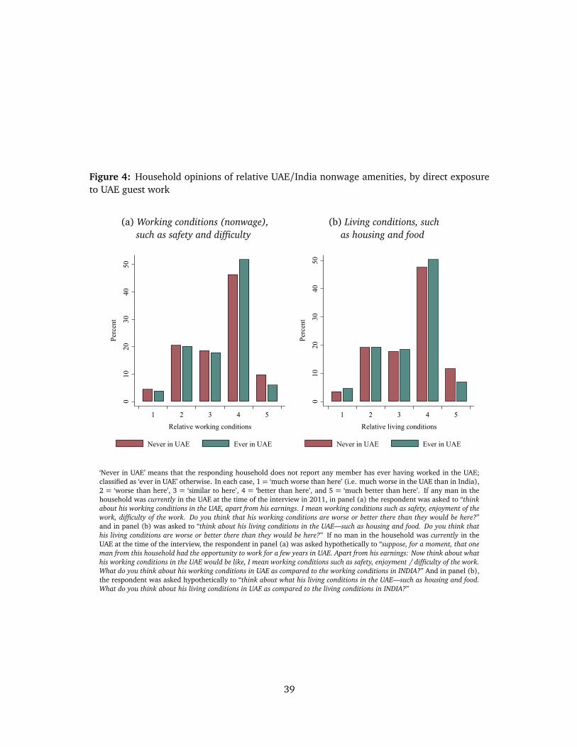
Figure 4: Household opinions of relative UAE/India nonwage amenities, by direct exposureto UAE guest work

(a) Working conditions (nonwage),such as safety and difficulty

010

2030

4050

Perc

ent

1 2 3 4 5

Relative working conditions

Never in UAE Ever in UAE

(b) Living conditions, suchas housing and food

010

2030

4050

Perc

ent

1 2 3 4 5

Relative living conditions

Never in UAE Ever in UAE

‘Never in UAE’ means that the responding household does not report any member has ever having worked in the UAE;classified as ‘ever in UAE’ otherwise. In each case, 1 = ‘much worse than here’ (i.e. much worse in the UAE than in India),2 = ‘worse than here’, 3 = ‘similar to here’, 4 = ‘better than here’, and 5 = ‘much better than here’. If any man in thehousehold was currently in the UAE at the time of the interview in 2011, in panel (a) the respondent was asked to “thinkabout his working conditions in the UAE, apart from his earnings. I mean working conditions such as safety, enjoyment of thework, difficulty of the work. Do you think that his working conditions are worse or better there than they would be here?”and in panel (b) was asked to “think about his living conditions in the UAE—such as housing and food. Do you think thathis living conditions are worse or better there than they would be here?” If no man in the household was currently in theUAE at the time of the interview, the respondent in panel (a) was asked hypothetically to “suppose, for a moment, that oneman from this household had the opportunity to work for a few years in UAE. Apart from his earnings: Now think about whathis working conditions in the UAE would be like, I mean working conditions such as safety, enjoyment / difficulty of the work.What do you think about his working conditions in UAE as compared to the working conditions in INDIA?” And in panel (b),the respondent was asked hypothetically to “think about what his living conditions in the UAE—such as housing and food.What do you think about his living conditions in UAE as compared to the living conditions in INDIA?”

39

Tabl

e9:

Effe

cts

onho

useh

old-

leve

lim

pres

sion

sof

rela

tive

UA

Ew

orki

ngan

dliv

ing

cond

itio

ns

Mea

nβ

OLS

s.e.

βIV

-2SL

Ss.

e.F M

Pβ

IV-D

EV(s

.e.)

N

Trea

tmen

t:An

ym

anfr

omho

useh

old

isno

win

UAE

lnw

age

(act

ualo

rgu

ess)

9.78

0−

0.21

7(0

.030

4)0.

466

(0.4

05)

15.8

80.

226

(0.3

51)

2259

Wor

king

cond

itio

ns(a

ctua

lor

gues

s)3.

310

−0.

0644

(0.0

479)

1.19

7(0

.669)

15.7

20.

842

(0.5

83)

2254

Livi

ngco

ndit

ions

(act

ualo

rgu

ess)

3.36

4−

0.08

16(0

.048

0)0.

263

(0.5

90)

15.4

60.

0900

(0.5

52)

2222

Trea

tmen

t:An

ym

anfr

omho

useh

old

has

ever

been

inU

AEln

wag

e(a

ctua

lor

gues

s)9.

780

−0.

106

(0.0

268)

0.48

0(0

.418)

10.7

80.

298

(0.2

90)

2259

Wor

king

cond

itio

ns(a

ctua

lor

gues

s)3.

310

−0.

0454

(0.0

420)

1.30

2(0

.762)

9.93

10.

909

(0.5

04)

2254

Livi

ngco

ndit

ions

(act

ualo

rgu

ess)

3.36

4−

0.07

04(0

.042

7)0.

282

(0.6

33)

10.1

70.

190

(0.4

68)

2222

Sam

ple

isjo

bap

plic

ants

’hou

seho

lds.

‘Mea

n’is

the

mea

nva

lue

ofth

eou

tcom

ein

the

surv

eysa

mpl

e.O

LSis

ordi

nary

leas

tsq

uare

sw

ith

robu

stst

anda

rder

rors

.IV

-2SL

Sis

two-

stag

ele

ast

squa

res,

wit

h“i

nU

AE”

inst

rum

ente

dby

the

Dub

aiFa

teh

oilp

rice

inde

xon

the

day

ofjo

bap

plic

atio

n,an

dF M

Pis

the

Mon

tiel

-Pflu

eger

(201

3)F

-sta

tist

icte

stin

gth

enu

llof

wea

kin

stru

men

tati

on.

IV-D

EVis

the

dum

my

endo

geno

usva

riab

leIV

mod

el.

All

regr

essi

ons

incl

ude

aco

nsta

ntan

dco

ntro

lsfo

rth

epr

edet

erm

ined

appl

ican

ttr

aits

give

nin

Tabl

e3.

For

the

rati

ngs

ofre

lati

vew

orki

ngan

dliv

ing

cond

itio

ns,1=

‘muc

hw

orse

than

here

’(i.e

.m

uch

wor

sein

the

UA

Eth

anin

Indi

a),2=

‘wor

seth

anhe

re’,

3=

‘sim

ilar

tohe

re’,

4=

‘bet

ter

than

here

’,an

d5=

‘muc

hbe

tter

than

here

’.If

any

man

inth

eho

useh

old

was

curr

ently

inth

eU

AE

atth

eti

me

ofth

ein

terv

iew

in20

11,i

npa

nel(

a)th

ere

spon

dent

was

aske

dto

“thi

nkab

out

his

wor

king

cond

itio

nsin

the

UAE

,apa

rtfr

omhi

sea

rnin

gs.

Imea

nw

orki

ngco

ndit

ions

such

assa

fety

,enj

oym

ento

fthe

wor

k,di

fficu

ltyof

the

wor

k.D

oyo

uth

ink

that

his

wor

king

cond

itio

nsar

ew

orse

orbe

tter

ther

eth

anth

eyw

ould

behe

re?”

and

inpa

nel

(b)

was

aske

dto

“thi

nkab

out

his

livin

gco

ndit

ions

inth

eU

AE—

such

asho

usin

gan

dfo

od.

Do

you

thin

kth

athi

sliv

ing

cond

itio

nsar

ew

orse

orbe

tter

ther

eth

anth

eyw

ould

behe

re?”

Ifno

man

inth

eho

useh

old

was

curr

ently

inth

eU

AE

atth

eti

me

ofth

ein

terv

iew

,the

resp

onde

ntin

pane

l(a)

was

aske

dhy

poth

etic

ally

to“s

uppo

se,f

ora

mom

ent,

that

one

man

from

this

hous

ehol

dha

dth

eop

port

unit

yto

wor

kfo

ra

few

year

sin

UAE

.Apa

rtfr

omhi

sea

rnin

gs:

Now

thin

kab

outw

hath

isw

orki

ngco

ndit

ions

inth

eU

AEw

ould

belik

e,Im

ean

wor

king

cond

itio

nssu

chas

safe

ty,e

njoy

men

t/di

fficu

ltyof

the

wor

k.W

hatd

oyo

uth

ink

abou

this

wor

king

cond

itio

nsin

UAE

asco

mpa

red

toth

ew

orki

ngco

ndit

ions

inIN

DIA

?”A

ndin

pane

l(b)

,the

resp

onde

ntw

asas

ked

hypo

thet

ical

lyto

“thi

nkab

out

wha

thi

sliv

ing

cond

itio

nsin

the

UAE

—su

chas

hous

ing

and

food

.W

hat

doyo

uth

ink

abou

thi

sliv

ing

cond

itio

nsin

UAE

asco

mpa

red

toth

eliv

ing

cond

itio

nsin

IND

IA?”

40

Tabl

e10

:Ef

fect

son

hous

ehol

dbo

rrow

ing

and

debt

Mea

nβ

OLS

s.e.

βIV

-2SL

Ss.

e.F M

Pβ

IV-D

EV(s

.e.)

N

Trea

tmen

t:An

ym

anfr

omho

useh

old

isno

win

UAE

Bor

row

edin

last

3ye

ars?

0.57

80.

0825

(0.0

215)

0.14

8(0

.256)

18.6

40.

107

(0.0

235)

2722

...f

orm

igra

tion

?0.

256

0.18

0(0

.021

1)0.

0791

(0.2

19)

18.6

40.

0883

(0.0

208)

2722

Tota

lbor

row

ed73

532.

516

772.

5(8

891.

8)11

7154

.8(1

4048

1.1)

18.5

218

659.

7(1

2593

.6)

2624

Any

debt

now

?0.

933

−0.

0112

(0.0

122)

−0.

203

(0.1

35)

19.1

20.

0146

(0.0

131)

2569

Am

ount

ofcu

rren

tde

bt39

817.

527

73.9

(525

3.0)

−31

996.

8(1

1377

5.7)

19.1

211

07.0

(101

28.9)

2569

Trea

tmen

t:An

ym

anfr

omho

useh

old

has

ever

been

inU

AEB

orro

wed

inla

st3

year

s?0.

578

0.06

55(0

.019

5)0.

173

(0.3

01)

11.2

50.

108

(0.0

235)

2722

...f

orm

igra

tion

?0.

256

0.14

0(0

.017

6)0.

0925

(0.2

56)

11.2

50.

0930

(0.0

208)

2722

Tota

lbor

row

ed73

532.

522

189.

1(1

0324

.1)

1314

63.9

(158

589.

3)12

.08

1827

8.5

(125

75.2)

2624

Any

debt

now

?0.

933

−0.

0145

(0.0

102)

−0.

228

(0.1

55)

12.5

00.

0150

(0.0

130)

2569

Am

ount

ofcu

rren

tde

bt39

817.

555

11.8

(690

0.2)

−35

811.

8(1

2757

5.2)

12.5

098

4.2

(101

21.5)

2569

Sam

ple

isjo

bap

plic

ants

’hou

seho

lds.

Bor

row

ing

and

debt

mea

sure

din

Indi

anru

pees

.‘M

ean’

isth

em

ean

valu

eof

the

outc

ome

inth

esu

rvey

sam

ple.

OLS

isor

dina

ryle

asts

quar

esw

ith

robu

stst

anda

rder

rors

.IV

-2SL

Sis

two-

stag

ele

ast

squa

res,

wit

h“i

nU

AE”

inst

rum

ente

dby

the

Dub

aiFa

teh

oilp

rice

inde

xon

the

day

ofjo

bap

plic

atio

n,an

dF M

Pis

the

Mon

tiel

-Pflu

eger

(201

3)F

-sta

tist

icte

stin

gth

enu

llof

wea

kin

stru

men

tati

on.

IV-D

EVis

the

dum

my

endo

geno

usva

riab

leIV

mod

el.

All

regr

essi

ons

incl

ude

aco

nsta

ntan

dco

ntro

lsfo

rth

epr

edet

erm

ined

appl

ican

ttr

aits

give

nin

Tabl

e3.

41

Online Appendix“Household effects of temporary low-skill work visas:

Evidence from the India-Gulf corridor”

A1 Descriptive statistics

Table A1 presents descriptive statistics for the variables used in the regressions in the main text.

A2 Global stock of legal low-skill temporary workers

Sources for country totals of legal temporary workers are presented in Appendix Table A2. Data forthe labor force size of Argentina (19.1m), Poland (18.5m), and the 31 other countries with the largestlabor forces in 2013 are from the International Labor Organization, as reported by the World BankWorld Development Indicators (SL.TLF.TOTL.IN, accessed Feb. 1, 2015).

A3 Nationally-representative data

A3.1 India National Sample Survey (NSS) 2008

Education levels are defined according to cases of l4educationgen: “Illiterate” = 1; “Read & Write” =2–6; “Primary” = 7; “Preparatory” = 8; “Secondary” = 10; “Above Secondary” = 11–12; “University”= 13; “Above University” = 14.

‘Relevant’ occupations are defined for the India NSS data, according to India’s National Classificationof Occupations 2004, as: 712 “Building Frame and Related Trades Workers”; 713 “Building Finishersand Related Trades Workers”; 714 “Painters, Building Structure Cleaners and Related Trades Workers”;721 “Metal Moulders, Welders, Sheet Metal Workers, Structural Metal Preparers and Related TradesWorkers”; 724 “Electrical and Electronic Equipment Mechanics and Fitters”; 742 “Wood Treaters, Cab-inet Makers and Related Trades Workers”; 821 “Metal and Mineral Products Machine Operators”; 831“Locomotive Engine Drivers and Related Workers”; 832 “Motor Vehicle Drivers”; 931 “Mining and Con-struction Labourers”; 516 “Protective Services Workers”.

Because the India NSS uses sampling (probability) weights and the UAE LFS uses relative weights,the NSS weights are adjusted to relative weights when the datasets are stacked together. That is, theNSS sampling weights are multiplied by the ratio of sample size to the sum of the sampling weights—converting them to relative weights.

A3.2 UAE Labor Force Survey (LFS) 2008

Education levels are defined according to cases of Q108_C: “Illiterate” = 1; “Read & Write” = 2; “Pri-mary” = 3; “Preparatory” = 4; “Secondary” = 5; “Above Secondary” = 6; “University” = 7; “AboveUniversity” = 8–10. Wage is calculated as total of wage in cash and in kind. The wage reported indirhams is converted to rupees at the exchange rate of |10.99/dirham, which was the average ex-change rate during the period that the NSS data was collected (July 2007–June 2008). Nationals ofcountries other than UAE and India are dropped.

A-1

Appendix Table A1: Descriptive statistics

Variable Mean Std. Dev. Min. Max. N

Individual applicants

In UAE now? 0.297 0.457 0 1 2715In UAE ever? 0.488 0.5 0 1 2715ln wage 8.963 0.935 4.828 12.766 1557Employed? 0.875 0.331 0 1 2715Age 29.015 5.765 20 65 2712Skilled? 0.4 0.49 0 1 2715Semiskilled? 0.487 0.5 0 1 2715Rural? 0.67 0.47 0 1 2715Muslim? 0.302 0.459 0 1 2715

Individual non-applicant adults

Employed? 0.294 0.455 0 1 8552Any wage inc.? 0.232 0.422 0 1 8552ln wage 8.359 1.051 4.423 11.562 1986In UAE now? 0.016 0.126 0 1 8552Overseas now? 0.027 0.162 0 1 8552

Households

Household size (in India) 5.264 2.989 1 34 2723ln income/cap. 7.42 1.128 1.427 11.051 2480Any remittances? 0.344 0.475 0 1 2723ln remittances/cap. 6.965 1.215 2.408 10.714 936ln total expenses/cap. 7.042 0.772 3.954 9.898 2245

. . . food 6.315 0.736 3.624 9.17 2701

. . . quality of life 5.466 1.291 −3.232 8.987 2710

. . . medical 4.486 1.243 0.174 8.74 2526

. . . education 4.294 1.4 −0.875 9.028 1844

. . . durable goods 3.462 1.68 −1.435 8.805 1532Any business profit? 0.088 0.283 0 1 2723Business revenue 359.062 2118.252 0 51666.668 2723Business profit 182.187 1411.569 −5000 45000 2723Own television 0.774 0.418 0 1 2723. . . sewing machine 0.278 0.448 0 1 2723. . . refrigerator 0.418 0.493 0 1 2723. . . motorcycle 0.484 0.5 0 1 2723ln wage (guess or actual) 9.779 0.686 6.397 12.899 2269working conditions (guess or actual) 3.31 1.022 1 5 2263living conditions (guess or actual) 3.364 1.035 1 5 2231

A-2

Appendix Table A2: Lower bound on global stock of legal low-skill temporary workers

Countries Stock Year Includes Source

GCC 13,600,000 2013 ‘Low-skill’ foreign nationals A, pp. 9, 11.

Malaysia 2,100,000 2013 ‘Visit Pass (Temporary Employment)’ B, p. 128.

Korea 547,300 2011 Low-skill work permit holders C, p. 268

Singapore 533,400 2013 ‘Construction’ & ‘Domestic Worker’ D

Russian Federation 400,000 2011 1.2m work-permit holders, 1/3 low-skill C, p. 290

Germany 168,000 2011 Seasonal only C, p. 255

United States 131,792 2013 H-2A and H-2B E

Canada 84,630 2013 Low-skill workers present on Dec. 1 F, p. 4:

Israel 32,000 2012 Agriculture and construction only C, p. 262.

United Kingdom 16,300 2011 Seasonal only C, p. 305

Italy 15,200 2011 Seasonal only C, p. 265

Finland 12,000 2011 Seasonal only C, p. 251

France 8,000 2011 Seasonal only C, p. 252

New Zealand 7,456 2013 Seasonal agricultural workers G

Sweden 3,800 2011 Seasonal only C, p. 299

Norway 2,500 2011 Seasonal only C, p. 283

Spain 2,200 2011 Seasonal only C, p. 297

Australia 2,000 2013 Seasonal agricultural workers H

Total lower bound 17,666,578

‘Stock’ means the number of workers who are on legal low-skill temporary work visas during anyportion of a year, whether those workers begin and end the year at the destination or arrive at and/ordepart from the destination during that year; these numbers are not flows of new migrants. ‘GCC’is Gulf Cooperation Council. Sources: A: IMF, 2013, Labor Market Reforms to Boost Employment andProductivity in the GCC [Population of GCC, and foreign nationals as % of population from Table 1p. 11. Low skill over 80% from Fig. 6 page 9. Thus 0.8 × 0.384 × (1.2 + 3.8 + 3.1 + 1.8 + 29 +5.5)× 106 = 13.64m]. B: Malaysia Ministry of Finance, 2014, Economic Report 2014/2015. C: OECDInternational Migration Outlook 2013. D: Singapore Ministry of Manpower, 2014, “Foreign WorkforceNumbers”, accessed Nov. 6, 2014. E: US State Dept, 2014, Report of the Visa Office 2013. F: ESDC2014, Overhauling the Temporary Foreign Worker Program. G: NZ Ministery of Business, Innovation,and Employment, 2014, RSE Workers Arrival into New Zealand—RSE Financial Year 2012/2013. H:Henry Sherrell 2014, “An update on the Australian Seasonal Worker Program”.

A-3

‘Relevant’ occupations are defined, for the UAE LFS data, as: 7136 “Workers of electrical wiring in build-ings”; 9313 “Building construction workers”; 3113 “Assistant electrical engineer”; 7221 “Blacksmithsand workers hammers and pistons”; 2145 “Mechanical Engineer”; 2142 “Civil Engineer”; 7122 “Con-struction workers with bricks and stones”; 7123 “Workers Pour Concrete”; 8333 “Operators of cranesand equipment to transport materials”; 7242 “Electrical repair and service equipment and electronicequipment”; 3112 “Assistant Civil Engineer”; 2143 “Electrical Engineer”; 7124 “Njaro constructionand fixtures”; 7135 “Plumbers”; 7143 “Workers installing tiles and wooden flooring Mbtaiw”; 7121“Builders traditional materials”; 7212 “Welders and flame-cutting”; 7245 “Workers install and repairelectrical lines and cables”; 1223 “Business managers and production activity in construction”; 9312“Construction workers and maintenance of roads, dams, etc.”; 7144 “Building structure cleaners”;7125 “Other makers of building structures”; 7133 “Workers put insulation”; 9331 “Drivers and vehi-cles driven by hand or towed Softswitch”; 9141 “Building Service Workers”; 7136 “Workers of electricalwiring in buildings”; 9313 “Building construction workers”; 7122 “Construction workers with bricksand stones”; 7123 “Workers Pour Concrete”; 7124 “Njaro construction and fixtures”; 7135 “Plumbers”;7121 “Builders traditional materials”; 7245 “Workers install and repair electrical lines and cables”;1223 “Business managers and production activity in construction”; 9312 “Construction workers andmaintenance of roads, dams, etc.”; 7144 “Building structure cleaners”; 7125 “Other makers of buildingstructures”; 7133 “Workers put insulation”; 3115 “Assistant Mechanical Engineer”; 7239 “Mechani-cal installation and repair of machinery”; 9141 “Building Service Workers”; 9132 “Cleaners in offices,hotels and institutions”; 8322 “Drivers of small cars, pick-ups”.

A4 Nonresponse bias

Figure A5 shows a moving average of the probability that an applicant on each date had obtained a UAElabor card by November 2011 (which requires physical presence in the UAE), in the sampling universe,broken down by survey attempt outcome. Similar patterns of migration in the sampling universe areobserved for the households that were successfully surveyed, the households whose job application didnot provide enough information to locate their residence (‘bad address’), and households that weresuccessfully located but did not yield a completed survey—either because no one could be found at theresidence, the applicant’s family was found at the residence but refused to participate in the survey, orthe applicant’s family had moved away from the residence.

A5 Children

Table A3 shows estimated effects on individual school-age children of the job applicant. The outcomestested are labor-force participation, school attendance, and indicators of performance (awards) andparental involvement in children’s schooling. The low Montiel-Pflueger F -statistic in all regressionssuggests that all IV coefficients in the table are subject to severe bias from weak instrumentation.

A-4

App

endi

xTa

ble

A3:

Effe

cts

onsc

hool

-age

child

ren

ofth

ejo

bap

plic

ant—

unin

form

ativ

edu

eto

wea

kin

stru

men

tati

on

Mea

nβ

OLS

s.e.

βIV

-2SL

Ss.

e.F M

Pβ

IV-D

EV(s

.e.)

N

Trea

tmen

t:Ap

plic

ant

from

hous

ehol

dis

now

inU

AEEm

ploy

ed?

0.01

33−

0.00

175(0

.008

56)

0.04

36(0

.169)

2.29

20.

0007

10(0

.110)

1124

Any

wag

ein

com

e?0.

0124

−0.

0009

03(0

.008

51)

0.09

39(0

.169)

2.29

20.

0254

(0.1

07)

1124

Insc

hool

?0.

904

−0.

0065

8(0

.023

1)−

0.35

7(0

.548)

2.29

2−

0.12

5(0

.293)

1124

...p

riva

tesc

hool

?0.

586

0.15

8(0

.034

7)−

0.41

7(0

.853)

2.52

9−

0.17

9(0

.460)

1017

Day

sm

isse

d1.

956

−0.

156

(0.2

88)−

2.33

5(7

.220)

2.42

0−

0.06

24(3

.856)

1016

Awar

d?0.

166

0.08

43(0

.029

9)0.

278

(0.6

42)

2.52

90.

207

(0.3

53)

1017

Gui

danc

e?0.

540

0.00

608(0

.038

0)−

0.37

1(0

.860)

2.52

9−

0.06

74(0

.462)

1017

Dis

cuss

teac

her?

0.86

80.

167

(0.1

42)−

2.01

1(3

.653)

2.94

8−

0.26

7(2

.876)

930

Trea

tmen

t:Ap

plic

ant

from

hous

ehol

dha

sev

erbe

enin

UAE

Empl

oyed

?0.

0133

−0.

0022

2(0

.006

70)

0.05

39(0

.214)

0.92

30.

0181

(0.0

955)

1124

Any

wag

ein

com

e?0.

0124

−0.

0007

78(0

.006

55)

0.11

6(0

.230)

0.92

30.

0434

(0.0

934)

1124

Insc

hool

?0.

904

0.01

94(0

.017

8)−

0.44

2(0

.781)

0.92

3−

0.16

2(0

.260)

1124

...p

riva

tesc

hool

?0.

586

0.04

53(0

.031

0)−

0.59

6(1

.342)

0.74

0−

0.20

4(0

.436)

1017

Day

sm

isse

d1.

956

−0.

0120

(0.2

40)−

3.46

8(1

1.51)

0.65

5−

1.19

9(3

.718)

1016

Awar

d?0.

166

0.01

15(0

.024

6)0.

397

(0.9

87)

0.74

00.

139

(0.3

37)

1017

Gui

danc

e?0.

540

0.08

41(0

.032

1)−

0.52

9(1

.369)

0.74

0−

0.14

1(0

.445)

1017

Dis

cuss

teac

her?

0.86

80.

526

(0.2

28)−

3.60

7(7

.984)

0.56

6−

1.07

7(2

.954)

930

Sam

ple

issc

hool

-age

child

ren

ofth

ejo

bap

plic

antw

hen

the

job

appl

ican

tis

the

head

ofth

eho

useh

old.

‘Day

sm

isse

d’is

the

answ

erto

the

ques

tion

,“In

the

last

30da

ys,h

owm

any

days

has

(NA

ME)

mis

sed

scho

olw

hen

itw

asin

sess

ion?

”.‘A

war

d’is

1if

the

answ

eris

“yes

”to

“In

the

last

one

mon

th,d

id(N

AM

E)ge

tan

awar

dor

priz

ein

the

scho

ol?”

and

zero

othe

rwis

e.‘G

uida

nce’

is1

ifth

ean

swer

is“y

es”

to“D

oes

anyo

nein

the

hous

ehol

dhe

lp(N

AM

E)in

stud

ies/

teac

hing/p

rovi

ding

guid

ance

?”an

dze

root

herw

ise.

‘Dis

cuss

teac

her’

is1

ifth

ean

swer

is“y

es”

to“D

urin

gth

ela

ston

eye

ar,h

owm

any

tim

esdi

dso

meo

nefr

omth

efa

mily

disc

uss

(NA

ME)

’ssc

hool

wor

kw

ith

the

teac

her?

”an

dze

root

herw

ise.

‘Mea

n’is

the

mea

nva

lue

ofth

eou

tcom

ein

the

surv

eysa

mpl

e.O

LSis

ordi

nary

leas

tsq

uare

sw

ith

robu

stst

anda

rder

rors

.IV

-2SL

Sis

two-

stag

ele

ast

squa

res,

wit

h“i

nU

AE”

inst

rum

ente

dby

the

Dub

aiFa

teh

oilp

rice

inde

xon

the

day

ofjo

bap

plic

atio

n,an

dF M

Pis

the

Mon

tiel

-Pflu

eger

(201

3)F

-sta

tist

icte

stin

gth

enu

llof

wea

kin

stru

men

tati

on.

IV-D

EVis

the

dum

my

endo

geno

usva

riab

leIV

mod

el.

All

regr

essi

ons

incl

ude

aco

nsta

ntan

dco

ntro

lsfo

rth

epr

edet

erm

ined

appl

ican

ttr

aits

give

nin

Tabl

e3.

Wag

esdo

not

incl

ude

earn

ings

from

hom

e-ba

sed

fam

ilyfa

rm/b

usin

ess.

A-5

Figure A5: Sampling universe: UAE administrative records on probability of applicant arrival,by survey attempt outcome

0.2

0.4

0.6

0.8

1.0

Pr[A

pplic

ant o

btai

ned

UA

E la

bor c

ard]

April2008 July2008 October2008 January2009 April2009Application date

Survey completedBad addressMoved away, absent, or refused

Shaded bands show 95% confidence intervals on local regression, Epanechnikov kernel, bandwidth 15 days, degree 0.

A-6