Embed Size (px)
Citation preview

Measuring the possible impacts of MAFTA
Prepared for the Department of Foreign Affairs and Trade
Centre for International Economics Canberra & Sydney
February 2005

The Centre for International Economics is a private economic research agency that provides professional, independent and timely analysis of international and domestic events and policies.
The CIE’s professional staff arrange, undertake and publish commissioned economic research and analysis for industry, corporations, governments, international agencies and individuals. Its focus is on international events and policies that affect us all.
The CIE is fully self-supporting and is funded by its commissioned studies, economic consultations provided and sales of publications.
The CIE is based in Canberra and has an office in Sydney.
© Centre for International Economics 2005
This work is copyright. Persons wishing to reproduce this material should contact the Centre for International Economics at one of the following addresses.
CANBERRA
Centre for International Economics Ian Potter House, Cnr Marcus Clarke Street & Edinburgh Avenue Canberra ACT
GPO Box 2203 Canberra ACT Australia 2601
Telephone +61 2 6248 6699 Facsimile +61 2 6247 7484 Email [email protected] Website www.TheCIE.com.au
SYDNEY
Centre for International Economics Level 8, 50 Margaret Street Sydney NSW
GPO Box 397 Sydney NSW Australia 2001
Telephone +61 2 9262 6655 Facsimile +61 2 9262 6651 Email [email protected] Website www.TheCIE.com.au

iii
Contents
Summary vi
1 Introduction 1
2 Macroeconomic effects of MAFTA 3 What drives the results? 3 Implications of MAFTA for Australia 4 Implications of MAFTA for Malaysia 9 Impact of MAFTA implementation scenarios 12
3 Sectoral effects of the MAFTA 15 Welfare implications of MAFTA 16 The MAFTA and its impact on Australia–Malaysia trade 18 MAFTA and its impact on Australian sectors 21 MAFTA and its impact on Malaysian sectors 28 Impact on Australian State and Territories 36 Sensitivity analysis 37
A Barriers to bilateral trade 40
B Baseline assumptions 62 Trade liberalisation under the FTA 64
C Dynamic productivity 66
D Economic models used to analyse the trade liberalisation 74
References 86
M E A S U R I N G T H E P O S S I B L E I M P A C T S O F M A F T A

iv
C O N T E N T S
Boxes, charts and tables 1 Change in Australia’s real GDP by cause viii 2 Changes in Australia’s welfare by cause viii 3 Welfare and production gains for Australia from the FTA ix 4 Welfare and production gains for Malaysia from the FTA ix 2.1 Macro-economic effects of MAFTA for Australia 5 2.2 Australia’s consumption and GDP gains from the FTA 6 2.3 Sources of Australia’s gain 7 2.4 Changes in employment and wages in Australia 8 2.5 Macroeconomic effects of MAFTA for Malaysia 10 2.6 Malaysia’s real GDP and consumption gains from the FTA 11 2.7 Sources of Malaysia’s gain from FTA 12 2.8 Australia’s GDP under different implementation scenarios 13 2.9 Australia’s welfare under different implementation
scenarios 13 2.10 Present value of real GDP and consumption under different
phase-in scenarios 14 3.1 Welfare effects of MAFTA 16 3.2 Portion of total increase in bilateral exports by sector 19 3.3 Change in Australian exports to Malaysia by sector 19 3.4 Change in service exports from Australia to Malaysia 21 3.5 Impact of the MAFTA on Australia sectors 22 3.6 Impact of the MAFTA on Malaysian sectors 30 3.7 Change in Gross State Product and employment 36 3.8 Range of variation of welfare for Australia and Malaysia 39 3.9 Range of variation of welfare for Australia and Malaysia
under various ranges of parameter/model input variation 39 A.1 Effective tariff barriers to bilateral merchandise trade 43 A.2 Effects of reducing service barriers in Malaysia 45 A.3 Captured market share of the competitive set 47 A.4 Impacts on public administration, defence, education and
health 51 A.5 Service barriers and post MAFTA impacts for Malaysian
construction 52 A.6 Service barriers and post MAFTA impacts for the finance
industry 54
M E A S U R I N G T H E P O S S I B L E I M P A C T S O F M A F T A

C O N T E N T S
v
A.7 Service barriers and post MAFTA impacts for the insurance industry 56
A.8 Restrictiveness indices for Malaysia selected business services 58
A.9 Service barriers and post MAFTA impacts for business services nec 59
C.1 Selected empirical studies finding dynamic gains from reduced trade protection 70
C.2 Dynamic productivity gains 71 C.3 Comparison of contribution of dynamic productivity to
welfare gains 72 D.1 Economy and industry coverage of APG–Cubed 75 D.2 The effect of changing market rates on results 79 D.3 Mapping between databases — GTAP regions 85
M E A S U R I N G T H E P O S S I B L E I M P A C T S O F M A F T A

vi
Summary
AUSTRALIA AND MALAYSIA are considering entering into a bilateral free trade agreement (MAFTA). The possible economic implications of MAFTA have been assessed using economic models of the global economy. Key findings of the economic analysis are presented below.
MAFTA will lift economic growth and welfare in both Australia and Malaysia.
By 2017 the increase in Australia’s real gross domestic product (GDP) is estimated to peak at approximately 0.03 per cent above what it might otherwise have been (the baseline).
– Welfare, as measured by the change in real consumption, is estimated to peak at around 0.04 per cent above baseline in 2016. Real consumption measures the aggregate quantity of goods and services households can consume given their current and future income flows. The higher real consumption is, the more house-holds consume and hence the greater their welfare.
The increase in Malaysia’s GDP is estimated to peak at 0.20 per cent above baseline, while welfare (real consumption) peaks at 0.34 percent above baseline.
Total gains in welfare for both Australia and Malaysia are maximised if MAFTA is implemented immediately rather than over a 5 or 10 year phase in period.
These findings are premised on:
– the free trade agreement (FTA) being implemented in 2007; and
– the FTA comprising the complete removal of tariffs on bilateral trade, liberalisation of service trade, and dynamic productivity gains associated with the trade liberalisation carried out under the FTA.
The possible economic impacts of the FTA have been quantified using two economy wide frameworks — one to capture the macroeconomic outcomes and time path of effects (the APG–Cubed model), and one to
M E A S U R I N G T H E P O S S I B L E I M P A C T S O F M A F T A

S U M M A R Y
vii
capture a ‘snapshot’ of the changes at a disaggregated sectoral and regional level (the GTAP model).
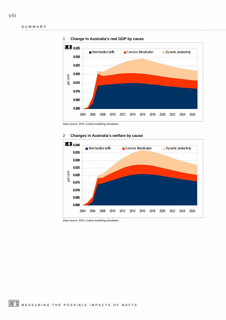
The FTA will have implications over time. As trade liberalisation is generally seen as being a positive step for an economy, additional investment will occur. However, extra investment takes time to put in place. Also, due to differences in agents’ borrowing and lending behaviour and the need to service loans, there is no one annual number that fully reflects the implications of the FTA. The time path of changes in real GDP and welfare (represented by real consumption) for Australia are given below (see charts 1 and 2).
As can be seen from charts 1 and 2, the quantum of changes in real GDP and welfare vary over time. A common way to represent a changing stream of benefits over time is the discounted present value of those benefits. The present value of the net change for Australia’s real GDP is $1.9 billion, while the change in welfare is $1.4 billion, as shown in chart 3. The present value of the net change for Malaysia’s real GDP is RM18.3 billion, while the change in welfare is RM18.2 billion, as shown in chart 4
– The static gains (comprising the results of the removal of merchandise tariffs, and services liberalisation) account for around 76 per cent of the total real GDP and 77 per cent of welfare gains estimated to arise for Australia.
– The static gains account for 96 per cent of Malaysia’s present value gain in real GDP and 95 per cent for welfare.
– With the improved access to the Malaysian market and the greater domestic efficiency that trade liberalisation brings, there is a rise in real investment in Australia that peaks at 0.07 per cent above baseline in 2010. Some of this additional investment is funded by extra capital inflow, which sees a deterioration of the current account by 0.05 per cent of GDP below baseline in 2015.
M E A S U R I N G T H E P O S S I B L E I M P A C T S O F M A F T A
viii
S U M M A R Y
1 Change in Australia’s real GDP by cause
0.000
0.005
0.010
0.015
0.020
0.025
0.030
0.035
2004 2006 2008 2010 2012 2014 2016 2018 2020 2022 2024 2026
per c
ent…
.
Merchandise tariffs Serv ices liberalisation Dynamic productiv ity
Data source: APG–Cubed modelling simulation.
2 Changes in Australia’s welfare by cause
0.000
0.005
0.010
0.015
0.020
0.025
0.030
0.035
0.040
2004 2006 2008 2010 2012 2014 2016 2018 2020 2022 2024 2026
per c
ent…
.
Merchandise tariffs Serv ices liberalisation Dynamic productiv ity
Data source: APG–Cubed modelling simulation.
M E A S U R I N G T H E P O S S I B L E I M P A C T S O F M A F T A

S U M M A R Y
ix
3 Welfare and production gains for Australia from the FTA NPV 2005a
1.93
1.38
0.0
0.5
1.0
1.5
2.0
2.5
Real GDP Real Consumption
A$ b
illion
a Over 2005 to 2027 discounted at a 5 per cent real interest rate. Data source: APG-Cubed modelling simulation
4 Welfare and production gains for Malaysia from the FTA NPV 2005a
18.31 18.18
0
5
10
15
20
25
Real GDP Real Consumption
RM bi
llion
a Over 2005 to 2027 discounted at a 5 per cent real interest rate. Data source: APG-Cubed modelling simulation
Due to the capital inflow there is a small appreciation of the Australia currency. The Australia dollar is stronger against the US dollar in real terms by 0.03 percentage points in 2011.
The growth in the Australia economy has positive implications for workers. The benefits to workers comprise a mix of extra employment and real wage growth that changes over time. With real wages that lag developments in the labour market, there is initially a rising trend in employment, peaking at an increase in employment of 0.02 per cent by 2007. As wages adjust over time, employment falls back to the baseline
M E A S U R I N G T H E P O S S I B L E I M P A C T S O F M A F T A

x
S U M M A R Y
‘natural rate of full employment’, by which time the gains are received via an increase in real wages of 0.03 per cent above baseline in 2027.
As is to be expected, trade liberalisation carried out under the FTA has a substantial impact on bilateral trade flows. Australia exports to Malaysia are estimated to increase by 5.5 per cent. Increases in merchandise exports account for 54 per cent of this increase, with increased services exports accounting for the remaining 46 per cent. Malaysia’s exports to Australia are estimated to increase by 6.3 per cent which is primarily due to an increase in merchandise exports. For modelling purposes, services trade liberalisation by Australia was assumed to not occur under MAFTA.
M E A S U R I N G T H E P O S S I B L E I M P A C T S O F M A F T A

1
1 Introduction
AT THE AUSTRALIA-MALAYSIA Joint Trade Committee Meeting on 26 July 2004, Australia’s Trade Minister Mr Mark Vaile and his Malaysian counterpart, Minister for International Trade and Industry, Rafidah Aziz, agreed that the two countries would conduct parallel scoping studies of a free trade agreement between Australia and Malaysia.
As part of this study the Australian Department of Foreign Affairs and Trade (DFAT) employed the CIE to undertake a detailed modelling exercise to measure the likely impacts to the Australian and Malaysian economies of a WTO consistent free trade agreement between Australia and Malaysia (MAFTA).
To develop a comprehensive analysis, two economic frameworks (global general equilibrium models) have been used to quantify the economic impacts of MAFTA. These include the:
APG–Cubed model; and
Global Trade Analysis Project (GTAP) model.
The APG–Cubed is a dynamic model that allows observation of the effects of the Agreement over time. The dynamic nature of the model is a critical feature as trade liberalisation under MAFTA may involve the phasing out of barriers to merchandise and services trade over time. The model also allows economic agents to have expectations and act in response to announced policy decisions and considers both the real and financial sectors, including international investment links and/or flows between countries. It also allows agents to maximise welfare over time as agents can borrow and/or lend money.
In comparison, the GTAP model is a comparative–static (that is, does not incorporate time) model, but it does incorporate considerable commodity and regional detail. The high level of detail makes GTAP well placed to examine the implications of MAFTA for specific sectors of the economy.
The principal outputs of this study are the estimates of the impacts upon the Australian and Malaysian economies as a result of preferential
M E A S U R I N G T H E P O S S I B L E I M P A C T S O F M A F T A

2
1 I N T R O D U C T I O N
reductions in barriers on merchandise and services trade. The modelling assumes implementation of a comprehensive agreement, with no carve-outs for sensitive sectors. Reductions in trade barriers have been modelled through the removal of ad valorem and specific tariffs on merchandise trade and reductions in barriers to commercial presence and consumption abroad for services trade. The impact of duty drawback schemes on the effective rate of tariffs for merchandise trade has been included in the modelling. A reduction in the barriers to investment has only been accounted for in the services sector.
In addition, this study accounts for possible dynamic productivity gains – additional productivity gains in the merchandise sectors that can result from a reduction in tariffs, which are not revealed by standard economic models. Due to limited empirical data on the possible dynamic productivity gains for Malaysia and Australia, the study has used conservative estimates with an associated sensitivity analysis around these estimates.
However, while this study has taken into consideration important non-tariff barriers, it has not explicitly set out to model the impacts that may result from a reduction in these types of barriers. Consequently the study does not account for any benefits that may result from encouraging effective national competition regimes or improved customs and standards issues.
Furthermore, the study does not take into account the impact of rules of origin. This is because it is not yet known which type of rules of origin regime Australia and Malaysia will agree upon and for the products to which it will apply.
As with all modelling, results are driven in part by key assumptions on model parameters and estimates of key inputs. To derive these parameters and inputs, the CIE has used the most relevant and up to date information available. Where data have not been readily available, the CIE has used conservative estimates based on anecdotal evidence and consultations with industry groups. To ensure robustness of results, a sensitivity analysis has also been conducted on these model parameters and key inputs.
M E A S U R I N G T H E P O S S I B L E I M P A C T S O F M A F T A

3
2 Macroeconomic effects of MAFTA
THE PROPOSED FREE TRADE AGREEMENT between Australia and Malaysia will have implications for growth, trade and investment flows in both countries. Being a fully dynamic model that integrates goods and financial markets with a sophisticated treatment of assets and financial variables, the APG–Cubed model is well placed to explore the implications of the FTA for the macro-economy. The implications for the macro-economic variables of (real) gross domestic product, welfare, exports and imports, investment, the exchange rate and employment are reported for both countries until year 2027.
The change in GDP is the commonly used measure of the change in economic welfare resulting from trade liberalisation. However, changes in real GDP reflect only changes in the overall level of economic activity and not changes in (net) national income or welfare per se. Given the likely change in income flows, the change in real consumption is used as the primary indicator of the welfare gains because it captures only the income flows accruing to domestic residents (that is, foreigner’s earnings are excluded). The real consumption measures the aggregated quantity of goods and services the households can consume given their current and future income flows. The higher the real consumption is, the more the households enjoy, and thus, the more welfare they gain. Being a dynamic model, APG–Cubed is able to take into account the implications for the time path of welfare since it formally incorporates borrowing and lending behaviour, both locally and internationally, and accounts for the need to service those loans.
What drives the results? The magnitude of the effects reported below is primarily determined by several factors, namely:
the size of barriers to trade imposed by Australia and Malaysia;
the contribution of exports and imports to GDP;
M E A S U R I N G T H E P O S S I B L E I M P A C T S O F M A F T A

4
2 M A C R O E C O N O M I C E F F E C T S O F M A F T A
the extent of bilateral trade between the two countries; and
the extent of dynamic productivity improvement implied by trade liberalisation.
Australia has lower barriers to trade than Malaysia does. This implies that the latter may benefit more from the FTA than the former.
Agents’ behaviour in the APG model includes forward–looking expectations, and this will have some bearing on the results. For example, household’s consumption in one period is determined by the lifetime wealth as well as by the current income at point in time. In the long run, these two behaviours converge. Because of this specification of agents’ behaviour, overshooting and kinks may be observed in some years.
Implications of MAFTA for Australia The macro-economic effects of the FTA on the Australian economy are shown in the series of five figures that follow. The reported results pertain to a scenario of immediate trade liberalisation in 2007. The total impacts are a combination of the following liberalisation measures:
merchandise trade liberalisation in Australia and Malaysia, which in turn consists of:
− complete removal of each country’s tariffs on bilateral merchandise trade in 2007;
services sector liberalisation:
− reduction of Malaysia’s tariff-equivalent barriers on service imports from Australia in 2007 and increased commercial presence by Australian service providers in Malaysia;
− assuming for modelling purposes there is no additional trade liberalisation of Australian service sectors due to their already very open nature; and
dynamic productivity improvement associated with the above trade liberalisation phased in over ten years beginning 2007 (productivity gains are phased in to reflect time taken by producers to respond to increased competition from imports).
Macroeconomic effects
The macro-economic effects of MAFTA are reported in chart 2.1. For Australia, MAFTA brings about a small positive impact. Both output and
M E A S U R I N G T H E P O S S I B L E I M P A C T S O F M A F T A

2 M A C R O E C O N O M I C E F F E C T S O F M A F T A
5
2.1 Macro-economic effects of MAFTA for Australia
Real GDP
0.00
0.01
0.02
0.03
0.04
2004 20062008 2010 2012 20142016 2018 2020 20222024 2026
% d
eviat
ion fr
om b
aseli
ne …
...
Real Consumption
0.00
0.01
0.02
0.03
0.04
2004 20062008 20102012 20142016 2018 20202022 20242026
% d
eviat
ion fr
om b
aseli
ne …
…..
Real imports and exports
-0.10
0.00
0.10
0.20
0.30
0.40
200420062008201020122014201620182020202220242026
% d
eviat
ion fr
om b
aseli
ne …
... Ex ports
Imports
Real investment
0.00
0.02
0.04
0.06
0.08
20042006 200820102012 2014201620182020 202220242026
% d
eviat
ion fr
om b
aseli
ne …
..
Exchange rate (against US$)
0.00
0.01
0.02
0.03
0.04
0.05
20042006 200820102012 2014201620182020 202220242026
% d
eviat
ion fr
om b
aseli
ne …
.. Nominal
Real
Change in current account deficit
0.0
0.2
0.4
0.6
2004 2006 2008 2010 2012 2014 2016 2018 2020 2022 2024 2026
%
Data source: APG–Cubed modelling simulation.
welfare increase above the baseline after the FTA commences. The rise in real GDP peaks a decade out at 0.03 per cent above baseline. Real consumption — the preferred welfare measure — peaks a decade out at almost 0.04 per cent above baseline.
With the improved access to the Malaysian market, there is a lift in exports from Australia amounting to 0.37 per cent above baseline in 2007, with the increase slightly declining to 0.33 per cent two decades out.
M E A S U R I N G T H E P O S S I B L E I M P A C T S O F M A F T A

6
2 M A C R O E C O N O M I C E F F E C T S O F M A F T A
With the rise in economic activity and lower barriers to Malaysia imports, there is an increase in imports as well. However, the magnitude of the import rise is smaller than that of export rise (in percentage terms). Australia’s total imports rise by about 0.31 per cent above baseline after the commencement of MAFTA. As imports are larger than exports in absolute terms, the rise in exports is not sufficient to fully offset the rise in imports in absolute terms. With the increase in imports exceeding the increase in exports, the current account deficit deteriorates.
The deterioration in the current account deficit in turn implies greater capital inflow than would have otherwise been the case. Domestic invest-ment rises to a peak of 0.07 per cent higher above the baseline around 2010. The higher demand for Australian currency leads to slight real appreciation of the Australian dollar.
Welfare and production gains
The additional welfare (real consumption) and production (real GDP) gains under MAFTA are reported in chart 2.2. Results are presented in net present value (NPV) terms, which allows a current value to be placed on gains that may not be experienced until some time in the future. Australia gains A$1.93 billion in real GDP and A$1.38 billion in real consumption.
2.2 Australia’s consumption and GDP gains from the FTA NPV 2005a
1.93
1.38
0.0
0.5
1.0
1.5
2.0
2.5
Real GDP Real Consumption
A$ b
illion
a Over 2005 to 2027 discounted at a 5 per cent real interest rate. Data source: APG–Cubed modelling simulation.
M E A S U R I N G T H E P O S S I B L E I M P A C T S O F M A F T A

2 M A C R O E C O N O M I C E F F E C T S O F M A F T A
7
Sources of benefits
The sources of gains to Australia are examined in two ways. First, we investigate the impact of each country’s own trade liberalisation on the gains. Second, the impacts are decomposed into gains from merchandise trade liberalisation, services trade liberalisation and dynamic productivity improvement associated with the trade liberalisation. Chart 2.3 reports the composition of the net present value of Australia’s gains in real GDP and real consumption.
2.3 Sources of Australia’s gain NPV 2005a
0.0
0.5
1.0
1.5
2.0
2.5
Real GDP Real Consumption
A$ b
illion
Malaysian liberalisationAustralian liberalisation
0.0
0.5
1.0
1.5
2.0
2.5
Real GDP Real Consumption
A$ b
illion
Dynamic productiv ityServ ice liberalisationMerchandise liberalisation
a Over 2005 to 2027 discounted at a 5 per cent real interest rate. Data source: APG-Cubed modelling simulation
As shown in chart 2.3, most of the Australia’s gains in real GDP come from Malaysia’s trade liberalisation against Australia imports. In net present value terms, about 51 per cent of increased real GDP and 77 per cent of increased real consumption are due to Malaysia’s trade liberalisation and associated dynamic productivity improvement.
It is also evident from chart 2.3 that most of the gains are due to merchandise trade liberalisation. In terms of net present value, about 55 per cent of gains in real GDP and 60 per cent of gains in real consumption can be attributed to merchandise trade liberalisation. Service liberalisation and dynamic productivity gains have smaller impacts, each accounting for around 20 per cent of the total gains.
M E A S U R I N G T H E P O S S I B L E I M P A C T S O F M A F T A

8
2 M A C R O E C O N O M I C E F F E C T S O F M A F T A
Employment
Although APG–Cubed assumes fixed labour supply and full employment determined by the population growth rate in the long run, in the short run employment deviates from the full employment equilibrium level because wages adjust slowly in response to changing demand for labour. After MAFTA commences, increases in production bring about higher demand for labour. Although real wages increase initially, it is not sufficient to depress the higher labour demand, resulting in increased employment. Over time, wages adjust (increase) to ensure that employment falls back to its baseline level. The long term gain to employment is reflected in higher real wages.
MAFTA is forecast to have a positive, but small, impact on employment in Australia. As shown in chart 2.4, after a downward adjustment before the proposed liberalisation, employment in Australia increases and peaks at 0.02 per cent higher than the baseline level in 2007 and then gradually returns back to the baseline level — the natural rate of unemployment.
2.4 Changes in employment and wages in Australia
-0.01
0.00
0.01
0.02
0.03
2004 2006 2008 2010 2012 2014 2016 2018 2020 2022 2024 2026
% d
eviat
ion fr
om b
aseli
ne
Employment
Real wage rate
Data source: APG–Cubed modelling simulation.
Chart 2.4 also shows that the real wage rate, which is the difference between the nominal wage rate and inflation, increases over time and reaches 0.03 per cent higher than the baseline level around 2020.
Employment is forecast to drop below the baseline level from 2023. Although this deviation is very small, being less than one hundredth of a percentage point, it may cause concerns to some groups. Three points should be emphasised in interpreting this result. First, it does not mean the
M E A S U R I N G T H E P O S S I B L E I M P A C T S O F M A F T A

2 M A C R O E C O N O M I C E F F E C T S O F M A F T A
9
employment level is lower than the current level, it is just slightly below the level that it might have otherwise been in more than twenty years, with employment still being projected to rise over time. Second, even though employment is slightly lower than the baseline, the real wage rate is still 0.03 per cent higher than the baseline. Third, the drop below baseline is a temporary deviation from the long run equilibrium. If chart 2.4 was extended beyond 2027 it can be seen that employment picks up and gradually returns to the baseline level in the longer period, with there being a permanent increase in the real wage rate by 0.03 per cent.
Implications of MAFTA for Malaysia The focus of this study is on the impact of the proposed FTA on the Australian economy. However, summary results about the effects of the FTA on Malaysia are provided for comprehensiveness and comparability.
As shown in chart 2.5, MAFTA will have a positive impact on Malaysia, and with the impacts being larger in magnitude than was the case for Australia. The principal reason for this is that Malaysia has a higher degree of protection, and hence a more distorted economy, than Australia.
Real GDP and real consumption in Malaysia will be 0.20 and 0.34 per cent higher than the baseline level ten years out. Real consumption in Malaysia is expected to substantially increase beginning year 2006. This is in contrast to Australia, where real consumption is forecast to substantially increase in 2004. Real consumption in Australia increases prior to MAFTA being implemented due to forward looking expectations exhibited by economic agents. With the (assumed) announcement that MAFTA will commence in 2007, economic agents expect that future income will be higher as a result of the FTA. As economic agents can borrow and lend money in the APG–Cubed model, the expectation of higher future income as a result of MAFTA sees agents borrowing money and bringing forward future consumption, which acts as a stimulus to economic activity (GDP and output) and raises welfare (consumption).
In Malaysia, increases in real consumption are delayed (relative to that experienced by Australia) due to households allocating a greater share of disposable income to savings rather than consumption. The decision to save more and consume less is made in response to a small rise in the real interest rate (not shown). Interest rates rise due to the Malaysian economy expanding and needing greater capital. Higher interest rates promote greater savings, and this in turn allows (in part) investment to increase. As the capital requirements are met the interest rate declines, and households
M E A S U R I N G T H E P O S S I B L E I M P A C T S O F M A F T A

10
2 M A C R O E C O N O M I C E F F E C T S O F M A F T A
2.5 Macroeconomic effects of MAFTA for Malaysia
Real GDP
0.00
0.05
0.10
0.15
0.20
0.25
2004 20062008 2010 2012 20142016 2018 2020 20222024 2026
% d
eviat
ion fr
om b
aseli
ne
Real Consumption
0.00
0.10
0.20
0.30
0.40
2004 2006 20082010 2012 2014 2016 2018 20202022 2024 2026
% d
eviat
ion fr
om b
aseli
ne
Exchange rate (against US$)
-0.10
0.00
0.10
0.20
0.30
0.40
200420062008201020122014201620182020202220242026
% d
eviat
ion fr
om b
aseli
ne
Imports
Ex ports
Exchange rate (against US$)
-0.01
0.00
0.01
0.02
0.03
200420062008201020122014201620182020202220242026
% d
eviat
ion fr
om b
aseli
ne
Real
Nominal
Change in current account surplus
-1.50
-1.00
-0.50
0.00
0.50
1.00
20042006 20082010 201220142016 20182020 202220242026
% d
eviat
ion fr
om b
aseli
ne
Real investment
0.00
0.10
0.20
0.30
0.40
2004 2006 2008 2010 2012 20142016 2018 2020 2022 2024 2026
% d
eviat
ion fr
om b
aseli
ne
Data source: APG–Cubed modelling simulation.
switch from savings to consuming, hence real consumption increases from 2006 onwards.
The change in exports and imports is of a similar magnitude, although the increase in exports is marginally higher than the change in imports in the early years of MAFTA. The similar change in exports and imports lead to a small improvement in the current account. Immediately following implementation of MAFTA the current account surplus increases by 0.77 per cent, then dampens to 0.07 per cent twenty years out. To maintain a balance in the Balance of Payments (a long run requirement), there will be capital outflows from Malaysia initially and a real depreciation of the Malaysian Ringgit to offset/counteract the increase in the current account
M E A S U R I N G T H E P O S S I B L E I M P A C T S O F M A F T A

2 M A C R O E C O N O M I C E F F E C T S O F M A F T A
11
surplus. As the current account surplus dampens over time, the Ringgit appreciates gradually in real terms. However, because of the increase in output, input prices are expected to increase for most of the sectors, thereby driving up the aggregate domestic price and reducing the nominal exchange rate. Hence there may be pressure on Malaysia to adjust the rate at which the Ringgit is pegged to the USD.
MAFTA sees one set of distortions being removed from the Malaysian economy. As such, economic efficiency rises and hence capital earns a higher return. This leads to greater investment in the domestic economy, with investment peaking at 0.27 per cent above baseline five years after the commencement of MAFTA.
As shown in chart 2.6, the net present value of Malaysia’s gains in real GDP and real consumption over 2005 to 2027 are, respectively, RM18.31 billion and RM18.18 billion.
Different to the Australian case, Malaysia will benefit the most from its own trade liberalisation. Over 72 and 71 per cent of Malaysia’s gains in real GDP and real consumption, respectively, are due to its own trade liberalisation and associated dynamic productivity gains. This is because Malaysia has a more distorted trade regime than Australia. Service trade liberalisation is the primary source of gains to Malaysia, accounting for 56.8 per cent of gains in real GDP and 64.4 per cent of gains in real consumption. This is closely followed by merchandise trade liberalisation,
2.6 Malaysia’s real GDP and consumption gains from the FTA NPV 2005a
18.31 18.18
0
5
10
15
20
25
Real GDP Real Consumption
RM b
illion
a Over 2005 to 2027 discounted at a 5 per cent real interest rate. Data source: APG-Cubed modelling simulation.
M E A S U R I N G T H E P O S S I B L E I M P A C T S O F M A F T A

12
2 M A C R O E C O N O M I C E F F E C T S O F M A F T A
attributing to 38.8 per cent of gains in GDP and 30.3 per cent gains in real consumption (see chart 2.7).
2.7 Sources of Malaysia’s gain from FTA NPV 2005a
0
5
10
15
20
25
Real GDP Real Consumption
RM b
illion
Malaysia unilateral liberalisationAustralia unilateral liberalisation
0
5
10
15
20
25
Real GDP Real ConsumptionRM
billi
on
Dynamic productivityService liberalisationMerchandise liberalisation
a Over 2005 to 2027 discounted at a 5 per cent real interest rate. Data source: APG-Cubed modelling simulation.
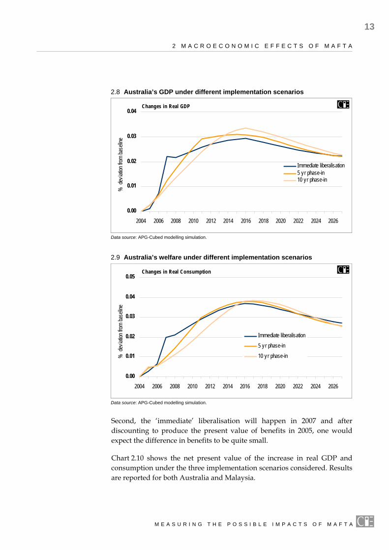
Impact of MAFTA implementation scenarios The above results report the effect for Australia and Malaysia from the immediate removal of bilateral trade barriers under MAFTA (with implementation in year 2007). We now consider what happens when Australia and Malaysia phase in the removal of trade barriers over time. Two scenarios are considered — 5 year and 10 year phase-ins (commencing in 2007). In each scenario, the same percentage point reduction in trade barriers occurs every year after 2007 until the full liberalisation is achieved in the specified time period.
Charts 2.8 and 2.9 show the paths of Australia’s real GDP and real consumption of immediate liberalisation, five year phase in and ten year phase in. It can be seen from these charts that immediate liberalisation leads to a larger and earlier increase in welfare (as measured by real con-sumption). Those results are as expected — removing trade barriers earlier results in a greater gain net of adjustment costs (which are incorporated and allowed for in this model). The results for Australia show that the greatest gain in welfare (real consumption) is when trade barriers are removed immediately. But the difference among the three implementation scenarios considered is not overly large due to two reasons. First, Australia already has very low levels of protection, so the gain resulting from immediate liberalisation is not large after netting of adjustment costs.
M E A S U R I N G T H E P O S S I B L E I M P A C T S O F M A F T A
2 M A C R O E C O N O M I C E F F E C T S O F M A F T A
13
2.8 Australia’s GDP under different implementation scenarios
0.00
0.01
0.02
0.03
0.04
2004 2006 2008 2010 2012 2014 2016 2018 2020 2022 2024 2026
% de
viatio
n from
base
line .
..
Immediate liberalisation5 yr phase-in10 yr phase-in
Changes in Real GDP
Data source: APG-Cubed modelling simulation.
2.9 Australia’s welfare under different implementation scenarios
0.00
0.01
0.02
0.03
0.04
0.05
2004 2006 2008 2010 2012 2014 2016 2018 2020 2022 2024 2026
% de
viatio
n from
base
line …
.
Immediate liberalisation
5 yr phase-in
10 yr phase-in
Changes in Real Consumption
Data source: APG-Cubed modelling simulation.
Second, the ‘immediate’ liberalisation will happen in 2007 and after discounting to produce the present value of benefits in 2005, one would expect the difference in benefits to be quite small.
Chart 2.10 shows the net present value of the increase in real GDP and consumption under the three implementation scenarios considered. Results are reported for both Australia and Malaysia.
M E A S U R I N G T H E P O S S I B L E I M P A C T S O F M A F T A

14
2 M A C R O E C O N O M I C E F F E C T S O F M A F T A
As can be seen, the difference among the alternative implementation scenarios considered is larger for Malaysia. This is because Malaysia’s trade protection is relatively higher than Australia’s, and therefore the gains from trade liberalisation are larger after netting of adjustment costs. Delaying such large potential gains, as the slower phase in scenarios do, translates into a substantial reduction in gains when results are expressed in present value terms.
2.10 Present value of real GDP and consumption under different phase-in scenarios 2005a
Australia
0.0
0.5
1.0
1.5
2.0
2.5
Real GDP Real Consumption
immediate liberalisationphase-out in 5 yearsphase-out in 10 years
Pres
ent v
alue
(A$
billio
n)…...
Malaysia
0
5
10
15
20
25
Real GDP Real Consumption
Pres
ent v
alue
(RM
billi
on)…
.
immediate liberalisationphase-out in 5 yearsphase-out in 10 years
a Over 2005 to 2027 discounted at a 5 per cent real interest rate. Data source: APG–Cubed modelling simulation.
M E A S U R I N G T H E P O S S I B L E I M P A C T S O F M A F T A
15
3 Sectoral effects of the MAFTA
THE MAFTA IS EXPECTED to have varying impacts at the sectoral level due to the disparity in individual sectors’ protection and the resultant reduction in barriers. With its considerable commodity (and regional) detail, the GTAP framework is well suited to examining the implications for the various sectors of the economy of the bilateral trade liberalisation carried out under the MAFTA.
For each identified sector of the economy, GTAP results are provided for (changes to) production and employment, export and import volumes, and prices received by local producers. GTAP uses a slightly different measure of welfare than that reported in the APG–Cubed modelling. The welfare measure reported by GTAP is ‘equivalent variation’. Equivalent variation represents the additional income that would need to be given to the community to make consumers as well off as they would have been under MAFTA.
It is important to appreciate that the APG–Cubed and GTAP welfare results are not comparable. APG–Cubed measures welfare by the change in real consumption, whereas GTAP measures the impact on welfare via changes in equivalent variation, and these are different measures. Furthermore, the models themselves are very different. APG–Cubed is well placed to track the macro-economic impacts of MAFTA over time as it is a fully dynamic macro-economic model that incorporates the real and financial sectors. In contrast, GTAP is a comparative static model — it provides a ‘snapshot’ of what the economy will look like in the long run, but no detail on how the economy gets to that long run position, nor can it properly account for the cumulative effects of MAFTA overtime. GTAP does, however, identify a multitude of different sectors of the economy, making it better placed to investigate the sectoral impacts of MAFTA. The upshot being, the GTAP and APG–Cubed results should not be compared.
Finally, although the GTAP framework provides significant sectoral detail and can provide important insights about the effects of inter-industry linkages, the results should, as with all economic models, be regarded with caution. The response of any given sector to trade liberalisation depends on
M E A S U R I N G T H E P O S S I B L E I M P A C T S O F M A F T A

16
3 S E C T O R A L E F F E C T S O F T H E M A F T A
a complex set of factors affecting both demand and supply, which are difficult to capture with precision in any model. The important things economic models indicate is the mechanisms at work and the insights gained.
Welfare implications of MAFTA The GTAP modelling has been conducted so that the individual factors contributing to changes in Australia’s and Malaysia’s welfare can be identified. Table 3.1 shows the expected welfare gains from MAFTA broken down into its component parts – the gains to welfare from tariff liberalisation by both countries, dynamic productivity gains in both countries, and the service trade liberalisation of both countries (for example the table shows that Australia is expected to gain $1.0 million from reducing its own tariff barriers and $42.8 million from Malaysia reducing their tariff barriers as part of the total $186.3 million expected equivalent variation).
In addition to welfare gains, under the GTAP model GDP is also expected to increase by $164.5 million for Australia and RM513.2 million for Malaysia.
3.1 Welfare effects of MAFTA
Equivalent
Variation Tariff liberalisation Dynamic productivity Service trade liberalisation
Australia Malaysia Australia Malaysia Commercial
presence Consumption
abroad
Australia $ milliona 186.3 1.0 42.8 65.9 0.3 34.2 42.1Malaysia RM milliona 719.2 175.4 55.1 -0.9 108.6 381.0 0a Exchange rates of 1USD = AUD1.29 and 1USD = RM3.8 have been used. Source: CIE calculations
Australia
As can be seen, MAFTA has positive welfare effects for Australia irrespective of which sources of economic impact are considered. If merchandise and services trade is liberalised and dynamic productivity gains occur, then Australia’s welfare is estimated to rise by $186.3 million per year as a result of MAFTA. If only merchandise trade liberalisation occurs without any dynamic productivity improvements or services trade liberalisation, then Australia’s welfare is estimated to increase by $43.8 million per year.
M E A S U R I N G T H E P O S S I B L E I M P A C T S O F M A F T A

3 S E C T O R A L E F F E C T S O F T H E M A F T A
17
While merchandise trade liberalisation is an important contributor to the welfare gain, accounting for around 24 per cent of Australia’s total gain, the effect of liberalising Malaysia’s service barriers is also very important. Service barrier liberalisation is estimated to account for around 41 per cent of Australia’s welfare gain. This reflects the expected increase in tourism exports from Australia to Malaysia (and the increase in related expenditure that is associated with a greater number of Malaysian tourists) and the increase in commercial presence.
Dynamic productivity gains, arising through increased price competition from now cheaper imports, have a positive impact on Australia’s welfare. Productivity gains in the Australia merchandise sectors deliver an almost $66 million improvement in welfare. Malaysia’s liberalisation is associated with its sectors experiencing productivity gains primarily in manu-facturing. As such, Malaysia’s dynamic productivity gains lead to price declines in manufacturing exports, and hence lower priced manufacturing imports from Malaysia are received in Australia. This has a welfare improving effect in Australia (as Australian consumers and businesses can now purchase more imports for the same expenditure). Malaysia’s dynamic productivity gains are associated with Australian welfare rising by $0.3 million. Overall, dynamic productivity improvements yield a welfare gain of $66.2 million (or 36 per cent of total gains) to Australia.
Malaysia
MAFTA is estimated to deliver a RM719.2 million gain in Malaysia’s welfare. Merchandise trade liberalisation accounts for approximately 32 per cent of this total, comprising gains from Australia’s liberalisation of its merchandise barriers (RM175.4 million) and cheaper production inputs into Malaysia as a result of Malaysia’s liberalisation of its own merchandise barriers (RM55.1 million).
Service trade liberalisation contributes significantly to Malaysia’s welfare improvement, accounting for approximately RM381 million, or 53 per cent of the total gain. The welfare gain from service trade liberalisation is derived from a reduction in barriers to commercial presence. An increase in foreign competitors reduces the economic rent captured by incumbents and increases productivity within (some) service sectors. In total, the gain in welfare from merchandise trade liberalisation and service liberalisation is approximately RM611.5 million, accounting for 85 per cent of the total gain.
Dynamic productivity gains as a result of merchandise trade liberalisation in Malaysia account for approximately RM108 million, or 15 per cent of the total gain. This gain is smaller (when expressed in a common currency)
M E A S U R I N G T H E P O S S I B L E I M P A C T S O F M A F T A

18
3 S E C T O R A L E F F E C T S O F T H E M A F T A
than the welfare gain experienced by Australia as a result of dynamic productivity. However, Malaysia’s welfare gain from dynamic productivity expressed as a share of GDP is relatively larger at 0.02 per cent than Australia’s at 0.008 per cent. This is because Malaysia has large dynamic productivity gains off a small GDP base, whereas Australia has small dynamic productivity gains off a relatively larger GDP base. Malaysia experiences relatively larger proportional gains due to a larger reduction in merchandise trade barriers for the majority of its industries.
In table 3.1 it can be seen that Australia’s welfare improves as a result of Malaysia’s dynamic productivity gains, whereas Malaysia’s welfare declines as a result of dynamic productivity gains in Australia. This latter result arises due to the incidence of tariffs in Australia and the nature of exports in Malaysia. Australia’s highest tariffs are in the manufacturing sectors, and hence these sectors experience the larger dynamic productivity gains. The productivity gain improves the competitive position of Australian made manufactures in both the domestic market and exports markets. Malaysia exports predominantly manufactured goods, hence Australia’s productivity gains in the manufacturing sectors acts to displace some Malaysian imports from both the Australian market and third country markets, which has a slight negative effect on Malaysian welfare.
As with any quantitative analysis, the results are sensitive to the assumptions underlying the model. Sensitivity analysis of the welfare results presented in table 3.1 are included at the end of this chapter.
The MAFTA and its impact on Australia–Malaysia trade Exports between Australia and Malaysia increase significantly as a result of MAFTA. Australia is forecast to increase its total exports to Malaysia by $198.3 million, or 5.5 per cent while Malaysia increases its total exports to Australia by RM760.4 million, or 6.3 per cent. Chart 3.2 shows the breakdown of the increase in exports for both Australia and Malaysia in terms of economic sectors.
M E A S U R I N G T H E P O S S I B L E I M P A C T S O F M A F T A

3 S E C T O R A L E F F E C T S O F T H E M A F T A
19
3.2 Portion of total increase in bilateral exports by sector
Australia
non durable28%
durable25%
serv ices46%
agriculture1%
Malaysia
non durable32%
durable67%
energy 1%
Data source: GTAP modelling results.
Australia’s merchandise exports to Malaysia
A significant portion of the increase in Australia’s exports to Malaysia is due to Malaysia’s liberalisation of its tariffs on merchandise, accounting for 54 per cent of the total increase in bilateral exports.
In total, merchandise exports from Australia to Malaysia increase by $107.5 million or around 6.3 per cent. Table 3.3 shows the change in bilateral exports from Australia to Malaysia for each Australian sector.
3.3 Change in Australian exports to Malaysia by sector
$ million per centAgriculture 1.2 0.5Energy 0.2 0.2Mining 0.3 0.9Non durable 56.2 8.5Durable 49.5 7.1
Source: GTAP modelling results.
Australia’s own tariff liberalisation and dynamic productivity gains in both countries have only marginal positive or negative effects on merchandise exports to Malaysia. For example, Australia’s own tariff liberalisation, which will improve the efficiency with which the Australia economy operates, accounts for only 1.7 per cent of the increase in merchandise exports to Malaysia. Dynamic productivity gains in Australia also account for only 0.2 per cent of the increase in merchandise exports. However, taking an average masks the importance of dynamic productivity to some sectors.
M E A S U R I N G T H E P O S S I B L E I M P A C T S O F M A F T A

20
3 S E C T O R A L E F F E C T S O F T H E M A F T A
Malaysia’s own dynamic productivity gains have a small but negative impact on Australia merchandise exports to Malaysia. The productivity gain improves the competitive position of the Malaysian sectors, and hence will act to displace some imports, including those from Australia, from the local Malaysian market. Malaysia’s dynamic productivity gains accounts for merchandise exports from Australia to Malaysia falling by 0.4 per cent.
Australia’s service exports to Malaysia
The largest increase in exports from Australia to Malaysia is in services trade at $90.9 million or around a 21 per cent increase.
The increase in tourism exports to Malaysia represents the largest absolute increase in service exports (note that the tourism and education sectors are not identified separately in the GTAP model. Tourism, which encompasses activities such as hotels, restaurants etc are a component of the Trade sector, while education services are a component of the Public administration sector, along with defence and health.). This is primarily in retail and wholesale trade, expected to increase by $57.9 million which makes up approximately 64 per cent of the total increase in service exports. This is derived from an expected increase in visitors from Malaysia to Australia as a result of a reduction in tourism barriers (see appendix A for more detail on barriers removed). In addition, a 4 per cent increase in education exports to Malaysia through a greater number of students studying in Australia represents an absolute increase in service exports of $5 million, or 5.5 per cent of total service exports. Table 3.4 shows the expected increase in services exports from Australia to Malaysia as a result of MAFTA.
In general, Australia’s merchandise trade liberalisation increases service exports to Malaysia, as the trade liberalisation improves the efficiency of the Australia economy. Malaysia’s removal of its tariffs on merchandise trade has a negative impact on Australian service exports to Malaysia as Australia’s merchandise exports expand at the expense of service exports. Productivity gains in the Australia merchandise sectors also has an adverse effect on the service sectors, as resources are attracted to the now more efficient and competitive merchandise sectors and away from the service sectors.
M E A S U R I N G T H E P O S S I B L E I M P A C T S O F M A F T A

3 S E C T O R A L E F F E C T S O F T H E M A F T A
21
3.4 Change in service exports from Australia to Malaysia
$ million per centTrade 57.9 43.9Transport (other) 1.3 33.4Air transport 21.8 33.5Communication 0.6 33.5Recreational and other services 4.3 33.5Public administration, defence, education and health 5.0 3.89
Source: GTAP modelling results.
Malaysia’s merchandise exports to Australia
As a result of MAFTA, Malaysia’s merchandise exports to Australia are estimated to increase by RM760 million, or 6.9 per cent. The most significant liberalisation measure driving the increase in exports is Australia’s tariff removal, accounting for 98.4 per cent of the increase in Malaysian exports to Australia.
Dynamic productivity gains in the Australian merchandise sectors improves the international competitiveness of those sectors, which acts to reduce imports from Malaysia. Consequently, merchandise imports from Malaysia fall by RM1.7 million, or 0.02 per cent, as a result of the dynamic productivity gains in Australia. Malaysia’s dynamic productivity gains see merchandise exports to Australia increase by a similar RM2 million, or 0.02 per cent. The dynamic productivity gains improve the competitive position of Malaysian sectors on a multilateral basis such that exports to all parts of the world will now be more competitive, including exports to Australia.
MAFTA and its impact on Australian sectors The implications of MAFTA for output, employment, trade and prices received by local producers in the various sectors of the Australia economy are reported in table 3.5. These results reflect merchandise and service trade liberalisation, and dynamic productivity gains.
When interpreting the results presented in table 3.5 it is important to note that the results are reported as a percentage deviation from baseline. Hence when deciding whether a particular ‘result’ is of significance to the Australia economy, it is important to have in mind the size of the sector that is being considered.
M E A S U R I N G T H E P O S S I B L E I M P A C T S O F M A F T A

22
3 S E C T O R A L E F F E C T S O F T H E M A F T A
3.5 Impact of the MAFTA on Australia sectors Percentage deviation from baseline
GTAP sector Output Employment Exporta Importa Producer prices
Paddy rice -0.05 -0.06 -0.09 0.02 0.03Wheat -0.06 -0.07 -0.07 0.05 0.02Cereal grains (other) 0.00 -0.01 -0.05 0.06 0.03Vegetables, fruit, nuts 0.00 0.00 -0.02 0.08 0.03Oil seeds -0.08 -0.09 -0.08 -0.04 0.02Sugar cane, sugar beet -0.04 -0.05 -0.05 0.03 0.03Plant-based fibres -0.07 -0.08 -0.08 0.01 0.02Crops (other) -0.01 -0.01 -0.10 0.05 0.03Bovine cattle, sheep, goats, horses -0.05 -0.05 -0.08 0.10 0.03Animal products (other) -0.03 -0.04 -0.13 0.08 0.03Raw milk 0.25 0.25 -0.25 0.11 0.06Wool, silk-worm cocoons -0.04 -0.04 -0.04 0.08 0.03Forestry -0.03 -0.04 -0.10 0.04 0.02Fishing 0.00 -0.01 -0.06 0.05 0.02Coal -0.01 -0.02 -0.01 0.04 0.01Oil -0.01 -0.02 -0.03 0.03 0.01Gas -0.01 -0.02 -0.01 0.08 0.01Minerals (other) -0.03 -0.04 -0.04 0.00 0.01Cattle, sheep meat products -0.05 -0.06 -0.09 0.10 0.04Meat products (other) 0.01 0.00 0.04 0.08 0.03Vegetable oils and fats -0.06 -0.15 0.31 0.18 -0.07Dairy products 0.25 0.23 0.87 0.18 0.05Processed rice -0.04 -0.06 -0.10 0.06 0.03Sugar, related products -0.04 -0.06 -0.09 0.06 0.03Food products (other) 0.00 -0.02 0.07 0.11 0.02Beverages, tobacco products 0.04 0.02 0.16 0.14 0.02Textiles -0.01 -0.03 0.03 0.06 0.02Wearing apparel -0.04 -0.05 -0.12 0.16 0.02Leather products -0.14 -0.14 -0.19 0.10 0.02Wood products -0.01 -0.11 0.39 0.56 -0.10Paper products, publishing 0.02 0.00 0.25 0.10 0.02Petroleum, coal products 0.03 0.00 -0.01 0.03 0.01Chemical, rubber, plastic 0.02 -0.01 0.18 0.07 0.01Mineral products (other) 0.03 -0.01 0.38 0.19 0.01Ferrous metals 0.07 0.05 0.42 0.13 0.01Metals (other) -0.07 -0.09 -0.07 0.04 0.02Metal products 0.01 -0.02 0.31 0.18 0.01Motor vehicles, trucks, parts 0.02 0.00 0.25 0.12 0.02Transport equipment (other) 0.00 -0.01 0.04 0.09 0.02Electronic equipment 0.00 -0.05 0.18 0.08 -0.03Machinery, equipment (other) -0.04 -0.06 -0.07 0.07 0.02Manufactures (other) 0.00 -0.04 0.05 0.14 0.00Electricity 0.00 -0.03 -0.16 0.29 0.03Gas manufacture, distribution -0.01 -0.04 -0.18 0.77 0.03Water 0.02 0.00 -0.19 0.11 0.03Construction 0.05 0.03 -0.10 0.08 0.03Trade 0.05 0.03 1.38 0.09 0.04Transport (other) 0.01 -0.02 -0.06 0.08 0.04Water transport -0.02 -0.05 -0.03 0.00 0.02Air transport 0.09 0.07 0.15 0.06 0.03Communication 0.01 -0.01 -0.08 0.08 0.03Financial services (other) 0.01 -0.01 -0.15 0.09 0.04Insurance -0.02 -0.03 -0.18 0.07 0.05Business services (other) 0.01 0.00 -0.16 0.09 0.04Recreational, other services 0.02 0.01 0.02 0.09 0.04Public Administration etc 0.01 0.01 0.00 0.08 0.05Dwellings 0.02 -0.01 0.02 0.00 0.03a Change in multilateral trade
Source: GTAP results
M E A S U R I N G T H E P O S S I B L E I M P A C T S O F M A F T A

3 S E C T O R A L E F F E C T S O F T H E M A F T A
23
Production levels
The total expected increase in Australian output is $208.9 million. Australia’s highest tariffs are in the manufacturing sectors, especially non-durables. Hence under MAFTA it is those corresponding Australian manufacturing sectors that are relatively advantaged by the trade liberalisation due to lower input costs and the larger dynamic productivity gains.
The aggregated service sector experiences the largest increase in Australian output, accounting for around 95 per cent of the total increase. The air transport, construction, and (retail and wholesale) trade sectors have the largest increases. Air transport and trade derive their gains from the increase in consumption abroad from Malaysian tourists and students studying in Australia, while construction results from the need to service an expanding economy with new infrastructure and buildings.
Table 3.5 shows the change in output from the baseline at the disaggregated 57 sector GTAP level. On the surface, there appears to be some counter–intuitive results. For example, the Australia textile sector is estimated to experience an increase in exports of 0.03 per cent but the sector is expected to experience a small decline of 0.01 per cent in output. Although a relatively large reduction in trade barriers for Australian textiles increases Australian textiles output (due to cheaper inputs into production), resources shifting to the service sectors primarily as a result of an increases in tourism and education exports attracts factors of production (labour and capital) away from the textiles sector, thereby decreasing output slightly. The reduction in Malaysian textile tariffs encourages Australian production to shift from the domestic market to the Malaysian market, thereby increasing textile exports. The decrease in Australian production is supplemented by an increase in textile imports of 0.06 per cent.
In general, changes in output can be explained by considering merchandise goods liberalisation, services trade liberalisation, dynamic productivity gains, and the interaction between those measures. In sectors that are largely liberalised already, and hence internationally competitive (Australia’s agricultural and services sectors), Australia’s trade liberalisation has a positive effect on output. For those protected sectors (typically in manufacturing), liberalisation has had a detrimental impact on some sectors output. Whether a sector incurs a positive or negative impact on output as a result of merchandise trade liberalisation by Australia ultimately depends on the relative competitiveness of the Malaysian sectors.
M E A S U R I N G T H E P O S S I B L E I M P A C T S O F M A F T A

24
3 S E C T O R A L E F F E C T S O F T H E M A F T A
Liberalisation of Malaysia’s tariffs barriers has varying effects on Australia’s economic sectors. The impact of Malaysian liberalisation on Australia output levels will depend on whether certain sectors in Australia are favoured more than others by the reduction in Malaysian trade barriers and any resulting competition between expanding Australia sectors for resources. Due to limited resources, not all sectors can expand ad infinitum; some will expand at the expense of others.
There will also be indirect effects that could be substantial depending on the inter linkages between sectors. Industries increasing their exports to Malaysia will increase their demand for inputs (unless production is merely diverted from the domestic market or other international markets). Hence, some sectors supplying downstream exporting sectors have experienced a production increase as a result of the Malaysian trade liberalisation. However, if the increased Malaysian demand results in the price of Australia products increasing, then any (downstream) Australia sector using that product as a production input will be subjected to a cost increase, which may culminate in a fall in output.
The barriers to service trade in Australia are small, and hence for modelling purposes it was assumed concessions would not be made for services trade by Australia. The Malaysian barriers to commercial presence and consumption abroad are more substantial, and their partial removal sees the Australia service sectors expand their output (For modelling purposes it was assumed that a third of foreign service barriers were removed). In total, services production by Australian enterprises (located both in Australia and in Malaysia) expands by approximately $219 million or 0.02 per cent. This is primarily made up of services production increasing within Australia due to consumption abroad, although there is a small amount that is accounted for by an increase in capital flows from Australian firms located in Malaysia of around $20 million due to increased commercial presence.
Malaysia’s removal of its barriers to merchandise trade in combination with the dynamic productivity gains as a result of a reduction in Australia’s barriers to merchandise trade sees Australia’s manufacturing sectors being relatively better placed to compete for the factors of production (such as labour and capital). This competition for resources has an adverse impact on some of the service sectors, with output contracting (for example gas manufacture and distribution, water transport, and insurance).
Furthermore, as a productivity gain translates into needing fewer inputs per unit of output, the dynamic productivity gains can have an adverse impact for upstream sectors if those upstream sectors themselves do not
M E A S U R I N G T H E P O S S I B L E I M P A C T S O F M A F T A

3 S E C T O R A L E F F E C T S O F T H E M A F T A
25
experience a gain. Furthermore, productivity gains will act to draw resources to the now more productive sector, at the expense of other sectors. As the assumed dynamic productivity gains are (in part) a function of existing trade barriers, those sectors that are already completely liberalised or have low tariff barriers will be disadvantaged relative to the protected sectors.
As agriculture in Australia already has a relatively low tariff level, removal of tariff barriers does not generate as great an improvement in dynamic productivity. Consequently, dynamic productivity effects cause a reduction in demand for agricultural output by downstream sectors benefiting from productivity gains, with resources being attracted to those now more productive sectors that are relatively advantaged by the trade liberalisation undertaken. If dynamic productivity and service liberalisation is not included in the results, then agricultural output actually increases in five agricultural sectors (cereals and grains, vegetables and fruits, crops, raw milk, and fishing), rather than one (raw milk) reported in table 3.5.
Employment
Employment moves in the same direction and by a similar magnitude as the change in industry output. The price of labour (real wage rate) is estimated to rise marginally (0.05 per cent) across all sectors. The wage rate rises as a result of the cost of labour being bid up by the various sectors expanding output and competing for labour as a factor of production.
There are several sectors for which the change in output exceeds the change in employment by a noticeable amount. For example, in the wood products sector output is forecast to fall by 0.01 per cent whereas employment declines by 0.11 per cent. This and similar results can be attributed to two factors — dynamic productivity and capital for labour substitution. Productivity gains mean that less production inputs, including labour, are required to produce a unit of output. Hence the productivity gain drives a ‘wedge’ between the change in output and the change in employment. While the wood products sector experiences a decline in output, the dynamic productivity gain sees a bigger decline in labour. With rising wages, capital is now relatively cheaper than labour (the real wage rises by 0.05 per cent whereas the cost of capital rises by 0.03 per cent). This sees some capital being substituted for labour and hence less labour is needed as output expands. However, due to the very small difference price rises between the factors of production, any such substitution is likely to be only marginal.
M E A S U R I N G T H E P O S S I B L E I M P A C T S O F M A F T A

26
3 S E C T O R A L E F F E C T S O F T H E M A F T A
Export and import volumes
Across all international markets, Australia’s total export and import volumes increase by 0.07 and 0.09 per cent respectively under MAFTA. The increase in exports is, however, concentrated in only 21 sectors, while imports increase in 51 of the 57 identified sectors.
Exports increase as a result of Malaysia removing trade barriers, thereby increasing exports to Malaysia and/or dynamic productivity gains experienced by some Australia sectors, thereby increasing exports to all markets.
The decline in exports at the sectoral level reflects either one of two events. If sectoral output falls as a result of other sectors receiving a greater benefit under MAFTA, then exports may also fall. For those sectors where output falls but exports remain constant or increase (for example vegetable oils and fats), it represents a diversion from the domestic to export market, with domestic demand being met in part by increased imports. For this market switching to occur, exporters must receive a price premium in export markets, which typically results from a reduction in costs due to reduced trade barriers.
The alternative scenario is one where a sector experiences an increase in output but a fall in exports. This can be explained by the growth of downstream sectors demanding more inputs to production that results in trade diverting from the export market to the domestic market. For example, the transport (other) and air transport sectors expand output by 0.01 and 0.09 respectively. As these sectors expand, they need greater production inputs, including petroleum and coal products, which expands output by 0.03 per cent. However, production for the domestic market is not sufficient to meet the additional downstream demand. Hence petroleum and coal product exports are diverted from the export market to the domestic market (petroleum and coal exports fall by 0.01 per cent) as the reduction in petroleum and coal tariffs in Malaysia is not sufficient to entice exporters to continue exporting to Malaysia. In conjunction with an increase in petroleum and coal imports from all countries (0.07 per cent), the trade switching allows the transport (other) and air transport sectors to expand.
Australia’s own trade liberalisation sees imports in the relatively low protected sectors such as agriculture and services increase only marginally when compared to the increase in imports of the highly protected sectors. In addition, the allocative efficiency gains realised in Malaysia arising from their own liberalisation further improves the competitive position of
M E A S U R I N G T H E P O S S I B L E I M P A C T S O F M A F T A

3 S E C T O R A L E F F E C T S O F T H E M A F T A
27
Malaysian exports, leading to further imports of Malaysian goods. A third (indirect) driver of increased imports arises from Australia’s dynamic productivity, which results in a growing Australian economy and wealthier public. This is associated with increased (intermediate and final) demand for goods and services leading to increased demand for both domestic production and imports.
Twelve of the Australian service sectors are forecast to experience increases in output, yet only 5 of these sectors experience an increase in total exports. That is, 7 of the service sectors increasing output are forecast to experience a decline in exports. This result can be explained by the re-allocation of services from export markets to the domestic market. In all but the insurance sector, sales to the domestic economy expand in response to the growing Australian economy. As local demand increases, the service sectors divert products from export markets to the domestic market, hence service exports decline. The diversion of services from export to local markets is not always sufficient to meet the increased local demand, and hence service imports increase in all service sectors.
Producer prices
The overall effect of MAFTA on the prices received by local producers in Australia is small, with any price rises increasing by less than 0.05 per cent. Only three sectors — vegetable oils and fats, wood products, and electronic equipment — are estimated to experience a price fall.
Prices are affected by three key aspects of MAFTA — merchandise trade liberalisation by Australia and Malaysia, dynamic productivity gains, and services trade liberalisation.
In isolation, Australia’s trade liberalisation leads to a fall in market prices. The larger the reductions in trade barriers, the cheaper are Malaysian imports. Hence, the price in Australia of the composite bundle of local and imported product falls, with the size of the price decline depending on the magnitude of the trade barrier being removed and the share of demand satisfied by Malaysian imports. Other things being equal, those sectors in Australia currently enjoying the higher levels of protection therefore experience the largest price falls as a result of Australia’s removal of tariffs. Trade liberalisation by Malaysia encourages additional Australia exports to Malaysia. This additional source of demand acts to increase prices in the Australia market.
Australian sectors experiencing a dynamic productivity gain incur a price lowering effect as these sectors become more efficient, with competitive pressure ensuring that the lower production costs are passed on to
M E A S U R I N G T H E P O S S I B L E I M P A C T S O F M A F T A

28
3 S E C T O R A L E F F E C T S O F T H E M A F T A
consumers. This is the case for those three sectors that experience a price decline. For example, the wood products sector experiences a relatively large dynamic productivity gain (0.07 per cent) which is responsible for the price of wood products falling in Australia. Dynamic productivity gains in Malaysia have a very small negative impact on prices in Australia. The pro-ductivity gain in Malaysia improves the competitive position of Malaysian products relative to Australia products (in all markets). This is associated with a small decline in demand, and hence price, for Australia products.
Finally, liberalisation of barriers to services trade by Malaysia has an upward effect on producer prices in Australia. Although commercial presence does not impact on the price of goods and services in Australia, an increase in consumption abroad from an expected increase in Malaysian tourists and students does. This is primarily in those service sectors that are affected by consumption abroad (trade, transport (other), air transport, communication, recreational and other services) due to the increase in the demand for these services. An increase in these sectors’ output also increases demand for inputs from upstream merchandise and service sectors in the Australian economy, thereby putting slight upward pressure on prices for nearly all sectors.
MAFTA and its impact on Malaysian sectors In the main, a free trade agreement between Australia and Malaysia is estimated to have a much more significant impact on Malaysian sectors (and the economy in general) than is the case for Australia.
Percentage changes from the baseline in output, employment, trade and prices received by local producers in the various sectors of the Malaysian economy are reported in table 3.6. These results reflect merchandise and service trade liberalisation, and dynamic productivity gains.
Production levels
Around 80 per cent of the identified sectors are estimated to experience an increase in output as a result of MAFTA. However, it should be appreciated that some of these increases are quite small (and are not observable at the first decimal point). Twelve Malaysian sectors — 1 agricultural, 4 light and 7 heavy manufacturing — experience what could be termed as noticeable changes in output (greater than 0.2 per cent).
Effective tariffs on agricultural imports are already very low in Malaysia, ranging between 0–0.8 per cent. As such, agricultural imports from
M E A S U R I N G T H E P O S S I B L E I M P A C T S O F M A F T A

3 S E C T O R A L E F F E C T S O F T H E M A F T A
29
Australia are unlikely to be an additional source of significant competition under MAFTA. However, Malaysia’s agricultural sectors are relatively disadvantaged by the trade liberalisation carried out under MAFTA. Liberalisation of Australia’s tariffs (which are highest in manufacturing) sees the corresponding Malaysian manufacturing sectors expanding output (via increased exports to Australia). This is associated with resources being attracted to the relatively favoured (manufacturing) sectors of the Malaysian economy, and away from the agricultural sectors. Australia’s trade liberalisation is forecast to impact negatively (albeit marginally) on 7 of the 14 identified agricultural sectors. One sector forecast to notably benefit from a MAFTA is the wheat sector — output is forecast to be around 0.4 per cent higher (note that this is however off a very low base of only several million dollars). The wheat sector expands due to the growth in downstream manufacturing sectors (which are relatively favoured under MAFTA).
M E A S U R I N G T H E P O S S I B L E I M P A C T S O F M A F T A

30
3 S E C T O R A L E F F E C T S O F T H E M A F T A
3.6 Impact of the MAFTA on Malaysian sectors Percentage deviation from baseline
GTAP sector Output Employment Exporta Importa Producer price
Paddy rice 0.04 0.03 -0.48 0.26 0.11Wheat 0.39 0.43 0.46 0.04 -0.10Cereal grains (other) -0.03 -0.04 -0.10 0.05 0.03Vegetables, fruit, nuts -0.02 -0.05 -0.22 0.24 0.07Oil seeds -0.13 -0.15 -0.19 0.04 0.05Sugar cane, sugar beet -0.02 -0.03 -0.17 0.24 0.08Plant-based fibres 0.02 0.02 -0.25 0.12 0.07Crops (other) -0.03 -0.04 -0.31 0.17 0.08Bovine cattle, sheep, goats, horses 0.02 0.02 -0.14 0.02 0.03Animal products (other) -0.01 -0.03 -0.16 0.24 0.05Raw milk 0.00 0.00 0.12 0.00 -0.07Wool, silk-worm cocoons -0.03 -0.04 -0.03 0.09 0.01Forestry 0.14 0.13 -0.30 0.49 0.06Fishing 0.01 -0.01 -0.14 0.11 0.03Coal 0.03 0.02 -0.25 0.20 0.07Oil 0.00 -0.03 -0.01 0.03 0.01Gas 0.00 -0.02 -0.03 0.08 0.01Minerals (other) 0.06 0.04 -0.09 0.12 0.02Cattle, sheep meat products 0.06 -0.15 0.53 0.06 -0.13Meat products (other) 0.03 -0.14 0.21 0.19 -0.05Vegetable oils and fats 0.03 -0.10 0.03 0.04 0.01Dairy products 0.36 -0.17 3.99 0.59 -1.02Processed rice 0.00 -0.13 -0.40 0.20 0.09Sugar, related products -0.09 -0.23 -0.27 0.04 0.08Food products (other) 0.03 -0.15 0.09 0.10 0.04Beverages, tobacco products 0.24 -0.06 1.03 0.69 -0.18Textiles 0.11 0.02 0.21 0.14 -0.01Wearing apparel 0.04 -0.06 0.04 0.10 0.02Leather products 0.74 0.59 0.77 0.48 -0.01Wood products 0.31 0.22 0.36 0.25 0.04Paper products, publishing 0.14 0.03 0.60 0.16 0.01Petroleum, coal products 0.02 -0.13 -0.01 0.07 0.00Chemical, rubber, plastic 0.07 -0.09 0.08 0.13 0.02Mineral products (other) 0.29 0.15 0.59 0.27 0.00Ferrous metals 0.38 0.24 0.57 0.26 -0.07Metals (other) 0.07 -0.03 0.06 0.22 0.01Metal products 0.39 0.27 0.63 0.16 -0.02Motor vehicles, trucks, parts 0.64 0.44 4.79 0.33 -0.14Transport equipment (other) 0.26 0.13 0.33 0.12 -0.02Electronic equipment 0.06 -0.05 0.06 0.07 0.00Machinery, equipment (other) 0.20 0.07 0.23 0.10 0.00Manufactures (other) 0.26 0.13 0.39 0.13 0.00Electricity 0.13 -0.02 -0.07 0.35 0.01Gas manufacture, distribution 0.07 -0.04 -0.13 0.17 0.02Water 0.07 -0.05 -0.17 0.31 0.03Construction 0.18 0.08 0.47 -0.11 -0.02Trade 0.08 -0.10 -0.04 0.08 0.01Transport (other) 0.01 -0.12 -0.06 0.06 0.03Water transport -0.01 -0.19 -0.01 0.04 0.01Air transport 0.00 -0.18 -0.02 0.07 0.01Communication 0.08 -0.08 -0.02 0.07 0.00Financial services (other) 0.09 -0.05 -0.02 0.10 0.01Insurance 0.14 0.06 0.40 -0.07 0.04Business services (other) 0.17 -0.01 0.18 0.04 -0.01Recreational, other services 0.09 -0.05 0.00 0.10 0.00Public Administration etc 0.13 0.08 -0.17 0.22 0.04Dwellings 0.08 -0.06 0.12 0.00 0.00a Change in multilateral trade
Source: GTAP results.
M E A S U R I N G T H E P O S S I B L E I M P A C T S O F M A F T A

3 S E C T O R A L E F F E C T S O F T H E M A F T A
31
Four light manufacturing sectors are forecast to experience notable increases in output — dairy (0.36 per cent), beverages and tobacco (0.24 per cent), leather (0.74 per cent) and lumber (0.31 per cent). In the case of the leather and lumbar sectors, the principal factor behind the increase in output is Australia’s tariff liberalisation, which is responsible for over 80 per cent of the output change. Australia’s liberalisation stimulates export lead growth — both direct and via secondary/downstream exporting sectors. Malaysia’s dairy and beverages and tobacco sectors have relatively high effective tariffs, and as such experience large dynamic productivity gains. These in turn drive the observed change in output.
For example, the beverages and tobacco sector has a tariff of 10.3 per cent. Removing this tariff delivers a dynamic productivity gain of nearly 0.2 per cent. Hence on the one hand Malaysia’s liberalisation of its beverages and tobacco sector is associated with a 0.15 per cent fall in sectoral output, while on the other hand the productivity gain (which occurs on a multilateral basis) delivers a 0.35 per cent increase in output. The productivity gain dominates, and hence output of the sector increase.
Malaysia’s highest tariffs are in the heavy manufacturing sectors (see table A.1), hence it may be surprising that all 11 heavy manufacturing sectors experience increases in output, and 7 of those sectors experience noticeable changes in output. This expected output is the result of several factors.
Firstly, liberalisation of Australia’s heavy manufacturing sectors benefits only select Malaysian manufacturing sectors. Whether liberalisation of an Australian sector benefits the corresponding Malaysian sector typically depends on the tariff relativities in the Australian sectors. The Malaysian sectors gaining the most from Australia’s liberalisation will be those in which the corresponding Australian sectors have the higher relative tariffs. For example, the Australian motor vehicles and fabricated metal product sectors have the highest heavy manufacturing tariffs of 6.3 per cent and 3.5 per cent respectively, and it is the corresponding Malaysian motor vehicles and fabricated metal product sectors whose output increases the most as a result of Australia’s liberalisation (0.4 and 0.2 per cent respectively). Those Malaysian sectors that are advantaged the most under MAFTA expand and attract resources away from those sectors in which the corresponding Australian sector has a relatively low tariff. Hence in some Malaysian heavy manufacturing sectors, Australia’s tariff liberalisation is actually associated with a (very small) decline in output.
Secondly, Malaysia’s own trade liberalisation could, a priori, be expected to result in a fall in output of the heavy manufacturing sectors (as this is
M E A S U R I N G T H E P O S S I B L E I M P A C T S O F M A F T A

32
3 S E C T O R A L E F F E C T S O F T H E M A F T A
where tariffs are typically highest, both relative to other sectors in the Malaysian economy and manufacturing sectors in Australia). However, trade liberalisation sees distortions being removed from the Malaysian economy, and as such the Malaysian economy expands. The expanding economy necessitates greater local production, with resultant effect of Malaysia’s own liberalisation being associated with a net expansion of most heavy manufacturing sectors. The largest contraction in output in the heavy manufacturing sectors as a result of Malaysia’s own liberalisation occurs in the motor vehicles sector. This sector has a tariff of nearly 32 per cent being removed under MAFTA, with output of the sector falling by a comparatively small 0.05 per cent as a result of this tariff being removed.
Thirdly, the dynamic productivity gains experienced are a factor of the existing tariff on Australian imports and the share of Malaysia’s imports accounted for by Australian products. As such the largest dynamic pro-ductivity gains are incurred in Malaysia’s iron and steel (0.04 per cent gain) and motor vehicles (0.07 per cent gain) sectors. These productivity gains see output of the iron and steel sector rising by 0.16 per cent (out of a total sectoral output gain of 0.38 per cent) and 0.22 per cent (out of a total sectoral output gain of 0.64 per cent) in the motor vehicles sector.
Small productivity gains can have a noteworthy effect on a sector’s output as they improve the sector’s competitive position on a multilateral basis. Hence not only will the local Malaysian sectors be able to better compete against imports from Australia, but also against imports from all countries. Furthermore, productivity gains may displace Australian (and other countries’) imports in third country markets. As was the case with certain sectors being relatively more favoured under MAFTA, the same occurs with respect to dynamic productivity gains. Greater productivity gains in other sectors have the result of attracting factors of production to those now more productive sectors, and away from sectors with smaller gains. Hence even though a sector may experience an absolute productivity gain, if other sectors’ experience larger gains, then a sector’s output will contract due to resources being competed away by the now relatively more productive sectors. Examination of the results reveals that this outcome occurs in 2 of the Malaysian heavy manufacturing sectors (electronic equip-ment and machinery).
The final noteworthy factor contributing to the observed changes in sectoral output concerns the greater commercial presence of Australian service providers in the Malaysian economy. Opening up the Malaysian economy to Australian service providers is thought to deliver efficiency gains in service delivery. As such, and as all sectors use services as inputs to production, a more efficient service sector delivers production cost
M E A S U R I N G T H E P O S S I B L E I M P A C T S O F M A F T A

3 S E C T O R A L E F F E C T S O F T H E M A F T A
33
savings to the heavy manufacturing sectors. As was the case with dynamic productivity, such cost savings improve the competitive position of the Malaysian sectors on a multilateral basis. The sectors benefiting the most from liberalisation of service delivery in Malaysia are the service intensive sectors.
Due to the conservative (commercial presence) service liberalisation effects assumed, liberalisation of Malaysia’s service sectors typically has positive, but small, effects. While the expanding Malaysian economy increases the demand for domestically provided services, the major contributing factor to the expanding service sectors is the productivity gains conferred to domestic providers through allowing Australian service providers to establish operations in Malaysia. For example, allowing Australia construction firms and educations providers to establish in Malaysia, and to operate under fewer impediments, is thought to account for around 60 to 70 per cent of the output gains experienced by the Malaysian construction and government (includes education) sectors.
Employment
Employment typically moves in the same direction and by a similar magnitude as the change in industry output. However, there are a few exceptions in the light manufacturing and service sectors. Sectors in which there is an increase in output combined with falling employment can be primarily attributed to a combination of three factors — the sectors’ own liberalisation, the presence of dynamic productivity gains and capital for labour substitution.
As an example, consider Malaysia’s dairy sector. In this sector the 0.36 per cent increase in output is associated with a 0.17 per cent decline in sectoral employment. If only the effects of Malaysia’s trade liberalisation are considered, then the change in employment moves in line with the change in output. Removal of tariffs on dairy imports from Australia sees output of the local dairy sector falling by 0.05 per cent, and employment falling by a similar 0.07 per cent.
Dynamic productivity gains mean that fewer inputs are required, including labour, to produce a unit of output. Hence the productivity gains drive a ‘wedge’ between output and employment. For example, the dynamic productivity gains experienced by the Malaysian dairy sector see output rising by 0.41 per cent, but employment marginally falling (not observable at 2 decimal places). Hence due to the large productivity gains experienced by this sector, employment falls (albeit marginally) but sectoral output rises.
M E A S U R I N G T H E P O S S I B L E I M P A C T S O F M A F T A

34
3 S E C T O R A L E F F E C T S O F T H E M A F T A
Finally, there is substitution between the factors of production. Under MAFTA the price of labour in Malaysia rises by around 0.14 per cent. However, due to an influx of capital as a result of Malaysia doing something good for its economy — trade liberalisation — and increased commercial presence by Australian service providers, the price of capital in Malaysia experiences a marginal decline (not observable at 2 decimal places). Hence labour is now relatively more expensive, and this encourages firms to substitute between labour and the now relatively cheaper capital. Increased commercial presence by Australian service providers is associated with a 0.07 per cent fall in employment in the dairy sector.
Employment falls in 36 of the identified 57 sectors. The labour released by these 36 sectors is employed elsewhere in the economy, thereby allowing other sectors to expand. Indeed, the demand for labour is such that nominal wages are forecast to increase by 0.16 per cent.
Export and import volumes
Substantial changes in trade flows are experienced by several sectors, the most notable being the dairy, beverages and tobacco, and motor vehicles and parts sectors. Increases in exports of these sectors reflects a combination of two primary factors - bilateral trade liberalisation and dynamic productivity gains.
For example, one sector with relatively high tariffs in Australia is the motor vehicles and parts sector. Hence Australia’s liberalisation could be expected to play a large part in any increase in Malaysian motor vehicle and part exports. This is observed, with around 65 per cent of the increase in motor vehicle exports (to the world) being attributable to Australia’s tariff liberalisation. Malaysia’s own trade liberalisation can be expected to lead to efficiency gains/cost savings in those sectors for which imports (from Australia) are a significant production input. Hence for certain sectors, Malaysia’s trade liberalisation is expected to be associated with an increase in exports. As an example, dairy exports (to the world) are forecast to increase by 3.99 per cent, of which 2.94 percentage points is due to Malaysia’s own trade liberalisation. Indeed, Malaysia’s trade liberalisation is associated with an increase in exports in 35 of the 57 identified sectors.
Dynamic productivity gains (which improve a sector’s competitive position on a multilateral basis) are the final important factor driving increases in exports. The dairy and beverage and tobacco sectors experience relatively large productivity gains of around 0.4 and 0.2 per cent respectively. These productivity gains account for 28 per cent and 92 per cent respectively of
M E A S U R I N G T H E P O S S I B L E I M P A C T S O F M A F T A

3 S E C T O R A L E F F E C T S O F T H E M A F T A
35
each sectors’ increase in global exports. Dynamic productivity gains also act to (partially) offset increases in imports, as the local sectors become more competitive.
Exports are forecast to fall in 29 sectors. In 24 of those sectors, the fall in exports is accompanied by an increase in sales to the local economy. Hence in these 24 sectors, products are being diverted from export markets to the local market in order to satisfy increasing local demand arising from economic growth. The diversion of products from export to local markets is not always sufficient to meet the increased local demand, and hence imports increase.
In 4 sectors a fall in exports is accompanied by a decline in sales to the local economy. In these sectors trade liberalisation is associated with loss of domestic market share and contracting output. The contraction in output acts to decrease exports and increase imports in those products. While sectoral output may contract, Malaysia still has (intermediate and household) demand for those products, hence imports increase in order to fill the void left by contraction of the local sectors.
Imports increases in all but 2 sectors. The main factors behind the increase in imports are the bilateral tariff liberalisation. Australia’s own tariff liberalisation delivers efficiency gains to the Australian economy and this in turn improves the competitive position of Australian exports. Malaysia’s tariff liberalisation likewise improves the competitive position of Australian exports. The largest decline in imports (0.11 per cent) is in the construction sector. Allowing Australian construction service providers to establish and operate in Malaysia means that construction services will be delivered via commercial presence rather than cross border trade. Hence it is not entirely accurate to say that construction imports will decline — they will just be delivered via another mode (commercial presence).
Producer prices
In general, the impact of MAFTA on producer prices in Malaysia is marginal — price movements (increases and decreases) typically occurring at the second decimal place. Overall, in 42 sectors producers are forecast to receive higher prices.
The stand out figure is the over 1 per cent decline in prices received by producers in the dairy sector. This is the result of two factors — Malaysia’s own trade liberalisation and dynamic productivity gains in the dairy sector. In response to liberalisation of the dairy sector, Australian dairy exports to Malaysia increase by nearly 17 per cent. The Malaysian dairy sector loses
M E A S U R I N G T H E P O S S I B L E I M P A C T S O F M A F T A

36
3 S E C T O R A L E F F E C T S O F T H E M A F T A
local market share to the now more competitive dairy imports from Australia (domestic sales fall by 0.5 per cent), with output of the dairy sector falling. As demand for Malaysian dairy products falls so to does the price received by producers. Around 75 per cent of the (over) 1 per cent decline in dairy prices is due to Malaysia’s own trade liberalisation.
The remaining decline in the producer price received for dairy products is attributable to dynamic productivity gains. Productivity gains are associated with production costs savings, with these savings being passed onto consumers. The end effect is that prices received by producers will typically fall when a sector experiences a productivity gain. Hence while the dairy sector’s productivity gain of 0.4 per cent sees sectoral output increase by a similar 0.41 per cent, the productivity gain sees prices received by producers falling.
Price increases are largely the result of Australia’s own trade liberalisation. As the competitive position of Malaysian exports to Australia improves Malaysia will export more to Australia (bilateral exports increase by 6.3 per cent). The increased demand for Malaysian products sees the prices received by producers being bid up.
Impact on Australian State and Territories Due to the different composition of each State’s economy, the MAFTA will impose individual impacts on each States gross product and employment.
Output is expected to increase by a total of $164.5 million within the Australian economy. Of this, NSW is expected to experience the greatest increase due to the relative size of its economy, followed by Victoria and Queensland. Table 3.7 shows the expected change in Gross State Product and employment as a result of MAFTA.
In addition to an increase in output, employment is expected to initially increase in each State and Territory.
In total, employment is expected to peak at around 2 008 persons in 2007, but will then move back to long run equilibrium as wage pressures from excess demand for labour increases. This will occur around 2020.
3.7 Change in Gross State Product and employment
ACT NSW NT QLD SA Tas Vic WA TotalGross State Product $ million 3.1 58.8 2.0 27.6 10.5 2.7 43.2 16.5 164.5Employment no 81 705 47 493 68 43 401 171 2 008Source: GTAP results
M E A S U R I N G T H E P O S S I B L E I M P A C T S O F M A F T A
3 S E C T O R A L E F F E C T S O F T H E M A F T A
37
Consequently employment will decline in some sectors and increase in others as a result of labour moving between sectors. This is because it is assumed within the GTAP model that, in the long run, the Australian economy is at its natural rate of unemployment and there is perfect mobility of labour. The economy cannot employ any more people so those sectors demanding extra labour are required to source their supply from other sectors.
The largest gain in employment is in the retail trade and construction sectors. This is because they pull labour from other sectors of the economy to accommodate the relatively large increase in their output ($47.4 million and $28.9 million respectively). Most of this labour comes from the manufacturing sector. Although manufacturing also increases its output by $14 million, this sector also experiences the largest dynamic productivity gains (see table C.2), thereby requiring less labour for each unit of output.
Sensitivity analysis The sensitivity analysis illustrates the effect on Australian and Malaysian welfare of varying, simultaneously, both model parameters and the model inputs used to represent some of the more uncertain components of MAFTA. Upper and lower bounds for welfare are presented under a range of assumptions about the extent of variation in the model parameters and inputs.
In all general equilibrium economic models, uncertainty in outputs is derived from the uncertainty in model outputs implied by:
uncertainty in parameters (representing the responsiveness of economic agents to economic changes); and
uncertainty regarding the magnitude of trade barriers, the extent to which they will be reduced and the flow-on effects (such as dynamic productivity gains) of reducing them
has been dealt with in two separate sensitivity analyses. This is understandable given the different nature of these two sources of uncertainty – uncertainty regarding the general nature of the economy under any set of changes (encompassed in the model parameters) and uncertainty regarding the distortionary effects of particular policies under consideration and the outcomes of negotiations. It is also understandable from a model-implementation point of view. Parameters are items of data entered into an initial database that is the starting point for any model simulation. A change in policy, such as a free-trade agreement, is a set of
M E A S U R I N G T H E P O S S I B L E I M P A C T S O F M A F T A

38
3 S E C T O R A L E F F E C T S O F T H E M A F T A
model inputs used by the model to generate a new database that represents the new state of the economy after the policy change.
However, both sources of uncertainty exist simultaneously and jointly contribute to uncertainty in the results produced by the model. Therefore, ideally, the simultaneous effects of both sources of uncertainty should be evaluated. This simultaneous variation of both sources of uncertainty has been undertaken for the sensitivity analysis presented in this appendix.
The parameter variations considered in the current sensitivity analysis are:
Uniform scaling of all Armington parameters up and down by a factor of two; and
Uniform scaling of all investment responsiveness parameters (called RORFLEX in the GTAP model) up and down by a factor of two.
The first group of parameters governs the extent to which agents can shift from domestic to imported goods in response to relative price changes. The second group of parameters governs the extent to which investment responds to changes in rates of return.
The variations in the model inputs used to represent MAFTA considered in the current sensitivity analysis are:
Uniform scaling of all changes representing decreases in barriers to services trade by commercial presence up and down by a factor of two;
Uniform scaling of all changes representing increased exports of Australian services via consumption abroad up and down by a factor of two;
Uniform scaling of the dynamic productivity changes for Australia up and down by a factor of two; and
Uniform scaling of the dynamic productivity changes for Malaysia up and down by a factor of two.
Therefore six components of the simulated effects of MAFTA are varied for the sensitivity analysis – two sets of parameters and four sets of model inputs. These components are varied independently of each other. For example, Armington parameters might be halved while investment parameters are doubled while dynamic productivity shocks for Australia are doubled while dynamic productivity shocks for Malaysia are halved.
The sensitivity analysis proceeds by searching for those combinations of changes that minimise and maximise Australian and Malaysian welfare (as measured by the GTAP equivalent variation measure). Table 3.8 is the
M E A S U R I N G T H E P O S S I B L E I M P A C T S O F M A F T A

3 S E C T O R A L E F F E C T S O F T H E M A F T A
39
result of scaling up and down the varied parameters and model inputs by a factor of two.
3.8 Range of variation of welfare for Australia and Malaysia
Country
Minimum equivalent
variation
Equivalent variation from
standard simulation
Maximum equivalent
variationAustralia $ million 99.4 186.3 383.2Malaysia RM million 410.4 719.2 1584.6Source: GTAP simulations
It is noteworthy that the same combination of changes does not simultaneously maximise (or minimise) both Australian and Malaysian welfare. Consequently, the maximum (minimum) total gains to Australia and Malaysia from MAFTA are less (greater) than the sum of the individual maxima (minima).
Maxima and minima of the equivalent variations over narrower ranges of parameter/model input variation, consistent with smaller scaling factors, have also been calculated. These are shown in table 3.9.
3.9 Range of variation of welfare for Australia and Malaysia under various ranges of parameter/model input variation
Country
Scaling factor
Minimum equivalent variation
Maximum equivalent
variationAustralia $ million 1.25 141.9 219.4 $ million 1.5 121.3 269.7 $ million 1.75 108.4 323.9Malaysia RM million 1.25 611.8 950 RM million 1.5 520.6 1 151.4 RM million 1.75 456.0 1 364.2Source: GTAP simulations
M E A S U R I N G T H E P O S S I B L E I M P A C T S O F M A F T A

40
A Barriers to bilateral trade
THE QUANTITATIVE ANALYSIS undertaken for this scoping study requires estimates of the barriers to bilateral Australia–Malaysian trade for the 57 sectors identified in the GTAP model and the 6 sectors identified in the APG–Cubed model. Trade barriers used in Australia and/or Malaysia comprise:
ad valorem tariffs;
specific duties;
service barriers; and
non-tariff barriers.
How the trade barriers included in this study were estimated is detailed in this appendix.
Barriers to merchandise trade Tariff schedules for Australia and Malaysia were provided by DFAT. The Australian tariff schedule, operating at the 8 digit Harmonised System level (HS), identifies 6119 tariff lines (commodities). The vast majority of these tariff lines (99.7 per cent) are subject to ad valorem tariffs ranging between 0 and 25 per cent while a handful of tariff lines (0.3 per cent) attract a specific duty or a combination of ad valorem tariff and specific duty. Over half (50.6 per cent) of the tariff lines in the Australian tariff schedule (as faced by Malaysian exporters) are duty free. The Malaysian tariff schedule identifies 10 560 tariff lines at the 9 digit HS level. Around 99.3 per cent of the tariff lines are levied with ad valorem tariffs ranging between 0 and 200 per cent, while 0.7 per cent attract either a specific duty or a combination of ad valorem tariff and specific duty. Just under 58.5 per cent of tariff lines are duty free in the Malaysian tariff schedule.
Malaysian exporters to Australia will receive either the most favoured nation (MFN) tariff rate or a more favourable (that is, lower) developing country tariff rate. Developing countries — as categorised by the Australian
M E A S U R I N G T H E P O S S I B L E I M P A C T S O F M A F T A

A B A R R I E R S T O B I L A T E R A L T R A D E
41
Government— receive preferential treatment on a range of commodities. The Australian schedule identifies 905 tariff lines (14.8 per cent of total lines) under which developing countries receive preferential treatment. The preferential developing country tariff is up to 5 percentage points lower than the corresponding MFN rate.
In deriving the barriers to merchandise trade, there are thousands of tariff lines in both Australia and Malaysia that need to be aggregated up to the 42 merchandise trade sectors identified in the GTAP database. There are several possible approaches to aggregating the tariff barriers — using production weights, using import weights, or using arithmetic averaging.
Whatever averaging approach is used, there will likely be some smoothing of tariffs. This is unavoidable and is a feature of any average by definition. Hence individual commodities that may be subject to a tariff peak or duty free, will be assigned an average tariff that will lie somewhere between the peak and duty free.
Of importance to any evaluation of the economic impacts arising from a free trade agreement is the issue of trade diversion. The effect of aggre-gation is to replace a set of tariffs — some large, some small — with an average tariff rate for the aggregated commodity. Trade diversion is the switching of imports from sources still facing an import tariff towards imports sourced from the region now gaining free entry. If products were produced at lower cost in countries whose exports still incur tariffs, then the trade diversion would be associated with a loss of welfare in the country removing the tariffs. Would the removal of an average tariff on an aggregate commodity cause more switching than the removal of a set of high and low tariffs across a more disaggregated set of commodities? While the smoothing of tariff peaks may act to reduce estimated trade diversion, assigning an average tariff to an otherwise tariff free commodity will overstate any estimated trade diversion. In general, the answer is unclear as to the effect of using an average tariff on trade diversion.
The methodology used in this study
Arithmetic averages have been used to aggregate the tariff barriers contained in the tariff schedules to the GTAP sectoral level. The decision to use arithmetic averages was based (primarily) on concern that import weights would lead to an understatement of the protective effects of the tariffs, and problems associated with obtaining production data necessary to generate production weights at the 8 digit HS level. It was considered that the (arithmetic) average tariff rate would give a better indication of the protective effects of the tariffs to be reduced under a trade agreement.
M E A S U R I N G T H E P O S S I B L E I M P A C T S O F M A F T A

42
A B A R R I E R S T O B I L A T E R A L T R A D E
The ad valorem tariff equivalence of specific duties has been estimated via observing the average price over the last 4–5 years at which relevant products enter the other country, and then deriving the ad valorem tariff equivalence of the specific duty. Only products with a bilateral trade value in excess of US$100 000 in any one of the last four years have been included as a means of ‘filtering’ the data so as to remove highly variable average prices (and hence variable specific duties). Filtering the data has seen the 17 Australian specific duties and 37 of the 48 Malaysian specific duties levied on Australian imports being excluded from the analysis. The tariff equivalence will change over time as the price at which the product enters Malaysia changes, due to, for example, exchange rate movements or cost saving efficiency gains. However, it has been assumed that entry prices remain constant, and hence so does the tariff equivalence of the specific duties.
It is assumed that the trade agreement will commence in 2007, hence the tariff rates that will exist on bilateral trade in 2007 need to be used in the economic modelling. Tariffs rates that will exist in 2007 were calculated using the tariff schedules provided by DFAT in combination with unilateral tariff reductions announced by the Australian and Malaysian governments.
The arithmetic average tariff rate for each of the 42 merchandise sectors identified in the latest GTAP database have been calculated using a concordance (McDougall, date uncertain) to map the ad valorem tariffs and ad valorem equivalents of specific duties contained in the tariff schedules to the corresponding GTAP sector. The average tariff across all of the commodities mapped to a particular sector was then calculated.
The average tariff for each sector was then adjusted (downwards) to allow for duty exemptions under the duty drawback schemes present in both Australian and Malaysia. Generally speaking, the duty drawback schemes allow duty paid on imported inputs to production to be refunded if those imports are used in other goods that are then exported. The ‘effective tariff’ faced by importers was derived through calculating the share of imports that are effectively duty free due to those imports being used in the production of exports. This calculation relies on the assumption that a sector’s exports (as a share of total output) is directly proportional to the share of imports that are duty free. For example, if a sector exports 10 per cent of its production, then 10 per cent of its imported production inputs are duty free. Each sectors use of duty free imported production inputs was calculated, and aggregating across all sectors allowed the proportion of each commodity imported duty free to be determined. Account was then taken of the fact that duty drawback is only available to intermediate users (that is, other businesses and not final consumers such
M E A S U R I N G T H E P O S S I B L E I M P A C T S O F M A F T A

A B A R R I E R S T O B I L A T E R A L T R A D E
43
as households) to arrive at the effective average tariff faced by intermediate and final consumers. The data used to calculate the effective tariff was taken from the (updated) GTAP database.
Tariffs at the APG–Cubed level were derived from the GTAP level tariffs. Import weights, obtained from the updated GTAP database, were used to aggregate the GTAP tariffs so as to replicate the tariffs that would have arisen if only the one model (GTAP) was used (as GTAP uses import weights when aggregating sectors). Hence import weights were used to ensure greater tariff consistency between the two models. (See appendix D for details on how the GTAP database was updated.)
Table A.1 shows the average tariffs calculated for the merchandise trade sectors identified in the GTAP and APG–Cubed economic models.
A.1 Effective tariff barriers to bilateral merchandise trade 2007 GTAP sector Australia Malaysia GTAP sector Australia Malaysia
Per cent Per cent Per cent Per centPaddy rice 0.0 0.0 Dairy products 0.0 4.9Wheat 0.0 0.0 Processed rice 0.0 0.0Cereal grains (other) 0.0 0.0 Sugar 0.0 0.0Vegetables, fruit, nuts 0.6 0.3 Food products (other) 1.5 1.4Oil seeds 0.3 0.0 Beverages and tobacco products 2.3 10.3Sugar cane, sugar beet 0.0 0.0 Textiles 3.9 4.0Plant-based fibres 0.0 0.0 Wearing apparel 7.8 10.7Crops (other) 0.1 0.2 Leather products 3.8 1.3Cattle, sheep, goats, horses 0.0 0.0 Wood products 2.7 0.4Animal products (other) 0.2 0.3 Paper products, publishing 2.8 3.6Raw milka 0.0 0.0 Petroleum, coal products 0.0 0.1Wool, silk-worm cocoons 0.3 0.0 Chemical, rubber, plastic products 1.6 1.7Forestry 0.0 0.0 Mineral products (other) 2.7 12.5Fishing 0.0 0.8 Ferrous metals 1.3 5.2Coal 0.0 0.0 Metals (other) 0.6 0.3Oil 0.0 0.4 Metal products 3.5 3.9Gas 0.0 0.0 Motor vehicles, trucks and parts 4.1 31.7Minerals (other) 0.1 0.2 Transport equipment (other) 2.0 8.7Cattle, sheep meat products 0.0 0.8 Electronic equipment 1.1 0.1Meat products (other) 0.6 2.0 Machinery and equipment (other) 2.4 0.2Vegetable oils and fats 1.1 0.3 Manufactures (other) 2.1 0.8
APG–Cubed sector Australia Malaysia APG–Cubed sector Australia MalaysiaAgriculture 0.10 0.38 Non durable manufacturing 2.36 3.14Energy 0.00 0.02 Durable manufacturing 1.55 4.08Mining 0.20 0.36 a Raw milk is typically not traded between Australia and other countries due to the difficulty in transportation. Instead it is used as an input to production by the downstream Dairy sector to produce dairy products (milk, cheese etc). Source: CIE calculations based on tariff schedules provided by DFAT and tariff liberalisation announcements by the Australian and Malaysian governments.
Note that the Australian tariff faced by Malaysian exporters will be a combination of tariffs offered on a MFN basis and preferential tariffs
M E A S U R I N G T H E P O S S I B L E I M P A C T S O F M A F T A

44
A B A R R I E R S T O B I L A T E R A L T R A D E
offered to select exports from developing countries. The Malaysia tariff faced by Australian exporters is the MFN tariff rate.
Barriers to service trade Information on the quantitative barriers to protection in the service sectors represents a significant challenge for the analysis of free trade agreements as quantitative data on barriers to services trade does not exist in the same way that tariffs/quotas exist for merchandise trade.
Service trade can occur via four modes. These include:
1. Cross border supply, where imposed barriers limit a country from supplying its services (for example requirements for services to be provided by local firms)
2. Consumption abroad, where barriers limit residents of a country from consuming services in another country (for example restrictions on tourism)
3. Commercial presence, where a country limits a foreign company from ownership of business (for example restrictions on the total equity a foreign firm can hold)
4. Movement of natural persons, where a country restricts the movement of foreign persons within the country (for example restrictions on the length of stay)
Barriers to services trade hinder or prevent market entry and price competition between ‘foreign’ service providers and domestic providers. In the case of service trade via modes 1 and 2, the effect of the above barriers is much the same as a tariff levied on merchandise trade — restrictions on competition mean that particular services are not provided at the lowest possible price and exports are constrained.
In the case of modes 3 and 4, barriers to services trade can have two effects— they can lead to generation of rents and/or cost escalation. Bilaterally removing such restrictions would in some cases increase competition and allow for the service to be provided locally at more competitive prices. Thus the service market would experience a loss of economic rents. If the market is already price competitive, the removal of barriers could lead to a reduction in costs from productivity improvements through spillovers from better foreign practices.
M E A S U R I N G T H E P O S S I B L E I M P A C T S O F M A F T A
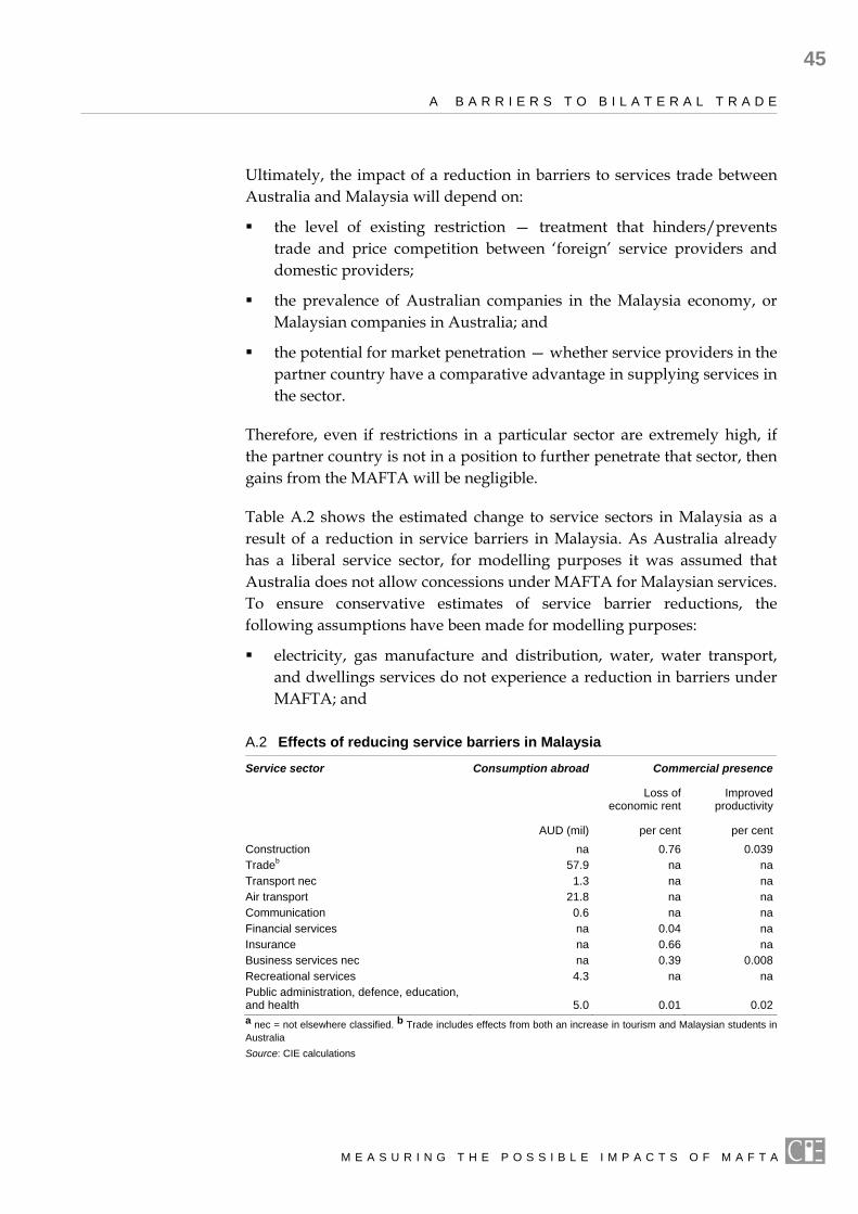
A B A R R I E R S T O B I L A T E R A L T R A D E
45
Ultimately, the impact of a reduction in barriers to services trade between Australia and Malaysia will depend on:
the level of existing restriction — treatment that hinders/prevents trade and price competition between ‘foreign’ service providers and domestic providers;
the prevalence of Australian companies in the Malaysia economy, or Malaysian companies in Australia; and
the potential for market penetration — whether service providers in the partner country have a comparative advantage in supplying services in the sector.
Therefore, even if restrictions in a particular sector are extremely high, if the partner country is not in a position to further penetrate that sector, then gains from the MAFTA will be negligible.
Table A.2 shows the estimated change to service sectors in Malaysia as a result of a reduction in service barriers in Malaysia. As Australia already has a liberal service sector, for modelling purposes it was assumed that Australia does not allow concessions under MAFTA for Malaysian services. To ensure conservative estimates of service barrier reductions, the following assumptions have been made for modelling purposes:
electricity, gas manufacture and distribution, water, water transport, and dwellings services do not experience a reduction in barriers under MAFTA; and
A.2 Effects of reducing service barriers in Malaysia
Service sector Consumption abroad Commercial presence
Loss of
economic rent Improved
productivity
AUD (mil) per cent per centConstruction na 0.76 0.039Tradeb 57.9 na naTransport nec 1.3 na naAir transport 21.8 na naCommunication 0.6 na naFinancial services na 0.04 naInsurance na 0.66 naBusiness services nec na 0.39 0.008Recreational services 4.3 na naPublic administration, defence, education, and health 5.0 0.01 0.02a nec = not elsewhere classified. b Trade includes effects from both an increase in tourism and Malaysian students in Australia Source: CIE calculations
M E A S U R I N G T H E P O S S I B L E I M P A C T S O F M A F T A

46
A B A R R I E R S T O B I L A T E R A L T R A D E
for modelling purposes a reduction in barriers to cross border supply and movement of natural persons have been captured in estimating the reduction in barriers to commercial presence and in the sensitivity analysis carried out on the reduction in service barriers.
The following outlines the procedures used in estimating a reduction in consumption abroad and commercial presence barriers for each relevant GTAP service sector in Malaysia.
Given the availability of detailed statistics, an alternative approach has been adopted for estimating the effects of liberalising those sectors where trade is (predominantly) via consumption abroad — that is, tourism and education. The approach taken is to estimate/derive the actual increase in exports as a result of the trade liberalisation, as opposed to estimating a ‘tariff equivalent’ of the barrier(s) and then removing that tariff (as has been done for estimating a reduction in barriers to commercial presence).
This approach was adopted only for Australian exports of education and tourism services via consumption abroad. Due to Australia’s already open education and tourism service trade, a change in Malaysia’s exports of education and tourism services via consumption abroad were not examined.
Tourism
Malaysia was Australia’s 9th largest source of overseas visitors in 2003, with over 155 600 short-term visitors (ABS 2004).1 Of these, 9 per cent (14 000) were business travellers, 18 per cent (28 000) visited Australia for edu-cation, employment or other (not stated) purposes, with the remaining 73 per cent (113 600) being classified as tourists (Tourism Australia 2004a).
With the average Malaysian tourist spending 11 days in country and spending $2250 per visit on average, Australia’s exports of tourism services to Malaysia is estimated to amount to over $256 million in 2003 (CIE calculations based on Tourism Australia (2004b) data). The $256 million comprises expenditure by Malaysian tourists in Australia on food, drink and accommodation, airfares, shopping, entertainment, tours etc.
A trade agreement with Australia is likely to see an increase in Malaysian tourists visiting Australia, driven in part by official recognition of Australia as a trading partner of Malaysia, deeper cultural linkages and closer ties,
1 Short-term visitors are defined as overseas visitors whose intended stay in
Australia is 12 months or less.
M E A S U R I N G T H E P O S S I B L E I M P A C T S O F M A F T A

A B A R R I E R S T O B I L A T E R A L T R A D E
47
and ‘head turning effects’. The question then turns to ‘by how much will Australia’s tourism exports to Malaysia increase under a trade agreement?’
Table A.3 shows the Australian market share of the competitive set for tourists originating from other countries within the region over the period 1999–2003. (The competitive set includes those other countries that the Australia tourism sector is competing with for tourists. For example, in the case of Malaysian tourists, the competitive market set includes Australia, New Zealand, the United States, the United Kingdom etc.) As can be seen, Australia’s market share of Malaysian tourism imports (from the com-petitive set countries) has averaged only 9.3 per cent over the last 5 years. This market share is low relative to the results achieved in other countries within the region.
In estimating the increase in tourism exports to Malaysia resulting from a trade agreement, it has been assumed that Australia captures a share of tourism imports from competitive set countries comparable to that achieved in Thailand over the last 5 years. Thailand was chosen due to its close proximity to Malaysia and similarities in per capita GDP. Hence instead of Australia capturing 10 per cent of the Malaysian competitive set market, Australia captures 13.4 per cent of the market under a trade agree-ment. This equates to an additional 38 000 Malaysian tourists visiting Australia, generating an additional $86 million in tourism related exports to Malaysia.
The $86 million increase in tourism related exports to Malaysia is spread across several GTAP services sectors, including:
Trade (restaurants, accommodation, shopping etc) — increase in exports to Malaysia of $52 million;
Transport — increase in exports to Malaysia of $28 million;
Communication — increase in exports to Malaysia of $1 million; and
Recreation — increase in exports to Malaysia of $5 million.
A.3 Captured market share of the competitive set
Tourists originating from 1999 2000 2001 2002 20035 yr
average
Per cent Per cent Per cent Per cent Per cent Per centHong Kong 10.0 10.9 10.9 10.6 10.1 10.5Japan 5.7 5.4 5.7 5.8 6.5 5.8Malaysia 7.7 7.5 10.8 12.1 10.0 9.3Singapore 16.5 13.2 17.0 14.8 21.0 16.0Thailand 13.5 13.2 14.2 12.6 13.4 13.4Source: Tourism Australia (various ‘Market Snapshot’ publications).
M E A S U R I N G T H E P O S S I B L E I M P A C T S O F M A F T A

48
A B A R R I E R S T O B I L A T E R A L T R A D E
The estimated increase in tourism related exports are based on observed expenditure patterns of Malaysian tourists visiting Australia in 2003 (see Tourism Australia (2004b) for expenditure patterns).
Public administration, defence, education and health
There are significant barriers throughout public administration, defence, education and health sectors of the Malaysian economy. The most significant of these for Australia concern education, due to Australia’s comparative advantage in this industry.
Malaysia is a key market for Australian education services. Exports of educational services to Malaysia, as measured by balance of payments data, were A$412 million in 2003, with Malaysia the fifth largest source of students coming to Australia. There are also a substantial number of Malaysian students studying in institutions in Malaysia which have links to Australian educational providers.
However, there are significant barriers to this trade. Limited recognition of qualifications by the Malaysian Public Services Department (JPA) is a significant problem. It affects not only those with Australian qualifications who wish to enter the public service in Malaysia, but may influence recognition by some private organisations. The JPA currently recognises qualifications on a course-by-course basis and on a needs-required basis. There are also significant problems with the recognition of distance education.
A particular issue for Australia relates to Australian honours degrees. The Australian honours degree (a four year degree with a research component) is only considered comparable to a pass degree or mainstream bachelor degree from European countries such as the UK.
In addition, there are significant barriers to commercial presence. Foreign universities can only set up a campus in Malaysia if they are invited by the Minister for Higher Education. Current regulations imposed on branch campuses by the National Accreditation Board (Lembaga Akreditasi Negara - LAN) limits the range of courses that can be offered. They also require courses to be offered in Bahasa, Malays and Malaysian Studies (Civics), Islamic or moral studies in a format approved by the LAN. It should be noted that LAN imposes a mandatory requirement on all private higher education institutions to offer these courses. Difficulties in obtaining visas for foreign staff add significantly to the costs of foreign universities operating in Malaysia. Furthermore, foreign educational institutions must enrol a minimum of 10 per cent of foreign students (although this is not
M E A S U R I N G T H E P O S S I B L E I M P A C T S O F M A F T A

A B A R R I E R S T O B I L A T E R A L T R A D E
49
considered an issue as Branch campuses have no difficulty in reaching this minimum).
However, there is already an Australian commercial presence in Malaysian higher education. Three Australian universities (Monash, Curtin and Swinburne) have campuses in Malaysia, and there are a number of other institutions that have twinning or franchising arrangements with counterpart institutions. Initial twinning programs have evolved into full degree programs where a Malaysian private college is franchised by a foreign university to conduct the entire program in Malaysia, with students obtaining a degree from the foreign partner university. The foreign university is responsible for all aspects of quality assurance of the program conducted in Malaysia.
Quantitative assessments of barriers to educational services for Malaysia are limited. Hoekman’s (1995) original paper on barriers to services trade assigned Malaysia a tariff equivalent of 50 per cent – the benchmark for the most restrictive tariff in this sector based on the absence of any GATS commitments. These estimates were used in subsequent work by Brown and others (1995). More detailed estimates of restrictiveness indices in this sector for a number of countries, including Malaysia, were prepared as part of research on services barriers undertaken by the Productivity Commission and have been published in Nguyen-Hong and Wells (2003).
Health
Hoekman’s estimate for Malaysia’s barriers in this sector was the maximum of 50 per cent tariff, reflecting the absence of any GATS commitments by Malaysia. Australia’s principal trading interest in this sector in the longer term probably lies in encouraging increased use of Australian specialist medical personnel by Malaysians (though consumption abroad). For modelling purposes it has been assumed that there will not be a reduction in health service barriers under MAFTA.
Public Administration and Defence
This sector is largely closed to foreign participation. Hoekman’s benchmark tariff of 200 per cent for the most heavily protected sectors (such as coastal shipping subject to cabotage) may be relevant to this sector. It has been assumed that there will be no changes in public administration and defence service barriers under an MAFTA between Australia and Malaysia.
M E A S U R I N G T H E P O S S I B L E I M P A C T S O F M A F T A

50
A B A R R I E R S T O B I L A T E R A L T R A D E
Overall Estimates for this Sector
Overall estimates for this GTAP sector are set out in table A.4. These have been derived using the following methodology:
Consumption abroad: Under a MAFTA, it is possible that there would be some improvement in key barriers to trade in this sector, for example, in areas such as recognition of Australian qualifications and courses. Anecdotal evidence from industry consultation suggests that as a conservative estimate there may be a modest expansion of Malaysia’s demand for Australian educational services as a result of the MAFTA of approximately four per cent or $5 million2 (as shown in table A.2). In addition it has been assumed that this increase in Malaysian students in Australia generates an additional consumption of trade of around $13.9 million, based on a ratio of $2.80 spent on trade to every $1 spent on education (calculated from service data obtained from the Australian Bureau of Statistics).
Commercial Presence: Based on the restrictiveness indices in Nguyen-Hong and Wells (2003) and using qualitative information from industry consultations, it was conservatively assumed that service barriers impose an additional 6.3 per cent increase in costs for Australian institutions in the higher education sector and a rent increase of approximately 12 per cent.
To obtain estimates for the GTAP sector as a whole, it is necessary to adjust the estimates of the impact on Australian higher education institutions downward by two factors
- the significance of Australian institutions with a commercial presence in the higher education sector, and
- the significance of higher education in this GTAP sector as a whole.
The significance of Australian institutions with a commercial presence was proxied by using the share of students taking Australian courses in higher education in Malaysia as a proportion of all higher education students. The number of students studying at Monash, Swinburne, and Curtin campuses in Malaysia is around 4950, compared with 575 000 students in higher education in Malaysia. However, there are a substantial number of students studying in twinning arrangements. Moreover, Curtin’s campus is designed to accommodate 3 500 students and Monash is expanding its operations, including a new medical school. For modelling purposes, we have used a factor of 3.5 per cent.
2 This refers to an increase in education expenditure over and above that would
have otherwise occurred in the absence of MAFTA.
M E A S U R I N G T H E P O S S I B L E I M P A C T S O F M A F T A

A B A R R I E R S T O B I L A T E R A L T R A D E
51
The significance of higher education in the GTAP sector as a whole was assumed to be 10 per cent. This was derived by multiplying the portion of education output within the GTAP sector by the portion of higher education within the education sector. For modelling purposes we assumed that there is a one third reduction in additional rents and costs for Australian institutions under an MAFTA.
A.4 Impacts on public administration, defence, education and health
Loss of economic rent Loss of productivity
per cent per centBefore MAFTA 50.75 6.30After MAFTA 50.74 6.2996Percentage change 0.03 0.0068a Tax equivalent measures also includes restrictions on public administration, defence and health. Loss of productivity relates to higher education only Source: CIE and DFAT calculations
Construction
Commercial presence is the principal means of delivering construction services, although construction may also require the temporary movement of specialist personnel (including engineers, architects and the like).
Malaysia’s GATS Schedule indicates that general construction work can only occur through a representative office, regional office, or locally incorporated joint-venture corporation with Malaysian interests, with the aggregate foreign shareholding not to exceed 30 per cent. There are no specific bindings on mode 4 access (except those that apply generally under Malaysia’s horizontal commitments). However, commitments may apply under other headings.
Australia has a major presence in the Malaysian industry with approximately 16 Australian subsidiaries operating in building and construction. These include a subsidiary of Bovis Lend Lease, which has operated in Malaysia since 1981 and has managed construction of a number of major projects, including the KLCC Twin Towers and support facilities for Malaysia Airlines at Kuala Lumpur International Airport. Other firms operating in the market include subsidiaries of Leighton Holdings Ltd and Multiplex Constructions Pty Ltd. Leighton claims to be recognised as the leading international contractor operating in Malaysia.
There has only been a limited amount of quantitative work on this sector. Hoekman (1995) assigned Malaysia a tariff equivalent in this sector of 10 per cent (compared to the benchmark tariff of 40 per cent under no GATS commitments). Holmes and Hardin (2000), however, assigned construction
M E A S U R I N G T H E P O S S I B L E I M P A C T S O F M A F T A

52
A B A R R I E R S T O B I L A T E R A L T R A D E
an index of restrictiveness of 0.775 (out of a possible maximum of 1) for foreign direct investment, indicating very high barriers. Both the Holmes and Hardin estimate and Hoekman’s benchmark of 40 per cent has been used in estimating the scale of rent increasing and productivity losses in this sector.
The restrictions in place in Malaysia may be expected to increase both rents in the sector and firm costs. (The Malaysian Construction Industry Master Plan Framework launched on 22 September 2004 acknowledges low productivity in the industry, which Malaysia is seeking to develop, along with education and health services as a services export industry). In the absence of direct evidence, it has been assumed that one fifth of the Holmes and Hardin estimate is cost increasing, and four fifths rent increasing.
Anecdotal evidence suggests foreign firms account for a large portion of construction output. However, as there is no strong statistical data on how significant foreign firm are in the Malaysian industry, it has been assumed that foreign firms own a total of 30 per cent of the Malaysian construction industry. This represents the maximum equity foreign firms are allowed to own. Within this, it is assumed that Australian firms account for approximately two per cent of Malaysian construction output.
For modelling purposes it has been assumed that changes under the MAFTA are assumed to lead to a third reduction in the economic rents and estimated productivity losses faced by Australian firms as a result of Malaysian barriers placed on foreign firms. Table A.5 shows the loss in economic rent and productivity due to service barriers faced by domestic and foreign firms and the impacts of MAFTA on reducing these measures.
A.5 Service barriers and post MAFTA impacts for Malaysian construction
Loss of economic rent Loss of productivity
per cent per centBefore MAFTA 25.19 6.200After MAFTA 24.99 6.198Percentage change 0.76 0.039
Source: CIE and DFAT calculations
Financial services
Restrictions to financial services in Malaysia have been significant. The most important affect commercial presence (mode three), but there are severe restrictions affecting Modes one, two and four. Mode four restrictions affect commercial presence operations.
M E A S U R I N G T H E P O S S I B L E I M P A C T S O F M A F T A

A B A R R I E R S T O B I L A T E R A L T R A D E
53
Malaysia’s 1998 GATS Schedule for Financial Services includes extensive market access restrictions and limitations on national treatment. 13 wholly foreign-owned commercial banks are allowed to remain under foreign ownership. Otherwise, foreign equity for commercial and merchant banks is limited to participation in Malaysian-owned or controlled banks, with a 30 per cent maximum foreign equity limit. Equity participation of 5 per cent of more is subject to approval on the basis of criteria set out in the schedule. For banks, mode 4 entry is limited to two senior managers for each institution with an aggregate foreign shareholding greater than 50 per cent. Up to five specialists of specified classes are permitted for each institution. Other limits apply to representative offices. There are also a number of market access limitations that apply to both domestic and foreign owned institutions.
Malaysia has been seeking to undertake progressive liberalisation of the financial services sector through a staged process of reforms. These reforms are outlined in the Financial Sector Master plan (FSM) and the Capital Market Master plan (CMM), which were released in 2001. There remains some opacity in the implementation timetables for FSM and CMM reform. There is a possibility that Mode 4 quotas applying to the number of expatriate senior managers and specialists are to be ‘uplifted’ as part of the FSM.
Australian Banks are represented to only a limited degree in Malaysia. ANZ is the most prominent banking player although is relatively small compared to other foreign banks in the Malaysian market. Furthermore, an Australian affiliate of Macquarie Bank Ltd – Macquarie (Malaysia) Sdn Bhd, has operated a representative office in Malaysia since 1996, and the National Australia Bank has had a representative office in Kuala Lumpur since 1984 and a branch in the Labuan Offshore Financial Centre.
There has been some quantitative work in this area. Hoekman (1995) estimated a “tariff equivalent” for financial services other than banking for Malaysia of 27.1 per cent (compared to the benchmark of 50 per cent with no GATS commitments). McGuire and Schuele (2000) estimated foreign and domestic restrictiveness indices for domestic banks and subsidiaries of foreign banks which put Malaysia in a highly restrictive category in each class: the foreign restrictiveness index, measuring barriers to foreign banks, was 0.65 (out of a maximum possible score of 1) and the domestic restrictiveness index 0.27 (again out of a maximum score of 1).
The McGuire and Schuele (2000) indices were used by Kalirajan et al (2000) to estimate the impact of restrictions on the price of banking services – as measured by the net interest rate margins of banks. Their finding suggested
M E A S U R I N G T H E P O S S I B L E I M P A C T S O F M A F T A

54
A B A R R I E R S T O B I L A T E R A L T R A D E
that the effect of non-prudential restrictions on all banks in Malaysia increased prices of banking services by 21.9 per cent, and that of non-prudential restrictions on foreign banks increased prices of banking services by 60.6 per cent.
For modelling purposes it has been assumed that there is a modest probability that Australian banks would utilise greater access under a MAFTA. It is likely that Australian banks would expand primarily through increased business with Australian firms in Malaysia and with Malaysian companies that deal extensively in Australia.
Table A.6 shows estimates of service barriers in Malaysia and post MAFTA impacts on the Malaysian finance industry, based on Kalirajan et al (2000). It is assumed that foreign firms account for approximately 25 per cent of equity within the finance industry (UK Trade and Investment, 2004) and within this, Australian banking firms account for approximately 0.1 per cent of total banking output in Malaysia. It is also assumed for modelling purposes that any liberalisation under the FTA would reduce the economic rents to Australian financial services firms as a result of foreign restrictions by a third.
A.6 Service barriers and post MAFTA impacts for the finance industry
Loss of economic rent Loss of productivity
per cent per centBefore MAFTA 31.59 naAfter MAFTA 31.58 naPercentage change 0.04 na
Source: CIE and DFAT calculations
Insurance
There are significant barriers to access in Malaysian insurance services. The most important of these affect commercial presence (mode 3), but there are other important restrictions affecting other modes of supply. Mode 4 restrictions also affect commercial presence.
Branches of foreign insurance companies were required to incorporate locally under Malaysian law by 30 June 1998, although the Malaysian government has granted individual extensions. Foreign shareholding exceeding 49 per cent is permitted only with Malaysian government approval but this cap was increased to 51 per cent as part of the 1997 WTO Financial Services Agreement. New entry by foreign insurance companies is limited to equity participation in locally incorporated insurance companies and aggregate foreign shareholding in such companies may not
M E A S U R I N G T H E P O S S I B L E I M P A C T S O F M A F T A

A B A R R I E R S T O B I L A T E R A L T R A D E
55
exceed 30 per cent. This limit has, however, been subject to negotiation. Restrictions on insurance cross-shareholdings of 5 per cent or more may apply to both foreign and domestic insurance companies.
Restrictions on the sale of insurance products are scheduled to be removed as part of the Financial Sector Master Plan (FSM). The pricing of general insurance products, notably fire and motor insurance products, is to be deregulated and the reinsurance industry is to be opened fully to foreign competition.
There is very limited information on quantifying the service barriers in the insurance sector. Hoekman (1995) provides an estimate of 200 per cent as a tariff equivalent for the life insurance sector for Malaysia, which represents the benchmark barrier indicating no commitments for this sector. Holmes and Hardin (2000) estimated a restrictiveness index for foreign direct investment in the insurance and related industries of 0.6 (out of a possible maximum of 1), indicating very high level of restrictions. This was similar to the level of restrictiveness they estimated for banking and other financial services (0.617).
Despite the barriers, there is a significant foreign presence in the Malaysian insurance market. According to the WTO Secretariat, 23 of 63 insurers in Malaysia were foreign owned, with foreign shares accounting for 72 per cent and 36 per cent of the total life and general premium insurance market for 2000.
There is one Australian affiliate – QBE-MBF Insurans Berhad – operating in Malaysia, According to the Austrade Directory of Business in Malaysia, it underwrites “most classes of commercial lines, personal lines and liability insurance products”. But it is a small player in the Malaysian insurance industry. Gross premium income for 2003 was slightly under 116 million ringgit, possibly around 2 per cent of the total market (general insurance premiums for Malaysia in 2000 were some 5057.9 million ringgit according to the WTO Secretariat).
The extensive foreign presence in Malaysian insurance and the limited share of the only Australian affiliate currently operating in the industry suggests that any liberalisation of commercial presence under an MAFTA would have a limited impact.
Estimating any impact is difficult. There are no estimates of the extent to which restrictions in the insurance sector raise the prices of insurance services or increase costs. In the case of banking services, however, estimates by Kalirajan et al (2000) suggest that the combined effect of domestic and foreign restrictions might be to increase net interest margins
M E A S U R I N G T H E P O S S I B L E I M P A C T S O F M A F T A
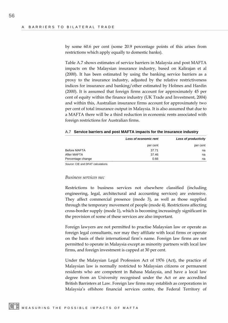
56
A B A R R I E R S T O B I L A T E R A L T R A D E
by some 60.6 per cent (some 20.9 percentage points of this arises from restrictions which apply equally to domestic banks).
Table A.7 shows estimates of service barriers in Malaysia and post MAFTA impacts on the Malaysian insurance industry, based on Kalirajan et al (2000). It has been estimated by using the banking service barriers as a proxy to the insurance industry, adjusted by the relative restrictiveness indices for insurance and banking/other estimated by Holmes and Hardin (2000). It is assumed that foreign firms account for approximately 45 per cent of equity within the finance industry (UK Trade and Investment, 2004) and within this, Australian insurance firms account for approximately two per cent of total insurance output in Malaysia. It is also assumed that due to a MAFTA there will be a third reduction in economic rents associated with foreign restrictions for Australian firms.
A.7 Service barriers and post MAFTA impacts for the insurance industry
Loss of economic rent Loss of productivity
per cent per centBefore MAFTA 37.71 naAfter MAFTA 37.46 naPercentage change 0.66 na
Source: CIE and DFAT calculations
Business services nec
Restrictions to business services not elsewhere classified (including engineering, legal, architectural and accounting services) are extensive. They affect commercial presence (mode 3), as well as those supplied through the temporary movement of people (mode 4). Restrictions affecting cross-border supply (mode 1), which is becoming increasingly significant in the provision of some of these services are also important.
Foreign lawyers are not permitted to practise Malaysian law or operate as foreign legal consultants, nor may they affiliate with local firms or operate on the basis of their international firm’s name. Foreign law firms are not permitted to operate in Malaysia except as minority partners with local law firms, and foreign investment is capped at 30 per cent.
Under the Malaysian Legal Profession Act of 1976 (Act), the practice of Malaysian law is normally restricted to Malaysian citizens or permanent residents who are competent in Bahasa Malaysia, and have a local law degree from an University recognised under the Act or are accredited British Barristers at Law. Foreign law firms may establish as corporations in Malaysia’s offshore financial services centre, the Federal Territory of
M E A S U R I N G T H E P O S S I B L E I M P A C T S O F M A F T A

A B A R R I E R S T O B I L A T E R A L T R A D E
57
Labuan, and provide legal services in their home country laws, international law and Malaysia’s offshore corporations laws to other offshore corporations established in Labuan. Foreign lawyers and law firms are also permitted to provide legal advisory services covering categories of law identified above to clients in Malaysia through cross-border mode of service supply such as through telecommunications and similar electronic networks from their country of incorporation.
Malaysia currently recognises law degrees from fourteen of the twenty nine Australian University law schools. Fourteen of the ‘unrecognised’ law schools have submitted applications for recognition. However, the Malaysian Attorney General has indicated that he is keen to establish a common bar examination as a basis for admission to practise law in Malaysia for both national and foreign qualified law students. Australia welcomes this development provided that the eligibility criteria developed to undertake for the Bar examination does not discriminate against foreign qualified students or legal practitioners.
Foreign accounting firms are permitted to provide accounting and taxation services in Malaysia only through affiliates. All accountants who wish to provide auditing and taxation services in Malaysia must register with the Malaysian Institute of Accountants (MIA) before they can apply for a licence from the Ministry of Finance. Proof of citizenship or permanent residency is required for registration with the MIA. There is also a minimum working period before they can apply for registration (158 days).
Foreign architectural firms may operate in Malaysia only as a joint-venture participant in a specific project with the approval of the Board of Architects. Malaysian architectural firms are not permitted to have foreign architectural firms as registered partners. Foreign architects may not be licensed in Malaysia but are allowed to be managers, shareholders, or employees of Malaysian firms. Only licensed architects may submit architectural plans.
Foreign engineers may be licensed by the Board of Engineers (Board) only for specific projects, and must be sponsored by the Malaysian company carrying out the project. This licence is only valid for the duration of the project. In general, a foreign engineer must be registered in his/her home country as a professional engineer, have a minimum of 10 years experience, and have a physical presence in Malaysia for at least 180 days in a calendar year. To obtain temporary licensing for a foreign engineer, the Malaysian company must demonstrate to the Board that they are unable to find a Malaysian engineer to do the job. Foreign engineers are not permitted to operate independently to the Malaysian partners of the company, or serve
M E A S U R I N G T H E P O S S I B L E I M P A C T S O F M A F T A

58
A B A R R I E R S T O B I L A T E R A L T R A D E
as directors or shareholders of a consulting engineering company. A foreign engineering company may establish a commercial presence if all the directors and shareholders are Malaysian. Foreign engineering companies may collaborate with a Malaysian company, but the latter is expected to design the project and required to submit the plans.
In terms of quantifying these barriers, studies are limited but suggest significant barriers. Hoekman (1995) assigned Malaysia a tariff equivalent of 21.3 per cent for business services (compared to his benchmark for this sector of 40 per cent in the absence of any GATS commitments). Holmes and Hardin assigned Malaysia a restrictiveness index in this area of 0.316 for foreign direct investment (out of a maximum possible of 1).
More extensive work has been carried out by the Productivity Commission (Nguyen-Hong 2000), providing the following restrictiveness indices for Malaysia based on a number of components affecting both establishment of operations and ongoing operations (see table A.8).
A.8 Restrictiveness indices for Malaysia selected business services
Engineering Architecture Accountancy Legal
Domestic Establishment 0.08 0.04 0.04 0.04 Ongoing operations 0.01 na 0.05 0.09 Total 0.08 0.04 0.09 0.13Foreign Establishment 0.24 0.33 0.46 0.45 Ongoing operations 0.02 na 0.06 0.09 Total 0.26 0.33 0.51 0.54
Source: Nguyen Hong (2000)
This study sought to estimate the price and cost impact of engineering services by looking at margins across some 84 engineering service companies in 20 countries, including Malaysia. It found that the primary impact of foreign barriers was to raise prices rather than increase costs. For Malaysia, the price impact of all barriers to foreign service suppliers was found to be 12 per cent. Domestic barriers to establishment were found to increase costs in Malaysia by 5.3 per cent.
To obtain an estimate of the impact on various restrictions on the price of business services, Nguyen Hong’s estimates for engineering were used as a benchmark and then adjust by the restrictiveness indices which apply for legal, architecture and accountancy services. Although, Nguyen Hong did not find evidence of cost escalating effects for barriers to foreign firms, a conservative assumption of 2.5 per cent for the sector was used – roughly half the cost impact Nguyen Hong found for domestic barriers to establishment for engineering services.
M E A S U R I N G T H E P O S S I B L E I M P A C T S O F M A F T A

A B A R R I E R S T O B I L A T E R A L T R A D E
59
Through consultations between DFAT and Australian businesses, it was found that there is strong interest in some of these sectors – for example, the legal profession is interested in securing improved access to the Malaysian market. However, the extent to which major Australian firms would establish a commercial presence in the market if Australia were to secure improved access is a still uncertain.
Table A.9 shows estimates of service barriers in Malaysia and post MAFTA impacts on the Malaysian business services nec industries, based on Kalirajan et al (2000). It is assumed that foreign firms account for approximately 15 per cent of equity within the business services industries, based on anecdotal evidence from consultations between DFAT and Australian businesses. Australian business service firms are assumed to account for approximately one per cent of total business services nec output in Malaysia. As a result of MAFTA it is assumed that there will be a third reduction in economic rents and an improvement in productivity associated with foreign restrictions for Australian firms.
A.9 Service barriers and post MAFTA impacts for business services nec
Loss of economic rent Loss of productivity
per cent per centBefore MAFTA 14.52 2.50After MAFTA 14.46 2.4998Percentage change 0.39 0.008
Source: CIE and DFAT calculations
Non-tariff barriers to trade The United States Trade Representative (USTR) reports that tariffs are the main barrier used by Malaysia to control/limit imports (USTR 2004). However, Malaysia also uses non-tariff barriers (NTBs) to control imports. For example, around 17 per cent of tariff lines in the Malaysian tariff schedule are subject to non-automatic import licensing, designed to protect import sensitive or strategic industries (such as agricultural, mineral and motor vehicles) (USTR 2004).
Other NTBs used by Malaysia include the following (as identified by the USTR).
50 per cent excise tax rebate made available to the Malaysian automotive manufactures Proton and Perodua. The excise tax rebate is not made available to any other car manufacturers.
M E A S U R I N G T H E P O S S I B L E I M P A C T S O F M A F T A
60
A B A R R I E R S T O B I L A T E R A L T R A D E
The sole rice importer is a government corporation that has power to regulate rice imports and ensure that domestic rice production is purchased.
The Halal certification process is non-transparent, with each product, as opposed to a plant, requiring certification from the Islamic Centre (and on joint recommendation by the Malaysian Department of Veterinary Science and Ministry of Agriculture). Infrequent audits by Malaysian inspection teams limits the ability of new products to obtain halal certification.
Licensing restrictions on white sugar effectively blocks Australian sugar producers from exporting white sugar to Malaysia
The ability of foreign suppliers to compete for Malaysian Government procurement contracts is limited by the government’s policy for pro-curement contracts to be used to support national public policy objectives such as encouraging greater participation of ethnic Malays in the economy (Bumiputera), technology transfer, etc.
Sale of counterfeit products (such as pharmaceuticals) and piracy of copyright materials (particularly optical media products), which act to limit the ability of legitimate producers to enter the market.
Exporters to Australia typically cite Australia’s regime for the application of sanitary and phytosanitary (SPS) measures as being a NTB, which results in restrictions and prohibitions on imports of agricultural products. Some countries contend that the SPS based restrictions imposed by Australia are more trade restrictive than necessary. Other significant NTBs in Australia include the following (once again, as identified by the USTR).
Australia is not a signatory to the WTO Agreement on Government Procurement.
Adjustment assistance/support packages for the dairy and sugar industries, including interest rate subsidies and short-term income support.
Support measures for the automotive and textiles, clothing and footwear industries.
Estimating what benefit could arise through liberalisation of such NTBs first requires a judgement as to whether the measure is actually a legitimate barrier or an unwarranted trade barrier. If the latter, then the ad valorem equivalence of those trade barriers is required (that is, the NTBs need to be approximated by a tariff equivalent).
M E A S U R I N G T H E P O S S I B L E I M P A C T S O F M A F T A

A B A R R I E R S T O B I L A T E R A L T R A D E
61
Approximating the tariff equivalence of NTBs is a difficult exercise, with the required data being rarely available. What is needed is the landed price of an imported product and the ex-factory price for a comparable domestic product. Alternatively, if comparable products cannot be found, then the price of the same product exported to Malaysia and to another ‘benchmark’ region that is unprotected (such as Singapore). The price differential between the imported and local product (or between the same product exported to two different markets) once tariffs, transportation costs and any other non-discriminatory taxes are taken into account, can be attributed to NTBs (OECD 1997).
Unfortunately, such data has not been accessible. In the absence of required data, no attempt has been made to quantify the NTBs in Australia and Malaysia. To the extent that the NTBs have been overlooked, the economic benefits from Australia and Malaysia entering into a bilateral trade agree-ment as reported in this study will likely be a conservative estimate.
M E A S U R I N G T H E P O S S I B L E I M P A C T S O F M A F T A

62
B Baseline assumptions
To estimate the potential economic impacts of the FTA, an appropriate counterfactual (the ‘baseline’) needs to be established. The baseline represents the business-as-usual scenario — that is, what liberalisation can we expect to happen in the absence of the FTA. As many tariffs are scheduled to fall anyway as a result of previous commitments made else-where (for example, under the Uruguay Round of the GATT, subsequent WTO commitments, APEC and other FTAs), these commitments clearly needs to be taken account of. For example, it would be inappropriate to remove Australia tariffs on motor vehicles under the FTA and attribute all resultant outcomes as a benefit of the FTA as some of those gains will be realised irrespective of the FTA as Australia has already announced unilateral reductions in motor vehicles. Hence, establishing an appropriate baseline is a critical step in evaluating the economic implications of the FTA.
Results from the FTA simulation(s) are compared with the baseline, with the difference being attributable to trade liberalisation undertaken as part of the FTA. Model results are (typically) presented as a percentage change from the baseline outcome and, in the case of APG–Cubed, results are presented for each year until 2027.3
Multilateral and unilateral trade liberalisation
Given the recent uncertainty surrounding future rounds of the WTO, we are not in a position to speculate about further trade liberalisation on a MFN basis. Further trade liberalisation organised under the auspices of the WTO is, therefore, excluded from the baseline. The APEC liberalisations announced under the Bogor Declaration (complete unilateral trade liberalisation by 2010 for developed country members and by 2020 for developing members) are voluntary and do not have the legal force that
3 Actual model runs in APG–Cubed are much longer, extending to year 2131 for
baseline generation and year 2100 for policy simulation.
M E A S U R I N G T H E P O S S I B L E I M P A C T S O F M A F T A
B B A S E L I N E A S S U M P T I O N S
63
MFN tariff reductions have as agreed and signed under the Uruguay Round of the GATT.
Australia
The Australian Government has announced that tariff barriers in the textiles, clothing and footwear (TCF) and PMV sectors would be phased down over a number of years. PMV tariffs, currently at 10 per cent, will remain at this level until January 2010 when they will be reduced to 5 per cent and remain at this level until 2015. TCF tariffs, currently at 17.5, 10 and 7.5 per cent (respectively) will remain at this level until January 2010, when the 10 and 7.5 per cent TCF tariffs will be reduced to 5 per cent, while the 17.5 per cent tariff will fall to 10 per cent. These tariffs will be further reduced to 5 per cent in 2015 (PC 2003, p. 2.8). As the Australian Government is committed to these tariff reductions, they have been included in the baseline.
Malaysia
There are no multilateral tariff reductions scheduled for Malaysia
Bilateral trade liberalisation
Bilateral agreements entered into after the reference year for the underlying database (2003) were included in the baseline (the effects of trade agreements entered into prior to 2003 will be picked up in the database).
Australia
Australia currently has FTAs with New Zealand (entered into in 1983) and, more recently, Singapore (2003). In 2004, Australia signed a bilateral free trade agreements with Thailand and the United States, which both entered into force at the start of January 2005. These agreements comprise merchandise trade, service and investment liberalisation. As both agreements have been approved by the Australian Government, they have been included in the baseline.
Recent talks between Australia/New Zealand and ASEAN on a free trade agreement have not been included in the baseline, nor have Australia and China’s current free trade agreement talks.
M E A S U R I N G T H E P O S S I B L E I M P A C T S O F M A F T A

64
B B A S E L I N E A S S U M P T I O N S
Malaysia
Malaysia is part of the ASEAN Free Trade Area (AFTA), which is a collective effort by ASEAN members to substantially reduce or eliminate tariffs on intra-ASEAN trade in the merchandise sector. As a consequence, the AFTA has been included in the baseline.
As part of its ASEAN membership, Malaysia has also been involved in negotiations on free trade agreements between ASEAN and India, and ASEAN and China. The trade agreement between ASEAN and India has been excluded from the baseline due to uncertainty about when the trade agreement will enter into force, and the coverage and timing of liberalisation.
In November 2002, ASEAN and China agreed on an Early Harvest Program as one component of a broader Framework Agreement on cooperation. For the six older ASEAN economies and China, this required tariffs (other than those exempted) between Chapters one to eight of the HS code to be reduced to zero by dates between 2004 and 2006 (depending on the level of initial tariff). As these tariff reductions have been agreed upon by ASEAN members, they have been included in the baseline, along with specific products not in chapters one to eight that have also been included in the early harvest program by each ASEAN member and China. In late November, ASEAN and China also reached an agreement on preferential reductions on trade in goods not included in the Early Harvest Program but at the time of writing the schedules had not been released to the public. Therefore they have not been included in the baseline.
Malaysia also started negotiating a trade agreement with Japan in January 2004. As there have not been any definitive outcomes it has not been included in the analysis. Furthermore, free trade discussions between ASEAN and Japan and ASEAN and Korea have not been included.
Trade liberalisation under the FTA Australia and Malaysia have a vast range of FTA implementation scenarios at their disposal. For example, trade barriers could either be completely or partially eliminated, the FTA could be implemented immediately or phased in over 5 or 10 years, both goods and services could be covered, or just goods, and so on. Furthermore, both countries need not adopt the same trade liberalisation schedule.
M E A S U R I N G T H E P O S S I B L E I M P A C T S O F M A F T A
B B A S E L I N E A S S U M P T I O N S
65
It is assumed that Australia and Malaysia enter into the FTA in 2007. The trade liberalisation scenarios considered for the purpose of estimating the possible economic impacts of the FTA comprise:
immediate elimination of all barriers to trade in 2007;
phased elimination of all barriers to trade over a 5 year period, with trade liberalisation starting in 2007 and free trade achieved by 2011; with trade barriers being removed in 5 equal instalments; and
phased elimination of all barriers to trade over a 10 year period, with trade liberalisation starting in 2007 and free trade achieved by 2016; with trade barriers being removed in 10 equal instalments.
The barriers to trade removed under the Agreement are those identified in tables A.1 (tariff barriers), and A.2 (service barriers) of appendix A. Dynamic productivity improvements, as shown in table C 2 of appendix C are assumed to accrue in line with the trade liberalisation.
M E A S U R I N G T H E P O S S I B L E I M P A C T S O F M A F T A

66
C Dynamic productivity
GLOBAL GENERAL EQUILIBRIUM economic models, such as GTAP and APG–Cubed, are typically used to quantify the economic impacts of trade liberalisation. However, examination of the models’ predicted changes in growth and trade flows against observed changes leads to the observation that economic models tend to under predict the growth/trade changes resulting from trade liberalisation. The current thinking is that economic models under predict the changes associated with trade liberalisation due to ignoring effects related to productivity linkages, pro-competitive effects and investment dynamics (Itakura, Hertel and Reimer, 2003). These effects have been termed the ‘dynamic productivity’ effects of trade liberalisation.
Dynamic productivity An increase in openness to trade is thought to promote productivity increases and growth within a country through an improvement in the efficiency with which resources are allocated, the stimulation of innovation, and the transfer of knowledge and technology between countries. Hence there are two types of gain associated with trade liberalisation — allocative efficiency gains and dynamic productivity gains.
It is generally accepted that countries can achieve allocative efficiency gains through trade liberalisation. These gains are improvements in the level of output and productivity from the reallocation of resources to the more productive/efficient sectors of the economy. Allocative gains represent the traditional theory on the benefits from trade liberalisation. Consequently, it is these gains are typically estimated and reported.
However, trade reform also sees an increase in import competition, thereby encouraging domestic producers to pursue productivity gains, either though the use of better technology and business practices, or through innovation and/or quicker adoption of new ideas. Improved domestic efficiency and liberalisation of other countries’ trade barriers will improve the competitive position of exporters, and greater exports may also be associated with productivity gains. There can be learning by exporting
M E A S U R I N G T H E P O S S I B L E I M P A C T S O F M A F T A

C D Y N A M I C P R O D U C T I V I T Y
67
where the experience and knowledge gained in export markets can be translated into productivity gains (Aw, Chung and Roberts 2000). Ex-porting may also allow producers to expand output and exploit economies of scale, thereby lowering average production costs (Itakura, Hertel and Reimer, 2003).
Finally, a ‘more efficient’ economy will likely open the way for new foreign investment opportunities leading to transfer of technical know-how and capital accumulation, which can inturn stimulate productivity growth and lead to higher economic growth.
Improvements to efficiency due to improved work practices (as opposed to resource re-allocation) are referred to as dynamic productivity gains. The literature on dynamic efficiency gains from trade openness is not as robust compared to that on allocative gains, and consequently these types of gains are often excluded from trade policy analysis. However, researchers are now turning their attention to the issue of dynamic productivity, and a number of econometric studies have found a relationship between import competition, exporting and foreign investment and productivity growth (see, for example, Itakura, Hertel and Reimer (2003) and Wacziarg (2001)). If dynamic gains are important and they are not considered in modelling economic effects from trade liberalisation, then excluding dynamic gains may understate the net benefits.
There is, however, current debate on whether a reduction in trade barriers actually increases productivity and growth. Although a number of studies have found a positive relationship between trade openness and growth, some economists have been sceptical of the econometric results. According to Edwards (1998), two issues have been at the core of these controversies — until recently, theoretical models had been unable to link trade policy to faster equilibrium growth, and secondly, the empirical literature on the subject has been affected by serious data problems. These include generating satisfactory indexes to measure trade policy orientation, and the specification of equations used to measure direct relationships between trade policy and growth.
The relationship between trade policy and economic productivity and growth is therefore debatable. As Rodriguez and Rodrik (1999) have noted,
Our bottom line is that the nature of the relationship between trade policy and economic growth remains a very much open question. The issue is far from having being settled on empirical grounds.
We suspect that the relationship is a contingent one, dependent on a host of country and external characteristics. (Rodriguez and Rodrik 1999, p. 4)
M E A S U R I N G T H E P O S S I B L E I M P A C T S O F M A F T A

68
C D Y N A M I C P R O D U C T I V I T Y
Despite this debate, there is, however, substantial anecdotal evidence of the existence of dynamic productivity gains. For example, since deep tariff cuts in the mid 1980s–90s, enterprises in Australia’s manufacturing sector have tripled their spending on research and development (as a proportion of turnover), raised capital per employee by 33 per cent, improved product quality and response times (Roberts 2004).
Due to the debate (amongst economists) surrounding the legitimacy of dynamic productivity gains, the effects of such gains are reported separately in chapters five and six. This allows the reader to include or exclude the gains from dynamic productivity as they see fit when estimating the total economic impact of a bilateral trade agreement between Australia and Malaysia.
Where can dynamic gains come from?
Most previous empirical models of trade have excluded the impacts an increase in competition can have on productivity throughout time. These are referred to as ‘static’ models. According to the World Bank, recent empirical models have extended their analysis from static allocative efficiency type gains to measuring dynamic gains along four main research paths (WB 2002)
Dynamic investment — As tariffs are often imposed on investment goods, a reduction in trade barriers on these goods can lead to an increase in the return to capital and therefore a rise in real investment and productivity. Higher incomes from increased productivity lead to higher savings and thus further capital accumulation.
Pro-competitive effects and scale economies — An increase in foreign competition can have disciplinary effects on domestic mark-ups by reducing the market power of domestic firms. Furthermore, the ability to increase market size through greater exports allows domestic firms to reduce their average cost by introducing more specialised equipment and bulk-handling methods, thereby increasing productivity on the factory floor.
Endogenous productivity — Only those foreign firms with relative productivity efficiencies will expand into a domestic market. Con-sequently, local firms may take advantage of new technologies, innovations, and production methods introduced into the economy from foreign firms to enhance their own productivity.
Endogenous capital flows — There is significant empirical evidence that gains from international capital mobility are quantitatively important. Foreign direct investment from abroad may bring new and improved
M E A S U R I N G T H E P O S S I B L E I M P A C T S O F M A F T A

C D Y N A M I C P R O D U C T I V I T Y
69
technologies that could flow into the domestic economy and increase market productivity.
The size of any dynamic productivity gains for Australia and Malaysia arising from bilateral trade liberalisation will ultimately depend upon:
the linkages between competition, innovation, and productivity within the economy;
the relative sectoral efficiencies that already exist between Australia and Malaysia;
the size of the change in competition;
the type of market and the ownership structure in the domestic industries; and
the ability of domestic firms to incorporate innovation and production techniques.
A measure of the impacts of trade liberalisation on productivity can be estimated by investigating recent empirical studies on the effects of trade liberalisation on domestic and international markets.
The importance of dynamic gains
There have been a number of global trade simulations that have included dynamic productivity gains, including studies by the World Bank and OECD (WB 2002). Comparing the gains from full trade liberalisation from a selected number of studies shows static efficiency gains have been magnified (WB 2002).
There has been an increasing amount of effort employed by economists in an attempt to determine the size of the link between competition and dynamic productivity growth. Table C.1 shows the outcomes of a range of studies where reductions in various trade barriers have been associated with an increase in dynamic productivity and growth.
M E A S U R I N G T H E P O S S I B L E I M P A C T S O F M A F T A

70
C D Y N A M I C P R O D U C T I V I T Y
C.1 Selected empirical studies finding dynamic gains from reduced trade protection
Study Country Sector Year Results
Chand (1999) Australia Manufacturing 1967–95 A 1 per cent reduction in nominal rate of assistance produces a 0.18 to 0.50 per cent increase in total factor productivity
Chand and Vousden (1996)
Australia Manufacturing 1970-91 A 1 per cent increase in an independent measure of assistance led to a 0.3 per cent decline in manufacturing industry output
Ianchovichina et al (2000) Australia Automotive 1968–75 A 1 per cent reduction in automotive tariffs produces a 0.36 per cent increase in foreign competition
Frankel and Romer (1999) 63 countries Across all sectors
1985 Increasing the ratio of trade to GDP by 1 per cent raises income per person by between 0.5 and 2 per cent
MacDonald (1994) US Manufacturing 1972–87 A 5 per cent increase in market import share is associated with a 3.7 per cent increase in annual labour productivity growth for highly concentrated industries
Chuang and Lin (1999) Taiwan Manufacturing 1991 A 1 per cent increase in FDI produces a 1.4 to 1.88 per cent increase in domestic firm productivity
For the purposes of this analysis, we have used the results from the first two of the studies shown in table C.1 — which are recent Australian studies. In the absence of studies specifically relating to Malaysia, it has assumed that there exists a similarity between Australian and Malaysian manufacturing.
The average relationship between a tariff reduction and an increase in productivity in manufacturing from the first two studies suggests that a 1 percentage point unilateral reduction in tariffs in manufacturing sectors will result in an approximate 0.3 per cent increase in productivity. To estimate the expected dynamic productivity gain in Australian and Malaysian manufacturing, this impact was multiplied by the reduction in tariffs for each sector under the trade agreement. The gains were then adjusted for the proportion of total imports (by sector) accounted for by the other country (to reflect the fact that trade liberalisation under the trade agreement is on a bilateral basis and not multilateral). Hence the larger the tariff reduction to occur, and the larger the share of total imports of that product accounted for by imports from the other country, the larger the assumed dynamic productivity gain in that sector. This approach sees the dynamic productivity gain not depending on the absolute quantity of imports from the other country; rather, it depends (in part) on the share of total imports accounted for by the other country. The dynamic productivity gain in each sector therefore leverages off:
the size of the bilateral tariff barrier to be removed; and
the share of total imports (on a sectoral basis) accounted for by imports from the other country.
M E A S U R I N G T H E P O S S I B L E I M P A C T S O F M A F T A
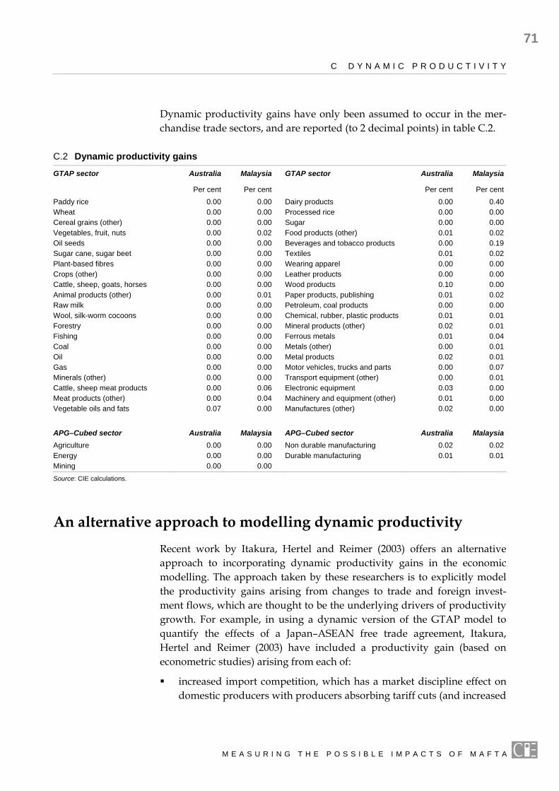
C D Y N A M I C P R O D U C T I V I T Y
71
Dynamic productivity gains have only been assumed to occur in the mer-chandise trade sectors, and are reported (to 2 decimal points) in table C.2.
C.2 Dynamic productivity gains
GTAP sector Australia Malaysia GTAP sector Australia Malaysia
Per cent Per cent Per cent Per centPaddy rice 0.00 0.00 Dairy products 0.00 0.40Wheat 0.00 0.00 Processed rice 0.00 0.00Cereal grains (other) 0.00 0.00 Sugar 0.00 0.00Vegetables, fruit, nuts 0.00 0.02 Food products (other) 0.01 0.02Oil seeds 0.00 0.00 Beverages and tobacco products 0.00 0.19Sugar cane, sugar beet 0.00 0.00 Textiles 0.01 0.02Plant-based fibres 0.00 0.00 Wearing apparel 0.00 0.00Crops (other) 0.00 0.00 Leather products 0.00 0.00Cattle, sheep, goats, horses 0.00 0.00 Wood products 0.10 0.00Animal products (other) 0.00 0.01 Paper products, publishing 0.01 0.02Raw milk 0.00 0.00 Petroleum, coal products 0.00 0.00Wool, silk-worm cocoons 0.00 0.00 Chemical, rubber, plastic products 0.01 0.01Forestry 0.00 0.00 Mineral products (other) 0.02 0.01Fishing 0.00 0.00 Ferrous metals 0.01 0.04Coal 0.00 0.00 Metals (other) 0.00 0.01Oil 0.00 0.00 Metal products 0.02 0.01Gas 0.00 0.00 Motor vehicles, trucks and parts 0.00 0.07Minerals (other) 0.00 0.00 Transport equipment (other) 0.00 0.01Cattle, sheep meat products 0.00 0.06 Electronic equipment 0.03 0.00Meat products (other) 0.00 0.04 Machinery and equipment (other) 0.01 0.00Vegetable oils and fats 0.07 0.00 Manufactures (other) 0.02 0.00
APG–Cubed sector Australia Malaysia APG–Cubed sector Australia MalaysiaAgriculture 0.00 0.00 Non durable manufacturing 0.02 0.02Energy 0.00 0.00 Durable manufacturing 0.01 0.01Mining 0.00 0.00 Source: CIE calculations.
An alternative approach to modelling dynamic productivity Recent work by Itakura, Hertel and Reimer (2003) offers an alternative approach to incorporating dynamic productivity gains in the economic modelling. The approach taken by these researchers is to explicitly model the productivity gains arising from changes to trade and foreign invest-ment flows, which are thought to be the underlying drivers of productivity growth. For example, in using a dynamic version of the GTAP model to quantify the effects of a Japan–ASEAN free trade agreement, Itakura, Hertel and Reimer (2003) have included a productivity gain (based on econometric studies) arising from each of:
increased import competition, which has a market discipline effect on domestic producers with producers absorbing tariff cuts (and increased
M E A S U R I N G T H E P O S S I B L E I M P A C T S O F M A F T A

72
C D Y N A M I C P R O D U C T I V I T Y
competition from imports) through a combination of price and output reductions rather (as opposed to output alone);
changing exports, with an increase in exports being associated with rising average productivity for the sector (exporters are assumed to be 8 per cent more efficient than domestically orientated firms); and
increases in foreign direct investment (FDI) being associated with increases in domestic firm productivity (a 1 per cent increase in FDI seeing a 1.4 per cent increase in firm productivity).
This approach differs from the approach adopted in this scoping study of basing the productivity gain on the size of the bilateral tariff being removed and the share of imports accounted for by the partner country.
The approach adopted by Itakura, Hertel and Reimer (2003) should be viewed as an initial attempt to investigate the potential impacts and importance of dynamic productivity gains when quantifying the economic impacts of trade agreements. Indeed, the authors identify several areas of required further research to refine the approach. Despite these qualifiers, the results of the Itakura, Hertel and Reimer (2003) paper can be used as a benchmark to see whether the methodology used in this study to incorporate dynamic productivity is likely to under or overstate the gains.
Table C.3 compares the results of the two approaches to incorporating dynamic productivity into the economic modelling of trade liberalisation.
C.3 Comparison of contribution of dynamic productivity to welfare gains
Indicator Share of gain due to dynamic
productivityUnderstatement of gains if
dynamic productivity excluded
Per cent Per centItakura et al
Equivalent variation ASEAN(6)a 75 300
Gross domestic product ASEAN(6)a 44 78Malaysia 53 114
Scoping study
Equivalent variation Australia 35 55Malaysia 15 18
Gross domestic product Australia 48 95Malaysia 18 23
a Contribution of dynamic productivity to the welfare gains made by the ASEAN(6) members of Indonesia, Malaysia, Philippines, Singapore, Thailand and Vietnam in aggregate. Source: Itakura, Hertel and Reimer (2003), GTAP modelling simulation and CIE calculations.
M E A S U R I N G T H E P O S S I B L E I M P A C T S O F M A F T A

C D Y N A M I C P R O D U C T I V I T Y
73
As can be seen, the methodology used by Itakura, Hertel and Reimer (2003) sees dynamic productivity accounting for a larger share of the gains in equivalent variation (welfare) and economic activity (gross domestic pro-duct). As such, excluding dynamic productivity is associated with a substantial underestimation of the welfare gains (300 per cent) and growth in economic activity (Malaysia, 114 per cent) arising as a result of trade liberalisation.
In comparison, the methodology used in this scoping study to incorporate dynamic productivity gains arising from trade liberalisation typically sees dynamic productivity accounting for a smaller share of the gains and a smaller understatement of gains if dynamic productivity is excluded. It is therefore possible to speculate that the approach used in this study sees gains being generated as a result of dynamic productivity being too low, relative to those obtained by Itakura, Hertel and Reimer (2003).
Hence if the underlying econometrics and modelling approach employed by Itakura, Hertel and Reimer (2003) is correct, then it is likely that the approach used here to model dynamic productivity will see the resultant gains being a conservative estimate. The approach employed by Itakura, Hertel and Reimer (2003) was not used in this study due the authors noting that further econometric research was needed to verify the productivity linkages/relationships.
M E A S U R I N G T H E P O S S I B L E I M P A C T S O F M A F T A

74
D Economic models used to analyse the trade liberalisation
THE ECONOMIC MODELS used to evaluate the possible economic impacts of a bilateral free trade agreement between Australia and Malaysia are outlined in this appendix.
APG–Cubed The G–Cubed Asia Pacific (APG–Cubed) model emerged from a research program designed to link two strands of quantitative economic modelling:
traditional multisectoral general equilibrium models — which capture interactions between sectors but which are often static, do not generally incorporate the financial sector and do not have full macroeconomic closure; and
macroeconomic models — which are mostly dynamic and have full macroeconomic closure but which usually do not capture intersectoral interactions and often do not have a well-specified supply side.
The origins of APG–Cubed are the MSG2 macroeconomic model (McKibbin and Sachs 1991) and the G–Cubed model. Both of these models have proved successful in a wide variety of applications.
Several features of APG–Cubed make it an ideal tool for analysing the effects of trade liberalisation with endogenous productivity and risk premiums.
With its macroeconomic detail, and integrated real and financial markets, APG–Cubed can account for the effects of a financial shock on interest rates, exchange rates and international capital movements. It can also account for the effects of different government fiscal and monetary responses to these shocks. The model fully integrates wealth effects on consumption and captures debt burdens and expectations.
M E A S U R I N G T H E P O S S I B L E I M P A C T S O F M A F T A

D E C O N O M I C M O D E L S U S E D T O A N A L Y S E T H E T R A D E
75
With its explicit treatment of expectations, APG–Cubed can account for the ways in which future policy changes that are credible can affect economic activity in the early stages of implementation.
As a global general equilibrium model, APG–Cubed accounts for the interactions between sectors and between regions. Thus, it can capture the effects of policy changes and shocks within an economy and between economies.
As a dynamic model, APG–Cubed can account explicitly for the time paths of policies and shocks.
By contrast, the comparative static modelling frameworks (such as GTAP — see below) used in traditional computable general equilibrium models do not include treatment of dynamics, interest rates, expectations or capital movements.
Country and industry coverage
APG–Cubed separately identifies 19 countries/regions and six sectors of production (see table D.1).
D.1 Economy and industry coverage of APG–Cubed
Economies Sectors Australia New Zealand Energy Canada Non-oil developing countries Mining
Agriculture China Oil exporting developing countries
Durable Manufacturing
Taiwan Rest OECD Non-durable manufacturing Hong Kong Philippines Services India Singapore Indonesia Thailand Japan United States Korea USSR and Eastern Europe Malaysia
Key features
Detailed specifications of the theoretical structure of APG–Cubed can be found in McKibbin (1996). The key features of APG–Cubed are that it:
specifies the demand and supply sides of industrialised economies;
integrates the real and financial markets of these economies;
fully accounts for stocks and flows of real resources and financial assets;
M E A S U R I N G T H E P O S S I B L E I M P A C T S O F M A F T A

76
D E C O N O M I C M O D E L S U S E D T O A N A L Y S E T H E T R A D E
imposes intertemporal budget constraints so that agents and countries cannot indefinitely borrow and lend without undertaking the resource transfers necessary to service outstanding liabilities;
has short run behaviour that is a weighted average of neoclassical optimising behaviour and liquidity constrained behaviour;
has a real side that is disaggregated to allow for production and trade of multiple goods and services within and between economies;
has full short and long run macroeconomic closure with annual macrodynamics around a neoclassical growth model; and
can be solved for the full rational expectations equilibrium annually from 2002 to 2100.
Like other models, APG–Cubed essentially consists of a theoretical frame-work, data and parameters.
Theory
The model theory consists of behavioural and accounting relationships. The model recognises a number of economic agents including firms, house-holds and government.
Firms
Each sector is represented by a firm, which chooses its inputs and level of investment so as to maximise its stockmarket value, subject to a multiple input production function and output prices (which are given as far as the firm is concerned).
Sectoral output is produced using capital, labour, energy and materials. Energy and materials are aggregates of inputs of intermediate goods, which are in turn aggregates of imported and domestic commodities that are assumed to be imperfect substitutes.
The capital stock in each sector changes according to the rate of fixed capital formation and the rate of depreciation. Investment is subject to rising marginal installation costs so that total real investment is the value of purchases plus the per unit cost of installation. The per unit cost is a function of the rate of investment. This implies that, once in place, it is costly to move physical capital between sectors. In contrast, financial capital is perfectly mobile.
M E A S U R I N G T H E P O S S I B L E I M P A C T S O F M A F T A

D E C O N O M I C M O D E L S U S E D T O A N A L Y S E T H E T R A D E
77
The goal of each firm is to choose its inputs to maximise intertemporal net (of tax) profits. Taxes included are a corporate income tax, taxes on inputs (such as a carbon tax) and an investment tax credit.
Wages
Wages are determined by assuming that labour is mobile between sectors in each region, but not between regions. Thus, each sector in a region pays the same wages. Wages in a particular country adjust according to an overlapping contracts model where nominal wages depend on current and expected inflation and on labour demand relative to labour supply. Long run labour supply is determined by the (exogenous) rate of population growth. In the short run, hours worked can fluctuate. For a given nominal wage the demand for labour determines short run unemployment in each sector. This varies, depending on the composition of demand for each sector’s output.
Households
Household behaviour is assumed to be a weighted average of two types of behaviour. In the first, households aim to maximise intertemporal utility subject to a wealth constraint. Wealth consists of human wealth and financial assets. Human wealth is the present value of the expected future stream of after-tax labour income. Financial wealth is the sum of real money balances, real government bonds, net claims against foreigners and the value of capital in each sector.
In the second type of behaviour, households base their consumption on after-tax current income.
Government
Real government spending is exogenous and constant as a share of GDP. Government consumption is financed by taxes (corporate and personal income taxes) and by issuing government debt.
The government budget must balance in present value terms but need not balance in any single period. Thus, if the government runs a budget deficit today, it must run an appropriate budget surplus at some point in the future. If not, the government will be unable to pay interest on debt and private agents will not be willing to hold it. The specific fiscal closure chosen is that at every instant in time the government must levy a lump sum tax equal to the value of interest payments on the outstanding debt.
M E A S U R I N G T H E P O S S I B L E I M P A C T S O F M A F T A

78
D E C O N O M I C M O D E L S U S E D T O A N A L Y S E T H E T R A D E
Financial markets and balance of payments
The model accounts for flows of assets between regions, consistent with the flows of goods. The model specifies that money is required to undertake transactions and so the demand for money is a function of GDP and short term nominal interest rates. The supply of money is exogenously chosen by the central bank in each region.
Asset markets are assumed to be integrated across regions. The model allows for risk premiums on assets held in different currencies. These are calculated as part of the baseline of the model and are designed to replicate 2002. When undertaking simulations it is assumed that risk premiums are independent of the shock under consideration.
For the results reported in this paper, nominal exchange rates are assumed to be floating except China and Hong Kong. Changing market exchange rates do not lead to a different interpretation of the results for the reasons outlined in box D.2.
Also, it is assumed that OPEC (Organisation of Petroleum Exporting Countries) chooses its foreign lending in order to maintain a desired ratio of income to wealth and that Eastern Europe and the former Soviet Union, as well as other developing countries, are constrained in what they can borrow from the rest of the world. In these countries, any available foreign exchange — given a current account constraint, the demand for exports and the servicing costs of external borrowing — is allocated to imports of goods from all other regions.
The APG–Cubed database
As APG–Cubed model is a fully dynamic model, updating its database is straightforward. Updating is done through running the model to ‘grow the economy’ from the base data with known (observed) shocks such as fiscal spending etc being imposed so that the model replicates observed economic indicators.
Full documentation for the APG–Cubed economic model can be found at www.msgpl.com.au.
M E A S U R I N G T H E P O S S I B L E I M P A C T S O F M A F T A
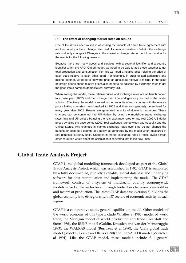
D E C O N O M I C M O D E L S U S E D T O A N A L Y S E T H E T R A D E
79
D.2 The effect of changing market rates on results
One of the issues often raised in assessing the impacts of a free trade agreement with another country is the exchange rate used. A common question is ‘what if the exchange rate suddenly changes’? Changes in the market exchange rate turn out to not matter for the results for the following reasons.
Because there are many goods and services with a sectoral identifier and a country identifier within the APG–Cubed model, we need to be able to add these together to get total production and consumption. For this we need a relative price relating the price of each good relative to each other good. For example, in order to add agriculture and mining together, we need to know the price of agriculture relative to mining. In the case of foreign goods, these relative prices also need to be adjusted by exchange rates to get the good into a common domestic real currency unit.
When solving the model, these relative prices and exchange rates are all benchmarked to a base year (2002) and then change over time endogenously as part of the model solution. Effectively the model is solved in the real units of each country with the relative prices linking countries, benchmarked to 2002 and then endogenously determined for every year after 2002. Results are generated in units of domestic resources. These changes can be converted into US dollars by using the model-generated exchange rates, into real US dollars by using the real exchange rates or into real 2002 US dollar prices by using the base period (2002) real exchange rate between say Australia and the United States. Any changes in market exchange rates over time do not change the benefits or costs to a country of a policy as generated by the model when measured in real domestic currency units. Changes in market exchange rates or price levels across other countries would affect the calculation if converted into those new units.
Global Trade Analysis Project GTAP is the global modelling framework developed as part of the Global Trade Analysis Project, which was established in 1992. GTAP is supported by a fully documented, publicly available, global database and underlying software for data manipulation and implementing the model. The GTAP framework consists of a system of multisector country economywide models linked at the sector level through trade flows between commodities and factors of production. The latest GTAP database (version 5) divides the global economy into 66 regions, with 57 sectors of economic activity in each region.
GTAP is a comparative static, general equilibrium model. Other models of the world economy of this type include Whalley’s (1985) model of world trade, the Michigan model of world production and trade (Deardoff and Stern 1986), the RUNS model (Goldin, Knusden and van der Mensbrugghe 1993), the WALRAS model (Burniaux et al 1990), the CIE’s global trade model (Stoeckel, Pearce and Banks 1990) and the SALTER model (Zeitsch et al 1991). Like the GTAP model, these models include full general
M E A S U R I N G T H E P O S S I B L E I M P A C T S O F M A F T A
80
D E C O N O M I C M O D E L S U S E D T O A N A L Y S E T H E T R A D E
equilibrium features of individual economies and link these economies through international trade. Some (for example, the latest version of SALTER) also have linkages through international capital markets.
In the GTAP model the activities of economic agents — consumers, produc-ers and government — are modelled according to neoclassical economic theory. Consumers are assumed to maximise utility and producers to maxi-mise profits. Markets are assumed to be perfectly competitive. Production exhibits constant returns to scale. Different regions and economies are link-ed through trade. Some of these assumptions — for example, constant returns to scale — mean that the gains from trade liberalisation will typically be understated by GTAP.
The change in welfare reported by the GTAP model arises principally from the reallocation of resources within an economy and the resulting change in allocative efficiency. Welfare may also change as a result of terms of trade effects, which may be significant for some countries. GTAP does not permit any statement about the time path of benefits and capital flows that allow consumers to borrow and so vary their real consumption patterns over time. Important dynamic gains from trade liberalisation are not captured in a comparative static model of this kind.
Accounting for investment flows in the standard GTAP model
The standard GTAP framework allows users to specify whether the global allocation of investment is fixed or flexible. The former view assumes that the regional composition of capital stocks does not change in response to the policy change, meaning that global and regional net investment move together. As shown by the accounting identity C.1, provided there is little change in regional savings, fixing the global bank’s allocation of investment effectively fixes the trade balance (capital account) for each country/region.
S I X M R− ≡ − + C.1
Identity C.1 states that national savings (S) minus investment (I) is equivalent to the current account, where R is international transfer receipts (which are set to zero in the GTAP database) (Hertel 1997).
Alternatively, the allocation of investment across regions can be made flexible, driven by the (expected) rate of return to capital. Investors are assumed to behave in such as to equate the rate of return across regions. Investment flows to/from a region depend on that region’s rate of return to capital relative to the rate prevailing elsewhere. By identity C.1, an increase
M E A S U R I N G T H E P O S S I B L E I M P A C T S O F M A F T A

D E C O N O M I C M O D E L S U S E D T O A N A L Y S E T H E T R A D E
81
in regional investment would be associated with a deterioration in the current account and a strengthening of the terms of trade.
Investment in the standard GTAP model does not come on-line in the simulation period, meaning that the capital stock within an economy is fixed. This outcome is essentially a short run proposition — the simulation period is too short to allow any investment that may affect the stock of capital. GTAP’s investment theory does not allow it to be used for true long-run policy analysis (Hanslow et al 2000 p.21).
Plainly, the GTAP model has some limitations for longer-run applications because it does not account for capital and wealth accumulation. The APG–Cubed model, which is better equipped than GTAP to incorporate and model changes to financial and capital flows, is better placed to investigate the effects of a trade agreement between Australia and Malaysia on capital flows and accumulation, and has been employed for that purpose in this study. But it was also used to calibrate the GTAP investment function and allow accumulation relationships to be approximated in GTAP. These developments are described in the next section.
Modifying the standard GTAP model: Investment, Savings and Asset Accumulation
The standard GTAP model has been modified to better accommodate the impacts of the FTA on the financial and real sectors.
When the standard GTAP model is used with the flexible investment specification the responsiveness of investment is governed by a user-specified parameter that is called RORFLEX (standing for ‘rate of return flexibility’).4 The value of RORFLEX was chosen so that, for a particular simulation, GTAP produced the same investment response as APG–Cubed after about 10 years. The simulation used for this purpose was the removal, by both Australia and Malaysia, of import tariffs on merchandise goods.
The APG–Cubed simulation was further used to quantify how the change in a country’s capital stock is linked to the magnitude of the policy-induced change in investment after about 10 years. In the APG–Cubed simulation a policy-induced change in investment that was 1 per cent higher than the baseline after a decade caused about a 0.34 per cent change in the capital
4 The sensitivity of model results with respect to this parameter is assessed in
chapter 7.
M E A S U R I N G T H E P O S S I B L E I M P A C T S O F M A F T A

82
D E C O N O M I C M O D E L S U S E D T O A N A L Y S E T H E T R A D E
stock in Australia after 10 years.5 GTAP was modified to make the capital stock responsive to investment with an elasticity of 0.34.
The changes to GTAP described so far would lead to an overstatement of the benefits of any policy that was advantageous to investment. The income accounting in GTAP assumes that all income from capital located in a particular country accrues to that country. This may be satisfactory when GTAP is used as a purely comparative static model, but once accumulation effects are introduced the issue of who finances an expansion in the capital stock, and to whom the returns accrue, must be addressed. So GTAP was modified to include a relationship between the savings of a country and its accumulation of wealth.6 The elasticity of wealth with respect to savings was set at a value of 0.33.7 The difference between capital located in a country and the wealth of the country is the net foreign assets of the country from which income is earned (or upon which interest must be paid if net foreign assets are negative).
Other modifications to the standard GTAP model
The default closure of the standard GTAP model has aggregate employ-ment fixed. By contrast, APG–Cubed allows both real wages and aggregate employment to adjust to a policy change, with employment eventually returning to its baseline level. However, as can be observed from APG–Cubed simulations, the deviation of employment from its baseline levels can persist for many years. As described in the previous section, the invest–ment and accumulation behaviour of GTAP has been calibrated to a time frame of about 10 years. Therefore, it is consistent to calibrate GTAP’s labour market behaviour to a similar time frame. APG–Cubed results, for the same simulation used to calibrate investment and accumulation behaviour, provide a ten-year-out relationship between real wages and employment of the form:
l=0.46*w C.2
where l is the percentage deviation in aggregate employment from its baseline level, and w is the deviation in the real wage from its baseline level. The inclusion of this relationship in GTAP means that the effects of
5 The value of 0.34 is within the range of values 0.3-0.4 found and used in previous
studies by the CIE (2004). 6 Wealth in this context is the capital owned by a country. 7 This is slightly lower than the elasticity of capital with respect to investment as
saving is less than investment for New Zealand.
M E A S U R I N G T H E P O S S I B L E I M P A C T S O F M A F T A

D E C O N O M I C M O D E L S U S E D T O A N A L Y S E T H E T R A D E
83
any policy on the labour market are partitioned between a change in the real wage and a change in aggregate employment.
The GTAP database
Input-output data and trade data
As the GTAP model will be used for the detailed sectoral results, it is important that the underlying database is as up-to-date as possible. Version 5 of the GTAP database — the latest available — is based on 1997 data. However, since 1997 changes will have occurred to the structure, size and trade patterns of various economies within the model. To improve the accuracy of the country and sector detailed results it is important that the database be updated to reflect changes that have occurred since 1997 (Version 6 of the database, pertaining to year 2001 and covering 78 regions and 57 sectors of production, with improved services trade data, is expected to be released in Autumn 2005).
Updating the database has been achieved by using the latest available data to update key components of the database. These include:
macroeconomic aggregates (GDP, domestic absorption, exports and imports); and
trade flows and trade distortions.
A critical outcome of the updating procedure is that relativities between the GDPs of Australia, Malaysia and their major trading partners such as New Zealand, the United States, Japan and ASEAN members are correct. Data for macro aggregates was obtained from the World Development Report 2003, for exports and imports between Australia, Malaysia and major trading partners thereof from the World Trade Atlas, and trade distortions from tariff schedules provided by DFAT and knowledge of existing and future free trade agreements between key regions. For example, the Australia–Singapore, Australia–Thailand, and Australia–United States free trade agreements were included in the database.
Updating the entire GTAP bilateral trade database for all countries is a substantial undertaking. Hence in the updating procedure CIE has updated critical bilateral trade flows between Australia, Malaysia and their major trading partners. All other trade flows have been updated according to existing database shares but consistently with macroeconomic data. A modified RAS procedure has been used to adjust the database.
M E A S U R I N G T H E P O S S I B L E I M P A C T S O F M A F T A
84
D E C O N O M I C M O D E L S U S E D T O A N A L Y S E T H E T R A D E
Parameters
The GTAP database also contains values for various elasticities determining:
1. substitution between domestic and imported varieties of each commodity (loosely referred to as the Armington parameters);
2. substitution between primary factors (the default values being chosen to reproduce typical supply elasticities for natural resource using industries);
3. substitution between primary factors as a whole and intermediate inputs (set to zero by default);
4. price and income responsiveness of private consumption demand for each commodity; and
5. responsiveness of investment to rates of return (the parameter called RORFLEX).
The choice of Armington parameters are critical for the results in trade liberalisation studies. The default GTAP values for the Armington parameters were used for all GTAP sectors except Motor Vehicles and Parts for Australian exports to Malaysia. These were reduced to represent the actual substitution between Australian motor vehicle exports that are typically six cylinder cars and the four cylinder cars that dominate the Malaysian passenger motor vehicle market. Although these two products are generally substitutable, a domestic excise tax imposed by the Malaysian Government based on the size of the car’s engine has reduced the substitution between the two products. In particular, passenger motor vehicles that have an engine capacity greater than 2.5 litres face a relatively large excise tax which increases the price for these types of vehicles and therefore favours motor vehicles with smaller engines. Any free trade agreement between Australian and Malaysia would not remove this excise tax. Consequently, even after large reductions of tariff levels in passenger motor vehicles under MAFTA, Australian exporters would still find it difficult to sell into the Malaysian market as they still face a prohibitive excise structure and policies for the domestic industry that favour cars with smaller engines than Australia currently exports (Andrew McKellar, Federal Chamber of Automotive Industries, personal communication, 9 November 2004).
The reduction in Armington elasticities for the Motor Vehicles and Parts sector was calculated by reducing the Armington elasticity for motor vehicles and parts by the portion of passenger motor vehicle sales in Malaysia that have an engine capacity less than 2.5 litres and the portion of
M E A S U R I N G T H E P O S S I B L E I M P A C T S O F M A F T A

D E C O N O M I C M O D E L S U S E D T O A N A L Y S E T H E T R A D E
85
D.3 Mapping between databases — GTAP regions
Aggregated GTAP regions GTAP regions
Australia Australia
China China
European Union (25) Austria, Belgium, Denmark, Finland, France, Germany, Greece, Hungary, Ireland, Italy, Luxembourg, Netherlands, Poland, Portugal, Rest of Central European Associates, Spain, Sweden, United Kingdom
Indonesia Indonesia
Malaysia Malaysia
New Zealand New Zealand
North Asia Japan, Hong Kong, Taiwan, South Korea
Philippines Philippines
Singapore Singapore
Thailand Thailand
United States United States
Vietnam Vietnam
Rest of World Argentina, Bangladesh, Botswana, Brazil, Canada, Central America and the Caribbean, Chile, Colombia, Former Soviet Union, India, Malawi, Mexico, Morocco, Mozambique, Other Southern Africa, Rest of Andean Pact, Peru, Rest of EFTA, ,Rest of Middle East, Rest of North Africa, Rest of South Africa Customs Union, Rest of South America, Rest of South Asia, Rest of Sub Saharan Africa, Sri Lanka, Switzerland, Tanzania, Turkey, Uganda, Uruguay, Venezuela, Zambia, Zimbabwe, Rest of World
Source: CIE.
Australian motor vehicle exports in the Australian motor vehicles and parts sector.
Parameter groups 2-4 were left at their default GTAP values. The choice of RORFLEX based on APG–Cubed results was discussed previously under modifications of the GTAP model.
Aggregating the GTAP database
The GTAP database has considerable regional and commodity detail, encompassing 66 regions and 57 sectors of production. Due to the size of the underlying database, an aggregated version of the database has been used to analyse the economic implications of the FTA (in order to keep the modelling manageable). The 66 regions and 57 sectors have been condensed to 13 regions, while the sectors remain as is (that is, the sectors have not undergone any aggregation). The mapping between the 66 region GTAP database and the aggregated 13 region version of the database used here is shown in table D.3.
Full documentation for the GTAP economic model can be found at www.gtap.agecon.purdue.edu/default.asp.
M E A S U R I N G T H E P O S S I B L E I M P A C T S O F M A F T A

86
References
ABS (Australian Bureau of Statistics) 2004, Overseas Arrivals and Departures, Cat. no.3401.0, August 2004, ABS, Canberra.
Aw, B.A., Chung, S. and Roberts, M.J. 2000, ‘Productivity and Turnover in the Export Market: Micro-level Evidence from the Republic of Korea and Taiwan (China)’, The World Bank Economic Review, 14(1), pp. 65–90.
Brown D., Deardorff A. Fox A. and Stern R. 1995, “Computational Analysis of Goods and Services Liberalization in the Uruguay Round”, in Martin W. and Winters A. The Uruguay Round and the Developing Economies, World Bank Discussion Paper, Washington D.C.
Burniaux, J.M., Delorme, F., Leinert, I. and Martin, J.P. 1990, ‘WALRAS — a multi-sector, multi-country applied general equilibrium model for quantifying the economywide effects of agricultural policies’, in OECD, Modelling the Effects of Agricultural Policies, OECD Economic Studies, no. 13, Paris.
Chand, S. 1999, ‘Trade liberalisation and productivity growth: Time-series evidence from Australian manufacturing’, Economic Record, vol. 75, no. 228, p. 28–35.
—— and Vousden, N. 1996, Trade Liberalisation and Productivity Growth: A Panel Data Study of Australian Manufacturing, mimeo, Australian National University, Canberra.
Chuang, Y-C. and Lin, C-M. 1999, ‘Foreign direct investment, R&D and spillover efficiency: Evidence from Taiwan’s manufacturing firms’, The Journal of Development Studies, vol. 35, no. 4, p. 117–37.
CIE, 2004, Economic analysis of AUSFTA: Impact of the bilateral free trade agreement with the United States, Centre for International Economics
——2004a, Measuring the possible impact of an FTA between New Zealand and China, Centre for International Economics
Deardoff, A.V. and Stern, R.M. 1986, The Michigan Model of World Production and Trade, MIT Press, Cambridge, Massachusetts.
Frankel, J.A. and Romer, D. 1999, ‘Does trade cause growth?’, The American Economic Review, vol. 89, no. 3, pp. 379-99.
M E A S U R I N G T H E P O S S I B L E I M P A C T S O F M A F T A

R E F E R E N C E S
87
Goldin, I, Knudsen, O. and van der Mensburgghe, D. 1993, Trade Liberalisation: Global Economic Implications, OECD and World Bank, Paris.
Hanslow, K., Phamduc, T. and Verikios, G. 2000, The Structure of the FTAP Model, Productivity Commission Research Memorandum no. 58, Canberra.
Hoekman B. 1995, Tentative First Steps: an Assessment of the Uruguay Round Agreement on Services, World Bank Policy Research Paper No. 1455, May.
Holmes L. and Hardin A. 2000, “Assessing Barriers to Services Sector Investment”, in Findlay C. and Warren T., Impediments to Trade in Services: Measurement and Policy Implications, Routledge, New York and London.
Ianchovichina, E., Binkley, J. and Hertel, T. 2000, ‘Procompetitive effects of foreign competition on domestic markups’, Review of International Economics, vol. 8, no. 1, pp. 134–48.
Itakura, K., Hertel, T.W. and Reimer, J.J. 2003, The Contribution of Productivity Linkages to the General Equilibrium Analysis of Free Trade Agreements, GTAP Working Paper 23, March 2003, http://www.gtap.agecon.purdue.edu/ resources/download/1296.pdf, Accessed 22 November 2004.
Kalirajan K., McGuire G., Nguyen-Hong D. and Schuele M. 2000, “The Price Impact of Restrictions on Banking Services”, in Findlay C. and Warren T. (eds), op. cit.
MacDonald, J.M. 1994, ‘Does import competition force efficient production?’ Review of Economics and Statistics, vol. 76, no. 4, pp. 721–7
McGuire G. and Schuele M. 2000, “Restrictiveness of International Trade in Banking Services”, in Findlay C. and Warren T.(eds), op. cit.
McKibbin, W. 1996, Quantifying APEC Trade Liberalisation: A Dynamic Analysis, Working Paper in Trade and Development no. 1, Economics Department, Research School of Pacific and Asian Studies, Australian National University, Canberra, and Brookings Discussion Paper in International Economics no. 122, Brookings Institution, Washington, DC.
—— and Sachs, J.D. 1991, Global Linkages: Macroeconomic Interdependence and Cooperation in the World Economy, Brookings Institution, Washington, DC.
Nguyen-Hong D. 2000, Restrictions on Trade in Professional Services, Productivity Commission Staff Research Paper, AusInfo, Canberra, August.
Nguyen-Hong D. and Wells R. 2003, Restrictions on Trade in Education Services: Some Basic Indexes, Productivity Commission Staff Working Paper, Canberra, October.
Stoeckel, A., Pearce, P. and Banks, G. 1990, Western Trade Blocs: Game, Set or Match for Asia-Pacific and the World Economy?, Confederation of Asia-Pacific Chambers of Commerce and Industry, Canberra.
M E A S U R I N G T H E P O S S I B L E I M P A C T S O F M A F T A

88
R E F E R E N C E S
Tourism Australia 2004a, Malaysia Market Snapshot, http://www. tourism.australia.com/content/Malaysia/2004_profiles/market_snapshot_malaysia.pdf, published July 2004, Accessed 14 October 2004.
——2004b, Malaysia Visitor Analysis, http://www.tourism.australia.com/ content/Malaysia/2004_profiles/visitor_analysis_malaysia.pdf, published October 2004, Accessed 14 October 2004.
OECD (Organisation for Economic Cooperation and Development) 1997, Measure-ment of Non-Tariff Barriers, Economics Department Working Papers, no.179, http://www.oecd.org/dataoecd/34/3/1863859.pdf, Accessed 6 July 2004.
Roberts, P. 2004,’Life on the open market’, in The Australian Financial Review, 19 October 2004, pp. 1 and 60.
Rodriguez, F. and Rodrik, D. 1999, Trade policy and economic growth: A skeptic’s guide to the cross national evidence, NBER, Working paper 7081, April
UK Trade and Investment, 2004, Financial services industry in Malaysia, www.trade.uktradeinvest.gov.uk/financial/malaysia/profile/overview.shtml, accessed 01 November, 2004
USTR (United States Trade Representative) 2004, 2004 National Trade Estimate on Foreign Barriers to Trade, http://www.ustr.gov/reports/nte/2004/fulltext.pdf, Accessed 5 July 2004.
Wacziarg, R. 2001, ‘Measuring the dynamic gains from trade’, The World Bank Economic Review, vol. 15, no. 3, pp. 393-429.
Whalley, J. 1985, Trade Liberalization Among Major Trading Areas, MIT Press, Cambridge, Massachusetts.
WB (World Bank) 2002, Global Economic Prospects and the Developing Countries.
Zeitsch, J., McDougall, R., Jomini, P., Welsh, A., Hambley, J., Brown, S. and Kelly, J. 1991, SALTER: A General Equilibrium Model of the World Economy, SALTER Working Paper no. 4, Industry Commission, Canberra.
M E A S U R I N G T H E P O S S I B L E I M P A C T S O F M A F T A