Measuring the overhead of Intel C++ Concurrent … the overhead of Intel C++ Concurrent Collections over Threading Building Blocks for Gauss–Jordan ... the ease of programming and

CONCURRENCY AND COMPUTATION: PRACTICE AND EXPERIENCEConcurrency Computat.: Pract. Exper. 2012; 24:2282–2301Published online 26 January 2012 in Wiley Online Library (wileyonlinelibrary.com). DOI: 10.1002/cpe.2811

Measuring the overhead of Intel C++ Concurrent Collections overThreading Building Blocks for Gauss–Jordan elimination

Peiyi Tang*,†

Department of Computer Science, University of Arkansas at Little Rock, Little Rock, AR 72204, USA

SUMMARY

The most efficient way to parallelize computation is to build and evaluate the task graph constrained onlyby the data dependencies between the tasks. Both Intel’s C++ Concurrent Collections (CnC) and ThreadingBuilding Blocks (TBB) libraries allow such task-based parallel programming. CnC also adapts the macrodata flow model by providing only single-assignment data objects in its global data space. Although CnCmakes parallel programming easier, by specifying data flow dependencies only through single-assignmentdata objects, its macro data flow model incurs overhead. Intel’s C++ CnC library is implemented on top ofits C++ TBB library. We can measure the overhead of CnC by comparing its performance with that of TBB.In this paper, we analyze all three types of data dependencies in the tiled in-place Gauss–Jordan elimina-tion algorithm for the first time. We implement the task-based parallel tiled Gauss–Jordan algorithm in TBBusing the data dependencies analyzed and compare its performance with that of the CnC implementation. Wefind that the overhead of CnC over TBB is only 12%–15% of the TBB time, and CnC can deliver as muchas 87%–89% of the TBB performance for Gauss–Jordan elimination, using the optimal tile size. Copyright© 2012 John Wiley & Sons, Ltd.

Received 23 August 2011; Revised 11 December 2011; Accepted 11 December 2011

KEY WORDS: task-based parallel execution; graph-driven asynchronous execution; Intel C++ CnC; IntelC++ TBB; data dependency analysis; tiled Gauss–Jordan elimination

1. INTRODUCTION

Coarse-grain loop-based parallel software packages such as LAPACK [1] have shown limitations onemerging multicore architectures [2] because of the large granularity of computation and the overspecification inherited in the loop-based fork-join paradigm. The most efficient approach of parallelexecution is to build and evaluate the task graph constrained only by the data dependencies betweenthe tasks without over specification [3]. Fine-grain tasks can also fit the data accessed into the smallcaches of the cores.Both Intel’s C++ Concurrent Collections (CnC) [4] and Threading Building Blocks (TBB) [5, 6]

libraries allow such task-based parallel programming. CnC also adapts the macro data flow model[7] by allowing only single-assignment data objects in its Linda-tuple-space-like [8] global spacecalled CnC context. Each computational task in CnC is purely functional and side-effect free. There-fore, only flow data dependencies between the tasks need to be honored, and they can be enforcedthrough the single-assignment data objects in the CnC context. This makes parallel programming inCnC much easier [9, 10].Intel’s C++ CnC library for shared-memory multicore processors is implemented on top of

Intel’s TBB library [5, 6] for task-based asynchronous multicore parallel programming. TBB isnot functional, and tasks in TBB read and write the shared memory of multicore computers directly.

*Correspondence to: Peiyi Tang, Department of Computer Science, University of Arkansas at Little Rock, Little Rock,AR 72204, USA.†E-mail: [email protected]

Copyright © 2012 John Wiley & Sons, Ltd.

MEASURING THE OVERHEAD OF INTEL C++ CnC OVER TBB FOR GAUSS–JORDAN ELIMINATION 2283

Implementing the data flow model on shared memory incurs overhead because the data objectsneeded by tasks need to be copied from the context. The data produced by tasks also need to becopied to the context. The associative search with tags for data and task objects in the context alsoincurs overheads.In principle, every task-based asynchronous parallel computation (also known as graph-driven

asynchronous execution) can be specified and executed in both CnC and TBB. The trade-off betweenthe ease of programming and the efficiency of the program has always been a major factor indetermining whether or not to adapt a new programming model or language. We are interested inquantifying the overhead of CnC over TBB. In this paper, we use the tiled Gauss–Jordan eliminationalgorithm for inverting matrices to measure the overhead of CnC over TBB.The Gauss–Jordan elimination algorithm is one of the several dense linear algebra algorithms

used in many scientific applications especially those involving optimization and visualization. It hasO.n3/ time complexity using O.n2/ data space. The tiled Gauss–Jordan algorithm uses a blockarray layout [11] for better cache performance, and the computations on array tiles (blocks) fit thetask-based parallel model of CnC and TBB well. The past parallel tiled Gauss–Jordan algorithmseither explore only the loop-based parallelism [12] or are restricted on the augmented system usingtwo data arrays [13].In this paper, we analyze and formulate all the data dependencies between the tasks in the tiled

in-place Gauss–Jordan algorithm for the first time and parallelize and implement the algorithmin TBB.We compare the TBB performance with the performance of the CnC implementation [4]. We find

that the overhead of CnC over TBB on Gauss–Jordan elimination is only 12%–15% of the TBB timefor the CnC with tuner and 18%–22% of the TBB time for the CnC without tuner, using the optimaltile size. Given that giga floating-point operations per second (GFLOPS) performance is propor-tional to the reciprocal of execution time, CnC with and without tuner can thus deliver as muchas 87%–89% and 82%–85% of the TBB GFLOPS performance, respectively, using the optimaltile size.The rest of the paper is organized as follows. Section 2 presents the data dependency

analysis of all three kinds of dependencies (flow, anti, and output) of the tiled in-placeGauss–Jordan algorithm. Section 3 introduces the CnC model and an implementation of the paral-lel tiled Gauss–Jordan algorithm in CnC. Section 4 describes the implementation of the task-basedparallel tiled Gauss–Jordan algorithm in TBB using the data dependencies analyzed and formulatedin Section 2. Section 5 presents our experimental results of both CnC and TBB parallel codes, aswell as the sequential tiled code, analyzes their performances, and finds the overhead of CnC overTBB. Section 6 describes work related to ours and future work. Section 7 concludes the paper witha discussion.

2. PARALLELIZING TILED IN-PLACE GAUSS–JORDAN ELIMINATION

Gauss–Jordan elimination is an algorithm to invert a matrix A to A�1. The sequential tiled Gauss–Jordan elimination parallelized in [12,13] inverts A with an identity matrix B and has A�1 stored inB when the algorithm is finished. A modified in-place algorithm that inverts A in place and storesA�1 in A is shown in Figure 1. The in-place algorithm reduces the number of matrix data arraysused from two to one and the number of task types from six to four. In Figure 1, an n � n matrixdata array is tiled to a d � d tile array. Each tile is a t � t data array with t D n=d denoted as Aij

(0 6 i , j 6 d � 1). The k-th (k D �1, 0, � � � , d � 1/ version of the tile Aij is denoted as A.k/ij in the

algorithm of Figure 1. A.k/ij can also be regarded as the k-th value stored in Aij . The initial value of

Aij can be seen as A.�1/ij . The initial matrix is the collection of A

.�1/ij (0 6 i , j 6 d � 1), and the

final inverted matrix is the collection of A.d�1/ij (0 6 i , j 6 d � 1).

As can be seen from Figure 1, in each iteration of the outermost loop k, each tile Aij (0 6 i , j 6d � 1) is updated once, by one of the four types of computation as shown in Table I. Thus, thecomputation of updating tile Aij in the k-th (k D 0, � � � , d � 1) iteration of the outermost loop canbe regarded as task .k, i , j /. The tasks with the same index k are called the tasks of iteration k.

Copyright © 2012 John Wiley & Sons, Ltd. Concurrency Computat.: Pract. Exper. 2012; 24:2282–2301DOI: 10.1002/cpe

2284 P. TANG

Figure 1. Tiled in-place Gauss–Jordan elimination algorithm.

There are total of d 3 tasks with indexes .k, i , j / (0 6 k, i , j 6 d � 1). The quantity column ofTable I shows the total number of tasks of the type. Table I also shows the number of floating-pointoperations in each type of task.‡ Recall that d D n=t . The total number of floating-point operationsas a function of problem size n and tile size t , denoted as flop(n,t), is as follows

flop.n, t / D�

1

tC 2

�n3 � 2n2 � .t � 1/n. (1)

It can also be expressed as a function of problem size n and tile array dimension d , denoted asflop(n,d), as follows

flop.n, d/ D 2n3 C��

d � 1

d

�� 2

�n2 C n. (2)

The partial derivative of flop.n, d/ with respect to d is @flop.n,d/@d

D n2.1 C 1d2 / > 0. Thus,

flop.n, d/ is an increasing function of d and thus, flop.n, t / is a decreasing function of t . When t

changes from 1 to n, flop.n, t / decreases from 3n3 � 2n2 to 2n3 � 2n2 C n.The most efficient parallel execution of dense linear algebra algorithms on multicore processors is

to build the task graph of the data dependencies among the tasks and execute the tasks of the graphby honoring these dependencies [14, 15]. There are three kinds of data dependencies: flow (RAW,read after write), anti (WAR, write after read), and output (WAW, write after write) data dependen-cies. Task B is flow/anti dependent on task A, denoted as A ! B/A 7! B , if it reads/writes thedata written/read by task A earlier. Task B is output-dependent on task A if it writes the data writtenby task A earlier. Flow data dependencies are the essential ones and must be honored in any par-allel programming model. Anti and output data dependencies can be eliminated by renaming dataobjects as in the single-assignment programming models, such as CnC or functional programming

Table I. Type, computation, and number of flops of task .k, i , j /.

Type Condition Quantity Computation No. of flops

I i D k ^ j D k d A.k/kk

D .A.k�1/kk

/�1 2t3 � 2t2 C t

IIj i D k ^ j ¤ k d.d � 1/ A.k/kj

D A.k/kk

A.k�1/kj

2t3

IIi i ¤ k ^ j D k d.d � 1/ A.k/ik

D �A.k�1/ik

A.k/kk

2t3

III i ¤ k ^ j ¤ k d.d � 1/2 A.k/ij D A

.k�1/ij � A

.k�1/ik

A.k/kj

2t3 C t2

‡The floating-point operations include addition, subtraction, multiplication, and division between two floating-pointnumbers.



languages. For the shared memory models such as TBB, the task graph has to include all the flow,anti, and output data dependencies.The loop-based approach to parallelize the algorithm in Figure 1 would keep the outermost loop

k serial and find parallelism in its loop body based on the data dependency analysis between thetask types of the same iteration k. Figure 2 shows the flow and anti dependencies between differenttypes of tasks of the same iteration k. Because type IIj and type IIi tasks read tile Akk writtenby the type I task, type IIj and IIi tasks are flow dependent on the type I task. As type III tasksread tiles Akj , written by the corresponding (with the same j index) type IIj tasks, type III tasksare flow dependent on type IIj tasks (with the same j index). These flow data dependencies areshown by the solid arrows in Figure 2. Because type IIi tasks write the tiles Aik that are read by thecorresponding type III tasks (with the same index i) earlier, there is an anti dependency from thetype III tasks to the corresponding type IIi tasks, shown by the dashed arrow in Figure 2. There areno output dependencies between the tasks of the same iteration k because every tile is written onlyonce by one of these tasks.Note that type IIi tasks do not read the tiles Aij written by type III tasks, and they are the only

tasks in the current iteration k that execute after type III tasks. Therefore, there are no tasks in thecurrent iteration k that read the data written by type III tasks. There are also no tasks in the currentiteration k that read the data written by type IIi tasks because type IIi tasks are the last ones inthe iteration.As long as the flow and anti data dependencies between the task types shown in Figure 2 are hon-

ored, the tasks of the same type can be executed in parallel because there are no data dependenciesamong them. The loop-based parallel Gauss–Jordan elimination, based on the dependency graph inFigure 2, would be as shown in Figure 3. The parallel execution of the tasks of the same type is spec-ified by the parallel forall loops§ in Figure 3, and the flow and anti data dependencies betweentask types are honored by the sequential order of these parallel loops. Note that a parallel loop can-not start its iterations unless all the iterations of the preceding parallel loop are completed. It is thisfork-join synchronization of the parallel loop semantics that enforces all the data dependencies inFigure 2.However, as shown by previous studies [14–16], the performance of loop-based algorithms is

always inferior to that of task-based algorithms, partly because of the over specification of this fork-join synchronization. Another reason is that loop-based algorithms cannot explore the parallelism

Figure 2. Data dependency graph of task types in the same iteration k.

§The nested parallel forall loops are two-dimensional parallel loop, and all the tasks of type III enclosed can beexecuted in parallel.


2286 P. TANG

Figure 3. Loop-based parallel Gauss–Jordan elimination algorithm.

between the tasks in different iterations of the outermost loop k, as it cannot be parallel because ofits cross-iteration dependencies.The dependency graph in Figure 2 cannot be used for task-based parallelization. What we need

for task-based parallel execution is a dependency graph between all the individual tasks in the entirealgorithm. In the following, we analyze and formulate the flow, anti, and output data dependenciesamong all the tasks.

2.1. Flow data dependency

Because every tile Aij (0 6 i , j 6 d � 1) is updated (written) in every iteration of loop k, thetasks that a task in iteration k is flow dependent on are either in the same iteration k or the previousiteration k � 1. In particular, task .k, i , j / of all types always reads tile Aij , which is written bytask .k � 1, i , j / (if k > 0), and thus, task .k, i , j / is flow dependent on task .k � 1, i , j /. This issummarized as Lemma flow-0 in Table II, which says that if k > 0, then f.k � 1, i , j /g ! .k, i , j /.Notation P ! .k, i , j / means p ! .k, i , j / for every p 2 P , and P is called a predecessor set oftask .k, i , j /. In addition, type IIj task .k, k, j / with j ¤ k reads tile Akk written by task .k, k, k/.Thus, task .k, k, j / with j ¤ k is flow dependent on task .k, k, k/. This is summarized as Lemmaflow-2.1 in Table II. Similarly, type IIi task .k, i , k/ with i ¤ k is flow dependent on task .k, k, k/

as summarized as Lemma flow-2.2 in Table II. Type III task .k, i , j / with i ¤ k and j ¤ k readsvalues A

.k�1/

ikand A

.k/

kjfrom tiles Aik and Akj written by tasks .k � 1, i , k/ (if k > 0) and .k, k, j /,

respectively. Thus, task .k, i , j / is flow dependent on tasks .k �1, i , k/ (if k > 0) and .k, k, j /. Thisis summarized as Lemmas flow-3.1 and flow-3.2, respectively, in Table II.Note that the predecessors shown by Lemma flow-0 and flow-3.2 are from the previous iteration

of loop k. The remaining predecessor sets are from the current iteration of loop k.From the flow dependency predecessors of task .k, i , j / in Table II, the flow dependency succes-

sors for task .k, i , j / can be derived. Table III shows the Lemmas for the set of successors of alltypes of tasks. Lemma flow-D0 is the duel of Lemma flow-0 shown in Table II. Likewise, Lemmaflow-D2.1-2 is the duel of Lemma flow-2.1 and flow-2.2. Lemmas flow-D3.1 and flow-D3.2 are theduals of Lemmas flow-3.1 and flow-3.2, respectively.

Table II. Flow dependency predecessors of task .k, i , j /.

Lemma Type Condition Set of processors

flow-0 All k > 0 f.k � 1, i , j /g ! .k, i , j /flow-2.1 IIj i D k ^ j ¤ k f.k, i , k/g ! .k, i , j /flow-2.2 IIi i ¤ k ^ j D k f.k, k, j /g ! .k, i , j /flow-3.1 III i ¤ k ^ j ¤ k f.k, k, j /g ! .k, i , j /flow-3.2 III i ¤ k ^ j ¤ k ^ k > 0 f.k � 1, i , k/g ! .k, i , j /



Table III. Flow dependency successors of task .k, i , j /.

Lemma Type Condition Set of successors

flow-D0 All k < d � 1 .k, i , j / ! f.k C 1, i , j /gflow-D2.1-2 I i D k ^ j D k .k, i , j / ! f.k, i ,y/ j y ¤ kg[

f.k, x, j / j x ¤ kgflow-D3.1 IIj i D k ^ j ¤ k .k, i , j / ! f.k, x, j / j x ¤ kgflow-D3.2 IIi i ¤ k C 1 ^ j D k C 1 ^ k < d � 1 .k, i , j / ! f.k C 1, i ,y/ j y ¤ k C 1g

Figure 4(a) shows the flow dependencies in the task graph of the tiled Gauss–Jordan eliminationwith 3 � 3 tiles. Each dot is a task of the 3 � 3 � 3 task graph, and arrows are the flow dependenciesbetween the tasks according to Table II or III.

2.2. Anti data dependency

The tasks that a task .k, i , j / is anti dependent on are either of the same iteration k or the previousiteration k � 1. To find the tasks that task .k, i , j / is anti dependent on, we need to check all theprior tasks that reads Aij , ever since task .k � 1, i , j / wrote Aij with value A

.k�1/ij .

For the type I task .k, k, k/, the previous task writing Akk is task .k � 1, k, k/ with value A.k�1/

kk.

Task .k�1, k, k/ is of type III, and no tasks in iteration k�1 read theAkk written by task .k�1, k, k/.Also, type I task .k, k, k/ is the first task in iteration k, and thus, there are no prior tasks in iteration k

to read Akk . Therefore, we can conclude that type I task .k, k, k/ is not anti dependent on any tasks.For a type IIi task .k, i , k/ with i ¤ k, the type III tasks in f.k, i ,y/ j y ¤ kg of the current

iteration k read Aik before the task .k, i , k/ writes it. Thus, we can say that task .k, i , k/ is antidependent on the tasks in f.k, i ,y/ j y ¤ kg or f.k, i ,y/ j y ¤ kg 7! .k, i , k/. This is summarized

k=2

i=0

i=1

i=2

j=1 j=2

i=0

i=0i=1

i=1

i=2

i=2

j=2j=1

j=2j=1

j=0

j=0

j=0

k=0

k=1

(a) Flow Dependencies of 3 × 3 × 3 Task Graph

(b) Anti Dependencies of 3 × 3 × 3 Task Graph

i=1k=0

k=1

k=2

i=0

i=1

i=2

j=0 j=1 j=2

i=0

i=0i=1

i=2

i=2

j=0j=1 j=2

j=2j=0 j=1

Figure 4. (a) Flow and (b) anti dependencies of 3 � 3 � 3 task graph.


2288 P. TANG

as Lemma anti-2.1 in Table IV. To find the tasks of the previous iteration k � 1 that read Aik , wefirst need to remember that Aik was written previously by task .k � 1, i , k/ with value A

.k�1/

ik. If

i ¤ k � 1, task .k � 1, i , k/ is of type III. Thus, no tasks in iteration k � 1 read the values A.k�1/

ikfrom Aij . However, if i D k �1, task .k �1, k �1, k/ is of type IIj . Aik is read by the type III tasksin f.k � 1, x, k/ j x ¤ k � 1g. Thus, f.k � 1, x, k/ j x ¤ k � 1g is a predecessor set of task .k, i , k/

with i D k � 1. This is summarized as Lemma anti-2.2 in Table IV.For a type IIj task .k, k, j / with j ¤ k writing Akj , there are obviously no tasks in the current

iteration k reading value A.k�1/

kjfrom Akj except itself. To find possible tasks in iteration k � 1 that

may read value A.k�1/

kjfrom Akj , which is written by task .k � 1, k, j /, we consider the case of

j ¤ k � 1 first. The task .k � 1, k, j / is of type III because j ¤ k � 1, and thus, there are no tasksin iteration k � 1 reading value A

.k�1/

kjfrom Akj . If j D k � 1, then task .k � 1, k, j / is of type IIi ,

and there are no tasks in iteration k � 1 reading value A.k�1/

kjfrom Akj either. Therefore, type IIj

task .k, k, j / with j ¤ k is not anti dependent on any tasks.For a type III task .k, i , j /with i ¤ k^j ¤ k, there are obviously no tasks in the current iteration

k reading value A.k�1/ij from Aij except itself. To find possible tasks in iteration k �1 that may read

value A.k�1/ij from Aij , which is written by task .k � 1, i , j /, we need to consider the following

four cases:

1. i ¤ k � 1 ^ j ¤ k � 1. In this case, task .k � 1, i , j / writing value A.k�1/ij to Aij is of type III,

and no tasks in iteration k � 1 read A.k�1/ij from Aij .

2. i ¤ k � 1 ^ j D k � 1. In this case, task .k � 1, i , j / is of type IIi , and no tasks in iterationk � 1 read A

.k�1/ij from Aij either.

3. i D k � 1 ^ j ¤ k � 1. In this case, task .k � 1, i , j / is of type IIj , and the type III

tasks in f.k � 1, x, j / j x ¤ k � 1g read A.k�1/ij from Aij . Therefore, task .k, i , j / with

i D k�1^j ¤ k^j ¤ k�1^k > 0 is anti dependent on the tasks in f.k�1, x, j / j x ¤ k�1g.This is summarized as Lemma anti-3.1 in Table IV.

4. i D k � 1 ^ j D k � 1. In this case, task .k � 1, i , j / is of type I, and the type IIi tasks inf.k�1, x, j / j x ¤ k�1g and the type IIj tasks in f.k�1, i ,y/ j y ¤ k�1g read value A

.k�1/ij

from Aij written by task .k � 1, i , j /. Thus, task .k, i , j / with i D k � 1 ^ j D k � 1 ^ k > 0

is anti dependent on the tasks in f.k � 1, x, j / j x ¤ k � 1g and f.k � 1, i ,y/ j y ¤ k � 1g.This is summarized as Lemma anti-3.2 in Table IV.

Similar to flow data dependency, anti data dependency successors of each task can be derived fromthe predecessors in Table IV. The Lemmas for anti data dependency successors of task .k, i , j / areshown in Table V. Lemmas anti-D2.1, anti-D2.2, anti-D3.1, and anti-D3.2 in Table V are the duelsof Lemmas anti-2.1, anti-2.2, anti-3.1, and anti-3.2 in Table IV, respectively.The anti data dependencies of the 3�3�3 task graph for the same tiled Gauss–Jordan elimination

with 3 � 3 tiles, according to Table IV or V, are shown in Figure 4(b) as dashed arrows.

Table IV. Anti dependency predecessors of task .k, i , j /.

Lemma Type Condition Set of processors

anti-2.1 IIi i ¤ k ^ j D k f.k, i ,y/ j y ¤ kg 7! .k, i , j /anti-2.2 IIi i D k � 1 ^ j D k ^ k > 0 f.k � 1, x, j / j x ¤ k � 1g 7! .k, i , j /anti-3.1 III i D k � 1 ^ j ¤ k ^ j ¤ k � 1 ^ k > 0 f.k � 1, x, j / j x ¤ k � 1g 7! .k, i , j /anti-3.2 III i D k � 1 ^ j D k � 1 ^ k > 0 f.k � 1, x, j / j x ¤ k � 1g[

f.k � 1, i ,y/ j y ¤ k � 1g 7! .k, i , j /



Table V. Anti dependency successors of task .k, i , j /.

Lemma Type Condition Set of successors

anti-D2.1 III i ¤ k ^ j ¤ k .k, i , j / 7! f.k, i , k/ganti-D2.2 IIj i ¤ k ^ j D k C 1 ^ k < d � 1 .k, i , j / 7! f.k C 1, k, j /ganti-D3.1 III i ¤ k ^ j ¤ k ^ j ¤ k C 1 ^ k < d � 1 .k, i , j / 7! f.k C 1, k, j /ganti-D3.2 IIi and IIj .i ¤ k ^ j D k _ i D k ^ j ¤ k/ ^ k < d � 1 .k, i , j / 7! f.k C 1, k, k/g

2.3. Output data dependency

In the tiled Gauss–Jordan elimination algorithm, each task .k, i , j / overwrites Aij written by task.k � 1, i , j / (if k > 0). Thus, each task .k, i , j / is only output dependent on task .k � 1, i , j / (ifk > 0). Recall that each task .k, i , j / is also flow dependent on task .k �1, i , j / (if k > 0) as shownby Lemma flow-0 in Table II. Therefore, the output data dependencies are subsumed by the flowdata dependencies, and they need not be enforced.Finally, the task graph of the tiled Gauss–Jordan elimination for shared-memory models is the

graph that consists of all d 3 tasks .k, i , j / (0 6 k, i , j 6 d � 1), with all the flow data dependencyedges determined by Tables II or III and all the anti data dependency edges determined by Tables IVor V. For the 3 � 3 tiled Gauss–Jordan elimination example, the task graph is obtained by includingthe edges in both Figures 4(a) and 4(b).

3. IMPLEMENTATION IN CONCURRENT COLLECTIONS

Concurrent Collections is a novel programming model that separates the specification of computa-tion from that of parallelism. Programmers can define computational steps, data items, and controltags in a CnC context. Each instance of a step or an item has its unique identifier called tag. A stepcollection, the set of instances of a step type, corresponds to exactly one prescribing tag collection,and a step instance can execute only if the matching tag of the tag collection becomes available. Adata collection is the set of instances of a data type that can be assigned only once and cannot beoverwritten. A computation step may produce items and tags. It may also need to input data itemsfrom the CnC context. When tags and data items are produced by a step, they become available. Ifa tag prescribing a step becomes available, the step is prescribed. If all the data items that a stepneeds become available, the step is input-available. A step is enabled if it is both prescribed andinput-available. Only enabled steps may execute. Items and tags may also be input from or outputto the environment, which is the external code invoking the CnC computation. Details of the CnCprogramming model can be found in [4, 9, 10].The implementation of the tiled Gauss–Jordan elimination in CnC described in the succeeding

text is from samples/MatrixInverter/ of the Intel CnC for C++ 0.6 for Linux from [4]. Asanalyzed in Section 2, there are d �d �d tasks .k, i , j / (0 6 k, i , j 6 d �1), updating tile Aij to its

k-th version A.k/ij . In CnC, each data item is a single-assignment object. Therefore, each value A

.k/ij

is stored in a separate data item. Thus, it is natural that we have the following: (i) a step collection forthe tasks .k, i , j / (0 6 k, i , j 6 d �1) to calculate output values A

.k/ij ; (ii) a tag collection of triplets

.k, i , j / (0 6 k, i , j 6 d �1) to prescribe the tasks of the step collection; and (iii) an item collectionof all values A

.k/ij identified by the triplet tag .k, i , j / (0 6 k, i , j 6 d � 1). The initial/final tile

array is input/output from/to the environment as the tiles of version -1/d � 1, that is, A.�1/ij /A.d�1/

ij

(0 6 i , j 6 d � 1). The environment produces all the tags .k, i , j / (0 6 k, i , j 6 d � 1) to pre-scribe all the steps. Because each value A

.k/ij is stored in separate data item, all the anti and output

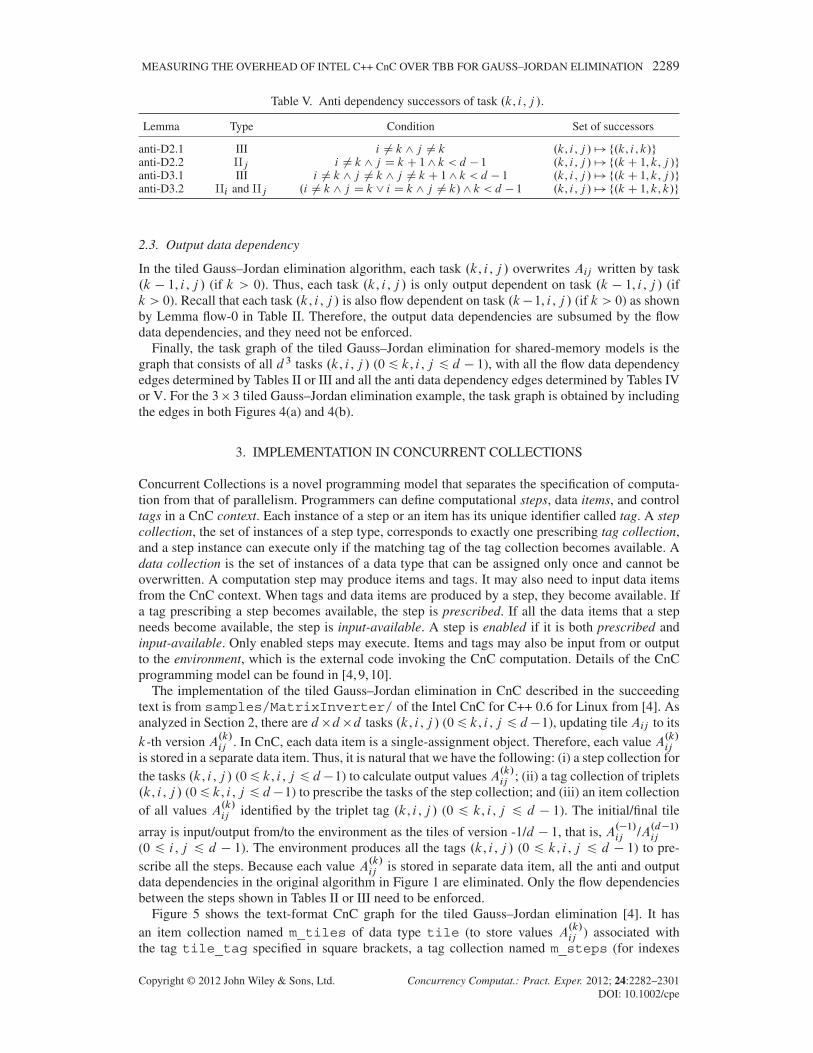
data dependencies in the original algorithm in Figure 1 are eliminated. Only the flow dependenciesbetween the steps shown in Tables II or III need to be enforced.Figure 5 shows the text-format CnC graph for the tiled Gauss–Jordan elimination [4]. It has

an item collection named m_tiles of data type tile (to store values A.k/ij ) associated with

the tag tile_tag specified in square brackets, a tag collection named m_steps (for indexes


2290 P. TANG

Figure 5. Concurrent collection graph for tiled Gauss–Jordan elimination [4].

.k, i , j /) associated with tags tile_tag specified in angle brackets, and a step collection namedcompute_inverse (for tasks) specified in parentheses. The arrow -> shows the producer andconsumer relations between items and steps, and double colon :: shows the relation of prescriptionbetween tags and steps.The producer and consumer relations in the CnC graph in Figure 5 do not show the detail of

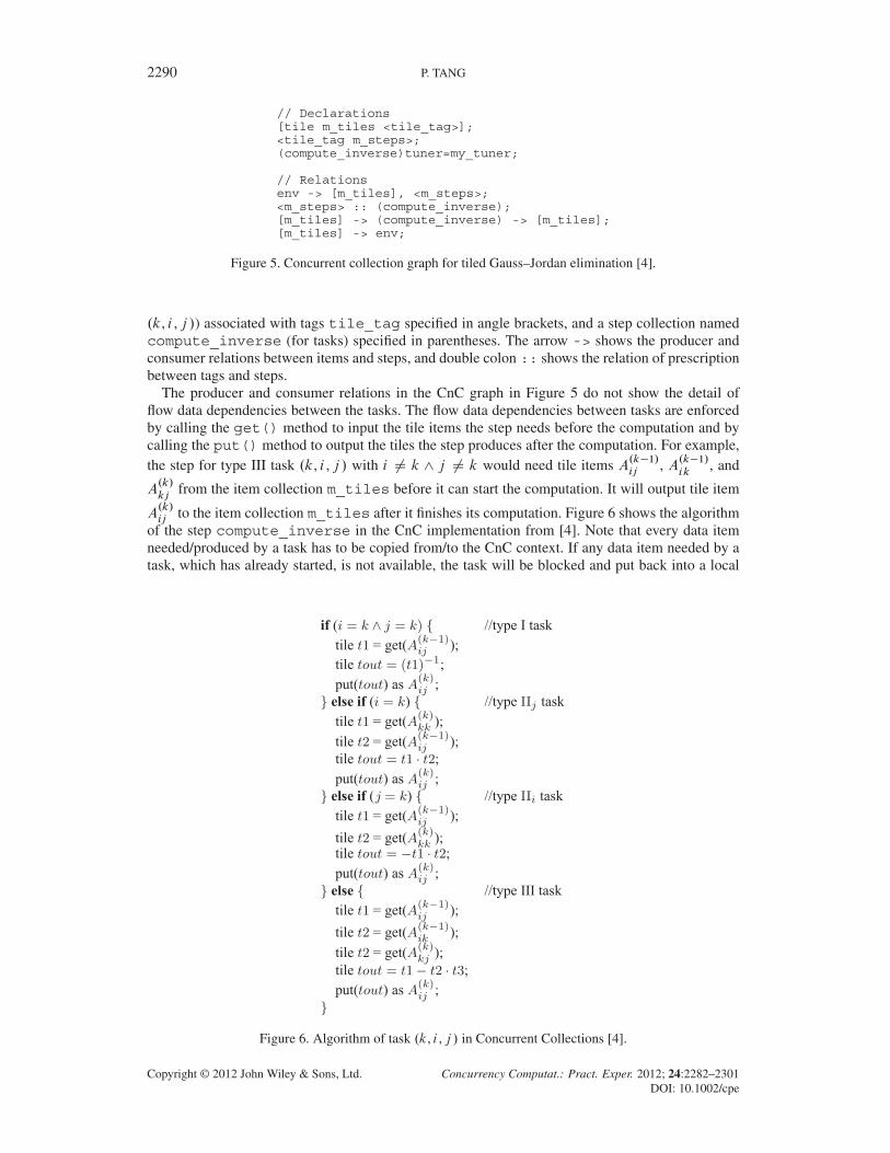
flow data dependencies between the tasks. The flow data dependencies between tasks are enforcedby calling the get() method to input the tile items the step needs before the computation and bycalling the put() method to output the tiles the step produces after the computation. For example,the step for type III task .k, i , j / with i ¤ k ^ j ¤ k would need tile items A

.k�1/ij , A

.k�1/

ik, and

A.k/

kjfrom the item collection m_tiles before it can start the computation. It will output tile item

A.k/ij to the item collection m_tiles after it finishes its computation. Figure 6 shows the algorithmof the step compute_inverse in the CnC implementation from [4]. Note that every data itemneeded/produced by a task has to be copied from/to the CnC context. If any data item needed by atask, which has already started, is not available, the task will be blocked and put back into a local

Figure 6. Algorithm of task .k, i , j / in Concurrent Collections [4].



queue. The blocked task will be rescheduled to the ready queue of the thread when it gets all thedata items it needs [17]. This is obviously inefficient if the task has to be rescheduled many times.So, CnC provides a tuner [4] class, which allows programmers to spell out the data items that atask needs so that the scheduler will not schedule the task until all the data items it needs are avail-able. We run CnC code both with and without the tuner in our experimentation to see the differencebetween their performances.Another important optimization in CnC is the memory management of single-assignment data

items [18]. Because CnC does not know how many steps (tasks) will read a data item (through theget() method), it will keep the data item indefinitely, and the memory usage would be exploded.CnC allows programmers to pass the number of the tasks that would read the data item, called thereference count, as an argument to the put() method when the data item is output to the context.The reference count will be decremented whenever get() is called. The storage of the data item isgarbage collected when its reference count reaches zero. We always turn this optimization on whenwe run the CnC code. The details of the CnC implementation of tiled Gauss–Jordan elimination canbe found in [4].

4. IMPLEMENTATION IN THREADING BUILDING BLOCKS

Threading Building Blocks allows one to build and evaluate task graphs by using the referencecount, ref_count, of the task class of TBB. In particular, the task graph can be built by

1. Setting up the ref_count of each task to the number of its predecessors.2. Inserting the code to decrement the ref_count of each of its successors towards the end ofthe task and spawn the successor if its ref_count reaches zero after the decrement.

Spawning a task is to put it in the task queue of the physical thread. The TBB scheduler willpick up the tasks in the ready queue of the physical thread to run. TBB uses work-stealing schedul-ing, and load balance is achieved by letting idle threads steal tasks from the ready queues of otherphysical threads.We can add an additional empty task to the graph to be the successor of all the tasks that do not

have successors in the original graph. To evaluate and execute the graph, the main driver simplyspawns the tasks that do not have predecessors and wait on the added empty task. The tasks will beexecuted in the order prescribed by the edges of the task graph because a task will not be put in thetask queue of a physical thread until its ref_count becomes zero, and its ref_count reacheszero only if all of its predecessor tasks are completed.Because TBB accesses and updates the tile array Aij (0 6 i , j 6 d � 1/ directly, the task

graph has to include all the flow, anti, and output data dependencies described in Section 2.For this Gauss–Jordan elimination algorithm, the output data dependencies are subsumed by theflow data dependencies, and we only need to include the flow and anti data dependencies in thetask graph.The implementation has two classes: task_graph for the task graph and DagTask for

the task as a subclass of TBB task class tbb::task. The build-graph() method (of thetask_graph class) is to build the task graph. Its pseudocode is shown in Figure 7. It basically cre-ates d 3 tasks .k, i , j / (0 6 k, i , j 6 d � 1) referenced by m_tasksŒk�Œi �Œj �. For each task, it calcu-lates the number of flow and anti data dependency predecessors according to the Lemmas in Tables IIand IV and stores them in variables flow_dep_count and anti_dep_count, respectively. Itfinally sets the ref_count of the task m_tasksŒk�Œi �Œj � with the sum of flow_dep_countand anti_dep_count.The computation of a TBB task is specified in its execute() method. Pseudocode of the

execute() method of the DagTask task is shown in Figure 8. It first executes the computa-tion according to the type of the task determined by its index .k, i , j / as summarized in Table I. Thetask reads the tiles that it needs and writes the tile it calculates directly. There is no copying of tilesback and forth as in the CnC implementation. The second part of execute() is to decrement theref_count of each of its flow and anti data dependency successors determined by the Lemmas in


2292 P. TANG

Figure 7. Algorithm of build-graph() of task_graph.

Tables III and V, respectively. If the ref_count of any successor is zero after the decrement, thetask spawns that successor, putting it in the task queue of the physical thread.

5. OVERHEAD OF CONCURRENT COLLECTIONS OVER THREADING BUILDINGBLOCKS FOR GAUSS–JORDAN ALGORITHM

To measure the overhead of CnC over TBB, we run the TBB and CnC implementations on anOctal-core AMD Opteron(tm) 2.8 GHz 8220 processor with 64 GByte memory and 1024KB cacheand 1024 TLB for 4K pages in each core. We vary the number of cores to use from 1 to 8 forproblem sizes from 1024 to 5120. We also run the sequential tiled Gauss–Jordan elimination inFigure 1 as the base sequential time in calculating speedups of parallel executions. To see the impactof the tile size on performance and find the best tile size, we vary the tile size from 8 to 256. Foreach configuration, we run the code five times and take the average of the execution times as itsexecution time.The execution times of problem size 2048 with different tile sizes t ranging from 8, 16, � � � to 256

of TBB and CnC with and without tuner are shown in Figures 9(a), 9(b), and 9(c), respectively.We calculated the GFLOPS by dividing the number of floating-point operations flop.n, t / by the

execution time as follows:

GFLOPS.n, t / D flop.n, t /

109 � e.n, t /(3)

where flop.n, t / is as shown in (1) and e.n, t / is the execution time in seconds for problem size n

and tile size t . The GFLOPS for TBB, CnC with tuner, and CnC without tuner for problem size2048 is shown in Figures 10(a), 10(b), and 10(c), respectively.Figure 11 shows the speedup over the sequential execution time calculated by the following:

Snp.n, t / D es.n, t /

enp.n, t /(4)

where es.n, t / is the execution time of the sequential algorithm in Figure 1 and enp.n, t / is the par-allel execution for problem size n and tile size t . The speedups of TBB, CnC with tuner, and CnCwithout tuner for problem size 2048 are shown in Figures 11(a), 11(b), and 11(c), respectively.



Figure 8. Algorithm of execute() for task .k, i , j / in Threading Building Blocks.

5.1. Performance analysis

We first observed in Figures 9(a), 9(b), and 9(c) that the sequential execution time seq (i.e., es.n, t /)decreases as tile size t increases from 8 to 64. It then increases sharply from 15.12 to 37.26 (2.46fold increase) when t changes from 64 to 128, although the number of floating-point operationsdecreases as the tile size increases according to (1). This is because of the degradation of cache hitratio when the tile size crosses from 64 to 128 [11]. This is true for all other problem sizes. We


2294 P. TANG

0

10

20

30

40

50

60

70

80

90

2561286432168E

xecu

tion

Tim

e in

Sec

onds

Tile Size

TBB Times with Different Tile Sizes for Problem Size 2048

seqnp=1np=2np=3np=4np=5np=6np=7np=8

(a) TBB Execution Time

0

10

20

30

40

50

60

70

80

90

2561286432168

Exe

cutio

n T

ime

in S

econ

ds

Tile Size

CnC Times with Different Tile Sizes for Problem Size 2048


(b) CnC with Tuner Execution Time

0

10

20

30

40

50

60

70

80

90

2561286432168

Exe

cutio

n T

ime

in S

econ

ds

Tile Size

CnC Times without Tuner for Problem Size 2048


(c) CnC without Tuner Execution Time

Figure 9. Execution time for problem size 2048. (a) Threading Building Blocks (TBB) execution time, (b)Concurrent Collections (CnC) with tuner execution time, and (c) CnC without tuner execution time.

calculated the ratio e.n,128/e.n,64/

for all problem sizes n D 1024, 2048, 3074, 4096, and 5120, and theyare all around 2.46. This confirms the cache miss analysis in [11] and gives us 64 as the best tile sizefor our machine.The np=1 time in Figures 9(a), 9(b), and 9(c) is the parallel execution time using one core. The

gap between the np=1 time and the sequential time seq is the overhead of the parallel code overthe sequential code. We observed that the smaller the tile size, the larger this gap. This is becausesmaller tile sizes generate more tasks in the task graph that need to be scheduled. The gap between



0

1

2

3

4

5

6

7

8

9

2561286432168Gig

a Fl

oatin

g-Po

int O

pera

tions

per

Sec

ond

Tile Size

TBB GFLOPS for Problem Size 2048


(a) TBB GFLOPS

0

1

2

3

4

5

6

7

8

9

2561286432168Gig

a Fl

oatin

g-Po

int O

pera

tions

per

Sec

ond

Tile Size

CnC GFLOPS with Tuner for Problem Size 2048


(b) CnC With Tuner GFLOPS

0

1

2

3

4

5

6

7

8

9

2561286432168Gig

a Fl

oatin

g-Po

int O

pera

tions

per

Sec

ond

Tile Size

CnC GFLOPS without Tuner for Problem Size 2048


(c) CnC Without Tuner GFLOPS

Figure 10. Giga floating-point operations per second (GFLOPS) performance for problem size 2048. (a)Threading Building Blocks (TBB) GFLOPS, (b) Concurrent Collections (CnC) with tuner GFLOPS, and (c)

CnC without tuner GFLOPS.

np=1 time and seq time in CnC is larger than TBB (see Figs. 9(a) and 9(b)). For the CnC withouttuner, this gap is so large that all the parallel execution times using 1, 2, � � � , 8 cores for tile sizes 8and 16 are greater than the sequential time (see Figure 9(c)). Also, notice that for tile size 128, TBBtime using one core is a bit less than the sequential time (see Figure 9(a)). This may be because ofthe fact that TBB uses its own efficient memory allocator [5, 6, 19], and this is the reason for thesuper-liner speedup of TBB for tile size 128 (see Figure 11(a)).


2296 P. TANG

0

1

2

3

4

5

6

7

8

1 2 3 4 5 6 7 8Sp

eedu

p ov

er T

iled

Sequ

entia

l Tim

e

The Number of Cores Used

Speedup of TBB for size 2048

linear speedupspeedup 1

ts=8ts=16ts=32ts=64

ts=128ts=256

(a) TBB Speedup

0

1

2

3

4

5

6

7

8

1 2 3 4 5 6 7 8

Spee

dup

over

Tile

d Se

quen

tial T

ime


Speedup of CnC for size 2048


ts=8ts=16ts=32ts=64

ts=128ts=256

(b) CnC with Tuner Speedup

0

1

2

3

4

5

6

7

8

1 2 3 4 5 6 7 8

Spee

dup

over

Tile

d Se

quen

tial T

ime


Speedup of CnC without Tuner for size 2048


ts=8ts=16ts=32ts=64

ts=128ts=256

(c) CnC without Tuner Speedup

Figure 11. Speedup for problem size 2048. (a) Threading Building Blocks (TBB) speedup, (b) ConcurrentCollections (CnC) with tuner speedup, and (c) CnC without tuner speedup.

The speedups with tiles sizes 128 and 256 are higher than the tile size 64. The reason is that poorcache performance makes the task execution time 2.46 times greater and that amortizes the schedul-ing overhead of the parallel execution. But, the tile sizes 128 and 256 have very low GFLOPS (seeFigures 10(a), 10(b), and 10(c)).For the optimal tile size 64, the speedup over sequential time for TBB, CnC with tuner, and CnC

without tuner using eight cores are 7.52, 6.62, and 6.22, respectively. The GFLOPS performances of



TBB, CnC with tuner, and CnC without tuner using eight cores are 8.61, 7.57, and 7.12 GFLOPS,respectively.

5.2. Measuring the overhead of Concurrent Collections

To measure the overhead of CnC over TBB, we calculated the CnC/TBB ratio as follows:

RCnC=TBB D eCnC.n, t /

eTBB.n, t /(5)

where eCnC.n, t / and eTBB.n, t / are the CnC and TBB execution times, respectively.The CnC/TBB ratios, RCnC=TBB, for different tile sizes and problem size n D 2048 are plotted

in Figure 12. Figures 12(a) and 12(b) are the ratios of the CnC with and without tuner over TBB,respectively. The CnC/TBB ratios for tile size 8, 16, and 32 without tuner are very large and out ofthe y-range in the plot in Figure 12(b). For the optimal tile size 64, the CnC/TBB ratio is increasingwith the number of cores used. For the CnC with tuner, the CnC/TBB is between 1.10 (using 1 core)and 1.14 (using 8 cores), or the overhead CnC over TBB is between 10% and 14% of TBB time (seeFigure 12(a)). For the CnC without tuner, the CnC/TBB ratio for tile size 64 is between 1.17 (using1 core) and 1.21 (using 8 cores), with the CnC overhead between 17% and 21% of TBB time (seeFigure 12(b)).

1

1.1

1.2

1.3

1.4

1.5

1 2 3 4 5 6 7 8CnC

(with

Tun

er)/

TB

B E

xecu

tion

Tim

e R

atio


CnC(with Tuner)/TBB Execution Time Ratio for size 2048

ts=8ts=16ts=32ts=64

ts=128ts=256

(a) CnC (withTuner)/TBB Ratio

1

1.1

1.2

1.3

1.4

1.5

1 2 3 4 5 6 7 8

CnC

(with

out T

uner

)/T

BB

Exe

cutio

n T

ime

Rat

io


CnC(without Tuner)/TBB Execution Time Ratio for size 2048

ts=8ts=16ts=32ts=64

ts=128ts=256

(b) CnC (withoutTuner)/TBB Ratio

Figure 12. Concurrent Collections (CnC)/Threading Building Blocks (TBB) execution time ratio forproblem size 2048. (a) CnC (with tuner)/TBB ratio and (b) CnC (without tuner)/TBB ratio.


2298 P. TANG

0

1

2

3

4

5

6

7

8

9

10

10240921681927168614451204096307320481024G

iga

Floa

ting-

Poin

t Ope

ratio

ns p

er S

econ

dProblem Size

GFLOPS using 8 Cores with Best Tile Size 64

TBBCnC with Tuner

CnC without TunerSequential

(a) GFLOPS using 8 Cores with Tile Size 64

1

1.05

1.1

1.15

1.2

1.25

1.3

1.35

1.4

10240921681927168614451204096307320481024

CnC

/TB

B E

xecu

tion

Tim

e R

atio

Problem Size

CnC/TBB Execution Time Ratio for Tile Size 64

CnC with TunerCnC without Tuner

(b) CnC/TBB Ratio using 8 Cores with Tile Size 64

0

0.1

0.2

0.3

0.4

0.5

0.6

0.7

0.8

0.9

1

10240921681927168614451204096307320481024

TB

B/C

nC E

xecu

tion

Tim

e R

atio

Problem Size

TBB/CnC Execution Time Ratio for Tile Size 64

CnC with TunerCnC without Tuner

(c) TBB/CnC Ratio using 8 Cores with Tile Size 64

Figure 13. Performance of the optimal tile size 64 using eight cores. (a) Giga floating-point operations persecond (GFLOPS) using eight cores with tile size 64, (b) Concurrent Collections (CnC)/Threading BuildingBlocks (TBB) ratio using eight cores with tile size 64, and (c) TBB/CnC ratio using eight cores with tile

size 64.

Because the tile size 64 gives the best performance, we run the TBB, CnC with and withouttuner implementations, as well as the sequential code using eight cores for the problem sizes of6144–10240 with fixed tile size 64.We calculated their GFLOPS according to (3) and plotted the GFLOPS for tile size 64 for all the

problem sizes of 1024–10240 in Figure 13(a). We also calculated the CnC/TBB ratios according to(5), which is equivalent to GFLOPSTBB.n,t/

GFLOPSCnC.n,t/and plotted them in Figure 13(b). Figure 13(a) shows



that the GFLOPS of TBB is consistently higher than those of CnC. All the GFLOPS increase withthe increasing problem size. Figure 13(b) shows that the CnC/TBB time ratio is between 1.15 and1.12 for the CnC with tuner and between 1.22 and 1.18 for the CnC without tuner. All the CnC/TBBratios decrease as the problem size increases. The overhead of CnC over TBB is between 12% and15% with tuner and between 18% and 22% without tuner.We also calculated GFLOPSCnC.n,t/

GFLOPSTBB.n,t/, which is the reciprocal of the CnC/TBB ratio, called the

TBB/CnC ratio and plotted them in Figure 13(c). The TBB/CnC ratio or GFLOPSCnC.n,t/GFLOPSTBB.n,t/

showsthe percentage of the TBB performance that CnC can deliver. Figure 13(c) shows the CnC withtuner that can deliver as much as 87%-89% of the TBB performance and the CnC without tuner thatdelivers 82%-85% of the TBB performance.

6. RELATED AND FUTURE WORK

Comprehensive performance evaluation of CnC is reported in [16]. It compares the performanceof CnC with that of OpenMP with Math Kernel Library (MKL), Cilk, Multi-threaded MKL,ScaLAPACK with shared memory Message Passing Interface (MPI), and PLASMA with MKL onCholesky factorization and Eigensolver problem. It shows that CnC is comparable with PLASMAwith MKL, which also uses the task graph-based approach of parallel execution, and CnC is superiorto all the loop-based OpenMP with MKL, Cilk, Multi-threaded MKL and ScaLAPACK with sharedmemory MPI. In this paper, we compared both task-based CnC and TBB and showed that TBB is12%–15% faster than CnC on Gauss–Jordan elimination.The parallel Gauss–Jordan elimination reported in [12] is loop-based like the one in Figure 3.

The work of [16] already showed that loop-based parallel algorithms are always inferior to thetask-based algorithm in CnC on the Cholesky factorization and the Eigensolver problem. In thispaper, we showed that the task-based algorithm in TBB is about 12%–15% faster than CnC onthe Gauss–Jordan elimination. The superior performance of task-based algorithms to the loop-based algorithms in LAPACK or MKL is also reported in [14] on QR factorization and in [15] onCholesky factorization.Both parallel tiled Gauss–Jordan algorithms reported in [12] and [13] are restricted on the aug-

mented system using two data arrays. Our parallel Gauss–Jordan algorithm is an in-place algorithmstoring the inverted matrix in the same tiled data array of the input matrix.Our experiments also confirm the analysis of the impact of tile size on cache performance in [11]

and found the best tile size for our machine.Parallel programming of the loop-based parallel Gauss–Jordan algorithm shown in Figure 2

in TBB will be much simpler than the task-based TBB programming shown in this paper. Thetask-based programming in CnC is also much simpler than the task-based programming in TBB.One future work would be to implement and compare the performances of the task-based parallelGauss–Jordan algorithm in CnC with a loop-based one in TBB.Another future work is to compare the performances of Gauss–Jordan elimination in TBB,

CnC, and OpenMP (both task-based and loop-based) because OpenMP now supports task-basedprogramming as well.We also plan to test the scalability of CnC and TBB for parallel Gauss–Jordan elimination using

Intel processors with larger number of cores in the future.

7. CONCLUSION AND DISCUSSION

We make the following contributions in this paper: (i) we provided a complete data dependencyanalysis for the tiled in-place Gauss–Jordan elimination algorithm to guide task-based paralleliza-tion; (ii) we parallelized and implemented the tiled in-place Gauss–Jordan elimination in TBB; and(iii) we compared the task-based parallel performances of CnC and TBB and found that the over-head of CnC, which is implemented on top of TBB, is only within 12%–15% of the TBB executiontime for the CnC with tuner and 18%–22% of the TBB execution time for the CnC without tuner.


2300 P. TANG

The overheads of CnC over TBB mentioned previously can be translated to that the CnC withtuner delivers 87%–89% of the TBB performance, and the CnC without tuner delivers 82%–85% ofthe TBB performance.Task-based parallelizing and programming in CnC is easier for two reasons. Firstly, CnC pro-

gramming does not need to analyze anti and output dependencies because its data flow single-assignment model eliminates all of them. Secondly, The flow dependencies are enforced and speci-fied through the data items that carry the data flow. This can be simply done by calling the get()method for each data item that the task needs. Using tuner in CnC is not difficult either: all thatis needed is to specify all the data items the task needs. The data items that a task needs can beeasily identified from the code of the task. (However, the memory management optimization ofCnC [18] requires one to know the number of tasks that would read the data item, which is thesame as the number of flow data dependency successors of the task writing the item. This requires aflow dependency analysis.) In contrast, task-based parallelizing and programming in TBB requiresa full data dependency analysis, including the output and especially the complicated anti datadependency analysis.Given that CnC with tuner can still deliver 87%–89% of the TBB performance and TBB requires

the complex data dependency analysis, we believe that CnC is very promising in winning acceptanceby parallel programmers for dense linear algebra algorithms in the future.

ACKNOWLEDGEMENT

The work is supported in part by equipment purchased under NASA Award NCC5-597.

REFERENCES

1. Anderson E, Bai Z, Bischof C, Blackford S, Demmel J, Dongarra J, Du Croz J, Greenbaum A, Hammarling S,McKenney A, Sorensen D. LAPACK User’s Guide. SIAM: Philadephia, PA, 1999.

2. Agullo E, Hadri B, Ltaief H, Dongarrra J. Comparative study of one-sided factorizations with multiple softwarepackages on multi-core hardware. In Proceedings of the Conference on High Performance Computing Networking,Storage and Analysis SC ’09. ACM: New York, NY, USA, 2009; 20:1–20:12.

3. Haidar A, Ltaief H, YarKhan A, Dongarra J. Analysis of dynamically scheduled tile algorithms for dense linearalgebra on multicore architectures. Technical Report Tech. Rep. ut-cs-11-666, Innovative Computing Laboratory,University of Tennessee, 2011.

4. CnC Team. Intel Concurrent Collections for C++. Technical Report, Intel Inc., 2009. http://software.intel.com/en-us/articles/intel-concurrent-collections-for-cc/.

5. Reinders J. Intel Threading Building Blocks: Outfitting C++ for Multi-core Processor Parallelism, Oreilly Associates,2007.

6. Reinders J. TBB 3.0: New (today) version of Intel Threading Building Blocks. Technical Report, IntelInc., May 2010. http://software.intel.com/en-us/blogs/2010/05/04/tbb-30-new-today-version-of-intel-threading-building-blocks/.

7. Arvind, Gostelow KP, Plouffe W. An asynchronous programming language and computing machine. TechnicalReport Tech. Rep. TR 114a, University of California at Irvine, 1978.

8. Carriero N, Gelernter D. Linda in context. Communications of the ACM April 1989; 32:444–458.9. Knobe K. Ease of use with Concurrent Collections (CnC). In Proceedings of the First USENIX conference on Hot

topics in parallelism, HotPar’09. USENIX Association: Berkeley, CA, USA, 2009; Article 17.10. Chandramowlishwaran A, Knobe K, Vuduc R. Applying the concurrent collections programming model to asyn-

chronous parallel dense linear algebra. In Proceedings of the 15th ACM SIGPLAN symposium on Principles andpractice of parallel programming, PPoPP ’10. ACM: New York, NY, USA, 2010; 345–346.

11. Park N, Hong B, Prasanna VK. Tiling, block data layout, and memory hierarchy performance. IEEE Transactions onParallel and Distributed Systems July 2003; 14:640–654.

12. Melab N, Talbi E-G, Petiton S. A parallel adaptive Gauss-Jordan algorithm. Journal of Supercomputing September2000; 17:167–185.

13. Shang L, Petiton S, Hugues M. A new parallel paradigm for block-based Gauss-Jordan algorithm. In Proceedings ofthe 2009 International Conference on Grid and Cooperative Computing, 2009; 193–200.

14. Buttari A, Langou J, Kurzak J, Dongarra J. Parallel tiled QR factorization for multicore architectures. Concurrencyand Computation: Practice and Experience September 2008; 20:1573–1590.

15. Buttari A, Langou J, Kurzak J, Dongarra J. A class of parallel tiled linear algebra algorithms for multicorearchitectures. Parallel Computing January 2009; 35:38–53.

16. Chandramowlishwaran A, Knobe K, Vuduc R. Performance evaluation of concurrent collections on high-performance multicore computing systems. In Proceedings of the 2010 IEEE International Symposium on Paralleland Distributed Processing (IPDPS), April 2010; 1–12.



17. Chandramowlishwaran A, Knobe K, Lowney G, Sarkar V, Treggiari L. Multi-core implementations of the concurrentcollections programming model. In The 14th Workshop on Compilers for Parallel Computing (CPC), January 2009.

18. Budimlic Z, Chandramowlishwaran AM, Knobe K, Lowney GN, Sarkar V, Treggiari L. Declarative aspects of mem-ory management in the concurrent collections parallel programming model. In Proceedings of the 4th workshop onDeclarative aspects of multicore programming, DAMP ’09. ACM: New York, NY, USA, 2008; 47–58.

19. Kukanov A, Voss M. The foundations for scalable multi-core software in Intel Threading Building Blocks. IntelTechnology Journal November 2007; 11:309–322.


Documents

Measuring the overhead of Intel C++ Concurrent … the overhead of Intel C++ Concurrent Collections over Threading Building Blocks for Gauss–Jordan ... the ease of programming and