Measuring the Gravitational Constant with a Torsion

Balance

Jason R. Heimann

with

John Wray

November 12, 2004

i

Contents

1 Introduction 1

2 Experimental Apparatus 1

2.1 Torsion Balance and Readout . . . . . . . . . . . . . . . . . . . . . . . . . . . 12.2 Vibration Isolation Table . . . . . . . . . . . . . . . . . . . . . . . . . . . . . 22.3 Laser and Optics . . . . . . . . . . . . . . . . . . . . . . . . . . . . . . . . . . 22.4 Other Measurements . . . . . . . . . . . . . . . . . . . . . . . . . . . . . . . . 3

3 Procedure 3

3.1 Setup . . . . . . . . . . . . . . . . . . . . . . . . . . . . . . . . . . . . . . . . 33.2 Measurement . . . . . . . . . . . . . . . . . . . . . . . . . . . . . . . . . . . . 3

4 Results 4

5 Analysis and Interpretation 4

5.1 Theory . . . . . . . . . . . . . . . . . . . . . . . . . . . . . . . . . . . . . . . . 45.2 Experiment . . . . . . . . . . . . . . . . . . . . . . . . . . . . . . . . . . . . . 7

6 Conclusion 7

7 Tables and Figures 8

ii

1 Introduction

The inquisition for the Higgs particle is the current manifestation of mankind’s yearning tounderstand gravitation. Over four hundred years ago Isaac Newton performed research withmacroscopic and astronomical objects to build the basis of gravitational theory. In 1665, atage 23, Newton “showed that the force that holds the Moon in its orbit is the same forcethat makes an apple fall.”[2] In his proposition is a force law known now as Newton’s Lawof Gravitation:

FG = Gm1m2

r2(1)

The law states that every body attracts every other body with a force whose magnitudeis given by equation 1. This force includes a constant G called the universal constant ofgravitation.

Early tests of Newton’s law involved measuring the “Attraction of Mountains” since verylarge masses were required to produce an appreciable deflection of measurement equipmentavailable at the time. This is a consequence of the extreme weakness of the gravitational forceat the human scale. In comparison to one’s attraction to Earth, forces due to nearby massesare inconsequential. With this in mind, a very delicate piece of equipment was designedand built by the Revd. John Michell that could measure very weak forces. UnfortunatelyMichell died before he could use his own design in an experiment.

Despite its name, Cavendish’s experiment was made possible through the work of as-tronomers, geologists, mathematicians and other scientists that came before him. To hiscredit, Henry Cavendish was the diligent chap that obtained the final result of the exper-iment; Cavendish completed the measurement in 1798, five years after Michell’s death.[1]His diligence in experimental techniques and error determinations has lead some to callthis experiment the “first modern physics experiment.”[4] As a testament to this claim,Cavendish’s results from this experiment were not improved for over a century.

2 Experimental Apparatus

The apparatus used in our experiment is much like that which was used by Cavendish; weuse a torsion balance with an optical method of measurement. In our case the optics areimproved (incorporating a He-Ne laser) and the read out is supplemented by a PC-basedDAQ system. We also improved the isolation of our experiment with an active vibrationdamping system.

2.1 Torsion Balance and Readout

Central to the experiment is the torsion balance. The balance used in our experiment ispictured in figure 1. This design incorporates clever use of symmetry to prevent the Earth’sgravitational force from adversely affecting its measurement. It is extremely sensitive totorsional forces; since it incorporates a tungsten thread as its torsion element, it offers onlya very faint resistance to movement. The torsion element is also sensitive to environmentalconditions including temperature and air flow. To protect the balance from external contactand air flow it is encased in an aluminum structure with removable glass windows.

1

Our balance is fundamentally the same as that which was used in Cavendish’s experi-ment: a suspended boom with two small lead spheres in axial alignment with a boom withtwo larger lead spheres. The boom with the large weights is fixed along two axes to preventany pendulous movements; this outer boom can only be rotated along the same axis as thesuspended boom. The suspended boom hangs freely from ∼6 cm of tungsten thread. Thisthread is carefully tied to upper and lower posts, each allowing for some adjustment. Theupper post allows one to raise and lower the inner boom, and rotate it along the verticalaxis. The lower post slides and rotates within a groove in the suspended boom.

Our balance allows two different methods of readout. A small mirror is fixed to the centerpost of the balance for use as an “optical lever.” A symmetric differential capacitive sensoris built into the base of our balance to provide an analog readout. This output provides asignal whose voltage varies as the inner balance rotates. The sensor is especially resistantto pendulous modes (see figure 2 for a graphical explanation) of motion and electrical noise.

An external piece of DAQ hardware (also pictured in figure 1) provides power to thereadout electronics and allows for zero-adjustment of the signal from the balance. Thishardware feeds the signal to a DAQ card in a PC that records the voltage in two secondintervals. Measurements are output in a text file that is analyzed with statistical softwareincluding ROOT and Gnuplot.

2.2 Vibration Isolation Table

We employ a vibration isolation table in this experiment to minimize errors in measurementcaused by forces external to our apparatus. We also wanted to minimize movements in thesuspended boom, as our theoretical model of this experiment does not account for suchmotion. The table also provides us (once properly adjusted) with a very uniform and levelsurface. This also improves our experiment’s correlation to our theoretical model, whichassumes the apparatus is perfectly aligned with the horizon.

The table is a large aluminum slab that rests on four pneumatic pistons. Attached toeach piston is a small lever with an adjustable foot that rests against the bottom of the slab.As the slab moves up and down, the lever tracks its movement and adjusts the valve thatregulates the corresponding piston’s internal pressure. An air compressor with reservoirsits adjacent to the table, sourcing the levelling pistons. The compressor has an automaticregulator that runs the pump as needed to maintain sufficient pressure in the reservoir.

2.3 Laser and Optics

A 0.6 mW Helium-Neon laser made by Uniphase (Model 1508) was incorporated to producean “optical lever” arrangement. Figure 3 illustrates our arrangement; note the error of +/-0.7 cm in the measurements. Our primary concern during our design phase was accuracy ofmeasurement. We aimed to minimize the laser-mirror distance to minimize effects of beamspread, and maximize the mirror-yardstick distance to maximize our angular resolution.Another factor minimizing beam spread was a small convex lens held in position by a labstand. A jack stand was used to center the laser beam within the small mirror on the centerpost (seen in figure 2).

2

2.4 Other Measurements

We weighed the lead spheres with a triple-beam balance and measured their diameters witha vernier caliper. The caliper was also used to measure dimensions of the balance. Theyardstick in figure 3 is fixed to the wall with double-stick tape, and a thin strip of blackmasking tape is affixed to the portion of the ruler on which the laser beam is incident. Theuse of black tape reduced the glare from the incident beam, allowing for (slightly) moreprecise measurement.

3 Procedure

3.1 Setup

Our first task was to ensure our apparatus had a level surface on which to rest. We openedthe air valves to all of the pistons under the isolation table and allowed them to fill untilthe adjustment lever stopped the flow. We then used a small circular level to check thepitch of the table at various locations. After adjusting the feet on the levers, we achieveda uniformly level table. We set up our equipment as in figure 3 and left it alone overnightso all motion within our balance ceased. The next day we levelled our torsion balance viaadjustable feet on the balance’s base. The circular level indicated we had a level balance,now assumed to be an the same plane as our table.

Upon further inspection, we found the suspended boom was not properly aligned withthe center post. Using a small pin, John pushed the boom from side to side through smallholes in either side of our balance’s enclosure. After some work we left the system alone foranother night. Later, we verified the suspended boom appeared to be parallel with the table,but the boom’s equilibrium point was at some large angle to the glass walls of the balance.The upper support was carefully adjusted several times before we achieved a centered boom(note our “centering” here is not exact; this was a difficult task and we allowed for about 5degrees of error in our determination of “center”). We noted the mirror on the center postwas not parallel to the boom, so we corrected for this misalignment by rotating the entirebalance. After more settling time we verified we had achieved our intended beam path.

After affixing the yardstick to the far wall and masking it with black tape, we attemptedto minimize the beam spot size (to aid measurement) by incorporating a convex lens in thestationary portion of the beam. We avoided putting the lens in the moving portion of thebeam to minimize errors caused by optical aberration. While adjusting the position of thelens in the beam, we noticed the spot size at the yardstick shrank as the lens approachedthe balance. We could only move the lens a certain amount, however, since at some pointthe reflected beam strikes the edge of our lens. Our final configuration was measured andthe results appear as dimensions in our schematic (figure 3).

3.2 Measurement

Our DAQ software was simple to operate, although its interface was far from intuitive. Wesimply turned the software “on” and let it run, and it would record the signal level from ourbalance once every two seconds. We placed the large masses in position I (see figure 4 for aplan view of the positions) and recorded data as the torsion balance settled into equilibrium

3

over a 24 hour period. As shown in figure 6, the equilibrium position of the balance changedover time. With this in mind we decided to record only about an hour of data for eachadjustment of the large masses.

In our final data run we performed two measurements in position II and one measurementin position I. Each measurement began with a “swap” in position of the large masses (fromI to II or II to I) and ended about an hour later. Before swapping the large masses we notedthe position of the laser beam by making a pencil mark where the center of the beam wasincident on the yardstick. We later used a vernier caliper to measure the distance betweenour marks, as well as the apparent size of the laser beam.

At the conclusion of our balance measurements we recorded the dimensions of the balanceand masses for use in the determination of our final result. Since the masses were notuniformly spherical we took several diameter measurements for each sphere and used anaverage result in our calculations. Some dimensions could not be directly measured withthe caliper (i.e. with the jaws of the caliper touching the apparatus), so we held the caliperup to the dimension in question and aligned the jaws with the apparatus by “eyeball.”This introduced some uncertainty due to parallax; we accounted for our gross measurementtechnique in our determination of measurement uncertainty.

4 Results

An enormous amount of raw data (over 6,300 data points in our final run) was collectedduring the course of our experiment. To save patience and paper, we present only portionsof raw data that are relevant to our final result. Furthermore our raw data will only appearin graphical form. Numerical values that appear in the following tables are results of fittingalgorithms or analytical manipulations thereof.

Figure 6 is our first sample of data from the experiment. Shortly after this data wasgathered we made our final data run; see figure 7 for our final results with the balance.For reference, time “0” in our data set corresponds to November 3, 2004 6:30:09 PM PST.Our measurements of the spheres’ diameters appear in table 1 and the rest of our balance’sdimensions are shown in table 2.

5 Analysis and Interpretation

5.1 Theory

The theoretical model of our experiment include many assumptions, made to simplify theequations used in determining G:

• Only two equal and opposite forces are acting to torque our balance’s suspended boom.There is no drag or friction experienced within the balance.

• Our balance is perfectly symmetric:

– The large and small masses are perfectly spherical.

– The large spheres have identical masses; the small spheres have identical masses.

4

– The separation between the large and small spheres is identical for both equilib-rium positions (I and II) and for both sides of our balance.

– The large spheres are positioned such that the lever arm of its attractive force isat a right angle to the boom and in a plane perpendicular to the thread.

– The suspended boom moves only in a plane perpendicular to the thread.

• The suspended boom is parallel to the glass windows when the sphere separationdistance is determined.

• We can neglect the gravitational and inertial effects of the suspended boom and centerpost.

• We can neglect the gravitational effect of the outer boom.

• We can neglect any other external gravitational effects, such as the attractive force ofthe nearby experimentalists.

Correction factors can be derived to account for all of our assumptions, however, thesefactors can be negligible compared to the accuracy of our measurements. We will use onlyone correction factor in our determination of G.

As described above, we have two forces acting within our balance: the attraction of thenearby large mass, and the restoring force of the torqued thread. Individually, these forcesare:

τG = 2FGd (2)

τκ = −κθ (3)

In opposition, these forces equate as τG = −τκ. Including equation 1 this gives us thesteady-state equation

κθ = 2dGmlms

r2(4)

which we can rearrange to determine G. We also define b as the sphere separation distance(see figure 4).

G =κθb2

2dmlms

(5)

The two unknowns in this equation are κ and θ. We use geometrical analysis to reduceθ to a linear variable (see figure 5): making the small-angle approximation θ ≈ tanθ weachieve a relation to the beam displacement ∆S. Keep in mind the θ we observe is actuallytwice the rotation angle of the boom, due to the law of reflection.

2θ =∆S

2L or θ =

∆S

4L(6)

The torsional spring constant κ is determined from the solution to classical mechanics’infamous simple harmonic oscillator problem:

ω0 =2π

T0=

√

κ

I(7)

5

As stated in our assumptions, we will model the suspended boom as massless and onlyconsider the small spheres in determining I.

I = 2ms(d2 +

2

5r2) (8)

Combining equations 7 and 8 and solving for κ, we achieve our spring constant:

κ = 2ms(d2 +

2

5r2)ω2

0 (9)

It should be noted that our balance is a damped simple harmonic oscillator; its behavior ismodeled with the following solution:

V (t) = Ae−β(t−t0)cos(ω1(t − t0) − δ) + C (10)

We define an offset time t0 at which oscillation begins, and a phase factor δ. Since ourdamping is small (<5%, see table 3 for an example) we make the approximation: [6]

ω1 =√

ω20 − β2

≈ ω0 (11)

With this approximation we can use our experimental results immediately in determiningG, otherwise, we would have to incorporate another correction factor. A quick calculationshows this factor offers a correction of less than one part in 2000 (using data from table 3).

We have now reduced our determination of G to a set of experimentally obtainableparameters: ω0 and ∆S. The rest of the variables in our experiment are obtained simplywith a ruler or caliper. Collecting equations 5, 6 and 9 and solving for G we produce ourfirst approximation:

G = ∆Sω20b2 d2 + 2

5r2

4Lmld(12)

As promised we introduce a correction factor to account for the opposite large sphere’sattraction to each small sphere. In effect, this correction reduces the attraction between asmall sphere and the adjacent large sphere by a factor γ. Using equation 1 and a little moregeometry we determine the reduced attraction:

Fnet = Fg − γFg = Fg(1 − γ) where γ =b3

(4d2 + b2)3

2

(13)

We use this factor to adjust our first approximation thusly:

G1 =G

1 − γ(14)

Errors are propagated through our analysis using a standard error combination tech-nique:

σ2G =

n∑

i=1

(∂G

∂xi

)2σ2i (15)

In cases where data is averaged, the errors are added in quadrature:

σx̄ = σ2x1

+ σ2x2

+ . . . (16)

6

5.2 Experiment

Some trial and error was needed to fit our damped S.H.O. model (equation 10) to our exper-imental data as the data contained additional, unmodeled influences. We saw nonuniformacceleration and deceleration of the boom, and small (∼5%) impulses that affected the am-plitude of oscillation during its expected decay. We had to cut our data down to a fewoscillations, beginning at least one-half period after the beginning of the boom’s movement.See figures 8, 9 and 10 for the data that survived our cuts. Gnuplot was used to fit equa-tion 10 to this data, and good results were achieved. Looking at the fit results in tables 3, 4and 5, we saw small fractional errors in all parameters, comparable to the fractional errorsin our dimensional measurements (table 2). By this criteria (small fractional errors) andvisual inspection of our fits (to ensure errors were not systematic), we concluded our fitswere acceptable for use in determining G. I could not figure out how to produce χ2 usingGnuplot and didn’t take the time to do it “by hand.”

We averaged our repeated measurements (rl, rs, ml, ms, ω0) and collected them intable 6 with their respective uncertainties. We noted our tick marks accurately represented(as best as our eyeballs could determine) the equilibrium positions of the balance, measuredtheir separation with a vernier caliper, and called it ∆S. We now have the data in handto “plug and chug” through to our result, using equation 12. Careful error analysis revealsthe differential error on each parameter (each term in equation 15); see table 7 to verify ourlargest errors came from uncertainties in measuring the beam spot displacement ∆S andthe separation of the large and small spheres b. These were indeed difficult measurementsto make!

Before corrections we achieved the result:

G = 10.72 · 10−11 + / − 2.35 · 10−11 m3

kg s2(17)

This is a 21.9% fractional error. Including our correction (equation 14) we achieve oursecond result:

G1 = 11.09 · 10−11 m3

kg s2(18)

Since the correction uses terms already included in our determination of σG, we assume ourcorrected result has the same error.

The accepted value of G is 6.67300 ·10−11m3kg−1s−2. Our value is 60.6% higher thanthis value, and our lower error bound is still 25.4% higher. Our inability to even “cover”our expected value is puzzling, given our generous measurement uncertainties.

6 Conclusion

This experiment provides many opportunities for error, and the theory requires many ac-curate measurements to produce a decent result. As the setup was presented to us (inshambles), we could not achieve the accuracy required to come even close to the 1% resultfeatured in the manual for our torsion balance.[5] Throughout the setup and measurementprocess, we found ways the experiment could be improved:

7

• Place the yardstick further away from the table (perhaps across the hall)to achieve amore accurate measurement of ∆S.

• Add a linear amplifier to the DAQ system to provide sensor measurements with betterprecision.

• Mechanically isolate the vibration table from the air compressor.

• Regulate the temperature in the lab to prevent “equilibrium drift.”

• Use a different lens to achieve a smaller laser spot.

• Fix the suspended boom to the center post such that the mirror is parallel to theboom.

...and the list goes on. We could also have been more diligent in our analysis, avoidingapproximations to prevent further inaccuracies in our final result. Such diligence, however,is only called for when our measurement errors compare to these approximation errors(fractions of a percent).

Sadly, we were not given enough time to implement any of these improvements andrepeat our measurements. Since our access to the lab was limited and the setup requiredlong waiting periods while equilibrium was achieved, we had few “windows of opportunity”in which to perform the actual experiment. Our poor results are a testament to our limitedresources of time, equipment and experience. Should we repeat this experiment, we areconfident that better accuracy can be achieved in all measurements. This experiment wasmore of a learning experience than an actual determination of a physical constant.

7 Tables and Figures

Large Large Small Smallsphere 1 sphere 2 sphere 3 sphere 4

(cm) (cm) (cm) (cm)5.43 5.47 1.36 1.355.49 5.48 1.36 1.365.46 5.41 1.36 1.365.41 5.49 1.36 1.365.46 5.46

Table 1: Diameters of the spheres used in our experiment.

8

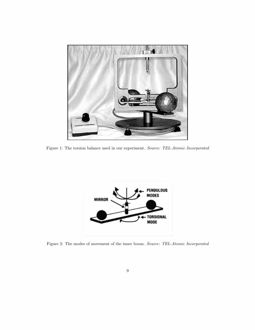
Figure 1: The torsion balance used in our experiment. Source: TEL-Atomic Incorporated

Figure 2: The modes of movement of the inner boom. Source: TEL-Atomic Incorporated

9

Vibration

Isolation

Table

10

Convex Lens

Torsion Balance

He−Ne Laser

30.8 cm

45.7 cm

45.7 cm

91.4 cm

Yardstick

61.0 cm 61.0 cm

Figure 3: A schematic diagram of our optical lever arrangement. Our intended beam path isindicated with a dashed line. All measurements were made with a yardstick and are subjectto an error of +/- 0.7 cm (1/4 inch).

10

Figure 4: The positions of the large spheres, with dimensions. Source: PASCO Scientific

Var. Dimension Measurement Uncertainty UnitsBeam spot size 3.8 0.2 mm

∆S Beam displacement 3.2 0.2 mm2 · d Dist. betw. small spheres (OC) 13.3 0.1 cmb Dist. betw. small and large sphere (horizontal, OC) 4.52 0.2 cm

Dist. betw. small and large sphere (radial, OC) 0 0 cmDist. betw. small and large sphere 1.31 0.2 cm(vertical, top surface to top surface)Mass of large sphere 1 917.5 0.1 gMass of large sphere 2 918.3 0.1 gMass of small sphere 3 14.7 0.1 gMass of small sphere 4 14.6 0.1 g

Table 2: Dimensions of the balance used in our experiment. “OC” stands for On Center.

Var. Value Absolute Fractional Unitserror error

A 0.0191787 0.0002067 1.078% Vβ 0.00113951 4.417e-05 3.876% 1

secω1 0.0390873 3.861e-05 0.09878% rad

sect0 82700 0 0 secδ 1.77528 0.009584 0.5399% radC -1.01427 6.119e-05 0.006033% V

Table 3: Parameters of fit in figure 8.

11

Figure 5: The dimensions of our optical lever arrangement, in two positions. Source: PASCO

Scientific

Var. Value Absolute Fractional Unitserror error

A -0.029903 0.0002861 0.9569% Vβ 0.0012693 4.817e-05 3.795% 1

secω1 0.0386047 4.981e-05 0.129% rad

sect0 86350 0 0 secδ 1.22208 0.0102 0.8344% radC -0.98473 9.348e-05 0.009493% V

Table 4: Parameters of fit in figure 9.

12

-1.02

-1.01

-1

-0.99

-0.98

-0.97

-0.96

5 10 15 20

Vol

tage

(V

)

Time (hrs)

Expt. data

Figure 6: A long period of measurement showed the balance’s equilibrium point drifted overtime.

Var. Value Absolute Fractional Unitserror error

A 0.0265612 0.0002192 0.8254% Vβ 0.00113724 3.372e-05 2.965% 1

secω1 0.0389085 3.087e-05 0.07933% rad

sect0 89730 0 0 secδ 1.84155 0.007355 0.3994% radC -1.01772 6.546e-05 0.006433% V

Table 5: Parameters of fit in figure 10.

Var. Dimension Measurement Uncertainty UnitsDiameter of large sphere 5.46 0.03 cm

2 · r Diameter of small sphere 1.36 0.01 cmml Mass of large sphere 917.9 0.1 gms Mass of small sphere 14.7 0.1 g

Angular frequency of oscillation 2.3320 0.0042 radmin

ω0 0.03887 0.00007 radsec

Table 6: Averaged dimensions used to obtain final results.

13

-1.06

-1.04

-1.02

-1

-0.98

-0.96

-0.94

22.5 23 23.5 24 24.5 25 25.5 26

Vol

tage

(V

)

Time (hrs)

Expt. data

Figure 7: Measurements used to obtain our final result.

Dimension ValueσS 1.795893 ·10−22

σb 3.600506 ·10−22

σd 1.022378 ·10−23

σr 1.724830 ·10−28

σω 1.487970 ·10−25

σm 1.363877 ·10−28

σL 5.871128 ·10−25

σG 2.346487 ·10−11

Table 7: Differential and final error calculations, for comparison.

14

-1.035

-1.03

-1.025

-1.02

-1.015

-1.01

-1.005

-1

-0.995

82700 82800 82900 83000 83100 83200

Vol

tage

(V

)

Time (sec)

Expt. dataFit eqn.

Figure 8: Measurements used to obtain our final result, with fitted equation (see text).

15

-1.02

-1.01

-1

-0.99

-0.98

-0.97

-0.96

-0.95

86350 86400 86450 86500 86550 86600 86650 86700 86750

Vol

tage

(V

)

Time (sec)

Expt. dataFit eqn.

Figure 9: Measurements used to obtain our final result, with fitted equation.

16

-1.045

-1.04

-1.035

-1.03

-1.025

-1.02

-1.015

-1.01

-1.005

-1

-0.995

-0.99

89750 89800 89850 89900 89950 90000 90050 90100 90150 90200

Vol

tage

(V

)

Time (sec)

Expt. dataFit eqn.

Figure 10: Measurements used to obtain our final result, with fitted equation.

17

Acknowledgments

This experiment can be likened (in more ways than one) to a journey into outer space. Itwas by the work of John Wray and myself, alone, that our mission was accomplished. Assuch, I would like to acknowledge ourselves for a dedicated and inspired effort. I would alsolike to acknowledge our patience that was quickly burnt up in the process of rethreadingthe torsion balance. I take my hat off to those who tie fishing flies.

References

[1] Clarendon Laboratory Archive, History of Boys’ experiment, Retrieved Nov. 09, 2004from http://www1.physics.ox.ac.uk/History/BigGHistory.html

[2] Halliday, D., Resnick, R., and Walker, J., Fundamentals of Physics, 6th ed. (2001) NewYork: John Wiley and Sons, Inc.

[3] PASCO Scientific, “012-06802B Gravitational Torsion Balance” manual. (1998) Ro-seville, CA.

[4] Saeta, P., The Cavendish Experiment, Retrieved Nov. 09, 2004 fromhttp://kossi.physics.hmc.edu/Courses/p23a/Experiments/Cavendish.html

[5] TEL-Atomic, Incorporated, “TEL-RP2111 Computerized Cavendish Balance” manual.(1994) Jackson, MI.

[6] Thornton, S. and Marrion, J., Classical Dynamics of Particles and Systems, 5th ed.(2004) Belmont, CA: Brooks / Cole.

18