Embed Size (px)
Citation preview

Measuring the Efficiency of Construction Companies Measuring the Efficiency of Construction Companies Measuring the Efficiency of Construction Companies Measuring the Efficiency of Construction Companies in Gaza Stripin Gaza Stripin Gaza Stripin Gaza Strip
Using Data Envelopment Analysis DEAUsing Data Envelopment Analysis DEAUsing Data Envelopment Analysis DEAUsing Data Envelopment Analysis DEA
Prepared by
Younis M. Shoman
Supervised by:
Dr. Salah R. Agha
Department of Industrial Engineering
&
Dr. Jihad T. Hamed
Department of Civil Engineering
A Thesis Submitted in Partial Fulfillment of Requirements for the
Degree of Master of Science in Construction Management
The Islamic University of Gaza- Palestine
March 2009
The Islamic University of Gaza
Higher Studies Deanery
Faculty of Engineering
Civil Engineering/ C.M
غــزة–الجـامعة اإلسـالميـة
اـعمادة الدراسـات العلي
كليـــة الهندســــة
إدارة التشييد / الهندسة المدنية

i
بسم اهللا الرحمن الرحيم
و���� أن ����� �� ا����� "
��ا �� ا��رض ��ا �
!"��و�#��"! أ&��% و�#
"ا��ار)'� صدق اهللا العظيم

ii
Dedication To my mother "may God have mercy on her soul" for her continuous prayers.
To my father "may God keep for long life".
To my wife for her continuous encouragement, sacrifice.
To my sons and daughters, the hope.

iii
ACKNOWLEDGMENT
All praise and thanks are due to Almighty Allah, Most Gracious; Most Merciful, for the
immense mercy which have resulted in accomplishing this research. May peace and
blessings be upon prophet Muhammad (PBUH), his family and his companions.
I would like to express my deep gratitude to Dr. Salah Agha and Dr. Jihad Hamed for
their continued guidance, supervision and comments during this study. I wish to
acknowledge president of Islamic university of Gaza Dr. Kamalain Sha'at for his
sensible efforts in the presidency of the university and in the construction management
department as a lecturer.
Finally, My extreme appreciation to Ministry of housing and public works, Palestinian
contracting union, national classification committee, and contractors, whom I included
in this study, for their cooperation and support.

iv
Abstract
The science of performance measurement has rapidly developed towards the end of the
last century with the emergence of Data Envelopment Analysis (DEA) technique. This
powerful technique has contributed considerably to solve the problem of measuring the
performance of organizations called Decision Making Units (DMUs) with multiple
inputs and outputs. DEA model is a linear programming-based technique for measuring
the relative efficiency of DMUs. The initial study focused on identifying the measures
(variables) of efficiency and identifying vital measures (variables) of input and output.
These input and output variables are determined through a questionnaire survey for
construction companies of the first grade working in the fields of buildings, roads,
water and sewage, and electromechanical works. The annual average of materials cost,
labor cost, cash flow, subcontractors cost, equipment and machine value, and the
number of management staff are used as input variables. The average annual amount of
executed works is used as the single output variables. Determining input and output
variables facilitated formulating the basic DEA model.
In this research, the mathematical background and characteristics of DEA model is
presented and a short case study on construction companies work in Gaza Strip through
the period from 2002 to 2006 is given. Input oriented DEA model was used under the
assumptions of constant returns to scale and variable returns to scale to evaluate the
relative efficiency of 22 of the leading construction companies.
The study revealed that there is no technique used to measure the efficiency of
construction companies in Gaza. The overall technical efficiency, technical efficiency,
and scale efficiency were investigated by Efficiency Measurement System program
(EMS). The efficiency analysis not only provides an efficiency score for each DMU but
also how much and in what areas an inefficient DMU needs to be improved in order to
be efficient. Inefficient companies have to reduce their resources where they suffer of
intensive possessed machines, cash flow, and management staff. Efficiency analysis
found that construction companies have high efficiency scores. The average technical
efficiency growth trend over time was 1.27%. It was found that the overall technical
efficiency average scores was 94.4%, technical efficiency average score was 98.9%,
and the scale efficiency was 95.2%.

v
� ا�����
��ء ����� �� �� ا���ن ا���� �� ��� � ���� س ا�داء �� � ت �!�ر ��#� ��#+ ا�'���#� ا�'#� . ا�'(��) ا�'&��%� ��$�
س أداء ا���,�## ت ##��ا��'=##1دة ) ا�'##� �!�##: ����## و0##1ات �##8 �� ا��##�ار(##6 ه�4 إ�##2 0##1 آ$�##� �##� ##0) /## آ)
تإن ����� ا�'(��) ا� . ا��A1@ت وا��?�< ت � ءة ا��#�$�� '&��%� ��$�#%Bس ا� أ6��ب /$�� ��2 ا�$�/C#� ا�?!�#� ���#
��1 رآEت ا�1را�6 /$��1 . ��10ات �8 �� ا���ار F�� ءة وآ#�G+ �(�1#1 ا��'&�#�ات ) /'&�#�ات ( ��1�1)� 2 /�##%Bا�
�#2 ا�= /�#� �#� �#�آ ت ا�'#��J#/ 1 ا�1ر<#� ا�و ) ا#6'$ �K (ا�6 � ��6��A1@ت وا��?�< ت /A J@ل /�H /�#1ا��
+#�� B�/و��Bل ا� ري، وأ��##Cوا�� N ل ا����، وا�!�ق، وا���#C/ . �و� ا��#�اد، وا�=� �#�، وا�#����� ا����1#�، و/�#
� ت، وا�!��Pوا��=1ات وا ،JQ ا#6'?4/1 ���#� ا���# ل ا���%#Gة �ا�$��� اRداري ا6'?4/1 آ�'&��ات ���A1@ت
'&��ات ا��A1@ت وا��?�<# ت /�#1ت ا�!��#: ���#U 8#�&� ��#�ذج ا�'(��#) إن �(1�1 / . آ�'&�� و1�0 ���?�< ت
ت� .ا�'&��%� ��$�
ت وآ#�G+ درا�#6 0 �#� �#�آ ت #� �1� �$Gة ر� ��� و/�Eات أ6��ب ا�'(��) ا�'&��%#� ��$��� �� V)$ا ا�Gل ه@A J/
�J ا���ام �=� ع EXة �� ا�%'�ة ا��ا!�'�<�K ا��A1�� J/ أ6#��ب ا�'(��#) ��^ ا�. ٢٠٠٦ -�٢٠٠٢��1 �=�) ��
ءة ا��#�$�� %Bد /`_�ات ا� Cإ� �� �C)�� وا�=�ا�1 ا��'&��ة �C)�� �' aس ا�=�ا�1 ا� ��� K/ا6'?1ا � ت �� ا�'&��%� ��$�
.�=1د اJ��b و���J _�آ� /J _�آ ت ا�'��1 ا��ا�1ة
ع E#Xة أ��cت ا�1را�6 �1م و<�د أي �Qق /'$=� ��� س آ% ءة _�آ ت ا�'��1 !� ءة ا�%��#� . �� #%Bد ا� #Cإ� �#� 1#��
d#6�)ءة ا�� #%Bس ا� �� م ,� e/ �� 6'?1ام ���C)ءة ا� %Bءة ا�%��� ا�$('�، وا� %Bوا� ،���Bا� . f ءة #%B#) ا���إن �(
ل ا�'(���C/1ار و�/ ( ءة ��10ة �8 �� ا���ار %B^ /�1ار ا��� �ت�=!�X 10ة��آ%#�ءة � � H$g#'� ءة�#%Bا� . +#��
�� /##J ز�# دة #0 دة �##� ا��=#1ات وا�#����� ا����##�1 #=� V#�0 ���#�i /�ارده###���� d##>�'� ءة�#%Bا� �#�X ت ا�#�آ
J�#دار�Rوا . �#�� �=f1#ت آ%## ءة � U##'�'� 1��##'ت ا� ءة أن _#�آ##%B##) ا���4 �(#$bوأ دة �##� . آ�####�E1ل ا�#=/ j##� 1##�و
ءة ا�%��� �$� ��6ا %B١ ا�1را�6 تا�l1ا %. ٢٧�/ j� ءة ا�%��#� آ� و%B٩٤ر /'�6^ در<� ا�l٤% ^#6�'/ و/�#1ار ،
ءة ا�%��� ا�$('� %B٩٨ا�l٩% ���C)ءة ا� %B1ار /'�6^ ا��/ j� J�0 �� ،٩٥l٢.%

vi
Table of Contents Dedication ………………………………………………………………. ii
Acknowledgement ………………………………………………………… iii
Abstract ……………………………………………………………………. iv
Arabic Abstract (V)$ا� i?�/) ……………………………………………… v
Table of Contents ………………………………………………………….. vi
List of Acronyms ………………………………………………………….. ix
List of Tables ……………………………………………………………… x
List of Figures ……………………………………………………………... xi
Chapter 1: Introduction 1
1.1 The Importance of Construction Industry ……………………………... 2
1.2 Construction Industry in Gaza ………………………………………… 3
1.3 Construction Industry Effect on Economy …………………………….. 3
1.4 Motivation ……………………………………………………………... 3
1.5 Scope and Limitations …………………………………………………. 4
1.6 The Importance of the Study …………………………………………... 4
1.7 Research Questions ……………………………………………………. 4
1.8 Aim of the Study ………………………………………………………. 5
1.9 Objectives ……………………………………………………………… 5
1.10 Organization of the Thesis …………………………………………… 5
Chapter 2: Literature Review 6
2.1 Importance of Performance Measurement …………………………….. 6
2.2 Measurement Techniques ……………………………………………... 8
2.2.1 Basic Models of DEA ……………………………………………. 11
2.2.2 Returns to Scale ………………………………………………... 19
2.2.3 Scale Efficiency …………………………………………………. 20
2.2.4 Comparison of SFA and DEA Methods ……………………….... 21
2.3 Efficiency ……………………………………………………………… 23
2.3.1 Definition of Efficiency …………………………………………. 23
2.3.2 Categorization of Efficiency …………………………………….. 24

vii
2.3.3 Productivity ……………………………………………………… 25
2.3.4 Efficiency Measurement in Construction Sector ………………… 26
2.3.5 Efficiency Measures in Construction Industry ………………….. 28
Chapter 3: Methodology 31
3.1 Research Design ………………………………………………………... 31
3.2 Research Location and Period …………………………………………. 31
3.3 Experts Opinion Investigation ………………………………………… 31
3.3.1 Contractors Opinion ………..........………………………………. 31
3.3.2 Participants Opinion ..……………………………………………. 33
3.4 Description of Data ……………………………………………………. 33
3.4.1 Input Measures (Variables) ……………………………………… 35
3.5 Research Population …………………………………………………… 36
3.6 Sample Size Determination ……………………………………………. 37
3.7 Data collection …………………………………………………….. 38
3.7.1 Questionnaire Design and Contents ……………………………... 38
3.7.2 Pilot Study ……………………………………………………….. 40
3.7.3 Instrument Validity of the Questionnaire by Arbitrators ………... 40
3.7.4 Instrument Validity by Pilot Study ……………………………… 40
3.7.5 Instrument Reliability …………………………………………… 41
3.8 Case Study ……………………………………………………………... 41
3.8.1 Case Study Forms ……………………………………………….. 41
3.8.2 Forms Validity …………………………………………………... 43
3.8.3 Participant Companies …………………………………………... 44
3.8.4 Distribution of Case Study Forms ………………………………. 45
3.8.5 Case Study Limitations ………………………………………… 45
3.9 Method of Data Analysis ……………………………………………… 46
Chapter 4: Results and Analysis 48
4.1 Field Survey Statistical Results ……………………………………….. 48
4.1.1 Respondents Characteristics …………………………………….. 48
4.1.2 Determining the Vital Measures of Efficiency ………………….. 48
4.2 Selected Variables ……………………………………………………... 54

viii
4.2.1 Description of Variables ………………………………………… 55
4.3 Model Building ………………………………………………………... 57
4.4 Case Study Data ….……………………………………………………. 59
4.5 Case Study Results …………………………………………………….. 66
4.5.1 Sample Characteristics …...……………………………………… 66
4.5.2 Results and Analysis ………………………………………….…. 67
4.5.3 Trends of Technical Efficiency Scores over Time ………………. 79
4.5.4 Trends of Input Usage over Time ………………...……………... 81
4.5.5 Characteristics of Efficient and Inefficient DMUs ………………. 82
4.5.6 Performance Measurement Tools ……………………………….. 88
4.5.7 DMUs Ranking ………………………………………………….. 88
4.5.8 Relationship Between Executed Works and Efficiency ……….. 90
Chapter 5: Conclusion and Recommendation 91
5.1 Conclusion …………………………………………………………….. 91
5.2 Recommendation ……………………………………………………… 93
References 96
Appendixes i
Appendix 1 ………………………………………………………………... ii
Appendix 1-A …………………………………...……………………… ii
Appendix 1-B …………………………………………...……………… v
Appendix 1-C …………………...……………………………………… viii
Appendix 2 ………………………………………………………………... xxiii
Appendix 2-A ………...………………………………………………… xxiii
Appendix 2-B ……………………...…………………………………… xxvii
Appendix 3 ………………………………………………………………... xxxi
Appendix 3-A …………………………...……………………………… xxxi
Appendix 3-B ………………………………...………………………… xxxii
Appendix 3-C ………………………………………...………………… xxxv
Appendix 3-D ………………………………………………...………… xxxviii

ix
List of Acronyms and Abbreviations BCC Banker, Charnes, Cooper Model.
CCR Charnes, Cooper, Rhodes Model.
CF Cash Flow
CRS Constant Returns to Scale.
DEA Data Envelopment Analysis.
DMU Decision Making Unit.
DMUs Decision Making Units.
EM Equipments and Machines
EMS Efficiency Measurement System.
EW Executed Works.
GDP Gross Domestic Product.
L Labor.
M Used Materials.
MPW&H Ministry of Public Works and Housing.
MS Management Staff.
PCU Palestinian Contractor Union.
PNA Palestinian National Authority.
SPSS Statistical Package for the Social Sciences.
SUB Subcontractors.
VRS Variable Returns to Scale.

x
List of Tables Table 2.1 Comparison between SFA and DEA 22
Table 2.2 Efficiency Variables 30
Table 3.1a Input Variables Classified According to Data Source 34
Table 3.1b Output Variables Classified According to Data Source 35
Table 3.2 The population study 36
Table 3.3 Likert Scale of Evaluation 39
Table 3.4 Summary of the Averages of collected variables (2002-2006) 44
Table 3.5 Invited Construction Companies 46
Table 4.1a Average Weights of Inputs Variables 50
Table 4.1b Average Weights of Output Variables 50
Table 4.2a Statistical Analysis of the Input Variables 52
Table 4.2b Statistical Analysis of the Output Variables 52
Table 4.3a Values of Input and Output Variables in Year (2002) 60
Table 4.3b Values of Input and Output Variables in Year (2003) 61
Table 4.3c Values of Input and Output Variables in Year (2004) 62
Table 4.3d Values of Input and Output Variables in Year (2005) 63
Table 4.3e Values of Input and Output Variables in Year (2006) 64
Table 4.4 Summary of the Averages of the Variables Values (2002-2006) 65
Table 4.5 Statistical Results of the Input and Output Variables 66
Table 4.6 Fields Contribution to Executed Works 67
Table 4.7 DMUs Overall Technical Efficiency (CCR) Scores over Time 69
Table 4.8 DMUs Technical Efficiency (BCC) Scores over Time 70
Table 4.9 DMUs Scale Efficiency Scores over Time 71
Table 4.10 Benchmarks of Inefficient Companies in 2006 73
Table 4.11 Target Improvements of Inefficient DMUs in CCR Model 74
Table 4.12 CCR Potential Improvements Percentage of Inefficient DMUs 74
Table 4.13 Summary of Improvement Percentage of CCR Model 79
Table 4.14 Summary of Annual Variables Weights over the Study Period 81
Table 4.15 Categories of Efficient and Inefficient DMUs and Their
Percentages
84
Table 4.16 Efficiency Scores and Ranks for DMUs over Time 89
Table 4.17 Efficiency Scores and Annually Ranks for DMUs over Time 90

xi
List of Figures Figure 1.1 Graphical Representation of the DMU 2
Figure 2.1 CCR Production Possibility Set and Frontier 12
Figure 2.2 Envelopment Surface and Projections in CCR-I Model 14
Figure 2.3 Envelopment Surface and Projections in CCR-O Model 16
Figure 2.4 Envelopment Surface and Projections in the BCC-I Model 17
Figure 2.5 Envelopment Surface and Projections in the BCC-O Model 19
Figure 2.6 Returns to Scale 20
Figure 2.7 Technical and Scale Efficiency 21
Figure 3.1 Research Methodology Flowchart 32
Figure 4.1 Characteristic of Respondents 49
Figure 4.2a Input Variables Scree Plot 53
Figure 4.2b Output Variables Scree Plot 53
Figure 4.3 Output's Components of executed works 67
Figure 4.4 EMS Outputs 68
Figure 4.5 CCR Improvement Percentages of C4 75
Figure 4.6 CCR Improvement Percentages of C9 76
Figure 4.7 CCR Improvement Percentages of C11 76
Figure 4.8 CCR Improvement Percentages of C13 77
Figure 4.9 CCR Improvement Percentages of C21 77
Figure 4.10 CCR Improvement Percentages of C22 78
Figure 4.11 CCR Potential Improvements Percentages of Inefficient DMUs 79
Figure 4.12 Number of Efficient DMUs over the Study Period 80
Figure 4.13 Trends of Average Technical Efficiency of DMUs over Time 80
Figure 4.14 Trends of DMUs Usage of Inputs over Time 82

1
Chapter 1
Introduction
The construction industry has played a vital role in developing and developed countries. It
is the major contributor to the gross domestic product (GDP) in Palestine (West Bank and
Gaza Strip), where it contributes 33% to the Palestinian GDP and it is the largest
employer of the work force. It reached up to 22.3% in 1999 (PCU, 2008). It is the most
significant player in the economy of Palestine. Construction industry includes
construction companies that perform a number of different projects dispersed into various
and divergent sites, where the physical production is performed. This production is not
always performed as planned due to realistic surrounding circumstances. Projects are
unique in nature and the construction process varies widely due to variations in materials,
machines, quality, safety, location, construction staff, subcontractors, and others can be
changed partially or entirely.
Performance measurement is necessary for continuous improvement to avoid
shortcomings and failures, which create the company's efficiency. Efficiency may be
defined as the ability of a firm to produce as much output as possible, given a certain
level of inputs and certain technology (Nguyen and Giang, 2005). Efficiency requires that
several inputs lead to outputs, which represent the amount of success achieved. Inputs and
outputs are denoted efficiency measures, and sometimes variables.
Construction industry nowadays suffers from hyper competitiveness. Sustainable
competitive advantage is built by firms only through efficiency and effectiveness.
Efficient companies mean success to all construction players. So, firms having sufficient
power with qualified and superior resources are able to perform more efficiently. Main
parties of construction industry; client, designer, and contractor may pay no attention to
efficiency which affect all parties. So, companies are under stress to find ways to improve
their performance to survive and sustain their competitive position in the local
construction market. Performance measurement is a critical component of the
management process in any type of organization. Measuring relative efficiency of
Decision-Making Units (DMUs) with incommensurate inputs and outputs has been
problematic for researchers and practitioners. A special linear programming-based model
known as Data Envelopment Analysis (DEA) is capable of addressing such a problem

2
(Al-Shammari, 1999). Fig. 1.1 shows a construction company called Decision Making
Unit (DMU) that uses multiple inputs to produce multiple outputs.
Fig. 1.1 A Graphical Representation of the DMU
So, measuring the efficiency of construction companies is necessary to check and monitor
performance, to verify changes and implications of improvement actions in order to make
effective decisions. As a result, decision of company's selection made by the client, has to
be based not only on the principle of cost, but also based on other criteria such as; on-time
delivery, quality, available resources, superiority, creativeness, safety, client or end-user
satisfaction, and friendliness to environment. Efficiency, simply may be defined as the
optimal consumption/use of available resource-s (input-s) to produce the largest amount
of valuable benefit-s (output-s).
1.1 The Importance of Construction Industry
Construction industry is a corner stone for most nations industries. All over the world, no
urban progress is made without construction. It is the underpinning of both manufacturing
and services industry. It is the most developing element in social promotion, and
economic strengthening, but it is burdensome in execution and cost, that it exhausts one-
half of the gross capital and constitutes 3-8% of Gross Domestic Product (GDP) in most
countries (Arditi and Mochtar, 2000).

3
1.2 Construction Industry in Gaza
Gaza Strip is a zone of Palestinian territory. It is a populous and narrow area. Its area is
about 362 square kilometers and its projected population in 2010 is 1.6 millions. Since,
the emersion of the Palestinian National Authority in 1994, the construction sector has
witnessed remarkable activities, which resulted in revival of construction sector, support
industries and emigrant capital investments. Construction industry is one of the most
vibrant industries in Gaza Strip. It includes general contractors, builders, subcontractors,
specialty trades and suppliers. Construction works include activities related to construct
of residential building, schools, offices, roads, bridges, pipelines, airports, harbors,
drainage, power plants, water supply, railways, irrigation projects, maintenance and repair
works.
1.3 Construction Industry Effect on Economy
Construction industry is a vital contributor to the Palestinian economy. It includes the
overall building community and consists of: owners, operators, and users; developers,
designers, contractors, fabricators, manufacturers and suppliers; regulators, codes and
standards organizations, building and fire safety officials, labor, financial organizations,
testing laboratories, educational institutions, and research organizations (Raufaste and
Callahan, 2002).
The construction industry is a powerful engine to the Palestine economy in general and
especially in Gaza Strip. Construction sector supports the Palestinian economy in two
directions. The first one, is its contribution to GDP with 33% which exceeds the average
rate of most countries, and secondly in job creation where it employs about 22.3% of the
local workforce in 1999 before the Israeli redeployment in September 2000 (PCU, 2008).
1.4 Motivation
The main motivation of the study stems from the belief that no studies have estimated
technical efficiency of construction companies in Gaza Strip. A number of studies have
been carried out on construction companies in Gaza Strip, such as causes of contractors'
failure in Gaza Strip (Hallaq, 2003), measurement of labor productivity in Gaza Strip
(Abo Mostafa, 2003), and modeling the factors affecting quality of building construction
projects (Amer, 2002). Cost and time performance are conducted in the context of
individual projects but they do not reflect the efficiency status of the company. Measuring

4
efficiency demonstrates a comprehensive image of company. To the researcher’s
knowledge no studies were conducted to measure efficiency.
1.5 Scope and Limitations
Construction industry has huge scope and hence large amount of resources involvement,
and complexities in managing it. This is the reason that leading construction companies
were selected for this research. Due to time and accessibility constraints, the study was
limited to the Southern provinces (Gaza Strip) of Palestine. This research is performed
based on contractors’ point of view, because the contractor is the main party responsible
for the resources supply and management throughout construction phase of any project.
The measures of inputs and outputs were obtained using literature review, experts
interviews and researcher experience.
1.6 The Importance of the Study
A study took place to investigate the causes of construction industry failure (Hallaq,
2003), but no attention was paid to enable companies to counter unstable conditions,
market variability and resources shortage. Sustainable development has to recruit efficient
companies for improving performance in terms of quality, safety, clients satisfaction,
cost, time, material consumption, strengthening economy, employees recruiting and
minimizing claims, where these terms are the most valuables. So, it is necessary to find an
instrument to measure construction companies efficiency.
1.7 Research Questions
1- Do agencies apply any tools to measure the efficiency of construction companies? If
yes, what are they?
2- What are the main inputs of construction companies?
3- What are the main outputs of construction companies?
4- Is there a relationship between efficiency and profitability?
5- What are the characteristics of efficient companies?
6- What are the characteristics of inefficient companies?

5
1.8 Aim of the Study
To study the efficiency of construction companies in the local market using data
envelopment analysis (DEA). The study will identify the role of inputs and outputs in
determining the efficiency of construction company. Then, the companies will be ranked
according to their efficiency. Recommendations for improvements given to inefficient
companies.
1.9 Objectives
The study will address the following objectives:
1- To investigate the measures of efficiency; technical, financial, managerial, and others.
2- To investigate and identify the main measures of inputs of construction companies.
3- To investigate and identify the main measures of outputs of construction companies.
4- To identify the common characteristics of efficient companies.
5- To identify the common characteristics of inefficient companies.
6- To establish a compact efficient company model using data envelopment analysis
DEA.
1.10 Organization of the thesis
This thesis is organized into five chapters: Chapter 1 introduces the problem to be
addressed and the research objectives for this thesis. This chapter also includes general
information of research and the structure of the thesis.
Chapter 2 provides background introduction of performance measurement and DEA, also
some recent studies on efficiency topic and applications of DEA. Chapter 3 includes the
research methodology. It explains the procedure of finding the measures of efficiency and
how DEA is applied to calculate the efficiency in this research. Results and discussion are
given in Chapter 4. Finally chapter 5 summarizes the conclusion and recommendation of
the study.

6
Chapter 2
Literature Review
To evaluate performance, it must be measured. Performance measurement is the key to
progress in any organization. In order to be competitive, improving efficiency is an
important issue. Efficiency is one of the most issues for many nations. It is the key
measure of utilization of available resources (inputs) to convert them into meaningful
physical products (outputs). This chapter is divided into three sections; the first one
provides an overall look of the importance of performance measurement, the second
section provides a background of measurement techniques of both parametric and non-
parametric approaches, where the third section discusses the current issues related to
efficiency; definition, categorization, its measurement and measures in construction
industry.
The construction industry has been practicing construction for the last 4,000 years.
Industries have proven that performance measurement is the cornerstone of challenging
any industry to become world class (Alarcon et al., 2008). Performance measurement has
been given a prominent place in most organizations that are called Decision Making Units
(DMUs) as it helps to achieve continuous improvements (Martinez, 2005; Baldwin et al.,
2001). Performance measurement is defined as “the process of determining how
successful organizations or individuals (DMUs) have been in attaining their objectives
and strategies” (Kagioglou et al., 2001). Cain, 2004 and Alarcon et al., 2008, identifies
performance measurement as the first stage of any improvement process that benefits the
end users with lower prices and the organizations with higher profit margins, whilst
enhancing the quality of the product. A wider definition of performance measurement
systems is given by Neely (1998) as the quantification of efficiency and effectiveness of
past actions by means of data acquiring, collection, sorting, analyzing, interpreting and
disseminating.
2.1 Importance of Performance Measurement
The gap in construction industry is the lack of performance measurement methodology
that likely retards industrial adoption of new methods and cost excesses. In USA labor
cost excesses between 30%-40% due to the losses of productive time in the industrial
construction projects caused mainly by the inefficiency work process and other factors
(Picard, 2000). The Australian construction industry has been portrayed as being

7
uncompetitive and inefficient. The Australian construction industry claiming that: “…up
to 40% of effort in developing and operating capital works facilities is wasted and adds
no value to the end user/customer whilst depleting profitability of the client, designers
and contractors” (Gallo, et al., 2002).
(Love and Holt, 2000) summarize the importance of performance measurement as:
• Ensuring that customer requirements are properly met (and if not, why);
• Enabling the organization of achievable business objectives and monitoring
compliance;
• Providing standards for business comparisons;
• Providing transparency and a scoreboard for individuals to monitor their own
performance;
• Identifying quality problems and those requiring priority attention;
• Giving an indication of the costs of poor quality;
• Justifying the use of resources;
• Providing feedback for driving the improvement effort; and
• Regularly measurement sets competitive environment between organizations
(DMUs) to compare their own products, services and business processes against
the best within or outside their industry – seeking to unearth and implement best
practice from whatever source.
Performance measurement is an important aspect for organizations to evaluate their actual
objectives against predefined goals and to make sure that the organization is doing well in
the competitive environment. Nevertheless, performance measurement is not without any
disadvantages. Performance measurement enables managers to make decisions based on
facts rather than on assumptions and faith (Parker, 2000). Therefore performance
measurement has become an integral part of planning and controlling organizations.
For competitive construction industry, there is a critical need for management actions to
continuously improve the firm's performance. In the long term, success of both individual
construction firms and the industry overall will depend on improving performance by
continually acquiring and applying new knowledge. Measurement aims at comparing the
performance of firms relative to each other, allowing these firms to recognize their
weaknesses and strengths compared to the industry. Measurement aids in the
identification of industry leaders who exhibit superior performance as a result of using
best industry practices. By finding examples of superior performance, firms can adjust

8
their policies and practices to improve their own performance and become more similar to
performance leaders in the industry (EL-Mashaleh et al., 2007). Performance
measurement assists managers in staff allocation based on activities' level and determines
where excess resources are being utilized.
Efficiency measurement has a bundle of managerial advantages as:
• Supports management decisions to maximize resource utilization across projects
for achieving the highest level of return.
• Supports management decisions about investment in resources and in mix of
projects.
• Supports concept of benchmarking, that allowing contractors to better understand
their competitive position and improve their performance.
• Supports comparative research of various management policies.
• Determines the actions that should or could be made in the short term to improve
performance,
• Identifies the strong and weak areas within the company, and
• Helps the construction industry to learn as a whole (El-Mashaleh et al., 2001 and
Alarcon et al., 2008).
2.2 Measurement Techniques
Efficiency measurement technique has been given a prominent place in most
organizations (DMUs) as it helps to achieve continuous improvements. Farrell (1957) laid
the foundation to measure efficiency studies at the micro level. The estimation of
efficiency can be categorized according to the assumptions and techniques used to
construct the efficient frontier. Parametric methods estimate the frontier with statistical
methods. On the other hand, nonparametric methods rely on linear programming to
calculate linear segments of the efficient frontier. These two methods are discussed
below.
The parametric frontier approach specifies a functional form for the cost, profit, or
production relationship among inputs, outputs, and environmental factors, and allows for
random error. The most used technique is Stochastic Frontier Analysis (SFA), which is a
parametric method and is based on the quantitative economy theory. Parametric method is
based on parameter estimation with given functional forms (in practice, it is impossible to
apply one technology for all different industries, or even to do so for all firms within an

9
industry). Thus, identifying an appropriate technology for each industry or firm is also
difficult. Researchers find out that parametric approaches are best applied to industries
with well-defined technologies to minimize the risk of misspecification.
Unlike the parametric approach, which is based on functional forms without linear
programming, the non-parametric method is based on linear programming without
functional forms of the frontier nor any distributional assumptions. In this section, Data
Envelopment Analysis (DEA) will be discussed in some detail.
Charnes et al. (1978) originally introduced data envelopment analysis (DEA) as a method
to measure relative efficiency of different decision making units (DMUs) or producers
based on their observed inputs and outputs. Their work builds on the same introduced
paper by Farrell (1957) and extends the engineering ratio approach to efficiency
measurement for multiple input–output combinations. The most efficient producers have
relative efficiency of 1 and others have figures between 0 and 1. Data envelopment
analysis (DEA) is commonly used to evaluate the efficiency of a group of producers
(DMUs) such profit or nonprofit organizations, firms, institutions, departments or
operating units. Throughout this research and consistent with DEA terminology, the term
“decision-making unit” or “DMU” will refer to the individuals in the evaluation group. In
the context of this application, it will refer specifically to construction
companies/contractors.
A typical statistical approach evaluates producers relative to an average producer. In
contrast, DEA is an extreme point method which compares each producer with only the
“best” producers. A fundamental assumption behind an extreme point method is that if a
given producer A, is capable of producing Y(A) units of output with X(A) inputs, then
other producers should also be able to do the same if they were to operate efficiently.
Similarly, if producer B, is capable of producing Y(B) units of output with X(B) inputs,
then other producers should also be capable of the same production schedule. Producers
A, B, and others can then be combined to form a composite producer with composite
inputs and composite outputs. Since this composite producer does not necessarily exist, it
is sometimes called a virtual producer. The heart of the DEA technique lies in finding the
“best” virtual producer for each real producer. If the virtual producer is better than the
original producer by either making more output with the same input or making the same
output with less input then the original producer is inefficient. Some of the subtleties of
10
DEA are introduced in the various ways that producers A and B can be scaled up or down
and combined.
As mentioned, the DEA approach has recently become the dominant approach to measure
the performance of many economic sectors. However, when we consider DMUs, we
generally do not know what the optimum efficiency is and therefore we can not determine
whether a DMU is absolutely efficient. DEA enables us to compare several institution
units with each other and determine their relative efficiencies (Sowlati, 2001). Some key
advantages of DEA are summarized as follows:
• It is used to measure the efficiency of homogenous units called decision making
units (DMUs), which consume the same type of inputs to produce the same type
of outputs.
• DMUs are directly compared against a peer or combination of peers. This means
that any inefficient DMU has a reference set display the level of reduction inputs
or the level of increasing outputs to become an efficient unit.
• Inputs and outputs can have very different units. For example, inputs X1 could be
in units of headcounts, X2 could be dollars value, where outputs Y1 could be in
units of square meter, Y2 could be in units of cubic meter and so on.
• DEA reveals the amount of inputs' savings and the amount of outputs' increments
can be achieved by DMU to improve its efficiency.
• It is a nonparametric approach; hence, there is no restriction on the functional
form that relates inputs to outputs.
• It is a fractional mathematical programming technique. However, it can be
converted into a linear programming model and solved by a standard LP solver.
• It generalizes the concept of the single-input, single-output technical efficiency
measure developed by Farrell (1957) to the multiple-input and multiple-output
case by computing a relative efficiency score as a ratio of a virtual output to a
virtual input. Specifically, efficiency is defined as a ratio of a weighted sum of
outputs to a weighted sum of inputs.
• It is an approach that is focused on frontiers instead of central tendencies. It
evaluates the efficiency of each DMU relative to similar DMUs. Thus, it provides
an efficient frontier or envelope for all considered DMUs rather than fitting a
regression plane through the center of the data.

11
• It determines the relative efficiency of one DMU at a time over all other DMUs by
finding the most favorable weights from the viewpoint of that, "target", DMU.
(Lertworasirikul, 2002 and Sowlati, 2001).
The same features that make DEA a powerful tool can also create problems. The
following limitations must be considered when choosing whether or not to use DEA
• Since DEA is an extreme point technique, noise (even symmetrical noise with
zero mean) such as measurement error can cause significant problems.
• DEA is good at estimating “relative” efficiency of a DMU but it converges very
slowly to “absolute” efficiency. In other words, it can tell you how well you are
doing compared to your peers but not compared to a “theoretical maximum”.
• Since DEA is a nonparametric technique, statistical hypothesis tests are difficult
and are the focus of ongoing research.
• Since a standard formulation of DEA creates a separate linear program for each
DMU, large problems can be computationally intensive.
• The DEA method assigns mathematically optimal weights to all inputs and
outputs being considered. It derives the weights empirically, so the maximum
weight is placed on those favorable variables and the minimum weight is placed
on the unfavorable variables (Charnes, 1997, Lertworasirikul, 2002 and Yang,
2005).
2.2.1 Basic Models of DEA
In their original DEA model, Charnes, Cooper and Rhodes (CCR) adopted a ratio for
defining efficiency. It generalizes the single-output to single-input classical engineering
ratio definition to multiple inputs and outputs without requiring preassigned weights.
Inputs of Sum Weighted
Outputs of Sum Weighted=Efficiency (Charnes et al., 1978).
Charnes, Cooper, and Rhodes in 1978 (CCR Model) proposed that the efficiency of any
DMU can be obtained as the maximum of a ratio of weighted outputs to weighted inputs
subject to the condition that similar ratios for every DMU are less than or equal to one.
Using the fractional programming theory, the ratio problem is transformed into an
ordinary linear programming problem (Cooper et. al., 2000). To obtain the efficiency of
all DMUs, it is necessary to solve a series of linear programs, one for each DMU as the
objective function. DEA identifies the most efficient units and indicates the inefficient

12
units in which real efficiency improvement is possible. The amount of resources saving or
services improvement that can be achieved by each inefficient unit to make them efficient
is identified and can be used as indications for management action.
Banker et al., 1984 introduced the BCC model in which the envelopment surface is
variable returns to scale. The CCR model is employed to estimate the overall technical
and scale efficiency of a DMU. However, the BCC model takes into account the
possibility that the most productive scale size may not be attainable for a DMU which is
operating at another scale size. It estimates the pure technical efficiency of a DMU at the
given scale size of operation.
In this section, the focus is on describing the basic DEA models of the CCR, and BCC
models particularly.
CCR Model
This is one of the most basic DEA models, proposed by Charnes et al., 1978. They
introduced the term Decision Making Unit (DMU) to describe the organization under
efficiency study, which can for example be a firm, a department store, or a bank branch,
with common inputs and outputs. A DMU is an entity, which converts inputs to outputs,
and has a certain degree of managerial freedom in decision making.
Input
Out
put
A
D
B
C
F
E
Production Possibility Set
Efficient Frontier
Fig. 2.1 CCR Production Possibility Set and Frontier

13
Figure 2.1 shows the efficient frontier and production possibility set for the CCR model
in two dimensions, the single input and single output case. CCR model mainly has two
possible orientations; CCR input oriented model and CCR output oriented model.
The first type of CCR model is the input oriented model, which tries to minimize the
input usage to produce given output levels for each DMU. Suppose there are n DMUs:
DMU1, DMU2, …, DMUn, with k inputs: kxxx ,...,, 21 and m outputs: myyy ,...,, 21 .
The following fractional programming model can be solved to obtain the efficiency score,
input and output weights.
Min
∑
∑
=
==m
rrr
k
iii
yu
xv
10
10
θ 2.1
Subject to
1
1
1 ≥∑
∑
=
=m
rrjr
k
iiji
yu
xv
For each DMU in sample nj ,...,1= .
Where the following notations are used:
θ is the optimal objective value.
0, ≥ir vu ,
mr ,...,1= ,
ki ,...,1=
Here ijx and rjy (all non-negative) are the inputs and outputs of the thj DMU, iv and ru ,
are the inputs and outputs weights.
The objective is to obtain weights (iv , ru ) that minimizes the efficiency (ratio) of DMU0,
which is the DMU under evaluation. The constraints mean that the efficiency of none of
the DMUs should exceed one, while using the same multipliers.
The above fractional equation 2.1 can be transformed into a linear programming problem
(Charnes et al., 1978).

14
Min ∑=
=k
iii xv
10θ 2.2
Subject to
11
0 =∑=
m
rrr yu
011
≥−∑∑==
m
rrjr
k
iiji yuxv
0, ≥ir vu
For each DMU in sample nj ,...,1=
mr ,...,1= ,
ki ,...,1=
The fractional program equation 2.1 is equivalent to the linear program equation 2.2 and
they have the same optimal objective value, θ . When DMU0, has 1<θ , then it is CCR-
inefficient.
Yet, we have considered a version of the CCR model in which the objective is to
minimize inputs while producing at least the given output levels. This is called the
orientedinput − model. The envelopment surface for the CCR orientedinput − model
(CCR-I) and projections of the inefficient units (B, C and D) to this efficient frontier for
the case of one input and one output are shown in Figure 2.2.
Input
Out
put
A
B
C
D
CCR - I Frontier
CCR - Input Oriented
Fig. 2.2 Envelopment Surface and Projections in CCR-I Model

15
The second type of CCR model is the output oriented model, which aims to maximize
outputs while not exceeding the observed input levels. The fractional form of CCR output
oriented model is as follows:
Max
∑
∑
=
==k
iii
m
rrr
xv
yu
10
10
θ 2.3
Subject to
1
1
1 ≤∑
∑
=
=k
iiji
m
rrjr
xv
yu
For each DMU in sample nj ,...,1=
where the following notations are used:
θ is the optimal objective value.
0, ≥ir vu
mr ,...,1=
ki ,...,1=
Here ijx and rjy (all non-negative) are the inputs and outputs of the thj DMU,
iv and ru , are the inputs and outputs weights.
The objective is to obtain weights (iv , ru ) that maximizes the efficiency (ratio) of
DMU0 (DMU under evaluation). The constraints mean that the efficiency of none of the
DMUs should exceed one, while using the same multipliers.
The above fractional programming model (equation 2.3) can be transformed into a linear
programming problem (Charnes et al., 1978).
Max ∑=
=m
rrr yu
10θ 2.4
Subject to:
11
0 =∑=
k
iii xv
011
≤−∑∑==
k
iiji
m
rrjr xvyu
0, ≥ir vu

16
The fractional program (2.3) is equivalent to the linear program (2.4) and they have the
same optimal objective value, θ . When DMU0, has 1<θ , then it is CCR-inefficient.
Yet, a version of the CCR model in which the objective is to produce the highest possible
output levels for a given input usage is considered. This is called the output-oriented
model. The envelopment surface for the CCR output oriented model and projections of
the inefficient units (B, C and D) to this efficient frontier for the case of one input and one
output are shown in Fig 2.3.
Input
Out
put
A
D
B
C
CCR - O Frontier
CCR - Output Oriented
Fig. 2.3 Envelopment Surface and Projections in CCR-O Model
BCC Model:
The CCR model evaluates both technical and scale efficiency via the optimal value of the
ratio form. The envelopment in CCR is constant returns to scale meaning that a
proportional increase in inputs result in a proportionate increase in outputs.
Banker et al., 1984 developed the BCC model to estimate the pure technical efficiency of
decision making units with reference to the efficient frontier. It identifies whether a DMU
is operating in increasing, decreasing or constant returns to scale. Also, BCC model
mainly has two possible orientations; BCC input oriented model and BCC output oriented
model.
The BCC input oriented model evaluates the efficiency of DMU0, by solving the linear
program given in equation 2.5.

17
Min 01
0 vxvk
iii +=∑
=
θ 2.5
Subject to
11
0 =∑=
m
rrr yu
01
01
≥+−∑∑==
m
rrjr
k
iiji vyuxv
0, ≥ir vu
For each DMU in sample nj ,...,1= .
θ is the optimal objective value.
0, ≥ir vu
mr ,...,1= ,
ki ,...,1= .
free 0v
Figure 2.4 is a two dimensional example that illustrates the envelopment surface and
projections to this frontier. Inefficient units are projected to the efficient frontier by
reducing their input.
Input
Out
put
A
D
B
C
BCC - I Frontier
BCC - Input Oriented
E
F
G
Fig. 2.4 Envelopment Surface and Projections in the BCC-I Model

18
Units A, B, C, D, E are the efficient units and form the efficient frontier. Units F and G
are inefficient. In order to make unit F efficient, a proportional decrease in its input is
needed. For unit G, first a reduction in input level and then an increase in its output is
necessary. If a unit is characterized as efficient in the CCR model, it will also be
characterized as efficient in BCC model, however the opposite is not true.
While the envelopment surface for the BCC output oriented model is the same as BCC
input oriented one, the projection to the envelopment surface in the two models is
different. The objective in BCC output oriented model is to maximize the output
production while not exceeding the actual input level. The linear program for the BCC
output oriented model is given in equation 2.6.
Max ∑=
+=m
rrr uyu
100θ 2.6
Subject to
11
0 =∑=
k
iii xv
0011
≤+−∑∑==
uxvyuk
iiji
m
rrjr
0, ≥ir vu
For each DMU in sample nj ,...,1= .
mr ,...,1= ,
ki ,...,1= .
free 0u
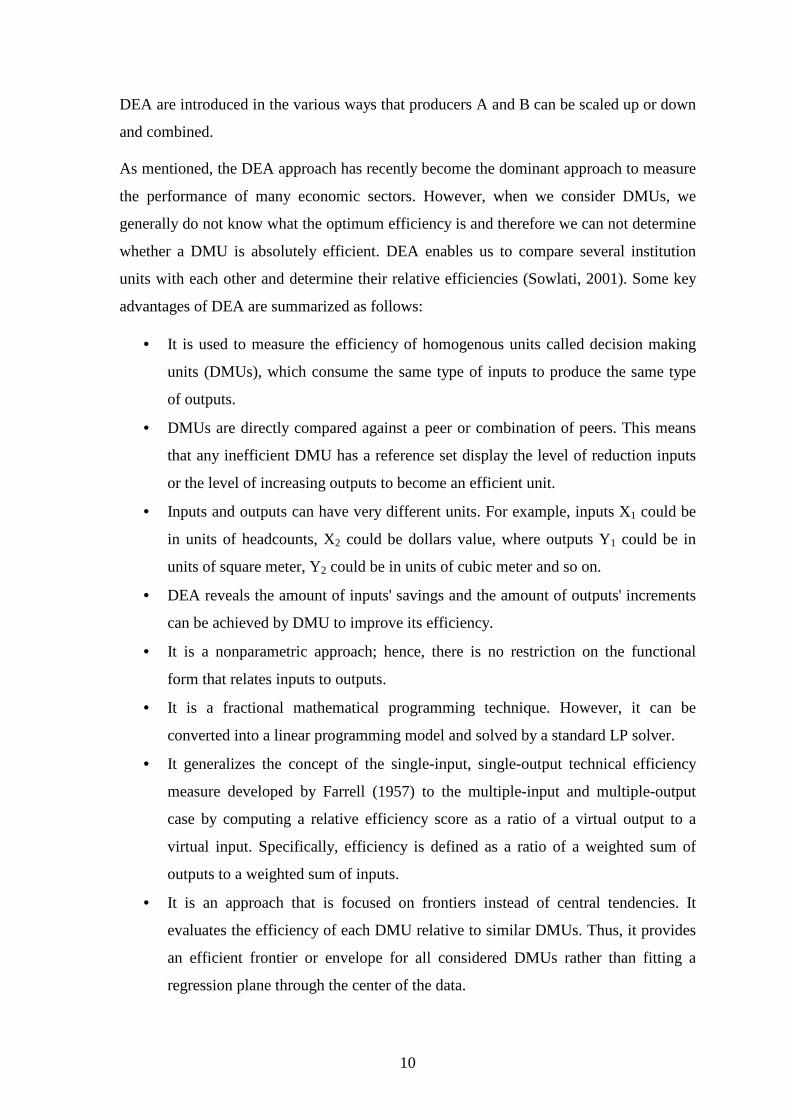
Figure 2.5 is a two dimensional example that illustrates the envelopment surface and
projections to this frontier. Inefficient units are projected to the efficient frontier by
increasing their output.
Units A, B, C, D, E are the efficient units and form the efficient frontier. Units F and G
are inefficient. In order to make unit F and G efficient, a proportional increase in their
outputs is needed. If a unit is characterized as efficient in the CCR model, it will also be
characterized as efficient in BCC model, however the opposite is not true.
Noticeable, there are other broadcast models; additive and multiplicative models are out
of the question and impertinent.
19
Input
Out
put
A
D
B
C
BCC - O Frontier
BCC - Output Oriented
E
F
G
Fig 2.5 Envelopment Surface and Projections in the BCC-O Model
2.2.2 Returns to Scale
In DEA literature, the CCR model is derived based on the assumption of constant returns
to scale of DMUs. For the long-run analysis, the scale of firm's operations should be
considered. The amount of increased outputs associated with increased inputs is
fundamental to the long run nature of the firm's production process. The concept of
returns to scale is addressed in terms of constant and variable returns to scale. The two
types of returns to scale are discussed hereinbelow:
Constant Returns To Scale (CRS): an increase in the amount of inputs consumed leads
to proportional increase in the amount of outputs produced.
Variable Returns To Scale (VRS): in contrast, variable returns to scale allows the
outputs produced, increase or less proportionally to the increase in the inputs. They are
two types of variable returns to scale:
Increasing Returns To Scale (IRS): an increase in the amount of inputs consumed leads
to a larger than proportional increase in the amount of outputs produced.
Decreasing Returns To Scale (DRS): an increase in the amount of inputs consumed leads
to a smaller than proportional increase in the amount of outputs produced.

20
CRS is a special case of variable returns to scale. For CRS, the size of the unit's operation
does not affect the productivity of its factors. The average and marginal productivity of
the unit's inputs remain constant no matter whether the unit is small or large. This occurs
in a plant using a particular production process, which can easily be replicated, so that
two plants produce twice the outputs of one. Figure 2.6 shows the efficient frontiers of
both CCR (CRS) and BCC (VRS) models, when there is only one input and one output.
Input
Out
put
A
B
C
D
F
E
G
(CRS)CCR Frontier
(VRS)BCC Frontier
CRS: Constant Returns to ScaleVRS: Variable Returns to Scale
Fig. 2.6 Returns to Scale
2.2.3 Scale Efficiency
It is interesting to investigate whether the source of inefficiency in a DMU is caused by
the inefficient operation of the DMU itself or by the disadvantageous conditions under
which the DMU is operating. For this reason, we can compare CCR and BCC models.
The CCR model assumes that the constant returns to scale production model is the only
possibility and provides overall efficiency measures on this basis. While, the BCC model
assumes a convex combination of the observed DMUs as the production possibility set
and provides technical efficiency. If a unit is fully efficient in both the CCR and BCC
models, it is operating in the most productive scale size (Banker et. al., 1984). If a DMU
is BCC efficient but inefficient in the CCR model, then it is locally efficient but not
globally and this is due to its scale size. Scale efficiency is defined as the ratio of overall

21
efficiency to technical efficiency (Cooper et. al., 2000). In the two dimensional example,
with one input and one output, shown in Fig. 2.7, unit B on the CCR frontier is both
technically and scale efficient.
1 B Unit of efficiency Scale B Unit of Efficiency Technical ===b
b
BY
BY
Unit G is a DMU under evaluation.
GY
mY
g
g G Unit of Efficiency Technical =
mY
nY
g
g=G Unit of Efficiency Scale
Efficiency Scale Efficiency Technical efficiency Overall ×=
GY
nY
mY
nY
GY
mYG
g
g
g
g
g
g =×=)( Unit of efficiency Overall
Input
Out
put
A
B
C
D
F
E
G
(CRS)CCR Frontier
(VRS)BCC Frontier
Technical and Scale Efficiency
mnYg
Xn Xm
Yb
Fig. 2.7 Technical and Scale Efficiency
2.2.3 Comparison of SFA and DEA Methods
Although both SFA and DEA methods are efficiency frontier analysis and are originally
introduced to the efficiency concepts developed by Farrell (1957), there are essential
differences between the parametric approach and mathematical programming methods to

22
construction of a production frontier and calculation of efficiency relative to the frontier
as shown in Table 2.1. DEA is a non-parametric approach and it is suited to measure
efficiencies of deterministic industry for multiple inputs/outputs information. DEA has
been applied to assess performance of non-profit organizations or branches, such as
school, hospitals, universities, courts, public sector, and agriculture (Cooper et al., 2000).
Table 2.1 Comparison between SFA and DEA (Coelli et al., 1997, and Lan et al., 2003)
DEA SFA
1.
2.
3.
4.
5.
6.
7.
Non-parametric method.
It is not capable to hypothesis test.
It does not need to assume function type and distribution type.
It could handle efficiency measurement of multiple inputs and multiple outputs.
While sample size is small, it is compared with relative efficiency.
It does not make accommodation for statistical noise such as measure error.
When the newly added DMU is an outlier, it could affect the efficiency measurement.
Parametric method.
It is capable to hypothesis test.
It needs to assume functional form and distribution type in advance.
It could not handle efficiency measurement of multiple outputs.
It needs enough samples to avoid lack of degree of freedom.
SFA makes accommodation for statistical noise such as random variables of weather, luck, machine breakdown and other events beyond the control of firms, and measures error.
But in recent years, more and more scholars have applied DEA to evaluate performance
of profit organizations. On the other hand, SFA is a parametric approach, and is suited to
measure efficiencies of stochastic industry for input/output information. SFA needs to
assume a production function of the usual regression form and a distribution type of error
item. SFA has been applied to measure performance of profit organizations (Lin and
Tseng, 2005).
23
2.3 Efficiency
2.3.1 Definition of efficiency
English Dictionary (2003) defines efficiency as the quality of being able to do a task
successfully, without wasting time or energy.
Koopmans Definition: Full (100%) efficiency is attained by any DMU if and only if
none of its inputs or outputs can be improved without worsening some of its other inputs
or outputs (Koopmans, 1951).
Relative Efficiency: A DMU is to be rated as fully (100%) efficient on the basis of
available evidence if and only if the performances of other DMUs does not show that
some of its inputs or outputs can be improved without worsening some of its other inputs
or outputs (Koopmans, 1951).
There is a consensus among researchers and industry experts that one of the principal
barriers to promote improvement in construction sector is the lack of appropriate tools of
efficiency measurement. The lack of efficiency measurement methodology is a serious
gap in construction research that likely retards industrial adoption of new methods.
Efficiency is a significant indicator of performance. Enhancing efficiency can be achieved
through managing resources (El-Mashaleh et al., 2001). The pursuit of efficiency has
become a central objective of policy makers within most fields. The reasons are crystal
clear, where in many countries, expenditure on profit and services organizations amounts
is a sizeable proportion of gross domestic product. Policy makers need to be assured that
such expenditure is in the correct line (Smith and Street, 2006). The performance of an
organization (DMU) has been conventionally assessed through the concept of efficiency.
Technical efficiency represents the capacity and willingness of an economic unit to
produce the maximum attainable output from a given set of inputs and technology
(Koopmans, 1951). Technical efficiency is a measure of how well the individual
transforms inputs into a set of outputs based on a given set of technology and economic
factors (Aigner et al., 1977). From the mentioned definition, it is concluded that
efficiency is generally defined as the ratio of outputs to inputs.
Inputs
OutputsEfficiency =
The efficiency of a machine can be determined by comparing its actual output to its
engineering specifications. However, when we consider organizations (DMUs), we

24
generally do not know what the optimum efficiency is and therefore we cannot determine
whether the unit is absolutely efficient. Relative efficiency enables us to compare several
units with each other and determine the most efficient units.
2.3.2 Categorization of efficiency
Generally, efficiency can be categorized into different categories based on scope of
efficiency targeted; these categories of efficiency are:
� Technical Efficiency: Koopmans (1951) defined technical efficiency as the
capability of a firm to maximize output for given inputs. It means producing
maximum output with given inputs; or equivalently, using minimum inputs to
produce a given output (Yang, 2005). So, technical efficiency means, the
efficiency in converting the inputs to outputs. Technical efficiency exists when it
is possible to produce more outputs with the inputs used or to produce the present
level of outputs with fewer inputs.
� Economic Efficiency: Economic efficiency measures producing maximum value
of output with given value of inputs; or equivalently, using minimum value of
inputs to produce a given value of output (Yang, 2005).
Technical efficiency is measured by the relationship between the physical
quantities of output and input, where economic efficiency is measured by the
relationship between the value of the output and the value of the input. Using
technical efficiency, there is always relative efficiency score. When we call a
system is inefficient, we are claiming that we could achieve the desired output
with less input, or that the input employed could produce more of the output
desired. When examine the economic efficiency, the value of output over the
value of input can get an absolute efficiency score (Yang, 2005). Economic
efficiency can help to examine profitability for an investment better than technical
efficiency.
� Allocative Efficiency (price Efficiency): This efficiency deals with minimizing
the cost of production with proper combination of inputs to a given level of
outputs and a set of input costs assuming that the entity examined is working with
the full technical efficiency. Allocative efficiency is expressed as percentage score
of 100 for the entity using it's inputs in proportion that minimizing the cost.
Allocative efficiency is meaningful when cost is considered (Salerno, 2008).

25
� Scale Efficiency: Scale efficiency is defined as the ratio of overall efficiency to
technical efficiency (Cooper et al., 2000). Economic theory suggests that, in the
long run, competitive firms will continue adjusting their scale size to the point that
they operate at constant returns to scale (CRS); thus scale inefficiency arises when
institutions are not operating at CRS. Formally, we can say that an institution is
operating at CRS if doubling all inputs results in a doubling of the output(Yang,
2005).
2.3.3 Productivity
In many papers written on the subject of performance measurement, there has been
confusion in the use of the terms: efficiency, and productivity. The reason is that these
terms are related to each other. In general, productivity signifies the measurement of how
well an individual entity uses its resources to produce outputs from inputs. Moving
beyond this general notion, a glance at the productivity literature and its various
applications quickly reveals that there is neither a consensus as to the meaning nor a
universally accepted measure of productivity. Attempts at productivity measurement have
focused on the individual, the firm, selected industrial sectors, and even entire economies.
The intensity of debate over appropriate measurement methods appears to increase with
the complexity of the economic organization under analysis (Building Futures Council,
2007).
Productivity encompassed by two convergent meanings. This confusion related to the
viewpoints of businesspeople and economists. Productivity from the business people's
viewpoint means an increase in sales or output per worker which lead to increase profit
margins, where it from the economists' viewpoint defines as the relationship between
outputs of goods and services to inputs of resources used. Both outputs and inputs
relationship usually expressed in ratio form and measured in physical volumes and
unaffected by price changes. Productivity is said to be increasing when the growth of
outputs exceed the growth of inputs (Sharpe, 2002).
The terms 'productivity' and 'efficiency' are often used interchangeably, which is
unfortunate since they are not precisely the same thing. Productivity is the ratio of some
(or all) valued outputs that an organization produces to some (or all) inputs used in the
production process. On the other hand, efficiency is a relative concept and can only be
calculated with respect to a reference point. Thus the concept of productivity may

26
embrace but is not confined to the notion of efficiency (Smith and Street, 2006, and
Picard, 2000). Efficiency can be defined as the index used to rank the different
productivity values. Productivity then, is a value assigned to the rate at which inputs are
converted into outputs and efficiency is a ranking of different values (Salerno, 2008). For
the purpose of the research study and based on above concepts, the researcher considers
that efficiency and productivity can be used interchangeably. Worth mentioning,
comparing productivities of DMUs means measuring efficiency (relative efficiency) of
these DMUs.
2.3.4 Efficiency Measurement in Construction Sector
The oldest and most widely used ‘measures’ of the ratio’s of actual vs. plan (estimate),
i.e., cost vs. budget, progress vs. schedule of construction project performance are not
enough to reconnoiter the improvement can be achieved, where if these ratios are "out-of-
line," they indicate a problem, but if not, they do not also provide much insight about
efficiency achieved.
Since, Charnes et al., 1978 first introduced their concerted action DEA model, many
business organizations and construction firms applied DEA model to measure efficiency.
Measurement of efficiency using DEA is conducted in several fields; health care,
banking, airlines, armed forces, education, manufacturing sector as well as construction
industry.
Construction industry have paid attention to the performance efficiency, where it is the
main contributor to social development. Measures of performance efficiency are
significant due to the interaction of labor, material, machines, subcontractors, capital,
revenue and others. These measures are denoted as outputs and inputs. Policy makers in
both developed and developing countries have recently paid attention to the performance
efficiency of the construction sector in general, and construction firms in particular,
because of the significant contribution to social and economic development in terms of
GDP share and job creation. One aspect of concern, however, is that the sector may have
negative impacts on the economy due to its extravagance in using resources. Numerous
countries have been implementing reform programs to improve the operation efficiency,
and there is a variety of criteria for assessments and improvements, such as number of
houses built and how efficiently the state and non-state firms are operating. In recent
years, assessments of the construction firms’ operation have focused on their technical

27
efficiency and scale efficiency. Among various methods, DEA and SFPF (Stochastic
Frontier Production Function) are the most frequently used (Nguyen and Giang, 2005).
Nguyen and Giang (2005) applied DEA to estimate the performance efficiency of 2298
Vietnamese construction firms in 2002. Net revenue is considered as output, where the
average number of laborers in the year and net capital are considered as inputs. The firms
considered in the study are state and non-state firms. The results showed that the average
pure technical efficiency of these firms was 58.6%. The study also showed that state firms
were more efficient than non-state ones. Studies attributed the low efficiency of
construction projects to significant extravagances, where the percentage of wasted funds
of construction projects ranged between 25% to 59%, in addition to the fact that they
were consuming huge amounts of inputs and a long period of performance.
Edvardsen (2003) used DEA to analyze the performance efficiency of Norwegian
construction firms. Revenue as output in the DEA model was categorized based on the
type of construction, i.e., residential construction, non-residential construction, and civil
engineering construction. Inputs were external expenses (materials, subcontractors,
energy, transportation, etc.), labor in man-year, and capital. The estimated results of the
sample had an average efficiency score of 83.4%. The most efficient building firms are
characterized by high average wages per hour, low numbers of apprentices, and high
numbers of hours worked per employee.
The role of average number of employees, capital, materials costs, subcontractors
payments, and social costs as inputs to produce gross output are considered in studying
the slow productivity growth of the Norwegian building industry by Rolf and Finn
(1990).
A study performed to investigate the performance efficiency of 104 construction projects
in Sweden in the period 1989-1992 using DEA analysis. The output was value added,
where the inputs were costs of staff, workers and machines. The results showed a
substantial difference between efficiency scores of construction projects. It was
concluded that the additional works due to the customers' requirements, educational level
of the workers, hours worked by managers at construction sites, and the participation of
workers in planning did not have any effect on the efficiency of any type of construction
projects (Jan, 1996).

28
Chau and Wang, (2003) in their study of factors affecting the productive efficiency of
construction firms in Hong Kong, attempts to measure the productive efficiency of
construction firms using DEA techniques. The used inputs of the study are; capital, labor,
materials, and office overhead expenses. The capital is measured by the mid-year value of
fixed assets owned by the company plus the cost of rents paid for hiring assets. The labor
is measured as head counts (direct employees, owners, unpaid family workers, and labor).
Materials and office overhead expenses are measured by payments for construction
materials, suppliers, fuel, electricity, water, and maintenance services. The considered
output was the total value of work done. The same inputs and output are applied in a
study of an assessment of the technical efficiency of construction firms in Hong Kong,
which conducted by Wang and Chau, (2001) to evaluate the technical Efficiency Ratio
(ER) of construction firms using DEA approach. The study of the technical efficiency
ratios of Hong Kong’s construction industry over the observation period of 1981-1996
concluded that the average annual rate of technical efficiency growth was 0.83%.
2.3.5 Efficiency Measures in Construction Industry
Efficiency measures are denoted as outputs and inputs. (Abdel Razeq, et al., 2001)
defined both construction inputs as all resources and parties involved in the construction
process and construction outputs as the construction facilities. Efficiency in the
construction industry is affected by labor, equipment, materials, construction methods and
staff of site management (Arditi and Mochtar, 2000).
El-Mashaleh, et al., (2007) pointed out that the starting point of measuring efficiency
would be to breakdown the inputs of a construction company (DMU) into three
managerial policies:
• Equipment policies: equipment hours, sum of depreciation of capital equipment owned
and expenses on capital equipment leasing, average maintenance expense as a percentage
of equipment book value.
• Workforce policies: labor hours.
• Technical staff policies: expenditure on technical staff (salaries, training, etc.).
As for the outputs, each type of work performed by a company to be an output of that
company. In other words, we treat the physical quantities installed in place as outputs (i.e.
SM of buildings units, MR of roads, sum amount of performed works).

29
Table 2.2 summarizes measures (variables) of efficiency that found in literature classified
according to authors. The Table shows that there is a consensus among authors to
consider the labor and materials as input variables, where the percentages of authors who
considered capital, machines, and subcontractors were 57%, 43%, 43% respectively. The
common considered output was the work done where profit was only used 14% of the
times.

30
Table 2.2 Efficiency Variables
Measures (variables)
Authors Inputs Outputs
Nguyen and Giang, (2005)
Labors: average number of the year.
Net capital.
Net revenue.
Edvardsen, (2003).
External expenditure include materials, subcontractors, energy, transportation, labors in Man-Years, and capital.
Gross output value of residential buildings, non-residential buildings, civil engineering.
Jan, (1996) Cost of staff, workers, and machines.
Value added.
Chau and Wang, (2003)
Capital: The mid-year value of fixed assets owned by the company.
Labor: Measured as headcounts.
Materials, and office overhead expenses: payments for construction materials, suppliers, fuel, electricity, water, and maintenance services.
Total value of work done.
El-Mashaleh, O'Brien, and London (2001)
Equipment policies: equipment hours, sum of depreciation of capital equipment owned and expenses on capital equipment leasing, average maintenance expenses as a percentage of equipment book value.
Workforce policies: labor hours.
Technical staff policies: expenditure on technical staff (salaries, training, etc.)
Square meter of buildings units, meter run of roads, sum amount of performed works.
Chau and Walker (1988)
Labor, material, plant, Equipment, and overheads
Gross output
Rolf and Finn (1990)
Annual average number of employees, capital, material costs M), subcontractors Payment (S), social costs.
Gross output (G.O).
Value added = G.O – M – S

31
Chapter 3
Methodology
This chapter describes the methodology used to meet the objectives of the research. It
describes the field survey, data gathering and methods used in analysis. The study
consists of questionnaire and case study. A questionnaire is developed to collect data
about efficiency measures, and to investigate the tools and techniques used to measure the
efficiency of construction companies. The case study aims to apply the technique of DEA
in measuring the efficiency of the selected sample of construction companies in Gaza
Strip. The adopted methodology in this research passed mainly through the following
stages:
3.1 Research Design
In this research, a structured questionnaire is designed to gather data, and investigate the
main variables used. Derived variables are used to collect data of companies that
participate in the case study to measure their efficiency. Figure 3.1 shows the flow chart
of the research methodology.
3.2 Research Location and Period
The research was carried out in the five governorates of Gaza strip to measure the
efficiency of construction companies over the years of 2002 to 2006 (only five Years).
3.3 Experts Opinion Investigation
3.3.1 Contractors Opinion
After the researcher conducted a comprehensive literature review, personal interviews
were used to obtain the data relevant to the local measures used by construction
companies in performing their activities. The researcher defined twelve veteran
contractors to meet them. Face-to-face interviews conducted in which the researcher
(interviewer) introduced an overview of investigating the measures of both inputs and
outputs subject in construction industry. The researcher listened to the respondents
(general managers, their assistants, or projects managers of the companies) inquiries, then
the inquiries were answered. Another interviews conducted after data analysis to show
them the results and to listen to their comments if exist. Both interviews took place in the
contractors' offices.

32
Figure 3.1 Research Methodology Flowchart
Topic Selection Identify the Problem
Define the Problem
Develop Research Plan
Population and Sample Size
Questionnaire Design
Conclusion & Recommendation
Efficiency Measures and Measurement
Thesis Proposal
Literature Review
Establish Objective
Data Collection
Results, Data Analysis and
Discussion
Field Study
Develop the Model
Case Study Sample
Data Collection
Identify Efficiency Measures
Case Study
Pilot Study
Experts Interviews
Questionnaire Validity
Questionnaire Reliability

33
3.3.2 Participants Opinion
Other participants in construction industry include three academic experts, and three
consultants interviews are conducted to investigate their opinions about the adopted
measures of efficiency.
3.4 Description of Data
The data of the research that needed to measure the efficiency of construction companies
is based on the data obtained from literature review, and experts opinion supported with
the participants (professional consultants, academic experts and the researcher
experience). These data include the inputs and outputs (called measures, or variables, and
rarely factors) that can be potentially used to define the efficiency of construction
companies. Tables 3.1a and 3.1b classified the measures of efficiency for both input and
output variables, respectively, according to authors or data source. Each Table consists of
two columns; the first column illustrates the variable where the second shows the data
source. For example at Table 3.1a the labor is considered as input variable as shown in
the first column, where the second column shows the data source which it was conducted
by Nguyen and Giang, (2005), Edvardsen, (2003), Jan (1996), Chau and Wang (2003),
El-Mashaleh, O'Brien, and London (2001), Chau and Walker (1988), Rolf and Finn
(1990). The same procedure of output variables is followed as shown in Table 3.1b.
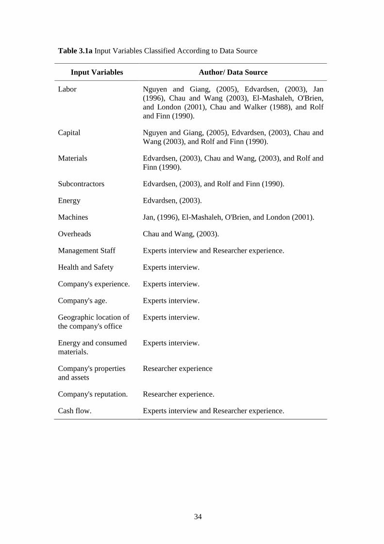
34
Table 3.1a Input Variables Classified According to Data Source
Input Variables Author/ Data Source
Labor Nguyen and Giang, (2005), Edvardsen, (2003), Jan (1996), Chau and Wang (2003), El-Mashaleh, O'Brien, and London (2001), Chau and Walker (1988), and Rolf and Finn (1990).
Capital Nguyen and Giang, (2005), Edvardsen, (2003), Chau and Wang (2003), and Rolf and Finn (1990).
Materials Edvardsen, (2003), Chau and Wang, (2003), and Rolf and Finn (1990).
Subcontractors Edvardsen, (2003), and Rolf and Finn (1990).
Energy Edvardsen, (2003).
Machines Jan, (1996), El-Mashaleh, O'Brien, and London (2001).
Overheads Chau and Wang, (2003).
Management Staff Experts interview and Researcher experience.
Health and Safety Experts interview.
Company's experience. Experts interview.
Company's age. Experts interview.
Geographic location of the company's office
Experts interview.
Energy and consumed materials.
Experts interview.
Company's properties and assets
Researcher experience
Company's reputation. Researcher experience.
Cash flow. Experts interview and Researcher experience.
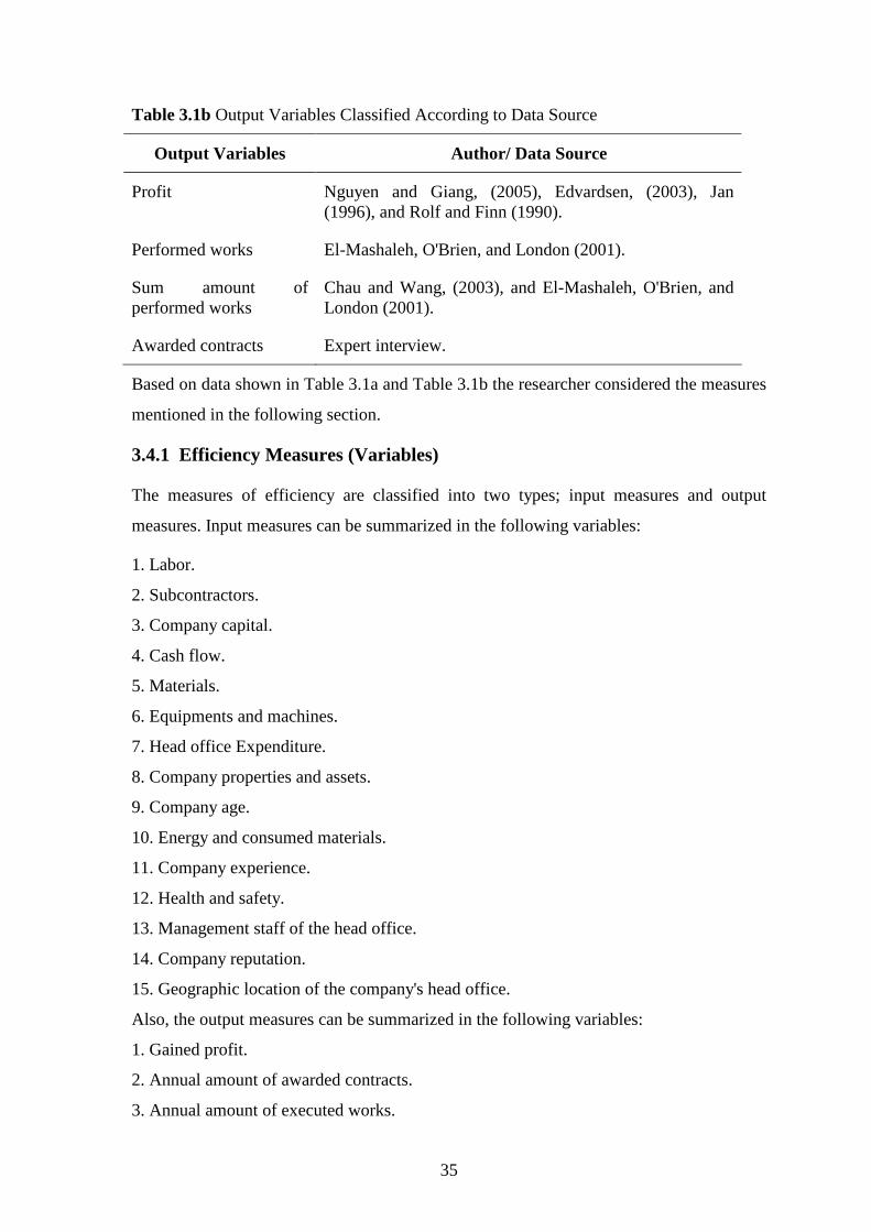
35
Table 3.1b Output Variables Classified According to Data Source
Output Variables Author/ Data Source
Profit Nguyen and Giang, (2005), Edvardsen, (2003), Jan (1996), and Rolf and Finn (1990).
Performed works El-Mashaleh, O'Brien, and London (2001).
Sum amount of performed works
Chau and Wang, (2003), and El-Mashaleh, O'Brien, and London (2001).
Awarded contracts Expert interview.
Based on data shown in Table 3.1a and Table 3.1b the researcher considered the measures
mentioned in the following section.
3.4.1 Efficiency Measures (Variables)
The measures of efficiency are classified into two types; input measures and output
measures. Input measures can be summarized in the following variables:
1. Labor.
2. Subcontractors.
3. Company capital.
4. Cash flow.
5. Materials.
6. Equipments and machines.
7. Head office Expenditure.
8. Company properties and assets.
9. Company age.
10. Energy and consumed materials.
11. Company experience.
12. Health and safety.
13. Management staff of the head office.
14. Company reputation.
15. Geographic location of the company's head office.
Also, the output measures can be summarized in the following variables:
1. Gained profit.
2. Annual amount of awarded contracts.
3. Annual amount of executed works.
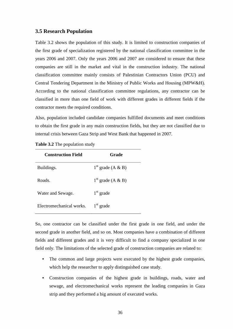
36
3.5 Research Population
Table 3.2 shows the population of this study. It is limited to construction companies of
the first grade of specialization registered by the national classification committee in the
years 2006 and 2007. Only the years 2006 and 2007 are considered to ensure that these
companies are still in the market and vital in the construction industry. The national
classification committee mainly consists of Palestinian Contractors Union (PCU) and
Central Tendering Department in the Ministry of Public Works and Housing (MPW&H).
According to the national classification committee regulations, any contractor can be
classified in more than one field of work with different grades in different fields if the
contractor meets the required conditions.
Also, population included candidate companies fulfilled documents and meet conditions
to obtain the first grade in any main construction fields, but they are not classified due to
internal crisis between Gaza Strip and West Bank that happened in 2007.
Table 3.2 The population study
Construction Field Grade
Buildings. 1st grade (A & B)
Roads. 1st grade (A & B)
Water and Sewage. 1st grade
Electromechanical works. 1st grade
So, one contractor can be classified under the first grade in one field, and under the
second grade in another field, and so on. Most companies have a combination of different
fields and different grades and it is very difficult to find a company specialized in one
field only. The limitations of the selected grade of construction companies are related to:
• The common and large projects were executed by the highest grade companies,
which help the researcher to apply distinguished case study.
• Construction companies of the highest grade in buildings, roads, water and
sewage, and electromechanical works represent the leading companies in Gaza
strip and they performed a big amount of executed works.
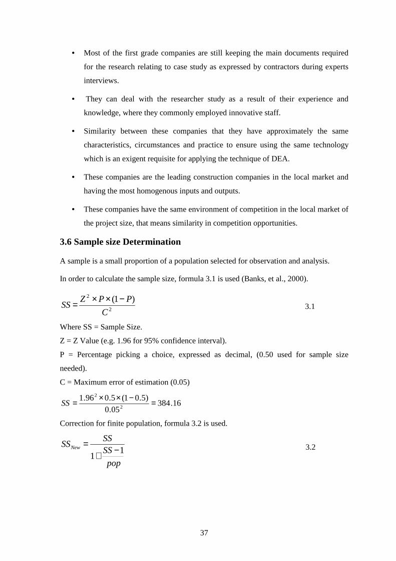
37
• Most of the first grade companies are still keeping the main documents required
for the research relating to case study as expressed by contractors during experts
interviews.
• They can deal with the researcher study as a result of their experience and
knowledge, where they commonly employed innovative staff.
• Similarity between these companies that they have approximately the same
characteristics, circumstances and practice to ensure using the same technology
which is an exigent requisite for applying the technique of DEA.
• These companies are the leading construction companies in the local market and
having the most homogenous inputs and outputs.
• These companies have the same environment of competition in the local market of
the project size, that means similarity in competition opportunities.
3.6 Sample size Determination
A sample is a small proportion of a population selected for observation and analysis.
In order to calculate the sample size, formula 3.1 is used (Banks, et al., 2000).
2
2 )1(
C
PPZSS
−××= 3.1
Where SS = Sample Size.
Z = Z Value (e.g. 1.96 for 95% confidence interval).
P = Percentage picking a choice, expressed as decimal, (0.50 used for sample size
needed).
C = Maximum error of estimation (0.05)
16.38405.0
)5.01(5.096.12
2
=−××=SS
Correction for finite population, formula 3.2 is used.
pop
SSSS
SSNew 11
−+= 3.2

38
Where pop is the population = 48 match the proposed grade of contracting companies
according to the national classification committee for the mentioned years.
4377.42
48
116.3841
16.384 ==−+
=NewSS
The targeted contractors sample, which was determined according to equation 3.2 were
43. Because of limited number of construction companies that represent the population,
the researcher intent to consider a comprehensive population of the 48 companies. Forty
eight questionnaires were printed, but only 42 of them are distributed and received by
companies. The 42 questionnaires were returned fully completed, which represent 98% of
the targeted contractors sample and 88 % of the population. (No ways found to contact
any of the remaining part of 6 companies because of the standstill of construction
activities during the study period due to unjust blockade and companies coercive lockup).
3.7 Data collection
As result of literature review, researcher experience and experts opinion investigation, a
structured questionnaire tool is used for data collection.
3.7.1 Questionnaire Design and Contents
Based on the measures of inputs and outputs related to measuring efficiency of
construction companies generated from combining the results of literature review,
meetings and interviews with general contractor, academic experts, consultants and
researcher experience, a structured questionnaire was developed to facilitate the research
study. All information that could help in achieving the study objectives, were collected,
reviewed and formalized to be suitable for the survey study. The questionnaire aims to
estimate the relative weights of each efficiency variables (measures) to select the most
important variables when apply the technique of DEA in the case study. The mentioned
estimation represents the targeted companies' opinion who are involved and acquainted
with the most resources (inputs) and products (outputs) of their field. After many stages
of brain storming, consulting, amending, and reviewing executed by the researcher with
the supervisors, the research questionnaire was finalized and became ready for
distribution. The questionnaire design was composed of three sections and a cover letter
to motivate the respondents to participate. The three sections are drafted to accomplish
the aim of this research, as follows:
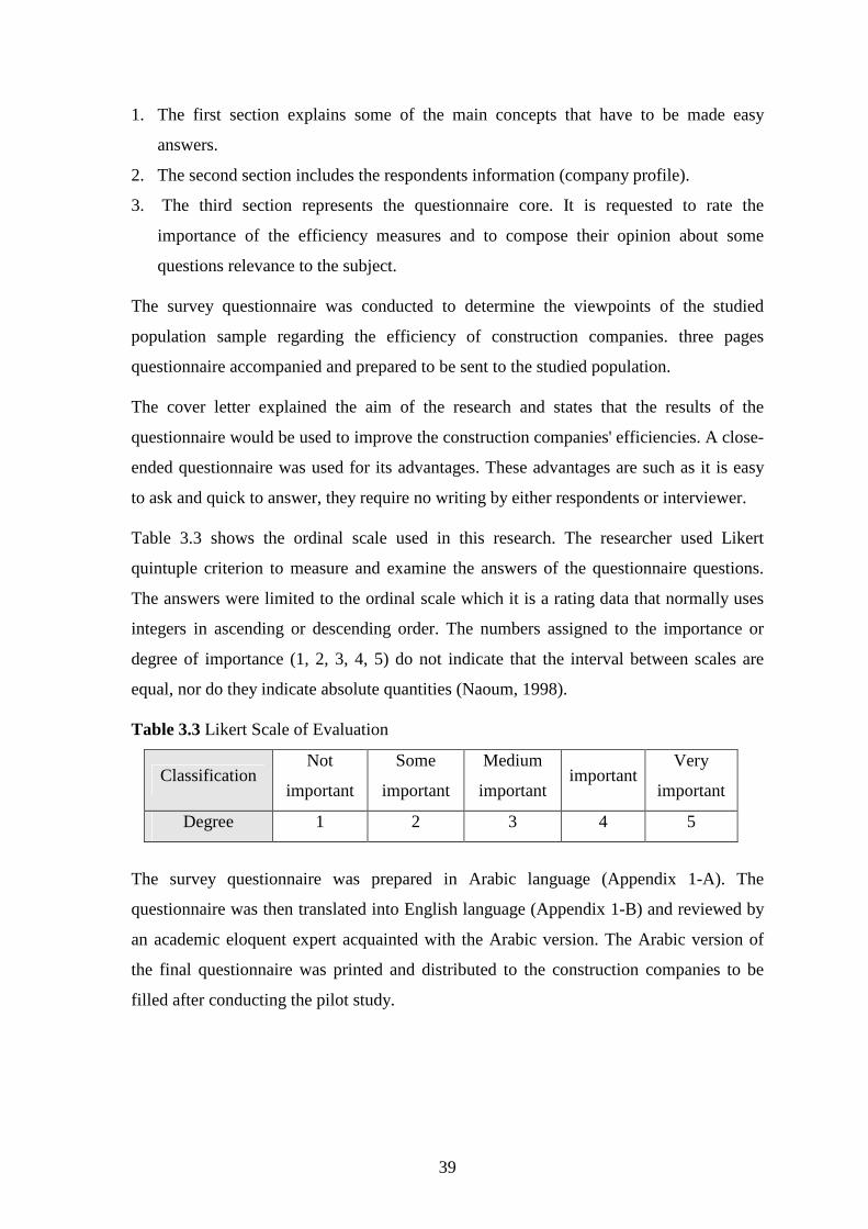
39
1. The first section explains some of the main concepts that have to be made easy
answers.
2. The second section includes the respondents information (company profile).
3. The third section represents the questionnaire core. It is requested to rate the
importance of the efficiency measures and to compose their opinion about some
questions relevance to the subject.
The survey questionnaire was conducted to determine the viewpoints of the studied
population sample regarding the efficiency of construction companies. three pages
questionnaire accompanied and prepared to be sent to the studied population.
The cover letter explained the aim of the research and states that the results of the
questionnaire would be used to improve the construction companies' efficiencies. A close-
ended questionnaire was used for its advantages. These advantages are such as it is easy
to ask and quick to answer, they require no writing by either respondents or interviewer.
Table 3.3 shows the ordinal scale used in this research. The researcher used Likert
quintuple criterion to measure and examine the answers of the questionnaire questions.
The answers were limited to the ordinal scale which it is a rating data that normally uses
integers in ascending or descending order. The numbers assigned to the importance or
degree of importance (1, 2, 3, 4, 5) do not indicate that the interval between scales are
equal, nor do they indicate absolute quantities (Naoum, 1998).
Table 3.3 Likert Scale of Evaluation
Classification Not
important
Some
important
Medium
important important
Very
important
Degree 1 2 3 4 5
The survey questionnaire was prepared in Arabic language (Appendix 1-A). The
questionnaire was then translated into English language (Appendix 1-B) and reviewed by
an academic eloquent expert acquainted with the Arabic version. The Arabic version of
the final questionnaire was printed and distributed to the construction companies to be
filled after conducting the pilot study.
40
3.7.2 Pilot Study
A pilot study was conducted before starting collecting data to test the meaning of the
questions and making sure that the questions are clear and understandable without
duplications in the meanings. It was conducted by distributing the prepared questionnaire
to two panels of experts - having experience in the field of the research - to collect their
remarks on the questionnaire and testing the questionnaire validity. Generally speaking, it
appeared that the two panels had no difficulty in understanding the items to complete the
questionnaire since the questionnaire was studied thoroughly as mentioned before. After
the preliminary testing, a pilot study was conducted to evaluate the questionnaire by
distributing the questionnaire to a sample of 15 companies.
3.7.3 Instrument Validity of the Questionnaire by Arbitrators
The pilot study was conducted by distributing the prepared questionnaire to two panels of
experts having experience in the field of the research to have their remarks on the
questionnaire. The first panel, which consisted of ten experts (two concerned academic
lecturers, one owner, three project managers, one consultants, and four expert
contractors), were asked to verify the validity of the questionnaire topics and its relevance
to the research objective. The second panel, which consists of two experts in statistics,
was asked to identify that the instrument used was valid statistically and that the
questionnaire was designed well enough to provide relations and tests among variables.
Expert comments and suggestions were collected and evaluated carefully. All the
suggested comments and modifications were discussed with the supervisors before taking
them into consideration. At the end of this process, some minor changes, modifications
and additions were introduced to the questions and the final questionnaire was
constructed.
3.7.4 Instrument Validity by Pilot Study
After the preliminary testing, a pilot study was conducted to evaluate the questionnaire.
The researcher distributed the questionnaire to a sample of 15 persons. Generally
speaking, it appeared that the respondents had no difficulty in understanding the items or
the instructions to complete the questionnaire.

41
3.7.5 Instrument Reliability
The reliability coefficient of the scale was established by Cronbach's Alpha using
Statistical Package for the Social Science (SPSS). The reliability coefficient resulted by
Cronbach's Alpha for 15 samples. The reliability coefficient found for input variables is
0.795 and for output variables is 0.922. This range is considered high; the result ensures
the reliability of the questionnaire. The reliability coefficient resulted by Guttman Split-
Half for input variables is 0.822 and for output variables is 0.843 which mean highly
significant.
3.8 Case Study
After analyzing the field survey data, the variables of efficiency and the model are
derived as illustrated in the next chapter. Since the purpose of this study is to measure the
efficiency of construction companies in Gaza Strip, data about the case study were
collected to attain the remaining objectives research. The case study method was applied
to companies which demonstrated a desire to participate in the case study through a
positive reply on question of the questionnaire and the other companies abstained when
they realize that the required data are burdensome.
3.8.1 Case Study Forms
Data of case study is collected through special forms prepared by the cooperation
between a group of 4 general contractors and the researcher to avoid any embarrassing
data. Also, the forms were prepared in Arabic language (Appendix 2-A). The forms were
translated into English language (Appendix 2-B) and reviewed by an academic eloquent
expert acquainted with the Arabic version. The forms aimed to obtain the variables
amount of input and output of construction companies to measure their efficiency. To
achieve the study objectives the illustrated forms in (Appendix 2) are used to collect the
required data.
1. Form (1) and Form (2) Summary of the Company Case Study: it deals with both
input and output variables of the company over the study period of (2002- 2006). It
consists of two parts; the first one (Form 1) summarizes the input variables for each year
of the case study and the annual rate round the years of the study, and the other part
(Form 2) summarizes the components of output variable for each year of the case study
and the annual rate round the years of the study.

42
The inputs of the case study due to the field survey analysis were materials (M), labor
cost (L), cash flow (CF), subcontractors (SUB), equipment and machines (EM), and
management staff of the head office of the company (MS). The output of the case study
was the amount of executed works in the fields of buildings, roads, water and sewage,
electromechanical, and sundries (EW). Both input and output variables of each company
are posted to the summary of the companies case study sub Excel sheet mentioned in
clause 9 hereafter.
2. Form (3) Cost of Used Materials: used materials in this form are classified into the
five years of the study.
3. Form (4) Labors Expenditures: labor expenditures in this form are classified into six
categories of fees for each year of the study; I) project managers, II) engineers, III)
surveyors, foremen, technicians, IV) permanently labors, V) temporary labors, and VI)
additional fees.
4. Form (5) Possessed Cash Flow: in this form the contractor is asked to record
possessed cash flow for each year of the study.
5. Form (6) Amount of Executed Works by Subcontractors: this form is aimed to
count payables payments which they are reflect the amount of executed works by
subcontractors. Payables payments are summed for each year individually and posted to
the input summary of form (1).
6. Form (7) Value of possessed equipments and machines: this form is prepared to
allow contractors to exhibit and estimate the value of possessed equipments and machines
for each year individually.
7. Form (8) Number of Head Office Staff: it is the unique form that reflects a number,
where all other inputs and output are currency except the head office staff is in head
count. It includes all employees, managers, engineers, accountants, secretaries and
servants.
Inputs Forms (3-8) are summed separately and posted to the inputs summary of the form
(1). All mentioned forms (1-8) are belong to the study period, which is limited between
1/1/2002 to 31/12/2006.
8. Form (9) Payable Interim and Final Payments: this Form is aimed to count payables
interim and final payments which they reflect the amount of executed works (output).

43
Payables payments are summed for each year individually and posted to the output
summary in form (2).
To facilitate data gathering, and to motivate respondents to respond, the researcher asked
the companies that have databases and balance sheets about the study period (2002- 2006)
to record only form (1) and form (2).
The nine forms mentioned above were distributed to the participant companies to fill the
required data of the case study.
9. Summary of the Companies Case Study: data were collected by form 1 and form 2
are gathered in the summary of the companies case study. It is the master form, it deals
with both input and output variables of construction companies that participate in the case
study. It consists of six Excel sub sheets. The first sub sheet concerning the first year of
the study (2002), the second concerning the second year of the study (2003), the third part
concerning the third year of the study (2004), the fourth part concerning the fourth year of
the study (2005), the fifth part concerning the fifth year of the study (2006) and last one
concerning the annual rate round the years of the study from (2002) to (2006). These
forms are prepared as Excel sub sheets and shown in the chapter 4, Tables 4.3a, 4.3b,
4.3c, 4.3d, and 4.3e over the years; 2002, 2003, 2004, 2005, and 2006 respectively. Also,
Table 4.4 is an Excel sub sheet shows the averages of input variables over the period
study (for example, one of these Excel sub sheets is shown in this chapter in Table (3.4).
3.8.2 Form Validity
After completion of the tables' forms, the researcher distributed seven of them to
construction companies to investigate its validity. The researcher modified the forms as
advised by the panel, then they attached to a covering letter and distributed to the
companies in Arabic version.

44
Table 3.4 Summary of the Averages of collected variables (2002-2006)
Input Variables
No. Construction
Company M $ L $ CF $ SUB $ EM $ MS No.
Output
Variable
(Amount of
EW $)
1 C1 328514.4 305678.2 124453.8 0 33964.2 10 679285.6
2 C2 636166 134244 60000 396312 32800 5 1279826
3 C3 838000 52400 45000 57600 29600 10.6 1116053.2
4 C4 732607.6 368220.6 163193.8 54923.6 114000 10.8 1318498
5 C5 1134400 343280 0 203800 0 4.8 1870000
6 C6 355000 137000 112000 0 22000 5.2 530000
7 C7 1235200 324000 318000 487000 310000 10 2803400
8 C8 1100000 66000 220000 152000 100000 12 1523000
9 C9 1264000 309760 95787.8 364200 75800 11.2 2239183
10 C10 215974 56470 46000 66310 15000 5 418000
11 C11 323800 115680 76000 211200 42000 5 704000
12 C12 3345600 836400 1618000 1115200 126000 5 5576000
13 C13 2760000 430000 224000 1080000 1673000 23.2 5828800
14 C14 664160.4 110044.4 47200 0 42000 7.2 898577.6
15 C15 2221000 102000 500000 2530000 1580000 13.6 4880000
16 C16 686000 93600 91400 45000 32000 6 916200
17 C17 930500 93050 500000 101500 780000 8 1347500
18 C18 562200 159200 560000 0 125000 5 951156.6
19 C19 1020500 103120 23560 718000 45000 18.4 2063800
20 C20 1977600 139346 128000 2222600 246000 18 4429200
21 C21 440600 111500 91000 197100 140000 5.6 819000
22 C22 808000 171200 37000 733000 134000 7 1807920
Total 23579822.4 4562193.2 5080595.4 10735745.6 5698164.2 206.6 43999400
Average 1071810.11 207372.42 230936.15 487988.44 259007.46 9.391 1999972.7
3.8.3 Participant Companies
This stage mainly depends on identifying a certain number of construction companies
have willingness to participate in the study and providing the required data. The invited
construction companies to participate in the research case study are shown in Table 3.5
The number of companies relative to the number of input and output measures must be

45
large enough to ensure that meaningful efficiency values are obtained. A rule of thumb is
given by Banker et al. (1984) and suggested by Moreno and Tadepalli (2002) as:
3nmk ≤+ Banker et al. (1984) and Moreno and Tadepalli (2002).
nmk ≤× Bowlin (1998).
where k is the number of inputs, m is the number of outputs, and n is the number of
companies (DMUs). Moreover, this rule of thumb is not universally accepted. In this
study, the number of input variables is 6, and only one variable of output. To satisfy the
two above equations, the required number of participant companies is greater than 21, and
6 respectively. Therefore, 22 construction companies participated in the study are
satisfied the above two equations.
3.8.4 Distribution of Case Study Forms
To collect the required data of the case study, the nine Arabic version forms of the case
study was distributed to all invited construction companies mentioned in Table 3.5
through personal interview. The researcher briefly illustrated the objective of the needed
data and explained the suitable way to fill the forms in a sound manner. The interviewees
asked to fill the required data during few days depending on how the time they needed.
The needed time is recorded on researcher's calendar. After the completion of the
recorded needed time, the researcher pursued the respondents through telephone and
mobile to regain the completed forms of case study. Uncompleted forms were given
additional time over and over to obtain more forms as much as possible.
All the forms were reviewed by the researcher to find out incorrect data. Incorrect data
were manipulated after contacting the respondents and some respondents who commit
serious mistakes were asked to correct them and fill new forms. All collected data after
reviewing, manipulating and modified were transcribed in mentioned excel sheets
illustrated in Tables 4.3a, 4.3b, 4.3c, 4.3d, 4.3e, 4.3a and 4.4b.
3.8.5 Case Study Limitations
The limitation of the study period is related to; i) ensure that these companies are still
vital in construction industry; ii) the outbreak of AL-Aqsa Intifada in 2000 succeeded
with a depression period until the last of 2001, then return to relatively revival that enable
the researcher to avoid the depression period; and iii) to ensure that data is still available
and kept by companies for the last years.

46
Table 3.5 Invited Construction Companies
No. Company's Name Location
1 Al-Farra Bro's Khan-Yunis 2 Arrabeta Khan-Yunis 3 Salamat Al-Emar Khan-Yunis 4 Zi-Qar Khan-Yunis 5 Amer Bro's Khan-Yunis 6 Majedco Khan-Yunis 7 Eivel Rafah 8 Ata Sons Rafah 9 Arrewaq Rafah 10 Annael Rafah 11 Salah-Eddin Rafah 12 Abu Shamala Rafah 13 Hatawi Rafah 14 Hjazi Gaza 15 Massoud & Ali Gaza 16 Darweesh Abu Maileq Gaza 17 Ashehabeya Gaza 18 Mushtaha & Hasonna Gaza 19 Palestinian Development Company (PDC) Gaza 20 Abu Ziada Gaza 21 Saqa & Khudhari Gaza 22 Khudhari for Engineering & Contracting Gaza 23 Golden Sand Gaza 24 Abdel-Hakeem Ismael Gaza 25 Abnaa Hashim El-Khozindar Gaza 26 International Bonian Group Gaza 27 Osama K'heel Gaza 28 Abu Dalal Gaza 29 Abu Kmail Sons. Gaza 30 Abu Shamala & Abu Dan Gaza
3.9 Method of Data Analysis
To achieve the research objectives, data analysis focused on identifying issues that may
characterize measures of efficiency. To analyze collected data by questionnaire and forms
of case study, the researcher used two softwares.
The first is the Statistical Package for the Social Science (SPSS) program that used for
manipulating and analyzing the collected data by the questionnaire. The factor analysis
was conducted for both input and output variables. Where the analysis of suggested
variables produce strong variables and excluded the lepto-variables. Analysis of
questionnaire is shown (Appendix 1-C).
47
The second software is the Efficiency Measurement System software package (EMS
version 1.3) that used to measure the relative overall technical efficiency of construction
companies working in Gaza Strip using the technique of DEA under the CCR and BCC
models. Input oriented model was used because the output of the study is out of the
company control. The output is controlled by the employer (owner) and contractors
competition in awarding contracts. Also, the same software is used to find out the
necessary improvements for inefficient companies in order to become efficient. EMS is
free, flexible and can deal with huge number of DMUs. There are many options to use in
model structure such as returns to scale, and model orientation.
EMS, characterized by an advantage of super efficiency scores, that is like the standard
score but the DMU under evaluation is excluded from the constraints.

48
Chapter 4
Results and Analysis
This chapter describes the results obtained from the analysis of field survey and case
study. It is mainly divided into five sections; the first one handles the field survey
statistical results and the approaches used to identify the important measures of
efficiency. The second section tackles selected variables. The third section describes the
model building. Where the fourth section describes case study collected data. Finally, the
fifth section deals with case study results, EMS estimated results, potential improvements
of inefficient DMUs and the findings of the case study objectives.
4.1 Field Survey Statistical Results
4.1.1 Respondents Characteristics
Figure 4.1 shows the characteristics of respondents that participate in the field survey as
follows:
76% of the research data is obtained from the top management companies' members who
occupy a managerial position in the construction companies (chairman, executive
manager or assistant manager), and 24% of data is obtained from project managers of
construction companies. The top level positions of the respondents increases the
confidence and accuracy of the results and also expresses the respondent's high concern to
deal seriously with the case study after.
4.1.2 Determining the Vital Measures of Efficiency
The weighted average and factor analysis approaches were conducted to identify model
variables. In this study, these approaches were adopted and applied on ranking data of the
variables of both inputs and outputs to measure the efficiency as presented in the
questionnaire. The results are discussed in subsequent sections and the appropriate model
that takes into account the most important variables is used to measure the efficiency of
construction companies in Gaza Strip.

49
Project Manager Opinion; 24%
Top Managemant Opinion; 76%
Figure 4.1 Characteristic of Respondents
Approach 1: The Weighted Average Approach
In order to be able to select the appropriate method of analysis, the level of measurement
must be understood. For each type of measurement, there is an appropriate method that
can be applied and not others. In this research, interval scales were used. The scale was
divided into 5 points ranging from 1 (not important) to 5 (very important). Frequency
distribution and the percentage of different items are presented in appendix (1-C).
The respondents were asked to rank the input and output variables according to their
importance by scores from 1 to 5. The most important variables will be selected and used
in building the model that measures the relative efficiency of construction companies in
Gaza Strip.
To determine the relative ranking of the variables, these scores were then transformed to
importance indices based on the formula 4.1 (Daniel, 1991).
N
nnnnn
N
WAverage 12345 2345 ++++== ∑ 4.1
Where;
∑W , weighted sum of the variable.
N, the total number of respondents.
1n , the number of respondents who answered "not important".
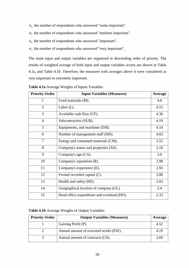
50
2n the number of respondents who answered "some important".
3n the number of respondents who answered "medium important".
4n the number of respondents who answered "important".
5n the number of respondents who answered "very important".
The main input and output variables are organized in descending order of priority. The
results of weighted average of both input and output variables scores are shown in Table
4.1a, and Table 4.1b. Therefore, the measures with averages above 4 were considered as
very important to extremely important.
Table 4.1a Average Weights of Inputs Variables
Average Input Variables (Measures) Priority Order
4.6 Used materials (M). 1
4.55 Labor (L). 2
4.36 Available cash flow (CF). 3
4.19 Subcontractors (SUB). 4
4.14 Equipments, and machines (EM). 5
4.02 Number of management staff (MS). 6
3.52 Energy and consumed materials (CM). 7
3.10 Company's assets and properties (AS). 8
3.0 Company's age (CA). 9
2.98 Company's reputation (R). 10
2.93 Company's experience (E). 11
2.88 Formal recorded capital (C). 12
2.83 Health and safety (HS). 13
2.4 Geographical location of company (GL). 14
2.33 Head office expenditure and overhead (HO). 15
Table 4.1b Average Weights of Output Variables
Average Output Variables (Measures) Priority Order
4.52 Gaining Profit (P). 1
4.19 Annual amount of executed works (EW). 2
2.69 Annual amount of contracts (CS). 3

51
Approach 2: Factor Analysis for Main Measures of Efficiency
This technique was applied in this study to identify a relatively small number of variables
that can be used to represent relationships among other variables. In the following section
variables extraction method is used to determine the number of variables to represent the
efficiency measures.
Variables Extraction
To determine how many variables will be needed to represent the data, the 15 input
variables and the three output variables were assumed to be independent variables. The
percentage of total variance of each variable is examined. The total variance is the sum of
the variances of each variable. Since both the 15 variables of input and 3 variables of
output are standardized to have a variance of 1, so the total variances are 15 and 3
respectively.
Table 4.2a and Table 4.2b show the statistical analysis for input and output variables. The
total variance explained by each variable is listed in the column labeled "Eigen value".
The next column contains the percentage of the total variance attributable to each
variable. For example, variable 2 has a variance of 2.37 which is 15.80 percent of the total
variance of 15. The last column, the cumulative percentage, indicates the percentage of
variance attributable to that variable and those that precede it in the Table.
The Common procedure has been proposed for determining the number of variables to
use in a model is that only the variables that account for variance greater than 1 (Eigen
value greater than 1 should be included) (Chan and Tam, 2000).
Table 4.2a shows that almost 75.00 percent of the total variance of the input variables is
attributed to the first 6 variables where each variable has an Eigen value greater than 1.
The remaining 9 variables together account for only 25 percent of the variance. Also,
Table 4.2b shows that almost 57 percent of the total variance of the output variables is
attributed to only one variable where each variable has an Eigen value greater than 1. the
remaining 2 variables together account for only 43 percent of the variance. Thus a model
with 6 variables of input and one variable of output can be considered adequate to
represent the data.

52
Table 4.2a Statistical Analysis of the Input Variables for Factor Analysis
Communality New
Variable
Total Variance
(Eigen Value)
Percentage
Variance
Cumulative
Percentage
1.00 1 3.20 21.33 21.33
1.00 2 2.37 15.80 37.13
1.00 3 1.95 13.00 50.13
1.00 4 1.42 9.47 59.60
1.00 5 1.22 8.13 67.73
1.00 6 1.09 7.27 75.00
1.00 7 0.89 5.93 80.930
1.00 8 0.63 4.20 85.13
1.00 9 0.58 3.87 89.00
1.00 10 0.50 3.33 92.33
1.00 11 0.37 2.47 94.80
1.00 12 0.28 1.87 96.67
1.00 13 0.20 1.33 98.00
1.00 14 0.16 1.07 99.07
1.00 15 0.14 0.93 100.00
Table 4.2b Initial Statistical Analysis of the Output Variables for Factor Analysis
Communality New
Variable
Total Variance
(Eigen Value)
Percentage
Variance
Cumulative
Percentage
1 1 1.709 57 57
1 2 0.993 33.10 90.10
1 3 0.298 9.90 100.000
Also, Fig. 4.2a and Fig. 4.2b show scree plots of the total variance associated with each
variable of input and output variables.

53
Figure 4.2a Input Variables Scree plot
Figure 4.2b Output Variables Scree Plot

54
4.2 Selected Variables
The first and arguably the most important step in carrying out the measurement of
companies efficiency, is the identification of the input and output variables
(Thanassoulis, 2003). However, it is worth to observe that there is no consensus on the
issue which are the most appropriate variables to be applied in the analysis. As Paradi and
Schaffnit (2004) noticed – "choice of inputs and outputs for DEA models is the subject of
a never ending debate".
Based on the results mentioned earlier of this chapter, the researcher suggests to consider
6 input variables and only one output variables. The six input variables have the highest
average weights of the input variables are shown in Table 4.1a. The suggested unique
variable of output is the amount of executed works. Its average weight ranked second as it
is shown in Table 4.1b.
Yet, the researcher was obliged to disregard the most important variable of output
variables (profit) and consider the second important one (amount of executed works). The
justifications of the decision are related to:
1. During the contractor's opinion investigation stage mentioned in chapter 3,
interviewees indicated that many construction companies (contractors) feel
embarrassed when they are asked about profits and delay damages. They also,
declare that they will not give information about profits . Some of them added that
they will give a false number if they are asked about.
2. Practically, the amount of executed works has a very tied relationship with gained
profits, where profits in most cases are taken as a percentage of the contract
amount. Profit may be increase or drop due to the existing state of the company.
The existing state has a high connection to the amount of bids, amount of projects
under execution, financial capacity of the company, currency fluctuation and other
special or political conditions. Also, the statistical analysis shows a positive
significance between profits and executed works, where the correlation factor
between them was found to be 0.666 as shown in (Appendix 1-C).
So, these variables of both inputs and output are considered as the base of the model
building.

55
4.2.1 Description of Variables
The relationship between the number of departments (DMUs) and the number of
performance measures is important. The number of departments relative to the number of
input and output measures must be large enough to ensure that meaningful efficiency
values are obtained. The number of both input and output variables depends mainly on
the number of companies (DMUs). The least required number to apply DEA was
identified earlier in chapter 3 to be 21 DMUs.
I. Input Variables
1- Used Materials (M)
There is an impossibility to find a common homogenous unit that gathers between all
types of materials, where some materials purchased by cubic meters, meter length,
weight, or by pieces and so on. Therefore, the researcher considered materials cost as a
common attribute.
2- Labor (L)
During contractors opinion investigation mentioned in chapter 3, it was investigated a
lack of document about labor account or working days or hours. Only the available data
about labor was the cost. So, the researcher was forced to consider labor cost as a
rationale measure for all companies with the regard to the fact that all companies has the
same rate of wages.
3- Cash Flow (CF)
In view of the fact that, the formal recorded capital of the companies does not reflect the
financial capacity of construction company as it was investigated. The capital is recorded
based on the contractors' satisfaction. Field study investigation reflected the significance
of the cash flow to be considered. Cash flow is defined as the company balance and
possessed money in the beginning of the year.
4- Subcontractors (SUB)
Numerous companies depend on subcontractors in achieving their activities partially or
wholly. In most cases, some of construction activities need specialist contractors
(subcontractors) who has superior experience in their fields and possessed equipment,
machines, and technicians. Other contractors who do not have equipment and machines
were executed the works activities by subcontractors.

56
5- Equipment and Machines (EM)
The pilot study showed lack of document about equipment and machines hours, sum of
depreciation value of the owned equipment and machines and average maintenance
expenses. To overcome the lack of depreciation of equipment and machines value, the
researcher considered the equipments and machines value at the beginning of the year to
be as an indicator of their contribution to produce output.
6- Management Staff (MS):
It can be represented by the number of management staff in the head office that consists
of top management, assistants, engineers, accountants, secretary, servants, and so on.
Management staff is the responsible party of purchases, contracting, bidding, supreme
supervision, supplying materials and technical support activities for different sites of the
executed works. Number of management staff is considered because it is easy to obtain
rather than cost because the cost encompasses with ambiguities. Cost management staff
ambiguities return to companies policy, where some companies assign salary for every
one of the management staff including sharers where other exclude the sharers.
II Output Variables:
1. Profit
Profit has the first weight of the output variables, it was excluded due to justification
mentioned earlier. Worth mentioning, the correlation factor between profits and executed
works equal 0.666 which means that there is a positive relation between profits and
executed works.
2. Annual Amount of Executed Works (EW)
Executed works have the second weight (average) of output variables, where the first one
is the profit. The first variable is excluded because the contractors expressed in the
contractor's opinion investigation mentioned earlier in chapter 3 that they are not willing
to declare their profits and this variable is considered as a very private and top secret. The
researcher substitutes the profit variable by the annual amount of executed works. The
annual amount of executed works have a very tied relationship with profits, where profits
in most cases are taken as percent of the contract amount.
Noteworthy, the output variables are expressed by the physical quantity of products.
Commonly, physical products of construction companies are numerous, where contracts

57
are sometimes square meter, cubic meter, meter length, unit price and lump sum.
Therefore, the annual amount of executed works is the most appropriate common
attribute to express about output and can be considered as an indicator about the gained
profits.
Now, after the researcher investigated the most variables that have to be considered in the
research, the model can be built.
4.3 Model Building
The developed model philosophy is suggested to be based upon the following:
• Efficiency measurement is the trigger for performance improvement.
• The concept of efficiency and performance changes due to time, environment,
technology advancement and improvements.
• Efficiency means perform everything efficiently from start to perfect completion.
The study mainly aims to measure the technical efficiency of construction companies
which reflects the maximal outputs from a given set of inputs or the minimal inputs to
produce a given set of outputs.
Hence, with the inputs and outputs identified in the previous section, DEA model can be
formulated based on virtual inputs and virtual outputs as follows:
Virtual Inputs
GLRMSHSECMCAASHOEMMCFCSUBLInput ++++++++++++++=
EWCSPOutputs ++=
inputs of sum Weightedoutputs of sum Weighted=Efficiency
GLvRvMSvHSvEvCMvCAvASvHOvEMvMvCFvCvSUBvLv
EWuCSuPuE
151413121110987654321
321
++++++++++++++++
=
The above general formula can be converted into an improved (compact) model
considering the earlier mentioned important variables as below:
MSvEMvSUBvCFvLvMv
uEWE
654321 +++++= 4.1
Where:

58
E: Relative Efficiency of Construction Company.
EW: Annual Amount of Executed Works (Output).
M: Material Cost.
L: Labor Cost.
CF: Available Cash Flow.
SUB: Subcontractors Cost.
EM: Value of Owned Equipments and Machines.
MS: Total Number of Management Staff.
u : Given Weight to output.
654321 ,,,,, vvvvvv : Given Weights to Inputs.
Transformation of the above fractional form into a linear programming as done by
Charnes et al. (1978) for the current study which consists of 22 construction companies
producing one output using six different inputs.
0
6
1i
ii xvMin ∑
=
=θ
Subject to
10 =yu ,
06
1
≥−∑=
jjiji
ij yuxv , 22,....,2,1=j
0, ≥ijj vu
Where, θ is the optimal objective value.
Since the amount of executed works in construction sector is out of the company control
because the amount of contracts often yields to the client's visibility, tendering process
and invitation of offers which means that the amount of executed works is determined by
clients.
As such, our model takes an input-oriented rather than an output-oriented approach. Both
CCR and BCC input oriented model are applied to have high flexibility in choosing

59
between them. Using these models is very important in order to check whether all DMUs
work at optimal scale or not. If the DMUs work at optimal scale then CCR model must be
used otherwise BCC model must be used.
4.4 Case Study Data
As mentioned in the research methodology, data was collected in the following five
Tables; 4.3a, 4.3b, 4.3c, 4.3d, and 4.3e over the years of 2002, 2003, 2004, 2005, and
2006 respectively. Table 4.4 represents the averages of collected variables of input and
output of the mentioned study period (2002-2006). These Tables mainly contain the
selected input and output variables. The selected input variables are material (M), labor
(L), cash flow (CF), subcontractors (SUB), equipments and machines (EM), and
management staff where the unique selected output variable is executed works (EW).

60
Table 4.3a Values of Input and Output Variables in Year (2002)
Input Variables No. DMUs
M $ L $ CF $ SUB $ EM $ MS No.
Amount of EW $
1 C1 0 0 0 0 0 10 0
2 C2 213650 54750 50000 128360 22000 5 429940
3 C3 750000 50000 45000 50000 30000 10 1002087
4 C4 419930 206850 150764 17400 100000 6 742799
5 C5 492000 16400 0 41000 0 2 820000
6 C6 290000 110000 50000 0 10000 5 450000
7 C7 863000 222000 320000 465000 315000 10 2138000
8 C8 1600000 80000 100000 250000 100000 10 2275000
9 C9 1435000 362800 39720 400000 55000 10 2570000
10 C10 182300 60000 35000 57000 15000 4 360000
11 C11 48600 20400 60000 36000 30000 3 120000
12 C12 2628000 657000 1500000 876000 120000 4 4380000
13 C13 1700000 250000 100000 400000 1300000 20 2860000
14 C14 811730 135942 35000 0 40000 7 1033324
15 C15 1952000 102000 400000 2000000 1300000 12 4500000
16 C16 550000 90000 55000 110000 25000 6 822000
17 C17 * * * * * * *
18 C18 90000 26000 500000 0 68000 5 120000
19 C19 1203500 130000 25000 680000 50000 16 2075000
20 C20 2790000 188900 140000 1966000 270000 18 5010000
21 C21 518000 155000 110000 186000 160000 5 968000
22 C22 1886000 218000 23000 789000 110000 7 2993000
* Data about this company was unavailable.

61
Table 4.3b Values of Input and Output Variables in Year (2003)
Input Variables No. DMUs
M $ L $ CF $ SUB $ EM $ MS No.
Amount of EW $
1 C1 526157 479425 213078 0 53270 10 1065392
2 C2 371300 63460 50000 298400 30000 5 819770
3 C3 670000 47000 55000 53000 28000 10 889881
4 C4 373978 190456 140771 44118 100000 6 687017
5 C5 840000 260000 0 103000 0 3 1290000
6 C6 175000 65000 70000 0 10000 5 250000
7 C7 1520000 367000 320000 428000 315000 10 3037000
8 C8 0 0 100000 0 100000 10 0
9 C9 910000 234000 73219 250000 55000 10 1785000
10 C10 214800 65800 50000 67000 15000 5 430000
11 C11 692000 255000 100000 450000 50000 6 1500000
12 C12 2280000 570000 1520000 760000 120000 5 3800000
13 C13 3000000 550000 170000 800000 1300000 22 11384000
14 C14 739743 166584 104000 0 40000 7 1022867
15 C15 2398000 98000 400000 2500000 1300000 12 5400000
16 C16 410000 65000 75000 60000 35000 6 604000
17 C17 * * * * * * *
18 C18 735000 208000 500000 0 68000 5 1177783
19 C19 1364000 115600 15000 550000 25000 16 2565000
20 C20 1860000 162000 160000 2375000 270000 18 4446000
21 C21 426000 123000 125000 214000 140000 6 830000
22 C22 541000 138000 27000 860000 110000 7 1638300
* Data about this company was unavailable.
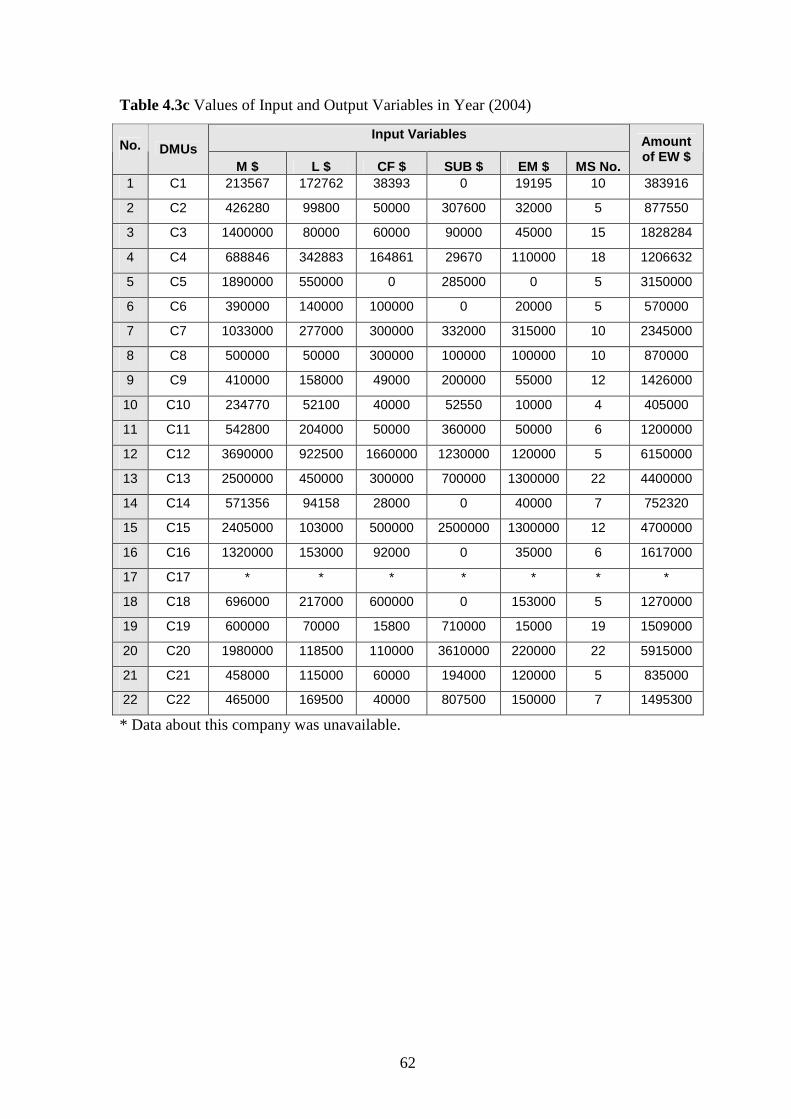
62
Table 4.3c Values of Input and Output Variables in Year (2004)
Input Variables No. DMUs
M $ L $ CF $ SUB $ EM $ MS No.
Amount of EW $
1 C1 213567 172762 38393 0 19195 10 383916
2 C2 426280 99800 50000 307600 32000 5 877550
3 C3 1400000 80000 60000 90000 45000 15 1828284
4 C4 688846 342883 164861 29670 110000 18 1206632
5 C5 1890000 550000 0 285000 0 5 3150000
6 C6 390000 140000 100000 0 20000 5 570000
7 C7 1033000 277000 300000 332000 315000 10 2345000
8 C8 500000 50000 300000 100000 100000 10 870000
9 C9 410000 158000 49000 200000 55000 12 1426000
10 C10 234770 52100 40000 52550 10000 4 405000
11 C11 542800 204000 50000 360000 50000 6 1200000
12 C12 3690000 922500 1660000 1230000 120000 5 6150000
13 C13 2500000 450000 300000 700000 1300000 22 4400000
14 C14 571356 94158 28000 0 40000 7 752320
15 C15 2405000 103000 500000 2500000 1300000 12 4700000
16 C16 1320000 153000 92000 0 35000 6 1617000
17 C17 * * * * * * *
18 C18 696000 217000 600000 0 153000 5 1270000
19 C19 600000 70000 15800 710000 15000 19 1509000
20 C20 1980000 118500 110000 3610000 220000 22 5915000
21 C21 458000 115000 60000 194000 120000 5 835000
22 C22 465000 169500 40000 807500 150000 7 1495300
* Data about this company was unavailable.

63
Table 4.3d Values of Input and Output Variables in Year (2005)
Input Variables No. DMUs
M $ L $ CF $ SUB $ EM $ MS No.
Amount of EW $
1 C1 78504 83817 18626 0 9313 10 186260
2 C2 782100 174260 80000 557900 40000 5 1718720
3 C3 500000 30000 40000 35000 15000 10 698500
4 C4 1879637 943738 162921 113422 130000 18 3345902
5 C5 1100000 400000 0 190000 0 6 1860000
6 C6 320000 130000 140000 0 20000 5 480000
7 C7 1070000 350000 300000 790000 315000 10 3123000
8 C8 1700000 100000 300000 170000 100000 15 1870000
9 C9 1630000 306000 197000 400000 107000 12 2398915
10 C10 243000 47800 50000 82000 20000 6 445000
11 C11 312200 90500 120000 195000 40000 5 650000
12 C12 3270000 817500 1690000 1090000 120000 5 5450000
13 C13 3100000 400000 350000 1500000 2300000 24 4500000
14 C14 661745 51510 17000 0 45000 7 867087
15 C15 2248000 108000 600000 3000000 2000000 16 5500000
16 C16 620000 85000 110000 55000 25000 6 853000
17 C17 136000 107000 500000 61800 750000 8 340000
18 C18 460000 110000 600000 0 168000 5 780000
19 C19 980000 90000 27000 540000 60000 21 1670000
20 C20 1890000 125330 100000 1737000 220000 17 3898000
21 C21 297000 88000 80000 223000 130000 6 660000
22 C22 542000 204500 45000 695000 150000 7 1575000
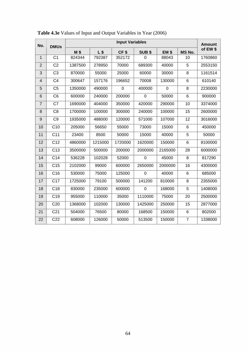
64
Table 4.3e Values of Input and Output Variables in Year (2006)
Input Variables No. DMUs
M $ L $ CF $ SUB $ EM $ MS No.
Amount of EW $
1 C1 824344 792387 352172 0 88043 10 1760860
2 C2 1387500 278950 70000 689300 40000 5 2553150
3 C3 870000 55000 25000 60000 30000 8 1161514
4 C4 300647 157176 196652 70008 130000 6 610140
5 C5 1350000 490000 0 400000 0 8 2230000
6 C6 600000 240000 200000 0 50000 6 900000
7 C7 1690000 404000 350000 420000 290000 10 3374000
8 C8 1700000 100000 300000 240000 100000 15 2600000
9 C9 1935000 488000 120000 571000 107000 12 3016000
10 C10 205000 56650 55000 73000 15000 6 450000
11 C11 23400 8500 50000 15000 40000 5 50000
12 C12 4860000 1215000 1720000 1620000 150000 6 8100000
13 C13 3500000 500000 200000 2000000 2165000 28 6000000
14 C14 536228 102028 52000 0 45000 8 817290
15 C15 2102000 99000 600000 2650000 2000000 16 4300000
16 C16 530000 75000 125000 0 40000 6 685000
17 C17 1725000 79100 500000 141200 810000 8 2355000
18 C18 830000 235000 600000 0 168000 5 1408000
19 C19 955000 110000 35000 1110000 75000 20 2500000
20 C20 1368000 102000 130000 1425000 250000 15 2877000
21 C21 504000 76500 80000 168500 150000 6 802000
22 C22 608000 126000 50000 513500 150000 7 1338000

65
Table 4.4 Summary of the Averages of the Variables Values (2002-2006)
Input Variables No. DMUs
M $ L $ CF $ SUB $ EM $ MS No.
Amount of EW $
1 C1 328514.4 305678.2 124453.8 0 33964.2 10 679285.6
2 C2 636166 134244 60000 396312 32800 5 1279826
3 C3 838000 52400 45000 57600 29600 10.6 1116053.2
4 C4 732607.6 368220.6 163193.8 54923.6 114000 10.8 1318498
5 C5 1134400 343280 0 203800 0 4.8 1870000
6 C6 355000 137000 112000 0 22000 5.2 530000
7 C7 1235200 324000 318000 487000 310000 10 2803400
8 C8 1100000 66000 220000 152000 100000 12 1523000
9 C9 1264000 309760 95787.8 364200 75800 11.2 2239183
10 C10 215974 56470 46000 66310 15000 5 418000
11 C11 323800 115680 76000 211200 42000 5 704000
12 C12 3345600 836400 1618000 1115200 126000 5 5576000
13 C13 2760000 430000 224000 1080000 1673000 23.2 5828800
14 C14 664160.4 110044.4 47200 0 42000 7.2 898577.6
15 C15 2221000 102000 500000 2530000 1580000 13.6 4880000
16 C16 686000 93600 91400 45000 32000 6 916200
17 C17 930500 93050 500000 101500 780000 8 1347500
18 C18 562200 159200 560000 0 125000 5 951156.6
19 C19 1020500 103120 23560 718000 45000 18.4 2063800
20 C20 1977600 139346 128000 2222600 246000 18 4429200
21 C21 440600 111500 91000 197100 140000 5.6 819000
22 C22 808000 171200 37000 733000 134000 7 1807920
Total 23579822 4562193 5080595 10735746 5698164 206. 43999400
Average 1071810 207372 230936 487988 259007 9.39 1999972.7

66
4.5 Case Study Results
4.5.1 Sample Characteristics
Table 4.5 shows a statistical results of the input and output variables. The type and
number of variables are listed in the column labeled “Type”. For example “I1” means the
first input and “O” means the unique output. Significant differences were found between
construction companies in the case study. For instance the input of the materials per year
ranged between $215974 and $3345600 with an average of $1071810. Labors cost per
year ranged between $52400 and $836400 with an average of $207372. Utilized cash
flow per year ranged between $0.0 and $1618000 with an average of $230936.
Subcontractors cost per year ranged between $0.0 and $2530000 with an average of
$487988. Owned equipments and machines value per year ranged between $0.0 and
$1673000 with an average of $259007. Number of management staff per year ranged
between 4.8 and 23.2 persons with an average of 9.4 persons.
Also, Table 4.5 shows at the last row the significant difference of output, where the
amount of executed works ranged between 418000$ and 5828800$ with an average of
$1999973.
Table 4.5 Statistical Results of the Input and Output Variables
Type
(I/O)
Variable Min
Max Average Std. Dev.
I1 Used Materials (M). 215974 $ 3345600 $ 1071810 $ 816866
I2 Labors (L). 52400 $ 836400 $ 207372 $ 180439
I3 Cash Flow (CF). 0 1618000 $ 230936 $ 349997
I4 Subcontractors (SUB). 0 2530000 $ 487988 $ 699076
I5 Equipments & machines (EM). 0 1673000 $ 259007 $ 472716
I6 Management staff (MS). 4.8 P 23.2 P 9.4 P 5.124 P
O Executed Works (EW). 418000 $ 5828800 $ 1999973 $ 1658905 $
Table 4.6 shows the average contribution of each field of executed works associated with
the companies and their percentage during the period (2002- 2006). Also, Fig 4.3 shows
the same result in pie chart shape.

67
Table 4.6 Fields Contribution to Executed Works
Projects
Type Buildings Roads W & S Ele-Mech Sundries Total
Amount $ 19714806.6 13273589 5268164 5443280.8 299559.6 43999400
Percent % 44.8 % 30.1 % 12 % 12.4 % 0.7 % 100 %
Buildings 44.80%
Roads 30.10%
W & S 12%
Ele-Mech 12.40%
Sundries 0.70%
Figure 4.3 Output's Components of executed works
4.5.2 Results and Analysis of DEA
Efficiency Measurement System (EMS) software "version 1.3" is used in this research to
evaluate the relative technical efficiency of construction companies based on both CCR
and BCC input oriented models. It is also used to find out the needed potential
improvements of inefficient companies in order to reach 100% efficiency.
EMS is free, flexible and can deal with huge number of DMUs. There are many options
to use in model structure, return to scale, distance and model orientation. It successfully
solved problems with over 5000 DMUs and about 40 inputs and outputs. It accepts data in
MS Excel or in text format, EMS accepts Excel 97 and older. The inputs and outputs data
should be collected in one work sheet and the user asked not to use formulas in this sheet,
it should be only contain the pure data and nothing else. Some notes about dealing with
EMS are follows:
o The name of the worksheet must be "Data".

68
o The first line contains the input/output names. First inputs, then outputs.
o Inputs names contain the string "{I}".
o Outputs names contain the string "{O}".
o The first column contains the DMUs names.
The output of EMS contains score of each DMU, weights, benchmarks, reference
sets as shown in snapshot in Fig. 4.4.
Fig. 4.4 EMS Outputs of 2006.
The DEA model will measure efficiency scores with CRS technology (or overall
technical efficiency, or CCR) and VRS technology (or technical efficiency, or BCC).
CCR gives a measure of overall efficiency of each DMU, such that technical efficiency
and scale efficiency are aggregated into one value. CCR model assumes that there are
constant returns to scale (i.e. an increase in inputs results in a proportionate increase in
outputs). Also, it assumes that all DMUs work at optimal scale. BCC model measures
pure technical efficiency and assumes that there are variable returns to scale which
includes increasing returns to scale and decreasing returns to scale.
The reference set represents the peer DMUs when compared with other DMUs and
becomes its benchmark. DMUs which have benchmarks are asked to learn how to transfer
their inputs to outputs, in other words, adopt their policies and techniques in the
production process. In the following sections, the CCR and BCC models were used to
calculate the efficiency scores of DMUs.

69
1. CCR Results
Table 4.7 shows the CRS results. The overall technical efficiency of (CRS) scores
average of construction companies over the study period was 94.4%.
Table 4.7 DMUs Overall Technical Efficiency (CCR) Scores over Time
DMUs Established
Year
2002
Score
2003
Score
2004
Score
2005
Score
2006
Score
C1 1995 0.00% 100% 100% 100% 100%
C2 1985 100% 97.4% 83.1% 100% 100%
C3 1991 83.7% 100% 100% 100% 100%
C4 1994 100% 66.7% 98.7% 100% 93.89%
C5 1999 100% 100% 100% 100% 100%
C6 1994 100% 100% 100% 100% 100%
C7 1980 100% 74.9% 100% 100% 100%
C8 1994 81.2% 0.00% 100% 98.6% 100%
C9 1996 100% 98.8% 100% 89.5% 90.4%
C10 1995 100% 96.7% 87.8% 96.4% 100%
C11 1994 99.7% 100% 90.5% 88.% 90%
C12 1987 100% 100% 100% 100% 100%
C13 1988 92.2% 100% 94.7% 81.7% 91.3%
C14 1995 100% 100% 100% 100% 100%
C15 1984 100% 100% 100% 100% 100%
C16 1996 82.3% 81.9% 100% 100% 100%
C17 1994 * * * 92.3% 100%
C18 1996 93.1% 100% 100% 100% 100%
C19 1994 99.1% 100% 100% 100% 100%
C20 1985 99.8% 100% 100% 100% 100%
C21 1994 87.5% 58.0% 80.4% 78.8% 84.1%
C22 1994 100% 100% 100% 100% 99.7%
Average -- 91.4% 89.3% 96.9% 96.6% 97.7%
Efficient DMUs (No.)
-- 11 13 15 15 16
Inefficient DMUs (No.)
-- 10 8 6 7 6
Average Overall Technical Efficiency Score over the Study Period = 94.4%
* Data about this Company was Unavailable.

70
2. BCC Results
Table 4.8 shows the VRS results. The pure technical efficiency of VRS scores average of
construction companies over the study period was 98.9%.
Table 4. 8 DMUs Technical Efficiency (BCC) Scores over Time
DMUs Established
Year
2002
Score
2003
Score
2004
Score
2005
Score
2006
Score
C1 1995 100% 100% 100% 100% 100%
C2 1985 100% 100% 99.2% 100% 100%
C3 1991 100% 100% 100% 100% 100%
C4 1994 100% 87.7% 100% 100% 99.9
C5 1999 100% 100% 100% 100% 100%
C6 1994 100% 100% 100% 100% 100%
C7 1980 100% 75% 100% 100% 100%
C8 1994 100% 100% 100% 100% 100%
C9 1996 100% 99% 100% 100% 100%
C10 1995 100% 100% 100% 100% 100%
C11 1994 100% 100% 99.2% 100% 100%
C12 1987 100% 100% 100% 100% 100%
C13 1988 92.2% 100% 94.7% 100% 100%
C14 1995 100% 100% 100% 100% 100%
C15 1984 100% 100% 100% 100% 100%
C16 1996 83.1% 100% 100% 100% 100%
C17 1994 * * * 100% 100%
C18 1996 100% 100% 100% 100% 100%
C19 1994 100% 100% 100% 100% 100%
C20 1985 100% 100% 100% 100% 100%
C21 1994 89.4% 85.9% 94% 100% 94.5%
C22 1994 100% 100% 100% 100% 100%
Average -- 98.3 97.5% 99% 100% 99.7
Efficient DMUs (No.)
-- 18 17 17 22 20
Inefficient DMUs (No.)
-- 3 4 4 0 2
Average Technical Efficiency Score over the Study Period = 98.9%
* Data about this Company was Unavailable.

71
3. Scale Efficiency Analysis
Table 4.9 DMUs Scale Efficiency Scores over Time
DMUs Established
Year
2002
Score
2003
Score
2004
Score
2005
Score
2006
Score
C1 1995 0.00% 100% 100% 100% 100%
C2 1985 100% 97.4% 83.8% 100% 100%
C3 1991 83.7% 100% 100% 100% 100%
C4 1994 100% 76% 98.7% 100% 94%
C5 1999 100% 100% 100% 100% 100%
C6 1994 100% 100% 100% 100% 100%
C7 1980 100% 100% 100% 100% 100%
C8 1994 81.2% 0.00% 100% 98.6% 100%
C9 1996 100% 100% 100% 89.5% 90.4%
C10 1995 100% 96.7% 87.8% 96.4% 100%
C11 1994 99.7% 100% 91% 88% 90%
C12 1987 100% 100% 100% 100% 100%
C13 1988 100% 100% 94.7% 81.7% 91.3%
C14 1995 100% 100% 100% 100% 100%
C15 1984 100% 100% 100% 100% 100%
C16 1996 99% 81.9% 100% 100% 100%
C17 1994 * * * 92.3% 100%
C18 1996 93.1% 100% 100% 100% 100%
C19 1994 99.1% 100% 100% 100% 100%
C20 1985 99.8% 100% 100% 100% 100%
C21 1994 97.87% 68% 85% 78.8% 89%
C22 1994 100% 100% 100% 100% 99.7%
Average ---- 93% 91.4% 97% 96.6% 97.9%
Average Scale Efficiency Score over the Study Period = 95.2%
* Data about this Company was Unavailable.
As mentioned in chapter 2, overall technical efficiency can be decomposed to technical
efficiency and scale efficiency. The ratio of overall technical efficiency to technical
efficiency is called scale efficiency, which measures the inefficiency caused by
inappropriate scale. In this research , overall technical efficiency refers to CCR scores and
technical efficiency refers to BCC scores where the scale efficiency will be overall
technical efficiency divided by technical efficiency. Table 4.9 shows the scale efficiency
scores of DMUs over the study period. The average scale efficiency was 95.2 percent
which means that the ability to work at optimal scale is 95.2%.

72
4. CCR Versus BCC Results
The results of CCR and BCC models is that the CCR model generates a number of
efficient companies less than BCC model. The average score of overall technical
efficiency was 94.4 percent, while the average technical efficiency score was 98.9
percent. Moreover, some of the CCR inefficient companies are efficient in BCC results
such as C3, C11 and C18 in 2002.
It is obvious that BCC results are better than the CCR results because CCR assumes
Constant Returns to Scale (CRS) and BCC assumes Variable Returns to Scale (VRS).
CRS and VRS are ratios shared the same denominator while the numerator of VRS is
greater than CRS numerator ratio.
In this research using CCR model and BCC model are very important in order to ensure
whether all DMUs work at optimal scale or not. If the DMUs work at optimal scale then
CCR model must be used, otherwise BCC model must be used. Based on the results
shown in Table 4.9 it is obvious that the results of CCR and BCC models are close to
each other where the majority of DMUs work at optimal scale. In addition to that as
shown in Appendix (3-A), the correlation coefficient between DMUs size and CCR
efficiency scores equals 0.215 which means that there is no relation between efficiency
score and DMUs size. Executed works (EW) is considered to be the representative of
DMU size. So, CCR model can be used and inefficient DMUs must correct their current
policies to become technically efficient.
5. Global Benchmarks
The benchmarks are global because an inefficient company in a particular year could
have benchmark companies for the same year. This type of analysis provides more
complete information for decision makers about the best practices necessary to improve
the performance of the inefficient companies. Table 4.10 provides benchmarks for
inefficient companies for the year 2006. We mainly concentrated on the 2006 benchmarks
because this is the latest year of the study period.
Benchmarks represent the frequency of the opposite efficient DMUs that act as a
reference set. Efficient DMUs act as benchmarks to teach inefficient DMUs. Inefficient
DMUs can not act as benchmarks.

73
Table 4:10 Benchmarks of Inefficient Companies in 2006.
DMUs Scores Benchmarks
C1 100% 2
C2 100% 3
C3 100% 3
C4 93.9% C1 (0.12755364) C 7 (0.01932316) C10 (0.66734488) C19 (0.00801374)
C5 100% 1
C6 100% 0
C7 100% 4
C8 100% 2
C9 90.4%
C2 (0.23465214) C3 (0.33121775) C5 (0.52904102) C7 (0.23717132)
C19 (0.02088250)
C10 100% 2
C11 90% C1 (0.00598809) C10 (0.03170227) C19 (0.01007592)
C12 100% 0
C13 91.3%
C2 (1.19779016) C3 (0.61040018) C8 (0.08426110) C19 (0.42042772)
C20 (0.33462812)
C14 100% 0
C15 100% 0
C16 100% 0
C17 100% 0
C18 100% 0
C19 100% 6
C20 100% 1
C21 84.1% C3 (0.03872657) C 7 (0.11752808) C8 (0.07650267) C19 (0.06462872)
C22 99.7% C2 (0.14660564) C 7 (0.08617536) C19 (0.26917525)
For example, the composite (best practice) company C4 in 2006 is formed from the
weighted average of efficient companies C1: (0.12755364), C7: (0.01932316), C10:
(0.66734488), and C19: (0.00801374). Company C4: 2006's relative efficiency rating of
93.9% indicates the extent to which the efficiency of C4 in 2006 is lacking in comparison
to the efficiency of its reference set companies. Company C4: 2006 is 93.9% as efficient
as its reference set companies (C1, C7, C10, and C19). These efficiency reference set
companies represent the basis of the linear program solution for company C4 in 2006.
The efficiency reference set companies results in a composite company (a hypothetical
best-practice company) that produces as much as company C4 in 2006, but uses as much
or less than C4:2006. Based upon the hypothetical best-practice company for the

74
inefficient company, further insights about the magnitude of the inefficiency for the
inefficiency companies can be derived. The magnitude of the inefficiency is given by the
magnitude of excess resources used (input orientation). Potential improvement for the
inefficient companies in the year 2006 will be discussed thereafter.
6. CCR Potential Improvements
Table 4.11 shows the target levels of inputs and outputs at which each inefficient DMUs
will have 100% efficiency score in CCR model.
Table 4.11 Target Improvements of Inefficient DMUs in CCR Model
Target Input Variables
No. DMUs M $ L $ CF $ SUB $ EM $ MS No.
Target
Output
(EW $)
1 C4 282263 147565 88668 65727 27445 5.6 610140
2 C9 1748707 441018 108446 516027 89668 11 3016000
3 C11 21058 7649 4205 13498 1758 0.45 50000
4 C13 3195505 456500 182600 1826003 189839 25.5 6000000
5 C21 424090 64370 67316 141784 47742 3.9 802000
6 C22 606114 105320 49845 436033 51043 7 1338000
Total 3000508 951151 2694426 910762 117154 53.45 -
Average 500084 158525 449071 151794 19526 8.9 -
The percentage of potential improvements of each inefficient DMUs is determined and
presented in the Table 4.12.
Table 4.12 CCR Potential Improvements Percentage of Inefficient DMUs
Input Variables
No. DMUs M % L % CF % SUB % EM % MS %
Output
Variable
(EW %)
1 C4 -6% -6% -55% -6% -79% -6% 0
2 C9 -10% -10% -10% -10% -16% -10% 0
3 C11 -10% -10% -91% -10% -95% -90% 0
4 C13 -8.6% -8.6% -8.6% -8.6% -91% -8.6% 0
5 C21 -16% -16% -16% -16% -68% -35% 0
6 C22 0 -16% 0 -15% -66% 0 0
Total -50.6% -66.6% -180.6% -65.6% -415% -149.6% 0
Average -8.4% -11.1% -30.1% -10.9% -69% -24.9% 0

75
Now, the percentage of potential variables improvements of each inefficient DMUs; C4,
C9, C11, C13, C21 and C22 are shown in the Fig. 4.5, Fig. 4.6, Fig. 4.7, Fig. 4.8, Fig. 4.9
and Fig. 4.10 respectively.
-6%
-6%
-55%
-6%
-79%
-6%
0
-80% -70% -60% -50% -40% -30% -20% -10% 0%
CCR improvment Percentage (C4)
1
2
3
4
5
6
7
Var
iabl
es
EW
MS
EM
SUB
CF
L
M
Fig. 4.5 CCR Improvements Percentage of C4.
For example as shown in Fig. 4.5, C4 has to reduce the cost of materials, labor,
subcontractors and management staff by 6%. Also, cash flow has to be reduced by 55%,
where equipments and machines has to be reduced by 79%. Noticeable, there is no
change of the executed works because of the input orientation.
CCR Improvement Percentage (C4)

76
-10%
-10%
-10%
-10%
-16%
-10%
0
-16% -14% -12% -10% -8% -6% -4% -2% 0%
CCR improvment Percentage (C9)
1
2
3
4
5
6
7
Var
iabl
es
C9
EW
MS
SUB
CF
L
M
EM
Fig. 4.6 CCR Improvements Percentage of C9.
-10%
-10%
-91%
-10%
-95%
-90%
0
-100% -80% -60% -40% -20% 0%
CCR improvment Percentage (C11)
1
2
3
4
5
6
7
Var
iabl
es
EW
MS
EM
SUB
CF
L
M
Fig. 4.7 CCR Improvements Percentage of C11.
CCR Improvement Percentage (C9)
CCR Improvement Percentage (C11)

77
-8.60%
-8.60%
-8.60%
-8.60%
-91%
-8.60%
0
-100% -90% -80% -70% -60% -50% -40% -30% -20% -10% 0%
CCR improvment Percentage (C13)
1
2
3
4
5
6
7
Var
iabl
es
EW
MS
EM
SUB
CF
L
M
Fig. 4.8 CCR Improvements Percentage of C13.
-16%
-16%
-16%
-16%
-68%
-35%
0
-70% -60% -50% -40% -30% -20% -10% 0%
CCR improvment Percentage (C21)
1
2
3
4
5
6
7
Var
iabl
es
EW
MS
SUB
CF
L
M
EM
Fig. 4.9 CCR Improvements Percentage of C21.
CCR Improvement Percentage (C13)
CCR Improvement Percentage (C21)

78
0
-16%
0
-15%
-66%
0
0
-70% -60% -50% -40% -30% -20% -10% 0%
CCR improvment Percentage (C22)
1
2
3
4
5
6
7V
riabl
esEW
MS
EM
SUB
CF
L
M
Fig. 4.10 CCR Improvements Percentage of C22.
7. CCR Improvements Summary
The possible improvements of inefficient DMUs are shown in Table 4.13. The first row
represents the average improvement percentages of the variables of inefficient DMUs.
The second row shows the potential improvements of each variable as percentage of the
total improvement needed for all variables of inputs and output. The percentage of
reduction in equipments and machines has the largest average of reduction by 45%,
followed by cash flow with an average reduction by 19.5% and the number of
management staff by 16%, then both labor and subcontractor by 7%, and finally materials
have the least average reduction by 5.5%. Figure 4.11 shows the potential improvements
of inefficient companies in CCR model.
CCR Improvement Percentage (C22)

79
Table 4.13 Summary of Improvement Percentage of CCR Model
Input Variables DMUs
M L CF SUB EM MS
Output
EW
Average Improvement Percentage
8.4% 11.1% 30.1% 10.9% 69% 24.9% 0
Variable's Improvement Percentage
5.5% 7% 19.5% 7% 45% 16% 0
L 7%
CF 19.50%
EM 45%
MS 16%
SUB 7%
M 5.50%
Fig. 4.11 CCR Potential Improvements Percentages of Inefficient DMUs
Appendix (3-B) shows a comparison between target improvement and actual input
variables of inefficient DMUs.
4.5.3 Trends of Technical Efficiency Scores over Time
Annual overall technical efficiency for the 22 DMUs was evaluated. The number of
efficient DMUs for each year is shown in Table 4.7. It is noted that the number of
efficient DMUs increases over time as shown in Fig. 4.12.
Figure 4.13 shows the trend of overall technical efficiency scores average over time
during the study period. The smallest overall technical efficiency scores average was in
2003 and the largest was in 2006. It is noted that the curve generally presents a gentle
upward tendency. A majority of the overall technical efficiency scores average increase
took place in 2004.

80
Fig. 4.12 Number of Efficient DMUs over the Study Period.
Fig. 4.13 Trends of Average Technical Efficiency of DMUs over Time.
The rate of overall technical efficiency increase over time was 1.27% per annum. It may
be concluded that the increase in efficiency can be attributed to increase in knowledge
and experience.
50.00%
60.00%
70.00%
80.00%
90.00%
100.00%
110.00%
201 202 203 204 205
Years
Effi
cien
cy
2002 2003 2004 2005
2002 2003 2004 2005 2006

81
4.5.4 Trends of Inputs Usage over Time
The results of the annual variables weights over the study period are shown in Appendix
(3-C). A summary of the annual variables weights over the study period is shown in Table
4.14.
Based on Table 4.14, Fig. 4.14 shows the annual inputs weights against the year except
the management staff input is excluded due to its high relative weight compared to other
inputs. It also shows the trend of the inputs usage over time during the study period. It is
obvious that management staff, subcontractors, equipments and machines have significant
trends. Labor has a slow upward tendency over time where used materials tendency is
insignificant.
Table 4.14 Summary of Annual Variables Weights over the Study Period
Variables Weights
Year WI1 WI2 WI3 WI4 WI5 WI6
2002 4.787E-05 1.482E-05 3.307E-05 2.0412E-04 1.1246E-04 0.50529
2003 1.672E-05 3.371E-05 1.464E-05 1.043E-04 1.11E-04 0.54684148
2004 1.796E-05 3.867E-05 5.408E-05 8.11E-05 5.512E-05 0.65731223
2005 2.788E-05 6.836E-05 3.387E-05 2.543E-04 1.171E-04 0.44855152
2006 4.528E-05 5.585E-05 4.993E-05 1.2176E-04 1.769 E-05 0.68132807
Total Weight 1.56E-04 2.11E-04 1.86E-04 7.66E-04 3.96E-04 2.84
Management staff, subcontractors, equipments and machines in general were efficiently
used but labor and materials need more care. This implies the need for value engineering
for materials use and developing labor productivity. Labor productivity in Gaza is an
important issue to develop. Enshassi et al., (2007) identified the factors that have to be
considered for improving labor productivity.

82
Fig. 4.14 Trends of DMUs Usage of Inputs over Time.
4.5.5 Characteristics of Efficient and Inefficient DMUs
To find the main characteristics of efficient and inefficient DMUs, individual
relationships between each two types of inputs variables weights are plotted. Scatter
diagrams of these are shown in the Fig.'s of Appendix (3-D). The main characteristics of
efficient and inefficient DMUs are discussed in the following.
A. Characteristics of Efficient DMUs
Characteristics of efficient DMUs related to the usage of inputs variables can be
identified by the relationships between each two types of inputs variables. In general,
where it is possible to save resources (inputs), efficiency can be achieved. So, the
common feature of efficient DMUs is the low levels of inputs. Other features related to
inputs are summarized as follow:
� They either have low levels of materials and subcontractors or high level of
materials and low level of subcontractors.
� They either have low levels of materials and equipments and machines or
high level of materials and low level of equipments and machines.
� They either have low levels of labor and subcontractors or high level of
labor and low level of subcontractors.

83
� They either have low levels of labor and equipments and machines or high
level of labor and low level of equipments and machines.
Companies which have low levels of resources are considered efficient. In spite of the
fact that some companies have high levels of inputs but they still efficient. Some
companies that have high levels of materials or labor or both are efficient due to the slight
effect of these inputs compared with the powerful effect of the low levels of
subcontractors or equipments and machines.
Now, characteristics related to the companies establishment years are discussed.
Establishment years are classified into two categories; established before 1994, and
established in or after 1994. Metaphorically, companies established in or after 1994 will
be called after 1994. 1994 is the year of Palestinian National Authority (PNA) existence.
Table 4.15 shows an analysis of efficient and inefficient DMUs that participate in the case
study. It mainly consists of twelve columns. The first one dealing with years of the study,
the second dealing with the total number of DMUs established before 1994, and the third
dealing with the total number of DMUs established after 1994. The eight remaining
columns consist of two sets; the first one related to efficient DMUs and the second related
to inefficient DMUs for each year of the study as shown in the table's rows. Each set
consists of four columns; the first one shows the number of efficient/inefficient
companies established before 1994, the second shows the percent of efficient/inefficient
companies established before 1994 compared to the total number of efficient/inefficient
category, the third column shows the number of efficient/inefficient companies
established after 1994, and the last one shows the percent of efficient/inefficient
companies established after 1994 compared to the total number of efficient/inefficient
category. The number of DMUs that participate in the case study established before 1994
is seven, where the number of DMUs participate in the case study established after 1994
is fourteen for the years 2002, 2003, 2004 and fifteen for the years 2005 and 2006. For
example, the number of efficient DMUs established before 1994 in 2002 is four and its
percent attribute to the number of DMUs established before 1994 is (4/7*100=57%) and
the number of efficient DMUs established after 1994 in 2002 is seven and its percent
attribute to the number of DMUs established after 1994 is (7/14*100=50%). It is obvious
that percents of efficient DMUs established before 1994 are better than percents of
efficient DMUs established after 1994. Efficient companies percents are increase over

84
time for the category of DMUs established before 1994 but for the other category their
percents tottering between increasing and decreasing.
Table 4.15 Categories of Efficient and Inefficient DMUs and their Percents
Efficient DMUs Inefficient DMUs
Years
No. of DMUs
Established
Before 94
No. of DMUs
Established
Before 94
before
94
%
after
94
%
before
94
%
after
94
%
2002 7 14 4 57% 7 50% 3 43% 7 50%
2003 7 14 5 71% 8 57% 2 29% 6 43%
2004 7 14 5 71% 10 71% 2 29% 4 29%
2005 7 15 6 86% 9 60% 1 14% 6 40%
2006 7 15 6 86% 10 67% 1 14% 5 33%
In a word, the characteristic of efficient companies that majority of them are established
before PNA existence in 1994 in spite of the relative little number of them. Companies
established before PNA in 1994 represents about 32% of the companies that participate in
case study. They had long and wide experience and knowledge. Experience as a general
concept comprises knowledge of or skill in or observation of some thing or some event
gained through involvement in or exposure to that thing or event, where knowledge
defined as expertise and skills acquired by a person through experience or education; the
theoretical or practical understanding of a subject (Wikipedia, 2008). Optimal utilization
of resources and maximization of outputs mean a decisive step in making real efficiency
which can be achieved through knowledge and experience. Knowledge means the success
in applying techniques and technologies where experience is the long practice of older
companies.
B. Characteristics of Inefficient DMUs
Also, Characteristics of inefficient DMUs related to the usage of inputs variables can be
identified by the relationships between each two types of inputs variables. In general,
excesses in resources (inputs) are the cause of inefficiency. So, the main characteristic of
inefficient DMUs is the high levels of used inputs. Other characteristics related to inputs
are summarized as follows:
� They either have high levels of materials and cash flow or low level of
materials and high level of cash flow.
� They either have high levels of materials and subcontractors or low level of
materials and high level of subcontractors.

85
� They either have high levels of materials and equipments and machines or
low level of materials and high level of equipments and machines.
� They either have high levels of labor and cash flow or low level of labor and
high level of cash flow.
� They either have high levels of labor and subcontractors or low level of
labor and high level of subcontractors.
� They either have high levels of labor and equipments and machines or low
level of labor and high level of equipments and machines.
As it is obvious, inefficient companies have an overstuffed resources as shown earlier in
the improvement summary. Though some companies have low levels of inputs, they are
still inefficient. Some companies that have low levels of materials or labor or both are
inefficient due to the slight effect of these inputs compared with the powerful effect of the
high levels of subcontractors, cash flow, and equipments and machines.
Characteristics related to the companies establishment year is discussed. Also, Table 4.15
shows an analysis of efficient and inefficient DMUs that participate in the case study. For
example, the number of inefficient DMUs established before 1994 in 2002 is three and its
percent attribute to the number of DMUs established before 1994 is (3/7*100=43%) and
the number of inefficient DMUs established after 1994 in 2002 is seven and its percent
attribute to the number of DMUs established after 1994 is (7/15*100=50%). It is obvious
that percents of inefficient DMUs established before 1994 are less than percents of
efficient DMUs established after 1994. Inefficient companies percents are decrease over
time for the category of DMUs established before 1994 but for the other category their
percents tottering between decreasing and increasing.
In short, the majority of inefficient companies are established after the PNA existence in
1994. Usually, a rise of new entity associated with a growth in industry, agriculture,
health, education, social and economic development which can not be accomplished
without infrastructure and construction activities performed by construction companies.
Construction industry is the base of any development or promotion over all countries
without exception. Since prosperity prevails Palestinian area, many businessmen or
familiar with contracting works established new companies. Some of new established
companies suffer of experience and knowledge shortage and consequently inefficiency.
Inefficiency due to experience and knowledge shortage cause resources extravagance.

86
Experience and knowledge shortage lead to misleading policies, improper planning, and
consequently resources waste. Resources excesses appear in rework, industry challenges,
unjust employees recruitment and other issues.
Rework defined for the fields operations as activities that have to be done more than once
in the field or activities which remove work previously installed as part of the project
(Rogge et al., 2001). Love (2002) found that the mean direct and indirect rework costs to
be 6.4 and 5.6% of the original contract value, respectively. No available studies about
rework cost in Palestine. Rework increasing materials cost, labor cost, subcontractors cost
and else.
Employees recruitment submit to iniquity behaviors by owners and consultant to employ
unqualified or over above persons. Iniquity behaviors cause ascending labor costs and
management staff. Also, by the same way, general contractor may exert pressure on
subcontractors to employ unqualified persons which increases subcontractors cost.
Subcontractors is an issue that needs to be examined carefully. They play a decisive step
in determining efficiency. As shown in Fig. 4.14 and of the characteristics of efficient and
inefficient companies subcontractors, equipments and machines are the most efficiently
used resources and the main cause of efficiency. In spite of the high levels of materials
and labor, the low level of subcontractors or equipments and machines was the cause of
efficiency. Unlike, high level of cash flow or subcontractors or equipments and machines
going together with low level of materials and labor was the cause of inefficiency. So,
subcontractors, equipments and machines are the efficiency trigger.
Subcontracting is a very common practice in construction industry. The subcontracting
phenomenon has attracted the attention of many researchers who have undertaken studies
from many different angles. It is generally believed that extensive subcontracting creates
management problems that have impact on efficiency (Chau, 2003). These management
problems are likely to lead to inefficiency. While this argument seems to be plausible, it
is difficult to justify in economic term, because the main contractors have the option not
to subcontract. Since the main contractors subcontract part of the work voluntarily, they
must have an economic reason for doing so (Chau and Walker, 1994).
The main contractors do not necessarily possess all the specialized resources required to
complete a project. As a result, parts of the project are often subcontracted out to smaller
firms who can perform the task more efficiently. the main contractor will continue to

87
subcontract up to the point where it is equally efficient for the next additional fraction of
the project to be performed by either the main contractor or subcontractor. Beyond this
point, the main contractor can perform the tasks more efficiently than other
subcontractors.
Also, challenges face industry due to the nature of competition in tendering and awarding
contracts. Companies can not keep a defined level of works continuously. They can plan
to obtain a defined level of works for future but achieving these levels faced with
challenges of tendering, awarding contracts and market situation. Awarding contracts
based on a competition status in bidding and tendering yield to fluctuation and downturn
situations that come over the industry. Low price in tendering and awarding practice is
another serious challenge that faces the industry.
Some of the available resources become unfeasible to eliminate or difficult to reduce
when the amount of executed works are declined. Equipments, machines and cash flow
are the most deep-rotted resources because of impracticable to diminish or get rid of
them. The problem of surplus equipments, machines, and cash flow without investment
that meet some companies deserve pursuit. So, reduction of the surplus resources without
investment can be justified due to:
• Some contractors are not to do right or well other works. They can not invest the
surplus cash flow and machines in other fields due to knowledge shortage and
lack of investing domains.
• Eliminate or reduce equipments and machines resulted in losses, where they
submit to supply and demand. In addition to that, the hope and expectation to
award new contracts in the future.
• Lack of investments chances in different economic aspects due to blockade,
crossing closure, raw materials shortage and political conditions.
• Lack of the ways to invest the value of machines because some contractors belief
about deposit and its profits as ill-gotten.
• Sometimes, lack or high cost of spare parts where contractors turn over some
machines out of work and used them as spare parts.
The optimal solution in such cases is awarding more contracts with low profit to utilize
from available resources.

88
Furthermore, Palestinian areas recently suffer of projects shortage due to Al-Aqsa Intifada
that broke out in 1999 that period in which the case study conducted. So, inefficient
companies that have excesses resources especially machines may be worked efficiently
before the case study or after political situation improvement in future.
4.5.6 Performance Measurement Tools
Concurrent with a lack of models, construction research lacks a measurement method to
compare the performance at the industry level. Researchers have a long tradition of
measuring productivity at the micro-level, there is a literature studying productivity at the
level of individual projects and project activities (El-Mashaleh et. Al., 2001). The scope
of most construction productivity research has been to focus on partial measures,
principally labor. Man-hours employed and work produced are measured and compared
to the past or compared with other firms to obtain measurements of how efficient a firm is
in its activities. The study found that available used tools related to performance
measurement is on the project level such as labor productivity (Enshassi et al., 2007),
comparing actual cost / budgeted cost, actual duration / planned duration, project profit
and performance rate as percentage of value of executed works to total amount of
contracts. These measurement parameters of projects are individually and there is no an
wholly measurement of company's efficiency. It is useful to address complex interactions
between different factors both within and across the projects a firm is working on.
The study found out that there is no tools used to measure efficiency of construction
companies but based on researcher's experience and experts of the industry, judgment,
opinion, reputation, company grade, and past history of projects cost and time
performances without claims are the common indicators of performance.
4.5.7 DMUs Ranking
Basic DEA models evaluate the relative efficiency of DMUs but do not allow ranking of
the efficient DMUs themselves. Where our earlier analysis provides some very important
insights into the operations of twenty two companies, it does not provide a means for
ranking and discriminating among efficient companies. To identify the best and worst in
the entire set, the model proposed by Anderson and Petersen, 1993 is utilized. The test
unit is removed from the constraint set, allowing the test unit to achieve an efficiency
score of greater than 100%, which provides a method for ranking efficient and inefficient

89
units. The results of this analysis are shown in Table 4.16. It is evident that the best
performer across all five years is company C5 in 2002 (C5: 2002). Company C5 dropped
down from the high rank of 1 in 2002 to a rank of 26 in 2006, which shows a decline in
its performance. On the other hand, company C1 moved from rank 106 in 2002 to a rank
of 10 in 2006. In order to give a separate ranking for each of the years instead of a global
ranking, the results of ranking companies in each year separately are shown in Table 4.17.
Table 4.16 Efficiency Scores and Ranks for DMUs over Time.
DMUs 2002
Score
Rank 2003
Score
Rank 2004
Score
Rank 2005
Score
Rank 2006
Score
Rank
C1 0.00% 106 96.7% 31 98.2% 24 127% 8 122% 10
C2 67% 86 83.2% 54 81.0% 59 99.5% 22 99.8% 21
C3 79.6% 64 75.1% 73 79.9% 62 83.5% 52 79.5% 65
C4 81.8% 58 65.1% 92 80.8% 60 97.0% 29 56.2% 98
C5 873% 1 92.0% 38 147% 5 102% 20 97.7% 26
C6 117% 12 88.9% 45 94.1% 37 91.8% 39 91.0% 42
C7 66.9% 87 71.9% 80 67.8% 85 85.7% 50 77.3% 67
C8 73.6% 78 0.00% 107 66.1% 90 57.6% 95 76.9% 68
C9 87.4% 47 84.9% 51 135% 7 68% 83 74.3% 75
C10 72.2% 79 76.5% 70 76.7% 69 70.1% 82 81.9% 57
C11 65.1% 93 91.1% 41 86% 49 71.1% 81 56.3% 96
C12 95.2% 35 90.6% 43 99% 23 97.1% 28 118% 11
C13 51.2% 101 183% 3 46.9% 104 45.6% 105 50.2% 102
C14 102% 18 97% 30 96% 33 204% 2 106% 15
C15 95.6% 34 116% 13 86.7% 48 97.4% 27 82.6% 55
C16 67.9% 84 66.6% 88 181% 4 73.6% 77 91.3% 40
C17 * * * * * * 65.9% 91 79.8% 63
C18 74.7% 74 105% 17 106% 16 102% 19 109% 14
C19 78.6% 66 95.1% 36 125% 9 74.2% 76 97.9% 25
C20 76.3% 72 82.0% 56 144% 6 80.1% 61 76.4% 71
C21 55.4% 99 53.2% 100 56.2% 97 58.6% 94 49.1% 103
C22 89% 44 96.1% 32 87.7% 46 83.3% 53 66.3% 89
* Data about this company was unavailable.

90
Table 4.17 Efficiency Scores and Annual Ranks for DMUs over Time
DMUs 2002
Score
Rank 2003
Score
Rank 2004
Score
Rank 2005
Score
Rank 2006
Score
Rank
C1 0.00% 21 96.7% 5 98.2% 8 127% 2 122% 1
C2 67% 16 83.2% 13 81.0% 14 99.5% 5 99.8% 5
C3 79.6% 9 75.1% 16 79.9% 16 83.5% 11 79.5% 13
C4 81.8% 8 65.1% 19 80.8% 15 97.0% 8 56.2% 20
C5 873% 1 92.0% 8 147% 2 102% 4 97.7% 7
C6 117% 2 88.9% 11 94.1% 10 91.8% 9 91.0% 9
C7 66.9% 17 71.9% 17 67.8% 18 85.7% 10 77.3% 14
C8 73.6% 13 0.00% 21 66.1% 19 57.6% 21 76.9% 15
C9 87.4% 7 84.9% 12 135% 4 68% 18 74.3% 17
C10 72.2% 14 76.5% 15 76.7% 17 70.1% 17 81.9% 11
C11 65.1% 18 91.1% 9 86% 13 71.1% 16 56.3% 19
C12 95.2% 5 90.6% 10 99% 7 97.1% 7 118% 2
C13 51.2% 20 183% 1 46.9% 21 45.6% 22 50.2% 21
C14 102% 3 97% 4 96% 9 204% 1 106% 4
C15 95.6% 4 116% 2 86.7% 12 97.4% 6 82.6% 10
C16 67.9% 15 66.6% 18 181% 1 73.6% 15 91.3% 8
C17 * * * * * * 65.9% 19 79.8% 12
C18 74.7% 12 105% 3 106% 6 102% 3 109% 3
C19 78.6% 10 95.1% 7 125% 5 74.2% 14 97.9% 6
C20 76.3% 11 82.0% 14 144% 3 80.1% 13 76.4% 16
C21 55.4% 19 53.2% 20 56.2% 20 58.6% 20 49.1% 22
C22 89% 6 96.1% 6 87.7% 11 83.3% 12 66.3% 18
* Data about this company was unavailable.
4.5.8 Relationship between Executed Works and Efficiency
To find the relationship between executed works and efficiency, the correlation factor
between executed works and efficiency is 0.215 as mentioned earlier which means that
there is no relation between executed works and efficiency scores.

91
Chapter 5
Conclusions and Recommendations
This chapter includes the conclusions and the practical recommendations that would
contribute to the development of construction industry performance in Gaza Strip.
5.1 Conclusions
The research investigated the measures of efficiency from literature review, researcher
experience and the preliminary interviews with experts to meet the first objective of the
research. To achieve the second and third objectives a detailed questionnaire was
prepared using the presented efficiency measures. The questionnaire aimed to determine
the main measures of inputs and outputs. The factor analysis of questionnaire gives the
significant input and output variables that are selected to be used in measuring the relative
efficiency of construction companies. (Also, the questionnaire investigated the tools that
used to measure the efficiency of construction companies).
A study on twenty two companies (case study) was conducted to identify the common
characteristics of efficient and inefficient companies to meet the fourth and fifth
objectives. The case study used a compact (improved) model to measure the efficiency of
construction company based on DEA method.
Estimates from input oriented model indicated that the average overall technical
efficiency of these companies was 94.4 percent and the average technical efficiency 98.9
percent. The main findings of the study are:
1- The main important input variables concluded in the study are materials, labors,
cash flow, subcontractors, equipment and machines, and management staff. Also,
the main output variable concluded is profit followed by the amount of executed
works. Executed works considered as the unique output where the profits was
excluded.
2- Data Envelopment Analysis methodology is an appropriate approach to measure
and compare performance at the industry level. It is specifically designed to
compare performance between companies, ranking them as frontier defined by the
most efficient company. DEA appears well suited to measure the efficiency of
construction companies. The multi-input capabilities of DEA allow comparison of

92
company's efficiency employing all their resources and the multi-output
capabilities of DEA allow inclusion of the different types of outputs (e.g., profit,
buildings area, roads length, and else). The study proved the ability of DEA
method in Gaza Strip to measure the efficiency of construction companies, where
there is lack of measurement tools. With considerable success, this study applies
DEA analysis to evaluate relative efficiency of construction companies. So, DEA
is the first time to be applied in the field of construction in Gaza Strip.
3- The study found out that there is no tool used to measure efficiency of
construction companies. Available used tools related to performance measurement
is to measure performance on the project level such as labor productivity
(Enshassi et al., 2007), comparing actual cost / budgeted cost, actual duration /
planned duration, project profit and performance rate as percentage of the value of
executed works to total amount of contract. These measurement parameters of
projects are individual and there is no an overall measurement of company's
efficiency. DEA provided a satisfactory answer to the problem of making
efficiency comparisons across companies.
4- It concluded that the overall technical efficiency scores and the number of
efficient DMUs of construction companies increased over time which may be
attributed to knowledge and experience increase.
5- The main characteristics of efficient companies are that they have low levels of
inputs and majority of them are established before 1994. The percent of the
efficient companies established before 1994 was better than the companies
established after 1994. The efficiency of companies established before 1994 can
be justified due to attained knowledge and experience. That means efficient
companies survive and inefficient companies come to an end if they do not
enhance their performance and become efficient where the survival of the fittest.
6- The main characteristics of inefficient companies are that they have a high levels
of inputs and majority of them are established after 1994. The percent of the
inefficient companies established after 1994 that participate in the study was less
than the peers established before 1994. The inefficiency of these companies can
be justified due to the demand and prosperity accompanied PNA emersion.
Numerous of companies established after 1994 suffer of lack experience and

93
knowledge or resources extravagance due to improper policies. Inefficient
companies have to correct their performance to become efficient or they will come
to an end soon or later.
7- Subcontractors, equipment and machines were efficiently used over the study
period. They have super effect on performance where their levels were indicators
of efficiency.
5.2 Recommendations:
The generalization of performance measurement to be acceptable has to be widely known
among decision makers. Decision makers have not to be ashamed of the result of
performance measurement, but it must be an incentive element to correct the policies in
the correct manner. Also, the following points is recommended.
1- Based on the highly distinguished methodology of DEA as a tool of performance
measurement of profit and non-profit organizations, it is recommended to
establish specialized centers of performance measurement using DEA on
governmental and non governmental department. Also, it is recommended to
measure the efficiency of DMUs in other fields of construction sector.
2- It is recommended to use DEA as an efficiency analysis tool. It is more
sophisticated than primitive tools because the DEA models can help managers to
identify the inefficient operations and take the right remedial actions for
continuous improvement. In addition DEA is quantitative method, therefore it is
faster and more accurate in analyzing data.
3- Composition construction journal take care of contractors affairs related to
publishing construction news, activities, new technology, pioneer contracts and
prevailing competition environment between contractors. Also, it publishes other
construction issues about projects amount, profits and delay damages. Issues and
journal contents can publish other facts and used as a data source about
construction sector.
4- It is recommended for the Palestinian Contractors Union (PCU) to establish a
unified database systems for companies (members) in order to find out the
required data of companies. Data availability was the main problem faced and it

94
was the main cause of the limited number of companies participated in the case
study.
5- It is recommended for the Palestinian Contractors Union (PCU) and National
Classification Committee to adopt the DEA method as an evaluation method in
order to get new insights about companies performance and to consider the
efficiency scores as a criteria in companies classification.
6- It is recommended for official organizations (clients) and consultants to consider
the efficiency scores of companies as a criteria in company's selection in addition
to other criteria.
7- The companies have to document events, happenings and keep records to learn the
lessons of their practices history. For example the total work hours, the used
materials, owned equipments and machines and their activities, amount of
subcontracting, staff ability and capacity, and the amount of executed works per
year are valuable. These variables represent the company contribution in social
service and promotion. Thus, it is recommended to consider documentation as a
criteria in the National Classification Committee.
8- Inefficient companies are recommended to consider the potential improvements
needed and learn from the reference sets in order to obtain more regulatory,
correction actions and business insights for managers in making resources
planning decisions.
9- Labor and materials usage were relatively inefficiently used. So it is
recommended to conduct studies on human resources development (Al-Zeraiee,
2007) and to improve the materials usage by considering alternatives and value
engineering.
10- Close examination and research about subcontractors and their role in efficiency is
valuable. Subcontractors are an issue need more investigation and study.
11- Owners, consultants and supervision agents have to practice administrative
monitoring to control their employees behaviors and performance to avoid
iniquity behaviors practices in employing unqualified persons.

95
12- Applying the technique of DEA on the company's level to evaluate the projects'
efficiency individually in order to improve the overall company's efficiency scores
from bottom to top. By this way a competitive environment creates between site
teams and encourage them to improve performance. The results will benefit the
top management with a lot of relevant information needed for monitoring,
planning and evaluation system. So, the efficiency scores can be improved and
lead to promote construction industry.
96
References Abdel-Razek, R. H., El-Dosouky, A. A., and Solaiman, A. M. (2001), "A
Proposed Method to Measure Quality of the Construction Project", International
Exhibition Conference for Building & Construction, Egypt.
Abo Mostafa, Z. A. (2003), "Study measurement of labor productivity in Palestine
construction industry: Gaza Strip", Unpublished Master Thesis, The Islamic
University- Gaza.
Aigner, D., Lovell, C. A., Schmidt, P. (1977), "Formulation and Estimation of
Stochastic Frontier Production Function Models", Journal of Econometrics, Vol. 6,
No. 1, pp 21- 27.
Alarcon, L. F., Grillo, A., Freire, J., and Diethelm, S. (2008), "Learning from
Collaborative Benchmarking in the Construction Industry", Accessed from:
http://cic.vtt.fi/lean/singapore/Alarconet.pdf on March 2008.
Al-Shammari, M. (1999), "Theory and Methodology, Optimization modeling for
estimating and enhancing relative efficiency with application to industrial
companies", European Journal of Operational Research, Vol. 115, No. 1, pp 488-496.
Amer, M. A. (2002), "Modeling the Factors Affecting Quality of Building
Construction Projects During The Construction Phase in Gaza Strip", Master Thesis,
The Islamic University- Gaza.
Anderson, P. and Peteren, N. (1993), "A Procedure for Ranking Efficient Units in
Data Envelopment Analysis", Management Science, Vol. 39, No. 10, pp 1261-1264.
Arditi, D. and Mochtar, K. (2000), "Trends in productivity improvements in the
US construction industry", Construction Management and Economics, Vol. 18, No.
1, pp 15-27.
Baldwin, A., McCaffer, R. and Osman, I. I. (2001), “Project performance in a
contracting organization: Analysis, evaluation and development”. Proceedings of
CIB World Congress, Willington, New Zealand.
Banker, R. D., Charnes, A., Cooper, W.W. (1984), "Some Models for Estimating
Technical and Scale Inefficiency in Data Envelopment Analysis", Management
Science, Vol. 30, No. 9, pp 1078-1092.

97
Banks, J., Carson, J. S. II, Nelson, B. L., and Nicol, D. M. (2000), "Discrete-
Event System Simulation", Prentice International Series in Industrial and Systems
Engineering.
Bowlin, W. F. (1998), "Measuring Performance: An Introduction to Data
Envelopment Analysis (DEA). Journal of Cost Analysis Vol. 7, No. 1, pp 3-27.
Building Futures Council (BFC), (2007), Measuring Productivity and Evaluating
Innovation in the U.S Construction Industry. 2300 Wilson Boulevard, Suite 400,
Arlington. Virginia 22201. Accessed from
http://www.thebfc.com/pdf/BFC_Productivity_whitepaper.pdf on July, 2007.
Cain, C. T. (2004), Performance Measurement for Construction Profitability,
Blackwell Publishing Ltd., Oxford.
Chan, A. P. and Tam, C. M. (2000), "Factors Affecting Quality of Building
Projects in Hong Kong", International Journal of Quality & Reliability Management,
Vol. 17, No. 4/5, pp 423-441.
Charnes, A., Cooper, W., Lewin, A. Y., Seiford, L.W. (1997), "Data Envelopment
Analysis: Theory, Methodology and Application", Kluwer Academic Publishers.
Charnes, A., Cooper, W., Rhodes, E. (1978), "Measuring the Efficiency of the
Decision Making Units", European Journal of Operational Research, Vol. 2, No.6, pp
429-444.
Chau, K. W. and Walker, A. (1994), "Institutional Costs and the nature of
Subcontracting in the Construction Industry", Proceedings of the W92 CIB
International Symposium on Procurement System, pp 371-377.
Chau, K. W. and Wang, Y. S. (2003), "Factors Affecting the Productive
Efficiency of Construction Firms in Hong Kong", CIB TG 23 International
conference, Hong Kong.
Coelli, T., Rao, D. S. P., and Battese, G. E. (1997), "An Introduction to
Efficiency and Productivity Analysis", Kluwer Academic Publishers, Boston.
Cooper, W. W., Seiford, L. M., and Zhu, J. (2000), "Handbook on Data
Envelopment Analysis" Kluwer Academic Publishers. New York, Boston, Dordrecht,
London, Moscow.

98
Edvarsen, D. F. (2003), “Efficiency of Norwegian Construction Firms.” In Four
Essays in the Measurement of Production Efficiency, School of Economics and
Commercial Law, Goterborg University. Accessed from:
http://www.handels.gu.se/epc/archive/0003931/01/dagedvardsen_full.pdf on Jan.
2008.
Efficiency Measurement System, (EMS), Accessed from: www.wiso.uni-
dortmund.de/1sfg/or/scheel/ems/ on Oct. 2008.
El-Mashaleh, M. S., Minchin Jr. R. E., and O’Brien, W. J. (2007), "Management
of Construction Firm Performance Using Benchmarking", Journal of Management in
Engineering, Vol. 23, No.1, pp 10-17.
El-Mashaleh, M., O’Brien, W.J. and London, K. (2001), “Envelopment
methodology to measure and compare subcontractor productivity at the firm level”,
Proceedings of the 9th Annual Conference of the International Group for Lean
Construction, National University of Singapore, Singapore, 6-8 August.
Accessed from: http://cic.vtt.fi/lean/singapore/El-Mashelehetal.pdf on July 2007.
English Dictionary (fourth edition, 2003), HarperCollins Publishes, Westerhill
Road, Bishop Briggs, Glasgow G64 2QT, Great Britain.
Enshassi, A., Mohamed, Sh., Abu Mustafa, Z., and Mayer, P., E. (2007), "Factors
affecting labour productivity in building projects in the Gaza Strip", International
Journal of Productivity and Management, Vol. 8, No. 4, pp 245-254.
Farrell, M. J. (1957), "The Measurement of Productive Efficiency" Journal of the
Royal Statistical Society, Vol.120, No. 3, pp 253–290.
Gallo, G., Lucas, G., McLennan, A., Parminter, T., and Tilly, P. (2002), "Project
Documentation Quality and its Impact on Efficiency in the Building & Construction
Industry" Paper prepared for consideration of the Queensland Division of the
Institution of Engineers, Australia.
Greene, W. H. (1980), "On the Estimation of a Flexible Frontier Production
Function Model", Journal of Econometrics, Vol. 13, No. 1, pp 101–115.
Hallaq, K. (2003), "Causes of contractors' failure in Gaza Strip", Unpublished
Master Thesis, The Islamic University- Gaza.

99
Jan, J. (1996), "Construction Site Productivity Measurement: Selection,
Application and Evaluation of Methods and Measures", Doctoral Thesis Summary,
Lulea University of Technology. Accessed from:
http://epubl.luth.se/avslutade/0348-8373/185/index-en.html on July 2007.
Kagioglou, M., Cooper, R. and Aouad, G. (2001), "Performance management in
construction: a conceptual framework", Construction Management & Economics,
Vol. 19, No. 1, pp 85- 95.
Koopmans, T.C. (1951), "An analysis of production as an efficient combination of
activities" in Activity analysis of production and allocation, T.C. Koopmans (ed).,
Wiley, New York.
Lan, L. W., Wang, L., Erwin T.J. (2003), "Measurement of Railways Productive
Efficiency with Data Envelopment Analysis and Stochastic Frontier Analysis",
Journal of the Chinese Institute of Transportation, Vol. 15, No. 1, pp 49-78.
Lertworasirikul, S. (2002), "Fuzzy Data Envelopment Analysis (DEA)", Doctoral
thesis, North Carolina State University.
Lin, L. C., and Tseng, L. A. (2005), "Application of DEA and SFA on the
measurement of operating Efficiencies for 27 international Container Ports",
Proceedings of the Eastern Asia Society for Transportation Studies, Issue 5, pp 592-
607.
Love, P.E.D. (2002), "Influence of Project Type and Procurement Method on
Rework Costs in Building Construction Projects", Journal of Construction
Engineering and Management, Vol. 128, No. 1, pp18-29.
Martinez, V. (2005), "Performance measurement systems: mix effects", Accessed
from http://euram2005.wi.tum.de/index.php/ on Jan 2008.
Meeusen, W. and Van den Broeck, J. (1977), "Efficiency Estimation from Cobb
Douglas Production Functions with Composed Error", International Economic
Review, Vol. 18, No. 2, pp 435-444.
Morena, A. A., and Tadepalli, R. (2002), "Assessing Academic Department
Efficiency at a Public University", Managerial and Decision Economics, Vol. 23, No.
1, pp 385-397.

100
Naoum, S. (1998), "Dissertation research and writing for construction students",
Reed Educational and Professional Publishing Ltd.
Neely, A. (1998), "Measuring Business Performance", Economist Books, London.
Nguyen, K. M., and Giang, T. L. (2005), "Efficiency of Construction Firms in
Vietnam", National Economic University (NEU), Hanoi. Accessed from:
http://mpra.ub.uni-muenchen.de/968/01/MPRA_paper_968.pdf on Oct. 2007.
Palestinian Contractors' Union (PCU), (2007), "Construction Sector Profile,
Overview of the Construction Sector". Accessed from:
http://www.pcu.ps on April. 2008.
Paradi, J.C., Schaffnit, C. (2004), "Commercial branch performance evaluation
and results communication in a Canadian bank – a DEA application", European
Journal of Operational Research, Vol. 156, No. 1, pp 719-735.
Parker, C. (2000), “Performance Measurement”, Work study, Issue 49, No. 2, pp
63-66.
Picard, H. E. (2000), "Industrial construction efficiency and productivity.
Presented at Second World Congress on Cost Engineering", Project Management &
Quantity Surveying, Telus Convention Centre 06/26/00 Calgary, AB, Canada ©2000
AACEI
Raufaste, N., and Callahan, J. (2002), "A Draft Strategic Plan to Improve the
Competitiveness of the West Bank and Gaza Strip Construction Sector", Market
Access Program-MAP.
Rolf, O. Albriktsen, and Finn, R. Forsund. (1990), "A productivity study of
Norwegian building industry". Journal of Productivity Analysis, Vol. 2, No.1, pp
266-278.
Rogge, D. F., Cogliser, C., Alaman, H., and McCormack, S. (2001), "An
investigation of field rework in industrial construction", Rep. No. RR153-11,
Construction Industry Institute.
Salerno, C. (2008), "What we know about the efficiency of higher education
institutions: the best evidence. Center for Higher Education Policy", University of
Twente. Accessed from: www.minocw.nl/document/bhw-99-bgo99.pdf on Feb.2008.

101
Schmidt, P. (1976), "On the Statistical Estimation of Parametric Frontier
Production Functions", Review of Economics and Statistics, Vol. 58, No. 1, pp 238–
239.
Sena, V., (2003), "The Frontier Approach to the Measurement of Productivity
and Technical Efficiency", Economic Issues, 8, No. 2, pp 71-97.
Smith, P. C., and Street, A. (2006), "Analysis of Secondary School Efficiency:
Final Report", ISBN 1 84478 788 5.
Sowlati, T. (2001), "Establishing the Practical Frontier in Data Envelopment
Analysis", Doctoral Thesis, Center for management of Technology and
Entrepreneurship, Faculty of Applied Science and Engineering, University of
Toronto.
Statistical Package for the Social Science, (SPSS), Accessed from:
www.spss.com/ on Aug. 2008.
Wang, Y. S. and Chau, K. W. (2001), "An Assessment of the Technical Efficiency
of Construction Firms in Hong Kong", The International Journal of Construction
Management 21-29.
Thanassoulis, E. (2003), “Introduction to the theory and application of Data
Envelopment Analysis”, Kluwer Academic Publishing.
Wikipedia, the free encyclopedia. Accessed from:
http://en.wikipedia.org/wiki/ on Dec. 2008.
Yang, J. (2005), "Quantifying the Technical Efficiency of Canadian Paratransit
Systems Using Data Envelopment Analysis Method", a thesis presented to the
University of Waterloo in fulfillment of the thesis requirement for the degree of
Master of Applied Science in Civil Engineering, Waterloo, Ontario, Canada.

i
APPENDICAPPENDICAPPENDICAPPENDICESESESES

ii
Appendix Appendix Appendix Appendix 1111
Appendix Appendix Appendix Appendix 1111----AAAA
�� ��
ع ا��� وfت و�!���N: ا�خ ا�����!� K,%0 اtا��� ول ا�%��!��� /� K��� J�� s_ن
د�� g##'�fا�'���##� ا �##� E##��'/رز و ## ع E##Xة ��## ��=$##J##/ K دور ##!� ت �##� � �g##ا� �1## �##8 �� ا�'##��J##/ 1 أه##=�
8 �� ا�� �e ا��(�� J/ �$ا�آ d�g�� ��� /A J@ل /� ه�'��'>fء و. وا #&'�#U ا�#1gارة ه#Gا، وا�/ آ ن ����
1#�Cا ا�G#� ا���# م #���� �� ا�=�@�#� آ# ن �Eا/#�g#ا� NG#و�!#��� ه JQ�#ء ا� #�� /#J أ<#) 1A/#� وb ،fأو tة ا ��/
=�#�ان V#)$ا ا�G#وإ<#�اء ه U�ع ���ة ا��'�ا���� ��� _#�آ ت ا�'#��1 وا�#Gي �#�) . � ��س آ'��ءة %��آ�ت ا�"�!
ع!� م ر����� وه�. EXةا��ا�1ة �� ��6'$� ن إ��b@b 2 أfا ����� �� 1�� K��و�:-
:�'�ه � .�-� ,�����: أو(
6'$� ن وهfا ��v62 أ�� � >R6'��) ا ���6 ا�' =w ا��% ه�� ا�6 J/ ا�ول �:��'�Bن ا���
ج ا�=�) ) �A1/ 2@ت��(و�=�� ا6f'&@ل ا�/a) و ��1ر ا���'! ع ����ارد ا��'���ة ا�@ز/�: ا��'�ءة-١'�R
ت(ا��!��ب >�?/ 2���.(
: ا�4"5 �ات أو ا����4 3-٢� .���2 ا�=� �8 ا��� ���B��A1@ت وا��?�< ت ��'&��ات أو ا��� ��F وأ�0
/#Inputs( : U(ا�4 .7ت -١6٢#���� 1� ا��آ� �� إ� ء ا�� ر�U ا��'=� � ت ا�'� �� ه�� B/Rا���ارد وا �وه
ك �6اء آ �4 ا�a/ ���B) ا�=� ل وا�%���J واRدار��J وا���اد ا���'?1/� ورأس ا�� ل وا��=#1ات و/�# و�� ا�$# JQ ا��@
�=�#6 (#a/ �#���=أو ا������ أو ا�� �� �0 '� ا��' aأو ا� ��آ� ا��'���ت ا� �� B/إ �� ر�y اRدار�� وآgوا�� �� وا�!
.ا��آ� أو ا�?$�ات ا��'���ة �1ى ا��آ�
��، و� دة / ��Bن أ :(Outputs) ا�4�:�ت -٢6٢ ر� -وه� ا���'e أو ا�= �1 ا�� _} /J ا6'?1ام ا��A1@ت ا��
#�> ��1#� وا�/#J وا�#�@/� �ورا�0 ا��� ول ا��'�a�� �� ا�(#�gل ��#2 ا�#�H و�d#�C ا�?#� رة ا�� �#J ا��?# �Q ا�'=
$� �1ات ا������، ج أو ���� ا�'=- !�ق /����، بتو0) ا��� ز� ت وا��! - �1ات ا���ECة ���6 . أو ���� ا�'=
ا���# ول ا�=�#�/� ��Subcontractors: G#�%�� 2#)( ���و�� ا���=> -٣#�=/ 1#� ول ا�$# JQ ه#� ا��C#� ا�'#� �'=#�/
.و��ر�1 ا���اد وا��=1ات �{�� ل ا����ط �NG ا�G�%�� ��Cه
:ا�B �ة ا�Aا@ � �!�آ�: ?�< �
aا� � ���'�Bن ا���'� 6'$� ن وه� آfا �v$=' ت ا�6 ��6 ���آ� ا�'� ���م � =w ا�$� J/ ��:
: ........................................ ��6 ا�'F�6s-٢ .................................................. : ا6� ا��آ�-١
٣-y��g'ل ودر<� ا� Cا�� : ��� ري، _�Qق، _ أC/و N �/___ _ ،+�� B�/آ��و____ .
....................... : ا���� ا������ ���آ�-٦ ...........................................................: ��ع ا��آ�-٥
ت-٧� ......................: ................................................................ ا���آE اRداري ��J ���م '=$�v ا�$�
٨-y� .................................................: <�ال- ٩..................................................................... : ه

iii
�C��? :ن� �"E)ا:
##6'$� ن ��'=##�ف ��##2 /##1ى أه��##� ا��'&�##�ات أو ا���## ��J##/ F و<�##� �,##� ا���## fءة ��##1ف ا س آ%####��� J�##��)ا�� Jو��
._�آ ت ا�'��1
U#�� �B'ل _#�آ #0 U#/ d#6 س آ%# ءة ا�#�آ� d�#0 ا�1ر<#� ا�'#� �'�#��ا��< ء ����� أه��� ا��'&�� أو ا���� س ��
�/@�) √ (��� م ا�'� :أ/ م ا��'&�� وأ6%) ا�?� ر ا��� d�0 d6 ا�ر
)١( ��/ ��X) .ا�ه���) ٢ (���� <1ا) ٥. (/��) ٤. (6^ ا�ه���/'�) ٣. (�/ .
U#�� �B'ل _#�آ #0 U#/ d#6 س آ%# ءة ا�#�آ� d�#0 ا�1ر<#� ا�'#� �'�#��ا��< ء ����� أه��� ا��'&�� أو ا���� س ��
�/@�) √ (��� م ا�'� :أ/ م ا��'&�� وأ6%) ا�?� ر ا��� d�0 d6 ا�ر
)١( ��/ ��X) .ا�ه���) ٢ (���� <1ا) ٥. (/��) ٤. (/'�6^ ا�ه���) ٣ (. �/ .
: �"5 �ات ا�4 .7ت-١
FBB� 7ت. )١( �"5 �ات ا�4 � � �G�
)٢ ( F �
ا�ه4 �
)٣ ( HEI"� ا�ه4 �
)٤ (�G�
)٥ ( �G� ا:
١ �� B_أ �� B �� Jا���#�ة و�X#� ا���#�ة وا����61#� : ا�=�
���ا�Uوا���ا�$�J ا�� ���J ��2 ا�=�) .
٢ JQ و�� ا�$�/.
.رأس / ل ا��آ� ٣
.ا������ ا�����1 ٤
ء وا�'�آ�$ ت ٥�Rا �ا���اد ا���'?1/� �.
ء ٦�Rا �ت ا���'?1/� � ��Pا��=1ات وا.
./�gو� ت ا��d'B ا������ ٧
رات وا� ٨�=� ت و/�'�� ت ا��آ� آB�'�/��را.
.��� ا��آ� ٩
١٠ ��� وا��(�و وا���اد ا���'���Bتا�!
.ا�?$�ات ا��'���ة �1ى ا��آ� ١١
ت ا�/J وا��@/� ١٢$�!'/ �����.
�دارة ا��آ� ١٣ J��/ .�1د ا���اد ا�=
.�6=� ا��آ� ١٤
�EX ���1ةا����U ا�C&�ا�� ���آ� /V�0 J و< ١٥ Nد�.

iv
: �"5 �ات ا�4�:�ت-٢
FBB� :�ت�"5 �ات ا�4�١ ( ( � � �G�
)٢ ( F �
ا�ه4 �
)٣ ( HEI"� ا�ه4 �
)٤ (�G�
)٥ ( �G� ا:
�'�a##) �##� ا�(##�gل ��##2 ا�##�H و�d##�C :را0##� ا���## ول ١
�> ���1 و0) ا��� ز� ت �ا�?� رة ا�� �J ا��? �Q ا�'=
$� ر ودي ��ا��� �� إتوا��!Q.
�1ات ا������ ٢ ���� ا�'= �� .إ<�
٣ �1ات ا���ECة ���6 ���� ا�'= �� .إ<�
ه) �='�1 و<�د /� ��F أو /'&��ات أ�Aى؟ / ه�؟
................................................................................................................................................................................
� أي �Qق /'$=� ��� س آ% ءة ا��آ ت؟ اذآ�ه ؟B�1� 1>�� (ه
..............................................................................................................................................................................
� �#�J ا�( �#� ا�1را6#�� �#�آ ت ا�'#��1 B'ءة _#�آ ت ا�@ز/#� ���# س آ%##� � ا6'=1اد ��� رآ� �� ���1� ا�$�B�1� (ه
ع EXة؟ !��(ا��ا�1ة �� =� (......................) f (.......................
��!> �G� 7L�E �Eرا ه� ا��C � �> أ:F إ<�Pح هNA ا�G:و �G"��I<� �> وRأ <�Aة ا�I.ا� ��آ�
�I"ا� S�I4ا�T7مBوا� ،�Wت ا���� �@ �=�R X� اد Bوا� . �Wن. م: ا�����I% 3>I�.
٠٥٩٩------: :Iال
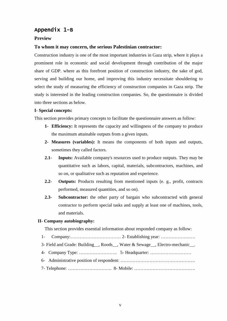
v
Appendix Appendix Appendix Appendix 1111----BBBB
Preview
To whom it may concern, the serious Palestinian contractor:
Construction industry is one of the most important industries in Gaza strip, where it plays a
prominent role in economic and social development through contribution of the major
share of GDP. where as this forefront position of construction industry, the sake of god,
serving and building our home, and improving this industry necessitate shouldering to
select the study of measuring the efficiency of construction companies in Gaza strip. The
study is interested in the leading construction companies. So, the questionnaire is divided
into three sections as below.
I- Special concepts:
This section provides primary concepts to facilitate the questionnaire answers as follow:
1- Efficiency: It represents the capacity and willingness of the company to produce
the maximum attainable outputs from a given inputs.
2- Measures (variables): It means the components of both inputs and outputs,
sometimes they called factors.
2.1- Inputs: Available company's resources used to produce outputs. They may be
quantitative such as labors, capital, materials, subcontractors, machines, and
so on, or qualitative such as reputation and experience.
2.2- Outputs: Products resulting from mentioned inputs (e. g., profit, contracts
performed, measured quantities, and so on).
2.3- Subcontractor: the other party of bargain who subcontracted with general
contractor to perform special tasks and supply at least one of machines, tools,
and materials.
II- Company autobiography:
This section provides essential information about responded company as follow:
1- Company:…………………………… 2- Establishing year: ……………….….
3- Field and Grade: Building__, Roods__, Water & Sewage__, Electro-mechanic__.
4- Company Type: ……………………. 5- Headquarter: ………………………
6- Administrative position of respondent: ………………………………………….
7- Telephone: ……………………….. 8- Mobile: ………………………………….

vi
III- Important evaluation of the measures of inputs and outputs:
This section aims to estimate the relative importance of the measures of inputs and
outputs from contractor's viewpoint. Please, identify (carefully) the relative importance of
the measures illustrated in the table according to the following criteria:
(1) not important. (2)some important. (3)medium important. (4)important. (5)very
important.
1. Input variables:
No Measures (1) (2) (3) (4) (5)
1 Labor: Skilled and unskilled workers, engineers,
supervisors, superintendents on sites (L).
2 Subcontractors (SUB).
3 Formal recorded capital (C).
4 Available cash flow (CF).
5 Used materials (M).
6 Machines, and equipments (EM).
7 Head office expenditure and overhead (HO).
8 Company's assets and properties (AS).
9 Company's age (A).
10 Energy and consumed materials (CM).
11 Company's experience (E).
12 Health and safety (HS).
13 Number of Employees at the head office (MS).
14 Company's reputation (R).
15 Geographical location of company (GL).

vii
2. Output variables:
No Measures (1) (2) (3) (4) (5)
1 Contractor's satisfaction in obtaining profit and
avoiding losses due to contract risks and claims (P).
2 Annual amount of contracts (CS).
3 Annual amount of contracts implemented (EW).
Do you think existence of any other measures? If yes mention them.
…………………………………………………………………………………………
Is there any tools used to measure companies' efficiency?
…………………………………………………………………………………………
Do you company have any willingness to participate in presenting the required data to
measure the efficiency of leading companies in Gaza strip? (Yes) ...…… (No) ………
With best regards.
The Researcher/ Younis Shoman
Mobile/ 0599------

viii
Appendix Appendix Appendix Appendix 1111----CCCC
Questionnaire Analysis:
I. inputs' Analysis
To analyze the questionnaire inputs shown in Appendix A, we used the factor analysis
approach which is provided by SPSS statistical software.
There are three stages in factor analysis:
1. First, a correlation matrix is generated for all variables. A correlation matrix is a
rectangular array of the correlation coefficients of the variables with each other.
2. Second, factors are extracted from the correlation matrix based on the correlation
coefficients of the variables.
3. Third, the factors are rotated in order to maximize the relationship between the
variables and some of the factors.
Several inputs and outputs variables were identified which influence the efficiency of
construction companies working at Gaza Strip. Where the questionnaire variables are
defined as follows:
•••• Respondents Position:
Measurement Level: ordinal.
Symbol Labels:
GC: Top management company's member (chairman, executive manager, or manager
assistant).
P.M: Project manager of construction company.
•••• Input Variables:
L, SUB, C, CF, M, EM, HO, AS, A, CM, E, HS, MS, R, GL.
•••• Output Variables:
P, CS, EW.
Measurement Levels: ordinal.
Labels Value:
(1) Not important. (2) Little important (3) Medium important.
(4) Important. (5) Very important.
Table (A1.1) shown the dataset of input variables. It illustrates the importance of the
variables as expressed by the respondents and the respondents positions.

ix
Table (A1.1): Input Dataset
Post L SUB C CF M EM HO AS CA CM E HS MS R GL GC 5 3 4 4 5 5 3 2 3 2 3 3 5 3 3 GC 4 5 4 5 5 2 2 4 2 3 4 2 4 2 4 GC 5 4 3 5 4 5 3 5 2 4 3 5 5 4 1 GC 5 5 4 4 5 4 1 2 4 4 4 3 4 4 3 GC 3 5 3 5 5 4 2 4 2 3 2 4 4 2 2 GC 5 4 4 3 5 5 3 3 5 2 5 2 5 5 3 GC 5 5 3 5 3 3 4 4 2 4 3 2 4 3 3 GC 5 4 3 3 5 5 3 3 4 3 3 4 4 4 2 GC 5 2 4 4 5 5 2 2 3 4 4 3 5 2 1 GC 4 5 3 5 4 4 1 4 2 4 2 2 4 4 3 GC 2 5 3 5 5 4 2 4 3 3 3 3 5 3 3 GC 5 4 2 3 5 4 3 3 4 4 3 5 4 3 2 GC 5 3 4 5 4 5 3 4 3 3 2 4 4 4 3 GC 3 5 3 4 5 4 2 2 4 5 4 3 4 3 2 GC 5 4 1 5 5 5 3 4 3 4 3 2 5 3 3 GC 4 5 4 4 5 4 1 3 4 3 4 3 4 4 1 GC 5 5 4 5 4 2 2 1 4 4 2 4 4 5 3 GC 5 4 3 5 5 5 2 4 2 3 4 3 5 3 2 GC 3 5 3 5 5 3 1 1 3 4 3 4 4 4 3 GC 5 4 2 2 5 5 3 2 5 3 4 5 5 4 3 GC 4 5 2 5 3 4 2 1 4 1 2 3 5 3 2 GC 5 3 4 4 5 5 2 4 3 3 4 4 5 4 2 GC 5 4 2 5 4 4 3 5 2 4 3 3 4 3 3 GC 5 4 2 3 5 5 1 3 4 2 4 4 4 4 2 GC 4 5 3 5 4 4 4 4 3 3 5 3 5 4 2 GC 5 5 3 3 5 1 2 3 4 4 3 4 4 5 3 GC 5 3 4 5 4 5 2 4 2 5 4 3 4 4 4 GC 5 4 2 4 5 4 3 2 3 4 1 2 2 2 3 GC 4 5 3 5 4 4 4 1 3 2 2 1 4 1 2 GC 5 3 4 5 5 5 2 4 2 3 3 2 3 2 4 GC 5 4 2 4 5 5 2 2 3 4 4 3 4 3 1 GC 3 5 3 5 4 3 1 4 1 4 2 2 4 2 3 PM 5 4 2 4 5 5 3 3 3 5 2 2 3 2 2 PM 5 4 2 5 4 4 2 4 2 4 1 1 3 2 2 PM 5 3 4 4 5 5 1 3 3 5 3 2 4 1 2 PM 5 4 1 5 4 4 2 4 2 3 2 3 4 2 1 PM 4 5 3 4 5 4 3 3 4 5 1 2 3 2 1 PM 5 4 2 4 5 5 4 3 4 2 2 2 2 3 3 PM 5 2 4 5 4 5 3 4 3 4 3 1 3 2 2 PM 4 5 1 4 5 2 2 3 4 5 2 3 4 2 4 PM 5 4 1 4 5 5 3 3 1 3 2 1 3 2 1 PM 5 5 3 5 4 3 1 2 2 4 3 2 4 1 2

x
Interpretation of input analysis results:
Descriptive Statistics
The first output of the analysis is Table (A1.2) of descriptive statistics for all the input
variables under investigation. Typically, the mean, standard deviation and number of
respondents (N) who participated in the survey are given. Looking at the mean, one can
conclude that material (M) is the most important variable because it has the most
important variable because it has the highest mean of 4.6.
Table (A1.2): Descriptive Statistics of Input Variables
Descriptive Statistics
4.55 .772 42
4.19 .862 42
2.88 .968 42
4.36 .791 42
4.60 .587 42
4.14 1.026 42
2.33 .902 42
3.10 1.078 42
3.00 .988 42
3.52 .969 42
2.93 1.022 42
2.83 1.080 42
4.02 .780 42
2.98 1.093 42
2.40 .885 42
L
SUB
C
CF
M
EM
HO
AS
CA
CM
E
HS
MS
R
GL
Mean Std. Deviation Analysis N
Factor Analysis
• The Correlation matrix
The next output from the analysis is the correlation coefficient shown in Table (A1.3). A
correlation matrix is simply a rectangular array of numbers which gives the correlation
coefficients between a single variable and every other variable in the investigation. The
correlation coefficient between a variable and itself is always 1, hence the principal
diagonal of the correlation matrix contains 1s. The correlation coefficients above and
below the principal diagonal are the same. The determinant of the correlation matrix is
shown at the foot of the table below.

xi
Table (A1.3):Correlation Matrix
Correlation Matrix
1.000-.564 -.041 -.288 -.037 .330 .257 .053 .064 -.002 .082 -.005 -.144 .103-.082
-.5641.000 -.235 .112 -.133 -.666 -.146-.204 .086 -.006 -.15 .035 .029 .108 .088
-.041-.235 1.000 .121 -.001 .018 -.205-.012 .051 -.010 .386 .051 .198 .228 .172
-.288 .112 .121 1.000 -.574 -.155 -.068 .303 -.687 .068 -.27 -.357 -.014 -.300 .102
-.037-.133 -.001 -.574 1.000 .179 -.154-.130 .337 .082 .235 .160 -.085 .023-.006
.330-.666 .018 -.155 .179 1.000 .237 .164 .000 -.224 .196 -.044 .057 -.040-.334
.257-.146 -.205 -.068 -.154 .237 1.000 .117 .110 -.205 -.11 -.117 -.116 -.016-.020
.053-.204 -.012 .303 -.130 .164 .1171.000 -.504 .138 .051 -.049 .026 .002 .086
.064 .086 .051 -.687 .337 .000 .110-.504 1.000 -.153 .242 .366 .127 .452 .028
-.002-.006 -.010 .068 .082 -.224 -.205 .138 -.153 1.000 -.13 -.054 -.243 -.172 .031
.082-.150 .386 -.270 .235 .196 -.106 .051 .242 -.134 1.00 .298 .583 .435 .033
-.005 .035 .051 -.357 .160 -.044 -.117-.049 .366 -.054 .298 1.000 .468 .596-.030
-.144 .029 .198 -.014 -.085 .057 -.116 .026 .127 -.243 .583 .468 1.000 .372-.050
.103 .108 .228 -.300 .023 -.040 -.016 .002 .452 -.172 .435 .596 .372 1.000 .187
-.082 .088 .172 .102 -.006 -.334 -.020 .086 .028 .031 .033 -.030 -.050 .1871.000
L
SU
B
C
CF
M
EM
HO
AS
CA
CM
E
HS
MS
R
GL
Correlation
L SUB C CF M EM HO AS CA CM E HS MS R GL
• Kaiser-Meyer-Olkin (KMO) and Bartlett's Test
The next item from the output is the Kaiser-Meyer-Olkin (KMO) and Bartlett's test
shown in Table (A1.4). The KMO measures the sampling adequacy which should be
greater than 0.5 for a satisfactory factor analysis to proceed. Looking at the table below,
the KMO measure is 0.547. From the same table, we can see that the Bartlett's test of
sphericity is significant. That is, its associated probability is less than 0.05. In fact, it is
actually 0.000. This means that the correlation matrix is not an identity matrix.
Table (A1.4): Kaiser-Meyer-Olkin (KMO) and Bartlett's Test
KMO and Bartlett's Test
.547
217.334
105
.000
Kaiser-Meyer-Olkin Measure of SamplingAdequacy.
Approx. Chi-Square
df
Sig.
Bartlett's Test ofSphericity

xii
• Communalities
The next item from the output is Table (A1.5) of communalities which shows how
much of the variance in the variables has been accounted for by the extracted factors.
For instance over 85.5% of the variance in CF is accounted for while 65.1% of the
variance in L is accounted for.
Table (A1.5): Communalities
Communalities
1.000 .651
1.000 .838
1.000 .779
1.000 .855
1.000 .685
1.000 .790
1.000 .669
1.000 .740
1.000 .824
1.000 .701
1.000 .698
1.000 .735
1.000 .778
1.000 .775
1.000 .732
L
SUB
C
CF
M
EM
HO
AS
CA
CM
E
HS
MS
R
GL
Initial Extraction
Extraction Method: Principal Component Analysis.
Extraction communalities are estimates of the variance in each variable accounted for by
the components. The communalities in this table are all high, which indicates that the
extracted components represent the variables well.
• Total Variance Explained
The next item shows in Table (A1.6) is all the factors extractable from the analysis along
with their Eigen values, the percent of variance attributable to each factor, and the
cumulative variance of the factor and the previous factors. Notice that the first factor

xiii
accounts for 21.304% of the variance, the second 15.829% , the third 13.032% ,the forth
9.441 ,the fifth 8.151 and the sixth 7.254 . All the remaining factors are not significant.
Table (A1.6): Total Variance Explained
Total Variance Explained
3.196 21.304 21.304 3.196 21.304 21.304 2.408 16.054 16.054
2.374 15.829 37.133 2.374 15.829 37.133 2.371 15.807 31.861
1.955 13.032 50.165 1.955 13.032 50.165 2.293 15.285 47.146
1.416 9.441 59.606 1.416 9.441 59.606 1.518 10.121 57.267
1.223 8.151 67.757 1.223 8.151 67.757 1.343 8.954 66.221
1.088 7.254 75.011 1.088 7.254 75.011 1.318 8.790 75.011
.889 5.926 80.937
.633 4.222 85.159
.581 3.876 89.035
.498 3.323 92.357
.372 2.477 94.835
.277 1.848 96.682
.199 1.328 98.010
.161 1.071 99.081
.138 .919 100.000
Component
1
2
3
4
5
6
7
8
9
10
11
12
13
14
15
Total
% of
Variance
Cumulative
% Total
% of
Variance
Cumulative
% Total
% of
Variance
Cumulative
%
Initial Eigenvalues
Extraction Sums of Squared
Loadings
Rotation Sums of Squared
Loadings
Extraction Method: Principal Component Analysis.
the table shows the extracted components. They explain nearly 75% of the variability in
the original fifteen variables, so you can considerably reduce the complexity of the data
set by using these components, with only a 25% loss of information.
Scree Plot
The Scree plot is a graph of the Eigen values against all the factors shown in Figure
(A1.1). The graph is useful for determining how many factors to retain. The point of
interest is where the curve starts to flatten. It can be seen that the curve begins to flatten
between factors 6 and 7. Note also that factor 7 has an Eigen value of less than 1, so only
six factors have been retained. The selected factors were M, L, CF, SUB, EM, and MS.

xiv
The scree plot helps to determine the optimal number of components. The Eigen value of
each component in the initial solution is plotted.
151413121110987654321
Component Number
3
2
1
0
Eigenvalue
0.140.160.20.28
0.37
0.50.58
0.63
0.89
1.09
1.22
1.42
1.95
2.37
3.2
Scree Plot
Figure (A1.1): Scree Plot of the Input Variables
• Component (Factor) Matrix
Table (A1.7) shows the loadings of the fifteen variables on the six factors extracted. The
higher the absolute value of the loading, the more the factor contributes to the variable.
The gap on the Table represent loadings that are less than 0.5, this makes reading the
Table easier. We suppressed all loadings less than 0.5.

xv
Table (A1.7): Component Matrix
Component Matrixa
-.679
.823
.516 -.535
-.713 .536
.542
-.802
-.600
.555 .508
.734
.625
.671
.673
.512 .558
.699
.734
L
SUB
C
CF
M
EM
HO
AS
CA
CM
E
HS
MS
R
GL
1 2 3 4 5 6
Component
Extraction Method: Principal Component Analysis.
6 components extracted.a.
• Rotated Component (Factor) Matrix
The idea of rotation is to reduce the number factors on which the variables under
investigation have high loadings. Rotation does not actually change anything but makes
the interpretation of the analysis easier. Looking at Table (A1.8), we can see that GL is
substantially loaded on Factor (Component) 6 , CM is substantially loaded on Factor 5, C
and E are substantially loaded on Factor 4, L, SUB and EM are substantially loaded on
Factor 3, while CF, M, AS and CA are substantially loaded on Factor 2 . All remaining
variables are substantially loaded on Factor1. These factors can be used as variables for
further analysis.

xvi
Table (A1.8): Rotated Component Matrix
Rotated Component Matrixa
.768
-.857
.831
-.821
.640
.719
-.689
.818
.807
.604 .526
.814
.729
.776
.831
L
SUB
C
CF
M
EM
HO
AS
CA
CM
E
HS
MS
R
GL
1 2 3 4 5 6
Component
Extraction Method: Principal Component Analysis.
Rotation Method: Varimax with Kaiser Normalization.
Rotation converged in 8 iterations.a.
Comment:
According to the factor analysis, there are six significant inputs which are L ,SUB, ,CF
,M ,EM and MS.
•••• Output Variables:
P, CS, EW.
Measurement Levels: ordinal.
Labels Value:
(2) Not important. (2) Little important (3) Medium important.
(5) Important. (5) Very important.
Table (A1.9) shown the dataset of output variables. It illustrates the importance of the
variables as expressed by the respondents and the respondents positions.

xvii
Table (A1.9): Output Dataset Post P CS EW GC 5 3 5 GC 3 4 3 GC 5 5 5 GC 4 2 4 GC 5 3 5 GC 4 4 5 GC 5 2 5 GC 4 3 3 GC 4 4 4 GC 5 3 5 GC 5 1 5 GC 4 2 4 GC 5 4 5 GC 4 3 4 GC 5 3 5 GC 4 4 4 GC 5 2 4 GC 5 2 5 GC 4 3 5 GC 4 5 4 GC 5 4 5 GC 4 2 4 GC 5 1 5 GC 4 3 2 GC 5 3 5 GC 5 2 4 GC 4 2 4 GC 5 1 5 GC 5 2 5 GC 4 5 3 GC 5 4 4 GC 4 2 4 PM 5 1 5 PM 5 3 4 PM 5 1 5 PM 4 4 3 PM 5 2 4 PM 4 1 2 PM 5 2 4 PM 4 1 2 PM 5 3 5 PM 4 2 3

xviii
I. Outputs' Analysis:
To analyze the questionnaire outputs shown in Appendix (1-B), we used the factor
analysis approach which is provided by SPSS statistical software.
Interpretation of Output analysis results:
• Descriptive Statistics
The first output from the analysis is Table (A1.10) of descriptive statistics for all the
variables under investigation. Typically, the mean, standard deviation and number of
respondents (N) who participated in the survey are given. Looking at the mean, one can
conclude that gained profit (P) is the most important variable because it has the highest
mean of 4.52.
Table (A1.10): Descriptive Analysis
Descriptive Statistics
4.52 .552 42
2.69 1.179 42
4.19 .917 42
P
CS
EW
Mean Std. Deviation Analysis N
• The Correlation matrix
The next output from the analysis is the correlation coefficient shown in Table (A1.11). A
correlation matrix is simply a rectangular array of numbers which gives the correlation
coefficients between a single variable and every other variable in the investigation. The
correlation coefficient between a variable and itself is always 1, hence the principal
diagonal of the correlation matrix contains 1s. The correlation coefficients above and
below the principal diagonal are the same. The determinant of the correlation matrix is
shown at the foot of the table below.

xix
Table (A1.11): Correlation Matrix
Correlation Matrix
1.000 -.232 .666
-.232 1.000 -.012
.666 -.012 1.000
P
CS
EW
CorrelationP CS EW
• Kaiser-Meyer-Olkin (KMO) and Bartlett's Test
The next item from the output is the Kaiser-Meyer-Olkin (KMO) and Bartlett's test
shown in Table (A1.12). The KMO measures the sampling adequacy which should be
greater than 0.5 for a satisfactory factor analysis to proceed. Looking at the table below,
the KMO measure is 0.456. From the same table, we can see that the Bartlett's test of
sphericity is significant. That is, its associated probability is less than 0.05. In fact, it is
actually 0.000. This means that the correlation matrix is not an identity matrix.
Table (A1.12): Kaiser-Meyer-Olkin (KMO) and Bartlett's Test
KMO and Bartlett's Test
.456
26.662
3
.000
Kaiser-Meyer-Olkin Measure of SamplingAdequacy.
Approx. Chi-Square
df
Sig.
Bartlett's Test ofSphericity
• Communalities
The next item from the output is Table (A1.13) of communalities which shows how much
of the variance in the variables has been accounted for by the extracted factors. For
instance 85% of the variance in gained profit is accounted for while 10% of the variance
in contracts (CS) is accounted for.
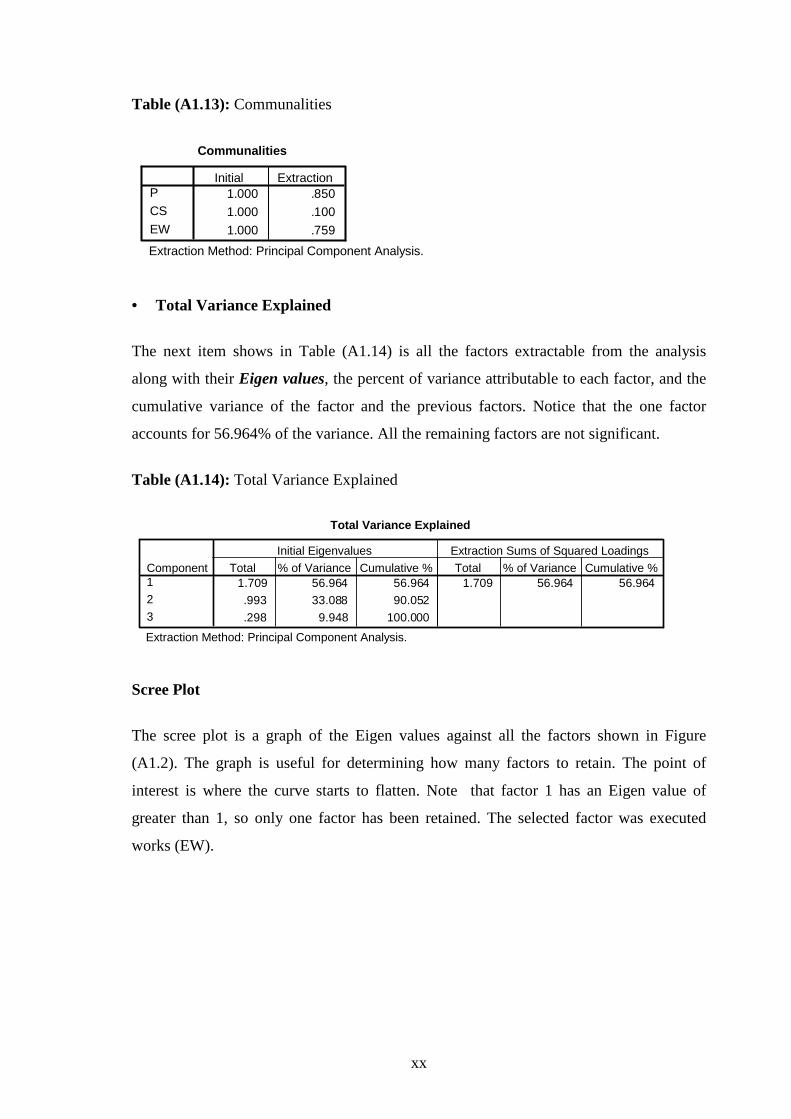
xx
Table (A1.13): Communalities
Communalities
1.000 .850
1.000 .100
1.000 .759
P
CS
EW
Initial Extraction
Extraction Method: Principal Component Analysis.
• Total Variance Explained
The next item shows in Table (A1.14) is all the factors extractable from the analysis
along with their Eigen values, the percent of variance attributable to each factor, and the
cumulative variance of the factor and the previous factors. Notice that the one factor
accounts for 56.964% of the variance. All the remaining factors are not significant.
Table (A1.14): Total Variance Explained
Total Variance Explained
1.709 56.964 56.964 1.709 56.964 56.964
.993 33.088 90.052
.298 9.948 100.000
Component1
2
3
Total % of Variance Cumulative % Total % of Variance Cumulative %
Initial Eigenvalues Extraction Sums of Squared Loadings
Extraction Method: Principal Component Analysis.
Scree Plot
The scree plot is a graph of the Eigen values against all the factors shown in Figure
(A1.2). The graph is useful for determining how many factors to retain. The point of
interest is where the curve starts to flatten. Note that factor 1 has an Eigen value of
greater than 1, so only one factor has been retained. The selected factor was executed
works (EW).

xxi
321
Component Number
1.75
1.50
1.25
1.00
0.75
0.50
0.25
Eigenvalue
0.298
0.993
1.709
Scree Plot
Figure (A1.2): Scree Plot of Output Variables
• Component (Factor) Matrix
Table (A1.15) shows the loadings of the three variables on the one factor extracted. The
higher the absolute value of the loading, the more the factor contributes to the variable.
The gap on the table represent loadings that are less than 0.5, this makes reading the
Table easier. We suppressed all loadings less than 0.5.

xxii
Table (A1.15): Component Matrix
Rotated Component (Factor) Matrix
The idea of rotation is to reduce the number factors on which the variables under
investigation have high loadings. Rotation does not actually change anything but makes
the interpretation of the analysis easier. Looking at the table below, we can see that there
is only one significant component which is P .
Rotated Component Matrix a
Only one component was extracted.The solution cannot be rotated.
a.
Comment:
According to the factor analysis, there is one significant output which is gained profit (P).

xxiii
Appendix Appendix Appendix Appendix 2222 Appendix Appendix Appendix Appendix 2222----AAAA
Arabic Version
���W �Eدرا ا��4"�م: �أ.� ا����� -�W^ و� �� %�آ
�B� �4 أو Qو � :، و=1،،،،،،،،،،،،،،،،،،،،، أ��0+ '(�� ا6R@م ا�=,� fأو +�Q�� ء 1/+، اw��'6 ��+ آ) /= �� ا�1gق وا��� �'��� ��`�6'+ ا�'� b ، وأ<#1ادك +� ء أ/1 � أن ، ور
ع E#Xة ا�#Gي ��'#�� �Eو��1##!� ح ه#Gا ا��#�وع ا�B$�#� وا��# م ���# و�� #C� �#� � ه�#� /J و�'+ و<�1ك /#��!=�
�B'آ�_ J� �8 A ت � �$� �� ا�� رآ� �� ا��$��� ��B'$X2 ر� ةLا��ا ���ع �س آ'�ءة %�آ�ت ا�"! � � ���ة ��
� وا�'� � ر/�'Aا ��� ��J ا�آ J/ (��� a$� ت ��6 ، /J ا��آ�'� ( R �/ت ا�@ز � ح ا�1gق وا�1�� �� ا�$�C� اG#ه
ءات وا��آ ت ا�= /�� �� ه#Gا ا�Gي 6 ا�B$�� ��وعا��Rع ا !� ���!� �� � رN ا��#�� ر ا�#Gي #6 �� ه#�b ن�%!�'
،tا �v�� ن وا�#���� و�#J �#�'?1م إf ��&#�ض ا�=��#� ا��(#1د �#� ه#Gا �'Bا� �Q ن�B'6 ت � ن آ �� ا�$� �B�1وا�
� ت ا��!��� �$� 6 ه� وأ/�1 J/ (B� ) /��8ل�ECا� �Bوا� Vا�$(.
� Eرا ��(ت ا�� F -�'@: ت و�=$J/ (/s� �v آ �� ا�ARة ��اءة � :ا�' ��� ا��@0, ت /U /�ا� ةB) د�� و/������ ا�$�
��ا�#U ا��# ر�J�#61��/ J#/ U و���#� : J��I<�ت ا�_��4� -١ J��/ �G+ آ �� ا�<#�ر وا����$# ت ا���#���1 ��=# 1gو��
و�� ل وK�@A وأي �=��#� ت أو �#@ج �=#�د � J��/ ��1# ا��$ _#�ة ��#2 ا�=#� - �#@ج -أ<#�ر .(�#�آ� ��#) ا �#U ا��
). /�و ت-و<$ ت
ول ا�$# JQ ه#� ا��C#� ا�'#� � / :Subcontractors)( ���و�� ا���=> -٢#� G#�%�� 2#�� �/�#�=ول ا� ا���##�=/ 1#� ='
.و��ر�1 ا���اد وا��=1ات �{�� ل ا����ط �NG ا�G�%�� ��Cه
ت وا��=1ات ا�����: Equipments and Machines) ( ا�4_ ات وا`� �ت-٣��Pا ���� <#1ول -آ#� ��#�آ� وه�
�� ).٧(ر
#� ��#2 �#�?� أA#�ى � رJ#/ �#X ذات ا��ر�#� /#U ا�$�# ن -٤ 'Bا� JB��#� ،ت #� 0 �� �1م آ% �� أي /J ا�1Cاول ��$� ��
�� /�(: ��1Cول ر��s �� أوراق ا�( �� ا�1را��6) آGا(B �� .وإ�(
٥- �� �'#� ،�#B��/ر ا�fف ا�#1و@#A �/1?'�#ل آ�ن ا�=�@ت ا�� 0 �� �#B��/ر ا�f1و#� ت ا�C#1اول #� � �#� � آ�#�
.d�0 6=� ا��gف ا��='�1 ���ق ��J/E ا��(1د
:ا�B �ة ا�Aا@ � �!�آ�: أو(
........................................: ��6 ا�'F�6s-٢ ................................................................: ا6� ا��آ�-١
٣-g� آ��ا� y��.......................................................... ل-٤ Cا�� :....................................................
.......................: ا���� ا������ ���آ�-٦.............................................................. : ��ع ا��آ�-٥
ت-٧� ......................................................................................: ا���آE اRداري ��J ���م '=$�v ا�$�

xxiv
B) د�� و/�������� ذجا��< ء �=$�v ا� �8 �: ا��آ� ا�?bف وو�Bا� U� اJ/ ���P وا
درا��W �E�(آ� .7ت و��:�ت ا�!� �� , �<�ت � -أ
��: ا�4 .7ت) ا١(: ول "B4در ا��a4ا�
b ���"ا�$ ٢٠٠٢ ٢٠٠٣ ٢٠٠٤ ٢٠٠٥ ٢٠٠٦
ةWIا�4"5 � ا� �� ر
$ J�61ا���� @/ _ �� ���ا�Uا�=� . ١ ت ا�����آ� ���آ� $ ��Pا��=1ات وا. ٢ ���� ا���اد ا���'?1/� $ . ٣ �ا������ ا����1 $ ٤ ��d'B ا������ �1د J��/ ٥ ا���J�%c ا�= $ JQ ٦ /� و�� ا�$
� 4� ا��4Rل ا��Pf4ة(ا�4�:�ت ) ب١(: ول :(
b ���"ا�$ ٢٠٠٢ ٢٠٠٣ ٢٠٠٤ ٢٠٠٥ ٢٠٠٦
ةWIا�4"5 � ا� �� ر
$ ��� ر�U أ/ ١ ر��Q Uق $ / ٢ $ �/ Uر� /Nري C/٣ و $ +�� B�/آ��و Uر� / ٤ ٥ أ�� ل أ�Aى $ $ �� �>Rا
.7ت ا�!�آ�-ب�
� ا��4Rل ا�A'f4ة �> ) ٢(: ول � �� "B4اد ا�I44� ا� �)١/١/٢٠٠٢ ( S"W)٣١/١٢/٢٠٠٦ ( �'$ا�"� ا�HEI"4 ا�IfBي
$ ٢٠٠٢ ٢٠٠٣ ٢٠٠٤ ٢٠٠٥ ٢٠٠٦ b-Iا�
ا�I4اد �� "B4ا�
ول:) ٣ ( <� F4_ا� X� �� ,I4ا"B4ا�_��4� ا� b ���@)) ١/١/٢٠٠٢ S"W٣١/١٢/٢٠٠٦(( b ���"ا�$ HEI"4ا�
$ا�IfBي ٢٠٠٢ ٢٠٠٣ ٢٠٠٤ ٢٠٠٥ ٢٠٠٦ b-Iا� �� ر
Uر� ./1راء / ١ J�61��/. ٢ J���� ،J�$� J�0، /�ا�/... ٣ �� دا��� �� . ٤ `/ �� ���'�. ٥ ��� .أ<�ر إ� ٦ �� �>Rا

xxv
�� ا�I"4��ة �!�آ� �> ) ٤(: ول �fا� ��I B4� ا� �)١/١/٢٠٠٢ ( S"W)٣١/١٢/٢٠٠٦(
�'$ا�"� ا�HEI"4 ا�IfBي
$ ٢٠٠٢ ٢٠٠٣ ٢٠٠٤ ٢٠٠٥ ٢٠٠٦ b-Iا�
��I B4� ا� � �� �fا�$
�� ���و�� ا���=> �>ا� �_�ت ا�B4"��� وا��Pر�) ٥(: ول EاI, ةA'f4�4ل ا�R4� ا� � �١/١/٢٠٠٢ S"W
٣١/١٢/٢٠٠٦ $ا� �_� ا�B4"��� ا�"�ر� j��iW7ت / أ,f �: ا��P4ل
...=�ق � 4� ا�_�$ �R ��ر
ا���=>�� ر
/ / ١
/ / ٢
/ / ٣
/ / ٤
/ / ٥
/ / ٦
/ / ٧
/ / ٨
/ / ٩
/ / ١٠
/ / ١١
/ / ١٢
/ / ١٣
/ / ١٤
/ / ١٥
/ / ١٦
/ / ١٧
/ / ١٨
/ / ١٩
/ / ٢٠
!�آ� �> � 4� ا�4_ ات وا`� �ت ا�44Iآ� �) ٦(: ول )) ١/١/٢٠٠٢ S"W٣١/١٢/٢٠٠٦((
$ا�� 4� HEI"4ا� $ا�IfBي ٢٠٠٢ ٢٠٠٣ ٢٠٠٤ ٢٠٠٥ ٢٠٠٦
b-Iا� FBB�
١ ٢ ٣ ٤ ٥ ٦
���4:lا

xxvi
ول :)٧(�B L�4"^ ا����, < د ا�nI4' > ا�_��R <� )) ١/١/٢٠٠٢ S"W٣١/١٢/٢٠٠٦(( �'$ا�"� ا�HEI"4 ا�IfBي
$ ٢٠٠٢ ٢٠٠٣ ٢٠٠٤ ٢٠٠٥ ٢٠٠٦ b-Iا�
< 'nI4د ا� R
��:�ت ا�!�آ�-ج
S"W٣١/١٢/٢٠٠٦ ١/١/٢٠٠٢ا� �_�ت ا�B4"��� وا��Pر�� ��4Rqل ا�A'f4ة �>) ٨(: ول $ا� �_� ا�B4"��� ا�"�ر� j��iW7ت ...=�ق / أ,f �: ا��P4ل � 4� ا�_�$ ر�� ا�_ � �� ر
/ / ١
/ / ٢
/ / ٣
/ / ٤
/ / ٥
/ / ٦
/ / ٧
/ / ٨
/ / ٩
/ / ١٠
/ / ١١
/ / ١٢
/ / ١٣
/ / ١٤
/ / ١٥
/ / ١٦
/ / ١٧
/ / ١٨
/ / ١٩
/ / ٢٠
/ / ٢٠
/ / ٢١
/ / ٢٢
/ / ٢٣
/ / ٢٤
�Wوأ= ^ @� �ت ا��� �=�R X� ---- --- --:Iال

xxvii
Appendix Appendix Appendix Appendix 2222----BBBB
Case Study
To whom it may concern, the serious Palestinian contractor:
Inciting first, all the meanings of honesty and belonging to your home, then to your
company which is built by your toil, to give us point of time and effort to achieve a
success of our research of measuring the efficiency of leading construction companies in
Gaza strip. The research depending on a needed data about your company. The selection
of your company among numerous companies depend on your desire and the company
abilities. Sought success of the research is usefulness for construction sector and
construction companies. All given data will be kept top secret and the use of it only is
limited for scientific research.
Details of study:
Please, carefully fill required data taking into account the following definitions.
1- Manpower expenditure: it includes fees, wages, compensations, and physical
therapy paid out for engineers, supervisors, superintendents, and labors.
2- Subcontractors: is the other party who contracts with the construction company to
supply materials or/and equipments or/and machines to perform assigned works.
3- Equipments and Machines: it is the value of equipments and machines possessed
by the company.
4- In case of any inadequacy of data tables, you may write in another blank table
copy with reference to it as a supplementary for table number.
5- In case of currency used other than US $, then it may required to evaluate all the
data tables by US $ exchange rate in the market for specified time.
I- Company autobiography:
2- Company: …………………………………. 2- Establishing year: ……………….
3- Field and Grade: Building__, Roods__, Water & Sewage__, Electro-mechanic__.
4- Company Type: ……………………. 5- Headquarter: ………………………
6- Administrative position of respondent: ………………………………………….
7- Telephone: ……………………….. 8- Mobile: ………………………………….

xxviii
A- Summary of the Company's Inputs and Output Data (Case Study)
Form (1) Input Variables: Years No. Variable Unit
2002 2003 2004 2005 2006 1 Labors Cost. $ 2 Equipment & Machines. $ 3 Materials. $ 4 Cash Flow. $ 5 Head office's employees No 6 Subcontractors $
Form (2) Output Variables: Years No. Variable Unit
2002 2003 2004 2005 2006 1 Buildings. $ 2 Roads. $ 3 Water & Sewage. $ 4 Electromechanical. $ 5 Sundries. $
Total $
B- The Company's Inputs Form (3) Cost of used materials (1/1/2002 -31/12/2006)
Cost of used materials $ Description 2002 2003 2004 2005 2006
Average per year
Used materials for projects. Form (4) Labors expenditures (1/1/2002 – 31/12/2006)
Expenditure $ No. Description of expenditure 2002 2003 2004 2005 2006
Average per year
1 Project managers. 2 Engineers. 3 Surveyors, foremen,
technicians,
4 Permanently labors. 5 Temporary labors. 6 Additional fees (if in). Total

xxix
Form (5) Cash flow possessed (1/1/2002 – 31/12/2006) Cash flow $ Description
2002 2003 2004 2005 2006 Average per year
Possessed cash flow. Form (6) Amount of executed works by subcontractors (1/1/2002 -31/12/2006) No. Subcontr-
act No. Subcontract Amount $
Field (buildings, roads, …)
Date Payable payment $
Notes
1 / / 2 / / 3 / / 4 / / 5 / / 6 / / 7 / / 8 / / 9 / / 10 / / 11 / / 12 / / 13 / / 14 / / 15 / / 16 / / 17 / / 18 / / 19 / / 20 / /
Form (7) Value of possessed equipments and machines (1/1/2002 – 31/12/2006) Value $ No. Equipments &
Machines Value 2002 2003 2004 2005 2006 Average per year
1 2 3 4 5 6
Total

xxx
Form (8) Number of head office staff (1/1/2002 – 31/12/2006) Expenditure $ Description
2002 2003 2004 2005 2006 Average per year
No. of head office employees.
C- The Company's Outputs
Table (8) Payable interim and final payments in return of executed works (1/1/2002 -31/12/2006) No. Contract
No. Contract Amount $
Field (buildings, roads, …)
Payable payment $
Date Notes
1 / / 2 / / 3 / / 4 / / 5 / / 6 / / 7 / / 8 / / 9 / / 10 / / 11 / / 12 / / 13 / / 14 / / 15 / / 16 / / 17 / / 18 / / 19 / / 20 / / 21 / / 22 / / 23 / / 24 / /
With researcher best wishes
Mobile --------

xxxi
Appendix Appendix Appendix Appendix 3333
Appendix Appendix Appendix Appendix 3333----AAAA
3-A Correlation Matrix between Executed Works and Efficiency Scores
EW Efficiency
Correlation EW 1 0.215
Efficiency 0.215 1

xxxii
Appendix Appendix Appendix Appendix 3333----BBBB
0
500
1000
1500
2000
2500
3000
3500
4000
1 2 3 4 5 6
Inefficient DMUs
Mat
eria
ls C
ost i
n $1
000
١�������
٢�������
C4 C9 C11 C13 C21 C22
TargetActual
Figure (A3.1): Comparison between Target and Actual Materials Cost of Inefficient DMUs.
0
100
200
300
400
500
600
1 2 3 4 5 6
Inefficiet DMUs
Labo
r C
ost i
n $1
000
١�������
٢�������
TargetActual
C4 C9 C11 C13 C21 C22
Figure (A3.2): Comparison between Target and Actual Labor Cost of Inefficient DMUs.

xxxiii
0
50
100
150
200
250
1 2 3 4 5 6
Inefficiet DMUs
Cas
h F
low
in $
1000
١�������
٢�������
TargetActual
C4 C9 C11 C13 C21 C22
Figure (A3.3): Comparison between Target and Actual Cash Flow of Inefficient DMUs.
0
500
1000
1500
2000
2500
1 2 3 4 5 6
Inefficiet DMUs
Sub
cont
ract
or C
ost i
n $1
000
١�������
٢�������
TargetActual
C4 C9 C11 C13 C21 C22
Figure (A3.4): Comparison between Target and Actual Labor Cost of Inefficient DMUs.

xxxiv
0
500
1000
1500
2000
2500
1 2 3 4 5 6
Inefficiet DMUs
Equ
ipm
ent &
Mac
hine
s V
alue
in $
1000
١�������
٢�������
TargetActual
C4 C9 C11 C13 C21 C22
Figure (A3.5): Comparison between Target and Actual Machines value of Inefficient DMUs.
0
5
10
15
20
25
30
1 2 3 4 5 6
Inefficiet DMUs
Man
gem
ent S
taff
١�������
٢�������
C4 C9 C11 C13 C21 C22
Figure (A3.6): Comparison between Target and Actual Management Staff of Inefficient DMUs.

xxxv
Appendix Appendix Appendix Appendix 3333----CCCC
Table (A3.1): CCR Variables Weights of the Year 2002
DMU Score WI1 WI2 WI3 WI4 WI5 WI6 C1 0 0 0 0 0 0 0.1 C2 100 3.9E-06 1.2E-06 0 0 4.52E-06 0 C3 83.70% 8.8E-07 1.1E-06 0 5.7E-06 0 0 C4 100 2.2E-06 0 0 2.6E-06 0 0.003378 C5 100 0 0 0 0 0 0 C6 100 0 0 0 7.7E-05 0.0001 0 C7 100 9E-07 0 0 3.2E-07 7E-08 0.005313 C8 81.2 5.5E-07 8.3E-07 0 2.3E-07 0 0 C9 100 6.7E-07 0 7.1E-07 0 1.7E-07 0.000153
C10 100 4.8E-06 0 0 8.7E-07 5.36E-06 0 C11 99.7 2.1E-05 0 0 0 0 0 C12 100 0 0 0 0 0 0.25 C13 92.2 5.3E-07 3E-08 5.7E-07 9E-08 0 0 C14 100 0 0 2.9E-05 6.3E-05 0 0 C15 100 4.5E-07 1.1E-06 0 0 0 0 C16 82.3 1.6E-06 1.4E-07 0 0 2.02E-06 0.00565 C17 * * * * * * * C18 93.1 8.2E-06 1E-05 0 5.3E-05 0 0 C19 99.1 7.9E-07 1.4E-07 7.4E-07 0 2.3E-07 0 C20 99.8 3.3E-07 6E-08 3.1E-07 0 9E-08 0 C21 87.5 1.5E-06 0 1.5E-06 3.6E-07 0 0 C22 100 0 0 6.3E-07 0 0 0.140796
Total Weight 4.787E-05 1.482E-05 3.307E-05 2.0412E-04 1.1246E-04 0.50529 Average Weight 2.2795E-06 7.0571E-07 1.5748E-06 9.72E-6 5.3552E-06 0.02406143
* Data about this Company was Unavailable
Table (A3.2): CCR Variables Weights of the Year 2003
DMU Score WI1 WI2 WI3 WI4 WI5 WI6 C1 100% 1.7E-06 0 5.2E-07 1.17E-05 0 0 C2 97.40% 2E-06 0 0 2.8E-07 5.6E-06 0 C3 100% 0 9.3E-06 0 6.24E-06 8.3E-06 0 C4 66.70% 1.4E-06 6.5E-07 0 8.23E-06 0 0 C5 100% 0 0 0 0 0 0 C6 100% 2.6E-06 0 0 2.91E-05 5.5E-05 1E-08 C7 74.90% 3.1E-07 1E-07 0 2E-08 1.2E-06 0.009619 C8 0.00% 0 0 0 0 0 0.1 C9 98.80% 7.4E-07 1.1E-07 0 5.9E-07 2.7E-06 0
C10 96.70% 3.5E-06 0 0 1.42E-06 1.1E-05 0 C11 100% 9.7E-07 0 0 1.2E-07 3.4E-06 0.017281 C12 100% 0 0 0 0 6.4E-07 0.18474 C13 100% 0 6.7E-07 1.9E-07 2.9E-07 0 0.01666 C14 100% 0 2.4E-06 5.74E-06 2.95E-05 0 0 C15 100% 0 1E-05 0 0 0 1E-08 C16 81.90% 1.2E-06 1.9E-06 0 2.71E-06 6.7E-06 0 C17 * * * * * * * C18 100% 0 0 0 1.4E-05 0 0.2 C19 100% 0 5.4E-06 7.96E-06 0 1E-05 0 C20 100% 0 3E-06 0 0 6.7E-07 0.018541 C21 58.00% 1.2E-06 0 0 1.6E-07 3.3E-06 0 C22 100% 1.2E-06 0 2.3E-07 0 3.1E-06 0
Total Weight 1.672E-05 3.371E-05 1.464E-05 1.043E-04 1.11E-04 0.54684148 Average Weight 7.9619E-07 1.6052E-06 6.9714E-07 4.9652E-06 5.2914E-06 0.02604007
* Data about this Company was Unavailable.

xxxvi
Table (A3.3): CCR Variables Weights of the Year 2004
DMU Score WI1 WI2 WI3 WI4 WI5 WI6 C1 100% 4.3E-06 0 2.3E-06 2.33E-05 0 0 C2 83.10% 6.9E-07 2.3E-06 0 8E-07 6E-07 0.043292 C3 100% 0 1E-05 8E-07 1.32E-06 6E-08 0 C4 98.70% 9.4E-07 0 5.7E-07 3.22E-06 0 0.009226 C5 100% 0 0 0 0 0 0 C6 100% 2.1E-06 0 0 6.66E-06 5.6E-06 0.016947 C7 100% 3.4E-07 1.1E-06 1E-08 4E-07 0 0.022391 C8 100% 1.1E-06 6.5E-06 0 1.14E-06 0 0 C9 100% 1.8E-06 5E-08 1.1E-06 9E-07 7.5E-07 0
C10 87.80% 1.7E-06 5.3E-06 0 2.19E-06 2E-05 0 C11 90.50% 1.1E-06 0 0 3.5E-07 2.4E-07 0.045688 C12 100% 0 0 0 0 0 0.2 C13 94.70% 1.5E-07 5.4E-07 1.4E-07 1.9E-07 0 0.009665 C14 100% 0 0 3.6E-05 2.25E-05 0 0 C15 100% 0 1.6E-06 0 0 0 0.069914 C16 100% 0 0 1E-06 1.37E-05 3.8E-06 0.129004 C17 * * * * * * * C18 100% 1.2E-06 0 0 3.63E-06 0 0.031582 C19 100% 0 7E-06 9.7E-06 0 2.4E-05 0 C20 100% 9E-08 1.7E-06 2.2E-06 0 0 0.017564 C21 80.40% 6.6E-07 2.4E-06 6.4E-07 8.5E-07 0 0.043256 C22 100% 1.9E-06 0 0 0 0 0.018784
Total Weight 1.796E-05 3.867E-05 5.408E-05 8.11E-05 5.512E-05 0.65731223 Average Weight 8.1636E-07 1.7577E-06 2.4582E-06 3.6864E-06 2.5055E-06 0.02987783
* Data about this Company was Unavailable.
Table (A3.4): CCR Variables Weights of the Year 2005
DMU Score WI1 WI2 WI3 WI4 WI5 WI6 C1 100% 1.2E-05 0 4.2E-06 6.62E-05 0 0 C2 100% 0 2.9E-06 1.9E-07 0 8.7E-06 0.026886 C3 100% 0 1.5E-05 0 1.85E-06 3.2E-05 0 C4 100% 4.2E-07 0 1.1E-07 9.5E-07 0 0.004778 C5 100% 0 0 0 0 0 0 C6 100% 0 0 0 2.98E-05 4.9E-05 0.002059 C7 100% 5.4E-07 1E-07 0 3.5E-07 0 0.010607 C8 98.60% 0 6.8E-06 0 5.3E-07 1.7E-07 0.014396 C9 89.50% 2E-08 9E-07 3.1E-07 4.6E-07 0 0.036471
C10 96.40% 2.6E-06 1.9E-06 0 2.03E-06 5.4E-06 0 C11 88.00% 1.7E-06 1E-06 0 1.21E-06 3.5E-06 0 C12 100% 0 0 0 0 0 0.199999 C13 81.70% 0 6.1E-07 1.1E-07 1.9E-07 0 0.017734 C14 100% 0 1.5E-05 1.4E-05 0.000132 0 0 C15 100% 0 9.3E-06 0 0 0 1E-08 C16 100% 0 4.1E-06 0 1.53E-06 1.1E-05 0.050298 C17 92.30% 6.4E-06 0 0 2.01E-06 0 0 C18 100% 1.5E-06 0 0 1.38E-05 0 0.061843 C19 100% 0 3.5E-06 1.1E-05 0 6.4E-06 0 C20 100% 0 3.3E-06 1.4E-07 0 7.7E-07 0.023481 C21 78.80% 1.3E-06 4E-06 6.8E-07 9.3E-07 0 0 C22 100% 1.6E-06 0 3.2E-06 0 0 0
Total Weight 2.788E-05 6.836E-05 3.387E-05 2.543E-04 1.171E-04 0.44855152 Average Weight 1.2673E-06 3.1073E-06 1.5396E-06 1.1557E-05 5.3241E-06 0.02038871

xxxvii
Table (A3.5): CCR Variables Weights of the Year 2006
DMU Score WI1 WI2 WI3 WI4 WI5 WI6
C1 100% 1E-06 0 0 1.37E-06 1.4E-06 0.003668 C2 100% 0 1.4E-06 1.7E-06 0 2.2E-07 0.096816 C3 100% 0 6.3E-06 1.8E-05 3.21E-06 0 0 C4 93.89% 2.6E-06 5.8E-07 0 0.000001 0 0.007564 C5 100% 0 0 0 0 0 0 C6 100% 0 8.8E-07 0 7.82E-06 6.1E-06 0.080798 C7 100% 3.1E-07 2.1E-07 2E-07 4.7E-07 0 0.011887 C8 100% 0 9.2E-06 0 1.9E-07 3.9E-07 0 C9 90.40% 3.2E-07 1.9E-07 6.8E-07 3E-07 0 0.003342
C10 100% 2.9E-06 1.6E-06 0 2.43E-06 9.4E-06 0 C11 90% 3.5E-05 3.7E-06 0 1.02E-05 0 0 C12 100% 0 0 0 0 0 0.166667 C13 91.30% 1.1E-07 4.8E-07 1.8E-07 9E-08 0 0.005861 C14 100% 0 0 1.9E-05 5.99E-05 0 0 C15 100% 6E-08 8.8E-06 0 0 0 0 C16 100% 0 1.3E-05 0 2.03E-05 0 0 C17 100% 0 2.3E-06 0 1.31E-06 0 0.079135 C18 100% 0 8.6E-07 0 1.21E-05 0 0.159593 C19 100% 6E-07 1.5E-06 7.7E-06 0 0 0 C20 100% 6E-08 2.8E-06 6.8E-07 0 2.4E-07 0.032384 C21 84.10% 1.2E-06 1.9E-06 8.8E-07 1.13E-06 0 0 C22 99.70% 1.2E-06 0 2.5E-07 0 0 0.033615
Total Weight 4.528E-05 5.585E-05 4.993E-05 1.2176E-04 1.769 E-05 0.68132807 Average Weight 2.05818E-06 2.5386E-06 2.2696E-06 5.5346E-06 8.0409E-07 0.03096946

xxxviii
Appendix Appendix Appendix Appendix 3333----DDDD
Relationship between Variables
Figure (A3.7): Relationship between Materials and Labor
0
0.000005
0.00001
0.000015
0.00002
0.000025
0 0.00001 0.00002 0.00003 0.00004 0.00005
M
CF
Av.
Av.
Figure (A3.8): Relationship between Materials and Cash Flow.
0
0.00001
0.00002
0.00003
0.00004
0.00005
0.00006
0.00007
0 0.00001 0.00002 0.00003 0.00004 0.00005
M
L
Av.
Av.
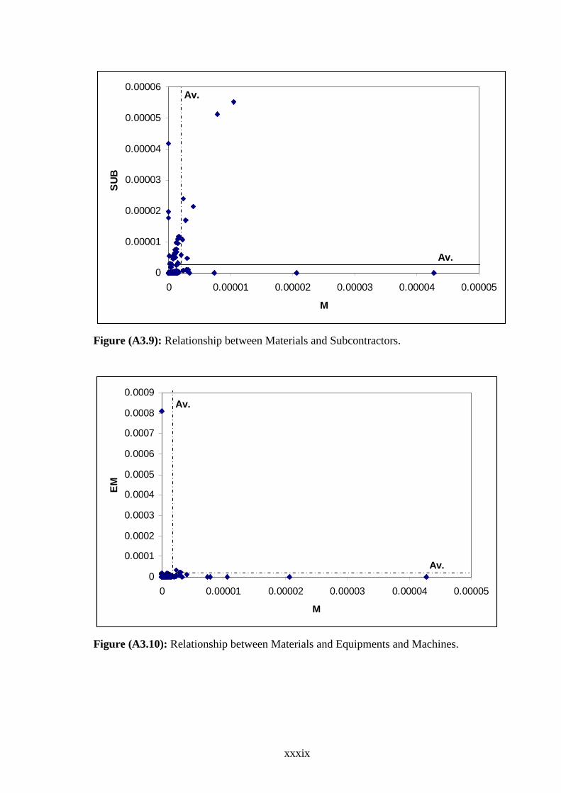
xxxix
0
0.00001
0.00002
0.00003
0.00004
0.00005
0.00006
0 0.00001 0.00002 0.00003 0.00004 0.00005
M
SU
B
Av.
Av.
Figure (A3.9): Relationship between Materials and Subcontractors.
0
0.0001
0.0002
0.0003
0.0004
0.0005
0.0006
0.0007
0.0008
0.0009
0 0.00001 0.00002 0.00003 0.00004 0.00005
M
EM
Av.
Av.
Figure (A3.10): Relationship between Materials and Equipments and Machines.

xl
0
0.05
0.1
0.15
0.2
0.25
0 0.00001 0.00002 0.00003 0.00004 0.00005 0.00006 0.00007
M
MS
Av.
Av.
Figure (A3.11): Relationship between Materials and Management Staff.
0
0.000005
0.00001
0.000015
0.00002
0.000025
0 0.00001 0.00002 0.00003 0.00004 0.00005 0.00006 0.00007
L
CF
Av.
Av.
Figure (A3.12): Relationship between Labor and Cash Flow.
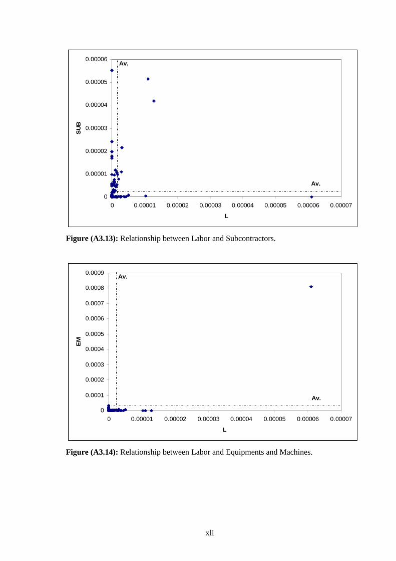
xli
0
0.00001
0.00002
0.00003
0.00004
0.00005
0.00006
0 0.00001 0.00002 0.00003 0.00004 0.00005 0.00006 0.00007
L
SU
B
Av.
Av.
Figure (A3.13): Relationship between Labor and Subcontractors.
0
0.0001
0.0002
0.0003
0.0004
0.0005
0.0006
0.0007
0.0008
0.0009
0 0.00001 0.00002 0.00003 0.00004 0.00005 0.00006 0.00007
L
EM
Av.
Av.
Figure (A3.14): Relationship between Labor and Equipments and Machines.

xlii
0
0.05
0.1
0.15
0.2
0.25
0 0.00001 0.00002 0.00003 0.00004 0.00005 0.00006 0.00007
L
MS
Av.
Av.
Figure (A3.15): Relationship between Labor and Management Staff.
0
0.00001
0.00002
0.00003
0.00004
0.00005
0.00006
0 0.000005 0.00001 0.000015 0.00002 0.000025
CF
SU
B
Av.
Av.
Figure (A3.16): Relationship between Cash Flow and Subcontractors.

xliii
0
0.0001
0.0002
0.0003
0.0004
0.0005
0.0006
0.0007
0.0008
0.0009
0 0.000005 0.00001 0.000015 0.00002 0.000025
CF
EM
Av.
Av.
Figure (A3.17): Relationship between Cash Flow and Equipments and Machines.
0
0.05
0.1
0.15
0.2
0.25
0 0.000005 0.00001 0.000015 0.00002 0.000025
CF
MS
Av.
Av.
Figure (A3.18): Relationship between Cash Flow and Management Staff.

xliv
0
0.0001
0.0002
0.0003
0.0004
0.0005
0.0006
0.0007
0.0008
0.0009
0 0.00001 0.00002 0.00003 0.00004 0.00005 0.00006
SUB
EM
Av.
Av.
Figure (A3.19): Relationship between Equipment and Machines, and Subcontractors.
0
0.05
0.1
0.15
0.2
0.25
0 0.00001 0.00002 0.00003 0.00004 0.00005 0.00006
SUB
MS
Av.
Av.
Figure (A3.20): Relationship between Subcontractors, and Management Staff.

xlv
0
0.05
0.1
0.15
0.2
0.25
0 0.0001 0.0002 0.0003 0.0004 0.0005 0.0006 0.0007 0.0008 0.0009
EM
MS
Av.
Av.
Figure (A3.21): Relationship between Machines, and Management Staff.