Measuring the effects of institutions on economic performancewith the Synthetic Control Method

Luigi MorettiUniversity of Bologna

IOEA 2016, Cargese, May 17, 2016

luigi.moretti7@unibo.it

The problem

� Comparative studies → the evolution of an aggregate outcome for the units affected by theintervention vs the evolution of the same aggregate for the units in the control group.

� The control group might not be a good counterfactual, i.e., it might not represent a goodapproximation of the treated units in the absence of treatment.

– Less formal comparisons: e.g., EU vs US; a EU country vs EU28; a country vs its neighbors;etc.

– Panel data: e.g., Before-and-After or Diff-in-Diff.

→ Common trend assumption needs to be satisfied (testable).

� Sometime we are interested in:

i. Studying only a single treated unit, because:

– it is the only observable event-unit pair;

– different timing of the treatment;

– need of a unit-specific measure of the effect.

ii. Studying the dynamics of effects.

1

The problem

� Comparative studies → the evolution of an aggregate outcome for the units affected by theintervention vs the evolution of the same aggregate for the units in the control group.

� The control group might not be a good counterfactual, i.e., it might not represent a goodapproximation of the treated units in the absence of treatment.

– Less formal comparisons: e.g., EU vs US; a EU country vs EU28; a country vs its neighbors;etc.

– Panel data: e.g., Before-and-After or Diff-in-Diff.

→ Common trend assumption needs to be satisfied (testable).

� Sometime we are interested in:

i. Studying only a single treated unit, because:

– it is the only observable event-unit pair;

– different timing of the treatment;

– need of a unit-specific measure of the effect.

ii. Studying the dynamics of effects.

→ The synthetic control method for comparative case studies developed by Abadie et al. (2003AER, 2010 JASA, 2014 AJPS).

2

This presentation

i. Brief presentation of the SCM.

(a) How does it work?

(b) Advantages and Disadvantages.

ii. Conditions for applying the SCM.

� Brief review of the papers using the SCM.

iii. Focus: Measuring the impact on GDP and productivity of EU membership.

3

Definition

� SCM is a methodology that provides a systematic way to select comparative case studies.

� It compares the evolution of an outcome variable for a treated unit against the evolution of theoutcome for a weighted control group (or synthetic unit).

� Researcher specifies: (1) treatment unit (2) pre-treatment and treatment periods, (3) matchingcovariates/predictors, and (4) donor units (control group).

� The construction of the synthetic unit is made by searching for a weighted combination of thedonor units, so to mimic as close as possible the treated unit’s pre-treatment characteristics.

� Then, the synthetic outcome in the treatment period is given by the weighted combination ofthe donor units’ outcome, using the weights computed in the pre-treatment period. The post-treatment difference between the actual and synthetic outcome is interpreted as the treatmenteffect.

4

Example: Germany’s reunification (Adabie et al. 2015, AJPS)

5

Control units’ weights

Germany’s reunification (Adabie et al. 2015, AJPS)

6

Predictors’ balance

Germany’s reunification (Adabie et al. 2015, AJPS)

7

Example: Campos, Coricelli, Moretti 2014 CEPR dp

Donor W Donor WALB 0 JPN 0.066ARG 0 KOR 0AUS 0 MAR 0BRA 0.142 MEX 0.008CAN 0 MYS 0.001CHL 0.237 NZL 0.116CHN 0 PHL 0.239COL 0 THA 0EGY 0 TUN 0IDN 0 TUR 0ISL 0.19 URY 0

Predictors PRT Synth-PRTReal GDP pc* 9851.037 9839.439

Investment share* 23.669 22.861Pop. growth* .005 .0183

Share of agriculture** 21.999 13.751Share of industry** 30.775 37.725Tertiary education** 10.578 17.556

Secondary education** 49.59153 66.352

Note: sample of control countries from Bover and Turrini (2010).* Source: Penn World Tables.

** source: World Development Indicators.Note: results are robust to different donor samples and model specifications.

8

(A little bit more) technically

� Y is the outcome variable.

� T=T0+T1, where T0 is the pre-treatment and T1 the treatment period.

τj,t = Y Ij,t − Y C

j,t, where Y Cj,t is unknown for t > T0.

� J+1 units; j=1 is the treated, j=2,...,J+1 are potential comparisons (donor pool).

� A synthetic control can be represented by a (Jx1) vector of weights W=(w2,...,wJ+1)’, with0 <= wj <= 1 for j=2,...,J+1 and w2+...+wJ+1=1.

– Let X1 a (kx1) vector of pre-treatment characteristics of the treated unit.

– Let X0 a (kxJ) matrix of the same pre-treatment characteristics of the donor units.

– W ∗ are chosen such that X1-X0W is minimized.

* Given v the relative predictive power of the m-th variable/characteristic,

* W minimizes∑k

m=1 vm(X1m −X0mW )2

� Abadie et al. (AER 2003, JASA 2010) show that τ1,t = Y I1,t −

∑J+1j=2 wjYj,t, for t > T0.

9

Advantages and Disadvantages

The advantages of the SCM:

i. It allows to estimate the effects of single, unit-specific events.

� It allows to estimate the heterogeneous effects of the treatment on each of the treated units.

ii. It allows an assessment of the effects of treatment over time.

iii. It is transparent about the weights assigned to donor units.

iv. When estimations are repeated across units, it allows to construct a unit-time specific measureof the treatment effect, which can be used as dependent variables in a regression to explain theheterogeneity of the effects.

Potential problems related to the SCM:

� Post-treatment shocks on the donor units can bias the results.

– Confidence on the goodness of the synthetic decreases over time.

� It does not allow assessing the significance of the results using standard (large-sample) inferentialtechniques.

– Several attempts to solve these problems: placebo-studies, different donor samples.

10

Conditions for applying the SCM

i. Choice of the relevant outcome variable.

� So far, SCM has been mostly used in macro studies (time-series needed) → the outcomevariable should be likely affected by the treatment.

11

Outcome variable: GDP...

The SCM has been applied to study the effects of several events on GDP, e.g.:

� Terrorism in the Basque Country (Abadie and Gardeazabal 2003 AER)

� Natural disasters (Cavallo et al. 2013 REStat)

– Even extremely large disasters do not display any significant effect on economic growth.

� Germany’s reunification (Abadie et al. 2015 AJPS).

– West Germany GDP fall after reunification.

� Trade liberalizations (Billmeier&Nannicini 2012 REStat).

– Liberalizations had positive effects in most regions, but more recent liberalizations, in the1990s and mainly in Africa, had no significant impact.

� The presence of Mafia activities (Pinotti, EJ 2015).

– Mafia lowered the GDP per capita by 16% in Apulia and Basilicata.

� Civil wars (Dorsett, EJPE 2013; Costalli, Moretti, Pischedda, 2014 wp).

� EU membership (Campos, Coricelli, Moretti, 2014 and 2015 CEPR dp).

� Etc...

12

...but also other aggregate outcomes

Others have looked at different outcomes; eg:

� Effects of political connections on firms’ performance (Acemoglu et al. 2016 JFinEc).

� Effects of anti-tobacco regulation on number of smokers (Abadie et al. 2012 JASA).

� Effects of oil discoveries on democracy (Masi and Ricciuti 2016 UNU-Wider wp).

� Etc...

13

Conditions for applying the SCM

i. Choice of the relevant outcome variable.

� So far, SCM has been mostly used in macro studies (time-series needed) → the outcomevariable should be likely affected by the treatment.

ii. Clear definition of beginning of the treatment.

� Random shocks (easy); Reforms (anticipation effects?); etc.

14

Definition of the treatment unit and treatment period

� E.g.: Pinotti (2015, EJ) on effects of Mafia activities on regional GDP.

15

Conditions for applying the SCM

i. Choice of the relevant outcome variable.

� So far, SCM has been mostly used in macro studies (time-series needed) → the outcomevariable should be likely affected by the treatment.

ii. Clear definition of beginning of the treatment.

� Random shocks (easy); Reforms (anticipation effects?); etc.

iii. Definition of the pre-treatment period.

� It should be long enough when compared to the treatment period.

� Short pre-treatment periods can raise concerns about the goodness of the counterfactualduring the treatment period. We need to show that pre-treatment fluctuations of the treatedunit’s outcome are matched by fluctuations of the synthetic’s outcome (data availabilityconstraints? shocks?).

16

Definition of the pre-treatment period

(Adabie et al. 2015, AJPS)

17

Pre-treatment matching period and Pre-treatment training period

� Pinotti (2015, EJ) divides the pre-treatment in

i. matching period: choice of the weights.

ii. training period: projection during the pre-treatment period → no difference expected.

18

Treatment projection period

� Confidence on the goodness of the counterfactual gradually reduces from the treatment year.

� Data availability constraints.

� Shocks.

19

Conditions for applying the SCM

i. Choice of the relevant outcome variable.

� So far, SCM has been mostly used in macro studies (time-series needed) → the outcomevariable should be likely affected by the treatment.

ii. Clear definition of beginning of the treatment.

� Random shocks (easy); Reforms (anticipation effects?); etc.

iii. Definition of the pre-treatment period

� It should be long enough when compared to the treatment period.

� Short pre-treatment periods can raise concerns about the goodness of the counterfactualduring the treatment period. We need to show that pre-treatment fluctuations of the treatedunit’s outcome are matched by fluctuations of the synthetic’s outcome (data availabilityconstraints? shocks?).

iv. Definition of the preferred/main control sample

� On the base on literature, theory, and goodness of pre-treatment fit.

� Donor units should not be affected by the treatment (spillovers?) and large idiosyncraticshocks during the entire period of analysis (confounding?).

20

Problems with standard inferential techniques

� Post-treatment shocks on the donor units can bias the results.

� This method “does not allow assessing the significance of the results using standard (large-sample) inferential techniques, because the number of observations in the control pool and thenumber of periods covered by the sample are usually quite small in comparative case studies”(Billmeier and Nannicini, REStat 2013).

21

Placebo experiments

� Construct a synthetic counterfactual for each donor unit using the rest of the donor units aspotential controls.

� If the effect on the treated unit is extreme respect to the effects on the donor units (ie. placeboeffects), then we can be confident of the significance of the treatment (eg. Abadie et al., 2010,2014; Billmeier and Nannicini 2012).

22

23

Comparing treated and placebo effects

(Adabie et al. 2015, AJPS)

24

Limits of placebo experiments on donor units

Placebos are informative but

� They do not tell us whether our results are driven by spurious effects.

� They still suffer of small numbers problems.

� For instance (extreme cases):

– Idiosyncratic shocks can affect some countries in the donor sample but these countriesactually take a weight of 0 for the construction of the synthetic country→ the effect on thetreated is not extreme respect to the effect on the untreated (placebo) countries.However, the estimated effect is not spurious.

– The effect on the treated is larger than 95% of the placebo effects and the donor countrieswith larger shocks take a positive weight → the effect on the treated is extreme.However, the estimated effect is spurious.

25

How to complement placebo evidence?

Try different donor samples...

� Each donor sample has its own probability of being affected by (minor or large) shocks on thedonor countries.

� Thus, each set of weight has its own probability to lead to biased results.

� Eg: Billmeier and Nannicini (2012) run to alternative experiments (whole sample and neigh-boring countries).

� Eg: Abadie et al (2010, 2014) exclude one country per time from the donor sample and re-runthe estimation on the treated unit.

26

Leave-one-out

27

EU Membership (Campos et al. 2014, CEPR dp)

� Problem: False perception of abundance of evidence on economic benefits of EU membership.As noted by Eichengreen the main difficulty is to construct relevant counterfactuals; his guessis that EU membership has between +5 and +20% effect on GDP.

� Question: What would have been the growth rates of per capita GDP and labor productivity inEU countries had they not become full-fledged EU members?

� Method : SCM.

� Sample: Non-founding EU countries (17 countries for the 1973, 1980s, 1995, and Eastern EUenlargements).

� Results: In case of non-EU, in these countries GDP per capita would have been, on average,10% lower (but large heterogeneity).

28

29

30

Testing confidence of the results

� Each donor sample has its own probability of being affected by (minor or large) shocks on thedonor countries.

� Thus, each set of weight has its own probability to lead to biased results.

� Eg: Billmeier and Nannicini (2012) run to alternative experiments (whole sample and neigh-boring countries).

� Eg: Abadie et al (2010, 2014) exclude one country per time from the donor sample and re-runthe estimation on the treated unit.

� We suggest a new test and show estimations obtained using randomly chosen (via boot-strapping) donor samples:

– Starting from the whole set of potential comparison countries, we randomly construct 1,000alternative donor samples (each consisting of the same number of countries than our preferreddonor sample). If our main estimation is ’in line’ respect to most of the 1,000 alternativeestimations (with a similar pre-treatment RMSPE), then we can attach a higher level ofconfidence to our results.

31

� SYNTHETIC COUNTERFACTUALS: RANDOM DONOR SAMPLES

– Real GDP per capita

32

33

34

Explaining the gap

It is important to understand the variation across countries and over time in terms of the dividendsfrom EU membership.We show the association between finance and the dividends from EU membership, after controllingfor other factors:

GAPc,t = α + βGAPc,t−1 + θEuroc,t + σFinIntc,t + γTradec,t + εmt. (1)

where:

� GAP is the percentage difference between actual and synthetic GDP series;

� Euro is a dummy variable for countries which joined the common currency;

� FinInt is: (int.liabilities + int.assets)/GDP;

� Trade openess;

� Other controls (e.g. regulation) & country FE & year FE.

35

VARIABLES (1) (2) (3) (4) (5) (6)

Lag percentage gap 0.88652*** 0.87666*** 0.86106*** 0.87993*** 0.84658*** 0.85974***(0.035) (0.034) (0.042) (0.036) (0.046) (0.047)

Trade openness 0.16355*** 0.14280*** 0.15345*** 0.14225*** 0.15448*** 0.13401***(0.031) (0.026) (0.028) (0.027) (0.029) (0.032)

Financial integration -0.00072 0.01238*** 0.01210*** 0.01236*** 0.01246*** 0.01153**(0.002) (0.005) (0.004) (0.005) (0.005) (0.005)

Financial integration (sq) -0.00045*** -0.00037*** -0.00045*** -0.00037*** -0.00036***(0.000) (0.000) (0.000) (0.000) (0.000)

Euro 0.01391* 0.01440* 0.01127 0.01389* 0.01321* 0.02557***(0.008) (0.007) (0.008) (0.008) (0.008) (0.010)

EPL -0.00399 -0.00301 -0.07847***(0.007) (0.007) (0.025)

EPL (sq) 0.01633***(0.005)

ETCR 0.01353** 0.01465** 0.02218*(0.005) (0.006) (0.011)

ETCR (sq) -0.00009(0.002)

Polity2 0.00292 -0.00729 -0.68723*(0.004) (0.007) (0.376)

Polity2 (sq) 0.03728*(0.021)

Political constraints 0.00728 -0.00715 -0.06330(0.027) (0.034) (0.256)

Political constraints (sq.) 0.04525(0.321)

Year of membership 0.00222*** 0.00286*** 0.00368*** 0.00284*** 0.00398*** 0.00256**(0.001) (0.001) (0.001) (0.001) (0.001) (0.001)

Country & Year dummies Yes Yes Yes Yes Yes Yes36

Campos, Coricelli, Moretti 2015 (CEPR dp)

� Extension: Can we disentangle the effects of deep (i.e. political plus economic) integrationfrom those of shallow (i.e. economic only) integration?

� One natural experiment: Norway 1995.

� We find that productivity of Norwegian regions would have been on average 6% higher between1995 and 2000 if Norway had taken full EU membership.

37

Research design

� Our identification strategy uses the 1995 EU Northern Enlargement:

– In January 1994, four countries (Austria, Finland, Norway, and Sweden) joined the EEA (i.e.,enjoyed the benefits from economic integration with the EU through the Single Market).

– They were all ready to gain full EU-membership from January 1995 (enjoying the benefitsfrom economic plus political integration).

– In November 1994, in a referendum, 52.2% of Norwegians voted against the EU membership.

– Since January 1995, AT, FI, and SE are full EU members, while Norway is only EEA member.

� We employ two different estimation approaches:

– Difference-in-differences.

– Synthetic control method (SCM).

38

Data

� Period of analysis is 1988-2000: 1988-1994 (pre-treatment); 1995-2000 (post-treatment).

– After 2000: (i) AT and FI adopted Euro; (ii) EU forced Norway to adopt more commonregulation and eliminate its system of special taxation of remote areas; (iii) Norway increasedgas exports.

� Data (NUTS2) from Cambridge Econometrics European Regions Dataset (see Becker et al.JPubE 2010, and Tabellini JEEA 2010).

– We focus on productivity (results are robust to the exclusion of Energy sector).

39

BEFORE AND AFTER 1995: Average difference by region

40

Example

Donor W Donor WBurgenland (AT) 0.19 Lansi-Suomi (FI) 0.00

Niederosterreich (AT) 0.00 Pohjois-Suomi (FI) 0.00Wien (AT) 0.00 Aland (FI) 0.09

Karnten (AT) 0.00 Stockholm (SE) 0.00

Steiermark (AT) 0.00 Ostra Mellansverige (SE) 0.00Oberosterreich (AT) 0.00 Smaland med arna (SE) 0.11

Salzburg (AT) 0.00 Sydsverige (SE) 0.00Tirol (AT) 0.61 Vastsverige (SE) 0.00

Vorarlberg (AT) 0.00 Norra Mellansverige (SE) 0.00Ita-Suomi (FI) 0.00 Mellersta Norrland (SE) 0.00

Etela-Suomi (FI) 0.00 Ovre Norrland (SE) 0.00

Predictors Actual SynthLags prod.* 19.65 19.67

Investment sh.* 0.24 0.27Pop. Density* 0.02 0.05

Sh. Agric.* 0.04 0.14Sh. Man.+Energy* 0.22 0.18

Sh. Services* 0.35 0.36Sec. Education** 8.65 10.24

* Source: Cambridge Econometrics.** source: Gennaioli et al. (2014)

Note: results are robust to different donor samples and model specifications.

41

42

THE SYNTHETIC CONTROL METHOD: Average effects by region

43

Placebo experiment on each treated unit

� Abadie et al (2010) suggest to run fake experiments on the control units and assess whetherthe effect on the treated unit is extreme respect to the effect of the placebo treatment on thecontrols.

44

45

Placebo experiments on treated group

� We follow Acemouglu et al. (forthcoming, JFinEc) and construct placebo groups (of the samedimension of the treated group), so to compare whether the average treatment effect on thetreated group is extreme respect to the effects on the placebo groups.

i. We construct 1,000 placebo groups of seven regions randomly chosen from the group ofdonor regions.

ii. We estimate a synthetic counterfactual for each region in each group.

iii. We compute an average effect in each group (weighted by the regions’ goodness of pre-treatment fit).

iv. We compare the average effect on the treated group of Norwegian regions with the effectsfound for the 1,000 placebo groups.

46

Placebo experiments on treated group

� The effect on the treated group of Norwegian regions (black vertical line) is at the left of the2.5th percentile of the distribution of placebo effects (red line) → it is negative and extremerespect to placebo effects.

47

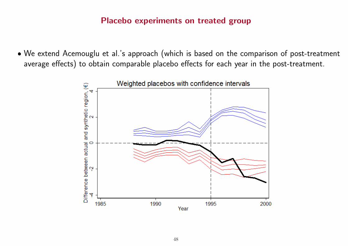
Placebo experiments on treated group

� We extend Acemouglu et al.’s approach (which is based on the comparison of post-treatmentaverage effects) to obtain comparable placebo effects for each year in the post-treatment.

48

Random donor samples

49

50

Interpreting the results

� After 1995, in any Norwegian region (except for Oslo) productivity is lower respect to itscounterfactual.

� Explaining heterogenous effects:

– Peripheral regions represent traditional sectors.

– Norway’s regional policy aimed at protecting and subsidizing those activities.

– Negative effects on relative productivity.

– Oslo, with high level of human capital, and efficient public and financial sectors: able toexploit higher benefits of economic integration without political integration.

– In summary: lacking political integration allowed rent seeking behavior of peripheral regions(Brou and Ruta’s argument).

� Voting in EU referendum can help us to interpret the results:

– Peripheral regions (protected from national policies) voted for staying out of the EU; Oslovoted for joining the EU.

51

Conclusion

� SCM allows to run causal inference analysis IN THE FRAMEWORK OF COMPARATIVE CASESTUDIES.

� SCM allows to obtain a unit-specific time-varying estimate of the treatment effects.

� A growing number of papers using this method.

� Appealing for media reports (intuitive method + a single number/effect for each treated unit).

� Need of developing the method to propose systematic ways to assess the statistical significanceof the estimates.

52