Measuring the distance of vegetation from powerlines …vision-cdc.csiro.au/changs/doc/sun-etal06ijprs.pdf · Measuring the distance of vegetation from ... of the distance of vegetation

emote Sensing 60 (2006) 269–283www.elsevier.com/locate/isprsjprs

ISPRS Journal of Photogrammetry & R

Measuring the distance of vegetation from powerlines usingstereo vision

Changming Sun a,⁎, Ronald Jones a,1, Hugues Talbot a,2, Xiaoliang Wu b,Kevin Cheong a,3, Richard Beare a,4, Michael Buckley a, Mark Berman a

a CSIRO Mathematical and Information Sciences, Locked Bag 17, North Ryde, NSW 1670, Australiab CSIRO Mathematical and Information Sciences, Private Bag No 5, Wembley WA 6913, Australia

Received 10 September 2005; received in revised form 17 March 2006; accepted 17 March 2006Available online 11 May 2006

Abstract

Electricity distribution companies in many countries are required to maintain a regulated clearance space around all powerlinesfor bushfire mitigation and safety purposes. Vegetation encroachment of high voltage electricity line clearance space is a majorproblem for electricity distribution utilities. If not properly controlled, vegetation encroachment can lead to bushfire and publicsafety risks as well as degrading electricity supply reliability. In this paper we describe a prototype airborne system for theautomated measurement of the distance of vegetation from powerlines using stereo vision from a stream of stereo images. Afundamental problem with the images from the prototype system is that the powerlines are usually difficult to see, although thepower poles are visible. The proposed strategy has been to recover the vegetation surface using stereo vision techniques, identifysuccessive power poles, model the powerlines between successive poles as a catenary, and measure the distance between thevegetation surface and the modelled line. Some suggestions about how to improve the system are also made.© 2006 International Society for Photogrammetry and Remote Sensing, Inc. (ISPRS). Published by Elsevier B.V. All rightsreserved.

Keywords: stereo matching; powerline inspection; power pole segmentation; vegetation clearance; 3D vegetation surface

1. Introduction

Infrastructure components such as powerlines, tele-communication lines, and oil and gas pipelines, are

⁎ Corresponding author. Fax: +61 2 9325 3200.E-mail address: [email protected] (C. Sun).

1 Present address: DSTO Information Sciences Laboratory, Edin-burgh SA 5111, Australia.2 Present address: Laboratoire Algorithmique et Architecture des

Systèmes Informatiques, ESIEE, Paris, France.3 Present address: Bureau of Meteorology, Melbourne Vic 3001,

Australia.4 Present address: Medicine, Nursing and Health Sciences, Monash

University, Vic 3800 Australia.

0924-2716/$ - see front matter © 2006 International Society for PhotogramAll rights reserved.doi:10.1016/j.isprsjprs.2006.03.004

often run above ground, for very long distances,extending in “corridors”. Encroachment of vegetationon the infrastructure components (whether they bepowerlines, telecommunication lines or pipelines) isundesirable. Vegetation may damage powerlines ortelecommunication lines, or limit access to pipelines.However one of the most disastrous outcomes isbushfire, resulting from contact between powerlinesand vegetation. Inspection of infrastructure corridors istherefore required to monitor vegetation.

Current methods for checking clearances involvelaborious, ground or airborne based visual inspection ofelectricity distribution networks to determine whichtrees must be cleared, together with extensive aerial

metry and Remote Sensing, Inc. (ISPRS). Published by Elsevier B.V.

mailto:[email protected]

http://dx.doi.org/10.1016/j.isprsjprs.2006.03.004

270 C. Sun et al. / ISPRS Journal of Photogrammetry & Remote Sensing 60 (2006) 269–283

audits of the network to ensure effective clearance priorto the bushfire season. These are expensive, timeconsuming, sometimes dangerous, and subject toobserver bias and fatigue or a failure to observe troublespots at the right time. Further, human beings are notvery good at judging perspective from a distance. It maytherefore be difficult to tell from a supervised inspectionwhether vegetation is encroaching on infrastructurecomponents or not. For example, when a powerline isbeing inspected from an aircraft, the inspector is usuallyrequired to observe the line from directly above. In thissituation, it is very difficult to judge the distancebetween the vegetation and the lines.

There is a need for a system and method whichenables the automated mapping or inspection ofcorridor-type infrastructure. Such a system shouldquantify encroachment by vegetation and detect otherfaults, thus enabling correct maintenance planning. Anumerical method for predicting the performance of apowerline proximity warning device installed on avehicle equipped with any type of boom has beenproposed (Nguyen et al., 1996). Remote sensingtechniques have been used for land-cover anomalydetection along pipeline rights-of-way and for trans-mission corridor encroachment detection (Gauthier etal., 2001; Campanella et al., 1995). The imageresolution for currently available remotely sensedimages is still low. A photogrammetric solution, calledDanger Tree, has been developed using aerial photog-raphy (Dall, 1991). It requires a number of parametersabout the transmission lines. It also requires aerialphotographs on two occasions: once when the treeshave no leaves, and once when the tree leaves are attheir fullest. Jones and colleagues have developedtechniques for aerial inspection of overhead powerlinesusing video on a helicopter platform (Jones, 2000;Jones and Earp, 2002; Whitworth et al., 2001; Williamset al., 2001; Jones et al., 2003; Golightly and Jones,2003, 2005). However, they have not been used formeasuring the distance between powerlines and nearbyvegetation. Laser range finding techniques havesometimes been used for such purposes (Ackermann,1999; Carter and Shrestha, 1998; Hyde et al., 1996;FLI-MAP, 2005). Systems which use laser scanningtechniques tend to be more expensive than systemsusing video cameras. Even with laser range findingtechniques, video images are often needed for visualinterpretation purposes. In this project, we study thepossibility of developing a cost effective airborneimage capture and processing system to automaticallymeasure the clearance of vegetation from powerlines tosupport bushfire mitigation operations.

The paper is organised as follows. Section 2 givesa brief description of the prototype system and ourapproach. Section 3 describes our methods for stereoimage processing, including camera orientation esti-mation and stereo image normalisation, dense stereomatching, and 3D calculation. We present ourmethods for power pole segmentation using thenormalised stereo images in Section 4. The digitalelevation model (DEM) and orthoimage generationand mosaicking are presented in Section 5. Thedistance calculation, computational speed and accura-cy, and visualisation aspects are presented in Sections6, 7 and 8 respectively. Finally in Section 9 we makesome suggestions about how the system might beimproved.

2. The prototype system and our approach

In this prototype system, a fixed-wing aircraft(Cessna 182RG) flies at approximately 80 m abovethe ground, with forward looking video cameras thatcapture a continuous series of color images of thepowerline infrastructure mounted beneath the tip ofeach wing. (The flying height for a fixed-wing aircraftis of necessity much higher than that for a helicopter,which is usually between 3 and 10 m above thepowerlines.) The angle between the optical axes of thetwo cameras is about 7°. The cameras are lookingdown at about 35° (i.e. the angle between the opticalaxis and the horizon is about 35°). The pixel resolutionon the ground is about 10 cm close to the centre of theimage. The distance between the two cameras is 10 m.The system carries a differential global positioningsystem (DGPS) and an inertial navigation system(INS) to provide position and orientation data for theaircraft. The accuracy of the DGPS is better than0.5 m. Fig. 1 gives a schematic illustration of thesystem.

A fundamental problem with the images currentlyavailable is that the powerlines are usually difficult tosee, although power poles are visible. The proposedstrategy is to identify successive power poles, and tomodel the lines between poles as a catenary. In fact,because of variations in line tension with load,temperature, etc., a range of catenary curves will beused, resulting in a catenary “envelope”. The aim is thento measure the distance from the envelope to nearbyvegetation. Another complication is that successivepower poles are in different image “frames”, usuallyabout 10 to 14 images apart. Frames between successivepower poles need to be “mosaicked” into a single pole-to-pole image in order to measure the distance between

Fig. 1. A fixed-wing aircraft flying above powerlines and collecting streams of stereo images.

271C. Sun et al. / ISPRS Journal of Photogrammetry & Remote Sensing 60 (2006) 269–283

the catenary envelope and the trees. Therefore thestrategy used in this project is:

(1) Use stereo vision to obtain a 3D surface fromvideo images.

(2) Find the power poles automatically from imagesand match them in stereo images.

(3) Mosaic the images to create a pole-to-pole image.(4) Infer the catenary envelope in each pole-to-pole

image.(5) Calculate the distances from the catenary enve-

lope to trees.

The following steps will need to be carried out toproduce the relevant information in a pole-to-poleimage and they are described in detail later in thispaper:

(1) Automatically calculate the relative orientation ofthe stereo cameras for each pair of images, sincewind and vibration effects continually change thecamera geometry.

(2) Normalise individual image pairs to generateepipolar stereo images based on the relativecamera orientation.

(3) Match individual image pairs to obtain disparitymaps.

(4) Identify power poles using image information.(5) Compute 3D information from matched pairs.

This step includes the calculation of the 3Dpositions of the tops of the power poles and the 3Dsurface of each 3D scene.

(6) Calculate the catenary envelope of powerlinesusing the 3D positions of the tops of the poleswithin a span.

(7) Generate a DEM using the disparity map andcamera parameters; generate an orthoimage usingthe DEM, image and camera information.

(8) Mosaic the DEM and orthoimages into a 3D pole-to-pole image.

(9) Identify tree boundaries in each 3D pole-to-poleimage.

(10) Measure appropriate distances from the catenaryenvelope to tree boundaries.

3. 3D reconstruction using stereo vision

3.1. Input camera parameters and stereo images

There are 6 external parameters recorded thatdescribe the position and orientation of each camerawhen each image was acquired. These are related to theDGPS and INS measurements. The internal cameraparameters are also known through camera calibration.These parameters, identical for each image, are: camerafocal length, camera lens distortion, pixel size of theCCD array in the X direction, pixel size of the CCDarray in the Y direction, and the location of the principalpoint. Both the internal and the external parameters willbe used in 3D calculations. The color images wereinitially recorded on SuperVHS tapes, and digitised off-line. These VHS tapes have been used before this studyfor visual checking of the power poles. The image size is736×560 pixels. In future systems, digital cameras willbe used for image acquisition. For each pole-to-polespan, there are usually 10 to 14 frames. They are obliqueviews of the scenes. In this project, only lightnessinformation has been used to match image points. Thelightness image is obtained by averaging the red, greenand blue bands of the original color image. Color

Fig. 2. (a,b) One pair of the normalised stereo images; (c) the disparityimage obtained (notice the shadow region of the tree on the ground hasthe same disparity as the rest of the ground).


information was used in the power pole segmentationstage.

3.2. Camera orientation and image normalisation

The relative camera parameters do not stay constantdue to vibration of the aircraft wings, so it is necessaryto estimate the true camera orientation parametersautomatically from image features. We used Zhang etal.'s method for robust feature matching (Zhang et al.,1995). Because the point matching step is automatic,mismatches can occur. Therefore it is necessary toidentify and remove those mismatches for theestimation of the camera geometries. The parametersrelated to this geometry include the three rotationangles and the three elements of the translation vector(two elements if normalised). The geometry obtainedwill be used for stereo image normalisation and for 3Dcalculation.

After the relative orientation parameters of thecameras have been obtained, stereo image normalisationcan be performed. The operation of normalisation ismeant to ensure a simple epipolar geometry for a stereopair (Faugeras, 1993, Section 6.3). By simple geometrywe mean that the epipolar lines are parallel to the imagerows, i.e. the normalisation process transforms (usuallynon-horizontal) epipolar lines into horizontal scanlines.The new image plane is chosen so that it is parallel to theline connecting the two camera centres (Ayache andHansen, 1988; Ayache and Lustman, 1991; Kang et al.,1994). Normalisation using three images (a stereo pairplus one image in a neighboring pair) can also be carriedout (Sun, 2003). In the normalised stereo images,corresponding points or matching points lie on the samehorizontal scanlines in the left and right epipolar images.This allows for simpler and more efficient dense stereomatching. Stereo image normalisation will also beuseful for power pole segmentation and matching.

3.3. Dense stereo matching

Disparity is the difference in pixel location betweenmatched features in different images. This disparityimage together with the camera parameters can be usedto calculate the 3D surface. We use the normalised leftand right images to generate a disparity map using fastdense stereo matching.

We have developed a fast and reliable stereomatching algorithm which produces a dense disparitymap by using fast cross correlation, rectangularsubregioning (RSR) and 3D maximum-surface techni-ques in a coarse-to-fine (pyramid) scheme (Sun, 1997,

2002). Fast correlation is achieved by using the box-filtering technique whose speed is independent of thesize of the correlation window and by segmenting thestereo images into rectangular subimages at differentlevels of the pyramid. By working with rectangularsubimages, not only can the speed of the correlation befurther increased, the intermediate memory storagerequirement can also be reduced. The disparity mapfor the stereo images is found in the 3D correlationcoefficient volume by obtaining the global 3D maxi-mum-surface rather than simply choosing the positionthat gives the local maximum correlation coefficient


value for each pixel. The 3D maximum-surface isobtained using a two-stage dynamic programming(TSDP) technique. Detailed descriptions of the algo-rithms are given in Sun (1997, 2002). Fig. 2 shows anormalised image and the disparity image obtained byapplying our stereo matching technique.

3.4. 3D calculation

After obtaining the corresponding points (as in adisparity map) between the left and right 2D images, the3D position of the same physical point can be obtained.The coordinates of the 3D point can be obtained byfinding the intersection of the two light rays passingthrough the camera centres and the two image matchingpoints. If we calculate the 3D position for every matchedpoint on the image, a 3D surface of the scene can beobtained. The 3D positions of the tops of the power polesare calculated in the same way. The image positions ofthe power poles are obtained using the method describedin Section 4. The final 3D information is calculated in theglobal reference system, and therefore can be related toother geographical data such as that found in ageographical information system (GIS).

4. Power pole segmentation

The aim of the power pole segmentation procedure isto find the pole when it appears in an image pair andthen to find the position along the pole where thepowerline is attached. Note that there is insufficientresolution in the current set of images to locate the poleinsulators (which would indicate exactly where the lineis attached to the pole). The width of a pole at the top isabout 30 cm. Instead, our approach is to find either theintersection point of the cross arm with the pole or, incases where there is no cross arm attached to the pole, tofind an accurate measure of the top of the pole. Input tothe segmentation procedure is a pair of left and rightnormalised color input stereo images as described in theprevious section.

4.1. Finding candidates for poles and cross arms

The procedure for segmenting candidates for polesand cross arms begins with a preprocessing step to mark‘background’ parts of the image that we know cannotpossibly be poles, in particular green vegetation regions.There are two assumptions made about poles during thisprocessing stage: poles are gray (not green or some othercolor) and poles are light (they are not black and there isadequate lighting on the pole). These two assumptions

are the basis for a simple segmentation procedure to findbackground regions in the image. After transforming thecolor input image into an hue, lightness and saturationimage, the saturation component of this image is thenused to identify regions that are not gray and thelightness component is used to find dark regions.

The next step in the segmentation process is toidentify candidates for poles in the input image (asillustrated by a subimage in Fig. 3a). The sequence ofsteps is as follows:

(1) Perform a linear vertical median filter on thelightness component of the hue, lightness andsaturation image (Fig. 3b).

(2) Perform a horizontal linear median filter on thevertical median filter result and take the absolutedifference between the two images.

(3) Threshold this result and remove those pixelspreviously identified as background pixels(Fig. 3c).

(4) Perform a vertical linear median filter on thisresult to connect up broken line elements andremove isolated noise.

(5) Perform a dynamic line opening (see below for adescription of this new filter) to remove spuriousfeatures on the sides of linear objects.

(6) Remove short lines to produce the final image ofpole candidates (Fig. 3d).

As mentioned above, a new filter called the dynamicline opening is used to clean up linear features in binaryimages. The filter treats each object in the binary imageindependently. The direction θi of the major axis of thebest fit ellipse (Haralick and Shapiro, 1992, Sect. A.7) tothe binary object i is calculated and the maximum lengthLi of the object in direction θi is determined (using aminimum bounding box in direction θi). Then eachobject is filtered by removing line segments (in directionθi) within the object that are shorter than some fractionof Li; in our procedure, this fraction is one half. The filtertends to remove noise from the side of the object andpreserve only the main form of the object.

The process for finding cross arms follows that forfinding pole candidates. As the aircraft is flying alongthe powerlines, the cross arms usually appear approx-imately horizontally in the image. Therefore, thedirection of filters used for cross arm detection arealong the horizontal direction. The number of crossarms on a pole varies. It can be 1, 2, 3 or no cross arms.When there is more than one cross arm, the separationbetween them varies from about 90 to about 210 cmdepending on the type of pole. An example result for

Fig. 3. Finding candidates for poles in the input image. (a) Subset of an input image. (b) Result from the vertical median filter when applied to thelightness component image. (c) Threshold of the absolute difference image between (b) and the result of a horizontal median filter, restricted toregions that are not in the background of the image. (d) Final result after a dynamic line opening and length threshold is applied.


this process is shown in Fig. 4. A few steps for the poleor cross arm detection involve the use of medianfiltering along linear windows. Other methods such asthe Sobel filter or the Hough Transform could also beused for pole or cross arm detection. However, we havefound the above procedure to be satisfactory for ourpurposes.

4.2. Matching candidates for poles and cross arms

After running the background detection, and the poleand cross arm segmentation procedures on both the leftand right normalised images, we have images of poleand cross arm candidates for the image pair. Fig. 5shows an example set of results. The input left and rightimages are shown in Fig. 5a and b respectively. Thecorresponding pole candidates found are shown in Fig.

5c and d and the cross arm candidates found are shownin Fig. 5e and f.

4.2.1. Matching pole candidatesThe first step in the pole matching process is to label

and obtain summary shape statistics (such as area,bounding box and best fit ellipse statistics) for the polecandidates in the left and right images. Any candidatesthat have a small vertical height or are not lying withinthe central region of the image are discarded. We saythat a left and a right candidate form a valid pair of polesif they satisfy the following constraints:

(1) There is vertical overlap of the two candidates.(2) The angular separation between the candidates is

within a specified angle range. Note that a pair ofpole candidates will typically form a ‘V’ shape,

Fig. 4. Finding candidates for cross arms in the input image (as in Fig.3a). (a) Result from the horizontal median filter when applied to thelightness component image. (b) Final result after cleaning andapplying an opening by union.


where the right pole candidate is actuallypositioned to the left hand side of the left polecandidate.

(3) The horizontal distance between the centroid ofthe right and the left pole candidates is within aspecified range.

4.2.2. Matching cross arm candidatesOnce a set of valid pairs of poles has been found, the

next stage in the matching process is to find and matchany cross arms that intersect the pole candidates. Theprocess comprises the following steps for each valid pairof poles:

(1) Fit a line to the left pole candidate in the valid pairthat passes through its centroid at an angle given

by the direction of the major axis of the best fitellipse to the pole candidate.

(2) Find all the cross arm candidates in the left imagethat intersect this line, between two verticalextremes given by the bottom of the polecandidate and the top of the pole candidate plusa few extra pixels.

(3) Record the vertical position of each intersectingcross arm at the centroid point where it intersectsthe line.

(4) Repeat the above process for the pole candidatesin the right image to find the right intersectingcross arms.

(5) Match a pair of left and right intersecting crossarms by finding the pair that has the minimumvertical separation.

(6) Repeat the above step, excluding cross arms thathave already been matched, until either there areno remaining left cross arms or no remaining rightcross arms.

The matching cross arms for the example valid pairin Fig. 5 are shown in Fig. 6. Here, the verticalseparation marks where to search for intersecting crossarms along the line fitted to the pole candidate; in thiscase there are two intersecting cross arms for both theleft and right candidates.

4.2.3. Choosing the best valid pair of pole candidatesWe now have matched valid pairs of pole

candidates and have found any matching crossarms for each valid pair. The final stage in theprocess is to select the best valid pair of polecandidates, which will hopefully correspond to thetrue power pole in the input images. If we considertwo valid pairs of poles A and B, we consider that Ais a better solution than B if it satisfies one of thefollowing conditions:

(1) A has the same number of cross arms as B and hasa greater vertical height than B.

(2) A has more cross arms than B and has at least halfthe vertical height of B.

(3) A has fewer cross arms than B and has at leasttwice the vertical height of B.

By comparing all the valid pairs, the best solution fora valid pair is determined. Fig. 7 shows a collection ofresults superimposed upon the original normalised inputimages. Segmented poles are indicated in black andcross bar intersection points are indicated by whitediscs.

Fig. 5. Results for the pole and cross arm segmentation procedures. (a) Left normalised input image. (b) Right normalised input image. (c) Polecandidates in the left image. (d) Pole candidates in the right image. (e) Cross arm candidates in the left image. (f) Cross arm candidates in the rightimage.


4.3. Poles with no cross arms

In cases where there is no cross arm attached to thepower pole, we need to use the position of the top of thepole as a measure for where the powerline is attached.Therefore, we refine the result given by the polesegmentation procedure using a watershed function(Vincent and Soille, 1991). The watershed functionrequires as input a marker for the pole, a marker for thebackground (called the external marker), and also asegmentation function. The first stage in the process is to

clean and refine the previous segmentation result for thepole so as to obtain a good pole marker. This is done bythe use of the skeleton operation (Serra, 1982) and therank-max opening operation.

We now turn our attention to finding an externalmarker for the watershed function. A rank-min closingis used to fill in regions in the external marker that arenot linear features such as poles. We also make use ofthe pole marker found in the previous section to makesure that the external marker does not overlap the pole.These markers are shown in Fig. 8a, where the pole

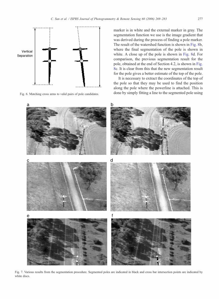
Fig. 7. Various results from the segmentation procedure. Segmented poles awhite discs.

Fig. 6. Matching cross arms to valid pairs of pole candidates.


marker is in white and the external marker in gray. Thesegmentation function we use is the image gradient thatwas derived during the process of finding a pole marker.The result of the watershed function is shown in Fig. 8b,where the final segmentation of the pole is shown inwhite. A close up of the pole is shown in Fig. 8d. Forcomparison, the previous segmentation result for thepole, obtained at the end of Section 4.2, is shown in Fig.8c. It is clear from this that the new segmentation resultfor the pole gives a better estimate of the top of the pole.

It is necessary to extract the coordinates of the top ofthe pole so that they may be used to find the positionalong the pole where the powerline is attached. This isdone by simply fitting a line to the segmented pole using

re indicated in black and cross bar intersection points are indicated by


the best-fit ellipse statistics of centroid and orientation.By inserting the top vertical position into the equationfor this line, the corresponding top horizontal position isreadily extracted.

4.4. Summary results for pole segmentation

We now present a summary of the segmentationresults for several representative spans of images thatwere normalised. Usually a span of images contains 10to 14 image pairs that runs from one pole to the next. Apole will often appear in about four or five of theseimage pairs. Our algorithm will usually find the pole intwo or three of these pairs.

Fig. 8. Applying the watershed function. (a) Combined pole in white and extefinal result for the pole is in white. (c) Original pole candidate superimposed oprocess; the top of the segmented pole is now correctly positioned.

We present results for a set of eight spans. Table 1shows the results for these spans, each of which isindicated by a number 1 to 8 at the top of the table.Under each number is a column of results which givesthe success rate for the span on an image basis and thenan overall success (tick) or fail (cross) classification forthe span. For example, for the first span, 5 out of 5 of theimage pairs that contained a pole were successfullysegmented. By ‘successfully segmented’ we mean thatthe pole was found and the position along the polewhere the powerline is attached was correctly deter-mined (either the pole/cross arm intersection point or thetop of the pole for those poles without cross arms). Forthis same span, 9 out of 9 of the image pairs that did not

rnal markers in gray. (b) Result from the watershed function, where then the image. (d) The improved segmentation result using the watershed

Table 1Summary of results for 8 spans of images

Span 1 2 3 4 5 6 7 8

Success: pole 5/5 5/5 2/4 4/4 3/6 1/3 6/6 4/4 30/37 (81%)Non pole 9/9 8/8 8/8 9/9 4/5 11/11 6/6 17/17 72/73 (98%)Failure: pole 2/4⁎ 3/6⁎ 2/3⁎ 7/37 (19%)Non pole 1/5 1/73 (2%)Success √ √ √ √ × × √ √

Success (tick) or fail (cross). Asterisk denotes failures due to poor image quality. See Section 4.4 for details.


contain poles were correctly segmented. That is, theprocedure returned no pole objects for these images andwas not fooled into finding an object that was not a pole(for example a branch of a tree or a fence post). Overallthen, we have determined that this span was a successand this is indicated by the tick at the bottom of thecolumn.

As any given pole will appear in two or threeconsecutive images, we only need to segment the poleand correctly determine the position of the powerline inany one of these images. Therefore, it is possible for thesegmentation procedure to fail to find a pole in a singleimage pair but find it in another image pair; this will berecorded as an overall success for the span. We denotefailures due to poor image quality in Table 1 with anasterisk (in fact, most of the failures were caused bypoor image quality, as discussed further below).

Span 5 in Table 1 shows the only case where therewas a failure on an image pair that did not contain a pole.Overall, 6 out of the 8 spans processed were deemed tobe successfully segmented. On an image basis, 81% ofthe image pairs that contained poles were successfullysegmented (as indicated on the right hand side of thetable) and 98% of the image pairs that did not containpoles were successfully segmented.

5. DEM and orthoimage generation and mosaicking

5.1. DEM and orthoimage generation

Since the powerlines cannot be seen in the majority ofthe images, their position will be modelled using theknowledge of where the power poles are. This requiresconsecutive power poles to appear in a single image.Unfortunately, power poles are several images apart. Inthe first sequence of test images, power poles appear inapproximately every 10th to 14th image in the sequence.In some of the more recent test images, particularly theset over a typical rural network, power poles are moreunevenly spaced. To create the pole-to-pole images, weneed to generate a DEM and orthoimages. In our case theknown output image grid will be the Australian Map

Grid. The location of each data item is given in eastingand northing coordinates which have been interpolatedonto a regular grid. This means that information derivedfrom these images can easily be related to othergeographical data.

From the 3D calculation stage, each pair of matchingpoints generates a point in 3D space. Within the field ofview of the cameras, all the 3D points which havecorresponding image matching points have a 3Dlocation measurement. However, the 3D points obtaineddo not lie on a regular grid. From these irregular 3Dpoints, interpolation was performed in the local regionto obtain the 3D points on a regular grid (Bartier andKeller, 1996). The grid spacings or the distances ofneighboring points in the X and Y directions need to begiven. The spacing of the grid will relate to the size ofthe DEM.

After the DEM of a local region has been obtained, itscorresponding orthorectified image or orthoimage can begenerated. Generating an orthoimage needs the DEM,camera parameters (internal and external) and theoriginal image. For each element in the DEM, weknow its 3D X, Y, and Z position. Using the knowncamera parameters, its corresponding image location of aDEM position can be obtained using the collinearityequations (Kraus, 1993, p.278). Therefore we have acorresponding image intensity value related to this DEMposition. This obtained image location is unlikely to be atthe exact position of a pixel in the input image grid. Theimage intensity value in the output image is determinedby bilinear interpolation. Fig. 9a shows an image of theDEM obtained from Fig. 2a and b. The black coloraround the borders of the image indicates missing values.The pixel intensity in Fig. 9a relates to the heights ofDEM. Fig. 9b shows the obtained orthoimage.

5.2. Mosaicking of DEMs and orthoimages

Once the images have been aligned on a commongrid, mosaicking is performed to overlay the images oneach other. In the regions where the images overlap, adecision needs to be made about how to determine what


intensity values are transferred to the output image. Theoptions are to place one image on top of (overwrite) theother or to average the intensity values of the two (ormore) images. The latter option can produce a visuallysmoother image by smoothing any overall brightnessdifferences between the images, but if the alignment ofthe images is not sufficiently accurate, it can also causespatial blurring of image features in the overlap region.The overwriting option will be used for these examples,since the time lapse between successive images isminimal, and hence illumination differences should beminimal.

Fig. 9. (a) DEM. The black color around the borders of the imageindicates missing values. The pixel intensity relates to the heights ofDEM. (b) Orthoimage corresponding to (a).

Fig. 10. (a) Mosaicked DEM and the (b) mosaicked orthoimages.

It is also necessary to mosaic several orthoimagesinto a single large orthoimage. Both DEM and ortho-image information are necessary to mosaic orthoimagesgeometrically, since the geometric information isprovided by the DEM. Fig. 10 shows the mosaickedDEM (from 14 DEMs) and the corresponding mosa-icked orthoimage. Due to small errors on the externalorientation parameters, the joining for several smallblocks of DEMs at the bottom of the mosaicked DEM inFig. 10 seems unsmooth. This effect can be reduced if abundle adjustment process is carried out for estimatingthe external orientation parameters within a span so thatthe parameters from neighboring pairs are consistentwith each other.

6. Measuring the distance of trees from powerlines

This section explains how the distance from thepowerline to neighboring trees and vegetation is

Fig. 11. (a) Top view of a powerline (with envelope) suspended on 2power poles over a landscape. (b) Side view of a powerline and allobjects in the landscape. (c) Side view of a powerline and objectswithin the catenary envelope (powerline sagging in (b) and (c) hasbeen magnified). Powerline represented as white pixels. The gray levelintensities are proportional to the height of each pixel in the landscape.The catenary envelope is represented by black pixels, and vegetationfound within the catenary envelope is represented by white blobs.


calculated. It then describes a method of determining ifthe vegetation lies within an envelope centred about thepowerline. The calculation of distances from thepowerline to the underlying surface is performed afterthe full 3D surface between two power poles has beengenerated, using stereo matching and mosaicking. Thismethod is illustrated using a span of mosaicked imagesof landscapes which contains a powerline suspendedbetween two power poles.

The input data is a landscape (3D surface) stored inDEM data format. A pixel in the image has a gray levelintensity which corresponds to the height of thelandscape at that pixel point. Now, given the 3Dlocation of the tops of two power poles, we can calculatethe location of the powerlines modelled by a catenary,the envelope that surrounds the powerlines and decidewhether vegetation lies within this envelope.

The minimum safe distance of an object to thepowerline is known as a clearance. This measure isgiven for a specific conductor type and span length ofa powerline (the Euclidean distance between twopower poles when viewed from the top). Clearances tothe powerline nearer the power pole are smaller thanclearances along the centre 2/3 span of the powerline.In this paper a clearance distance of 150 cm is usedfor near spans (1/6 at the beginning and end of thepowerline) and 200 cm for centre spans. Eachclearance distance represents the radius of a circularenvelope in 2D space centred about the powerlinewhen viewed along the powerline, and hence forms acylindrical envelope along the span of the powerline in3D space.

A flexible, inelastic powerline suspended betweentwo power poles assumes the shape of a catenary. Itsequation is:

z ¼ C coshyC

� �−1

� �

where C=H/W is a catenary constant, H is the horizontalcomponent of tension (5000 N (Newton)) and W is theresultant distributed conductor load (0.15 N/m). zdenotes the perpendicular height between the powerlineand the tangent intersecting the lowest point on thecatenary (Y axis).

Fig. 11 shows a sample output of power polepositions, a powerline and catenary envelope, landscapeand trees (powerline sagging in this figure has beenmagnified for illustration purposes). Fig. 11a is a topview of the landscape with the position of the powerpoles and powerline represented as white pixels. Thegray level intensities are proportional to the height ofeach pixel in the landscape. The catenary envelope is

represented by black pixels, and vegetation found withinthe catenary envelope is represented by white blobs. Fig.11b is a side view of the landscape, viewed from theright of the first panel. Each pixel point in the landscapeimage has a height. Again, white pixels represent thepowerline modelled by a catenary and white blobsrepresent vegetation found within the catenary enve-lope. Fig. 11c is another side view of the landscape,viewed from the right side of the first panel. It is similarto the second panel except that the landscape pointsplotted along the X axis are bounded by the catenaryenvelope; gray pixels represent the ground and whiteblobs represent vegetation within the catenary envelope.

Fig. 12. A perspective view of the mosaicked 3D surface with powerpoles and powerlines.


7. Computational speed and accuracy

In this section we discuss the computational speedand system accuracy issues. Table 2 shows the com-putational time for each stage of the system on a 2.5 GHzCPU. The pole segmentation step takes the longest timebecause it is run inside a software environment whichdoes not have efficient I/O procedures. The polesegmentation time can be much reduced if the algorithmis implemented in standalone programs. The timingsgiven for the feature matching, orientation estimation,stereo matching, DEM/orthoimage generation, and polesegmentation stages are for each pair of images.Assuming we have 10 pairs of images within a span,the total processing time for a span will be approximately170 s. Currently all the processing is carried out off-line.

To estimate the 3D point calculation errors, a total of18 points have been surveyed at three differentlocations, 6 at each location. At each location, 4 pointsare on features on the ground or on building corners, and2 points are on the top and the bottom of a power pole.The average RMSE error for these 18 points between thesurveyed and the calculated X, Y, and Z components wasabout 23 cm.

8. 3D visualisation

The stereo processing produces a DEM of theterrain. The DEM files are high resolution, dense,height maps (approximately 1000×4000 pixels). Thesimplest way to display such an object in threedimensions is to break it up into triangles. Unfortu-nately a simple minded approach produces far toomany triangles for typical display hardware to handlein an interactive fashion. Approximations that dramat-ically reduce the number of triangles while onlyintroducing small errors are essential. A free softwarepackage called terra has been used to do this (http://www-2.cs.cmu.edu/afs/cs/user/garland/www/scape/terra.html). Terra attempts to minimize the number of

Table 2Computational speed for each stage of the system (on a 2.5 GHz CPU)

Processing step: Timings:

Feature matching 1.33 s/pairOrientation estimation 1.05 s/pairStereo matching 0.92 s/pairDEM/orthoimage generation 0.48 s/pairPole segmentation 12.79 s/pairDEM mosaicking 0.54 s/spanOrthoimage mosaicking 0.07 s/spanDistance calculation 0.54 s/span

triangles and the error in the approximation. It employsa greedy insertion algorithm that searches for the pointwith the highest error and inserts a new vertex there. ADelaunay triangulation is used to update the mesh in anefficient manner.

Knowing the 3D positions of the tops of the powerpoles within a span of the images and the 3D terrain orvegetation surface, power poles can be drawn above thesurface with the calculated height. Cross arms can alsobe modelled. From the 3D positions of the tops of thepoles, the catenary equations of powerlines can becalculated and modelled. Fig. 12 shows a perspectiveview of the mosaicked 3D surface with power poles andpowerlines on top of them.

9. Discussion and future work

We have presented techniques for automaticallymeasuring the distance of vegetation from powerlinesusing stereo vision techniques. The proposed strategyhas been to identify successive power poles and tomodel the powerlines between successive poles as acatenary. The vegetation surface is recovered usingstereo vision techniques and by mosaicking severalindividual 3D surfaces from each pair of stereo imagesinto a single 3D map within a successive pair of poles.Then the distance is measured from the catenary to therecovered vegetation surface.

By using high resolution digital cameras, the power-lines are more likely to be seen from images. In thiscase, the 3D position of powerlines could be determinedfrom just image information without the need to know

http://wwwcs.cmu.edu/afs/cs/user/garland/www/scape/terra.html




parameters such as the load and tension of powerlines. Ifwe need to obtain information such as tree species inaddition to the surface of the trees, certain kinds of coloror multispectral images will be necessary. Some of thetechniques described have the potential to be applied inthe mapping and positioning of linear and other featuressuch as roads, railways, pipelines, fibre optic cables,streams and rivers, and, on a large scale, valley systemsand shorelines. It could also be used for inventoryupdating, and geohazard and slope stability assessmentof roads and railways.

The outcomes of this project lead us to concludethat automation of tree encroachment detection istechnically possible and economically viable. We nowhave a clear understanding of future applications ofautomated image capture and analysis in distributionnetwork management.

Acknowledgements

The financial support from Powercor Australia forthis work is gratefully acknowledged. We thank theanonymous reviewers for their very constructive com-ments. We are grateful to Cherylann Biegler, BobCoulter, Kevin Cryan, and Suzanne Lavery for their helpduring the course of this project.

References

Ackermann, F., 1999. Airborne laser scanning — present status andfuture expectations. ISPRS Journal of Photogrammetry andRemote Sensing 54 (2/3), 64–67.

Ayache, N., Hansen, C., 1988. Rectification of images for binocularand trinocular stereovision. Proceedings of International Confer-ence on Pattern Recognition, vol. 1. Ergife Palace Hotel, Rome,Italy, pp. 11–16.

Ayache, N., Lustman, F., 1991. Trinocular stereo vision for robotics.IEEE Transactions on Pattern Analysis and Machine Intelligence13 (1), 73–85.

Bartier, P.M., Keller, C.P., 1996. Multivariate interpolation toincorporate thematic surface data using inverse distance weighting(IDW). Computers & Geosciences 22 (7), 795–799.

Campanella, R., Davis, B., Occhi, L., 1995. Transmission corridorencroachment detection: how remote sensing and gis can help.Earth Observation Magazine 4 (8), 23–25.

Carter, W.E., Shrestha, R.L., 1998. Engineering applications ofairborne scanning lasers: reports from the field. PhotogrammetricEngineering and Remote Sensing 64 (4), 246–253.

Dall, J.A., 1991. Danger tree surveys for transmission line mainte-nance. Technical Papers of the ACSM-ASPRS Annual Conven-tion: Photogrammetry and Primary Data Acquisition, vol. 5.American Society for Photogrammetry and Remote Sensing,Baltimore, Maryland, pp. 61–67.

Faugeras, O., 1993. Three-Dimensional Computer Vision: A Geomet-ric Viewpoint. The MIT Press.

FLI-MAP, 2005. FLI-MAP; Corridor Mapping. http://www.flimap.nl/.Accessed March 17, 2006.

Gauthier, R.P., Maloley, M., Fung, K.B., 2001. Land-cover anomalydetection along pipeline rights-of-way. Photogrammetric Engi-neering and Remote Sensing 67 (12), 1377–1389.

Golightly, I., Jones, D.I., 2003. Corner detection and matching forvisual tracking during power line inspection. Image and VisionComputing 21 (9), 827–840.

Golightly, I., Jones, D.I., 2005. Visual control of an unmanned aerialvehicle for power line inspection. The 12th InternationalConference on Advanced Robotics, Seattle, Washington, USA,pp. 288–295.

Haralick, R., Shapiro, L., 1992. Computer and Robot Vision, vol. I.Addison-Wesley, Readings, Massachusetts.

Hyde, R.T., Wise, M.G., Stokes, R.H., Brasher Jr., E.C., 1996.Aircraft-based topographical data collection and processingsystem. US Patent, 5,557,397.

Jones, D.I., 2000. Aerial inspection of overhead power lines usingvideo: estimation of image blurring due to vehicle and cameramotion. IEE Proceedings. Vision, Image and Signal Processing147 (2), 157–166.

Jones, D.I., Earp, G.K., 2002. Camera sightline pointing requirementsfor aerial inspection of overhead power lines. Electric PowerSystems Research 57 (2), 73–82.

Jones, D.I., Whitworth, C.C., Duller, A.W.G., 2003. Image processingfor the visual location of power line poles. In: Morrow, P.J.,Scotney, B.W. (Eds.), Proceedings of Irish Machine Vision andImage Processing Conference. University of Ulster, Coleraine,pp. 177–184.

Kang, S.B., Webb, J.A., Zitnick, C.L., Kanade, T., 1994. An activemultibaseline stereo system with real-time image acquisition. Tech.Rep. CMU-CS-94-167, School of Computer Science. CarnegieMellon University.

Kraus, K., 1993. Photogrammetry, vol. 1. Dümmler, Bonn.Nguyen, D.H., Paques, J., Laliberté, L., Bourbonniére, R., 1996.

Numerical analysis of power line proximity warning deviceusing electrical field measurement. Hazard Prevention 32 (1),18–25.

Serra, J., 1982. Image Analysis and Mathematical Morphology.Academic Press.

Sun, C., 1997. A fast stereo matching method. Digital ImageComputing: Techniques and Applications. Massey University,Auckland, New Zealand, pp. 95–100.

Sun, C., 2002. Fast stereo matching using rectangular subregioningand 3D maximum-surface techniques. International Journal ofComputer Vision 47 (1/2/3), 99–117.

Sun, C., 2003. Uncalibrated three-view image rectification. Image andVision Computing 21 (3), 259–269.

Vincent, L., Soille, P., 1991. Watersheds in digital spaces: an efficientalgorithm based on immersion simulations. IEEE Transactions onPattern Analysis and Machine Intelligence 13 (6), 583–598.

Whitworth, C.C., Duller, A.W.G., Jones, D.I., Earp, G.K., 2001. Aerialvideo inspection of overhead power lines. The IEE PowerEngineering Journal 15 (1), 25–32.

Williams, M., Jones, D.I., Earp, G.K., 2001. Obstacle avoidanceduring aerial inspection of power lines. Aircraft Engineering andAerospace Technology 73 (5), 472–479.

Zhang, Z., Deriche, R., Faugeras, O., Luong, Q.-T., 1995. A robusttechnique for matching two uncalibrated images through therecovery of the unknown epipolar geometry. Artificial Intelligence78 (1/2), 87–119.

http://www.flimap.nl/

Documents

Measuring the distance of vegetation from powerlines …vision-cdc.csiro.au/changs/doc/sun-etal06ijprs.pdf · Measuring the distance of vegetation from ... of the distance of vegetation