Measuring Success in Human Settlements Development:

An Impact Evaluation Study of the Upgrading of Informal Settlements Programme in selected

projects in South Africa

May 2011

ii

ACKNOWLEDGEMENTS

The Upgrading of Informal Settlements Impact Evaluation Study was conducted in the 2009/10 Financial

Year. The UISP Study focused on the three Provinces namely Free State, Gauteng and Limpopo. It has

been a challenging and yet rewarding experience for the Impact Evaluation Directorate. The Impact

Evaluation Directorate would like to express its sincerest gratitude to the following people who have

done a sterling job to ensure the success of the study:

Monitoring and Evaluation team: Led by Mr. Phillip Chauke, the UISP studies were expertly managed by

Ms. Mulalo Muthige. Supporting team members included: Julius Ngoepe, Nozulu Keswa, Mahlane

Malatji, Justice Mukhethoni, Tshepiso Nkome, Buyisiwe Mathokazi, Nthabiseng Moloantoa, Marcus

Ramakgale, Anelisa Qhusu, Fridah Mabane, Marlene Kemp and Lenie Visser. Thank you very much for

your co-operation and hard work in ensuring that our UISP studies in the three provinces were

successfully implemented.

World Bank team: Led by Arianna Legovini, and supported by Sebastian Martinez, Nandini Krishnan and

Aidan Coville who provided the technical support to the Department in respect of the impact evaluation.

Mr. Aidan Coville has been based in South Africa, working to guide the project and transferring skills in

the process in order to ensure that the studies were a success. Thank you to the World Bank team for

their invaluable technical assistance and support throughout the project.

Survey Firm (Vari Consulting): We appreciate the challenging work that was performed by Vari

Consulting. They have drawn a lot of experience from these studies and will surely broaden their scope

in this new field of conducting impact studies in the future.

External stakeholders: We furthermore express our sincere gratitude to our Provincial counterparts

who were instrumental in coordinating activities in their respective provinces and introducing us to the

municipalities, providing us with much needed support. Municipal and Provincial support came from (1)

Free State: Mr Radipholo Masike and Mr London (Mangaung Municipality), (2) Gauteng: Ms X. Mkhalali,

Mr Themba Nhlapo and Mr Robert Van Dyke (Ekurhuleni Municipality), (3) Limpopo: Mr L.H. Maphutha

and Mr M.L. Maremane (Polokwane Municipality). Finally we are extremely grateful and value the

support given by the community leaders - especially Councillors, Ward Committee members and, most

importantly, the communities from whom the data was collected. It must be mentioned that without

their co-operation and support these studies would not have been possible. Thank you!

iii

TABLE OF CONTENTS

EXECUTIVE SUMMARY .............................................................................................................................. 1

1. INTRODUCTION ..................................................................................................................................... 6

1.1. Background ................................................................................................................................... 6

1.2. Motivation for the Study ............................................................................................................... 7

1.3. Objectives of the Study ................................................................................................................. 7

1.4. Monitoring and Evaluation ........................................................................................................... 7

1.5. Outline of the Report .................................................................................................................... 9

2. LITERATURE REVIEW ........................................................................................................................... 10

2.1. Legislative Prescripts and Policies ............................................................................................... 10

The Constitution of the Republic of South Africa ............................................................................... 10

The Housing Act .................................................................................................................................. 10

The National Housing Code ................................................................................................................. 11

2.2. Upgrading of Informal Settlements Programme: A Primer ........................................................ 13

Objectives of the UISP ......................................................................................................................... 13

UISP principles and guidelines ............................................................................................................ 14

UISP Beneficiaries ............................................................................................................................... 15

2.3. Challenges with Housing Delivery ............................................................................................... 16

Rapid urbanisation .............................................................................................................................. 16

Population growth .............................................................................................................................. 17

Unemployment ................................................................................................................................... 17

2.4. Housing Programmes and their Effects ...................................................................................... 18

Housing ............................................................................................................................................... 18

Access to Services: Water, Sanitation and Electricity ......................................................................... 20

Relocation ........................................................................................................................................... 21

Tenure Security ................................................................................................................................... 22

3. PROJECT SITES ..................................................................................................................................... 24

3.1. Relocation in Limpopo. ............................................................................................................... 24

3.2. In Situ Upgrading in the Free State ............................................................................................. 25

3.3. Partial Upgrading in Gauteng ...................................................................................................... 26

4. METHODOLOGY .................................................................................................................................. 27

iv

4.1. Impact Evaluations ...................................................................................................................... 27

4.2. Study Design................................................................................................................................ 29

Limpopo Province ............................................................................................................................... 30

Free State Province ............................................................................................................................. 31

4.3. Sampling Methodology ............................................................................................................... 31

Identification of Sites .......................................................................................................................... 31

Developing the Sampling Frame ......................................................................................................... 32

Sample Sizes ........................................................................................................................................ 33

4.4. Household Questionnaire ........................................................................................................... 36

4.5. Quality Checks ............................................................................................................................. 37

4.6. Links between Indicators and Objectives ................................................................................... 38

5. INTERPRETING RESULTS ...................................................................................................................... 39

Model Specification and Statistical Techniques.................................................................................. 39

Statistical Significance ......................................................................................................................... 42

Guide to Interpretation ....................................................................................................................... 42

6. LIMPOPO RESULTS .............................................................................................................................. 45

6.1. Dwelling Characteristics .............................................................................................................. 45

Structure of Dwelling .......................................................................................................................... 45

Stand and Surrounding Area ............................................................................................................... 46

Access to Services ............................................................................................................................... 47

6.2. Household Composition .............................................................................................................. 50

6.3. Tenure Security ........................................................................................................................... 51

6.4. Satisfaction Levels ....................................................................................................................... 53

6.5. Social Cohesion ........................................................................................................................... 55

6.6. Crime and Security ...................................................................................................................... 58

6.7. Economic Activity ........................................................................................................................ 59

Income and Expenditure ..................................................................................................................... 60

Asset Accumulation............................................................................................................................. 62

Employment and Activities ................................................................................................................. 64

6.8. Education .................................................................................................................................... 67

6.9. Health .......................................................................................................................................... 68

7. FREE STATE RESULTS ........................................................................................................................... 69

v

7.1. Dwelling Characteristics .............................................................................................................. 71

Structure of Dwelling .......................................................................................................................... 71

Stand and Surrounding Area ............................................................................................................... 72

Access to Services ............................................................................................................................... 73

7.2. Household Composition .............................................................................................................. 74

7.3. Tenure Security ........................................................................................................................... 75

7.4. Satisfaction Levels ....................................................................................................................... 76

7.5. Social Cohesion ........................................................................................................................... 77

7.6. Crime and Security ...................................................................................................................... 79

7.7. Economic Activity ........................................................................................................................ 80

Income and Expenditure ..................................................................................................................... 81

Asset Accumulation............................................................................................................................. 82

Employment and Activities ................................................................................................................. 83

7.8. Education .................................................................................................................................... 84

7.9. Health .......................................................................................................................................... 85

8. GAUTENG RESULTS ............................................................................................................................. 87

8.1. Services ....................................................................................................................................... 87

8.2. Demographics ............................................................................................................................. 88

8.3. Economic Activity ........................................................................................................................ 88

8.4. Crime ........................................................................................................................................... 89

8.5. Health .......................................................................................................................................... 90

9. ROBUSTNESS CHECKS AND CAVEATS .................................................................................................. 91

9.1. Robustness Checks ...................................................................................................................... 91

9.2. Caveats ........................................................................................................................................ 93

10. RECOMMENDATIONS.......................................................................................................................... 95

11. CONCLUSIONS ................................................................................................................................... 101

12. BIBLIOGRAPHY .................................................................................................................................. 103

13. APPENDIX 1: DEFINITIONS ................................................................................................................ 106

14. APPENDIX 3: OUTPUT TABLES ........................................................................................................... 111

vi

TABLE OF FIGURES

Figure 1: Monitoring and evaluation framework.......................................................................................... 8

Figure 2: Aerial view of Disteneng and Ext 44 ............................................................................................ 24

Figure 3: Aerial view of Grasslands and Bloemside Phases ........................................................................ 25

Figure 4: Aerial view of Disteneng Informal Settlement ............................................................................. 30

Figure 5: Illustrative example of sampling groups for Limpopo ................................................................. 34

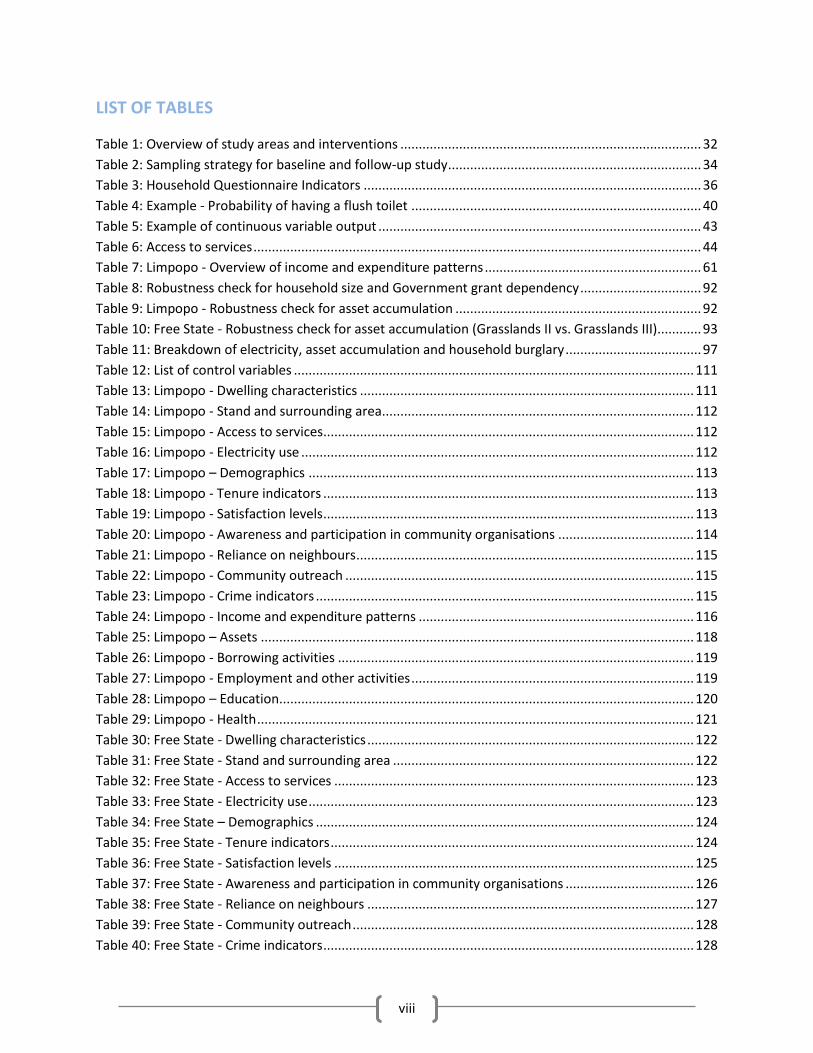
Figure 6: Probability chart ........................................................................................................................... 43

Figure 7: Limpopo - Structural characteristics ............................................................................................ 45

Figure 8: Typical Shack Dwellings in Disteneng .......................................................................................... 46

Figure 9: Poor road quality ......................................................................................................................... 47

Figure 10: Collecting water in Disteneng .................................................................................................... 48

Figure 11: Limpopo - Garbage disposal methods in control group ............................................................ 48

Figure 12: Limpopo - Source of lighting and cooking.................................................................................. 49

Figure 13: Limpopo - Distribution of household sizes ................................................................................ 51

Figure 14: Limpopo – Tenure-related outcomes ........................................................................................ 52

Figure 15: Limpopo - Significant differences in satisfaction levels ............................................................. 54

Figure 16: Limpopo - Reliance on neighbours ............................................................................................ 56

Figure 17: Limpopo - Awareness of Community Groups and Programmes ............................................... 57

Figure 18: Limpopo – Perception and actual crime rates ........................................................................... 59

Figure 19: Limpopo - Expenditure patterns ................................................................................................ 61

Figure 20: Limpopo - Prevalence of household appliances ........................................................................ 62

Figure 21: Limpopo - Unemployment and grant dependence ................................................................... 66

Figure 22: Limpopo - Morbidity rates by age .............................................................................................. 68

Figure 23: Free State - RDP houses in Grasslands II & III ............................................................................ 69

Figure 24: Free Sate – Bloemside ................................................................................................................ 70

Figure 25: Free State - Grasslands II & III .................................................................................................... 71

Figure 26: Free State - Probability of using the kitchen as a sleeping area ................................................ 72

Figure 27: Fencing around a shack .............................................................................................................. 72

Figure 28: Free State - Electricity use.......................................................................................................... 74

Figure 29: Free State - Tenure-based outcomes ......................................................................................... 76

Figure 30: Free State - Diverging satisfaction levels ................................................................................... 77

Figure 31: Free State - Similar satisfaction levels ....................................................................................... 77

Figure 32: Free State - Participation in community activities ..................................................................... 78

Figure 33: Free State - Reliance on neighbours .......................................................................................... 79

Figure 34: Free State - Perceptions of safety .............................................................................................. 79

Figure 35: Free State - Crime rates ............................................................................................................. 80

Figure 36: Free State - Expenditure patterns .............................................................................................. 82

Figure 37: Free State - Overview of assets .................................................................................................. 82

Figure 38: Free State - Household appliance accumulation over time ....................................................... 83

Figure 39: Free State - Employment and grant dependence ...................................................................... 84

Figure 40: Free State - Morbidity rates ....................................................................................................... 86

vii

Figure 41: Serviced Houses (Shacks and Upgraded Houses) in Chris Hani ................................................. 87

Figure 42: Gauteng - Household services ................................................................................................... 88

Figure 43: Gauteng - Government grants ................................................................................................... 89

Figure 44: Gauteng - Crime statistics .......................................................................................................... 89

Figure 45: Gauteng - Morbidity rates ......................................................................................................... 90

viii

LIST OF TABLES

Table 1: Overview of study areas and interventions .................................................................................. 32

Table 2: Sampling strategy for baseline and follow-up study ..................................................................... 34

Table 3: Household Questionnaire Indicators ............................................................................................ 36

Table 4: Example - Probability of having a flush toilet ............................................................................... 40

Table 5: Example of continuous variable output ........................................................................................ 43

Table 6: Access to services .......................................................................................................................... 44

Table 7: Limpopo - Overview of income and expenditure patterns ........................................................... 61

Table 8: Robustness check for household size and Government grant dependency ................................. 92

Table 9: Limpopo - Robustness check for asset accumulation ................................................................... 92

Table 10: Free State - Robustness check for asset accumulation (Grasslands II vs. Grasslands III)............ 93

Table 11: Breakdown of electricity, asset accumulation and household burglary ..................................... 97

Table 12: List of control variables ............................................................................................................. 111

Table 13: Limpopo - Dwelling characteristics ........................................................................................... 111

Table 14: Limpopo - Stand and surrounding area ..................................................................................... 112

Table 15: Limpopo - Access to services ..................................................................................................... 112

Table 16: Limpopo - Electricity use ........................................................................................................... 112

Table 17: Limpopo – Demographics ......................................................................................................... 113

Table 18: Limpopo - Tenure indicators ..................................................................................................... 113

Table 19: Limpopo - Satisfaction levels ..................................................................................................... 113

Table 20: Limpopo - Awareness and participation in community organisations ..................................... 114

Table 21: Limpopo - Reliance on neighbours ............................................................................................ 115

Table 22: Limpopo - Community outreach ............................................................................................... 115

Table 23: Limpopo - Crime indicators ....................................................................................................... 115

Table 24: Limpopo - Income and expenditure patterns ........................................................................... 116

Table 25: Limpopo – Assets ...................................................................................................................... 118

Table 26: Limpopo - Borrowing activities ................................................................................................. 119

Table 27: Limpopo - Employment and other activities ............................................................................. 119

Table 28: Limpopo – Education ................................................................................................................. 120

Table 29: Limpopo - Health ....................................................................................................................... 121

Table 30: Free State - Dwelling characteristics ......................................................................................... 122

Table 31: Free State - Stand and surrounding area .................................................................................. 122

Table 32: Free State - Access to services .................................................................................................. 123

Table 33: Free State - Electricity use ......................................................................................................... 123

Table 34: Free State – Demographics ....................................................................................................... 124

Table 35: Free State - Tenure indicators ................................................................................................... 124

Table 36: Free State - Satisfaction levels .................................................................................................. 125

Table 37: Free State - Awareness and participation in community organisations ................................... 126

Table 38: Free State - Reliance on neighbours ......................................................................................... 127

Table 39: Free State - Community outreach ............................................................................................. 128

Table 40: Free State - Crime indicators ..................................................................................................... 128

ix

Table 41: Free State - Income and expenditure patterns ......................................................................... 129

Table 42: Free State - Assets ..................................................................................................................... 132

Table 43: Free State - Borrowing activities ............................................................................................... 133

Table 44: Free State - Employment and other activities .......................................................................... 134

Table 45: Free State – Education .............................................................................................................. 135

Table 46: Free State - Health .................................................................................................................... 136

Table 47: Gauteng - Demographics ........................................................................................................... 138

Table 48: Gauteng - Economic indicators ................................................................................................. 138

Table 49: Gauteng - Health ....................................................................................................................... 138

Table 50: Gauteng - Services ..................................................................................................................... 139

Table 51: Gauteng - Education and Crime ................................................................................................ 139

x

ACRONYMS

AIDS Acquired Immune Deficiency Syndrome

ANC African National Congress

BNG Breaking New Ground

COHRE Centre on Housing Right and Evictions

DORA Division of Revenue Act

DWAF Department of Water Affairs

ECD Early Childhood Development

EPWP Expanded Public Works Programme

HIV Human Immune Virus

IDP Integrated Development Plan

IE Impact Evaluation

ITT Intention to Treat

LPM Linear Probability Model

M&E Monitoring and Evaluation

MDG Millennium Development Goals

MEC Member of the Executive Committee

NDOHS National Department of Human Settlements

PHP People’s Housing Process

PLM Project Level Monitoring

RDP Reconstruction and Development Programme

RICA Regulation of Interception of Communication Act

SAPS South African Police Service

TOT Treatment on the Treated

UISP Upgrading of Informal Settlements Programme

UN United Nations

1

EXECUTIVE SUMMARY

With the shift from Housing to Human Settlements, the National Department of Human Settlements

(NDOHS) has changed its focus from a purely quantitative approach (the number of houses delivered) to

a more holistic view of building sustainable communities. With the technical assistance of the World

Bank, the NDOHS has conducted a new series of rigorous impact evaluations to assess the effects of the

Upgrading of Informal Settlements Programme (UISP) interventions in Free State, Limpopo and Gauteng

Provinces. This is aimed at reliably identifying causal links between the rollout of the UISP and the

outcomes of interest driven by policy prescriptions (as well as broader concerns) for the programme. An

impact evaluation framework is being used to assess the programme’s effectiveness in obtaining its

policy objectives as well as influencing policy reviews resulting from the research findings.

Retrospective studies (based on interventions that have occurred in the past) were carried out in

Limpopo, Free State and Gauteng and the results from these three provinces are presented in this

report. In Limpopo, households were relocated from Disteneng and Greenside informal settlements

(Disteneng) on the outskirts of Polokwane to the nearby greenfield sites of Polokwane Extension 44 and

76 (Ext. 44/76) in 2006. This is a fully serviced and formalised area where the majority of households

have now been provided with subsidised homes (commonly referred to as RDP homes). The

Municipality’s decision to relocate all qualifying households to the West of the Disteneng dividing road

has resulted in a natural experiment where it is possible to compare households that were relocated to

households that remained in Disteneng in order to assess the impact of the relocation programme. This

study analyses the results from a survey of 1171 households consisting of 444 households in Ext. 44/76

and 727 households in Disteneng.

In Free State, a phased rollout of in situ RDP housing upgrades was conducted in the Grasslands

settlement on the outskirts of Bloemfontein, where Grasslands II residents were provided with housing

in 2006/2007 and Grasslands III followed in 2008/2009. Budget and planning difficulties meant that

sanitation was not provided to Grasslands households. Also, due to land acquisition delays, the

neighbouring area of Bloemside, which was also targeted for upgrading, had not been provided with

RDP houses at the time of the study. The area has, however, been formalised and residents provided

with fully serviced stands (water, electricity and sanitation). The phased rollout of the study and delays

in project plans due to land acquisition difficulties provides another natural experiment from which to

measure, retrospectively, the impact of the programme in Free State. A sample of 1014 households

consisting of 370 households from Grasslands II, 289 from Grasslands III and 355 from Bloemside was

used to generate the results in this report.

In Gauteng, an upgrading programme is currently being conducted in the Chris Hani Settlement in

Daveyton. The study area consists of 3 extensions, with extensive upgrading of housing, electricity and

sanitation occurring in Extension 3, with partial upgrading of houses and electricity in Extensions 1 and

2. The majority of households in all extensions have been provided with sanitation. The study exploits

the phased roll out of Extension upgrades to compare the extensively upgraded area of Extension 1 (398

2

household surveyed) to the partially upgraded areas of Extensions 2 and 3 where 905 households were

surveyed.

The chosen studies do not necessarily follow the UISP process guidelines and one can find in many cases

that projects across the country are initiating various forms of upgrading, often prioritising housing

(which is strictly meant to be the last step of the upgrading process) over other community upgrade

options. The study is not a process evaluation, and is thus not interested in whether or not the correct

steps have been taken in the upgrade process. Rather, the report is interested in understanding what

the implications of these variations are in terms of the impacts (intended and unintended) they have on

beneficiaries.

The study areas chosen allow for four comparisons. In Limpopo the design allows for estimating the

impact of relocating households from an informal settlement with no services (Disteneng), to a

formalised greenfield site with comprehensive services and supporting community facilities (Ext 44/76).

In Free State one is able to compare the relative impacts of being provided with a fully serviced stand

(Bloemside) to being provided with a partially serviced RDP house on the site of the original informal

dwelling (Grasslands). By exploiting the phased approach to the study, estimates can also be made on

the long-term impacts of being provided with an RDP home, by comparing Grasslands II residents who

have been living in their upgraded homes for three or four years to the neighbouring Grasslands III

residents who have had their RDP homes for one to two years. In Gauteng the impact of fully upgrading

an area compared to a partial upgrade (less than 50% households receiving housing and electricity) can

be estimated.

The results show strong impacts in household demographics, asset accumulation, social interactions,

satisfaction levels, household upgrading, crime rates, health and unemployment.

The most visible impact of upgrading from a shack to an RDP home is the change in the physical

characteristics of the dwelling. Households move from having an average of 1 bedroom in informal

shacks to an average of 2 bedrooms in an RDP home. This reduces the percentage of households that

use their kitchen as a sleeping area from 73% to 4% in Limpopo and 33% to 4% in Free State. In

Limpopo, where informal settlement dwellers do not have access to electricity, 90% of households use

paraffin and 9% use biomass for cooking. Paraffin lamps and candles are also widely used for lighting. In

Free State, most households in both areas have electricity, and it is noted that whenever electricity is

available, this is almost universally used for cooking and lighting (with the exception of a small

percentage of households that cook with paraffin instead). This high take up of electricity for cooking

and lighting is most likely the result of municipal subsidies (free basic electricity) in the study areas. The

results show that, in the absence of municipal waste removal, 25% of households in Limpopo and 28% of

households in Free State choose to burn their waste. The results indicate that the absence of services

can, combined, present serious health hazards for household members (indoor air pollution

exacerbated by poor ventilation and increased potential for uncontrolled fires) which may have acute

effects on children’s health, since they are the ones that will likely be required to sleep in the kitchen

area when space is limited.

3

While the report finds that child health is affected by the change in environment, these impacts are

not conclusive. In Limpopo child morbidity rates in the past month decrease from 40% in the informal

settlement to 26% in the formalised area, while overall morbidity rates (for all household members) is

roughly the same for both groups (21% and 23% respectively). However, in Free State the provision of

sanitation in the serviced stand outweighs the health benefits of an RDP home without integrated

sanitation. The morbidity rate for household members on serviced stands is 16% compared to 20% in

the RDP homes without sanitation. Child morbidity also decreases from 26% to 17%, although this

impact is not statistically significant.

There is strong evidence that providing houses on a serviced greenfield site in Limpopo shifts the

makeup of the household structure from one of a migrant labourer to a family unit. Household sizes

increase from 2 people in Disteneng to 4 people on average in the formalised areas of Ext 44/76.

Disteneng residents are more likely to be receiving child grants (34%) than have children stay with them

in their home (23%) whereas the opposite situation is observed for Ext 44/76 residents (55% receive

child grants and 65% have children staying with them). Household heads from Disteneng are also more

likely to have a spouse/partner who does not stay with them (46%) than their counterparts in Ext 44/76

(15%). Finally, it is noted that Disteneng residents spending approximately 11% of their total

expenditure on transfers to other households, while this is only 2% in Ext 44/76. These results highlight

the likelihood that informal settlement dwellers may choose to leave their families behind (possibly in

rural areas) while they search for work in the city, but will bring these family members to stay with them

when provided with better living conditions. There are small but insignificant differences in household

sizes in Free State (with both groups having comparable household sizes to Ext 44/76 in Limpopo),

suggesting that the provision of a serviced stand, or a partially serviced RDP home are both likely to have

similar effects on household heads’ decisions on whether or not to bring their families to stay with

them.

Shifts in household structures are likely to have far-reaching implications on a number of dimensions.

One such area is social interactions. The study measures household reliance on neighbours for medical

care, transport, child care, job opportunities, household services and food, and find Disteneng residents

are more likely than their counterparts in Ext 44/76 to rely on their neighbours across all of these

dimensions. Ext 44/76 residents are also more likely to participate in community organisations such as

neighbourhood improvement, volunteering and religious groups than Disteneng residents. Social

interactions thus shift from reliance on neighbours to support and upliftment of communities. In Free

State where there is little variation in household structures, there are also few strong relative impacts

on social interactions.

The increased tenure security that comes with the upgrading programme results in increases in the

likelihood that households upgrade their homes, take out loans, plan to use savings for upgrading

purposes in the future and obtain rental income through tenants. The percentage of households that

upgraded their home in the 12 months prior to the survey increased from 1% in Disteneng to 15% in Ext

44/76. In Free State, 6% of households in Bloemside’s serviced stands upgraded their homes while 14%

did so in the Grasslands RDP homes. This difference indicates that (1) households are more likely to

conduct upgrading when they are provided with an RDP home, and (2) the provision of serviced stands

4

is also likely to induce upgrading, but at a lower level. Households that have been staying on their stand

for a longer period of time (Grasslands II vs. Grasslands III residents) are less likely to have conducted

upgrading in the previous 12 months. This may be because upgrading has already occurred at an earlier

stage. Households with RDP homes are twice as likely to take out a loan in Limpopo as their

counterparts in the informal settlement, but this is not believed to be a result of increased property

rights since the use of their house as collateral for taking out loans is virtually non-existent. Instead,

smaller loans are being taken out (that do not require such large collateral), most often from

furniture/clothing/appliance stores to buy household goods.

Supporting the results on loan characteristics, the results show high levels of asset accumulation taking

place as a result of the interventions. Of the 23 assets measured, Ext 44/76 residents are more likely to

have 21 of these than their counterparts in Disteneng. The differences are greatest with assets requiring

electricity, such as TVs, fridges and microwaves. Since almost all households in the Free State groups

have electricity, the relative impacts on asset accumulation is minimal; however, there are significant

long-term impacts of staying in an RDP home. Grasslands II residents are significantly more likely to own

a microwave, fridge, oven, washing machine and iron than Grasslands III, illustrating how households

choose to invest in household goods over time. The acquisition of these goods has a number of positive

implications on household living conditions as they are able to store and cook food as well as save time

on household chores. While these are all positive results, it is important that this asset accumulation is

conducted in a sustainable way, since it is noted that household income across groups does not vary and

the acquisition of household goods is often done on credit.

Household income is roughly the same across all groups in both provinces, ranging from R1500 to R1650

a month. When considering per capita income, however, there are significant differences (especially in

Limpopo, given the large differences in household sizes). Increases in household size are not met with

commensurate increases in household income. In fact, unemployment rates increase for households

living in RDP homes. This report distinguishes between narrow and broad unemployment rates. These

are not based on the formal, standardised definitions, but are rather more simplified versions. This

report refers to a person that is unemployed but has actively looked for work in the past week as being

unemployed in the narrow sense. Broad unemployment considers all working-aged individuals that are

not working as unemployed. Narrow unemployment decreases from 23% in Disteneng to 18% (but not

statistically significant) in Ext 44/76. In Free State it rises from 15% in Bloemside to 23% in Grasslands.

Broad unemployment increases from 42% (Disteneng) to 56% (Ext 44/76) in Limpopo, and from 61%

(Bloemside) to 63% (Grasslands) in Free State. The large differential in narrow and broad unemployment

rates is well explained by household members that responded having “done nothing” as their main

activity in the previous week which is approximately 30% in Ext 44/76, Bloemside and Grasslands, but

17% in Disteneng. This highlights the problem of discouraged workers that are unemployed, but no

longer looking for work. This unemployment problem also manifests itself in household dependence on

Government grants, which rise from 17% in Disteneng to 34% in Ext 44/76 as a percentage of total

household income. It also rises from 22% in Bloemside to 28% in Grasslands. One potential reason for

this could be the decreased mobility that comes with providing a house. Informal settlement dwellers

5

are free to move to alternative areas of opportunity if they lose their job, but households provided with

a house are more likely to stay even if they lose their job (although this cannot be proven in this study).

Lastly, when comparing crime rates, perceptions of safety are improved with the provision of RDP

homes. Actual crime rates are also measured and broken into two categories: (1) Household burglaries

and (2) Other types of crime. In Limpopo, the crime rates for household burglaries remain the same

across groups at 19%, but there is a large impact on other forms of crime. The percentage of households

that have had at least one person fall victim of a crime (other than household burglary) decreases from

17% in Disteneng to 10% in Ext 44/76. The report also finds that most of these crimes occurred in the

home or settlement area (78% in Disteneng and 70% in Ext 44/76). In Free State the situation is

different. Household burglary decreases from 16% in Bloemside to 9% in Grasslands, but other forms of

crime are constant across groups (9%). Since dwellings are likely to be robbed depending on (1) how

secure the dwelling is and (2) what can potentially be stolen, asset accumulation is likely to partially

explain the household burglary results.

By using natural experiments in an impact evaluation framework, the results from this study can be

assumed to be causal impacts of the interventions evaluated. A number of caveats mean that the results

should be considered with caution. This report provides some recommendations based on the results,

but these are presented as general areas to guide the debate around effective methods of informal

settlement upgrading. As it stands, this study offers a set of results that can stimulate debate, but

prospective evaluations, looking at planned interventions, rather than interventions that have already

occurred will add more rigour and relevance to this evidence base as the NDOHS moves forward with

scaling up its efforts to rigorously estimate the causal impacts of its programmes to improve service

delivery over time.

6

1. INTRODUCTION

1.1. Background

In South Africa, slums and informal settlements have a distinctive history. During the apartheid years,

millions of blacks were forcibly removed from white areas and relegated to a life of poverty in

"homelands." Most blacks could not live legally in major South African cities, such as Cape Town or

Johannesburg. In order to support their families, many moved to illegal squatter settlements within

white areas or moved their families to "informal" shack settlements on a homeland's edge nearest to

white cities in order to have the shortest daily commute for work (Joyce, 2003).

Free-standing informal settlements arose in South Africa during the 1970s and 1980s as a result of the

collapse of apartheid influx controls. Many of these settlements were originally earmarked for

demolition, with a view of relocating residents to more peripheral sites. Communities resisted the

relocation and this resulted in the formation of strong community organisations. Around 1980, the

apartheid government had largely abandoned its “black spot” removal policy. Population densities

within existing black formal residential areas increased dramatically and the demand for

accommodation led to the extensive developments of backyard shacks for rental purposes.

The post apartheid South African state managed to lift apartheid restrictions which resulted in the

promulgation of new urban policy. Legislations, such as the Housing White Paper of 1994, Constitution

of the Republic of South Africa 1996, Housing Act of 1997, Housing Code of 2000, Breaking New Ground

(BNG) of 2004, of improving the lives of slum dwellers, were promulgated.

Other policies and legislations were enacted largely to redress apartheid inequalities. As a result rapid

urbanisation is taking force as cities are experiencing high population growth, congestion, deteriorating

environmental quality and the increasing cost of urban services. These increased living costs are also not

necessarily offset by the potential for increased earnings that many see the cities as being able to

provide, noted by Godehart and Vaughan (2008): ‘Migration to urban cities and internal growth of cities

exceeded by far the creation of jobs’. There is a view that the urbanisation rate is very likely to reach

about 75% by 2020 in South Africa (Berrisford, 1998).

The National Department of Human Settlements (NDOHS), previously known as the National

Department of Housing initiated the ‘Upgrading of Informal Settlements Programme’ (UISP), under a

broader policy “Breaking New Ground.” The main aim of this programme is to facilitate the structured

incremental upgrading of informal settlements in cases where this is possible. Where this is not deemed

possible, and as a last resort, the programme includes cases where communities must be relocated. Its

main aims are to promote tenure security, health and welfare and community empowerment amongst

those residing in informal settlements. Questions remain as to how best to achieve these objectives in

different circumstances, and understanding the impact UISP has on beneficiaries in its various

implementation forms is key to improving and directing the programme as it moves forward.

To account for its broader mandate, the NDOHS shifted its focus from a purely quantitative approach

(the number of houses delivered) to a more holistic view of building communities. With the technical

7

assistance of the World Bank, the NDOHS is leading a new programme of rigorous impact evaluations to

assess the effects of the UISP interventions in the provinces of Free State, Limpopo and Gauteng. This is

aimed at reliably identifying causal links between the rollout of the UISP and the outcomes of interest

driven by policy prescriptions (as well as broader concerns) for the programme. An in-depth impact

evaluation is required to assess the programme’s effectiveness in obtaining its policy objectives as well

as influencing policy reviews resulting from the research findings.

1.2. Motivation for the Study

Government departments implement a number of projects and programmes across the country. It is

often difficult to isolate the effect of one particular programme, making it hard to know where

programmes are working and where changes are needed. While billions of Rands are being spent

annually on various programmes, it is critical to understand how effective they are in achieving their

ultimate objectives. A deeper understanding of these effects (both intended and unintended) can

improve planning and efficiency of resource allocation. Therefore the NDOHS has initiated a national

round of impact evaluations to accurately assess what the impact of the UISP has had on its

beneficiaries in order to determine its effectiveness. The study aims to support evidence-based policy,

where decisions are made based on empirical evidence of what does and does not work.

1.3. Objectives of the Study

The main objectives of the study will be to rigorously measure the impact of the UISP on the welfare of

local communities across a broad range of indicators, and (in future rounds of the study) investigate

whether specific interventions or combinations of interventions are more cost-effective than others in

achieving positive outcomes. Evidence generated through the impact evaluation will be used to provide

recommendations that can strengthen the programme’s effectiveness over time.

The first objective can be measured in the current baseline study; however, only after joining a number

of similar studies in the future that will be conducted in nine provinces, tracking changes over time, can

the second objective can be met. By assimilating the results from the different provinces, the bigger

picture will be able to determine where the UISP has worked, where it has faced challenges and where it

can improve in meeting its objectives over time. These studies will also hopefully highlight a broad range

of intended and unintended impacts that will help in determining not only whether or not the

programme is achieving its stated objectives, but also where the programme can improve its delivery

and what household and community dynamics can be expected when the UISP is implemented.

1.4. Monitoring and Evaluation

Monitoring and evaluation (M&E), from inputs to impact is usually considered within the logical

framework (logframe) model.

While monitoring is chiefly concerned with inputs and outputs, impact evaluations looks further into

what is the resulting impact of the UISP on the lives of the beneficiaries.

8

The Chief Directorate: Monitoring and Evaluation has the mandate to monitor and evaluate the

performance of all National Human Settlements Programmes applicable in all nine provinces.

Monitoring is done through project-level monitoring exercises. The rationale for project-level

monitoring (PLM) is to:

verify the performance of Provincial Human Settlements Departments against the set

targets;

identify challenges in the performance of housing projects at implementation level, and

make recommendations to address them;

record measures undertaken by the Provincial Department and/or the Municipality

implementing the projects, in addressing the challenges and obstacles identified in the

projects; and

record and document best practices on the implementation of the various housing

programmes.

Figure 1: Monitoring and evaluation framework

(Bennett & Rockwell, 1995).

Housing delivery is critical, but it is a means in which to meet the ultimate ends of improving the lives of

beneficiaries and building sustainable settlements. Monitoring sets the basis for measuring delivery

progress; however, when you want to go beyond merely recording the current state of programmes, to

9

measure what the impact of these programmes has been and critically analyse what is working, what is

not working and why this might be the case, monitoring is limited. Impact evaluation (IE) measures the

UISP effects on beneficiaries and the extent to which its goals and objectives are being attained. It helps

generate knowledge in critical development areas and find evidence-based solutions to the most

pressing concerns, such as how to expand access to services such as water, sanitation, electricity, health,

and quality education in a cost-effective and efficient manner. IE moves away from the assumptions

about what might work, towards generating evidence of what does work. In essence, the aim of IE is to

measure the causal effects of a programme, and in so doing generate a body of knowledge to inform

policy decisions and programme design (Afedorova, 2010)

The rationale for IE is to

determine whether the projects implemented in provinces had the desired effects on

individuals, households and institutions;

understand what other effects the programme may have had, other than those based on the

stated objectives; and

understand whether those effects are directly attributable to the projects.

While monitoring is concerned with inputs and corresponding outputs, evaluation focuses on impacts

and outcomes while considering the causal links to project objectives from outputs and the inputs

intended to produce them through project processes and given specific assumptions.

1.5. Outline of the Report

This report provides a literature review in Section 2 covering the relevant legislative framework, current

academic findings on the effects of housing and services on beneficiaries and an overview of the current

UISP framework. The report will continue with a detailed look into the specific study areas in Section 3,

before describing the methodology used in the study in Section 4. A briefing on how to interpret the

results is included in Section 5, followed by the detailed results of the study presented in Sections 6, 0

and 8. After this, the reliability of the results is put into context by conducting robustness checks and

highlighting caveats in Section 9. The report closes with reflections and recommendations in Section 10

and concluding remarks in Section 11.

10

2. LITERATURE REVIEW

This chapter starts with framing the current delivery of Government housing within the context of the

legislation that has preceded it in the past 16 years, tracking the shifts in mindset over time. It then

provides an overview of the UISP policy itself and which components of this policy the study addresses.

Following this, it considers some of the current challenges in housing delivery and finishes with a look

into what previous research has been able to identify in terms of benefits accruing to beneficiaries of

housing programmes, basic services, relocation and improved tenure security and which have served to

direct the study hypotheses ex ante. It is believed that the work from this study can contribute to the

current knowledge base in these areas as well as provide insight into the dynamics related to the

provision of houses and services that can ultimately benefit and refine the UISP policy moving forward.

2.1. Legislative Prescripts and Policies

The Constitution of the Republic of South Africa

The Constitution of South Africa, Act 108 of 1996 defines the fundamental values, such as equality,

human dignity, and freedom of movement and residence, to which the housing policy must subscribe. In

terms of Section 26 of the Constitution every citizen has the right to have access to adequate housing.

The state is required to take reasonable legislative and other measures, within its available resources, to

achieve the progressive realisation of this right. Furthermore, the constitution states that no person may

be evicted from their home, or have their home demolished, without an order of court made after

considering all the relevant circumstances. No legislation may permit arbitrary evictions. Section 25 of

the Constitution states that government “must take reasonable legislative and other measures within its

available resources, to foster conditions which enable citizens to gain access to land on an equitable

basis.”

The Housing Act

In 1997 the Housing Act (Act No. 107 of 1997) was promulgated resulting in the legislation and extension

of the provisions set out in the White Paper of 1994 on Housing. This gave legal foundation to the

implementation of government's Housing Programme. The Housing Act aligned the National Housing

Policy with the Constitution of South Africa and clarified the roles and responsibilities of the three

spheres of government: National, Provincial and Municipal.

Section 2(1) (a) of the Housing Act, 1997 (Act No. 107 of 1997) compels all three spheres of government

to give priority to the needs of the poor in respect of housing development. In terms of the Housing

Amendment Act 4 of 2001, Section (1) the Minister is responsible to (i) evaluate the performance of the

housing sector against set goals and equitableness and effectiveness requirements and (ii) take any

steps reasonably necessary to create an environment conducive to enabling provincial and local

governments, the private sector, communities and individuals to achieve their respective goals in

respect of housing development and promote the effective functioning of the housing market.

Monitoring the performance of housing programmes is mandated through Section 9(1) of the Division of

Revenue Act (DORA), and the Housing Act, 1997 (Act 107 of 1997). The Housing Act, Section 3(2)

11

mandates the Minister to monitor the performance of the NDOHS’ programmes and in cooperation with

every member of the executive council (MEC), the performance of provincial and local governments

against housing delivery and budgetary goals. Chapter 5 of the National Treasury Regulations stipulates

that the Accounting Officer of an institution must establish procedures for quarterly reporting to the

executive authority to facilitate effective performance monitoring, evaluation and corrective action.

The National Housing Code

According to the revised National Housing Code of 2009 there are six incremental interventions

programmes delivered through the NDOHS, namely the Consolidation Programme, Emergency

Programme, Integrated Residential Development Programme, Enhanced People’s Housing Process,

Informal Settlements Upgrading Programme and Quantum - Incremental Interventions.

In terms of the revised Housing Code of 2009, the UISP deals with the process and procedure for the in

situ upgrading of informal settlements as it relates to the provision of grants to a municipality to carry

out the upgrading of informal settlements within its jurisdiction in a structured manner. The grant

funding provided will assist the municipality in fast tracking the provision of security of tenure, basic

municipal services, social and economic amenities and the empowerment of residents in informal

settlements to take control of housing development directly applicable to them. The Programme

includes, as a last resort, in exceptional circumstances, the possible relocation and resettlement of

people on a voluntary and co-operative basis as a result of the implementation of upgrading projects.

Comprehensive Housing Plan for the Development of Integrated and Sustainable Human Settlements

commonly known as the Breaking New Ground (BNG) strategy

In September 2004 Cabinet approved the Breaking New Ground Strategy (Comprehensive Housing Plan

for the Development of Integrated Sustainable Human Settlements). The new human settlements plan

reinforces the vision of the NDOHS to promote the achievement of a non-racial, integrated society

through the development of Sustainable Human Settlements and quality housing. The strategy further

emphasises that, in order to assess the relationship between the housing sector and macro economy in

South Africa, the analysis of the intersection of the housing sector with the broader economy can be

desegregated into four interrelated areas:

Real side linkages: Real linkages include the effects of housing policy on such macro economic

variables as output, employment, income, consumption, savings and investment, prices,

inflation, and the balance of payments;

financial linkages: Financial linkages deal with the relationship between the financial sector - in

particular formal and informal institutions providing housing finance – and the demand for, and

supply of, housing;

fiscal linkages: Fiscal linkages cover the contribution of government to the supply of housing

through tax and subsidy policy; and

12

socio-economic linkages: Housing policy, through the quantum and quality of housing delivered

impact on socio-political stability, productivity and attitudes and behaviour.

Understanding these linkages requires looking beyond the delivery of houses to the knock-on effects of

what this delivery impacts on. The study focuses mostly on the real-side (at the micro level) and socio-

economic linkages. Although this is a micro-level study, it is hoped that, through the integration of

similar projects across the country it will be possible to start building a micro base that can ultimately

inform the likely macro benefits of the UISP.

The BNG shifts the strategic focus of housing policy from the simple delivery of low cost housing to the

delivery of low cost housing in settlements that are both sustainable and habitable. Through this policy

shift, the NDOHS is:

emphasising the development of social housing options;

implementing inclusive housing policy requirements;

promoting the upgrading of informal settlements; and

simplifying the administration of the housing subsidy programme and extending the reach of

this programme.

Some of the transformative aspects of the Breaking New Ground policy on informal settlements include:

in situ upgrading of informal settlements;

making funding for land rehabilitation available;

encouraging local municipalities to purchase well-located land that is occupied or unoccupied;

making provision for household support in the case of relocation;

creating provision of social and economic facilities and infrastructure development;

funding the provision of basic infrastructure; and

encouraging permit/permission to occupy forms of tenure.

The BNG policy is ambitious and requires an M&E support structure to measure the attainment of its

objectives. Measuring the number of houses constructed is no longer enough, and a much more holistic

assessment of programmes needs to be considered to complement the innovative policy. This UISP

impact evaluation is a first step towards quantifying the effects of BNG across a number of “softer” (but

still critically important) outcomes such as income levels, employment, investment, health, savings and

child development. Promoting these “lifestyle outcomes” is critical to the success of a sustainable

housing programme. How to go about doing this requires an in-depth look at the UISP programme itself

to compare this to what is happening on the ground.

Millennium Development Goals

The Government of the Republic of South Africa is a member of the United Nations Millennium

Development Goals (MDGs), which seek to provide significant improvement to the lives of at least 100

million slum dwellers by 2020. Therefore, the UISP is consistent with this convention with its primary

aim of catering for the special development requirement of informal settlements. Through its

13

implementation the UISP can also indirectly pursue other MDGs such as: (1) Eradicate extreme poverty

and hunger, (2) Achieve universal primary education, (3) Promote gender equality and empower

women, (4) Reduce child mortality, Improve maternal health, (5) Combat HIV/AIDS and other diseases

and (6) Ensure environmental sustainability. In this light, it is clear that the UISP plays a crucial role in

achieving global development objectives, and this study is a stepping stone into understanding to what

degree it is able to effect change across these myriad development opportunities.

2.2. Upgrading of Informal Settlements Programme: A Primer

The National Housing Code sets out the national approach to informal settlement upgrading in a

structured manner. Chapter 13 of the National Housing Code introduces the objectives of the UISP:

“The challenge of informal settlements upgrading must be approached from a pragmatic perspective

in the face of changing realities and many uncertainties. Informal settlements should also not be

viewed as merely a ‘housing problem’, requiring a ‘housing solution’ but rather as a manifestation of

structural social change, the resolution of which requires a multi-sectoral partnership, long-term

commitment and political endurance. At the outset therefore, a paradigm shift is necessary to

refocus existing policy responses towards informal settlements from one of conflict or neglect, to one

of integration and co-operation” (Department of Housing, 2005:45).

It is clear from the above statement that the way in which informal settlements are addressed

(upgraded) by Government requires integrated thinking and improvisation. Rather than “eradicating

informal settlements by 2014” by converting shacks into houses the UISP aims to integrate and

formalise informal settlements through a number of instruments that lead to the structured incremental

upgrading of these settlements.

Objectives of the UISP

This programme promotes the upgrading of informal settlements to achieve the following complex and

interrelated policy objectives:

Tenure Security: recognising and formalising the tenure rights of the poor residents within informal

settlements wherever feasible. This process seeks to increase access and use of physical land assets

in the hands of the urban poor, reducing their vulnerability and enhancing their economic

citizenship and capability. Tenure security is also intended to normalise the relationship between

the state and the residents of informal settlements;

Health and safety: promoting the development of healthy and secure living environments which will

in turn restore dignity to the urban poor; and

Empowerment: specifically addressing social and economic exclusion by focusing on community

empowerment as follows:

o Social development – through the provision of social services such as primary- and

municipal-level social amenities and community facilities such as sport fields, community

14

halls etc. to serve the needs of the residents of informal settlements. In addition, creating a

platform for the future delivery of secondary and tertiary social services such as schools,

hospitals and police stations;

o Economic development - by directly facilitating the development of municipal-level

economic infrastructure such as transportation hubs, workspaces and markets. The

programme also supports job creation in so far as it works with the grain of the Expanded

Public Works Programme (EPWP). Urban efficiency will also be enhanced and the Urban

Renewal Programme supported; and

o Social capital – through encouraging the development of social capital by supporting the

active participation of communities in the design, implementation and evaluation of

projects. Additionally, the programme aims to enhance social networks in order to reduce

household vulnerability, and improve security and community belonging.

UISP principles and guidelines

The programme promotes engagement between local authorities and communities living within

informal settlements. It also ensures that communities are upgraded in a holistic, integrated and locally-

appropriate manner. The community must be informed and it must approve where communities will be

relocated (when this is seen as the only option) and the new location must be part of an approved

Integrated Development Plan (IDP) of the municipality. The programme is generally implemented in a

phased approach, with four key stages, namely: (1) The application phase: Here the local municipality

will be funded if the business plan (which should contain all the necessary pre-feasibility information

about the project) is successful; (2) The project initiation phase: This is where negotiations with land

owners and registration of properties take place. This phase includes an assessment of the geotechnical

and other environmental conditions and installation of interim services; (3) The project implementation

phase: Here, a full business plan is submitted and support is given to formalising occupational rights and

disputes, developing municipal infrastructure and providing social amenities and community facilities;

and (4) The housing consolidation phase: Here beneficiaries are provided with housing and any

outstanding community facilities/amenities are built to finalise the upgrading process.

It is clear, when considering the incremental process that UISP purports, that housing delivery itself is

only one (and generally the last) piece of the upgrading puzzle. The view is one of a holistic incremental

upgrading that includes, among others, the following support:

Service standards: programme provides funding for the installation of interim and permanent municipal

engineering services. The nature and level of permanent engineering infrastructure must be the subject

of engagement between the local authority and residents. The installation and maintenance of services

must be undertaken in accordance with the principles of the Expanded Public Works Programme to

maximise job creation.

Social and economic amenities: the programme makes funding available for the construction of limited

social and economic infrastructure. The determination of the type of infrastructure to be developed

15

must be undertaken through a process of engagement between the local authority and residents. The

community needs must be assessed prior to the determination of community preferences. Funding for

maintenance and operation must be provided from non-housing sources by the municipality.

Tenure: the programme promotes security of tenure as the foundation for future individual and public

investment. The broad goal of secure tenure may be achieved through a variety of tenure arrangements

and these are to be defined through a process of engagement between local authorities and residents.

The selected tenure arrangement must protect residents against arbitrary eviction.

Community Partnership: the programme promotes active community participation. The funding is

accordingly made available to underpin social processes. Community participation is to be undertaken

through the vehicle of Ward Committees or a similar structure where Ward Committees don’t exist, in

line with the provisions of the Municipal Systems Act; All key stakeholders must be included within the

participatory process; The municipality must ensure that effective community participation has taken

place in the planning, implementation and evaluation of the project; and Special steps may be required

to ensure the ongoing involvement of vulnerable groups.

Demolition of shacks: the municipality will be required to table a comprehensive action plan for the

management of projects specifically addressing measures to prevent land re-invasion and the processes

of shack demolition when persons access phase four benefits and receive permanent houses.

The chosen studies do not necessarily follow the UISP process guideline and it is noticeable in many

cases that projects across the country are initiating various upgrading forms, often prioritising housing

(which is meant to be the last step of the upgrading process) over other community upgrade

components. This study is not a process evaluation, and is thus not preoccupied with whether or not the

correct steps have been taken in the upgrade process, but rather, it is interested in understanding what

the implications of these variations are in terms of impacting the livelihoods of the beneficiaries.

UISP Beneficiaries

In order to qualify for a housing subsidy beneficiaries must have a household income of not more than

R3 500 per month, must not have owned a fixed residential property previously, must be married or

single with dependants and must be a lawful resident of South Africa.

In general UISP will apply to the upgrading and/or development of informal settlements that typically

manifest themselves in the following ways:

Illegality and informality – the residents of informal settlements live in a state of legal-social

insecurity as these settlements lack legal recognition due to the unlawful occupation,

unauthorised use of land and/or the illegal construction of houses upon land. Primarily as a

result of their illegal status, most informal settlements are characterised by the absence of

formal planning and incremental, unplanned growth;

16

Poverty and vulnerability – since inhabitants of these settlements are mostly poor with basic

educational qualifications, they are typically dislocated from the formal labour market. The

inhabitants are also vulnerable to high-risk diseases and possible loss of lives due to their poor

living circumstances; and

Social stress and crime - the informality of settlements, including high densities, the absence of

demarcated roads, poor lighting and under-developed public open space, provides an ideal

space for criminal activities. Poverty in these settlements provides fertile ground for social stress

which can manifest itself in high levels of inter-personal crime including domestic violence, child

abuse and various social pathologies.

While implementing this programme, full cognisance needs to be given to the major challenges with

housing delivery in general.

2.3. Challenges with Housing Delivery

This section considers three key challenges associated with housing delivery, namely, rapid urbanisation,

population growth and employment.

Rapid urbanisation

For the first time in South African history, more people now live in cities than in the rural areas. While

the urban population is also growing by 5.8% per annum, a huge number of urban poor households live

in insecure, impoverished conditions and cities are unable to respond adequately to the growing

demands of urban growth (NDOHS, 2009b).

Mahanga (2002) adds that basic infrastructure services such as water supply and accessibility to urban

centres are in a dismal state. Likewise, overcrowded housing, unemployment and urban poverty have

also been growing. It is vital to note that most informal settlement inhabitants migrate from the

countryside to flee from rural poverty, seeking relative progress amidst the seeming optimism of

cosmopolitan opportunities (Kramer, 2006). Moreover, migrants are attracted to cities by socio-

economic conditions such as the considerable rural-urban gap of living standards (Lai, 1995).

The pull factor of better access to socio-economic opportunities contributed to the establishment, if not

the permanence, of informal settlements in South Africa. Like in Tanzania, ‘deficiency in housing supply

remains a critical problem to cater for this rapid urban expansion’ (Magigi and Majani, 2006:3/24). This

is evident when observing the challenges that Government faces in trying to reduce the housing

backlog, which currently stands at approximately 2.1 million houses (Need for Adequate Shelter (NDoHS

Estimate 2010/11).

However, migrants lack the ability to succeed in the cities due to lack of skills, education and decent

houses (Yap, 1995). They often ‘become victims of the city’s wrath’ and ‘they pose a daunting problem

to policymakers in the developing world’ (Atuahene, 2004: 1110). The reality is that migrants frequently

live in informal settlements that are ‘economically, socially, and politically marginalised urban

communities’ (ibid: 1110). This lack of skills also affects their ability to sustain their livelihoods.

17

It is as a result of urbanisation that government is faced with a challenge of informal settlements

especially in big cities. These informal settlements are characterised by poor service delivery, lack of

secure tenure, access to formal housing and land, safety and security and environmental hazards.

Population growth

South Africa has a high rate of population growth that is impacting on the cities in the form of

burgeoning squatter camps and informal settlements (Saff 1993:235). In 1994 approximately 1.06

million households comprising 7.7 million people lived in informal settlements, and an estimated 720

000 serviced sites that were provided by provincial legislatures under the previous government required

upgrading (Republic of South Africa 1994:9, South African Institute of Race Relations 1994: 328,367,

Barry and Mason 1997).

According to Statistics South Africa’s estimates, in 2007, there were 1.2 million households (9.7% of

South Africa’s estimated 12.5 million households) residing within informal settlements despite the

concerted effort made by Government to ease the backlog by providing approximately 2.5 million

houses in addition to 750 000 serviced sites over the past 16 years of democracy. This reality addresses

the important question: Should Government be focusing on ‘eradicating’ or integrating informal

settlements by 2014, given the seemingly insatiable demand for new housing? It is clear that, with

limited resources the housing backlog presents a massive challenge requiring efficient and effective

planning and implementation. Understanding the most effective way to achieve the UISP’s outcomes of

interest is thus not only desirable, but also critical to the Government’s current development plans.

Unemployment

According to the New Housing Policy and Strategy for South Africa (2008), South Africa is characterised

by large scale unemployment in the formal sector of the economy. While skilled labour is in high

demand, there is a mismatch between the demands of the country and the labour force (which consists

predominantly of unskilled labour). The increasing growth rate of the unskilled, but economically active

population implies that the level of unemployment is set to increase still further. The high level of

unemployment has a negative effect on demand for, and investment in housing and diminishes

Government's resource ability to assist the poor and unemployed. A solution to this problem is

fundamental to a sustainable solution for the housing problem.

The housing sector has a potentially large role to play in increasing demand for labour and improving the

economy through the direct and indirect economic multiplier effect of housing production. However,

the question remains – can this be a sustainable solution? While expanded public works programmes

are critical for generating labour and consumption demand, are there any direct effects of the provision

of housing on the labour choices and market attractiveness of housing beneficiaries? The report turns to

previous literature to find a starting point on which to explore this and other questions asking what

contribution housing programmes can provide to the economic and social lives of their beneficiaries.

18

2.4. Housing Programmes and their Effects

Housing

Informal settlements are home to millions of the urban poor households across developing countries

and represents the only option for millions of these families (UNCHS, 1999). Most of the households in

these areas represent the poorest of the urban population while their conditions and facilities replicate

their own and their country’s poverty and inequalities (Mahanga, 2002). In addition to the difficult living

conditions, there is a very strong shared and reinforced relationship between housing, poverty and the

environment. Thus, housing can be seen to have intrinsic value (good housing in and of itself is

important), but to understand its full benefits it is important to be cognisant of its instrumental value

too – ie. What role housing plays in affecting other dimensions of one’s life (health, security,

productivity etc.)?

Martin (1983) identifies some key benefits of settlement upgrading:

Health: minimise risks of epidemics;

Economic: empower local communities;

Social: integrated social support through the development of amenities like clinics; and

Tenure security: a legal tool to increase tenure security for the urban poor

Classic upgrading schemes in the international perspective ‘provide footpaths and latrines, street

lighting, drainage and roads, often water supply and limited sewerage’ (Chattopadhyay, 2009; UN-

Habitat, 2007:2). Settlement improvement involves regularisation of the rights of land, housing and

upgrading of the existing basic services. It does not necessarily consist of a home construction but it

‘offers loan options for home improvements’ as well (UNHabitat, 2007:2). Upgrading often involves

other actions such as the removal of environmental hazards, empowering communities through

maintenance and the building of communal facilities such as schools and clinics. This talks to a holistic

perspective of settlement upgrading where the physical dwellings themselves play one part in the bigger

picture.

The stated goal of the South African government is to overcome this housing backlog by 2014; but

doubling the budget will achieve this by only 2030 (Romano and Hensher, 2009). Current policy is to

deliver a choice of housing alternatives, but in practice 'a house on a fully serviced property with

freehold title' is seen as the only alternative. A new model estimates the value that residents of an

informal settlement place on aspects such as level of municipal engineering services, location and type

of upgrade, and the size of the dwelling. The model was applied to three issues in the current debate on

informal settlement upgrading in South Africa, namely: (1) whether to upgrade by relocating all

residents to a 'greenfield' site or upgrading in situ? (2) Whether to upgrade incrementally across many

settlements or upgrade fully one settlement at a time? (3) Whether to offer residents more than one

upgrade alternative? The stated choice approach provides a method to develop and test many housing

alternatives as part of involving the community in the upgrading of an informal settlement (Romano and

Hensher, 2009). The study adds to work such as this by highlighting the instrumental value of housing as

19

it is delivered in myriad ways. By building an evidence base, the NDOHS will be able to answer questions

such as these using a more informed approach.

Despite the vast resources spent on housing, little is known about the causal effects of such

interventions on health and other development outcomes of interest. The existing literature consists of

primarily cross-sectional descriptive studies, with few randomised studies. An exception is Katz et al.

(2001), who study the welfare outcomes of families living in poor urban areas that received housing

vouchers through a random lottery in the U.S. They find that the programme led to improved health for

children and adults. Furthermore, most of the development literature on informal settlement upgrading

is focused on Latin America, with no cases evident in Africa. In Peru, using non-experimental methods,

Field (2004) finds that an urban land titling programme led to large increases in housing investment.

Similarly, Galiani and Schargrodsky (2005) use a natural experiment that led to a random allocation of

land titles in an Argentinean city and find that the awarding of property titles yield significant housing

improvements, lower household size, and also lead to increases in children’s education attainment and

reductions in the number of school days missed. The authors estimate that the benefits in terms of

improved school performance was comparable to PROGRESA/Oportunidades, a major program of the

Mexican government aimed at developing the human capital of poor households through cash transfers

conditional on household investments in education and health. In a quasi-experimental study, Cattaneo

et al. (2007) use a Mexican government programme (Piso firme), replacing dirt floors by cement floors

and find large positive impacts on various child health measures (reduction in parasitic infections,

diarrhoea, anaemia), cognitive development and adult mental health and happiness. Rigorous studies

exploring the effects of housing on other key indicators such as security, social cohesion and

employment are lacking, and this paper hopes to address the gap.

The Department of Human Settlements finds itself in a unique position as a hub for multiple

Government Departments and programmes. Sustainable human settlements are where health, security,

education, social development, transport, basic services and land reform (among others) meet to

provide an integrated solution to improving the lives of the urban poor. The UISP thus does not focus

just on top structures per se, but a major component of the programme includes improved access to

basic services. But where should the priorities lie? This is a question that should be answered by asking a

slightly different question: What are the relative impacts of different packages of provisions? Priorities

should then be based on maximising impact.

UNCHS (1999) asserts that by tackling the issue of security of tenure and access to basic services and

decent housing, the settlement upgrading and incorporation into the overall structure of the city is a

necessary step towards more equitable and liveable cities. This means that upgrading efforts are not

only shown to have the ability to construct new models and paradigms of urban inclusion and planning,

but upgrades also need to be seen as a sensible mode to face the challenges of urbanisation and poverty

eradication across the cities of developing countries. There is also an assumption that upgrading would

alleviate the constraints on community efforts and offer the necessary support to improvements,

without disrupting social or economic links, but a stronger evidence base is needed to fully support

these assumptions.

20

Access to Services: Water, Sanitation and Electricity

Beyond the physical structure, upgrading also usually addresses improvement of services. Experience

has shown that access to basic services, and a house provides a foundation for households to improve

their social and economic circumstances (Housing Project Process Guide, September 2009). Even where

people are housed, conflicts continue over access to basic services and housing payments. Reports

regularly appear in the South African press of the formation of committees of township residents

occupying unoccupied houses, and fighting the cut-off of water and electricity for non-payment (Knight

2001).

According to the Department of Water and Forestry (DWAF), 86% of all households in South Africa have

some form of water provision, even if it is a stand pipe up to 200m away (BBC News, South Africa 2009).

Between 1994 and 2000 in South Africa, 1.5 million new electricity connections were established and 4

million more people given access to clean running water. Many of these connections are for a special

kind of pre-paid meter. This means that many people are now able to use electricity for basic activities

such as cooking as well as lighting. However, many people have been unable to afford to pay for these

services. A survey by USAID found that South Africans were willing but unable to pay for services

(Knight 2001). This raises the important question of whether, after the provision of electricity,

households are fully utilising their services. Are their financial constraints limiting its usage? When

considering the current and proposed tariff hikes from Eskom, will people be able to afford to use this

service after the electricity grid has been extended to their households, or will they require further

subsidies, increasing the burden on Municipalities as a result of non-payment?

During the 1999 election campaign the ANC promised to provide free electricity and water to the

poorest households. However, it is expected to take some time before this promise can be fully met.

Addressing the sanitation backlog was one of the first priorities of the newly elected democratic

Government in 1994. On 1 July 1994, a new Department of Water Affairs and Forestry (DWAF) was

established that consolidated government staff from all parts of the previous structures into one new

organisation. In the absence of a coherent policy for water supply and sanitation, the White Paper on

Water Supply and Sanitation Policy (DWAF, 1994) was compiled that set out the policy for the new

Department with specific regard to these services.

Another 15 million people live in local government areas where the local government has not decided to

implement the DWAF water policy or are in the process of doing so. In 2001, an estimated seven million

people live in areas where there was no infrastructure for the supply of water (Knight, 2001).

At the beginning of 2001 the national backlog of persons without access to adequate sanitation facilities

was estimated to be 18 million, or 3 million households. The majority of people falling into this category

live in rural areas, peri-urban areas and urban informal settlements. It was estimated that up to 26% of

urban households and 76% of rural households had inadequate sanitation in 2001 (Knight, 2001).

Significant investments are being made in the provision of safe water supplies for all. However, the

health benefit of this investment is limited where inadequate attention is paid to sanitation and to

health and hygiene promotion. International experience shows that once people’s basic needs are met

21

(especially the provision of clean water), sanitation improvements together with health and hygiene

promotion results in the most significant impact on their health.

Sanitation programmes can have dramatic health benefits because many of the infective organisms are

spread from hand to mouth or from hand to food to mouth rather than through drinking contaminated

water. Improving hygiene practices and providing sanitation facilities could have a direct influence on a

number of important public health problems besetting South Africa. Thus, understanding how infections

are transmitted and how to break the cycle of infection are important public health messages (Magalies

Water, 2009).

Bacteria, viruses and parasites found in human waste are responsible for the transmission of cholera,

typhoid and other infectious diseases that kill thousands of people every year. Approximately 90% of

these deaths are children. This not only affects individual’s health and daily lives but is one of the most

effective ways of promoting economic growth, education and equity issues. The provision of sanitation

is not only important in terms of improving peoples’ daily lives but is one of the most cost effective ways

to help improve the economy, health, education and help address equity issues.

An extensive electrification programme has been implemented throughout South Africa since 1994.

According to available statistics from the National Electricity Regulator and the Department of Minerals

and Energy, the level of electrification in South Africa has risen from 36% in 1994 to 71% at the end of

2004. Although there are slight discrepancies, the electrification trend is further highlighted in the

Statistics South Africa (StatsSA) 2009 General Household Survey where 83% of the country's citizens had

electricity connections compared to only 77% in 2002. The survey, which started in 2002, was instituted

because of a need identified by government to determine the level of development in the country and

the performance of programmes and projects on a regular basis. The study found that the use of wood

and paraffin for cooking decreased consistently in most provinces between 2002 and 2009. However,

Limpopo and the Eastern Cape provinces had the highest rate of paraffin and wood usage at 54.4 and

40.8% respectively. (South Africa, Access to Electricity Improves, 2009)

The provision of electricity is believed to lead to job creation, and a subsequent rise in disposable

income in a community. Electrification of schools and houses is highly likely to lead to increased

education and productivity levels. The supply of electricity can lead to a decrease in the harvesting of

firewood with resultant biodiversity implications. The relative efficiency of using electricity will reduce

overall pollutant emissions and lead to an improved quality of life (Eskom, 2006).

Relocation

While the UISP policy clearly indicates that relocations should be conducted as a last resort when in situ

upgrading is not possible, the reality is that many circumstances offer relocation as the only viable

option, and it is important that officials understand the broad range of impacts that relocation can have

on its beneficiaries. Relocations may affect only a portion of the settlement or the entire settlement and

may be temporary (e.g. to a temporary relocation area) or permanent (that is to another greenfields

project site). While temporary relocations of portions of the settlement may be inevitable and

22

permanent relocations of some residents might also be inevitable, the relocation of entire settlements,

often to worse located land relative to livelihood opportunities and other amenities, should be

undertaken only as last resort and in special circumstances (e.g. dolomitic land or major health and

safety risks to residents) given the significant negative impacts on residents that typically flow from such

wholesale relocations (Misselhorn, 2008:11)

According to Smith (2005:1), in situ upgrading should always be pursued wherever possible in order to

maintain social and economic links and networks of the community members within a settlement.

However, in the case of temporary structures, roll-over upgrading may be appropriate but the negative

impacts thereof should be minimised at all times. Road widths and space standards for facilities are

particularly important in planning in order to increase densities so as to minimise the need for

relocation. Moreover, a key lesson learnt from international good practices is that real community

participation is essential at all stages, from the strategic level (including layout and house design) to the

actual implementation of the project. Therefore, it must be strongly emphasised and recommended that

if there should be relocation, it should be done only in well located land (close to economic and social

opportunities).

Relocations can potentially impact on employability and school attendance resulting from changing

transportation links, social networks and child development (Wood et al., 1993). People who are

relocated may lose their jobs due to the poor transport links. For those who manage to keep their jobs,

they find themselves spending much more on transport than they previously did (Living on the edge: a

study of the delft temporary relocation area, 2007). The effects of relocation have the potential to

seriously impact affected households and understanding these dynamics is critical to ascertain when

relocation can be considered an option, bearing in mind the pros and cons of alternative options.

Tenure Security

Upgrading of informal settlements means transforming illegal structures into legal ones, thus improving

housing delivery (Martin, 1983). As Mukhija (2002: 554) has correctly pointed out, upgrading also

requires the recognition of three conditions: ‘the property rights, the property values and physical

attributes of the underlying assets, and their impact on each other’.

There is a view that it is critical to offer land titling or formalisation of informal settlements to urban

poor households so that the results of upgrading are instant, highly visible, and make a major variation

in the quality of life of the urban poor. Tenure formalisation by offering full titles ensures the urban poor

families opportunities to obtain freely or at a nominal cost, an asset which can command a high price in

the formal land market (UN-Habitat, 2007; Payne, 2003). Therefore, security of tenure should be made

available to all poor households where possible. But full titles are not the only instruments through

which improved tenure security can take place. The Government struggles with meeting the title deed

requirements and, as such, a substantial backlog is developing meaning that households have to wait

longer for their ownership documents. The classic view purported by De Soto (1990, 2000) in his seminal

work on improving property rights and tenure security as a means of unlocking the hidden wealth of

informal assets (namely houses and land) views tenure security as a binary condition. New work by

23

Urban LandMark (2010) proposes incrementally improving tenure by providing a ladder on which to

climb from informality to the point where a township register has been established, thus moving away

from the “all or nothing” approach that can delay the upgrading process. While title deeds provide legal

recognition of ownership, focusing purely on this provision tends to overlook the potential in leveraging

the current informal mechanisms through which ownership is established within the context of informal

settlements.

The Centre on Housing Right and Evictions (COHRE) believes that all people should have legal protection

against threats of forced eviction and harassment especially because tenure is linked with so many other

aspects of a full and dignified life. Living in a home without secure tenure means in essence that people

do not ultimately control what happens to their homes. Individuals, families and communities lacking

security of tenure are understandably reluctant to invest in improving their homes for fear that such

investments will only be destroyed or taken away from them once they are evicted. For similar reasons,

long-term planning is rarely undertaken. Lack of secure tenure can also reinforce social exclusion and

poverty. Individuals, families and communities are often well aware that they are being treated

differently than others simply because they cannot afford property to which secure tenure attaches.

Conversely, the provision of secure tenure has many positive implications, not the least of which is legal

recognition of individual homes and often entire communities home to thousands without tenure.

Secure tenure affords people the opportunity to make improvements to their homes with the

knowledge that their efforts will not be wasted. Security of tenure provides confidence in dwellers to

develop and take pride in their communities and to make them their own. The knowledge that a

community will not disappear because of the whims of government officials produces greater demands

and expectations by community members for improved local services. It also allows dwellers the

security and peace of mind that assists them in carrying on with daily activities such as employment,

education and community involvement (REFERENCE).

The legal recognition and protection of secure tenure is a significant step that national governments can

take toward the realisation of the right to housing. The Habitat Agenda (1996) reaffirms the role of

national governments in promoting and protecting secure tenure when it states at paragraphs 40 (b)

that governments should commit themselves to:

“Providing legal security of tenure and equal access to land to all people, including women and

those living in poverty; and undertaking legislative and administrative reforms to give women full

and equal access to economic resources, including ownership of land and other property, credit,

natural resources and appropriate technologies”.

With security of tenure, people living and working in informal settlements are more likely to invest their

own resources in shelter and basic services, as well as make claims on public investment and attract

private investment. Furthermore, security of tenure promotes dwellers in informal settlements as urban

citizens and renders more inclusive processes of decision-making required for settlement upgrading and

urban development.

24

3. PROJECT SITES

3.1. Relocation in Limpopo.

The project chosen in Limpopo was the relocation of informal settlement dwellers from Disteneng (or

New Pietersburg) on the outskirts of Polokwane to a greenfield site approximately 1 – 2 kilometres away

named Extension 44 (see Figure 2). Increased densities and rising backyard rentals resulted in the

widespread illegal occupation of private vacant land to the northwest of Polokwane. Due to the

unplanned growth of the area, no services (such as water and sanitation, electricity, access roads etc.)

were originally provided, and relocating these informal settlers became a priority for the Municipality. In

2006 the Municipality received a court order allowing them to relocate households living in Disteneng to

the greenfield site. Shortly after this, 1000 households were moved from Disteneng Section A and B to

Ext 44. Relocation was done in the presence of representatives from Community Structures, SAPS, Home

Affairs, Department of local government and Housing and also the department of Water Affairs. Since

the population of Disteneng was larger than the number of subsidies available, this meant that some

Disteneng residents were forced to remain behind and await new subsidies and greenfield areas for

future development. As such, residents in Disteneng C and D are still currently residing in the informal

settlement, where Sections A and B were originally separated from C and D by a small dividing gravel

road.

Figure 2: Aerial view of Disteneng and Ext 44

Sections A and B are currently unoccupied and there is constant monitoring to avoid re-squatting. Ring-

fencing of Sections C and D has meant that the area has increased in density over time. Basic communal

stand pipes have since been provided in Disteneng, but electricity and sanitation have not been

accounted for. In contrast, households in Ext 44 have been provided with fully serviced stands and most

have moved into their new RDP homes, even though some of these had not been built at the time of the

relocation.

25

Shortly after the Disteneng relocation, residents in Greenside informal settlement (across the road from

Disteneng) were relocated to new RDP homes in Ext 76 – an area about 2 kilometres to the northwest of

Ext 44. While the study focuses primarily on the relocation of settlers from Disteneng to Ext 44, a small

sample of households relocated from Greenside to Ext 76 is also included.

3.2. In Situ Upgrading in the Free State

The recently formalised areas of Bloemside and Grasslands, to the east of Bloemfontein have been

chosen to assess the comparative impact of providing fully serviced stands versus partially serviced in

situ RDP homes. Development in these areas was based on a planned phased approach. Grasslands

Phase 1 was earmarked for middle income housing while Phases 2 and 3 were allocated to low-income

(RDP) housing development. Neighbouring the Grasslands settlement is Bloemside which has also been

earmarked for low-income housing upgrades. Mangaung Local Municipality is the implementing agent

for this pilot project which is aimed at upgrading the informal settlements that originated from the

influx of people onto the Heidedaal Farm which was invaded in the mid- to late- 1990’s. Turning these

areas into sustainable human settlements is the Municipality’s primary objective. Previous data have

shown that the Mangaung Municipality has more than 10 000 households living in informal areas where

more than 7000 families have no access to basic services.

The focus of the Municipality’s pilot project was to integrate communities across all income levels. A

socioeconomic survey was done in 2008 to identify all the facilities that beneficiaries would like to have

to improve living conditions and promote social cohesion within the community.

Figure 3: Aerial view of Grasslands and Bloemside Phases

A particular interest in this study is the comparative difference in measured outcomes between

Grasslands II, Grasslands III and Bloemside V (see Figure 3). Services have been put in place in Grasslands

II and III but they are of a temporary nature, particularly in the case of sanitation. There are gravel roads,

water is provided (but not to all homes), there is a temporary pail system and almost all the households

26

have been provided with electricity. RDP top structures have also been provided as part of the in situ

programme. Bloemside V, on the other hand, has been formalised and residents have been provided

with fully serviced stands, but no RDP top structure. Delays in upgrading this area resulted from the

transfer of private land into the hands of Local Government.

Grasslands II and III of this project comprise of 5672 sites together, while Bloemside V consists of

approximately 1200 households. Grasslands II is earmarked for future upgrading of sanitation while RDP

top structures are currently being planned for Bloemside V.

3.3. Partial Upgrading in Gauteng

In Gauteng, the Chris Hani Settlement in Daveyton was earmarked for upgrading. The settlement was

broken into a number of extensions, based on geographical regions. Initially, housing upgrades began in

Extensions 1 and 2; however this process was halted to ensure services were provided in the area. RDP

subsidies were then allocated to Extension 3 which was extensively upgrading. At the time of writing the

report, housing upgrades where beginning again in Extension 1 and 2 again, now that sanitation has

been provided to almost all households in the area. As such, there is a distinct geographical divide

between the mostly upgraded area of Extension 3 and the partially upgraded Extensions 1 and 2

27

4. METHODOLOGY

The research methodology used in this study focuses on being able to determine the causal linkages

between UISP interventions (eg. the provision of top structures through in situ upgrading and relocation

or services such as water, electricity and sanitation) and a number of outcome indicators linked to the

overall well-being of beneficiaries, such as health and employment status and satisfaction levels. An

impact evaluation framework has been used to accurately and reliably estimate the impact of the UISP

and isolate its effect from other interventions that have occurred in the sampled settlements. This

section:

Provides an overview of how impact evaluations can be used to determine the effects of

interventions;

Explains the justification for the control and treatment groups that were chosen;

Details the sampling procedure followed in the study;

Explains the instruments used to collect the indicators of interest and what measures were put

in place to ensure accuracy of this data collection process; and

Highlights how these indicators link directly to UISP policy objectives and the study as a whole.

4.1. Impact Evaluations

An impact evaluation attempts to find out the changes that occurred in a population of interest, and to

what they are attributed. The evaluation tries to determine what portion of the documented impacts

the intervention caused, and what might have come from other events or conditions. The aim is

attribution of documented change – moving from making simple observations about correlations and

relationships between inputs (intervention) and outputs (impact) to being able to make causal

statements about how the programme has impacted the lives of the beneficiaries in question.

Measuring impact can be described by the following relationship:

(1)

Where YT is the measure of the outcome of interest when the group has been “treated” (provided) with

the intervention, and YC is the measure of the outcome if the same group had not been treated. For

instance, YT may measure the diarrhoea incidence of household members provided with tap water into

their homes, while YC would be the diarrhoea incidence of the same household members if they had not

received tapped water. The difference of these two measures would give an estimate of the impact of

providing tap water into homes on the diarrhoea incidence of household members living in these

homes. While YT is readily available (it is just the measure of the observable population), YC is not

possible to measure, since you cannot measure the same group of people with and without tapped

water at the same time. As such, YC must always be estimated using various experimental methods. It is

the strength of the belief that YC is a good estimate of the very same households or individuals if they

28

had not received the intervention that determines the quality of the study and the validity of the

estimate of the impact of the intervention.

One way of addressing the issue of attribution is to ask the counterfactual question: What would have

happened if the intervention had not taken place? Answering this question is not simple, but there are

strategies for doing so, using both experimental and quasi-experimental designs. Use of random

assignment of the intervention and control groups for comparison is the gold standard for addressing

this question. When possible, it is best to plan for impact evaluations before the intervention even

begins. In a prospective design the researcher will determine which units will receive the intervention

and which will not and run a baseline and follow-up survey to gather information on all units before and

after the intervention. In many cases, however, the evaluation is only conducted after the intervention

has taken place, in which case a retrospective study (looking back) would be implemented. The current

UISP study outlined in this report is based on a retrospective design; however, with the planned follow-

up studies scheduled for 2012/2013, the current data collected will provide the baseline for a

prospective study to be completed at this later stage. The credibility of the retrospective design is

contingent on the reasons for participation being uncorrelated with outcomes. In other words, people

that are provided with the intervention are alike in all ways to those that do not receive the intervention

before the intervention is actually provided. The results are thus comparing “like with like”. In this type

of design it is hard to find good control groups since the assignment of the intervention itself is often

correlated to the outcomes of interest. For example, consider the impact of an early childhood

development (ECD) programme on children’s cognitive development where the parents choose to take

part in the programme or not. One could simply compare children that entered the programme

(treatment) to those that did not (control) and measure the impact by looking at the difference between

these two groups, however this would be problematic. Children that have parents that make an effort to

enter them into an ECD programme might be fundamentally different to children that have parents that

are not interested in the programme since the treatment group’s parents likely value education more

highly and want to make the effort to see their children succeed, etc. In this case the control group

would be a poor counterfactual estimate for the treatment group and the estimated impact would be

incorrect. As such, full information about the process in which the intervention was implemented is

needed and administrative data must be good enough to make sure that the programme was

implemented as desired.

There is a need to identify beneficiaries and understand what the reasons were for this group receiving

the treatment and others being excluded. If there is a systematic reason for one group being favoured

for the treatment over another group and this reason is likely to be correlated with the outcomes of

interest, then a retrospective study will not usually be possible. As such, researchers will often look for a

natural experiment1, where the assignment of a treatment is based on some haphazard circumstance.

1 A natural experiment is used to determine causal relationships when the intervention being implemented is not under direct

control of the researcher. In this case, a chance event in nature (such as a change in government policy, environmental disaster or randomly phased-in programme for instance) leads to a haphazard assignment of treatment (who gets the intervention). As a result, the control and treatment groups are alike except for the assignment of the intervention to the treatment group which has occurred by chance.

29

Impact evaluations can provide information on:

Strategy: are the right things being done?

Rationale or justification; and

Clear theory of change showing causal linkages.

Operations: are things being done right?

Effectiveness in achieving expected outcomes;

Efficiency in optimising resources; and

Beneficiary satisfaction.

Learning: are there better ways?

Alternatives;

Best practices;

Lessons learnt; and

Can the same impact be achieved for a lower cost, or a stronger impact be achieved

for the same costs?

Impact evaluations are also particularly useful in the Government housing context for the following

reasons:

Evidence-based policy - the government runs a number of programmes based on prescribed policy;

however there is often no hard evidence that the policy is the most effective way of achieving the

objectives, or, for that matter, if the objectives themselves are appropriate and feasible. By

implementing impact evaluations, the government is able to build evidence at the beneficiary level to

determine which policies work, which don’t and why this is might be the case. This evidence can then be

used to motivate and justify future policy decisions.

Housing programmes incur a heavy fiscal burden – the study can help allocate resources efficiently and

effectively, saving costs and ensuring that government is providing the right services to the right people

at the right time and thus improve fiscal accountability. Since large amounts are spent on housing

programmes every year, allocating a small percentage of this to ensuring that the programmes are

achieving their outcomes and where changes can be made is a valuable and efficient investment that

can yield improved results over time.

4.2. Study Design

In this first stage of the study (i.e. this baseline study) all analyses rely on natural experiments to

determine the causal impact of the UISP implemented in various settlements on a number of well-being

indicators. Since the interventions have already taken place, the study employs a retrospective design

and relies on understanding the rules for why treatment and control groups were assigned as such. In

order to identify appropriate sites to conduct the impact evaluation, the following criteria needed to be

fulfilled:

1. The presence of both a control and treatment area, where an intervention had been

implemented on a subset of the settlement of interest;

30

2. The reason that some households received the intervention and others had not had nothing to

do with the households themselves and was due to chance, resulting in a natural experiment;

3. The settlement was large enough to obtain the required sample size;

4. The settlement was a relevant and important component of the UIS Programme, where data

collected could add value to the implementation of the programme in the settlement, province

and country, by providing a useful case study and lessons to be learnt; and

5. Further development plans/interventions were in place for the settlement that could allow the

NDOHS to use this current dataset as a baseline for these future interventions.

The sites that were eventually chosen met all of the required criteria, and, due to the natural

experiments identified, provided excellent control and treatment groups that could be used to infer

causality of the intervention on the outcome indicators of interest. An overview of the identification

strategy for each of the sites is provided below:

Limpopo Province

Treatment: Relocation into RDP homes

Since illegal settlers had moved onto private land, households needed to be relocated from Disteneng

and Greenside informal settlements to the greenfield sites of Polokwane Ext 44 and 76 respectively.

Since there was not enough allocated greenfield space to relocate everybody, the Municipality had to

make a decision on who would be relocated first. It was decided that qualifying households lying to the

west of the main road splitting Disteneng in half (Disteneng A and B) would be resettled while the

households to the east of the dividing road (Disteneng C and D) would be required to wait until further

funding and suitable land became available (see aerial view).

The Municipality’s decision to

relocate Disteneng residents in

this manner is the natural

experiment the impact

evaluation is exploiting to

measure retrospectively the

causal link between

resettlement and results for the

relocated populations relative

to the populations that were

not relocated. Because the

households on either side of

the dividing road were part of

Figure 4: Aerial view of Disteneng Informal Settlement

31

the same settlement, household characteristics before the relocation were likely to be the same on

average. This provides the rationale for using the households in Disteneng C and D as a valid

counterfactual (or control group) for what would have happened to the households in Disteneng A and

B that were resettled to Extension 44 (treatment group) if they were not resettled. Looking at relative

household outcomes after the relocation would provide a good measure of the impact of relocation.

Free State Province

Treatment:

i) Full basic services (water, electricity and sanitation) as well as land formalisation for Bloemside V

ii) Top structures and partial services (no flush toilets) in Grasslands II and III.

This study exploits the phased roll-out of the programme where housing and services have been (and

will still be) rolled out by the municipality and province in a systematic manner based on specified

geographic areas. There was a delay in the acquisition of land in Bloemside V which delayed the delivery

of the UISP to this area. As such, at the time of the data collection only services had been provided to

the area. In Grasslands II and III, in situ upgrading has taken place where top structures and partial

services have been rolled out in a phased approach. Grasslands II residents were the original

beneficiaries (in 2006), followed by Grasslands III in 2008. The delivery of the programme in a strict, pre-

assigned way meant that neighbouring households were provided with different UISP interventions

purely based on the section of Bloemside or Grasslands they were living in. Since these are all

neighbouring areas with similar characteristics, there is no reason to believe that these households

would have differed before the interventions occurred. As such, the study uses the phased rollout of the

programme as a natural experiment that can help compare (1) The relative impacts of providing a fully

serviced stand to being provided with a partially serviced stand with an RDP home by comparing

Grasslands to Bloemside residents and (2) The long-term impacts of providing partially serviced RDP

homes by comparing Grasslands II residents who have been residing in their home for 3 – 4 years to

Grasslands III residents who have been staying in their homes for 1 – 2 years.

Gauteng Province

In Gauteng, the methodology undertaken is more ad hoc than the others, and impacts should likely not

be read from these results until the follow up study has been concluded. This study looks at the partially

upgraded areas of Extensions 1 and 2 in relation to the more extensively upgraded Extension 3.

Extension 3 has full services (water, sanitation and electricity) while Extensions 1 and 2 has sanitation,

and is partially electrified. Since no clear natural experiment has been employed in this study, the results

are purely indicative of the current living conditions in the area.

4.3. Sampling Methodology

Identification of Sites

32

Since the intention of this pilot impact evaluation was not to conduct a nationally representative study,

the sampling strategy aimed at maximising the internal validity2 of the study by ensuring that the control

and treatment groups were comparable, where external validity3 was a secondary consideration. As

such, the representivity of the results when scaling up to the Provincial or National level needs to be

done with care, and due consideration of the specific contexts of the sites in which the study was

conducted should be understood and interpreted before applying the recommendations of this report

to similar informal settlements across the country. An outline of the study sites and interventions is

provided in Table 1.

Table 1: Overview of study areas and interventions

Bloemfontein, Free State

Intervention = serviced stand Bloemside V formalised settlement

Intervention = top structure, electricity, (some)

water stand pipes since 2006

Grasslands II formalised settlement

Intervention = top structure, electricity, (some)

water stand pipes since 2008

Grasslands III formalised settlement

Polokwane, Limpopo

Control Group Disteneng informal settlement

Treatment group (intervention = relocation into

fully serviced RDP houses)

Polokwane extension 44 and 76 formalised

settlements

Daveyton, Gauteng

Partially upgraded “control” group Chris Hani Extensions 1 and 2

Extensively upgraded “treatment” group Chris Hani Extension 3

Developing the Sampling Frame

Preceding the rollout of the study, a listing of each enumeration area was conducted in order to develop

a sampling frame from which eligible households could be randomly selected to be part of the study

sample. This process was conducted in 3 ways:

1. In selected enumeration areas with a small number of households, a census of the area was

conducted;

2 Internal validity refers to the validity of the causal link between the intervention and measured impacts on the sample 3 External validity refers to the validity of extrapolating the results from the study sample to the population of interest.

33

2. In larger areas, where a census was not feasible, but a township register had been opened and

the area had been formalised with each stand being assigned a unique stand number, a list of

these stand numbers was obtained, and a random subset of this population was drawn to be

listed; and

3. In large, informal areas with no pre-assigned numbering system, the enumeration area was

broken into sections, and a census was conducted in the sections that were hypothesised to

provide the best estimate for a control group based on geographical proximity to the treatment

area.

The sampling frame also incorporated a resampling group, where new households were chosen for the

sample in the event that a household from the original sample was unable to be included in the survey

for any reason.

Sample Sizes

The intention of the sampling procedure was to provide a high degree of internal validity (ie. ensuring

that control and treatment groups were comparable) and the cost of this came in the form of decreased

external validity (i.e. being able to extrapolate the results from the sample to the entire population). As

such, the conceptual framework (as outlined in Section 4.2) for the identification strategy was of

primary interest and the sample sizes themselves were not taken with the view to draw a representative

sample from the population, but rather with the intention of drawing comparable treatment and control

groups with a large enough power4 to detect impacts when they were present.

Another important component of the sampling strategy was the fact that the current study is to be used

as a baseline for further interventions in the future. The aim was to over-sample the original control

group, some of whom will have received interventions in the follow-up study. This would then allow an

even distribution of households within each group and maximise the power of the study. An outline of

the planned sampling strategy is provided in Figure 5.

4 The power of the study refers to the ability to detect an impact in the sample when a true impact in the

population as a whole exists. The higher the power, the more likely the study will be able to identify impacts.

34

Figure 5: Illustrative example of sampling groups for Limpopo

Details of the planned sampling strategy for the follow-up study (phase 2) are presented in Table 2 with

the actual sample sizes collected being reported in the Phase 1 sample column. While every effort has

been made to achieve balance between the groups and reduce the (systematic) non-response rate, it is

important to note that fieldwork experienced differential non-response across the comparable groups.

This is, however, mostly due to missing households rather than refusals. After households were visited 4

times on different days and times the household was deemed to be missing.

Table 2: Sampling strategy for baseline and follow-up study

Location / Project

Phase

Total number

of Households

Sample size

(Phase 1)

Proposed

intervention

(Phase 2)

Sample size

(Phase 2)

FREE STATE

Phase 1 Treatment Group

Grasslands II 1836 370 Provision of

sanitation

370

Grasslands III 2400 289 None 289

Bloemside V 1300 355 Housing 355

LIMPOPO

Phase 1 Treatment Group

35

Residents relocated

from Greenside to

Polokwane Extensions

44 and 76

1500 395 from Ext 44

(373 of whom have

received RDP

homes)

49 from Ext 76 (all

of whom received

RDP homes)

None

444

Phase 1 Control Group

Disteneng 5000

(approximately)

727 Relocation into

new housing

360

relocation

367 control

GAUTENG

Phase 1 Treatment Group

Chris Hani Extension 3 2000

(approximately)

398 households

receiving fully

serviced RDP houses

None

398

Phase 1 Control Group

Chris Hani Extensions

1 and 2

1500

(approximately)

905 Full services 450 serviced

455 control

In Free State, the areas of Grasslands Phase II and III have already received houses, but no sanitation,

and form the basis for the housing treatment group in phase 1. Neighbouring these areas is Bloemside

Phase V which has been provided with a stand and basic services (electricity, water and sanitation) but

no top structure. In phase 2 of the study in 2011/2012 parts of Bloemside will be provided with housing,

while Grasslands II will be provided with sanitation, and Grasslands III will not receive any new

intervention, allowing the study to measure prospectively the effects of these interventions through

time.

In Limpopo, a number of households have already been relocated from the Disteneng settlement to

Polokwane Extensions 44 and 76. This group will act as the treatment sample in phase 1 of the study,

while those that have not yet relocated will form the control (those still staying in Disteneng). In the

prospective phase 2 of the study, it is expected that a portion of the sampled households currently still

residing in Disteneng will be relocated to new housing developments which will allow the study to

measure the relocation impacts prospectively.

36

Finally, in Gauteng, full servicing and completion of RDP construction will take place in Extensions 1 and

2 over the next couple of years, at which time a follow-up survey will take place.

4.4. Household Questionnaire

This questionnaire consisted of 14 modules and required approximately 2 hours to complete. Trained

enumerators administered the questionnaire. Table 3 presents a sample of the indicators being

measured in each module.

Table 3: Household Questionnaire Indicators

MODULE INDICATORS MEASURED

1. Household roster Demographics of household members.

2. Education Literacy rates; school enrolment and attendance; pass rates

3. Economic activity Income generating (and other) activities of each member and the

household; expenditure and assets.

4. Health Incidence and severity of disease and injury of each member,

with a focus on diarrhoea and respiratory illnesses.

5. Borrowing, credit and savings Borrowing, credit and savings patterns; whether houses are

being leveraged for credit and savings are being used to improve

housing structures.

6. Microenterprise Type of microenterprise, whether they use their home to run the

business and profits made.

7. Crime and violence Incidence and level of crime; perceptions of safety and security

8. Housing and tenure Rental and ownership agreements; migration patterns and level

of investment in housing improvements.

9. Infrastructure and service delivery Quality and accessibility of service delivery and infrastructure

10. Social capital and community

participation

Level of social cohesion in community development initiatives;

Reliance on neighbours and involvement in community-related

activities.

11. Satisfaction Level of satisfaction with municipal services, the neighbourhood

and local officials.

12. Retrospective information “Baseline” information on the living conditions of household

members in the past (5 years ago) with respect to housing,

37

income, schooling, safety and family structure.

13. Recontact information Contact information for close relatives/friends for tracking

purposes.

14. Enumerator observations The physical conditions of the household’s living conditions

based on direct observation.

Modules 1 – 11 and 14 collected information that would be used directly as outcome and control

indicators in the analysis and form the basis for the types of impacts that encompass the well-being

measures being assessed in the study. Module 12 collects information that can help determine the

validity of the control group through a proxy baseline measure of the conditions of households 5 years

ago, before the intervention had been implemented. These measures help to determine the balance of

the control and treatment groups prior to the intervention. Module 13 is used to ensure that contacting

respondents in the second phase of the study will be possible.

4.5. Quality Checks

To ensure accuracy of the data collected, a rigorous quality check and supervision regime was

implemented which included the following activities:

Field visits were conducted by NDOHS and World Bank officials on a weekly basis to ensure field

procedures were being followed and data were being collected in a professional and consistent

manner;

Call backs were conducted on a random set of households to independently verify that the

information that was collected was correct and accurate;

Manual quality checks of questionnaires were conducted by field supervisors, project managers,

NDOHS and World Bank staff to assess the quality of questionnaires and conduct call backs/

follow ups where necessary.

A rigorous supervision structure was implemented. Field supervisors were in charge of 4 – 5

fieldworkers, with a provincial coordinator overseeing the field supervisors; and

A sample of 10% captured questionnaires was double-checked for accuracy of the data

capturing process.

While a number of challenges were experienced in the field which resulted in non-responses and quality

concerns, all of these stringent measures were put in place to ensure the reliability and validity of

collected data which supports and improves the confidence of the results that come from these data.

38

4.6. Links between Indicators and Objectives

Care has been taken to ensure that the data collected in this study are able to speak directly to the

objectives of the UISP as well as pertinent policy questions moving forward. Health, security, social and

economic integration and improved tenure security are key socioeconomic dimensions that the UISP

seeks to address and improve. Section 2 in the literature review talks to some of the areas in which, a

priori, one would expect to see impacts on beneficiaries and the report seeks to confirm or refute these

assumptions and claims within the South African housing context. However, restricting the scope only to

the policy objectives of the programme would limit the potential to understand some of the questions

that have not yet been asked for lack of data. As such, while structured hypotheses are in place, the data

collection exercise has also included a broad range of indicators that may not necessarily be driven by

policy objectives. This can build a holistic picture of all observable impacts of the programme, both

intended and unintended. The results are thus expected to expose new dimensions to the impacts of

UISP that have not previously been considered, allowing the NDOHS to answer whether or not the UISP

is achieving its objectives, but also critically informing what policy questions should be asked of the

programme going forward.

39

5. INTERPRETING RESULTS

This section explains how the results for the report were generated and how to read these results. This

section starts by providing an outline of the model specifications and particular statistical methods that

underlie the results that are presented in this report, shows how this links to the measure of impact

described in Equation 1 and then give a guide on how to interpret these results.

Model Specification and Statistical Techniques

The objective is to measure the impact of the programme on the beneficiaries. To do this in its simplest

form, you need to measure the outcome of the control and treatment groups. The difference in the

outcome between these two groups can then be seen as the impact. However, to isolate the effect of

the programme, it is also important to account for other factors that may influence the outcomes other

than the programme itself. For example, when measuring the health status of a person, their age and

gender will influence this outcome to large extent (older people are more likely to get sick), and

decreases the accuracy of the measured impact of the housing programme if this is not accounted for.

To control for these factors that are not of primary interest to the study objectives but still have

important predictive power, regression analysis is used. In this case, the outcome (dependent variable)

is affected by the housing programme as well as other exogenous5 variables (explanatory variables) and

the relationship can be summarised in the following equation:

(2)

In the above equation, Y is the outcome of interest, treatment is a variable equal to one if the

household/individual is in the treatment group or 0 if they are in the control group, controls is a list of all

the control variables (such as age and gender) in the model and the random error accounts for

everything that the other variables are unable to account for when estimating the outcome of interest

(remember these are only estimates of the true values, so random error will always exist!). The model

estimates a, b and c, which are the coefficients attached to each variable indicating the relationship

between the explanatory variables and the outcome of interest (how much Y changes as a result of a

change in the explanatory variable). The model estimate of b is the estimate of impact. Table 4 is used as

an illustrative example of how to read the results:

(Estimated) Probability of HH having a toilet = -0.118 + 0.905*treatment + Controls

5 Exogeneity is a term used to describe that the variable is independent of all other responses. An exogenous

control means that the variable is itself independent of the effects of the programme either because these measures were taken before the intervention occurred (baseline variables such as household size before the intervention occurred) or because they are known not to be affected by the programme (eg. age or gender). If these controls were influenced by the programme, then controlling for them would mistakenly reduce the impact of the programme, by attributing changes to the control variables rather than the programme itself.

40

Table 4: Example - Probability of having a flush toilet

(1) (2) ◊ (3) (4) ◊

VARIABLES Model 1: ITT Model 2: ITT Model 3: TOT Model 4: TOT

Upgraded Settlement =1 0.840*** 0.831***

(0.014) (0.019)

Upgraded dwelling = 1 0.883*** 0.905***

(0.016) (0.023)

Constant 0.001 -0.077 0.001 -0.118

(0.008) (0.092) (0.009) (0.105)

Observations 1,162 1,162 1,162 1,162

R-squared 0.765 0.775 0.701 0.709

Control Mean: 0.00138 0.00138 0.00138 0.00138

◊ Control variables are omitted from the table output, but have been incorporated into Models (2) and (4)

The equation indicates that the impact of the programme is to increase the probability of having access

to a flush toilet by 0.905 (or 90.5%).

The control variables that are chosen to be included in the equation need to be chosen such that they,

themselves are not affected by the intervention of interest. As such, baseline characteristics (ie.

characteristics of the household or individual from before the intervention took place) as well as any

characteristics that are not affected by the treatment but are hypothesised to explain the outcomes of

interest independent of the treatment are included. For a full list of controls included in the regression

models, refer to Table 12. For robustness purposes, a number of different model specifications are

considered. For the Limpopo study four different models are used, with results presented in the

regression tables at the end of the report in Appendix 2. In the illustrative Table 4 each of the four

columns represents a different model. The first and second model defines the control group as people

living in the informal settlement Disteneng and treatment as those living in Extensions 44 & 76;

regardless of whether or not the household has been upgraded (not all households that were relocated

were upgraded into new homes). In this case households are divided into control and treatment

depending on the settlement they live in. Since this is the primary source of exogenous variation6, this

option is considered first. Model (1) estimates the impact of living in the upgraded settlement without

using control variables, while Model (2) includes control variables to see how the estimate of impact

changes when accounting for other explanatory factors. Formally, these models are called the Intention-

to-Treat (ITT) models since all households in the treated/upgraded settlement are defined as being part

of the treatment group because the intention was to provide the upgrading opportunity to all

households in the settlement, even if not all households actually received the treatment. This is a

measure of impact which is diluted somewhat by non-compliance (i.e. households that should have

6 Exogenous variation in treatment (ie. the choice of which households receive the intervention is independent of

the household observable and unobservable characteristics) is fundamental to the reasoning that the results found are causal in nature. Without this assumption of exogeneity one cannot be sure that the effects that are observed are simple correlations or, in fact, causal relationships.

41

received treatment but did not). Model (3) and (4) use an instrumental variables technique7 to estimate

the impact of being in an RDP home. The measure of impact thus changes from “What is the impact of

being in an upgraded settlement area” to “What is the impact of being in an upgraded house”. The

difference is subtle, but important to note, since not all people living in the upgraded settlement area

necessarily have an upgraded home. The models (3) and (4) estimate the impact of “treatment on the

treated” (TOT) since they consider the impact of the programme on households that have actually

received the RDP house, and accounts for non-compliant households. As such, it is generally expected

that the estimate of impact will increase in Models (3) and (4) in comparison to Models (1) and (2) since

they are not “diluted” by non-compliant households. In the example on toilet access, it can be seen in

the table that the estimate of impact changes from 0.84 and 0.831 in Models (1) and (2) respectively to

0.883 and 0.905 in Models (3) and (4) respectively (see Table 4 for reference). In most cases the results

are similar across the models and, for reporting ease, only the results from Model (4) will be discussed

unless anomalies worth noting in the other models are observed. The full results of all four of the

models are, however, presented in Appendix 2 as a reference.

In Free State the analysis considers the same four models but includes extra comparisons. There is

Bloemside with services but no top structure. It is possible to compare this to Grasslands II and III who

have top structures, but no flush toilets and have lived in their houses for varying lengths of time. In this

case it is possible to compare (A) Bloemside vs. Grasslands II and III to compare services vs. top structure

and (B) Grasslands II vs. Grasslands III to measure the long-term impact of housing provision. In this case

there are 6 models to represent. The main focus will be on the results generated from Model (4) - The

effect of living in an RDP home by comparing people residing in Bloemside (control group) to Grasslands

II and III (treatment group) and Model (6) - The long-term impact of living in an upgraded settlement by

comparing Grasslands II (treatment) to Grasslands III (control) residents. This can then help to measure

impact based on not just whether or not a household has received the treatment but also how

outcomes change based on exposure to treatment (i.e. how long people have been living in the house

for).

Finally, in Gauteng, the analysis does not use a formal statistical model to produce results, but rather

uses a simple comparison of means approach. In other words, since this is not a formal impact

evaluation, the results are descriptive (rather than inferential) and one needs only to compare the mean

value for households living in Extension 1 and 2 to those in Extension 3 to get an overview of the current

living conditions in these areas.

7 This methodology is used when an experimental design is not possible. It is important to use a variable that is

exogenous to any outcomes of interest, but highly correlated with whether or not a household receives an upgrade. In this case the report uses the settlement area since it is believed that neighbouring settlements have very similar characteristics before the intervention, but because of the phased rollout, is very highly correlated with whether or not a household received the upgrading. In this case, the instrumental variable approach accounts for potential confounding elements that may bias the impact estimates and simulates as closely as possible a random experiment.

42

Statistical Significance

Since the report is dealing with a sample rather than a census, one must be aware that the impacts that

are observed are only estimates of the true values when considering the broader population. In order to

account for this, the report considers not only the estimated measure of impact, but also whether or not

the results are statistically significant. It will be standard practice to use 5% as the threshold for

significance, and when results are reported to be statistically significant, it is meant, in essence, that one

can be 95% sure that the observed differences are reflective of the larger population8. Whenever results

are referred to as being significant or statistically significant in the report this is meant in the statistical

sense, as described here. The report may also occasionally indicate that results are borderline significant

if the significance level is at 6 or 7% to indicate that there seems to be an impact, but this result is not

conclusive. The regression output uses stars (*) to denote the significance of an impact. Three stars

(***) indicates that the result is highly significant (1% or less), two stars (**) is significant (between 1%

and 5%) and one star (*) indicates little to no evidence of an impact, with a possible borderline result.

Any impacts with no stars indicate that the result is not significant and it is not possible to say that a true

impact (i.e. an impact different from zero) exists.

Guide to Interpretation

Outcomes are broken into two broad categories – continuous and binary variables. The first case

describes outcomes such as the “number of people using the same toilet facility”, or the “height of a

person”, whereas the second option describes a yes or no option. Indicators such as “does the

household have a flush toilet” or “Is the individual currently enrolled in school” are examples of this. In

the first instance, the results from the regression can be interpreted directly from the regression

equation such as the one presented in Equation (2). Considering the example of a continuous variable

regression output in Table 5, the b coefficient of -5.97 when the outcome of interest is the number of

people sharing the same toilet facility indicates that the impact of the programme is to decrease the

average number of people sharing a toilet by 5.97 people. The average from the control group is used as

the basis to provide the full picture. In the example the control group has an average of 9.94 people

(circled in red) using the same toilet facility. As such, one would say the programme impact has been to

decrease the number of people using the same toilet facility by 5.97 people, from 9.94 in the control

group to 3.97 people in the treatment group. Since this result is statistically significant (3 stars) it is

possible to say that a true impact most likely exists. If the impact is not (statistically) significant (no

stars), then, although an impact has been measured in this sample, one cannot be sure that a true

impact would exist for the population as a whole.

8 To be more specific, a 5% significance level indicates that in 5 out of every 100 times you conduct a sample you

will incorrectly identify an impact if, in fact, a real impact does not exist. A 1% significance level would then indicate that there is a 1% chance that there is really no impact in the population even though the sample shows an impact. The lower (higher) the significance the more reliable (unreliable) is the belief that a true impact exists.

43

Table 5: Example of continuous variable output

(1) (2) (3) (4)

VARIABLES Model 1: ITT Model 2: ITT Model 3: TOT Model 4: TOT

Upgraded Settlement =1 -6.23*** -5.40***

(0.38) (0.46)

Upgraded dwelling = 1 -6.56*** -5.97***

(0.41) (0.53)

Constant 9.94*** 7.66*** 9.94*** 8.10***

(0.32) (2.25) (0.33) (2.36)

Observations 521 521 521 521

R-squared 0.35 0.40 0.28 0.35

Control Mean: 9.94 9.94 9.94 9.94

In the case where the outcome is a binary yes/no variable, as in the example in Table 4, the result has a

very specific interpretation. Take the case of the outcome “Is the individual currently enrolled in school”

as an illustration. The model can be described as a Linear Probability Model (LPM) and measures the

probability that an individual is enrolled in school based on their characteristics included as control

variables as well as whether or not they are part of the treatment group. Once again the estimate of

impact is the coefficient b from Equation (2). Imagine the control level is 0.72 and the estimate of b is

0.07. Then one would say that the programme has increased the probability that an individual is

enrolled in school by 0.07 from 0.72 in the control group to 0.79 in the treatment group. These results

can loosely be interpreted as percentages (0.72 = 72%) but are more accurately described by

probabilities. Probabilities are, by definition, bounded by 0 below and one above, with 0 indicating that

there is no chance of the outcome being “yes” and one meaning that the outcome will be “yes” with

certainty (see Figure 6). On occasion, the model will generate estimates that go slightly below 0 or

slightly above one. Since these are estimates and subject to random error, all values of 0 and below as

will be interpreted being 0 probability (no chance of the individual being enrolled), and all values of 1 or

above as being a probability of 1 (ie. that the person will be enrolled at school with certainty). In general

the results will be rounded to two decimal places for ease of interpretation. More accurate models are

possible to use that will ensure that probability estimates are bounded by 0 and 1, but these are less

intuitive. The benefit of the chosen LPM is that estimated impacts are relatively easy to understand in a

practical and intuitive sense.

Figure 6: Probability chart

44

Table 4 and Table 5 present the full regression results for any single variable being analysed. Since this

report considers a number of such variables, it is impractical to present the full regression results for

each variable. Rather, summary tables are presented in the Appendix that include the (1) number of

observations, (2) control mean and (3) impact estimates for the four different models being considered.

Impact results are then grouped into categories to allow for easy comparison and assimilation of the

data. An example, using the previous two variables (probability of having a flush toilet and number of

people using a flush toilet) is provided here.

Table 6: Access to services

Outcome Indicator (1) (2) (3) (4)

n Control

Mean Model 1: ITT (No controls)

Model 2: ITT

Model 3: TOT (No controls)

Model 4: TOT

Probability that dwelling has a flush toilet

1162 0.00 0.84*** 0.83*** 0.88*** 0.90***

(0.01) (0.02) (0.02) (0.02)

Number of people using toilet facility

521 9.94 -6.23*** -5.40*** -6.56*** -5.97***

(0.38) (0.46) (0.41) (0.53)

The Provincial results are presented in separate chapters such that each chapter is a stand-alone section

that can be read without reference to the other Provinces. Sections 10 and 11 bring together

recommendations and comparisons between Provinces and reflect on the results within the bigger

picture of informal settlement upgrading.

45

6. LIMPOPO RESULTS

The analysis consists of 8 parts. The section starts by providing a description of the living conditions in

the treatment and control areas and the composition of the households. It then moves on to investigate

the impacts of increased tenure security on investment and rental opportunities before continuing with

satisfaction levels for various services and measuring the social cohesiveness of the communities

studied. It then looks into perceptions of safety and rates of crime and provides a detailed picture of the

economic activities in the communities and households (namely income and expenditure patterns,

employment rates, reliance on Government grants and asset accumulation). The analysis closes with

taking a brief look at education (enrolment and attendance rates) and health. Throughout the analysis,

the focus is on comparing households that have received the UISP intervention (treatment group) to

those that have yet to benefit from the programme (controlling for other factors influencing the

outcomes) in order to estimate the causal impact of the intervention.

6.1. Dwelling Characteristics

Here a picture is painted that describes the basic structure of the dwelling, including the materials used

for construction, the environment that the households live in and the services available to the treatment

group compared to those in the control group to see how the UISP has improved the observable

physical living conditions of its beneficiaries. The results presented here may seem obvious, but are

necessary to describe in detail the study areas and the living conditions that households are presented

with. This builds the foundation for the impacts presented in later sections.

Structure of Dwelling

Figure 7 gives an overview of the

structure of the home, supported by

a reference of all results in Table 13.

The probability of having a

corrugated iron roof is 0.98 for the

treatment group as compared to

0.85 in the control. The impact is

0.13 which is small but statistically

significant. The result shows that

most people in both treatment and

control use iron roofs for their

dwelling. Few people are using

other types of roofing material

regardless of the intervention. All households in the treatment group have cement or brick walls. The

probability that a control group household has brick or cement walls is 0.02. The impact of 0.98 is

statistically significant. Control households are using other materials to build a wall such as zinc sheeting

for their dwellings and it is very unlikely to find a home built of solid and long-lasting materials in the

informal settlement.

Figure 7: Limpopo - Structural characteristics

46

The probability of having a concrete floor is 0.94 for treatment households compared to 0.21 in the

control. The impact of 0.73 is statistically significant. People living in the control group use other forms

of material on the floor such as carpet and wood/logs, but it is interesting to note that the results imply

that about 1 in every 5 households living in shacks have a concrete floor which, in itself is an investment

that people seem more willing to make than more solid concrete walls. This may be a result of the

relative ease of being able to lay a concrete floor in comparison the cost and time of improving a home’s

walls.

Figure 8: Typical Shack Dwellings in Disteneng

The probability of having windows that can open in the dwelling of the treatment group is 0.98 as

compared to 0.02 for the controls. The impact of 0.96 is statistically significant and implies that the RDP

homes bring with them improved ventilation. This has comfort and health implications, especially when

considering the cooking methods used in the home (see the subsection on access to services)

The average number of rooms used for sleeping in the dwelling in the treatment group is 2.07 whereas

the control group has 1.08. The impact is 0.99 which is statistically significant. The standard RDP home

comes with 2 bedrooms, and the slight increase to 2.07 may be the result of some households adding

extra sections to their home in the treatment areas. The provision of RDP homes thus effectively

doubles the number of sleeping rooms in a dwelling.

The probability of using a kitchen as a sleeping area in the control area is 0.73 while nobody does this in

the treatment group. This result is explained by the fact that people who are residing in the informal

settlements have less space in their dwelling and need to use rooms for multiple purposes. In the formal

settlements, beneficiaries are provided with houses comprising of two bedrooms and they don’t use

their kitchen as a sleeping room in most cases. In general, the cramped conditions in the control group

forces households to use their rooms for multiple purposes which may have important health

implications.

Stand and Surrounding Area

47

Based on enumerator observations, the probability that the area surrounding the dwelling (ie. the stand)

is kept clean is 0.92 in the treatment group compared to 0.74 in the control. The impact of 0.18 is

statistically significant. Although people have a general perception of informal settlements being

unclean areas, this indicates that most of the people in both control and treatment households make an

effort to keep their stand area clean even if the communal areas are not.

The probability of having a garden with some flowers/grass etc. is 0.6 in the treatment group as

compared to 0.15 for the controls. The impact of 0.45 is statistically significant. The majority of

households in the treatment group are utilising their plot to create a garden area, however households

at Disteneng often do not have sufficient land to allow for this option.

The probability of having a road

outside the dwelling is 0.6 in

the control group and increases

to 0.98 in Ext 44 & 76.

However, the probability that

the road outside their home is

in “good” condition (as

interpreted by the enumerator)

is 0.43 for the treatment group

as compared to 0.14 for the

controls. These results show

that, while people at Ext 44 &

76 have access to roads

because the area is formalised,

the likelihood that these are

good quality roads is much lower.

There is a high density in the

Disteneng area with two main roads across the whole informal settlement. The lack of passable roads

means that public transport and emergency services do not have access into the area, which again could

pose important health risks.

The probability that a household has put a wall or fence around their property is 0.18 in the treatment

group as compared to 0.04 for the control group. The impact of 0.14 is statistically significant. When

people are provided with a piece of land that is their own, people are more likely to invest in securing

this land with a formal boundary (since this is not a feature subsidised within the intervention in

question). The small percentage of households erecting fences/walls at Disteneng informal settlement

may do this for security reasons, or use this as a mechanism to avoid illegal occupation and entrench

their right to stay on the land. The results are summarised in Table 14.

Access to Services

Figure 9: Poor road quality

48

7%

25%

3%19%

46%

Other

Burn it

Bury it

Dump it in Yard

Dump it in another place

This section compares the services available in each group with the results summarised in Table 15. The

probability of people having flush toilets in the treatment group is 0.9 while no households in the

control group have access to this service. It is clear that the provision of flush toilets has not been

universal across the treatment group and a few households have not received this service or this service

is not in working order.

Water connections in the

dwelling or stand in the

treatment group, however, are

universal (i.e. a probability of

1), compared to 0.03 for the

controls. While all people

residing at Ext 44 & 76 have

water connections in their

dwelling, Disteneng residents

use public taps. Some of these

standpipes may lie within the

stand of a particular household in

Disteneng which would explain

why a number slightly higher than 0 for the control group is found.

The probability that garbage is collected (at the home or from a central collection point) for the control

group is 0.04, but is universal (i.e.

probability of 1) in the treatment group.

The result shows that garbage collection

is part of the upgrading programme at Ext

44 & 76 since the area is formalised. The

Disteneng result can be partially

explained by the fact that the area is

informal, making it hard to charge for

municipal services and also because of

poor road accessibility in the area. In the

absence of municipal garbage collection,

the control households use a variety of

other methods to dispose of their

garbage, including burning it (25%),

dumping it in their own stand (19%) or

somewhere else (46%), or even burying it

(3%) (see Figure 11). Figure 11: Limpopo - Garbage disposal methods in control group

Figure 10: Collecting water in Disteneng

49

All households in the treatment group have electricity while nobody in the control group has this

service. Illegal electricity connections are rare in the control group since main power lines are not easily

accessible.

So people have electricity in their homes in the treatment group, but do they use it (refer to Figure 12

and Table 16 for a summary)? Electricity usage for lighting in the treatment group is universal. This

shows that virtually everybody that has an electricity connection will use it for lighting. The probability

of using electricity for cooking, on the other hand, is 0.96 for the treatment group. The result shows

that, while most of the people that have electricity use it for cooking, there is a small proportion that do

not utilise their electricity in this way, possibly because they are put off by the increased costs of doing

so (including the cost of buying electric ovens/stoves).

In the absence of electricity, households in the control group generally use paraffin for cooking and

candles or paraffin for lighting. The probability of using candles (paraffin) for lighting in the control

group is 0.57 (0.41). In the absence of electricity people will generally use a mix of candles and paraffin

in the control group. The probability of using paraffin for cooking in the treatment group is 0.04 as

compared to 0.9 for the controls. The high take-up of electricity in lighting and cooking is likely a result

of the subsidies extended to these households. An important question to ask, but one that is not

possible to address here, is what would the use of electricity be like if subsidies were not made

available?

The conditions in the

control group

provide numerous

potentials for fire

hazards. Households

regularly burn their

garbage, use paraffin

and candles for

lighting and cooking,

have limited access

to water and poor

ventilation in

crowded areas. The

combination of all

these factors (as a result of lack of services) is likely to drastically increase the likelihood of uncontrolled

fires in the area (although this is not a measure considered in this study).

Since the control group does not have access to basic services, one may be interested in how far away

they are from accessing these services. The times reported are the average walking times (one way) to

arrive at a point where the service is available. The average control group households are 22 minutes

away from the nearest electricity point and street lights, 18 minutes away from the closest toilet

connected to a sewerage line and 12 minutes away from the closest water source. In general, taxis are

Figure 12: Limpopo - Source of lighting and cooking

50

the most common mode of transport for the treatment group whereas households in the control group

are split between walking and using taxis for their transport. The probability that a household uses a taxi

as their main source of transport in the treatment group is 0.84 and this halves to 0.42 for the control

group. The impact of 0.42 is statistically significant. This is an interesting result since households in

Disteneng are, in general, further away from basic services and community amenities such as schools.

While they are slightly closer to town than the treatment group, this geographical difference is minimal.

This study only considers the main source of transport. Given the fact that transport expenditure

doesn’t vary significantly across groups it may be expected that, although many control group

households walk as their main mode of getting around, it may be that they also use taxis (since they still

say that they are paying for transport), but less frequently than walking. Thus, the result may be more a

function of the fact that control households need to walk regularly to access basic services and

amenities (which are within a manageable walking distance), rather than the possibility that they do not

use taxis. This would imply that the control households spend more time in their day travelling (both

walking and in taxis) than the treatment group, which would leave less time for productive activities,

although this hypothesis can only be tested in future studies.

In general, the UISP intervention has provided better physical living conditions and better access to

services. The remainder of the analysis will consider what effect (social and economic) this change in

living conditions has had on the beneficiaries.

6.2. Household Composition

One of the most noticeable impacts of the programme seems to be its effect on the composition of the

household (see Table 17 for detailed results). There is a substantial increase in the household size from

1.84 to 3.86 between control and treatment, but this cannot be explained purely by an increase in the

mortality or fertility rates in either group. This would then imply that new household members are

coming from elsewhere to join the household after the housing programme. This is substantiated by the

reasons people have given for why the household size has changed. While 19% of households in the

control group have indicated that family or friends have moved in to stay with them, this increases to

50% in the treatment group. In contrast, 70% of households in the control group say that family and

friends have moved out, in comparison to 28% in the treatment group. Birth as a reason for household

changes increases from 26% in the control group to 48% in the treatment group. These responses

provide clues into how household sizes increase as a direct result of the intervention.

The likelihood that household heads who indicate that they have a spouse (either a husband/wife or

partner) actually have their spouse living in their home increases significantly from 0.54 in the control

group to 0.85 in the treatment group, while the probability that there are children in the home also

increases from 0.23 in the control group to 0.65 in the treatment group. Figure 13 presents a histogram

showing the distribution of household sizes between groups, highlighting the magnitude of the change.

The proportion of single-person male households decreases from 36% in the control group to 5% in the

treatment group and, later in Section 6.7 it is noted that people in the control group are more likely to

be employed than in the treatment group. This indicates that there has been a change in the household

structure from that of a typical migrant labourer to a family unit. It is also found that, although the

51

probability that a household has children living in

the house is 0.23 in the control group, the

probability that a household receives child support

grants is 0.34, implying that children of the

household head/spouse are not staying at the

home. There is no such discrepancy in the

treatment group and, in fact, the probability of

receiving child support grants in the treatment

group (0.55) is less than the probability that a

household has a child (0.65). The results point to

the possibility that migrant labourers choose to

leave their children (and possibly spouses)

elsewhere while they live in the informal

settlement, but after being provided a home are

more likely to bring their family members to come

and stay with them. One must be careful when

interpreting this result because of the potential

bias that will result from the fact that the eligibility criteria for receiving an RDP home (namely having a

spouse and/or dependants) may distort the results. Doing a standard comparison between the two

groups will then inevitably lead to an over-estimated impact, even after controlling for baseline

household demographic characteristics. As such, the results are subjected to further scrutiny in Section

9 which conducts robustness tests. The implications of a shift in the composition of a household as the

direct result of the intervention are numerous and are discussed in the recommendations Section 10.

6.3. Tenure Security

Improving tenure security for households is one of the central tenets in the UISP policy framework.

While security of tenure is, in itself, an important objective it is also a means of achieving other goals. If

people know that they are not under threat of eviction, improved tenure may increase people’s chances

of investing more in their property. It has also been argued that ownership documents themselves can

help leverage the home, which is likely to be the household’s most important asset, to take out loans

from the bank, for instance. Virtually nobody in Ext 44 & 76 has full title deeds, but most (92%) are in

possession of a municipal occupation letter.

Figure 13: Limpopo - Distribution of household sizes

52

This lack of formal

transfer does not seem

to deter households in

the treatment group

from investing in their

property though,

ostensibly because

ownership is

considered de facto

when the RDP house is

handed over to a

household. The impact

is highly significant.

The likelihood of a

household upgrading

their property in the last 12 months jumps 15-fold, from 0.01 in the control group to 0.16 in the

treatment group. Of the households that conducted improvements, the average amount spent increases

from R20 in the control group to R999 in the treatment group. Care needs to be taken when interpreting

these results, since, due to the small sample (especially in the control group) of households upgrading

their homes; the expenditure result is not statistically significant. Overall, there is a strong positive

impact of 0.15 in the likelihood that a household conducts upgrading on their home and the average

amount increases by R979, but the analysis is not able to determine whether the increase in the amount

spent is a true impact. Looking forward, it is noted that households are also more likely to be planning

on using their savings for upgrading their home. The probability of a household planning on using their

savings for this purpose increases significantly from 0.03 in the control group to 0.12 in the treatment

group, meaning that not only have people been more likely to upgrade their homes in the past, but are

also more likely to plan on doing so in the future when they are provided with RDP homes.

Further, it is noted that households in the treatment group are more likely to take out loans, but, on

closer inspection, it seems unlikely that improved tenure security is a main driver for this result (see

Section 6.7 on economic activity), and the use of a home as a form of collateral among both treatment

and control groups is almost non-existent (see Table 18).

Households are much more likely to have tenants in the treatment group (0.42) than in the control

group (0.07) and the impact of 0.36 is statistically significant. However, when considering the number of

tenants that landlords rent out to, this number decreases significantly from an average of 3.58 tenants

in the control group to 1.69 in the treatment group, although the amount received from rental income

increases significantly from R303 to R468 per month. The presence of any tenants at all in the control

group is most likely a result of shack-farming induced by the high demand for land in the densely

populated informal settlement and would also explain why, when people do rent out in the control

group, they generally rent to a larger number of tenants. The concept of landlords renting out multiple

shacks is also supported by the fact that 15% of households in the control group say that they rent their

Figure 14: Limpopo – Tenure-related outcomes

53

dwelling even though only about 7% of households say they are landlords. This indicates that, although

there is no legal ownership in the area, there are informal mechanisms used to determine access and

right to stay on land in the informal settlement.

The drastic increase in the number of landlords observed in the treatment group is likely to be a

combined effect of improved tenure security, better living conditions and increased space. Treatment

households have a set piece of land to use for their own benefit and many choose to erect backyard

shacks as a way of increasing household income. They are more easily able to capture rents because of

their clear ownership rights and are also able to charge more for this opportunity than in the control

group because of the improved living conditions in the area. Backyard rental income forms a substantial

component of household income (see Section 6.7 on economic activity) and its importance should not

be overlooked.

6.4. Satisfaction Levels

Informal settlements are generally characterised in the media as highly volatile areas with service

delivery protests being a common feature of daily life. Providing interventions that could influence

people’s feelings about the areas they live in could thus be a critically important feature of bringing

stability to otherwise unstable areas. It is therefore of value to understand where housing programmes

alleviate people’s concerns and where they do not make an impact. Figure 15 illustrates where

significant differences are observed in satisfaction levels of households with regard to various services

that are offered or are made available by the Government through the intervention (see Table 19 for a

full overview of satisfaction levels).

The probability that a household is satisfied with its access to schools is 0.99 in the treatment group,

whereas in the control group it is 0.16. The impact of 0.83 is statistically significant. The result is driven

by the fact that a school was built as part of the upgrading programme in Ext 44. Clearly, this has made

people in this area quite satisfied, but it is interesting to see that, although Disteneng is only a short

distance away from Ext 44, the satisfaction levels are much lower. The generally unhappy feeling about

school access in the control group may then be a genuine access issue, or possibly more of a

comparative issue (why should people in Ext 44 get a school when we don’t?), since the schools

themselves are not far from either group.

54

Figure 15: Limpopo - Significant differences in satisfaction levels

The probability that a household is satisfied with their water quality is 0.99 in the treatment group, and

0.51 in the control group. The impact of 0.48 is statistically significant. This difference may also, to a

degree, reflect people’s feeling about access to water since households in the treatment group have

individual taps and no longer use communal taps in the settlement (as is done in Disteneng). Households

in the control group are still more satisfied than not with their water quality indicating that basic

communal services such as public standpipes can still provide reasonable quality water that many

people are satisfied with.

The probability that households are satisfied with their family health is 0.85 in the treatment group,

compared to the control group value of 0.71. The impact of 0.14 is statistically significant. In general

people are quite satisfied with their health, but when asked about access to health facilities, a different

picture emerges. The probability that a household is satisfied with access to health services is 0.33 in the

treatment, whereas the control group is 0.11, resulting in an impact of 0.21 that is statistically

significant. Here there is a disconnect between satisfaction levels with ultimate outcomes (reasonably

happy with the health of their family) as compared to Government inputs (unhappy with access to

health services). A reverse picture is evident with policing and crime levels in the area.

The probability that a household is satisfied with the police is 0.64 in the treatment, whereas in the

control group is 0.75 (here, the only statistically significant decrease in satisfaction [-0.11] from control

to treatment group in the entire range of indicators is observed). Surprisingly, when considering

satisfaction with crime levels, it is found that, across both groups there is a general dissatisfaction,

although the probability that the treatment group households are satisfied (0.2) is significantly higher

than for the control (0.03).

In both health and crime issues, there is no relationship between whether households are satisfied with

the Government inputs (policing and health services) and whether they are satisfied with the outcomes

(crime levels and family health). This is an interesting result and should be explored further since they

55

ask the question: “Are the services that are provided to these groups effective and in line with

beneficiary needs?”

Satisfaction in “service delivery in general” jumps from 0.18 in the control group to 0.6 in the treatment

group. The 0.42 increase in probability is statistically significant. This highlights the different perceptions

about Government service delivery and the fact that providing the UISP intervention has had a major

positive impact on this perception.

While it is interesting to know about where the programme has made an impact on perceptions, it is

also important to be aware of where it has failed to do so. The areas of satisfaction that are not

significantly different are: transport links, neighbours, employment opportunities and the community as

a whole. The probability that a household is satisfied with transport links is 0.77 in the treatment group,

whereas in the control group it is 0.75. The fact that perceptions on transport links have not changed

can be seen as a positive result for a relocation programme since cutting people off from transport links

and access to the city is often cited as a major concern when choosing to relocate a community.

People are generally satisfied with their neighbours and their community in both areas, but satisfaction

with employment opportunities reveals general discontent across both groups. The probability that

people are satisfied with employment opportunities is 0.24 in the treatment group, whereas in the

control group it is 0.26, and the impact of -0.02 is not statistically significant. When considering

employment rates in Section 6.7, one would expect this impact to be larger, but in this case it seems as

though the intervention has not helped to improve the perception of employment opportunities even

though real employment differentials do exist.

Overall, there is overwhelming evidence that the programme has served to increase households’

satisfaction across a range of indicators, but sometimes this is coming from a very low base. Even with

significant improvements the results still show that the probability that treatment households are

satisfied with crime in their area is only 0.2. Perceptions on crime and unemployment are lower than

any other indicator, highlighting where people’s concerns lie.

6.5. Social Cohesion

Satisfaction levels are important to understand, but may vary from day to day, depending on the mood

of the respondent. In order to get more consistent measures of impact when measuring social cohesion,

it is better to consider revealed rather the stated preferences. In other words, measure what people

actually do, rather than just what they say. For social cohesion 4 broad areas are measured:

1. Reliance on neighbours;

2. Awareness of community groups and programmes;

3. Participation and positions of responsibility in community groups and programmes; and

4. Outreach

56

Through answers to these proxy questions, it is possible to measure a household’s integration and

cohesiveness with their community on a number of different dimensions.

In general it is found that households rely more heavily on their neighbours for support and generate

interest in their problems through reaching out to others in the control area, but treatment households

are more likely to be aware of and participate in community organisations. There is thus a shift from

necessity-based interactions to choice-based interactions between community members.

The study measures control and treatment households’ reliance on neighbours for the following

household needs: Job search, medical care, food, child care, household services (eg. water and

electricity) and transport (see Table 21 for a summary). In the treatment group, there is a decrease in

the probability that households rely on their neighbours across all measured indicators, and only the

impacts for medical care and household services are not statistically significant (see Figure 16).

Households rely most on their neighbours with help looking for employment (probability of 0.79) and

this almost halves to 0.42 in the treatment group. On the other end of the scale, households rely least

on their neighbours for basic services and transport. This is most likely because, in the first case, all

neighbours and responding households either have the services if they are in the treatment group, or

don’t if they are in the control group, which decreases the possibility of requiring support from

neighbours on this issue. A low reliance on support with transport reflects the fact that most households

do not have their own transport, and people will most likely rely on taxis or walk (see Section 6.1). This

decrease in reliance can be interpreted in two ways. On the one hand, this means that households

interact less with their fellow neighbours, which may result in a decreased sense of community. On the

other hand, these interactions seem to be out of necessity in the control group. In this case the

intervention can be seen as making households more self-sufficient, but at the same time decreasing the

likelihood that neighbours interact with each other when this interaction is generally seen to come from

necessity rather than personal choice.

Figure 16: Limpopo - Reliance on neighbours

57

When turning to awareness of community groups (which measures both the household’s knowledge of

community issues as well as the prevalence of the programme) it is found that all the activities

measured, except for local politics indicate an increased awareness in the treatment group (see Table 20

for reference on awareness and participation). The probability of being aware of religious groups, a

security watch, parent-teacher associations, health volunteers, sports clubs and neighbourhood

improvement groups increases significantly in the treatment group.

Household participation levels in these community groups are also measured. There is an increased

probability of community participation in treatment groups as compared to the control group with

regard to religious groups, security watch, neighbourhood improvement groups and parent-teacher

associations. Only local politics and sports club participation decreases in the treatment group, but

insignificantly. A decrease in the involvement in local politics may be due to satisfaction with the

housing intervention and supports the notion that informal settlements are often politically charged

areas. The positive impact of participation in improvement groups, health volunteering and religious

groups is statically significant. The results indicate that, although households may be less likely to

interact with their neighbours for support, they are more likely to engage in community programmes

and become active citizens. In this case, community action is changing from one induced by necessity to

something out of choice.

Figure 17: Limpopo - Awareness of Community Groups and Programmes

The probability of voting in the treatment area increased to 0.94 in the treatment area from 0.85 in the

control area. There is a decreased likelihood that a household in the treatment group will involve itself

in all other measured community outreach activities, when compared to the control group. These

activities include: contact with the elected representatives and the media, participation in information

campaigns, contact with influential persons, and attempts to address a problem by talking to someone.

The impact is statistically significant in the activities of voting (increase), contacting media and talking

about a problem (decrease). The results once again talk to the potential unrest felt by people living in

informal settlements. Section 6.4 shows that satisfaction levels differ substantially across groups, and

these low levels of satisfaction may be a driving force behind the control groups involvement in

contacting others to discuss community issues.

58

Overall, the results on social cohesion present a story that requires further investigation to fully

understand these dynamics. People generally rely on their neighbours less, but become more actively

involved in community programmes after being provided with the intervention. Thus interactions

change from being out of necessity (reliance) to choice (community support). It is also seen that

treatment households are less likely to engage others to raise awareness about community issues, and

this result may be driven by satisfaction with service delivery. The more dissatisfied people are, the

more effort they may put into generating awareness of their concerns.

6.6. Crime and Security

This section explores the rates of crime in each area and compares this to the perception of safety to see

how the intervention has affected both the actual and perceived safety of the settlements and dwellings

that people live in. Figure 18 provides an illustrative overview of the results while Table 23 presents the

results in more detail.

The probability of having a house break in is exactly the same in both groups (0.19). One would expect

to find a decrease in crime rates on the treatment group because of the extra physical security that

comes with a more durable and solid house as opposed to the structures found in the informal

settlements. The reason why there is no observable impact here may have something to do with the

treatment group having more household appliances than the control group which may, in turn, attract

criminals and make the home a target, although this cannot be proven here (see Section 6.7). In this

case the improved security potential of a safer settlement and a more secure home may be outweighed

by the fact that treatment households are seen as better opportunities for burglaries because of the

increased number of assets in the home (compare to the results from the Free State experience).

The probability of at least one household member being a victim of a crime (not including a house

robbery) in the treatment group is 0.1 as compared to 0.17 in the control group. The impact of -0.07 is

statistically significant and highlights a major decrease in these crimes. When investigating crimes at the

individual level it is noted that the probability of a particular person that lives in the control group being

a victim of crime is 0.08 which drops significantly by almost two thirds to 0.03 in the treatment group.

Given the population density and with no provision of electricity in the control area, these results are

not surprising. The majority of crimes committed were theft (62%), knife injury (7%) and severe beating

(7%) and it is evident that the majority of these crimes are committed within the settlement or at home.

There is a slight (but insignificant) decrease in the probability that a crime was committed in the

settlement or at home from 0.78 in the control group to 0.7 in the treatment group.

Moving from reality to perception, there are even larger differences across the groups. The probability

that people believe that it is safe for women and children to walk around the settlement during the day

by themselves in the treatment group is 0.72 compared to 0.54 for the controls. The impact of 0.18 is

statistically significant. Inaccessibility of roads and basic services may contribute towards this

perception.

The probability that a household feels safe in their home in the treatment group is 0.72 as compared to

0.21 for the control group. The impact of 0.51 is statistically significant and is the largest impact found

59

for crime-related issues. The result is odd because the reality is that both groups experience the same

level of house burglaries. In this case the provision of the housing intervention with lockable doors and

windows makes people feel safer even if they are not safer in reality.

Figure 18: Limpopo – Perception and actual crime rates

The probability of feeling safe in the settlement for the treatment group is 0.48 and 0.17 for control

households. The impact of 0.31 is statistically significant. The result shows that control households have

roughly the same perception of safety for their homes as for their settlement areas, whereas the

treatment group feels much safer in their own home than in the settlement they live in (although they

feel significantly safer than the control households across both dimensions). Perceptions of insecurity in

the control area may be driven by a number of factors such as lack of provision of electricity,

inaccessible roads, density and the high level of personal crimes.

When looking at these results holistically, (and also noting from Section 6.4 that satisfaction with crime

levels is low across both groups, but significantly higher in the treatment group than in the control

group) an interesting situation is observed. Perceptions of safety shift dramatically when households are

provided with the UISP intervention, but the actual decrease in crime rates is a not uniform. Individual

crimes (that mostly happen with the local area) are reduced drastically for the treatment group, but

household burglaries remain the same. This result opens an area of exploration as to why this might be

the case since common sense would suggest that a more secure RDP home would reduce the likelihood

of household robberies. Looking towards the results in Section 6.7 regarding asset acquisition and

contrasting this to the Free State study, it is possible that treatment households acquire more assets and

thus make themselves targets of crime, although this hypothesis cannot be proven here.

6.7. Economic Activity

This section explores income and expenditure patterns and how they shift as a result of the

intervention. It also looks at asset accumulation, reliance on Government grants and employment

characteristics and contrasts the two groups throughout to try and understand the economic framework

60

in which households in informal and upgraded settlements generate and use their income. Few large

differences in per capita income and expenditure patterns, as well as employment rates and asset

accumulation are found.

Income and Expenditure

The average monthly household income of R 1 501 in the control group does not differ significantly from

R 1 632 in the treatment group. There is, however, an important factor that masks the true differences

between these groups. From Section 6.2, the average household size for the controls is 1.84, which

increases substantially to 3.86 for the treatment group. Although total household income across groups

is similar, there is a significant difference when considering per capita income. In this case the per capita

income of R536 in the treatment area is significantly less than R999 found in the control group.

Increased household sizes are not matched by commensurate increases in income, meaning that

household income in the treatment group is spread more thinly. However, it is seen that this is partially

offset by the fact that households in the control group spend more on transfers to other households

(ostensibly, to provide for household members that are living elsewhere). The control group spends

R132 a month on average on transfers to other households, compared to R34 a month by treatment

households, which constitutes a significant difference, but does not offset much of the difference

observed in per capita income.

While total household income remains similar, what households spend their money on varies widely

across treatment and control groups (see Figure 19 for a breakdown of expenditure patterns). This is

most likely a result of differences in household composition (family size, age and gender breakdown),

but is also affected by the differences in environments and access to services and amenities between

the two groups (eg. differences in access to electricity). Most household expenditure falls within the

following categories: Food, transport, family transfers, municipal services, tobacco and alcohol, servicing

debts and cell phone airtime. These categories constitute 89% of total expenditure in the control group

and 84% in the treatment group. Reported expenditure in the past month increases significantly from

R832 in the control group to R1 268 in the treatment group. The fact that, in both cases, this is lower

than the reported income is a common phenomenon in research studies and highlights the fact that

households often cannot recall all of their expenses in a given month, rather than implying that they are

saving the difference (household monthly income is approximately R1600 on average). It is known that

expenditure reporting is biased downwards, but there are no reasons to believe that this bias differs

between control and treatment, or across expenditure items. Under this assumption, the measures of

impact will still provide insight into the impact of the programme on expenditure patterns, but these

discrepancies should be kept in mind. Because total expenditure as well as household sizes and

structures differ between control and treatment group, the supporting table presents (1) Total

expenditure on an item, (2) Per capita expenditure on the item and (3) The proportion of expenditure on

the item as a percentage total household expenditure in

Table 7 in order to give a holistic view of household expenditure patterns.

The most important cost driver in all households is food. Although total expenditure on food is larger,

the proportion spent on food decreases significantly from 54% in the control group to 42% in the

61

treatment group. This significant difference could be brought on by ability to cook and store food at

home through the increase of home appliances such as fridges and stoves (see section below on asset

accumulation), or the fact that treatment households need to spend their money on other items (such

as services). Thus, whether this decrease is out of choice or necessity is an interesting question, but

cannot be answered at this stage. It is possible, however, to say that the intervention has significantly

shifted food expenditure patterns.

Figure 19: Limpopo - Expenditure patterns

Transport expenditure proportions are almost identical across groups, but significant differences in

expenditure on housing improvements, tobacco and alcohol, services and household transfers are

observed. The costs of municipal services accounts for 18% of the average treatment household

expenditure, while this is a cost that the control group does not bear as they live without these services.

Expenditure on alcohol and tobacco decreases substantially from 6% of household expenditure in the

control group to 1% in the treatment group which may be a result of the household composition (see

Section 6.2), where the prevailing literature shows strong correlations between the percentage of males

in a household and an increase in these substances.

Table 7: Limpopo - Overview of income and expenditure patterns

VARIABLES TOTAL PER CAPITA PROPORTION TREATMENT CONTROL TREATMENT CONTROL TREATMENT CONTROL

Monthly Income R 1 635 R 1 501 R 536 R 999 - -

Monthly Expenditure

R 1 268 R 832 - - - -

Food R 417 R 332 R 144 R217 0.42 0.54

Transport R 107 R 70 R 38 R 47 0.09 0.08

Education R 55 R 14 R 18 R 9 0.03 0.01

62

Health R 28 R 10 R 9 R 7 0.03 0.01

House Improvements

R 52 R 1 R 17 R 0 0.03 0

Services R 189 R 0 R 64 R 0 0.18 0

Debts R 117 R 77 R 20 R 59 0.07 0.05

Transfers to other households

R 34 R 132 R 6 R 96 0.02 0.11

Entertainment R 4 R 9 R 3 R 8 0 0.01

Tobacco or alcohol R 20 R 47 R 4 R 31 0.01 0.06

Business R 78 R 42 R 17 R 23 0.03 0.03

Airtime R 31 R 39 R 10 R 27 0.05 0.02

Baby products R 28 R 16 R 5 R 7 0.02 0.02

Clothes R 44 R 31 R 16 R 19 0.03 0.03

Although expenditure on housing improvements is trivial (3% in treatment area and virtually nothing in

the control), this is because only a small percentage of households have spent money on this in the last

month. Those that do make housing improvements tend to spend a substantial amount (see Section 6.3

for reference to tenure and upgrading).

Asset Accumulation

The accumulation of assets is clearly evident from the survey, with the results showing that the

treatment group is more likely to have 21 of the 23 assets listed in the questionnaire (only a generator

and cart were more common with the control group). The reasons for this are manifold, but when

breaking the assets down into groups, these reasons become clearer (see Table 25 for a full overview).

Figure 20: Limpopo - Prevalence of household appliances

Household appliances generally require electricity for optimal use, although battery- and paraffin-

powered options are also usually available. One would thus expect the treatment group to decide on

63

buying more appliances if it was within their means, but to what extent does the intervention incentivise

households to accumulate these kinds of assets? Figure 20 highlights the impact on a range of

“household appliances”, where this term is used loosely to refer electronic devices too.

The treatment group is significantly more likely to own all 8 appliances recorded in the survey. The most

common appliance owned is a stove, while computers and washing machines are almost non-existent in

both areas. The probability that a household has a stove is 0.78 in the treatment group, whereas in the

control group is 0.13, resulting in a statistically significant impact of 0.65. This raises an important

question of how control households cook their food if only about one in seven households has a stove.

The acquisition of fridges and televisions (TVs) are two household appliances that are likely to

substantially alter the way in which household members conduct their daily activities. The probability

that a household has a TV is 0.65 in the treatment group, whereas in the control group is 0.05 – a

significant impact of 0.60, while the probability of owning a fridge rises from 0.01 to 0.47. The presence

of a TV allows easier access to information and entertainment, while a fridge allows households to store

perishable foods. From the results, it is clear that the intervention has made a large impact in a

household’s decision to invest in these assets which, in turn is likely to alter the time that a household

spends conducting various activities such as grocery shopping and entertainment.

When considering assets that may be seen as luxury rather than necessity items such as an oven,

microwave, computer and washing machine smaller (but still significant) impacts in the acquisition of

these assets is observed. Households will generally make a decision on whether to invest in an asset or

not depending on the cost of the item compared to the value of the item to the household. Households

will first invest in TVs and fridges because of their value to household consumption and production

activities, but will hold out on other items, possibly for a mix of cost reasons and the fact that they can

get by without them.

Turning attention to assets that generally do not become easier to use with electricity, statistically

significant asset accumulation in the treatment group is still found, but the impacts are slightly lower.

The analysis starts by considering 4 different transport assets: bicycles, cars or trucks, pack animals and

motorbikes. None of these items are commonly owned by either group, but households are more likely

to own bicycles than any other transport item. The probability that a household has a bicycle is 0.11 in

the treatment group, whereas in the control group it is 0.03, with an impact of 0.08 that is statistically

significant. The probability that a household has a car or truck is 0.06 in the treatment group, whereas in

the control group it is 0.03, but the impact of 0.03 is not statistically significant. This is an asset that

most people in the study group are unable to afford, and would require a major investment. The

probability that a household has pack animals is 0.04 in the treatment group, whereas in the control

group is 0.01, and the impact is statistically significant. Motorbike usage is virtually non-existent in both

groups.

The ownership of a radio, tools, and a mattress all increase significantly for the treatment group. The

high level of penetration of mobile phones is noted, even in low-income areas like these, with the

probability of a treatment household owning a mobile phone being 0.91 in the treatment group

compared to the control group of 0.75. Although there is high usage across both groups, the

64

intervention has significantly increased the probability of owning a phone by 0.16 (although,

interestingly, the amount spent on airtime, as a measure of usage, is higher in the control group – refer

to

Table 7). This impact is interesting and could be explained by two possible constraints to acquiring a

mobile phone. To go on contract and, currently, even to get a pay-as-you-go sim card, a person will

require a proof of address through the new RICA (Regulation of Interception of Communication Act)

system, which households in the control group are not able to provide as easily. Also, without electricity

it becomes more difficult to charge your phone and may put people off investing in a mobile phone.

Astoundingly, when considering all 23 assets recorded in the study, mobile phones are the most

commonly owned item across the board (80%), even outnumbering the number of households that have

basic tools or a mattress (62%).

The intervention has had a major impact on what households buy, but the large increase in asset

accumulation has not come with an increase in income. Households in the treatment group are twice as

likely as control group households to take out loans, with a statistically significant probability increase

from 0.13 to 0.269. This is further supported by noting that the treatment group is twice as likely to take

out a loan for furniture, appliances or clothing (0.12) than their counterparts in the control group (0.06)

which is a significant difference (see Table 26). It is also noted that servicing of debts as a household

expenditure item increases from R77 in the control group to R177 in the treatment group per month,

although this difference is not statistically significant. An increase in debt is not necessarily a problem, as

long as what the money is being spent on is productive and can, in the long run, improve the overall

livelihoods of the households. Expenditure on assets such as fridges, stoves and TVs has implications on

behaviour patterns and the time people spend on various activities. The question needs to be asked: Are

households making financially sound decisions when provided with all of the new opportunities that

being provided a house and services brings?

Employment and Activities

For the purposes of this report, two forms of unemployment rates are defined in this study:

Narrow unemployment rate: People who are not working, have not worked in the past 7 days,

but have taken active measures to look for work during this period.

Broad Unemployment rate10: Those that are within the economically active population (in this

case it is assumed 18 – 65 years old and not at school), but are “discouraged workers” – ie. they

are no longer looking for work.

9 The increase in loans may also be a result of increased access to loans as a result of improved tenure security, and

leveraging the household’s most important asset – their house – to improve the chance of receiving loans. Although when exploring this option in Section 6.3, there is little evidence that people use their homes for collateral.

10 The official definition of (narrow) unemployment is “People within the economically active population who: did

not work during the seven days prior to the interview; want to work and are available to start work within two

65

Firstly, it is important to keep in mind that Section 6.2 highlighted the fact that the household

composition changes when households move from the control group to the treatment group. This

implies that, when considering individual-level data one must take care, since it is possible that the

household members observed in the treatment group may not actually have been part of the household

when they stayed in Disteneng. Household employment rates should thus be interpreted in this light

and employment rates of the household head specifically may yield a more reasonable comparison (if it

is assumed that the household head has not changed when moving out of Disteneng). Considering the

narrow definition, very little difference across control and treatment groups is found. For households as

a whole, there is a (statistically insignificant) improvement of 5%, from 23% unemployment rate in the

control group to 18% in the treatment group. For the household head only, virtually no difference (18%

in control and 17% in treatment) is observed. The picture changes substantially, however, when looking

at the broad definition. In this case the broad unemployment rate rises from 42% in the control group to

56% in the treatment group, and when looking specifically at the household head, the unemployment

rate rises from 31% to 48%. The results indicate that there are a large number of unemployed people

that are not actively trying to look for work in both control and treatment groups, but this is

substantially more prevalent in the treatment group (see Table 27 for full employment and activity

figures). Looking further, it is found that the probability that a household head would have reported

doing nothing in the past seven days rises from 0.12 in the control group to 0.28 in the treatment group.

All of the differences reported here are statistically significant and highlight the fact that, although

unemployment rates are high, there are factors influencing treatment household heads to rather “do

nothing” than go out looking for work. This is supported by the results on Section 6.5 that show that far

fewer households (almost half) rely on their neighbours for support in finding a job in the treatment

area than in the control.

The average household in the control group relies on approximately 17% of their total household

income to come from Government grants. This doubles to 34% in the treatment group which is a

statistically significant result. An argument may be made that the qualification criteria (having a spouse

and/or dependants) means that the group living in houses will, by definition also be more likely to

qualify for other Government grants such as child support. The results, however, control for the types of

Government grants that households were accessing before the intervention took place to account for

this bias (refer to Table 12 for a list of the control variables used). As such the results show that, after

controlling for household dependency on Government grants before the relocation, the programme has

increased the relative and absolute amounts of Government grants that households rely on, which could

partially explain the results in the previous paragraph, indicating that household workers may more

readily rely on these grants than look for work.

weeks of the interview; and have taken active steps to look for work or to start some form of self-employment in the four weeks prior to the interview. In the expanded (broad) definition, the third criterion (some sort of work-seeking activity) is dropped. The definitions used in the report are more loosely based, but for ease of description, the report will still refer to them as narrow and broad unemployment rates.

66

Figure 21: Limpopo - Unemployment and grant dependence

Of people who have worked in the past 12 months, the level of employment is relatively similar across

groups. The control group workers have worked, on average 10.8 months out of the past 12 and 43

hours a week as compared to 9.7 months for the treatment group and 42 hours a week. None of these

differences are significant. The probability of workers having a stable job (receiving a regular part-time

or fulltime wage rather than piece jobs), however, increases significantly by 0.1 from 0.74 in the control

group to 0.84 in the treatment group. This is supported by the fact that, although the likelihood of

working in the private sector or being self-employed does not change significantly across the groups, the

probability of working in the public sector increases fourfold from 0.01 to 0.04 which is significant. It is

also observed that, when restricting the analysis only to people that are employed, the average income

increases significantly from R1 713 in the control group to R2 131 in the treatment group. These results

indicate that, although you are more likely to be unemployed in the treatment group, if you are

employed, you will most likely be receiving a higher wage in a more stable job. This may be a function of

attrition rates in the study. People move to informal settlements in search of job opportunities. If they

lose their job, they have more flexibility to migrate elsewhere. The households with RDP houses have an

incentive to stay, even if they lose their jobs because of the value of the asset. This could partially

explain the results seen here, but would require further research to prove conclusively.

Overall, the economic results provide a varied and interesting set of results. Income is unchanged, but

per capita income decreases in the treatment group because of new household members. Expenditure

patterns change substantially as treatment households spend proportionally less on food, but are more

likely to spend money on upgrading their home and need to pay about 18% of their expenditure on

services. Unemployment rates get worse in the treatment group, but those that are employed generally

have more stable jobs with better pay. Reliance on Government grants is also seen to play a major role

in the economies of households and there is a tendency for treatment households to rely more heavily

on this than control households. Finally, drastic changes in asset accumulation are observed, as

households in the treatment group are more willing to buy new household appliances and other assets,

possibly as a result of electricity provision and the availability of a home to store these goods. The

67

results found here indicate that the impact on household economies is far from clear-cut and care

should be taken to understand all of these dimensions.

6.8. Education

An important feature of the relocation programme in Limpopo was the construction of a primary school

in Ext 44, so the effects of the programme need to be considered in this context. As such, it is not

possible to differentiate between the effects of the housing and services provision on the one hand, and

the school on the other. In this case, the measures of impact will be the combined effect of the school,

services and housing (i.e. the human settlement programme as a whole). It has already been seen that

the treatment group is much more satisfied with access to schools (for obvious reasons), but does this

translate into real differences in enrolment, attendance or pass rates?

The average number of successfully completed years in school for household heads is 9.8 in the control

group compared to 10.17 in the treatment for household heads. This difference is insignificant and

indicates that the average household head has approximately a Grade 10 education in both control and

treatment groups. Interestingly, however, the enrolment rate for people older than school-going age

(above 20) increases significantly from 0.03 in the control group to 0.08 in the treatment group. There is

also a slight increase in enrolment rates for school-aged individuals from 0.89 to 0.95, but this is not

significant (see Table 28 for an overview of Education impacts).

Previous literature has suggested a relationship between the amount of time spent on homework and

whether or not a household has electricity, since students are able to study in the evening with

appropriate lighting. There is no evidence of this in the study though. The time spent on homework

actually decreases from 1 hour and 6 minutes per week in the control group to 53 minutes in the

treatment group, but this difference is not significant. There is also no significant difference across

groups on whether or not current school-goers have repeated a grade in school (0.28 in control group

and 0.3 in treatment) and how many times they have repeated grades (1.57 in control and 1.28 in

treatment). The repetition rate in general seems extremely high in both groups since the results imply

that 3 in every 10 people have repeated a grade in school and of these, they repeat grades on average

one and a half times.

Finally, the attendance rates decrease significantly in the treatment group from 99% attendance in the

control group to 90% in the treatment. This is a surprising result and is occurring despite the fact that

schools are more accessible in the treatment area with people taking on average 19 minutes to get to

school in the treatment group as compared to 40 minutes in the control.

Overall, there are mixed results. The improved school accessibility seems to increase the likelihood that

people will attend school, but decreases their attendance rates when they go to school. This anomaly

could be explained by the following: children least able or motivated to go to school may drop out

altogether when the school is inaccessible, but may rather choose to remain enrolled if the school is

easily available and just attend irregularly. This would explain the decrease in enrolment rates in the

control group and also the decreased attendance rates in the treatment group. However, testing this

hypothesis is beyond the scope of the report.

68

6.9. Health

There is a large volume of literature that describes the effects of a person’s environment on their health.

From Section 6.1 it is noted that the living conditions of households in the control group are

substantially worse than their

counterparts in the treatment group.

Garbage is not disposed of

appropriately, many people use

paraffin for cooking and lighting

which emits hazardous fumes,

ventilation is poor and, to compound

this effect, people are often likely to

use the kitchen as a place to sleep.

Coupled with the lack of sanitation

and easily accessible water, the

control group is found to be living in

an environment that is likely to have

important effects on health

outcomes. When looking at the results, however, the evidence for improved health in the treatment

group is not immediately apparent (refer to Table 29). The probability that a household member was

sick or injured in the month prior to the interview (described here loosely as the “morbidity rate”) is

0.21 in the control group and increases slightly (but not significantly) to 0.23 in the treatment group.

While the probability of being sick is virtually unchanged, the duration of the sickness decreases

significantly from an average of 9.65 days in the control group to 6.79 days in the treatment group. The

probability that people feel that their health has improved from what it was a year ago increases

significantly from 0.58 in the control group to 0.67 in the treatment group. It is also noted that, based on

the results in Section 6.3 on satisfaction, households in the treatment group are more satisfied with

their family’s health and access to health services than in the control group. Given the drastic

differences in living conditions, these minor differences are surprising. When breaking down individual

morbidity rates by age, some interesting results are found. Considering children under 5 years old, the

morbidity rate drops from 0.4 in the control group to 0.25 in the treatment group. For all children under

18, the decrease is from 0.3 to 0.22. The estimated impacts of -0.15 and -0.08 respectively are

borderline significant, meaning the results are not conclusive (due to the smaller sample sizes, and thus

lower power when restricting the samples to children) but seem to show a clear trend. Figure 22 which

plots the 5-yearly average morbidity rates shows clearly that these rates differ by a wide margin

between control and treatment groups for children of a young age, but converges at older age levels.

This could be due to a number of reasons, but it is known from the literature that children are likely to

be most affected by their household environment. Children have weaker immune systems and will often

spend a large portion of their day in their home environment. When separate bedrooms are unavailable

it is most likely that the children will be first to have to sleep in the kitchen, further exposing them to a

hazardous environment and justifying the observed results.

Figure 22: Limpopo - Morbidity rates by age

69

7. FREE STATE RESULTS

The Free State example provides

the opportunity of considering

different methods of incremental

upgrading. While the UISP

supports services and tenure

security first, followed by housing

as a last step, the Free State

projects under consideration vary

from this. In Bloemside, this

classic approach is being

followed and residents in this

area currently have services and

demarcated stands with a

township register established. In

Grasslands, however, the provision

of housing came first and full sanitation services are still to be provided as part of the future planned

interventions. This provides a unique opportunity to contrast these two approaches.

In summary there are two comparisons. In the first instance, the study compares those with new RDP

houses (in Grasslands II and III) to those without (Bloemside V). In this case, most households in

Bloemside have full services (water, electricity and sanitation) and most people in Grasslands II and III

have a top structure and electricity, but use pit latrines and about half have water pipes connected

directly to their homes or stands. As such, the report is, in essence, comparing households being

provided with sanitation vs. top structures (all else equal), but one must be aware when interpreting the

results that the model is designed such that, strictly speaking, the report compares those with houses

(treatment) to those without (control). In this case, the comparison above is not strictly true since all

households without houses will fall into the control group regardless of whether they have sanitation or

not (although most do). This means that the control group results may dilute the effect of sanitation as

an intervention in itself.

The second comparison considers people living in Grasslands II as compared to those living in Grasslands

III in order to determine the long-term effects of living in an RDP home. Since the study compares the

two settlement areas in this case, it is measuring an impact based on ITT – intention to treat (since some

households living in these areas may not in fact be living in RDP homes for various reasons). Thus, when

discussing control and treatment groups in the first comparison, the report is referring to those with and

without RDP homes (where the majority of households without RDP homes have sanitation) and when

discussing the second comparison the report is referring to those that have been living in their homes

for a longer period of time (treatment = Grasslands II) vs. the control of Grasslands III who have been

living in their RDP homes for relatively less time. While the first comparison uses the RDP home as an

instrumental variable, the second comparison just compares the two settlement areas, regardless of

whether or not they are actually staying in RDP homes. For reporting convention, the report will refer to

Figure 23: Free State - RDP houses in Grasslands II & III

70

Bloemside as the control and

Grasslands as the treatment

group in comparison one, while

it will refer to Grasslands III as

the control and Grasslands II as

the treatment group in

comparison two and report

these results side by side. Note

that since the Bloemside –

Grasslands comparison is based

on a TOT (treatment on the

treated) model, while the

Grasslands II – Grasslands III comparison is based on an ITT model, that discrepancies may be observed

in the reported results. In the TOT model, Grasslands households refer to those in RDP homes, whereas

in the second, TOT model, the report compares Grasslands II to Grasslands III residents referring to all

households living in the settlement areas, even if they are still living in shacks.

The analysis consists of 8 parts. It starts by providing a description of the living conditions in the

treatment and control areas and the composition of the households. It then moves on to investigate the

impacts of increased tenure security on investment and rental opportunities before continuing with

satisfaction levels for various services and measuring the social cohesiveness of the communities

studied. After this, the report looks into perceptions of safety and rates of crime and provides a detailed

picture of the economic activities in the communities and households (namely income and expenditure

patterns, employment rates, reliance on Government grants and asset accumulation). The analysis

closes by taking a brief look at education (enrolment and attendance rates) and health.

Figure 24: Free Sate – Bloemside

71

7.1. Dwelling Characteristics

Figure 25: Free State - Grasslands II & III

This section paints a picture that describes the basic structure of the dwelling, including the materials

used for construction, the environment that the households live in and the services available to the

treatment compared to those in the control to see how UISP has improved the observable physical living

conditions of its beneficiaries. The results presented in this section may seem obvious, but it is

important to first understand the physical living conditions of each group and on what dimensions the

interventions have changed these conditions in order to reflect on the impact results provided in later

sections within the given context.

Structure of Dwelling

How does the provision of an RDP home change the physical characteristics of the dwelling? The

probability of having a corrugated iron roof is 0.9 in both Grassland and Bloemside. Using cement or

brick walls at Grasslands is universal (ie. probability of 1) as compared to 0.24 at Bloemside. Bloemside

residents are using other forms to build a wall such as zinc sheeting for their dwellings. The results show

that almost 1 in every 4 houses in Bloemside do use brick or concrete for their walls, indicating that the

dwellings in this settlement are more permanent in nature than, for instance, in Limpopo.

The probability of having windows that can open in the dwelling Grasslands is 0.92 as compared to 0.45

at Bloemside. The impact of 0.47 is statistically significant, but again indicates the relative permanence

of structures in Bloemside compared to other informal settlements. With the provision of the housing

intervention people are more likely to have windows in their dwelling and the housing intervention

improves the liveability of homes by allowing natural light and fresh air in the dwelling.

72

The average number of rooms used for sleeping in Grasslands is 2.07 compared to 1.14 at Bloemside.

The standard RDP home comes with 2 bedrooms, and the slight increase to 2.07 may be result of some

households adding on to their home in Grasslands. Since household sizes are similar in the two areas,

but home sizes differ, it is noted that room use

differs too. The probability of using the kitchen as

a sleeping area at Grasslands is 0.04 as compared

to 0.33 at Bloemside. The impact of -0.29 is

statistically significant. At Grassland people

seldom use the kitchen as a sleeping room

because they were provided with the housing

intervention and an adequate number of

bedrooms to house their family. A large number

of people at Bloemside, however, are still using

their kitchen for sleeping - most likely because of

cramped living conditions and the necessity to

use rooms for multiple purposes. When

comparing the physical characteristics of the

households in Grasslands II to Grasslands III very similar results (no impact) should be expected, and the

results confirm this (see Table 30 for details).

Stand and Surrounding Area

Both Bloemside and Grasslands are formalised areas, in the sense that clearly designated plots are

available, access to emergency services is possible and a township register has been established. As

such, few differences are expected in terms of the areas immediately surrounding the households in

both groups. The probability of having a clean stand area (as observed by enumerators) in Grasslands is

0.83 as compared to 0.78 at Bloemside. The impact of 0.05 is not statistically significant. Most people

are keeping their plot clean even if the settlement itself may be less well-kept. The probability that a

household has access to “good” roads is

essentially the same for Grasslands (0.36)

as it is in Bloemside (0.37).

The probability that the household has

erected a wall or fence (stand marker) in

the dwelling at Grasslands is 0.17 as

compared to 0.15 Bloemside. The impact

of 0.02 is not statistically significant.

Although development to protect the

stand does not differ across groups, the

probability of using the land for a garden

area at Grasslands is 0.54 as compared to

0.41 at Bloemside. The impact of 0.13 is

Figure 26: Free State - Probability of using the kitchen as a sleeping area

Figure 27: Fencing around a shack

73

statistically significant. Although everybody in Bloemside has a designated plot, they are not utilising the

land for gardening as often as people in Grasslands. Instead, the ground remains barren and raises the

question of what the extra space is used for instead?

Turning attention to the long-term differences of living in RDP homes, it is found that none of the

indicators differ significantly between Grasslands II and Grasslands III, showing no evidence that

improvements (or degradation) over time of the surrounding area is occurring.

The probability of having a stand marker (wall or fence) at Grassland III is 0.19 compared to 0.14 at

Grassland II but this impact of 0.05 is not statistically significant. The result shows that a small portion of

people in both groups have invested in a durable stand marker, but this number does not increase over

time. Since this is something that does not come standard with an RDP home, households have to invest

in this on their own. The results indicate that those who want to make this investment will do so early

on, and the likelihood that a household decides to make this upgrade does not increase over time. It is

also possible that, since this was an in situ project, the perimeters were erected before the intervention

took place. The probability of having a garden is exactly the same in Grasslands II and III (0.54). Only

about half of the surveyed households have used their plots for gardening in both areas and it is

questionable as to what the other half of households are utilising their stands for (see Table 31 for an

overview of these results).

Access to Services

This section provides an overview of the access to services in each settlement area as well as the

resulting behaviour patterns that occur as a result of this access (see Table 32 for an overview of the

results). The probability of having flush toilets at Grasslands is 0 as compared to 0.95 at Bloemside. The

result confirms that Grasslands do not have flush toilets and the area was provided with a top structure

without the provision of this service. It is clear, on the other hand, that infrastructural services were

provided to almost everybody in Bloemside. The number of people sharing a single toilet (pit latrine) at

Grasslands is 3.72 as compared to 3.47 at Bloemside. The result shows that approximately 3 to 4 people

share the facilities in both areas implying that toilets are generally being used by household members

only. Since household sizes are bigger in Grasslands than in Bloemside (see Section 7.2), the impact

observed is unsurprising.

Garbage collection services are dispersed across the groups, but Bloemside households generally have

more access to this service. The probability of having garbage collected at Grasslands is 0.17 compared

to 0.71 at Bloemside. The impact of -0.54 is statistically significant and serves to illustrate that garbage is

collected at Bloemside more extensively than in Grasslands. Future results should bear in mind this

difference, as this may also play a part in the impacts seen when comparing the two groups.

The probability of having a water connection in the dwelling at Grasslands is 0.42 compared to 0.93 in

Bloemside. The impact of -0.51 is statistically significant. Less than half of Grasslands residents have

access to water on their plot or in their dwelling. Interestingly, almost all of the rest of the Grasslands

residents indicate that they get their water from their neighbours, identifying a willingness to share this

resource between the “haves” and the “have-nots”. This result is confirmed in Section 7.5 when the

74

report discusses reliance on neighbours for household services. A different result, however, may be

found if services were not heavily subsidised in the area. The fact that subsidies are being provided

improves the willingness of households to share their services, thus diminishing the potential negative

consequences a household without this service would face otherwise.

Are there any differences in the provision of services between Grasslands II and III? The probability of

having garbage disposal at Grassland III is 0.16 as compared to 0.35 in Grassland II. The impact of 0.19 is

statistically significant. The probability of having water in the dwelling at Grassland III is 0.41 as

compared to 0.56 at Grassland II. The impact of 0.15 is also statistically significant. One needs to be wary

of these results when interpreting the rest of the outcomes. This indicates that the provision of water

and garbage disposal services across the two groups does differ significantly, in which case the impacts

observed when exploring further may partially be explained by this differential, rather than the length of

time the household has spent in the dwelling.

The average number of household members sharing toilets at Grassland III is 3.38 as compared to 3.51

at Grassland II. The impact of 0.13 is not significant and shows that access to sanitation (regardless of

the type of sanitation) is very similar across groups and each household is able to share their own toilet

facility.

Figure 28 depicts the availability

of electricity in Bloemside and

Grasslands as well as the uptake

of this for use in cooking and

lighting the home. The

probability of having electricity in

the dwelling at Grasslands is 0.97

as compared to 0.96 at

Bloemside. This indicates that

both areas have been electrified,

with only a few exceptions.

Virtually everybody that has

electricity is also using it for

lighting and cooking (see Table 33

for details). The small percentage

of households without electricity in both areas tends to use paraffin for cooking and a mix of candles

and paraffin lamps for lighting. Electricity has been provided equally across Grasslands II and III, and,

once again it is noted that virtually everybody uses this electricity for lighting and cooking in both areas.

7.2. Household Composition

The size of the household increases when people are provided with RDP homes, but there is no evidence

to indicate that the household structure shifts any further as people stay in their homes for longer

periods of time. The size of this impact is much smaller than in cases where informal settlement dwellers

Figure 28: Free State - Electricity use

75

are compared to people in RDP homes (such as in the Limpopo experience), but a significant difference

is still present when people are provided with top structures, rather than just a serviced stand (see Table

34 for detailed results).

Household sizes increase by 0.49 people from 3.65 in Bloemside to 4.14 in Grasslands. This result may

be a function of the fact that the qualification criteria for RDP housing (having a spouse and/or

dependants), but this is accounted for in the robustness checks in Section 9, showing that the gap

decreases and becomes insignificant (but still positive). Since upgrading was conducted in situ, this shift

in household size will not be the result of changing areas, but is more likely to come from factors such as

increased living space and improved security of the dwelling structure (compare to results found in

Sections 7.1 and 7.6).

When comparing Grasslands II to Grasslands III to determine the long-term impacts on household

composition, no significant results are found, indicating that the shift in household size likely occurs

soon after the household receives an RDP home, but is unlikely to change substantially thereafter.

7.3. Tenure Security

Improving tenure security for households is a key objective of the UISP policy framework. While security

of tenure is, in itself, an important objective it is also a means of achieving other goals. If people know

that they are not under threat of eviction, improved tenure may increase people’s chances of investing

more in their property. It has also been argued that ownership documents themselves can help leverage

the home (which is likely to be the household’s most important asset) to take out loans from the bank,

for instance. Title deeds are notoriously slow to be delivered and it is found that only about 37% of

households with RDP top structures have titles to their homes (see Table 35 for tenure-related results).

A critical question in the debate on whether to provide households with an RDP home or just a serviced

stand is whether or not a serviced stand will incentivise households to develop the area themselves.

Anecdotal evidence in the past has suggested that this does not happen at an acceptable pace. The

results show that the likelihood of a household upgrading their property in the last 12 months increases

significantly from 0.06 in Bloemside to 0.14 in Grasslands. Of the households that conducted

improvements, the average amount spent increased from R1 054 in Bloemside to R1 463 in Grasslands.

One needs to be wary when interpreting these results, since, due to the small sample of households

upgrading their homes; the expenditure result is not statistically significant. There are also no significant

differences in the likelihood that a household plans to use savings for future home upgrades, takes out a

loan or has tenants living with them (see Figure 29).

Turning the attention to the long-term effects of improved tenure security in the form of RDP houses, it

is found that the likelihood that a household invested in upgrading in their property in the previous 12

months decreased from 0.19 in Grasslands III to 0.13 in Grassland II where the impact of -0.06 is

statistically significant. Since this indicator refers specifically to the past 12 months, the result points to

the possibility that households will likely invest in their property when they first receive it, but are less

likely to continue the same level of investment for an extended period of time. Although data on what

type of upgrading was conducted were not collected, this would be a valuable question in the future. Do

76

households upgrade particular areas of the home first that are seen as a priority and then taper this

investment off as time goes by since the types of upgrades done in the future become more nuanced?

This could explain the result, but cannot, at this stage be proven.

Figure 29: Free State - Tenure-based outcomes

The results seem to indicate that the provision of RDP homes does significantly improve the chance of a

household investing in their properties, but investment is still taking place (albeit at a slower rate) in the

Bloemside area with serviced stands. Housing upgrades also appear to be more prevalent when people

first receive their RDP homes, and tapers slightly as they stay in their homes for longer, possibly because

the major upgrading that households have desired has already taken place. All other measured

indicators often seen as being related to improved tenure security do not seem to be impacted either by

the provision of an RDP home (compared to a serviced stand), or the length of time spent in the RDP

home.

7.4. Satisfaction Levels

Informal settlements are generally characterised in the media as highly volatile areas with service

delivery protests being a common feature of daily life. Providing interventions that could influence

people’s feelings about the areas they live in could thus be a critically important feature of bringing

stability to otherwise unstable areas. It is therefore of value to understand where housing programmes

alleviate people’s concerns and where they do not make an impact. There are a number of dimensions

in which the provision of RDP housing has increased satisfaction levels, but it is also found that, when

comparing Grasslands II to Grasslands III, satisfaction levels are not affected by the length of time that

households have stayed in their RDP homes for.

Figure 30 illustrates where significant differences between Bloemside and Grasslands households are

observed in satisfaction levels of households with regard to various services that are offered or are

made available by the Government through the intervention (see Table 36 for a full overview of

satisfaction levels). Grasslands households are more likely to be satisfied than Bloemside households

with: (1) their dwelling, (2) their settlement area, (3) employment opportunities, (4) family health, (5)

access to health facilities and (6) service delivery in general. It is only with water quality that Bloemside

households are more satisfied than Grasslands (more likely driven by access to water than anything

else).

77

Figure 30: Free State - Diverging satisfaction levels

Areas where there are no significant differences between groups include: (1) water and electricity

charges, (2) electricity frequency, (3) transport links, (4) school accessibility, (5) police, (6) neighbours

and (7) the community (see Figure 30). Unsurprisingly, the biggest impacts observed relate to

satisfaction with housing, but the significant impacts on satisfaction with crime and employment

opportunities is interesting and warrants further inspection. The results from Section 7.6 on security

support these responses; however Section 7.7 on economic activity seems to indicate that

unemployment is higher in Grasslands than in Bloemside, which is not congruent with satisfaction levels

observed here. This talks to a disconnect between employment satisfaction and actual employment

opportunities which should warrant further investigation.

When comparing Grasslands II

with Grasslands III no evidence of

differential satisfaction levels are

found, seemingly because

households have been exposed to

very similar circumstances in both

areas. It is important to note that

this implies that satisfaction levels

are fairly stable across time. While

there is the possibility that

households may temporarily have improved satisfaction levels when they are first provided with the

intervention, the effects of which could wear off over time, this does not seem to be the case here. This

therefore implies that the housing intervention, unlike many other interventions, is not a quick-fix

option and its effects on satisfaction levels seem to be sustainable.

7.5. Social Cohesion

Satisfaction levels are important to understand, but may vary from day to day, depending on the mood

of the respondent. In order to get more consistent measures of impact when measuring social cohesion,

Figure 31: Free State - Similar satisfaction levels

78

considering revealed rather the stated preferences is preferred. In other words, measure what people

actually do, rather than just what they say or think. Social cohesion is measured in 4 broad areas in this

report:

1. Reliance on neighbours;

2. Awareness of community groups and programmes;

3. Participation and positions of responsibility in community groups and programmes; and

4. Outreach

Through answers to these proxy questions, the study hopes to measure a household’s integration and

cohesiveness with their community on a number of different dimensions.

The results on social cohesion are mixed across the comparison groups, and no clear trends emerge,

except for reliance on households for services that they do not have. While Bloemside residents are

more likely to be aware of sports clubs in their area, Bloemside residents are significantly more likely to

be aware of parent-teacher associations and security watch organisations active in their settlement (see

Table 37 for an overview of awareness and participation in community organisations). Participation as a

whole is low in all activities with religious and political activities being the most common (see Figure 32).

Figure 32: Free State - Participation in community activities

In both Bloemside and Grasslands, the probability of voting has remained high and equal at 0.95. The

probability of contacting a local representative or media, being part of an information campaign,

contacting another influential person, and talking to someone about problems experienced has however

increased in Grasslands when compared to Bloemside (not all are significant impacts though).

Grasslands residents are significantly more likely to talk about problems in their area with others and

contact their local representatives than Bloemside households, indicating that, even though they are

more satisfied in general (see Section 7.4), this does not curb their desire to generate interest in some of

their concerns. While people still rely on their neighbours for a number of different areas of support,

these differences are indistinguishable when comparing the various groups, with the exception of

79

reliance on neighbours for household services (see Figure 33). There is a significant increase in the

probability of relying on neighbours for household services from 0.13 in Bloemside to 0.51 in Grasslands.

Also, it is found that Grasslands II residents are significantly less likely to rely on their neighbours for

services than people in Grasslands III. This relates directly to the availability of water in the settlement

areas. It was noted in Section 7.1 that only about half the houses in Grasslands II had a water supply in

their stand or home, and this decreased to about 40% in Grasslands III. From this it is observed that

households with water supplies are sharing this service with households that were not provided with

water. It is, however, possible that this result would change if households were not subsidised for this

water. So, in this case, variation in services makes neighbours rely on each other more. This interaction

is out of necessity rather than choice, but still highlights an interesting dynamic of neighbourhood

interactions. For the full range of indicators and results, please refer to Table 38.

Figure 33: Free State - Reliance on neighbours

7.6. Crime and Security

This section explores the rates of crime in each area and compares this to the perception of safety to see

how the interventions have affected both the actual and perceived safety of the settlements and

dwellings that people live in. The results show few conclusive differences across perceptions and actual

security levels between Grasslands II and III, although the results are borderline and indicate a possibility

that Grasslands II is a safer environment than Grasslands III. However, the sample size is not large

enough to confirm this. In the comparison between Bloemside and Grasslands, however, the results

show significant impacts indicating that

Grasslands residents are less likely to

have a house burglary and also feel safer

in their home. Table 40 presents the

results in more detail.

Grasslands residents are more likely to

feel safe in their own home (0.62) and in

their settlement (0.4) than their

counterparts in Bloemside (0.48 and 0.3

Figure 34: Free State - Perceptions of safety

80

respectively). These impacts are statistically significant, but incongruent with the responses on other

safety perception measures. The probability that households in Grasslands feel as though it is safe for

women and children to walk around in the settlement is 0.67, which decreases from 0.79 in Bloemside

and this difference too is statistically significant. This highlights the fact that one cannot provide a broad-

brush statement on perceptions of safety across settlements in this case. Interestingly, when comparing

Grasslands II to Grasslands III, perceptions of safety increase in all three dimensions measured for

households in Grasslands II. The impact of 0.09 for feeling safe in their home is statistically significant,

while the impact of 0.07 is borderline significant for improvements in feeling safe within the settlement

area, indicating that perceptions of safety improve as people stay in their RDP homes for longer.

When considering actual crimes rates in the area,

there is a significant decrease in the rate of

household burglary from 0.16 in Bloemside to 0.09 in

Grasslands, while the probability of a household

member being a victim of another type of crime is

the same (0.09) across both groups. When

comparing Grasslands II to Grasslands III, no

significant difference in the likelihood of having a

house burglary is observed, but there is a borderline

significant decrease in the chance of being a victim of

another type of crime, from 0.12 in Grasslands III to

0.07 in Grasslands II.

The results indicate that, all else equal, the provision of RDP homes tends to improve the physical

security of the home by decreasing burglary rates when compared to the alternative of serviced stands.

Perceptions of safety within the home improve; however, for the settlement, the results are ambiguous.

Considering the long-term impacts of housing provision, it is noted that, while the physical security of

the home (as measured by the burglary rate) is unchanged, the incidence of other crimes decreases over

time (although this result is only borderline significant). There is also evidence that perceptions of safety

improve the longer a household has been staying in their RDP home for. When noting that the majority

of ‘crimes other than house burglary’ still occur within the settlement areas, these are promising results

and allude to the potential for positive externalities. Upgrading of homes may serve as a catalyst for

improving the crime rates in the area over time, by improving the settlement as a whole when enough

of the settlement has been upgraded. In this case, housing may provide benefits not only to the

beneficiaries, but also to their fellow neighbours as a result of improving the living conditions of the

settlement in general. The potential for externalities is not addressed in detail in this study, but should

be considered as a major potential positive impact when future studies are commissioned.

7.7. Economic Activity

This section explores income and expenditure patterns and how they shift as a result of the

intervention. It also looks at asset accumulation, reliance on Government grants and employment

Figure 35: Free State - Crime rates

81

characteristics and contrasts the two groups throughout to try and understand the economic framework

in which households in informal and upgraded settlements generate and use their income.

Total household income levels are found to be fairly constant across all comparisons, and expenditure

patterns do not differ markedly either. Asset levels are similar between Bloemside and Grasslands, but

asset accumulation seems to be taking place when comparing Grasslands II with Grasslands III – the

longer households stay in their RDP homes, the more appliances they acquire. Unemployment is higher

in Grasslands than in Bloemside, and those that do have jobs generally have more stable employment in

Bloemside. Interestingly, significantly more public sector workers are found in Grasslands II than in

Grasslands III. Finally, an increased dependency on Government grants is observed with Grasslands

residents as a percentage of their total household income (see Table 41for details on economic activity

results).

Income and Expenditure

Average household income of R1 547 in Bloemside is very similar to the R1 575 in Grasslands.

Expenditure patterns too are almost indistinguishable across the groups. However, when noting that

household sizes are slightly larger in Grasslands than in Bloemside (see Section 7.2), it is found that

comparing per capita income and expenditure yields some significant differences. Per capita income

drops significantly from R515 in Bloemside to R412 in Grasslands. Per capita expenditure on food,

transport and services also decreases significantly (see Table 41). This is not too surprising since these

expenditure types do not generally rise proportionally to having extra household members (a family will

still cook the same number of meals or use similar amounts of electricity even after a new household

member joins). A breakdown of expenditure proportions is seen in Figure 36.

When comparing Grasslands II and III it is again found that there are no significant differences in income

levels or expenditure patterns, with the exception of expenditure on tobacco and alcohol and baby

products. Interestingly, Grasslands III residents spend twice as much on both tobacco and alcohol as well

as baby products. The effect of this is minimal, however, since both of these items constitute only a

small percentage of total expenditure in both groups of households (2% in Grasslands II and 4% in

Grasslands III). This may point to slightly different household structures with younger families in

Grasslands III than in Grasslands II. It is in fact found that the average age of individuals in Grasslands III

is 23 years, compared to Grasslands II of 25 years. It is important to be aware of these differences,

however minor, when interpreting the results, since this may mean that the impacts observed are based

partly on the natural life cycle of households, and not just the impact of the long-term stays in the RDP

homes.

The probability that a household takes out a loan or runs a microenterprise is indistinguishable across all

groups and no significant impacts are observable. Savings rates (ie. the probability that a household has

some savings) are seen to decrease significantly from 0.08 in Bloemside to 0.05 for Grasslands II

residents, but do not differ when comparing Grasslands II to Grasslands III.

82

Figure 36: Free State - Expenditure patterns

Asset Accumulation

The acquisition of assets is fairly similar when comparing Bloemside to Grasslands. Since both areas have

electricity, they are able to acquire and use electrical goods, and since they both have similar monthly

incomes, the similarity of assets across the groups is unsurprising. The most common asset found in

households is a mattress, followed by a stove, cell phone; tools, iron, fridge and TV (see Figure 37 and

Table 42 for an overview of all assets).

Figure 37: Free State - Overview of assets

The comparison of Grasslands II with Grasslands III provides an interesting look at asset accumulation as

people live in their RDP homes for longer. Most assets are found in equal proportions across both

groups, but significant impacts occur when comparing electric appliances that are generally relatively

expensive. There are significant increases in the probability that a household has a microwave, fridge,

83

oven and iron in Grasslands II when compared to Grasslands III (see Figure 38). There are only

insignificant differences across all other assets measured.

Figure 38: Free State - Household appliance accumulation over time

The results show firstly the high take-up of a number of assets, and electrical appliances in particular,

when households have electricity in their homes. Interestingly though, strong evidence of accumulation

of electrical appliances over time is found. Households may initially invest in stoves and TVs when they

have electricity, but then, over time, households will make more substantial investments in fridges,

ovens and microwaves, for example. This trend is a positive one, since the debt levels in Grasslands II

and III are insignificantly different, indicating that this asset acquisition seems to be a sustainable

process, ultimately improving the living conditions of individuals by making daily chores easier.

Employment and Activities

This section draws from the rough definitions of broad and narrow unemployment rates defined in the

Limpopo Chapter (Section 6.7). Household heads of Grasslands households experience higher

unemployment rates (although only borderline significant) in the narrow definition than Bloemside, but

broad unemployment rates are equal across both groups. Those with jobs are likely to earn similar

monthly salaries or wages but Bloemside household heads are more likely to have a stable, fulltime job

than their Grasslands counterparts. Comparing Grasslands II to Grasslands III, similar employments

levels are observed, but significantly more households in Grasslands II say they are public sector

employees than in Grasslands III (see Table 44 for the detailed results).

The likelihood that a household head is unemployed in the narrow sense (i.e. only counting those that

are actively looking for work to be unemployed) is 0.12 in Bloemside, rising to 0.21 in Grasslands. While

this rise seems substantial, it is only a borderline significant result, indicating that random error may

play some part in these observed differences. Broad unemployment (i.e. including working aged people,

regardless of whether or not they are actively looking for work) for the household heads jumps

considerably to 0.59 (0.57) in Bloemside (Grasslands). This large discrepancy between broad and narrow

unemployment indicates that a large percentage of households are not working and also not actively

looking for work in both areas. The probability that the household head stated “doing nothing” as the

main activity in the last 7 days was 0.35 in Bloemside and 0.29 in Grasslands (insignificant difference).

84

Similar trends are found when comparing Grasslands II with Grasslands III. While there is insufficient

evidence that there are any significant variations between the different groups, the overall results show

clearly the problem of discouraged workers. One would imagine that people in these areas would take

work if it became available, but many of them are no longer making the effort to search out potential

work. This could be a result of people becoming despondent with the lack of job availability and deciding

not to waste their time looking anymore, or it could be explained by the fact that households currently

receiving subsidies across a variety of areas find working less attractive since it may mean losing some of

these subsidies. In reality, it is likely to be a mix of both, although further research is needed to

determine this.

Figure 39: Free State - Employment and grant dependence

Although there is little variation across groups with regard to whether or not they have a job, household

heads that are employed in Bloemside are more likely to be in a fulltime job (0.59) and worked on

average 10.9 months in the past year, compared to a probability of 0.44 for having a fulltime job and

working on average 9.7 months in the past year for Grasslands residents, with both of these impacts

being significant. Both groups are likely to earn similar salaries/wages when they have a job though (R1

989 in Bloemside versus R1 992 in Grasslands). No such discrepancies occur when comparing Grasslands

II with Grasslands III. However, Grasslands II household heads are significantly more likely to be public

sector workers (0.19) than Bloemside household heads (0.08). This brings into question the

comparability of the two groups. Unfortunately it is not known what sectors these people worked in

before the intervention took place, so it is not possible to determine if this is an impact of the

programme, or reflects the nature of the households even before the intervention took place.

Reflections on the above results are included in Section 10 on recommendations.

7.8. Education

The effects of the housing programmes on education are ambiguous and there are no clear results that

can support bullet-proof claims that the UISP has had a positive or negative impact on beneficiaries.

When comparing Bloemside to Grasslands it is found that that Grasslands residents have to travel, on

85

average, 8 minutes more to school (one way) than their Bloemside counterparts and there is no

significant difference in satisfaction with access to schools (from Section 7.4). While attendance rates

are exceptional in both areas (0.99 in Bloemside vs. 0.98 in Grasslands), there is a marked difference in

school enrolment rates of “school-aged” children (6 – 18). The probability of being enrolled in school

decreases significantly from 0.9 in Bloemside to 0.83 in Grasslands, while there are no significant

differences in enrolment rates of mature students aged 20 and above.

The probability that a person attending school has repeated a grade is 0.33 in Bloemside and 0.34 in

Grasslands. Interestingly, however, is that there is no correlation between whether or not somebody

has repeated a grade and the distance to school or the person’s attendance rate. There is, however, a

strong correlation between the amount of time spent on homework and pass rates, controlling for other

factors such as age and gender. However, there is no observed programme impact on time spent on

homework which stands at about 1 hour per week per person regardless of whether they come from

Bloemside or Grasslands. The average household head in both areas has a schooling level equivalent to

Grade 9/Std 7 and the literacy rate for people aged 10 and older is 0.87 in Bloemside and 0.85 in

Grasslands which is an insignificant difference (see Table 45 for a full reference of Education results).

When comparing Grasslands II to Grasslands III no significant differences in time taken to get to school,

satisfaction, time spent on homework or enrolment rates for school-aged children are found. There is a

big positive impact on enrolment rates of mature students (increasing significantly from 0.04 in

Grasslands III to 0.09 in Grasslands II) but also a negative impact on attendance rates which decrease

from 0.99 in Grasslands III to 0.96 in Grasslands II. This result may make sense since Grasslands II

includes more mature students, and these students may also be working or have other commitments,

for instance, meaning that they are less able to attend regular classes. However, when restricting the

analysis only to attendance rates of children aged 6 to 18, the same differential between attendance

rates is still found. Since the mechanism through which these results occur is not clearly understood, this

could warrant further inspection.

On the whole, education impacts are ambiguous. It is observed that homework time is highly correlated

with pass rates, but the UISP does not seem to have any impact on homework time. The report finds

surprising results in differential attendance rates which cannot be explained by school access and there

is no clear-cut evidence supporting UISP impacts on enrolment, attendance or pass rates.

7.9. Health

The differential between Bloemside and Grasslands with regard to morbidity rates is small but

significant. Bloemside residents have a morbidity rate (in the past 4 weeks) of 0.16, in contrast to 0.2

across all household members. This supports the claim that sanitation is a driving force in lowering

morbidity rates and highlights that, in contrast to being provided with an RDP home, adequate

sanitation is a more important tool for achieving health benefits. The differential between the two

groups is larger for the younger cohort (below 5 years of age), but due to low sample sizes it is not

possible to identify a significant impact here, if it indeed exists. The probability of being sick or injured in

the past 4 weeks decreases from 0.26 in Grasslands to 0.17 in Bloemside for children under 5 (see Figure

40).

86

While the likelihood of being sick reduces with the

availability of flush toilets, the duration (ie. the

number of days sick) of illness is unchanged.

However, the opposite picture occurs when

comparing Grasslands II with Grasslands III to

measure the effects of extended time spent in an

RDP home. No differences in the likelihood of

becoming ill are found, but Grasslands II residents

tend to be sick for 11 days on average when they

do fall ill, compared to 14 days for Grasslands III

residents, which constitutes a significant impact.

The results indicate that the provision of flush

toilets outweighs the effect of an RDP home when

focusing on improving morbidity rates. However, the longer a household member has been staying in

their home, the less severe (or the more quickly they are able to recover) is the illness. The transmission

mechanism of reduced morbidity through the provision of improved sanitation is a well-known

phenomenon, but what is of interest is its relative effect in comparison to the provision of housing (see

Table 46 for further details).

Figure 40: Free State - Morbidity rates

87

8. GAUTENG RESULTS

The survey in the Chris Hani Settlement in Daveyton, Gauteng compares the (mostly) upgraded area of

Extension 3 (treatment area) to the partially upgraded Extensions 1 and 2 (control area). Since the study

design was based on a purposive, rather than a random sample, the results should not necessarily be

seen as representative of the areas but, nonetheless, provide insight into the livelihoods of a selection of

households living in the area. While this means that impacts of the UISP cannot be obtained with

certainty here, the descriptive information can serve as a useful set of baseline data on which later

comparisons can be done. The results presented here are purely descriptive, which do not control for

any potential confounding variables that may affect the results as was done in the regression analyses in

the previous two projects. As such, results are presented as percentages and not probabilities.

Figure 41: Serviced Houses (Shacks and Upgraded Houses) in Chris Hani

8.1. Services

The majority of households in all the areas have received a water connection to their homes and most

homes with water connections also have sanitation. Electricity, however, is not as widespread.

Approximately 75% of households in the treatment group have electricity while this decreases to 35% in

the control area. Services have been provided for a number of shacks in the control area, although this

provision is not yet universal. It should then be noted that the most important differences between the

treatment and control groups are that the treatment group has relatively more (1) upgraded houses

88

(people staying in RDP homes) and (2) electricity connections, than the control group. These results

should be kept in mind when considering the socioeconomic differences seen between the two

settlement areas in the following sections.

Figure 42: Gauteng - Household services

8.2. Demographics

The average household head in the treatment group has “completed some high school” and is 45 years

old. The majority (65%) of household heads are female and approximately 29% are married. In contrast,

the average control group household head is 42 years old and has completed a similar level of schooling

to their treatment counterparts. Approximately 45% of households are female-headed and 34% are

married.

The average household size increases from 4.01 in the control group to 4.33 in the treatment group,

while the number of children under 5 years is approximately equal in both groups (0.5 in the treatment

group and 0.48 in the control group).

8.3. Economic Activity

This section looks at the sources of income and employment rates in the Chris Hani settlement. The

percentage of households that have at least one person considered to be employed rises slightly (but

not significantly) from 44% in the control group to 48% in the treatment group. This indicates that, even

in the treatment area with the higher employment rate, 52% of households do not have anybody

employed. Monthly household income is thus also relatively low (even in comparison to other informal

settlements) with control households earning R988 and treatment households earning R1 196 in an

average month.

Rental income, as a proportion of total household income is low in both areas, but significantly higher in

the treatment group than in the control group. Treatment households earn, on average, R29 per month

compared to R6 for control households from rental income.

89

A major source of income for all households is the provision of Government grants. The proportion of

households receiving at least one Government grant increases (significantly) from 53% in the control

area to 62% in the treatment area. This may be mostly driven by child support grants which are received

by 44% of households in the control area and 52% of treatment households. Pensions are the second

most common grant with 12% of control households and 15% of treatment households receiving this

grant. Occurrences of foster child, disability and care dependency are rarely found (see graph).

Figure 43: Gauteng - Government grants

Savings rates are similar across groups with 49% control households and 45% treatment households

holding at least one type of savings account. The prevalence of microenterprises, however, is higher in

the control group (17%) than the treatment group (11%). The reasoning behind this difference is not

clear from the data.

8.4. Crime

The percentage of households robbed in the past 12 months decreases marginally from 12% in the

control group to 10% in the treatment group. Similarly, the probability that at least one household

member was involved in some form of crime (other than a household robbery) is exactly the same in

both groups (10%).

Figure 44: Gauteng - Crime statistics

90

8.5. Health

As with the data on crime, there is no substantial evidence of any major impacts on health when

considering the target population. The results show that 9% of household members were sick in the past

month in the treatment group, compared to 7% in the control group. Breaking it down further, there is a

2% rate of diarrhoea in the past month which is the same for both control and treatment households.

Figure 45: Gauteng - Morbidity rates

While there may be important impacts to be found in the Chris Hani Settlement Upgrading project, the

sample size and sampling method followed means that it is possible that these impacts do not become

fully reflected in the results. Also, when comparing the Gauteng data to, for instance, the results from

Free State and Limpopo, one needs to bear in mind that the actual differences between the control and

treatment groups are minimal. The fact that many households in the “control” group also received

housing, electricity and sanitation, means that the potential differences that are likely to be found are

limited. As such, it is recommended that these data be used for illustrative purposes at this stage until a

follow-up study is conducted, at which time more detailed impacts can inferred.

91

9. ROBUSTNESS CHECKS AND CAVEATS

This section deals with some of the important results obtained in Sections 6 and 0 to ensure that these

results were not spurious. Taking into account the results from the robustness checks as well as other

concerns raised throughout the report, this report also presents a number of caveats which should be

considered when interpreting these results and determining their reliability and scalability. It is

important to keep these in mind in order to ensure that results from this report are applied within the

correct context.

9.1. Robustness Checks

This section considers some important checks based on the ambiguity of select results obtained in

Sections 6 and 0, namely accounting for the housing selection criteria when determining impacts

relating to household size and Government grant dependency and accounting for the size and age of the

households when considering asset accumulation.

A major obstacle to overcome in this study is the potential that the groups that are being comparing are

not altogether comparable. This problem is especially acute in instances relating to demographics, since

part of the qualification criteria for receiving Government housing is that the beneficiary has a spouse

and/or dependants. While this study has tried to compare beneficiaries to other potential qualifiers

throughout the study, there is still an important question of whether these criteria may be driving some

of the demographic results that are observed. In particular, if people in the control group don’t have

houses because they didn’t qualify for houses, this in itself will affect household size. It would then be

expected that control households would be smaller since they would not have dependants and/or a

spouse.

This problem is also likely to influence the results found in the economic activity sections where

treatment households have a bigger share of their income coming from Government grants (consider

how the child support grant would be applied to qualifiers and non-qualifiers). This is called selection

bias and the report has tried to account for this problem by including baseline control variables on what

Government grants households were receiving before the intervention took place. This is taken a step

further here: regressions are run only on households where the household head was married and/or the

household was receiving a child support grant (proxy for having a child) before the intervention

occurred. Unsurprisingly, the average household size increases in Limpopo and Free State, but the

impact for Limpopo is unchanged. However, the household size impact in Free State almost halves and is

no longer significant (see Table 8). When running the same restricted regression with the percentage of

income from Government grants as the outcome variable, significant impacts remain in both Free State

and Limpopo. In Limpopo, the impact decreases from 0.17 to 0.12, and in Free State the impact

increases from 0.06 to 0.09. These results indicate that the impacts observed in Sections 6 and 0 are

reasonably robust to selection bias supporting the argument that the impacts are not a function of the

selection criteria for receiving houses, but rather because of the housing intervention itself.

92

Table 8: Robustness check for household size and Government grant dependency

ASSETS FULL SAMPLE RESTRICTED SAMPLEΔ n CONTROL IMPACT n CONTROL IMPACT

LIMPOPO

Household size 1167 1.84 2.02*** 614 2.05 2.00***

Percentage of income from Govt. grants 1126 0.17 0.17*** 592 0.26 0.12***

FREE STATE (BLOEMSIDE VS. GRASSLANDS)

Household size 1007 3.65 0.49*** 525 4.05 0.26

Percentage of income from Govt. grants 963 0.22 0.06** 505 0.31 0.09**

Δ Restricted to households where the household head was married and/or the household received child support grants before the intervention

Table 9: Limpopo - Robustness check for asset accumulation

ASSETS WITHOUT CONTROLLING FOR HOUSEHOLD SIZE

CONTROLLING FOR HOUSEHOLD SIZE

n CONTROL IMPACT n CONTROL IMPACT

radio 1161 0.52 0.22*** 1157 0.52 0.22***

TV 1160 0.05 0.60*** 1156 0.05 0.51***

iron 1161 0.22 0.46*** 1157 0.22 0.42***

stove 1160 0.13 0.65*** 1156 0.14 0.60***

oven 1160 0.01 0.18*** 1156 0.01 0.16***

microwave 1159 0.00 0.11*** 1155 0.00 0.10***

fridge 1158 0.01 0.46*** 1154 0.01 0.38***

cell phone 1163 0.75 0.16*** 1159 0.75 0.14***

computer 1160 0.01 0.04*** 1156 0.01 0.04***

washing machine 1157 0.00 0.04*** 1153 0.00 0.02**

geyser 1158 0.00 0.01 1154 0.00 0.01

water tank 1159 0.00 0.01* 1155 0.00 0.01

generator 1159 0.01 -0.01 1155 0.01 -0.01

fan 1159 0.01 0.09*** 1155 0.01 0.09***

mattress 1163 0.50 0.33*** 1159 0.50 0.28***

bicycle 1158 0.03 0.08*** 1154 0.03 0.06***

motorcycle/scooter 1158 0.00 0.01 1154 0.00 0.01

car/truck 1157 0.03 0.03 1153 0.03 0.02

cart 1155 0.03 -0.08*** 1151 0.03 -0.07***

pack animals 1157 0.01 0.03** 1153 0.01 0.03***

sewing machine 1156 0.00 0.01 1152 0.00 0.01

tools 1157 0.53 0.30*** 1153 0.53 0.30***

For asset accumulation, there is a concern that the reported results may have been affected by

household size and the ages of the household members since an increase in household members is likely

to increase the probability that at least one member owns an item, and asset acquisition is also likely to

be affected by age since households will tend to buy different assets depending on what stage they are

in the life cycle. This is accounted for by running regressions with age of household head and the size of

the household as control variables. One must be careful with this type of analysis, since household size

itself is affected by the provision of houses, so controlling for this variable will possibly bias the impact

estimate. There is very little difference in both Limpopo and Free State (Grasslands II vs. Grasslands III

93

was the main comparison of interest in this case). As predicted, the impacts decrease slightly, but this

effect is almost non-existent and it can safely be concluded that the impacts that have been observed

with regard to asset accumulation are not a function of household size or age, but more likely to be a

result of the interventions themselves (see Table 9 and Table 10 for an overview of the results).

Table 10: Free State - Robustness check for asset accumulation (Grasslands II vs. Grasslands III)

ASSETS WITHOUT CONTROLLING FOR HOUSEHOLD SIZE

CONTROLLING FOR HOUSEHOLD SIZE AND HOUSEHOLD HEAD AGE

n CONTROL IMPACT n CONTROL IMPACT

TV 647 0.79 -0.00 642 0.80 -0.00

iron 646 0.75 0.11*** 641 0.75 0.10***

stove 647 0.92 0.01 642 0.92 0.02

oven 644 0.32 0.11** 639 0.32 0.10**

microwave 647 0.29 0.18*** 642 0.30 0.18***

fridge 645 0.67 0.12*** 640 0.67 0.11***

computer 644 0.05 0.01 640 0.05 0.01

washing machine 644 0.04 0.06** 640 0.04 0.06***

9.2. Caveats

When interpreting the results one needs to be fully aware of the limitations resulting from the

methodology and data collected. The focus of the study has been on internal validity rather than

external validity, so scaling up should be done with caution. The results are indicative and provide a

good exposition of what can be expected when providing similar interventions in similar contexts, but

this is not to say that the studies chosen best reflect common interventions and common contexts

within South Africa. The projects selected are not necessarily representative of the country, or even of

the provinces in which they are located. Retrospective studies are restricted by what is available, and it

is only when a fully representative, prospective evaluation is conducted countrywide that it will be

possible to scale up results confidently. For now caution should be taken and the results should be seen

as shedding light on interesting dynamics in the different forms of the upgrading process, but not as

painting a representative national (or provincial) picture. Since the UISP is manifested in many different

ways in various heterogeneous settlements, a “national picture” may not be desirable.

Acknowledging that a “one-size-fits-all” approach will not be applicable, understanding the nuances of

specific implementation methods may provide more value to practical implementation. One should also

be aware that the studies conducted do not strictly fall under the UISP guidelines, so the evaluation

itself is a misnomer. The study has used projects that can provide particular insights into informal

settlement programmes, even if they are not strictly considered “upgrading” per se. Again, limitations in

finding relevant projects retrospectively (where natural experiments can be identified) mean that the

projects themselves may not reflect the most relevant UISP interventions to direct policy.

With regard to internal validity (ensuring that the impacts are accurate, reliable and, most importantly,

caused by the interventions) caution must also be taken. There is evidence that the comparison groups

may not have been the same across all dimensions before the interventions took place (a critical

94

assumption in determining causality). Without a full baseline study prior to the tested interventions, the

study relies on retrospective baseline information where respondents provide information based on

memory rather than fact with regard to what their lives were like before the intervention. This has its

challenges, and means that accuracy of retrospective information can be questioned. The study has

tried to account for comparability issues through the study design itself (the use of natural experiments)

as well as rigorous analysis and robustness checks; however this process can continue further and more

detailed analysis can be done to ensure the soundness of the reported results.

Another important issue one should be wary of is that, since it is observed that household members join

the household after the intervention (particularly in Limpopo) care must be taken to ensure that the

study continues to compare like with like. In many cases, comparing individuals will no longer be strictly

correct, since the assumption (in the case of Limpopo) is that the treatment household members came

from Disteneng, which is what makes Disteneng a valid control group. If this is not the case (where

treatment households joined from rural areas, for instance), individual comparisons will not be accurate.

As such, for indicators such as employment levels, for instance, it is more accurate to compare just

household heads to each other, than include all household members, who may not be comparable in

the first place since they may never have lived in Disteneng.

The argument can also be made that within these communities that have been studied, the study is

measuring not only the effect of the programme itself, but also all the other interventions that may have

impacted these households during the timeframe, which may lead to spurious results. As a direct result

of the impact evaluation methodology used, most of these potential alternative interventions have been

accounted for. The only time when it is not possible to isolate the effect of the UISP is when something

else affects everybody from the control group and nobody from the treatment group (or vice versa). In

the case of Limpopo, this is observed, where the remaining Disteneng residents were subjected to

increased population density in the area as a result of the Municipality’s decision to ring-fence the area.

As such it is not possible to differentiate between the potential positive impact that has occurred from

the housing intervention on the treatment group (Ext. 44 & 76) and the potential negative impacts on

the control group that occurred as a result of densification of Disteneng. As such, results should be

interpreted as the overall impact of the programme, including the ring-fencing of the Disteneng area.

The impacts observed may thus be overestimates of the positive effects of UISP.

It is important to also be aware of difficulties in the data collection process itself. Unavailability of

households means that the non-response rates are difficult to determine and may bias the results

(people that cannot be contacted may be at work, for instance). The study has tried to minimise this

through rigorous monitoring, call-backs and other verification mechanisms to ensure that non-response

is non-systematic, but this must always be considered when reflecting on the results.

In general, retrospective evaluations have their limits, and prospective evaluations should be considered

the gold standard. The report has tried to account for as many of the potential pitfalls in this study as

possible, but these issues can (and should) always be questioned.

95

10. RECOMMENDATIONS

Disclaimer: The intention of this study is to stimulate critical discussion and debate around pertinent

issues relating to informal settlement upgrading in general. As such, the recommendations

provided below need to be seen as a starting point to guide this debate, rather than prescriptive

statements on the way forward.

There are a number of strong impacts in the provincial studies that provide insights into both how

informal settlement dwellers are living and conducting day-to-day activities, but also how their lives

change when provided with Government housing interventions. One must, however, bear in mind the

caveats presented in Section 9.2 when attempting to make recommendations based on these results.

While the caveats limit the lessons that can be learnt from this study, there are still a number of

important questions that are raised in this report that can hopefully guide debate on how best to

implement informal settlement upgrading in the future, being fully cognisant of both the potential

intended as well as unintended consequences of the interventions. Since the projects chosen are not all

strictly “incremental upgrading” projects in the sense envisaged by the UISP guiding principles, this

provides an opportunity to assess and compare variations in housing programmes rather than just that

prescribed within the UISP policy framework. This can be seen as a platform from which to build a

strong evidence base for upgrading variations in the future.

This Section begins to unpack these results, considering their implications and possible ways to use

these dynamics to further improve upgrading programmes. Some of the results obtained in Sections 6, 0

and 8 are important in terms of understanding the way in which the housing interventions have affected

people’s lives, but may not lend themselves directly to specific recommendations. Here the report

restricts the discussion to results that have clear value to implementers and policy-makers alike with

regard to how best to consider upgrading programmes moving forward. While the evaluation cannot

begin to answer a number of key questions and, in fact, generates more questions than answers, the

following points can serve as a guideline for further debate:

(1) Careful planning should be done to develop the required social amenities and estimate expected

utility usage when upgrading a settlement to account not only for the current residents, but also

the potential influx of new residents that join households as a direct result of upgrading

interventions

Relocating informal settlement dwellers in Limpopo into formalised housing results in a substantial

increase in household sizes as family members (and others) join from other areas. While this is

substantial in Limpopo, the shift is minimal in Free State where the report compares serviced stands to

the provision of RDP houses. Gauteng results also seem to support this; however conclusions cannot be

made from this Province. There are a number of wide-ranging implications of this household shift (from

family development to health, activities and risky behaviour changes), but one of the most practical

implications to Municipalities is the resulting impact on community facilities and demand for services.

Various supply and demand factors will influence the number of residents that will migrate to a

settlement, and these need to be well understood to conduct adequate town planning and critically

96

assess the potential impact of the provision of (subsidised) services on the Municipality’s budget. An

incremental upgrading approach can possibly reduce the difficulty in deriving these estimates by

staggering the introduction of pull factors (services, houses, public infrastructure etc.). This could result

in a better understood and more manageable influx of people into the formalised settlement where

development plans can be altered to account for updated information on settlement population sizes.

When a full set of services, infrastructure and amenities is provided in a packaged plan simultaneously

then (1) this will likely increase the pull factors for new people entering the settlement and (2) mean

that the services and public infrastructure provided may be inadequate if it was based on the initial

settlement population without accounting for the influx.

(2) Incremental upgrading (with particular reference to the provision of electricity) should take

special care to account for the potential of increased crime rates resulting from household asset

accumulation

There are substantial levels of asset accumulation when households are provided with housing and

service upgrades. This is most noticeable in Limpopo where control households do not have electricity.

Given the types of assets that are being accumulated (electrical appliances) and the fact that households

with electricity in comparison areas in Free State exhibit similar levels of asset accumulation, it is

believed that electricity is the driving force behind the observed increase in household assets. This is

positive. However, it is also noted that households in the Limpopo treatment group (many assets,

electricity, RDP homes) experience very similar levels of household burglaries when compared to their

control group (few assets, no electricity, shacks).

In contrast, Free State households in Bloemside (many assets, electricity, shacks) experience significantly

higher household burglaries than Grasslands (many assets, electricity, RDP homes). RDP homes will likely

improve security, all else equal because of the improved physical structure (lockable doors, solid walls

etc.). However, the intervention itself changes households in a number of ways, not least of which is the

number of assets they have in their home. Burglary rates will likely be affected by (1) How difficult it is

to break into a house and (2) How much can be taken from the house. In Limpopo the improved safety

of an RDP home is outweighed by the relative increase in asset accumulation, resulting in similar

burglary rates in both groups. In Free State, both groups have the same number of assets, but Bloemside

residents live in shacks, while Grasslands residents live in RDP houses that are ostensibly more secure11.

Bearing in mind the driving forces for household burglary (available assets and security of dwelling), it is

observed that providing electricity to a shack may induce asset accumulation without improved physical

security of the dwelling, thus increasing the likelihood of a household becoming a target for crime. This

should be considered in the context of incremental upgrading, to ensure that, when electricity is

delivered to households living in shacks, careful attention should be given to security of the area to

avoid unintended increases in household burglary rates. The benefits of electricity for decreasing crime

could be emphasised during the upgrading process, as provided for in the UISP Policy prescripts on the

minimum level of services, by ensuring things such as community lighting (street lights, floodlights in

public spaces, etc.) and neighbourhood security groups to counteract this foreseeable problem. It is

11

Gauteng is not considered in this comparison because asset information was not collected in this province.

97

important to clarify that one should not compare provincial results, since households in different

provinces are not comparable for a number of fundamental reasons, however this observation is,

perhaps, indicative, and will be explored further in future studies.

Table 11: Breakdown of electricity, asset accumulation and household burglary

Settlement Burglary Rate Many Assets RDP or Shack Electricity

Limpopo Treatment (Ext. 44). Equal

Yes RDP √ Limpopo Control (Disteneng) No Shack X

Free State Treatment (Grasslands) Grasslands significantly worse

Yes RDP √ Free State Control (Bloemside) Yes Shack √

(3) The final consolidation phase of the UISP (providing houses) can consider how best to integrate

RDP houses with the upgrading that households already conduct on their serviced stands.

The provision of RDP homes substantially increases the likelihood that a household spends money on

upgrading their home, and also seems to increase the amount a household is willing to spend on the

upgrade. In informal settlements there is virtually no investment in upgrading; however, households

provided with serviced stands (Bloemside residents) conduct household upgrading, even if it is at a

lower level than their counterparts with RDP homes. A range of options are available and currently

being utilised on how to conduct the final consolidation phase of providing houses. On the one hand, it

is important to stimulate household investment in conducting their own upgrades, but on the other

hand, this investment may be fruitless expenditure if the consolidation phase does not take the current

construction into consideration, and may disincentivise households from initiating their own upgrading

if they are aware of this possibility (although this cannot be proven here). Adoption of strategies akin to

the People’s Housing Process (PHP) where people can be provided with top-ups to finalise their current

construction could be one possible mechanism of supporting households’ current personal upgrading

efforts. While these options are currently being utilised, it is done so in an ad hoc manner, with

variations across projects and provinces. Due consideration should be given to the question of how to

support households when they wish to conduct their own upgrading on a serviced stand since this is a

key feature of sustainable incremental upgrading.

(4) Households should be provided with financial awareness support when upgrading takes place to

ensure that their resultant increases in expenditure are sustainable and do not impose heavy

debt burdens on themselves or the Municipality

One needs to be aware that human settlement interventions incentivise asset accumulation and also

place further financial burdens on a household in the form of service payments, while at the same time

making it difficult to pay for these extra provisions through the lack of sustainable job opportunities.

This research shows that households provided with RDP homes are more likely to take up loans, and a

larger percentage of their expenditure goes towards servicing debt. This is a positive thing if it is

believed that the debts are manageable and the loans are being used for productive activities that can

ultimately pull households out of a poverty trap and improve their living conditions. The typical

98

household head does not have a strong education and has likely lived in poverty for his/her entire life.

The change of lifestyle brought upon by upgrading a settlement comes with added financial

responsibility on the part of the household. Support in ensuring that these responsibilities can be

managed in a sustainable and efficient way could come in the form of budget awareness workshops

conducted by the Capacity Building Chief Directorate for new homeowners, for instance.

(5) Economic integration and sustainable job creation should be a cornerstone of the upgrading

process

The effect of the UISP on employment rates is unclear. While we see decreased employment levels in

the treatment group, we must also note that individual measurements may be inaccurate because of

the movement of household members into the formalised area after the intervention took place. This, in

turn, results in households relying more heavily on Government grants. Although not provable in this

study, a possible mechanism through which this is happening is the decreased mobility that comes with

being provided with an RDP home. Informal settlement dwellers have less reason to stay in an area if

they lose their job and can move to other cities in search of work more easily than households with an

RDP home. Since the house is most likely the biggest asset that these households have, they will be less

likely to move away in search of other job opportunities even if they are unable to gain employment

where they are staying. This could explain the increased unemployment rates, higher apathy levels (as

seen by an increased number of unemployed people that are not actively looking for work) and

ultimately more grant-dependent communities that are being observed. To avoid this situation, the

central tenet of upgrading settlements in well-located areas with access to employment opportunities

that the city provides needs to be fully internalised during the upgrading process, but further

considerations such as point (6) below should be tabled when developing a sustainable upgrading

strategy.

(6) Given the potential source of income, formalisation, rather than eradication of backyard rentals

could be considered, especially when no viable alternative income-generating activities are

available to household members

At a provincial level the Western Cape’s attempt to develop a “backyard rental” policy and Gauteng’s

pilot backyard rental programme in Orlando East indicates a desire to engage with small-scale rental.

The Gauteng pilot programme was premised on improvement of conditions of “backyard shacks”. As a

result, the focus was not on increasing housing stock, but rather on improving standards of existing

stock. Although a substantial number of units (more than 800) have already been delivered through

this scheme, key issues faced included problems with double subsidies, the displacement of individuals

through de-densification and the inability of certain households to afford the rentals asked for

upgraded units. Although both of these programmes have recognized shortcomings, they do point to a

desire to find acceptable approaches to harnessing the small-scale rental sector as a catalyst in human

settlements development (Urban LandMark and SHF: 2010).

The results from this study suggest that backyard rental can form a major part of household income

when this practice is allowed. Leveraging land as a means to earn rental income is a potentially positive

99

spinoff of improving tenure security. In fact, the average household received more from rental income

than what they spent on transport or services (two of the largest expenditure components) in

Limpopo. Formalising the rental process can ensure the financial benefits can still be accrued to

households, while allowing for the regularisation and standards to be put in place that can keep

backyard rentals from undermining the incremental upgrading process. Well-located land is a valuable

asset. Encouraging leverage of the asset (through rental opportunities) may reduce the desire for poor

households to sell this asset off for an upfront payment (which is often much less than the true value

of the asset) from households able to afford such land and could potentially break poverty cycles.

(7) Capacity building and awareness campaigns should provide guidance on the UISP

implementation as it is stated in the housing code since there is a distinct gap between policy

guidelines and implementation strategies.

Extensive work in this regard is currently being undertaken with examples such as the “Housing Project

Process Guide” published by the NDOHS in 2009 and distributed amongst Provinces and Municipalities

to build awareness of correct procedures to follow when implementing the UISP. It is clear that UISP as

it is implemented on the ground is not always in line with the policy guidelines, with many projects

resembling Greenfield relocation projects rather than incremental, in situ upgrading. Since this report is

not a process evaluation, this issue has not been dealt with in detail here; however, this should be an

important consideration when moving towards the successful implementation of housing programmes.

(8) Future research into informal settlement upgrading impacts should involve prospective

(forward-looking), experimental designs that ensure (i) representivity of the results to the

population of interest, (ii) causal attribution, where one can clearly identify and isolate the

causal effect of the intervention to see what the programme impact has been and (iii) relevance

of study areas to provide results that are powerful, meaningful and accurate.

While this study can provide a number of interesting and useful insights into how human settlements

interventions have affected the lives of beneficiaries, it is only a first step into developing an evidence

base that can guide policy and implementation to improve efficiency and effectiveness. For an impact

evaluation to be relevant and accurate, it is important to look forward rather than backward. Developing

an M&E supporting structure that focuses on programmes or interventions that are planned for in the

future has much more power and flexibility than focusing only on programmes that have already

occurred. In the case of a retrospective study (looking backward) research options are confined to

special cases that allow you to measure causal impacts. This means that studies may not be as relevant

as they could be with a forward-looking approach. Conducting a prospective study allows flexibility to

work on innovative new ideas, staying on the cutting-edge of the current policy debate. Aside from the

problem of relevance, retrospective studies also require more assumptions than prospective studies if

one wishes to believe that the impacts observed are a direct result of the interventions of interest since

there is no baseline to ensure that the groups being compared were in fact comparable (similar) before

the interventions took place, which is a critical and stringent assumption made in this report. Only by

fully integrating impact evaluations into project planning right from the start can the Department hope

to measure project impact with certainty.

100

The report has illuminated a number of important areas to consider when conducting informal

settlement upgrading, but it also raises a number of other key questions and leaves gaps for future

research. Important questions that have not been answered here, but could be answered in the future

using a similar impact evaluation framework are:

1. Are the financial burdens placed on beneficiaries and the Municipalities sustainable, and would

beneficiaries still utilise their services if they were not subsidised by the Municipality?

2. Are households making financially sound decisions when provided with all of the new

opportunities that being provided a house and services brings?

3. Is the land that is provided to households being fully utilised? Since many households don’t use

their stand to develop gardens, what can incentivise them to improve these areas?

4. What are the upgrading patterns that households follow (how do these differ over time)? Are

there initial investments that taper off over time?

5. Does the promise of an RDP house in the future disincentivise households from making major

investments on their property structures when provided with a serviced stand if they know that

these structures will be removed when the RDP is constructed?

6. What is the mechanism through which employment rates are affected when upgrading takes

place?

7. Does the availability of Government grants and Municipal subsidies for services affect

households labour choices?

101

11. CONCLUSIONS

In order to begin estimating the impact of informal settlement upgrading interventions in South Africa,

the Department has conducted impact evaluations on the Grasslands and Bloemside settlements on the

outskirts of Bloemfontein, Free State as well as the Disteneng and Ext. 44/76 settlements on the

outskirts of Polokwane, Limpopo. In addition to this, an evaluation has been conducted in the Chris Hani

Settlement in Daveyton, Gauteng that can be used for future impact studies. In Bloemfontein the study

has been able to compare the relative impacts of being provided with a serviced stand (Bloemside) vs. a

partially serviced RDP house (Grasslands), and also the long-term effects of staying in an RDP home by

comparing Grasslands II (4 years) vs. Grasslands III (2 years). In Limpopo the study was able to measure

the impact of relocating households from an informal, unserviced home (Disteneng) to a fully serviced

RDP house (Ext. 44/76). In Gauteng, partial upgrading has occurred in the study areas, but further

upgrading will staill take place in the future. By using the phased rollout of interventions in Free State

and the rule-based approach to relocation in Limpopo (where everybody on the West side of the road

dividing Disteneng was relocated and the rest remained behind) the study methodology allowed for

retrospectively measuring the impact of these programmes in an impact evaluation framework. Because

of the methodology used, one can be confident that the estimated impacts observed were a direct

result of the interventions, being cognisant of the caveats described in detail in Section 9.2.

The research has found strong programme impacts in a number of areas including household

demographics, asset accumulation, social interactions, satisfaction levels, household upgrading, crime

rates, child health and unemployment.

Household sizes doubled and household upgrading increased 16-fold as a result of the relocation in

Limpopo. Satisfaction levels increased, social interactions shifted from that of necessity (relying on

neighbours for support) to that of choice (being involved in community organisations), and households

acquired more assets. However, unemployment rates were pushed up and the percentage of

despondent workers (ie. working age people not looking for work) approximately doubled. This, in turn

resulted in an increased dependency on Government grants.

In Free State, household burglaries were reduced and household upgrading more than doubled for

households with RDP homes. When considering the long-term impacts of staying in an RDP home, little

difference between groups was found, although households that had stayed in their homes for longer

acquired more electrical appliances and felt more secure in their homes, but were less likely than newer

residents to spend money on upgrading their homes in the past year. For residents on fully serviced

stands, the results show relatively improved health rates (based on the likelihood of being sick in the last

month) and employment rates, which also translates into less dependence on Government grants.

The results of this study go further than being a simple socioeconomic survey and start to address

questions relating to the relative impacts of various interventions provided by the NDOHS, Provinces

and Municipalities. By conducting a study of this nature, the NDOHS can begin supporting its objectives

of building holistic, sustainable human settlements with evidence of what works, what doesn’t and why.

It is hoped that, through a rigorous approach to assessing impact and developing a better understanding

102

of its programmes, the long-term objectives of improving service delivery in general, and appropriate

methods of informal settlement upgrading specifically, can be achieved.

103

12. BIBLIOGRAPHY

Afedorova, A. (2010), The importance of impact evaluation

Atuahene, B. (2004), Legal Title to Land as an Intervention against Urban Poverty in Developing Nations.

The George Washington International Law Review, 36(5), 1109-1179.

Barry,M., Mason,S (1997), Analysing spatial components of land tenure systems in urban settlements;

Durban

BBC News report (2009), South Africa

Bennett, C., & Rockwell, K. (1995), Targeting outcomes of programs (TOP): An integrated approach to

planning and evaluation.

Berrisford, S. (1998). Law and Urban Change in South Africa. In Fernandes, E., and Varley, A., (eds). Illegal

Cities: Law and Urban Change of Developing Countries: Zed Books, London

Cattaneo, Matthias D., S. Galiani, P.J. Gertler, S. Martinez and T. Rocio (2007), Housing, Health and

Happiness, World Bank Policy Research Working Paper 4214, World Bank

Chatpadhyay, S., (2009), New Essays on Inclusive Housing: Special Edition for Delegates of XXXVI IAHS

World Congress on Housing Science: Macmillan India Ltd: India.

COHRE (2005), Any Room for the Poor? Forced Evictions in Johannesburg, South Africa. Draft for

Discussion, February. Centre on Housing Rights and Evictions, Geneva.

De Soto, H. (2000), The mystery of capital: why capitalism triumphs in the West fails everywhere else.

New York: Basic Books.

Department of Housing (1994), The South African White Paper. Pretoria: Department of Housing.

Department of Housing (1997), Housing Act,Pretoria Department of Housing

Department of Housing (2000, 2007), The Policy Context, Version 1, Part 2 of the National Housing Code.

Pretoria: Department of Housing.

Department of Housing (2001), Housing Amendment Act 4, Pretoria

Department of Housing, (2005:45), Annual report

Department of Housing (2004a), Breaking New Ground: A Comprehensive Plan for the Development of

Sustainable Human Settlements. Pretoria: Department of Housing.

Department of Housing, (2007), The Policy Context, Version 1, Part 2 of the National Housing Code.

Pretoria: Department of Housing.

104

Department of Housing (2004), National Housing Programme: Upgrading of Informal Settlements.

Pretoria: Department of Housing.

Eskom, (2009). Access to Electricity Improves, South Africa

Eskom, (2009). Access to Electricity Improves, South Africa

Eskom, (2006). Electrifying South Africa

Field, Erica (2007), Entitled to Work: Urban Property Rights and Labor Supply in Peru.” Quarterly Journal of Economics, Vol. 122, No. 4: 1561–1602.

Galiani S & Schargrodsky, Er (2005). Property Rights for the Poor: Effects of Land Titling,Business School

Working Papers proprightspoor, Universidad Torcuato Di Tella.

Godehart, S., and Vaughan, A., (2008). Research Reviewing the BNG in Relation to Upgrading Informal

Settlements. Research Paper for Theme 1: Conceptual Framework. For the National Department of

Housing.

Housing Project Process Guide, September 2009.

Kate, J. (2003-2004). Residents and Government Reshaping South Africa's Informal Settlements

Katz LF (2001). Kling JR, Liebman JB. Moving to opportunity in Boston: early results of a randomized

mobility experiment. Q J Econ. 116(2): 607–54. Klitzman S, Caravanos J,

Knight, R. (2001). Housing in South Africa

Kramer, M., (2006). Dispossessed: Life in Our World’s Urban Slums. Orbis Books: New York.

Lai, O., (1995). The Global Context of Housing Poverty. In Aldrich, B.C., and R.S., Sandhu (eds) Housing

the Urban Poor: Policy and Practice in Developing Countries. London, Zed Books.

Living on the edge, (2007). a study of the delft temporary relocation area

Magigi, W., and Majani, B.B.K., (2006). Housing Themselves in Informal Settlements: A Challenge to

Community Growth Processes, Land Vulnerability and Poverty Reduction in Tanzania. 5th FIG Regional

Conference, March 8-11. Accra: Ghana.

Mahanga, M.M., (2002). Urban Housing and Poverty Alleviation in Tanzania. Dar Es Salaam University

Press Limited: Uvumbuzi Road.

Martin, R., (2006). Clash of Civilisations: Reflections on the Problems of Upgrading Informal Settlements-

Experiences in Ethiopia, Kenya, Swaziland and Zambia.

Millenium development goals (MDG’s), 2000

Misselhorn, M. (2008:11). Position paper on informal settlements prepared for Urban land Mark

105

Mukhija, V., (2002). An Analytical Framework for Urban Upgrading: Property Rights, Property Values and

Physical Attributes, Habitat International, 26, 553-570.

New Housing Policy and Strategy for South Africa 2008

Republic of South Africa (RSA), Constitution, 1996,

South Africa (2009). Magalies Water

Statistics South Africa (StatsSA), 2009

Race Relations Survey (1993/1994). Johannesburg, South African Institute of Race Relations.

Republic of South Africa 1994:9, The Challenge to provide Sustainable, Integrated, Affordable Housing

Romano D. and Hensher A. (2009). Upgrading Informal Settlements in South Africa: Policy, Rhetoric and

what Residents really Value

Saff, G (1996). Claiming a Space in a Changing South Africa: The "Squatters" of Marconi Beam, Cape

Town. Annals of the Association of American Geographers, 86(2), 235-255. Blackwell, Cambridge,

Massachusetts

Tanzania, WaterAid sanitation, 2005.

Smith S. J. (2005). States, housing markets and an ethic of care,Political Geography 24 1-20.

Urban LandMark (2010), Incrementally Securing Tenure – An Approach for Informal Settlement

Upgrading in South Africa, Urban LandMark report.

Urban LandMark and the Social Housing Foundation (SHF) (2010), Small Scale Private Rental: A Strategy for Increasing Supply in South Africa, Urban LandMark report. UNCHS (1999). The State of World Cities, Nairobi: United Nations Centre for Human Settlements

(Habitat).

UN-HABITAT (2007:2). Slums: Past, Present and Future: The Critical Role of Policy. www.unhabitat.org.

Wood, E. (1993). Housing reformer

Yap, K.S., (1995). The Global Context of Housing Poverty. In Aldrich, B.C., and R.S., Sandhu (eds) Housing

the Urban Poor: Policy and Practice in Developing Countries: London, Zed Books.

106

13. APPENDIX 1: DEFINITIONS

Anaemia: A decrease in number of red blood cells.

Anthropometry: Measurement of the human individual for the purposes of understanding human

physical variation.

Biomass cooking: Heat produced from burning living, or recently living organisms,[1] such as wood,

waste and fuels.

Biometric tests: Methods of testing an individual’s physical and psychological traits.

BNG: Breaking New Ground Policy launched by the Department of Housing in 2004

Break in: Forceful entry into dwelling with intention of stealing property.

Caregiver: People who take care of children in the absence of the parents.

Child support: The ongoing practice for a periodic payment made directly by the state for the financial

care and support of children.

Community: A group of interacting people living in a common location.

Community outreach: An effort by individuals in a group to connect the group ideas or practices to

specific audiences or the general public.

Comparison Group: A group of individuals whose characteristics are similar to those of the treatment

groups (or participants) but who do not receive the intervention. Under trial conditions in which the

evaluator can ensure that no confounding factors affect the comparison group it is called a control

group.

Confidence level: The level of certainty that the true value of impact (or any other statistical estimate)

will be included within a specified range.

Confounding factors: Other variables, or determinants, which affect the outcome of interest.

Contamination: When members of the control group are affected by either the intervention (see

spillover effects) or another intervention which also affects the outcome of interest. Contamination is a

common problem as there are multiple development interventions in most communities.

Control Group: A special case of the comparison group, in which the evaluator can control the

environment and so limit confounding factors.

Cost-effectiveness: An analysis of the cost of achieving a one unit change in the outcome. The advantage

compared to cost-benefit analysis, is that the, often controversial, valuation of the outcome is avoided.

Can be used to compare the relative efficiency of programs to achieve the outcome of interest.

Counterfactual: The value of the outcome for the treatment group in the absence of the intervention.

107

Dependent variable: A variable believed to be predicted by or caused by one or more other variables

(independent variables). The term is commonly used in regression analysis.

Dichotomous/Binary variable: A variable with only two possible values, for example, "sex" (male=0,

female = 1). The dependent variable in the probit participation equation estimated for propensity score

matching is a dichotomous variable for which participate=1, didn’t participate=0.

Difference-in-difference: See double difference.

Double difference: The difference in the change in the outcome observed in the treatment group

compared to the change observed in the control group; or, equivalently, the change in the difference in

the outcome between treatment and control. Double differencing removes selection bias resulting from

time-invariant unobservables. Also called Difference-in-difference.

Dwelling: A permanent or temporary building in which people live.

Effect Size: The size of the relationship between two variables (particularly between program variables

and outcomes). See also minimum effect size.

Eligible population: Those who meet the criteria to be beneficiaries of the intervention. The population

may be individuals, facilities (e.g. schools or clinics), firms or whatever.

Experimental Design: See Randomized Control Trial.

External Validity: The extent to which the results of the impact evaluation apply to another time or

place.

Household: a group of people who live together, pool their money (or resources) and eat from the same

basket of food.

Hypothesis: A specific statement regarding the relationship between two variables. In an impact

evaluation the hypothesis typically relates to the expected impact of the intervention on the outcome.

Impact: The effect of the intervention on the outcome for the beneficiary population.

Impact evaluation: A study of the attribution of changes in the outcome to the intervention. Impact

evaluations have either an experimental or quasi-experimental design.

Impact heterogeneity: The variation in impact as a result of differences in context, beneficiary

characteristic or implementation of the intervention.

Improvement group: Organised group for the improvement of community’s quality of life.

Independent Variable: A variable believed to cause changes in the dependent variable, usually applied

in regression analysis.

In situ upgrading: Provision of housing and services within a stand, without relocating the household.

Intention to treat (ITT) estimate: The average treatment effect calculated across the whole treatment

108

group, regardless of whether they actually participated in the intervention or not. Compare to treatment

of the treated.

Internal Validity: The validity of the evaluation design, i.e. whether it adequately handles issues such as

sample selection, spillovers, contagion, and impact heterogeneity.

Intervention: The project, program or policy which is the subject of the impact evaluation.

Landlord: the owner of a dwelling which is rented or leased to an individual or business, who is called a

tenant

Literacy: The ability to read and write.

Local politics: Administrative division of politics relating to the local area or town.

Micro-enterprise: a type of small business, having few employees and requiring small capital.

Minimum effect size: The smallest effect size the researcher deems necessary to detect in the impact

evaluation. Used to perform the power calculation necessary to determine required sample size.

Monitoring: A continuous process of collecting and analyzing information to compare how well a

project, program or policy is performing against expected results

N: Number of cases. Uppercase "N" refers to the number of cases in the population. Lower case "n"

refers to the number of cases in the sample.

Outcome(s): A variable, or variables, which measure the impact of the intervention.

Participant: An individual, facility, firm, village or whatever receiving the intervention. Also known as the

treatment group.

Power calculation: A calculation of the sample required for the impact evaluation, which depends on

the minimum effect size and required level of confidence

Prospective evaluation design: An impact evaluation design prepared before the intervention takes

place. Prospective designs are stronger than retrospective evaluation designs because of the possibility

of considering random assignment, and the collection of baseline data from both treatment and control

groups.

Quasi-Experimental Design: Impact evaluation designs which create a control group using statistical

procedures. The intention is to ensure that the characteristics of the treatment and control groups are

identical in all respects, other than the intervention, as would be the case from an experimental design.

Random assignment: An intervention design in which members of the eligible population are assigned at

random to either the treatment group or the control group (i.e. random assignment). That is, whether

someone is in the treatment or control group is solely a matter of chance, and not a function of any of

their characteristics (either observed or unobserved).

109

Randomized Controlled Trial (RCT): An impact evaluation design in which random assignment has been

used to allocate the intervention amongst members of the eligible population. Since there should be no

correlation between participant characteristics and the outcome, and differences in outcome between

the treatment and control can be fully attributed to the intervention, i.e. there is no selection bias.

However, RCTs may be subject to several types of bias and so need follow strict protocols. Also called

Experimental Design.

Regression Analysis: A statistical method which determines the association between the dependent

variable and one or more independent variables.

Relocation: Resettling household in another settlement for the purpose of providing housing and

services.

Renting: An agreement where a payment is made by a tenant for the temporary use of dwelling owned

by another (the landlord).

Retrospective evaluation design: An impact evaluation design prepared once the intervention has

started, and possibly been completed. Unless there was random assignment then a quasi-experimental

design has to be used.

Sample: A subset of the population being studied. The sample is drawn randomly from the sampling

frame. In a simple random sample all elements in the frame have an equal probability of being selected,

but usually more complex sampling designs are used, requiring the use of sample weights in analysis.

Sampling error: The error which occurs as estimates are used making data from a sample rather than

the whole population.

Sampling Frame: The complete list of the population of interest in the study. This is not necessarily the

complete population of the country or area being studied, but is restricted to the eligible population,

e.g. families with children under five, or female –headed households. For a facility survey, the sampling

frame would be all facilities in the area of study. If a recent sampling frame is not available then one

needs to be constructed through a field-based listing.

Selection Bias: A possible bias introduced into a study by the selection of different types of people into

treatment and comparison groups. As a result, the outcome differences may potentially be explained as

a result of pre-existing differences between the groups, rather than the treatment itself.

Settlement: A permanent or temporary community in which people live.

Single difference: Either, the comparison in the outcome for the control group after the intervention to

its baseline value (also called before versus after), or an ex post comparison in the outcome between the

treatment and control groups. Compare to double difference.

110

Spillover effects/Externalities: When the intervention has an impact (either positive or negative) on

units not in the treatment group. Ignoring spillover effects results in a biased impact estimate. If there

are spillover effects then the group of beneficiaries is larger than the group of participants. When the

spillover affects members of the control group, this is a special case of contagion.

Squatting: Occupying an abandoned or unoccupied space or building, usually residential, that the

squatter does not own, rent or otherwise have permission to use.

Survey instrument: A pre-designed form (questionnaire) used to collect data during a survey. A survey

will typically have more than one survey instrument, e.g. a household survey and a facility survey.

Tenants: an occupier of a leased dwelling.

Tenure: Conditions of land ownership.

Title Deed: A title deed is a legal document which is used to prove ownership of a piece of property e.g. land.

Treatment group: The group of people, firms, facilities or whatever who receive the intervention. Also called

participants.

Treatment of the treated: The treatment of the treated estimate is the impact (average treatment effect) only

on those who actually received the intervention. Compare to intention to treat.

Unobservables: Characteristics which cannot be observed or measured. The presence of unobservables can

cause selection bias in quasi-experimental designs.

Survey: The collection of information using (1) a pre-defined sampling strategy, and (2) a survey

instrument. A survey may collect data from individuals, households or other units such as firms or

schools.

111

14. APPENDIX 3: OUTPUT TABLES

Table 12: List of control variables

FREE STATE

Household-level outcomes Language spoken by household Time in current settlement Previous dwelling characteristics (had

electricity, water, sanitation, cement floor, kitchen)

HH head employment status 5 years ago HH head marital status 5 years ago HH head seriously ill 5 years ago Types of Govt. grants households were

receiving 5 years ago HH Head had savings account 5 years ago Number of children enrolled in school 5 years

ago Baseline HH size Individual-level outcomes All HH-level outcomes, as well as: Age Age squared (to account for non-linearity) Gender

LIMPOPO

Household-level outcomes Location of residents when staying in Disteneng Language spoken by household Time spent in Disteneng before intervention

took place HH size in previous dwelling Individual-level outcomes All HH-level outcomes, as well as: Age Age squared (to account for non-linearity) Gender

Table 13: Limpopo - Dwelling characteristics

Outcome Indicator (1) (2) (3) (4)

n Control

Mean Model 1: ITT (No controls)

Model 2: ITT

Model 3: TOT (No controls)

Model 4: TOT

Probability that walls of dwelling are made

of concrete/brick

1135 0.02 0.92*** 0.93*** 0.96*** 1.01***

(0.01) (0.02) (0.01) (0.02)

Probability that corrugated iron is used for

roof

1135 0.85 0.10*** 0.12*** 0.11*** 0.13***

(0.02) (0.03) (0.02) (0.03)

Probability that dwelling has windows that

can open

1135 0.02 0.85*** 0.88*** 0.89*** 0.96***

(0.01) (0.02) (0.02) (0.02)

Probability that household uses the kitchen

as a sleeping area

1133 0.73 -0.69*** -0.74*** -0.73*** -0.80***

(0.02) (0.03) (0.02) (0.03)

Probability that the dwelling floor is concrete

1132 0.21 0.63*** 0.67*** 0.66*** 0.73***

(0.02) (0.03) (0.03) (0.04)

Number of rooms dedicated to sleeping only 1128 1.08 0.90*** 0.91*** 0.95*** 0.99***

112

Outcome Indicator (1) (2) (3) (4)

n Control

Mean Model 1: ITT (No controls)

Model 2: ITT

Model 3: TOT (No controls)

Model 4: TOT

(0.04) (0.05) (0.04) (0.06)

Table 14: Limpopo - Stand and surrounding area

Outcome Indicator (1) (2) (3) (4)

n Control

Mean Model 1: ITT (No controls)

Model 2: ITT

Model 3: TOT (No controls)

Model 4: TOT

Probability that stand has a garden 1131 0.15 0.52*** 0.42*** 0.54*** 0.45***

(0.02) (0.03) (0.03) (0.04)

Probability that there is a road outside the

dwelling

1131 0.60 0.31*** 0.35*** 0.33*** 0.38***

(0.03) (0.04) (0.03) (0.04)

Probability that the road is in "good" condition

(based on enumerator observation)

1131 0.14 0.27*** 0.27*** 0.28*** 0.29***

(0.02) (0.03) (0.03) (0.04)

Probability that dwelling has some form of

marker to demarcate their stand

1171 0.19 0.17*** 0.15*** 0.18*** 0.16***

(0.03) (0.03) (0.03) (0.04)

Probability that the household has a fence or

gate to demarcate their stand

1126 0.04 0.12*** 0.13*** 0.13*** 0.14***

(0.02) (0.02) (0.02) (0.02)

Probability that the dwelling is "clean" (based on

enumerator observation)

1135 0.76 0.14*** 0.13*** 0.15*** 0.14***

(0.02) (0.03) (0.02) (0.04)

Probability that stand is "clean" (based on

enumerator observation)

1135 0.74 0.17*** 0.17*** 0.18*** 0.18***

(0.02) (0.03) (0.02) (0.04)

Table 15: Limpopo - Access to services

Outcome Indicator (1) (2) (3) (4)

n Control

Mean Model 1: ITT (No controls)

Model 2: ITT

Model 3: TOT (No controls)

Model 4: TOT

Probability that dwelling has a flush toilet

1162 0.00 0.84*** 0.83*** 0.88*** 0.90***

(0.01) (0.02) (0.02) (0.02)

Number of people using toilet facility

521 9.94 -6.23*** -5.40*** -6.56*** -5.97***

(0.38) (0.46) (0.41) (0.53)

Probability that household has tap water on

their stand or in their dwelling

1125 0.03 0.94*** 0.94*** 0.99*** 1.02***

(0.01) (0.01) (0.01) (0.02)

Probability that household has their garbage

collected

1164 0.04 0.95*** 0.94*** 1.00*** 1.03***

(0.01) (0.01) (0.01) (0.02)

Probability that household uses a taxi as

their main form of transport

1161 0.42 0.40*** 0.37*** 0.42*** 0.40***

(0.03) (0.04) (0.03) (0.04)

Table 16: Limpopo - Electricity use

Outcome Indicator (1) (2) (3) (4)

n Control

Mean Model 1: ITT (No controls)

Model 2: ITT

Model 3: TOT (No controls)

Model 4: TOT

Has an electricity connection to dwelling or

stand

1154 0.00 0.85*** 0.95*** 0.89*** 1.03***

(0.01) (0.01) (0.02) (0.02)

Uses electricity as their main source of

lighting

1163 0.00 0.85*** 0.95*** 0.89*** 1.04***

(0.01) (0.01) (0.02) (0.02)

Uses paraffin as their main source of

lighting

1163 0.41 -0.31*** -0.34*** -0.33*** -0.37***

(0.03) (0.03) (0.03) (0.04)

Uses candles as the main source of lighting 1163 0.57 -0.52*** -0.58*** -0.55*** -0.64***

(0.02) (0.03) (0.03) (0.04)

Uses electricity as their main source of fuel

for cooking

1162 0.01 0.79*** 0.88*** 0.83*** 0.96***

(0.02) (0.02) (0.02) (0.02)

Uses biomass (wood, coal, dung etc.) as 1162 0.09 -0.08*** -0.10*** -0.09*** -0.11***

113

Outcome Indicator (1) (2) (3) (4)

n Control

Mean Model 1: ITT (No controls)

Model 2: ITT

Model 3: TOT (No controls)

Model 4: TOT

their main source of fuel for cooking (0.01) (0.02) (0.01) (0.02)

Uses paraffin as their main source of fuel for

cooking

1162 0.90 -0.71*** -0.78*** -0.75*** -0.85***

(0.02) (0.03) (0.02) (0.03)

Table 17: Limpopo – Demographics

Outcome Indicator (1) (2) (3) (4)

n Control

Mean Model 1: ITT (No controls)

Model 2: ITT

Model 3: TOT (No controls)

Model 4: TOT

Number of people in the household 1167 1.84 1.79*** 1.86*** 1.89*** 2.02***

(0.09) (0.12) (0.09) (0.13)

Probability that there is at least one child in HH 1163 0.23 0.39*** 0.39*** 0.40*** 0.42***

(0.03) (0.04) (0.03) (0.04)

Number of children in household 1163 0.35 0.91*** 0.90*** 0.95*** 0.97***

(0.06) (0.08) (0.06) (0.09)

Probability that HH is receiving child support

grant

1163 0.34 0.22*** 0.19*** 0.23*** 0.21***

(0.03) (0.04) (0.03) (0.04)

Probability that HH Head has a partner/spouse 1158 0.42 0.06* 0.08** 0.06* 0.09**

(0.03) (0.04) (0.03) (0.05)

Probability that HH Head has a partner/spouse

but not they do not stay with them

511 0.46 -0.22*** -0.28*** -0.23*** -0.31***

(0.04) (0.06) (0.05) (0.06)

Probability that HH Head is divorced or

widowed

2665 0.01 0.01* 0.02** 0.01* 0.02**

(0.01) (0.01) (0.01) (0.01)

Table 18: Limpopo - Tenure indicators

Outcome Indicator (1) (2) (3) (4)

n Control

Mean Model 1: ITT (No controls)

Model 2: ITT

Model 3: TOT (No controls)

Model 4: TOT

Probability that HH has some form of ownership document

865 0.05 0.89*** 0.88*** 0.93*** 0.95***

(0.02) (0.02) (0.02) (0.03)

Probability that HH has title deed 865 0.00 0.00 0.00 0.00 0.00

(0.00) (0.00) (0.00) (0.00)

Monthly rental payment 119 94.47 80.53*** 34.17 92.04*** 65.40

(23.52) (42.75) (27.47) (83.82)

Probability of having paying tenants or subtenants on land

1139 0.07 0.32*** 0.33*** 0.34*** 0.36***

(0.02) (0.03) (0.02) (0.03)

Number of paying tenants or subtenants on land

216 3.58 -1.51*** -1.80*** -1.58*** -1.89***

(0.32) (0.39) (0.34) (0.42)

Rent paid by tenants or subtenants (in Rands)

217 303.15 181.70*** 156.53** 189.75*** 164.97**

(54.79) (64.49) (57.25) (67.92)

Probability that household conducted housing improvement in past 12 months

1068 0.01 0.16*** 0.14*** 0.17*** 0.15***

(0.02) (0.02) (0.02) (0.02)

HH expenditures on home improvements last 12 months

139 20.16 1,713.48** 874.27 1,858.28** 979.40

(808.12) (1,181.18) (875.21) (1,323.62)

Table 19: Limpopo - Satisfaction levels

Outcome Indicator (1) (2) (3) (4)

n Control

Mean Model 1: ITT (No controls)

Model 2: ITT

Model 3: TOT (No controls)

Model 4: TOT

water quality 901 0.51 0.37*** 0.44*** 0.39*** 0.48***

114

Outcome Indicator (1) (2) (3) (4)

n Control

Mean Model 1: ITT (No controls)

Model 2: ITT

Model 3: TOT (No controls)

Model 4: TOT

(0.03) (0.04) (0.03) (0.04)

public service delivery 901 0.18 0.41*** 0.39*** 0.43*** 0.42***

(0.03) (0.04) (0.03) (0.05)

public transport links 1107 0.75 0.04 0.02 0.04 0.02

(0.03) (0.04) (0.03) (0.04)

access to schools 739 0.16 0.71*** 0.76*** 0.74*** 0.83***

(0.03) (0.03) (0.03) (0.04)

police service 969 0.75 -0.10*** -0.11** -0.11*** -0.12**

(0.03) (0.04) (0.03) (0.05)

crime rate 1082 0.03 0.20*** 0.16*** 0.21*** 0.17***

(0.02) (0.03) (0.02) (0.03)

health services 824 0.11 0.24*** 0.20*** 0.25*** 0.21***

(0.03) (0.04) (0.03) (0.04)

current dwelling 1123 0.14 0.53*** 0.52*** 0.55*** 0.57***

(0.02) (0.03) (0.03) (0.04)

current settlement 1087 0.13 0.64*** 0.59*** 0.67*** 0.64***

(0.02) (0.03) (0.03) (0.04)

Neighbours 1078 0.73 0.09*** 0.02 0.10*** 0.02

(0.03) (0.04) (0.03) (0.04)

employment opportunities 1083 0.26 0.02 -0.02 0.02 -0.02

(0.03) (0.04) (0.03) (0.04)

family health 1105 0.71 0.09*** 0.13*** 0.10*** 0.14***

(0.03) (0.04) (0.03) (0.04)

community support 960 0.73 0.07** 0.02 0.08** 0.02

(0.03) (0.04) (0.03) (0.04)

Table 20: Limpopo - Awareness and participation in community organisations

Outcome Indicator (1) (2) (3) (4)

n Control

Mean Model 1: ITT (No

controls) Model 2:

ITT Model 3: TOT (No controls)

Model 4: TOT

Neighbourhood

improvement group

(aware of) 1109 0.04 0.22*** 0.27*** 0.23*** 0.30***

(0.02) (0.03) (0.02) (0.03)

(participate in) 672 0.02 0.07*** 0.06** 0.07*** 0.06**

(0.02) (0.02) (0.02) (0.02)

Volunteers (aware of) 1102 0.07 0.62*** 0.67*** 0.65*** 0.73***

(0.02) (0.03) (0.02) (0.03)

(participate in) 750 0.00 0.02*** 0.03** 0.03*** 0.03**

(0.01) (0.01) (0.01) (0.01)

A sports club (aware of) 1135 0.50 0.07** 0.12*** 0.08** 0.13***

(0.03) (0.04) (0.03) (0.05)

(participate in) 887 0.13 -0.01 -0.02 -0.01 -0.02

(0.02) (0.03) (0.02) (0.03)

Security watch (aware of) 1137 0.82 -0.01 0.05 -0.01 0.06

(0.02) (0.03) (0.03) (0.03)

(participate in) 1000 0.05 -0.00 0.01 -0.00 0.02

(0.01) (0.02) (0.02) (0.02)

Local politics (aware of) 1137 0.82 -0.04 -0.02 -0.04 -0.02

(0.02) (0.03) (0.03) (0.04)

(participate in) 1005 0.16 -0.04* -0.03 -0.05* -0.04

(0.02) (0.03) (0.02) (0.03)

Religious groups (aware of) 1145 0.87 0.03 0.07** 0.03 0.07**

(0.02) (0.03) (0.02) (0.03)

115

Outcome Indicator (1) (2) (3) (4)

n Control

Mean Model 1: ITT (No

controls) Model 2:

ITT Model 3: TOT (No controls)

Model 4: TOT

(participate in) 1066 0.57 0.10*** 0.10** 0.10*** 0.11**

(0.03) (0.04) (0.03) (0.05)

Parent-teacher

associations

(aware of) 1090 0.52 0.16*** 0.30*** 0.16*** 0.33***

(0.03) (0.04) (0.03) (0.04)

(participate in) 862 0.02 0.01 0.02 0.01 0.02

(0.01) (0.02) (0.01) (0.02)

Table 21: Limpopo - Reliance on neighbours

Outcome Indicator (1) (2) (3) (4)

n Control

Mean Model 1: ITT (No controls)

Model 2: ITT

Model 3: TOT (No controls)

Model 4: TOT

Probability that HH relies on neighbours for

child care

1161 0.44 -0.05 -0.12*** -0.05 -0.13***

(0.03) (0.04) (0.03) (0.04)

Probability that HH relies on neighbours for

transport

1160 0.36 -0.07** -0.13*** -0.08** -0.14***

(0.03) (0.04) (0.03) (0.04)

Probability that HH relies on neighbours for

sharing food

1161 0.59 -0.27*** -0.24*** -0.28*** -0.26***

(0.03) (0.04) (0.03) (0.04)

Probability that HH relies on neighbours for

medical care

1161 0.67 -0.21*** -0.23*** -0.22*** -0.25***

(0.03) (0.04) (0.03) (0.04)

Probability that HH relies on neighbours for

job searching

1160 0.79 -0.28*** -0.35*** -0.29*** -0.38***

(0.03) (0.04) (0.03) (0.04)

Probability that HH relies on neighbours for

HH services

1155 0.40 0.01 -0.06 0.01 -0.07

(0.03) (0.04) (0.03) (0.04)

Total reliance measure (summing all

dimensions of reliance)

1154 3.25 -0.87*** -1.13*** -0.91*** -1.23***

(0.12) (0.17) (0.13) (0.18)

Table 22: Limpopo - Community outreach

Outcome Indicator (1) (2) (3) (4)

n Control

Mean Model 1: ITT (No controls)

Model 2: ITT

Model 3: TOT (No controls)

Model 4: TOT

Probability that any HH member voted in elections in

past 3 years

1161 0.85 0.08*** 0.09*** 0.08*** 0.09***

(0.02) (0.03) (0.02) (0.03)

Probability that any HH member contacted an elected

representative in past 3 years

1160 0.20 -0.01 -0.01 -0.02 -0.01

(0.02) (0.03) (0.03) (0.04)

Probability that any HH member contacted media to

generate interest in a problem in past 3 years

1162 0.10 -0.07*** -0.07*** -0.07*** -0.07***

(0.02) (0.02) (0.02) (0.02)

Probability that any HH member actively participated

in info awareness campaign in past 3 years

1161 0.20 -0.14*** -0.17*** -0.15*** -0.18***

(0.02) (0.03) (0.02) (0.03)

Probability that any HH member made personal

contact with an influential person in past 3 years

1161 0.27 -0.08*** -0.13*** -0.08*** -0.14***

(0.03) (0.03) (0.03) (0.04)

Probability that any HH member talked about a

problem with others in area in past 3 years

1155 0.59 -0.01 -0.03 -0.01 -0.03

(0.03) (0.04) (0.03) (0.04)

Sum of outreach across all dimensions measured 1150 2.19 -0.23*** -0.31*** -0.24*** -0.34***

(0.09) (0.12) (0.09) (0.13)

Table 23: Limpopo - Crime indicators

Outcome Indicator (1) (2) (3) (4)

n Control

Mean Model 1: ITT (No controls)

Model 2: ITT

Model 3: TOT (No controls)

Model 4: TOT

HH was broken into in the past year 1160 0.19 0.01 -0.00 0.01 -0.00

(0.02) (0.03) (0.03) (0.04)

116

Outcome Indicator (1) (2) (3) (4)

n Control

Mean Model 1: ITT (No controls)

Model 2: ITT

Model 3: TOT (No controls)

Model 4: TOT

at least one HH member was a victim of crime

(other than burglary) in last year

1162 0.17 -0.05** -0.07** -0.06** -0.07**

(0.02) (0.03) (0.02) (0.03)

Individual was a victim of crime in past 12

months (other than HH Burglary)

2854 0.08 -0.05*** -0.05*** -0.05*** -0.05***

(0.01) (0.01) (0.01) (0.01)

HH feels that it is safe for women and children

to walk around by themselves during the day

1160 0.54 0.14*** 0.17*** 0.14*** 0.18***

(0.03) (0.04) (0.03) (0.04)

HH feels safe in their settlement area 1160 0.17 0.27*** 0.28*** 0.28*** 0.31***

(0.03) (0.04) (0.03) (0.04)

HH feels safe in their home 1160 0.21 0.43*** 0.47*** 0.45*** 0.51***

(0.03) (0.04) (0.03) (0.04)

Crime happened in settlement or home 144 0.78 -0.19** -0.08 -0.19** -0.08

(0.08) (0.10) (0.08) (0.10)

Table 24: Limpopo - Income and expenditure patterns

Outcome Indicator

(1) (2) (3) (4)

n Control

Mean Model 1: ITT (No controls) Model 2: ITT

Model 3: TOT (No controls)

Model 4: TOT

Total income 1171 1501.10 62.83 121.73 66.10 132.38

(64.91) (89.05) (68.31) (96.87)

per capita

1171 999.15 -440.82*** -426.21*** -463.80*** -463.50***

(41.44) (56.83) (43.81) (62.09)

Percentage HH income from govt

grants

1126 0.17 0.17*** 0.16*** 0.18*** 0.17***

(0.02) (0.03) (0.02) (0.03)

HH monthly income if HH Head is

working

686 1714.14 277.75*** 391.02*** 289.21*** 416.28***

(90.04) (127.42) (93.82) (135.86)

food

1171 331.63 91.16*** 78.56*** 95.92*** 85.44***

(19.16) (26.52) (20.18) (28.87)

per capita

1171 216.93 -62.71*** -66.96*** -65.98*** -72.82***

(9.79) (13.53) (10.32) (14.76)

proportion 1159 0.54 -0.11*** -0.11*** -0.12*** -0.12***

(0.02) (0.02) (0.02) (0.02)

transport

1171 69.55 48.69*** 33.84*** 51.23*** 36.80***

(8.72) (11.99) (9.17) (13.04)

per capita

1171 47.32 -4.57 -8.81 -4.81 -9.58

(5.11) (7.03) (5.37) (7.64)

proportion 1159 0.08 0.02** 0.01 0.02** 0.01

(0.01) (0.01) (0.01) (0.01)

education

1171 14.10 35.36*** 37.70*** 37.21*** 41.00***

(8.34) (11.50) (8.77) (12.51)

per capita

1171 8.90 7.10* 8.64* 7.47* 9.40*

(3.66) (5.06) (3.85) (5.50)

proportion 1159 0.01 0.01*** 0.02*** 0.01*** 0.02***

(0.00) (0.01) (0.00) (0.01)

health

1171 9.56 13.89*** 16.87*** 14.61*** 18.34***

(3.34) (4.59) (3.52) (5.01)

per capita

1171 6.78 0.42 2.06 0.44 2.24

(1.81) (2.50) (1.90) (2.72)

proportion 1159 0.01 0.00 0.01 0.00 0.01

(0.00) (0.00) (0.00) (0.00)

rent

1171 11.85 26.50*** 16.11* 27.88*** 17.52*

(6.80) (9.13) (7.14) (9.93)

117

Outcome Indicator

(1) (2) (3) (4)

n Control

Mean Model 1: ITT (No controls) Model 2: ITT

Model 3: TOT (No controls)

Model 4: TOT

per capita

1171 8.87 4.31 2.91 4.54 3.16

(3.34) (4.50) (3.51) (4.89)

proportion 1159 0.01 0.02*** 0.01** 0.02*** 0.02**

(0.01) (0.01) (0.01) (0.01)

Housing

improvements

1171 0.59 65.47*** 48.47*** 68.88*** 52.71***

(12.56) (17.35) (13.21) (18.86)

per capita

1171 0.48 22.55*** 15.01** 23.72*** 16.32**

(4.49) (6.19) (4.72) (6.73)

proportion 1159 0.00 0.02*** 0.03*** 0.03*** 0.03***

(0.00) (0.00) (0.00) (0.01)

services

1171 0.01 172.82*** 174.15*** 181.83*** 189.38***

(9.72) (13.16) (10.42) (14.57)

per capita

1171 0.01 65.98*** 58.71*** 69.42*** 63.84***

(7.56) (10.36) (7.98) (11.30)

proportion 1159 0.00 0.16*** 0.17*** 0.17*** 0.18***

(0.01) (0.01) (0.01) (0.01)

taxes

1171 1.65 23.78*** 19.11** 25.02*** 20.78**

(5.87) (8.13) (6.18) (8.84)

per capita

1171 1.14 7.92*** 5.32* 8.33*** 5.79*

(2.10) (2.90) (2.21) (3.15)

proportion 1159 0.00 0.01*** 0.01** 0.01*** 0.01**

(0.00) (0.00) (0.00) (0.00)

debts

1171 77.16 28.44 36.67 29.92 39.88

(21.68) (29.86) (22.81) (32.46)

per capita

1171 58.68 -25.04 -35.30 -26.35 -38.39

(16.43) (22.65) (17.28) (24.64)

proportion 1159 0.05 0.01 0.02* 0.01 0.02*

(0.01) (0.01) (0.01) (0.01)

transfers

1171 132.23 -86.98*** -90.24*** -91.52*** -98.14***

(13.59) (18.63) (14.31) (20.28)

per capita

1171 96.39 -73.70*** -82.37*** -77.54*** -89.57***

(10.35) (14.22) (10.90) (15.50)

proportion 1159 0.11 -0.08*** -0.08*** -0.09*** -0.09***

(0.01) (0.01) (0.01) (0.01)

entertainment

1171 8.93 -4.12 -4.32 -4.34 -4.70

(3.31) (4.46) (3.49) (4.85)

per capita

1171 7.84 -6.19** -4.49 -6.51** -4.89

(2.85) (3.79) (3.00) (4.12)

proportion 1159 0.01 -0.01** -0.00 -0.01** -0.01

(0.00) (0.00) (0.00) (0.00)

Tobacco or alcohol

1171 46.74 -19.81*** -24.68*** -20.85*** -26.84***

(6.07) (8.39) (6.39) (9.14)

per capita

1171 31.41 -19.15*** -25.03*** -20.14*** -27.22***

(4.46) (6.17) (4.69) (6.72)

proportion 1159 0.06 -0.03*** -0.04*** -0.04*** -0.05***

(0.01) (0.01) (0.01) (0.01)

business

1171 42.33 28.72 33.39 30.22 36.31

(18.21) (25.23) (19.15) (27.42)

per capita

1171 22.76 -4.34 -5.42 -4.56 -5.89

(7.58) (10.51) (7.98) (11.43)

proportion 1159 0.03 0.00 0.00 0.00 0.00

118

Outcome Indicator

(1) (2) (3) (4)

n Control

Mean Model 1: ITT (No controls) Model 2: ITT

Model 3: TOT (No controls)

Model 4: TOT

(0.01) (0.01) (0.01) (0.01)

airtime

1171 38.88 -0.01 -7.57 -0.01 -8.23

(4.29) (5.94) (4.52) (6.46)

per capita

1171 26.63 -12.56*** -15.41*** -13.21*** -16.76***

(2.35) (3.24) (2.47) (3.54)

proportion 1159 0.05 -0.02*** -0.03*** -0.02*** -0.03***

(0.00) (0.01) (0.00) (0.01)

Baby products

1171 16.22 13.52*** 10.91* 14.23*** 11.87*

(4.42) (6.10) (4.65) (6.63)

per capita

1171 7.34 -0.29 -2.14 -0.31 -2.33

(1.83) (2.53) (1.92) (2.75)

proportion 1159 0.02 0.01 0.00 0.01 0.00

(0.00) (0.01) (0.00) (0.01)

Clothes 1171 30.75 21.45* 21.75 22.57* 23.65

(11.10) (15.40) (11.67) (16.74)

per capita

1171 19.13 -2.83 -2.94 -2.98 -3.20

(4.70) (6.51) (4.94) (7.08)

proportion 1159 0.03 -0.00 -0.00 -0.00 -0.00

(0.01) (0.01) (0.01) (0.01)

Total HH expenditure

in last month

1171 832.19 458.88*** 400.70*** 482.80*** 435.76***

(56.96) (78.32) (59.93) (85.13)

Table 25: Limpopo – Assets

Outcome Indicator (1) (2) (3) (4)

n Control

Mean Model 1: ITT (No controls)

Model 2: ITT

Model 3: TOT (No controls)

Model 4: TOT

Radio 1161 0.52 0.15*** 0.20*** 0.16*** 0.22***

(0.03) (0.04) (0.03) (0.04)

TV 1160 0.05 0.55*** 0.55*** 0.57*** 0.60***

(0.02) (0.03) (0.02) (0.03)

Iron 1161 0.22 0.41*** 0.43*** 0.43*** 0.46***

(0.03) (0.04) (0.03) (0.04)

Stove 1160 0.13 0.54*** 0.60*** 0.56*** 0.65***

(0.02) (0.03) (0.03) (0.04)

Oven 1160 0.01 0.17*** 0.16*** 0.18*** 0.18***

(0.01) (0.02) (0.02) (0.02)

Microwave 1159 0.00 0.09*** 0.10*** 0.09*** 0.11***

(0.01) (0.01) (0.01) (0.02)

Fridge 1158 0.01 0.41*** 0.42*** 0.43*** 0.46***

(0.02) (0.03) (0.02) (0.03)

cell phone 1163 0.75 0.14*** 0.15*** 0.14*** 0.16***

(0.02) (0.03) (0.03) (0.04)

Computer 1160 0.01 0.03*** 0.04*** 0.03*** 0.04***

(0.01) (0.01) (0.01) (0.01)

washing machine 1157 0.00 0.04*** 0.03*** 0.04*** 0.04***

(0.01) (0.01) (0.01) (0.01)

Geyser 1158 0.00 0.01** 0.01 0.01** 0.01

(0.01) (0.01) (0.01) (0.01)

water tank 1159 0.00 0.00* 0.01* 0.00* 0.01*

(0.00) (0.00) (0.00) (0.00)

Generator 1159 0.01 0.01 -0.01 0.01 -0.01

119

Outcome Indicator (1) (2) (3) (4)

n Control

Mean Model 1: ITT (No controls)

Model 2: ITT

Model 3: TOT (No controls)

Model 4: TOT

(0.01) (0.01) (0.01) (0.01)

Fan 1159 0.01 0.10*** 0.08*** 0.10*** 0.09***

(0.01) (0.02) (0.01) (0.02)

Mattress 1163 0.50 0.34*** 0.31*** 0.35*** 0.33***

(0.03) (0.04) (0.03) (0.04)

Bicycle 1158 0.03 0.09*** 0.08*** 0.09*** 0.08***

(0.01) (0.02) (0.01) (0.02)

motorcycle or scooter 1158 0.00 0.01** 0.01 0.01** 0.01

(0.00) (0.01) (0.00) (0.01)

car or truck 1157 0.03 0.04*** 0.02 0.04*** 0.03

(0.01) (0.02) (0.01) (0.02)

Cart 1155 0.03 -0.01 -0.07*** -0.01 -0.08***

(0.01) (0.01) (0.01) (0.01)

pack animals 1157 0.01 0.03*** 0.02** 0.03*** 0.03**

(0.01) (0.01) (0.01) (0.01)

sewing machine 1156 0.00 0.03*** 0.01 0.03*** 0.01

(0.01) (0.01) (0.01) (0.01)

Tools 1157 0.53 0.23*** 0.27*** 0.24*** 0.30***

(0.03) (0.04) (0.03) (0.04)

Table 26: Limpopo - Borrowing activities

Outcome Indicator (1) (2) (3) (4)

n Control

Mean Model 1: ITT (No controls)

Model 2: ITT

Model 3: TOT (No controls)

Model 4: TOT

HH Head took out loan for appliances 1163 0.06 0.03** 0.05** 0.03** 0.06**

(0.02) (0.02) (0.02) (0.02)

HH Head has taken out a loan in past 12

months

1163 0.13 0.03 0.09*** 0.03 0.09***

(0.02) (0.03) (0.02) (0.03)

HH Head has a savings account 2854 0.34 -0.20*** -0.13*** -0.21*** -0.15***

(0.02) (0.02) (0.02) (0.02)

HH Head plans to use savings to upgrade

his/her property in next 12 months

1163 0.03 0.09*** 0.08*** 0.09*** 0.09***

(0.01) (0.02) (0.02) (0.02)

HH Head plans to use savings for House

maintenance in next 12 months

1163 0.35 -0.08*** -0.06 -0.09*** -0.06

(0.03) (0.04) (0.03) (0.04)

HH Head took out loan for appliances 1163 0.06 0.03** 0.05** 0.03** 0.06**

(0.02) (0.02) (0.02) (0.02)

Table 27: Limpopo - Employment and other activities

Outcome Indicator (1) (2) (3) (4)

n Control

Mean Model 1: ITT (No controls)

Model 2: ITT

Model 3: TOT (No controls)

Model 4: TOT

Broad unemployment rate including

discouraged workers

1845 0.42 0.17*** 0.13*** 0.17*** 0.14***

(0.02) (0.03) (0.02) (0.03)

Broad unemployment rate for HH head 1086 0.31 0.20*** 0.16*** 0.21*** 0.17***

(0.03) (0.04) (0.03) (0.04)

Narrow unemployment rate only considering

those looking for work

1206 0.23 -0.02 -0.05 -0.02 -0.05

(0.03) (0.03) (0.03) (0.04)

Narrow unemployment rate for HH Head 823 0.18 0.01 -0.01 0.01 -0.02

(0.03) (0.04) (0.03) (0.04)

Probability that person "did nothing" in past 7

days

2280 0.17 0.12*** 0.12*** 0.13*** 0.13***

(0.02) (0.02) (0.02) (0.02)

120

Outcome Indicator (1) (2) (3) (4)

n Control

Mean Model 1: ITT (No controls)

Model 2: ITT

Model 3: TOT (No controls)

Model 4: TOT

Probability that HH head "did nothing" in past 7

days

1157 0.12 0.15*** 0.15*** 0.16*** 0.16***

(0.02) (0.03) (0.02) (0.03)

Probability worker has a fulltime job 915 0.65 -0.04 0.07 -0.04 0.07

(0.03) (0.05) (0.03) (0.05)

Probability HH head has a fulltime job 663 0.67 -0.01 0.11* -0.02 0.11*

(0.04) (0.06) (0.04) (0.06)

Probability worker has a stable job (not piece

work)

915 0.74 0.00 0.09** 0.00 0.10**

(0.03) (0.04) (0.03) (0.04)

Probability HH head has a stable job (not

piece work)

663 0.76 0.00 0.13** 0.00 0.14**

(0.04) (0.05) (0.04) (0.06)

Probability worker is in formal sector 897 0.46 -0.01 0.07 -0.01 0.08

(0.03) (0.05) (0.04) (0.05)

Probability HH head is in formal sector 655 0.46 -0.03 0.07 -0.03 0.08

(0.04) (0.06) (0.05) (0.06)

Probability worker is self employed 937 0.15 0.01 -0.01 0.01 -0.01

(0.02) (0.03) (0.03) (0.04)

Probability HH head is self employed 677 0.15 0.04 0.02 0.04 0.02

(0.03) (0.04) (0.03) (0.05)

Probability worker is in the private sector 937 0.84 -0.07** -0.03 -0.07** -0.03

(0.03) (0.04) (0.03) (0.04)

Probability HH head is in the private sector 677 0.84 -0.09*** -0.06 -0.09*** -0.07

(0.03) (0.05) (0.03) (0.05)

Probability worker is in the public sector 937 0.01 0.06*** 0.04** 0.06*** 0.04**

(0.01) (0.02) (0.01) (0.02)

Probability HH head is in the public sector 677 0.01 0.05*** 0.04** 0.06*** 0.05**

(0.01) (0.02) (0.01) (0.02)

Hours worked last week (if employed) 828 43.23 -2.00* -1.57 -2.08* -1.69

(1.14) (1.61) (1.19) (1.73)

Months worked in past 12 months for people

who have worked at least 1 month

752 10.81 -0.98** -1.05* -1.03** -1.12*

(0.40) (0.58) (0.42) (0.62)

Table 28: Limpopo – Education

Outcome Indicator (1) (2) (3) (4)

n Control

Mean Model 1: ITT (No controls)

Model 2: ITT

Model 3: TOT (No controls)

Model 4: TOT

Probability individual has ever attended school 2527 0.91 -0.02 -0.02 -0.02 -0.02

(0.01) (0.02) (0.01) (0.02)

Years of schooling successfully completed 1681 9.67 -0.07 0.21 -0.07 0.22

(0.13) (0.17) (0.14) (0.18)

Years of education for HH Head 997 9.80 0.07 0.35 0.07 0.38

(0.16) (0.22) (0.17) (0.23)

Literacy rate for people older than 10 years 2257 0.92 0.00 -0.01 0.00 -0.01

(0.01) (0.01) (0.01) (0.02)

Overall school enrolment rate 2232 0.12 0.23*** 0.09*** 0.24*** 0.09***

(0.02) (0.02) (0.02) (0.02)

Enrolment rate of school-aged children (6 to

18)

380 0.89 0.07** 0.05 0.07** 0.06

(0.03) (0.04) (0.03) (0.04)

Enrolment rate of adults older than 20 1773 0.03 0.07*** 0.05*** 0.07*** 0.05***

(0.01) (0.02) (0.01) (0.02)

School attendance rate (for current school-

goers)

371 0.99 -0.13*** -0.09** -0.13*** -0.09**

(0.03) (0.04) (0.03) (0.04)

Hours spent on homework last week for 436 1.10 -0.12 -0.32 -0.12 -0.33

121

Outcome Indicator (1) (2) (3) (4)

n Control

Mean Model 1: ITT (No controls)

Model 2: ITT

Model 3: TOT (No controls)

Model 4: TOT

school-goers (0.18) (0.21) (0.19) (0.22)

Probability a person who has attended school

before has ever repeated grade

2165 0.48 -0.03 0.05 -0.03 0.05

(0.02) (0.03) (0.02) (0.03)

Probability that current students have repeated

at least one year of school

517 0.28 0.04 0.01 0.05 0.01

(0.05) (0.06) (0.05) (0.06)

Number of times grade repeated for people

that have failed at least once

1031 1.79 -0.25*** -0.21** -0.26*** -0.22**

(0.07) (0.09) (0.07) (0.10)

Average number of repetitions for current

students that have repeated at least once

183 1.57 -0.23 -0.28 -0.24 -0.30

(0.22) (0.29) (0.23) (0.31)

Time taken to travel to school in minutes (one

way)

513 39.96 -15.80*** -19.85*** -16.68*** -21.26***

Table 29: Limpopo - Health

Outcome Indicator (1) (2) (3) (4)

n Control

Mean Model 1: ITT (No controls)

Model 2: ITT

Model 3: TOT (No controls)

Model 4: TOT

Morbidity rate (illness or injury or disability or

ailment) in the past month?

2687 0.21 0.03* 0.02 0.03* 0.02

(0.02) (0.02) (0.02) (0.02)

Morbidity rate in last month for children under

5

267 0.40 -0.10* -0.13 -0.11* -0.14

(0.06) (0.08) (0.06) (0.09)

Morbidity rate in last month for children under

18

718 0.30 -0.10*** -0.07 -0.10*** -0.07

(0.03) (0.04) (0.04) (0.05)

If sick, the number of days sick or injured in

the last month

413 9.64 -0.71 -2.42** -0.77 -2.78**

(0.90) (1.18) (0.97) (1.37)

If sick, the number of days unable to do what

one does normally in the past month

413 6.43 -0.26 -0.80 -0.28 -0.92

(0.80) (1.06) (0.87) (1.22)

If sick, the costs associated with illness or

injury or disability or ailment in last month

590 31.65 23.43* 19.51 25.74* 23.94

(14.16) (18.33) (15.56) (22.50)

Probability that health has improved since last

year (respondent perception)

2618 0.58 0.07*** 0.08*** 0.07*** 0.08***

(0.02) (0.02) (0.02) (0.03)

Probability that individual has often been

extremely tired in the last month

2628 0.10 0.05*** 0.06*** 0.05*** 0.07***

(0.01) (0.02) (0.01) (0.02)

Probability that individual has often lost their

temper in the last month

2627 0.09 0.06*** 0.07*** 0.07*** 0.08***

(0.01) (0.02) (0.01) (0.02)

Probability that individual suffered from

diarrhoea in past month

2854 0.03 0.00 -0.01 0.00 -0.01

(0.01) (0.01) (0.01) (0.01)

Probability that individual had a respiratory

illness in past month

2854 0.03 0.00 -0.00 0.00 -0.00

Table 30: Free State - Dwelling characteristics

Grasslands (Treatment) vs. Bloemside (Control) Grasslands II (Treatment) vs. III (Control) Outcome Indicator (1) (2) (3) (4) (1) (2)

n Control

Mean Model 1: ITT (No controls)

Model 2: ITT

Model 3: TOT (No controls)

Model 4: TOT

n Control Mean

Model 1: ITT (No controls)

Model 2: ITT

Probability that walls of dwelling are made

of concrete/brick

962 0.24 0.68*** 0.69*** 0.77*** 0.79*** 622 0.91 0.01 -0.01

(0.02) (0.03) (0.03) (0.03) (0.02) (0.02)

Probability that corrugated iron is used for

roof

968 0.90 0.00 0.00 0.00 0.00 621 0.89 0.03 -0.00

(0.02) (0.02) (0.02) (0.02) (0.02) (0.02)

Probability that dwelling has windows that

can open

962 0.45 0.42*** 0.41*** 0.48*** 0.47*** 619 0.80 0.12*** 0.14***

(0.03) (0.03) (0.03) (0.04) (0.03) (0.03)

Probability that household uses the kitchen

as a sleeping area

960 0.33 -0.26*** -0.26*** -0.30*** -0.29*** 615 0.07 0.01 0.02

(0.02) (0.03) (0.03) (0.03) (0.02) (0.02)

Probability that the dwelling floor is

concrete

968 0.09 0.43*** 0.41*** 0.49*** 0.48*** 621 0.58 -0.11*** -0.13***

(0.03) (0.03) (0.03) (0.04) (0.04) (0.05)

Number of rooms dedicated to sleeping

only

945 1.14 0.82*** 0.81*** 0.94*** 0.93*** 615 1.96 0.01 0.00

(0.03) (0.03) (0.03) (0.04) (0.03) (0.03)

Table 31: Free State - Stand and surrounding area

Grasslands (Treatment) vs. Bloemside (Control) Grasslands II (Treatment) vs. III (Control) Outcome Indicator (1) (2) (3) (4) (1) (2)

n Control

Mean Model 1: ITT (No controls)

Model 2: ITT

Model 3: TOT (No controls)

Model 4: TOT

n Control Mean

Model 1: ITT (No controls)

Model 2: ITT

Probability that stand has a garden 963 0.41 0.13*** 0.12*** 0.14*** 0.13*** 617 0.54 -0.01 0.00

(0.03) (0.04) (0.04) (0.04) (0.04) (0.05)

Probability that there is a road outside the

dwelling

963 0.95 -0.03* -0.02 -0.04* -0.03 616 0.91 0.03 0.04*

(0.02) (0.02) (0.02) (0.02) (0.02) (0.02)

Probability that the road is in "good" condition

(based on enumerator observation)

963 0.37 -0.01 -0.01 -0.01 -0.01 616 0.35 0.03 0.05

(0.03) (0.04) (0.04) (0.04) (0.04) (0.04)

Probability that dwelling has some form of

marker to demarcate their stand

1014 0.88 0.02 0.03 0.03 0.04 659 0.90 0.00 -0.01

(0.02) (0.02) (0.02) (0.03) (0.02) (0.03)

Probability that the household has a fence or

gate to demarcate their stand

960 0.15 0.01 0.02 0.01 0.02 616 0.14 0.03 0.05

(0.02) (0.03) (0.03) (0.03) (0.03) (0.03)

Probability that stand is "clean" (based on

enumerator observation)

963 0.78 0.05** 0.04 0.06** 0.05 617 0.85 -0.03 -0.02

(0.03) (0.03) (0.03) (0.03) (0.03) (0.03)

Table 32: Free State - Access to services

Grasslands (Treatment) vs. Bloemside (Control) Grasslands II (Treatment) vs. III (Control) Outcome Indicator (1) (2) (3) (4) (1) (2)

n Control

Mean Model 1: ITT (No controls)

Model 2: ITT

Model 3: TOT (No controls)

Model 4: TOT

n Control Mean

Model 1: ITT (No controls)

Model 2: ITT

Probability that dwelling has a flush toilet

994 0.95 -0.86*** -0.86*** -0.98*** -0.98*** 643 0.10 -0.01 0.00

(0.02) (0.02) (0.03) (0.03) (0.02) (0.02)

Number of people using toilet facility

956 3.47 0.04 0.22* 0.04 0.25* 612 3.38 0.23 0.13

(0.12) (0.12) (0.13) (0.14) (0.14) (0.15)

Probability that household has tap water on

their stand or in their dwelling

980 0.93 -0.46*** -0.44*** -0.52*** -0.51*** 630 0.41 0.11*** 0.15***

(0.03) (0.03) (0.03) (0.04) (0.04) (0.04)

Probability that household has their

garbage collected

996 0.71 -0.47*** -0.47*** -0.54*** -0.54*** 645 0.16 0.15*** 0.19***

(0.03) (0.03) (0.03) (0.04) (0.03) (0.04)

Probability that household uses a taxi as

their main form of transport

994 0.96 -0.01 -0.01 -0.02 -0.01 642 0.95 -0.01 -0.04**

(0.01) (0.02) (0.02) (0.02) (0.02) (0.02)

Table 33: Free State - Electricity use

Grasslands (Treatment) vs. Bloemside (Control) Grasslands II (Treatment) vs. III (Control) Outcome Indicator (1) (2) (3) (4) (1) (2)

n Control

Mean Model 1: ITT (No controls)

Model 2: ITT

Model 3: TOT (No controls)

Model 4: TOT

n Control Mean

Model 1: ITT (No controls)

Model 2: ITT

Has an electricity connection to dwelling or

stand

995 0.96 0.01 0.01 0.01 0.01 643 0.98 -0.01 0.01

(0.01) (0.01) (0.01) (0.02) (0.01) (0.01)

Uses electricity as their main source of

lighting

998 0.97 0.00 0.01 0.00 0.01 646 0.96 0.03** 0.04***

(0.01) (0.01) (0.01) (0.01) (0.01) (0.01)

Uses paraffin as their main source of

lighting

998 0.01 0.01 -0.00 0.01 -0.00 646 0.02 -0.01 -0.01

(0.01) (0.01) (0.01) (0.01) (0.01) (0.01)

Uses candles as the main source of lighting 998 0.01 -0.01 -0.01 -0.01 -0.01 646 0.01 -0.00 -0.00

(0.01) (0.01) (0.01) (0.01) (0.01) (0.01)

Uses electricity as their main source of fuel

for cooking

997 0.95 0.03** 0.03** 0.03** 0.03** 645 0.97 0.01 0.02*

(0.01) (0.01) (0.01) (0.02) (0.01) (0.01)

Uses biomass (wood, coal, dung etc.) as

their main source of fuel for cooking

997 0.00 -0.00 -0.00 -0.00 -0.00 645 0.00 -0.00 -0.01**

(0.00) (0.00) (0.00) (0.00) (0.00) (0.00)

Uses paraffin as their main source of fuel

for cooking

997 0.05 -0.03** -0.03** -0.03** -0.03** 645 0.02 -0.01 -0.01

(0.01) (0.01) (0.01) (0.02) (0.01) (0.01)

Table 34: Free State – Demographics

Grasslands (Treatment) vs. Bloemside (Control) Grasslands II (Treatment) vs. III (Control) Outcome Indicator (1) (2) (3) (4) (1) (2)

n Control

Mean Model 1: ITT (No controls)

Model 2: ITT

Model 3: TOT (No controls)

Model 4: TOT

n Control Mean

Model 1: ITT (No controls)

Model 2: ITT

Number of people in the household 1007 3.65 0.28** 0.43*** 0.32** 0.49*** 654 3.91 0.04 0.02

(0.12) (0.13) (0.14) (0.15) (0.14) (0.15)

Probability that there is at least one child in HH 1007 0.64 0.12*** 0.14*** 0.14*** 0.16*** 655 0.80 -0.06* -0.03

(0.03) (0.03) (0.03) (0.04) (0.03) (0.04)

Number of children in household 1007 1.23 0.22*** 0.29*** 0.25*** 0.33*** 655 1.55 -0.17* -0.12

(0.08) (0.08) (0.09) (0.09) (0.09) (0.09)

Probability that HH is receiving child support

grant

1007 0.43 0.08** 0.10*** 0.09** 0.12*** 655 0.57 -0.10** -0.06

(0.03) (0.03) (0.04) (0.04) (0.04) (0.04)

Probability that HH Head has a partner/spouse 982 0.51 0.06* -0.00 0.07* -0.00 634 0.61 -0.08** -0.07

(0.03) (0.04) (0.04) (0.04) (0.04) (0.04)

Probability that HH Head has a partner/spouse

but not they do not stay with them

533 0.20 -0.05 0.01 -0.06 0.01 357 0.13 0.04 -0.04

(0.03) (0.04) (0.04) (0.04) (0.04) (0.04)

Probability that HH Head is divorced or

widowed

3354 0.04 -0.00 0.01* -0.00 0.02* 2211 0.02 0.03*** 0.02*

(0.01) (0.01) (0.01) (0.01) (0.01) (0.01)

Table 35: Free State - Tenure indicators

Grasslands (Treatment) vs. Bloemside (Control) Grasslands II (Treatment) vs. III (Control) Outcome Indicator (1) (2) (3) (4) (1) (2)

n Control

Mean Model 1: ITT (No controls)

Model 2: ITT

Model 3: TOT (No controls)

Model 4: TOT

n Control Mean

Model 1: ITT (No controls)

Model 2: ITT

Probability that HH has some form of ownership document

981 0.09 0.22*** 0.32*** 0.25*** 0.37*** 634 0.14 0.30*** 0.26***

(0.03) (0.03) (0.03) (0.04) (0.04) (0.04)

Probability that HH has title deed 981 0.02 0.21*** 0.30*** 0.24*** 0.35*** 634 0.06 0.32*** 0.26***

(0.02) (0.03) (0.03) (0.03) (0.03) (0.04)

Monthly rental payment 6 150.00 1,025.00 0.00 1,366.67 0.00 4 0.00 2,350.00 0.00

(1,664.00) (0.00) (2,121.58) (0.00) (2,150.00) (0.00)

Probability of having paying tenants or subtenants on land

975 0.05 0.01 0.00 0.01 0.00 634 0.06 -0.01 0.01

(0.02) (0.02) (0.02) (0.02) (0.02) (0.02)

Number of paying tenants or subtenants on land

45 0.77 10.14 24.01 10.46 25.05 32 22.50 -16.86 -48.59

(11.49) (32.68) (11.85) (33.10) (15.65) (48.70)

Rent paid by tenants or subtenants (in 42 98.21 573.21 38.29 594.44 43.94 28 50.00 828.57 43.74

Grasslands (Treatment) vs. Bloemside (Control) Grasslands II (Treatment) vs. III (Control) Outcome Indicator (1) (2) (3) (4) (1) (2)

n Control

Mean Model 1: ITT (No controls)

Model 2: ITT

Model 3: TOT (No controls)

Model 4: TOT

n Control Mean

Model 1: ITT (No controls)

Model 2: ITT

Rands) (591.20) (41.02) (612.44) (47.38) (959.06) (54.79)

Probability that household conducted housing improvement in past 12 months

961 0.06 0.09*** 0.07*** 0.10*** 0.08*** 626 0.19 -0.07*** -0.06**

(0.02) (0.03) (0.02) (0.03) (0.03) (0.03)

HH expenditures on home improvements last 12 months

133 1054.14 113.22 393.16 122.13 409.05 104 1404.62 -483.84 -361.72

(506.46) (647.06) (546.52) (674.06) (446.05) (639.20)

Table 36: Free State - Satisfaction levels

Grasslands (Treatment) vs. Bloemside (Control) Grasslands II (Treatment) vs. III (Control) Outcome Indicator (1) (2) (3) (4) (1) (2)

n Control

Mean Model 1: ITT (No controls)

Model 2: ITT

Model 3: TOT (No controls)

Model 4: TOT

n Control Mean

Model 1: ITT (No controls)

Model 2: ITT

water quality 995 0.75 -0.12*** -0.13*** -0.14*** -0.15*** 644 0.64 -0.01 -0.03

(0.03) (0.03) (0.04) (0.04) (0.04) (0.04)

public service delivery 985 0.32 0.02 0.08** 0.03 0.09** 634 0.35 -0.01 -0.04

(0.03) (0.04) (0.04) (0.04) (0.04) (0.04)

public transport links 985 0.53 0.01 0.06 0.02 0.06 635 0.57 -0.05 -0.08*

(0.03) (0.04) (0.04) (0.04) (0.04) (0.04)

access to schools 987 0.32 0.00 0.07* 0.00 0.08* 636 0.30 0.04 -0.03

(0.03) (0.04) (0.04) (0.04) (0.04) (0.04)

police service 982 0.27 -0.03 -0.01 -0.04 -0.01 633 0.23 0.00 -0.03

(0.03) (0.03) (0.03) (0.04) (0.03) (0.04)

crime rate 983 0.09 0.02 0.05** 0.03 0.06** 636 0.11 0.00 -0.03

(0.02) (0.02) (0.02) (0.03) (0.03) (0.03)

health services 982 0.19 0.09*** 0.16*** 0.10*** 0.19*** 637 0.27 0.02 -0.05

(0.03) (0.03) (0.03) (0.04) (0.04) (0.04)

current dwelling 976 0.39 0.40*** 0.39*** 0.45*** 0.45*** 636 0.76 0.04 0.05

(0.03) (0.03) (0.03) (0.04) (0.03) (0.04)

current settlement 979 0.68 0.08*** 0.14*** 0.10*** 0.16*** 634 0.77 0.00 -0.04

(0.03) (0.03) (0.03) (0.04) (0.03) (0.04)

Neighbours 974 0.75 0.02 0.03 0.03 0.03 633 0.79 -0.03 -0.04

(0.03) (0.03) (0.03) (0.04) (0.03) (0.04)

employment opportunities 976 0.19 0.10*** 0.15*** 0.12*** 0.18*** 631 0.28 0.03 -0.02

(0.03) (0.03) (0.03) (0.04) (0.04) (0.04)

Grasslands (Treatment) vs. Bloemside (Control) Grasslands II (Treatment) vs. III (Control) Outcome Indicator (1) (2) (3) (4) (1) (2)

n Control

Mean Model 1: ITT (No controls)

Model 2: ITT

Model 3: TOT (No controls)

Model 4: TOT

n Control Mean

Model 1: ITT (No controls)

Model 2: ITT

family health 980 0.72 0.05* 0.08** 0.06* 0.09** 636 0.77 0.00 -0.05

(0.03) (0.03) (0.03) (0.04) (0.03) (0.04)

community support 972 0.64 -0.00 0.04 -0.00 0.05 630 0.67 -0.05 -0.08*

(0.03) (0.04) (0.04) (0.04) (0.04) (0.04)

Table 37: Free State - Awareness and participation in community organisations

Grasslands (Treatment) vs. Bloemside (Control) Grasslands II (Treatment) vs. III (Control) Outcome Indicator

(1) (2) (3) (4)

(1) (2)

n Control

Mean Model 1: ITT (No controls)

Model 2: ITT

Model 3: TOT (No controls)

Model 4: TOT

n Control Mean

Model 1: ITT (No controls)

Model 2: ITT

Neighbourhood

improvement group

(aware of) 984 0.03 -0.01 -0.00 -0.01 -0.01 635 0.01 0.02* 0.03*

(0.01) (0.01) (0.01) (0.01) (0.01) (0.01)

(participate in) 984 0.01 0.00 0.00 0.00 0.01 635 0.01 -0.00 0.00

(0.01) (0.01) (0.01) (0.01) (0.01) (0.01)

Volunteers (aware of) 985 0.09 -0.01 -0.00 -0.01 -0.00 635 0.06 0.03 0.01

(0.02) (0.02) (0.02) (0.02) (0.02) (0.02)

(participate in) 985 0.01 -0.00 -0.00 -0.00 -0.00 635 0.01 -0.01* -0.01

(0.01) (0.01) (0.01) (0.01) (0.01) (0.01)

A sports club (aware of) 987 0.07 0.04* 0.06*** 0.04* 0.07*** 637 0.05 0.10*** 0.08***

(0.02) (0.02) (0.02) (0.03) (0.02) (0.03)

(participate in) 987 0.02 0.01 0.01 0.01 0.01 637 0.02 0.01 0.01

(0.01) (0.01) (0.01) (0.01) (0.01) (0.02)

Security watch (aware of) 986 0.12 -0.09*** -0.09*** -0.10*** -0.10*** 635 0.04 -0.01 -0.02

(0.02) (0.02) (0.02) (0.02) (0.01) (0.02)

(participate in) 986 0.01 -0.01 -0.01 -0.01 -0.01 635 0.01 -0.01 -0.01

(0.01) (0.01) (0.01) (0.01) (0.00) (0.00)

Local politics (aware of) 988 0.24 0.02 0.04 0.03 0.05 638 0.28 -0.03 -0.10**

(0.03) (0.03) (0.03) (0.04) (0.04) (0.04)

(participate in) 988 0.04 -0.00 -0.01 -0.00 -0.01 638 0.05 -0.02 -0.02

(0.01) (0.01) (0.01) (0.02) (0.01) (0.02)

Religious groups (aware of) 983 0.30 -0.04 -0.00 -0.04 -0.00 634 0.28 -0.03 -0.08**

(0.03) (0.03) (0.03) (0.04) (0.04) (0.04)

Grasslands (Treatment) vs. Bloemside (Control) Grasslands II (Treatment) vs. III (Control) Outcome Indicator

(1) (2) (3) (4)

(1) (2)

n Control

Mean Model 1: ITT (No controls)

Model 2: ITT

Model 3: TOT (No controls)

Model 4: TOT

n Control Mean

Model 1: ITT (No controls)

Model 2: ITT

(participate in) 983 0.11 -0.02 -0.01 -0.02 -0.01 634 0.11 -0.02 -0.03

(0.02) (0.02) (0.02) (0.03) (0.02) (0.03)

Parent-teacher

associations

(aware of) 971 0.09 -0.05*** -0.05*** -0.06*** -0.06*** 626 0.03 0.02 0.02

(0.02) (0.02) (0.02) (0.02) (0.02) (0.02)

(participate in) 971 0.01 -0.00 0.00 -0.00 0.00 626 0.01 -0.00 -0.00

(0.01) (0.01) (0.01) (0.01) (0.01) (0.01)

Table 38: Free State - Reliance on neighbours

Grasslands (Treatment) vs. Bloemside (Control) Grasslands II (Treatment) vs. III (Control) Outcome Indicator (1) (2) (3) (4) (1) (2)

n Control

Mean Model 1: ITT (No controls)

Model 2: ITT

Model 3: TOT (No controls)

Model 4: TOT

n Control Mean

Model 1: ITT (No controls)

Model 2: ITT

Probability that HH relies on neighbours for

child care

995 0.35 0.03 0.06 0.03 0.06 644 0.39 -0.03 -0.00

(0.03) (0.04) (0.04) (0.04) (0.04) (0.04)

Probability that HH relies on neighbours

for transport

995 0.29 -0.02 -0.02 -0.02 -0.02 644 0.29 -0.04 -0.04

(0.03) (0.03) (0.03) (0.04) (0.04) (0.04)

Probability that HH relies on neighbours

for sharing food

994 0.45 0.05 0.04 0.06 0.05 643 0.53 -0.05 -0.05

(0.03) (0.04) (0.04) (0.04) (0.04) (0.05)

Probability that HH relies on neighbours

for medical care

996 0.56 0.02 -0.02 0.02 -0.03 645 0.60 -0.04 -0.04

(0.03) (0.04) (0.04) (0.04) (0.04) (0.04)

Probability that HH relies on neighbours

for job searching

995 0.43 0.06* 0.07* 0.07* 0.08* 645 0.51 -0.05 -0.06

(0.03) (0.04) (0.04) (0.04) (0.04) (0.04)

Probability that HH relies on neighbours

for HH services

994 0.13 0.45*** 0.45*** 0.51*** 0.51*** 645 0.62 -0.08** -0.11**

(0.03) (0.03) (0.03) (0.04) (0.04) (0.04)

Total reliance measure (summing all

dimensions of reliance)

990 2.20 0.58*** 0.58*** 0.66*** 0.67*** 642 2.95 -0.31** -0.33*

(0.13) (0.15) (0.15) (0.17) (0.15) (0.17)

Table 39: Free State - Community outreach

Grasslands (Treatment) vs. Bloemside (Control) Grasslands II (Treatment) vs. III (Control) Outcome Indicator (1) (2) (3) (4) (1) (2)

n Control

Mean Model 1: ITT (No controls)

Model 2: ITT

Model 3: TOT (No controls)

Model 4: TOT

n Control Mean

Model 1: ITT (No controls)

Model 2: ITT

Probability that any HH member voted in elections in

past 3 years

992 0.95 -0.01 -0.00 -0.01 -0.00 642 0.94 0.01 0.00

(0.01) (0.02) (0.02) (0.02) (0.02) (0.02)

Probability that any HH member contacted an elected

representative in past 3 years

994 0.27 0.06* 0.08** 0.07* 0.09** 643 0.34 -0.02 -0.02

(0.03) (0.03) (0.04) (0.04) (0.04) (0.04)

Probability that any HH member contacted media to

generate interest in a problem in past 3 years

994 0.01 0.01 0.01 0.01 0.01 643 0.01 0.01 0.02

(0.01) (0.01) (0.01) (0.01) (0.01) (0.01)

Probability that any HH member actively participated

in info awareness campaign in past 3 years

989 0.03 0.02 0.02 0.02 0.02 639 0.06 -0.02 -0.02

(0.01) (0.02) (0.02) (0.02) (0.02) (0.02)

Probability that any HH member made personal

contact with an influential person in past 3 years

987 0.06 0.04* 0.01 0.04* 0.02 638 0.15 -0.10*** -0.07***

(0.02) (0.02) (0.02) (0.02) (0.02) (0.03)

Probability that any HH member talked about a

problem with others in area in past 3 years

995 0.51 0.09*** 0.08** 0.11*** 0.09** 644 0.63 -0.04 -0.06

(0.03) (0.04) (0.04) (0.04) (0.04) (0.04)

Sum of outreach across all dimensions measured 976 1.84 0.19*** 0.19*** 0.22*** 0.21*** 629 2.10 -0.12 -0.16*

(0.06) (0.07) (0.07) (0.08) (0.07) (0.08)

Table 40: Free State - Crime indicators

Grasslands (Treatment) vs. Bloemside (Control) Grasslands II (Treatment) vs. III (Control) Outcome Indicator (1) (2) (3) (4) (1) (2)

n Control

Mean Model 1: ITT (No controls)

Model 2: ITT

Model 3: TOT (No controls)

Model 4: TOT

n Control Mean

Model 1: ITT (No controls)

Model 2: ITT

HH was broken into in the past year 999 0.16 -0.05** -0.06** -0.06** -0.07** 646 0.12 -0.03 -0.02

(0.02) (0.02) (0.02) (0.03) (0.02) (0.03)

at least one HH member was a victim of crime

(other than burglary) in last year

998 0.09 -0.00 0.00 -0.00 0.00 645 0.12 -0.06*** -0.05*

(0.02) (0.02) (0.02) (0.03) (0.02) (0.03)

Individual was a victim of crime in past 12

months (other than HH Burglary)

3645 0.02 -0.00 0.00 -0.00 0.00 2422 0.03 -0.01** -0.01*

(0.00) (0.01) (0.01) (0.01) (0.01) (0.01)

HH feels that it is safe for women and children

to walk around by themselves during the day

998 0.79 -0.09*** -0.10*** -0.10*** -0.12*** 645 0.70 0.01 0.03

(0.03) (0.03) (0.03) (0.04) (0.04) (0.04)

HH feels safe in their settlement area 999 0.30 0.10*** 0.09** 0.11*** 0.10** 646 0.34 0.10** 0.07*

(0.03) (0.04) (0.04) (0.04) (0.04) (0.04)

HH feels safe in their home 998 0.48 0.12*** 0.12*** 0.14*** 0.14*** 646 0.55 0.10** 0.09**

Grasslands (Treatment) vs. Bloemside (Control) Grasslands II (Treatment) vs. III (Control) Outcome Indicator (1) (2) (3) (4) (1) (2)

n Control

Mean Model 1: ITT (No controls)

Model 2: ITT

Model 3: TOT (No controls)

Model 4: TOT

n Control Mean

Model 1: ITT (No controls)

Model 2: ITT

(0.03) (0.04) (0.04) (0.04) (0.04) (0.04)

Crime happened in settlement or home 70 0.83 0.01 -0.05 0.02 -0.06 46 0.85 -0.01 0.07

(0.09) (0.13) (0.11) (0.17) (0.11) (0.18)

Table 41: Free State - Income and expenditure patterns

Grasslands (Treatment) vs. Bloemside (Control) Grasslands II (Treatment) vs. III (Control) Outcome Indicator

(1) (2) (3) (4)

(1) (2)

n Control

Mean Model 1: ITT (No controls)

Model 2: ITT

Model 3: TOT (No controls)

Model 4: TOT

n Control Mean

Model 1: ITT (No controls)

Model 2: ITT

Total Income 1014 1547.05 103.12 24.06 117.77 27.55 659 1641.83 14.86 9.10

(96.52) (112.87) (110.18) (129.21) (115.75) (132.02)

per capita

1014 514.60 -28.71 -89.59** -32.79 -102.57** 659 477.57 14.83 18.17

(33.50) (38.43) (38.25) (44.05) (36.67) (40.27)

Percentage HH income from govt

grants

961 0.22 0.05* 0.05** 0.05* 0.06** 627 0.30 -0.06** -0.04

(0.02) (0.03) (0.03) (0.03) (0.03) (0.03)

HH monthly income if HH Head is

working

411 1988.62 103.10 3.31 117.29 3.80 278 2068.98 42.14 289.57

(180.54) (210.44) (205.21) (241.30) (194.72) (239.17)

food

1014 450.40 -14.92 -60.66* -17.04 -69.45* 659 456.82 -38.00 -27.43

(29.95) (35.28) (34.19) (40.34) (26.76) (30.52)

per capita

1014 149.11 -17.83* -42.20*** -20.36* -48.32*** 659 137.92 -11.82 -6.61

(10.10) (11.80) (11.50) (13.47) (8.62) (9.50)

proportion 993 0.50 -0.03* -0.02 -0.03* -0.02 642 0.46 0.02 0.01

(0.02) (0.02) (0.02) (0.02) (0.02) (0.02)

transport

1014 140.12 -6.08 -5.85 -6.94 -6.70 659 126.46 13.49 16.28

(14.54) (16.65) (16.62) (19.07) (17.90) (19.98)

per capita

1014 47.74 -8.12 -11.97** -9.27 -13.71** 659 38.65 1.71 2.40

(5.17) (5.95) (5.91) (6.83) (5.59) (6.26)

Proportion 993 0.11 -0.01 -0.01 -0.02 -0.01 642 0.09 0.01 0.01

(0.01) (0.01) (0.01) (0.01) (0.01) (0.01)

education

1014 36.72 4.89 0.12 5.59 0.14 659 42.14 -0.94 8.37

(7.20) (8.42) (8.22) (9.64) (8.13) (9.22)

per capita

1014 8.93 1.48 0.19 1.70 0.22 659 10.51 -0.16 2.09

(1.82) (2.15) (2.08) (2.46) (2.17) (2.49)

proportion 993 0.02 0.01* 0.01 0.01* 0.01 642 0.03 0.00 0.01

Grasslands (Treatment) vs. Bloemside (Control) Grasslands II (Treatment) vs. III (Control) Outcome Indicator

(1) (2) (3) (4)

(1) (2)

n Control

Mean Model 1: ITT (No controls)

Model 2: ITT

Model 3: TOT (No controls)

Model 4: TOT

n Control Mean

Model 1: ITT (No controls)

Model 2: ITT

(0.01) (0.01) (0.01) (0.01) (0.01) (0.01)

health

1014 19.77 2.98 -1.45 3.41 -1.66 659 21.00 3.13 3.90

(4.62) (5.44) (5.28) (6.23) (5.85) (6.68)

per capita

1014 5.84 0.42 -1.03 0.48 -1.18 659 5.37 1.59 1.24

(1.37) (1.60) (1.57) (1.83) (1.64) (1.85)

proportion 993 0.02 -0.00 -0.00 -0.00 -0.00 642 0.02 0.00 0.00

(0.00) (0.01) (0.01) (0.01) (0.01) (0.01)

rent

1014 4.59 -3.26 -4.91 -3.72 -5.63 659 0.62 1.27 2.57

(2.72) (3.15) (3.10) (3.61) (1.49) (1.71)

per capita

1014 2.28 -1.89 -2.33 -2.16 -2.66 659 0.16 0.42 0.76

(1.29) (1.50) (1.48) (1.72) (0.42) (0.49)

proportion 993 0.00 -0.00 -0.00 -0.00 -0.00 642 0.00 0.00 0.00

(0.00) (0.00) (0.00) (0.00) (0.00) (0.00)

Housing

improvements

1014 15.69 24.11 22.56 27.54 25.83 659 73.40 -59.85** -58.04*

(19.91) (23.80) (22.74) (27.24) (27.55) (32.09)

per capita

1014 3.56 6.99 6.45 7.98 7.38 659 18.47 -14.11** -13.95*

(4.73) (5.66) (5.40) (6.48) (6.66) (7.78)

proportion 993 0.01 0.01** 0.01* 0.01** 0.01* 642 0.02 -0.01* -0.01*

(0.00) (0.00) (0.00) (0.01) (0.01) (0.01)

services

1014 95.07 -2.14 -7.61 -2.45 -8.72 659 93.22 -0.52 0.74

(6.98) (8.20) (7.98) (9.39) (7.24) (8.19)

per capita

1014 31.90 -3.99 -7.74** -4.56 -8.86** 659 28.31 -0.71 -0.91

(2.73) (3.19) (3.11) (3.66) (2.73) (3.09)

proportion 993 0.12 -0.00 0.00 -0.00 0.00 642 0.10 0.02** 0.02*

(0.01) (0.01) (0.01) (0.01) (0.01) (0.01)

taxes

1014 14.74 -2.60 -7.18 -2.97 -8.22 659 16.40 -7.58 -8.93

(6.79) (8.09) (7.75) (9.26) (6.75) (7.81)

per capita

1014 7.21 -3.84 -7.83* -4.39 -8.96* 659 4.75 -2.46 -2.66

(3.46) (4.15) (3.96) (4.75) (1.86) (2.16)

proportion 993 0.01 -0.00 -0.00 -0.00 -0.00 642 0.01 -0.01* -0.01*

(0.00) (0.00) (0.00) (0.00) (0.00) (0.00)

debts

1014 133.46 57.65** 23.36 65.85** 26.74 659 170.44 36.82 81.97*

(29.24) (34.04) (33.37) (38.96) (39.29) (44.29)

per capita

1014 38.17 18.07** 5.29 20.64** 6.05 659 54.18 3.66 14.99

(8.95) (10.52) (10.22) (12.04) (12.23) (13.93)

Grasslands (Treatment) vs. Bloemside (Control) Grasslands II (Treatment) vs. III (Control) Outcome Indicator

(1) (2) (3) (4)

(1) (2)

n Control

Mean Model 1: ITT (No controls)

Model 2: ITT

Model 3: TOT (No controls)

Model 4: TOT

n Control Mean

Model 1: ITT (No controls)

Model 2: ITT

proportion 993 0.09 0.01 0.01 0.02 0.01 642 0.10 0.00 0.01

(0.01) (0.01) (0.01) (0.01) (0.01) (0.02)

transfers

1014 19.91 2.75 -11.04 3.14 -12.64 659 23.53 -1.55 6.76

(7.76) (9.21) (8.86) (10.54) (9.83) (11.41)

per capita

1014 7.19 0.87 -4.77 1.00 -5.46 659 9.33 -2.26 1.06

(3.09) (3.66) (3.53) (4.19) (4.01) (4.66)

proportion 993 0.01 -0.00 -0.01 -0.00 -0.01 642 0.01 -0.00 -0.00

(0.00) (0.00) (0.00) (0.00) (0.00) (0.01)

entertainment

1014 5.80 -1.46 -1.45 -1.67 -1.66 659 4.62 -0.50 2.07

(3.60) (4.30) (4.11) (4.93) (2.58) (2.96)

per capita

1014 1.29 0.22 0.04 0.25 0.05 659 1.81 -0.54 0.14

(0.95) (1.14) (1.09) (1.30) (1.04) (1.21)

proportion 993 0.00 0.00* 0.00 0.00* 0.00 642 0.00 -0.00 -0.00

(0.00) (0.00) (0.00) (0.00) (0.00) (0.00)

Tobacco or alcohol

1014 50.74 -14.12 -8.80 -16.13 -10.08 659 48.66 -21.45** -27.12**

(12.87) (15.24) (14.71) (17.44) (9.91) (11.47)

per capita

1014 20.17 -9.39 -7.03 -10.72 -8.05 659 14.41 -6.47** -8.40**

(5.77) (6.82) (6.59) (7.81) (2.87) (3.33)

proportion 993 0.04 -0.01** -0.01 -0.01** -0.01 642 0.04 -0.01** -0.02***

(0.01) (0.01) (0.01) (0.01) (0.01) (0.01)

business

1014 2.25 12.81** 6.70 14.64** 7.67 659 10.28 8.52 18.76*

(5.97) (6.96) (6.82) (7.96) (8.74) (9.82)

per capita

1014 0.79 3.14** 1.38 3.58** 1.58 659 2.89 1.84 4.37*

(1.50) (1.76) (1.72) (2.02) (2.18) (2.48)

proportion 993 0.00 0.01** 0.00 0.01** 0.00 642 0.01 0.00 0.01

(0.00) (0.00) (0.00) (0.00) (0.00) (0.00)

airtime

1014 34.41 -1.03 -3.12 -1.18 -3.57 659 35.00 -2.89 -3.13

(5.43) (6.40) (6.21) (7.33) (6.10) (6.94)

per capita

1014 12.20 -2.10 -4.29* -2.40 -4.91* 659 9.70 0.70 -0.09

(2.09) (2.48) (2.39) (2.84) (1.97) (2.25)

proportion 993 0.03 0.00 0.00 0.00 0.00 642 0.03 -0.00 -0.00

(0.00) (0.00) (0.00) (0.01) (0.00) (0.01)

Baby products

1014 23.09 13.52** 9.82 15.44** 11.24 659 48.61 -21.36*** -18.93**

(6.29) (7.36) (7.19) (8.42) (7.71) (8.74)

per capita 1014 6.09 3.29* 2.64 3.76* 3.02 659 12.32 -5.24** -4.78**

Grasslands (Treatment) vs. Bloemside (Control) Grasslands II (Treatment) vs. III (Control) Outcome Indicator

(1) (2) (3) (4)

(1) (2)

n Control

Mean Model 1: ITT (No controls)

Model 2: ITT

Model 3: TOT (No controls)

Model 4: TOT

n Control Mean

Model 1: ITT (No controls)

Model 2: ITT

(1.80) (2.08) (2.06) (2.38) (2.10) (2.35)

proportion 993 0.02 0.01 0.01 0.01 0.01 642 0.04 -0.01** -0.02**

(0.01) (0.01) (0.01) (0.01) (0.01) (0.01)

Clothes 1014 36.01 16.43 27.65 18.76 31.66 659 53.58 -2.03 -11.44

(19.46) (22.95) (22.21) (26.26) (27.12) (31.51)

per capita

1014 9.32 5.86 9.20 6.69 10.53 659 14.69 0.86 -3.04

(6.16) (7.32) (7.04) (8.38) (8.81) (10.25)

proportion 993 0.01 0.01** 0.01 0.01** 0.01 642 0.03 -0.01 -0.01

(0.00) (0.01) (0.01) (0.01) (0.01) (0.01)

Total HH expenditure

in last month

1014 1082.80 89.54 -21.86 102.26 -25.03 659 1224.79 -93.43 -13.60

(78.41) (90.75) (89.56) (103.91) (92.61) (104.89)

Table 42: Free State - Assets

Grasslands (Treatment) vs. Bloemside (Control) Grasslands II (Treatment) vs. III (Control) Outcome Indicator (1) (2) (3) (4) (1) (2)

n Control

Mean Model 1: ITT (No controls)

Model 2: ITT

Model 3: TOT (No controls)

Model 4: TOT

n Control Mean

Model 1: ITT (No controls)

Model 2: ITT

Radio 999 0.82 -0.03 -0.04 -0.04 -0.04 647 0.78 0.03 0.01

(0.03) (0.03) (0.03) (0.04) (0.03) (0.04)

TV 999 0.71 0.08*** 0.05 0.09*** 0.06 647 0.79 -0.01 -0.00

(0.03) (0.03) (0.03) (0.04) (0.03) (0.04)

Iron 999 0.78 0.02 0.00 0.02 0.01 646 0.75 0.09*** 0.11***

(0.03) (0.03) (0.03) (0.04) (0.03) (0.04)

Stove 1000 0.85 0.05*** 0.03 0.06*** 0.04 647 0.92 -0.02 0.01

(0.02) (0.02) (0.02) (0.03) (0.02) (0.03)

Oven 996 0.39 -0.03 -0.01 -0.04 -0.02 644 0.32 0.08** 0.11**

(0.03) (0.04) (0.04) (0.04) (0.04) (0.04)

Microwave 999 0.36 0.03 0.05 0.03 0.06 647 0.29 0.16*** 0.18***

(0.03) (0.04) (0.04) (0.04) (0.04) (0.04)

Fridge 996 0.70 0.03 0.03 0.03 0.03 645 0.67 0.10*** 0.12***

(0.03) (0.03) (0.03) (0.04) (0.04) (0.04)

cell phone 997 0.77 0.01 -0.05* 0.01 -0.06* 645 0.81 -0.05 -0.02

Grasslands (Treatment) vs. Bloemside (Control) Grasslands II (Treatment) vs. III (Control) Outcome Indicator (1) (2) (3) (4) (1) (2)

n Control

Mean Model 1: ITT (No controls)

Model 2: ITT

Model 3: TOT (No controls)

Model 4: TOT

n Control Mean

Model 1: ITT (No controls)

Model 2: ITT

(0.03) (0.03) (0.03) (0.04) (0.03) (0.04)

Computer 997 0.04 0.01 -0.00 0.02 -0.00 644 0.05 0.00 0.01

(0.01) (0.02) (0.02) (0.02) (0.02) (0.02)

washing machine 996 0.09 -0.01 -0.02 -0.02 -0.02 644 0.04 0.06*** 0.06**

(0.02) (0.02) (0.02) (0.02) (0.02) (0.02)

Geyser 998 0.01 -0.00 -0.00 -0.00 -0.00 645 0.00 -0.00 0.00

(0.00) (0.00) (0.00) (0.01) (0.00) (0.00)

water tank 997 0.00 0.00 0.00 0.00 0.00 644 0.00 0.00 0.01

(0.00) (0.01) (0.01) (0.01) (0.01) (0.01)

Generator 997 0.01 -0.00 -0.00 -0.00 -0.00 644 0.01 -0.00 0.00

(0.01) (0.01) (0.01) (0.01) (0.01) (0.01)

Fan 997 0.13 -0.04* -0.07*** -0.04* -0.08*** 644 0.10 -0.01 0.02

(0.02) (0.02) (0.02) (0.03) (0.02) (0.03)

Mattress 999 0.91 0.04** 0.04** 0.05** 0.05** 646 0.94 0.01 -0.00

(0.02) (0.02) (0.02) (0.02) (0.02) (0.02)

Bicycle 998 0.10 0.05** 0.07** 0.06** 0.08** 645 0.18 -0.04 -0.04

(0.02) (0.03) (0.03) (0.03) (0.03) (0.03)

motorcycle or scooter 998 0.01 0.01 0.01 0.01 0.01 645 0.01 0.01 0.01

(0.01) (0.01) (0.01) (0.01) (0.01) (0.01)

car or truck 998 0.03 0.02 0.01 0.02 0.01 645 0.05 -0.01 0.01

(0.01) (0.01) (0.01) (0.02) (0.02) (0.02)

Cart 998 0.01 -0.00 -0.00 -0.00 -0.00 645 0.01 -0.00 -0.00

(0.01) (0.01) (0.01) (0.01) (0.01) (0.01)

pack animals 997 0.03 0.00 -0.01 0.00 -0.01 645 0.05 -0.02* -0.02

(0.01) (0.01) (0.01) (0.02) (0.01) (0.02)

sewing machine 997 0.03 0.00 0.00 0.00 0.00 645 0.03 0.01 0.01

(0.01) (0.01) (0.01) (0.02) (0.02) (0.02)

Tools 996 0.79 0.05* 0.04 0.05* 0.04 644 0.84 -0.02 -0.01

(0.03) (0.03) (0.03) (0.03) (0.03) (0.03)

Table 43: Free State - Borrowing activities

Grasslands (Treatment) vs. Bloemside (Control) Grasslands II (Treatment) vs. III (Control) Outcome Indicator (1) (2) (3) (4) (1) (2)

n Control

Mean Model 1: ITT (No controls)

Model 2: ITT

Model 3: TOT (No controls)

Model 4: TOT

n Control Mean

Model 1: ITT (No controls)

Model 2: ITT

Grasslands (Treatment) vs. Bloemside (Control) Grasslands II (Treatment) vs. III (Control) Outcome Indicator (1) (2) (3) (4) (1) (2)

n Control

Mean Model 1: ITT (No controls)

Model 2: ITT

Model 3: TOT (No controls)

Model 4: TOT

n Control Mean

Model 1: ITT (No controls)

Model 2: ITT

HH Head took out loan for appliances 1007 0.10 -0.02 -0.03 -0.03 -0.03 655 0.06 0.03 0.03

(0.02) (0.02) (0.02) (0.02) (0.02) (0.02)

HH Head has taken out a loan in past 12

months

1007 0.17 -0.02 -0.04 -0.02 -0.05 655 0.15 0.00 0.01

(0.02) (0.03) (0.03) (0.03) (0.03) (0.03)

HH Head has a savings account 1007 0.18 -0.02 -0.05* -0.02 -0.05 655 0.18 -0.03 -0.00

(0.03) (0.03) (0.03) (0.03) (0.03) (0.03)

HH Head plans to use savings to upgrade

his/her property in next 12 months

1007 0.05 -0.00 0.00 -0.00 0.01 655 0.06 -0.02 -0.02

(0.01) (0.02) (0.02) (0.02) (0.02) (0.02)

HH Head plans to use savings for House

maintenance in next 12 months

1007 0.03 0.01 0.00 0.01 0.01 655 0.06 -0.02 -0.03*

(0.01) (0.02) (0.02) (0.02) (0.02) (0.02)

Table 44: Free State - Employment and other activities

Grasslands (Treatment) vs. Bloemside (Control) Grasslands II (Treatment) vs. III (Control) Outcome Indicator (1) (2) (3) (4) (1) (2)

n Control

Mean Model 1: ITT (No controls)

Model 2: ITT

Model 3: TOT (No controls)

Model 4: TOT

n Control Mean

Model 1: ITT (No controls)

Model 2: ITT

Broad unemployment rate including

discouraged workers

2007 0.61 0.01 0.01 0.01 0.02 1296 0.64 -0.02 -0.03

(0.02) (0.02) (0.03) (0.03) (0.03) (0.03)

Broad unemployment rate for HH head 925 0.59 -0.03 -0.01 -0.03 -0.02 601 0.56 0.01 -0.02

(0.03) (0.04) (0.04) (0.04) (0.04) (0.04)

Narrow unemployment rate only

considering those looking for work

943 0.15 0.06** 0.07** 0.07** 0.08** 620 0.23 -0.03 -0.04

(0.03) (0.03) (0.03) (0.04) (0.03) (0.04)

Narrow unemployment rate for HH Head 467 0.12 0.05 0.08* 0.06 0.09* 316 0.17 0.01 -0.00

(0.04) (0.04) (0.04) (0.05) (0.04) (0.05)

Probability that person "did nothing" in past

7 days

2752 0.30 -0.02 -0.02 -0.03 -0.02 1745 0.28 0.01 0.01

(0.02) (0.02) (0.02) (0.02) (0.02) (0.02)

Probability that HH head "did nothing" in

past 7 days

1001 0.35 -0.06** -0.06 -0.07** -0.06 650 0.27 0.03 0.04

(0.03) (0.04) (0.03) (0.04) (0.04) (0.04)

Probability worker has a fulltime job 766 0.54 0.00 -0.07 0.01 -0.08 494 0.57 -0.04 -0.05

(0.04) (0.04) (0.04) (0.05) (0.05) (0.05)

Probability HH head has a fulltime job 406 0.59 -0.05 -0.14** -0.06 -0.15** 273 0.58 -0.08 -0.07

(0.05) (0.06) (0.06) (0.07) (0.06) (0.08)

Probability worker has a stable job (not

piece work)

766 0.74 -0.01 -0.07* -0.01 -0.08* 494 0.76 -0.05 -0.06

(0.03) (0.04) (0.04) (0.04) (0.04) (0.05)

Probability HH head has a stable job (not 406 0.74 -0.00 -0.07 -0.01 -0.08 273 0.77 -0.06 -0.03

Grasslands (Treatment) vs. Bloemside (Control) Grasslands II (Treatment) vs. III (Control) Outcome Indicator (1) (2) (3) (4) (1) (2)

n Control

Mean Model 1: ITT (No controls)

Model 2: ITT

Model 3: TOT (No controls)

Model 4: TOT

n Control Mean

Model 1: ITT (No controls)

Model 2: ITT

piece work) (0.05) (0.05) (0.05) (0.06) (0.05) (0.07)

Probability worker is in formal sector 762 0.30 0.04 0.07* 0.05 0.08* 492 0.26 0.15*** 0.09*

(0.04) (0.04) (0.04) (0.05) (0.04) (0.05)

Probability HH head is in formal sector 410 0.32 -0.00 0.05 -0.00 0.06 275 0.23 0.15*** 0.15**

(0.05) (0.06) (0.06) (0.07) (0.06) (0.07)

Probability worker is self employed 768 0.12 -0.02 0.03 -0.02 0.04 498 0.09 0.02 0.02

(0.02) (0.03) (0.03) (0.03) (0.03) (0.03)

Probability HH head is self employed 413 0.13 -0.01 0.02 -0.01 0.02 278 0.11 0.01 0.03

(0.03) (0.04) (0.04) (0.04) (0.04) (0.05)

Probability worker is in the private sector 768 0.73 0.00 -0.06* 0.00 -0.07* 498 0.81 -0.13*** -0.09**

(0.03) (0.04) (0.04) (0.04) (0.04) (0.04)

Probability HH head is in the private sector 413 0.72 0.02 -0.05 0.02 -0.06 278 0.81 -0.14*** -0.14**

(0.05) (0.05) (0.05) (0.06) (0.05) (0.06)

Probability worker is in the public sector 768 0.15 0.02 0.03 0.02 0.03 498 0.11 0.11*** 0.07*

(0.03) (0.03) (0.03) (0.04) (0.03) (0.04)

Probability HH head is in the public sector 413 0.16 -0.01 0.03 -0.01 0.04 278 0.08 0.13*** 0.11**

(0.04) (0.04) (0.04) (0.05) (0.04) (0.05)

Hours worked last week (if employed) 722 40.75 0.94 0.92 1.07 1.05 466 41.88 -0.35 1.43

(1.30) (1.49) (1.50) (1.70) (1.63) (1.84)

Months worked in past 12 months for

people who have worked at least 1 month

798 10.87 -1.00*** -0.98*** -1.16*** -1.13*** 533 9.91 -0.07 -0.11

(0.25) (0.29) (0.29) (0.33) (0.32) (0.37)

Table 45: Free State – Education

Grasslands (Treatment) vs. Bloemside (Control) Grasslands II (Treatment) vs. III (Control) Outcome Indicator (1) (2) (3) (4) (1) (2)

n Control

Mean Model 1: ITT (No controls)

Model 2: ITT

Model 3: TOT (No controls)

Model 4: TOT

n Control Mean

Model 1: ITT (No controls)

Model 2: ITT

Probability individual has ever attended

school

2984 0.88 0.03*** 0.01 0.04*** 0.01 1930 0.92 -0.01 0.01

(0.01) (0.01) (0.01) (0.01) (0.01) (0.01)

Years of schooling successfully completed 2141 8.51 -0.19 -0.43*** -0.22 -0.48*** 1419 8.41 -0.18 0.07

(0.14) (0.14) (0.16) (0.16) (0.17) (0.16)

Years of education for HH Head 830 8.80 0.28 -0.11 0.33 -0.13 550 9.32 -0.43* -0.01

(0.19) (0.20) (0.22) (0.23) (0.23) (0.23)

Literacy rate for people older than 10 years 2624 0.87 0.00 -0.02 0.00 -0.02 1686 0.88 -0.01 0.03

(0.01) (0.01) (0.02) (0.02) (0.02) (0.02)

Grasslands (Treatment) vs. Bloemside (Control) Grasslands II (Treatment) vs. III (Control) Outcome Indicator (1) (2) (3) (4) (1) (2)

n Control

Mean Model 1: ITT (No controls)

Model 2: ITT

Model 3: TOT (No controls)

Model 4: TOT

n Control Mean

Model 1: ITT (No controls)

Model 2: ITT

Overall school enrolment rate 2511 0.33 -0.04* -0.04** -0.04* -0.04** 1645 0.28 0.01 0.03*

(0.02) (0.02) (0.02) (0.02) (0.02) (0.02)

Enrolment rate of school-aged children (6

to 18)

685 0.90 -0.04 -0.07** -0.04 -0.07** 434 0.86 -0.00 -0.00

(0.03) (0.03) (0.03) (0.03) (0.03) (0.04)

Enrolment rate of adults older than 20 1765 0.09 -0.02* -0.02 -0.02* -0.03 1167 0.04 0.03** 0.05***

(0.01) (0.01) (0.01) (0.02) (0.01) (0.02)

School attendance rate (for current school-

goers)

688 0.99 -0.02** -0.01 -0.02** -0.01 408 0.99 -0.03** -0.03**

(0.01) (0.01) (0.01) (0.01) (0.01) (0.02)

Hours spent on homework last week for

school-goers

700 1.02 -0.10 -0.04 -0.11 -0.05 433 0.95 -0.05 -0.07

(0.07) (0.08) (0.07) (0.09) (0.08) (0.09)

Probability a person who has attended

school before has ever repeated grade

2529 0.3 0.07*** 0.06** 0.08*** 0.06** 1651 1.59 -0.07*** -0.06**

(0.02) (0.02) (0.02) (0.03) (0.02) (0.03)

Probability that current students have

repeated at least one year of school

745 0.33 0.03 0.01 0.03 0.01 468 1.61 -0.05 -0.08*

(0.04) (0.04) (0.04) (0.05) (0.04) (0.05)

Number of times grade repeated for people

that have failed at least once

286 1.36 0.09 0.22 0.10 0.24 205 1.40 0.09 0.03

(0.10) (0.13) (0.12) (0.15) (0.12) (0.14)

Time taken to travel to school in minutes

(one way)

668 36.23 6.70*** 7.91*** 7.36*** 8.48*** 419 42.68 0.43 -0.74

(1.85) (2.26) (2.04) (2.43) (2.35) (2.66)

Table 46: Free State - Health

Grasslands (Treatment) vs. Bloemside (Control) Grasslands II (Treatment) vs. III (Control) Outcome Indicator (1) (2) (3) (4) (1) (2)

n Control

Mean Model 1: ITT (No controls)

Model 2: ITT

Model 3: TOT (No controls)

Model 4: TOT

n Control Mean

Model 1: ITT (No controls)

Model 2: ITT

Morbidity rate (illness or injury or disability

or ailment) in the past month?

3271 0.16 0.02 0.03** 0.02 0.04** 2169 0.16 0.03* 0.01

(0.01) (0.02) (0.02) (0.02) (0.02) (0.02)

Morbidity rate in last month for children

under 5

384 0.17 0.08 0.08 0.09 0.09 285 0.26 -0.03 -0.05

(0.05) (0.06) (0.05) (0.06) (0.05) (0.06)

Morbidity rate in last month for children

under 18

1110 0.12 0.03 0.04 0.03 0.04 765 0.14 0.02 0.01

(0.02) (0.03) (0.03) (0.03) (0.03) (0.03)

If sick, the number of days sick or injured in

the last month

526 15.76 -2.50** -0.94 -2.78** -1.04 369 13.52 -0.42 -2.98**

(1.04) (1.16) (1.17) (1.29) (1.17) (1.38)

If sick, the number of days unable to do

what one does normally in the past month

530 11.68 -0.65 1.55 -0.72 1.72 372 10.68 0.57 -1.60

(1.06) (1.21) (1.17) (1.34) (1.18) (1.44)

If sick, the costs associated with illness or 453 75.93 -15.05 -20.60 -16.77 -22.94 327 64.12 -5.33 6.91

Grasslands (Treatment) vs. Bloemside (Control) Grasslands II (Treatment) vs. III (Control) Outcome Indicator (1) (2) (3) (4) (1) (2)

n Control

Mean Model 1: ITT (No controls)

Model 2: ITT

Model 3: TOT (No controls)

Model 4: TOT

n Control Mean

Model 1: ITT (No controls)

Model 2: ITT

injury or disability or ailment in last month (14.85) (17.92) (16.56) (20.00) (16.47) (21.08)

Probability that health has improved since

last year (respondent perception)

3230 0.46 -0.02 -0.02 -0.02 -0.02 2138 0.45 -0.01 -0.00

(0.02) (0.02) (0.02) (0.02) (0.02) (0.02)

Probability that individual has often been

extremely tired in the last month

3225 0.13 -0.01 0.02 -0.01 0.02 2141 0.11 0.04** 0.02

(0.01) (0.01) (0.01) (0.02) (0.01) (0.02)

Probability that individual has often lost

their temper in the last month

3226 0.16 0.01 0.03* 0.02 0.03* 2139 0.18 0.00 -0.01

(0.01) (0.02) (0.02) (0.02) (0.02) (0.02)

Probability that individual suffered from

diarrhoea in past month

3645 0.02 0.01 0.01 0.01 0.01 2422 0.03 -0.00 -0.00

(0.01) (0.01) (0.01) (0.01) (0.01) (0.01)

Probability that individual had a respiratory

illness in past month

3645 0.02 0.01 0.01 0.01 0.01 2422 0.02 -0.00 -0.01

(0.00) (0.01) (0.01) (0.01) (0.01) (0.01)

138

Table 47: Gauteng - Demographics

Outcome Indicator n (Control) Control Mean n (Treatment) Treatment Mean Difference Percentage of male-headed households 898 55% 393 35% -20%

Percentage of married household heads 894 34% 387 29% -5%

Age of household head 886 42.29 387 44.91 2.62

Household size 896 4.01 396 4.33 0.32

Number of children under 5 that are part of the

household

898 0.48 394 0.5 0.02

Table 48: Gauteng - Economic indicators

Outcome Indicator n (Control) Control Mean n (Treatment) Treatment Mean Difference Monthly household income (Rands) 615 988.13 311 1195.88 207.75

Number of people employed in the household 905 0.54 398 0.61 0.07

Percentage of households with at least one

person employed

905 44% 398 48% 4%

Number of people in household running a

microenterprise

904 0.18 397 0.11 -0.07

Percentage of households with at least one

person running a microenterprise

904 17% 397 11% -0.06

Number of people in the household with a savings

account

897 0.58 395 0.58 0

Percentage of households with at least one

person having a savings account

897 49% 395 45% -4%

Percentage of households receiving a

Government pension grant

900 12% 397 15% 3%

Percentage of households receiving a

Government child support grant

891 44% 394 52% 8%

Percentage of households receiving a

Government foster child grant

887 7% 394 4% -3%

Percentage of households receiving a

Government disability grant

889 4% 393 2% -2%

Table 49: Gauteng - Health

Outcome Indicator n (Control) Control Mean n (Treatment) Treatment Mean Difference Number of household members sick or injured in

previous 4 weeks

905 0.26 397 0.33 0.07

Percentage of household members sick or injured

in past 4 weeks (per capita)

896 7% 395 9% 2%

Number of household members with diarrhoea in

previous 4 weeks

904 0.08 397 0.05 -0.03

Percentage of household members with diarrhoea

in past 4 weeks (per capita)

895 2% 395 2% 0%

Percentage of household members with diarrhoea

in past 4 weeks (per capita)

895 2% 395 2% 0%

139

Table 50: Gauteng - Services

Outcome Indicator n (Control) Control Mean n (Treatment) Treatment Mean Difference Percentage of households with electricity 903 35% 394 75% 40%

Percentage of households with running water 903 89% 397 94% 5%

Percentage of households with a flush toilet 903 88% 397 92% 4%

Percentage of households with at least one room

only for sleeping (dedicated bedroom)

891 72% 393 58% -14%

Table 51: Gauteng - Education and Crime

Outcome Indicator n (Control) Control Mean n (Treatment) Treatment Mean Difference Number of household members enrolled in school 905 1.13 398 1.4 0.07

Percentage of households robbed in the past 12

months

898 10% 396 12% 2%

Percentage of households with at least one

member becoming a victim of crime (other than

household robbery) in past 12 months

905 10% 397 10% 0%