Measuring Sources of Economic ... - Engineering Economics

-386-

Inzinerine Ekonomika-Engineering Economics, 2017, 28(4), 386–400

Measuring Sources of Economic Growth in OECD Countries

Marinko Skare, Danijela Rabar

Juraj Dobrila University of Pula

Zagrebacka 30, 52100 Pula, Croatia

E-mail. [email protected], [email protected]

http://dx.doi.org/10.5755/j01.ee.28.4.18502

Growing socioeconomic inequalities and deepening polarization among and within nations indicate a major risk of political,

social and economic instability. Policymakers need to deepen their awareness and understanding of the circumstances and

find useful guidance and examples to inspire their effective qualitative and quantitative policies. This paper empirically

investigates the relative dynamic socio-economic efficiency of thirty OECD countries using Data Envelopment Analysis

(DEA) methodology. As an extension to the basic output-oriented DEA models with variable returns-to-scale, window

analysis is employed. The appropriate design of window length is also proposed in the study. In the first step, the relative

efficiency of the countries was measured by four economic indicators. In the second step, four new indicators were added,

covering social, institutional and environmental dimensions. It has been found that, in some cases, performance rankings

change very significantly and that the overall relative performance of the OECD countries increases when the set of

economic indicators is extended.

Keywords: Growth, Cross-Country, OECD, Efficiency, Data Envelopment Analysis, Window Analysis.

Introduction

Global inequality has been the subject of intense debate,

as different data sources show different levels and trends.

Nevertheless, development gap between wealthy and poor

countries undoubtedly exists, and many differences in

growth rates of countries can be found even in the same

region. The aim of this study is to show that DEA method

used in economic growth analysis offers robust and valuable

results. This paper is among few to employ DEA method in

studying economic growth.

According to the IMF, the Great Recession at the end of

the first decade of the 21st century was the worst global

recession since World War II. This economic crisis

highlighted the urgency to address multiple and widening

socio-economic inequalities, health (Jakubowska &

Horvathova, 2016) and development gaps, both between

and within countries, which is crucial for moving beyond

embracing disproportionality and disparities and for

implementing a growth model driven by equity. This is of

utmost importance, especially for less developed regions, to

raise the quality of life and living standards. Therefore, the

interest in measuring and assessing the macroeconomic

performance of nations is growing, and growth analysts are

supposed to identify the reasons behind mentioned

imbalances. Practical insight into the core of this problem

may be provided by the integration of theory and empirics.

A high real GDP growth rate, a low rate of inflation, a

low rate of unemployment and a favourable external

account are four main objectives of a nation's

macroeconomic policymakers. It has become common

practice to summarize the economic performance of

countries regarding these four performance indices that are

referred to in the literature as the “magic diamond” of

OECD (Organisation for Economic Cooperation and

Development) (Lovell et al., 1995). Defined as the sum of

the inflation rate and the unemployment rate, the

undesirable “Misery Index” (McCracken et al., 1977),

created by Okun (1970), provides a pessimistic measure of

the macroeconomic performance of nations. An undesirable

alternative measure, known as the Calmfors-Driffill Index,

developed by Calmfors & Driffill (1988), is provided by the

difference between the unemployment rate and the GDP-

normalized trade balance. These three approaches have two

main shortcomings. Firstly, the Misery Index and the

Calmfors-Driffill Index have only two dimensions, while

the Magic Diamond is four-dimensional. Although all the

employed conventional economic indicators are admittedly

informative, they are flawed and outdated with regard to the

tremendous social challenges that contemporary socio-

economic systems are facing. To overcome this drawback,

social as well as institutional and environmental aspects of

economic development should also be considered.

Secondly, all three measures assign equal unitary weights to

their components. Such arbitrary weighting scheme is

unduly restrictive, which constitutes the major drawback of

these approaches. The solution is the concept of data

envelopment analysis which allows the use of multiple

inputs and outputs and ensures a weighting scheme with

non-arbitrary weights that are allowed to vary over

components, across countries and through time. The results

of this paper show DEA method to perform surprisingly

well when compared to the Panel, VAR/VARMA and

Bayesian. DEA method allows economic growth

researchers to study the effects of social, institutional and

environmental changes on economic growth that otherwise

are more difficult to assess when using standard growth

econometric models.

A narrow-sided view of well-being, which implicitly

identifies global inequality with global income inequality,

ignores various sources of heterogeneity in other dimensions

http://dx.doi.org/10.5755/j01.ee.28.4.18502

Marinko Skare, Danijela Rabar. Measuring Sources of Economic Growth in OECD Countries

- 387 -

of life, such as education, health, and climate. Moreover, the

initiative of developing “beyond GDP” indicators that are as

clear as GDP but more inclusive of environmental and social

aspects of progress, is attracting more and more scientific

attention as a response to global challenges of the 21st

century. By embracing these and other disparities between

countries, the aim of this paper is to determine, to measure

and to compare the main sources of economic growth in

OECD countries, and to reveal the relationship between the

extent of inequality and economic growth. A model of

economic growth will be explored for the period 2002-2011,

using DEA as a nonparametric cross-country time-series

approach and employing output-oriented models with

variable returns-to-scale. The paper is organized as follows.

The next section gives a brief overview of the literature on

the measurement of socio-economic development across

OECD countries based on the use of DEA method. Section

3 presents the selected socio-economic indicators and

describes the DEA method setting up a methodological

framework for the study. Empirical results of the DEA

application for the relative efficiency assessment of OECD

members are presented in section 4. Section 5 summarizes

the findings of the research and presents general remarks

about their implications for policymakers.

Literature Review

Over the last decades, a large body of empirical economic

literature has been dealing with cross-country socio-

economic performance comparison and evaluation, aiming to

find which countries perform better, to identify main

problems and challenges and to suggest possible solutions.

Here is a brief summary of the literature related to economic

growth and its determinants across OECD members, based on

the use of a number of different DEA-inspired approaches. It

should be mentioned that the use of data envelopment

analysis as a tool for macroeconomic analysis was pioneered

by the work of Färe et al. (1994), which addressed precisely

the OECD countries. VARMA models prove to be a valuable

tool in forecasting macroeconomic indicators (Simionescu,

2013). Bayesian model, an alternative tool in studying

economic growth determinants, (Blazejowski et al., 2016)

show increasing accuracy in measuring regional economic

growth differences.

The literature on socio-economic performance across

OECD countries, using DEA, can be divided into three

groups based on the indicators used. Studies from the first

group focus on economic indicators (Färe et al., 1994;

Moesen & Cherchye, 1998; Brockett et al., 1999; Maudos

et al., 1999; Arcelus & Arocena, 2000; Cherchye, 2001;

Emrouznejad, 2003; Afonso & St. Aubyn, 2013). In most

cases, these indicators are GDP, capital stock, and

employment. Studies from the second group accentuate the

importance of environmental issues (Streimikiene, 2016),

employing economic and ecological indicators (Lovell et

al., 1995; Zaim & Taskin, 2000; Zofio & Prieto, 2001;

Arcelus & Arocena, 2005; Barla & Perelman, 2005;

Camarero et al., 2008; Halkos & Tzeremes, 2009; Camarero

et al., 2013; Lu et al., 2013). The undesirable indicators

related to environmental problems are usually emissions to

the environment, mostly carbon, nitrogen and sulphur.

In addition to individual findings pertaining to specific

countries, the following general conclusions can be drawn

from these studies. When observing economic indicators,

more developed OECD countries expectedly are ranked

higher than less developed ones. However, after adding

undesirable environmental indicators, performance

rankings change, and the relative performance of most

developed countries declines. Therefore, an increase in GDP

per capita should be unequivocally associated with a

growing demand for higher environmental quality.

Moreover, due to the robust and positive correlation

between energy consumption and undesirable outputs,

countries producing high undesirable outputs have an

extreme potential to save the optimum energy. Studies from

the third group underline the significance of energy supply

and/or consumption, usually combining three types of

indicators – economic, environmental and energetic (Färe et

al., 2004; Zhou et al., 2006; Zhou et al., 2007; Zhou & Ang,

2008; Simsek, 2014; Rashidi et al., 2015; Rashidi & Saen,

2015; Woo et al., 2015), (Makridou et al., 2016), (Sueyoshi

et al., 2017), (Mardani et al., 2015). The most employed

energetic indicators are different types of energy

consumption (oil, gas, coal, power). It may be said, roughly

speaking, that researchers progressively shifted their focus

from economic efficiency in the 1990s to environmental

efficiency in 2000s, and then to energy efficiency in 2010s.

International institutions’ financial assistance program

effect on the economic growth is important just in the long

run (Fidrmuc & Kostagianni, 2015). Panel data model

applied for studying economic growth determinants in the

EU (Simionescu et al., 2016) show lagged GDP growth rate

to have the largest effect on the current economic growth

(along with the employment rate).

Data and Methodological Framework

The OECD countries represent thirty entities whose

relative socio-economic performance is evaluated in this

research. This research includes 30 of the 34 current OECD

member countries. Namely, Chile, Estonia, Israel and

Slovenia are excluded from the analysis due to the fact that

these countries became OECD members shortly before the

end of the period under study. Although the size and

organizational structure of the bureaucracy responsible for

the conduct of macroeconomic policies in each country, as

well as the scale of the observed socio-economic indicators,

vary significantly across countries and over time, it is not

considered relevant for our purpose. Namely, what matters

are bureaucracy’s macroeconomic performance and the

relationship between the inputs used and outputs produced

by each country, which will be compared across countries.

Inputs and Outputs Selection

A different choice of observed indicators results with

different relative efficiency scores that are, and in some

cases, significantly, affected by model choice. Therefore,

the right selection of appropriate inputs and outputs is one

of the most important and most difficult steps in designing

an adequate empirical model for assessing the relative

performance of countries. Being crucial for the analysis, the

choice of variables should address the multidimensional


- 388 -

phenomenon of economic growth as accurately as possible

and, consequently, precisely portray overall performance of

countries. Moreover, often conflicting demands and

appraisals of researchers and policymakers should also be

reflected and reconciled. A major requirement for the model

is to be appropriate for the process under study.

No single indicator concerns all determinants that are

relevant to define strategic and operational aims of

sustainable countries’ development, and to analyse it over

time systematically. It is, therefore, necessary to set the

proper indicators of a complex phenomenon of sustainable

development with a goal to integrate economic, social,

institutional and ecological subsystem into a whole, taking

care of their mutual influence. Setting the model was

preceded by consideration of a broad spectrum of socio-

economic indicators that are relevant to the analysis of

countries’ development. The constraining criteria that ruled

the selection of indicators included demands for their exact

measurability and the availability and accessibility of data.

At the same time, human, material, and institutional

resources, as well as living standards, should inevitably be

taken into consideration.

After ranking the importance of the considered

indicators, the following socio-economic factors were

chosen: gross domestic product (GDP), inflation rate,

unemployment rate, exports/imports cover ratio, carbon

dioxide (CO2) emissions, scientific and technical journal

articles, public health expenditure and seats held by women

in national parliaments. The following is a brief description

of these indicators.

GDP is accepted as a measure of living standard and

traditionally regarded as the best indicator of the economic

performance of a country. Since the aim of this study is to

compare different countries over time, real per capita GDP

can be considered the most suitable pointer of economic

growth. Data are in constant 2005 U.S. dollars.

The inflation rate is taken into consideration as a key

indicator of macroeconomic stability, used in many cross-

country studies, some of which mentioned in this paper. It

is here measured by the annual growth rate of the GDP

implicit deflator.

Although unemployment is typically considered a

lagging indicator of the business cycle, the unemployment

rate, expressed as the percentage of unemployed people in

the labour force, is used as a key indicator of socio-

economic well-being.

International exchange, as a component of economic

openness, plays a major role in boosting economic growth.

To make cross-country disparities better explainable and

comparisons more reliable, it is here represented by a cover

ratio, calculated as the ratio of exports to imports and

expressed as a percentage.

Given the increasing global concern about climate

change and preserving the environment, CO2 emissions to

the atmosphere are incorporated as an indicator of

greenhouse gas emissions. They are here measured in

millions of tons per capita.

An efficient and productive research and

development (R&D) is one of the primary sources of the

competitiveness of modern society. Within this context,

publications are the major output of scientific research and

are used to evaluate the performance of researchers in many

countries (OECD, 2001). They are here expressed as the

number of scientific and technical journal articles per

100,000 people. This number includes all scientific and

engineering articles published in the fields of physics,

biology, chemistry, mathematics, clinical medicine,

biomedical research, engineering and technology, and

earth and space sciences. Health expenditure is frequently used in international

comparisons as the indicator of inputs to the health sector.

Public healthcare is often the cornerstone of the healthcare

system, acting as the safety net for the whole community.

Therefore, the proportion of public money in total health

care expenditure is often employed as an important indicator

of government commitment to health and social development in general. Hence public health expenditure

expressed as a percentage of total health expenditure is

chosen to give a basic picture of health care systems

characteristics.

To strengthen the efforts of today’s world to fight

poverty, the Millennium Development Goals (MDGs) were

established by the United Nations in 2000. These are eight

goals with time-bound and measurable targets, signed by the

leaders of 189 countries. Within the goal of promoting

gender equality and empowering women, the number of

women in national parliaments was included as an indicator.

Although not providing comprehensive insight into the level

of women’s power and influence in society, the proportion

of seats held by women in national parliament is here chosen

as a considered indicator of gender equality which

positively affects political democracy, leading to political

responsibility, social maturity and growth. This indicator

changes slowly over time, which makes it insensitive to

short term fluctuations and policy changes and therefore

unsuitable to be considered over a successive period.

Despite this, it is included into analysis because during a

decade-long period there may occur significant changes, as

evidenced by examples of Turkey, Italy, Greece, etc.

Data

Data for the selected eight variables are relating to the

period from 2002 through 2011 and were taken from the

World Bank (http://databank.worldbank.org, accessed April

20, 2016). The intention was to cover a decade-long period

with the most recent data available. When this research was

started, the last available data for CO2 emissions per capita

were for the year 2011. They are also meant to reflect

significant differences in population size among OECD

countries and the resulting large disparities in most of the

socio-economic indicators. Therefore, wherever available,

data values expressed in per capita terms or as a proportion

or a rate were selected. In this way, population is

incorporated into other variables. Therefore, even though it

is the most important dynamic variable that affects all the

other selected indicators, and is even inherent to them, it is

not selected as a separate model variable. This approach also

eliminates the influence of the part of discrepancy between

indicators of socio-economic development of the OECD

countries resulting from significant differences in terms of

population. Since the number of scientific and technical

http://databank.worldbank.org/


- 389 -

journal articles was not available about population size, the

data were not taken in their original form but were

calculated per 100,000 inhabitants. This way, changes in

population size during the selected period are also

considered. These data adaptations offer more reliable

comparisons and lead to easier results’ interpretations.

Table 1 provides summary statistics for the adjusted data of

each variable used in the analysis, aggregated across

countries and over time.

The selected indicators will be synthesized into a unique

performance measure which merges separate indicators into

one single statistic. Out of these eight indicators, we

specified inflation as input, because if a country can control

inflation, it is an indicator of that country’s superior

performance. Moreover, a stable and low cost of living,

reflected in a low inflation, is arguably the most significant

macroeconomic indicator for any society. All the remaining

seven indicators were considered as outputs, two of which

are undesirable (unemployment rate and CO2 emissions).

Since the variables for which smaller (larger) amounts are

preferable are commonly considered inputs (outputs), these

undesirable outputs were converted to desirable by taking

their reciprocals. This preserves the relationships between

the data enabling the evaluation of macroeconomic

performance regarding the country’s ability to minimize the

inflation, the harmful effects of air pollution on the

environment, and to maximize the provision of six socio-

economic services. Table 1

Data Summary Statistics, 2002–2011

V a r i a b l e Mean Median SD Min. Max. CV

Input Inflation rate 2.8 2.4 3.3 -5.2 37.4 117.9

Outputs Desirable Real per capita GDP (constant 2005 US$)

34,293.5 35,861.9 17,563.4 5,942.7 87,772.7 51.2

Exports/imports cover ratio 103.0 103.9 17.3 62.5 161.4 16.8

Scientific and technical journal articles

105.9 105.6 49.8 5.3 246.2 47.0

Public health expenditure

(% of total health expenditure) 72.9 75.0 10.8 42.2 90.5 14.8

Seats held by women in national parliaments

24.6 23.0 10.5 4.0 47.0 42.7

Undesirable

Unemployment rate 7.1 6.4 3.5 2.3 21.7 49.3

CO2 emissions

(metric tons per capita) 9.4 8.6 4.3 3.2 24.8 45.7

Source: Author’s calculations based on data from the World Bank SD – standard deviation; CV – coefficient of variation.

Methodology

DEA is a linear programming based methodology that,

upon data on inputs and outputs of the observed

entities/decision-making units (DMUs), designs a frontier

that consists of the DMUs that have demonstrated best

practice, and at the same time envelops all the other DMUs.

After that, the relative performance of DMUs is assessed in

terms of their distance from this empirically constructed

frontier. Since its development and introduction by Charnes,

Cooper & Rhodes (1978), DEA has become a principal

method in a whole spectrum of efficiency and productivity

comparisons among mutually similar entities such as

companies or countries. Up until the year 2009, the field has

accumulated approximately 4500 papers in ISI Web of

Science database (Liu et al., 2013). A respectable number

of models was developed, that differ in the choice of returns-

to-scale and orientation and thus in the resulting type of

efficiency. There are also numerous model extensions, one

of which is used in this paper.

The most often used models in research articles

concerning DEA applications are Charnes-Cooper-Rhodes

(Charnes et al., 1978) and Banker-Charnes-Cooper (Banker

et al., 1984), named CCR and BCC after the initials of their

authors. The CCR model assumes that the production

function exhibits constant returns-to-scale. To permit

variable returns-to-scale, the BCC model adds the additional

constraint. Each of these models offers a choice of model

orientation by the specification of the performance

improvement direction towards inputs or toward outputs.

The aim in the first case is at decreasing input levels

(input-oriented model), and in the second case at increasing

output amounts (output-oriented model). The returns-to-scale

selection affects the production possibility set and therefore

depends on the characteristics of the production frontiers of

the process to be analysed. The choice of model orientation

depends on whether management is more interested (or has

more influence) in improving input or output levels.

The possibility of removing inefficiencies due to scale

seems not to be likely because of uncontrollable changes in

the macroeconomic environment of each country. For this

reason, when it comes to assessing potential improvements,

variable returns-to-scale has been assumed. For the reasons

given earlier, all the selected variables, except for inflation

rate, are considered outputs. The next logical step is,

therefore, the choice of output-oriented model that provides

the exact extent to which outputs can be improved without

worsening the inputs.

Since the period under study is divided into ten sub-

periods, an appropriate overview of the obtained results over

time should be enabled. This will be provided by the

window analysis where each window, as the period within

which the comparisons are performed, may cover from one

to ten years, depending on its length. With this dynamic

extension to the basic DEA models, the relative efficiency

of a country can be assessed not only in relation to other

countries within the same subperiod but also with regard to

other countries' outcomes, including its own, from another

sub-period. However, based on the purpose of the analysis,

the length of the window, from which the number of

windows is derived, must be determined. For example, if a


- 390 -

window length of eight years is chosen, there are three

windows (2002–2009, 2003–2010 and 2004–2011). In this

way, the beginning and ending years are not tested as

frequently as the others, which makes the analysis in a way

unbalanced. Therefore, the equal treatment of all years from

the observed period is only possible in the cases with

minimum and maximum window length. In the first case,

there are ten one-year windows and in the second case, one

ten-year window. To meet the aim of this research, at the

same time bridging mentioned deficiency, precisely these

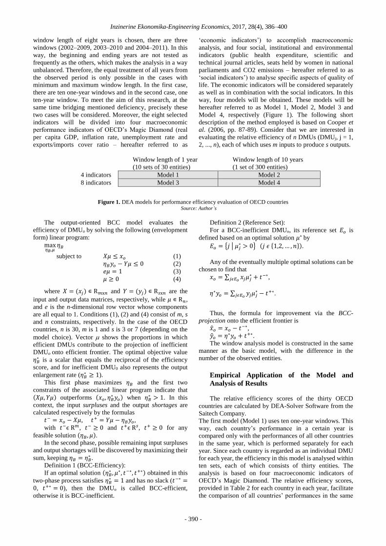
two cases will be considered. Moreover, the eight selected

indicators will be divided into four macroeconomic

performance indicators of OECD’s Magic Diamond (real

per capita GDP, inflation rate, unemployment rate and

exports/imports cover ratio – hereafter referred to as

‘economic indicators’) to accomplish macroeconomic

analysis, and four social, institutional and environmental

indicators (public health expenditure, scientific and

technical journal articles, seats held by women in national

parliaments and CO2 emissions – hereafter referred to as

‘social indicators’) to analyse specific aspects of quality of

life. The economic indicators will be considered separately

as well as in combination with the social indicators. In this

way, four models will be obtained. These models will be

hereafter referred to as Model 1, Model 2, Model 3 and

Model 4, respectively (Figure 1). The following short

description of the method employed is based on Cooper et

al. (2006, pp. 87-89). Consider that we are interested in

evaluating the relative efficiency of n DMUs (DMUj, j = 1,

2, ..., n), each of which uses m inputs to produce s outputs.

Window length of 1 year

(10 sets of 30 entities)

Window length of 10 years

(1 set of 300 entities)

4 indicators Model 1 Model 2

8 indicators Model 3 Model 4

Figure 1. DEA models for performance efficiency evaluation of OECD countries

Source: Author’s

The output-oriented BCC model evaluates the

efficiency of DMUo by solving the following (envelopment

form) linear program:

max𝜂𝐵,𝜇

𝜂𝐵

subject to 𝑋𝜇 ≤ 𝑥𝑜 (1)

𝜂𝐵𝑦𝑜 − 𝑌𝜇 ≤ 0 (2)

𝑒𝜇 = 1 (3)

𝜇 ≥ 0 (4)

where 𝑋 = (𝑥𝑗) ∊ R𝑚x𝑛 and 𝑌 = (𝑦𝑗) ∊ R𝑠x𝑛 are the

input and output data matrices, respectively, while 𝜇 ∊ R𝑛,

and e is the n-dimensional row vector whose components

are all equal to 1. Conditions (1), (2) and (4) consist of m, s

and n constraints, respectively. In the case of the OECD

countries, n is 30, m is 1 and s is 3 or 7 (depending on the

model choice). Vector shows the proportions in which

efficient DMUs contribute to the projection of inefficient

DMUo onto efficient frontier. The optimal objective value

𝜂𝐵∗ is a scalar that equals the reciprocal of the efficiency

score, and for inefficient DMU0 also represents the output

enlargement rate (𝜂𝐵∗ ≥ 1).

This first phase maximizes 𝜂𝐵 and the first two

constraints of the associated linear program indicate that

(𝑋𝜇, 𝑌𝜇) outperforms (𝑥𝑜, 𝜂𝐵∗ 𝑦𝑜) when 𝜂𝐵

∗ > 1. In this

context, the input surpluses and the output shortages are

calculated respectively by the formulas

𝑡− = 𝑥𝑜 − 𝑋𝜇, 𝑡+ = 𝑌𝜇 − 𝜂𝐵𝑦𝑜,

with 𝑡−ϵ R𝑚, 𝑡− ≥ 0 and 𝑡+ϵ R𝑠, 𝑡+ ≥ 0 for any

feasible solution (𝜂𝐵, 𝜇).

In the second phase, possible remaining input surpluses

and output shortages will be discovered by maximizing their

sum, keeping 𝜂𝐵 = 𝜂𝐵∗ .

Definition 1 (BCC-Efficiency):

If an optimal solution (𝜂𝐵∗ , 𝜇∗, 𝑡−∗, 𝑡+∗) obtained in this

two-phase process satisfies 𝜂𝐵∗ = 1 and has no slack (𝑡−∗ =

0, 𝑡+∗ = 0), then the DMUo is called BCC-efficient,

otherwise it is BCC-inefficient.

Definition 2 (Reference Set):

For a BCC-inefficient DMUo, its reference set 𝐸𝑜 is

defined based on an optimal solution 𝜇∗ by

𝐸𝑜 = {𝑗 | 𝜇𝑗∗ > 0} (𝑗 𝜖 {1,2, … , 𝑛}).

Any of the eventually multiple optimal solutions can be

chosen to find that

𝑥𝑜 = ∑ 𝑥𝑗𝜇𝑗∗ + 𝑡−∗

𝑗𝜖𝐸𝑜,

𝜂∗𝑦𝑜 = ∑ 𝑦𝑗𝜇𝑗∗ − 𝑡+∗

𝑗𝜖𝐸𝑜.

Thus, the formula for improvement via the BCC-

projection onto the efficient frontier is

�̂�𝑜 = 𝑥𝑜 − 𝑡−∗,

�̂�𝑜 = 𝜂∗𝑦𝑜 + 𝑡+∗.

The window analysis model is constructed in the same

manner as the basic model, with the difference in the

number of the observed entities.

Empirical Application of the Model and

Analysis of Results

The relative efficiency scores of the thirty OECD

countries are calculated by DEA-Solver Software from the

Saitech Company.

The first model (Model 1) uses ten one-year windows. This

way, each country’s performance in a certain year is

compared only with the performances of all other countries

in the same year, which is performed separately for each

year. Since each country is regarded as an individual DMU

for each year, the efficiency in this model is analysed within

ten sets, each of which consists of thirty entities. The

analysis is based on four macroeconomic indicators of

OECD’s Magic Diamond. The relative efficiency scores,

provided in Table 2 for each country in each year, facilitate

the comparison of all countries’ performances in the same


- 391 -

year as well as the comparison of one country’s efficiency

scores in all years. The highest average efficiency score

(0.849) was achieved in 2011, and the lowest (0.756) in

2002. At the same time, the number of efficient countries

was highest (7) for the years 2006 and 2010, and lowest (2)

for the year 2009. The only consistently efficient countries

were Luxembourg and Norway, while as many as 20

countries showed persistent inefficiency. While some

countries remained consistently low (e.g. Greece and

Turkey), a few fluctuated between high and low efficiency

rating and vice versa (e.g. Poland and Mexico). Except for

the final year of study, Greece was a consistently least

efficient country with the average efficiency score of

0.509521. The average efficiency score (for all countries

over the entire period) of 0.808942 indicates that on average

the countries had 19.1 % ((1 – 0.808942)*100) inefficiency.

The standard deviations are obviously much smaller

when observing the same country in different years than

when observing various countries in the same year. This

gives evidence of rather balanced performance over time on

country level but significant disparities among countries.

These disparities are specifically confirmed by significant

differences between minimum and maximum (1) efficiency

scores. Table 2

Efficiency Scores – Model 1 (4 Indicators, 10 Windows)

Country Year Average

per

country

Std.

dev. 2002 2003 2004 2005 2006 2007 2008 2009 2010 2011

Australia 0.676 0.675 0.715 0.742 0.708 0.639 0.690 0.715 0.820 0.738 0.711924 0.049

Austria 0.799 0.905 0.857 0.839 0.859 0.789 0.904 0.763 0.960 0.894 0.856894 0.061

Belgium 0.733 0.766 0.817 0.829 0.825 0.773 0.785 0.736 0.783 0.818 0.786417 0.035

Canada 0.756 0.757 0.831 0.847 0.829 0.736 0.781 0.676 0.710 0.744 0.766741 0.056

Czech Republic 0.657 0.721 0.726 0.884 0.839 0.717 0.835 0.762 0.903 0.953 0.799748 0.097

Denmark 0.805 0.858 0.878 0.900 0.979 0.762 0.878 0.784 0.857 0.949 0.864881 0.069

Finland 0.875 0.937 0.951 0.914 0.932 0.789 0.824 0.753 0.824 0.779 0.857818 0.073

France 0.718 0.743 0.790 0.782 0.768 0.679 0.726 0.673 0.727 0.775 0.738240 0.041

Germany 0.781 0.830 0.914 0.962 0.976 0.891 0.936 0.818 0.896 0.944 0.894754 0.066

Greece 0.450 0.437 0.522 0.565 0.498 0.444 0.476 0.470 0.562 0.672 0.509521 0.073

Hungary 0.658 0.683 0.682 0.752 0.695 0.663 0.680 0.927 0.926 0.867 0.753363 0.110

Iceland 0.834 1 1 1 1 1 0.883 0.870 0.890 0.916 0.939301 0.067

Ireland 0.860 0.900 0.943 0.964 0.928 0.897 1 0.832 1 0.987 0.931026 0.059

Italy 0.699 0.694 0.769 0.788 0.767 0.711 0.750 0.693 0.744 0.782 0.739655 0.037

Japan 0.771 1 1 1 1 1 1 0.735 1 1 0.950618 0.104

Korea 0.837 0.960 0.989 1 1 0.834 0.871 0.889 1 1 0.938038 0.072

Luxembourg 1 1 1 1 1 1 1 1 1 1 1 0

Mexico 0.897 1 0.912 0.899 0.996 0.722 0.773 0.675 0.727 0.693 0.829298 0.125

Netherlands 1 1 0.922 0.928 0.939 0.858 1 0.941 0.963 0.988 0.953927 0.046

New Zealand 0.744 0.829 0.907 0.914 0.869 0.695 0.804 0.776 0.802 0.857 0.819603 0.070

Norway 1 1 1 1 1 1 1 1 1 1 1 0

Poland 0.604 0.696 0.660 0.752 1 0.896 0.986 0.959 1 0.743 0.829735 0.154

Portugal 0.587 0.613 0.616 0.573 0.581 0.558 0.600 0.567 0.627 0.808 0.612971 0.072

Slovak Republic 0.601 0.659 0.653 0.733 0.675 0.775 0.736 0.696 0.748 0.816 0.709215 0.064

Spain 0.628 0.623 0.624 0.610 0.585 0.560 0.647 0.679 0.741 0.877 0.657443 0.092

Sweden 0.795 0.844 0.975 0.986 0.962 0.817 0.862 0.818 0.889 0.931 0.887988 0.071

Switzerland 1 0.989 1 1 1 0.894 1 0.834 1 1 0.971761 0.059

Turkey 0.722 0.651 0.611 0.573 0.510 0.560 0.534 0.680 0.566 0.508 0.591452 0.073

United Kingdom 0.644 0.756 0.790 0.788 0.728 0.632 0.693 0.653 0.690 0.770 0.714365 0.060

United States 0.559 0.629 0.669 0.673 0.803 0.606 0.670 0.601 0.646 0.660 0.651568 0.065

Average per year 0.756 0.805 0.824 0.840 0.842 0.763 0.811 0.766 0.833 0.849 0.808942 0.067

Std. dev. 0.140 0.153 0.146 0.141 0.159 0.147 0.148 0.127 0.139 0.126 0.128413 0.031

Minimum score 0.450 0.437 0.522 0.565 0.498 0.444 0.476 0.470 0.562 0.508 0.509521 0

No. (%) of efficient countries

4 13 %

6 20 %

5 17 %

6 20 %

7 23 %

4 13 %

6 20 %

2 7 %

7 23 %

5 17 %

2 7 %

Source: Author’s calculations based on data from the World Bank

Because the DEA window models offer valuable

information on relative efficiency trends, their relevance is

beyond doubt. However, these models do not provide

indispensable information on inefficiency sources and

proposed improvements. Getting this information involves

running the basic BCC model ten times – once for each

year’s data for all thirty observed countries. The efficiency

levels for these ten analyses are identical to those shown in

Table 2. The input excesses and output shortfalls, i.e. the

differences between empirical and projected values (or vice

versa) in each input and output, were calculated taking into

account executed scaling of original data for the undesirable

output. They were then averaged per country and are

expressed as percentages of their respective initial values in

Table 3. They represent needed improvements that can be

achieved using the previously explained two-phase

procedure. For example, the mean efficiency score in 2011

was 0.849, implying that on average the countries were 15.1

% inefficient. This entails that, on average, all output levels

should be increased by 17.8 %, without influencing the

initial input levels, to remove radial inefficiency (the first

phase). (1/0.849 – 1)*100 (as explained earlier, the

reciprocal of the efficiency result is the optimal objective

value for the output-oriented model). In the same year,

however, the major output shortfall was in real per capita

GDP, with the average required an increase of 147.4 %. This


- 392 -

implies that the efficiency cannot be achieved only by

increasing all outputs proportionally, but the countries

should further augment output amounts and thus remove

remaining inefficiencies (the second phase). It is intuitively

understandable that largely demanded changes in input and

output quantities indicate cross country divergence. The

numbers in Table 3, therefore, confirm deep development

disparities among OECD countries. Throughout the entire

period, real per capita GDP had the strongest impact on the

efficiency. The only exception was the year 2009, in which

the inflation rate took the lead in influencing the efficiency.

On the other side, the efficiency was least affected by the

inflation rate, with the exceptions of the years 2002 and

2009 in which this was by the ratio of exports to imports.

These two deviations can be explained by following

reasons. 2002 is the year in which the highest standard

deviation in inflation rates, as well as the greatest difference

between their maximum and minimum values, was

observed. At the same time, the two lowest values for the

inflation rate were recorded in 2009. Table 3

Sources of Inefficiency – Model 1 (4 Indicators, 10 Windows)

V a r i a b l e Input and output improvements (%)

2002 2003 2004 2005 2006 2007 2008 2009 2010 2011

Input Inflation

rate -138.7 -8.1 -4.6 0 -0.2 -9.0 -0.8 -382.5 -1.7 -0.8

Outputs

Desirable

Real per capita

GDP 211.5 144.6 173.0 123.6 79.1 178.3 147.6 191.9 64.4 147.4

Exports/imports

cover ratio 37.7 30.0 26.3 23.9 26.1 38.6 31.3 35.6 24.4 21.4

Undesirable Unemployment

rate -48.0 -40.6 -41.2 -39.8 -32.4 -54.7 -38.9 -58.7 -24.7 -54.0


Both of these situations result with the efficient frontier

that is, considering this variable, more distant from

inefficient countries, and is therefore more difficult to attain.

The fact that the average required reduction in the inflation

rate in both cases surpasses 100% means that the majority

of inefficient countries need to reduce the rate of inflation to

negative levels. Since the effect of negative inflation rates is

questionable, and is not the subject of this paper, we do not

add further comments here. These results reveal two

interesting facts about the inflation rate. There are many

factors that affect inflation but are not the subject of this

research. Firstly, it is the only indicator both among the most

and the least influential indicators. Secondly, it is the only

indicator that does not need to be improved in one year

(2005) of the observed period. This is the consequence of

the significant cross-sample dispersion of inflation rates,

which is confirmed by the coefficient of variation that has

by far the highest value (117.9 %) among all the indicators

used to assess the relative efficiency of the OECD countries

(see Table 1).

Since, in this model, all years were considered

separately, the best efficiency result of a given country in a

particular year does not necessarily mean its highest

performance during the entire examined period. It means

only that its performance compared with other countries for

that given year was better than its performance compared

with other countries in the remaining years. Accordingly,

this model is not suitable for direct comparison across

calendar years for each country since the comparison basis

is different for each year. Consequently, it seems

meaningful to extend the comparison to include all countries

in all years, which leads to the second model (Model 2). In

this model, the efficiency evaluation is based on the same

four indicators, but one ten-year window is used. This way,

each country’s performance in each year is compared with

the performances of all other countries in all years. The

efficiency in this model is therefore analysed within one set

of 300 entities. This makes the essential difference between

this and the previous model. The relative efficiency results

of the Model 2 throughout the entire period are presented in

Table 4. As evident, none of the countries has been able to

accomplish continuous efficiency. Out of 300 observed

entities, only eight were relatively efficient. Norway was

efficient in five years, Luxembourg in two years and Iceland

in one year, while the rest of 27 countries showed no

efficiency. No country has shown continuous efficiency

growth, while Finland was the only country with continuous

efficiency decline. The number of efficient countries was

highest (3) for the year 2007, while in the years 2003, 2004,

2005, 2010 and 2011 no country was efficient. The highest

average efficiency score (0.719) was achieved in 2002, and

the lowest (0.688) in 2011. It should be emphasized this is

an entirely opposite result from that of the previous model.

The reason for this turn may be attributed to the different

window length as explained earlier.

The lowest of 300 efficiency scores (0.404) was

obtained by Greece in 2003. Like the previous model, the

lowest average efficiency score was recorded by Greece

(0.446643), while the highest two were achieved by Norway

(0.976003) and Luxembourg (0.960589). These numbers

again testify to the differences among OECD members,

which are here even deeper than in the previous model.

Compared to a year earlier, the most significant efficiency

decrease was recorded by Mexico in 2006 (–0.274). At the

same time, the highest efficiency improvement was

achieved by Japan in 2010 (+0.265). Among other countries,

Luxembourg makes an interesting example since it was

efficient throughout the entire period when years were

observed separately, and only in two years when years were

mutually compared. This is because no country was more

efficient than Luxembourg in, for example, 2011, but some

of them, including Luxembourg itself in 2002, 2006, 2007,

2008, 2009 and 2010, were more efficient in some of the

remaining years. Expectedly, as a conclusion, some

similarities but also distinct differences are indicated by the

results generated by Models 1 and 2. The inefficiency


- 393 -

sources in the form of the demanded input and output

improvements averaged over the observed period are given

in Table 5. In this model, the situation regarding the

indicators’ influence on efficiency levels is much clearer

than in the previous model. Thus, the real per capita GDP

again had the greatest impact on inefficiency, but this time

with no exception and even stronger than in the previous

model. The efficiency was again least affected by the

inflation rate, here also without exception. The fact that,

compared to the previous model, the differences among

OECD countries deepened, again is a direct consequence of

different window length. Considerably greater average

impact of outputs rather than of input on the efficiency is

predetermined by selection of the model orientation. The

third model (Model 3), as well as the first one, uses ten one-

year windows but bases the efficiency assessment on the

complete set of eight selected indicators.

Table 4

Efficiency Scores – Model 2 (4 Indicators, 1 Window)

Country

Year Average

per

country

Std. dev. 2002 2003 2004 2005 2006 2007 2008 2009 2010 2011

Australia 0.650 0.587 0.569 0.576 0.599 0.613 0.600 0.642 0.635 0.666 0.613602 0.033

Austria 0.735 0.715 0.703 0.697 0.709 0.720 0.737 0.707 0.718 0.706 0.714756 0.013

Belgium 0.712 0.709 0.702 0.688 0.687 0.688 0.659 0.684 0.670 0.659 0.685785 0.019

Canada 0.738 0.722 0.736 0.725 0.705 0.691 0.680 0.646 0.612 0.623 0.687651 0.047

Czech Republic 0.633 0.643 0.653 0.691 0.692 0.673 0.692 0.698 0.708 0.706 0.678821 0.027

Denmark 0.765 0.778 0.748 0.739 0.737 0.728 0.735 0.732 0.739 0.740 0.744251 0.016

Finland 0.855 0.805 0.789 0.732 0.732 0.730 0.707 0.694 0.687 0.639 0.736954 0.064

France 0.696 0.685 0.673 0.646 0.635 0.622 0.615 0.629 0.615 0.604 0.641829 0.032

Germany 0.761 0.744 0.768 0.764 0.762 0.776 0.767 0.754 0.754 0.741 0.759080 0.011

Greece 0.431 0.404 0.460 0.470 0.433 0.418 0.422 0.430 0.477 0.522 0.446643 0.035

Hungary 0.601 0.595 0.599 0.630 0.623 0.611 0.603 0.840 0.844 0.703 0.664853 0.098

Iceland 0.752 0.774 0.797 0.905 0.822 1 0.842 0.802 0.804 0.795 0.829301 0.073

Ireland 0.791 0.798 0.795 0.764 0.753 0.767 0.773 0.820 0.807 0.796 0.786399 0.021

Italy 0.669 0.663 0.669 0.650 0.634 0.643 0.636 0.638 0.618 0.621 0.643962 0.018

Japan 0.771 0.788 0.790 0.756 0.747 0.759 0.709 0.696 0.740 0.659 0.741578 0.042

Korea 0.754 0.724 0.747 0.738 0.792 0.786 0.773 0.746 0.724 0.759 0.754448 0.024

Luxembourg 1 0.926 0.928 0.934 0.962 1 0.976 0.953 0.966 0.961 0.960589 0.027

Mexico 0.828 0.805 0.671 0.705 0.762 0.722 0.702 0.620 0.623 0.616 0.705405 0.076

Netherlands 0.932 0.766 0.756 0.756 0.763 0.801 0.894 0.791 0.755 0.757 0.797238 0.064

New Zealand 0.731 0.701 0.681 0.674 0.677 0.681 0.669 0.708 0.702 0.691 0.691604 0.019

Norway 1 0.960 0.951 0.983 1 1 1 1 0.923 0.943 0.976003 0.029

Poland 0.584 0.614 0.598 0.633 0.905 0.837 0.853 0.869 0.914 0.619 0.742479 0.142

Portugal 0.517 0.520 0.505 0.483 0.507 0.522 0.500 0.526 0.530 0.593 0.520316 0.029

Slovak Republic 0.572 0.618 0.611 0.614 0.620 0.651 0.628 0.658 0.651 0.650 0.627305 0.026

Spain 0.598 0.591 0.560 0.535 0.521 0.525 0.545 0.634 0.633 0.659 0.580079 0.050

Sweden 0.773 0.774 0.805 0.785 0.779 0.760 0.742 0.751 0.750 0.733 0.765001 0.022

Switzerland 0.930 0.780 0.810 0.791 0.806 0.838 0.838 0.805 0.831 0.815 0.824256 0.042

Turkey 0.662 0.594 0.558 0.542 0.510 0.513 0.523 0.609 0.503 0.457 0.546940 0.060

United Kingdom 0.594 0.602 0.601 0.603 0.602 0.604 0.600 0.601 0.595 0.622 0.602402 0.008

United States 0.530 0.524 0.539 0.559 0.582 0.585 0.556 0.577 0.574 0.574 0.559991 0.022

Average per year 0.719 0.697 0.692 0.692 0.702 0.709 0.699 0.709 0.703 0.688 0.700984 0.040

Std. dev. 0.139 0.120 0.118 0.122 0.130 0.140 0.135 0.120 0.121 0.108 0.116813 0.029

Minimum score 0.431 0.404 0.460 0.470 0.433 0.418 0.422 0.430 0.477 0.457 0.446643 0.008

Maximum score 1 0.960 0.951 0.983 1 1 1 1 0.966 0.961 0.976003 0.142

No. (%) of efficient

countries

2

7 %

0

0 %

0

0 %

0

0 %

1

3 %

3

10 %

1

3 %

1

3 %

0

0 %

0

0 %

0

0 %


The number of indicators makes the only difference

between two models, thus turning the Model 3 into a kind

of the Model 1 extension.

Table 5

Sources of Inefficiency – Model 2 (4 Indicators, 1 Window)


2002 2003 2004 2005 2006 2007 2008 2009 2010 2011

Input Inflation rate -5.3 -3.4 -4.3 -4.4 -7.8 -2.8 -7.7 -0.4 -0.8 -1.6

Ou

tp

uts

Desirable Real per capita GDP 219.3 213.7 203.7 191.8 181.3 172.8 172.6 180.1 172.3 168.6

Exports/imports cover ratio 44.4 48.1 48.7 49.4 49.2 46.8 48.4 45.2 46.4 48.9

Undesirable Unemployment rate -50.3 -51.0 -52.1 -50.4 -46.9 -42.7 -43.3 -53.8 -56.2 -56.2



- 394 -

Table 6 presents the relative efficiency scores of the

Model 3. Although the comparisons between the results of

the models with the same set of indicators and the different

window length are interesting and bring valuable

conclusions for this research, it is critical to compare the

models with four indicators to those with eight indicators.

This is meaningful if based on the same length windows.

The reason for such a comparison lies in the fact that some

countries which, according to macroeconomic indicators,

belong among the most developed countries, often have

serious problems related to various other domains such as

healthcare, environment, and others.

The best average efficiency result (0.962) was

accomplished in 2010, and the worst (0.928) in 2002. The

average total efficiency score of 0.941865 is evidently much

higher than that in the Model 1 (0.808942). This can be

explained by the fact that the major economies failed to

perform so well on some of the social aspects relative to the

countries with a poorer economic performance. A country

example for each of the social indicators is given as follows.

Luxembourg has the highest CO2 emissions per capita of

all OECD countries. The share of public health expenditure

is particularly low in Switzerland compared to the great

majority of OECD countries. Table 6

Efficiency Scores – Model 3 (8 Indicators, 10 Windows)

Country

Year Average

per country

Std.

dev. 2002 2003 2004 2005 2006 2007 2008 2009 2010 2011

Australia 0.813 0.828 0.858 0.880 0.873 0.891 0.885 0.883 0.896 0.891 0.869835 0.028

Austria 0.928 0.958 0.926 0.920 0.929 0.899 0.942 0.903 0.987 0.949 0.934099 0.026

Belgium 0.869 0.888 0.913 0.919 0.905 0.907 0.918 0.903 0.917 0.896 0.903527 0.016

Canada 0.841 0.847 0.859 0.869 0.869 0.869 0.878 0.867 0.857 0.831 0.858653 0.015

Czech Republic 1 1 1 1 1 0.998 0.966 0.968 1 0.982 0.991494 0.014

Denmark 1 1 1 1 1 1 1 1 1 1 1 0

Finland 1 1 0.973 0.929 1 0.946 0.946 0.942 1 0.960 0.969503 0.029

France 1 0.967 0.959 0.955 0.952 0.952 0.969 1 0.976 0.989 0.971978 0.019

Germany 0.927 0.935 0.934 0.973 1 0.984 1 0.906 0.955 0.953 0.956710 0.032

Greece 0.718 0.718 0.718 0.728 0.750 0.729 0.722 0.818 0.820 0.807 0.752809 0.044

Hungary 0.928 0.913 0.900 0.898 0.898 0.881 0.889 1 1 0.955 0.926239 0.044

Iceland 1 1 1 1 1 1 1 1 1 1 1 0

Ireland 0.893 0.918 0.951 0.968 0.964 0.974 1 1 1 0.987 0.965549 0.036

Italy 0.875 0.878 0.899 0.910 0.915 0.917 0.924 0.915 0.938 0.884 0.905541 0.021

Japan 0.969 1 1 1 1 1 1 0.958 1 1 0.992749 0.016

Korea 0.865 0.960 0.989 1 1 0.848 0.889 0.917 1 1 0.946837 0.062

Luxembourg 1 1 1 1 1 1 1 1 1 1 1 0

Mexico 1 1 1 1 1 1 1 1 1 1 1 0

Netherlands 1 1 1 1 1 1 1 1 1 1 1 0

New Zealand 0.927 0.941 0.964 0.977 1 0.982 0.990 0.979 0.989 0.973 0.972223 0.023

Norway 1 1 1 1 1 1 1 1 1 1 1 0

Poland 0.854 0.861 0.827 0.837 1 0.934 0.999 0.983 1 0.825 0.912086 0.078

Portugal 0.915 0.913 0.907 0.879 0.898 0.887 1 0.956 1 1 0.935440 0.049

Slovak Republic 1 1 0.892 0.899 0.832 0.929 0.836 0.949 0.862 0.865 0.906385 0.062

Spain 0.852 0.852 0.872 0.875 0.878 0.877 0.908 0.917 1 1 0.903013 0.055

Sweden 1 1 1 1 1 1 1 1 1 1 1 0

Switzerland 1 1 1 1 1 1 1 1 1 1 1 0

Turkey 1 1 1 1 1 1 1 1 1 1 1 0

United Kingdom 0.947 0.955 0.972 0.959 0.967 0.958 0.965 0.978 0.987 0.974 0.966348 0.012

United States 0.727 0.733 0.746 0.751 0.803 0.694 0.692 0.669 0.671 0.663 0.714929 0.045

Average per year 0.928 0.935 0.935 0.938 0.948 0.935 0.944 0.947 0.962 0.946 0.941865 0.024

Std. dev. 0.083 0.080 0.076 0.074 0.070 0.079 0.081 0.072 0.075 0.081 0.070860 0.022

Minimum score 0.718 0.718 0.718 0.728 0.750 0.694 0.692 0.669 0.671 0.663 0.714929 0


countries

13

43 %

13

43 %

11

37 %

12

40 %

16

53 %

10

33 %

13

43 %

12

40 %

18

60 %

13

43 %

9

30 %


Japan has comparatively low output of scientific and

technical journal articles on a per capita basis. Ireland

performs very poorly compared to the percentage of women

in other national parliaments. The highest number of

efficient countries (18) corresponds to 2010, while the

lowest number (10) was shown in 2007. Regarding

inefficient countries, only eight out of thirty countries have

been persistently inefficient. At the same time, nine

countries were efficient in all analysed years: Denmark,

Iceland, Luxembourg, Mexico, Netherlands, Norway,

Sweden, Switzerland and Turkey. While, according to the

Model 1 efficiency scores, eight out of these nine countries

performed above-average, Turkey scored well below the

benchmark. This dramatic efficiency change is attributable

solely to the fact that Turkey had the lowest per capita CO2

emissions during the first eight years of the period under

investigation. There is no country whose efficiency

deteriorated compared to the Model 1 and, as expected

based on the previously mentioned, most significant shift in

average efficiency score (+0.408548) was accomplished by

Turkey. For the opposite reason, the United States became

on average the least efficient country (0.714929), with the

lowest efficiency scores in the last five consecutive years.

This could be interpreted as opposed to the fact that the

United States is widely considered one of the strongest

economies in the world. However, the discordance arises


- 395 -

mainly from the selection of indicators. Namely, on one of

the four economic indicators, and on even three of the four

social indicators, the United States performs significantly

worse than average. The mean values across the observed

period for each of these indicators are as follows:

exports/imports cover ratio – US 71.1/OECD 103.0, CO2

emissions – US 18.7/OECD 9.4, public health expenditure

– US 45.5/OECD 72.9, seats held by woman in national

parliaments – US 15.9/OECD 24.6.

Based on much higher minimum efficiency scores and

on much smaller standard deviations within each year in the

Model 3 than in the Model 1, it is concluded that disparities

among countries are much more pronounced when the

countries are compared based on solely economic indicators

than when they are compared based on the combination of

economic and social indicators. The causes of such outcome

are explained on the example of Turkey and the United

States in the preceding paragraph.

The inefficiency sources and proposed improvements,

calculated in the same manner as in the previous models, are

presented in Table 7. These values differ significantly from

the ones obtained with Models 1 and 2. Thus, in the Model

3, real per capita GDP had the strongest impact on efficiency

only in three years (2007, 2008 and 2011), the inflation rate

in one year (2009) and the seats held by women in national

parliaments in the remaining six years. On a general level,

the requested input and output improvements are not nearly

as large as they were in the previous two models, which

testify to smoothed differences among the OECD countries

when they are viewed in terms of the economic and social

indicators combination. During the entire period, it is

evident that public health expenditure and inflation rate

alternate as indicators are least significantly affecting

efficiency.

Table 7

Sources of Inefficiency – Model 3 (8 Indicators, 10 Windows)


2002 2003 2004 2005 2006 2007 2008 2009 2010 2011

Input Inflation

rate -22.7 -8.2 -10.6 -15.8 -8.8 -9.2 -1.7 -60.6 -3.3 -17.5

Outputs

Desirable

Real per capita

GDP 48.3 44.1 48.3 49.0 27.2 75.1 60.3 53.1 19.8 54.9

Exports/imports

cover ratio 15.0 14.1 14.2 14.1 13.1 16.8 12.5 13.6 8.2 9.0

Scientific and technical

journal articles 40.6 42.4 45.1 47.0 33.9 47.0 33.1 25.7 18.1 38.2

Public health

expenditure 9.8 9.1 10.0 8.6 6.6 9.7 8.5 8.4 4.8 7.1

Seats held by women

in national parliaments 56.9 57.8 50.3 54.3 46.1 48.1 43.9 39.8 24.2 42.9

Undesirable

Unemployment

rate -22.6 -19.7 -20.9 -17.3 -12.1 -29.8 -21.7 -35.9 -13.0 -27.1

CO2

emissions -19.5 -19.0 -22.2 -22.1 -18.4 -22.5 -19.8 -13.0 -13.9 -17.8


The fourth model (Model 4) is the result of the tendency

to simultaneously observe all countries in all years, and

based on all eight indicators. Hence, it is the most

comprehensive model among all four models Table 8

Efficiency Scores – Model 4 (8 Indicators, 1 Window)

Country

Year Average

per

country

Std. dev. 2002 2003 2004 2005 2006 2007 2008 2009 2010 2011

Australia 0.775 0.762 0.770 0.785 0.793 0.829 0.838 0.845 0.865 0.891 0.815328 0.044

Austria 0.881 0.868 0.865 0.869 0.875 0.880 0.894 0.892 0.888 0.892 0.880300 0.011

Belgium 0.856 0.867 0.888 0.891 0.881 0.875 0.892 0.900 0.905 0.894 0.884950 0.015

Canada 0.811 0.816 0.821 0.823 0.816 0.823 0.826 0.840 0.824 0.831 0.823078 0.008

Czech Republic 1 1 0.992 0.982 0.974 0.960 0.939 0.951 0.962 0.963 0.972398 0.021

Denmark 0.979 0.979 0.977 0.979 0.979 0.982 0.993 0.990 0.992 1 0.984908 0.008

Finland 0.906 0.894 0.887 0.882 0.893 0.925 0.929 0.917 0.920 0.959 0.911320 0.023

France 0.939 0.919 0.917 0.916 0.915 0.920 0.920 0.981 0.945 0.975 0.934596 0.025

Germany 0.914 0.906 0.893 0.889 0.888 0.891 0.890 0.895 0.891 0.889 0.894652 0.009

Greece 0.681 0.699 0.690 0.700 0.723 0.706 0.705 0.800 0.793 0.802 0.729878 0.048

Hungary 0.870 0.865 0.854 0.856 0.851 0.840 0.839 1 1 0.929 0.890342 0.063

Iceland 0.972 0.975 0.969 0.981 0.979 1 1 1 1 1 0.987586 0.014

Ireland 0.882 0.896 0.892 0.887 0.880 0.883 0.887 0.980 0.867 0.872 0.892561 0.032

Italy 0.862 0.864 0.877 0.881 0.884 0.889 0.893 0.899 0.905 0.880 0.883437 0.014

Japan 0.941 0.934 0.936 0.945 0.938 0.948 0.950 0.946 0.958 0.961 0.945626 0.009

Korea 0.779 0.769 0.782 0.783 0.809 0.797 0.783 0.778 0.743 0.763 0.778567 0.018

Luxembourg 1 0.968 0.965 0.966 0.976 1 1 0.988 0.995 1 0.985789 0.015

Mexico 1 1 0.992 0.971 0.974 0.957 0.944 1 1 0.983 0.981999 0.020

Netherlands 0.950 0.894 0.865 0.865 0.983 0.989 1 1 1 1 0.954539 0.058


- 396 -

Country

Year Average

per country

Std.

dev. 2002 2003 2004 2005 2006 2007 2008 2009 2010 2011

New Zealand 0.909 0.911 0.930 0.936 0.941 0.966 0.970 0.964 0.964 0.967 0.945849 0.024

Norway 1 0.993 0.991 0.997 1 1 1 1 1 1 0.998060 0.003

Poland 0.826 0.817 0.802 0.814 0.926 0.879 0.893 0.914 0.937 0.819 0.862563 0.052

Portugal 0.852 0.839 0.850 0.838 0.838 0.826 0.891 0.915 0.983 1 0.883159 0.063

Slovak Republic 1 1 0.861 0.864 0.807 0.807 0.808 0.888 0.824 0.848 0.870673 0.073

Spain 0.831 0.833 0.843 0.845 0.851 0.854 0.865 0.912 0.937 0.936 0.870783 0.042

Sweden 0.987 0.991 0.991 0.991 1 1 1 1 0.995 1 0.995557 0.005

Switzerland 1 0.938 0.963 0.931 0.948 1 1 0.971 1 1 0.975117 0.029

Turkey 1 1 1 1 0.943 0.919 0.929 1 0.970 0.972 0.973319 0.032

United Kingdom 0.920 0.918 0.937 0.935 0.941 0.933 0.944 0.962 0.964 0.964 0.941841 0.017

United States 0.591 0.599 0.631 0.658 0.672 0.677 0.661 0.648 0.656 0.663 0.645724 0.029

Average per year 0.897 0.890 0.888 0.889 0.896 0.898 0.903 0.926 0.923 0.922 0.903150 0.027

Std. dev. 0.101 0.096 0.090 0.085 0.082 0.085 0.086 0.081 0.086 0.084 0.083004 0.019

Minimum score 0.591 0.599 0.631 0.658 0.672 0.677 0.661 0.648 0.656 0.663 0.645724 0.003

Maximum score 1 1 1 1 1 1 1 1 1 1 0.998060 0.073


countries

7

23 %

4

13 %

1

3 %

1

3 %

2

7 %

5

17 %

6

20 %

7

23 %

6

20 %

8

27 %

0

0 %


used in this research. In this model, as well as in the second

one, one ten-year window is used and the efficiency is

assessed based on all eight indicators. As well as in the case

of Models 1 and 3, the difference between Models 2 and 4 is

in the number of the observed indicators.

The highest average efficiency result (0.926) was

achieved in 2009, and the lowest (0.888) in 2004. While only

one country was efficient for the years 2004 and 2005, even

eight of them were efficient for the final year of the observed

period. The results produced by this model can be compared

to the results of the previous models by two different criteria

– the same window length (to the results given by the Model

2) and the same set of indicators (to the results obtained by

the Model 3).

As in the case of Models 1 and 3, the average total

efficiency score (0.903150) in the model developed based

on eight indicators (Model 4) is much higher than that

(0.700984) in the model developed based on four indicators

(Model 2). Similar to the Model 2, none of the countries has

been continuously efficient. Unlike in the Model 2, where

only eight out of 300 entities were efficient, in this model,

there were 47 efficient entities. Norway was efficient in

seven years, Iceland, Sweden, Switzerland, and Turkey in

five years, Luxembourg, Mexico and Netherlands in four

years, Czech Republic, Hungary and Slovak Republic in

two years, and Denmark and Portugal in one year, while the

rest of 17 countries showed no efficiency. Also contrary to

the Model 2, there was no year in which no country was

efficient. The worst of 300 efficiency results (0.591) was

registered by the United States in 2002, while in the Model

2 it was Greece in 2003. This confirms the anticipated

conclusion about much less pronounced cross-country

differences after the incorporation of social indicators. The

highest average efficiency scores were recorded by two

Scandinavian countries – Norway (0.998060) and Sweden

(0.995557), while in the Model 2 it was Norway and

Luxembourg with slightly lower efficiency values. As in the

case of the models with the window length of one year, and

for the same reasons, broadening the set of indicators caused

no worsening of the efficiency scores and Turkey achieved

the most noticeable shift in average efficiency score

(+0.426379).

As the comparison of Models 1 and 2, there are certain

resemblances as well as significant dissimilarities between

the results generated by Models 3 and 4. As in the Model 3,

no country has experienced permanent efficiency growth,

and the United States was again on average by far the least

efficient country (0.645724), with the worst efficiency

results in all ten years observed. Contrary to the Model 3, no

country has shown permanent efficiency decline.

To complete the comparison of this model with its

predecessors, it is important to accurately determine which

inputs and outputs are causing inefficiency and to what

extent. The sources of inefficiency, as well as the size of

their impact, are presented in Table 9.

Table 9

Sources of Inefficiency – Model 4 (8 Indicators, 1 Window)


2002 2003 2004 2005 2006 2007 2008 2009 2010 2011

Input Inflation rate -3.6 -3.5 -11.2 -7.8 -13.5 -11.3 -8.9 -4.2 -8.4 -11.4

Ou

tputs

Des

irab

le

Real per capita GDP 60.1 60.5 64.4 65.4 66.3 66.2 64.7 51.3 56.4 58.3

Exports/imports cover ratio 14.2 16.1 17.4 17.9 19.6 17.3 17.7 13.6 14.8 13.8

Scientific and technical journal articles

66.3 80.0 69.1 67.7 53.4 59.3 47.4 30.2 30.2 39.1

Public health expenditure 15.0 15.4 16.1 15.5 14.5 13.9 12.8 9.8 10.2 10.4

Seats held by women in national

parliaments 66.4 67.7 67.5 68.4 64.9 60.9 61.0 48.5 51.6 52.7

Undesirable Unemployment rate -25.1 -28.5 -30.7 -28.2 -26.2 -20.0 -17.9 -29.1 -32.8 -29.8

CO2 emissions -15.6 -17.7 -19.2 -20.0 -19.3 -20.5 -20.0 -17.8 -19.4 -18.9



- 397 -

Even though the efficiency of OECD countries in this

model was measured through the prism of the same eight

economic and social indicators as in the Model 3, the

outcomes of these two models are quite different. Thus, in

the Model 4, the most important role in affecting the

efficiency in the first four years was divided between

scientific and technical journal articles (2003 and 2004) and

seats held by women in national parliaments (2002 and

2005), while during the remaining six years that role was

taken over by real per capita GDP. Interestingly, the first of

these three indicators was not the primary source of

inefficiency in the Model 3 even in one year. Also unlike the

Model 3 where it was the least significant inefficiency

source in six years, public health expenditure had a minimal

impact on efficiency in the Model 4 only in the final year,

while during the entire remaining period this has been the

inflation rate. The model orientation towards outputs

initiates generally stronger role of output rather than input

variables in achieving efficiency. The fact that, in general

terms, the required changes of all seven outputs in this

model outgrew those in the Model 3 can be once more

attributed to the difference between the window lengths

which dictate the number and hence the size of comparison

sets. At the same time, the cross-OECD-country disparities

in the Model 4 were on average significantly diminished

when compared to those in Models 1 and 2, for the earlier

mentioned reason of the addition of social indicators. This

effect, along with the difference in window lengths, explains

the easily observable fact that each of the four models

employed resulted in different relative efficiency scores.

Table 10 summarizes the impact of adding the four

social indicators to the list of four macroeconomic

indicators on the results of the models based on one-year

windows. To simplify reporting, the first and second rank

orders were averaged to provide a unique ranking for each

country. The biggest loser from this turn toward social

factors was Korea. This can be explained by Korea’s worse

than average performance in all four social indicators, which

Table 10

Country Rankings by Average Efficiency Score, Ten One-Year Windows

Country Model 1 Model 3 Change Average

rank order

Australia 24 27 –3 27

Austria 13 20 –7 17

Belgium 18 25 –7 22

Canada 19 28 –9 24

Czech Republic 17 11 +6 14

Denmark 11 1 +10 7

Finland 12 14 –2 12

France 22 13 +9 18

Germany 9 17 –8 12

Greece 30 29 +1 30

Hungary 20 21 –1 21

Iceland 6 1 +5 5

Ireland 8 16 –8 10

Italy 21 24 –3 23

Japan 5 10 –5 8

Korea 7 18 –11 11

Luxembourg 1 1 0 1

Mexico 15 1 +14 9

Netherlands 4 1 +3 4

New Zealand 16 12 +4 14

Norway 1 1 0 1

Poland 14 22 –8 19

Portugal 28 19 +9 24

Slovak Republic 25 23 +2 26

Spain 26 26 0 28

Sweden 10 1 +9 6

Switzerland 3 1 +2 3

Turkey 29 1 +28 16

United Kingdom 23 15 +8 20

United States 27 30 –3 29

Source: Author’s calculations

Table 11

Country Rankings by Average Efficiency Score, One Ten-Year Window


rank order

Australia 24 27 –3 28

Austria 14 22 –8 15

Belgium 18 19 –1 19

Canada 17 26 –9 24

Czech Republic 19 9 +10 13

Denmark 10 5 +5 6

Finland 13 15 –2 13

France 22 14 +8 15


- 398 -


rank order

Germany 8 16 –8 10

Greece 30 29 +1 30

Hungary 20 18 +2 21

Iceland 3 3 0 2

Ireland 6 17 –11 9

Italy 21 20 +1 23

Japan 12 12 0 10

Korea 9 28 –19 19

Luxembourg 2 4 –2 2

Mexico 15 6 +9 8

Netherlands 5 10 –5 6

New Zealand 16 11 +5 12

Norway 1 1 0 1

Poland 11 25 –14 15

Portugal 29 21 +8 27

Slovak Republic 23 24 –1 25

Spain 26 23 +3 26

Sweden 7 2 +5 4

Switzerland 4 7 –3 5

Turkey 28 8 +20 15

United Kingdom 25 13 +12 21

United States 27 30 –3 29

Source: Author’s calculations

is particularly evident in the per capita number of scientific

and technical journal articles. On the other hand, and for the

reasons explained earlier, by far the biggest gainer from this

change in point of view was, as expected, the less

industrialized Turkey. These drastic oscillations in the

rankings once again strongly confirm the influence of the

inclusion of social indicators in evaluating the relative

macroeconomic performance of nations. Table 11 is

analogous to Table 10, but refers to the country rankings in

Models 2 and 4. As in the previous case, the inclusion of

social indicators had most and least favourable influence on

Turkey and Korea respectively. Comparing this impact with

the previous one, it can be noted that its magnitude is

increased in the case of Korea and decreased in the case of

Turkey.

Comparing the average rank orders from Tables 10 and

11 for each country, it can be seen that some countries

perform relatively better according to the models based on

one-year windows, while the others respond better to

models with a ten-year window.

Concluding Remarks

The relative efficiency of the OECD members was

empirically assessed based on the reciprocal performance

comparison of thirty countries, using DEA window analysis.

The analysis included time-series cross-country comparisons

using a ten-year period, thus enabling simultaneous

monitoring of the efficiency dynamics of the countries. By

employing four models with the assumption of variable

returns-to-scale, which differs in the window lengths and the

indicator sets, the countries’ performances were compared

within and between years, integrating economic, social,

institutional and environmental objectives.

The empirical results suggest several important

findings. Firstly, when it comes to the efficiency scores

averaged across all ten years of data collection, Norway was

ranked first regardless of the model used. At the same time,

Greece performed worst according to the models with only

economic indicators, and the United States was ranked last

in the models with the combination of economic and social

indicators. Secondly, based on the amount of inefficiency

for each country, we derived the amount of inefficiency for

the OECD countries as a whole. This amount suggests that

there are definite possibilities of increasing efficiency

levels. The average overall inefficiency hence could be

reduced by 5.8 % to 29.9 %, depending on the model choice.

Thirdly, as a general conclusion, by far the most frequent

major source of inefficiency was GDP, while the inflation

rate was most commonly the least significant inefficiency

source. Main study result is in accordance with most growth

econometrics papers (Durlauf et al., 2005) identifying

starting GDP level as the most important economic growth

determinant. The same result is validated in this study.

The findings of this study, based on cross-country

comparisons, should be of interest to analysts and should

assist policymakers in each country in identifying the

strengths and weaknesses of its socio-economic performance,

and thus in designing a targeted socio-economic policy. They

give an insight into the level and dynamics of relative

efficiency and result in guidelines for creating new or

recreating existing socio-economic conditions in OECD

countries. To make this insight more comprehensive, the

analysis through the proposed models should be expanded

to include more countries worldwide, to span over a longer

period and to incorporate more indicators that would

address many additional aspects of socio-economic

development. These possibilities remain open for future

investigation.


- 399 -

Acknowledgment

This work has been fully supported by the Croatian Science Foundation under the project number 9481 Modelling Economic

Growth - Advanced Sequencing and Forecasting Algorithm. Any opinions, findings, and conclusions or recommendations

expressed in this material are those of the author(s) and do not necessarily reflect the views of Croatian Science Foundation.

Comments from the Editor and two anonymous reviewers are gratefully acknowledged.

References

Afonso, A., & St. Aubyn, M. (2013). Public and private inputs in aggregate production and growth – a cross-country

efficiency approach. Applied Economics, 45(32), 4487–4502. https://doi.org/10.1080/00036846.2013.791018

Arcelus, F. J., & Arocena, P. (2000). Convergence and productive efficiency in fourteen OECD countries: a non-parametric

frontier approach. International Journal of Production Economics, 66(2), 105–117. https://doi.org/10. 1016/S0925-

5273(99)00116-4

Arcelus, F. J., & Arocena, P. (2005). Productivity differences across OECD countries in the presence of environmental

constraints. Journal of the Operational Research Society, 56(12), 1352–1362. https://doi.org/10.1057/palgrave.

jors.2601942

Banker, R. D., Charnes, A., & Cooper, W. W. (1984). Some Models for Estimating Technical and Scale Inefficiencies in

Data Envelopment Analysis. Management Science, 30(9), 1078–1092. https://doi.org/10.1287/mnsc.30.9.1078

Barla, P., & Perelman, S. (2005). Sulphur emissions and productivity growth in industrialised countries. Annals of Public

& Cooperative Economics, 76(2), 275–300. https://doi.org/10.1111/j.1370-4788.2005.00279.x

Blazejowski, M., Gazda, J., & Kwiatkowski, J. (2016). Bayesian Model Averaging in the Studies on Economic Growth in

the EU Regions-Application of the gretl BMA package. Economics & Sociology, 9(4), 168.

Brockett, P. L., Golany, B., & Li, S. (1999). Analysis of Intertemporal Efficiency Trends Using Rank Statistics with an

Application Evaluating the Macro Economic Performance of OECD Nations. Journal of Productivity Analysis, 11(2),

169–182. https://doi.org/10.1023/A:1007788117626

Calmfors, L., & Driffill, J. (1988). Bargaining structure, corporatism and macroeconomic performance, Economic policy,

3(6), 13–61. https://doi.org/10.2307/1344503

Camarero, M., Castillo, J., Picazo-Tadeo, A. J., & Tamarit, C. (2013). Eco-efficiency and convergence in OECD countries.

Environmental and Resource Economics, 55(1), 87–106. https://doi.org/10.1007/s10640-012-9616-9

Camarero, M., Picazo-Tadeo, A.J., & Tamarit, C. (2008). Is the environmental performance of industrialized countries

converging? A 'SURE' approach to testing for convergence. Ecological Economics, 66(4), 653–661. https://doi.org/10.

1016/j.ecolecon.2007.10.024

Charnes, A., Cooper, W. W., & Rhodes, E. (1978). Measuring the Efficiency of Decision Making Units. European Journal

of Operational Research, 2(6), 429–444. https://doi.org/10.1016/0377-2217(78)90138-81

Cherchye, L. (2001), Using data envelopment analysis to assess macroeconomic policy performance. Applied Economics,

33(3), 407–416. https://doi.org/10.1080/00036840122353

Cooper, W. W., Seiford, L. M., & Tone, K. (2006). Introduction to Data Envelopment Analysis and Its Uses: With DEA-

Solver Software and References, Springer, New York.

Durlauf, S. N., Johnson, P. A., and Temple, J. R. W. (2005). Growth econometrics. In P. Aghion and S. N. Durlauf (eds.)

Handbook of Economic Growth, Volume 1A, North-Holland: Amsterdam, 2005, pp. 555–677. https://doi.org/10.1016

/S1574-0684(05)01008-7

Emrouznejad, A. (2003). An alternative DEA measure: a case of OECD countries. Applied Economics Letters, 10(12), 779–

782. https://doi.org/10.1080/1350485032000126703

Fare, R., Grosskopf, S., & Hernandez-Sancho, F. (2004). Environmental performance: an index number approach. Resource

and Energy economics, 26(4), 343–352. https://doi.org/10.1016/j.reseneeco.2003.10.003

Fare, R., Grosskopf, S., Norris, M., & Zhang, Z. (1994). Productivity Growth, Technical Progress, and Efficiency Change

in Industrialized Countries. American Economic Review, 84(1), 66–83.

Fidrmuc, J., & Kostagianni, S. (2015). Impact of Imf Assistance on Economic Growth Revisited 1. Economics & Sociology,

8(3), 32. https://doi.org/10.14254/2071-789X.2015/8-3/2

Halkos, G. E., & Tzeremes, N. G. (2009). Exploring the existence of Kuznets curve in countries' environmental efficiency

using DEA window analysis. Ecological Economics, 68(7), 2168–2176. https://doi.org/10.1016/j.ecolecon. 2009.02.018

Jakubowska, A., Horvathova, Z. (2016), Economic Growth and Health: A Comparative Study of the EU Countries. Economics

and Sociology, 9(3), 158–168.

https://doi.org/10.1080/00036846.2013.791018

https://doi.org/10.%201016/S0925-5273(99)00116-4

https://doi.org/10.%201016/S0925-5273(99)00116-4

https://doi.org/10.1057/palgrave.%20jors.2601942

https://doi.org/10.1057/palgrave.%20jors.2601942

https://doi.org/10.1287/mnsc.30.9.1078

https://doi.org/10.1111/j.1370-4788.2005.00279.x

https://doi.org/10.1023/A:1007788117626

https://doi.org/10.2307/1344503

https://doi.org/10.1007/s10640-012-9616-9

https://doi.org/10.%201016/j.ecolecon.2007.10.024

https://doi.org/10.%201016/j.ecolecon.2007.10.024

https://doi.org/10.1016/0377-2217(78)90138-8

https://doi.org/10.1080/00036840122353

https://doi.org/10.1016%20/S1574-0684(05)01008-7

https://doi.org/10.1016%20/S1574-0684(05)01008-7

https://doi.org/10.1080/1350485032000126703

https://doi.org/10.1016/j.reseneeco.2003.10.003

https://doi.org/10.14254/2071-789X.2015/8-3/2

https://doi.org/10.1016/j.ecolecon.%202009.02.018


- 400 -

Liu, J. S., Lu, L. Y., Lu, W. M., & Lin, B. J. (2013). Data envelopment analysis 1978–2010: A citation-based literature survey.

Omega, 41(1), 3–15. https://doi.org/10.1016/j.omega.2010.12.006

Lovell, C. A. K., Pastor, J. T., &Turner, J. A. (1995). Measuring macroeconomic performance in the OECD: A comparison of

European and non-European countries. European Journal of Operational Research, 87(3), 507–518.

https://doi.org/10.1016/0377-2217(95)00226-X

Lu, C. C., Chiu, Y. H., Shyu, M. K., & Lee, J. H. (2013). Measuring CO2 emission efficiency in OECD countries: application

of the hybrid efficiency model. Economic Modelling, 32, 130–135. https://doi.org/10. 1016/j.econmod. 2013.01.047

Makridou, G., Andriosopoulos, K., Doumpos, M., & Zopounidis, C. (2016). Measuring the efficiency of energy-intensive

industries across European countries. Energy Policy, 88, 573-583. https://doi.org/10.1016/j. enpol.2015.06.042

Mardani, A., Jusoh, A., Khalil MD Nor, Khalifah, Z., Zakwan, N., Valipour, A. (2015). Multiple criteria decision-making

techniques and their applications – a review of the literature from 2000 to 2014. Economic Research-Ekonomska

Istrazivanja, 28(1), 516-571. https://doi.org/10.1080/1331677X.2015.1075139

Maudos, J., Pastor, J. M., & Serrano, L. (1999). Total factor productivity measurement and human capital in OECD countries.

Economics letters, 63(1), 39–44. https://doi.org/10.1016/S0165-1765(98)00252-3

McCracken, P. W. (1977). Towards full employment and price stability, OECD, Paris.

Moesen, W. W., & Cherchye, L. (1998). The Macroeconomic Performance of Nations: Measurement and Perception,

Discussion Paper Series DPS 98.22, Centre for Economic Studies, Catholic University of Leuven.

OECD (2001). OECD Science, Technology, and Industry Scoreboard, OECD, Paris.

Okun, A. M. (1970). The political economy of prosperity. Brookings Institute Press.

Rashidi, K., & Saen, R. F. (2015). Measuring eco-efficiency based on green indicators and potentials in energy saving and

undesirable output abatement. Energy Economics, 50, 18–26. https://doi.org/10.1016/j.eneco.2015.04.018

Rashidi, K., Shabani, A., & Saen, R. F. (2015). Using data envelopment analysis for estimating energy saving and undesirable

output abatement: a case study in the Organization for Economic Co-Operation and Development (OECD) countries.

Journal of Cleaner Production, 105, 241–252. https://doi.org/10.1016/j.jclepro.2014.07.083

Simionescu, M. (2013). The use of VARMA models in forecasting macroeconomic indicators. Economics & Sociology, 6(2),

94. https://doi.org/10.14254/2071-789X.2013/6-2/9

Simionescu, M., Dobes, K., Brezina, I., & Gaal, A. (2016). GDP rate in the European Union: simulations based on panel data

models. Journal of International Studies, 9(3), 191–202.

Simsek, N. (2014). Energy efficiency with undesirable output at the economy-wide level: cross-country comparison in OECD

sample. American Journal of Energy Research, 2(1), 9–17. https://doi.org/10.12691/ajer-2-1-2

Sueyoshi, T., Yuan, Y., & Goto, M. (2017). A Literature Study for DEA Applied to Energy and Environment. Energy

Economics, (62), 104–124. https://doi.org/10.1016/j.eneco.2016.11.006

Streimikiene, D., Mikalauskiene, A., & Mikalauskas, I. (2016). Comparative Assessment of Sustainable Energy Development

in the Czech Republic, Lithuania and Slovakia. Journal of Competitiveness, 8 (2), 31–41.

https://doi.org/10.7441/joc.2016.02.03

Woo, C., Chung, Y., Chun, D., Seo, H., & Hong, S. (2015). The static and dynamic environmental efficiency of renewable

energy: A Malmquist index analysis of OECD countries. Renewable and Sustainable Energy Reviews, 47, 367–376.

https://doi.org/10.1016/j.rser.2015.03.070

Zaim, O., & Taskin, F. (2000). Environmental efficiency in carbon dioxide emissions in the OECD: A non-parametric

approach. Journal of Environmental Management, 58(2), 95–107. https://doi.org/10.1006/jema.1999.0312

Zhou, P., & Ang, B. W. (2008). Linear programming models for measuring economy-wide energy efficiency performance.

Energy Policy, 36(8), 2911–2916. https://doi.org/10.1016/j.enpol.2008.03.041

Zhou, P., Ang, B. W., & Poh, K. L. (2006). Slacks-based efficiency measures for modeling environmental performance.

Ecological Economics, 60(1), 111–118. https://doi.org/10.1016/j.ecolecon.2005.12.001

Zhou, P., Poh, K. L., & Ang, B. W. (2007). A non-radial DEA approach to measuring environmental performance. European

Journal of Operational Research, 178(1), 1–9. https://doi.org/10.1016/j.ejor.2006.04.038

Zofio, J. L., & Prieto, A. M. (2001). Environmental efficiency and regulatory standards: The case of CO2 emissions from

OECD industries. Resource and Energy Economics, 23(1), 63–83. https://doi.org/10.1016/S0928-7655(00)00030-0

The article has been reviewed.

Received in July, 2017; accepted in October, 2017.

https://doi.org/10.1016/j.omega.2010.12.006

https://doi.org/10.1016/0377-2217(95)00226-X

https://doi.org/10.%201016/j.econmod.%202013.01.047

https://doi.org/10.1016/j.%20enpol.2015.06.042

https://doi.org/10.1080/1331677X.2015.1075139

https://doi.org/10.1016/S0165-1765(98)00252-3

https://doi.org/10.1016/j.eneco.2015.04.018

https://doi.org/10.1016/j.jclepro.2014.07.083

https://doi.org/10.14254/2071-789X.2013/6-2/9

https://doi.org/10.12691/ajer-2-1-2

https://doi.org/10.1016/j.eneco.2016.11.006

https://doi.org/10.7441/joc.2016.02.03

https://doi.org/10.1016/j.rser.2015.03.070

https://doi.org/10.1006/jema.1999.0312

https://doi.org/10.1016/j.enpol.2008.03.041

https://doi.org/10.1016/j.ecolecon.2005.12.001

https://doi.org/10.1016/j.ejor.2006.04.038

https://doi.org/10.1016/S0928-7655(00)00030-0

Documents

Measuring Sources of Economic ... - Engineering Economics