Measuring Socioeconomic Status (SES) in the NCVS

January 6, 2014

Measuring Socioeconomic Status (SES) in the NCVS: Background, Options, and Recommendations

Report

Prepared for

Bureau of Justice Statistics U.S. Department of Justice

810 7th St NW Washington, DC 20531

Prepared by Marcus Berzofsky, DrPH

Hope Smiley-McDonald, PhD Andrew Moore, MS

Chris Krebs, PhD RTI International

3040 E. Cornwallis Road Research Triangle Park, NC 27709

RTI Project Number 0213170.001.002.001

Measuring Socioeconomic Status (SES) in the NCVS: Background, Options, and Recommendations

Prepared by

Marcus Berzofsky, DrPH Darryl Creel, MS

Andrew Moore, MS Hope Smiley-McDonald, PhD

Chris Krebs, PhD

Any opinions and conclusions expressed herein are those of the author(s) and do not necessarily represent the views of the Bureau of Justice Statistics and the U.S. Department

of Justice.

This document was prepared using Federal funds provided by the U.S. Department of Justice under Cooperative Agreement number 2011-NV-CX-K068. The BJS Project Managers were Lynn Langton, BJS Statistician, and Michael Planty, Victimization Unit Chief.

iii

CONTENTS

Section Page

Introduction .......................................................................................................................1

1 Socioeconomic Status—Importance and Measurement ...................................................2

1.1 Background ..............................................................................................................2

1.2 Use of SES in Crime and Victimization Literature .................................................5

1.3 Measuring SES in Other Federal Surveys .............................................................10

2 Recommendation for Using Measures of Socioeconomic Status in Future Reports From the National Crime Victimization Survey ...............................................12

2.1 Single Measure as a Proxy for SES .......................................................................12

2.1.1 Common Single Measures of SES .............................................................12

2.1.2 Alternative Single Measures for SES ........................................................19

2.1.3 Macro-level Single Measures of SES ........................................................20

2.2 Composite SES Measure for NCVS ......................................................................21

2.2.1 Factors Considered for Composite SES Indexes .......................................21

2.2.2 Considered SES Indexes ............................................................................22

2.2.3 Assessing the Quality of the SES Indexes .................................................29

2.3 Conclusions and Recommendation ........................................................................31

2.4 Operationalizing SES in Future Reports ................................................................34

2.5 How to Use the SES Index When Analyzing Crime Victimization Data ..............35

3 Improving the Measurement of Socioeconomic Status in the National Crime Victimization Survey ......................................................................................................36

References ................................................................................................................................43

A Referenced Tables...........................................................................................................49

LIST OF TABLES

Table Page

2-1. Victimization rates by type of crime and household income, 2010 ..............................13

2-2. Distribution of income among NCVS respondents, 1998–2012 ...................................14

2-3. NCVS income categories (question 12a) ......................................................................15

2-4. 2012 Federal poverty level for the 48 contiguous States and the District of Columbia .......................................................................................................................16

2-5. Comparison of population distribution as a percentage of the Federal poverty level as estimated by the NCVS and the CPS, 2008, 2009, 2010, 2011, and 2012 ...............................................................................................................................16

2-6. Victimization rates by type of crime victimization and percentage of Federal poverty level, 2010 ........................................................................................................17

2-7. Victimization rates by type of crime and education level, 2010 ...................................18

2-8. Distribution of level of education by year, 2004–2012.................................................18

2-9. Victimization rates by type of crime and 6-month employment status, 2010 ..............19

2-10. Victimization rates by type of crime and housing tenure, 2010 ...................................20

2-11. SES index options for NCVS ........................................................................................23

2-12. Unweighted sample size and weighted percent distribution of respondents by SES index options, 2010 ...............................................................................................25

2-13. Correlation matrix between NCVS characteristics considered for an SES index .........25

2-14. Logistic regression of violent and property crime victimization by SES index characteristics ................................................................................................................26

2-15. Victimization rates by type of crime and SES Index 1, 2010 .......................................28

2-16. Correlations among SES index options and index characteristics by split sample ...........................................................................................................................31

2-17. Option for reclassifying SES Index Option 1 into three categories ..............................34

LIST OF FIGURES

Figure Page

2-1. Violent crime victimization rates by SES for three index options, 2010 ......................24

2-2. Property crime victimization rates by SES for three index options, 2010 ....................24

1

INTRODUCTION

The National Crime Victimization Survey (NCVS) is the most important source of

information on criminal victimization in the United States. Each year, data from a nationally

representative sample of about 40,000 households comprising nearly 75,000 persons are obtained

on the frequency, characteristics, and consequences of criminal victimization. The survey

enables the Bureau of Justice Statistics (BJS) to estimate the likelihood of experiencing rape,

sexual assault, robbery, assault, theft, household burglary, and motor vehicle theft victimization

for the population as a whole as well as for segments of the population.

One of BJS’s goals for the NCVS is to continually improve its utility so that

victimization can be better understood as crime and its correlates change over time. Recently,

BJS has been interested in assessing the measurement of variables that have long been associated

with victimization, including factors such as socioeconomic status (SES). The goals of this paper

are to (1) understand how other studies have measured SES and identify variables within the

NCVS that could be used to measure or be proxies for SES, (2) explore options for creating an

SES index that could enhance BJS’s analysis of victimization and its correlates, and (3) assess

how components of a potential SES index are currently measured in the NCVS and consider

ways in which they can be improved.

Section 1 summarizes the literature on how SES has been measured in the scientific

literature and how it relates to crime and victimization. Section 2 summarizes the recommended

approach for creating a measure of SES via an index that includes imputed income data. Finally,

Section 3 recommends changes to the NCVS that would address the current limitations and

allow for better measurement of SES and its components.

2

SECTION 1. SOCIOECONOMIC STATUS—IMPORTANCE AND MEASUREMENT

1.1 Background

Socioeconomic factors are vital determinants of human behavior and functioning across

the lifespan (American Psychological Association [APA], 2007). Most commonly referred to as

socioeconomic status (SES) within the health, social, and criminological literature, the

terminology for socioeconomic factors can vary widely (e.g., “socioeconomic position,” “social

disadvantage,” and “socioeconomic deprivation”). Broadly, the APA describes SES as the social

standing or class of an individual or group, often measured as a combination of education,

income, and occupation (APA, 2007). SES also captures an individual’s or a group’s access to

financial, social, cultural, and human capital resources (APA, 2007; National Center for

Education Statistics, 2012; Shavers, 2007).

As Oakes and Rossi noted in 2003, there is a substantial gap between studies that

evaluate how SES is measured and studies that include SES as a variable of interest, and this

situation has not changed appreciably in the past decade. There is no standard method for

measuring or deriving SES, and researchers use a variety of approaches depending on the

conceptual modelor study design being employed and the data available (Braveman et al., 2005).

The traditional indicators of SES are described below.

• Income: Gross household income is the most common measure of income used in

calculations of SES. Rather than reporting salary as a continuous variable, most

researchers define low, medium, and high income categories, often using the official

Federal poverty line as a reference point (McLaughlin, Costello, Leblanc, Sampson,

& Kessler, 2012) or dividing them into tertiles or quartiles, depending on the

distribution of the sample.

• Education: Education is often considered a critical indicator of SES because it

conveys information regarding earning potential across the lifespan, whereas income

and occupation provide a snapshot of an individual’s social and economic situation

(Shavers, 2007).

3

• Occupation: Occupation, irrespective of salary, is a traditional indicator of SES

because it is believed to convey information regarding an individual’s power, income,

and educational requirements associated with various positions in the occupational

structure (APA, 2007). Most SES calculations using occupation specify categories of

labor and rank those categories. For example, the Registrar General’s Scale

categorizes and ranks occupations as follows, from lowest to highest SES:

Unemployed, Unskilled Manual Labor, Skilled Manual Labor, and Professional

Labor (Szreter, 1984).

The traditional measures of SES—or the “big three” as they are sometimes called

(National Center for Education Statistics, 2012)—can be measured at the individual, family, or

household level. They have been referred to in the health literature as “compositional”

approaches to measuring SES (Shavers, 2007). Other individual-level measures of SES can

include indicators of accumulated wealth, which include savings, ownership of assets such as

homes and vehicles, or both. Researchers who have used this additional indicator of SES argue

that traditional SES indicators fail to account for contributions such as inheritances and savings,

which can greatly improve an individual’s social and economic situation (Kington & Smith,

1997).

When used in analyses, SES characteristics such as income and occupation are frequently

used as potential confounders, correlates, or controls for examining certain phenomena. SES-

related measures are sometimes used as single items or combined to create composite or index

measures that can be applied to individuals, households, or both (Braveman et al., 2005; Cirino

et al, 2002; Shavers, 2007). For example, some of the most commonly used SES scales (e.g.,

Hollingshead, Nakao and Treas, and Blishen scales; more information on these scales is provided

later in this chapter) use averages or medians for determining the income in two-income

households. In studies using single items as SES indicators, the main earner’s occupation,

educational attainment, income, or some combination of these have been used to represent the

family or household (Lewis, Rice, Harold, Collishaw, & Thapar, 2011). Other studies that have

examined SES in the context of families or households have taken both parents’ educational

attainment and occupation into account (Magklara et al., 2012).

4

Contextual SES measures have also been studied extensively (Shavers, 2007). Contextual

measures of SES, which are designed to represent an individual’s environment, can range from a

neighborhood (identified via ZIP codes, census tracts, and census blocks) to areas as large as

states and regions. The underlying assumption is that the physical environment has a bearing on

individuals’ health, behaviors, and functioning, as well as their access to goods and services

(National Center for Education Statistics, 2012; Shavers, 2007). Common area-based attributes

of SES include average home value, proportion of college-educated people, percentage of single-

parent families, and unemployment, which have been used as single items or combined into

scales. These types of methods have been used to produce values that are applied to individuals

as well as households. In fact, contextual-level SES has been used to address a common problem

in survey data, which is that in the absence of income data—because income typically has high

nonresponse in comparison to education or occupation—contextual SES can be used as a proxy

for individuals and for households.

Criminological research suggests that SES characteristics—such as employment, status,

educational attainment, and income level—are associated with victimization both in the United

States (Xie, Heimer, & Lauritsen, 2012) and abroad (Flatley, Kershaw, Smith, Chaplin, & Moon,

2010; Van Kesteren, Mayhew, & Nieuwbeerta, 2000). Studies like these and others (Baumer,

Horney, Felson, & Lauritsen, 2003; Markowitz, 2003) show that violence is not randomly

distributed across demographic or socioeconomic categories. In fact, there is evidence that

victimization in the United States has become more concentrated in the poorest SES classes. For

example, the crime drop in the United States in the mid-1970s was greater among upper-income

households than among lower-income households (Thacher, 2004), and similar patterns have

been found in Scandinavia (Aaltonen, Kivivuori, Martikainen, & Sirén, 2012; Nilsson & Estrada,

2006). SES also seems to affect the relationship between victimization and various health

outcomes, such as general self-reported worsened health, pain, and anxiety (Winnersjö, Ponce de

Leon, Soares, & Macassa, 2012).

The value of and interest in including SES measures in research is clear. In fact, an

analysis of how SES has been used in health research yielded the conclusion that measures of

economic resources, education, occupation, past SES, and neighborhood socioeconomic

conditions have such a strong bearing on health outcomes that their absence in any health-related

5

analysis should be justified and the implications of these unmeasured factors discussed

(Braveman et al., 2005). As noted above, there is no “gold standard” for deriving SES despite the

growing body of multidisciplinary literature designed to address this gap that has emerged over

the past decade (e.g., Braveman et al., 2005; Cirino et al., 2002; Deonandan, Campbell, Ostbye,

Tummon, & Robertson, 2000; Demissie, Hanley, Menzies, Joseph, & Ernst, 2000; Shavers,

2007; Yabroff & Gordis, 2003). Indeed, the health literature alone demonstrates great variation

in how SES has been measured and applied, which has, in turn, influenced the understanding

about the relationships between SES characteristics and health outcomes (Braveman et al., 2005;

Shavers, 2007). Unfortunately, there is a dearth of studies in the criminological literature that

assess how accurately different approaches to measuring SES reflect the relationship between

SES and victimization rates and crime outcomes.

The next sections summarize how SES has been measured and used in the crime and

victimization literature specifically, how SES has been measured and used in other Federal

surveys, how SES has been measured in the National Crime Victimization Survey (NCVS), and

the ways in which alternative approaches could be used with NCVS data. SES has been

conceptualized and measured using a wide variety of approaches, so rather than favoring or

selecting one approach, the term “SES” is used throughout the remainder of Section 1 in a

somewhat general way to discuss the relationships between various socioeconomic

characteristics and victimization within the criminological literature.

1.2 Use of SES in Crime and Victimization Literature

Many studies in the crime and victimization literature have established a relationship

between measures of SES, crime, and victimization (Baumer et al., 2003; Faergemann

Faergemann, Lauritsen, Brink, Skov, & Mortensen, 2009; Flatley et al., 2010; Markowitz, 2003;

Khalifeh, Hargreaves, Howard, & Birdthistle, 2013; Van Kesteren et al., 2000; Xie et al., 2012).

Although some studies show that the SES of victims varies by type of victimization, and within

certain types of victimization, the findings are sometimes mixed. Generally, when the analysis

focuses on serious violent victimization, the link between victimization and low SES is strong,

whereas the association with SES is weaker for less serious violent acts (Aaltonen, Kivivuori,

Martikainen, & Sirén, 2012; Magklara et al., 2012; Menard, Morris, Gerber, & Covey, 2011).

Within the intimate partner violence (IPV) literature, Kiss and colleagues (2012) found that

6

women’s risk of experiencing IPV was not influenced by socioeconomic factors, whereas an

older review of the IPV literature concluded that SES, demographic characteristics, and alcohol

use are important factors to consider in IPV analyses (Field & Caetano, 2004). Meanwhile, SES

was found to be only minimally predictive of family violence and violence exposure in one study

(Kassis, Artz, Scambor, Scambor, & Moldenhauer, 2012), but this relationship was robust in

other research (Zinzow et al., 2009). Such variation in findings may be due in part to other

research that shows that the strength of SES as a predictor for violence varies by sex. For

example, a Finnish study showed that for all types of police-reported violence, violence against

males was strongly associated with the SES of the offender, and male-to-female violence in

private places was more associated with low SES than was violence in public places against

males or females (Aaltonen, Kivivuori, Martikainen, & Sirén, 2012).

Across this body of work, individual- and household-level SES characteristics have been

used to examine the SES–violence nexus. In a comprehensive review of risk factors for violence

and victimization in the early 1990s, household or family income was highlighted as being

inversely related to victimization, although the magnitude of the effect of family income was not

as large as individual-level characteristics such as age, race, sex, and marital status (National

Research Council, 1994). More recently, Khalifeh and colleagues (2013) found that lifetime

physical IPV experienced by English women was associated with low SES (i.e., low household

income and educational attainment, government-subsidized housing, low social class, and

residence in a deprived area); physical IPV experienced by men was not associated with any of

the socioeconomic characteristics studied.

Within the crime and victimization literature, it is not uncommon for researchers to use

single measures to capture SES. In European studies, for example, occupation is most often used

as a single-measure proxy for SES, and occupation has proven to be a more useful measure than

other single measures like education (Cirino et al., 2002). Limitations associated with using

occupation as a single measure include the heterogeneity associated with occupational classes,

the lack of precise measurement, the difficulty in classifying certain groups (e.g., homemakers),

and the racial/ethnic and gender differences in benefits that may arise from employment in the

same occupation (Shavers, 2007).

7

Income has also been used as a single-measure indicator of SES within the crime and

victimization literature, including in studies using NCVS data (e.g., Rennison & Planty, 2003).

(Within the NCVS, household income is measured by a single categorical question that asks the

respondent to choose from 14 different income response categories. The ranges of income

choices are not uniform across the 14 categories, the upper income category is $75,000 or more,

and the household respondent is asked about income every other interview wave.) In studies

using NCVS income measures, income has been used as a categorical variable, as well as

recoded into dummy and trichotomized variables. For example, the “20–20 ratio” has also been

used to operationalize income in NCVS (Thacher, 2004) and with Swedish household

victimization data (Nilsson & Estrada, 2006). The 20–20 ratio calculates the victimization rate

for individuals in the poorest 20% of households and divides it by the rate for individuals in the

wealthiest 20% of households. Although this method might be insensitive to changes in

victimization in the middle of the income distribution, the 20–20 ratio has been found to show

patterns of inequality similar to those of more sophisticated options, such as the Concentration or

Gini index (which also uses a single measure of income; Thacher, 2004, p. 94).

There are limitations of using income as a single, individual-level measure for SES.

Specifically, the relationship between income and violence has been shown to be nonlinear

(Brownfield, 1986). Income is not an appropriate proxy for overall wealth (Braveman et al.,

2005), which can provide an important buffer to problems such as unemployment, which has

been found to be associated with victimization (Faergemann et al., 2009). Income is also age

dependent and is typically less stable than measures of education or occupation (Shavers, 2007).

Regardless of the single measure used, an added risk of using single measures is the possibility

of spurious associations with outcome variables of interest.

Other research has used multiple measures to characterize SES. Khalifeh and colleagues

(2013) measured individual or household deprivation across four domains, including housing

tenure, household income, educational attainment, and social class. Each of the constructs was

operationalized as a single ordinal categorical variable. In his analysis using NCVS data, Baumer

(2002) used the 14-point ordinal income scale, the number of completed years of school, and

home ownership (a dummy variable) for control variables in his analyses. In cases in which

income information was missing within the NCVS, income was imputed on the basis of

8

education, employment status, job type, marital status, and age (Baumer, 2002). Similarly,

Aaltonen, Kivivuori, Martikainen, and Salmi (2012) used three individual-level measures of

SES—education, income, and unemployment history—to predict male-perpetrated violence

against men and women. Unemployment was coded into three classes that took the number of

days unemployed into account, including no employment, less than 1 year, and more than 1 year.

A separate category was included for persons on disability retirement, retired, or otherwise

outside of the workforce. Income, which was based on taxable income from both work and

assets, was recoded into quintiles. Education was based on the highest degree completed.

Composite measures have also been developed to characterize SES, including the Duncan

Socioeconomic Index (Duncan, 1961), Nakao and Treas Scale (Nakao and Treas, 1994), Blishen

Index (Blishen, Carroll, & Moore, 1987; Pineo, Porter, & McRoberts, 1977), and Hollingshead

Index (Hollingshead, 1975). Notably, the Nakao and Treas Scale, Blishen Index, and

Hollingshead Index have all been applied to both individuals and to households. When applied to

multiple-income households, the convention across each of these scales is to average the SES

scores for multiple earners to obtain a single SES score to apply to the household and every

household member.

Macro-level SES indicators have been studied in the context of victimization as well.

Researchers using macro-level SES predictors suggest that understanding social structural forces

is necessary to understanding root causes of phenomena of interest (Spriggs, Tucker Halpern,

Herring, & Schoenbach, 2009). SES macro-level conditions may reflect an area’s material

resources and residents’ access to municipal services, such as police protection (Cubbin,

LeClere, & Smith, 2000), proximity to crime (Aaltonen, Kivivuori, Martikainen, & Sirén, 2012),

and concentrations of offenders (National Research Council, 1994). The economic status of an

area or neighborhood has generally been supported by social disorganization theory, in which

poverty is considered a central tenet that lowers levels of social control. Other theories posit that

economic deficiencies foster attitudes that support using violence and crime as a means of

obtaining material goods and nonmaterial resources (Markowitz, 2003). Such studies have

shown that low SES and violence are associated with neighborhood cohesion and collective

efficacy (e.g., Markowitz, 2003). Although some studies have found no association between

macro-level SES and victimization for IPV (Kiss et al., 2012) or violence in general (Baumer et

9

al., 2003), other research has found that area poverty is associated with victimization (Morenoff,

Sampson, & Raudenbush, 2001; Spriggs et al., 2009) and homicide (Morenoff et al., 2001).

One review of the literature concluded that environmental or ecological SES can provide

further insights into the study of risk factors for victimization, given the myriad studies showing

that neighborhood levels of disruption and violence were related to victimization outcomes, even

after controlling for individual-level factors such demographic characteristics and lifestyle

measures (National Research Council, 1994). Baumer (2002) and Lauritsen (2001) used special

releases of the NCVS data that contained census tract information to examine victimization and

macro-level SES. Baumer (2002) found that neighborhood disadvantage does not significantly

affect the likelihood of police notification among robbery and aggravated assault victims,

whereas Lauritsen (2001) found that the persons most at risk for violence were in disadvantaged

census tracts, but individual-level characteristics had a complex bearing on such risk. For

example, Lauritsen (2001) showed that sex as a predictor for violent victimization was

conditioned on whether the event occurred within a central-city location, occurred in an

individual’s neighborhood, or was limited to stranger events. Within central cities, men

experienced higher rates of violent victimization than women, but outside these locations,

women were as likely as men to experience violence within a mile of their homes (Lauritsen,

2001). Race was another individual-level characteristic that was predicated on location of the

event (i.e., occurring in a central city, occurring in the individual’s neighborhood, or being

limited to stranger events). On the basis of this work, Lauritsen (2001) concluded that analyses

that include multilevel SES can provide an enhanced understanding of how individual-level

factors may interact with broader macro-level characteristics when violence and victimization

are examined.

However, because census tracts are not available on the current, publicly available NCVS

data files, creating contextual, community-level indicators of SES for the NCVS may not be

feasible at this time but may be in the future. Therefore, for the purposes of this report, using

macro-level SES is beyond the scope of the current effort. However, other ways of measuring

SES with NCVS data are summarized in the next section.

10

1.3 Measuring SES in Other Federal Surveys

Poverty status, used as either a reference point for income categories or as a stand-alone

measure, is also sometimes used in SES calculations. Federal agencies generally use indicators

of poverty status that are based on both income and monetary resources. Table A-1 in

Appendix A shows how the Census Bureau and Bureau of Labor Statistics measure poverty

status across the Current Population Survey (CPS), the Survey of Income and Program

Participation (SIPP), Panel Study of Income Dynamics (PSID), and the American Community

Survey (ACS). In CPS and ACS reports in particular (e.g., Bishaw, 2012), poverty status reflects

a set of income thresholds (money made before taxes, not including capital gains or noncash

benefits) that vary by family size and composition to determine who is in poverty (more details

of how poverty status is derived by the Census Bureau can be found in Table A-1 in

Appendix A). Thus, poverty status—because it does not account for occupation and educational

attainment—does not represent an SES measure per se.

Notably, the Bureau of Labor Statistics and the Census Bureau have recently begun

reporting on what is known as the “Supplemental Poverty Measure.” Considered to be a work in

progress, it adds geographic contextual data to analytic models to provide more indicators of

macro-level SES (U.S. Census Bureau, 2010). Over the years, the Census Bureau has also

defined several contextual variables that can be used to determine neighborhood or community

characteristics, including

• social class—the percentage of persons employed in 8 of the 13 Census-defined

occupational groups;

• poverty area—an area in which more than 20% of the persons are below the poverty

level;

• working-class neighborhood—a neighborhood in which more than two-thirds of

employed persons work in working-class occupations; and

• wealth—the percentage of households that own a home, that have one or more cars,

and that have annual incomes of at least $50,000.

11

Others have provided insights into constructing other ways of measuring community-level SES.

For example, the APA recommends deriving a community SES measure by including the

percentage of individuals in the surrounding area who are unemployed, who are living at or

below the Federally defined poverty level, and who lack a college degree (APA, 2007). Abroad,

the United Kingdom uses deprivation indexes that assess SES in specific communities in

England, Wales, and Scotland that can be applied to both individuals and households (Home

Office, 2011; Page & Twist, 2011; Scottish Government, 2012).

Studies that incorporate macro-level or contextual analyses of SES have been criticized

as showing contextual or group effects that may be due to the omission of individual-level

variables related to the outcome or to the group characteristic under investigation (Diez-Roux,

1998). As Diez-Roux elaborates (1998, p. 219):

[S]uppose that neighborhood violence level (measured by mean number of violent

crimes in neighborhood each year) is associated with increased risk of

hypertension after adjusting for age and gender. You could interpret it to mean

that neighborhood violence, possibly through its effects on the stress levels

experienced by individuals, is related to the development of hypertension. On the

other hand, it is also possible that relevant individual-level variables have been

excluded from the model and that the observed neighborhood effects are due to

the low income of persons in the neighborhood who are at increased risk of

hypertension because of diet, obesity, lack of exercise, and other factors and that

the neighborhood effects disappear when individual-level income is included in

the model.

12

SECTION 2. RECOMMENDATION FOR USING MEASURES OF SOCIOECONOMIC STATUS IN FUTURE REPORTS FROM THE NATIONAL CRIME

VICTIMIZATION SURVEY

As noted in Section 1, the relationship between SES and different types of victimization

varies, which, in turn, underscores the importance of ensuring that a usable, appropriate, and

meaningful SES measure is available for the NCVS. The goal of this section is to determine

which variable or variables best capture the broader concept of SES. This measure could be a

single measure, such as income or education level, or a derived measure that incorporates

multiple components that represent SES concepts. Several considerations were evaluated before

it was determined which measure best represents SES in the NCVS. The approach for

determining the most appropriate measure, which is summarized below, includes a description of

the process that was used and results from analyses of several potential SES measures.

2.1 Single Measure as a Proxy for SES

It is not hard to find instances in the victimization and crime literature in which single

measures of SES are used. As a first step in assessing potential measures of SES, a review of all

possible single measures in the NCVS questionnaire that could be used as SES proxies was

conducted. For the comprehensive review of the possible single measures, all the measures that

the literature clearly indicates are highly correlated with SES (e.g., income, education,

occupation) were considered, as well as those that are not as well-documented in the literature

but are available within the NCVS and potentially associated with SES (e.g., employment status,

housing tenure). Additionally, macro-level factors, such as characteristics of the community in

which the household resides, were considered.

2.1.1 Common Single Measures of SES

On the basis of the literature, the most obvious choices for single measures are the “big

three” SES constructs: education, income, and occupation. The NCVS asks households about

their incomes and individuals about their levels of education and current occupations.

Income. The 2010 distributions for the income measure are summarized in Table 2-1

below (see Table A-2 in Appendix A for victimizations rates by detailed crime categories and

household income). As noted earlier, the current NCVS uses a single categorical question to

13

measure household income with 14 different income response choices. Household respondents

are asked the income question every other interview wave. In the interview waves in which

income is not asked, a carry-forward imputation method is used (i.e., the income response from

the previous wave is used as the income level for the current wave). The carry-forward

imputation assigns the reporting household income value to the current interview wave. For

example, if a respondent reported a household income level of 3 during interview 5, an income

level of 3 is assigned as the household income for interview 6.

Table 2-1. Victimization rates by type of crime and household income, 2010

Household income Number of households Percentage

All violent crimes (rate per 1,000

persons)

All property crimes (rate per 1,000

households)

Less than $15,000 17,185,600 14.0 28.4 159.3 $15,000–$34,999 30,206,400 24.6 22.9 132.2 $35,000–$49,999 19,406,900 15.8 18.2 121.6 $50,000–$74,999 20,965,200 17.1 17.6 109.8 $75,000 or more 35,121,200 28.6 14.9 114.4

Source: Bureau of Justice Statistics National Crime Victimization Survey (NCVS), 2010.

As in other household surveys, such as the British Crime Survey (Home Office, 2011)

and the ACS (U.S. Census Bureau, 2011), the NCVS income measure suffers from a high level

of item nonresponse. In 2010, income was missing for 32.4% of households. In a separate

Bureau of Justice Statistics (BJS) Working Paper, Berzofsky et al. (2014) recommend imputation

methods for NCVS income data. For the purposes of the current paper, it is assumed that missing

income data would be imputed before implementing any of the proposed strategies for creating

an SES measure (as described in Section 3).

Table 2-1 uses the imputed household income values developed using the processes

described in Berzofsky and colleagues (2014). The imputation process created five income

categories that split the population into approximate quintiles. In 2010, the distribution for

income across the five categories showed 14.0% of households with incomes of less than

$15,000; 24.6% with incomes from $15,000 through $34,999; 15.8% with incomes $35,000–

$49,999, 17.1% with incomes $50,000–$74,999, and 28.6% with incomes of $75,000 or more.

Generally, as income increased, the rates for all violent and property crimes decreased.

14

Table 2-2 presents the unimputed distribution of income from 1998 to 2012, with every other

year displayed. During this time, the distribution of income shifted from the lower income

categories to the higher income categories due to inflation. Ideally, for analysis purposes, the

income measure should be inflated to the current year’s value using the Consumer Price Index

(CPI). However, because the NCVS income variable is categorical, assumptions have to be made

about the household’s actual income before applying the inflation rates. These assumptions (e.g.,

household income has a uniform distribution within a category level) would introduce some

additional error in the income estimate. Therefore, additional considerations need to be made

before an inflation factor is applied. However, although the income distribution has shifted over

time, the relationship between victimization and income has not. The victimization rates are

higher in years before 2010, but the pattern (i.e., decreasing victimization rates as income

increases) seen in Table 2-1 for both violent and property crime remains the same.

Table 2-2. Distribution of income among NCVS respondents, 1998–2012

Income category

Income distribution by year

1998 2000 2002 2004 2006 2008 2010 2012

Less than $15,000 21.8% 18.6% 16.9% 16.2% 14.8% 12.8% 13.8% 14.0% $15,000–$34,999 32.2 29.8 28.3 27.2 25.0 23.6 24.7 24.6 $35,000–$49,999 17.0 17.0 17.1 16.1 15.9 16.5 16.1 15.7 $50,000–$74,999 15.4 16.7 17.0 17.3 18.4 17.8 17.5 17.0 $75,000 or more 13.5 17.8 20.8 23.1 25.8 29.4 27.9 28.7

Source: Bureau of Justice Statistics National Crime Victimization Survey (NCVS), 1998–2012

Household income as a measure of SES can also be presented as a percentage of the

Federal poverty level (FPL). The FPL for a household is a function of the household’s total

income and the number of people (adult and children) living in it. Using FPL rather than simply

household income is an attractive measure for SES because it is used in other nationally

representative surveys such as the ACS and the CPS.

Usually, when FPL is used as a measure of poverty on a survey such as the ACS,

respondents provide their income as a number across several different types of income sources

(e.g., on the ACS, the following income sources are included: wages, salary, commissions,

bonuses, or tips from all jobs; self-employment income from nonfarm businesses or farm

businesses, including proprietorships and partnerships; interest, dividends, net rental income,

15

royalty income, or income from estates and trusts). In contrast, the NCVS asks respondents to

select one of 14 income categories, with some of the higher income levels having wide ranges

(e.g., $50,000 to $74,999; see Table 2-3). This makes constructing a sound poverty rate using the

NCVS data challenging.

Table 2-3. NCVS income categories (question 12a)

Household income code Income level

1 Less than $5,000 2 $5,000 to $7,499 3 $7,500 to $9,999 4 $10,000 to $12,499 5 $12,500 to $14,999 6 $15,000 to $17,499 7 $17,500 to 19,999 8 $20,000 to 24,999 9 $25,000 to $29,999 10 $30,000 to $34,999 11 $35,000 to $39,999 12 $40,000 to $49,999 13 $50,000 to $74,999 14 $75,000 or more

Source: 2010 NCVS-1 Basic Screen Questionnaire

As shown in Table 2-4, the number of people who make up a household greatly affects

the FPL for that household. Unfortunately, the income levels set forth in the Federal poverty

guidelines do not correspond well with the NCVS income category cut points (e.g., some FPL

cut points fall within an NCVS income category range). Therefore, for the distribution to be

estimated accurately as a percentage of the FPL, a specific income value needs to be estimated

for each household. To implement this, the distribution of income—controlling for age and

race/ethnicity—from the ACS was used to generate the population parameters from a right-

skewed log normal distribution (the distribution that income follows). The ACS provides income

categories beyond $75,000+, allowing for better estimation of the distribution of income in

households in the highest NCVS category. Specific income values were estimated on the basis of

the respondent’s reported or imputed income category. Once the household’s actual income

value was determined, it was assigned a percentage of FPL using the poverty levels for the

16

corresponding year of the survey (e.g., the 2010 NCVS survey year used the 2010 Federal

poverty guidelines).

Table 2-4. 2012 Federal poverty level for the 48 contiguous States and the District of Columbia

Family size

Percent gross yearly income

50% 75% 100% 133% 175% 200% 250% 1 $5,585 $8,378 $11,170 $14,856 $19,548 $22,340 $27,925 2 7,565 11,348 15,130 20,123 26,478 30,260 37,825 3 9,545 14,318 19,090 25,390 33,408 38,180 47,725 4 11,525 17,288 23,050 30,657 40,338 46,100 57,625 5 13,505 20,258 27,010 35,923 47,268 54,020 67,525 6 15,485 23,228 30,970 41,190 54,198 61,940 77,425 7 17,465 26,198 34,930 46,457 61,128 69,860 87,325 8 19,445 29,168 38,890 51,724 68,058 77,780 97,225

Note: This table is modified from the table 2012 Federal Poverty Level on the U.S. Department of Health & Human Services Office of the Assistant Secretary for Planning and Evaluation Web site (http://coverageforall.org/pdf/FHCE_FedPovertyLevel.pdf).

Next, in order to verify the process for assigning a percentage of FPL, the distribution for

NCVS households was compared to the distribution reported by the CPS’s Annual Social and

Economic Supplement. Table 2-5 presents this comparison for survey years 2012, 2011, 2010,

2009, and 2008. As Table 2-5 indicates, the distribution of the percentage of FPL is very similar

between the two surveys for each survey year reviewed. This indicates that the process used for

the NCVS is accurately assigning a household’s income to its percentage of FPL category.

Table 2-5. Comparison of population distribution as a percentage of the Federal poverty level as estimated by the NCVS and the CPS, 2008, 2009, 2010, 2011, and 2012

Percentage of FPL

2008 2009 2010 2011 2012 NCVS CPS NCVS CPS NCVS CPS NCVS CPS NCVS CPS

100% or less 12.3% 11.5% 12.8% 12.5% 13.8% 13.2% 14.0% 13.1% 14.6% 13.1% 101%–150% 9.2 8.5 9.8 8.6 10.0 8.7 10.1 9.1 10.2 8.9 151%–200% 9.4 8.8 9.8 8.9 9.6 8.9 9.7 9.2 10.0 9.2 201%–300% 17.2 17.4 17.9 17.4 17.2 17.1 17.5 16.8 17.5 16.5 301%–400% 13.1 14.2 13.2 13.7 12.5 13.5 12.1 14.0 12.3 13.8 401%–500% 8.9 10.9 8.7 10.8 8.6 10.9 8.5 10.2 8.1 10.7 Greater than 500% 29.9 28.7 27.7 28.1 28.3 27.7 28.1 27.6 27.3 27.8

Source: Bureau of Justice Statistics National Crime Victimization Survey (NCVS), 2008, 2009, 2010, 2011, and 2012; Bureau of Labor Statistics Current Population Survey (CPS) Annual Social and Economic Supplement, 2008, 2009, 2010, 2011, and 2012.

http://coverageforall.org/pdf/FHCE_FedPovertyLevel.pdf

17

Table 2-6 presents the victimization rates for violent and property crime by percentage of

FPL (see Table A-3 in Appendix A for victimization rates by detailed crime categories and

household income as a percentage of federal poverty level). In general, for both violent and

property crime victimization, as the percentage of FPL increased, the rate of crime victimization

decreased. For violent crime, the rate ranged from 29.5 crime victimizations per 1,000 persons

with a percentage of FPL below 100% to 11.7 crime victimizations for persons with a percentage

FPL 500% or greater. Similarly, for property crime, the rate was highest for households with a

percentage of FPL below 100% (179.8 crime victimizations per 1,000 households) and lowest

for households with a percentage of FPL of e401% to 500% (97.1 crime victimizations per 1,000

households).

Table 2-6. Victimization rates by type of crime victimization and percentage of Federal poverty level, 2010

Percentage of Federal poverty

level Number of households Percentage

All violent crimes (rates per 1,000

persons)

All property crimes (rates per 1,000 households)

100% or less 16,979,800 13.8 29.5 179.8 101%–150% 12,226,600 10.0 23.6 166.6 151%–200% 11,842,100 9.6 22.5 129.9 201%–300% 21,132,500 17.2 19.6 117.2 301%–400% 15,335,100 12.5 19.0 103.6 401%–500% 10,564,000 8.6 17.8 97.1 Greater than 500% 34,805,100 28.3 11.7 106.0


Education. Education has been used as a single measure of SES because it is often easier

to measure in a survey than income or occupation (Shavers, 2007). As shown in Table 2-7 (see

Table A-4 in Appendix A for victimization rates by detailed crime categories and education),

only 2.2% of the 2010 data were missing for education. Nearly a quarter of respondents in 2010

indicated that they had less than a high school education (23.3%), and half (50.1%) reported

having a high school degree, some college, or an associate’s degree. Generally, as education

increased, the rate of all reported violent victimizations decreased. However, this pattern was not

entirely true for property crimes, because the rates were lowest among those with a bachelor’s

degree (89.5 per 1,000 households) rather than those with a master’ss, professional, or doctoral

degree (103.5 per 1,000 households).

18

Table 2-7. Victimization rates by type of crime and education level, 2010

Education level Number of persons Percentage


persons)


households)

Less than high school 59,533,500 23.3 23.8 211.7 High school or equivalent diploma, some college, or associate’s degree

128,207,600 50.1 20.6

128.0 Bachelor’s degree 43,868,200 17.1 14.5 89.5 Master’s, professional, or doctoral degree

18,609,800 7.3 10.7 103.5

Unknown 5,742,800 2.2 7.8 53.2


As seen in Table 2-8, the distribution of education has not shifted much during the period

from 2004 through 2012. This table indicates that education level is comparable across years

without any sort of adjustment factor. Furthermore, the relationship between victimization and

education level has not changed over time. Specifically, although the rates themselves have

fluctuated for this period, the pattern of victimization by education level (i.e., decreasing as

education level goes up for violent crime and property crime) seen in Table 2-8 for 2010 is the

same as other years.

Table 2-8. Distribution of level of education by year, 2004–2012

Education level

Level of education distributiona

2004 2006 2008 2010 2012

Less than high school 24.1% 23.4% 24.4% 23.8% 23.1% High school or equivalent diploma, some college, or associate’s degree 52.6 52.8 51.1 51.2 51.4 Bachelor’s degree 15.6 15.7 16.2 17.5 18.0 Master’s, professional, or doctoral degree 7.7 8.1 8.3 7.4 7.5

a Distribution excludes cases with an unknown value for level of education.

Source: Bureau of Justice Statistics National Crime Victimization Survey (NCVS), 2004–2012.

Occupation. As a single measure for SES, occupation is often used because it reflects a

person’s level of education and income level. The NCVS Crime Screener Instrument (NCVS-1)

asks all respondents aged 16 or older about their occupations.1 The questionnaire allows a

respondent to be placed in one of 27 different categories; however, seven of these categories are

11 The NCVS Crime Incident Report (NCVS-2) provides a more detailed occupation measure. However, only

victims are administered the NCVS-2, making it of limited value for an SES measure for the NCVS.

19

some form of an “other” response that does not allow for a specific occupation to be determined.

In 2010, these “other” categories accounted for 51% of the responses. Furthermore, an additional

40% of respondents did not provide an answer. Therefore, the NCVS does not have useable

occupation information on about 90% of its respondents. For this reason, using occupation as a

measure of SES in the NCVS was not considered.

2.1.2 Alternative Single Measures for SES

Although less commonly found in the literature, other potential single measures of SES in

the NCVS are worth considering. These measures include employment status and household

tenure.

Employment. Unemployment, if prolonged, can be an indication of a lowered SES. The

NCVS provides estimates of a person’s past-week and past-6-months’ employment status.

Because a 1-week period of unemployment is not likely to negatively affect a person’s overall

SES, a person’s 6-month employment status as a single measure of SES was the only

employment measure considered. As shown in Table 2-9 (see Table A-5 in Appendix A for

victimization rates by detailed crime categories and employment status), 7.4% of the 2010 data

were missing for employment in the past 6 months. More than half of respondents (57.3%) were

fully employed over the past 6 months, whereas more than a third (35.4%) were fully

unemployed or employed only part of the time. The property crime victimization rate was higher

among those who were employed during the previous 6 months than among those who were

unemployed (265.8 vs. 58.3 per 1,000 population). The rates for all violent crimes were fairly

similar.

Table 2-9. Victimization rates by type of crime and 6-month employment status, 2010

Employment status

Number of persons Percentage


persons)


households)

Employed 146,617,000 57.3 20.6 265.8 Unemployed 90,474,400 35.4 16.0 58.3 Unknowna 18,870,500 7.4 24.9 391.5

a Includes those under 18 years old Source: Bureau of Justice Statistics National Crime Victimization Survey (NCVS), 2010.

20

Household tenure. Household tenure is a potential indicator of stability in a household.

Families who own their homes may be less transient and have more assets and, therefore, may

have a higher SES. Table 2-10 shows the distribution for housing tenure (see Table A-6 in

Appendix A for victimization rates by detailed crime categories and housing tenure). The 2010

data show that 66.9% of respondents owned their houses and 33.1% rented their houses. The rate

of violent crime among those who rented their homes was triple that of those who owned (36.1

vs. 12.0 per 1,000 households). Renters also had a higher rate of property crime than

homeowners (169.4 vs. 103.6 per 1,000 households). Another housing-related measure in the

NCVS that was considered as a proxy for SES was whether the household was designated as

public housing (see Table A-7 in Appendix A for victimization rates by detailed crime categories

and public housing status). This measure was not used because in 2010 the NCVS estimated that

98% of households were not designated as public housing.

Table 2-10. Victimization rates by type of crime and housing tenure, 2010

Housing tenure Number of households Percentage


persons)


households)

Own 82,203,700 66.9 12.0 103.6 Rent or no cash rent 40,681,400 33.1 36.1 169.4


2.1.3 Macro-level Single Measures of SES

Developing macro-level SES indicators that would provide a larger context for

respondents’ living situations was considered, but this approach was eventually concluded to be

infeasible. Census tracts are commonly used in other studies to categorize neighborhoods and

communities in SES terms. Although other researchers have been able to take advantage of

special releases of NCVS data that included census variables indicating State, county, and the

census tract in which the respondents reside (e.g., Lauritsen, 2001; Baumer, 2002), these data

sets are outdated. Future special releases of census tract data or data that include ZIP codes are

not anticipated; thus, to the extent that publicly available NCVS data are the only data that can be

used, this avenue is not possible at this time.

Although urbanization level could be included, once the Census place size in which the

sampled household resides is accounted for in the composite, the urbanization variable would not

21

add much because the information it provides is redundant with land use. Although it might be

possible to identify more generic areas (e.g. large cities in the Northeast) by combining region

and census land use population) to develop some average costs of living, this result might not be

easily interpretable. Moreover, the health literature has shown that contextual variables do not

often correlate well with individual measures (Shavers, 2007). Therefore, adding macro-level

measures of SES was not considered.

2.2 Composite SES Measure for NCVS

Given the relationship between SES and victimization, it is clear that SES is not

something that should be ignored when studying the relationship between characteristics of

households and individuals and violent and property crime victimization. However, the

numerous data limitations associated with income and occupation bring to bear several

challenges with using single measures or constructing a poverty level that may be both

appropriate and meaningful for any analyses that account for SES.

2.2.1 Factors Considered for Composite SES Indexes

The alternative to using a single-measure proxy for SES is to develop a household-level

SES composite measure that incorporates the best SES elements that are available in the NCVS.

All of the relevant NCVS variables that could be used to measure SES were considered, and the

narrowed list of possibilities for the composite index included the following individual- and

household-level characteristics:

• income as a percentage of FPL (reported and imputed)—household level

• education—individual level

• housing tenure (owned or being bought; rented for cash; no cash rent)—household

level

• housing type (public housing vs. not)—household level

• employment in the last 6 months—individual level

22

As noted above, it was not possible to include occupation in the SES index. Employment

status in the last week and employment in the last two consecutive weeks were considered as

potential variables, but from a theoretical perspective, the 6-month perspective was more

relevant and meaningful for the index, and the distribution of this variable for 2010 was sound

enough to warrant inclusion and was supported by the victimization literature (e.g., Aaltonen,

Kivivuori, Martikainen, and Salmi, 2012; Faergemann et al., 2009). Furthermore, including the

measure related to the number of cars owned was considered, but it was generally concluded that

it was not a good measure of assets (e.g., wealthy people in large cities like New York generally

do not own cars, whereas those in poverty-stricken areas may own several aging cars). The

literature indicates that assets are important for determining SES, and in the absence of other

measures, using housing tenure has been supported by other studies using NCVS data (Baumer,

2002). Finally, adding household size to the SES index was also considered. Household

composition is generally not included in SES index measures, but it is a factor in determining

how the indexes are applied or used in analyses. To that end, the next section describes how

household composition was used in calculations.

2.2.2 Considered SES Indexes

The goal of this section is to describe an SES composite measure that could be applied to

all members of the household, as is done with other SES indexes (Cirino et al. 2002, Nakao &

Treas, 1994; Blishen et al., 1987; Pineo et al., 1977; Hollingshead, 1975). In these scales, for

families with multiple persons 18 years old or over, the individual SES scores are averaged to

obtain a single SES score to apply to the household and everyone in it who is at least 18 years of

age. Different potential household structures were taken into account by using averages for all

persons 18 years and older in the household. For example, households with retirees,

homemakers, or students over 18 would have their SES reduced because of lower income levels,

but the household’s SES would be increased if the education level of these individuals is

relatively high (e.g., a retired person or homemaker with a college education or greater).

Furthermore, even though 12- to 17-year-olds may provide some little income (through summer

job, etc.) to the household, this group was excluded from the indexes because their income and

education level would artificially dilute the average of their parents or guardians.

23

Three possible index options based on the variables listed in the bullets above were

constructed. Table 2-11 presents these three possibilities across the constructs examined. The

SES indexes are weighted on the basis of the number of levels attributed to each characteristic.

For example, in Index 1, income (as a percentage of FPL) and education have four levels,

whereas employment and housing only have two. Therefore, income and education have equal

weight and contribute two times more than employment and housing. Another approach is to

assign a particular percentage of the index’s weight to each characteristic (e.g., income counts as

50% of the score). This approach was not used because a suitable reference to what those

weights should be was not identified.

Table 2-11. SES index options for NCVS

Measures Index 1 Index 2 Index 3 Education ▪ 0: Less than high school

▪ 1: High school, some college, associate’s degree

▪ 2: Bachelor’s degree ▪ 3: Master’s, professional,

doctorate degree Possible range: 0–3

▪ 0: Less than high school ▪ 1: High school, some college,

associate’s degree ▪ 2: Bachelor’s degree ▪ 3: Master’s, professional,


▪ 0: Less than high school ▪ 1: High school, some college,

associate’s degree ▪ 2: Bachelor’s degree ▪ 3: Master’s, professional,


Income (percentage of Federal poverty level)

▪ 0: 100% or less ▪ 1: 101%–200% ▪ 2: 201%–400% ▪ 3: 401% or greater Possible range: 0–3



Employment ▪ 0: Unemployed past 6 months ▪ 1: Employed past 6 months Possible range: 0–1

▪ 0: Unemployed past 6 months ▪ 1: Employed past 6 months Possible range: 0–1

▪ 0: Unemployed past 6 months ▪ 1: Employed past 6 months Possible range: 0–1

Housing ▪ 0: Rent or no cash rent ▪ 1: Own Possible range: 0–1

▪ 0: Public housing ▪ 1: Non-public housing Possible range: 0–1

Not included

Possible range 0–8 0–8 0–7

Figures 2-1 and 2-2 present victimization rates by the three SES options for violent and

property crime, respectively. The figures show that the SES index options generally follow the

same pattern in terms of their relationships with violent and property crime victimization.

Table 2-12 presents the weighted percent distribution and unweighted sample sizes of

respondents by SES index level for each SES index option. In general, each level of the SES

indexes has a large enough sample size so that suppression is not a concern. The smallest

category occurs in SES index 2 for households with an index of 0 or 1 (301 respondents, 0.4% of

weighted respondents).

24

Figure 2-1. Violent crime victimization rates by SES for three index options, 2010


Figure 2-2. Property crime victimization rates by SES for three index options, 2010


25

Table 2-12. Unweighted sample size and weighted percent distribution of respondents by SES index options, 2010

SES level

Index 1 Index 2 Index 3

Unweighted sample size

Weighted percent


Weighted percent


Weighted percent

0–1 1,582 2.0 301 0.4 2,531 3.1 1–2 4,662 5.9 2,752 3.4 7,100 8.8 2–3 8,269 10.3 6,984 8.7 11,496 14.2 3–4 11,265 13.8 11,315 13.9 14,446 17.6 4–5 14,497 17.7 14,336 17.5 17,191 20.9 5–6 15,780 19.1 17,082 20.8 15,685 19.0 6–7 14,043 16.9 15,665 19.0 10,830 13.2 7–8 9,181 11.1 10,820 13.2 n/a n/a Missing 2,669 3.2 2,693 3.3 2,669 3.2


Table 2-13 presents the correlation matrix between each of the characteristics considered

in one of the SES indexes. This table shows that none of these characteristics have a correlation

with another characteristic greater than 0.35. Furthermore, all of the correlations are positive,

except for the correlation between 6-month employment status and household tenure (which is

near zero). The relatively small correlation between all of the characteristics suggests that there

may be some benefit in using an index. Furthermore, the fact that no correlation between any two

characteristics exceeds 0.35 indicates that none of the characteristics are redundant with each

other in terms of explaining SES. In short, using all of these data in an index can capture an

individual’s SES better than any one of these characteristics individually.

Table 2-13. Correlation matrix between NCVS characteristics considered for an SES index

SES characteristic

SES characteristic

Household income (percentage of

FPL) Education

level Employment

status Household

tenure Public

housing

Household income (percentage of FPL)

1.0000 0.3476 0.2021 0.3046 0.1366

Education level 1.0000 0.1920 0.1416 0.0821 Employment status 1.0000 -0.0122 0.0755 Household tenure 1.0000 0.1946 Public housing 1.0000


26

Table 2-14 presents the results of logistic models that regress crime victimization status

on the SES index components. Separate models were run at the person level with violent crime

and property crime as dependent variables. Models were run at the person level because highest

level of education and 6-month employment status are person-level attributes. For the property

crime model, if the reference person reported a property crime, all persons in the household were

considered victims of a property crime. In both models, all four SES index components – income

as a percent of the Federal poverty level, level of education, employment status, and household

tenure – were significant predictors of crime victimization.

Table 2-14. Logistic regression of violent and property crime victimization by SES index characteristics

Index characteristic

Violent crime Property crimea Odds ratio (OR)

OR lower bound

OR upper bound

Chi-square Wald

p-value OR

OR lower bound

OR upper bound

Chi-square Wald

p-value

Intercept 0.00 0.00 0.00 0.05 0.05 0.06 Federal poverty level

100% or less 1.58 1.28 1.95 0.0002 1.35 1.19 1.53 <0.0001

101%–200% 1.27 1.02 1.58 1.25 1.12 1.40 201%–400% 1.09 0.90 1.33 0.97 0.88 1.07 Greater than 400%b 1.00 1.00 1.00 1.00 1.00 1.00

Education

Less than high school 1.63 1.10 2.42 0.0004 1.31 1.16 1.49

<0.0001

High school or some college 1.69 1.19 2.39 1.19 1.07 1.32

Bachelor’s degree 1.28 0.84 1.95 1.05 0.93 1.18 Master’s, professional, or doctoral degreeb

1.00 1.00 1.00 1.00 1.00 1.00

Employment

Unemployed in past 6 months 0.80 0.69 0.94 0.0057 0.75 0.70 0.79

<0.0001

Employed in past 6 months b 1.00 1.00 1.00 1.00 1.00 1.00

Household tenure

Rent or no cash rent 2.45 2.08 2.90 <0.0001 1.45 1.34 1.58

<0.0001

Own b 1.00 1.00 1.00 1.00 1.00 1.00 a Model computed at the person level because education and employment are measured at the person level. b Comparison group. Source: Bureau of Justice Statistics National Crime Victimization Survey (NCVS), 2010.

27

Tables A-8 through A-15 in Appendix A present the crosstabs for each pair of index

characteristics considered. In general, these crosstabs reflect the expected relationship between

the index variables. For example, as income increases, the percentage of people that live in a

household-owned home increases (Appendix Table A-9). However, some relationships are not as

clear. For instance, the percentage of persons who are unemployed does not vary across

household tenure (Appendix Table A-15). This result could be because this bivariate relationship

does not take age into account. Therefore, it is possible for a younger person with a higher

education level to earn less than a person who has a lower degree but is older and has worked

longer. Furthermore, the income measure is a household measure, whereas the education

measure is at the person level. Therefore, a higher wage earner with a higher education level in

the household could mask the presence in the household of other adults with lower education

levels. Situations like this are possible explanations for why the correlations between the

variables are not higher than one might expect.

As Table 2-11 shows, education, income, and employment status were measured

consistently across each of the three SES index options. Education was measured with four

categories and a possible range of 0–3 (0 = less than high school; 1 = high school, some college,

or associate’s degree; 2 = bachelor’s degree; 3 = master’s, professional, or doctoral degree).

Income was measured as a percentage of a household’s FPL with four categories (0 = 0 – 100%,

1 = 101% - 200%, 2 = 301% - 400%, 3 = 400% or more). Employment status was measured

based on whether a person was employed in the past 6-months (0 = not employed, 1 =

employed). Beyond education, income, and employment status, the three SES index options

differ in terms of what measures they include. Namely, SES Index 1 additional includes

household tenure, SES Index 2 additionally includes public housing status, and SES Index 3 does

not include any housing measure. As illustrated in Figure 2-1, although the differences in the

index options did not alter the relationship between SES level and victimization rates, they could

have substantive differences in how the levels of SES are interpreted. Therefore, comparing the

SES index options on their substantive merits is worthwhile.

SES Index 1. Option 1 measures household income using the income as a percentage of

FPL categories, with a range of 0–3, being collapsed as follows: 0 = 100% or less of FPL, 1 =

101% to 200%, 2 = 201% to 400%, and 3 = 401% or more. For the index, the number of income

28

as a percentage of FPL categories was collapsed from seven to four to reduce the weight that

income has in the index when scores are summed across measures. Index 1 also incorporates

measures of education, housing tenure, and 6-month employment status. The housing tenure

measure seems preferable because it represents assets held by respondents, which has been

identified as an important SES context in the literature (e.g., Braveman et al., 2005; Shavers,

2007).

Table 2-15 provides the victimization rates by type of crime and SES Index 1 categories

(see Table A-16 in Appendix A for more detailed crime categories for SES Index 1). Index 1 has

an overall range of 0–8 for SES. As shown in Table 2-15, the rates for violent crimes decrease as

SES increases. Property crimes show less of a pattern, ranging from 101.5 per 1,000 population

(among those in the SES category 6) to 182.4 per 1,000 population (among those classified in

SES category 2).

Table 2-15. Victimization rates by type of crime and SES Index 1, 2010

SES Index 1 categoriesa

Number of households Percentage

All violent crimes (rate per 1,000 person)

All property crimes (rate per 1,000 household)

1 2,436,200 2.0 36.6 171.2 2 7,222,600 5.9 31.2 182.4 3 12,662,800 10.3 29.7 178.1 4 17,003,500 13.8 20.4 144.2 5 21,703,300 17.7 21.5 128.5 6 23,446,500 19.1 16.4 101.5 7 20,783,400 16.9 14.0 107.7 8 13,641,300 11.1 9.3 102.8

Unknown 3,985,600 3.2 6.2 40.4 a Because the SES index is averaged over all adults in the household, it does not result in whole numbers. The

categories represent the results as follows: 1 = 0 to less than 1, 2 = 1 to less than 2, 3= 2 to less than 3, 4 = 3 to less than 4, 5 = 4 to less than 5, 6 = 5 to less than 6, 7 = 6 to less than 7, and 8 = 7 to 8.


SES Index 2. Index 2 measures household income in the same way as Index 1 and also

incorporates education and 6-month employment status. However, rather than including housing

tenure, Index 2 includes whether the household is designated as public housing. The distribution

of SES levels and the victimization rates by SES category are similar to Index 1. Therefore,

detailed victimization rates are presented only in Appendix A, Table A-17.

29

SES Index 3. Index 3 includes education, household income (as defined in Indexes 1 and

2), and 6-month employment status, but measures related to housing are excluded (see

Appendix A, Table A-18 for the detailed victimization rates).

2.2.3 Assessing the Quality of the SES Indexes

An index that measures some sort of latent variable or a variable that cannot be directly

measured through a survey question must be assessed for quality to ensure that the results

generated during its development are reproducible across similar samples and are not solely a

function of the data used to create the index. For some indexes or scales that are based on

reflective models, it is possible to look at the “internal consistency” of the index items. In these

cases, all the items used in the index are consistently measuring the latent variable—that is, if the

latent variable’s value is changed, all the observed variables have similar changes in response. In

such instances, it is possible to use a statistic, like Cronbach’s alpha, to verify that all the

observed items used to measure the latent variable are internally consistent.

Unfortunately, the indicators being used to measure SES and other latent variables are not

reflections of the latent variable; they are components used to construct or form the latent

variable. The models for such constructs are called formative models. Constructs typically

measured with formative models are stress scales and SES indexes. In these models, the

observed variables drive the latent variable by constructing it, rather than the other way around.

The model does not assume that the observed variables consistently reflect any change in the

latent variable, resulting in high correlations. In formative models, the observed indicators need

not be correlated—in fact, they generally are not. For example, there are circumstances in which

a person with a high level of education does not have a high level of income (e.g., the person has

not been in the workforce very long). For this reason, an alternative approach to assessing the

quality of the index needs to be employed.

Measuring the quality of a formative model is difficult. The observed indicators are not

assumed to be correlated, so it is not possible to use a minimum level of correlation, as

Cronbach’s alpha does, to evaluate the measure. There is no error term in the model, so model fit

cannot be used to determine whether the model is measuring what it is thought to measure. It is

possible, however, to ask whether the model—that is, the loadings of the index on the observed

30

indicators—is consistently estimated across random subsets of the data. Put another way, this

approach would see whether the relationships between indicators and index that form the

loadings in the model are largely sample dependent (and therefore not consistent enough to be

considered a useful model) or sample independent (consistently demonstrating a similar

relationship between indicators and the index).

By implementing such an analysis, it is possible to see whether the correlations between

the index measure and the items used in the index are consistent across samples. That is, if

another random sample of households was provided (e.g., a year other than 2010), would the

correlations between the index value and the item characteristics be the same?

In this type of analysis, the actual correlation is not as important as whether a similar

correlation is produced across each of the samples. When a survey like the NCVS utilizes a panel

design where households appear in multiple years, in order to ensure an independent set of

comparison households, the correlation can be tested through the use of split samples. To

implement this approach, the sample of households by interview (i.e., a household’s two

interviews during 2010 were not tied together for randomization purposes) was randomly split

into two samples. Persons interviewed within a household were all assigned the same random

sample. Correlations were weighted on the basis of the level of the characteristic (i.e., household

income, tenure, and public housing used the household weight, whereas education level and

employment status used the person-level weight).

Table 2-16 presents the results from this analysis. All indexes were tested for measuring

SES in the NCVS; the correlations were consistent across both samples for all index items. For

example, the correlation between household income as a percentage of FPL and SES Index 1 was

0.8546 in the first sample and 0.8571 in the second. Across all the indexes, the largest absolute

difference between a pair of sample correlations was 0.0137 (employment status and SES Index

2). The small difference in the correlations leads to the conclusion that any of the three SES

indexes would produce consistent results across NCVS data collection years.

31

Table 2-16. Correlations among SES index options and index characteristics by split sample

Characteristic

SES Index 1 SES Index 2 SES Index 3

Sample 1 Sample 2 Sample 1 Sample 2 Sample 1 Sample 2

Household percentage of Federal poverty level

0.8546 0.8571 0.8571 0.8586 0.8593 0.8610

Household tenure 0.4792 0.4887 -- -- -- -- Education 0.5499 0.5532 0.5750 0.5769 0.5779 0.5798 Employment 0.3495 0.3612 0.3899 0.4036 0.3903 0.4034 Public housing -- -- 0.2550 0.2608 -- --

— Not a component in the SES index. Source: Bureau of Justice Statistics National Crime Victimization Survey (NCVS), 2010.

2.3 Conclusions and Recommendation

Both single measures and composite measures of SES in the NCVS provide advantages

and disadvantages for interpreting the relationship between crime victimization and SES. Single

measures offer an easily interpretable definition of SES, but they may not fully capture all

aspects of SES. Composite indexes may offer a more complete representation of a household’s

SES, but their levels may be less interpretable. However, after considering the analyses presented

in this section and the literature presented in Section 1, the following conclusions and

recommendations have been developed:

• Using single measures of SES increases the risk for spurious associations with

outcome variables (i.e., crime victimization types) because single measures do not

control for any other factors related to SES that may alter the relationship.

• If one had to identify one of the “big three” SES constructs to stand as the single

measure proxy for SES, the literature suggests that occupation might be the best

choice (e.g., Cirino et al., 2002; Fujishiro, Zu, & Gong, 2010). However, as noted

earlier, current data restrictions limit the ability to use occupation for the NCVS.

• Using income as a single measure for SES is problematic because (1) it is age

dependent; (2) it is relatively unstable compared with education or occupation; and

(3) it does not necessarily account for the impact of wealth or other financial assets

and resources (Shavers, 2007, p. 1014).

32

• It is possible to generate a household income as a percentage of FPL measure using

the imputed income variable. FPL takes into account household size and, therefore, is

a better measure of household wealth than an income measure that does not control

for household size. It is recommended that percentage of FPL be used in any SES

index for the income component.

• Myriad limitations surround education as a single measure for SES (Shavers, 2007,

p. 1014). First, education has different social meanings and consequences in different

cultures. Second, it is known that economic returns differ across racial/ethnic and

gender groups because minorities and women realize lower returns than white men

with the same educational backgrounds (Shavers, 2007; Braveman et al., 2005).

Third, the relationship between SES and education is not consistently linear and may

change over time (Shavers, 2007, p. 1014).

• Consistent with other studies (Braveman et al., 2005), income and education were not

correlated strongly enough to justify using one as a proxy for the other (correlation of

0.3484 from Table 2-13).

• At best, the 6-month employment status and public housing status variables as they

are currently identified in the NCVS survey provide a gross measure for employment.

These variables are valuable to the extent that they can provide some SES context,

but they are not strong or detailed enough to stand alone as SES single measures.

• None of the correlations between any two possible single measures of SES in

Table 2-13 are above 0.35. This indicates that a composite measure or index that

incorporates some of them may better represent SES and that no single measure is

providing redundant information with another single measure.

• As seen in Table 2-14, two logistic regressions with any violent crime or any property

crime occurring as the dependent variables, respectively, and the four proposed SES

index characteristics as independent variables indicate that, given the other

characteristics in the model, all four SES index characteristics are strongly associated

33

with victimization (i.e., p-values less than 0.001 for each SES index measure for both

violent and property crime victimization).

• Index 2 includes public housing (public housing or not), in which only 2.1% of the

2010 sample indicated living (see Table A-7 in Appendix A for the public housing

data by victimization types). The resulting analysis shows that this measure is not as

meaningful as the household tenure measure and thus is not beneficial in an SES

index.

• Between Index 1 and 3, Index 1 is preferable because it includes the housing tenure

measure, which enables some measure of assets held by respondents, which has been

identified as an important component of SES in the literature (e.g., Braveman et al.,

2005; Shavers, 2007).

Therefore, the final recommendation for how a SES index should be constructed in the

NCVS, given the limitations and quality of available data and assuming that the plan is to create

an SES index, is SES Index 1.

As noted earlier, one key deficiency of an SES index is the interpretability of its levels. In

order to alleviate this issue for the recommended index, it is possible to collapse the eight SES

categories in Table 2-15 categories into low, middle, and upper SES when needed. Table 2-17

presents a possible trichotomy with the 2010 data. The percentages, if graphed, would show a

bell-curve, with about a fifth of all households falling into the low SES category (18.2%), 50.6%

in the middle SES category, and 28.0% representing the highest SES category. Using the index

in this manner will facilitate the creation of cross-tabulations and the interpretation of the

relationships between various criminal victimization measures and SES.

34

Table 2-17. Option for reclassifying SES Index Option 1 into three categories

SES Index Option 1 categories Percentagea Collapsed income category Combined percentage 1 2.0

Low SES 18.2% 2 5.9 3 10.3

4 13.8 Middle SES 50.6% 5 17.7

6 19.1

7 16.9 High SES 28.%

8 11.1

Note: Because the SES index is averaged over all adults in the household, it does not result in whole numbers. The categories represent the results as follows: 1 = 0 to less than 1, 2 = 1 to less than 2, 3 = 2 to less than 3, 4 = 3 to less than 4, 5 = 4 to less than 5, 6 = 5 to less than 6, 7 = 6 to less than 7, and 8 = 7 to 8.

a Percentage distribution does not sum to 100 because cases with unknown SES are excluded Source: Bureau of Justice Statistics National Crime Victimization Survey (NCVS), 2006–2010.

2.4 Operationalizing SES in Future Reports

One option is that the proposed SES Index 1 could be incorporated as a derived variable

on the NCVS public use files (PUFs) available through the Interuniversity Consortium for

Political and Social Research (ICPSR). As a component of the SES index, the imputed household

income variables, along with a flag indicating which values were imputed, would be included on

the PUF as well. This would need to be done in a two-step process: imputing household income

(as described by Berzofsky et al., 2014) and creating the SES index as it was defined in

Section 2.3. Given that both of these steps were developed using PUFs, both of these steps could

be conducted by BJS; the data collection agent, the U.S. Census Bureau; or a private contractor.

Both of these steps could be conducted during the development of the PUF. Based on the

procedures developed to impute household income (Berzofsky et al., 2014) it is anticipated that

implementing the imputation process for a given year’s data would take about 2–3 weeks,

including time for quality assurance. The derivation of the SES index could follow immediately

after the imputations were complete and, therefore, would not add much time to the development

schedule. Another option is that if an imputed income variable and a measure of FPL were added

to the PUF, data users could independently create the SES Index.

35

2.5 How to Use the SES Index When Analyzing Crime Victimization Data

The derived SES index is a household level variable with the same value being applied to

all persons residing in that household during a given interview wave (i.e., the SES index could

change for a household across interview waves on an annual file). This variable could be merged

onto the person file and incident file by household ID and year/quarter of interview, or it could

be included during the creation of the PUFs.

If having eight levels of SES is too cumbersome for the analysis being conducted, the

proposed index can be collapsed into three levels, as suggested in Table 2-17. Collapsing SES

into these levels may make the interpretation of any crosstabs more easily understood by readers.

36

SECTION 3. IMPROVING THE MEASUREMENT OF SOCIOECONOMIC STATUS IN THE NATIONAL CRIME VICTIMIZATION SURVEY

The recommendations outlined in this section are put forth with the understanding of the

current data restrictions. The section includes a summary of recommendations for modifying the

current NCVS instrument, with an eye toward changes that would improve data elements related

to SES and enhance the reporting of SES information in the future. The scope and cost of these

recommendations vary widely, from simply moving a question (e.g., Recommendation 2) to

conducting a field test (e.g., Recommendation 1).

Recommendation 1: Conduct a Field Test of Procedures That Would Yield a Revised and Improved Income Variable.

As noted earlier, the NCVS is not unique in its relatively high level of nonresponse to the

question about household income. In 2006, the Centers for Disease Control and Prevention,

conducted a field test of approaches for improving income response rates in the National Health

Interview Survey (NHIS), a Federal household survey with income nonresponse rates exceeding

30%. For the test a sample of the NHIS respondents was selected to receive a new set of income

questions, redesigned to reduce item nonresponse (Pleis & Cohen, 2007). The following

paragraphs draw heavily from Pleis and Cohen’s methodological report on this field experiment,

which may be accessed at http://www.cdc.gov/nchs/data/nhis/income.pdf.

NHIS Field Test. As Pleis and Cohen (2007) describe, the original income question in

the 1997–2006 NHIS instrument was, “Now I am going to ask about the total combined income

{for you/of your family} in {last calendar year}, including income from all sources we have just

talked about such as wages, salaries, Social Security or retirement benefits, help from relatives,

and so forth. Can you tell me the amount before taxes?” In the 1997-2006 surveys, when

respondents initially refused to answer the first exact income amount question a series of follow-

up questions asking about income ranges. The closed-ended questions were designed so that each

successive question homed in on a smaller range for the family’s total income and identified

whether families were reporting income below the poverty threshold. Specifically, if the

respondent did not provide an answer to the exact amount question, the respondent was asked to

provide the family’ income in relation to $20,000 (greater or equal to $20,000 or less than

$20,000). If an answer was given to this question, the respondent was provided with a list of

http://www.cdc.gov/nchs/data/nhis/income.pdf

37

income intervals and asked to report the appropriate income interval. If the family’s income was

less than $20,000, the respondent was shown a list of intervals in $1,000 increments from $0 to

$19,999. If the family’s income was $20,000 or more, the respondent was shown a list of income

intervals in $1,000 increments from $20,000 to $34,999 and in $5,000 increments starting at

$35,000, up to a final category of $75,000 or more.

As part of the experiment, the follow-up questions used in the 1997-2006 NHIS were

replaced with a different series of unfolding bracket questions with closed-ended income ranges

when the respondent did not answer the exact income amount question. Rather than starting with

$20,000, the experimental questions began with $50,000. Respondents who reported incomes of

less than $50,000 were then asked if their income was less than $35,000. Among respondents

reporting family income below $35,000, the poverty threshold for the family was prefilled by the

computer-assisted instrument using the information on the family’s size collected earlier in the

interview. Respondents were then asked about the family’s income in relation to the prefilled

poverty threshold dollar amount. When the reported income was greater than $50,000,

respondents were asked if it exceeded $100,000; if not, then respondents were asked if it

exceeded $75,000 and the series of questions ended for the higher incomes.

The NHIS research team compared the percentages of unknown responses when

calculating the poverty ratio, the percentage distributions of the poverty ratio for selected

sociodemographic characteristics, and the percentage distributions of selected sociodemographic

characteristics by poverty ration category, comparing results from the fourth quarter of the 2006

NHIS and the first quarter of the 2007 NHIS. The findings suggest that the weighted percentage

of unknown responses for income for the “as usual” NHIS group was 29.6%, whereas the

experimental group had a weighted percentage of 16.0%. The positive results from the

experiment hastened the implementation of these revised questions starting with the 2007 NHIS.

The most current NHIS survey asked respondents who did not know or refused to state an

income amount if their family’s combined income in the previous calendar year was $50,000 or

more, or less than $50,000. If they refused to answer or indicated that they did not know, they

were not asked any additional income questions. If they answered the $50,000 question, then the

survey followed the pattern described above as experimental (Sondik, Madans, & Gentleman,

38

2012). Thus, NHIS respondents were categorized into one of four income categories (Sondik et

al., 2012): (1) those who supplied a dollar amount (83% of sample adults in 2011), (2) those who

indicated a range for their income by answering all of the applicable follow-up questions (11%

of sampled adults), (3) those who indicated a less precise range for their family’s income by

answering only some of the applicable follow-up questions (2% of sampled adults), and (4) those

who provided no information about their income (4% of sampled adults). Based on these data,

the Centers for Disease Control and Prevention is able to provide a poverty rate as defined by the

Census Bureau.

Notably, the NHIS income questions are not analogous to what is currently in the NCVS.

The current NCVS instrument has one income question, which asks the respondent to choose

from 14 different income response categories. BJS may consider revising this lead-in question

altogether, following up refusals with questions that that mirror the types of questions that the

NHIS eventually adopted (e.g., Was your total family income from all sources less than $50,000

or $50,000 or more?), or both.

Implementing a similar experiment within the NCVS might be fruitful in light of the high

item nonresponse rates. Given the importance of this variable and the high-profile nature of the

NCVS, merely changing the income variable without testing the response is not recommended. It

is possible to design and implement an effective experiment that reflects this recommendation.

Recommendation 2: Move the Income Question to Follow the Employment Section. Currently, the income question is located near the beginning of the survey (question #12

on page 1). The current placement of income is far from ideal; the question is asked too early in

the interview. A best practice in survey methodology is to ask sensitive questions like income

toward the end of the survey, the rationale being that this provides interviewers ample time to

develop rapport with the respondent and for the respondents to gain some comfort with the

process and their responses (Sudman & Bradburn, 1982). For example, on the 2013 ACS and the

2013 National Survey on Drug Use and Health (NSDUH) surveys, the income questions are

39

last.2 The rationale for moving the income question to follow the employment section is based on

the following.

• The respondents will already be thinking of potential income sources as they think

about their past employment, and this line of questions naturally follows this topic.

• The employment questions are located toward the back of the instrument, starting

with question 47b; thus, any gains made in the rapport-building efforts by the

interviewer and the related comfort levels of the respondents might have some

positive effect on the item response rate.

Implementing this recommendation would presumably require some minor survey

methodological work, training of the interviewers, and possibly overhauling some existing

infrastructure at the Census Bureau. However, this may be one of the lowest-cost strategies to

reduce the item nonresponse rate for income.

Recommendation 3: Expand the Upper-Bound Income Category. Currently, the upper household income category in the NCVS is $75,000 or more. This

category is the most common, and the distribution is highly skewed to the right, as demonstrated

by Berzofsky and colleagues (2014). Unfortunately, the top tier income category does not

provide much usable context given the wide range of SES that could be present at that income

level. One-person households reporting an income of $75,000 or more may be very different

from a five-person household reporting that same income. Thus, splitting this tier into additional

categories to allow for finer grained analysis of victimization by income level, as well as a more

accurate SES index measure, is strongly recommended.

Some Federal surveys (e.g., ACS) ask respondents to enter their total income rather than

select a category, which means that, hypothetically, there is no upper-bound income level for

2 To see these surveys, access the 2013American Community Survey at

http://www.census.gov/acs/www/Downloads/questionnaires/2013/Quest13.pdf; see question 47at the end of the survey. The 2013 NSUDH survey may be accessed at http://www.samhsa.gov/data/2k12/NSDUH2013MRB/NSDUHmrbCAIquex2013.pdf; see pages 426–433 for the income variables.

http://www.census.gov/acs/www/Downloads/questionnaires/2013/Quest13.pdf

http://www.samhsa.gov/data/2k12/NSDUH2013MRB/NSDUHmrbCAIquex2013.pdf

40

those surveyed. As another example, the top two income categories on the 2013 NSDUH were

(1) $75,000 to $99,999 and (2) $100,000 or more.

Should BJS decide to stay with the current income question as it is currently worded,

adding at least one and possibly two or three additional income categories above the current top

tier of $75,000 or more is recommended. The inclusion of more income categories at the top may

also correct the skewed distribution so that it moves closer to the ideal bell-shaped curve.

Because estimating the number of households is not a main goal of the NCVS, moving toward

the categories currently being used by NSDUH is recommended, because it would be useful for

comparability.

Recommendation 4: Ask the Census Bureau to Create Flags Indicating When Income Has Been Carried Over From Previous Survey Waves.

As noted in Berzofsky and others (2014), it is not currently possible to identify with

certainty the household income values that came from a carried-forward value (i.e., the income

value from the previous wave was inserted for a wave in which the household was not asked

about income). Thus, it is recommended that these values be imputed in a manner similar to

those who do not provide an income when asked. Furthermore, because an implicit imputation is

being conducted, it is important that users of the data be made aware of which responses were

populated through this process. For these reasons, it is recommended that a flag be included on

the PUF allowing users and those imputing income data the ability to identify which income

values were actually reported by a household during that interview and which income values

were not actually reported in that particular wave.

Recommendation 5: Continue to Consider Household Size and Federal Poverty Level If and When Improvements to the Income Question Are Implemented.

As demonstrated in Section 2, as FPL increased, the rate of violent and property crime

victimization decreased. Given the impact that household size can have on income, it is

recommended that any SES measure that may be derived from an improved future income

question should include household size and FPL. Therefore, it is further recommended that how

the FPL changes based on household size be taken into account to the extent possible in any

revised income question.

41

Recommendation 6: Add a Question That Asks for Number of Days of Unemployment During the Most Recent Reference Period.

The NCVS does not currently have a question that asks for the number of days of

unemployment. This might be an important construct that could provide some interesting

insights into unemployment patterns among victims, given research that shows an association

between victimization and unemployment (Aaltonen, Kivivuori, Martikainen, and Salmi, 2012;

Faergemann et al., 2009). More data on unemployment might also inform future imputation

methods.

Recommendation 7. Revise the Occupation Questions. As described above, the occupation data gleaned from the current NCVS question are not

producing usable data; thus, it is not possible to use occupation as a factor in the proposed SES

index. However, occupation represents one of the “big three” parts of SES, and the importance of

being able to use occupation data for any analyses or imputations related to SES cannot be

overstated. To that end, it is recommended that BJS make changes to the occupation question so

that it will yield better data.

Recommendation 8: Ask for Additional Sources of Income Such as Food Stamps, Medicare, Medicaid, Disability, Pension, Other Measures of Wealth, etc.

The NCVS is one of the few national surveys that do not ask for additional sources of

income (see Table A-1 in Appendix A for examples of surveys that include additional sources of

income, including program participation). Adding these sources could provide a fuller picture of

the economic status of respondents. Should BJS be interested in adding such questions to the

NCVS, it would be preferable to add the questions that are on the Census Bureau and Labor

Statistics surveys for comparability. However, given the volume of questions surrounding these

sources of income, adding such a series of questions would be expensive and it is unclear

whether doing so is feasible at this time.

A less expensive and less burdensome alternative would be to add one question that

captures information on respondents’ usage of or need for various social services or safety net

sources. For example, Nilsson and Estrada (2006) describe a yes-or-no question that asked

respondents whether they would need to borrow money (from friends or family, a bank, or

another source) if an unexpected expense in the amount of €1,500 arose. Clearly, this does not

42

provide a comprehensive picture of the resources the respondents have, but it does provide a

glimpse into the financial struggles faced by some respondents.

Recommendation 9: Ask the Census Bureau to Create a File That Could Be Used to Create a Macro-Level SES to Add to the Public Use Files.

Census tract information from the NCVS have been previously examined, with notable

findings related to neighborhood disadvantage and police notification behaviors (Baumer, 2002)

and to identifying those at greatest risk for experiencing violence (Lauritsen, 2001). Should the

Census Bureau release a special file that contains Census tract information, macro-level

neighborhood information could enhance BJS’s ability to study the seemingly complex

relationships between SES and criminal victimization. Moreover, micro- and macro-level SES

indicators could be added to PUFs in a way that maintains the confidentiality of NCVS

respondents.

Recommendation 10: Revise the Educational Attainment Question So That It Separates High School Graduates and Recipients of Equivalent Diplomas.

Currently, question 25a of the NCVS asks respondents to provide the highest grade they

attained, and question 25b asks whether that year was completed. Thus, there is no distinction

between those who completed high school and those who earned a high school equivalent

diploma. Although many Federal agencies combine these two groups in surveys (e.g., see this

presentation from the Department of Health and Human Services, slides 10–11:

http://www.cdc.gov/nchs/ppt/nchs2012/SS-34_QUEEN.pdf), this practice may change in the

coming years because recent studies show that these two groups’ earnings and educational

pursuits are very different. In short, GED recipients tend to earn less than high school graduates,

and they are also less likely to pursue higher education. In light of reports at the Census Bureau

(e.g., Crissey & Bauman, 2012; Ewert, 2012) and the Department of Labor (e.g., “Precis: Labor

market returns of the GED,” 2010) that acknowledge these differences, it may behoove BJS to

recalibrate the NCVS educational attainment questions such that GED can be selected as an

option and therefore a finer grained measure for education can be used in future analyses.

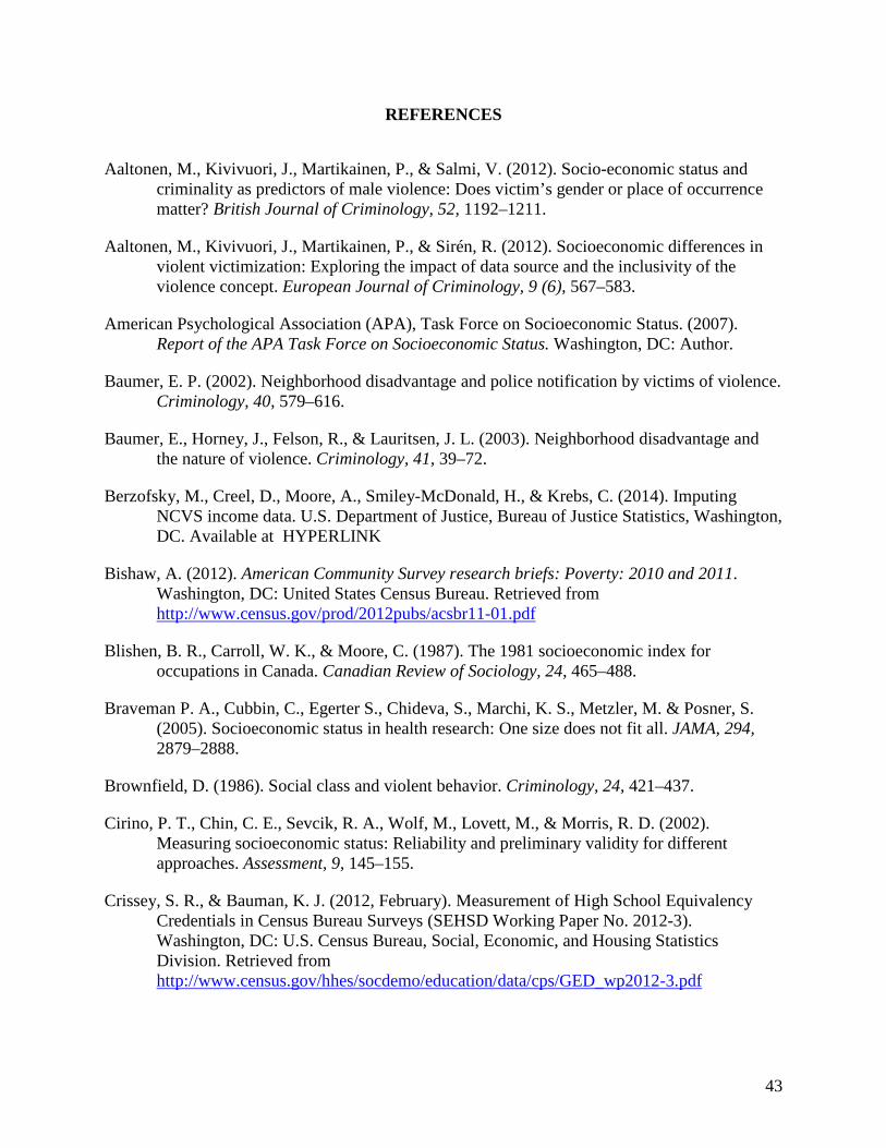
http://www.cdc.gov/nchs/ppt/nchs2012/SS-34_QUEEN.pdf

http://www.bls.gov/opub/mlr/2010/10/precis.pdf


43

REFERENCES

Aaltonen, M., Kivivuori, J., Martikainen, P., & Salmi, V. (2012). Socio-economic status and criminality as predictors of male violence: Does victim’s gender or place of occurrence matter? British Journal of Criminology, 52, 1192–1211.

Aaltonen, M., Kivivuori, J., Martikainen, P., & Sirén, R. (2012). Socioeconomic differences in violent victimization: Exploring the impact of data source and the inclusivity of the violence concept. European Journal of Criminology, 9 (6), 567–583.

American Psychological Association (APA), Task Force on Socioeconomic Status. (2007). Report of the APA Task Force on Socioeconomic Status. Washington, DC: Author.

Baumer, E. P. (2002). Neighborhood disadvantage and police notification by victims of violence. Criminology, 40, 579–616.

Baumer, E., Horney, J., Felson, R., & Lauritsen, J. L. (2003). Neighborhood disadvantage and the nature of violence. Criminology, 41, 39–72.

Berzofsky, M., Creel, D., Moore, A., Smiley-McDonald, H., & Krebs, C. (2014). Imputing NCVS income data. U.S. Department of Justice, Bureau of Justice Statistics, Washington, DC. Available at HYPERLINK

Bishaw, A. (2012). American Community Survey research briefs: Poverty: 2010 and 2011. Washington, DC: United States Census Bureau. Retrieved from http://www.census.gov/prod/2012pubs/acsbr11-01.pdf

Blishen, B. R., Carroll, W. K., & Moore, C. (1987). The 1981 socioeconomic index for occupations in Canada. Canadian Review of Sociology, 24, 465–488.

Braveman P. A., Cubbin, C., Egerter S., Chideva, S., Marchi, K. S., Metzler, M. & Posner, S. (2005). Socioeconomic status in health research: One size does not fit all. JAMA, 294, 2879–2888.

Brownfield, D. (1986). Social class and violent behavior. Criminology, 24, 421–437.

Cirino, P. T., Chin, C. E., Sevcik, R. A., Wolf, M., Lovett, M., & Morris, R. D. (2002). Measuring socioeconomic status: Reliability and preliminary validity for different approaches. Assessment, 9, 145–155.

Crissey, S. R., & Bauman, K. J. (2012, February). Measurement of High School Equivalency Credentials in Census Bureau Surveys (SEHSD Working Paper No. 2012-3). Washington, DC: U.S. Census Bureau, Social, Economic, and Housing Statistics Division. Retrieved from http://www.census.gov/hhes/socdemo/education/data/cps/GED_wp2012-3.pdf

http://www.census.gov/prod/2012pubs/acsbr11-01.pdf

http://www.census.gov/hhes/socdemo/education/data/cps/GED_wp2012-3.pdf

44

Cubbin, C., LeClere, F. B., & Smith, G. S. (2000). Socioeconomic status and injury mortality: individual and neighborhood determinants. Journal of Epidemiology and Community Health, 54, 517–524.

Demissie, K., Hanley, J. A., Menzies, D., Joseph, L., & Ernst, P. (2000). Agreement in measuring socio-economic status: Area-based versus individual measures. Chronic Diseases in Canada, 21(1).

Deonandan, R., Campbell, K., Ostbye, T., Tummon, I., & Robertson, J. (2000). A comparison of methods for measuring socio-economic status by occupation or postal area. Chronic Diseases in Canada, 21(3).

Diez-Roux, A. V. (1998). Bringing context back into epidemiology: variables and fallacies in multilevel analysis. American Journal of Public Health, 88, 216–222.

Duncan, O. D. (1961). A socioeconomic index for all occupations. In J. Reiss, Jr. (Ed.), Occupations and social status (pp. 109–138). New York, NY: Free Press of Glencoe.

Ewert, S. (2012, February). What it’s worth: Field of training and economic status in 2009. Current Population Reports, Household Economic Studies (No. P70-129). Washington, DC: U.S. Census Bureau. Retrieved from http://www.census.gov/prod/2012pubs/p70-129.pdf

Faergemann, C., Lauritsen, J. M., Brink, O., Skov, O., & Mortensen, P. B. (2009). Demographic and socioeconomic risk factors of adult violent victimization from an accident and emergency department and forensic medicine perspective: A register-based case-control study. Journal of Forensic and Legal Medicine, 16, 11–17.

Field, C.A., & Caetano, R. (2004). Ethnic differences in intimate partner violence in the U.S. general population. Trauma, Violence, & Abuse, 5(4), 303–317.

Flatley, J., Kershaw, C., Smith, K., Chaplin, R., & Moon, D. (Eds.). (2010). Crime in England and Wales 2009/10. Findings from the British Crime Survey and police recorded crime (3rd ed.). London, UK: Home Office.

Fujishiro, K., Xu, J., & Gong, F. (2010). What does “occupation” represent as an indicator of socioeconomic status: Exploring occupational prestige and health. Social Science & Medicine, 71, 2100–2107.

Hollingshead, A. B. (1975). Four factor index of social status. New Haven, CT: Department of Sociology, Yale University.

Home Office. (2011, October). User guide to Home Office crime statistics. Home Office Statistics, London, United Kingdom. Retrieved from http://www.homeoffice.gov.uk/publications/science-research-statistics/research-statistics/crime-research/user-guide-crime-statistics/user-guide-crime-statistics?view=Binary

http://www.census.gov/prod/2012pubs/p70-129.pdf

http://www.census.gov/prod/2012pubs/p70-129.pdf

http://www.homeoffice.gov.uk/publications/science-research-statistics/research-statistics/crime-research/user-guide-crime-statistics/user-guide-crime-statistics?view=Binary



45

Kassis, W., Artz, S., Scambor, C., Scambor, E., & Moldenhauer, S. (2012). Finding the way out: A non-dichotomous understanding of violence and depression resilience of adolescents who are exposed to family violence. Child Abuse & Neglect. Advance online publication. doi:10.1016/j.chiabu.2012.11.001

Khalifeh, H., Hargreaves, J., Howard, L. M., & Birdthistle, I. (2013). Intimate partner violence and socioeconomic deprivation in England: Findings from a national cross-sectional survey. American Journal of Public Health, 103, 462–472.

Kington, R. S., & Smith, J. P. (1997). Socioeconomic status and racial and ethnic differences in functional status associated with chronic diseases. American Journal of Public Health, 87, 805–810.

Kiss, L., Schraiber, L. B., Heise, L., Zimmerman, C., Gouveia, N., & Watts, C. (2012). Gender-based violence and socioeconomic inequalities: Does living in more deprived neighbourhoods increase women’s risk of intimate partner violence? Social Science & Medicine, 74, 1172–1179.

Lauritsen, J. L. (2001). The social ecology of violent victimization: Individual and contextual effects in the NCVS. Journal of Quantitative Criminology, 17, 3–32.

Lewis, G., Rice, F., Harold, G.T., Collishaw, S., & Thapar, A. (2011). Investigating environmental links between parent depression and child depressive/anxiety symptoms using an assisted conception design. Journal of the American Academy of Child & Adolescent Psychiatry, 50(5), 451–459.

Magklara, K., Skapinakis, P., Gkatsa, T., Bellos, S., Araya, R., Styliandis, S., & Mavreas, V. (2012). Bullying behavior in schools, socioeconomic position, and psychiatric morbidity: A cross-sectional study in late adolescents in Greece. Child and Adolescent Psychiatry and Mental Health, 6, 8.

Markowitz, F. E. (2003). Socioeconomic disadvantage and violence: Recent research on culture and neighborhood control as explanatory mechanisms. Aggression and Violent Behavior, 8, 145–154.

McLaughlin, K. A., Costello, J. E., Leblanc, W., Sampson, N. A., & Kessler, R. C. (2012). Socioeconomic status and adolescent mental disorders. American Journal of Public Health. Advance online publication. doi:10.2105/AJPH.2011.300477

Menard, S., Morris, R. G., Gerber, J., & Covey, H. C. (2011). Distribution and correlates of self-reported crimes of trust. Deviant Behavior, 32, 877–917.

Morenoff, J. D., Sampson, R. J., & Raudenbush, S. W. (2001). Neighborhood inequality, collective efficacy, and the spatial dynamics of urban violence. Criminology, 39, 517–560.

46

Nakao, K., & Treas, J. (1994). Updating occupational prestige and socioeconomic scores: How the new measures measure up. In P. Marsden (Ed.), Sociological methodology 1994. Washington, DC. American Sociological Association. Available from http://depts.washington.edu/socmeth2/

National Center for Health Statistics. (2012). Multiple imputation of family income and personal earnings in the National Health Interview Survey: Methods and examples. Atlanta, GA: Centers for Disease Control and Prevention. Retrieved from http://www.cdc.gov/nchs/data/nhis/tecdoc11.pdf

National Research Council. (1994). Understanding and Preventing Violence, Volume 3: Social Influences. Washington, DC: The National Academies Press.

Nilsson, A., & Estrada, F. (2006). The inequality of victimization: Trends in exposure to crime among rich and poor. European Journal of Criminology, 3, 387–412.

Oakes, J. M., & Rossi, P.H. (2003). The measurement of SES in health research: Current practice and steps toward a new approach. Social Science & Medicine, 56, 769–784.

Page, L., & Twist, N. (2011). 2010/2011 Scottish Crime and Justice Survey: Technical report. Edinburgh, Scotland: Scottish Government Social Research. Retrieved from http://www.scotland.gov.uk/Resource/Doc/933/0122908.pdf

Pineo, P. C., Porter, J., & McRoberts, H. A. (1977). The 1971 census and the socioeconomic misclassification of occupations. Canadian Review of Sociology, 14, 91–102.

Pleis, J. R., & Cohen, R. A. (2007). Impact of income bracketing on poverty measures used in the National Health Interview Survey’s (NHIS) Early Release Program: Preliminary data from the 2007 NHIS. Retrieved from http://www.cdc.gov/nchs/data/nhis/income.pdf

Precis: Labor market returns of the GED. (2010, October). Monthly Labor Review, 88–89. Retrieved from http://www.bls.gov/opub/mlr/2010/10/precis.pdf

Rennison, C., & Planty, M. (2003). Nonlethal intimate partner violence: Examining race, gender, and income patterns. Violence and Victims, 18, 433–443.

Scottish Government. (2012, December). Scottish Index of multiple deprivation 2012: A National Statistics publication for Scotland. Edinburgh, Scotland: Author. Retrieved from http://22fa0f74501b902c9f11-8b3fbddfa1e1fab453a8e75cb14f3396.r26.cf3. rackcdn.com/simd_448749_v7_20121217.pdf

Shavers, V. L. (2007). Measurement of socioeconomic status in health disparities research. Journal of the National Medical Association, 99, 1013–1023.

http://depts.washington.edu/socmeth2/

http://www.cdc.gov/nchs/data/nhis/tecdoc11.pdf

http://www.scotland.gov.uk/Resource/Doc/933/0122908.pdf

http://www.cdc.gov/nchs/data/nhis/income.pdf


http://22fa0f74501b902c9f11-8b3fbddfa1e1fab453a8e75cb14f3396.r26.cf3.rackcdn.com/simd_448749_v7_20121217.pdf

http://22fa0f74501b902c9f11-8b3fbddfa1e1fab453a8e75cb14f3396.r26.cf3.rackcdn.com/simd_448749_v7_20121217.pdf

47

Sondik, E. J., Madans, J. H., & Gentleman, J. F. (2012). Summary health statistics for U.S. adults: National Health Interview Survey, 2011. Hyattsville, MD: U.S. Department of Health and Human Services, Centers for Disease Control and Prevention, National Center for Health Statistics. Retrieved from http://www.cdc.gov/nchs/data/series/sr_10/sr10_256.pdf

Spriggs, A. L., Tucker Halpern, C., Herring, A. H., & Schoenbach, V. J. (2009). Family and school socioeconomic disadvantage: Interactive influences on adolescent dating violence victimization. Social Science & Medicine, 68, 1956–1965.

Sudman, S., & Bradburn, R. (1982). Asking questions: A practical guide to questionnaire design. San Francisco, CA: Jossey-Bass.

Szreter, S. R. S. (1984). The genesis of the Registrar General’s social classification of occupations. British Journal of Sociology, 35, 523–546.

Thacher, D. (2004). The rich get richer and the poor get robbed: Inequality in U.S. criminal victimization, 1974–2000. Journal of Quantitative Criminology, 20, 89–116.

U.S. Census Bureau. (2010, March). Observations from the Interagency Technical Working Group on developing a supplemental poverty measure. Washington, DC: Author. Retrieved from http://www.census.gov/hhes/www/poverty/SPM_TWGObservations.pdf

U.S. Census Bureau. (2011). American FactFinder: Table S1901: Income in the past 12 months (in 2011 inflation-adjusted dollars). Retrieved from http://factfinder2.census.gov/faces/tableservices/jsf/pages/productview.xhtml?pid=ACS_11_1YR_S1901&prodType=table

U.S. Census Bureau. (2012a). Description of income and poverty data sources. Washington, DC: Author. Retrieved from http://www.census.gov/hhes/www/ poverty/about/datasources/description.html#sippbckgrnd

U.S. Census Bureau. (2012b). How the Census Bureau measures poverty. Washington, DC: Author. Retrieved from http://www.census.gov/hhes/www/poverty/about/ overview/measure.html

Van Kesteren, J., Mayhew, P., & Nieuwbeerta, P. (2000). Criminal victimization in seventeen industrialised countries: Key findings from the 2000 International Crime Victims Survey. The Hague, The Netherlands: Ministry of Justice, WODC [Research and Documentation Center].

Winnersjö, R., Ponce de Leon, A., Soares, J. F., & Macassa, G. (2012). Violence and self-reported health: Does individual socio-economic position matter? Journal of Injury and Violence Research, 4, 87–95.

Xie, M., Heimer, K., & Lauritsen, J. L. (2012). Violence against women in U.S. metropolitan areas: Changes in women’s work status and work. Criminology, 50, 105–143.

http://www.cdc.gov/nchs/data/series/sr_10/sr10_256.pdf

http://www.census.gov/hhes/www/poverty/SPM_TWGObservations.pdf

http://factfinder2.census.gov/faces/tableservices/jsf/pages/productview.xhtml?pid=ACS_11_1YR_S1901&prodType=table

http://factfinder2.census.gov/faces/tableservices/jsf/pages/productview.xhtml?pid=ACS_11_1YR_S1901&prodType=table

http://www.census.gov/hhes/www/poverty/about/datasources/description.html%23sippbckgrnd

http://www.census.gov/hhes/www/poverty/about/datasources/description.html%23sippbckgrnd

http://www.census.gov/hhes/www/poverty/about/overview/measure.html


48

Yabroff, K. R., & Gordis, L. (2003). Assessment of National Health Interview Survey-based method of measuring community socioeconomic status. Annals of Epidemiology, 13, 721–726.

Zinzow, H. M., Ruggiero, K. J., Resnick, H., Hanson, R., Smith, D., Saunders, B., & Kilpatrick, D. (2009). Prevalence and mental health correlates of witnessed parental and community violence in a national sample of adolescents. Journal of Child Psychology and Psychiatry, 50, 441–540.

49

APPENDIX A: REFERENCED TABLES

Table A-1. Description of how socioeconomic status is measured in selected studies

Survey agency

Panel design? Description of the socioeconomic status data that are used

Current Population Survey (CPS) Bureau of Labor Statistics; Census Bureau

Y Overview: The CPS focuses on “poverty status,” which is derived by examining the data from a series of questions from more than 50 sources of income during the previous calendar year.a Under the Office of Management and Budget’s (OMB’s) Statistical Policy Directive 14 guideline, the CPS uses a set of money income thresholds that vary by family size and composition to detect who is poor. Poverty Status Measures: Income includes earnings, unemployment compensation, workers’ compensation, Social Security, Supplemental Security Income (SSI), public assistance, veterans’ payments, survivor benefits, pension or retirement income, interest, dividends, rents, royalties, income from estates, trusts, educational assistance, alimony, child support, assistance from outside the household, and other miscellaneous sources.b Noncash benefits (e.g., food stamps) do not count, and income is measured before taxes and excludes capital gains and losses. The questionnaire provides categorical responses for total income spanning 16 different income ranges, beginning with “Less than $5,000” and ending with “$150,000 or more.” Poverty thresholds are the dollar amounts used to determine poverty status that do not vary geographically but are updated annually for inflation with the Consumer Price Index for All Urban Consumers (CPI-U). Each person or family is assigned one of 48 possible poverty thresholds.b Computation: If total family income is less than the threshold appropriate for that family, the family is in poverty, and all family members have the same poverty status. If total family income equals or exceeds the threshold, the family is not in poverty. For more information about the poverty measure, access http://www.census.gov/hhes/www/poverty/about/overview/measure.html. Other Approaches: Recently, the Census Bureau has begun reporting the “Supplemental Poverty Measure,” which derives poverty thresholds from the Consumer Expenditure Survey on basic necessities (food, shelter, clothing, and utilities) and is adjusted for geographic differences in the cost of housing.c It is not intended to replace the official poverty measure but is supposed to provide an additional indicator of economic well-being and provide a better understanding of economic conditions and policy impacts.c For more information on the Supplemental Poverty Measure, access http://www.census.gov/hhes/www/poverty/SPM_TWGObservations.pdf.

(continued)

http://www.census.gov/hhes/www/poverty/data/threshld/thresh10.xls



50

Table A-1. Description of how socioeconomic status is measured in selected studies (continued)

Survey agency


Survey of Income and Program Participation (SIPP) Census Bureau

Y Overview: The SIPP collects monthly income for up to 81 sources of income and up to 73 individual income values.d SIPP estimates of annual income and annual poverty can be obtained by summing 12 months of family income and monthly poverty thresholds, both of which may vary month to month. Like the CPS, the SIPP uses a set of thresholds that vary by family size and composition to determine the poverty status of a household. If a family’s total income is less than that family’s threshold, then the family and every individual within it are considered to be in poverty.e Poverty Status Measures: At the individual level, income includes earned income, unearned or property income, and transfer program income.f Earned income comprises wage and salary income, self-employed earnings, and earnings from other work arrangements. Unearned or property income refers to all income generated from interest, dividends, lump-sum payments from insurance claims, and payments from annuities and retirement, as well as payments from trusts, estates, and royalties. Transfer program income refers to cash payments from social welfare programs, SSI, Temporary Assistance to Needy Families, and general assistance. Poverty thresholds are the dollar amounts used to determine poverty status. Each person or family is assigned one of 48 possible poverty thresholds. Thresholds vary according to the size of the family and the ages of the members. The same thresholds are used throughout the United States (i.e., they do not vary geographically) and are updated annually using the CPI-U. Computation: In the SIPP, because income is reported multiple times a year, annual poverty rates are calculated using the sum of family income over the year divided by the sum of poverty thresholds, which can change from month to month if one’s family composition changes.g Notably, in one recent SIPP study,h the small portion of families reporting zero average monthly income for the year were excluded from the analysis because of concerns that “fixing it” would introduce bias because of the small proportion of households reporting zero income and the unlikelihood of a family with no annual income. Other Approaches: Beyond the computation that would be derived under OMB’s Directive 14 (as described above), the Census Bureau (Anderson, 2011) has also examined poverty in other ways using the SIPP panel data, including the following: Monthly Poverty Rate—Percentage in poverty in a given month using monthly income and a monthly threshold. Episodic Poverty Rate—Percentage in poverty for 2 or more consecutive months. Chronic Poverty Rate—Percentage in poverty every month of the time frame being considered. Length of Poverty Spell—Number of months in poverty. The minimum spell length is 2 months, and spells are separated by 2 or more months of not being in poverty. Individuals can have more than one spell. Spells under way in the first interview month of the panel are excluded. Poverty Entry—On the basis of the annual poverty measures, people who were not in poverty in the first year of the panel but in poverty in one or more subsequent years. Poverty Exit—On the basis of the annual poverty measure, people who were in poverty in the first year of the panel but not in poverty in one or more subsequent years.

(continued)



51


Survey agency


Panel Study of Income Dynamics (PSID) National Science Foundation, National Institute on Aging, and Eunice Kennedy Shriver National Institute of Child Health & Human Development

Y Overview: Like the CPS, the PSID uses threshold poverty values to assess socioeconomic well-being on the basis of combined family income, family size, the number of persons in the family under age 18, and the ages of the household members.i Poverty Status Measures: The “Total Family Income” variable is created for each data collection wave and represents an aggregation of all labor, asset, and government transfer income (cash welfare, Social Security, etc.) for the head, spouse, and all others living in the family unit at any point during the calendar year (Institute for Social Research, 2012). PSID family income reflects the income of all persons living in the family unit during calendar year t, regardless of whether that person was living in the family at the time of the interview in year t+1. Income for each family member includes only the amount accrued during the months that the person resided with the other family members. Notably, the PSID defines “family” more broadly and includes unrelated people who live together and share resources (like cohabiting partners). The broad income categories include head and wife taxable income; head and wife transfer income; other family member taxable income; other family member transfer income; head and wife Social Security income; and other family member Social Security income. In addition, respondents are asked to provide detailed information for each of the head’s and wife’s jobs. The employment data are combined with the income data to compute a wage rate for both the head and wife, and may also be used for imputing labor income when needed (Institute for Social Research, 2012). Computation: Variables representing the total value of wealth and its major subcomponents are used to derive an overall wealth indicator (Institute for Social Research, 2012).

American Community Survey (ACS) Census Bureau

N Overview: Using a series of eight questions, the ACS asks about money income, plus one type of noncash benefit (food stamps), during the previous 12 months. ‘‘Total income’’ is the sum of the amounts reported separately for wage or salary income; net self-employment income; interest, dividends, net rental or royalty income, or income from estates and trusts; Social Security or railroad retirement income; SSI; public assistance or welfare payments; retirement, survivor, or disability pensions; and all other income. The estimates are adjusted for inflation using the Consumer Price Index.j Poverty Status Measures. Poverty statistics in ACS products adhere to the standards specified by OMB Directive 14. The Census Bureau uses a set of dollar value thresholds that vary by family size and composition to determine who is in poverty. Furthermore, poverty thresholds for people living alone or with nonrelatives (unrelated individuals) vary by age (under 65 years or 65 years and older). The poverty thresholds for two-person families also vary by the age of the householder. If a family’s total income is less than the dollar value of the appropriate threshold, then that family and every individual in it are considered to be in poverty. Similarly, if an unrelated individual’s total income is less than the appropriate threshold, then that individual is considered to be in poverty (Bishaw, 2012). Computation. In determining the poverty status of families and unrelated individuals, the Census Bureau uses thresholds (income cutoffs) arranged in a two-dimensional matrix. The matrix consists of family size (from one person to nine or more people) cross-classified by presence and number of family members under 18 years old (from no children present to eight or more children present). Unrelated individuals and two-person families are further differentiated by age of reference person (under 65 years old and 65 years old and over).

(continued)

52


Survey agency


To determine a person’s poverty status, the person’s total family income in the last 12 months is compared with the poverty threshold appropriate for that person’s family size and composition. If the total income of that person’s family is less than the threshold appropriate for that family, then the person is considered “below the poverty level,” together with every member of his or her family. If a person is not living with anyone related by birth, marriage, or adoption, then the person’s own income is compared with his or her poverty threshold. The total number of people below the poverty level is the sum of people in families and the number of unrelated individuals with incomes in the last 12 months below the poverty threshold (Bishaw, 2012).

a U.S. Census Bureau. (2012a). Description of income and poverty data sources. Washington, DC: Author. Retrieved from http://www.census.gov/hhes/www/poverty/about/ datasources/description.html#sippbckgrnd.

b U.S. Census Bureau. (2012b). How the Census Bureau measures poverty. Washington, DC: Author. Retrieved from http://www.census.gov/hhes/www/poverty/about/ overview/measure.html

c U.S. Census Bureau. (2010, March). Observations from the Interagency Technical Working Group on developing a supplemental poverty measure. Washington, DC: Author. Retrieved from http://www.census.gov/hhes/www/poverty/SPM_TWGObservations.pdf

d U.S. Census Bureau. (2012a). Description of income and poverty data sources. Washington, DC: Author. Retrieved from http://www.census.gov/hhes/www/poverty/about/ datasources/description.html#sippbckgrnd

e Anderson, R. J. (2011, March). Dynamics of economic well-being: Poverty 2004–2006 (Current Population Reports No. P70-123). Washington, DC: United States Census Bureau. Retrieved from http://www.census.gov/hhes/www/poverty/publications/dynamics04/P70-123.pdf

f Westat. (2001). Survey of Income and Program Participation users’ guide (3rd ed.). Washington, DC: Author. Retrieved from http://www.census.gov/sipp/usrguide/ sipp2001.pdf

g U.S. Census Bureau. (2012a). Description of income and poverty data sources. Washington, DC: Author. Retrieved from http://www.census.gov/hhes/www/poverty/about/ datasources/description.html#sippbckgrnd

h Hisnanick, J. J. (2007). The dynamics of low income and persistent poverty among U.S. families. Journal of Income Distribution, 16(1), 116–132. i Institute for Social Research, University of Michigan. (2012). PSID main interview user manual (Release 2012.1). Ann Arbor, MI: Author. Retrieved from

http://psidonline.isr.umich.edu/data/Documentation/UserGuide2009.pdf j Bishaw, A. (2012). American Community Survey research briefs: Poverty: 2010 and 2011. Washington, DC: United States Census Bureau. Retrieved from


http://www.census.gov/hhes/www/poverty/about/%20datasources/description.html%23sippbckgrnd


http://www.census.gov/hhes/www/poverty/about/%20overview/measure.html

http://www.census.gov/hhes/www/poverty/about/%20overview/measure.html




http://www.census.gov/hhes/www/poverty/publications/dynamics04/P70-123.pdf

http://www.census.gov/sipp/usrguide/%20sipp2001.pdf

http://www.census.gov/sipp/usrguide/%20sipp2001.pdf



http://psidonline.isr.umich.edu/data/Documentation/UserGuide2009.pdf


53

Table A-2. Victimization rates by type of crime and household income, 2010

Household income Number of households Percentage

Rape and sexual assault Robbery

Aggregated assault

Simple assault

All violent crimes

Household burglary

Motor vehicle theft

All property crimes

Less than $15,000 17,185,600 14.0% 1.6 4.0 5.6 17.2 28.4 45.6 4.4 159.3 $15,000–$34,999 30,206,400 24.6 0.8 3.0 4.2 14.9 22.9 29.0 5.5 132.2 $35,000–$49,999 19,406,900 15.8 0.8* 1.9 4.5 11.0 18.2 25.2 4.6 121.6 $50,000–$74,999 20,965,200 17.1 1.6 2.2 2.2 11.6 17.6 18.5 5.5 109.8 $75,000 or more 35,121,200 28.6 0.8* 1.2 2.0 10.9 14.9 18.2 4.5 114.4

Note: Rate per 1,000. *Interpret with caution; estimate based on 10 or fewer sample cases or coefficient of variation is greater than 50%. Source: Bureau of Justice Statistics National Crime Victimization Survey (NCVS), 2010. Table A-3. Victimization rates by type of crime and household income as percentage of Federal poverty level, 2010

Household income (percentage of

Federal poverty level)



Aggregated assault

Simple assault

All violent crimes

Household burglary

Motor vehicle theft

All property crimes

100% or less 16,979,800 13.8% 1.8 5.0 5.8 16.8 29.5 45.4 6.3 179.8 101%–150% 12,226,600 10.0 0.7* 3.3 4.5 15.1 23.6 37.5 7.3 166.6 151%–200% 11,842,100 9.6 1.1* 1.9 3.2 16.3 22.5 29.7 4.0 129.9 201%–300% 21,132,500 17.2 0.7* 2.6 4.1 12.3 19.6 23.3 4.0 117.2 301%–400% 15,335,100 12.5 1.8* 1.0 2.2 14.0 19.0 18.9 4.4 103.6 401%–500% 10,564,000 8.6 --* 0.7* 2.3 14.6 17.8 14.0 6.4 97.1 Greater than 500% 34,805,100 28.3 0.9* 1.3 2.1 7.5 11.7 19.1 4.1 106.0

Note: Rate per 1,000. *Interpret with caution; estimate based on 10 or fewer sample cases or coefficient of variation is greater than 50%. *Interpret with caution; estimate based on 10 or fewer sample cases or coefficient of variation is greater than 50%. — Number less than 0.5. Source: Bureau of Justice Statistics National Crime Victimization Survey (NCVS), 2010.

54

Table A-4. Victimization rates by type of crime and education level, 2010

Education level Number of

persons Percentage


Aggregated assault

Simple assault

All violent crimes

Household burglary

Motor vehicle theft

All property crimes

Less than high school 59,533,500 23.3% 1.5 2.5 5.6 14.2 23.8 43.5 5.7 211.7 High school, some college, or associate’s degree

128,207,600 50.1 1.2 2.6 3.0 13.8 20.6 27.7 5.3 128.0

Bachelor’s degree 43,868,200 17.1 —* 1.6 2.1 10.6 14.5 16.9 4.5 89.5 Master’s, professional, or doctoral degree

18,609,800 7.3 0.5* 1.0* 2.6* 6.6 10.7 16.8 2.8* 103.5

Unknown 5,742,800 2.2 —* 0.8* —* 7.0* 7.8 12.1 3.2* 53.2

Note: Rate per 1,000. *Interpret with caution; estimate based on 10 or fewer sample cases or coefficient of variation is greater than 50%. — Number rounds to less than 0.5. Source: Bureau of Justice Statistics National Crime Victimization Survey (NCVS), 2010. Table A-5. Victimization rates by type of crime and 6-month employment status, 2010

Employment status Number of

persons Percentage


Aggregated assault

Simple assault

All violent crimes

Household Burglary

Motor vehicle theft

All property crimes

Employed 146,617,000 57.3% 1.1 2.3 2.9 14.3 20.6 51.6 11.8 265.8 Unemployed 90,474,400 35.4 0.7 2.2 3.6 9.5 16.0 14.6 1.9 58.3 Unknown† 18,870,500 7.4 2.4* 1.6* 6.1 14.8 24.9 16.9* 2.1* 391.5

Note: Rate per 1,000. *Interpret with caution; estimate based on 10 or fewer sample cases or coefficient of variation is greater than 50%. †Includes those under 18 years old. Source: Bureau of Justice Statistics National Crime Victimization Survey (NCVS), 2010.

55

Table A-6. Victimization rates by type of crime and housing tenure, 2010

Tenure Number of households Percentage


Aggregated assault

Simple assault

All violent crimes

Household burglary

Motor vehicle theft

All property crimes

Own 82,203,700 66.9% 0.6 1.0 2.0 8.4 12.0 21.1 3.7 103.6 Rent or no cash rent 40,681,400 33.1 2.0 5.1 6.4 22.6 36.1 35.5 7.5 169.4

Note: Rate per 1,000. Source: Bureau of Justice Statistics National Crime Victimization Survey (NCVS), 2010. Table A-7. Victimization rates by type of crime and public housing status, 2010

Public housing Number of households Percentage


Aggregated assault

Simple assault

All violent crimes

Household burglary

Motor vehicle theft

All property crimes

No 120,201,600 97.9% 1.0 2.2 3.3 12.5 19.0 25.4 4.9 125.0 Yes 2,630,200 2.1 1.7* 5.9* 3.3* 25.4 36.2 46.8 5.7* 143.6

Note: Rate per 1,000. *Interpret with caution; estimate based on 10 or fewer sample cases or coefficient of variation is greater than 50%. Source: Bureau of Justice Statistics National Crime Victimization Survey (NCVS), 010.

56

Table A-8. Crosstab of persons by income level and employment status, 2010

Income (percentage of Federal poverty level)

Employment status

No (%) Yes (%)

100% or less 53.2 46.8 101% to 200% 46.4 53.7 201% to 400% 35.4 64.6 401% or greater 26.3 73.7


Table A-9. Crosstab of persons by income level and household tenure, 2010

Income

Household tenure

Rent (%) Own (%) 100% or less 58.5 41.5 101% to 200% 41.0 59.0 201% to 400% 26.2 73.8 401% or greater 17.0 83.0


Table A-10. Crosstab of persons by income level and public housing status, 2010

Income

Public housing

Yes (%) No (%) 100% or less 6.0 94.0 101% to 200% 2.4 97.6 201% to 400% 0.7 99.3 401% or greater 0.3 99.7


Table A-11. Crosstab of persons by income level and education level, 2010

Income

Education

Less than high school (%)

High school, some college, or

associate’s degree (%)

Bachelor’s degree (%)

Master’s, professional, or doctoral degree

(%)

100% or less 32.4 57.3 8.0 2.3

101% to 200% 24.7 63.0 9.8 2.6

201% to 400% 13.4 62.7 18.1 5.9

401% or greater 6.8 47.9 29.9 15.4


57

Table A-12. Crosstab of persons by education level and employment status, 2010

Education

Employment status

No (%) Yes (%)

Less than high school 55.3 44.7 High school, some college, or associate’s degree 37.1 62.9 Bachelor’s degree 24.6 75.4 Master’s, professional, or doctoral degree 23.6 76.4


Table A-13. Crosstab of persons by education level and household tenure, 2010

Education

Household tenure

Rent (%) Own (%)



Table A-14. Crosstab of persons by education level and public housing status, 2010

Education

Public housing

Yes (%) No (%)



Table A-15. Crosstab of persons by household tenure and employment status, 2010

Household tenure

Employment status

No (%) Yes (%)

Rent 35.7 64.3 Own 37.0 63.0


58

Table A-16. Victimization rates by type of crime and SES Index 1, 2010

SES Index 1 categories†



Aggregated assault

Simple assault

All violent crimes

Household burglary

Motor vehicle theft

All property crimes

1 2,436,200 2.0 0.9* 1.0* 15.8 18.9 36.6 49.4 9.6* 171.2 2 7,222,600 5.9 1.8* 5.3 5.1 19.0 31.2 49.3 5.9 182.4 3 12,662,800 10.3 1.3* 5.2 5.0 18.2 29.7 39.7 6.5 178.1 4 17,003,500 13.8 1.3 2.4 3.9 12.9 20.4 33.0 5.1 144.2 5 21,703,300 17.7 1.6 2.1 3.5 14.2 21.5 27.7 4.9 128.5 6 23,446,500 19.1 --* 1.7 1.7 12.8 16.4 16.5 5.0 101.5 7 20,783,400 16.9 1.1* 0.8 3.2 8.9 14.0 19.9 4.3 107.7 8 13,641,300 11.1 --* 0.8* 1.3* 6.7 9.3 14.8 3.6 102.8

Unknown 3,985,600 3.2 --* 1.8* --* 3.9* 6.2 8.7 2.4* 40.4

Note: Rate per 1,000. †The Socioeconomic Status (SES) Index does not result in whole numbers. The categories represent the results as follows: 1 = 0 to less than 1, 2 = 1 to less than 2, 3 = 2 to less

than 3, 4 = 3 to less than 4, 5 = 4 to less than 5, 6 = 5 to less than 6, 7 = 6 to less than 7, and 8 = 7 to 8. *Interpret with caution; estimate based on 10 or fewer sample cases or coefficient of variation is greater than 50%. — Number less than 0.5. Source: Bureau of Justice Statistics National Crime Victimization Survey (NCVS), 2006–2010.





Aggregated assault

Simple assault

All violent crimes

Household burglary

Motor vehicle theft

All property crimes

1 466,700 0.4 2.4* 2.5* --* 14.0* 19.0* 28.0* 11.5* 113.1 2 4,148,200 3.4 1.3* 2.1* 9.8 17.7 30.8 49.0 7.4* 157.1 3 10,628,100 8.7 1.1* 4.3 5.9 15.1 26.3 48.5 5.2 174.5 4 17,103,400 13.9 1.2 3.6 3.1 13.2 21.1 32.2 5.3 151.4 5 21,475,200 17.5 1.0 2.2 3.8 14.5 21.6 27.4 5.6 133.3 6 25,504,200 20.8 1.3* 1.7 2.5 14.3 19.8 21.8 3.8 113.4 7 23,336,500 19.0 1.1* 1.5 2.1 10.3 15.0 18.9 5.2 110.0 8 16,200,600 13.2 0.5* 1.0 2.9 8.2 12.7 16.6 4.8 108.9

Unknown 4,022,200 3.3 --* 2.2* 0.8* 3.8* 6.8 8.7 2.3* 43.2 Note: Rate per 1,000. †The Socioeconomic Status (SES) does not result in whole numbers. The categories represent the results as follows: 1 = 0 to less than 1, 2 = 1 to less than 2, 3 = 2 to less than 3, 4

= 3 to less than 4, 5 = 4 to less than 5, 6 = 5 to less than 6, 7 = 6 to less than 7, and 8 = 7 to 8. *Interpret with caution; estimate based on 10 or fewer sample cases or coefficient of variation is greater than 50%. — Number less than 0.5. Source: Bureau of Justice Statistics National Crime Victimization Survey (NCVS), 2010.

59





Aggregated assault

Simple assault

All violent crimes

Household burglary

Motor vehicle theft

All property crimes

1 3,810,100 3.1 0.9* 1.2* 10.0 16.4 28.5 42.1 7.0* 147.2 2 10,795,900 8.8 1.3* 4.2 5.6 15.5 26.6 50.7 6.0 175.5 3 17,389,400 14.2 1.2 3.9 3.3 13.4 21.7 31.4 5.2 152.7 4 21,643,700 17.6 1.0 2.2 3.9 13.5 20.6 28.6 5.5 133.7 5 25,676,900 20.9 1.3* 1.6 2.5 15.1 20.6 21.7 3.7 113.4 6 23,368,200 19.0 1.1* 1.5 2.1 10.3 15.0 18.9 5.2 110.0 7 16,215,300 13.2 0.5* 1.0 2.9 8.2 12.7 16.6 4.8 108.9

Unknown 3,985,600 3.2 --* 1.8* --* 3.9* 6.2 8.7 2.4* 40.4 Note: Rate per 1,000. †The Socioeconomic Status (SES) does not result in whole numbers. The categories represent the results as follows: 1 = 0 to less than 1, 2 = 1 to less than 2, 3 = 2 to less than 3, 4

= 3 to less than 4, 5 = 4 to less than 5, 6 = 5 to less than 6, and 7 = 6 to 7. * Interpret with caution; estimate based on 10 or fewer sample cases or coefficient of variation is greater than 50%. — Number less than 0.5. Source: Bureau of Justice Statistics National Crime Victimization Survey (NCVS), 2010.

Documents

Measuring Socioeconomic Status (SES) in the NCVS