Embed Size (px)
Citation preview
Measuring IFAD’s impact
byAlessandra GarberoResearch and Impact Assessment Division
IFAD RESEARCHSERIES
07
Background paper to the IFAD9 Impact Assessment Initiative
The opinions expressed in this publication are those of the authors and do not necessarily represent
those of the International Fund for Agricultural Development (IFAD). The designations employed and the
presentation of material in this publication do not imply the expression of any opinion whatsoever on
the part of IFAD concerning the legal status of any country, territory, city or area or of its authorities, or
concerning the delimitation of its frontiers or boundaries. The designations “developed” and “developing”
countries are intended for statistical convenience and do not necessarily express a judgement about the
stage reached in the development process by a particular country or area.
This publication or any part thereof may be reproduced for non-commercial purposes without prior
permission from IFAD, provided that the publication or extract therefrom reproduced is attributed to IFAD
and the title of this publication is stated in any publication and that a copy thereof is sent to IFAD.
Author:Alessandra Garbero
© IFAD 2016
All rights reserved
ISBN 978-92-9072-703-3
Printed December 2016
The IFAD Research Series has been initiated by the Strategy and Knowledge Department in order to bring
together cutting-edge thinking and research on smallholder agriculture, rural development and related
themes. As a global organization with an exclusive mandate to promote rural smallholder development,
IFAD seeks to present diverse viewpoints from across the development arena in order to stimulate
knowledge exchange, innovation, and commitment to investing in rural people.
IFAD RESEARCHSERIES
07
byAlessandra GarberoResearch and Impact Assessment Division
Measuring IFAD’s impact
Background paper to the IFAD9 Impact Assessment Initiative
The author is grateful for the comments provided by IFAD colleagues, including Josefina Stubbs, Paul Winters, Rui Benfica, Tisorn Songsermsawas, Pierre Marion and Daniel Higgins, as well as colleagues from the Fund’s Independent Office of Evaluation, including Oscar Garcia, Ashwani Muthoo* and Fabrizio Felloni. The paper was also reviewed and benefited from the insights provided by David Evans, Markus Goldstein and Gero Carletto from the World Bank, and Benjamin Davis from the Food and Agriculture Organization of the United Nations (FAO).
About the authors
Alessandra Garbero is Senior Econometrician in the Research and Impact Assessment Division, Strategy and Knowledge Department, IFAD. Her work focuses on impact assessment methodologies and applied econometrics in developing regions. She obtained her PhD from the London School of Hygiene and Tropical Medicine. Her thesis, “Estimation of the impact of adult deaths on households’ welfare using panel data in KwaZulu-Natal, South Africa,” is a methodological assessment of the implications of different econometric methods used in the relevant literature to estimate the impact of adult deaths. Her first degree is in economics and she specialized in demography and research methods. Her prior work experience involved working at the United Nations Population Division on population projections and at FAO on the impact of HIV and AIDS on food security and agriculture, as well as on the improvement of the collection, dissemination and use of gender-disaggregated data in agriculture and rural development. She also developed a methodology to evaluate the impact of HIV and AIDS on the agricultural labour force. Prior to joining IFAD, she was a Research Scholar at the International Institute for Applied Systems Analysis, where she was part of a team of analysts working on analytical, methodological and modelling research.
Acknowledgements
2
* Ashwani Muthoo was appointed Director of IFAD’s Global Engagement, Knowledge and Strategy Division in April 2016.
3
Table of contents
Acknowledgements ...................................................................................................................2
Abstract ......................................................................................................................................4
Executive summary ....................................................................................................................5
Introduction ................................................................................................................................7
History of the IFAD9 agenda and its commitments .............................................................8
Data and methods: concepts and approach ...........................................................................10
Conceptual issues ..............................................................................................................11
Overall methodological approach of IFAD9 IAI ....................................................................21
Results: lessons, estimates and projections ............................................................................46
Lessons on methods ..........................................................................................................46
Estimates and projections of impacts .................................................................................47
Conclusions and proposals for moving forward ......................................................................84
Appendices ................................................................................................................................88
IFAD9 ex post impact assessments: overview of evaluation framework ..............................88
Experimental designs (RCTs) under the 3ie Agricultural Innovation Window ........................91
Sensitivity analysis to different poverty lines ........................................................................99
References .................................................................................................................................101
4
In recent years, the International Fund for Agricultural Development (IFAD) has increasingly strengthened its focus on achieving and measuring results. In 2011-2012, resources were invested in the IFAD9 Impact Assessment Initiative (IFAD9 IAI) in order to: (i) explore methodologies to assess impact; (ii) measure – to the degree possible – the results and impacts of IFAD-financed activities; and (iii) summarize lessons learned and advise on rigorous and cost-effective approaches to attributing impact to IFAD interventions. The initiative reflects a recognition of IFAD’s responsibility to generate evidence of the success of IFAD-supported projects so as to learn lessons for the benefit of future projects. This paper describes the IFAD9 IAI and the range of methods that have been identified to broaden the evidence base for the estimation of IFAD impacts, and presents the results from the aggregation and projection methodology used to compute the Fund’s aggregate impact on key outcomes, while also highlighting what has been learned. The results show that there are many areas in which IFAD-supported project beneficiaries have had, on average, better outcomes in percentage terms as compared to comparison farmers who were not project beneficiaries. Specifically, IFAD-supported projects are effectively poverty-reducing: when choosing durable asset indexes as the preferred poverty proxies on the grounds that they better approximate long-run wealth, findings point to statistically significant gains. Overall, the analyses strongly imply that IFAD is effectively improving the well-being of rural people in terms of asset accumulation, and higher revenue and income. The IFAD9 IAI represents a pioneering research effort, which has tried to overcome the clear challenges of designing data collection and conducting ex post impact assessments in a context where data were scarce, with a view to measuring progress towards a global accountability goal over a very short period of time. Therefore, an important recommendation is that future impact assessments should be selected and designed ex ante, and structured to facilitate and maximize learning, rather than used solely as an instrument to prove accountability.
Abstract
5
Executive summary
In 2011-2012, resources were invested in the IFAD9 Impact Assessment Initiative (IFAD9 IAI)
in order to: (i) explore methodologies to assess impact; (ii) measure – to the degree possible
– the results and impacts of IFAD-financed activities; and (iii) summarize lessons learned and
advise on rigorous and cost-effective approaches to attributing impact to IFAD interventions.
The initiative reflected a recognition of IFAD’s responsibility to generate evidence of the
success of IFAD projects so as to learn lessons for the benefit of future projects. The objectives
of this paper are twofold: first, to describe the IFAD9 IAI and the range of methods that have
been identified to broaden the evidence base for the estimation of IFAD impacts; and second,
to present the results from the aggregation and projection methodology used to compute the
Fund’s aggregate impact on key outcomes.
To provide estimates of IFAD’s impact, 22 ex post designed impact assessments with
non-experimental designs and involving primary data collection were completed, in
addition to 14 in-house ex post impact assessments based on existing surveys. Furthermore,
six evaluations designed ex ante using experimental methods (randomized control trials)
are currently ongoing with the aim of exploring different methodologies. Meta-analysis
was utilized with a view to aggregating results from different types of evaluations, while
attempting to control for various sources of bias linked to the heterogeneity of treatment
effects, different types of evaluation designs or, more broadly, degree of rigour (i.e. an
individual study’s external and internal validity) and the extent of measurement error.
Meta-analysis, a powerful technique designed to provide a quantitative summary of statistical
indicators reported in similar empirical studies, was used to calculate an aggregate estimate
of the Fund’s impact across a range of outcomes. The paper concludes with projections of
the Fund’s impact, as estimated from the analysed projects, to the rest of the IFAD portfolio
across a series of outcomes. The main assumption behind the method is that effect sizes are
assumed to be calculated from representative studies of IFAD projects and can be extrapolated
within mutually exclusive project categories. Following this rationale, and based on an
overall beneficiary population of approximately 240 million reached by IFAD-supported
projects that were either closing or ongoing between 2010 and 2015, projections suggest
that 44 million beneficiaries will see substantial increases in agricultural revenues, as well
as positive gains in poultry asset ownership (28.8 million) and livestock asset ownership
(22.8 million). More than 13 million beneficiaries will experience significant increases in
overall assets and productive farm assets. Positive gains (affecting around 10 million) also
occur in the realm of gender empowerment, dietary diversity and reduction in shock exposure.
Finally, using an asset-based poverty measure, an estimated 24 million beneficiaries moved
out of poverty as a result of projects that were either closing or ongoing between 2010 and
2015 (approximately 392 projects).
6
Cognizant of the methodological limitations, and of the numerous statistical or empirical assumptions made as part of this work, the IFAD9 IAI represents a pioneering research effort which has tried to overcome the clear challenges of designing data collection and conducting impact assessments ex post in a context where data were scarce, and with a view to measuring a global accountability goal over a very short period of time. Therefore, this paper points to a number of important recommendations. First, future impact assessments should be selected and structured to facilitate and maximize learning, rather than merely as instruments to prove accountability. Second, IFAD should focus on a comprehensive set of indicators that reflect the three strategic objectives articulated in its Strategic Framework, including a shift towards economic mobility indicators and a multidimensional approach to poverty. Third, creating an impact assessment agenda requires systematically reviewing the IFAD project portfolio to understand the impact potential of IFAD-funded projects, and to identify where the gaps in the evidence of the success of those projects are. Fourth, IFAD must focus on ex ante impact assessments, i.e. impact assessments that are embedded at the project design stage, given the challenges that are inherent in conducting ex post impact assessments. Sixth, the future IFAD impact assessment agenda must reflect a multi-stakeholder and participatory process, where the collaboration among research teams, project management units, IFAD staff and, more broadly, implementers must be established ex ante, i.e. at the beginning of the project.
7
The International Fund for Agricultural Development (IFAD) has been increasingly
strengthening its focus on achieving and measuring results. The Governing Council has
asked the Fund to create a comprehensive system for measuring and reporting the results
of IFAD-supported projects. Towards this end, the Results and Impact Measurement System
(RIMS) was established in 2004. While the RIMS roll-out was gradual, with delays in projects
becoming compliant and data quality being highly variable, RIMS greatly improved the
capacity of IFAD to monitor its activities and to assess its contribution towards improving the
well-being of poor rural households. Moreover, RIMS was part of a broader effort to improve
IFAD’s self-evaluation at the design, implementation and completion stages of its projects.
In fact, an independent peer review of IFAD’s Office of Evaluation and Evaluation Function,
undertaken in 2010, noted that self-evaluation was significantly strengthened at IFAD during
this period (IFAD 2010, 2011).1
While moving IFAD forward in achieving and measuring results, the RIMS data and
self-evaluation system were limited in their ability to attribute higher-order impacts of
IFAD-financed activities. The IFAD9 Impact Assessment Initiative (IFAD9 IAI) was agreed
upon between 2011 and 2012. The commitment included an “enhanced thrust on impact
evaluation,” which imposed a substantial burden on the existing systems, which at that time
were not adequately equipped for the task (IFAD 2012b). Thus, resources were invested as part
of the Ninth Replenishment of IFAD’s Resources (IFAD9) to: (i) explore methodologies to
assess impact; (ii) measure – to the degree possible – the results and impact of IFAD-financed
activities; and (iii) summarize lessons learned and advise on rigorous and cost-effective
approaches to attributing impact to IFAD interventions (IFAD 2012a).
The initiative by IFAD Management to promote an impact assessment agenda reflects the
recognition of its responsibility to generate evidence of the success of IFAD projects so as to
learn lessons for the benefit of future projects – that is, to rigorously self-evaluate. The IFAD9
IAI represents IFAD’s foray into the area of technically sound impact assessment, with the
objective of learning lessons that would allow IFAD to systematically generate and use evidence,
along with the available outside information, to design effective development projects.
The objective of this background paper is to present the history of the IFAD9 IAI, describe the
methodology, report its findings, and highlight the lessons learned from the experience. As the
IFAD9 IAI represents a scientific exercise, this document is technical in nature and is organized
as follows. The first section presents the history of the IFAD9 IAI. Then, the conceptual issues
that are essential to gain an understanding of the complexity of the initiative are described.
The overall methodological approach is presented in the section after that. The results of the
analysis are presented in the section following the overall methodological approach, including
insights acquired through the process and estimated and projected impacts. Finally, the last
section summarizes the conclusions and discusses implications for moving forward.
Introduction
1. See IFAD (2010, 2011) for background on this period.
8
History of the IFAD9 agenda and its commitments
During the Consultation on the Ninth Replenishment of IFAD’s Resources (IFAD9, covering the period 2013-2015), the Governing Council made a number of important recommendations and commitments to demonstrate the Fund’s development effectiveness and its value for money. One of the commitments was to improve IFAD’s results management system. The Results Measurement Framework (RMF) is the central mainstay of IFAD’s results management system. The RMF sets targets for and measures IFAD’s contribution to global objectives (such as Millennium Development Goal 1) through the results delivered by the country programmes and projects that it supports. The RMF for the IFAD9 period introduced a series of important enhancements to strengthen and better demonstrate the outcomes achieved by the Fund. The “enhanced thrust on impact evaluation and measurement” represents its most significant innovation (IFAD 2012b).
To strengthen the assessment of the Fund’s impact, four new indicators were included in the RMF: (1) household asset ownership index, as a proxy for welfare of target group households; (2) length of the hungry season; (3) child malnutrition, as a measure of food and nutrition security of target group households and individuals; and (4) the number of people moved out of poverty, as a measure of IFAD-supported projects’ contribution towards poverty reduction.
The RMF 2013–2015 expected the targets for the first three indicators to be ‘tracked.’ In relation to the fourth indicator, it quantified the numeric targets for: 1. Outreach (or efficiency) – 90 million people received services from IFAD-supported
projects, cumulatively from 2010 to 2015 (6 years); 2. Impact (or effectiveness) – 80 million people moved out of poverty, cumulatively from
2010 to 2015 (6 years).
In order to measure these indicators, the IFAD9 IAI was established at the end of 2012 to respond to the commitments made by the Management, demonstrate improved accountability and development effectiveness, and facilitate learning within the organization (GC 35/L.4), with the goal of delivering evidence-based results to the Executive Board by April 2016 (IFAD 2012b).
The commitments clearly specified that the Fund should “conduct, synthesize and report on
approximately 30 impact surveys over the IFAD9 period. Three to six of these will use randomized
control trials or other similarly rigorous methodology, depending on cost-sharing opportunities, and
interest and availability of institutions specialized in impact evaluation to support this work” (IFAD 2012b). It was also requested that an information paper be presented to the Executive Board in December 2012 on the methodologies that IFAD would employ to carry out impact assessments and measure the new impact-level indicators introduced in the RMF 2013-2015. This information paper (EB 2012/107/INF.7), presented to IFAD’s Executive Board in 2012, laid out the general principles for the Initiative (IFAD 2012a).
The information paper clearly noted that “the 2015 reporting on 80 million people moved out of
poverty will need to be based on the findings of the sample of about 26 impact evaluations, actually
planned for the specific purpose of learning about impact pathways. The findings of these rigorous
9
impact evaluations would then be extrapolated to the entire portfolio, and this requires a number of
rigorous conditions to be met in these impact evaluations, and especially in terms of the statistical
representativeness of the sample of projects chosen” (IFAD 2012a).
Thus, IFAD9 IAI was primarily set out to answer an accountability question and contribute to an improved understanding of the impact of the entire IFAD9 projects portfolio on poverty reduction – i.e. the effectiveness of IFAD’s interventions to lift poor rural households above a defined poverty line – along with other intended and unintended impacts that have affected the lives of direct and indirect beneficiaries.
As a result, the IFAD9 IAI was expected to also increase IFAD’s capacity to communicate the results of the projects it supports to its stakeholders and to share with its partners evidence-based knowledge on solutions to poverty and hunger in rural areas. The IFAD9 IAI was also intended to be a transformational agenda, whereby the impact assessments were meant to be a vehicle towards using and strengthening the national monitoring and evaluation (M&E) systems as much as possible.
Lastly, the IFAD9 IAI was also meant to be “experimental” in nature, as the methodology to measure the number of “people moved out of poverty” was going to be developed “ex-novo” and improved “through experience.” It was noted that such an effort represented a pioneering endeavour that “could potentially yield a high return to the science of impact measurement in the
field of poverty reduction” (IFAD 2012b).
10
Prior to discussing the approach that was developed as part of the IFAD9 IAI, it is important to present key concepts and clarify the way in which impact can be attributed to IFAD-financed interventions. This section will thus present theoretical aspects regarding rigorous impact assessments: definitions, impact estimation, the need for a valid identification strategy that meets requirements of internal and external validity, attribution of impact and causal inference.
According to the evaluation literature, the definition of a rigorous impact assessment is one where a researcher can estimate the impact of a project intervention, programme or policy using well-controlled comparisons and/or natural “quasi-experiments” in the absence of an actual experiment (Angrist and Pischke 2009).
First, estimating the impact of the project implies asking the following question: “How do beneficiaries’ outcomes under the project differ from what their outcome would have been in the absence of the project?” Thus, there is a need for a comparison outcome which represents beneficiaries’ outcomes in the case of the project not occurring. This comparison outcome is called a counterfactual outcome. Note that this counterfactual outcome is impossible to observe. At a given point in time, an individual is either exposed to the project or not, but not both.
It is possible, however, to sample a similar group of individuals unaffected by the project (representing the control or comparison group) to serve as a counterfactual, and subsequently, obtain the average impact of a project by comparing the outcomes of individuals targeted by the project to those of the control group. Identifying a group of individuals to serve as a counterfactual represents the greatest challenge in conducting rigorous impact assessments. It is not hard to create a control group; the question is whether that control group serves as a valid counterfactual or not.
The impact of a project is the difference between how the beneficiaries fared with the project and how they would have fared in the absence of the project. For example, imagine that one is interested in identifying the impact of a microfinance project targeted at poor households. Identifying the impact of this project requires knowing something inherently unobservable: how would these poor households have fared in a parallel reality in which they had not been offered the microfinance project? This is the counterfactual.
So how does one get a measure for this counterfactual? One option is to measure the welfare of beneficiary households, say, a year before the microfinance project was introduced to their villages, and assume that – had there been no microfinance project – that this welfare would not have changed over the following year. This “pre-post analysis” approach assumes that the pre-project period outcome is a good counterfactual for the outcome that the beneficiaries
Data and methods: concepts and approach
11
would have experienced in the post-period in the absence of the project. However, there are many other things that could have changed over the course of the year – for example, roads may have been built, weather shocks may have occurred, other services may have been offered by the government – meaning that the welfare of beneficiary households would have changed over the course of the year even had they not been offered microfinance. In other words, this method of creating a counterfactual is subject to confounding bias. This means that the pre-period welfare levels are not a good counterfactual, and do not make it possible to attribute all changes in welfare between the pre and post-periods to the microfinance project.
Another commonly used approach to identifying the impact of a project is to compare the outcomes of individuals who did not benefit from the project to the outcomes of project beneficiaries (the “simple comparison” approach). The assumption behind this approach is that the control group forms a good counterfactual for the beneficiaries – that is, their outcomes serve as good proxies for how the beneficiaries would have fared in the absence of the project. However, serious issues also plague this approach. In the microfinance example, individuals who sign up to receive loans may be those who are more financially literate, have access to better entrepreneurial opportunities, or are better off in some other way. Therefore, this group of beneficiaries might have fared better than those who did not sign up for loans even if the loans had not been offered. In this case, comparing the outcomes of beneficiaries to non-beneficiaries may overstate or understate the impact of the microfinance project. Imagine now that a microfinance organization targeted the poorest of the poor. Then, the beneficiaries would have on average been poorer than non-beneficiaries and, in the absence of the project, would have fared worse than non-beneficiaries. In this case, a simple comparison between the two groups would yield an estimate of the impact of the project that understates its true effect. In the extreme, if the true impact of the project were not sufficient to raise the welfare of the beneficiaries to that of non-beneficiaries, a simple comparison approach might even suggest that the project made beneficiaries worse-off, when in reality it helped. In other words, this way to create a counterfactual is subject to selection bias into treatment.
Conceptual issues
A precise definition of the counterfactual
A well-established method of representing counterfactuals is to consider a project that induces two distinct “potential outcomes” for each individual i: there is the untreated outcome Y0i (or the outcome that an individual would experience in the absence of the project, which is represented with the subscript 0) and the treated outcome Y1i (the outcome he/she would experience with the project, which is represented with the subscript 1). If both of these outcomes were observable for every individual, then the problem of project impact assessment would be straightforward: the impact for any individual is Δi = Y1i - Y0i, and the average treatment effect ATE = E(Δi) = E(Y1i - Y0i), where E stands for the expected value of a variable. If the whole population were represented, this would be the population average treatment effect; in a sample, the observed effect would be centred around this true value, but would vary from it because of sampling error.
The problem is that a researcher can observe individuals in only one of the two states and not the other; the problem of causal inference therefore requires one set of individuals to be used as a counterfactual for another set. This focuses attention on finding a comparison
12
group that is as close as possible to providing the outcome that would have been observed in the treatment group, had it not received the project.
By introducing the dummy Ti to indicate whether or not an individual received treatment, the causal inference problem presents itself as a missing data problem: one could evaluate projects easily if one were able to observe the outcome E(Y1i | Ti = 0) (the outcome for individuals who did not receive the project, had they received it) or E(Y0i | Ti = 1) (the outcome for individuals who receive the project, had they not received it).2 However, the only measure possible to estimate takes the form:
E(Y1i | Ti = 1) - E(Y0i | Ti = 0),
which is the difference in outcomes between those who received the project and those who did not, both in the state in which they are observable in reality.
Adding and subtracting E(Y0i | Ti = 1) does not change this estimate, but with some rearranging, the mathematical expression can be decomposed as follows:
E(Y1i | Ti = 1) - E(Y0i | Ti = 0) = E(Y1i | Ti = 1) - E(Y0i | Ti = 1) - E(Y0i | Ti = 0) + E(Y0i | Ti = 1),
E(Y1i | Ti = 1) - E(Y0i | Ti = 0) = E(Y1i - Y0i | Ti = 1) + E(Y0i | Ti = 1) - E(Y0i | Ti = 0).
The first term in the above equation, E(Y1i - Y0i | Ti = 1), is the ATE (the difference between the treatment and control). The second term E(Y0i | Ti = 1) - E(Y0i | Ti = 0), however, is the bias in this estimate, also referred to as selection bias. Selection bias comes from the difference in the outcome of true counterfactual for the treated group E(Y0i | Ti = 1) and the actual outcome observed in the control group E(Y0i | Ti = 0). Therefore, this difference illustrates whether in the absence of the project the treated group and the control group would have looked the same. If they would not have looked the same (i.e. if this difference were not zero), then this would have meant that the control group did not provide a valid counterfactual. If the control group does not appropriately approximate the counterfactual for the treated group, then it increases the bias in the estimate of the project’s impact.
Options for constructing the counterfactual
The central challenge in conducting rigorous impact assessments is that the outcome for those who received the project (the treated group) in the event that they had not received the project (Y0i | Ti = 1) is not possible to observe. In other words, it is not possible to observe the same individual in two states (with and without the project) at the same time. How can one obtain an unbiased estimate of E(Y0i | Ti = 1), and consequently, estimate the impact of the project? A possible approach to obtaining the average impact of a project on a group of individuals is by comparing them to a similar group of individuals who were not exposed to the project (the control group). However, for this to be a valid approach, one needs to ensure that the outcome of the control group is the same, on average, as the outcome that would have been experienced by the treated group, had they not received the project.
2. Notation: the expression E(Y0i | Ti = 1) means “the expected average untreated outcome E (Y0i)calculated only in the group that gets the project (Ti = 1).”
13
There are several methods for constructing a control group to attempt to meet this condition. These different evaluation designs share the ultimate goal of trying to understand what would have happened to a particular individual, household or community, had they never received the project intervention. However, they differ in their strategy for identifying the counterfactual. As a result, each method has its own set of assumptions that it must meet in order to be considered valid. The more rigorous methods require fewer assumptions and are therefore valid in more settings than the less rigorous methods. Because these assumptions are often difficult to verify, the more rigorous methods are the preferred approaches.
Evaluation designs can be broadly classified into two categories – prospective and retrospective studies. Prospective or ex ante implies that the evaluation is developed in the project design phase. Retrospective or ex post evaluations are the type of evaluations that evaluate the project once implementation has begun, constructing treatment and control groups ex post.
Another important classification concerns the nature of the design of the evaluation itself. There are two broad classes of evaluation designs – experimental and non-experimental – which differ from each other in the way they identify the counterfactual population.
Experimental designsExperimental designs (e.g. randomized evaluations or randomized controlled trials [RCTs]) use “random assignment” to assign the eligible population into treatment and control groups. The fundamental problem of causal inference – the selection bias – is perfectly addressed with this type of evaluation design. Hence, the advantage of experimental designs lies in what is defined in statistical jargon as “random assignment.”3 The key feature of a randomized evaluation is that individuals who receive the project intervention or benefit from the policy are randomly selected among the eligible population. The eligible population is essentially the targeted project population. This random assignment approach ensures that there are no systematic differences between those who receive the project and those who serve as control group. This is called random assignment to treatment and control group.
RCT designs fall in this category of prospective studies and are usually considered the “gold standard” for conducting impact assessments, particularly regarding the measurement of the causal impact of a project intervention. Such designs can successfully identify the counterfactual and isolate the impact of the project by distinguishing the outcomes of the group of people affected by the project and those in the counterfactual.
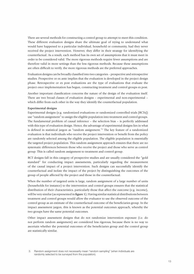
When the number of targeted units is large, random assignment of a large number of units (households for instance) to the intervention and control groups ensures that the statistical distribution of their characteristics, particularly those that affect the outcome (e.g. income), will be very similar (as represented in figure 1). Having similar statistical distributions between treatment and control groups would allow the evaluator to use the observed outcome of the control group as an estimate of the counterfactual outcome of the beneficiaries group. In the impact assessment jargon, this is known as the potential outcomes approach, whereby the two groups have the same potential outcomes.
Other impact assessment designs that do not randomize intervention exposure (i.e. do not perform random assignment) are considered less rigorous, because there is no way to ascertain whether the potential outcomes of the beneficiaries group and the control group are statistically similar.
3. Random assignment does not necessarily mean “random sampling” (when individuals are randomly selected to be surveyed from the population).
14
Non-experimental designsExperimental designs rely on randomization to create a counterfactual. If done properly, the analysis of the subsequent data is straightforward and statistical tests (such as the student’s t-test) can be used, since the treatment and control groups are alike in all ways except that the treatment group received the project.
In the non-experimental approach, the strategy is to use the best data possible and then apply statistical corrections as needed in order to account for the selection bias. Non-experimental designs often require stronger assumptions about the properties of the statistical parameters that cannot always be tested and can therefore be hard to defend. When designed ex ante as prospective impact assessments, their underlying assumptions are easier to defend if baseline data are available on both treatment and control groups. However, when designed ex post as retrospective impact assessments, their underlying assumptions are harder to defend.
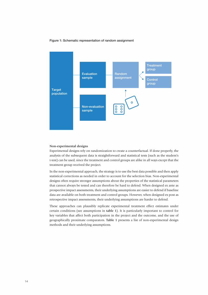
These approaches can plausibly replicate experimental treatment effect estimates under certain conditions (see assumptions in table 1). It is particularly important to control for key variables that affect both participation in the project and the outcome, and the use of geographically proximate comparators. Table 1 presents a list of non-experimental design methods and their underlying assumptions.
Figure 1: Schematic representation of random assignment
Target population
Evaluationsample
Random assignment
Treatmentgroup
Controlgroup
Non-evaluationsample
15
Table 1: Non-experimental designs and counterfactual validity: methodsFigure 1: Schematic representation of random assignment
Statistical methods Assumptions Requirements
Propensity score matching (PSM)
Conditional independence/unconfoundedness; sizable common support; similar external conditions facing treatment and control units
Requires only cross-sectional data.
Successful method if the evaluator knows the nature of possible selection biases.
Accounts for selection bias based on observables: in other words, observable characteristics are likely to affect project participation
The evaluator should have a clear understanding of targeting rules and individual take-up of the project.
Difference in Difference (DID) Relaxes conditional independence assumption or selection only based on observables
Requires panel data (4 samples: 2 for control group and 2 for treatment group at 2 different points in time).
Assumes that unobserved heterogeneity does not vary with time (hence it is time-invariant).
Parallel trend assumption: outcomes of treatment and control units follow the same path before the intervention
Method can be strengthened by combining it with propensity score matching (PSM) in order to also take into account selection on observables (DID+PSM).
Instrumental variable regression models
Selection based on unobservables is accounted for, provided that an “instrument” is found (e.g. a variable that is correlated with participation but not correlated with unobserved characteristics affecting the outcome y). Such variable is a determinant of the “assignment rule” or participation rule into treatment.
Cross-sectional or panel data.
Key requirements are to possess such “instruments,” have an a priori theory about them and include them in data collection.
“Make the unobservables observable.”
Regression discontinuity designs
Exogenous project rules (e.g. eligibility requirements) around a cut-off point.
Cross-sectional or panel data.
Requires clear targeting rules (e.g. smallholders with less than 3 hectares of land; beneficiaries selected based on credit risk scores; etc.).
Source: Garbero (2014b).
16
The importance of a careful design
As noted in the Information paper (IFAD, 2012a), mimicking randomization or reconstructing a valid counterfactual can be particularly challenging for agricultural projects, and thus ensuring attribution of the impact of the project on outcomes requires obtaining the best data possible and then using statistical methods to address remaining data issues. Generally, careful design and sampling can help to fortify both the internal and external validity of a study. Specifically, with regards to the validity of a study, there are two major issues to consider: 1. Internal validity: whether the measured impact is indeed caused by the project in
the sample; 2. External validity: whether the impact is generalizable to other samples or populations
(in other words, whether the results are generalizable and replicable).
In essence, the better the available data, the less complicated the required statistical procedures. Designing data collection for an impact assessment ex ante – that is, prior to project implementation – facilitates the process of creating a viable counterfactual and identifying a reasonable control group. On the other hand, designing impact assessments ex post – that is, doing data collection after implementation – is more challenging, as it requires the creation of a control group long after the targeting of beneficiaries has been performed at the beginning of the project, or even after the implementation of the project has ended. Identifying the control group ex post often means that neighbouring households and communities (the potential control group) are systematically different from beneficiaries (the treatment group), which can lead to “biased” estimates of the project impact.
The importance of taking a representative sample
Therefore, the design of the impact assessment has a very important influence on the extent to which causal claims can be made about the impact of a given project. The design of the survey instrument provides the universe of outcomes, while the sampling strategy determines the population for which the study is relevant. A representative sample is randomly sampled from some clearly defined population; as the size of the sample grows, the properties of the sample will converge on the correct population distributions.
Sampling will typically be driven by the targeting policies of the project. An evaluation of a pension project may never sample households without members over retirement age, or an agricultural inputs project might only study farming households. This is perfectly appropriate, but a researcher must be clear about the population that is relevant for the study, and then work carefully to design a sampling strategy that will correctly reflect this population.
The importance of the theory of change
Underlying the design of any impact assessment is a conceptual model that links the actions taken by the implementer to a set of intermediate outputs of the project, as well as to the ultimate impacts experienced by beneficiaries. At the core of the IFAD9 IAI is the concept of Theory-Based Impact Assessment. This concept is based around the following six principles (White 2009):
17
1. The initial step for a rigorous impact assessment is a clearly laid out theory of change (TOC), embedded in the project’s logical framework (logframe). The theory of change is defined as the causal chain that links project activities (inputs) to the results (outcomes and outputs) and impacts;
2. Understanding impact implies the need to know the context where the intervention took place. Essentially, this means understanding stakeholders’ needs and views regarding what the project is expected to deliver on the ground;
3. Understanding the context facilitates the evaluator’s capacity to anticipate the heterogeneity of the targeted population and the heterogeneity of impact. It is important to understand the level of heterogeneity of the population in terms of their characteristics (sex, age, proportion under the poverty line, etc.) and of the benefits/interventions they are receiving. The general rule is that the greater the heterogeneity, the larger the sample size needed;
4. A valid counterfactual should be established from the beginning of the project, i.e. the evaluation design needs to have a valid comparison/control group. In addition, in order to strengthen the design, panel data should be collected on both treatment and control groups. Hence, baselines should be designed in such a way as to allow re-identification of sample households;
5. A factual analysis should be undertaken using representative data prior to engaging in an impact assessment. This consists of a “targeting” analysis in which – provided that there is a defined target group – targeting errors and the characteristics of beneficiaries are assessed;
6. Mixed methods design should be part of the impact assessment strategy: qualitative research should be conducted to triangulate results of the quantitative component and respond to the “why” question.
Therefore, the first step in designing an impact assessment involves developing an explicit theory of change. In an ex ante or prospective framework, the question of “who will benefit from this project?” informs how the sample is selected. The question of “what are the expected benefits of the project?” informs which questions to ask in the baseline survey. The question of “what are the possible pathways for the benefit to take place” informs the study design and the selection of a control group (e.g. are the expected benefits taking place at the individual, community, or regional level?).
In an ex post or retrospective framework, developing the project’s theory of change is more challenging, as this implies reconstructing it ex post, or – in other words – a posteriori. Specifically with respect to the IFAD9 IAI, as noted in the information paper (IFAD 2012a), the indicators selected to assess the impact of a given IFAD-funded project and articulated in a logical framework should reflect the project’s specific theory of change, highlighting the impact pathway through which investments lead to results. The selected measures should be indicative of the specific objectives of that project and should vary depending on those. Of course, the objectives should also be consistent with the multiple objectives of the IFAD Strategic Framework.
18
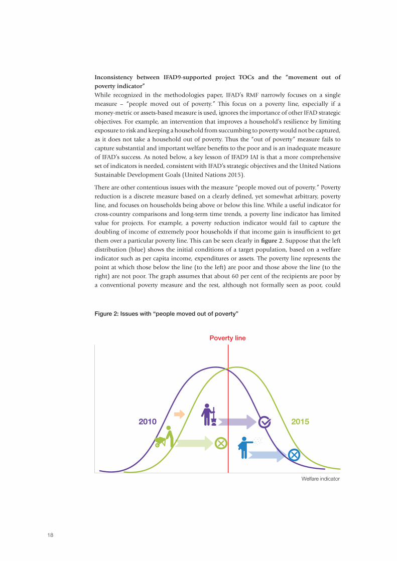
Inconsistency between IFAD9-supported project TOCs and the “movement out of poverty indicator”While recognized in the methodologies paper, IFAD’s RMF narrowly focuses on a single measure – “people moved out of poverty.” This focus on a poverty line, especially if a money-metric or assets-based measure is used, ignores the importance of other IFAD strategic objectives. For example, an intervention that improves a household’s resilience by limiting exposure to risk and keeping a household from succumbing to poverty would not be captured, as it does not take a household out of poverty. Thus the “out of poverty” measure fails to capture substantial and important welfare benefits to the poor and is an inadequate measure of IFAD’s success. As noted below, a key lesson of IFAD9 IAI is that a more comprehensive set of indicators is needed, consistent with IFAD’s strategic objectives and the United Nations Sustainable Development Goals (United Nations 2015).
There are other contentious issues with the measure “people moved out of poverty.” Poverty reduction is a discrete measure based on a clearly defined, yet somewhat arbitrary, poverty line, and focuses on households being above or below this line. While a useful indicator for cross-country comparisons and long-term time trends, a poverty line indicator has limited value for projects. For example, a poverty reduction indicator would fail to capture the doubling of income of extremely poor households if that income gain is insufficient to get them over a particular poverty line. This can be seen clearly in figure 2. Suppose that the left distribution (blue) shows the initial conditions of a target population, based on a welfare indicator such as per capita income, expenditures or assets. The poverty line represents the point at which those below the line (to the left) are poor and those above the line (to the right) are not poor. The graph assumes that about 60 per cent of the recipients are poor by a conventional poverty measure and the rest, although not formally seen as poor, could
Figure 2: Issues with “people moved out of poverty”
Welfare indicator
Poverty line
2010 2015
19
be viewed as vulnerable. Suppose the project shifts the beneficiaries’ welfare distribution (2010) in a positive direction to the welfare one in green (2015). This should be considered a successful project in that, on average, the beneficiary population is better off.
Now consider three farmers. The purple farmer is considered poor as he/she is below the poverty line. As indicated by the purple arrow, the project improves his/her well-being enough to move him/her above the poverty line and thus he/she is “moved out of poverty.” This would be counted in a poverty measure. The green farmer is very poor, with a much lower income than the purple farmer. The project increases his/her well-being dramatically as seen by the green arrow – an increase in welfare greater than the first farmer. Yet this has not moved him/her out of poverty, as he/she did not cross the poverty line. He/she does not count in a poverty reduction measure. The blue farmer is not considered poor by a conventional measure, but is clearly just getting by. As indicated by the blue arrow, the project helps him/her as well, but he/she is not considered poor prior to the project, so his/her gains are not counted as “moved out of poverty.” Clearly, the measure is flawed in that it fails to capture dramatic gains, as some farmers, even though they benefited from the project, did not cross an arbitrary poverty line. Hence, the “moved out of poverty” indicator is an inadequate measure of IFAD’s success.
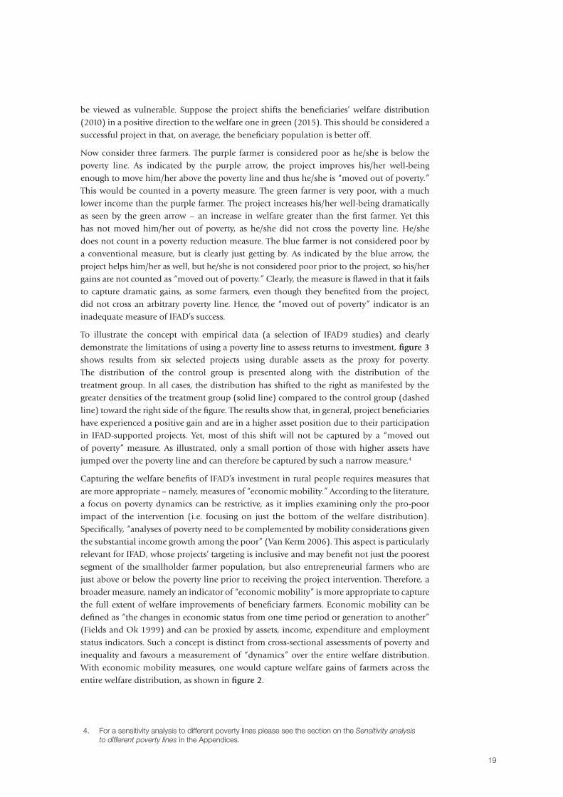
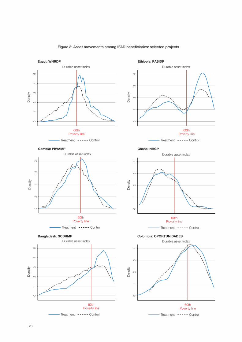
To illustrate the concept with empirical data (a selection of IFAD9 studies) and clearly demonstrate the limitations of using a poverty line to assess returns to investment, figure 3 shows results from six selected projects using durable assets as the proxy for poverty. The distribution of the control group is presented along with the distribution of the treatment group. In all cases, the distribution has shifted to the right as manifested by the greater densities of the treatment group (solid line) compared to the control group (dashed line) toward the right side of the figure. The results show that, in general, project beneficiaries have experienced a positive gain and are in a higher asset position due to their participation in IFAD-supported projects. Yet, most of this shift will not be captured by a “moved out of poverty” measure. As illustrated, only a small portion of those with higher assets have jumped over the poverty line and can therefore be captured by such a narrow measure.4
Capturing the welfare benefits of IFAD’s investment in rural people requires measures that are more appropriate – namely, measures of “economic mobility.” According to the literature, a focus on poverty dynamics can be restrictive, as it implies examining only the pro-poor impact of the intervention (i.e. focusing on just the bottom of the welfare distribution). Specifically, “analyses of poverty need to be complemented by mobility considerations given the substantial income growth among the poor” (Van Kerm 2006). This aspect is particularly relevant for IFAD, whose projects’ targeting is inclusive and may benefit not just the poorest segment of the smallholder farmer population, but also entrepreneurial farmers who are just above or below the poverty line prior to receiving the project intervention. Therefore, a broader measure, namely an indicator of “economic mobility” is more appropriate to capture the full extent of welfare improvements of beneficiary farmers. Economic mobility can be defined as “the changes in economic status from one time period or generation to another” (Fields and Ok 1999) and can be proxied by assets, income, expenditure and employment status indicators. Such a concept is distinct from cross-sectional assessments of poverty and inequality and favours a measurement of “dynamics” over the entire welfare distribution. With economic mobility measures, one would capture welfare gains of farmers across the entire welfare distribution, as shown in figure 2.
Figure 2: Issues with “people moved out of poverty”
4. For a sensitivity analysis to different poverty lines please see the section on the Sensitivity analysis to different poverty lines in the Appendices.
20
Figure 3: Asset movements among IFAD beneficiaries: selected projects
Den
sity
60thPoverty line
Durable asset index
01
23
45
ControlTreatment
Den
sity
60thPoverty line
Durable asset index
01
23
4
ControlTreatment
Egypt: WNRDP
Den
sity
60thPoverty line
Durable asset index
01
23
45
ControlTreatment
Bangladesh: SCBRMP
Ethiopia: PASIDP
Den
sity
60thPoverty line
Durable asset index
01
23
4
ControlTreatment
Ghana: NRGP
Den
sity
60thPoverty line
Durable asset index
0.5
11.
52
ControlTreatment
Gambia: PIWAMP
Den
sity
60thPoverty line
Durable asset index
01
23
4
ControlTreatment
Colombia: OPORTUNIDADES
21
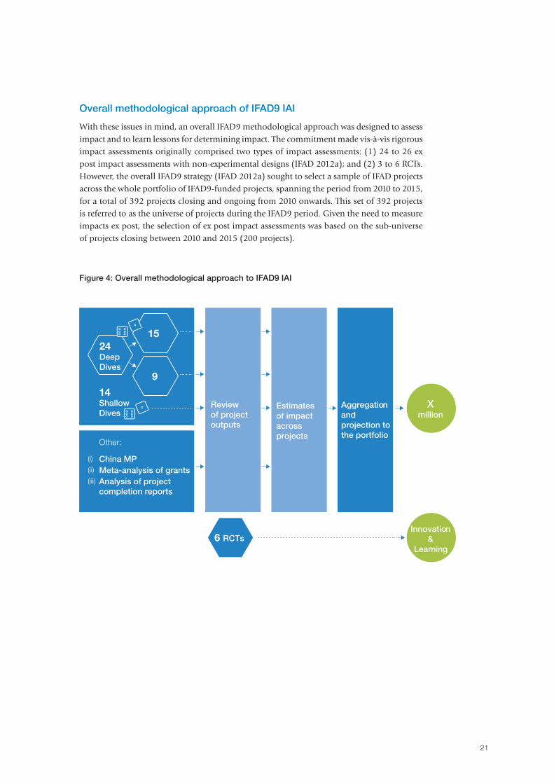
Figure 4: Overall methodological approach to IFAD9 IAI
Overall methodological approach of IFAD9 IAI
With these issues in mind, an overall IFAD9 methodological approach was designed to assess impact and to learn lessons for determining impact. The commitment made vis-à-vis rigorous impact assessments originally comprised two types of impact assessments: (1) 24 to 26 ex post impact assessments with non-experimental designs (IFAD 2012a); and (2) 3 to 6 RCTs. However, the overall IFAD9 strategy (IFAD 2012a) sought to select a sample of IFAD projects across the whole portfolio of IFAD9-funded projects, spanning the period from 2010 to 2015, for a total of 392 projects closing and ongoing from 2010 onwards. This set of 392 projects is referred to as the universe of projects during the IFAD9 period. Given the need to measure impacts ex post, the selection of ex post impact assessments was based on the sub-universe of projects closing between 2010 and 2015 (200 projects).
24 Deep Dives
6 RCTs
14 Shallow Dives
Review of project outputs
Other:
China MPMeta-analysis of grantsAnalysis of projectcompletion reports
(i)
(ii)
(iii)
Estimatesof impactacrossprojects
Aggregationand projection to the portfolio
15
9
Xmillion
Innovation&
Learning
22
Therefore, the selection strategy for the ex post assessments sought to serve two objectives. First, projects had to be suitable for an ex post impact assessment with the overarching aim of measuring the poverty reduction impact and, second, such projects had to be statistically representative of the portfolio of activities undertaken by IFAD during IFAD9. The estimated impacts calculated for such a sample would have to be extrapolated; in other words, the estimated impact would have to be projected to the entire universe (392 projects during the IFAD9 period).
While the selection of the RCTs had to be conducted on an ad hoc basis in order to meet the geographical and thematic criteria specified by the Funders5 – the Bill & Melinda Gates Foundation, and the United Kingdom’s Department for International Development (DFID) – the 24-26 ex post evaluations were selected based on a rigorous process with a view to extrapolating their results to the rest of the IFAD9 portfolio of projects. Thus, a statistical inventory of all IFAD9 projects with baseline, midline, or completion survey datasets (about 133 datasets) was conducted to establish the sub-universe of projects with datasets (around 122 projects out of 200 at the time of producing the inventory in June 2013) and their data quality.
The outcome of this work led to the production of an Inventory Report (Garbero and Pacillo 2013), a document clearly highlighting the limitations of the data. Projects with datasets were then ranked by region, based on data quality indexes, in order to provide an indication of data reliability (real versus fraudulent responses, verification of sampling design, presence of missing data, and out-of-range observations). A representative sample of projects to be evaluated was then determined by drawing a stratified random sample (a total of 41 projects, i.e. 26 first-choices and 15 reserves) from the universe of projects (with available datasets) closing between 2010 and 2015. Given two important criteria to be met – the evolution of the IFAD9 portfolio towards fewer projects and larger outreach numbers, and the need to capture the poverty reduction impact – an oversampling strategy was devised in order to make sure that the sample was representative of such features. Hence, two strata were defined: one group with mean outreach estimates and a baseline poverty head count above the regional median, and a second group with estimates of outreach and baseline poverty head counts below the regional median. In essence, projects in the former strata were oversampled by region in order to have a large enough sample of projects with large outreach estimates and higher poverty rates at baseline.
An internal consultation with IFAD Regional Directors and divisional representatives was then conducted to endorse the list of randomly selected projects to be evaluated by the external research partners. This process led to the replacement of 11 randomly selected projects with a set of purposively selected ones (purposive evaluations), given their strategic relevance and overall performance across the portfolio. Two of the purposively selected projects were dropped (namely, those in India and Senegal) after discussing the feasibility with internal staff.
In order to maintain the integrity of the representative sample, IFAD decided to maintain the randomly selected projects excluded from the final list of ex post evaluations and conduct the ex post assessments in-house using secondary (observational) data. This led to the genesis of the “Shallow Dives,” a term that allowed the Fund to distinguish such evaluations from the “Deep Dives”, the ex post evaluations that were conducted in partnership with research centres and that foresaw primary data collection. The Shallow Dives are ex post evaluations
5. For further details, see the section on the Experimental designs (RCTs) under the 3ie Agricultural Innovation Window in the Appendices.
23
that employ secondary data and non-experimental methods applied to existing surveys.
An analysis was conducted on a total of 14 randomly selected projects that were not included
among “Deep Dives”, along with the projects that were selected as Deep Dives reserves.
Note that Shallow Dives studies only complement the Deep Dives in answering the narrower
accountability question, that is, they only provide numerical estimates of the number of
beneficiaries moved out of poverty and estimates of economic mobility.
Rigorous retrospective (or ex post) impact assessments (24-26 Deep Dives)The 24-26 ex post studies are retrospective studies, i.e. project-level evaluations conducted
either at the time of completion or after the project closed. Only non-experimental designs
were employed for these studies, with specific methodologies that determine the impact in
the absence of a control group from an experimental design, and allow one to understand
the causal chain and measure attribution to IFAD. These non-experimental methods create
a counterfactual using statistical procedures. Recall that counterfactuals are needed to assess
the likely impact of an intervention (i.e. the “treatment” under analysis). The intention is to
ensure that the characteristics of the treatment and comparison groups are identical in all
respects, other than the intervention, as would be the case for an experimental design.
These studies were fully funded by IFAD. The commitment clearly specified that they had to
be conducted in partnership with a diverse set of external research centres (listed in table 3).
Thus, a number of research centres, with comparative advantages both in terms of data
collection and impact assessment expertise in the regions of interest, were contacted. Primary
data collection was conducted for the majority of the impact assessments, conditional on
the research partners’ cost structure and specificity of the study. Initially, these studies were
conceived as having a mixed-method research design, with the main focus being on the
quantitative surveys. However, qualitative surveys were also included as part of the impact
assessments, conditional on the specific budgetary constraints of research partners. The benefit
of conducting focused qualitative studies is that their findings can provide detailed data on
the local context and help contextualize the impact findings from the quantitative analysis.
With the aim of moving beyond the poverty indicators, and moving towards analysing
the entire income distribution of the targeted population, the overarching evaluation
focus became both an assessment of economic mobility (defined as changes in “economic
well-being” of beneficiary farmers), determined through asset-based measures, and an
assessment of poverty dynamics (defined as the number of beneficiaries that have been moved
out of poverty). These impact assessments also attempted to report on the contribution of
IFAD’s interventions towards women’s empowerment, economic resilience, adaptive capacity
and nutritional outcomes, whenever these outcomes were relevant within the project-specific
theory of change.
In addition, the IFAD9 IAI sought to provide evidence on broader aspects related to the
impact of an IFAD-supported project in a country-specific context. Ideally, findings were
expected to help close the current evidence gap affecting similar types of project activities
or interventions. Some of the lessons learned were also meant to provide insights around
programmatic arrangements and empirical conditions that are needed to conduct more
comprehensive evaluations that produce more accurate estimates of impact. Details on
the impact assessment framework can be found in the section on the IFAD9 ex post impact
assessments: overview of evaluation framework in the Appendices.
24
China multiple-projects study (China MP – phase II of the “econometric study”) Aside from the impact assessments of 24-26 IFAD projects, the methodology paper included
an additional set of ex post impact assessments, with the objective to provide an analysis
of the impact of seven IFAD projects in China (closing between 2010 and 2015) using
retrospective cross-sectional data in a cumulative manner (IFAD 2012a). This is an update
of an econometric study originally conducted in 2011 by the School of Economics and
Management at the China University of Geosciences (Shuai et al. 2011). This study examined
the following six impact dimensions: household income and assets, human and social
capital and empowerment, food security and agricultural productivity, natural resources and
environment, institutions and policies, and sustainability. The results from this study are
noted in table 3 and are included in the aggregate impact estimates.6
Summary of studies undertaken under IFAD9The final number of ex post impact assessments is presented in table 3. Of the 37 ex post
impact assessments, some were randomly selected (15 Deep and 14 Shallow Dives) and
10 others were purposively selected (9 Deep Dives and 1 China MP), owing to different
constraints (political and practical). Moreover, two of the 24 Deep Dives were not completed
on time (in Kenya and Madagascar), and were thus excluded from the analysis. Lastly, two ex
post assessments were merged into one study (PRISM and MIOP projects in Pakistan), hence
the total number of impact assessments listed in table 3 amounts to 36 studies.
All projects listed in table 3 were reviewed to determine outputs. Impact on relevant indicators
was then assessed using non-experimental methods appropriate for the specific ex post data
collection. Unfortunately, the available project data even for these projects were inadequate
for proper impact assessment, requiring primary data collection in a number of cases and,
where possible, collection of secondary data from sources other than IFAD. Although the
Deep Dives were analysed by external teams, the results were systematically replicated by
IFAD staff members to ensure accuracy and consistency, and also to remove analyst bias
in view of the aggregation and projection exercises. The next section describes the IFAD9
methodology and estimation strategy in detail.
IFAD9 ex post IA’s studies, methodology and estimation strategy
The IFAD9 IAI Sourcebook (Garbero 2014b) is a document that was developed at the beginning
of the IFAD9 IAI to guide participating institutions on key methodological aspects related
to the IFAD9 IAI and, more specifically, on how to conduct rigorous impact assessments.
An overall evaluation framework was developed by staff members within IFAD, along with
technical guidance related to research design, including sampling and identification strategy,
indicator construction and questionnaire development. Two sets of questionnaires (a short
and long form, conditional on the budget of the external research partners) were developed
to make sure that the participating institutions would collect the same information at impact
and outcome levels, and, more specifically, the same indicators in view of the aggregation.
The following section describes the methodological choices that were recommended.
Study external validity and sampling strategyExternal validity means that the impact estimated for the impact assessment sample can
be generalized to the population of all eligible units. For this to be possible, the sample
must be representative of the population of eligible units. In practice, it means that the
sample must be selected from the population by using one of the several variations of
6. This document refers to this study either as “China Multiple” or China MP.
25
random sampling methods. Therefore, the sampling strategy is the most important factor
in any impact assessment exercise, as it allows the identification of project impact and also
analyses the heterogeneity of impact among the various actors. In the IFAD9 IAI selected
studies, heterogeneity of impact is a common factor. Different types of interventions can have
varied impacts on different types of smallholders, and the evaluator would need to identify
and measure these heterogeneous outcomes separately. To achieve this, and with a view to
capturing the poverty impact of the project, a stratified random sample was recommended in
order to ensure representativeness within the different groups of the population (strata), i.e.
by income groups or any other proxy for welfare. In order to have valid inference from each
of these subgroups, stratification was encouraged when possible.
Second, given the limitation of existing monitoring data – largely the absence of systematic
databases of beneficiaries, particularly due to the long gestation of IFAD-supported projects
(with average project life spanning 7.5 years) and to the inherent limitations of ex post
evaluations – a beneficiaries enumeration exercise or listing was recommended in order to
establish the sampling frame.
Third, an oversampling strategy of analytical domains, such as the “transient” poor or those
around the poverty line, was also recommended in order to capture the poverty mobility of
the targeted population.
Forth, village-level matching was recommended for selecting comparison villages (ex post)
with similar characteristics (pre-intervention) before drawing the household-level sample.
Fifth, power calculations anchored to poverty outcomes (using per capita expenditures, for
instance) were recommended to determine the size of the treatment and control group under
an ideal balanced experimental design. In addition, the ideal sample size had to be increased
proportionally (ideally by a factor that is calculated by dividing the sample size by a proportion
that the evaluator expects to have left after trimming the sample to the common support,
while using non-experimental designs such as propensity score matching). Where not enough
information was known about the characteristics of the treatment group in advance, or where
it was not possible to target the comparison group very precisely, it was recommended to
increase the comparison group up to ten times the size of the treatment sample. However, if
sufficient information was known about the treatment group, a comparison group sample
20 per cent larger than the treatment sample was considered adequate.
Study internal validityInternal validity means that the estimated impact of the project is net of all other potential
confounding factors, or that the comparison group represents the true counterfactual, so that
one can estimate the true impact of the project. In an earlier section, this paper highlighted
how random assignment produces a comparison group that is statistically equivalent to the
treatment group at baseline, before the programme starts. In all the ex post IFAD9 IAI selected
studies, the assignment was non-random and this was due to: (1) beneficiaries’ self-selection
into the project; and (2) the selection mechanism of the agency (whether IFAD or the local
implementers) managing the project. Self-selection refers to a farmer’s choice to participate
in the project. The agency selection mechanism is based on targeting rules, as implementers
decided to give the projects to those more in need. As long as the factors that drive selection
are known, one can estimate the causal impact of the project. However, the factors that drive
the selection mechanism can have an observable and unobservable nature. Unobservable
26
factors can be either due to lack of information or missing data (contingent unobservables), or be genuinely unobservable (hidden unobservables), such as entrepreneurial or innate ability, propensity to bear risks, ethical attitudes and so forth. These aspects are difficult to measure even with carefully designed indicators. Another key difficulty with the IFAD9 IAI was that, in some instances, the targeting mechanism was not exact from the analyst’s perspective or, in other words, there was no perfect compliance. As a result, no measure could perfectly predict project participation, and thus certain communities or villages might have received treatment, while others that might be similar did not receive treatment.
Cognizant of these empirical challenges, the estimation strategy of treatment effects, or equivalently, the estimation strategy to estimate the causal impact of the project had to rely on methods that are capable of identifying the causal parameters even in the presence of non-random assignment of project interventions to beneficiaries and non-beneficiaries. Such methods are able to mimic the counterfactual framework statistically.
Specifically, five approaches were used for the analyses of both Deep and Shallow Dives.7
These approaches estimated average treatment effects (ATEs) under the assumption of selection on observables. Selection on observables implies that all the relevant information about the true non-random selection-into-treatment process, which produces the observed sets of treated and untreated observations, is known to the analyst. Hence, by assumption, any possible presence of hidden unobservable characteristics is ruled out or considered to be minimal. This choice was made on the grounds that, in the data collection, researchers were encouraged to address the issue of contingent unobservables, prior to fielding the survey (the principle of “making unobservables observables”). This was done through a risk aversion module that was meant to capture farmers’ hidden preferences, ability and attitudes.
IFAD9 IAI estimation strategy The analyses of Deep Dives and Shallow Dives involved the estimation of treatment effects from observed data. Recall that a treatment effect is the change in an outcome caused by an individual getting the treatment instead of another. For the reason explained in the section on a precise definition of the counterfactual, one cannot estimate individual-level treatment effects because the outcome of each individual is only observable in one state: either receiving a treatment or receiving no treatment.
The potential outcome models, as mentioned previously, provide a solution to this missing data problem and allow a researcher to estimate the distribution of individual-level treatment effects. In this section, the discussion delves into the detailed econometrics behind the estimation strategy.
A potential outcome model specifies the potential outcomes that each individual would obtain under each treatment level, the treatment assignment process and the dependence of the potential outcomes on the treatment assignment process. When the potential outcomes do not depend on the treatment levels, after conditioning on covariates, regression estimators, inverse-probability-weighted estimators and matching estimators are commonly used. The term potential outcome model is equivalent to the Rubin causal model and the counterfactual model.8
7. Note that the IFAD9 IAI analyses used approaches similar to those of the Independent Office of Evaluation of IFAD in their two impact assessment studies.
8. See Rubin (1974); Holland (1986); Robins (1986); Heckman (1997); Heckman and Navarro-Lozano (2004); Imbens (2004); Cameron and Trivedi (2005); Imbens and Wooldridge (2009); and Wooldridge (2010) for more detailed discussions.
27
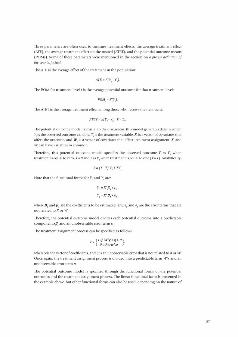
Three parameters are often used to measure treatment effects: the average treatment effect (ATE), the average treatment effect on the treated (ATET), and the potential outcome means (POMs). Some of these parameters were mentioned in the section on a precise definition of
the counterfactual.
The ATE is the average effect of the treatment in the population:
ATE = E(Y1 - Y0).
The POM for treatment level t is the average potential outcome for that treatment level:
POMt = E(Yt).
The ATET is the average treatment effect among those who receive the treatment:
ATET = E(Y1 - Y0 | T = 1).
The potential outcome model is crucial to the discussion: this model generates data in which Yi is the observed outcome variable, Ti is the treatment variable, Xi is a vector of covariates that affect the outcome, and Wi is a vector of covariates that affect treatment assignment. Xi and Wi can have variables in common.
Therefore, this potential outcome model specifies the observed outcome Y as Y0 when treatment is equal to zero, T = 0 and Y as Y1 when treatment is equal to one (T = 1). Analytically:
Y = (1 - T) Y0 + TY1.
Note that the functional forms for Y0 and Y1 are:
Y0 = X’ β0 + ϵ0 ,
Y1 = X’ β1 + ϵ1 ,
where β0 and β1 are the coefficients to be estimated, and ϵ0 and ϵ1 are the error terms that are not related to X or W.
Therefore, the potential outcome model divides each potential outcome into a predictable component xβt and an unobservable error term ϵt.
The treatment assignment process can be specified as follows:
where γ is the vector of coefficients, and η is an unobservable error that is not related to X or W. Once again, the treatment assignment process is divided into a predictable term W’γ and an unobservable error term η.
The potential outcome model is specified through the functional forms of the potential outcomes and the treatment assignment process. The linear functional form is presented in the example above, but other functional forms can also be used, depending on the nature of
0 otherwiseT = ,
28
the outcome. In the remainder of this section, the set of functional forms for the potential
outcomes is referred to as the outcome model, and the treatment assignment process is
referred to as the treatment model.
Three key assumptions underpin the different treatment effect estimators in question,
namely: (1) the conditional independence (CI) assumption, which restricts the dependence
between the treatment model and the potential outcomes given the covariates; (2) the
overlap assumption, which ensures that each individual could receive any treatment level;
and (3) the independent and identically distributed (i.i.d.) sampling assumption, which
ensures that the potential outcomes and the treatment status of each individual are unrelated
to the potential outcomes and treatment statuses of all other individuals in the population.
This third assumption is what is known as SUTVA, the stable unit treatment value assumption
(Imbens and Woolridge 2009; Woolridge 2010). Note that these assumptions may vary
across estimators. The SUTVA assumption states that the observed differences in outcomes
between treatment and control units only depend on one’s own treatment status, and not the
treatment status of the other units.
The following five econometric methods were used to provide correct inference for causal
parameters, specifically: (1) regression-adjustment (RA); (2) propensity score matching
(PSM); (3) covariate matching (NN or NNM);9 (4) inverse-probability weighting (IPW); and
(5) the doubly robust estimator (IPWRA).
Regression adjustment (RA)RA is the base-case estimator, which uses the mean of the predicted outcomes for each
treatment level to estimate each POM. ATEs and ATETs are differences in estimated POMs.
RA estimators model the outcome without any assumptions about the functional form for
the probability of the treatment model.
Two matching estimatorsMatching estimators use the average of the outcomes of the nearest individuals to impute the
missing potential outcome for each sampled individual. The difference between the observed
outcome and the imputed potential outcome is an estimate of the individual-level treatment
effect. These estimated individual-level treatment effects are averaged to estimate the ATE or
the ATET.
Propensity score matching estimatorsOne type of matching is propensity score matching, where the nearest neighbour in the
control group can be determined by using the estimated treatment probabilities based on the
selected covariates, which are known as the propensity scores. Also, instead of performing
bias correction to handle the case of more than one continuous covariate, a la Abadie (2011),
a common solution is to combine all the covariate information into an estimated propensity
score and use this single continuous covariate as the matching variable. The PSM estimator
parameterizes the bias-correction term in the treatment probability model (Rosenbaum
and Rubin 1983). Corrected standard errors were estimated using the Abadie and Imbens
(2012) method.
Covariate matching estimatorsWithin matching estimators, covariate matching is employed, where the nearest neighbour
in the control group is identified by using a weighted function of the covariates for each
treated observation. This type of matching is known as nearest-neighbour matching (NNM).
9. Both (2) and (3) are matching estimators.
29
NNM is non-parametric, as no functional form is needed either for the outcome model or the treatment model. When matching on more than one continuous covariate, this can introduce bias to the matching estimate. Abadie and Imbens (2006, 2011) have provided a bias correction for this matching estimator, which is implemented in the estimation strategy.
Inverse-probability-weighted (IPW) estimatorsIPW estimator uses weighted averages of the observed outcome variable to estimate means of the potential outcomes. The weights account for the missing data inherent in the potential-outcome framework. Each weight is the inverse of the estimated probability that an individual receives a treatment level. Outcomes of individuals who are more likely to get treatment are assigned a weight close to one. Outcomes of individuals who are less likely to get treatment are assigned a weight larger than one, potentially much larger. IPW estimators model the probability of treatment without any assumptions about the functional form for the outcome model.
Inverse-probability-weighted regression-adjustment (IPWRA) estimatorsIPWRA, also known as “Wooldridge’s doubly-robust” estimator because it was derived by Wooldridge (2007), is discussed at length in Wooldridge (2010). It models both the outcome and the treatment probability, and has the property of being doubly robust, which means that only one of the two models must be correctly specified to consistently estimate the treatment effects. In summary, the IPWRA estimator uses the inverse of the estimated treatment-probability weights to estimate missing-data-corrected regression coefficients that are subsequently used to compute the POMs.
Instead of using a single estimator, the results obtained from the five different estimators presented above were compared. Note that all externally conducted Deep Dives were replicated in-house to allow one to have identical estimation strategies. Variable constructions in the Shallow Dive studies were also conducted in-house by IFAD.
There are different perspectives regarding the choice of the estimators. Rosenbaum and Rubin (1983) first showed that balancing two samples on the propensity score can equalize their observable covariate distributions for the purposes of programme evaluation. Several similar estimators have been shown to be unbiased; however, there is disagreement in the literature about which methods are the most efficient. Abadie and Imbens (2006) show that a covariate matching estimator is root-N consistent and asymptotically normal under certain conditions, and Hirano, Imbens and Ridder (2003) show that a propensity score weighting estimator is asymptotically efficient relative to other propensity score estimators. More recently, Busso, DiNardo and McCrary (2013) show that among propensity score matching, covariate matching and propensity score reweighting estimators, covariate matching estimators perform best with a small number of average matches when overlap is poor between the treatment and control groups, whereas propensity score weighting with normalized weights performs best when overlap is substantial. Huber, Lechner and Wunsch (2010) perform a larger Monte Carlo simulation and find that bias-adjusted radius matching is preferable, particularly when the propensity score is mis-specified. They claim that the difference is potentially due to the difference between the small samples used by Busso, DiNardo and McCrary (2013) and, earlier, by Fröhlich (2004). However, as discussed by Abadie and Imbens (2006), it is not clear how to perform statistical inference for propensity score matching estimators, as analytical estimates are incorrect and the validity of bootstrapped standard errors is unclear.
30
More recently, Imai and Ratkovic (2014) have suggested a method for estimating covariate
balanced propensity scores, which simultaneously chooses variables that balance covariates
between the treatment and control groups, and then estimates propensity scores. They argue
that this method improves the performance of both propensity score matching and
weighting estimators.
Prior to choosing the exact covariates that could enter the various estimators, IFAD IAI
analysts decided to remain sceptical about the optimal matching covariates, and ran the
Imai and Ratkovic (2014) covariate balancing propensity score (CBPS) method to model
treatment assignment while optimizing the covariate balance. This method approximates a
non-parametric relationship between the treatment indicator and the explanatory variables,
and leaves the analyst agnostic to the variables that are included in the propensity score
construction. The same covariates are then used in both the reweighting estimators described
above and the matching estimators.
Note that the following covariates were included as likely to be unaffected by treatment and
used for matching:
• Invariant household characteristics such as age and gender of household head; education
level of household head; household size or composition, etc.
• Village-level covariates such as area, population, calculated village averages, distance to
the nearest markets or roads
• Geographical indicators such as altitude and precipitation
• Recall values for household durables, farm and livestock assets, where reasonable
• Previous exposures to shocks, where appropriate
• Interaction and higher-order terms of some variables were introduced to allow for
non-linearity.
The final specification was based on model performance using evidence for sufficient overlap,
common support, and bias reduction between treatment and control groups, as indicated by
the suggested criteria in the literature (B<25%, R~1). B, the Rosenbaum and Rubin’s bias,
can be defined as the number of standard deviations between the means of the covariates
in the treatment and the control groups. R can be defined as the ratio of the variances of the
covariates in the treatment and the control groups (Rubin 2001).
Additionally, to test for the sensitivity of the estimated treatment effects, Rosenbaum
bounds were also calculated on the estimates. The Rosenbaum bounds test whether the
treatment effects obtained are driven by the hidden bias due to unobservable characteristics.
By gradually increasing the magnitude of hidden bias at various increments, the Rosenbaum
bounds report which level of hidden bias would drive the estimated treatment effects
(Rosenbaum 2002).
Intention to treat (ITT)It is worth stressing that IFAD9 studies were plagued by a methodological issue, namely imperfect
compliance. This term substantially indicates the case where the treatment group does not get
the treatment as intended, or when the control group gets some treatment as unintended.
When this occurs, the results obtained are considered to be the intention to treat (ITT) effects.
This estimate is still robust because: (a) it is conservative (it underestimates the full potential
of an intervention in case of imperfect compliance); and (b) it is less prone to selection bias.
In such cases, the causal effect of assignment to the treatment group and not necessarily the
treatment itself is evaluated. In ITT, T = 1 if the individual farmer (or village for instance)
is assigned to the treatment group (irrespective of whether or not the actual treatment is
received/adopted by the farmer), and T = 0 if an individual is assigned to the control group
(irrespective of whether the farmer opted in the intervention, e.g. decided to buy seeds with
his/her own money, instead of remaining untreated in the control group). Therefore, in the
face of imperfect compliance, the ITT effect will underestimate the true causal effects, as
E(Y1i | Ti = 1) will be underestimated and E(Y0i | Ti = 0) will be overestimated.
In conclusion, the analysis of the Deep Dives used cross-sectional data and the econometric
methods described above to identify impact and ensure robustness. The robustness of results
was assessed by estimating project impacts with several models of single-difference on the
matched observations.
The Shallow Dives were analysed by IFAD using synthetic-panel techniques on secondary
data combined with the above-mentioned econometric methods. Given the main focus of
Shallow Dives on having to estimate dynamics of poverty and economic mobility from existing
surveys, only these estimates were produced. The Shallow Dives methodology is illustrated
in a companion paper (Garbero 2014a) where the author produced estimates of poverty
dynamics and economic mobility estimates in the absence of panel data, money-metric
indicators and comparison groups, for a Vietnamese IFAD-supported project. Besides being
data-intensive, a number of assumptions had to be verified empirically for the validity of
the method to hold (for more details, see Garbero 2014a). This methodology essentially
combines the use of synthetic panels (Dang et al. 2014), namely the non-parametric bounding
approach, with non-experimental methods applied to asset-based composite indices. For a
full set of results on the Shallow Dives, see a forthcoming paper (Garbero, Brailovskaya,
and Giera 2016). The final results are estimates of the average effect of the projects on given
indicators when the treatment group is compared with the control group.
Estimation strategy for the poverty dynamics and economic mobility proxy indicators
Another crucial methodological aspect around the IFAD9 IAI revolved around the choice
(and the estimation methodology) of the welfare proxies, poverty and economic mobility
outcome, as well as the choice of poverty lines.
The information paper Methodologies for Impact Assessments for IFAD9 highlights that “measuring
and comparing income-poverty is notoriously complex, but in view of the need for comparison and
aggregation, an income-based definition of poverty is useful” (IFAD 2012a). However, recognizing
the difficulty of such a measure further notes that income-level equivalents of poverty proxies
could be acceptable, namely asset-based indicators. While income data were collected in a
few studies, the data were insufficient and did not lend themselves to the computation of
poverty dynamics.
The IFAD9 IAI has thus relied on asset-based indicators as proxy indicators for the poverty
and economic mobility outcomes. Although money-metric indicators are considered
superior welfare indicators, asset indices have been used widely in the literature as proxies
for wealth (Howe et al. 2009), long-run economic status (Filmer and Pritchett 2001) or
household welfare (Wall and Johnston 2008). Hence, the rationale for undertaking poverty
and economic mobility analyses based on asset indices is largely justified.
31
32
In essence, low asset index scores tend to correspond to low levels of long-run wealth/welfare/economic status; they have been found to constitute robust predictors of a range of other outcomes, most notably in the health and education domains across a variety of contexts (Filmer and Scott 2012).
However, while asset indices are widely used for cross-sectional poverty assessments, the relevant literature has highlighted their drawbacks in terms of being able to capture poverty dynamics (Booysen et al. 2008; Sahn and Stifel 2000). Asset-based indicators are essentially slow-moving and may lead to a potential underestimation of impact of IFAD-funded projects (Booysen et al. 2008). The core issue is the slow rate of change in the underlying asset variables. It is thus possible that changes may take place in the economic situation of many households while asset indices remain virtually unaltered. Therefore, the authors caution against using asset indices to understand short- or medium-term economic mobility, or variability in household welfare. In addition, asset indices do not discriminate well at the lower end of the welfare distribution, which makes the index inappropriate for analysing ultra-poverty (Booysen et al. 2008). It is worth noting that these issues are less of a concern in the context of IFAD-supported projects, as the phenomenon of interest is long-term poverty reduction and changes in economic mobility across the project life (the average duration of IFAD-supported projects being about 7.5 years).10
In relation to poverty lines, and given that poverty will be proxied by asset indicators, the literature performing inter-temporal poverty comparisons using asset-based indicators (Booysen et al. 2008) has suggested the use of two poverty lines – the 40th and the 60th percentile of the baseline distribution. Going along with this recommendation, the poverty lines are also set at the 40th and 60th percentiles of the durable asset index baseline distribution for the IFAD9 IAI studies. In addition, the 60th percentile is adopted as the preferred poverty line specification for at least two main reasons. First, the durable asset index better approximates long-run wealth (Filmer and Pritchett 2001); second, based on a descriptive analysis of baseline asset index distributions using available RIMS data, the bulk of IFAD beneficiaries were found to be below the 60th percentile cut-off, particularly in the second and third quintiles. Furthermore, when comparing baseline and endline distributions using the same data, upward shifts in economic mobility were more likely to be observed at the 60th percentile cut-off of the country-specific baseline asset index distribution. Therefore, the poverty threshold set at the 60th percentile cut-off is deemed the most appropriate.
Alternatively, poverty lines could be set at the index value yielding the same prevalence of poverty as that yielded by the international poverty lines (US$1.25/US$2/US$2.50 per day lines) or national poverty lines, applied to total expenditures or income measures. Note that these options can only be computed with datasets that include both expenditure or income and assets.11 Given that only a handful of IFAD9 studies contained both money-metric and asset-based measures, a sensitivity analysis was conducted on a selected number of IFAD9 studies to verify poverty classifications obtained through relative versus absolute (both national and international) poverty lines (see the section on the Sensitivity analysis to
different poverty lines in the Appendices for these results).
Turning to the actual estimation strategy of the asset indices used as part of IFAD9 IAI, a number of asset indices were constructed in order to better characterize farmers’ relative wealth. The literature (Filmer and Pritchett 2001) defines an asset index as any composite indicator where the underlying variables on which it is based reflect a household’s ownership
10. In addition, targeting is generally directed towards smallholder farmers around the poverty line and not necessarily the ultra-poor.
11. This option is only possible in an ex post impact assessment collecting primary data.
33
(or lack thereof) of a range of assets. Thus, the asset index is a function of these variables,
assets aij, where aij denotes household i’s ownership of asset j,
Ai = f(ai1) = f(ai1,,…,aim).
The simplest way to compute an asset index is by a simple count of the assets j = 1,…,m that
households i = 1,…,n own, i.e.
Ai = ai1 + ai2 + … + aim = 1 if household i owns asset j, and aij = 0 otherwise.
There are three factors that are crucial for the determination of an asset index: the choice
of assets that enter the construction of the index, how ownership (or lack thereof) of assets
j = 1,…,m translates into values of the respective variables and the methodology to construct
the composite index Ai.
The methodology is indeed the most important aspect that determines the structure of an
asset index. In theory, any function of aij can be deemed an asset index. In the literature,
the dominant approach is for Ai to be computed as a linear combination of the underlying
variables aij, that is,
Ai = vi1 xai1 + vi2 xai2 + … + vim xaim ,
where vij are the weights assigned to the underlying asset variables ai1.
If the index is a simple asset count, arbitrary weights can be assigned to each of those
variables. However, two methodologies have gained prominence in the literature, whereby
weights are assigned based on the variance and covariance of the asset variables aij themselves
– whether through factor analysis (FA), principal components analysis (PCA) or multiple
correspondence analysis (MCA). These are data reduction techniques that aim at uncovering
the underlying structures in datasets (called factors in FA and components in PCA and MCA),
computed through transformations of the datasets themselves. The output of PCA, MCA and
FA is a set of factors or components that are at most equal in number to the original variables,
but in standard practice only the first of these (the one that accounts for the largest share of
the variance-covariance in the dataset) is used to compute the asset index.
In the context of these methodologies, the objective is to uncover the underlying pattern of
asset ownership across the sample of households. Weights are data-driven and act as the vector
of coefficients that transform the original matrix of asset variables aij into the first principal
component (PCA, MCA) or into the most important latent factor (FA). The relevant literature
has also interpreted the underlying pattern differently: some as a wealth gradient (Howe et
al. 2009; Howe et al. 2012), others as long-run economic status (Filmer and Pritchett 2001)
or household welfare (Wall and Johnston 2008), where low asset index scores are assumed
to correspond to low levels of long-run wealth/welfare/economic status. This should be
reflected in the pattern of asset ownership across the sample as the main unobserved variable
underlying that dataset. The literature has also shown that asset indexes are robust predictors
of health and education outcomes, across a variety of contexts (Filmer and Scott 2012).
Note that in the IFAD9 analyses, the underlying variable is defined as an index of relative
long-run wealth.

34
MCA was employed to compute a household asset index based on durable items. The following items were included in the computation of the index: housing characteristics (roof material, floor material, wall material, number of rooms per capita, toilet facilities, kitchen facilities, source of water, source of cooking fuel, whether the household had electricity), and durable assets such as motorbike, bicycle, car, stove, TV, radio, mobile phones.
In addition, the following steps were undertaken to obtain a statistically valid index:
1. Variables with no or insufficient variation were dropped;
2. Value labels were re-coded in an increasing ordinal scale (where the lowest value was the “no-asset” level) in order to make them consistent with the First Axis Ordering Consistency (FAOC-I) property – that is, in order to ensure an ordinal consistency between the ordering of categories and the ordering of weights across categories, either in increasing or decreasing order;
3. Variables with very low (less than 1 per cent) frequency on certain modalities were re-coded, merging them with the most similar ones, while variables with very high frequency of non-response were dropped;
4. For continuous variables, new categorical variables were generated;
5. MCA was performed with the data through iteration and the optimal list of assets that provides the highest explanatory power to the first dimension was chosen;
6. The sign of the coordinates obtained was verified. The direction of the coordinates should be consistent with FAOC-I assumption: “no-asset” or assets with a low score should have a negative sign associated with their obtained coordinates, suggesting a negative correlation between these asset levels and well-being;
7. The asset index was computed and rescaled. The index can have negative and positive values. To positively rescale the index, the lowest index value was subtracted from each value of the index;
8. A goodness of fit test was performed where the size of the association explained by the first index dimension (inertia) was shown. In all analyses, the first index dimension explained a substantial amount of the association across the determinants of relative wealth. The obtained polarization can be interpreted as a poverty index. In order to determine the relative wealth index, its inverse was estimated and used as an outcome for the estimation of treatment effects above.
Asset indices based on productive farm and livestock assets were also computed. Given the numeric nature of the underlying asset variables, such variables were used in their continuous form and PCA was employed to generate the corresponding indices. The productive farm assets included the following items: axe, plough, hoe, shear, shovel, whip, sprayer, miller, cutlass, tiller, tractor, seeder, harvester and bullock cart, and varied on a study-by-study basis.
The livestock asset index was based on all animals owned by the household, specifically large livestock (ox, cow, bull, heifer, buffalo, camel) and small livestock (donkey, pig, goat, sheep, deer, chicken, as well as various types of poultry, including duck and fowl). Three indices were computed though PCA, i.e. total livestock, large and small livestock asset indices. Additionally, a poultry count index was also constructed, where equal weights were given to each individual item.
Lastly, an overall asset index was computed through polychoric factor analysis (Kolenikov and Angeles 2004). Polychoric factor analysis is a technique used to incorporate discrete variables into the PCA, which means that ordinal and continuous variables can be computed
35
into a single, continuous index. This is done by constructing a matrix of polychoric
correlations from the ordinal variables, which can then be analysed using the PCA approach.
This procedure allowed for the different indices to be aggregated. Note that the overall asset
index is only meaningful when the direction of the three indices is the same (which can be
ascertained by observing the polychoric correlations).
As a last step, distributions of all indices were right-shifted to the positive domain by
subtracting the minimum values to impose the non-negativity property on all asset indices
considered in the analyses.
Computation of weights for asset indicesAnother key methodological aspect concerned the choice of the estimation sample for such
asset indices. The estimation sample drives the computation of the asset-specific weights.
Given that the main research question was the estimation of poverty dynamics and economic
mobility, a fundamental question was how to compute a baseline asset index. Given the
general absence or inadequacy of real baseline data collected before the project had taken
place, recalled asset values were considered as possible candidates to compute the baseline
asset index.
Two main methods were explored to determine the proper weights for the asset index.
The first method utilized the recall (or baseline) information, essentially base-weighting
the asset index. The second method excluded recalled information either because the latter
was unavailable in the survey or because the recall period would have introduced bias or,
more specifically, measurement error in the asset index computation (due, for instance, to its
length) and perception bias due to project performance.
The first method essentially estimates an asset index on the control group sample, using
the recalled asset values to determine baseline weights. Baseline and endline asset indices
are then predicted for the full sample using these baseline weights. An asset index was also
generated for the control group sample using the recalled asset information. The distribution
of the latter was used to compute relative poverty lines based on the 40th and 60th percentile
cut-offs (Booysen et al. 2008).12 Based on these cut-offs, the baseline and endline asset indices
were used to determine the poverty incidence (headcounts) for the pre (baseline) and post
(endline or completion) periods. Poverty and economic mobility dynamics could therefore
be estimated based on household transitions between pre and post periods.
The second method explicitly did not employ recalled asset values. Hence, an asset index was
estimated using only contemporary asset values on the control group sample to determine the
weights. Since the control group constitutes the counterfactual – this is also plausibly valid,
and essentially a counterfactual-weighted asset index is constructed, assuming that the asset
index of the control group represents the asset index of the treatment group, in the absence
of the project intervention. The asset index is therefore predicted for the control sample and
its distribution employed to determine the cut-offs for the 40th and 60th percentile poverty
lines. The asset index is also predicted for the full sample, and poverty prevalence for the post
(endline) period is computed using this index. This latter index is employed as an outcome
for the subsequent estimations of treatment effects.
12. The literature performing inter-temporal poverty comparisons using asset based indicators (Booysen et al. 2008) has suggested the use of two poverty lines (40th and 60th percentile of the baseline asset index distribution).
36
IFAD9 IAI ex post aggregation methodology
The project-level impact estimates were then aggregated to estimate overall effects, excluding
those studies found to have high bias. This aggregation was systematically done through
a meta-analysis, a two-stage process involving the estimation of an appropriate summary
statistic (the effect size) for each set of outcomes13 from all the studies considered in the
analyses, followed by the calculation of a weighted average of these statistics across studies
(Deeks 2001). Meta-analysis is defined as “the statistical analysis of a large collection of analysis
results for the purpose of integrating the findings” (Glass 1976). In other words, it is “a quantitative
summary of statistical indicators reported in similar empirical studies” (Brander et al. 2006).
The meta-analysis aggregates both impact assessments carried out by outside research
institutions (Deep Dives) and impact assessments carried out internally by staff within IFAD
(Shallow Dives). Two approaches were employed to calculate aggregate effect sizes of IFAD9
studies: one where an overall effect size was estimated and another that stratified by project
type.14 The end result was the estimated impact of IFAD projects on key indicators, both
overall and by IFAD-defined project type. This was then used to estimate the overall number
of recipients benefiting from IFAD-supported projects.
Step 1: IFAD9 studies classification Prior to conducting the meta-analysis, an initial classification of IFAD9 studies was conducted
according to a number of key variables or “moderators.” The key variables considered in the
coding exercise were the following:
• Type of study: ex post impact assessment with primary data collection, ex post assessment
with secondary data analysis, etc.
• Criteria for selection: random or purposively selected evaluation
• Project evaluation: single component versus multiple components15
• Project characteristics: number of components, sub-components, initial poverty rate at
baseline, project start and end date, total cost, IFAD cost, disbursement rates over time,
among others
• Impact assessment methodology: evaluation design (with the rigour gradient going
from RCT, followed by regression discontinuity designs, difference-in-difference,
doubly-robust estimators, reweighting and matching methods)
• Unit of analysis: region, district, village, household
• Location: country
• Geographical scope: regional versus national
• Implementer: public (ministry), private, NGO
• Research partner: International Food Policy Research Institute (IFPRI), KIT Sustainable
Economic Development (KIT), ICF, University of East Anglia (UEA), De La Salle
University (DSLU), Chinese Academy Of Agricultural Sciences (CAAS), China University
of Geosciences (CUG), Agency for Technical Cooperation and Development (ACTED),
Ethiopian Institute of Agricultural Research (EIAR)
13. See full list of outcomes in the section on the Results from the IFAD9 projections.14. Projects were grouped into four categories, based on the IFAD Programme Management
Department (PMD) typology: (1) agricultural development (which includes livestock and fisheries projects); (2) rural development; (3) credit-type projects; and (4) irrigation, research and settlement type projects.
15. This is due to the fact that IFAD-funded projects usually consist of multiple components within a single project. While some of the impact assessments were able to partition out a single component of the project for analysis, other assessments analysed the project as a whole package.
37
• Characteristics of local firm in charge of data collection: private versus public
• Targeted population: for example, age groups (elderly, youth, children); women;
vulnerable groups; smallholders (farm-size threshold); poor farmers (according to a
specific poverty line); aggregate versus sub-groups
• Duration of interventions: short-term versus long-term
• Outcomes of interest: measures of poverty, measures of economic mobility, individual
and household income, household consumption, households assets, agricultural
performance (yield, revenue, crop diversity)
• Other outcomes: anthropometrics, resilience index, gender empowerment, access to
public infrastructures
• Data structure: cross-section, repeated cross-section, panel
• Time structure: single-data point, two-data points
• Poverty proxy: assets, income, expenditure
• Poverty dynamics methodology: panel data, use of synthetic panels, recall comparisons
in the poverty metric, poverty proxy methods
• Unit error: treatment and control measured at the intervention level; at district; at region;
there is no control group
• Existing secondary data: availability at baseline, midterm and completion point
• Extent of bias score: low, medium, high (see step 2 below).
Step 2: Critical appraisal of individual impact assessment results
The second step entailed a critical appraisal of each individual study in order to determine
a risk of bias score. The risk of bias can be defined as the extent of bias and, more broadly,
the degree of internal and external validity of the study as a whole. The literature, namely
Waddington et al. (2014), has classified likely risk of bias in terms of a scale ranging from low to
medium and high risk of bias. “Likely risk of bias” encompasses the following characteristics:
• Quality of attribution methods (addressing confounding factors and sample selection bias)
• The extent of spillovers or contamination to farmers in comparison groups
• Outcome and analysis reporting bias
• Other sources of bias.
“Low risk of bias” studies are those in which clear measurement of and control for confounding
was made (including selection bias), intervention and comparison groups were described
adequately (in respect of the nature of the interventions being received), risks of spillovers
or contamination were small, and reporting biases and other sources of bias were unlikely.
Studies are identified as at “medium risk of bias” if there are threats to validity of the
attribution methodology, or likely risks of spillovers or contamination arising from inadequate
description of intervention or comparison groups, or possibilities for interaction between
groups (such as when they are from the same community), or possible reporting biases.
“High risk of bias” studies are all others, including those where comparison groups are
not matched, or differences in covariates are not accounted for in multivariate analysis, or
where there is evidence of spillovers or contamination to comparison groups from the same
communities, in addition to evident reporting biases.
38
2.3. Step 3: Data standardization and computation of effect sizes
As a third step, the data were standardized in order to make results easier to interpret and
avoid weighting outcomes with larger scales, as well as to compute effect sizes for the
individual studies. Depending on the type of primary outcomes, the conventional way to
compare results across different outcomes would be to use the standardized mean difference
(SMD) defined as
where μ1 is the mean of the outcome in the treatment group and μ2 is the mean outcome
in the comparison group. The difference between the two is divided by the pooled standard
deviation σp.
When the data are not available to calculate the pooled standard deviation, it can be
approximated by the standard deviation of the dependent variable for the entire distribution
of observations or as the standard deviation in the control group (Glass 1976).
Alternatively, when indicators have natural zero point (Borenstein et al. 2009), response ratios
(RR) can be used. Response ratios measure the difference in the outcome in the treatment
group as a proportion of the outcome in the control group. A response ratio centred around
1 represents no significant average treatment effects. For instance, an RR of 1.10 indicates a
10 per cent increase in the average outcome of the treatment group relative to the outcome
of the control group, while an RR of 0.90 would translate into a 10 per cent reduction in the
average outcome of the treatment group.
The response ratios were chosen as the metric for the effect size calculation. They can be
calculated for both continuous outcomes such as income, expenditures and the asset index
in its continuous form, and binary outcomes such as poverty incidence or the probability of
being below the poverty line. The variance of the response ratios are also calculated in order
to assign a weight to each of them to average and rank the effect sizes.
For studies using statistical matching-based analysis, the response ratio and its standard error,
SE(RR), are estimated as follows (Borenstein et al. 2011):
where Yt is the mean outcome in the treatment group, Yc is the mean outcome in the
comparison group, nt and nc are the sample sizes of the treatment and comparison groups
respectively, σp is the pooled standard deviation and t is the t-test value. When σp is not
reported, SE(RR) can be calculated by rescaling RR using information reported on statistical
significance such as the t-statistic:
,SMD =
,Yt
Yc
RR =
,* +*
2
2
1
nt Yt *2
1
nc Yc
.Ln(RR)t
SE(RR) = Exp
39
For regression-based studies, RR and its standard errors is estimated as in the following
formula (Waddington et al. 2014):
where β is the coefficient of the treatment variable in the regression.
For binary response models (probit), RR is estimated using the following formula:
where Yc is the mean outcome in the control group, and ∆ is the marginal effect associated
with the treatment variable in a binary response model.
The argument in favour of response ratios is that they are easier measures to interpret and
to calculate, as most of the time information on the standard deviations of the outcome
variables or regression terms is not reported, particularly in published studies, to enable the
calculation of standardized mean differences.
In this analysis, RRs were computed using the formulas above depending on whether the
outcome variable in question was binary or continuous, and conditional on the underlying
treatment model of interest – linear (i.e. ordinary-least squares) or binary-choice (i.e. probit
and logit models).
In some cases where studies reported multiple effect sizes from different specifications by
impact domain (namely for gender, nutritional and agricultural outcomes), a synthetic effect
size was calculated based on a sample-weighted average, using the formula shown below to
recompute variances (Borenstein et al. 2011) with the assumption that each two variables
co-vary with the other.
The correlation coefficient between each two variables was assumed to be 0.5, which
estimates variance at the mid-point between the two extreme cases of treating comparisons as
independent (with correlation coefficient equal to 0, and likely underestimating the variance)
or treating them as perfectly correlated (correlation coefficient of 1, and likely overestimating
the variance).
Aggregation of results The summary statistics (impact estimates or effect sizes) from each study can be combined
by using a variety of meta-analytic methods, which are classified either as fixed-effects
models (where studies are weighted according to the amount of information they contain)
or random-effects models (where an estimate of between-study variation is incorporated in
the weighting). Intuitively, the fixed-effects model assumes that there is one true effect of a
particular intervention or project, and that all differences across studies can be attributed
simply to sampling error. Random-effects models assume that the effect can vary from
study to study. For example, the effect size might be higher (or lower) in studies where the
var Yi∑m
i=1Vi∑
m
i=1∑i≠j
=+ (rij√Vi√Vj )
,Ln(RR)t
SE(RR) = Exp
RR = ,Ys
40
participants are older, or more educated, or wealthier than in other studies, or when a more
effective alternative of a project intervention is used. Because studies will differ according
to the characteristics of participants and features related to implementation (i.e. contextual
factors), there may be different effect sizes underlying different studies. If it were possible
to perform an infinite number of studies, the true effect sizes for these studies would be
distributed around some mean. In a random-effects meta-analysis model, the effect sizes
in the studies are assumed to represent a random sample from a particular distribution of
these effect sizes. Therefore, there is an array of true effects. It is clear that in the case of IFAD
– given the specific project types and, within those, the heterogeneous mix of interventions
and, more broadly, contextual factors – a random-effects model is more appropriate, as
impacts are likely to be a function of project type and context (geography, but also project
implementation, conditions and other characteristics).
Analytically, a fixed-effects model can be represented by the following specification:
Yi = θ + εi,
where Yi is the effect size (any outcome – for instance, an asset index or a poverty proxy);
θ is the true effect and εi the study specific error term.
A random-effects model:
Yi = θ + εi = θ̅+ ηi + εi,
where θ̅ is the mean true effect, ηi is a particular study’s divergence, and εi is the study specific
error term.
In addition, a key factor to bear in mind is the criteria chosen to weight the studies that enter
the meta-analysis. Several weighting schemes can be used, but the literature generally agrees
on using “inverse-variance” weights (the inverse of the overall study error variance, where
variance is the square of the standard error of estimation in the context of the meta-analysis
model indicating the confidence level of the impact). The rationale behind this approach is
that all effect sizes are not created equally and preference is given to studies with larger sample
sizes. In other words, studies with a precise estimate of the population effect size (a low
variance) are assigned more weight, while studies with a precise estimate of the population
effect size (a high variance) are assigned less weight. These weighting criteria are used for
both the fixed-effects and random-effects models. Where these two models differ is in the
definition of a “precise” estimate, i.e. the overall study error variance. Under a fixed-effects
model, there is one level of sampling (for example, smallholders within one context are
sampled) and therefore one source of variance. Under a random-effects model, there are two
levels of sampling (first, projects of various types are sampled and, then, smallholders within
each project type are sampled) and therefore two sources of variance.
Step 5: Results
A meta-analysis normally displays a “forest plot,” where results of each study are displayed
as a square and a horizontal line, representing the project effect estimate together with its
95 per cent confidence interval. The area of the square reflects the weight that the study
contributes to the meta-analysis. The combined effect estimate and its confidence interval
are represented by a diamond. The I-squared describes the percentage of variation across
41
studies that is due to heterogeneity. A higher I-squared suggests large differences in effect
sizes between the studies. The p-value indicates that the probability of not rejecting the null
hypothesis, i.e. that all studies in the meta-analysis are evaluating the same effect (in other
words, the absence of heterogeneity of effect sizes between studies). Forest plots by outcome
indicators and stratified by project type are presented in the results section.
Step 6: Sensitivity analysis A sensitivity analysis was conducted based on the inclusion of different sets of studies (low,
medium and high bias), and purposively- versus randomly-selected impact assessments.
In the end, “high risk of bias” studies were excluded from the aggregation of the studies in
the computation of average effect sizes. As far as the possibility of including the purposively
selected impact assessments in the computation of the aggregate effect was concerned –
a decision was made to include such studies, as the criteria for selecting them was arbitrary
– hence it could be considered largely random. Note that 52 per cent of the purposively
selected studies were classified as high risk of bias studies. This refutes the argument that
such projects were cherry-picked, as these studies do not represent better projects, or in
other words, a “more performing” sample. Please refer to the section on the Results on IFAD9
aggregate impacts: meta-analysis for more details.
Step 7: Extrapolation or projection methodologyExtrapolation or projection was defined originally as a statistical inference exercise, where
parameters from the impact assessments are extrapolated and projected to the rest of the
IFAD portfolio of projects (IFAD 2012a). The extrapolation derives the projected number of
beneficiaries from IFAD-supported projects – ceteris paribus – under the assumption that the
main features of the evaluated projects (initial conditions) apply to the projection universe.
Although there is no consensus in the literature on the extent to which one can extrapolate from
results of past impact assessments and under which conditions, there is empirical evidence
that a project with similar characteristics can yield different results because of the substantial
context dependence of impact assessments. To this end, the generalizability of each impact
assessment (or external validity, the ability to predict results out of sample) must be examined
with care when performing an extrapolation. It mainly depends on the “heterogeneity of
treatment effects.” The extent to which the project impacts vary from one setting to another
may depend on key contextual variables. Key contextual variables are, for instance, the nature
of the intervention (the project type), geography and implementation characteristics.
Following the argument put forth by recent evaluation literature, synthesizing the results
through a meta-analysis and/or meta-regression can overcome the generalizability and the
aggregation challenges, provided that a sensitivity analysis is carried out rigorously.
As far as the exact IFAD9 extrapolation methodology is concerned, the following issues were
identified and resolved as follows: • The selection of IFAD9 studies to base the parameters of the extrapolation (i.e. random
versus purposefully selected studies): the sensitivity analysis described in Step 6 above,
determined the inclusion of both studies in the aggregation and projection exercise.
• Threats to internal and external validity of the individual studies: the critical appraisal
determined the exclusion of “high risk of bias” studies from the aggregation exercise.
• IFAD9 portfolio definition and extrapolation/projection universe: IFAD official
documents (IFAD 2012b) and the IFAD9 Sourcebook (Garbero 2014b) refer to the
extrapolation/ projection of the results of the impact assessments to the “IFAD 2010-2015
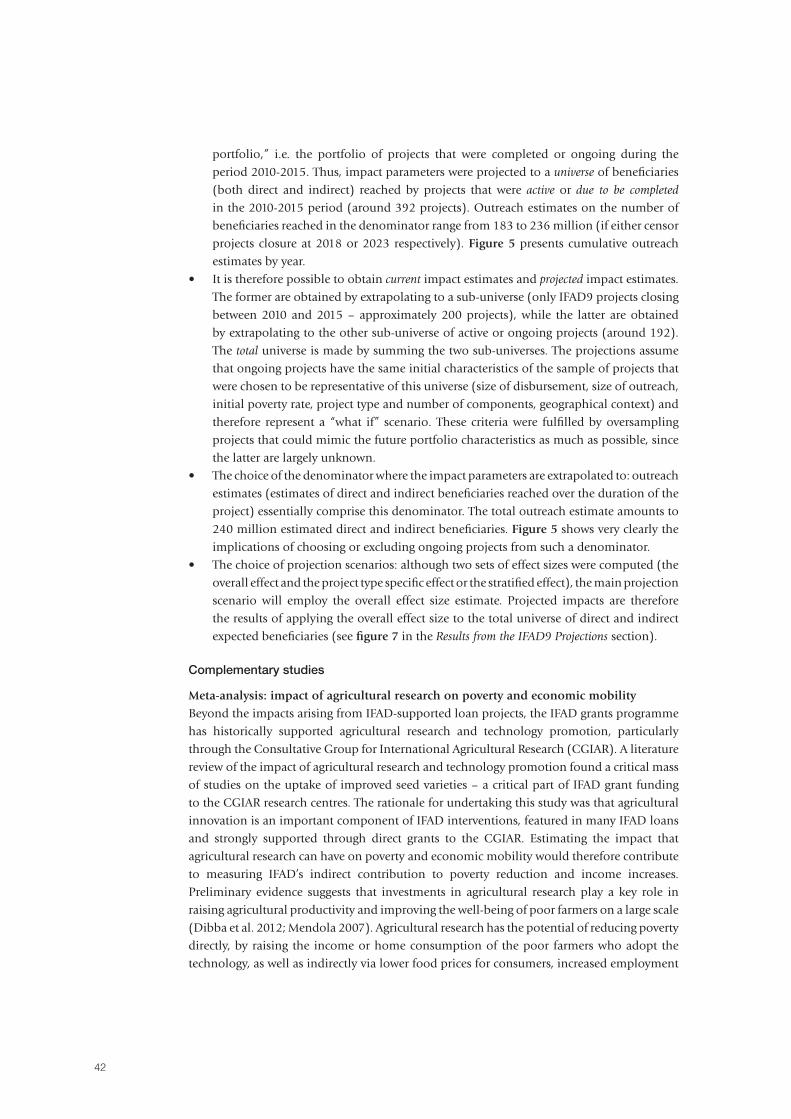
42
portfolio,” i.e. the portfolio of projects that were completed or ongoing during the
period 2010-2015. Thus, impact parameters were projected to a universe of beneficiaries
(both direct and indirect) reached by projects that were active or due to be completed
in the 2010-2015 period (around 392 projects). Outreach estimates on the number of
beneficiaries reached in the denominator range from 183 to 236 million (if either censor
projects closure at 2018 or 2023 respectively). Figure 5 presents cumulative outreach
estimates by year.
• It is therefore possible to obtain current impact estimates and projected impact estimates.
The former are obtained by extrapolating to a sub-universe (only IFAD9 projects closing
between 2010 and 2015 – approximately 200 projects), while the latter are obtained
by extrapolating to the other sub-universe of active or ongoing projects (around 192).
The total universe is made by summing the two sub-universes. The projections assume
that ongoing projects have the same initial characteristics of the sample of projects that
were chosen to be representative of this universe (size of disbursement, size of outreach,
initial poverty rate, project type and number of components, geographical context) and
therefore represent a “what if” scenario. These criteria were fulfilled by oversampling
projects that could mimic the future portfolio characteristics as much as possible, since
the latter are largely unknown.
• The choice of the denominator where the impact parameters are extrapolated to: outreach
estimates (estimates of direct and indirect beneficiaries reached over the duration of the
project) essentially comprise this denominator. The total outreach estimate amounts to
240 million estimated direct and indirect beneficiaries. Figure 5 shows very clearly the
implications of choosing or excluding ongoing projects from such a denominator.
• The choice of projection scenarios: although two sets of effect sizes were computed (the
overall effect and the project type specific effect or the stratified effect), the main projection
scenario will employ the overall effect size estimate. Projected impacts are therefore
the results of applying the overall effect size to the total universe of direct and indirect
expected beneficiaries (see figure 7 in the Results from the IFAD9 Projections section).
Complementary studies
Meta-analysis: impact of agricultural research on poverty and economic mobilityBeyond the impacts arising from IFAD-supported loan projects, the IFAD grants programme
has historically supported agricultural research and technology promotion, particularly
through the Consultative Group for International Agricultural Research (CGIAR). A literature
review of the impact of agricultural research and technology promotion found a critical mass
of studies on the uptake of improved seed varieties – a critical part of IFAD grant funding
to the CGIAR research centres. The rationale for undertaking this study was that agricultural
innovation is an important component of IFAD interventions, featured in many IFAD loans
and strongly supported through direct grants to the CGIAR. Estimating the impact that
agricultural research can have on poverty and economic mobility would therefore contribute
to measuring IFAD’s indirect contribution to poverty reduction and income increases.
Preliminary evidence suggests that investments in agricultural research play a key role in
raising agricultural productivity and improving the well-being of poor farmers on a large scale
(Dibba et al. 2012; Mendola 2007). Agricultural research has the potential of reducing poverty
directly, by raising the income or home consumption of the poor farmers who adopt the
technology, as well as indirectly via lower food prices for consumers, increased employment
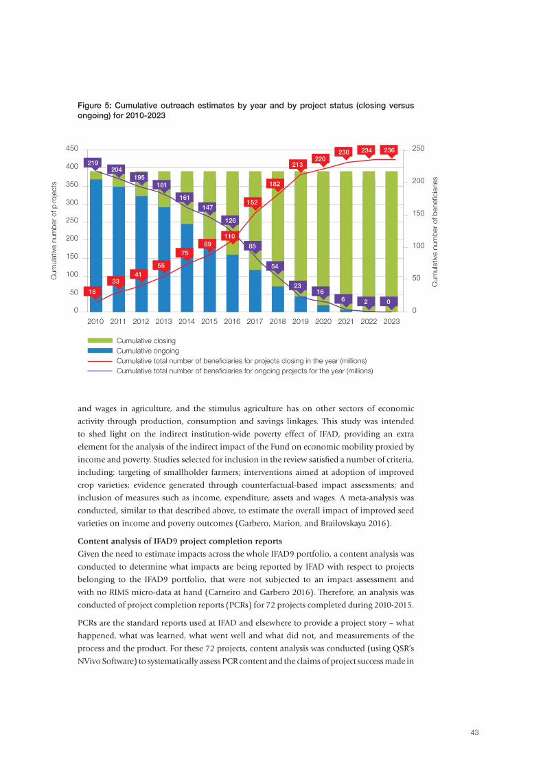
43
and wages in agriculture, and the stimulus agriculture has on other sectors of economic
activity through production, consumption and savings linkages. This study was intended
to shed light on the indirect institution-wide poverty effect of IFAD, providing an extra
element for the analysis of the indirect impact of the Fund on economic mobility proxied by
income and poverty. Studies selected for inclusion in the review satisfied a number of criteria,
including: targeting of smallholder farmers; interventions aimed at adoption of improved
crop varieties; evidence generated through counterfactual-based impact assessments; and
inclusion of measures such as income, expenditure, assets and wages. A meta-analysis was
conducted, similar to that described above, to estimate the overall impact of improved seed
varieties on income and poverty outcomes (Garbero, Marion, and Brailovskaya 2016).
Content analysis of IFAD9 project completion reports
Given the need to estimate impacts across the whole IFAD9 portfolio, a content analysis was
conducted to determine what impacts are being reported by IFAD with respect to projects
belonging to the IFAD9 portfolio, that were not subjected to an impact assessment and
with no RIMS micro-data at hand (Carneiro and Garbero 2016). Therefore, an analysis was
conducted of project completion reports (PCRs) for 72 projects completed during 2010-2015.
PCRs are the standard reports used at IFAD and elsewhere to provide a project story – what
happened, what was learned, what went well and what did not, and measurements of the
process and the product. For these 72 projects, content analysis was conducted (using QSR’s
NVivo Software) to systematically assess PCR content and the claims of project success made in
Figure 5: Cumulative outreach estimates by year and by project status (closing versus ongoing) for 2010-2023
450
400
350
300
250
200
150
100
50
0
250
200
150
100
50
0
Cumulative closingCumulative ongoingCumulative total number of beneficiaries for projects closing in the year (millions)Cumulative total number of beneficiaries for ongoing projects for the year (millions)
Cum
ulat
ive
num
ber
of p
roje
cts
Cum
ulat
ive
num
ber
of b
enef
icia
ries
2010 2011 2012 2013 2014 2015 2016 2017 2018 2019 2020 2021 2022 2023
219
18
204
33
195
41
181
55
161
75
147
89
126
110
85
152
54
182
23
213
16
220
6
230
2
234
0
236

44
those documents. Content analysis is a research technique for systematically interpreting and
coding textual material (such as PCRs) and can be defined as “any methodical measurement
applied to text (or other symbolic material) for social scientific purposes” (Shapiro and
Markoff 1997). The literature has stressed various aspects of content analysis, from its capacity
to generate quantitative descriptions by analysing word counts (Berelson 1952; Silverman
2011) to its ability to help researchers draw inferences from a text by breaking that text down
into discrete units of manageable data that can then be meaningfully reorganized (Weber
1990). Others have argued that content analysis is an approach echoing “grounded” theory
and other strongly inductive approaches to data analysis (Strauss 1987).
The methodology of content analysis was paired with an IFAD-specific conceptual framework
for analysing project documentation (the PCRs). This thematic indicators framework was
designed to assess the current state of evidence in IFAD project documentation in order
to find evidentiary support for outputs, outcomes and impacts across the different project
types. The framework was flexibly designed to capture various types of results across the
following nine different themes: agricultural production, human capital, commerce and
value chains, women’s empowerment, food security and health, capacity to innovate, policies
and institutions, environmental sustainability, and economic mobility. For the IFAD9 IAI,
content analysis has been used to determine: what benefits are perceived; what evidence
exists in project documentation of IFAD’s contribution; and what sources of evidence are
used to support claims concerning IFAD project results.
Randomized controlled trials (3-6 studies)Lastly, the IFAD9 IAI also includes six ex ante impact assessments conducted using RCTs, or
quasi-experimental designs. These studies are prospective studies (therefore, ex ante) – for
example, studies that are designed prior to the implementation of new projects. They can be
regarded as innovative evaluation designs that should be incorporated at project inception.
Recall that the RCT methodology entails an impact assessment design in which random
assignment16 is used to allocate the intervention among members of the eligible population.
Randomization ensures that the group that receives an intervention (the treatment group)
and the group that does not (the control group) have comparable characteristics; therefore,
through this methodology one could conclude that the difference in the outcome observed
(for instance, poverty reduction) is the causal effect of the intervention.
Given the time involved and the experimental nature in the field of agricultural and rural
development, it became apparent that these studies could only provide estimates of the impact
of IFAD-supported projects once completed, reaching beyond the IFAD9 period. Hence only
baseline results are expected during the IFAD9 period, and not the full evaluations results.
The latter will be available by 2018-2020, depending on the specific duration of each project.
This set of studies have been funded by a grant programme launched by the International
Initiative for Impact Evaluation (3ie), named the Agricultural Innovation Thematic Window.
This grant scheme is supported by the Bill & Melinda Gates Foundation and DFID. It has
funded 15 ex ante impact assessments of interventions associated with IFAD and the Alliance
for a Green Revolution in Africa (AGRA), aiming to increase the stock of rigorous evidence
on what works in agricultural innovation in South Asia and sub-Saharan Africa in the areas of
knowledge transfer, contractual arrangements, technology adoption and soil health.
16. An intervention design in which members of the eligible population are assigned at random to either the treatment group or the control group (i.e. random assignment). Thus, whether someone is in the treatment or control group is solely a matter of chance and not a function of any of their characteristics (either observed or unobserved).
45
IFAD engaged with 3ie and the relevant stakeholders in order to select projects that were at design phase and that were deemed most suitable for an experimental design (an RCT). Initially, 30 new projects were selected, based on the following ad hoc purposive criteria:• Timing – new IFAD-supported projects in the design phase, submitted to the December
2013 and April 2014 Executive Board meetings• Geographical coverage – Africa and South Asia• Thematic relevance.
In order to determine thematic relevance, a stakeholders’ consultation workshop was held in Nairobi in June 2013 to decide on key research questions where learning should be sought. To this end, joint research areas for both IFAD and AGRA in the field of agricultural innovation were identified in a participatory manner. Four key research questions, revolving around the topic of adoption of new technologies, were identified. The specific research questions are provided in the section on the Experimental designs (RCTs) under the 3ie Agricultural Innovation
Window in the Appendices.
To date, five RCTs (table 7 in the section on the Experimental designs (RCTs) under the 3ie
Agricultural Innovation Window in the Appendices17) were incorporated at project inception and their design is currently ongoing. Additional resources have been identified by 3ie for one more study, bringing the total to six RCTs which have been initiated during the IFAD9 period (2013-2015) and will be completed over IFAD10 (2015-2018) and beyond.
These studies will also help derive lessons on methodology, the potential of using these approaches and the challenges of implementing ex ante impact assessments.
17. Including: (1) Promoting Agricultural Commercialization and Enterprises (PACE) in Bangladesh, in partnership with Palli Karma-Sahayak Foundation (PKSF); (2) Agriculture Services Programme for Innovation, Resilience and Extension (ASPIRE) in Cambodia, in partnership with IFPRI; (3) Ghana Agricultural Sector Investment Programme (GASIP) in Ghana, in partnership with IFPRI and IPA; (4) Smallholder Market-Led Project (SMLP) in Swaziland, in partnership with IPA; (5) Vegetable Oil Development Project (VODP 2) in Uganda, in partnership with Centro Studi Luca d’Agliano (LdA); and (6) Rural Finance Expansion Programme (RUFEP) in Zambia, in partnership with Mannheim University.
46
Overall, the approach to the IFAD9 IAI was systematic and comprehensive. Of course, much
of the assessment of impact is backward-looking, as data were collected ex post, which
presents significant challenges. Moreover, prior to this initiative, IFAD had limited experience
with analysis designed to attribute impact to IFAD-funded projects. As such, the process was
intentionally designed for lesson-learning.
Lessons on methods
Prior to providing estimates of impact and portfolio projections of those receiving benefits,
the methodological lessons of the process must be noted. This is critical not only for
improving impact estimates for the next replenishment period IFAD10 (2016-2018) and
beyond, but also in putting results in the context of methodological challenges. Lessons are
learned through: reflection on the process of setting up the methodological approach; efforts
to administer ex post and ex ante impact assessments in the field; analysis of data coming out
of the exercise; and discussions with IFAD staff and others on the exercise’s merits.
First, random project selection to represent the portfolio is difficult to implement and limits
learning. Projects were selected to be representative of IFAD’s portfolio and to respond to
the need to measure aggregate impact. This process is potentially advantageous for arriving
at aggregate figures, but is difficult to implement. Even in this exercise, 9 of the 24 Deep
Dives were purposefully selected, as not all projects were suitable for assessment. This is an
even greater issue with ex ante impact assessments, as it is hard to predict a future portfolio.
Moreover, random selection limits learning, as this selection procedure responds to an
accountability mandate and does not focus on where learning might be the greatest.
Second, focusing on a poverty line, or any individual indicator, inadequately assesses IFAD’s
investments and fails to carefully analyse a project’s theory of change – that is, the causal
chain or pathway through which impact occurs. The focus, then, is potentially on indicators
that may not be the most relevant to a given project or to IFAD’s portfolio as a whole. Greater
consideration is needed of IFAD’s portfolio of interventions, the theory of change of those
interventions and the corresponding set of anticipated aggregate impacts.
Third, designing impact assessments ex post is challenging and reduces the value of
impact assessments. As IFAD9 IAI assessed impact through ex post approaches, analysis
required collecting data on projects that were no longer operational in a context in which
documentation was scarce. In many cases, the existing project information was very limited
and project teams were no longer available. Identifying beneficiaries within a targeted region
was challenging, as was accessing adequate project data. Creating a reasonable counterfactual
after project completion is demanding at best, and at worst impossible. There is generally a
Results: lessons, estimates and projections
47
tendency to underestimate impact if projects are poverty-targeted, as control groups may be
better off than the treatment groups. This creates a situation in which a successful pro-poor
targeting strategy can lead to the appearance of limited benefit. The ex post approach to
impact assessment leads to significant difficulties in adequately estimating impact. Impact
assessments should be therefore designed ex ante; the ideal would be to evolve towards a
system where development effectiveness is addressed at entry and not at exit (i.e. a system
that allows one to design sound development projects, monitor their progress, and measure
their results and impact across the project life cycle).
Fourth, impact assessments are most effective when they are built on strong logframes and
M&E systems, and generally developed at the project design and readiness stage. When done
properly, logframes articulate a clear theory of change for the project, highlight the impact
pathway and note the means by which the latter is to be measured. When well designed and
executed, an M&E system allows for clear identification of beneficiaries and provides a sense
of what outputs have been provided to beneficiaries in a project. The timing of baseline
and follow-up data collection also affects the ability to adequately assess impact and the
questions that can be answered. Thus, it is crucial that impact assessments be designed ex
ante and in conjunction with project design.
Lastly, buy-in by IFAD staff and national governments is critical in implementing impact
assessments and enhancing the learning generated. Those who specialize in impact
assessment are often not specialists in certain thematic areas or countries, and do not have
the necessary experience to understand the details of project implementation. They also do
not always know what compelling policy questions must be addressed. On the other hand,
IFAD and government staff often do not understand the technical basis of impact assessment
and the requirements for achieving attribution. As a result, the quality of impact assessments
is limited by a lack of buy-in and communication among key actors.
Estimates and projections of impacts
Given the focus on aggregate rather than project-level analysis, results are projected to the
portfolio of projects closed and ongoing during 2010-2015, the total universe described in
step 7 of the section on the Results from the IFAD9 projections.
In order for a project to have an impact, it is critical to ensure that its key outputs are
delivered; a consideration of these outputs is therefore the logical point of departure. From
an analysis of IFAD’s projects portfolio, numerous critical outputs emerge (table 2). For all
closed and ongoing projects during the 2010-2015 period, 139 million people and 24 million
households received project interventions. A range of activities targeted poor rural people,
designed to broadly improve their well-being. These beneficiaries included 18.0 million
active borrowers and 26.6 million voluntary savers, highlighting IFAD’s focus on financial
inclusion. Numerous farmers have been trained in agricultural practices, including 4.4 million
in crop production technologies, 1.6 million in livestock production and 1.4 million in
natural resource management. Improvements in agricultural activities have been promoted,
leading to 5.0 million hectares under improved management practices. This has largely been
accomplished through strengthening farmers’ organizations and thousands of community
groups, including market, productive, infrastructure, agricultural and livestock groups. Many
of these have been created with women in leadership positions. The data suggest that IFAD’s
investment in rural people is leading to significant outputs.
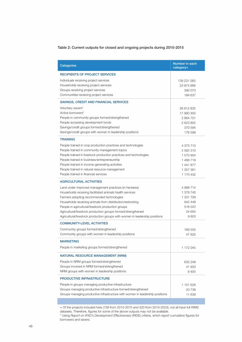
48
Table 2: Current outputs for closed and ongoing projects during 2010-2015
CategoriesNumber in each category+
RECIPIENTS OF PROJECT SERVICES
Individuals receiving project services
Households receiving project services
Groups receiving project services
Communities receiving project services
139 231 083
23 874 666
390 073
184 637
SAVINGS, CREDIT AND FINANCIAL SERVICES
Voluntary savers*
Active borrowers*
People in community groups formed/strengthened
People accessing development funds
Savings/credit groups formed/strengthened
Savings/credit groups with women in leadership positions
26 612 835
17 990 300
2 864 701
2 623 855
370 594
176 599
TRAINING
People trained in crop production practices and technologies
People trained in community management topics
People trained in livestock production practices and technologies
People trained in business/entrepreneurship
People trained in income-generating activities
People trained in natural resource management
People trained in financial services
4 375 710
2 582 310
1 570 904
1 466 719
1 441 877
1 357 361
1 170 432
AGRICULTURAL ACTIVITIES
Land under improved management practices (in hectares)
Households receiving facilitated animals health services
Farmers adopting recommended technologies
Households receiving animals from distribution/restocking
People in agricultural/livestock production groups
Agricultural/livestock production groups formed/strengthened
Agricultural/livestock production groups with women in leadership positions
4 998 714
1 379 740
1 331 709
942 448
516 022
24 655
9 603
COMMUNITY-LEVEL ACTIVITIES
Community groups formed/strengthened
Community groups with women in leadership positions169 555
47 625
MARKETING
People in marketing groups formed/strengthened 1 172 045
NATURAL RESOURCE MANAGEMENT (NRM)
People in NRM groups formed/strengthened
Groups involved in NRM formed/strengthened
NRM groups with women in leadership positions
632 248
41 933
9 405
PRODUCTIVE INFRASTRUCTURE
People in groups managing productive infrastructure
Groups managing productive infrastructure formed/strengthened
Groups managing productive infrastructure with women in leadership positions
1 151 628
23 736
11 639
+ Of the projects included here (158 from 2010-2015 and 320 from 2010-2023), not all have full RIMS datasets. Therefore, figures for some of the above outputs may not be available.* Using Report on IFAD’s Development Effectiveness (RIDE) criteria, which report cumulative figures for borrowers and savers.
49
Results on IFAD9 aggregate impacts: meta-analysis
This section reports on the results of the synthesis or aggregation of the 37 quantitative IFAD9
ex post Impact Assessments (22 Deep Dives, 14 Shallow Dives and 1 multiple-project impact
assessment, see table 3). Outcome indicators across studies were grouped into six impact
domains, namely economic mobility, poverty outcomes, resilience, nutrition, agriculture,
livestock and gender empowerment. Within these broad impact domains, the following
outcome indicators were analysed, specifically:
• Asset indices (asset indices based on durables only, on productive farm assets only, on all
assets [overall])
• Expenditure outcomes (food, non-food and total, both at household-level and per capita)
• Income
• Poverty outcomes based on the above-mentioned asset indices
• Resilience proxies (ability to recover, severity of shocks, exposure to shocks and frequency
of shocks)
• Dietary diversity (including food consumed and number of meals)
• Agricultural diversity (crop choice, number of crops grown)
• Agricultural revenue
• Yields (various crops)
• Livestock indices (total, small livestock, large livestock and poultry count indices)
• Gender empowerment dimensions (participation to activities, access and control
over resources).
It is important to note that not all studies reported on all outcomes, as the latter were conditional
on the project-specific causal chain and data availability (see table 4).
As mentioned in the section on Data and methods: concepts and approach, designing impact
assessments of agricultural projects can be challenging due to the wide range of factors that can
influence agricultural outcomes, as well as due to biases caused by self-selection of individuals
and communities into projects. Thus, the differences in outcomes between beneficiaries and
non-beneficiaries can be due to differential pre-existing conditions rather than attributable to
the project under evaluation.
In view of the above, the IFAD9 IAI studies were also appraised in terms of internal and statistical
conclusion validity (figures 6 and 7); this involved an assessment of risk of bias, conducted on
an individual study basis. Nearly 52 per cent of the studies were classified as low and medium
risk of bias and were therefore retained in the meta-analysis.
High risk of bias studies were largely the ones selected in a purposeful manner (see figure 6)
and shared the following characteristics (see figure 7): comparison groups tended to be sampled
in the same areas where the treatment was administered; there were less than 10 matching
covariates (indicating that the statistical quality of propensity score matching could be poorer);
and surveys were conducted well after project closure, implying that such studies could be
exposed to more confounding factors that increase the level of bias.
The results of the meta-analysis are reported by outcome rather than by study. Table 4 shows
the distribution of outcomes by study design, by impact domain and by region. Note that the
number of outcomes reflects the larger occurrence of studies in certain regions (for instance,
APR) which is proportional to the size of the regional portfolio. Besides poverty outcomes,
which were a compulsory requirement of the studies, other outcomes (specifically, nutritional,
resilience and gender-specific outcomes) were chosen when found relevant to the project-
specific theory of change and contingent on data availability.
Table 2: Current outputs for closed and ongoing projects during 2010-2015
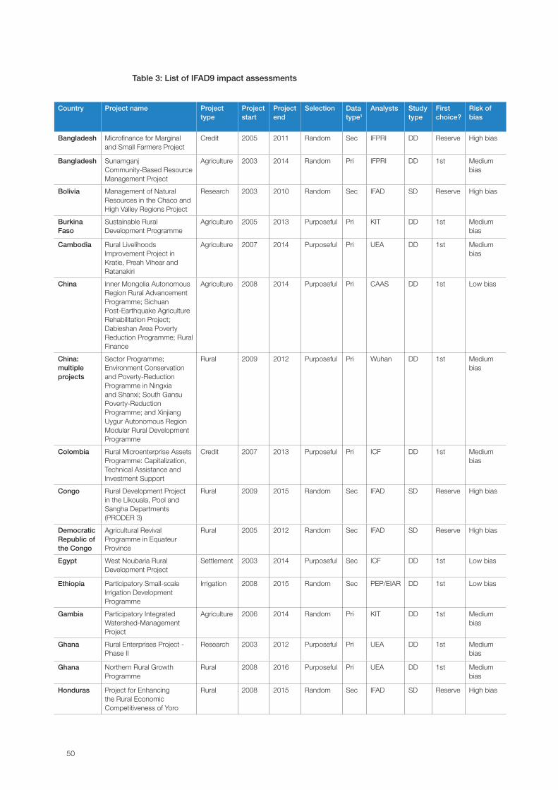
50
Country Project name Project type
Project start
Project end
Selection Data type1
Analysts Study type
First choice?
Risk of bias
Bangladesh Microfinance for Marginal and Small Farmers Project
Credit 2005 2011 Random Sec IFPRI DD Reserve High bias
Bangladesh Sunamganj Community-Based Resource Management Project
Agriculture 2003 2014 Random Pri IFPRI DD 1st Medium bias
Bolivia Management of Natural Resources in the Chaco and High Valley Regions Project
Research 2003 2010 Random Sec IFAD SD Reserve High bias
Burkina Faso
Sustainable Rural Development Programme
Agriculture 2005 2013 Purposeful Pri KIT DD 1st Medium bias
Cambodia Rural Livelihoods Improvement Project in Kratie, Preah Vihear and Ratanakiri
Agriculture 2007 2014 Purposeful Pri UEA DD 1st Medium bias
China Inner Mongolia Autonomous Region Rural Advancement Programme; Sichuan Post-Earthquake Agriculture Rehabilitation Project; Dabieshan Area Poverty Reduction Programme; Rural Finance
Agriculture 2008 2014 Purposeful Pri CAAS DD 1st Low bias
China: multiple projects
Sector Programme; Environment Conservation and Poverty-Reduction Programme in Ningxia and Shanxi; South Gansu Poverty-Reduction Programme; and Xinjiang Uygur Autonomous Region Modular Rural Development Programme
Rural 2009 2012 Purposeful Pri Wuhan DD 1st Medium bias
Colombia Rural Microenterprise Assets Programme: Capitalization, Technical Assistance and Investment Support
Credit 2007 2013 Purposeful Pri ICF DD 1st Medium bias
Congo Rural Development Project in the Likouala, Pool and Sangha Departments (PRODER 3)
Rural 2009 2015 Random Sec IFAD SD Reserve High bias
DemocraticRepublic ofthe Congo
Agricultural Revival Programme in Equateur Province
Rural 2005 2012 Random Sec IFAD SD Reserve High bias
Egypt West Noubaria Rural Development Project
Settlement 2003 2014 Purposeful Sec ICF DD 1st Low bias
Ethiopia Participatory Small-scale Irrigation Development Programme
Irrigation 2008 2015 Random Sec PEP/EIAR DD 1st Low bias
Gambia Participatory Integrated Watershed-Management Project
Agriculture 2006 2014 Random Pri KIT DD 1st Medium bias
Ghana Rural Enterprises Project - Phase II
Research 2003 2012 Purposeful Pri UEA DD 1st Medium bias
Ghana Northern Rural Growth Programme
Rural 2008 2016 Purposeful Pri UEA DD 1st Medium bias
Honduras Project for Enhancing the Rural Economic Competitiveness of Yoro
Rural 2008 2015 Random Sec IFAD SD Reserve High bias
Table 3: List of IFAD9 impact assessments
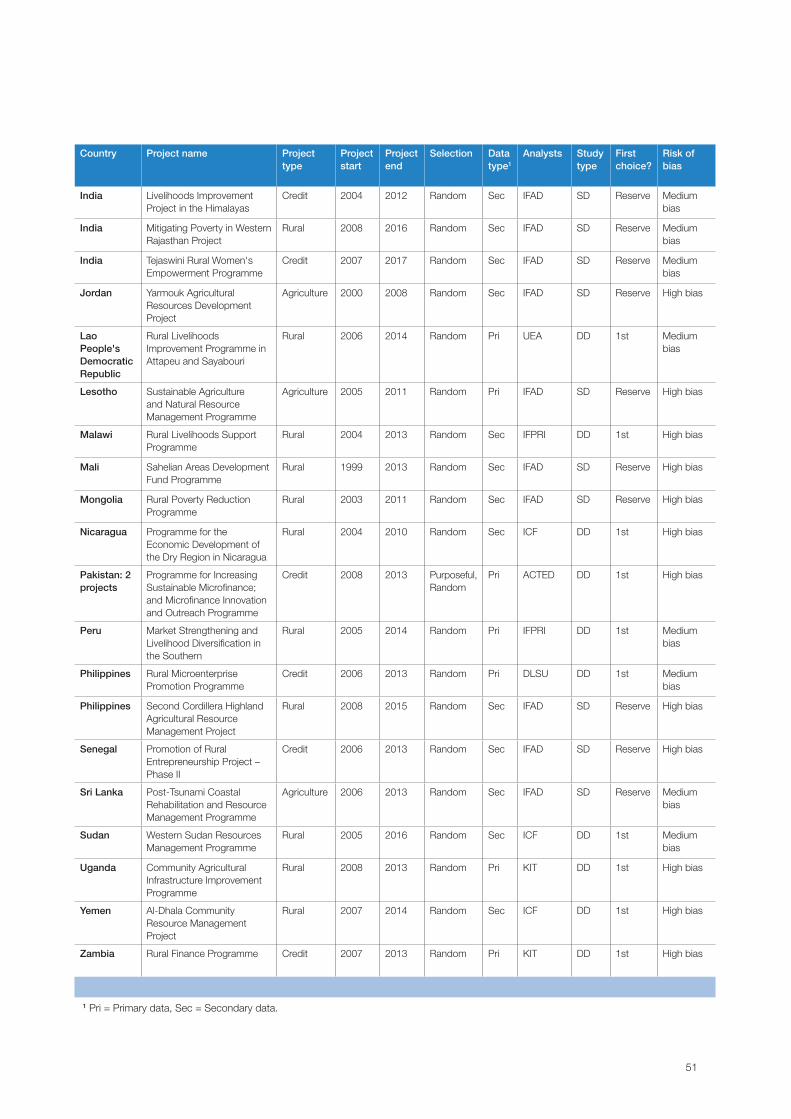
51
Country Project name Project type
Project start
Project end
Selection Data type1
Analysts Study type
First choice?
Risk of bias
India Livelihoods Improvement Project in the Himalayas
Credit 2004 2012 Random Sec IFAD SD Reserve Medium bias
India Mitigating Poverty in Western Rajasthan Project
Rural 2008 2016 Random Sec IFAD SD Reserve Medium bias
India Tejaswini Rural Women's Empowerment Programme
Credit 2007 2017 Random Sec IFAD SD Reserve Medium bias
Jordan Yarmouk Agricultural Resources Development Project
Agriculture 2000 2008 Random Sec IFAD SD Reserve High bias
Lao People's Democratic Republic
Rural Livelihoods Improvement Programme in Attapeu and Sayabouri
Rural 2006 2014 Random Pri UEA DD 1st Medium bias
Lesotho Sustainable Agriculture and Natural Resource Management Programme
Agriculture 2005 2011 Random Pri IFAD SD Reserve High bias
Malawi Rural Livelihoods Support Programme
Rural 2004 2013 Random Sec IFPRI DD 1st High bias
Mali Sahelian Areas Development Fund Programme
Rural 1999 2013 Random Sec IFAD SD Reserve High bias
Mongolia Rural Poverty Reduction Programme
Rural 2003 2011 Random Sec IFAD SD Reserve High bias
Nicaragua Programme for the Economic Development of the Dry Region in Nicaragua
Rural 2004 2010 Random Sec ICF DD 1st High bias
Pakistan: 2 projects
Programme for Increasing Sustainable Microfinance; and Microfinance Innovation and Outreach Programme
Credit 2008 2013 Purposeful,Random
Pri ACTED DD 1st High bias
Peru Market Strengthening and Livelihood Diversification in the Southern
Rural 2005 2014 Random Pri IFPRI DD 1st Medium bias
Philippines Rural Microenterprise Promotion Programme
Credit 2006 2013 Random Pri DLSU DD 1st Medium bias
Philippines Second Cordillera Highland Agricultural Resource Management Project
Rural 2008 2015 Random Sec IFAD SD Reserve High bias
Senegal Promotion of Rural Entrepreneurship Project – Phase II
Credit 2006 2013 Random Sec IFAD SD Reserve High bias
Sri Lanka Post-Tsunami Coastal Rehabilitation and Resource Management Programme
Agriculture 2006 2013 Random Sec IFAD SD Reserve Medium bias
Sudan Western Sudan Resources Management Programme
Rural 2005 2016 Random Sec ICF DD 1st Medium bias
Uganda Community Agricultural Infrastructure Improvement Programme
Rural 2008 2013 Random Pri KIT DD 1st High bias
Yemen Al-Dhala Community Resource Management Project
Rural 2007 2014 Random Sec ICF DD 1st High bias
Zambia Rural Finance Programme Credit 2007 2013 Random Pri KIT DD 1st High bias
1 Pri = Primary data, Sec = Secondary data.
Table 3: List of IFAD9 impact assessments
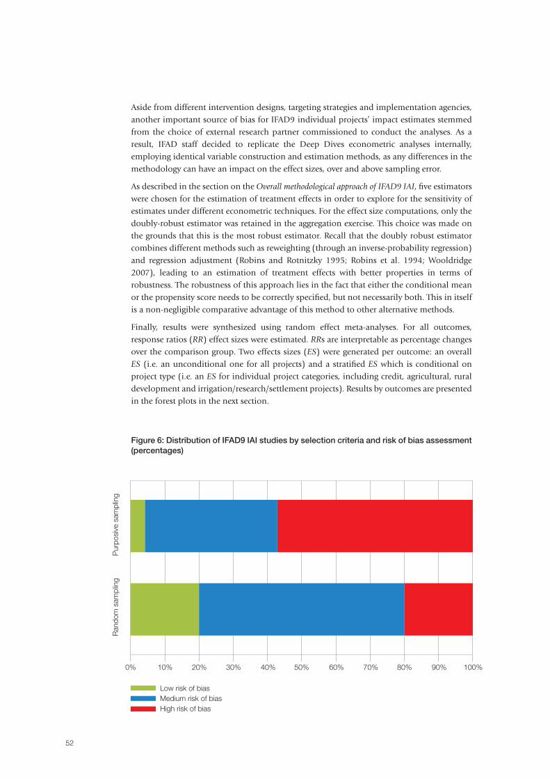
52
Aside from different intervention designs, targeting strategies and implementation agencies, another important source of bias for IFAD9 individual projects’ impact estimates stemmed from the choice of external research partner commissioned to conduct the analyses. As a result, IFAD staff decided to replicate the Deep Dives econometric analyses internally, employing identical variable construction and estimation methods, as any differences in the methodology can have an impact on the effect sizes, over and above sampling error.
As described in the section on the Overall methodological approach of IFAD9 IAI, five estimators were chosen for the estimation of treatment effects in order to explore for the sensitivity of estimates under different econometric techniques. For the effect size computations, only the doubly-robust estimator was retained in the aggregation exercise. This choice was made on the grounds that this is the most robust estimator. Recall that the doubly robust estimator combines different methods such as reweighting (through an inverse-probability regression) and regression adjustment (Robins and Rotnitzky 1995; Robins et al. 1994; Wooldridge 2007), leading to an estimation of treatment effects with better properties in terms of robustness. The robustness of this approach lies in the fact that either the conditional mean or the propensity score needs to be correctly specified, but not necessarily both. This in itself is a non-negligible comparative advantage of this method to other alternative methods.
Finally, results were synthesized using random effect meta-analyses. For all outcomes, response ratios (RR) effect sizes were estimated. RRs are interpretable as percentage changes over the comparison group. Two effects sizes (ES) were generated per outcome: an overall ES (i.e. an unconditional one for all projects) and a stratified ES which is conditional on project type (i.e. an ES for individual project categories, including credit, agricultural, rural development and irrigation/research/settlement projects). Results by outcomes are presented in the forest plots in the next section.
Figure 6: Distribution of IFAD9 IAI studies by selection criteria and risk of bias assessment (percentages)
0% 10% 20% 30% 40% 50% 60% 70% 80% 90% 100%
Pur
posi
ve s
ampl
ing
Ran
dom
sam
plin
g
Low risk of biasMedium risk of biasHigh risk of bias
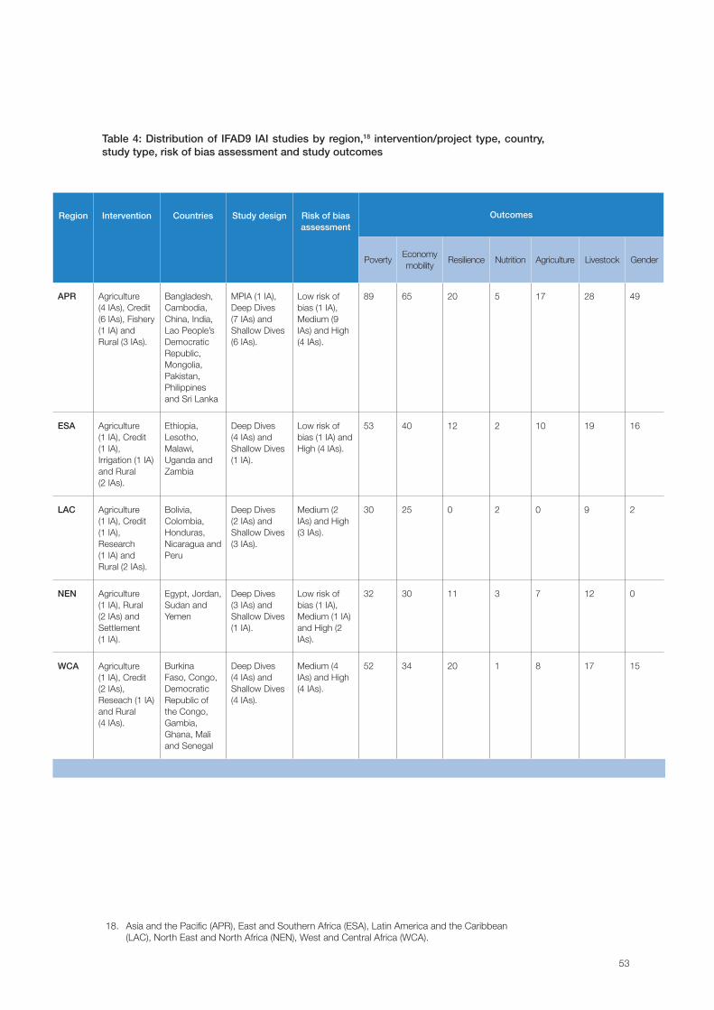
53
Table 4: Distribution of IFAD9 IAI studies by region,18 intervention/project type, country, study type, risk of bias assessment and study outcomes
Region Intervention Countries Study design Risk of bias assessment
Outcomes
PovertyEconomy mobility
Resilience Nutrition Agriculture Livestock Gender
APR Agriculture (4 IAs), Credit (6 IAs), Fishery (1 IA) and Rural (3 IAs).
Bangladesh, Cambodia, China, India, Lao People’s Democratic Republic, Mongolia, Pakistan, Philippines and Sri Lanka
MPIA (1 IA), Deep Dives (7 IAs) and Shallow Dives (6 IAs).
Low risk of bias (1 IA), Medium (9 IAs) and High (4 IAs).
89 65 20 5 17 28 49
ESA Agriculture (1 IA), Credit (1 IA), Irrigation (1 IA) and Rural (2 IAs).
Ethiopia, Lesotho, Malawi, Uganda and Zambia
Deep Dives (4 IAs) and Shallow Dives (1 IA).
Low risk of bias (1 IA) and High (4 IAs).
53 40 12 2 10 19 16
LAC Agriculture (1 IA), Credit (1 IA), Research (1 IA) and Rural (2 IAs).
Bolivia, Colombia, Honduras, Nicaragua and Peru
Deep Dives (2 IAs) and Shallow Dives (3 IAs).
Medium (2 IAs) and High (3 IAs).
30 25 0 2 0 9 2
NEN Agriculture (1 IA), Rural (2 IAs) and Settlement (1 IA).
Egypt, Jordan, Sudan and Yemen
Deep Dives (3 IAs) and Shallow Dives (1 IA).
Low risk of bias (1 IA), Medium (1 IA) and High (2 IAs).
32 30 11 3 7 12 0
WCA Agriculture (1 IA), Credit (2 IAs), Reseach (1 IA) and Rural (4 IAs).
Burkina Faso, Congo, Democratic Republic of the Congo, Gambia, Ghana, Mali and Senegal
Deep Dives (4 IAs) and Shallow Dives (4 IAs).
Medium (4 IAs) and High (4 IAs).
52 34 20 1 8 17 15
18. Asia and the Pacific (APR), East and Southern Africa (ESA), Latin America and the Caribbean (LAC), North East and North Africa (NEN), West and Central Africa (WCA).
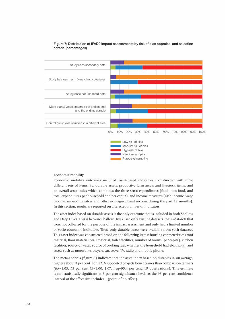
54
Economic mobility
Economic mobility outcomes included: asset-based indicators (constructed with three
different sets of items, i.e. durable assets, productive farm assets and livestock items, and
an overall asset index which combines the three sets); expenditures (food, non-food, and
total expenditures per household and per capita); and income measures (cash income, wage
income, in-kind transfers and other non-agricultural income during the past 12 months).
In this section, results are reported on a selected number of indicators.
The asset index based on durable assets is the only outcome that is included in both Shallow
and Deep Dives. This is because Shallow Dives used only existing datasets, that is datasets that
were not collected for the purpose of the impact assessment and only had a limited number
of socio-economic indicators. Thus, only durable assets were available from such datasets.
This asset index was constructed based on the following items: housing characteristics (roof
material, floor material, wall material, toilet facilities, number of rooms (per capita), kitchen
facilities, source of water, source of cooking fuel, whether the household had electricity), and
assets such as motorbike, bicycle, car, stove, TV, radio and mobile phone.
The meta-analysis (figure 8) indicates that the asset index based on durables is, on average,
higher (about 3 per cent) for IFAD-supported projects beneficiaries than comparison farmers
(RR=1.03, 95 per cent CI=1.00, 1.07, I-sq=95.4 per cent; 19 observations). This estimate
is not statistically significant at 5 per cent significance level, as the 95 per cent confidence
interval of the effect size includes 1 (point of no effect).
Figure 7: Distribution of IFAD9 impact assessments by risk of bias appraisal and selection criteria (percentages)
Low risk of biasMedium risk of biasHigh risk of biasRandom samplingPurposive sampling
Study uses secondary data
Study has less than 10 matching covariates
Control group was sampled in a different area
Study does not use recall data
More than 2 years separate the project endand the endline sample
234 236
0% 10% 20% 30% 40% 50% 60% 70% 80% 90% 100%
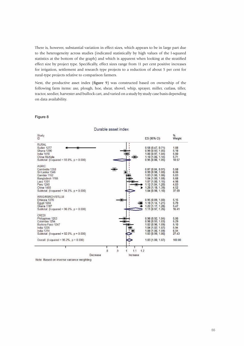
55
There is, however, substantial variation in effect sizes, which appears to be in large part due to the heterogeneity across studies (indicated statistically by high values of the I-squared statistics at the bottom of the graph) and which is apparent when looking at the stratified effect size by project type. Specifically, effect sizes range from 11 per cent positive increases for irrigation, settlement and research type projects to a reduction of about 5 per cent for rural-type projects relative to comparison farmers.
Next, the productive asset index (figure 9) was constructed based on ownership of the following farm items: axe, plough, hoe, shear, shovel, whip, sprayer, miller, cutlass, tiller, tractor, seedier, harvester and bullock cart, and varied on a study by study case basis depending on data availability.
Figure 8
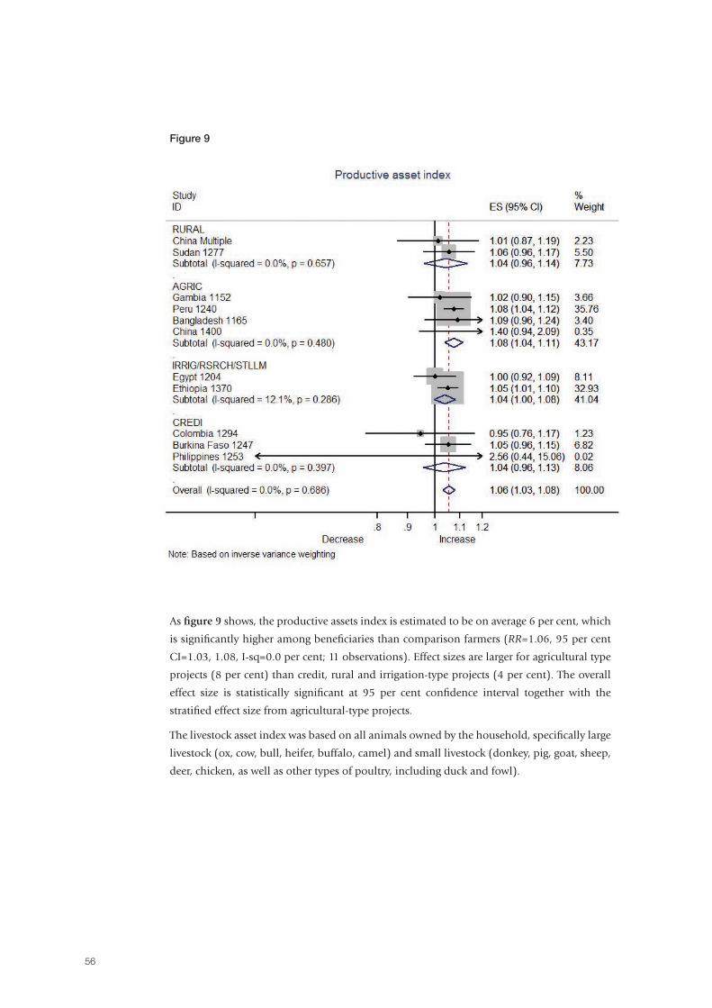
56
As figure 9 shows, the productive assets index is estimated to be on average 6 per cent, which
is significantly higher among beneficiaries than comparison farmers (RR=1.06, 95 per cent
CI=1.03, 1.08, I-sq=0.0 per cent; 11 observations). Effect sizes are larger for agricultural type
projects (8 per cent) than credit, rural and irrigation-type projects (4 per cent). The overall
effect size is statistically significant at 95 per cent confidence interval together with the
stratified effect size from agricultural-type projects.
The livestock asset index was based on all animals owned by the household, specifically large
livestock (ox, cow, bull, heifer, buffalo, camel) and small livestock (donkey, pig, goat, sheep,
deer, chicken, as well as other types of poultry, including duck and fowl).
Figure 9
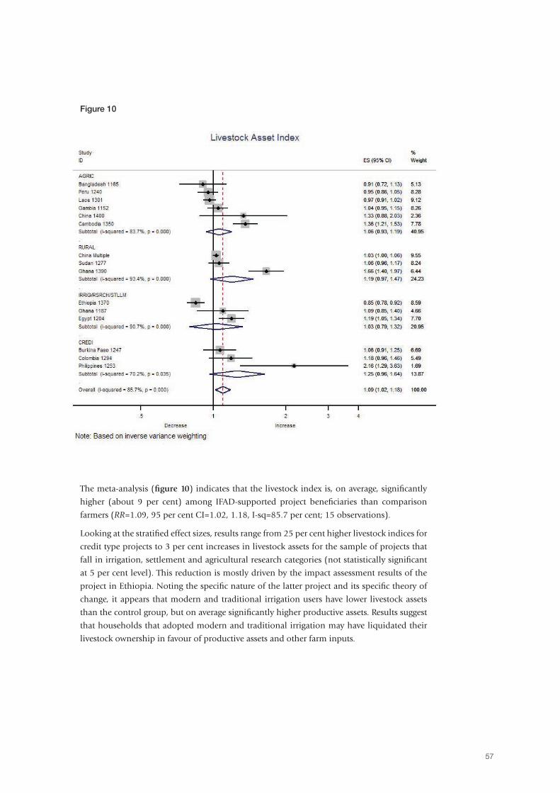
57
The meta-analysis (figure 10) indicates that the livestock index is, on average, significantly
higher (about 9 per cent) among IFAD-supported project beneficiaries than comparison
farmers (RR=1.09, 95 per cent CI=1.02, 1.18, I-sq=85.7 per cent; 15 observations).
Looking at the stratified effect sizes, results range from 25 per cent higher livestock indices for
credit type projects to 3 per cent increases in livestock assets for the sample of projects that
fall in irrigation, settlement and agricultural research categories (not statistically significant
at 5 per cent level). This reduction is mostly driven by the impact assessment results of the
project in Ethiopia. Noting the specific nature of the latter project and its specific theory of
change, it appears that modern and traditional irrigation users have lower livestock assets
than the control group, but on average significantly higher productive assets. Results suggest
that households that adopted modern and traditional irrigation may have liquidated their
livestock ownership in favour of productive assets and other farm inputs.
Figure 10
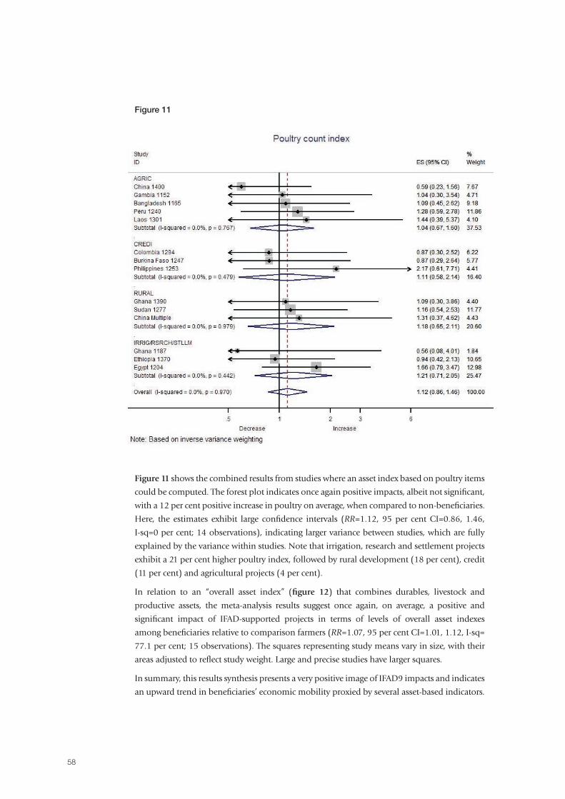
58
Figure 11 shows the combined results from studies where an asset index based on poultry items
could be computed. The forest plot indicates once again positive impacts, albeit not significant,
with a 12 per cent positive increase in poultry on average, when compared to non-beneficiaries.
Here, the estimates exhibit large confidence intervals (RR=1.12, 95 per cent CI=0.86, 1.46,
I-sq=0 per cent; 14 observations), indicating larger variance between studies, which are fully
explained by the variance within studies. Note that irrigation, research and settlement projects
exhibit a 21 per cent higher poultry index, followed by rural development (18 per cent), credit
(11 per cent) and agricultural projects (4 per cent).
In relation to an “overall asset index” (figure 12) that combines durables, livestock and
productive assets, the meta-analysis results suggest once again, on average, a positive and
significant impact of IFAD-supported projects in terms of levels of overall asset indexes
among beneficiaries relative to comparison farmers (RR=1.07, 95 per cent CI=1.01, 1.12, I-sq=
77.1 per cent; 15 observations). The squares representing study means vary in size, with their
areas adjusted to reflect study weight. Large and precise studies have larger squares.
In summary, this results synthesis presents a very positive image of IFAD9 impacts and indicates
an upward trend in beneficiaries’ economic mobility proxied by several asset-based indicators.
Figure 11
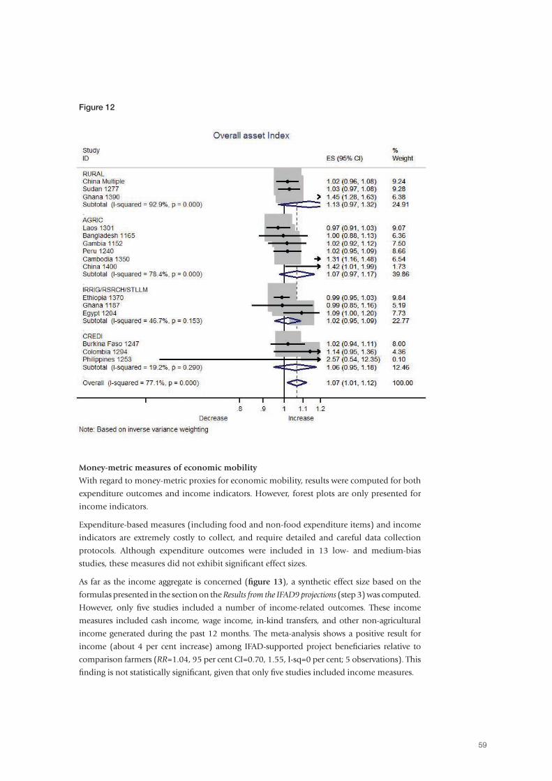
59
Money-metric measures of economic mobility
With regard to money-metric proxies for economic mobility, results were computed for both
expenditure outcomes and income indicators. However, forest plots are only presented for
income indicators.
Expenditure-based measures (including food and non-food expenditure items) and income
indicators are extremely costly to collect, and require detailed and careful data collection
protocols. Although expenditure outcomes were included in 13 low- and medium-bias
studies, these measures did not exhibit significant effect sizes.
As far as the income aggregate is concerned (figure 13), a synthetic effect size based on the
formulas presented in the section on the Results from the IFAD9 projections (step 3) was computed.
However, only five studies included a number of income-related outcomes. These income
measures included cash income, wage income, in-kind transfers, and other non-agricultural
income generated during the past 12 months. The meta-analysis shows a positive result for
income (about 4 per cent increase) among IFAD-supported project beneficiaries relative to
comparison farmers (RR=1.04, 95 per cent CI=0.70, 1.55, I-sq=0 per cent; 5 observations). This
finding is not statistically significant, given that only five studies included income measures.
Figure 12
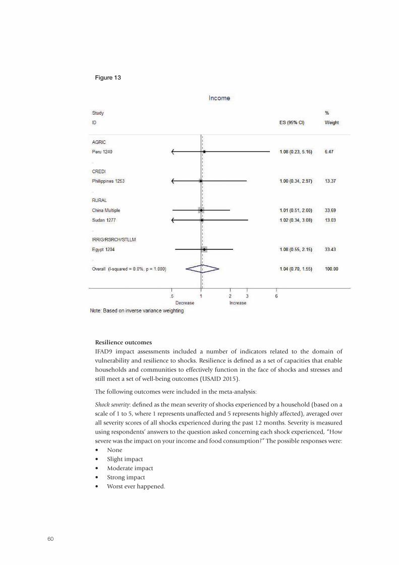
60
Resilience outcomesIFAD9 impact assessments included a number of indicators related to the domain of
vulnerability and resilience to shocks. Resilience is defined as a set of capacities that enable
households and communities to effectively function in the face of shocks and stresses and
still meet a set of well-being outcomes (USAID 2015).
The following outcomes were included in the meta-analysis:
Shock severity: defined as the mean severity of shocks experienced by a household (based on a
scale of 1 to 5, where 1 represents unaffected and 5 represents highly affected), averaged over
all severity scores of all shocks experienced during the past 12 months. Severity is measured
using respondents’ answers to the question asked concerning each shock experienced, “How
severe was the impact on your income and food consumption?” The possible responses were:
• None
• Slight impact
• Moderate impact
• Strong impact
• Worst ever happened.
Figure 13
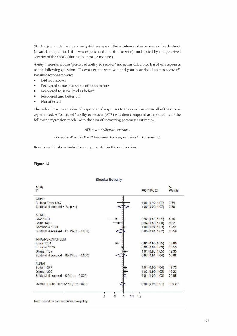
61
Shock exposure: defined as a weighted average of the incidence of experience of each shock (a variable equal to 1 if it was experienced and 0 otherwise), multiplied by the perceived severity of the shock (during the past 12 months).
Ability to recover: a base “perceived ability to recover” index was calculated based on responses to the following question: “To what extent were you and your household able to recover?” Possible responses were:• Did not recover• Recovered some, but worse off than before• Recovered to same level as before• Recovered and better off• Not affected.
The index is the mean value of respondents’ responses to the question across all of the shocks experienced. A “corrected” ability to recover (ATR) was then computed as an outcome to the following regression model with the aim of recovering parameter estimates:
ATR = ∝ + β*Shocks exposure.
Corrected ATR = ATR + β* (average shock exposure – shock exposure).
Results on the above indicators are presented in the next section.
Figure 14
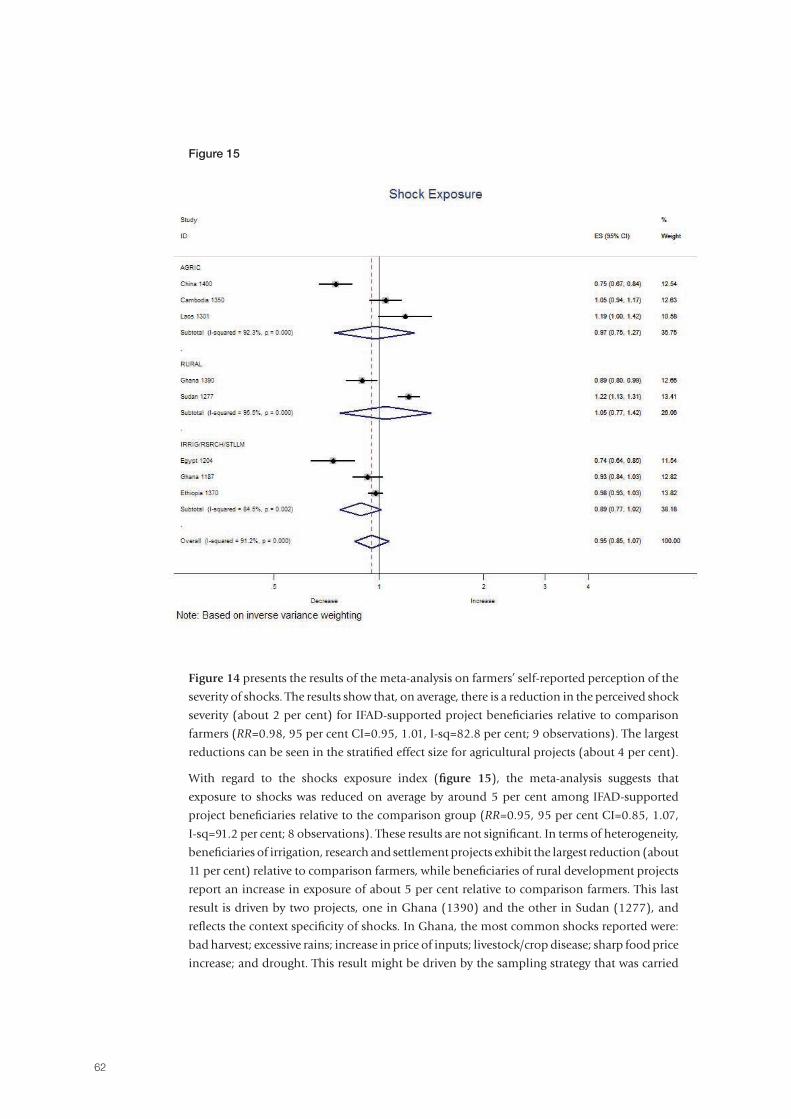
62
Figure 14 presents the results of the meta-analysis on farmers’ self-reported perception of the
severity of shocks. The results show that, on average, there is a reduction in the perceived shock
severity (about 2 per cent) for IFAD-supported project beneficiaries relative to comparison
farmers (RR=0.98, 95 per cent CI=0.95, 1.01, I-sq=82.8 per cent; 9 observations). The largest
reductions can be seen in the stratified effect size for agricultural projects (about 4 per cent).
With regard to the shocks exposure index (figure 15), the meta-analysis suggests that
exposure to shocks was reduced on average by around 5 per cent among IFAD-supported
project beneficiaries relative to the comparison group (RR=0.95, 95 per cent CI=0.85, 1.07,
I-sq=91.2 per cent; 8 observations). These results are not significant. In terms of heterogeneity,
beneficiaries of irrigation, research and settlement projects exhibit the largest reduction (about
11 per cent) relative to comparison farmers, while beneficiaries of rural development projects
report an increase in exposure of about 5 per cent relative to comparison farmers. This last
result is driven by two projects, one in Ghana (1390) and the other in Sudan (1277), and
reflects the context specificity of shocks. In Ghana, the most common shocks reported were:
bad harvest; excessive rains; increase in price of inputs; livestock/crop disease; sharp food price
increase; and drought. This result might be driven by the sampling strategy that was carried
Figure 15
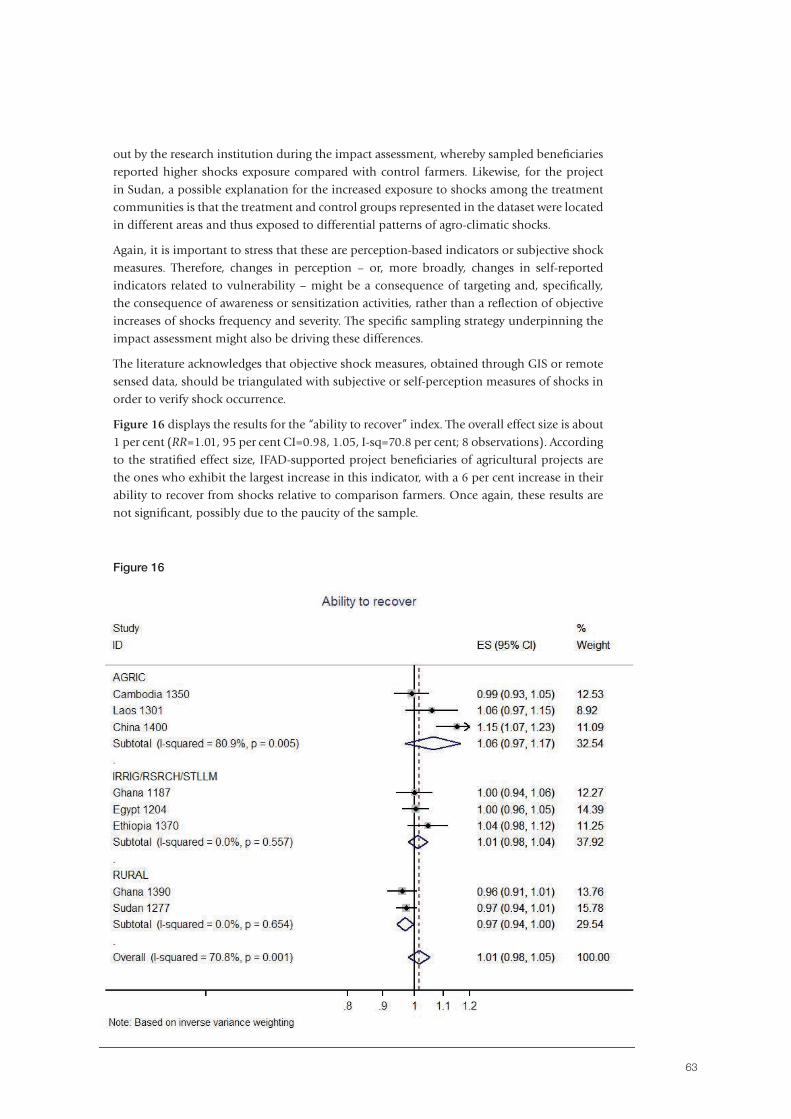
63
out by the research institution during the impact assessment, whereby sampled beneficiaries reported higher shocks exposure compared with control farmers. Likewise, for the project in Sudan, a possible explanation for the increased exposure to shocks among the treatment communities is that the treatment and control groups represented in the dataset were located in different areas and thus exposed to differential patterns of agro-climatic shocks.
Again, it is important to stress that these are perception-based indicators or subjective shock measures. Therefore, changes in perception – or, more broadly, changes in self-reported indicators related to vulnerability – might be a consequence of targeting and, specifically, the consequence of awareness or sensitization activities, rather than a reflection of objective increases of shocks frequency and severity. The specific sampling strategy underpinning the impact assessment might also be driving these differences.
The literature acknowledges that objective shock measures, obtained through GIS or remote sensed data, should be triangulated with subjective or self-perception measures of shocks in order to verify shock occurrence.
Figure 16 displays the results for the “ability to recover” index. The overall effect size is about 1 per cent (RR=1.01, 95 per cent CI=0.98, 1.05, I-sq=70.8 per cent; 8 observations). According to the stratified effect size, IFAD-supported project beneficiaries of agricultural projects are the ones who exhibit the largest increase in this indicator, with a 6 per cent increase in their ability to recover from shocks relative to comparison farmers. Once again, these results are not significant, possibly due to the paucity of the sample.
Figure 16
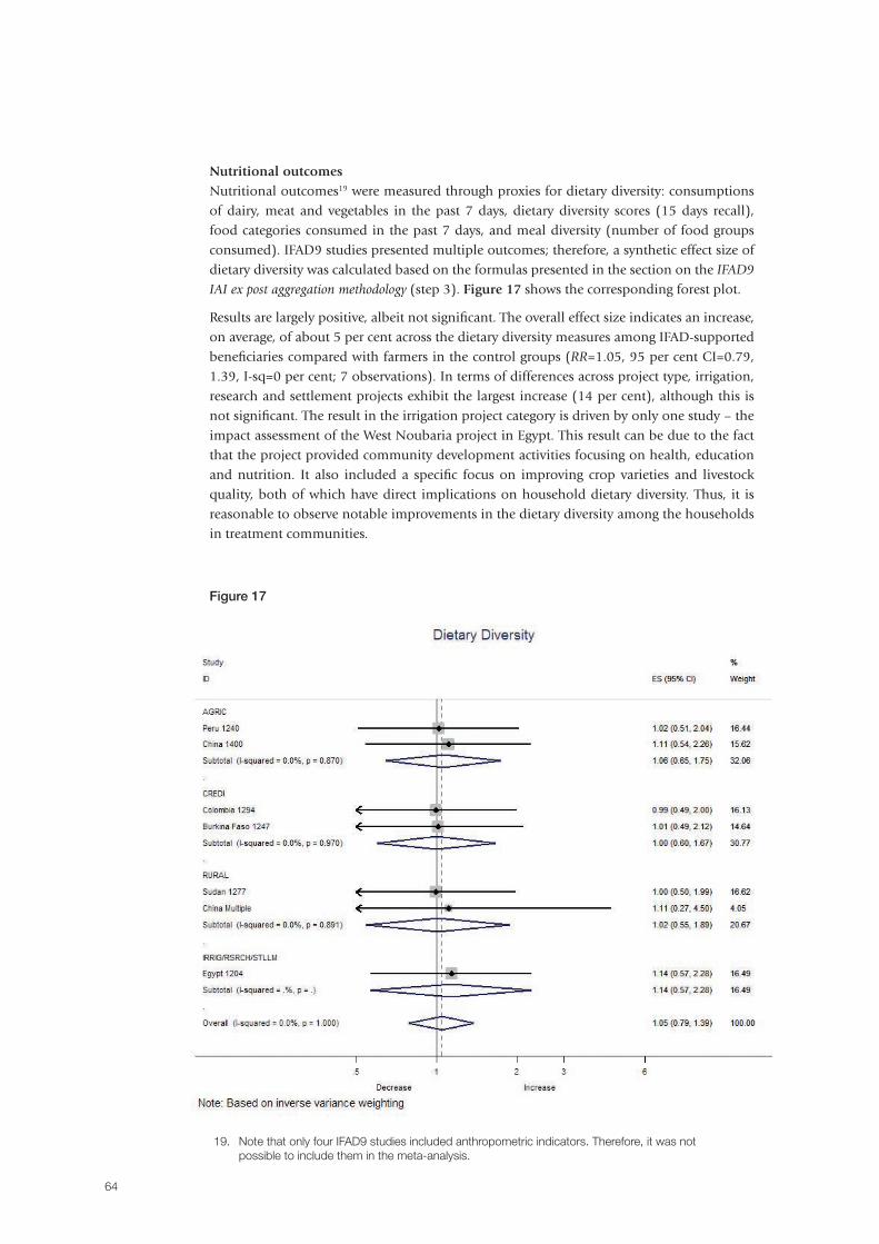
64
Nutritional outcomesNutritional outcomes19 were measured through proxies for dietary diversity: consumptions of dairy, meat and vegetables in the past 7 days, dietary diversity scores (15 days recall), food categories consumed in the past 7 days, and meal diversity (number of food groups consumed). IFAD9 studies presented multiple outcomes; therefore, a synthetic effect size of dietary diversity was calculated based on the formulas presented in the section on the IFAD9
IAI ex post aggregation methodology (step 3). Figure 17 shows the corresponding forest plot.
Results are largely positive, albeit not significant. The overall effect size indicates an increase, on average, of about 5 per cent across the dietary diversity measures among IFAD-supported beneficiaries compared with farmers in the control groups (RR=1.05, 95 per cent CI=0.79, 1.39, I-sq=0 per cent; 7 observations). In terms of differences across project type, irrigation, research and settlement projects exhibit the largest increase (14 per cent), although this is not significant. The result in the irrigation project category is driven by only one study – the impact assessment of the West Noubaria project in Egypt. This result can be due to the fact that the project provided community development activities focusing on health, education and nutrition. It also included a specific focus on improving crop varieties and livestock quality, both of which have direct implications on household dietary diversity. Thus, it is reasonable to observe notable improvements in the dietary diversity among the households in treatment communities.
19. Note that only four IFAD9 studies included anthropometric indicators. Therefore, it was not possible to include them in the meta-analysis.
Figure 17
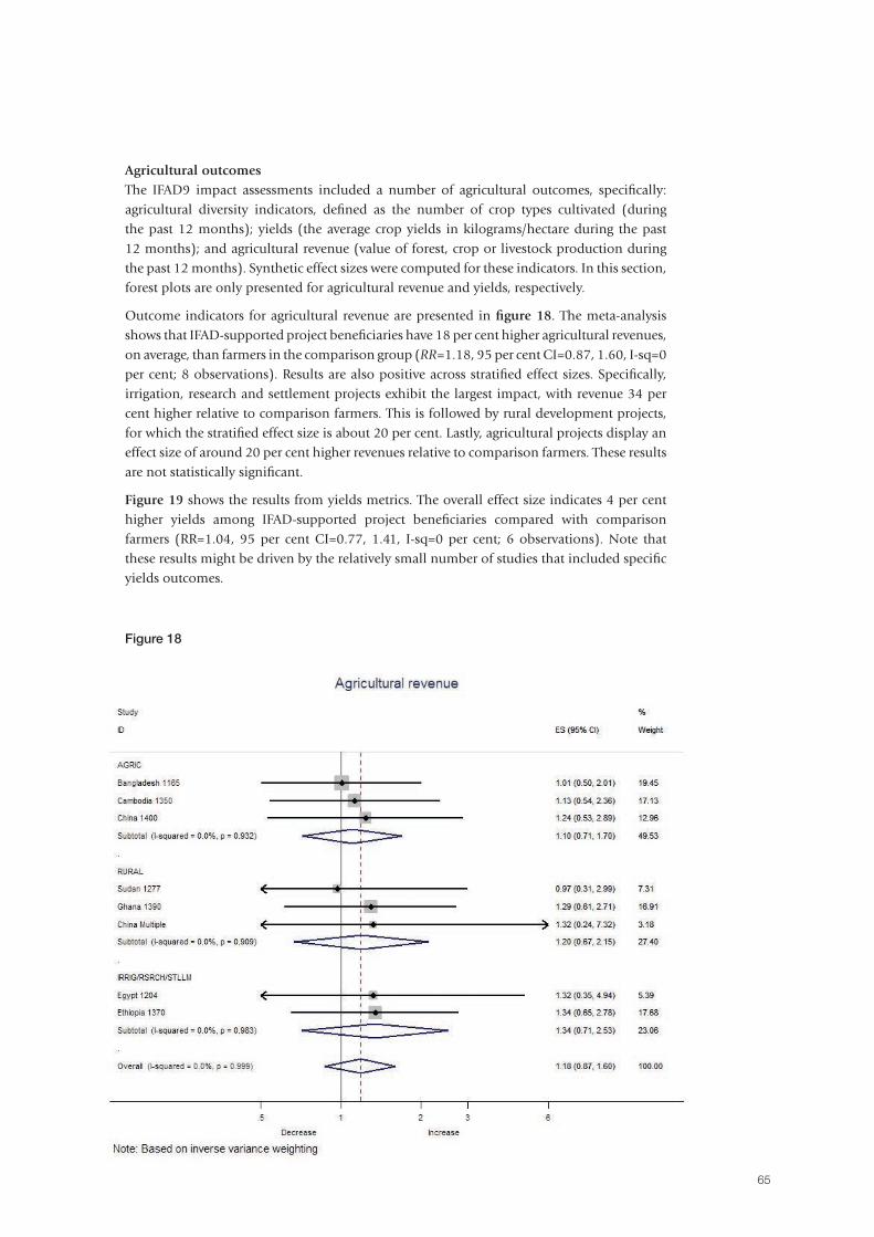
65
Agricultural outcomesThe IFAD9 impact assessments included a number of agricultural outcomes, specifically: agricultural diversity indicators, defined as the number of crop types cultivated (during the past 12 months); yields (the average crop yields in kilograms/hectare during the past 12 months); and agricultural revenue (value of forest, crop or livestock production during the past 12 months). Synthetic effect sizes were computed for these indicators. In this section, forest plots are only presented for agricultural revenue and yields, respectively.
Outcome indicators for agricultural revenue are presented in figure 18. The meta-analysis shows that IFAD-supported project beneficiaries have 18 per cent higher agricultural revenues, on average, than farmers in the comparison group (RR=1.18, 95 per cent CI=0.87, 1.60, I-sq=0 per cent; 8 observations). Results are also positive across stratified effect sizes. Specifically, irrigation, research and settlement projects exhibit the largest impact, with revenue 34 per cent higher relative to comparison farmers. This is followed by rural development projects, for which the stratified effect size is about 20 per cent. Lastly, agricultural projects display an effect size of around 20 per cent higher revenues relative to comparison farmers. These results are not statistically significant.
Figure 19 shows the results from yields metrics. The overall effect size indicates 4 per cent higher yields among IFAD-supported project beneficiaries compared with comparison farmers (RR=1.04, 95 per cent CI=0.77, 1.41, I-sq=0 per cent; 6 observations). Note that these results might be driven by the relatively small number of studies that included specific yields outcomes.
Figure 18
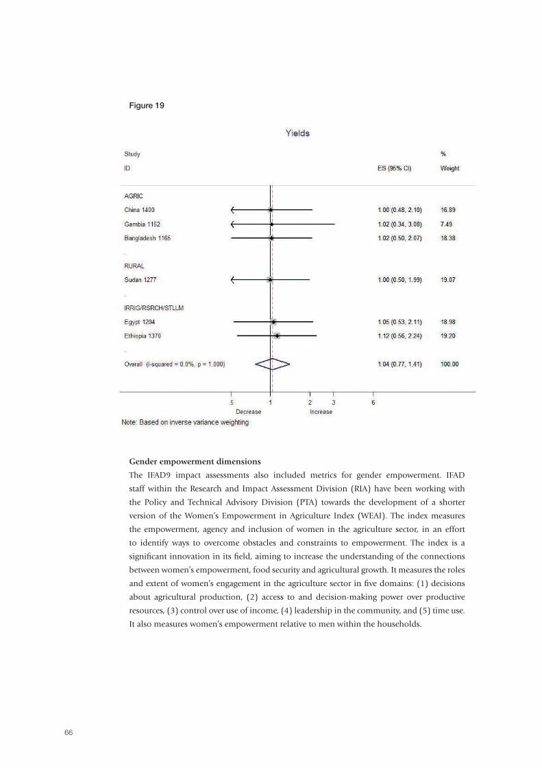
66
Figure 19
Gender empowerment dimensions
The IFAD9 impact assessments also included metrics for gender empowerment. IFAD
staff within the Research and Impact Assessment Division (RIA) have been working with
the Policy and Technical Advisory Division (PTA) towards the development of a shorter
version of the Women’s Empowerment in Agriculture Index (WEAI). The index measures
the empowerment, agency and inclusion of women in the agriculture sector, in an effort
to identify ways to overcome obstacles and constraints to empowerment. The index is a
significant innovation in its field, aiming to increase the understanding of the connections
between women’s empowerment, food security and agricultural growth. It measures the roles
and extent of women’s engagement in the agriculture sector in five domains: (1) decisions
about agricultural production, (2) access to and decision-making power over productive
resources, (3) control over use of income, (4) leadership in the community, and (5) time use.
It also measures women’s empowerment relative to men within the households.
67
Using MCA and datasets from Bangladesh, Guatemala and Uganda, IFAD developed a shorter
version for measuring empowerment that reduces the number of original dimensions within
the index, as well as the number of questions within each dimension.20
As the administration of a gender module requires dual interviews (involving both husband
and wife), survey costs were effectively doubled. Therefore, IFAD recommended the addition
of a gender empowerment module after examining the relevance of the indicator within the
project specific theory of change.
In addition, partners fielding the data collection felt that a few questions would adequately
capture gender outcomes, or had mixed views about the WEAI in general and felt that other
indexes – such as the Schneider Gender Index – could perform better (such was the case for
the study in Pakistan). Some of the Deep Dives employed existing datasets, where gender
empowerment proxies were not collected.
In order to maximize the use of available indicators, and since it was not possible to compute
the WEAI (even in its reduced form) for all datasets due to the lack of the necessary variables,
the IFAD staff decided to group the gender outcomes in three domains, namely participation,
access and control over resources, and compute synthetic effect size through the meta-analysis.
The gender participation outcomes included: outcomes related to economic activity and
community group involvement; access/ownership-related outcomes that covered education
and literacy level, as well as sole or joint ownership of livestock and land; and control-related
outcomes that included involvement in decision-making around business and household
expenditures, economic activities and borrowing.
Since low- and medium-bias studies did not have the three domains at the same time
(apart from the study in Bangladesh [1165]), all available outcomes were meta-analysed
and the following effect sizes were obtained. Of all the studies considered in this exercise,
six included measures within the gender control domain, one study included access, and
five included participation.
Figure 20 presents results that meta-analyse the various gender dimensions (access,
participation, and control). Note that each of the study-specific effect sizes is a synthetic effect
size, as there were different measures of access, participation and control within each study.
The overall effect size indicates that, on average, results were largely positive, although not
significant; beneficiaries exhibited 5 per cent higher gender empowerment outcomes compared
with control farmers (RR=1.18, 95 per cent CI=0.87, 1.60, I-sq=0 per cent; 8 observations).
Agricultural projects were the ones that drove the overall effect size calculation, with the
study in Bangladesh (1165) presenting the largest impacts in terms of empowerment metrics,
along with the studies in China (1400) and Ghana (1390, 1187).
The study in Bangladesh (1165) evaluated the project’s fishery component. The interventions
aimed to provide poor fishers with access to beels (water bodies) and introduced the Beel User
Groups (BUGs), which enabled women to gain access to fishing opportunities and also to
engage in the management of the BUGs, leading to increased income generated from fishing.
20. See the IFAD9 Impact Assessment questionnaire in the IFAD9 Sourcebook for the specific section on measuring gender empowerment with a “reduced-form” WEAI (Garbero 2014b).
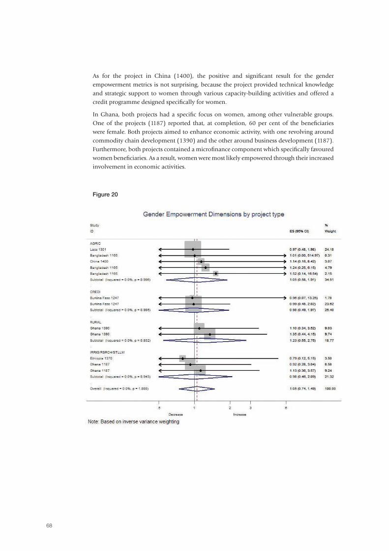
68
As for the project in China (1400), the positive and significant result for the gender empowerment metrics is not surprising, because the project provided technical knowledge and strategic support to women through various capacity-building activities and offered a credit programme designed specifically for women.
In Ghana, both projects had a specific focus on women, among other vulnerable groups. One of the projects (1187) reported that, at completion, 60 per cent of the beneficiaries were female. Both projects aimed to enhance economic activity, with one revolving around commodity chain development (1390) and the other around business development (1187). Furthermore, both projects contained a microfinance component which specifically favoured women beneficiaries. As a result, women were most likely empowered through their increased involvement in economic activities.
Figure 20
69
Poverty outcomes While recognizing the limitations of a “movement out of poverty” measure as articulated previously, poverty reduction impacts have been estimated using an assets-based approach applied to individual surveys. While income data were collected in a few studies, they were insufficient and not suitable for the computation of poverty dynamics. In contrast, asset-based poverty measures were widely available and deemed of higher quality, since their collection is more straightforward and less prone to measurement error, particularly when using recall methods. As indicated in the updates on the methodology,21 relative poverty lines were employed and defined using the 40th and 60th percentile22 cut-offs of the corresponding asset index distribution of the control group, as the latter represented the counterfactual, i.e. the reference point (IFAD 2015a).
Binary indicators (indicating poverty status at endline, defined according to the specific percentile cut-off) were constructed from the continuous distributions of the various asset indices. Such indicators were meta-analysed and produced the aggregate poverty reduction estimates that are presented in the following figures. Note that, in this section, poverty reduction impacts are presented using a number of asset-based proxies and two poverty lines. Recall that poverty proxies based on assets indicators including only durables are considered the preferred proxies on the grounds that they better approximate long-run wealth, in addition to being widely available for all IFAD9 ex post studies.
Figure 21 presents poverty reduction estimates using a 40th percentile poverty line. Using the durable assets index as the asset-based welfare proxy, poverty reduction impacts are estimated to be around 5.6 per cent; in other words, IFAD-supported project beneficiaries are, on average, 6 per cent more likely to be above the poverty line than comparison beneficiaries at endline. Note that this finding is not statistically significant at 5 per cent level, as the 95 per cent confidence interval includes 1.00, i.e. the point of no effect (RR=1.06, 95 per cent CI=1.00, 1.11, I-sq=93 per cent; 18 observations). However, although the overall effect is not significant, results present a substantial degree of heterogeneity by project type. Irrigation projects exhibit the highest poverty reduction impacts, whereby beneficiaries are 24 per cent more likely to be above the poverty line than comparison farmers (this is statistically significant at 5 per cent level). Credit projects are next, with a 10 per cent significant impact, while agricultural projects present a poverty reduction impact of only 2 per cent (albeit not significant). Rural development projects reduce the portion of those above the poverty line by 3 per cent (implying that 3 per cent move into poverty), although this finding is also not statistically significant.
21. See An update on the methodology for estimating the number of people moved out of poverty and preparatory work for the impact assessment exercise during IFAD10 (EB 2015/114/INF.3).
22. To check whether results would differ if an income-based poverty line was used, an analysis of poverty dynamics was completed for four countries for which income data and a national poverty line was available: in two cases, results were similar; in one case, the poverty impact was estimated as higher; and in one case, the estimate was lower. This is not surprising, given results are likely to change based on where a line is placed. Overall, the expectation is that an income-based poverty line would end up with a similar aggregate impact. Please see the details in the section on the Sensitivity analysis to different poverty lines in the Appendices.
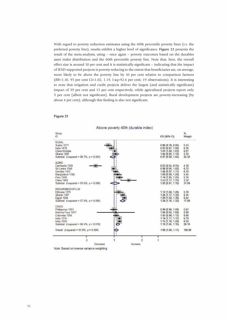
70
With regard to poverty reduction estimates using the 60th percentile poverty lines (i.e. the preferred poverty line), results exhibit a higher level of significance. Figure 22 presents the result of the meta-analysis, using – once again – poverty outcomes based on the durables asset index distribution and the 60th percentile poverty line. Note that, here, the overall effect size is around 10 per cent and it is statistically significant – indicating that the impact of IFAD-supported projects is poverty reducing to the extent that beneficiaries are, on average, more likely to be above the poverty line by 10 per cent relative to comparison farmers (RR=1.10, 95 per cent CI=1.02, 1.19, I-sq=92.6 per cent; 19 observations). It is interesting to note that irrigation and credit projects deliver the largest (and statistically significant) impact of 39 per cent and 15 per cent respectively, while agricultural projects report only 5 per cent (albeit not significant). Rural development projects are poverty-increasing (by about 4 per cent), although this finding is also not significant.
Figure 21
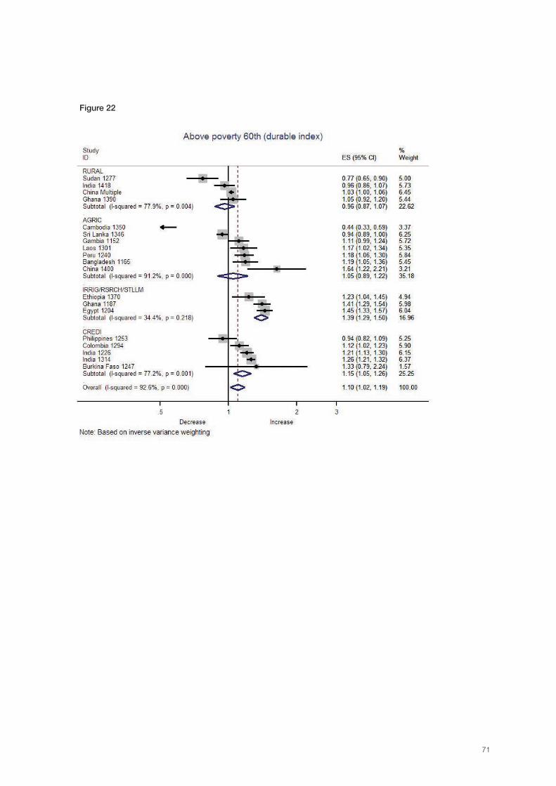
71
Figure 22
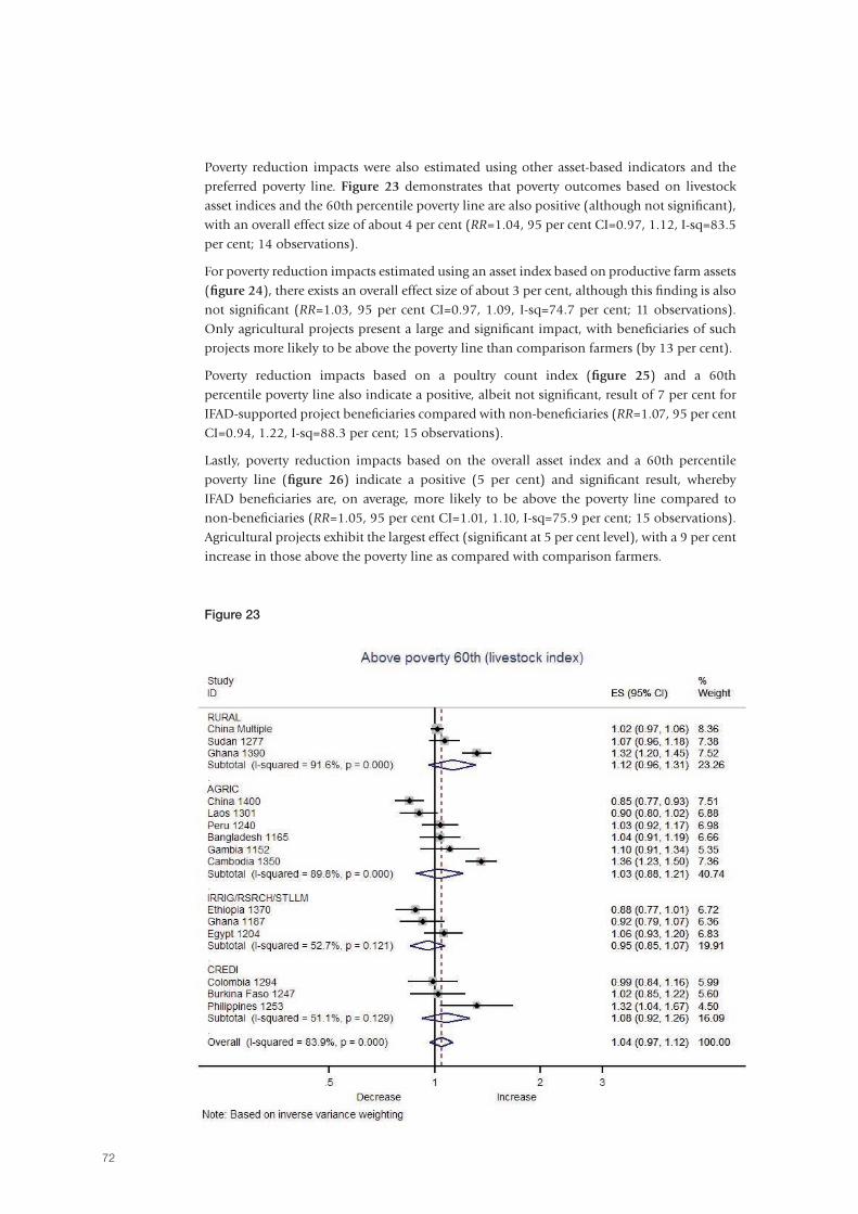
72
Poverty reduction impacts were also estimated using other asset-based indicators and the preferred poverty line. Figure 23 demonstrates that poverty outcomes based on livestock asset indices and the 60th percentile poverty line are also positive (although not significant), with an overall effect size of about 4 per cent (RR=1.04, 95 per cent CI=0.97, 1.12, I-sq=83.5 per cent; 14 observations).
For poverty reduction impacts estimated using an asset index based on productive farm assets (figure 24), there exists an overall effect size of about 3 per cent, although this finding is also not significant (RR=1.03, 95 per cent CI=0.97, 1.09, I-sq=74.7 per cent; 11 observations). Only agricultural projects present a large and significant impact, with beneficiaries of such projects more likely to be above the poverty line than comparison farmers (by 13 per cent).
Poverty reduction impacts based on a poultry count index (figure 25) and a 60th percentile poverty line also indicate a positive, albeit not significant, result of 7 per cent for IFAD-supported project beneficiaries compared with non-beneficiaries (RR=1.07, 95 per cent CI=0.94, 1.22, I-sq=88.3 per cent; 15 observations).
Lastly, poverty reduction impacts based on the overall asset index and a 60th percentile poverty line (figure 26) indicate a positive (5 per cent) and significant result, whereby IFAD beneficiaries are, on average, more likely to be above the poverty line compared to non-beneficiaries (RR=1.05, 95 per cent CI=1.01, 1.10, I-sq=75.9 per cent; 15 observations). Agricultural projects exhibit the largest effect (significant at 5 per cent level), with a 9 per cent increase in those above the poverty line as compared with comparison farmers.
Figure 23
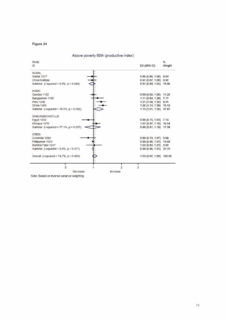
73
Figure 24
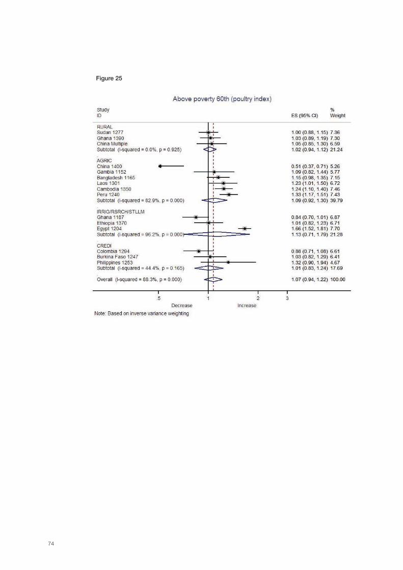
74
Figure 25
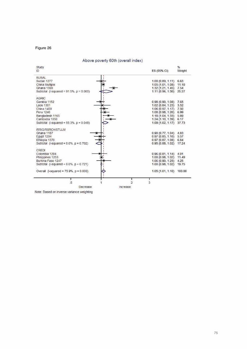
75
Figure 26

76
SummaryIn summary, the results from the meta-analysis show that there are many areas in which IFAD-supported project beneficiaries have, on average, better outcomes in percentage terms as compared with the control group. Assessing impact requires identifying whether, on average, IFAD beneficiaries are better off than they would be in the absence of an IFAD project – that is, obtaining the difference between treatment and comparison farmers. The results show that IFAD-supported projects are effectively poverty-reducing: when choosing durable asset indexes as the preferred poverty proxy on the grounds that it better approximates long-run wealth, findings point to statistically significant gains, particularly for irrigation and credit projects. This finding is sensitive to the choice of the poverty line.
The positive results for each poverty measure suggest that there is a general increase in assets similar to the shifting distribution noted in figure 2 and those highlighted for individual countries in figure 8. Using the methodology described in the previous sections, IFAD investments are projected to reduce poverty by between 5.6 per cent and 9.9 per cent using the 40th and 60th percentile cut-offs of the durable assets distribution. The generally lower estimates for the 40th percentile line suggest that project impacts are concentrated in the middle of the distribution. The lower results for productive-, livestock- and poultry-defined asset indicators highlight the greater narrowness of their definitions. Note that the lower results obtained while using an overall asset index as the poverty proxy are due to the fact that the latter comprises the three indices and may thus include entities that offset one another.
When considering the entire income distribution of IFAD-supported beneficiaries, the results indicate that IFAD9 projects increase the economic mobility of recipients by significantly increasing assets and expenditures. Projects are also building resilience, improving nutrition and expanding agricultural production and livestock ownership. Many beneficiaries of
IFAD-supported projects are significantly increasing their livestock holdings. Irrigation, research and settlement projects are dramatically reducing poverty, augmenting agricultural revenues and improving dietary diversity, while reducing exposure to shocks. Agricultural development programmes are significantly expanding farmers’ wealth in terms of productive farm assets and small livestock ownership. Results for rural development projects are large and positive, but not statistically significant, and include outcomes such as poultry ownership, agricultural diversity and revenue, which contribute to the empowerment of women.
One can conclude that, overall, the analysis strongly implies that IFAD is effectively improving the well-being of rural people in terms of asset accumulation and higher revenue and income.
Table 5 summarizes the estimated effect sizes, described in detail in the previous section, by impact domain and outcome.
Table 6 summarizes estimated impacts in percentage terms for ease of interpretation. Results highlighted indicate statistical significance at 5 per cent level.
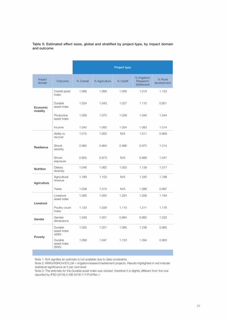
77
Project type
Impact domain Outcome % Overall % Agriculture % Credit
% Irrigation/ Research/ Settlement
% Rural development
Economic mobility
Overall asset index
1.066 1.066 1.056 1.019 1.133
Durable asset index
1.034 1.043 1.027 1.110 0.951
Productive asset index
1.056 1.075 1.038 1.040 1.044
Income 1.040 1.083 1.004 1.083 1.014
Resilience
Ability to recover
1.015 1.063 N/A 1.011 0.969
Shock severity
0.982 0.964 0.996 0.972 1.014
Shock exposure
0.955 0.973 N/A 0.889 1.047
Nutrition Dietary diversity
1.046 1.062 1.003 1.139 1.017
Agriculture
Agricultural revenue
1.180 1.103 N/A 1.340 1.198
Yields 1.038 1.015 N/A 1.088 0.997
Livestock
Livestock asset index
1.095 1.055 1.254 1.026 1.194
Poultry count index
1.120 1.039 1.110 1.211 1.176
GenderGender dimensions
1.048 1.051 0.984 0.982 1.225
Poverty
Durable asset index (40th)
1.055 1.021 1.095 1.236 0.965
Durable asset index (60th)
1.099 1.047 1.153 1.394 0.963
Table 5: Estimated effect sizes, global and stratified by project-type, by impact domain and outcome
Note 1: N/A signifies an estimate is not available due to data constraints.Note 2: IRRIG/RSRCH/STLLM = irrigation/research/settlement projects. Results highlighted in red indicate statistical significance at 5 per cent level. Note 3: The estimate for the Durable asset index was revised, therefore it is slightly different from the one reported by IFAD (2016) in EB 2016/117/R.8/Rev.1.
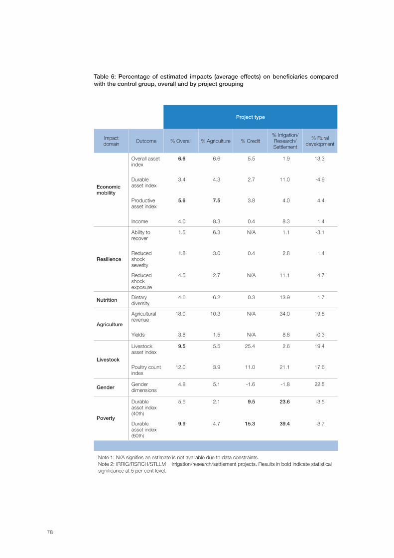
78
Project type
Impact domain Outcome % Overall % Agriculture % Credit
% Irrigation/ Research/ Settlement
% Rural development
Economic mobility
Overall asset index
6.6 6.6 5.5 1.9 13.3
Durable asset index
3.4 4.3 2.7 11.0 -4.9
Productive asset index
5.6 7.5 3.8 4.0 4.4
Income 4.0 8.3 0.4 8.3 1.4
Resilience
Ability to recover
1.5 6.3 N/A 1.1 -3.1
Reduced shock severity
1.8 3.0 0.4 2.8 1.4
Reduced shock exposure
4.5 2.7 N/A 11.1 4.7
Nutrition Dietary diversity
4.6 6.2 0.3 13.9 1.7
Agriculture
Agricultural revenue
18.0 10.3 N/A 34.0 19.8
Yields 3.8 1.5 N/A 8.8 -0.3
Livestock
Livestock asset index
9.5 5.5 25.4 2.6 19.4
Poultry count index
12.0 3.9 11.0 21.1 17.6
GenderGender dimensions
4.8 5.1 -1.6 -1.8 22.5
Poverty
Durable asset index (40th)
5.5 2.1 9.5 23.6 -3.5
Durable asset index (60th)
9.9 4.7 15.3 39.4 -3.7
Table 6: Percentage of estimated impacts (average effects) on beneficiaries compared with the control group, overall and by project grouping
Note 1: N/A signifies an estimate is not available due to data constraints.Note 2: IRRIG/RSRCH/STLLM = irrigation/research/settlement projects. Results in bold indicate statistical significance at 5 per cent level.
79
Results from the IFAD9 projections
The results presented in the previous section are the average effects, and represent the
estimated impact on the recipients as compared with the control group. Actual impacts on
individual beneficiaries will vary, with some receiving greater benefits than the average and
others receiving less. Precisely calculating those who benefit is not possible given the available
data and requires making some assumptions about the amount of benefit. A conservative
estimate is to assume a doubling of benefits for some and zero for the remaining population
– and extrapolating this to the projected population of beneficiaries.
In this section, the impact projections are presented. Note that the projection universe refers
to an overall population of expected direct and indirect beneficiaries for the whole portfolio
of projects closed and ongoing during the period 2010-2015, which amounts to around
390 projects with a total of about 240 million projected beneficiaries. Of course, this number
differs from the estimates of actual beneficiaries currently receiving services from the same
projects (139 million, as reported in table 2), as these are calculated up to a certain point in
time (end-2014) and only for the projects that have initiated activities on the ground.
Figure 27 shows the results from the projections using a wide set of indicators.
When impact estimates are applied to IFAD projects, the resultant projections indicate that
43.2 million beneficiaries exhibited a significant and substantial increase in their agricultural
revenue; 28.8 million – a rise in poultry ownership; and 22.8 million – an increase in livestock
assets. With regard to overall assets, productive assets, gender empowerment, dietary diversity
and reduction in shock exposure, the evidence shows that over 10 million beneficiaries felt
substantial gains in these areas. Of course, there is some overlap of benefits, whereby some
individuals have received multiple benefits, both in terms of impacts noted in figure 27as well
as impacts that were not measurable. Overall, the results suggest that benefits are substantial
and widespread, with a high likelihood that nearly all projected recipients will receive at least
some form of benefit. They clearly show that IFAD’s investment in rural people is leading to
substantial returns by helping millions of rural people improve their livelihoods.
As far as the projections of poverty dynamics are concerned, aggregate results show that
when using a durable asset index as an underlying poverty proxy, projected impacts
enable 23.8 million beneficiaries to move from below to above the relative 60th percentile
poverty line. Note that this finding is statistically significant at the 5 per cent level and
corresponds to a net poverty reduction impact of 9.9 per cent, which can be attributed to IFAD-supported projects.
The results highlight how projections are sensitive to underlying assumptions and can
significantly vary depending on how the poverty line is defined. Furthermore, the projections
reinforce the notion that focusing on a single narrow and discrete measure does not
adequately reflect the returns to IFAD investments. It suggests the endorsement of the notion
that the latter should be assessed more widely using a comprehensive set of indicators that
capture adequately the project-specific theory of change.
Finally, note that these projections represent a “what if” and lower-bound scenario, and cannot
clearly indicate if IFAD has reached a given target, since they assume that previous projects
have similar characteristics and are good predictors for current and future projects. Clearly,
this is not the case and such an assumption potentially underestimates the poverty reduction
impact, as IFAD has already shifted its emphasis with regard to portfolio characteristics and
seeks to further improve its development effectiveness.
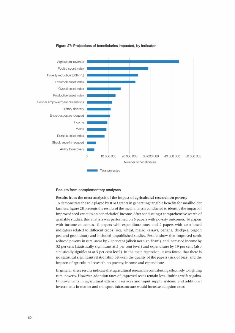
80
Results from complementary analyses
Results from the meta-analysis of the impact of agricultural research on poverty
To demonstrate the role played by IFAD grants in generating tangible benefits for smallholder
farmers, figure 28 presents the results of the meta-analysis conducted to identify the impact of
improved seed varieties on beneficiaries’ income. After conducting a comprehensive search of
available studies, this analysis was performed on 6 papers with poverty outcomes, 16 papers
with income outcomes, 11 papers with expenditure ones and 2 papers with asset-based
indicators related to different crops (rice, wheat, maize, cassava, banana, chickpea, pigeon
pea and groundnut) and included unpublished studies. Results show that improved seeds
reduced poverty in rural areas by 20 per cent (albeit not significant), and increased income by
32 per cent (statistically significant at 5 per cent level) and expenditure by 19 per cent (also
statistically significant at 5 per cent level). In the meta-regression, it was found that there is
no statistical significant relationship between the quality of the papers (risk of bias) and the
impacts of agricultural research on poverty, income and expenditure.
In general, these results indicate that agricultural research is contributing effectively to fighting
rural poverty. However, adoption rates of improved seeds remain low, limiting welfare gains.
Improvements in agricultural extension services and input supply systems, and additional
investments in market and transport infrastructure would increase adoption rates.
Figure 27: Projections of beneficiaries impacted, by indicator
Agricultural revenue
Poultry count index
Poverty reduction (60th PL)
Livestock asset index
Overall asset index
Productive asset index
Gender empowerment dimensions
Dietary diversity
Shock exposure reduced
Income
Yields
Durable asset index
Shock severity reduced
Ability to recovery
0 10 000 000 20 000 000 30 000 000 40 000 000 50 000 000
Number of beneficiaries
Total projected
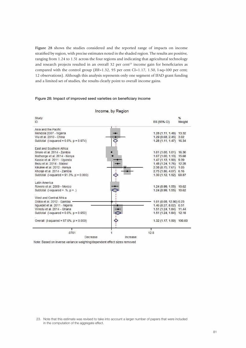
81
Figure 28 shows the studies considered and the reported range of impacts on income stratified by region, with precise estimates noted in the shaded region. The results are positive, ranging from 1.24 to 1.51 across the four regions and indicating that agricultural technology and research projects resulted in an overall 32 per cent23 income gain for beneficiaries as compared with the control group (RR=1.32, 95 per cent CI=1.17, 1.50, I-sq=100 per cent; 12 observations). Although this analysis represents only one segment of IFAD grant funding and a limited set of studies, the results clearly point to overall income gains.
23. Note that this estimate was revised to take into account a larger number of papers that were included in the computation of the aggregate effect.
Figure 28: Impact of improved seed varieties on beneficiary income
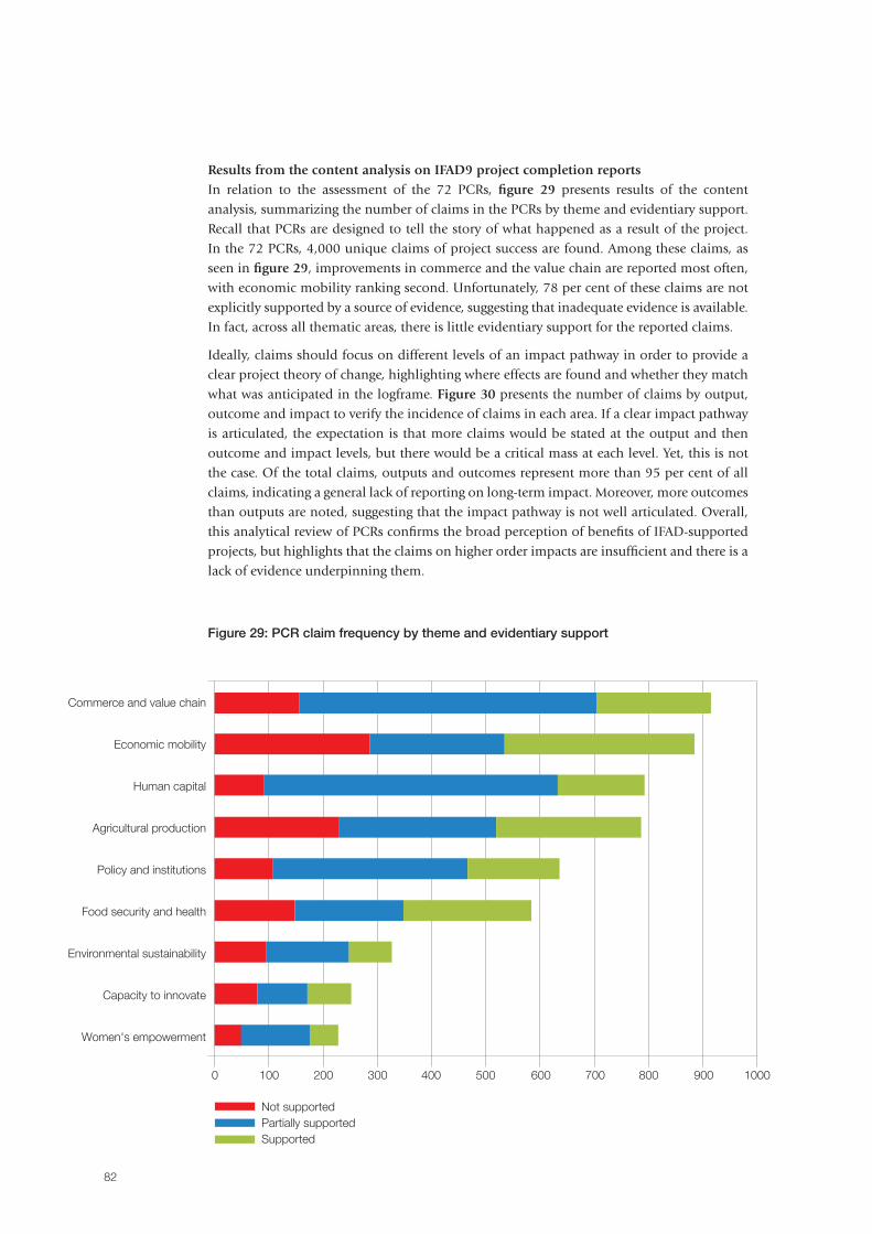
82
Results from the content analysis on IFAD9 project completion reportsIn relation to the assessment of the 72 PCRs, figure 29 presents results of the content
analysis, summarizing the number of claims in the PCRs by theme and evidentiary support.
Recall that PCRs are designed to tell the story of what happened as a result of the project.
In the 72 PCRs, 4,000 unique claims of project success are found. Among these claims, as
seen in figure 29, improvements in commerce and the value chain are reported most often,
with economic mobility ranking second. Unfortunately, 78 per cent of these claims are not
explicitly supported by a source of evidence, suggesting that inadequate evidence is available.
In fact, across all thematic areas, there is little evidentiary support for the reported claims.
Ideally, claims should focus on different levels of an impact pathway in order to provide a
clear project theory of change, highlighting where effects are found and whether they match
what was anticipated in the logframe. Figure 30 presents the number of claims by output,
outcome and impact to verify the incidence of claims in each area. If a clear impact pathway
is articulated, the expectation is that more claims would be stated at the output and then
outcome and impact levels, but there would be a critical mass at each level. Yet, this is not
the case. Of the total claims, outputs and outcomes represent more than 95 per cent of all
claims, indicating a general lack of reporting on long-term impact. Moreover, more outcomes
than outputs are noted, suggesting that the impact pathway is not well articulated. Overall,
this analytical review of PCRs confirms the broad perception of benefits of IFAD-supported
projects, but highlights that the claims on higher order impacts are insufficient and there is a
lack of evidence underpinning them.
Figure 29: PCR claim frequency by theme and evidentiary support
0 100 200 300 400 500 600 700 800 900 1000
Commerce and value chain
Economic mobility
Human capital
Agricultural production
Policy and institutions
Food security and health
Environmental sustainability
Capacity to innovate
Women's empowerment
Not supportedPartially supportedSupported
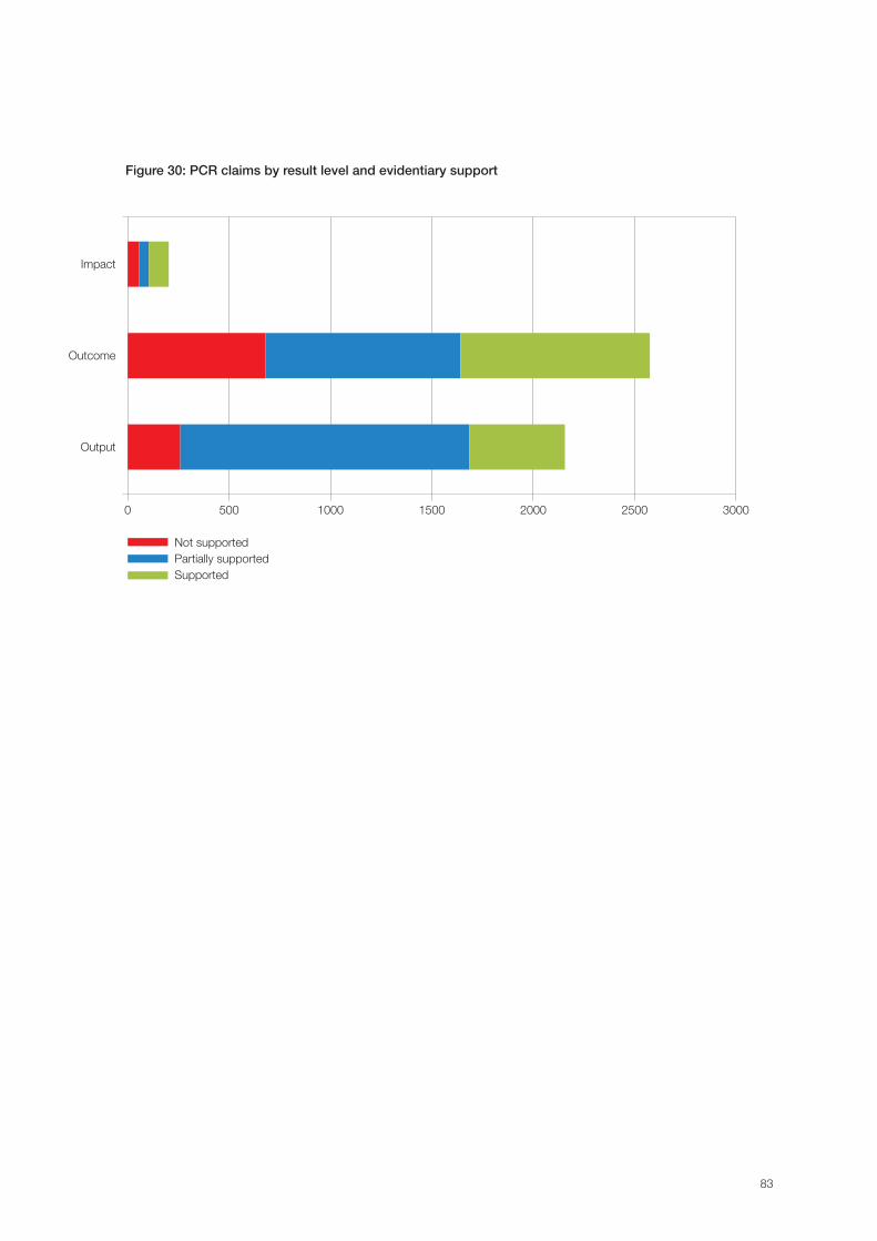
83
Figure 30: PCR claims by result level and evidentiary support
Impact
Outcome
Output
Not supportedPartially supportedSupported
0 500 1000 1500 2000 2500 3000
84
The IFAD9 IAI has provided IFAD with significant lessons that will help advance a results-based
agenda. On methods, the IFAD9 IAI represents a pioneering effort in trying to overcome the
clear challenges of designing data collection and conducting impact assessments ex post.
The initiative draws attention to the fact that using a representative sample of projects and
focusing on one aggregate indicator limits the potential for learning and is unnecessarily
restrictive – projects should be identified where learning will be the greatest, and indicators
need to be selected to comprehensively represent IFAD’s success. Moreover, the IFAD9 IAI
has paved the way for the future by underlining areas where M&E and data collection should
be strengthened.
The analysis shows that IFAD projects active during the period 2010-2015 have reached
139 million beneficiaries, providing them with substantial services through a community-led
approach. The IFAD9 IAI has demonstrated that IFAD’s investments in rural people have
generated returns in a number of critical areas, including poverty reduction, assets gains,
resilience, livestock ownership, agricultural revenues, nutrition and women’s empowerment.
Millions of rural people have benefited in a variety of ways from IFAD investments.
Vis- à-vis the global IFAD9 accountability goal of showing that 80 million beneficiaries have
been lifted out of poverty, the results presented in this document present final inferential
estimates, assuming that the parameters originate from representative projects. Noting the
inadequacy of the “movement out of poverty” indicator, as it does not capture the depth of
IFAD investments, projections of the impact of the overall portfolio indicate that 24 million
beneficiaries have been lifted out of poverty, ceteris paribus (a finding that is statistically
significant, using a 60th percentile relative poverty line and employing durable assets as the
preferred proxy for long-run wealth). Asset indicators were chosen as a proxy for poverty
because they represent better indicators for long-run relative wealth vis-à-vis income
indicators (which tend to be more volatile). This argument is also in support of the exclusion
of income-based indicators as poverty proxies.
Note that there is a potential underestimation of the poverty reduction impact of the Fund
because of the following factors:
1. The impact is calculated based on a sample of projects that were initiated during IFAD8
and IFAD9, and which have different characteristics from IFAD10 projects, as the latter
have an expanded outreach and size of investment. Hence, these projections represent a
“what if scenario” and are thus a lower-bound estimate of the potential poverty impact
of the Fund.
2. Measuring the impact at project closure underestimates the potential poverty reduction
impact which matures in the longer term. Effectively, an impact over a three-year period
has been measured.
Conclusions and proposals for moving forward
85
3. The poor represent a limited segment of IFAD-supported project beneficiaries, given the
Fund’s participatory and inclusive targeting policy. In addition, the poor are targeted
indirectly in the majority of instances. Note that this accountability goal has imposed
a measurement burden on an existing M&E data infrastructure, which was not set to
measure poverty dynamics to begin with.
4. Although asset indexes do proxy for long-run wealth, they are essentially slow-moving,
resulting in the additional potential for underestimation and the longer timespan
needed to capture possible gains.
5. Other important dimensions that are part of the multidimensional poverty argument
are captured by other indicators (gender empowerment and resilience, for instance).
Based on these projections, the Fund is spending on average between US$344 and US$617
per beneficiary moved out of poverty by means of the overall portfolio of projects closing
and ongoing between 2010-2015. This translates into a poverty reduction impact that ranges
between 5.6 per cent and 9.9 per cent (cumulated over the project life). Assuming that this
impact applies to a three-year period, the IFAD9 annual poverty reduction impact would
range between 2 per cent and 3 per cent. This is in line with the overall World Bank global
poverty projection scenarios, which actually forecast a cumulative reduction of global poverty
of about 3 per cent by 2030 in their reference scenario (World Bank 2015). The results
are also consistent with the poverty reduction impact of 5-7 per cent estimated by IFAD’s
Independent Office of Evaluation24 for the Indian Tribal Development Programme (IFAD
2015b). The results are also similar to those found for the poverty alleviating impact of cash
transfer programmes, which are in the range of 3-7 per cent (Fizbein et al. 2009).
With regard to a wider range of impacts in the livelihoods sphere and empowerment
dimensions, results highlight that 44 million beneficiaries will see substantial increases in
agricultural revenues, as well as positive gains in poultry assets (28.8 million) and livestock
assets ownership (22.8 million) – a finding that is statistically significant. More than 13 million
beneficiaries will experience a significant increase in the overall assets and productive farm
assets domains. Positive gains will also occur in the realm of gender empowerment, dietary
diversity and reduction in shock exposure.
In terms of the way forward, the IFAD9 IAI provides some key considerations for the Fund in
relation to assessing the impact associated with IFAD10 investments and beyond.
First, future impact assessments should be selected and structured to facilitate and maximize
learning. If the learning dimension is prioritized over the accountability one, this implies
purposefully selecting projects where learning is likely to be the greatest, as opposed to
randomly selecting projects to represent the global portfolio. Projects should be selected for
inclusion by IFAD’s regional divisions and in consultation with the technical divisions, based
on content and feasibility. Criteria for selection should include: (i) innovative approaches;
(ii) potential for scaling up; (iii) existence of a clear evidence gap; and (iv) projects that are
widely supported. On the other hand, if accountability is prioritized over learning, then – in
order to avoid cherry-picking – an effort should be made to randomly select projects (for
instance, across thematic learning areas). These learning areas could coincide with project
typologies or, more broadly, intervention domains.
Second, IFAD should focus on a comprehensive set of indicators that reflect its three
strategic objectives, as articulated in the IFAD Strategic Framework. These indicators should
be carefully defined in future Results Measurement Frameworks to sufficiently encompass
24. See table 18 in IFAD (2015b).
86
all IFAD investments that aim to benefit rural smallholders. A narrow poverty goal should be substituted by a broader focus on economic mobility indicators and adopt a notion of poverty that is multidimensional. In general, when conducting impact assessments, learning must be emphasized; this requires selecting and analysing indicators along the project causal chain, thus reflecting the theories of change of individual projects.
Third, creating an impact assessment agenda requires systematically reviewing the portfolio to understand the impact potential of IFAD-funded projects and identifying where there are gaps in the evidence of the success of those projects. In this manner, it would become clear where impacts are likely, given the types of investment being undertaken. A systematic analysis of elements of the portfolio would also help design projects that are effective in bringing about development and identify where lessons can best be learned.
Fourth, a framework for ensuring development effectiveness at entry, i.e. at project design, must be developed. Projects designed by IFAD must be evaluable – that is, able to be evaluated in a credible and reliable fashion. This is only possible if logframes and M&E systems are systematically strengthened at the project design stage. This is critical in ensuring that a project’s theory of change is articulated, that the proposed indicators of that theory are identified, and that the means of verification are noted. It also requires that a project’s logic is maintained and reconsidered during implementation, and assessed through project completion reports. This agenda for improving development effectiveness is already under way at IFAD and its activities need to be continued, strengthened and consolidated.
Once IFAD-supported projects meet standards of evaluability, the disconnect between
accountability and learning will be overcome, and the need to purposefully select projects for evaluation will become less evident.
Fifth, IFAD must focus on ex ante impact assessments. The IFAD9 IAI highlights the significant limitations of ex post impact assessments. Ex ante impact assessment increases the likelihood of accurately attributing impact to IFAD investments and enhances learning. The ideal is to evolve towards a system under which development effectiveness is ensured at entry and not at exit – that is, a system that allows one to design sound development projects, monitor their progress, and measure their results and impact across the project life cycle. In this way, impact assessments could be more easily designed to learn relevant lessons, particularly in the medium term, which would allow for project adjustment. In practice, a combination of approaches – in the spirit of the IFAD9 research agenda – would also be appropriate, contingent on the project specificity.
Sixth, the IFAD impact assessment agenda must reflect a multi-stakeholder and participatory process. Collaboration among research teams, project management units, IFAD staff and, more broadly, implementers must be established ex ante. Shared commitment is a crucial aspect in guaranteeing successful, effective execution of both the project and the impact assessment. Close integration of implementers, researchers and IFAD staff from the beginning of the process can generate spin-off effects that: facilitate the policy relevance of impact assessment; help identify potential users of the results; and produce relevant learning crucial to future project selection, design and implementation. Of course, this will not be possible if IFAD staff and governments are not trained to understand the value and usefulness of impact assessment and to manage those conducting such assessments. This is a process IFAD is already beginning – the development of a curriculum on M&E and impact assessment is currently under way.

87
The lessons of the IFAD9 IAI have profound implications for IFAD and for the manner in which it measures the impacts of its investments in rural people. There is an urgent need for a series of coherent actions that would strengthen IFAD’s ability to pursue a results-based agenda – a process that it began a decade ago. These actions would not only make it possible to better understand the impact of IFAD’s investment on rural people, but would also generate greater knowledge regarding the effectiveness of IFAD-supported projects; the latter, in turn, would enable IFAD and its partners to become more effective in promoting rural development.
88
IFAD9 ex post impact assessments: overview of evaluation framework
A generic evaluation framework was developed (Garbero 2014b) and presented to the
research institutions involved in the IFAD9 IAI. For the purpose of the latter, a theory-based
mixed-methods approach was recommended. The project-specific theory of change (TOC)
was reconstructed in order to determine the specific evaluation questions and indicators for
each ex post impact assessment. The TOC was tested at the project site to determine what
worked and under what circumstances. Non-experimental methods were recommended
to determine the effect of the intervention on project beneficiaries (i.e. average treatment
effect or treatment effect on the treated). An in-depth qualitative study using process tracing
(conditional on available budget) was also recommended to the researchers in order to
explain the key findings of the quantitative study, understand to what extent the original
TOC worked (or did not) in the different contexts, and identify the role of IFAD in the
change process.
The impact assessments were meant to report on the contribution of IFAD’s interventions
vis-à-vis the following three core outcomes:
• Movements out of poverty and economic mobility
• Women’s empowerment
• Economic resilience and adaptive capacity.
The definitions for these core outcomes can be found in the Sourcebook (Garbero 2014b).
The TOC and the logical framework of the project were the basis for identifying both
qualitative and quantitative indicators and, in line with these, for choosing the appropriate
qualitative and quantitative methods for data collection and analysis.
In line with the Development Assistance Committee of the Organisation for Economic
Co-operation and Development (OECD DAC), impact assessment was defined as follows:
1. Evaluating the positive and negative, primary and secondary long-term effects on final
beneficiaries that result from a development intervention, and
2. Assessing the direct and indirect causal contribution claims of these interventions to
such effects, especially for the poor, whether intended or unintended.
Impact was seen not as the final result, but a sequence of results from the outcome to the
impact level, as defined in the project logical frameworks. Ideally, the findings and lessons
learned were to be used to improve the performance of IFAD and its implementing partners.
While impact assessments focused on IFAD’s core outcomes, unexpected positive and
negative effects were recorded, as well as reasons for why these changes happened (or not).
An assessment of who was targeted and who was not, and who benefited and who did not,
was also recommended whenever possible.
Appendices
89
Phases
Each ex post impact assessment consisted of the following phases (depending on budget):
an inception phase, a data collection and detailed analysis phase, and an overall analysis and
reporting phase.
Inception phase
During the inception phase, the TOC was made explicit based on project-related document
reviews, the existing logframe and a scoping workshop. The TOC facilitated the identification
and selection of indicators and variables to be measured using quantitative and qualitative
methods. Some qualitative analysis was done during the inception phase, particularly
“process tracing” on the broader TOC of the project and the key changes that took place in
the wider context of the project, according to key staff and project partners.
The activities during the inception phase included:
• Desk study: review of relevant project-related documents
• Initial discussions with IFAD staff to understand the project and the target group for the
initial scoping of the study
• A scoping workshop with project staff, and when possible, IFAD HQ staff (especially
country programme managers [CPMs] and country programme officers [CPOs]) in
order to define: (a) the boundaries of the study; (b) the TOC; (c) the impact pathway
that took place in reality, including activities, outputs, outcomes, influencing factors and
anticipated treatment effects; (d) the specific evaluation questions, (e) type and number
of beneficiaries, and (f) the key indicators for the study
• Additional interviews with staff and key stakeholders to identify and validate the key
change processes in the intervention areas
• Review of existing baselines and monitoring data at project level. Where baseline data
existed, they were used to calculate the sample size for the impact survey; if not available,
secondary data were sought for the purpose
• Design of the methodological framework and implementation plan
• Test survey
• Coordination with project and local consultant(s).
During the inception phase, a scoping workshop was held with project staff and the CPM
and/or CPO. The outcomes of this scoping workshop served as the basis for a more detailed
methodological framework. The methodology (sampling, tools, indicators, survey and
interview guides) for the impact assessment of each intervention was then finalized in
consultation with IFAD staff. The tools were then adapted to each intervention to match its
TOC and target population group.
As part of the inception phase, a test or pilot survey was held with a small sample of
beneficiaries in order to test the questionnaires for the impact survey, conditional on budget.
An inception report was submitted detailing the protocol, the TOC, the quantitative and
qualitative methods to be used, the sampling strategy and questionnaires for the impact survey.
90
Data collection and detailed analysis phaseMixed methods approaches were proposed for the impact assessments, e.g. a sequential
design where the dominant approach is the quantitative survey. Triangulation of findings
on attribution of cause and effect through a range of quantitative and qualitative methods
was necessary to validate the theories of change of the interventions. Data were collected and
analysed through non-experimental methods and qualitative methods.
Non-experimental methods were applied to determine the impact of the interventions. Where
a baseline survey was available, a similar sampling strategy (if appropriate) and indicators
to assess impact were employed, applying a double difference analysis. In addition, baseline
characteristics were reconstructed with recall questions on key indicators (mostly assets).
However, recall methods have acknowledged limitations in terms of accuracy and reliability,
and can only be applied to items such as assets including livestock holdings. Alternatives
could be the use of ranking or scores for recall questions. An overarching survey instrument
was developed by IFAD, but in the presence of budget constraints, questionnaires were
restricted to a set of key indicators and related variables to measure change in outcomes
and impact indicators. The control group was selected using the same selection criteria as
that used for the target population group (beneficiaries) of the interventions. Sample size
determination was guided by power calculations on the main poverty outcomes.
The surveys were conducted by local enumerators, under close supervision of local consultants
and trained by the research partner team. Mobile technology and CSPro software was used
for data collection to reduce time for data entry and conduct real-time quality checks.
Qualitative methods were employed in a few instances to validate and explain the findings
of the impact survey. The focus was on explaining differences in findings between types of
beneficiaries and/or project areas. This was done by means of interviews as well as workshops
with key informants at different levels: e.g. institutional (IFAD staff and implementing staff
of partner agencies) and village-level (key informants such as village leaders, women group
representatives, etc.). At the workshops, the impact pathway was reconstructed, focusing on
the key changes in that particular target area or with that particular target group. These key
changes were explained in relation to IFAD interventions as well as other influencing factors,
using process tracing and force field analysis, or other small n methodologies (see the appendix
in the Sourcebook for a discussion, Garbero 2014b). Both intended and unintended, and
positive and negative changes related to IFAD interventions were considered. Ideally, the
lessons learned were expected to feed back to IFAD and its implementing partners in order to
enable the latter to improve their performance.
Analysis and reporting phaseThe overall analysis focused on the key evaluation question. The positive and negative
consequences of IFAD’s intervention on the lives of the targeted population, including key
mandatory indicators as formulated by IFAD, were reported on. An impact assessment report
was required for each project. The databases of the surveys and qualitative data were also to
be handed over to IFAD.
Subject to the availability of additional funds at the end of IFAD9, a final validation workshop
with key stakeholders (project staff, development partners, beneficiaries) was recommended
to research institutions in order to present the findings and the draft evaluation report for
comments and amendments. The final report produced by the research partners was expected
to take into consideration recommendations from these workshops.
91
Lesson learning and knowledge managementAs much as possible, key staff and partners were included in the evaluation process so as to enhance the validity of the findings, but also to enhance the utility of the results. For this purpose, the initial scoping workshop at project level was crucial. Also, the final validation workshop will be important as a means to enhance the utilization of the findings. However, the extent to which the impact assessment could be useful in the long term would very much depend on leadership support and the budget allocated for engaging key staff and stakeholders in the entire impact assessment process. Another key element is to build the capacity of local stakeholders in impact assessment methodologies throughout the process.
Outputs The following reports and services constituted the expected outputs (for each ex post impact assessment):• An inception report describing the impact assessment protocol, including a detailed
evaluation framework/design and implementation plan. This included relevant evaluation questions for specific target groups
• A draft evaluation report, detailing preliminary findings of the evaluation• Databases containing the survey data and findings from the qualitative studies• A validation workshop and final evaluation report, subject to additional funding.
The average total cost for IFAD9 IAI studies for each evaluation ranged from US$125,000 to US$150,000, depending on the partner-specific cost structure. Costs only covered quantitative primary data collection in the majority of instances.
Experimental designs (RCTs) under the 3ie Agricultural Innovation Window
Broad research questions for the 3ie Agricultural Innovation Window
Experimental Studies
The following research questions were agreed upon with the main stakeholders during the workshop held in Nairobi in June 2013.
Question 1How should information be packaged and delivered to improve farmer decisions and uptake of
improved seeds, and better practices and technologies?
Many farmer or community-level interventions seek to change behaviour through the provision of information. Information may be conveyed through a wide range of channels, including direct training, training of trainers, written media (including text messages) and other media (including radio and video). The study will consider the cost-effectiveness of these different channels in transferring knowledge and achieving proper use of the seeds, practice or technology being promoted.
The primary outcomes, with respect to which cost-effectiveness is to be assessed, are knowledge and proper use of the improved seeds or better practices and technology. Where realistic within the time frame of the evaluation, the impact of adoption on productivity, net farm incomes, child nutrition, and asset ownership shall also be measured. How impact varies by appropriate categories, such as poverty status and gender, should be analysed.
92
The interventions about which information is being conveyed may include:
1. Abiotic/hidden trait varieties
2. Weather forecasts/climate scenarios, index insurance
3. Market information on where people are selling, price, volume
Other interventions may also be considered.
Question 2
What types of contractual arrangement increase smallholders’ market power, food security, marketed
surplus and net returns?
Different contractual arrangements have been controversial as to whether they strengthen
the position of farmers in the value chain. Does contract farming, including producing for
supermarkets, make farmers better or worse off? Will the emergence of other structured
demand markets, such as government procurement, increase farmer production of
commercial crops? Can farmer organizations operate effective cooperative mechanisms for
the sale of farmers’ produce and so get farmers a better deal? These issues are of interest for
their impact on both farmer welfare, and household and national food security.
The primary outcomes include household food security and net returns to on-farm
activities, and market power and marketed surplus. The causal chain analysis should include
consideration of which markets are being served by marketed surplus. Other outcomes of
interest include child nutrition and asset ownership. How impact varies by appropriate
categories, such as poverty status and gender, should be analysed.
The interventions to be considered [list to be confirmed by AGRA and IFAD operations] are
structured demand markets (including contract farming, which includes incorporation into
the value chain for supermarket) and farmer organizations.
Question 3
What are the cost-effective mechanisms to incentivise smallholders to adopt improved seeds, and
better practices and technologies?
Changing behaviour requires changing the incentive environment faced by smallholders. The
studies addressing these questions will consider one or more of the following interventions
[list to be confirmed through consultation with AGRA and IFAD operations, a scheme
promoting improved post-harvest management could be included in the list, but at most five
interventions should be included]:
1. Participatory breeding
2. Village-level agro dealers
3. Improving access to credit
4. Farmer field schools
Single studies which compare one or more of the above interventions are encouraged.
The primary outcomes with respect to which cost effectiveness is to be assessed are knowledge
and proper use of the improved seeds, or better practices and technology. Where appropriate
and realistic within the time frame of the evaluation, the impact of adoption on productivity,
net farm incomes, child nutrition, and asset ownership shall also be measured. How impact
varies by appropriate categories, such as poverty status and gender, should be analysed.
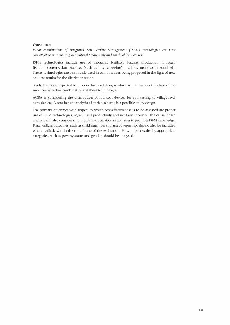
93
Question 4What combinations of Integrated Soil Fertility Management (ISFM) technologies are most
cost-effective in increasing agricultural productivity and smallholder incomes?
ISFM technologies include use of inorganic fertilizer, legume production, nitrogen fixation, conservation practices (such as inter-cropping) and [one more to be supplied]. These technologies are commonly used in combination, being proposed in the light of new soil test results for the district or region.
Study teams are expected to propose factorial designs which will allow identification of the most cost-effective combinations of these technologies.
AGRA is considering the distribution of low-cost devices for soil testing to village-level agro-dealers. A cost-benefit analysis of such a scheme is a possible study design.
The primary outcomes with respect to which cost-effectiveness is to be assessed are proper use of ISFM technologies, agricultural productivity and net farm incomes. The causal chain analysis will also consider smallholder participation in activities to promote ISFM knowledge. Final welfare outcomes, such as child nutrition and asset ownership, should also be included where realistic within the time frame of the evaluation. How impact varies by appropriate categories, such as poverty status and gender, should be analysed.
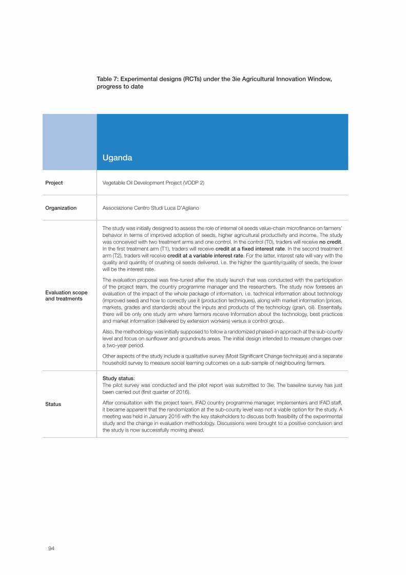
94
Table 7: Experimental designs (RCTs) under the 3ie Agricultural Innovation Window, progress to date
Uganda
Project Vegetable Oil Development Project (VODP 2)
Organization Associazione Centro Studi Luca D’Agliano
Evaluation scope and treatments
The study was initially designed to assess the role of internal oil seeds value-chain microfinance on farmers’ behavior in terms of improved adoption of seeds, higher agricultural productivity and income. The study was conceived with two treatment arms and one control. In the control (T0), traders will receive no credit. In the first treatment arm (T1), traders will receive credit at a fixed interest rate. In the second treatment arm (T2), traders will receive credit at a variable interest rate. For the latter, interest rate will vary with the quality and quantity of crushing oil seeds delivered, i.e. the higher the quantity/quality of seeds, the lower will be the interest rate.
The evaluation proposal was fine-tuned after the study launch that was conducted with the participation of the project team, the country programme manager and the researchers. The study now foresees an evaluation of the impact of the whole package of information, i.e. technical information about technology (improved seed) and how to correctly use it (production techniques), along with market information (prices, markets, grades and standards) about the inputs and products of the technology (grain, oil). Essentially, there will be only one study arm where farmers receive Information about the technology, best practices and market information (delivered by extension workers) versus a control group.
Also, the methodology was initially supposed to follow a randomized phased-in approach at the sub-county level and focus on sunflower and groundnuts areas. The initial design intended to measure changes over a two-year period.
Other aspects of the study include a qualitative survey (Most Significant Change technique) and a separate household survey to measure social learning outcomes on a sub-sample of neighbouring farmers.
Status
Study status: The pilot survey was conducted and the pilot report was submitted to 3ie. The baseline survey has just been carried out (first quarter of 2016).
After consultation with the project team, IFAD country programme manager, implementers and IFAD staff, it became apparent that the randomization at the sub-county level was not a viable option for the study. A meeting was held in January 2016 with the key stakeholders to discuss both feasibility of the experimental study and the change in evaluation methodology. Discussions were brought to a positive conclusion and the study is now successfully moving ahead.
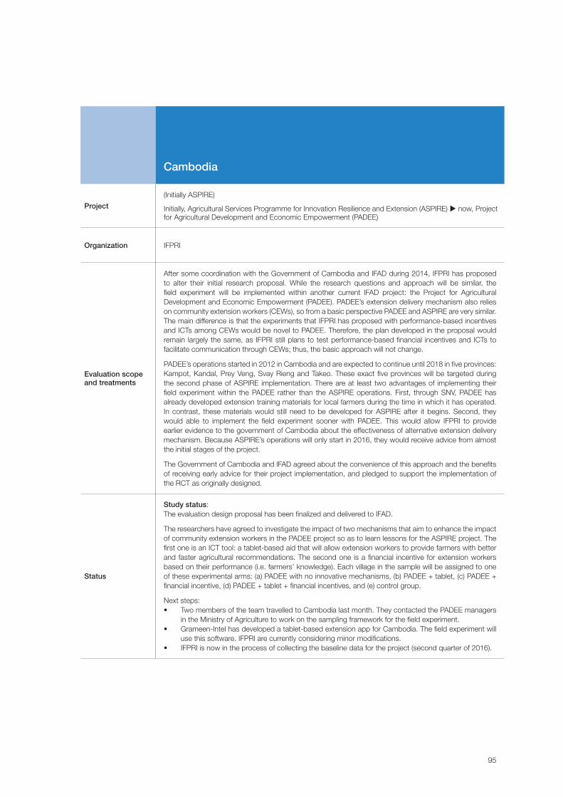
95
Cambodia
Project
(Initially ASPIRE)
Initially, Agricultural Services Programme for Innovation Resilience and Extension (ASPIRE) u now, Project for Agricultural Development and Economic Empowerment (PADEE)
Organization IFPRI
Evaluation scope and treatments
After some coordination with the Government of Cambodia and IFAD during 2014, IFPRI has proposed to alter their initial research proposal. While the research questions and approach will be similar, the field experiment will be implemented within another current IFAD project: the Project for Agricultural Development and Economic Empowerment (PADEE). PADEE’s extension delivery mechanism also relies on community extension workers (CEWs), so from a basic perspective PADEE and ASPIRE are very similar. The main difference is that the experiments that IFPRI has proposed with performance-based incentives and ICTs among CEWs would be novel to PADEE. Therefore, the plan developed in the proposal would remain largely the same, as IFPRI still plans to test performance-based financial incentives and ICTs to facilitate communication through CEWs; thus, the basic approach will not change.
PADEE’s operations started in 2012 in Cambodia and are expected to continue until 2018 in five provinces: Kampot, Kandal, Prey Veng, Svay Rieng and Takeo. These exact five provinces will be targeted during the second phase of ASPIRE implementation. There are at least two advantages of implementing their field experiment within the PADEE rather than the ASPIRE operations. First, through SNV, PADEE has already developed extension training materials for local farmers during the time in which it has operated. In contrast, these materials would still need to be developed for ASPIRE after it begins. Second, they would able to implement the field experiment sooner with PADEE. This would allow IFPRI to provide earlier evidence to the government of Cambodia about the effectiveness of alternative extension delivery mechanism. Because ASPIRE’s operations will only start in 2016, they would receive advice from almost the initial stages of the project.
The Government of Cambodia and IFAD agreed about the convenience of this approach and the benefits of receiving early advice for their project implementation, and pledged to support the implementation of the RCT as originally designed.
Status
Study status: The evaluation design proposal has been finalized and delivered to IFAD.
The researchers have agreed to investigate the impact of two mechanisms that aim to enhance the impact of community extension workers in the PADEE project so as to learn lessons for the ASPIRE project. The first one is an ICT tool: a tablet-based aid that will allow extension workers to provide farmers with better and faster agricultural recommendations. The second one is a financial incentive for extension workers based on their performance (i.e. farmers’ knowledge). Each village in the sample will be assigned to one of these experimental arms: (a) PADEE with no innovative mechanisms, (b) PADEE + tablet, (c) PADEE + financial incentive, (d) PADEE + tablet + financial incentives, and (e) control group.
Next steps: • Two members of the team travelled to Cambodia last month. They contacted the PADEE managers
in the Ministry of Agriculture to work on the sampling framework for the field experiment. • Grameen-Intel has developed a tablet-based extension app for Cambodia. The field experiment will
use this software. IFPRI are currently considering minor modifications.• IFPRI is now in the process of collecting the baseline data for the project (second quarter of 2016).
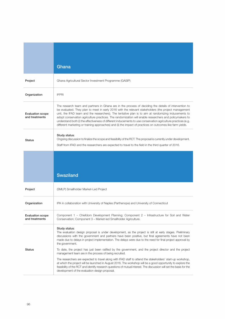
96
Ghana
Project Ghana Agricultural Sector Investment Programme (GASIP)
Organization IFPRI
Evaluation scope and treatments
The research team and partners in Ghana are in the process of deciding the details of intervention to be evaluated. They plan to meet in early 2016 with the relevant stakeholders (the project management unit, the IFAD team and the researchers). The tentative plan is to aim at randomizing inducements to adopt conservation agriculture practices. The randomization will enable researchers and policymakers to understand both (i) the effectiveness of different inducements to use conservation agriculture practices (e.g. different marketing or training approaches) and (ii) the impact of practices on outcomes like farm yields.
Status
Study status: Ongoing discussion to finalize the scope and feasibility of the RCT. The proposal is currently under development.
Staff from IFAD and the researchers are expected to travel to the field in the third quarter of 2016.
Swaziland
Project (SMLP) Smallholder Market-Led Project
Organization IPA in collaboration with University of Naples (Parthenope) and University of Connecticut
Evaluation scope and treatments
Component 1 – Chiefdom Development Planning; Component 2 – Infrastructure for Soil and Water Conservation; Component 3 – Market-led Smallholder Agriculture.
Status
Study status: The evaluation design proposal is under development, as the project is still at early stages. Preliminary discussions with the government and partners have been positive, but final agreements have not been made due to delays in project implementation. The delays were due to the need for final project approval by the government.
To date, the project has just been ratified by the government, and the project director and the project management team are in the process of being recruited.
The researchers are expected to travel along with IFAD staff to attend the stakeholders’ start-up workshop, at which the project will be launched in August 2016. The workshop will be a good opportunity to explore the feasibility of the RCT and identify research questions of mutual interest. The discussion will set the basis for the development of the evaluation design proposal.
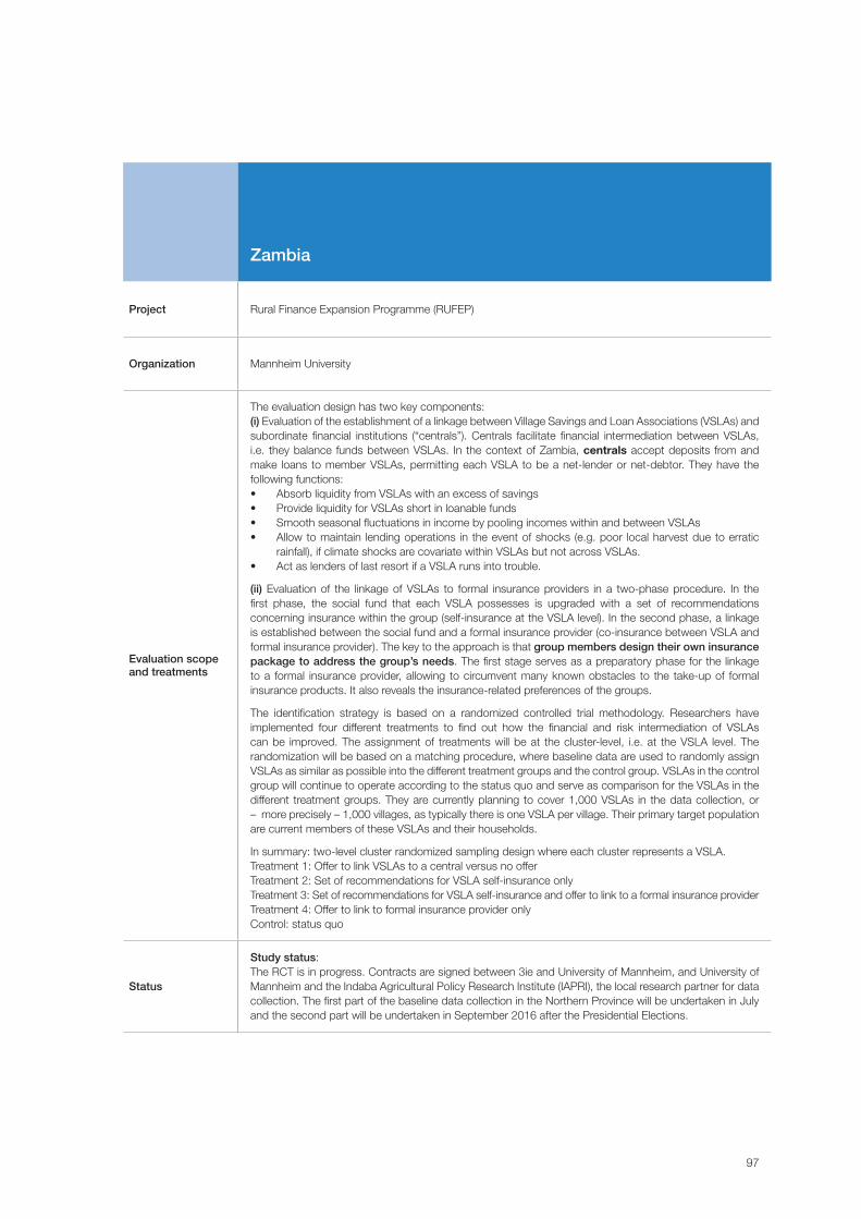
97
Zambia
Project Rural Finance Expansion Programme (RUFEP)
Organization Mannheim University
Evaluation scope and treatments
The evaluation design has two key components:(i) Evaluation of the establishment of a linkage between Village Savings and Loan Associations (VSLAs) and subordinate financial institutions (“centrals”). Centrals facilitate financial intermediation between VSLAs, i.e. they balance funds between VSLAs. In the context of Zambia, centrals accept deposits from and make loans to member VSLAs, permitting each VSLA to be a net-lender or net-debtor. They have the following functions:• Absorb liquidity from VSLAs with an excess of savings• Provide liquidity for VSLAs short in loanable funds• Smooth seasonal fluctuations in income by pooling incomes within and between VSLAs• Allow to maintain lending operations in the event of shocks (e.g. poor local harvest due to erratic
rainfall), if climate shocks are covariate within VSLAs but not across VSLAs. • Act as lenders of last resort if a VSLA runs into trouble.
(ii) Evaluation of the linkage of VSLAs to formal insurance providers in a two-phase procedure. In the first phase, the social fund that each VSLA possesses is upgraded with a set of recommendations concerning insurance within the group (self-insurance at the VSLA level). In the second phase, a linkage is established between the social fund and a formal insurance provider (co-insurance between VSLA and formal insurance provider). The key to the approach is that group members design their own insurance package to address the group’s needs. The first stage serves as a preparatory phase for the linkage to a formal insurance provider, allowing to circumvent many known obstacles to the take-up of formal insurance products. It also reveals the insurance-related preferences of the groups.
The identification strategy is based on a randomized controlled trial methodology. Researchers have implemented four different treatments to find out how the financial and risk intermediation of VSLAs can be improved. The assignment of treatments will be at the cluster-level, i.e. at the VSLA level. The randomization will be based on a matching procedure, where baseline data are used to randomly assign VSLAs as similar as possible into the different treatment groups and the control group. VSLAs in the control group will continue to operate according to the status quo and serve as comparison for the VSLAs in the different treatment groups. They are currently planning to cover 1,000 VSLAs in the data collection, or – more precisely – 1,000 villages, as typically there is one VSLA per village. Their primary target population are current members of these VSLAs and their households.
In summary: two-level cluster randomized sampling design where each cluster represents a VSLA. Treatment 1: Offer to link VSLAs to a central versus no offerTreatment 2: Set of recommendations for VSLA self-insurance onlyTreatment 3: Set of recommendations for VSLA self-insurance and offer to link to a formal insurance provider Treatment 4: Offer to link to formal insurance provider onlyControl: status quo
Status
Study status: The RCT is in progress. Contracts are signed between 3ie and University of Mannheim, and University of Mannheim and the Indaba Agricultural Policy Research Institute (IAPRI), the local research partner for data collection. The first part of the baseline data collection in the Northern Province will be undertaken in July and the second part will be undertaken in September 2016 after the Presidential Elections.
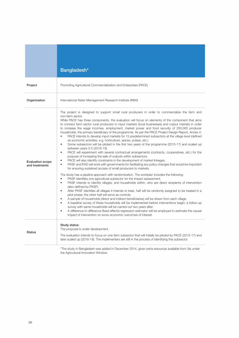
98
Bangladesh*
Project Promoting Agricultural Commercialization and Enterprises (PACE)
Organization International Water Management Research Institute (INWI)
Evaluation scope and treatments
The project is designed to support small rural producers in order to commercialize the farm and non-farm sector. While PACE has three components, the evaluation will focus on elements of the component that aims to connect farm sector rural producers to input markets (local businesses) and output markets in order to increase the wage incomes, employment, market power and food security of 250,000 producer households, the primary beneficiary of the programme. As per the PACE Project Design Report, Annex 4:• PACE intends to develop input markets for 15 predetermined subsectors at the village level (defined
as economic activities, e.g. horticulture, spices, pulses, etc.)• Some subsectors will be piloted in the first two years of the programme (2015-17) and scaled up
between years 3-5 (2018-19). • PACE will experiment with several contractual arrangements (contracts, cooperatives, etc.) for the
purpose of increasing the sale of outputs within subsectors.• PACE will also identify constraints in the development of market linkages.• PKSF and IFAD will work with governments for facilitating any policy changes that would be important
for ensuring sustained access of small producers to markets.
The study has a pipeline approach with randomization. The workplan includes the following:• PKSF identifies one agricultural subsector for the impact assessment. • PKSF intends to identify villages, and households within, who are direct recipients of intervention
(also defined by PKSF). • After PKSF identifies all villages it intends to treat, half will be randomly assigned to be treated in a
pilot phase; the other half will serve as controls. • A sample of households (direct and indirect beneficiaries) will be drawn from each village. • A baseline survey of these households will be implemented before interventions begin; a follow-up
survey with same households will be carried out two years after. • A difference-in-difference (fixed effects) regression estimator will be employed to estimate the causal
impact of intervention on socio-economic outcomes of interest.
Status
Study status: The proposal is under development.
The evaluation intends to focus on one farm subsector that will initially be piloted by PACE (2015-17) and later scaled up (2018-19). The implementers are still in the process of identifying this subsector.
*The study in Bangladesh was added in December 2014, given extra resources available from 3ie under the Agricultural Innovation Window.

99
Sensitivity analysis to different poverty lines
To check whether results would differ if an income-based poverty line were used, an analysis
of poverty dynamics was completed for four countries for which income data and a national
poverty line were available. Therefore, a sensitivity analysis to different poverty lines is
presented via kernel densities for four countries with income and expenditure data.
Note that endline daily income and total expenditure distributions are presented for treatment
and control samples respectively in Egypt, Ethiopia, Colombia and the Philippines.
Relative asset-based poverty lines were converted into their income-based equivalent
so as to make it possible to plot them against the US$1.25 a day and national poverty
lines respectively.
Figure 31 points to the fact that income dynamics exhibit wider gains for treatment relative to
the comparison sample beyond the 40th percentile cut-offs of the income distribution. This
highlights the fact that higher thresholds for the choice of the relative poverty lines would
be more appropriate, particularly if one considers the project-specific targeting. Results are
highly sensitive to the choice of the poverty lines. Overall, the expectation is that an income-
based poverty line would end up with a similar aggregate impact. However, the US$1.25
poverty line lies at the margin of the distribution, indicating that very few households (both
in the treatment and comparison groups) would be classified as poor.
Egypt:National poverty line: US$2.00 Purchasing Power Parity (PPP) per day in 2014 (income).
Set by Egypt’s Central Agency for Public Mobilization and Statistics (CAPMAS).
This poverty line amounts to 11 Egyptian pounds per day.
The income-expenditure equivalent poverty line at 40th percentile in Egypt was 25.60 Egyptian
pounds per day.
The income-expenditure equivalent poverty line at 60th percentile in Egypt was 32.21 Egyptian
pounds per day.
Ethiopia: National poverty line: US$1.24 PPP per day in 2015 (income).
Set by Ethiopia’s Ministry of Finance and Economic Development (MOFED).
This poverty line amounts to 10.35 Ethiopian birr per day.
The income-expenditure equivalent poverty line at 40th percentile in Ethiopia was 47.01
Ethiopian birr per day.
The income-expenditure equivalent poverty line at 60th percentile in Ethiopia was 74.53
Ethiopian birr per day.
Philippines:National poverty line: 28.86 PhP in the first semester of 2014 in LCU and 1.5832 in US$ PPP
per day in 2014 when converted to PPP dollars at the same rate as the income data (18.229).
Set by the Philippines Statistics Authority (NSCB).
The income-expenditure equivalent poverty line at 40th percentile in the analysis was PPP
US$5.8937 (107.85 LCU).
The income-expenditure equivalent poverty line at 60th percentile in the analysis was PPP
US$11.717 (214.41 LCU).
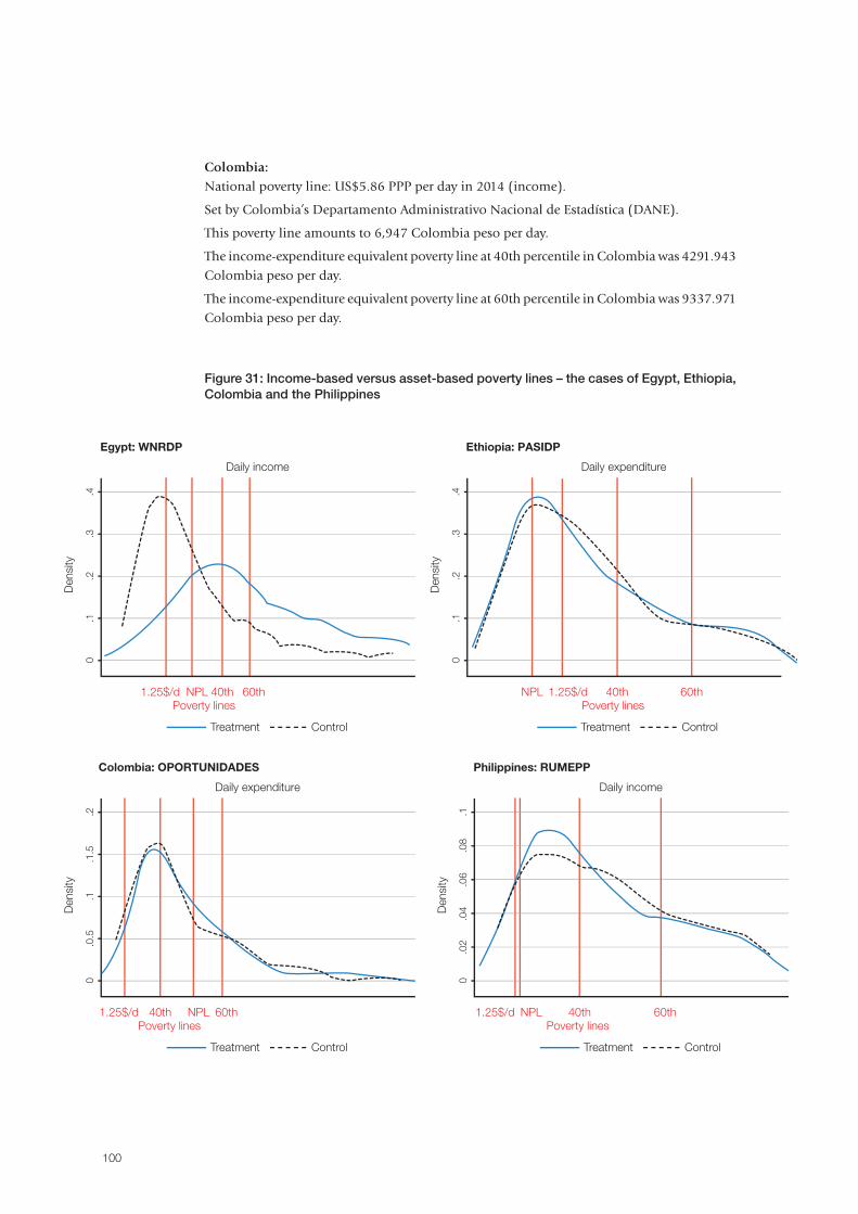
100
Colombia:National poverty line: US$5.86 PPP per day in 2014 (income).
Set by Colombia’s Departamento Administrativo Nacional de Estadística (DANE).
This poverty line amounts to 6,947 Colombia peso per day.
The income-expenditure equivalent poverty line at 40th percentile in Colombia was 4291.943 Colombia peso per day.
The income-expenditure equivalent poverty line at 60th percentile in Colombia was 9337.971 Colombia peso per day.
Figure 31: Income-based versus asset-based poverty lines – the cases of Egypt, Ethiopia, Colombia and the Philippines
101
Abadie, A., A. Diamond, and J. Hainmueller. 2010. Synthetic control methods for comparative case studies: Estimating the effect of California’s tobacco control program. Journal of the
American Statistical Association 105(490): 493-505.
Abadie, A., and G.W. Imbens. 2006. Large sample properties of matching estimators for average treatment effects. Econometrica 74(1): 235–267.
_____. 2008. On the failure of the bootstrap for matching estimators. Econometrica 76(6): 1537-1557.
_____. 2011. Bias-corrected matching estimators for average treatment effects. Journal of Business
and Economic Statistics 29(1): 1-11.
_____2012. Matching on the estimated propensity score. Harvard University and National Bureau of Economic Research. http://www.hks.harvard.edu/fs/aabadie/pscore.pdf.
Angrist, J.D., and J.S. Pischke. 2009. Mostly Harmless Econometrics: An Empiricist’s Companion.
Princeton: Princeton University Press.
Berelson, B. 1952. Content Analysis in Communication Research. Glencoe: Free Press.
Booysen, F., S. Van Der Berg, R. Burger, M. Von Maltitz, and G. Du Rand. 2008. Using an asset index to assess trends in poverty in seven Sub-Saharan African countries. World Development
36(6): 1113-1130.
Borenstein, M. H., L.V. Higgins, and J.P.T. Rothstein. 2009. Introduction to meta-analysis. Chichester: Wiley and Sons.
Brander, L.M., R.J. Florax, and J.E. Vermaat. 2006. The empirics of wetland valuation:
A comprehensive summary and a meta-analysis of the literature. Environmental and Resource
Economics 33(2): 223-250.
Busso, M., J. DiNardo, and J. McCrary. 2013. New evidence on the finite sample properties of propensity score reweighting and matching estimators. Working paper. University of California, Berkeley.
Cameron, A.C., and P.K. Trivedi. 2005. Microeconometrics: Methods and Applications. Cambridge: Cambridge University Press.
Caneiro, B., and A. Garbero. 2016. Supporting impact with evidence: A content analysis of Project Completion Reports. Working paper, International Fund for Agricultural Development, Rome.
Dang, H.A., P. Lanjouw, J. Luoto, and D. McKenzie. 2014. Using repeated cross-sections to explore movements into and out of poverty. Journal of Development Economics 107: 112-128.
Deeks, J.J. 2001. Systematic reviews in health care: Systematic reviews of evaluations of diagnostic and screening tests. British Medical Journal 323(7305): 157.
References
102
Dibba, L., A. Diagne, S.C. Fialor, and F. Nimoh. 2012. Diffusion and adoption of new rice
varieties for Africa (NERICA) in the Gambia. African Crop Science Journal 20(1).
Fields, G. S., and E.A. Ok. 1999. The Measurement of Income Mobility: An Introduction to the
Literature. New York: Springer.
Filmer, D., and L.H. Pritchett. 2001. Estimating wealth effects without expenditure data – or
tears: An application to educational enrollments in states of India. Demography 38(1): 115-132.
Filmer, D., and K. Scott. 2012. Assessing asset indices. Demography 49(1): 359-392.
Frankenberger, D., K. Swallo, M. Mueller, T. Spangler, J. Downen, and S. Alexander. 2013. Feed
the future learning agenda literature review: Improving resilience of vulnerable populations.
Technical report. Washington, D.C.: USAID.
Frölich, M. 2004. Finite-sample properties of propensity-score matching and weighting
estimators. Review of Economics and Statistics 86(1): 77–90.
Garbero, A. 2014a. Estimating poverty dynamics using synthetic panels for IFAD-supported
projects: A case study from Vietnam. Journal of Development Effectiveness 6(4): 490-510.
_____. 2014b. The IFAD9 Impact Evaluation Initiative: Sourcebook. Working paper.
Rome: IFAD.
Garbero, A., V. Brailovskaya, and B. Giera. 2016. Reconstructing the impact of IFAD-supported
projects on poverty reduction: Results from 14 IFAD-supported projects using observational
data. Working paper. Rome: IFAD.
Garbero, A., P. Marion, and V. Brailovskaya. 2016. Meta-analysis: The impact of agricultural
research on poverty. Working paper. Rome: IFAD.
Garbero, A., and G. Pacillo. 2013. Statistics and Studies for Development Division (SSD)
Inventory report. Working paper. Rome: IFAD.
Glass, G. V. 1976. Primary, secondary, and meta-analysis of research. Educational Researcher
5(10): 3-8.
Fizbein, A., N. Schady, F.H.G. Ferreira, M. Grosh, N. Kelleher, P. Olinto, and E. Skoufias. 2009.
Conditional cash transfers: Reducing present and future poverty. Technical report. Washington, D.C.:
World Bank.
Heckman, J. 1997. Instrumental variables: A study of implicit behavioral assumptions used in
making program evaluations. Journal of Human Resources 32 (3), 441-462.
Heckman, J.J., H. Ichimura, and P. Todd. 1997. Matching as an econometric evaluation
estimator: Evidence from evaluating a job training program. Review of Economic Studies 64(4):
605-654.
Heckman, J., and S. Navarro-Lozano. 2004. Using matching, instrumental variables, and
control functions to estimate economic choice models. Review of Economics and statistics 86(1):
30-57.
Hirano, K., and G.W. Imbens. 2001. Estimation of causal effects using propensity score
weighting: An application to data on right heart catheterization. Health Services and Outcomes
Research Methodology 2(3-4): 259-278.
Hirano, K., G. Imbens, and G. Ridder. 2003. Efficient estimation of average treatment effects
using the estimated propensity score. Econometrica 71(4): 1307–1338.
103
Holland, P.W. 1986. Statistics and causal inference. Journal of the American Statistical Association
81(396): 945-960.
Howe, L. D., B. Galobardes, A. Matijasevich, D. Gordon, D. Johnston, O. Onwujekwe, R. Patel,
E.A. Webb, D.A. Lawlor, and J.R. Hargreaves. 2012. Measuring socio-economic position for
epidemiological studies in low-and middle-income countries: A methods of measurement in
epidemiology paper. International Journal of Epidemiology 41(3): 871-886.
Howe, L. D., J.R. Hargreaves, S. Gabrysch, and S.R. Huttly. 2009. Is the wealth index a proxy for
consumption expenditure? A systematic review. Journal of Epidemiology and Community Health
63(11): 871-877.
Huber, M., M. Lechner, and C. Wunsch. 2010. How to control for many covariates? Reliable
estimators based on the propensity score. Working paper. Bonn: Institute for the Study of Labor.
International Fund for Agricultural Development (IFAD). 2010. Peer Review of IFAD’s Office of
Evaluation and Evaluation Function. EC 2010/62/W.P.2. Rome: IFAD.
_____. 2011. Action plan for strengthening the self-evaluation system. EB 2011/103/R.6.
Rome: IFAD.
_____. 2012a. Methodologies for Impact Assessments for IFAD9. EB 2012/107/INF.7.
Rome: IFAD.
_____. 2012b. Report of the Consultation on the Ninth Replenishment of IFAD’s Resources. GC
35/L.4. Rome: IFAD.
_____. 2015a. An update on the methodology for estimating the number of people moved
out of poverty and preparatory work for the impact assessment exercise during IFAD10. EB
2015/114/INF.3. Rome: IFAD.
_____. 2015b. Jharkhand-Chhattisgarh Tribal Development Programme: Impact Evaluation.
Rome: IFAD.
_____. 2016. Synthesis of lessons learned from the IFAD9 Impact Assessment Initiative. EB
2016/117/R.8/Rev.1. Rome: IFAD.
Imai, K., and Ratkovic, M. 2014. Covariate balancing propensity score. Journal of the Royal
Statistical Society: Series B (Statistical Methodology) 76(1): 243-263.
Imbens, G.W. 2004. Nonparametric estimation of average treatment effects under exogeneity:
A review. Review of Economics and Statistics 86(1): 4-29.
Imbens, G. W., W.K. Newey, and G. Ridder. 2005. Mean-square-error calculations for average
treatment effects. Working paper, University of California, Berkeley.
Imbens, G. W., and J.M. Wooldridge. 2009. New developments in econometrics. Lecture notes.
London: University College London.
Kolenikov, S., and G. Angeles. 2004. The use of discrete data in PCA: Theory, simulations, and
applications to socioeconomic indices. Chapel Hill: Carolina Population Center, University of
North Carolina.
Mendola, M. 2007. Agricultural technology adoption and poverty reduction: A propensity-score
matching analysis for rural Bangladesh. Food policy 32(3): 372-393.
Pradhan, M., and M. Ravallion. 1998. Measuring poverty using qualitative perceptions of welfare.
Working paper. Washington, D.C.: World Bank.

Ravallion, M, 1992. Poverty comparisons: A guide to concepts and measures. Working paper. Washington, D.C.: World Bank.
Robins, J.M., and A. Rotnitzky. 1995. Semiparametric efficiency in multivariate regression models with missing data. Journal of the American Statistical Association 90(429): 122-129.
Robins, J. M., A. Rotnitzky, and L.P. Zhao. 1994. Estimation of regression coefficients when some regressors are not always observed. Journal of the American Statistical Association 89(427): 846-866.
Rosenbaum, P. R. 2002. Observational Studies. New York: Springer.
Rosenbaum, P. R., and D.B. Rubin. 1983. The central role of the propensity score in observational studies for causal effects. Biometrika 70(1): 41–55.
Rubin, D. B. 1974. Estimating causal effects of treatments in randomized and nonrandomized studies. Journal of Educational Psychology 66(5): 688.
_____. 2001. Using propensity scores to help design observational studies: Application to the tobacco litigation. Health Services and Outcomes Research Methodology 2(3-4), 169-188.
Sahn, D. E., and D.C. Stifel. 2000. Poverty comparisons over time and across countries in Africa. World Development 28(12): 2123-2155.
_____. 2003. Exploring alternative measures of welfare in the absence of expenditure data. Review of Income and Wealth 49(4): 463-489.
Shapiro, G., and J. Markoff. 1997. A matter of definition. In Text analysis for the social sciences:
Methods for drawing statistical inferences from texts and transcripts, eds. M.E. Palmquist, K.M. Carley, and T.A. Dale. Oxford: Routledge.
Shuai, C., Z. Li, and R. Sun. 2011. IFAD projects: Results and impact on poverty reduction in rural China. Outlook on AGRICULTURE 40(4): 329-336.
Silverman, D. 2011. Interpreting qualitative data. London: SAGE Publications.
Strauss, A.L. 1987. Qualitative analysis for social scientists. Cambridge: Cambridge University Press.
United Nations. 2015. Transforming our world: The 2030 Agenda for Sustainable Development. A/70/L.1. New York: United Nations.
Van Kerm, P. 2006. Comparisons of income mobility profiles (Vol. 36). Essex: Institute for Social and Economic Research.
Waddington, H., B. Snilstveit, J.G. Hombrados, M. Vojtkova, J. Anderson, and H. White.
2014. Farmer field schools for improving farming practices and farmer outcomes in low-and middle-income countries: A systematic review. Campbell Systematic Reviews 10(6).
Wall, M., and D. Johnston. 2008. Counting heads or counting televisions: Can asset-based measures of welfare assist policy-makers in Russia? Journal of Human Development 9(1): 131-147.
White, H. 2009. Theory-based impact evaluation: Principles and practice. Journal of Development
Effectiveness 1(3): 271-284.
Weber, R.P. 1990. Basic Content Analysis. London: SAGE Publications.
Wooldridge, J.M. 2007. Inverse probability weighted estimation for general missing data problems. Journal of Econometrics 141(2): 1281-1301.
Wooldridge, J.M. 2010. Econometric Analysis of Cross Section and Panel Data. Cambridge: MIT press.
104
The IFAD Research Series
01. Agricultural and rural development reconsidered
A guide to issues and debates
By Steve Wiggins
02. Migration and transformative pathways
A rural perspective
By David Suttie, Rosemary Vargas-Lundius
03. Fostering inclusive outcomes in sub-Saharan African agriculture
Improving agricultural productivity and expanding agribusiness opportunities
ByDavidSuttie,RuiBenfica
04. The effects of smallholder agricultural involvement on household food consumption and dietary diversity
Evidence from Malawi
ByRuiBenfica,TalipKilic
05. Rural-urban linkages and food systems in sub-Saharan Africa
The rural dimension
By Karim Hussein, David Suttie
06. Why food and nutrition security matters for inclusive structural and rural transformation
By Steven Were Omamo
07. Measuring IFAD’s impact
Background paper to the IFAD9 Impact Assessment Initiative
By Alessandra Garbero