Measuring Euro Area Monetary Policy∗

Carlo Altavilla1 Luca Brugnolini2 Refet S. Gürkaynak3 Roberto Motto4

Giuseppe Ragusa5

1European Central Bank

2Una�liated

3Bilkent University, CEPR, CESIfo, & CFS

4European Central Bank

5University of Pisa

Abstract

We study the information �ow from the ECB on policy dates since its inception, using tick

data. We show that three factors capture about all of the variation in the yield curve but

that these are di�erent factors with di�erent variance shares in the window that contains

the policy decision announcement and the window that contains the press conference. We

also show that the QE-related policy factor has been dominant in the recent period and

that Forward Guidance and QE e�ects have been very persistent on the longer-end of the

yield curve. We further show that broad and banking stock indices' responses to monetary

policy surprises depended on the perceived nature of the surprises. We �nd no evidence of

asymmetric responses of �nancial markets to positive and negative surprises, in contrast

to the literature on asymmetric real e�ects of monetary policy. Lastly, we show how

to implement our methodology for any policy-related news release, such as policymaker

speeches. To carry out the analysis, we construct the Euro Area Monetary Policy Event-

Study Database (EA-MPD). This database, which contains intraday asset price changes

around the policy decision announcement as well as around the press conference, is a

contribution on its own right and we expect it to be the standard in monetary policy

research for the euro area.

JEL Classi�cation: E43, E44, E52, E58, G12, G14.

Keywords: ECB policy surprise, event-study, intraday, persistence, asymmetry.

�May 19, 2019�

∗We thank Burcin K�sac�ko§lu, Sang Seok Lee, Kadir Özen, Giulio Nicoletti, Michael McMahon, and GiovanniRicco for comments. We also thank many colleagues for asking for this dataset and making us construct it.Gürkaynak's research was supported by funding from the European Research Council (ERC) under the Euro-pean Union's Horizon 2020 research and innovation program (grant agreement No. 726400). The databaseintroduced in this paper will be periodically updated.Corresponding authors: Carlo Altavilla: Monetary Analysis Division, ECB, 60314 Frankfurt am Main,Germany. carlo.altavilla@ecb.europa.eu; Luca Brugnolini: London, UK. lucabrugnolini@gmail.com; RefetGürkaynak: Bilkent University, Department of Economics, Bilkent University, 06800 Ankara, Turkey.refet@bilkent.edu.tr; Roberto Motto: Monetary Policy Strategy Division, ECB, 60314 Frankfurt am Main,Germany. roberto.motto@ecb.europa.eu; Giuseppe Ragusa: Department of Economics and Management,University of Pisa, 56124 Pisa, Italy. giuseppe.ragusa@unipi.it.The views expressed in this paper are those of the authors and do not necessarily re�ect those of the EuropeanCentral Bank or the Eurosystem.

1 Introduction

Monetary policy, for better or worse, has been on the forefront of cyclical policymaking in the

past two decades, especially during the Great Recession and the sovereign debt crisis. While

there is an extensive literature on the US monetary policy, a comprehensive understanding of

the ECB policy and its �nancial market e�ects are yet to materialize. This is partly due to

the lack of a systematic database of high frequency, intraday data for a broad class of asset

prices in the euro area of the kind that has been employed in the US for more than a decade.

This paper helps remedy both de�ciencies by constructing a long (by euro area standards)

time series of policy-date event studies for the euro area, which will be kept up to date, and

by using this data to measure and assess the ECB monetary policy. While our substantive

analysis focuses on the �nancial market e�ects of monetary policy in the euro area, the dataset

we construct to carry out the analysis is of independent interest. Our euro area monetary

policy event-study database (EA-MPD) features price changes for a broad class of assets and

various maturities, including Overnight Index Swaps (OIS), sovereign yields, stock prices, and

exchange rates. We have exercised considerable care in studying each event window to clean

outliers and misquotes, of which there were plenty early in the sample, to make sure that what

we report accurately re�ects the market reaction. We provide a description of the data, and

timing of events on ECB policy dates in section 2 and o�er details and event-by-event analysis

in an accompanying online appendix.

Monetary policy surprises in the euro area are not only multi-dimensional�we show the

existence of perceived policy Target, Timing, Forward Guidance, and Quantitative Easing (QE)

surprises�they are also revealed in a multi-step structure. A press release provides information

on the policy decision with no rationale and discussion, later followed by a press conference.

The information markets extract from these two events are distinct, and intraday data allows

us to measure these di�erent types of information separately. Our event-study database utilizes

the intraday data to form event windows bracketing about 10 minutes before the release of

monetary policy information, to about 10 minutes after. Employing tick data allows us to

separately compute asset price changes around the release of the monetary policy decision

at 13.45, and the reading of the statement and the following Q&A in the press conference

beginning at 14.30. The separate releases of the policy decision and the narrative information

di�erentiates euro area monetary policy information revelation from that of the US, where the

two happen simultaneously.

After brie�y presenting the event-study database, we use it to study monetary policy

1

surprises in the euro area and their e�ects on various �nancial market segments. To do so, we

employ the methods developed by Gürkaynak et al. (2005) and Swanson (2017) for the US and

use them in the two intraday windows of the euro area policy communication. The di�erence

in the nature of information released in these two windows provides a new understanding of

market participants' interpretation of monetary policy communication.

Our results show that, naturally, the preponderance of surprises in the press release window

are about the current setting of the policy rates, �Target� surprises, with no other statistically

signi�cant policy surprise factors. In the press conference window, as expected, there are no

Target surprises and the Path and QE surprises dominate. Interestingly, while our analysis

suggests that a Target factor does not even appear as a statistically signi�cant factor in the

press conference window, a di�erent factor, �Timing� emerges. This type of surprise captures

the revision of policy expectations by shifting the expected policy action between the current

meeting and the next or the one following, in a way that leaves longer-term policy expectations

about unchanged. In essence, market participants extract two distinct types of guidance from

the press conference. One that is informative about the medium run, peaking at about two

years�Forward Guidance�and one for the near future, peaking at about six months maturity�

what we call Timing.

The methodology we employ to extract QE surprises yields continuous measures of the

market surprise. Hence, in studying the asset price responses to QE, we are able to condition

on the size of the surprises rather than only on a binary variable that shows when a QE

announcement took place. This allows for a substantially more precise understanding of QE

e�ects and helps distinguish QE from Forward Guidance surprises, which were also frequent

during the Zero Lower Bound (ZLB) period.1 We �nd that both QE (after 2014) and Forward

Guidance surprises are active in the press conference window and that while Forward Guidance

a�ected the middle of the yield curve most heavily, with a peak e�ect at about two years, QE

e�ects get larger as maturity increases, peaking at the 10-year maturity. Surprises about

the current setting of monetary policy, which were present in the pre-ZLB period, never had

noticeable e�ects on the long-end of the yield curve. Having the quanti�ed QE surprises also

allows us to study the persistence of their e�ects better. Unlike in the US, where QE e�ects

were short lived, with a half-life of three months as estimated by Wright (2012), we estimate a

half-life of about one year in the euro area. Thus, ECB QE not only had substantial immediate

e�ects on yields, it also had long lasting e�ects.

1Although the e�ective lower bound turned out to be below zero, we maintain the convention of calling thebound ZLB.

2

We also study the e�ects of ECB policy surprises on di�erent sovereign yields, exchange

rates, and stock prices. Some of these were studied previously in the literature using the

combined press release and press conference windows (such as Andrade and Ferroni, 2016)

and in the separate windows but not including the QE surprises in the analysis (such as

Brand et al., 2010 and Leombroni et al., 2017). This paper is the �rst to look at intraday

data to separately study the press release and press conference windows and extract both

conventional and unconventional monetary policy communication surprises from both. It is

also the �rst not to assume only Target surprises take place in the press release and broadly

de�ned �communication� surprises in the press conference windows but to ask statistically

how many factors are present in each and to estimate factors that can be attributed to speci�c

types of communication. Importantly, this paper is also the �rst in presenting a market-based

identi�cation of QE surprises in the euro area that shows QE has narrowed spreads, rather

than identifying QE surprises by assuming that these have narrowed spreads.

In the limited cases where both the event window coverage and the monetary policy surprise

de�nitions overlap with the existing literature, our �ndings are in line with what is already

known�such as e�ects of Target surprises that are signi�cant for the short end of the yield

curve�and instills con�dence for the new results we report on the di�erence between Timing

and Forward Guidance, on the e�ects of QE, on persistence of these e�ects, on information and

stock market reactions, on nonlinearity, and �nally on using our methodology for the analysis

of policy news that do not come out on Governing Council policy dates.

On stock prices, we �nd that the reaction of broad and banking indices can only be under-

stood when the genuine policy surprises (perceived deviations of interest rates from the policy

rule) are separated from information e�ects (perceived information signaled by the central

bank on the current and future state). When studied using this lens, monetary policy has

had signi�cant e�ects on stock prices but there was signi�cant time variance in the perceived

variances of genuine policy and information surprises. We further �nd that the policy surprise

e�ects on stocks were persistent as were the e�ects of these surprises on longer-term interest

rates, especially for Forward Guidance and QE surprises.

Our �ndings on nonlinearity are noteworthy. We study whether the market responses to

positive and negative surprises are di�erent. A nascent literature is suggesting that in the US,

monetary policy has asymmetric real e�ects (Tenreyro and Thwaites, 2016; Barnichon and

Matthes, 2017). We �nd that in the euro area �nancial market participants do not perceive

monetary policy e�ects to be asymmetric with respect to positive surprises and negative in

providing asset price responses.

3

Lastly, we use our estimated factors of monetary policy surprises and show how to use

them to decompose any policy-related news e�ects into these four factors. In two illustrative

examples we show that policymaker speeches and newswire reports can have substantial ef-

fects on yields and that in the recent past there have been cases where the �nancial market

participants have extracted information on QE-related policy from such news.

The paper is organized as follows. In section 2 below, we discuss the ECB policy commu-

nication and our event-study database. Then, in section 3 we construct our surprises in terms

of Target, Timing, Forward Guidance, and QE factors of monetary policy in the two policy

communication windows, and discuss their features and plausibility. Section 4 presents asset

price responses to the monetary policy surprises using a linear model. In section 5 we turn to

stock price reactions and information e�ects. Section 6 studies the dynamics of the identi�ed

surprises in a daily VAR framework. In Section 7 we relax the linearity assumption and allow

for asymmetries. Lastly, in section 8, we show how to adapt our methodology to speeches and

other monetary policy events and in section 9 we o�er concluding thoughts.

2 Euro Area Monetary Policy Event-Study Database

One of the contributions of this paper is to develop a Euro Area Monetary Policy Event-Study

Database (EA-MPD). This section is an introductory manual for the dataset, which will be

periodically updated and made available. The underlying tick data come from the Thomson

Reuters Tick History database, and we report our transformations of those data rather than

the underlying data. Here, we �rst describe the monetary policy communication process in

the euro area and then concentrate on the features of the dataset that we develop to measure

the monetary policy surprises, delegating more technical details on the dataset construction

to online appendices.

2.1 A Primer on euro area monetary policy communication

At its inception in 1999, the ECB Governing Council took policy decisions twice a month,

whereas a press conference took place only once a month�on the �rst meeting of the month.

After November 2001 only one meeting per month was a policy meeting, taking place on

the �rst Thursday of the month, regularly accompanied by the press conferences, with some

exceptions (Ehrmann and Fratzscher 2009 discuss this policy communication structure). As

of January 2015, the frequency of monetary policy meetings has moved to a six-week cycle.

Table 1 shows summary information on ECB communication on policy dates and its changes

4

over time. The online appendix shows this information in more detail, meeting-by-meeting.2

Part of our job in creating the EA-MPD was to compile this information in detail so that

the intraday windows have the right coverage. On the day of a policy meeting, di�erent from

the US FOMC press release (and very helpfully for researchers), the ECB policy decision is

announced in two separate steps. First, at 13.45 Central European Time (CET) a brief press

release provides the policy decision without any explanation and rationale. Then, at 14.30 CET

the ECB President reads a prepared text, the Introductory Statement (IS), on the rationale

behind the decision, which market participants often perceive to be also informative about the

future path of monetary policy. It takes about 15 minutes for the President to read out the

statement and there is a follow up question-and-answer session with journalists that lasts for

about 45 minutes. Up to December 2014 the press release referred to the decision on policy

rates only, while announcements of non-standard measures were made in the Introductory

Statement during the press conference. Between January 2015 and January 2016 the press

release mentioned whether �further measures� (without stating what measures were decided)

will be announced during the press conference. As of March 2016, the content of the decisions

on non-standard policy measures has been included in the press release.

In constructing the database, we �rst cleanse the data of misquotes,3 then discretize the

data within each window by taking the last quote of each minute within the window, and then

use the median price in the 13:25-13:35 interval as the pre-press-release quote, and the median

price in the 14:00-14:15 as the post-press-release quote. Similarly, we take the median price in

the 14:15-14:25 interval as the pre-conference quote and the median price in the 15:40-15:50

interval as the post-conference quote.4 We make use of an interval rather than selecting a

particular minute to measure the pre- and post-event quotes in order to minimize the risk of

selecting a quote that is not representative. The changes reported in the database are changes

from the pre-event quote to the post-event quote for each communication window. We de�ne

2The Appendix is available online and is structured as follows: Appendix A provides details on the GoverningCouncil meeting frequencies, the information release structure on policy dates and other relevant informationsince the inception of the ECB. It also contains a table that shows the policy rate decision and any otherpolicy relevant announcements on each policy date. Appendix B describes our high-frequency dataset showingthe Reuters Identi�cation Code (RIC) and data availability, which varies by instrument under consideration.Appendix C explains the procedure we follow in cleaning the tick data. Appendix D describes the structure ofthe database and the main features of the instruments it covers. Appendix E shows the consistency checks wehave performed on the computed asset price/yield changes. Appendix F, describes the econometric procedureused in the paper to identify the market-based surprises. Lastly, Appendix G compares the market-basedsurprise time series we built with market commentary for the largest surprises of each type.

3Such misquotes, which did not re�ect actual market pricing, were prevalent especially early in the sample.4Note that while the post-press release and pre-conference quote intervals partially coincide (the minute

14:15 is common to both), this is not an issue for attributing asset price changes to the press release and tothe conference as both are non-event intervals. The post-press release quote window is 15 minutes rather than10 as trading has tended to be thin in this window on many policy dates.

5

the �monetary policy event� as the union of the press release and conference, and measure

changes in asset prices due to this event as the change from the pre-press release quote to the

post-conference quote. Figure 1 shows this timeline in stylized form.

The EA-MPD reports the asset price/yield changes we construct for the three event win-

dows in separate worksheets. In each worksheet a policy date is in the �rst column on each

row, and the following columns show changes in selected asset prices/yields. The assets cov-

ered are: OIS rates with 1, 3, 6 month, 1 to 10, 15, and 20 year maturities; German bund

yields with 3 and 6 month, 1 to 10, 15, 20, and 30 year maturities, French, Italian, and Spanish

sovereign yields with 2, 5, and 10 year maturities, the STOXX50E and the stock price index

comprising banks (SX7E), and the exchange rate of the euro. The EA-MPD is made available

as a supplement to this paper and will be regularly updated.

In our substantive analysis we start the sample in 2002 because from 1999 (the beginning of

the single currency in the Euro Area) to the end of 2001 our intraday OIS data are very noisy,

with large spikes and sparse quotes. To provide an illustration of the (cleansed) intraday

data, Figure 2 shows the changes in the 2-year Overnight Index Swap (OIS) rate around

the publication of the press release and around the press conference on four di�erent policy

meeting dates: 4 July 2013, 4 September 2014, 3 December 2015, and 7 September 2017. We

select the 2-year rate as it is of su�ciently long maturity to display movements in response to

announcements of non-standard as well as standard measures.

These four panels are illustrative of the di�erent cases in which the monetary policy sur-

prises may arise within the policy meeting day. Panel (a) displays no reaction of the 2-year OIS

rate in the press release window and a reaction in the conference window. This episode corre-

sponds to the ECB announcement in the press conference, �rst time ever, of formal Forward

Guidance on the future path of its policy rates, by stating that policy rates are expected to

remain at present or lower levels for an extended period of time. Panel (b) shows a reaction in

the press release window, with no further news a�ecting the OIS rate in the conference window.

This episode corresponds to the announcement of a cut in the ECB deposit rate announced

in the press release. Panel (c) depicts a policy date in which there are sizable movements

in both windows. This episode captures the �nancial markets' disappointment following the

ECB decision to increase the size of its QE program: markets evidently were expecting a larger

increase of QE, as well as a cut in the policy rate, as suggested also by survey expectations

among �nancial analysts gathered ahead of the policy meeting. Lastly, panel (d) shows a day

in which there is no surprise, either in the press release or the conference windows. Policy dates

like these are surprisingly rare; there is usually some news for the �nancial markets, especially

6

in the press conference window. While this discussion of the policy surprises on the basis

of intraday changes in the 2-year OIS rate is suggestive of a Target/Path/QE decomposition,

formally carrying out this analysis requires the simultaneous study of interest rates at di�erent

maturities, which are covered by our event-study database and analyzed in section 3 below.

Before turning to the measurement of surprises it is useful to brie�y note some of the

internal consistency and robustness checks we have carried out on the data. The Appendix

contains details and further checks. The raw changes and surprises we measure, and the

results of the analysis we do using these are mostly insensitive to changes in the measurement

windows. Our estimates would have been more or less the same if we had taken the last

quote instead of the median within the window or used wider or narrower windows. We have

also veri�ed that the changes and surprises are independent across the two windows, showing

that we are indeed measuring reactions to unanticipated news in the two windows and not

momentum e�ects that carry over from one window to the other.

Another important issue has to do with the US data release calendar, which makes the

initial unemployment claims release often overlap with the event windows in the Euro Area.

In the window that contains both an ECB policy communication and the US initial claims

release,5 although the two will be uncorrelated, if the short-term euro OIS rates respond to the

initial claims surprise the monetary policy surprise measures will be subject to measurement

error. We studied the impact of US initial claims surprises on short-term euro OIS rates and

found that even in the very rare cases where there are statistically signi�cant coe�cients, the

R2 coe�cients are in single digits, implying that the simultaneous release of US initial claims

does not introduce noticeable measurement error into the Euro Area monetary policy surprises

that we measure. For completeness we include these as control variables in the statistical work

we present in section 4. It is reassuring that whether we include this control or not has no

bearing on the results we report.

3 Measuring Policy Surprises in the Euro Area

Understanding the e�ects of monetary policy requires identifying orthogonal changes in the

policy stance. These changes may be orthogonal to the state of the economy, as in VAR

analysis�in which case they are usually called policy shocks�or they may be orthogonal to the

5In the window that does not overlap with the initial claims release there is no correlation between the USsurprise and the changes and surprises we measure for the Euro Area, again verifying that we are measuringproper surprises arising from monetary policy communication.

7

information set of �nancial market participants�in which case they are called (market-based)

policy surprises.

Using monetary policy surprises measured in daily or higher frequency one can study asset

price responses to monetary policy in a meaningful way. The very reasonable identifying

assumption here is that monetary policy does not respond to asset price changes within the

day, hence causality goes from monetary policy to asset prices and �nancial markets' reaction

to monetary policy can be studied. Work on related questions for the euro area have been done

by Brand et al. (2010), Jardet and Monks (2014), Andrade and Ferroni (2016), Leombroni et al.

(2017), Cieslak and Schrimpf (2018), Kane et al. (2018), Rogers et al. (2014), and Jaroci«ski

and Karadi (2018) among others. These papers collectively study the �nancial and real e�ects

of ECB policy measured using high frequency surprises, but do not do the decompositions of

surprises as we do.

All of these papers had to construct their own event-study database to carry out similar

analyses. The EA-MPD we provide, by virtue of being regularly updated, will eliminate this

sizable �xed cost of doing research on Euro Area monetary policy. In terms of the exercises we

carry out, our value added will be in estimating rather than assuming the number of di�erent

types of policy surprises market participants perceive and in naming these. The results of this

exercise are interesting and di�erent from what has been assumed so far. Our further value

added will be in covering the crisis period and measuring the e�ects of ECB non-standard

monetary policy measures over a range of �nancial assets and comparing their transmission

with that of standard policy measures, as well as measuring the persistence of responses and

possible asymmetry of these responses to positive and negative surprises. In particular, we

will be estimating the persistence of QE e�ects in the euro area using a precise, continuous

measure of QE surprises for the �rst time.

3.1 Identifying the surprises

We �rst measure monetary policy as a potentially two dimensional process with possible Tar-

get/Timing and Path (Forward Guidance) components, and then allow for a third dimension

after the onset of the �nancial crisis so as to capture the information about non-standard

measures and especially QE. As noted above, the ECB policy communication extends over

two separate windows where the policy action is �rst announced in a press release with no

motivation, and then a statement is read by the President, followed by a question-and-answer

session. Market participants may update their beliefs about the current stance and future

path of monetary policy in response to the press release as well as the press conference; hence

8

on each policy date, using intraday data, we measure two sets of surprises.

We construct the Target and Forward Guidance surprises following the methodology em-

ployed in Gürkaynak et al. (2005) and Gürkaynak (2005), who in turn build on the work of

Kuttner (2001), using Federal Funds futures quotes to measure policy surprises in the US.

The methodology of constructing the QE factor follows that of Swanson (2017). In particular,

we extract factors from changes in yields of risk-free rates at di�erent maturities, spanning

one-month to ten-years, in each of the two windows (press release and conference). Ideally,

the risk-free rate curve in the euro area would be proxied by the term structure of the OIS.

Unfortunately, however, at maturities longer than 2 years high-frequency data on the OIS

rates is only available after August 2011. Therefore, prior to that date we use yields on the

German sovereign yields as proxy for the risk-free rates. Using the German yields throughout

the period makes no signi�cant di�erence.

To extract monetary policy surprises that admit economic interpretation from these asset

price changes we estimate latent factors from changes in yields and rotate these factors. The

matrix Xj, j = {press release, press conference}, has changes in 1, 3, and 6-month and 1, 2,

5, and 10-year yields in its seven columns, with each row corresponding to a policy date. This

matrix is taken directly from the EA-MPD. The factor structure is

Xj = F jΛj + εj, (1)

where F are the common latent factors, Λ are the factor loadings, and ε are the idiosyncratic

variation of yields at di�erent maturities. We analyze the press release and press conference

windows separately and estimate the factors�common drivers of yield changes�by principal

components.

We test the number of statistically signi�cant factors in the two windows over the full

sample and the pre-QE samples. As shown in Table 2, we consistently �nd a single signi�cant

factor in the press release window in both periods, but �nd two factors in the press conference

window before QE and three in the full sample, suggesting the presence of a new factor in this

window in the QE period.6

The latent factors F j do not have clean interpretations as monetary policy surprises, so

6The full sample press conference window having three factors might also have been due to the two sub-samples having two factors each, but one of these being di�erent across the pre-QE and QE periods. But the�rst two factors of the pre-QE and full samples are exactly the same, ruling out this interpretation. Further,although utilizing the test for only the QE sample is undesirable due to the very low degrees of freedom onewould have, doing that nonetheless �nds three factors in the press conference window in the QE period.

9

we rotate the factors to make them interpretable. This method has been used frequently

since Gürkaynak et al. (2005) and was �rst applied to Euro Area data by Brand et al. (2010)

using intraday data. For our purposes, including the analysis of QE, the orthogonal factors

are identi�ed by imposing the following restrictions on the rotation matrix: (1) the second

and third (when the third factor is present) factors do not load on the one-month OIS; (2)

the rotation is such that the third factor has the smallest variance in the pre-crisis period

(2 January 2002 - 7 Aug 2008). Essentially, we are forcing two factors not to be correlated

with the one-month OIS (the standard measure of the immediate policy setting surprise) and

allowing for one of them to a�ect the yield curve such that this factor was not important in the

pre-crisis period.7 This factor will turn out to contribute only to the movements in the long-

end of the yield curve, and only be active post-2014, naturally leading to the QE factor label.

Extraction of this last factor is an application of the Swanson (2017) methodology to euro area

monetary policy data. It is important to recognize that what matters for these surprises is how

market participants interpret the policy news and how their expectations change following the

policy news; our �ndings are not about the type of signal the central bank aims to provide.

The sequential nature of these orthogonalizations is important to keep in mind to under-

stand the rotated factors. One factor is de�ned by orthogonality to the 1-month OIS change.

Another is de�ned by orthogonality to this, such that the two explain most of the variance

of the yields. The third factor is de�ned such that it is orthogonal to the �rst two and the

1-month OIS, and explains the minimal share of the pre-crisis variance.8

With these rotations, the �rst and only statistically signi�cant factor in the press release

window turns out to be the �Target� factor, which loads only on the short rates. As expected,

we �nd a Forward Guidance (Path) factor that is always present in the press conference

window. The existence of guidance by central banks predates the global �nancial crisis as

well as the explicit designation of �Forward Guidance� and even the adoption of statements

accompanying policy decisions. The Forward Guidance factor captures the revision in market

expectations about the future path of policy rates that are orthogonal to the current policy

surprise.

7Note that this would be a somewhat imperfect measure prior to November 2001, as over that periodthe Governing Council took policy decisions at a fortnightly frequency. (Note also that, as discussed above,although we make the event study entries for all dates available in the dataset, the analysis in this section andbeyond uses data beginning in 2002.) In that case, the one-month OIS covers the next meeting as well, hencemay capture changes in expectations about the next meeting in addition to the immediate policy surprise.There are very few, if any, quotes for the one-week OIS on many event dates. Otherwise utilizing that measurewould have solved the problem of frequency of meetings being higher than maturity of contract used for theperiod prior to November 2001.

8A more elaborate and formal presentation of the factor rotations is presented in the Appendix.

10

The other factor that is always present in the press conference window does not have

factor loadings that lead to a Target interpretation. That factor does not load on the 1-

month OIS much. This is mechanically possible because the rotation forces one factor to be

orthogonal to 1-month OIS but does not force the other factor to closely follow it. The other

factor in the press conference window turns out to be a �Timing� factor that captures the

shifts in market expectations over the next few meetings that leaves longer-term interest rates

essentially unchanged. It is therefore important to note that estimating a Target factor in

the press release window and a Timing factor in the press conference window are �ndings,

not assumptions. Similarly, the QE factor that loads only on longer-term yields is a �nding

interpretable this way, not ex-ante assumed.

The interpretable surprises we measure using the factor rotation are suitable for our research

questions. Other decompositions of surprises are also possible and the EA-MPD will facilitate

asking a variety of euro area monetary policy related questions. Some of the recent work

in this vein are Jaroci«ski and Karadi (2018), who use stock-bond correlations to identify

central bank information signaling as opposed to classical monetary policy surprises; Andrade

and Ferroni (2016), using index-linked swaps for the same purpose; and Cieslak and Schrimpf

(2018), who use stocks and interest rates of short and long maturities to do a three-way

decomposition between classical monetary policy surprises, information (on growth) surprises,

and risk premium surprises.

We have also experimented with alternative identifying assumptions. Since we found a

single factor in the press release window, identifying the Target factor by orthogonalizing with

respect to a second factor may have been misleading so we used the change in the one-month

OIS directly as the Target factor, which unsurprisingly made no di�erence. Similarly, not

using the one-month OIS in the conference window (where it has negligible variance) and

using orthogonality to three-month OIS to do the factor rotation gave qualitatively the same

results. Many other ways of identifying surprises are possible and will surely be used by other

researchers.

3.2 Policy surprises in the euro area

Figure 3 shows the loadings of the rotated factors over the seven maturities in the analysis.

As the factors are identi�ed up to scale, we scale them such that Target has unit e�ect on

one-month OIS, Timing has unit e�ect on six-month OIS, Forward Guidance has unit e�ect on

the two-year and QE has unit e�ect on the ten-year yields. This normalization has no e�ect

on the variance shares and statistical signi�cance of the results we report.

11

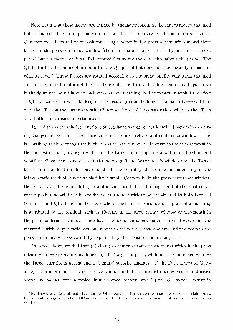
Note again that these factors are de�ned by the factor loadings, the shapes are not assumed

but estimated. The assumptions we made are the orthogonality conditions discussed above.

Our statistical tests tell us to look for a single factor in the press release window and three

factors in the press conference window (the third factor is only statistically present in the QE

period but the factor loadings of all rotated factors are the same throughout the period. The

QE factor has the same de�nition in the pre-QE period but does not show activity, consistent

with its label.) Those factors are rotated according to the orthogonality conditions assumed

so that they may be interpretable. In the event, they turn out to have factor loadings shown

in the �gure and admit labels that have economic meaning. Notice in particular that the e�ect

of QE was consistent with its design: the e�ect is greater the longer the maturity��recall that

only the e�ect on the current-month OIS are set (to zero) by construction, whereas the e�ects

on all other maturities are estimated.9

Table 3 shows the relative contribution (variance shares) of our identi�ed factors in explain-

ing changes across the risk-free rate curve in the press release and conference windows. This

is a striking table showing that in the press release window yield curve variance is greatest in

the shortest maturity to begin with, and the Target factor captures about all of the short-end

volatility. Since there is no other statistically signi�cant factor in this window and the Target

factor does not load on the long-end at all, the volatility of the long-end is entirely in the

idiosyncratic residual, but this volatility is small. Conversely, in the press conference window,

the overall volatility is much higher and is concentrated on the longer-end of the yield curve,

with a peak in volatility at two to �ve years, the maturities that are a�ected by both Forward

Guidance and QE. Thus, in the cases where much of the variance of a particular maturity

is attributed to the residual, such as 10-years in the press release window or one-month in

the press conference window, these have the lowest variances across the yield curve and the

maturities with largest variances, one-month in the press release and two and �ve-years in the

press conference windows are fully explained by the measured policy surprises.

As noted above, we �nd that (a) changes of interest rates at short maturities in the press

release window are mainly explained by the Target surprise, while in the conference window

the Target surprise is absent and a �Timing� surprise emerges; (b) the Path (Forward Guid-

ance) factor is present in the conference window and a�ects interest rates across all maturities

above one month, with a typical hump-shaped pattern, and (c) the QE factor, present in

9ECB used a variety of maturities for its QE program, with an average maturity of almost eight years.Hence, �nding largest e�ects of QE on the long-end of the yield curve is as reasonable in the euro area as inthe US.

12

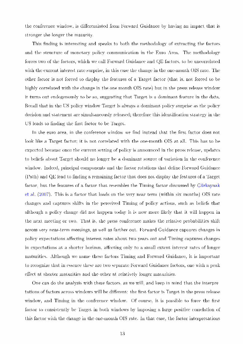
the conference window, is di�erentiated from Forward Guidance by having an impact that is

stronger the longer the maturity.

This �nding is interesting and speaks to both the methodology of extracting the factors

and the structure of monetary policy communication in the Euro Area. The methodology

forces two of the factors, which we call Forward Guidance and QE factors, to be uncorrelated

with the current interest rate surprise, in this case the change in the one-month OIS rate. The

other factor is not forced to display the features of a Target factor (that is, not forced to be

highly correlated with the change in the one month OIS rate) but in the press release window

it turns out endogenously to be so, suggesting that Target is a dominant feature in the data.

Recall that in the US policy window Target is always a dominant policy surprise as the policy

decision and statement are simultaneously released; therefore this identi�cation strategy in the

US leads to �nding the �rst factor to be Target.

In the euro area, in the conference window we �nd instead that the �rst factor does not

look like a Target factor; it is not correlated with the one-month OIS at all. This has to be

expected because once the current setting of policy is announced in the press release, updates

to beliefs about Target should no longer be a dominant source of variation in the conference

window. Indeed, principal components and the factor rotations that de�ne Forward Guidance

(Path) and QE lead to �nding a remaining factor that does not display the features of a Target

factor, but the features of a factor that resembles the Timing factor discussed by Gürkaynak

et al. (2007). This is a factor that loads on the very near term (within six months) OIS rate

changes and captures shifts in the perceived Timing of policy actions, such as beliefs that

although a policy change did not happen today it is now more likely that it will happen in

the next meeting or two. That is, the press conference makes the relative probabilities shift

across very near-term meetings, as well as farther out. Forward Guidance captures changes in

policy expectations a�ecting interest rates about two years out and Timing captures changes

in expectations at a shorter horizon, a�ecting only to a small extent interest rates of longer

maturities. Although we name these factors Timing and Forward Guidance, it is important

to recognize that in essence these are two separate Forward Guidance factors, one with a peak

e�ect at shorter maturities and the other at relatively longer maturities.

One can do the analysis with these factors, as we will, and keep in mind that the interpre-

tations of factors across windows will be di�erent: the �rst factor is Target in the press release

window, and Timing in the conference window. Of course, it is possible to force the �rst

factor to consistently be Target in both windows by imposing a large positive correlation of

this factor with the change in the one-month OIS rate. In that case, the factor interpretations

13

will be symmetric across windows, but this will come at the cost that less of the variance of

the conference window will be explained: Timing, which we have shown is important, would

have to turn into a residual. We continue with allowing for the Timing factor in the conference

window.

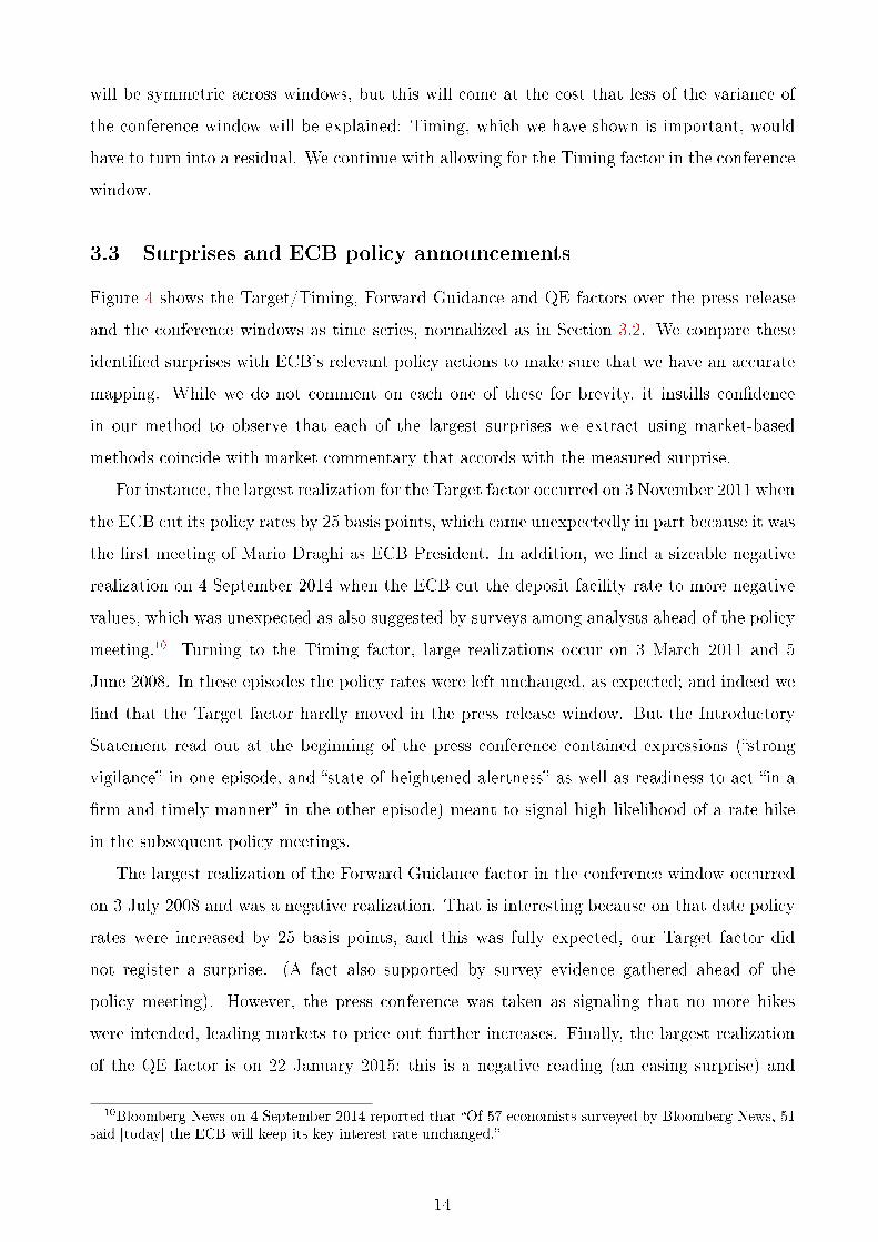
3.3 Surprises and ECB policy announcements

Figure 4 shows the Target/Timing, Forward Guidance and QE factors over the press release

and the conference windows as time series, normalized as in Section 3.2. We compare these

identi�ed surprises with ECB's relevant policy actions to make sure that we have an accurate

mapping. While we do not comment on each one of these for brevity, it instills con�dence

in our method to observe that each of the largest surprises we extract using market-based

methods coincide with market commentary that accords with the measured surprise.

For instance, the largest realization for the Target factor occurred on 3 November 2011 when

the ECB cut its policy rates by 25 basis points, which came unexpectedly in part because it was

the �rst meeting of Mario Draghi as ECB President. In addition, we �nd a sizeable negative

realization on 4 September 2014 when the ECB cut the deposit facility rate to more negative

values, which was unexpected as also suggested by surveys among analysts ahead of the policy

meeting.10 Turning to the Timing factor, large realizations occur on 3 March 2011 and 5

June 2008. In these episodes the policy rates were left unchanged, as expected; and indeed we

�nd that the Target factor hardly moved in the press release window. But the Introductory

Statement read out at the beginning of the press conference contained expressions (�strong

vigilance� in one episode, and �state of heightened alertness� as well as readiness to act �in a

�rm and timely manner� in the other episode) meant to signal high likelihood of a rate hike

in the subsequent policy meetings.

The largest realization of the Forward Guidance factor in the conference window occurred

on 3 July 2008 and was a negative realization. That is interesting because on that date policy

rates were increased by 25 basis points, and this was fully expected, our Target factor did

not register a surprise. (A fact also supported by survey evidence gathered ahead of the

policy meeting). However, the press conference was taken as signaling that no more hikes

were intended, leading markets to price out further increases. Finally, the largest realization

of the QE factor is on 22 January 2015; this is a negative reading (an easing surprise) and

10Bloomberg News on 4 September 2014 reported that �Of 57 economists surveyed by Bloomberg News, 51said [today] the ECB will keep its key interest rate unchanged.�

14

corresponds to the announcement of the ECB's asset purchase program, which was made in

the press conference.

A more detailed description of the time series of these surprises is relegated to the appendix.

While we present the surprises and the statements that led to these, a formal mapping between

quanti�ed words, as in Hansen and McMahon (2016) and the market perceptions we measure

here has to be a separate paper.

4 Asset Price Response to Policy

An important contribution of this paper is de�ning the interpretable policy surprise factors

for the euro area. Once the policy surprises are measured as described in Section 3, causality

is established, and the response of other asset prices can be studied via OLS. We estimate

the impact of monetary policy on sovereign yields, the exchange rate, and the stock market.

In the conference window we continue to use the surprise in the US initial jobless claims as

an additional control (labeled IJC) whenever we run regressions. Including or excluding the

initial claims makes essentially no di�erence to our coe�cients of interest.

4.1 Sovereign yields

Table 4 shows the intraday reaction of euro area risk-free rates to the Target surprise we

have identi�ed in the press release window (panel A) and the three surprises in the conference

window (panel B). This table presents the information in Figure 3 with numbers, the nor-

malized factor loadings using an OLS regression framework and controlling for the US Initial

Jobless Claims surprises in the press conference window. The loadings, which are essentially

unchanged compared to Figure 3 (the ECB policy surprises and US IJC surprises are not

correlated) show the estimated weights over maturities in the full sample.

An interesting question is whether these factors have behaved the same way throughout the

sample or whether the policy surprises elicited di�erent responses before the crisis, during it

before QE became a policy tool, and when QE was actively used. To study this, we run these

regressions with samples up to 2008, 2008-2014, and 2014 to september 2018, corresponding

to pre-crisis, crisis before QE, and QE periods. The QE factor is of course only active in the

last period.

Tables 5 to 7 show the results. Here, remember that these factors are de�ned as before

(loadings do not change across tables) and are normalized such that Target, Timing, Forward

Guidance, and QE factors have unit e�ects on one-month, six-month, two-year and 10-year

15

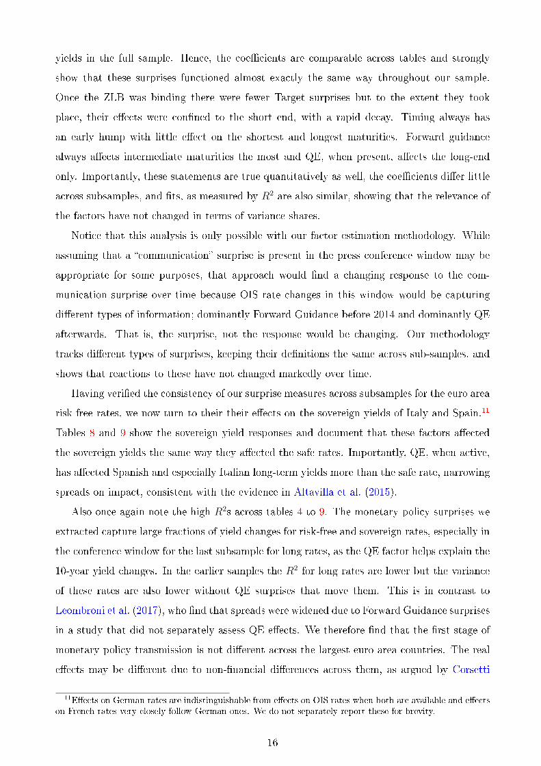
yields in the full sample. Hence, the coe�cients are comparable across tables and strongly

show that these surprises functioned almost exactly the same way throughout our sample.

Once the ZLB was binding there were fewer Target surprises but to the extent they took

place, their e�ects were con�ned to the short end, with a rapid decay. Timing always has

an early hump with little e�ect on the shortest and longest maturities. Forward guidance

always a�ects intermediate maturities the most and QE, when present, a�ects the long-end

only. Importantly, these statements are true quantitatively as well, the coe�cients di�er little

across subsamples, and �ts, as measured by R2 are also similar, showing that the relevance of

the factors have not changed in terms of variance shares.

Notice that this analysis is only possible with our factor estimation methodology. While

assuming that a �communication� surprise is present in the press conference window may be

appropriate for some purposes, that approach would �nd a changing response to the com-

munication surprise over time because OIS rate changes in this window would be capturing

di�erent types of information; dominantly Forward Guidance before 2014 and dominantly QE

afterwards. That is, the surprise, not the response would be changing. Our methodology

tracks di�erent types of surprises, keeping their de�nitions the same across sub-samples, and

shows that reactions to these have not changed markedly over time.

Having veri�ed the consistency of our surprise measures across subsamples for the euro area

risk-free rates, we now turn to their their e�ects on the sovereign yields of Italy and Spain.11

Tables 8 and 9 show the sovereign yield responses and document that these factors a�ected

the sovereign yields the same way they a�ected the safe rates. Importantly, QE, when active,

has a�ected Spanish and especially Italian long-term yields more than the safe rate, narrowing

spreads on impact, consistent with the evidence in Altavilla et al. (2015).

Also once again note the high R2s across tables 4 to 9. The monetary policy surprises we

extracted capture large fractions of yield changes for risk-free and sovereign rates, especially in

the conference window for the last subsample for long rates, as the QE factor helps explain the

10-year yield changes. In the earlier samples the R2 for long rates are lower but the variance

of these rates are also lower without QE surprises that move them. This is in contrast to

Leombroni et al. (2017), who �nd that spreads were widened due to Forward Guidance surprises

in a study that did not separately assess QE e�ects. We therefore �nd that the �rst stage of

monetary policy transmission is not di�erent across the largest euro area countries. The real

e�ects may be di�erent due to non-�nancial di�erences across them, as argued by Corsetti

11E�ects on German rates are indistinguishable from e�ects on OIS rates when both are available and e�ectson French rates very closely follow German ones. We do not separately report these for brevity.

16

et al. (2018) but that is a separate topic of study.

4.2 Exchange rate

Table 10 reports results for the euro-US dollar exchange rate, with the top panel focusing on

the press release window and the bottom panel on the conference window. In both windows

and along about all sub-samples, the surprises exert a statistically signi�cant e�ect on the

exchange value of the euro.

In the conference window all factors are highly signi�cant in the full sample and in most

of the sub-samples, with the response of the exchange rate becoming much stronger over

recent periods. For instance, a one unit change in the Forward Guidance factor leads to an

appreciation of 0.22 percent in last sub-sample, �ve times larger than in the previous one. The

R-squared of the regression is about 0.6, which is very large for work involving exchange rates

on the left-hand-side.

It is also noteworthy that in our samples the Rogers et al. (2014) �preserving the euro

e�ect� where easing surprises make the euro appreciate, does not manifest itself. This e�ect,

while certainly present on some days, is dominated by the standard uncovered interest parity

channel in the periods of our analysis.

These �ndings are broadly consistent with the work of Faust et al. (2007), who show that

�good news� in data releases in the US lead to an appreciation of the dollar and relate this

to uncovered interest parity. We �nd that higher rates than anticipated in the euro area

similarly lead to an appreciation of the euro, as expected. There is not much of a literature

on whether current rates or expected future interest rates, or short versus long-term interest

rates theoretically should be and empirically are the main drivers of exchange rates. Our

empirical �ndings suggest that changing interest rate expectations at all maturities as a result

of monetary policy communication a�ect the exchange value of the euro.

5 Stock Prices and the Information Surprise

Table 11 shows the intraday reaction of the euro area stock market to the Target surprise (panel

A) and the three surprises in the conference window (panel B). The response is statistically

signi�cant and negative (surprises that increase yields lead to stock index declines) for the

Target factor in the full sample and the pre-crisis sample, and for the Timing and Forward

Guidance factors in the post-2014 sample. Results for the stock market index comprising only

euro area banks are similar.

17

Lack of signi�cance for some of the factors in some sub-samples may be expected in light

of the recent literature arguing that any monetary policy decision (or no decision) may be

interpreted by markets in two di�erent ways: a textbook monetary policy shock or a perceived

revelation of information about the state of the economy. This latter type of policy is called

Delphic in Campbell et al. (2012) and information shock in Miranda-Agrippino and Ricco

(2018) and Jaroci«ski and Karadi (2018). For our analysis, it is important to note that the

responses of nominal rates to the two types of surprises are qualitatively similar. A positive

policy surprise increases yields if it is a genuine shock, but perceived information that the

state of the business cycle is stronger than thought also similarly increases yields by increasing

future expected short rates. Therefore, possible information e�ects do not interfere with our

identi�cation strategy of the factors.

However, the two types of surprises have opposite e�ects on stocks. Lower rates are good

news (lower discount rates and higher demand) but learning that the cyclical state is worse

than previously thought is bad news (lower dividends). One can see similar e�ects on in�ation

expectations; a positive policy surprise should decrease in�ation compensation implied by

indexed securities unless the surprise is perceived to be signalling information about high

in�ationary pressures, in which case in�ation compensation will increase. The macroeconomic

impacts of these policy surprises are also found to di�er depending on whether the policy

surprise triggers a positive or negative response of the stock market (Jaroci«ski and Karadi,

2018) or, similarly, a positive or negative response of in�ation-linked swaps (Andrade and

Ferroni, 2016), as measured at high-frequency around policy events.12 Therefore, the presence

of these two types of policy can make the response of the stock market, on average, insigni�cant

and can produce the results reported in Table 11.

To assess whether there is evidence of these two types of surprises in our dataset, for each

policy event we compare the sign of the response of the stock market and in�ation-linked

swaps. If nominal rates, stock prices and in�ation-linked swaps all move in the same direction,

this would suggest that information shocks may be prevailing. To overcome the problem that

data on in�ation compensation are not reliably available at intraday frequency, we adapt our

analysis to daily frequency and measure the interest rate reaction as the �tted value of the

one-day change (around the policy events) of the 2-year OIS regressed on the intraday factors.

We do the same for the one-day change of in�ation-linked swaps and the one-day log-di�erence

of stock prices.

12Jaroci«ski and Karadi (2018) use intraday data employing stocks whereas Andrade and Ferroni (2016) usedaily data due to lack of reliable intraday data for in�ation-linked swaps.

18

Figure 5 shows the dates for which stock prices and in�ation swaps move in the same

direction so that the market perception of policy can be clearly interpreted as information

(Delphic) surprises or pure policy (Odyssean) surprises.13 The �gure shows that there is a

marked di�erence across sub-samples in terms of the information market participants extract

from policy surprises. Whereas in the post-2014 sub-sample (bottom panel) information shocks

(de�ned as nominal interest rates, stock prices, and in�ation-linked swaps moving in the same

direction) are rare, these are frequent during the crisis sub-sample (top panel). That is, in the

crisis period market participants attributed more of the surprises they perceived to information

they thought the ECB has, consistent with a similar �nding for the US by Lunsford (2018).

To delve deeper into this issue we build a daily VAR. The identi�cation strategy is based

on the idea of using high-frequency monetary policy surprises to isolate the variation in the

reduced-form residuals in the VAR due to monetary policy shocks. The use of external instru-

ments for identi�cation in macroeconometric models goes back to Stock and Watson (2012)

and Mertens and Ravn (2013). We start the analysis by estimating the reduced form VAR as

described in equation (2).

Yt = c+

p∑j=1

BjYt−j + A0ut, (2)

where Yt is a vector consisting of the 2-year OIS, the log EUR-USD exchange rate, the log

of the stock market index (Euro Stoxx 50), and the 2-year in�ation linked swap (ILS2Y). As

we are only interested in the e�ects of monetary policy shocks, our objective is to identify the

column of the matrix A0 corresponding to the contemporaneous e�ect of the monetary policy

shock. The instrument must satisfy the relevance and exogeneity assumptions:

E(Ztumt ) = α 6= 0, E(Ztu

ot ) = 0, (3)

where Zt is the instrument, and umt and uot denote the monetary and the non-monetary shocks.

Our instruments will be the policy surprises we have identi�ed. The external instruments are

the Target factor (press release), the Timing, the Forward Guidance, and the QE factor (press

conference). As the VAR residual is a linear combination of structural shocks, we instrument

the residuals of the VAR with one instrument at a time, as we aim to extrapolate the component

correlated with the Target, Timing, Forward Guidance and Quantitative Easing surprises

13In about 80% of the policy dates stock prices and in�ation-linked swaps move in the same direction. Inthe other 20%, in almost all of the cases the stock price reaction is about zero and the in�ation-linked swapreaction is very small. Hence, these two measures almost never meaningfully disagree. Therefore, incidentally,our results verify Andrade and Ferroni (2016) and Jaroci«ski and Karadi (2018) methods against each otherand �nd that they are in agreement.

19

respectively. As a di�erent exercise, one can also include all the instruments simultaneously,

however, this will only help to identify a single monetary policy shock which re�ects a linear

combination of the four. To be consistent with the previous analysis, we use the intraday

factors as external instruments for the VAR estimated on all sub-samples. When analyzing

Quantitative Easing, the instrument is used on the period 2014-2018.

Figure 6 shows that in the post-2014 sub-sample each factor exerts a signi�cant impact,

with a decline in interest rates triggering a rise in stock prices and in�ation-linked swaps, and a

depreciation of the euro. In the 2008-2013 sub-sample the impact of each factor is signi�cant,

but we �nd that this time a decline in interest rates triggers a decline in stock prices and

in�ation linked-swaps, consistent with a perceived revelation of negative news. The exchange

rate is found to depreciate, suggesting that it does not react di�erently, at least qualitatively,

to an information shock. In the pre-crisis sub-sample of 2002-2007 we �nd that stock prices

go down in response to positive Target surprise while there is no clear pattern for Timing and

Forward Guidance surprises. Over that sub-sample we cannot use in�ation-linked swaps as

they become available only in 2005.

Overall, these results suggest that there is evidence of information shocks and that stock

prices and in�ation-linked swaps may both help in telling apart these shocks from the more

traditional policy shocks. We �nd that these results are fairly persistent, they do not only

manifest themselves on policy dates then disappear. The results also suggest that it is possible

to extend and generalise the macroeconomic analysis of Andrade and Ferroni (2016) and

Jaroci«ski and Karadi (2018). They use the overall policy surprise as measured by the high-

frequency change of the 2-year OIS around policy events. Our analysis shows that it is possible

to compute the macroeconomic response to each of the factors we have identi�ed including

QE. The important �nding of this section is that ECB policy surprises do have e�ects on stock

prices but to properly study these one needs to separate traditional surprises from perceived

information revelation, as we have brie�y shown here.

6 Persistence of Identi�ed Policy Surprises

An important and open question has to do with the longevity of �nancial market e�ects of

surprises identi�ed in high-frequency event studies. This has especially been important for the

debate over unconventional monetary policy, where immediate market reactions were visible

in real time in most occasions, but doubts lingered as to whether on balance these polices had

lasting e�ects. In particular, the e�ects of QE have been very di�cult to trace over time as

20

QE surprises were not quanti�ed and only the announcement times were known, leading to

the use of dummy variables to capture QE e�ects that were not very precisely estimated. An

important paper in this vein is Wright (2012) who traces the e�ects of Fed QE surprises in

a VAR identi�ed via heteroskedasticity. He �nds a half life of about three months, which is

economically signi�cant but not very long.

Our continuous measure of QE surprises allows estimating the persistence of QE e�ects

using much richer information than before. To gain insight about the persistence of the e�ects

of the ECB monetary policy measures, we use a small daily vector autoregression with �nancial

variables as in section 5, but we replace the 2-year OIS with the 10-year yield as we want to

focus on longer maturities, which our analysis in section 4 has shown to be a�ected the most by

QE. The measure of the 10-year yield we include in the model is the German, French, Italian

and Spanish 10-year sovereign yield, added one at the time. We keep in the vector Yt the other

variables we have used in the VAR in section 5: log of the EUR-USD exchange rate, the log

of the stock market index (Euro Stoxx 50), and the 2-year in�ation linked swap (ILS2Y). To

these measures, in the robustness check, we add the spread of the AAA and BBB corporate

yields, the EA implied stock volatility index � i.e., the VIX for the EA, and the 2-year OIS

and the 5-year EA GDP-weighted yields.14

Our data set is daily and covers the period 2005-03-31 to 2018-09-13, which is the longest

available for the selected variables. Consistent with the previous analysis, we use the Target,

Timing, and Forward Guidance factors as external instruments for the VAR estimated on the

full sample (2005-03-31 to 2018-09-13). In the Quantitative Easing cases, the instrument is

used on the period 2014-01-01 to 2018-09-13 only.

Figure 7 shows the results for Target (�rst column), Timing (second column), Forward

Guidance (third column) and Quantitative Easing (forth column) surprises on German, Italian,

French and Spanish 10-year government yields. The responses of all countries' yields are

strongly persistent. However, the chart also shows some heterogeneity. German and French

yields show a similar response to all shocks and similarly Italian and Spanish yield responses

are alike each other, but the two sets are di�erent. This is to be expected from the results on

spreads we have discussed earlier.

The results further show that for Target, the IRFs are not statistically di�erent from zero

after a few periods. This is not surprising in light of the results we have shown in section 4

documenting that Target does not have a material e�ect on 10-year yields on impact. Timing

14The GDP weighted 5-year EA yield is used instead of the 5-year OIS, as the latter is only available for ashort sample.

21

and Forward Guidance are more heterogeneous, even if in almost all the cases (except for Italy

for Timing) the response seems quite persistent. Finally, the QE shock is persistent and well

identi�ed as judged by the narrow con�dence bands. Our �nding of a half-life of about one

year for the QE e�ects is much longer than that of Wright (2012) for the US�at about three

months�which was obtained using QE announcement dates in a heteroskedasticity-based

estimation setting. It is also much longer than Swanson (2017), who estimates a persistence

in the US similar to Wright, using local projections. Andrade et al. (2016), using a shorter

sample, also �nd persistemt e�ects of QE in the euro area.

To further investigate these results, we check whether these �ndings are robust to di�erent

VAR speci�cations. Figure 8 shows the IRFs from a �Combinatoric� VAR (CVAR). The CVAR

works as follows: we add to the four variables we used in the previous speci�cation (10-year

sovereign yield, the log of the EUR-USD exchange rate, the log of the stock market index,

Euro Stoxx 50, and the 2-year in�ation linked swap, ILS2Y), four more variables (the BBB-

AAA corporate bond spread, the EA stock market implied volatility index (VSTOXX), the

2-year OIS and the 5-year EA GDP-weighted yields, and we specify a di�erent VAR for each

possible combination of two to eight variables. The 10-year yield is always included, as the

instrumented variable. Additionally, we ran each of these using eight di�erent speci�cations

of the 10-year yield,15 for a total of 8(27 − 1) ≈ 1000 speci�cations. For each model, we

always use the longest sample available. The �gure highlights that IRF coe�cients, estimated

from di�erent models, display a clear and persistent pattern. Especially the QE and Forward

Guidance surprises a�ected the 10-year yields for a long period of time.

It is interesting to �nd the persistence of unconventional policy in the euro area on long-

term interest rates to be much higher than what is found for the US. In interpreting this result

it is important to keep in mind the di�erence in methodologies. We employ a VAR with a

continuous measure for Forward Guidance and QE surprises as instruments for the euro area,

in contrast to heteroskedasticity-identi�ed VARs and local projections for the US. We note the

high and robust persistence of unconventional policy e�ects we �nd with the VAR but caution

that these results are not directly comparable to those in the literature for the US.

15As 10-year yields we include the German, Italian, Spanish and French yields, the OIS yields, the EAGDP-weighted yield, and the EA yields derived by the ECB using the Svensson (1994) methodology, utilizingAAA-rated euro area central government bonds and all euro area central government bonds (including AAA-rated).

22

7 Non-linearity

Starting with the seminal work of McCallum (1991), the monetary policy literature has paid

attention to possible asymmetric e�ects of monetary policy on real variables. In particular it

has studied the di�erent e�ects during expansions and recessions, good and bad credit market

conditions, and high or low in�ation regimes, with a general consensus that there is indeed

heterogeneity.16 The more recent literature, using Romer and Romer (2004) identi�cation and

Jordà (2005) local projections, �nds that monetary policy tightening has stronger e�ects than

loosening (Tenreyro and Thwaites, 2016; Barnichon and Matthes, 2017).

In this section we ask a related but distinct question and study whether market participants

perceive monetary policy e�ects di�erently when the surprise is positive versus negative. The

�nancial market reaction to monetary policy surprises captures the updates to beliefs of market

participants, which may not be the same as the actual future impact of monetary policy if there

are information asymmetries. Independently of whether market participants form �correct�

beliefs of monetary policy asymmetry, changes in asset prices are the �rst step of monetary

policy transmission and understanding whether there are asymmetries in the �nancial market

response to monetary policy is important in its own right. For brevity we do not repeat all of

our analysis allowing for asymmetries but present the salient cases that show the presence or

lack of asymmetric responses. We do this for risk free rates and sovereign yields by including

an indicator variable for negative surprises and allowing interactions.

Tables 12 to 14 report the results. These results are striking in their lack of asymmetry.

Across the three tables for the e�ects of policy surprises on euro area risk free rates and Italian

and Spanish sovereign yields, only very few interaction terms are statistically signi�cant.17

Importantly, even in the few cases where the interaction term is signi�cant, we �nd positive

interaction e�ects for negative surprises, indicating stronger e�ects of easing surprises on the

yield curve. Hence, we �nd no evidence that the yield curve responses in the euro area may

lead to, or are consistent with, weaker e�ects of monetary policy when policy is expansionary.

We leave studying the possible asymmetry in real e�ects of monetary policy in the euro

area for future work but note the apparent di�erence between the results in the literature for

16The small literature on non-linear e�ects of monetary policy focuses on the possible asymmetric responsesof macroeconomic, rather than �nancial, variables. Thoma (1994) shows that monetary policy is more e�ectivein expansions than recessions. Weise (1999) �nds using a Smooth-Transition VAR (ST-VAR) model thatmonetary policy does not have any power in recessions. Peersman and Smets (2002), Garcia and Schaller(2002) and Lo and Piger (2005), using a two-state Markow-Switching Model (MSM) �nd that monetary policyis more powerful in recessions than in expansions.

17Although not of direct interest, the statistical signi�cance of the dummy itself is in most cases due to afew outlier observations.

23

the US real e�ect asymmetry and the symmetry we �nd in �nancial market e�ects in the euro

area.

8 Extension: Decomposing Market Reactions to Other

Policy News

Policy events that are not covered by our data set�policy communications that are not Gov-

erning Council policy decisions�can also be analyzed using our methodology. Policymaker

speeches, releases of minutes and the like are also policy communication and have �nancial

market e�ects. We can treat these events as if they are Governing Council policy dates and,

given the factor loadings we estimated for our factors, use the changes in the OIS yields in those

event windows to decompose the market perception into Target, Timing, Forward Guidance,

and QE surprises. This is an exercise in �nding the combination of monetary policy surprise

factors that best �t the change in yields around the relevant window.

The methodology is straightforward; for a particular event i�e.g., a speech �we take a

window long enough to bracket the beginning and the end of the event, and compute the

change in the 1M, 3M, 6M, 1Y, 2Y, 5Y, and 10Y OIS. We collect these yield changes in a

vector OISi, and, given the (rotated) factor loadings Λ̂ we estimated from the EA-MPD, we

�nd the factors F̂i which minimize the sum of squared residuals of(OISi − FiΛ̂

). That is

F̂i = arg minFi

(OISi − FiΛ̂

)′ (OISi − FiΛ̂

)(4)

The solution of this minimization problem can be recognized as the OLS estimator of Fi, in a

regression of OISi onto the space spanned by Λ̂.

We apply our methodology to two illustrative events that elicited noticeable market reac-

tions. The �rst is a speech given by Mario Draghi on 27 June 2017 at the ECB Forum on

Central Banking in Sintra �Accompanying the economic recovery�. The second is a Bloomberg

news article by Jana Randow, Alessandro Speciale, and Je� Black which was released on

October 4, 2016 and hinted at a decision on tapering by the ECB.18

18Since we are interested in the market perception, we do not go into the details of the events but provideBloomberg headlines for each event to give context. On the 2017 speech: �Draghi Sees Room for ParingStimulus Without Tightening Policy�, �ECB president says forces damping in�ation are temporary�. On the2016 news report: �Informal consensus among ECB policymakers is that QE will need to be wound downgradually when decision is taken to end the program, say people familiar with the matter�, �One scenario is totaper QE in steps of EU10b/month, people say�.

24

Figure 9 shows the yield changes around these events. From the chart, it is clear that both

events moved the long end of the curve, as it was perceived that new information about QE

was released. Figure 10 then shows our estimated factors for these two events, in terms of the

Target, Timing, FG, and QE decomposition. To make the factors comparable to what were

shown earlier in this paper, we rescale them as in section 3, and we report them as a fraction

of the average absolute value of the in-sample surprise of each type. Note, as before, that the

di�erent scalings imply that magnitudes are comparable across di�erent dates for the same

type of surprise, but not across di�erent types of surprises.

As expected, our exercise �nds a large QE factor in both events. For the �rst event, we

found a relatively large Forward Guidance component as well. �Large� here is with respect to

the in-sample average size of these surprises. The normalization we used imply that a reading

of any factor above unity means that factor was larger than its average absolute reading in-

sample.

A few notes on this exercise are in order. First of all, we show that it is possible to map

our understanding of identi�ed policy surprises based on the analysis of Governing Council

policy announcements into any other kind of policy news. This is of independent interest.

Secondly, the Target factor is also estimated here. One can of course treat these news as

analogous to press conferences and limit the possible factors to Timing, Forward Guidance,

and QE but to the extent that market participants update their beliefs about outcomes of

policy meetings within a month, one may measure a reaction interpretable as Target.

Lastly, this is a good place to discuss methodological choices. Our methodology is based

only on the changes in safe rates of di�erent maturities: the factors, including QE, do not load

on individual country yields or spreads. Thus, the QE surprise we identify is one that lowers

the long-term euro area safe rate and we can show, as a �nding, that this QE surprise also

lowers spreads. One should think of this as a �macroeconomic easing QE.� An alternative is

QE that is perceived to particularly a�ect the Italian and Spanish yields, as in Rogers et al.

(2014). Measuring this requires having spreads in the matrix from which one extracts the

factors; we chose not to follow this path. For example, as spreads narrowed sharply around

the �whatever it takes� speech, this second type of QE factor would have signaled a very large

QE easing surprise by de�nition.19

19The �Whatever it takes� speech by Mario Draghi is perhaps the most famous of euro area policy communi-cations. We do not use it as an example here because we do not have data on the intraday �ve-year OIS yieldfor that event. However, the minor increase in the 10-year OIS yield around that speech suggests that ourmethodology would have interpreted this event, if anything, as a small QE tightening surprise. Identifying QEsurprises by utilizing spreads would not lead to this �nding for this speech but in that case QE would narrowspreads by assumption, and we would not be able to discuss e�ects of QE on spreads.

25

Using our methodology, we are able to show that the macroeconomic easing QE factor

that we identify also narrows spreads but we are silent about QE that may be perceived to

di�erentially a�ect sovereign yields rather than providing overall stimulus. Clearly it is possible

to measure a second type of QE and indeed to measure the two simultaneously, by allowing

for two di�erent types of QE surprises. Our research questions are best answered by the

rotated factors we identi�ed, but work on speeches of the �whatever it takes� type, or on the

particular experiences of periphery countries may require alternative surprise identi�cations

and associated factor rotations.

9 Conclusions

Our aims in writing this paper were twofold. First, we wanted to explain and make available

what we expect to be the standard euro area monetary policy event-study database, the EA-

MPD. The paper �rst explains the construction of this data set. This is data we carefully

analyzed and cleaned so that misquotes that were prevalent in the early period of ECB poli-

cymaking do not lead to spurious �ndings. The data will be continuously updated and made

available online. Our second aim was to show the use of this data in constructing euro area

monetary policy surprises, to decompose these into surprises in policy actions, policy path,

and QE news.

The two-stage nature of ECB policy news dissemination turns out to be very helpful in both

increasing the number of data points and making statistical analysis more precise, and also

in providing a validity check for our surprise measures. Comfortingly, we �nd that the Target

surprises were dominant in the announcement window but that in the conference window

this factor does not even exist, with news about future path of policy the main driver of

yield changes before QE; and �nally, that QE news were present in the latter part of our

sample, only in the conference window. These all dovetail with the general understanding

of how the ECB policy communication is designed to operate. We show that in practice

policy communication has indeed worked as designed. We studied the response of various

asset prices to these surprises and learned that surprises in the immediate setting of monetary

policy, Target surprises, have e�ects only on the short end of the yield curve while Timing,

Forward Guidance, and QE surprises both a�ect longer-term yields but in di�erent ways.

It is important to emphasize again that rather than assuming the presence of prede�ned

surprises in di�erent windows, we estimated and identi�ed these, �nding a multifaceted in-

formation structure in the press conference window. We further learned that sovereign yields

26

and exchange rates respond to ECB policy communication, in interpretable ways, based on

the source of the surprise. Importantly, QE turns out to have lowered all yields and narrowed

spreads. Also importantly, we show that this e�ect was long-lived, with a half life of about a

year. This is much longer than what was found earlier in the literature, when QE surprises

were not quanti�ed, and e�ects were based only on the dates of QE announcements.

Among other extensions, we showed that measuring the information surprise in ECB policy

employing stock prices or in�ation compensation yield similar results and this decomposition

is needed to understand stock price reactions to monetary policy. Importantly, we also showed

how to use the identi�ed policy surprise factors to analyze any policy communication, not only

Governing Council policy releases and statements on meeting dates.

We hope that the event-study dataset that we have compiled and will regularly update

will foster more research on monetary policy and its e�ects in the euro area. Questions about

the e�ects of monetary policy on markets in di�erent countries, how these di�er by the funda-

mentals of those countries, using the surprises to help identify VAR-based real e�ects in the

Gertler and Karadi (2015) fashion, the transmission of ECB policies to non-euro area countries

are some of the questions that continue to be important for academics and policymakers alike.

While we shed more light than before on measuring and assessing monetary policy in the euro

area, there certainly is much to be done.

27

References

Altavilla, C., Carboni, G., and Motto, R. (2015). Asset purchase programmes and �nancial

markets: lessons from the euro area. ECB Working Paper, No. 1864.

Andrade, P., Breckenfelder, J., De Fiore, F., Karadi, P., and Tristani, O. (2016). The ecb's

asset purchase programme: An early assessment. ECB Working Paper Series, 1956.

Andrade, P. and Ferroni, F. (2016). Delphic and odyssean monetary policy shocks: Evidence

from the euro-area. Discussion Papers in Economics, University of Surrey.

Barnichon, R. and Matthes, C. (2017). Functional Approximations of Impulse Responses

(FAIR): New Insights into the Asymmetric E�ects of Monetary Policy. Manuscript, Federal

Reserve Bank of San Francisco.

Brand, C., Buncic, D., and Turunen, J. (2010). The impact of the ecb monetary policy decisions

and communication on the yield curve. Journal of the European Economic Association,

8(6):1266�1298.

Campbell, J. R., Evans, C. L., Fisher, J. D., and Justiniano, A. (2012). Macroeconomic e�ects

of federal reserve forward guidance. Brookings Papers on Economic Activity, 2012(1):1�80.

Cieslak, A. and Schrimpf, A. (2018). Non-monetary news in central bank communication.

mimeo.

Corsetti, G., Duarte, J. B., and Mann, S. (2018). One money, many markets - a factor model

approach to monetary policy in the euro area with high-frequency identi�cation. mimeo.

Ehrmann, M. and Fratzscher, M. (2009). Explaining monetary policy in press conferences.

International Journal of Central Banking, 5(2):42�84.

Faust, J., Rogers, J. H., Wang, S.-Y. B., and Wright, J. H. (2007). The high-frequency response

of exchange rates and interest rates to macroeconomic announcements. Journal of Monetary

Economics, 54(4):1051�1068.

Garcia, R. and Schaller, H. (2002). Are the e�ects of monetary policy asymmetric? Economic

Inquiry, 40(1):102�119.

Gertler, M. and Karadi, P. (2015). Monetary Policy Surprises Credit Costs, and Economic

Activity. American Economic Journal: Macroeconomics, 7(1):44�76.

28

Gürkaynak, R. (2005). Using federal funds futures for monetary policy analysis. FEDS Working

Paper 2005-29.

Gürkaynak, R. S., Sack, B., and Swanson, E. T. (2005). Do actions speak louder than words?

the response of asset prices to monetary policy actions and statements. International Journal

of Central Banking, 1(1):55�93.

Gürkaynak, R. S., Sack, B., and Swanson, E. T. (2007). Market-based measures of monetary

policy expectations. Journal of Business and Economic Statistics, 25(2):201�12.

Hansen, S. and McMahon, M. (2016). Shocking language: Understanding the macroeconomic

e�ects of central bank communication. Journal of International Economics, 99(S1):S114�

S133.

Jardet, C. and Monks, A. (2014). Euro area monetary policy shocks: impact on �nancial asset

prices during the crisis? Document de Travail 512.

Jaroci«ski, M. and Karadi, P. (2018). Deconstructing monetary policy surprises: the role of

information shocks. ECB Working Paper, 2133.

Jordà, O. (2005). Estimation and Inference of Impulse Responses by Local Projections. Amer-

ican Economic Review, 95(1):161�182.

Kane, A., Roger, J., and Sun, B. (2018). Communications breakdown:the transmission of

di�erent types of ecb policy announcements. mimeo.

Kuttner, K. N. (2001). Monetary policy surprises and interest rates: Evidence from the Fed

funds futures market. Journal of Monetary Economics, 47(3):523�544.

Leombroni, M., Vedolin, A., Venter, G., and Whelan, P. (2017). Central bank communication

and the yield curve. mimeo.

Lo, M. C. and Piger, J. (2005). Is the response of output to monetary policy asymmetric?

evidence from a regime-switching coe�cients model. Journal of Money, Credit and Banking,

pages 865�886.

Lunsford, K. (2018). Understanding the aspects of federal reserve forward guidance. FRB

Cleveland Working Paper, 18-15.

McCallum, J. (1991). Credit rationing and the monetary transmission mechanism. The Amer-

ican Economic Review, 81(4):946�951.

29

Mertens, K. and Ravn, M. O. (2013). The dynamic e�ects of personal and corporate income

tax changes in the united states. American Economic Review, 103(4):1212�47.

Miranda-Agrippino, S. and Ricco, G. (2018). The transmission of monetary policy shocks.

CEPR Discussion Paper, No. 13396.

Peersman, G. and Smets, F. (2002). Are the e�ects of monetary policy in the euro area greater

in recessions than in booms? Monetary Transmission in Diverse Economies, pages 28�48.

Rogers, J., Scotti, C., and Wright, J. (2014). Evaluating asset-market e�ects of unconventional

monetary policy: a multi-country review. Economic Policy, 29(80):749�799.

Romer, C. D. and Romer, D. H. (2004). A new measure of monetary shocks: Derivation and

implications. American Economic Review, 94(4):1055�1084.

Stock, J. H. and Watson, M. W. (2012). Disentangling the channels of the 2007-2009 recession.

NBER Working Paper, 18094.

Svensson, L. E. (1994). Estimating and interpreting forward interest rates: Sweden 1992-1994.

National Bureau of Economic Research, No. w4871.

Swanson, E. (2017). Measuring the E�ects of Federal Reserve Forward Guidance and Asset

Purchases on Financial Markets. NBER Working Paper, No. 23311.

Tenreyro, S. and Thwaites, G. (2016). Pushing on a String: US Monetary Policy Is Less

Powerful in Recessions. American Economic Journal: Macroeconomics, 8(4):43�74.

Thoma, M. A. (1994). Subsample instability and asymmetries in money-income causality.

Journal of Econometrics, 64(1-2):279�306.

Weise, C. L. (1999). The asymmetric e�ects of monetary policy: A nonlinear vector autore-

gression approach. Journal of Money, Credit and Banking, pages 85�108.

Wright, J. H. (2012). What does monetary policy do to long-term interest rates at the zero

lower bound? Economic Journal, 122(564):F447�F466.

30

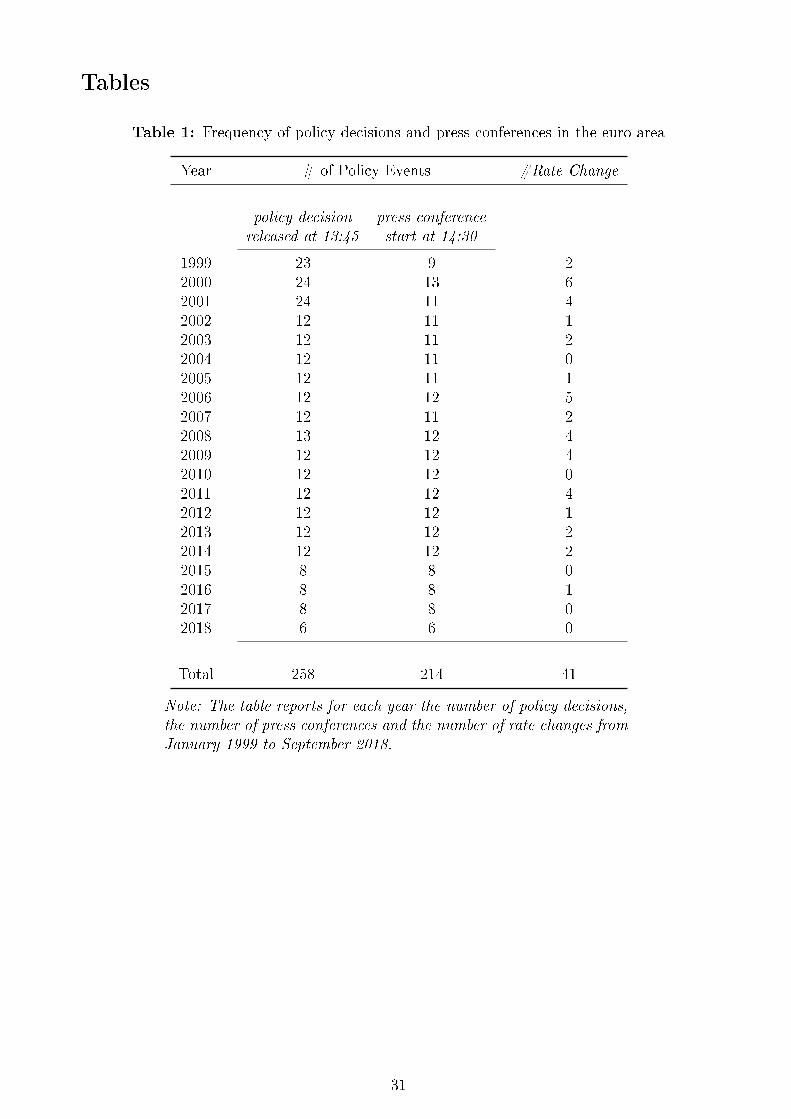
Tables

Table 1: Frequency of policy decisions and press conferences in the euro area

Year # of Policy Events #Rate Change

policy decision press conferencereleased at 13:45 start at 14:30

1999 23 9 22000 24 13 62001 24 11 42002 12 11 12003 12 11 22004 12 11 02005 12 11 12006 12 12 52007 12 11 22008 13 12 42009 12 12 42010 12 12 02011 12 12 42012 12 12 12013 12 12 22014 12 12 22015 8 8 02016 8 8 12017 8 8 02018 6 6 0

Total 258 214 41

Note: The table reports for each year the number of policy decisions,the number of press conferences and the number of rate changes fromJanuary 1999 to September 2018.

31

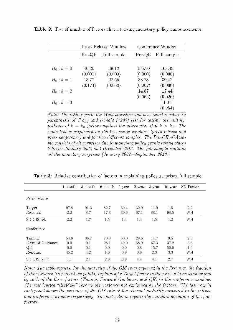
Table 2: Test of number of factors characterizing monetary policy announcements

Press Release Window Conference Window

Pre-QE Full sample Pre-QE Full sample

H0 : k = 0 46.20 49.12 105.50 108.49(0.001) (0.000) (0.000) (0.000)

H0 : k = 1 18.77 22.55 33.73 39.42(0.174) (0.068) (0.002) (0.000)

H0 : k = 2 14.87 17.44(0.062) (0.026)

H0 : k = 3 4.07(0.254)

Note: The table reports the Wald statistics and associated p-values inparenthesis of Cragg and Donald (1997) test for testing the null hy-pothesis of k = k0 factors against the alternative that k > k0. Thesame test is performed on the two policy windows (press release andpress conference) and for two di�erent samples. The Pre-QE sOAam-ple consists of all surprises due to monetary policy events taking placesbetween January 2002 and December 2013. The full sample containsall the monetary surprises (January 2002�September 2018).

Table 3: Relative contribution of factors in explaining policy surprises, full sample

1-month 3-month 6-month 1-year 2-year 5-year 10-year SD Factor

Press release

Target 97.8 91.3 82.7 60.4 32.9 11.9 1.5 2.2Residual 2.2 8.7 17.3 39.6 67.1 88.1 98.5 NA

SD OIS rel. 2.2 1.7 1.5 1.4 1.4 1.5 1.2 NA

Conference

Timing 54.8 86.7 70.3 50.0 29.6 14.7 9.5 2.3Forward Guidance 0.0 9.1 28.1 49.0 68.9 67.3 37.2 3.6QE 0.0 0.1 0.0 0.0 0.8 15.7 50.0 1.9Residual 45.2 4.2 1.6 0.9 0.8 2.3 3.3 NA

SD OIS conf. 1.1 2.1 2.8 3.9 4.4 4.1 2.7 NA

Note: The table reports, for the maturity of the OIS rates reported in the �rst row, the fractionof the variance (in percentage points) explained by Target factor in the press release window andby each of the three factors (Timing, Forward Guidance, and QE) in the conference window.The row labeled �Residual� reports the variance not explained by the factors. The last row ineach panel shows the variance of the OIS rate at the relevant maturity measured in the releaseand conference window respectively. The last column reports the standard deviation of the fourfactors.

32

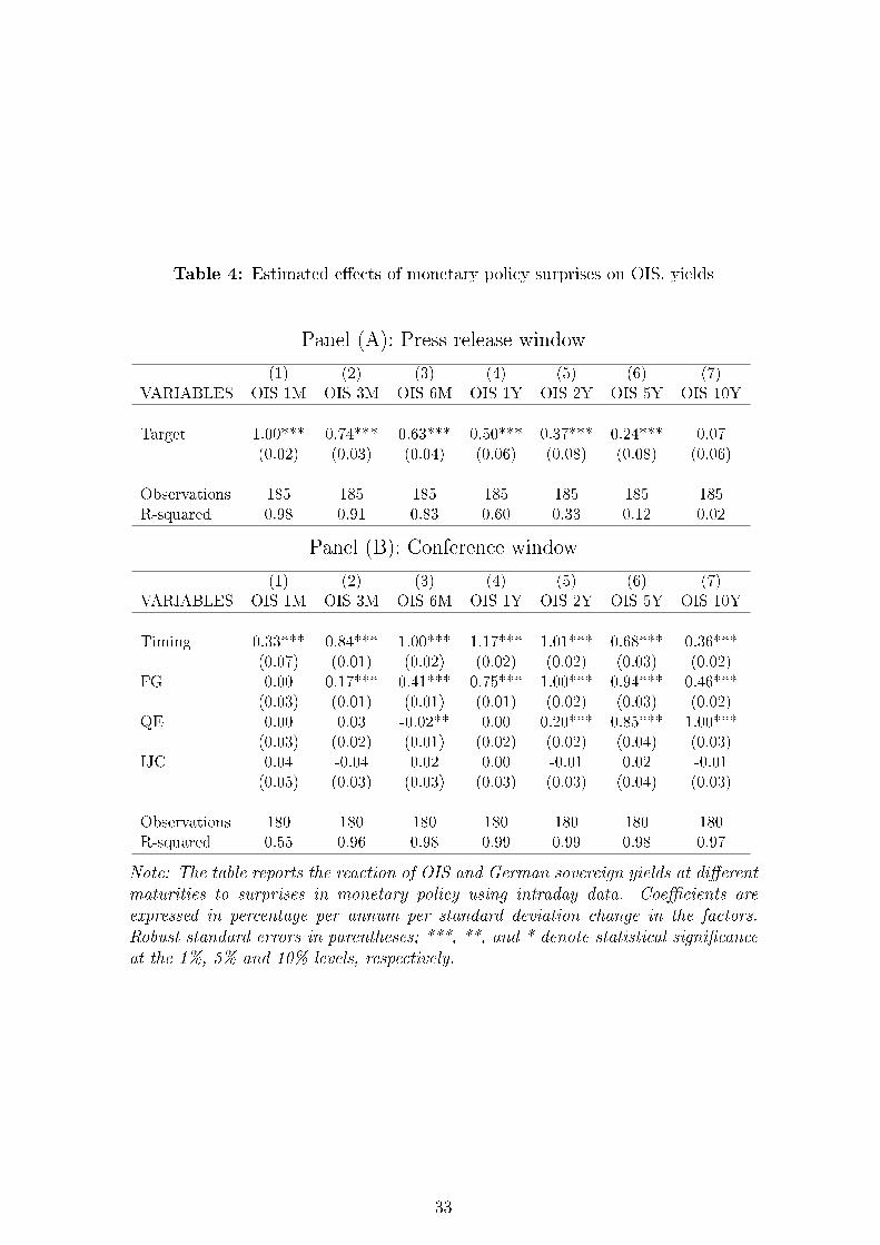
Table 4: Estimated e�ects of monetary policy surprises on OIS. yields

Panel (A): Press release window

(1) (2) (3) (4) (5) (6) (7)

VARIABLES OIS 1M OIS 3M OIS 6M OIS 1Y OIS 2Y OIS 5Y OIS 10Y

Target 1.00*** 0.74*** 0.63*** 0.50*** 0.37*** 0.24*** 0.07

(0.02) (0.03) (0.04) (0.06) (0.08) (0.08) (0.06)

Observations 185 185 185 185 185 185 185

R-squared 0.98 0.91 0.83 0.60 0.33 0.12 0.02

Panel (B): Conference window

(1) (2) (3) (4) (5) (6) (7)

VARIABLES OIS 1M OIS 3M OIS 6M OIS 1Y OIS 2Y OIS 5Y OIS 10Y

Timing 0.33*** 0.84*** 1.00*** 1.17*** 1.01*** 0.68*** 0.36***

(0.07) (0.01) (0.02) (0.02) (0.02) (0.03) (0.02)

FG 0.00 0.17*** 0.41*** 0.75*** 1.00*** 0.94*** 0.46***

(0.03) (0.01) (0.01) (0.01) (0.02) (0.03) (0.02)

QE 0.00 0.03 -0.02** 0.00 0.20*** 0.85*** 1.00***

(0.03) (0.02) (0.01) (0.02) (0.02) (0.04) (0.03)

IJC 0.04 -0.04 0.02 0.00 -0.01 0.02 -0.01

(0.05) (0.03) (0.03) (0.03) (0.03) (0.04) (0.03)

Observations 180 180 180 180 180 180 180

R-squared 0.55 0.96 0.98 0.99 0.99 0.98 0.97

Note: The table reports the reaction of OIS and German sovereign yields at di�erentmaturities to surprises in monetary policy using intraday data. Coe�cients areexpressed in percentage per annum per standard deviation change in the factors.Robust standard errors in parentheses; ***, **, and * denote statistical signi�canceat the 1%, 5% and 10% levels, respectively.

33

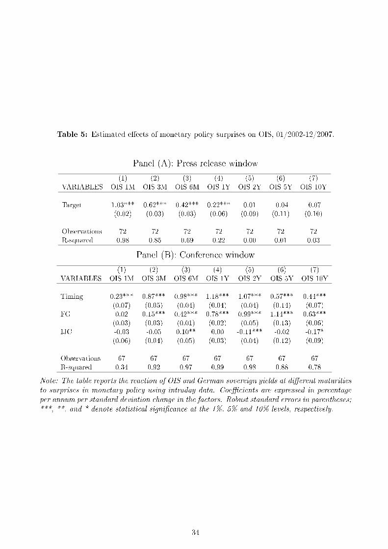
Table 5: Estimated e�ects of monetary policy surprises on OIS, 01/2002-12/2007.

Panel (A): Press release window

(1) (2) (3) (4) (5) (6) (7)

VARIABLES OIS 1M OIS 3M OIS 6M OIS 1Y OIS 2Y OIS 5Y OIS 10Y

Target 1.03*** 0.62*** 0.42*** 0.22*** 0.01 -0.04 -0.07

(0.02) (0.03) (0.03) (0.06) (0.09) (0.11) (0.10)

Observations 72 72 72 72 72 72 72

R-squared 0.98 0.85 0.69 0.22 0.00 0.01 0.03

Panel (B): Conference window

(1) (2) (3) (4) (5) (6) (7)

VARIABLES OIS 1M OIS 3M OIS 6M OIS 1Y OIS 2Y OIS 5Y OIS 10Y

Timing 0.23*** 0.87*** 0.98*** 1.18*** 1.07*** 0.57*** 0.44***

(0.07) (0.05) (0.04) (0.04) (0.04) (0.14) (0.07)

FG 0.02 0.15*** 0.42*** 0.78*** 0.99*** 1.14*** 0.63***

(0.03) (0.03) (0.01) (0.02) (0.05) (0.13) (0.06)

IJC -0.03 -0.05 0.10** 0.00 -0.11*** -0.02 -0.17*

(0.06) (0.04) (0.05) (0.03) (0.04) (0.12) (0.09)

Observations 67 67 67 67 67 67 67

R-squared 0.34 0.92 0.97 0.99 0.98 0.88 0.78

Note: The table reports the reaction of OIS and German sovereign yields at di�erent maturitiesto surprises in monetary policy using intraday data. Coe�cients are expressed in percentageper annum per standard deviation change in the factors. Robust standard errors in parentheses;***, **, and * denote statistical signi�cance at the 1%, 5% and 10% levels, respectively.

34

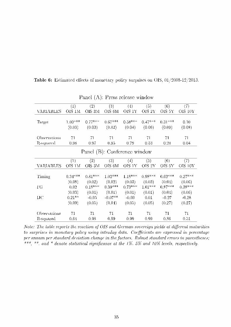
Table 6: Estimated e�ects of monetary policy surprises on OIS, 01/2008-12/2013.

Panel (A): Press release window

(1) (2) (3) (4) (5) (6) (7)

VARIABLES OIS 1M OIS 3M OIS 6M OIS 1Y OIS 2Y OIS 5Y OIS 10Y

Target 1.00*** 0.77*** 0.67*** 0.58*** 0.47*** 0.31*** 0.10

(0.03) (0.03) (0.02) (0.04) (0.06) (0.09) (0.08)

Observations 71 71 71 71 71 71 71

R-squared 0.98 0.97 0.95 0.79 0.53 0.20 0.04

Panel (B): Conference window

(1) (2) (3) (4) (5) (6) (7)

VARIABLES OIS 1M OIS 3M OIS 6M OIS 1Y OIS 2Y OIS 5Y OIS 10Y

Timing 0.34*** 0.81*** 1.02*** 1.18*** 0.98*** 0.62*** 0.27***

(0.08) (0.02) (0.02) (0.03) (0.03) (0.04) (0.06)

FG 0.02 0.18*** 0.39*** 0.73*** 1.01*** 0.87*** 0.38***

(0.03) (0.01) (0.01) (0.01) (0.01) (0.04) (0.06)

IJC 0.21** -0.05 -0.07** -0.00 0.01 -0.27 -0.28

(0.09) (0.05) (0.04) (0.05) (0.05) (0.27) (0.27)

Observations 71 71 71 71 71 71 71

R-squared 0.64 0.98 0.99 0.99 0.99 0.86 0.51

Note: The table reports the reaction of OIS and German sovereign yields at di�erent maturitiesto surprises in monetary policy using intraday data. Coe�cients are expressed in percentageper annum per standard deviation change in the factors. Robust standard errors in parentheses;***, **, and * denote statistical signi�cance at the 1%, 5% and 10% levels, respectively.

35

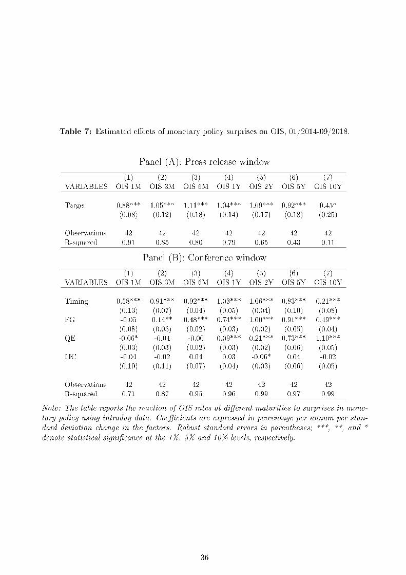
Table 7: Estimated e�ects of monetary policy surprises on OIS, 01/2014-09/2018.

Panel (A): Press release window

(1) (2) (3) (4) (5) (6) (7)

VARIABLES OIS 1M OIS 3M OIS 6M OIS 1Y OIS 2Y OIS 5Y OIS 10Y

Target 0.88*** 1.05*** 1.11*** 1.04*** 1.09*** 0.92*** 0.45*

(0.08) (0.12) (0.18) (0.14) (0.17) (0.18) (0.25)

Observations 42 42 42 42 42 42 42

R-squared 0.91 0.85 0.80 0.79 0.65 0.43 0.11

Panel (B): Conference window

(1) (2) (3) (4) (5) (6) (7)

VARIABLES OIS 1M OIS 3M OIS 6M OIS 1Y OIS 2Y OIS 5Y OIS 10Y

Timing 0.58*** 0.91*** 0.92*** 1.03*** 1.06*** 0.83*** 0.21***

(0.13) (0.07) (0.04) (0.05) (0.04) (0.10) (0.08)

FG -0.05 0.14** 0.48*** 0.74*** 1.00*** 0.91*** 0.49***

(0.08) (0.05) (0.02) (0.03) (0.02) (0.05) (0.04)

QE -0.06* -0.04 -0.00 0.09*** 0.21*** 0.73*** 1.10***

(0.03) (0.03) (0.02) (0.03) (0.02) (0.06) (0.05)

IJC -0.04 -0.02 0.04 0.03 -0.06* 0.04 -0.02

(0.10) (0.11) (0.07) (0.04) (0.03) (0.06) (0.05)

Observations 42 42 42 42 42 42 42

R-squared 0.71 0.87 0.95 0.96 0.99 0.97 0.99

Note: The table reports the reaction of OIS rates at di�erent maturities to surprises in mone-tary policy using intraday data. Coe�cients are expressed in percentage per annum per stan-dard deviation change in the factors. Robust standard errors in parentheses; ***, **, and *denote statistical signi�cance at the 1%, 5% and 10% levels, respectively.

36

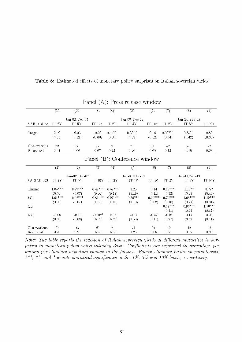
Table 8: Estimated e�ects of monetary policy surprises on Italian sovereign yields

Panel (A): Press release window

(1) (2) (3) (4) (5) (6) (7) (8) (9)

Jan-02/Dec-07 Jan-08/Dec-13 Jan-14/Sep-18VARIABLES IT 2Y IT 5Y IT 10Y IT 2Y IT 5Y IT 10Y IT 2Y IT 5Y IT 10Y

Target 0.10 -0.03 -0.06 0.45** 0.39** 0.16 0.99*** 0.85** 0.80(0.11) (0.12) (0.09) (0.20) (0.19) (0.12) (0.34) (0.42) (0.62)

Observations 72 72 72 71 71 71 42 42 42R-squared 0.04 0.00 0.03 0.22 0.16 0.05 0.12 0.10 0.08

Panel (B): Conference window

(1) (2) (3) (4) (5) (6) (7) (8) (9)

Jan-02/Dec-07 Jan-08/Dec-13 Jan-14/Sep-18VARIABLES IT 2Y IT 5Y IT 10Y IT 2Y IT 5Y IT 10Y IT 2Y IT 5Y IT 10Y

Timing 1.05*** 0.77*** 0.42*** 0.62*** 0.25 0.14 0.89*** 1.19** 0.77*(0.06) (0.07) (0.06) (0.18) (0.19) (0.11) (0.32) (0.48) (0.46)

FG 1.01*** 0.92*** 0.61*** 0.97*** 0.76*** 0.29*** 0.76*** 1.08*** 1.12***(0.06) (0.07) (0.06) (0.10) (0.10) (0.08) (0.16) (0.27) (0.31)

QE 0.57*** 0.96*** 1.76***(0.11) (0.24) (0.17)

IJC -0.09 -0.15 -0.20** 0.05 -0.57 -0.57 -0.08 0.17 0.06(0.06) (0.09) (0.09) (0.49) (0.59) (0.41) (0.27) (0.42) (0.41)

Observations 67 67 67 71 71 71 42 42 42R-squared 0.96 0.91 0.78 0.43 0.26 0.08 0.71 0.69 0.80

Note: The table reports the reaction of Italian sovereign yields at di�erent maturities to sur-prises in monetary policy using intraday data. Coe�cients are expressed in percentage perannum per standard deviation change in the factors. Robust standard errors in parentheses;***, **, and * denote statistical signi�cance at the 1%, 5% and 10% levels, respectively.

37

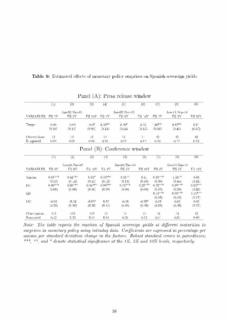
Table 9: Estimated e�ects of monetary policy surprises on Spanish sovereign yields

Panel (A): Press release window

(1) (2) (3) (4) (5) (6) (7) (8) (9)

Jan-02/Dec-07 Jan-08/Dec-13 Jan-14/Sep-18VARIABLES ES 2Y ES 5Y ES 10Y ES 2Y ES 5Y ES 10Y ES 2Y ES 5Y ES 10Y

Target 0.06 -0.04 -0.07 0.39** 0.26* 0.25 1.00*** 0.87** 0.81(0.10) (0.12) (0.09) (0.18) (0.14) (0.15) (0.33) (0.41) (0.67)

Observations 72 72 72 71 71 71 42 42 42R-squared 0.02 0.01 0.03 0.16 0.11 0.12 0.43 0.22 0.10

Panel (B): Conference window

(1) (2) (3) (4) (5) (6) (7) (8) (9)

Jan-02/Dec-07 Jan-08/Dec-13 Jan-14/Sep-18VARIABLES ES 2Y ES 5Y ES 10Y ES 2Y ES 5Y ES 10Y ES 2Y ES 5Y ES 10Y

Timing 0.61*** 0.41*** 0.21* 0.53*** 0.31** 0.11 0.93*** 1.18** 0.68(0.12) (0.14) (0.11) (0.12) (0.13) (0.10) (0.30) (0.44) (0.41)

FG 0.86*** 0.69*** 0.34*** 0.90*** 0.71*** 0.32*** 0.72*** 0.99*** 0.95***(0.09) (0.08) (0.08) (0.09) (0.08) (0.08) (0.15) (0.26) (0.26)

QE 0.54*** 0.68*** 1.45***(0.10) (0.13) (0.17)

IJC -0.02 -0.52 -0.69* 0.07 -0.50 -0.70* 0.19 0.02 0.03(0.33) (0.38) (0.36) (0.41) (0.46) (0.40) (0.23) (0.40) (0.37)

Observations 113 113 113 71 71 71 42 42 42R-squared 0.52 0.33 0.11 0.54 0.35 0.12 0.74 0.67 0.80

Note: The table reports the reaction of Spanish sovereign yields at di�erent maturities tosurprises in monetary policy using intraday data. Coe�cients are expressed in percentage perannum per standard deviation change in the factors. Robust standard errors in parentheses;***, **, and * denote statistical signi�cance at the 1%, 5% and 10% levels, respectively.

38

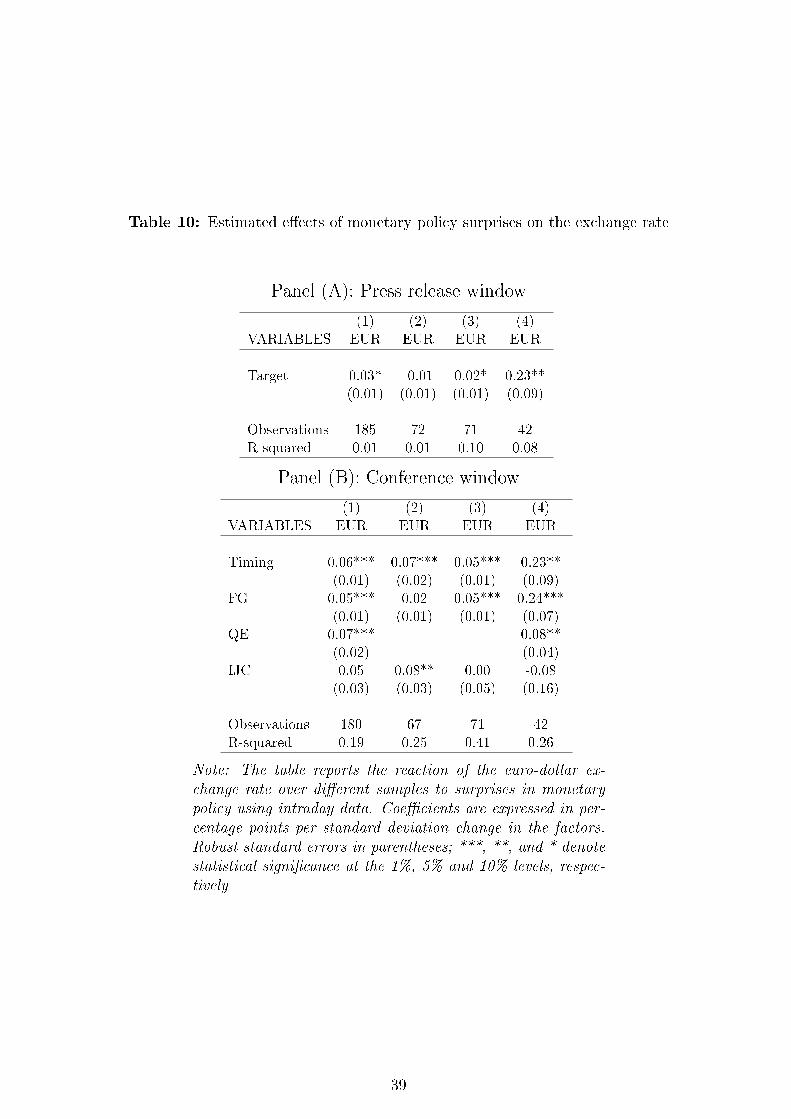
Table 10: Estimated e�ects of monetary policy surprises on the exchange rate

Panel (A): Press release window

(1) (2) (3) (4)

VARIABLES EUR EUR EUR EUR

Target 0.03* -0.01 0.02* 0.23**

(0.01) (0.01) (0.01) (0.09)

Observations 185 72 71 42

R-squared 0.01 0.01 0.10 0.08

Panel (B): Conference window

(1) (2) (3) (4)

VARIABLES EUR EUR EUR EUR

Timing 0.06*** 0.07*** 0.05*** 0.23**

(0.01) (0.02) (0.01) (0.09)

FG 0.05*** 0.02 0.05*** 0.24***

(0.01) (0.01) (0.01) (0.07)

QE 0.07*** 0.08**

(0.02) (0.04)

IJC 0.05 0.08** 0.00 -0.08

(0.03) (0.03) (0.05) (0.16)

Observations 180 67 71 42

R-squared 0.19 0.25 0.41 0.26

Note: The table reports the reaction of the euro-dollar ex-change rate over di�erent samples to surprises in monetarypolicy using intraday data. Coe�cients are expressed in per-centage points per standard deviation change in the factors.Robust standard errors in parentheses; ***, **, and * denotestatistical signi�cance at the 1%, 5% and 10% levels, respec-tively

39

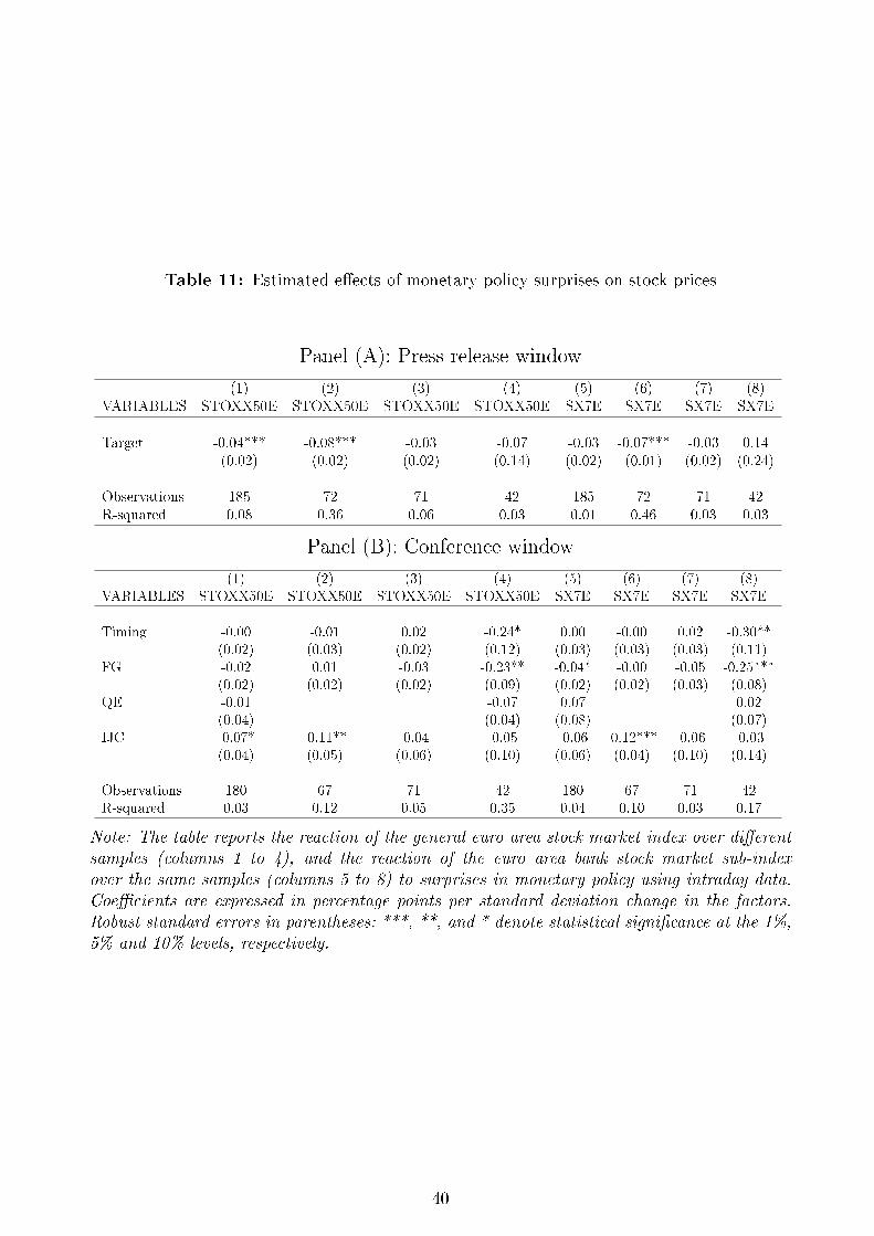
Table 11: Estimated e�ects of monetary policy surprises on stock prices

Panel (A): Press release window

(1) (2) (3) (4) (5) (6) (7) (8)VARIABLES STOXX50E STOXX50E STOXX50E STOXX50E SX7E SX7E SX7E SX7E

Target -0.04*** -0.08*** -0.03 -0.07 -0.03 -0.07*** -0.03 0.14(0.02) (0.02) (0.02) (0.14) (0.02) (0.01) (0.02) (0.24)

Observations 185 72 71 42 185 72 71 42R-squared 0.08 0.36 0.06 0.03 0.01 0.46 0.03 0.03

Panel (B): Conference window

(1) (2) (3) (4) (5) (6) (7) (8)VARIABLES STOXX50E STOXX50E STOXX50E STOXX50E SX7E SX7E SX7E SX7E

Timing -0.00 -0.01 0.02 -0.24* 0.00 -0.00 0.02 -0.30**(0.02) (0.03) (0.02) (0.12) (0.03) (0.03) (0.03) (0.11)

FG -0.02 0.01 -0.03 -0.23** -0.04* -0.00 -0.05 -0.25***(0.02) (0.02) (0.02) (0.09) (0.02) (0.02) (0.03) (0.08)

QE -0.01 -0.07 0.07 0.02(0.04) (0.04) (0.08) (0.07)

IJC -0.07* -0.11** -0.04 -0.05 -0.06 -0.12*** -0.06 -0.03(0.04) (0.05) (0.06) (0.10) (0.06) (0.04) (0.10) (0.14)

Observations 180 67 71 42 180 67 71 42R-squared 0.03 0.12 0.05 0.35 0.04 0.10 0.03 0.17

Note: The table reports the reaction of the general euro area stock market index over di�erentsamples (columns 1 to 4), and the reaction of the euro area bank stock market sub-indexover the same samples (columns 5 to 8) to surprises in monetary policy using intraday data.Coe�cients are expressed in percentage points per standard deviation change in the factors.Robust standard errors in parentheses; ***, **, and * denote statistical signi�cance at the 1%,5% and 10% levels, respectively.

40

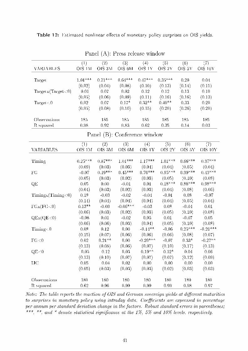
Table 12: Estimated nonlinear e�ects of monetary policy surprises on OIS yields.

Panel (A): Press release window

(1) (2) (3) (4) (5) (6) (7)

VARIABLES OIS 1M OIS 3M OIS 6M OIS 1Y OIS 2Y OIS 5Y OIS 10Y

Target 1.01*** 0.71*** 0.64*** 0.47*** 0.35*** 0.20 0.04

(0.02) (0.04) (0.08) (0.10) (0.13) (0.14) (0.11)

Targetx(Target<0) -0.01 0.07 0.02 0.12 0.12 0.13 0.10

(0.05) (0.06) (0.09) (0.11) (0.16) (0.16) (0.13)

Target<0 0.02 0.07 0.17* 0.32** 0.40** 0.33 0.20

(0.05) (0.08) (0.10) (0.15) (0.20) (0.26) (0.20)

Observations 185 185 185 185 185 185 185

R-squared 0.98 0.92 0.83 0.62 0.35 0.14 0.03

Panel (B): Conference window

(1) (2) (3) (4) (5) (6) (7)

VARIABLES OIS 1M OIS 3M OIS 6M OIS 1Y OIS 2Y OIS 5Y OIS 10Y

Timing 0.25*** 0.87*** 1.01*** 1.17*** 1.01*** 0.66*** 0.37***

(0.09) (0.03) (0.03) (0.04) (0.04) (0.05) (0.04)

FG -0.07 0.19*** 0.45*** 0.76*** 0.95*** 0.99*** 0.43***

(0.05) (0.03) (0.02) (0.03) (0.05) (0.10) (0.08)

QE 0.05 0.00 -0.01 0.01 0.18*** 0.88*** 0.98***

(0.04) (0.03) (0.02) (0.03) (0.04) (0.08) (0.06)

Timingx(Timing<0) 0.18 -0.03 -0.02 -0.04 -0.01 0.08 -0.07

(0.14) (0.04) (0.04) (0.04) (0.04) (0.05) (0.04)

FGx(FG<0) 0.13** -0.00 -0.06*** -0.03 0.08 -0.04 0.01

(0.06) (0.03) (0.02) (0.03) (0.05) (0.10) (0.08)

QEx(QE<0) -0.08 0.01 -0.02 0.05 0.01 -0.07 0.05

(0.06) (0.06) (0.03) (0.04) (0.05) (0.10) (0.08)

Timing<0 0.08 0.12 0.00 -0.14** -0.06 0.25*** -0.21***

(0.15) (0.07) (0.06) (0.06) (0.06) (0.08) (0.07)

FG<0 0.02 0.21** 0.00 -0.20*** -0.07 0.33* -0.27**

(0.13) (0.08) (0.06) (0.07) (0.10) (0.17) (0.13)

QE<0 -0.05 -0.12 0.03 0.19** -0.12* -0.04 0.06

(0.13) (0.10) (0.07) (0.07) (0.07) (0.12) (0.09)

IJC 0.05 -0.04 0.02 0.00 -0.00 -0.00 0.00

(0.05) (0.03) (0.03) (0.03) (0.02) (0.03) (0.03)

Observations 180 180 180 180 180 180 180

R-squared 0.62 0.96 0.99 0.99 0.99 0.98 0.97

Note: The table reports the reaction of OIS and German sovereign yields at di�erent maturitiesto surprises in monetary policy using intraday data. Coe�cients are expressed in percentageper annum per standard deviation change in the factors. Robust standard errors in parentheses;***, **, and * denote statistical signi�cance at the 1%, 5% and 10% levels, respectively.

41

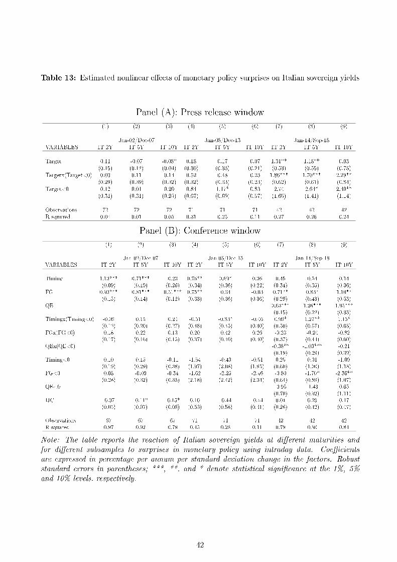
Table 13: Estimated nonlinear e�ects of monetary policy surprises on Italian sovereign yields

Panel (A): Press release window

(1) (2) (3) (4) (5) (6) (7) (8) (9)

Jan-02/Dec-07 Jan-08/Dec-13 Jan-14/Sep-18VARIABLES IT 2Y IT 5Y IT 10Y IT 2Y IT 5Y IT 10Y IT 2Y IT 5Y IT 10Y

Target 0.11 -0.07 -0.08* 0.18 0.17 0.07 1.31** 1.18** 0.93(0.15) (0.12) (0.04) (0.30) (0.33) (0.21) (0.53) (0.55) (0.78)

Targetx(Target<0) 0.03 0.11 0.14 0.52 0.48 0.23 1.86*** 1.70*** 2.29**(0.29) (0.39) (0.32) (0.32) (0.33) (0.23) (0.62) (0.61) (0.84)

Target<0 0.12 0.01 0.20 0.84 1.17* 0.83 2.74 2.64* 2.40**(0.31) (0.31) (0.25) (0.67) (0.69) (0.57) (1.65) (1.41) (1.14)

Observations 72 72 72 71 71 71 42 42 42R-squared 0.04 0.01 0.05 0.31 0.25 0.11 0.27 0.26 0.24

Panel (B): Conference window

(1) (2) (3) (4) (5) (6) (7) (8) (9)

Jan-02/Dec-07 Jan-08/Dec-13 Jan-14/Sep-18VARIABLES IT 2Y IT 5Y IT 10Y IT 2Y IT 5Y IT 10Y IT 2Y IT 5Y IT 10Y

Timing 1.13*** 0.71*** 0.23 0.76** 0.69* 0.36 0.45 0.54 0.14(0.09) (0.19) (0.26) (0.34) (0.36) (0.22) (0.34) (0.35) (0.36)

FG 0.93*** 0.81*** 0.51*** 0.75** 0.34 -0.03 0.71** 0.83* 1.10**(0.15) (0.14) (0.12) (0.33) (0.36) (0.36) (0.29) (0.43) (0.53)

QE 0.63*** 1.26*** 1.95***(0.15) (0.22) (0.33)

Timingx(Timing<0) -0.09 0.15 0.24 -0.51 -0.83* -0.46 0.99* 1.27** 1.15*(0.12) (0.20) (0.27) (0.48) (0.45) (0.30) (0.50) (0.57) (0.68)

FGx(FG<0) 0.18 0.22 0.13 0.20 0.42 0.26 -0.23 -0.24 -0.82(0.17) (0.16) (0.15) (0.37) (0.40) (0.40) (0.37) (0.44) (0.60)

QEx(QE<0) -0.38** -1.03*** -0.21(0.19) (0.29) (0.39)

Timing<0 0.10 0.15 -0.11 -1.54 -0.43 -0.51 0.25 0.01 -1.09(0.19) (0.29) (0.38) (1.97) (2.08) (1.95) (0.60) (1.00) (1.18)

FG<0 0.08 -0.09 -0.34 -1.62 -2.25 -2.46 -0.80 -1.70* -2.36**(0.28) (0.32) (0.35) (2.18) (2.42) (2.34) (0.64) (0.89) (1.07)

QE<0 -0.95 -1.43 0.65(0.70) (0.92) (1.11)

IJC -0.07 -0.11* -0.15* 0.10 -0.44 -0.44 0.04 0.29 0.17(0.05) (0.07) (0.08) (0.53) (0.58) (0.41) (0.26) (0.42) (0.47)

Observations 67 67 67 71 71 71 42 42 42R-squared 0.97 0.92 0.79 0.45 0.28 0.11 0.79 0.80 0.84

Note: The table reports the reaction of Italian sovereign yields at di�erent maturities andfor di�erent subsamples to surprises in monetary policy using intraday data. Coe�cientsare expressed in percentage per annum per standard deviation change in the factors. Robuststandard errors in parentheses; ***, **, and * denote statistical signi�cance at the 1%, 5%and 10% levels, respectively.

42

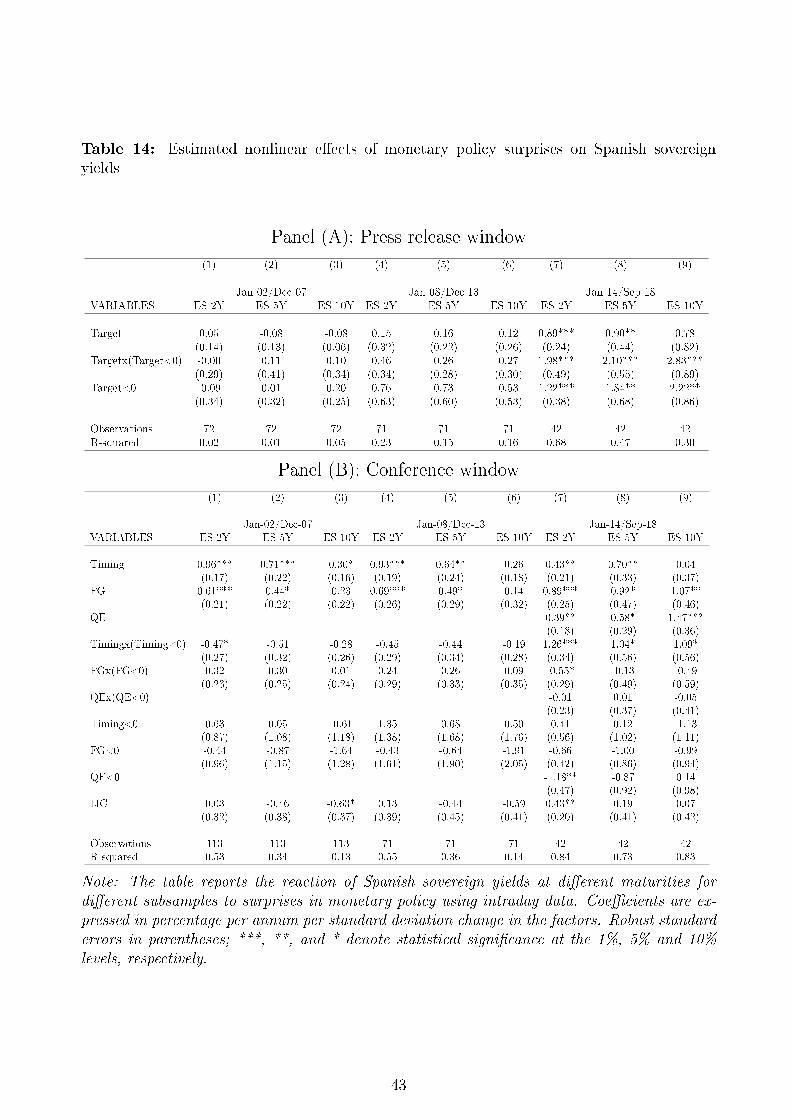
Table 14: Estimated nonlinear e�ects of monetary policy surprises on Spanish sovereignyields

Panel (A): Press release window

(1) (2) (3) (4) (5) (6) (7) (8) (9)

Jan-02/Dec-07 Jan-08/Dec-13 Jan-14/Sep-18VARIABLES ES 2Y ES 5Y ES 10Y ES 2Y ES 5Y ES 10Y ES 2Y ES 5Y ES 10Y

Target 0.05 -0.08 -0.08 0.15 0.16 0.12 0.89*** 0.90** 0.78(0.14) (0.13) (0.06) (0.32) (0.22) (0.26) (0.24) (0.44) (0.82)

Targetx(Target<0) -0.00 0.11 0.10 0.46 0.26 0.27 1.98*** 2.10*** 2.83***(0.29) (0.41) (0.34) (0.34) (0.28) (0.30) (0.49) (0.55) (0.89)

Target<0 -0.09 0.01 0.20 0.76 0.73 0.53 1.22*** 1.84** 2.22**(0.34) (0.32) (0.25) (0.63) (0.60) (0.53) (0.38) (0.68) (0.86)

Observations 72 72 72 71 71 71 42 42 42R-squared 0.02 0.01 0.05 0.23 0.15 0.16 0.68 0.47 0.30

Panel (B): Conference window

(1) (2) (3) (4) (5) (6) (7) (8) (9)

Jan-02/Dec-07 Jan-08/Dec-13 Jan-14/Sep-18VARIABLES ES 2Y ES 5Y ES 10Y ES 2Y ES 5Y ES 10Y ES 2Y ES 5Y ES 10Y

Timing 0.96*** 0.71*** 0.30* 0.93*** 0.64** 0.26 0.43** 0.70** 0.04(0.17) (0.22) (0.16) (0.19) (0.24) (0.18) (0.21) (0.33) (0.37)

FG 0.61*** 0.44* 0.23 0.69*** 0.49* 0.14 0.89*** 0.92* 1.07**(0.21) (0.22) (0.22) (0.26) (0.29) (0.32) (0.25) (0.47) (0.46)

QE 0.39** 0.58* 1.47***(0.18) (0.29) (0.36)

Timingx(Timing<0) -0.47* -0.51 -0.28 -0.45 -0.44 -0.19 1.26*** 1.04* 1.09*(0.27) (0.32) (0.26) (0.29) (0.34) (0.28) (0.34) (0.56) (0.56)

FGx(FG<0) 0.32 0.30 0.01 0.24 0.26 0.09 -0.55* -0.13 -0.49(0.23) (0.25) (0.24) (0.29) (0.33) (0.35) (0.29) (0.49) (0.59)

QEx(QE<0) -0.01 0.01 -0.05(0.23) (0.37) (0.41)

Timing<0 0.63 0.05 -0.61 1.35 0.68 0.50 0.41 0.12 -1.13(0.87) (1.08) (1.18) (1.38) (1.68) (1.76) (0.56) (1.02) (1.11)

FG<0 -0.44 -0.87 -1.64 -0.43 -0.64 -1.91 -0.66 -1.00 -0.99(0.96) (1.15) (1.28) (1.61) (1.90) (2.05) (0.42) (0.86) (0.94)

QE<0 -1.18** -0.87 0.14(0.47) (0.92) (0.98)

IJC 0.03 -0.46 -0.63* 0.13 -0.44 -0.59 0.43** 0.19 0.07(0.32) (0.38) (0.37) (0.39) (0.45) (0.41) (0.20) (0.41) (0.42)

Observations 113 113 113 71 71 71 42 42 42R-squared 0.53 0.34 0.13 0.55 0.36 0.14 0.84 0.73 0.83

Note: The table reports the reaction of Spanish sovereign yields at di�erent maturities fordi�erent subsamples to surprises in monetary policy using intraday data. Coe�cients are ex-pressed in percentage per annum per standard deviation change in the factors. Robust standarderrors in parentheses; ***, **, and * denote statistical signi�cance at the 1%, 5% and 10%levels, respectively.

43

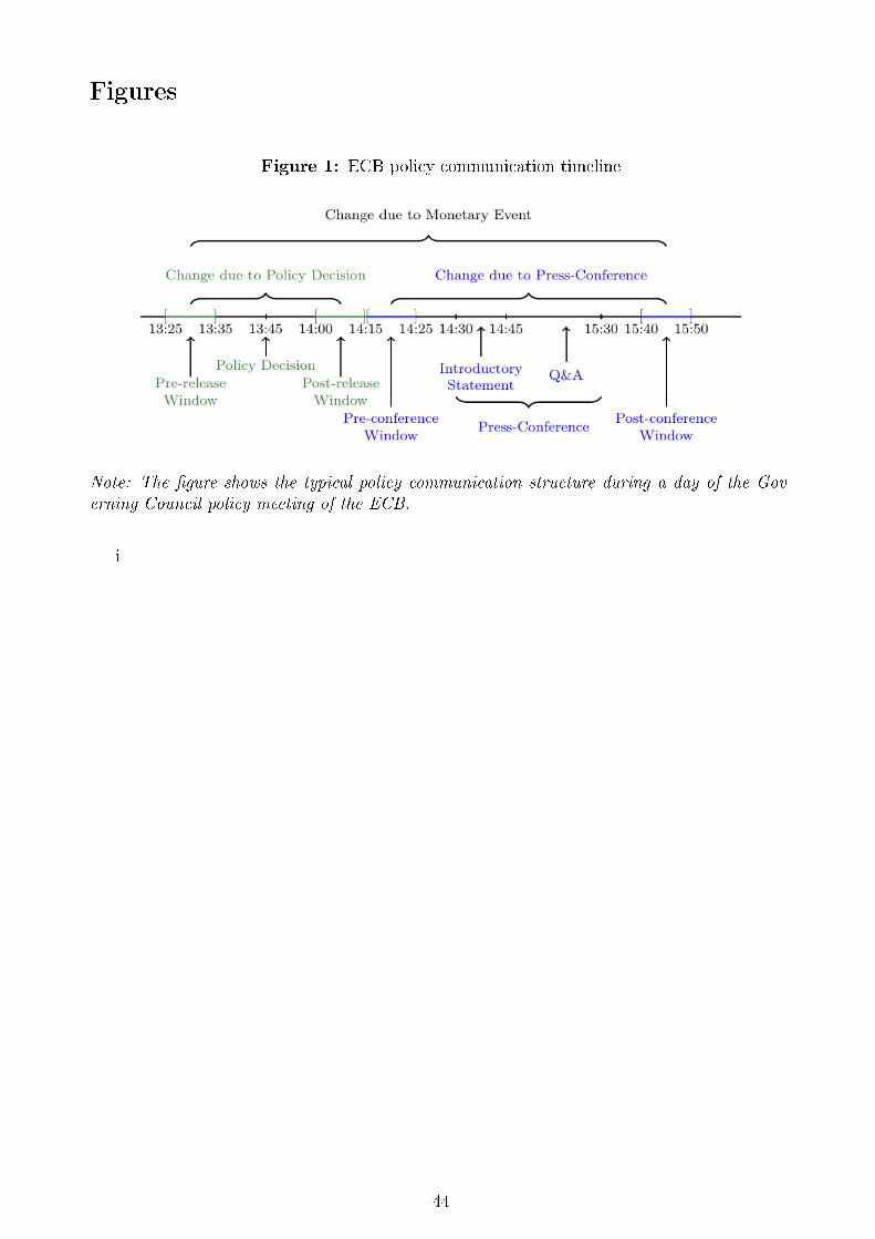
Figures

Figure 1: ECB policy communication timeline

Note: The �gure shows the typical policy communication structure during a day of the Gov-erning Council policy meeting of the ECB.

i

44

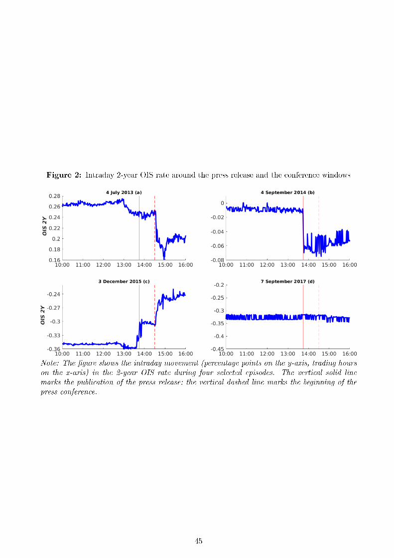
Figure 2: Intraday 2-year OIS rate around the press release and the conference windows

Note: The �gure shows the intraday movement (percentage points on the y-axis, trading hourson the x-axis) in the 2-year OIS rate during four selected episodes. The vertical solid linemarks the publication of the press release; the vertical dashed line marks the beginning of thepress conference.

45

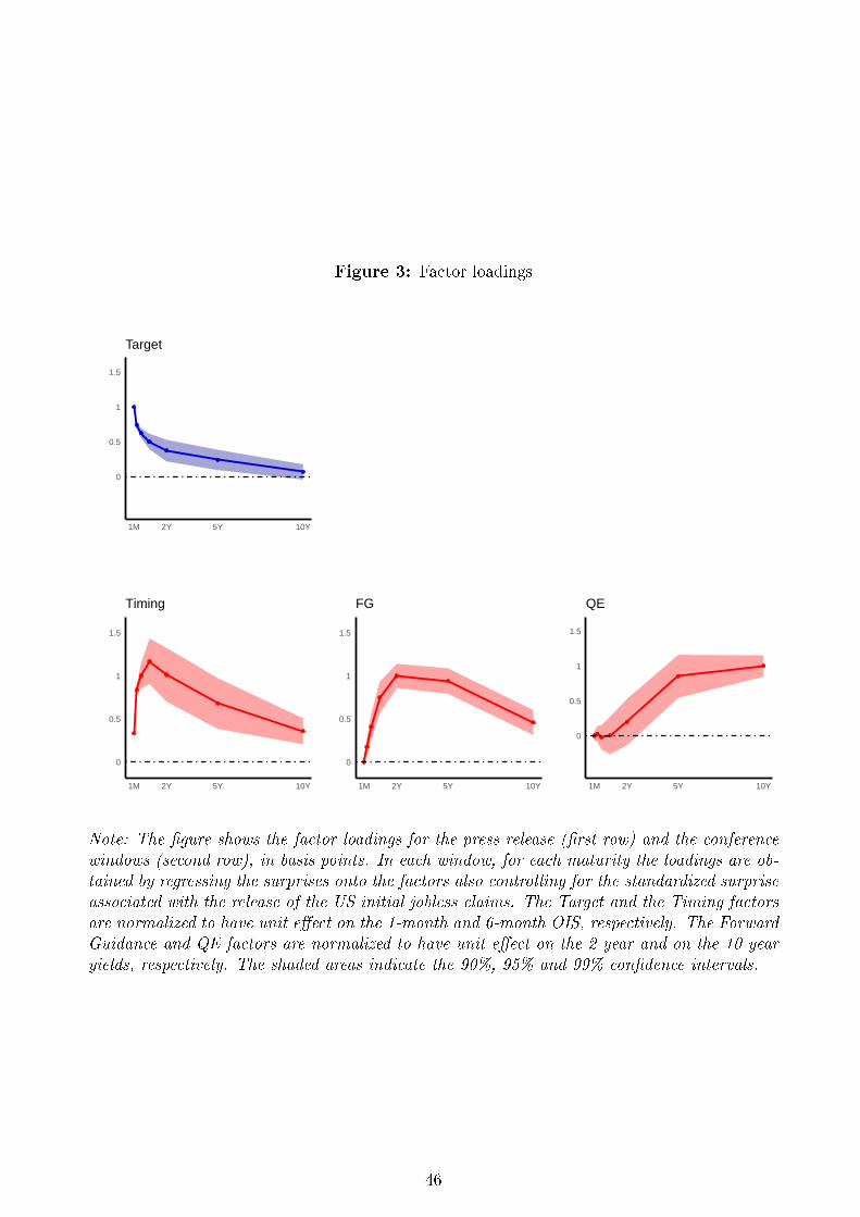
Figure 3: Factor loadings

0

0.5

1

1.5

1M 2Y 5Y 10Y

Target

0

0.5

1

1.5

1M 2Y 5Y 10Y

Timing

0

0.5

1

1.5

1M 2Y 5Y 10Y

FG

0

0.5

1

1.5

1M 2Y 5Y 10Y

QE

Note: The �gure shows the factor loadings for the press release (�rst row) and the conferencewindows (second row), in basis points. In each window, for each maturity the loadings are ob-tained by regressing the surprises onto the factors also controlling for the standardized surpriseassociated with the release of the US initial jobless claims. The Target and the Timing factorsare normalized to have unit e�ect on the 1-month and 6-month OIS, respectively. The ForwardGuidance and QE factors are normalized to have unit e�ect on the 2-year and on the 10-yearyields, respectively. The shaded areas indicate the 90%, 95% and 99% con�dence intervals.

46

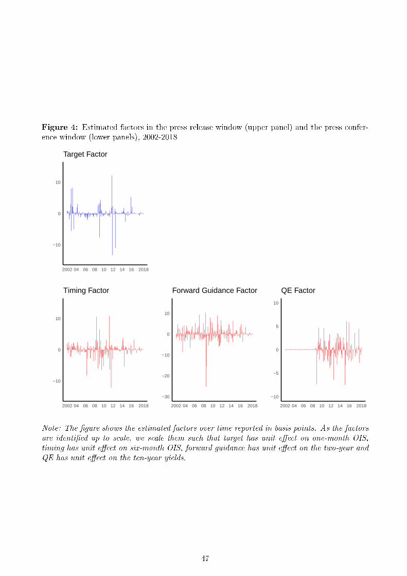
Figure 4: Estimated factors in the press release window (upper panel) and the press confer-ence window (lower panels), 2002-2018

−10

0

10

2002 04 06 08 10 12 14 16 2018

Target Factor

−10

0

10

2002 04 06 08 10 12 14 16 2018

Timing Factor

−30

−20

−10

0

10

2002 04 06 08 10 12 14 16 2018

Forward Guidance Factor

−10

−5

0

5

10

2002 04 06 08 10 12 14 16 2018

QE Factor

Note: The �gure shows the estimated factors over time reported in basis points. As the factorsare identi�ed up to scale, we scale them such that target has unit e�ect on one-month OIS,timing has unit e�ect on six-month OIS, forward guidance has unit e�ect on the two-year andQE has unit e�ect on the ten-year yields.

47

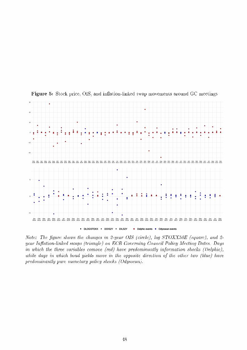
Figure 5: Stock price, OIS, and in�ation-linked swap movements around GC meetings

−20

−10

0

10

20

30

Feb2008

Mar2008

Apr2008

May2008

Jun2008

Aug2008

Oct2008

Jan2009

Feb2009

Mar2009

Apr2009

Jun2009

Jul2009

Aug2009

Sep2009

Oct2009

Nov2009

Dec2009

Jan2010

Mar2010

Apr2010

Jul2010

Sep2010

Oct2010

Nov2010

Dec2010

Jan2011

Feb2011

Mar2011

May2011

Jun2011

Jul2011

Aug2011

Sep2011

Dec2011

May2012

Jun2012

Jul2012

Dec2012

Jan2013

Feb2013

Mar2013

May2013

Jun2013

Jul2013

Aug2013

Oct2013

Dec2013

−5

0

5

Jan2014

Feb2014

Mar2014

Apr2014

May2014

Jun2014

Jul2014

Aug2014

Sep2014

Oct2014

Nov2014

Jan2015

Mar2015

Apr2015

Jun2015

Sep2015

Oct2015

Dec2015

Jan2016

Mar2016

Apr2016

Jun2016

Sep2016

Oct2016

Dec2016

Jan2017

Mar2017

Apr2017

Jun2017

Jul2017

Sep2017

Oct2017

Dec2017

Jan2018

Mar2018

Apr2018

Jun2018

Jul2018

Sep2018

DLOGSTOXX DOIS2Y DILS2Y Delphic events Odyssean events

−20

−10

0

10

20

30

Feb2008

Mar2008

Apr2008

May2008

Jun2008

Aug2008

Oct2008

Jan2009

Feb2009

Mar2009

Apr2009

Jun2009

Jul2009

Aug2009

Sep2009

Oct2009

Nov2009

Dec2009

Jan2010

Mar2010

Apr2010

Jul2010

Sep2010

Oct2010

Nov2010

Dec2010

Jan2011

Feb2011

Mar2011

May2011

Jun2011

Jul2011

Aug2011

Sep2011

Dec2011

May2012

Jun2012

Jul2012

Dec2012

Jan2013

Feb2013

Mar2013

May2013

Jun2013

Jul2013

Aug2013

Oct2013

Dec2013

−5

0

5

Jan2014

Feb2014

Mar2014

Apr2014

May2014

Jun2014

Jul2014

Aug2014

Sep2014

Oct2014

Nov2014

Jan2015

Mar2015

Apr2015

Jun2015

Sep2015

Oct2015

Dec2015

Jan2016

Mar2016

Apr2016

Jun2016

Sep2016

Oct2016

Dec2016

Jan2017

Mar2017

Apr2017

Jun2017

Jul2017

Sep2017

Oct2017

Dec2017

Jan2018

Mar2018

Apr2018

Jun2018

Jul2018

Sep2018

DLOGSTOXX DOIS2Y DILS2Y Delphic events Odyssean events

Note: The �gure shows the changes in 2-year OIS (circle), log STOXX50E (square), and 2-year In�ation-linked swaps (triangle) on ECB Governing Council Policy Meeting Dates. Daysin which the three variables comove (red) have predominantly information shocks (Delphic),while days in which bond yields move in the opposite direction of the other two (blue) havepredominantly pure monetary policy shocks (Odyssean).

48

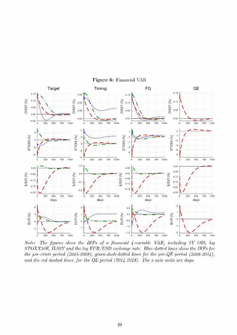
Figure 6: Financial VAR

Note: The �gures show the IRFs of a �nancial 4-variable VAR, including 2Y OIS, logSTOXX50E, ILS2Y and the log EUR/USD exchange rate. Blue-dotted lines show the IRFs forthe pre-crisis period (2005-2008), green-dash-dotted lines for the pre-QE period (2008-2014),and the red-dashed lines, for the QE period (2014-2018). The x-axis units are days.

49

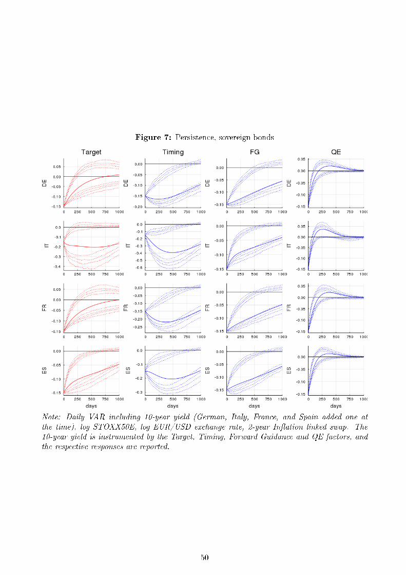
Figure 7: Persistence, sovereign bonds

Note: Daily VAR including 10-year yield (German, Italy, France, and Spain added one atthe time), log STOXX50E, log EUR/USD exchange rate, 2-year In�ation linked swap. The10-year yield is instrumented by the Target, Timing, Forward Guidance and QE factors, andthe respective responses are reported.

50

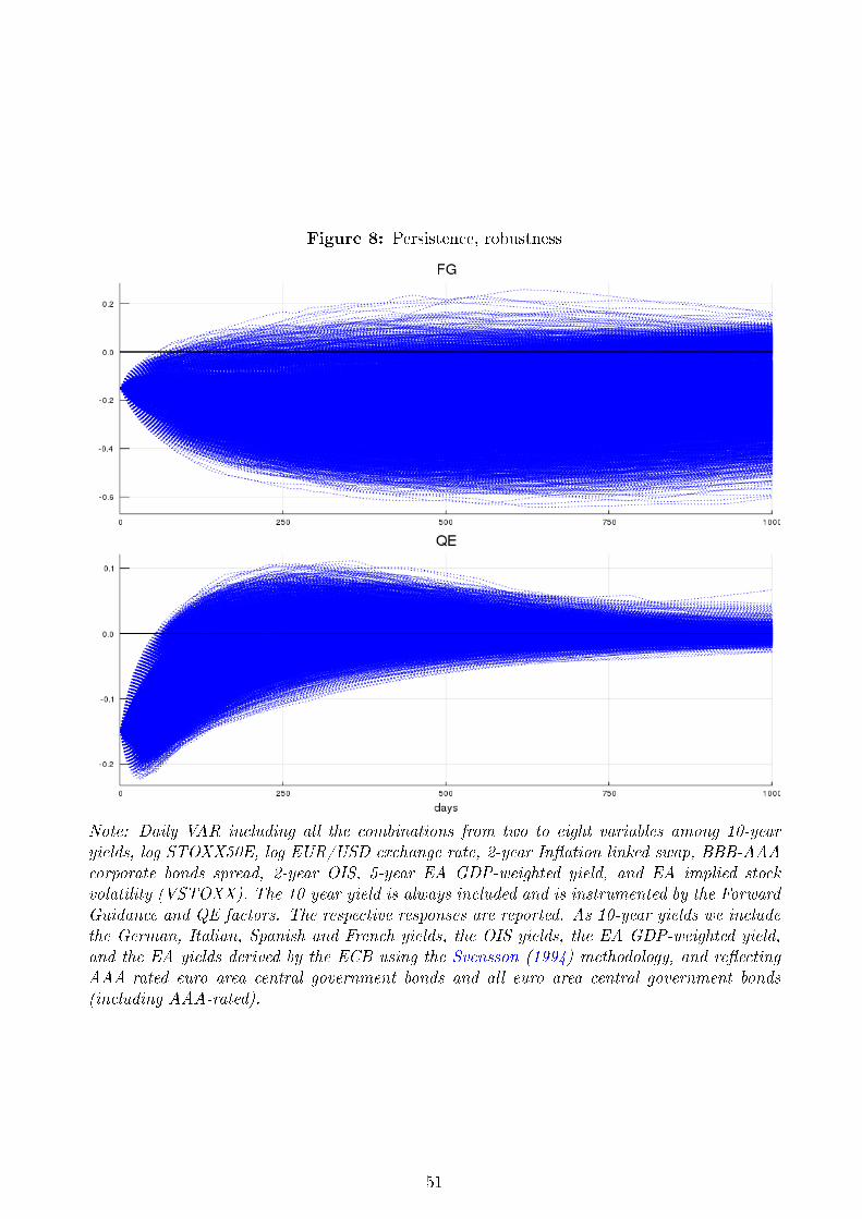
Figure 8: Persistence, robustness

Note: Daily VAR including all the combinations from two to eight variables among 10-yearyields, log STOXX50E, log EUR/USD exchange rate, 2-year In�ation linked swap, BBB-AAAcorporate bonds spread, 2-year OIS, 5-year EA GDP-weighted yield, and EA implied stockvolatility (VSTOXX). The 10-year yield is always included and is instrumented by the ForwardGuidance and QE factors. The respective responses are reported. As 10-year yields we includethe German, Italian, Spanish and French yields, the OIS yields, the EA GDP-weighted yield,and the EA yields derived by the ECB using the Svensson (1994) methodology, and re�ectingAAA-rated euro area central government bonds and all euro area central government bonds(including AAA-rated).

51

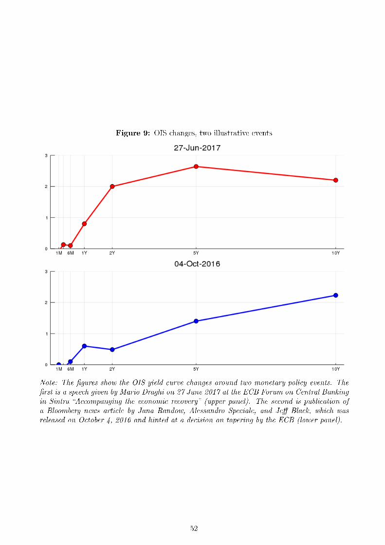
Figure 9: OIS changes, two illustrative events

Note: The �gures show the OIS yield curve changes around two monetary policy events. The�rst is a speech given by Mario Draghi on 27 June 2017 at the ECB Forum on Central Bankingin Sintra �Accompanying the economic recovery� (upper panel). The second is publication ofa Bloomberg news article by Jana Randow, Alessandro Speciale, and Je� Black, which wasreleased on October 4, 2016 and hinted at a decision on tapering by the ECB (lower panel).

52

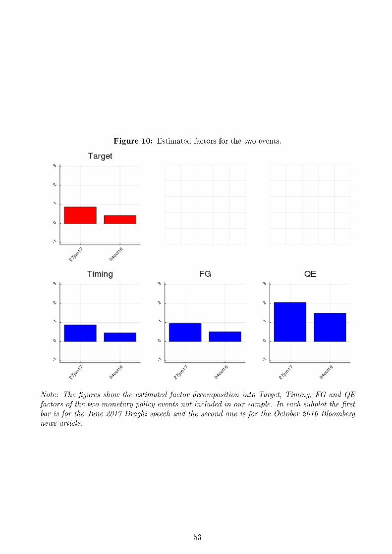
Figure 10: Estimated factors for the two events.

Note: The �gures show the estimated factor decomposition into Target, Timing, FG and QEfactors of the two monetary policy events not included in our sample. In each subplot the �rstbar is for the June 2017 Draghi speech and the second one is for the October 2016 Bloombergnews article.

53