Measuring District-Level Partisanship with Implications ... · nu m ber of congressional districts is ve ry difÞ cu lt, give n the data-gathering tech no logies an d resea rch bu

Measuring District-Level Partisanship withImplications for the Analysis of U.S. Elections*

Matthew S. Levendusky University of Pennsylvania

Jeremy C. Pope Brigham Young University

Simon D. Jackman Stanford University

Studies of American politics, particularly legislative politics, rely heavily on measures of the partisanship of a district.We develop a measurement model for this concept, estimating partisanship in the absence of election-specific, short-term factors, such as national-level swings specific to particular elections, incumbency advantage, and home-stateeffects in presidential elections. We estimate the measurement model using electoral returns and district-leveldemographic characteristics spanning five decades (1952–2000), letting us assess how the distribution of districtpartisanship has changed over time, in response to population movements and redistricting, particularly via thecreation of majority-minority districts. We validate the partisanship measure with an analysis of congressional roll-call data. The model is easily extended to incorporate other indicators of district partisanship, such as survey data.

Almost all empirical studies of congressionalelections rely on a measure of district parti-sanship, be they studies of incumbency ad-

vantage (e.g., Gelman and King 1990), challengereffects (e.g., Jacobson and Kernell 1983), redistricting(e.g., Cox and Katz 1999), regional differences inthe electorate, or national forces in elections (e.g.,Kawato 1987). These analyses share a common meth-odological strategy: estimating the effects of more orless transient factors (e.g., candidates and issues) onthe vote by statistically controlling for the partisan orideological disposition of a district. These studiesstand or fall on the quality of the measure of districtpartisanship. Consider a regression of district levelvote shares on variables of substantive interest and acontrol for district partisanship. If the district parti-sanship measure is measured with error, then notonly is the coefficient on district partisanship biased,but so too is the coefficient on any variable correlatedwith district partisanship, either directly or indirectly.Thus, an approach that better measures the under-lying concept—district partisanship—can improveestimation of all of those quantities and enhance

the validity of substantive conclusions. In this paperwe provide such a measure.

District Partisanship: Theory andMeasurement

Our approach rests upon decomposing voting behav-ior into long-term and short-term components, anapproach with a long and distinguished lineage inpolitical science, dating at least to Converse’s (1966)concept of the ‘‘normal vote.’’ The normal vote growsdirectly out of the Michigan team’s micromodel ofvoting behavior, in which party identification gener-ates stability in voting behavior, subject to election-specific responses to candidates and issues. The normalvote is the aggregate-level analog of enduring micro-level political loyalties and rests on decomposing voteshares into two components: a long-term, stablecomponent driven by party identification (the normalvote), and a short-term rate of defection generated bythe specifics of the campaign and the candidates

*We thank Chris Achen, Daniel Bergan, David Brady, Jay Goodliffe, John Jackson, Gary King, Keith Poole, Doug Rivers, HowardRosenthal, participants at the 2003 and 2005 Political Methodology Society Meetings and the Stanford Measurement Conference(August 2003) for useful comments. We also thank E. Scott Adler, Brandice Canes-Wrone, Joshua Clinton, John Cogan, Gary Jacobson,Stephen Ansolabehere, and Jim Snyder, and most of all, David Brady for generously providing us with access to their data.

The Journal of Politics, Vol. 70, No. 3, July 2008, Pp. 736–753 doi:10.1017/S0022381608080729

! 2008 Southern Political Science Association ISSN 0022-3816

736

(Converse 1966, 14).1 Our measure of district parti-sanship is analogous to Converse’s normal vote,except that Converse operationalized the conceptwith survey data on voting and party identification,whereas our measure relies on a mix of aggregateindicators (and in the extensions discussed in theonline appendix at www.journalofpolitics.org, surveydata). Like Converse, we seek to identify the more-or-less stable partisan force driving election outcomes.As such, our measure of district partisanship providesan estimate of how Democratic a given district wouldbe absent the impact of a given campaign (election-specific partisan swings, incumbency, etc.). That is,without any short-term forces, how Democratic orRepublican would a given district be?

We also want to be clear about what it is we arenot measuring. Measurement models use observedvariables to make inferences about latent variables.Consequently, the latent variable inherits its substan-tive content from the indicators available for analysisand our modeling assumptions. In our case, since werely heavily on district-level vote shares as indicators,the substantive content of our recovered latent traitcan not stray far from whatever substantive contentresides in vote shares (or the determinants of voteshares). Given that we have data on vote shares, butnot, say, survey data, we will resist claiming that wevalidly measure ‘‘district ideology.’’ Of course, to theextent that presidential and congressional voting isdriven by ideology, then our measure will haveideological content. For now, using only vote shares(as opposed to, say, survey data on individual prefer-ences), we take a conservative approach and interpretour measure as district partisanship rather than districtideology. However, in the online appendix, we aug-ment our model with survey measures of ideology todemonstrate one approach to validly estimating dis-trict ideology. Likewise, we will resist stating that ourmodel provides valid estimates of district preferences,such as the relative locations of each district’s median/mean voter. Our measurement model does not oper-ationalize a structural voting model that maps from

voter ideal points on a policy continuum to district-level vote shares. While it would no doubt be worth-while to investigate such a model (e.g., Snyder 2005),that endeavour is beyond our current scope.

Previous work has employed roughly three typesof measures for district partisanship: surveys, electionreturns, and demographic data. Each method hassignificant limitations.

Survey-based methods. Almost all survey-basedmethods suffer from a profound design challenge,sometimes referred to as the ‘‘Miller-Stokes problem.’’Miller and Stokes (1963) were interested in the extentto which members of Congress responded to districtopinion. But the data they had for any individualcongressional district was extremely sparse; their studyused a national probability sample that had an averageof only 13 respondents per congressional district (seeAchen 1978; Erikson 1978). And in general, generatingrepresentative samples of useful sizes from a usefulnumber of congressional districts is very difficult,given the data-gathering technologies and researchbudgets typically available to political scientists.2 Witha given budget constraint, researchers face an obvioustradeoff between surveying fewer respondents in moredistricts (sacrificing within-district precision for cross-district coverage) or surveying more respondents infewer districts (buying precision at the cost of cover-age); see Stoker and Bowers (2002) for an elaboration.In the face of limited research budgets either coverageor precision must suffer, and hence most attempts togenerate measures of partisanship (or preferences) spe-cific to congressional districts rely on aggregate data.3

Demographic Aggregates. Examples of thismeasurement strategy include Kalt and Zupan’s(1984) analysis of specific industries capturing mem-bers of Congress: in their analysis of Senate voting onstrip mining regulation, Kalt and Zupan took state-level data on membership in pro-environmentalinterest groups and the size of various coal producer

1The majority of work using the concept of a normal vote hasfollowed Converse’s initial approach and used survey data,examining rates of party voting within and across categories ofpartisan identifiers (e.g., Goldenberg and Traugott 1981; Petrocik1989). This approach has been rightly subject to criticism, on thegrounds that party identification is not exogenous, but respondsto the same short-term forces that shape vote decisions in anygiven election (e.g., Achen 1979). We stress that althoughConverse’s concept of a normal vote underlies our approach,our goal is to measure district partisanship (or the normal vote)at the level of congressional districts, and we do so with aggregatedata, with a set of controls that let us decompose vote shares intoshort-term and long-term components.

2Clinton (2006) is a rare exception, exploiting the unusualconfluence of two large studies of the American electorate in2000 (the Annenberg National Election Survey and a large panel ofonline respondents from Knowledge Networks) to yield estimatesof district ideology with an average of 232 respondents per district.

3Ardoin and Garand (2003) propose a novel application of surveydata to this problem: using the Wright, Erickson, and McIver(1985) state-level measures, they use the connection betweendemographic variables and this ideology measure to formdistrict-level estimates of constituent ideology for the 1980sand 1990s. While the method is an excellent application ofsurvey data, it is limited in that it can only generate results for the1980s and 1990s due to question wording changes. The methodwe present below, on the other hand, covers the entire post-warperiod and uses easily accessible data (demographic data from theU.S. census and electoral returns).

measuring district-level partisanship with implications 737

and consumer groups as indicative of economicinterests and preferences over regulation, inter alia.In a more general analysis, Peltzman (1984) used sixdemographic variables measured at the county levelto tap politically relevant, economic characteristics ofsenators’ constituencies.

A measure of district partisanship that reliedsolely on demographic characteristics of the districtsuffers from an obvious threat to validity. Demo-graphic attributes are generally considered antece-dents of partisanship, rather than indicators of it. So,while demographic characteristics may correlatehighly with one another and would appear tomeasure something about districts, there is no guar-antee that demographic characteristics alone wouldpermit us to locate congressional districts on apartisan continuum. That is, the use of demographicsalone may generate a measure of district partisanshipwith high reliability, but dubious concept validity.

Electoral Returns. Election returns are popularand easily accessed proxies for district partisanship.For instance, Canes-Wrone, Cogan, and Brady(2002), Ansolabehere, Snyder, and Stewart (2001),and Erickson and Wright (1980) all use district-levelpresidential election returns as a proxy for districtpartisanship in models of legislative politics. Thevirtue of this proxy is that it is based on constituentbehavior (vote choices) and is thus linked to thepartisan or ideological continuum that generallyunderlies electoral competition. Thus, a measure ofdistrict partisanship utilizing vote shares can beassumed to have high validity. But there are short-comings and trade-offs here as well. Presidential voteshares in any given election may be products of short-term forces; for instance, different issues are more orless salient in any given election, and particularcandidates are more or less popular. And over thelong-run, averaging a district’s presidential voteshares may well be a valid (i.e., unbiased) indicatorof district partisanship over the same period (e.g.,Ansolabehere, Snyder, and Stewart 2000), as theshort-term forces could plausibly cancel one anothergiven enough elections. But this is rather speculative.How much bias results from using the last two orthree presidential elections to estimate district parti-sanship? Moreover, shouldn’t researchers relying onpresidential vote confront the reality that they areusing a proxy for the underlying variable of interest?And even more fundamentally, researchers ought todeal with the fact that district partisanship can neverbe known with certainty. Like so many other varia-bles of interest to political science, district partisan-ship is not directly observable by researchers. Cast in

this light, we view election results as merely indica-tors of an unobserved variable of substantive interest.

The shortcomings of the approaches just sur-veyed suggests that we need a measurement strategyfor district partisanship that delivers the conceptvalidity provided by election returns, but that alsofilters out the impact of short-term factors. And as weshow below, this is precisely what our model does.We also note that not all district partisanshipmeasures fit into the categorization given above.Party registration data (Desposato and Petrocik2003), voting on down-ballot elections (e.g., Ansola-behere and Synder 2002) or propositions (e.g.,Gerber and Lewis 2004) and other factors may beused as proxies for a district’s partisanship. One ofthe useful features of our model is that these types ofpartially observed indicators can be easily added toany ensemble of indicators, consistent with thenotion that more information about the quantitybeing measured is better.

A Statistical Model for LatentDistrict Partisanship

We model district-level election outcomes as afunction of a more-or-less stable latent trait, specificto each congressional district. The latent trait isconsidered constant until redistricting intervenes;typically this happens once per decade. Electionoutcomes are also partially determined by election-specific short-term forces, generating vote shareseither greater or smaller than that we would expectgiven the district’s partisanship. These short-termforces include the presence of an incumbent or anexperienced challenger in congressional elections, andnational-level trends running in favor of one majorparty or presidential candidate.

It is possible to relax the assumption that eachdistrict’s latent trait remains unchanged over adecade. Generational replacement and other social-structural changes are continuous processes, and it isperhaps more realistic to consider the district-specificlatent trait as evolving over time. The chief difficultywith operationalizing a dynamic model of districtpartisanship is a lack of data: aside from electionoutcomes, we lack many time-varying covariates atthe district level. Variation in election outcomes onlysupplies so much information: it is extremely difficultto use a sequence of presidential and congressionalvote shares to recover estimates of both changingdistrict partisanship and the role of election-specificfactors (incumbency, presidential candidates, etc.).

738 matthew s. levendusky, jeremy c. pope, and simon d. jackman

Absent more time-varying, district-level data, restric-tive assumptions are another way to let districtpartisanship evolve over time. For instance, if weare willing to assume that there are no short-termforces (i.e., each election generates a faithful mappingfrom district partisanship to election outcomes) thenwe could obtain a new estimate of district partisan-ship at each election, but these assumptions seem toostrong. Therefore we treat district partisanship as aconstant but unknown attribute of a district, untilredistricting intervenes and/or decennial census pro-vides a new set of demographic covariates.

Our statistical model has two connected parts: onein which latent district partisanship appears as anunobserved left-hand-side variable, and the other inwhich latent district partisanship is a determinant ofvote shares. Let i 5 1, . . . ,n index districts, xi 2 R bethe latent partisanship of district i and zi be a k-by-1vector of demographic characteristics for district i.Both xi and zi are considered time-invariant: demo-graphic characteristics are measured just once each‘‘era’’ (in the decennial census) and (as discussedabove) we also treat district partisanship as fixed overthis period. Thus this part of the model is

xijziiid; N!z0ia; s

2" !1"

where a 2Rk is a set of parameters to be estimated,and s2 is an unknown variance. We impose theidentifying restriction that the latent xi have meanzero and variance one across districts; note that thisrestriction places an upper bound on s2.4 Theassumptions of normality and conditional independ-ence and homoskedasticity for xi given demographiccharacteristics zi are standard, if tacit, in measure-ment models.5

For the electoral data, we exploit the fact that ourdata have a panel structure—we have five Congres-sional elections and two or three Presidential elec-tions per district per decade. Given this structure, we

estimate the following model for congressionalelections:

y#ijjxiiid; N!mij; n

2j " !2"

where

mij5 gj1 $ gj2xi $ controls !3"

and where i indexes districts and j indexes Houseelections; y#ij5 ln yij

1%yij

! "and yij 2 (0, 1) is the

proportion of the two-party vote for the DemocraticHouse candidate in district i at election j; n2j is thedisturbance variance; gj1 is an unknown fixed effectfor each election, tapping the extent to which na-tional level factors (e.g., macroeconomic conditionsor a national scandal) drive outcomes in con-gressional election j; gj2 is an unknown parametertapping the extent to which district partisanship xidetermine vote shares; and we also include indicatorstapping incumbency offsets (whether a Democraticincumbent is running for reelection, and similarly forRepublican incumbents) and challenger quality(whether the Democratic or Republican challengerhas held elected office). We also interact the indica-tors for Democratic and Republican incumbents witha dummy variable for Southern districts, thus makingour estimates of incumbency offsets conditional onwhether the district is an a southern or nonsouthernstate (we make no distinction between open seats insouthern and nonsouthern states). Note that we termthe quantities we estimate ‘‘incumbency offsets’’rather than ‘‘incumbency advantage.’’ We adopt thisrhetorical convention to avoid interpreting theseparameters as the causal effects of incumbencyadvantage because of the potential for post-treatmentbias in our model.6

The model for presidential elections is similar,but with different predictors, and has the log-odds ofthe Democratic share of the two-party presidentialvote in district i in presidential election k as thedependent variable:

y#ikjxiiid; N!mik; n

2k" !4"

where

mik 5 bk1 $ bk2xi $ controls !5"

4Our assumption that xi is unidimensional is supported by boththeory and the data. From a theoretical perspective, districtpartisanship (like normal vote) runs from a purely Republicandistrict to a purely Democratic one, with each district in betweenthese two types. Empirically, principal components analysis of thedata overwhelmingly supports a unidimensional construct, seethe appendix for further details.

5Moreover, since xi is unobserved, it is not straightforward tocheck these assumptions. The conditional independence assump-tion could be replaced with some kind of spatial dependencestructure, although we are reasonably confident that the set ofdemographic predictors zi assembled for analysis does generateconditional independence among the xi; we would be lessconfident in this assertion if zi was a less exhaustive set ofindicators.

6Because district partisanship is fixed over a decade, the (say)1996 vote returns influence the estimate of district partisanship,which in turn might influence the 1992 incumbency offsetparameter, so what we provide is not an estimate of incumbencyadvantage as conventionally understood. Rather, we are trying toremove the short-term effect of incumbency so we can estimatethe underlying latent partisanship more accurately.


and where bk1 is an unknown fixed effect forpresidential election k; bk2 is defined similarly togj2, above; the controls tap home state offsets, i.e.,dummy variables for whether the Democratic andRepublican presidential and vice-presidential candi-dates hail from the state in which district i is located.

Finally, a brief word on redistricting is alsowarranted. Most redistricting takes place in the wakeof the decennial census, in time for the election in the‘‘2’’ years (1982, 1992, etc.). But a considerableamount of redistricting occurs at other times (e.g.,the Texas redistricting prior to the 2004 election).This presents a problem: districts sometimes changemid-cycle, so (for example) FL-2 in 1992 is not thesame district as FL-2 in 2000. To resolve thisproblem, we treat the district prior to redistrictingas one district, and the district post-redistricting as aseparate district, each with its own distinct latenttrait.7 If the redistricting occurred prior to the (say)1996 election, then the post-redistricting district ismissing elections from 1992 and 1994, and the pre-redistricting district is missing electoral returns from1996 forward.

A stylized, graphical summary of the modelappears in Figure 1, using the convention thatunobserved quantities appear in circles, and observedquantities appear in rectangles. Election outcomes areakin to multiple indicators of district partisanship, xi,and are treated as conditionally independent of eachother given xi and other predictors. In particular,note that we (1) augment the models for the variouspresidential and congressional election outcomes(equations 2 through 5) with politically relevantcovariates (e.g., indicators for incumbency, chal-lenger quality, region, home-state effects, and elec-tion-specific fixed effects) and (2) exploit theinformation in census aggregates about district par-tisanship via equation (1). As Figure 1 demonstrates,demographic characteristics give rise to district par-tisanship, and then that district partisanship is usedto model the election outcomes.8

Bayesian Estimation and Inference

Our model is a structural equations model (SEM), asthey are known in psychometrics. While manypolitical scientists are most familiar with estimationof these models using covariance structure methods—via software such as LISREL, AMOS, EQS—we adopta Bayesian approach for estimation and inference.

Advantages of a Bayesian Approach

First, a primary goal of our analysis is measurement:i.e., to produce estimates of district partisanship,along with rigorous assessments of uncertainty (e.g.,standard deviations, confidence intervals), since ab-sent uncertainty assessments, the point estimates ofdistrict partisanship can not be meaningfully com-pared. We also require uncertainty assessments whenwe use our measure in subsequent analysis. Uncer-tainty over levels of district partisanship ought topropagate into assessments of the effects of districtpartisanship when it appears as a predictor ofpolitical outcomes (e.g., in models of election out-comes, legislative behavior, and the like).

Most analysis of covariance structure approachestreat the latent variables xi as nuisance parameters,and, at best, will produce point estimates of these

FIGURE 1 Stylized, Graphical Representation ofModel for the 1990s. Districtpartisanship is the latent variabledenoted x in the graph.

7To determine whether or not a district has been redistricted, weuse Gary Jacobson’s Congressional elections dataset and ScottAdler’s district demographic dataset; we treat a district as havingbeen redistricted when these data sources concur.

8Another interpretation of the model is as a hierarchical ormultilevel model (e.g., Hox 2002; Skrondal and Rabe-Hesketh2004); i.e., the latent district partisanship parameters, xi, aretreated here as similar to ‘‘random effects,’’ but with a ‘‘level 2’’regression model (equation 1) exploiting information aboutlatent district partisanship in the time-invariant census aggre-gates, zi.


quantities conditional on estimates of the factorstructure; the resulting latent trait estimates areknown as ‘‘factor scores’’ in the factor analysisliterature (e.g., Mardia, Kent, and Bibby 1979).Producing uncertainty estimates for factor scores inan analysis of covariance structure framework posesboth statistical and computational challenges and isseldom done (cf. Joreskog 2000). In our analysis,levels of district-level partisanship are of primaryinterest, and relegating them to the status of nuisanceparameters is problematic (for a similar point, seeAldrich and McKelvey 1977).

However, working in a Bayesian framework,latent district partisanship is treated no differentlyfrom any other model parameter. We compute thejoint posterior density of all model parameters,recognizing the fact that in measurement models itis almost always the case that uncertainty in measure-ment parameters generates uncertainty in the latenttraits, and vice-versa; for a recent elaboration of thispoint, see Dunson, Palomo, and Bollen (2007). Ofcourse, working with the joint posterior density of allparameters comes at some computational cost: withone latent district partisanship parameter for eachcongressional district and numerous other parame-ters to estimate, there are many parameters in ourmodel, and the resulting posterior density is highdimensional. Happily, one of the benefits of theBayesian approach is that we can exploit Markovchain Monte Carlo (MCMC) algorithms that visitlocations in the parameter space with relative fre-quency proportional to the posterior probability ofeach location. That is, let run long enough, eachiteration of the MCMC algorithm produces a samplefrom the joint posterior density. We summarize thesesamples so as to make inferences about the param-eters. See Jackman (2000) for a review; further detailsappear in the appendix.

Once we possess arbitrarily many samples fromthe posterior density, inference for the latent traits isstraightforward. For example, we can assign proba-bilities to politically relevant statements such as‘‘district i is more Republican than district j,’’ ‘‘dis-trict i is the most Republican district in the country,’’‘‘district i is the most Democratic district held by aRepublican,’’ or ‘‘district i is the median district,’’simply by noting the proportion of MCMC iterates inwhich a particular assertion about the latent traits istrue. This is a remarkably simple way to performinference for the latent traits, relative to the work onewould have to do to obtain such inferences withthe output of factor analytic/covariance-structureapproaches.

Perhaps the chief advantages of the Bayesianapproach lie in its flexibility and extensibility. Takethe case of missing data arising from uncontestedseats. This is a significant issue in our data. In everydecade we analyze, at least a quarter of the districtshave at least one uncontested election, and in the1980s the corresponding figure is 45%. One solutionwould be to drop these particular elections from theanalysis, but this could lead to significant bias (recallwe would be dropping more than a quarter of thesample). This data is not missing at random, sostandard imputation techniques are inappropriatehere. Indeed, the fact that an incumbent was reelectedunopposed is informative about underlying districtpartisanship. We model uncontested elections ascensored data, an approach used by Katz and King(1999) in their analysis of British House of Commonselection returns. That is, if a Democratic incumbentsuccessfully runs unopposed then we model theunobsered vote share via equation (2), subject tothe constraint that the two-party Democratic voteshare is greater than 50% (i.e., that yij . .5 5y*ij . 0) ensuring that uncontestedness is contribu-ting some information about district partisanship.This constraint is trivial to implement with our latentvariable model. Imposing this (or any other non-standard) restriction in an analysis of covariancemodel is extremely difficult, if not impossible. Inan analysis of covariance model, to the best of ourknowledge, one would have to settle for either list-wisedeletion or imputation based on missing at randomtechniques, both of which are inappropriate here.9

Priors Densities over Parameters

In any Bayesian analysis it is incumbent on theresearcher to report what prior densities are em-ployed. Recall that we impose the identifying restric-tion that the latent xi have mean zero and varianceone. With this restriction the model parameters areidentified and we use vague priors, letting the datadominate inferences for these parameters: i.e., apriori we specify independent N(0, 102) priors forthe regression parameters g and b and vague inverse-Gamma priors for the variance parameters. Withthese normal and inverse-Gamma priors, and thenormal distributions assumed for the hierarchicalstructure over the latent district partisanship

9As an additional robustness check, we have also reestimated ourmodel using both an unconstrained imputation technique (e.g.,imputations without the constraint) and treating election out-comes in uncontested seats as missing at random. The substan-tive results generally remain similar.


(equation 1) and the observed vote shares (equations2 and 4), the resulting posterior densities for allmodel parameters are in the same family as theirprior (normals and inverse-Gammas), ensuring thatthe computation for this problem is rather simple (acase of conjugate Bayesian analysis); see the appendixfor further details.

Results: Measuring DistrictPartisanship

Each congressional district’s latent partisanship ap-pears in our model as a parameter to be estimated, xi.Via our Bayesian approach and our use of a Markovchain Monte Carlo algorithm, we obtain manysamples from the joint posterior density of all thexi. In turn, we induce a posterior density over theorder statistics of the xi, letting us assess the extent towhich we can a distinguish districts from oneanother. Graphical summaries appear in Figure 2.

The top panel of Figure 2 displays point estimatesof each district’s latent partisanship (the mean of themarginal posterior density for each xi) for the 1990sdata; the thin gray lines are pointwise 95% credibleintervals, computed as the 2.5th and 97.5th quantilesfrom 1,000 Gibbs samples thinned from 250,000samples. Similar graphical summaries can be con-structed for earlier years; space constraints restrictthis detailed examination to the most recent decadein our analysis, the 1990s. The actual numbers in thetop panel attaching to the estimate are arbitrary;recall that the xi are only defined up to scale andlocation, and the identifying restriction we employ isthat the xi have mean zero and standard deviationone. However, relative comparisons are meaningful,as is an assessment of the uncertainty attaching toeach xi relative to the between-district variation in thexi, and the shape of the distribution of the xi.

By construction, between-district variation inlatent district partisanship has a standard deviationof 1.0 while the average posterior standard deviationfor the district partisanship estimates in the 1990sdata is .10; that is, as the top panel of Figure 2suggests, differences across districts are generally largerelative to the uncertainty that attaches to eachdistrict’s xi. On the other hand, the bottom panel ofFigure 2 suggests the limits with which we can makefine distinctions among districts. For moderate dis-tricts, the 95% credible interval on each district’s rankcovers about 90 places, or about 20% of the districtsin the data. Some insight into the consequences of

this uncertainty comes from comparing two relativelymoderate districts, say, the districts at approximatelythe 45th and 55th percentile of the distribution ofthe xi (e.g., MI-7 and PA-4), respectively. Our bestguesses (posterior means) for these districts’ latentpartisanship are -.26 and -.09, and the probabilitythat PA-4 is more Democratic than MI-7 is .91. Finerdistinctions in the middle of the distribution of latentdistrict partisanship are made with less certainty, andwill fall short of traditional standards used in hy-pothesis testing. On the other hand, in the tails of thedistribution, fine distinctions can be made morereadily: for instance, the probability that a districtat the 1st percentile (e.g., AL-6) is more Republicanthan a district at the 3rd percentile (e.g., KS-1) isgreater than .99.

Additionally, Figure 2 shows the effect of redis-tricting and uncontestedness: both increase our un-certainty of the district’s partisanship. Notice that

FIGURE 2 Latent District Partisanship, 1990s:Pointwise Means and 95% CredibleIntervals (top panel), Order Statisticsand 95% Credible Intervals (bottompanel).


some districts have much wider credible intervalsthan others, reflecting the increased uncertaintystemming from having fewer elections contributingdata for those districts.

The distribution of latent district partisanshiphas a pronounced right-hand skew. The most Dem-ocratic districts are roughly four standard deviationsaway from the mean district (set to zero, by con-struction). On the other hand, the most Republicandistricts in the country are just two standard devia-tions away from the mean. Quite simply, the mostDemocratic districts in our data exhibit more con-sistent and more heavily Democratic voting patternsthan the Republican districts exhibit extreme pro-Republican voting patterns. For instance, in the 10most Democratic districts, Clinton averaged 89%of the two-party vote share in 1992 and 1996; inthe 10 most Republican districts, Clinton averaged30%, while in the remaining districts, Clinton aver-aged 54%.

Figure 3 shows the densities (smoothed histo-grams) of our district partisanship estimates in eachof the five decades we study. In each decade districtpartisanship is normalized to have a mean of zeroand unit variance across districts, so these graphs arenot informative about any long-term trends inaverage levels of district partisanship (e.g., say, ifthe country, on average, was trending in a particularpartisan direction), or increases in the dispersion ofdistrict partisanship (e.g., as might arise if redistrict-

ing was a source of partisan polarization, via thecreation of lop-sided districts etc.). Nonetheless, thedensities in Figure 3 do illustrate the way that districtpartisanship consistently has a skewed distribution,and ways in which that skew has changed over time,reflecting both population movements and redistrict-ing. Specifically, in every decade we examine, thereare a relatively small number of extremely Democraticdistricts, without an offsetting set of extremelyRepublican districts. This Democratic skew in thedistribution of district partisanship is at its leastpronounced in the first decade we analyze, the1950s, and reaches its peak in the 1980s, where IL-1(located on Chicago’s south side) lies six standarddeviations away from the average district.

More generally, the overwhelmingly Democraticdistricts in recent decades are almost all majority-minority districts. Unsurprisingly, and as we elabo-rate below, the racial composition of a district is apowerful determinant of its partisanship (see Table 1).For instance, the most Democratic district in ouranalysis of the 1990s is NY-16 (centered on the SouthBronx in New York City), whose population in the1990 Census was reported as 59% Hispanic originand 43% black (these categories are not mutuallyexclusive); Barone and Ujifusa (1995, 946) state that‘‘[p]olitically . . . [NY-16] . . . is quite possibly themost heavily Democratic district in the country.’’The adjoining seat, NY-15 (centered in Harlem), isthe second most Democratic seat in our analysis of

FIGURE 3 Density plots of district partisanship estimates (means of marginal posterior densities), bydecade; higher values of district partisanship indicate more Democratic districts. Recall thatfor each decade, the district partisanship estimates are recovered subject to the identifyingrestriction that they have mean zero and unit variance across districts.


the 1990s; it has been held by Charlie Rangel since1970 and was 47% black and 45% Hispanic origin inthe 1990 Census. NY-10 and NY-11, both in Brooklyn,are the third and fourth most Democratic seats inour analysis, with black populations of 60% and75%, respectively. Districts in central Philadelphia(PA-2, 62% black), central Detroit (MI-15, 70%black; MI-14, 69% black), the south side of Chicago(IL-1, 70% black; IL-2, 68% black), and SouthCentral Los Angeles (CA-35, 43% black and 42%Hispanic origin) round out the 10 most Democraticdistricts in the 1990s. The correlation between thepercentage of the district’s population that is AfricanAmerican and our measure of district partisanship is.60 in the 1990s.

Validating the District PartisanshipMeasure

Figure 4 shows a scatterplot of the recovered latenttrait and its indicators (presidential and congres-sional vote shares) for the 1990s; similar plots forother decades are provided in the online appendix.The relationship between the vote shares and thelatent trait is fairly strong, given that our model treatsvote shares as an indicator of the latent districtpartisanship. The nonlinearities follow from usinglog-odds transformations of the vote shares as in-dicators of latent district partisanship (equations 2and 4). Outliers are generally more prevalent in thecongressional elections scatterplots, resulting fromthe fact that congressional elections outcomes aremodeled not only as a function of latent districtpartisanship, but also with offsets for incumbency,challenger quality, and region (south/nonsouth).

A more realistic assessment of both the validityand usefulness of our measure of district partisanshipcomes from seeing how well it predicts politicaloutcomes not in our model, but still plausiblyrelated to district partisanship. The criterion vari-able we use is legislative preferences, as revealed viaroll-call voting. Figure 5 presents a scatterplot oflegislative preferences (‘‘ideal points’’) against ourmeasure of district partisanship for the 1990s (again,see the appendix for similar displays from otherdecades). The legislative ideal points are generatedwith a one-dimensional spatial voting model fit toall nonunanimous roll calls cast in the 107th U.S.House of Representatives (2001–2002), using themodel and estimation procedures described inClinton, Jackman, and Rivers (2004). Where adistrict was represented by more than one legislatorover the course of the 107th Congress (e.g., due toT

ABLE1

Posterior

Summaries,RelationshipsBetweenDem

ographic

Characteristicsan

dLatentDistrictPartisanship.Cellentriesareposterior

means;95%

credible

intervalsshow

nin

brackets.Medianincomeismedianfamilyincome;pop

ulation

density

ispop

ulation

per

mile2;

South

isdefined

asthe11

states

oftheform

erconfederacy.

SeeAdler(2003)

foradditional

details.

1952-1960

1962-1970

1972-1980

1982-1990

1992-2000

Intercept

7.94

[3.96,

11.87]

27.13[20.17,35.58]

31.16[21.67,41.94]

22.88[17.90,29.88]

16.94[13.17,21.22]

Log

Proportion

Aged65+

20.71

[21.07,20.34]

20.79

[21.06,2

0.53]

20.40

[20.67,20.14]

0.038[2

0.18,0.26]

0.47

[0.28,

0.65]

Log

Proportion

BlueCollar

20.24

[20.58,0.11]

0.33

[20.088,

0.74]

0.24

[20.085,

0.57]

20.16

[20.39,0.077]

20.071[2

0.26,0.12]

Log

Proportion

ForeignBorn

20.05

[20.16,0.05]

0.33

[0.22,

0.44]

0.11

[0.0069,

0.21]

0.08

[20.0075,0.17]

0.20

[0.13,

0.28]

Log

MedianIncome

21.18

[21.60,20.72]

22.62

[23.14,22.11]

22.70

[23.27,22.12]

21.88

[22.23,21.52]

21.05

[21.40,20.68]

Log

Pop

ulation

Density

0.14

[0.087,0.20]

0.17

[0.13,

0.21]

0.27

[0.22,

0.32]

0.19

[0.14,

0.23]

0.22

[0.18,

0.26]

Log

Proportion

Unem

ployed

0.34

[0.10,

0.58]

0.57

[0.28,

0.86]

0.48

[0.19,

0.75]

0.60

[0.37,

0.85]

0.85

[0.59,

1.14]

Log

Proportion

Black

0.12

[0.045,0.20]

0.12

[0.058,0.18]

0.089[0.022,0.16]

0.066[0.0088,

0.12]

0.094[0.035,0.15]

South

(dummy)

0.49

[0.0095,

0.98]

20.36

[20.87,0.11]

20.14

[20.61,0.28]

20.27

[20.62,0.074]

0.14

[20.15,0.43]

Log

Proportion

Black

xSouth

0.23

[0.043,0.42]

0.12

[20.074,

0.32]

0.0088

[20.17,0.18]

0.14

[0.0083,

0.27]

0.30

[0.19,

0.40]

Majority-Minority

22

22.05

[1.61,

2.47]

0.93

[0.56,

1.31]

sx

0.75

[0.69,

0.80]

0.70

[0.65,

0.75]

0.69

[0.64,

0.73]

0.56

[0.53,

0.61]

0.50

[0.47,

0.54]

r2 x0.44

[0.36,

0.52]

0.51

[0.43,

0.58]

0.53

[0.46,

0.59]

0.68

[0.63,

0.72]

0.75

[0.71,

0.78]


deaths and retirements), we display the ideal point ofthe legislator with the lengthier voting history. Bothlegislative ideal points and district partisanship areestimated with uncertainty, indicated with the verti-cal and horizontal lines covering 95% credibleintervals, respectively.

In general, there is a strong relationship betweendistrict partisanship and legislative ideal points; thecorrelation between the two sets of point estimates is0.73. The within-party correlations are also moderateto large: 0.47 among Republicans, and 0.52 amongDemocrats. We would not expect a perfect or evennear-perfect relationship between district partisan-ship and a measure of legislators’ preferences, sincethere are many plausible sources of influence on roll-call voting other than district partisanship, withparty-specific whipping perhaps the most prominent.Indeed, perhaps the most noteworthy feature ofFigure 5 is the separation of legislators’ ideal pointsby party; there is almost no partisan overlap in theestimated ideal points, while there is considerableoverlap in estimates of district partisanship across thetwo parties. No scholar of contemporary Americanpolitics would be surprised by this finding, although alively debate continues as to the sources of polar-ization within the Congress (e.g., McCarty, Poole,

and Rosenthal 2003). The pattern in Figure 5 isconsistent with a party-pressure hypothesis (e.g.,Synder and Groseclose 2000), or a more generalprocess of polarization among political elites, show-ing that there is virtually no overlap between the idealpoints by party, while there is considerable overlapin our estimates of district partisanship by party-of-representative. Put differently, there is muchmore partisan polarization in the roll-call votingthan in the corresponding estimates of districtpartisanship.

Further, suppose we break the distribution ofdistrict partisanship at its mean value of zero, labelingdistricts to the left of this point ‘‘Republican’’districts and districts to the right as ‘‘Democratic.’’Figure 5 reveals that there are 28 Democrats and sixRepublicans (13% and 3% of their respective caucu-ses) who represent districts that, by this criterion,should be represented by the other party. What canwe say about these districts? First, all but two of thesedistricts were represented by incumbents in the 107thCongress, many of them long-time incumbents.While most are still serving in Congress, nine ofthese 31 incumbents had been defeated by 2007, andnearly all of these defeated members had their lossattributed to their fit with the district by sources like

FIGURE 4 Vote Shares plotted against Latent District Partisanship, 1990s. Presidential election outcomesare modeled as a function of the latent trait plus intercept shifts for home-state effects.Similarly, the model for congressional election outcomes includes intercept shifts forincumbency, region and challenger quality.


the Almanac of American Politics (Barone Cohen2006; henceforth, AAP). And of the members stillserving, when they retire, the seat is likely to changepartisan hands. Take the case of Gene Taylor (D-MS):the AAP argues that if he were to retire, ‘‘Republicanswould have an excellent chance to capture this seat’’(AAP, 957). Indeed, of the members who have retired(a number of them were strategic retirements promp-ted by redistricting), in all but one case party controlof the seat flipped (the exception is Ted Stricklandwho retired to become governor of Ohio in 2006 andwas replaced by Democrat Charles Wilson; undoubt-edly the corruption scandal in the Ohio RepublicanParty played a role). Furthermore, nearly all of thesemembers are described as being political moderatesand mavericks out of step with their national partiesand more in line with their districts. In fact, 80% ofthe members with mismatched seats are described bythe AAP as ‘‘moderate,’’ ‘‘centrist,’’ ‘‘conservativeDemocrat,’’ ‘‘straddles both parties,’’ and so forth.Indeed, Ralph Hall, one of the Democrats represent-ing a Republican district, switched parties in 2004. Ofthe handful of members described as more typicalpartisans, nearly all of them are described by the AAP

as focusing on the ‘‘grassroots’’ or other issuesimportant to their district, suggesting that they winby promoting service to the district. Taken as awhole, this analysis suggests even more validity forour measure of district partisanship.

Since our main purpose is to measure and modeldistrict partisanship, we defer a more detailed anal-ysis of representation or polarization for another day;a complete list of ‘‘mismatched’’ members of Con-gress and their districts appears in the online appen-dix. For now we simply note that the the relationshipbetween our measure of district partisanship andelection returns is very strong (particularly in the1990s) and that the correlation between districtpartisanship and estimated legislator ideal points isconsistent with our general expectations. This notonly bolsters our confidence in the measure, butdemonstrates its usefulness for analyzing congres-sional politics.

Social-Structural Correlates of DistrictPartisanship

Table 1 presents parameter estimates of the demo-graphic component of the model (equation 1), wherelatent district partisanship is modeled as a function ofthese census aggregates. Of the many demographicvariables aggregated to the level of congressional districtsin the census, which ones are more politically relevantthan others? A long line of research with its roots inpolitical sociology suggests that indicators of social classought to be relevant in this context: these includemedian income or the composition of the workforce(e.g., unemployment rates, percent blue-collar, percentunionized). In addition, studies of committee assign-ments have focused on the role that particular demo-graphic characteristics play in shaping the behavior ofmembers of Congress. These studies supply predictionsabout how we might expect constituent partisanshipand demographic characteristics to be related; a usefulsummary appears in Adler and Lapinski’s (1997) listingof politically relevant district characteristics in theirstudy of demand for policy outputs from Congress.10

For the most part, the relationships we findbetween district partisanship and demographic charac-teristics contain few surprises, as presented in Table 1.First, and as discussed previously, districts with highproportions of African Americans are consistentlyamong the most Democratic districts. Over the fivedecades in our analysis, the coefficient on the log of

FIGURE 5 Legislative Preferences (legislators’ideal points) and latent districtpartisanship, 107th House. Verticaland horizontal lines indicate 95%credible intervals for legislativepreferences and district partisanship,respectively. The dotted vertical andhorizontal lines show the mean of therespective measures.

10Moreover, the demographic variables we use come from Adler’s(2003) dataset on Congressional district demographics.


the proportion of African Americans in the popula-tion (outside of the South) is always unambiguouslypositive, and averages about .10. In each decade, thedistribution of African Americans throughout con-gressional districts is skewed to the right: i.e., themedian African American proportion is consistentlyaround .10, but attains a maximum of .92 in the1980s (in IL-1), and .88 in the 1970s and 1960s, .74 inthe 1990s (in NY-11), and .69 in the 1950s (in MS-3),with an average 95th percentile of .42. Thus, in the1990s, in a non-Southern district, an increase in theproportion of the African American population fromthe mean level of .13 to .57 (the 95th percentile) isassociated with an increase of district partisanship ofapproximately 15% of a standard deviaton, net ofother factors. Additionally, the coefficient for major-ity-minority districts is large and statistically signifi-cant, indicating the even controlling for the fact thatmajority-minority districts contain a high percentageof African Americans, such districts are even moreDemocratic.

Other variables that are also consistently andstrongly associated with district partisanship aremedian income and population density. Richer dis-tricts (as measured by the district’s median per capitaincome) are consistently less Democratic than poorerdistricts. Our parameter estimates imply that net ofother factors, movement from the 5th to the 95thpercentile on income is associated with anywherefrom a standard deviation’s worth of change indistrict partisanship (e.g., 1950s and 1990s), to 2.1standard deviations of change in district partisanshipin the 1960s. Population density displays tremendousvariation in any given decade; movement from the5th to the 95th percentile on this variable is asso-ciated with shifting latent district partisanship astandard deviation (in a Democratic direction) inthe 1960s, but up to a two standard deviation shift inthe 1970s. Overall, the main result we stress from thissection is the strong and sensible relationship be-tween the demographics and our district partisanshipmeasure.

Congressional Elections

Estimates of the congressional elections models ap-pear in Tables 2 and 3. The models fit reasonablywell, with the r-squared values for the 25 equationsranging from a low of .65 in 1954 to a high of .90 in2000. The parameters tapping the effects of districtpartisanship range from a low of .26 in 1972 to .62 in

1956. Recent House elections, say, 1994–2000, havebeen characterized by (a) reasonably good model fitand (b) relatively high discrimination with respect tothe latent partisanship measure.

The estimates for the incumbency offset param-eters are of some substantive interest. Since our de-pendent variable in the vote equations is the log-oddsratio of vote shares, we implicitly have a nonlinearmodel in vote shares themselves; to simplify the assess-ment of the model’s marginal effects, we assess allmarginal effects conditional on vote shares being at50%, corresponding to districts that are otherwiseevenly split between Democrats and Republicans (notethat the 50-50 vote split is also the steepest part of thelogistic CDF, where marginal effects on votes taketheir maximum possible value). In addition, our con-gressional elections model includes terms for challengerquality (i.e., a dummy variable coded 1 if the challengerhas previously held elected office and 0 otherwise).

Incumbency offsets are estimated separately forNorthern and Southern states and also for Demo-cratic and Republican incumbents. The regionalvariation in the magnitude of the incumbency offsetsis perhaps the most striking feature of this part of theresults. For the 1950s, we estimate massive incum-bency offsets for Democratic incumbents in theSouth, worth anywhere from 10 to 20 percentagepoints of vote share in an otherwise evenly splitdistrict. Incumbency offsets for Northern Democratsand all Republicans in the 1950s are much smaller; infact, for Southern Republicans prior to the 1970s(when there are relatively few Southern Republicanincumbents in the House), our estimates of incum-bency offsets are indistinguishable from zero atconventional levels of statistical significance. In gen-eral, there is no systematic pattern of incumbencyoffsets being larger for one party than the other.11

There is some regional asymmetry, particularly onthe Democratic side, although this is concentratedprimarily in the early part of our study. Although westress we are estimating a different quantity ofinterest, our results closely parallel the larger liter-ature on the incumbency advantage, which finds asubstantial increase in the incumbency advantage inthe 1960s and 1970s, followed by modest decline inthe late 1980s and 1990s.12

11Evidence of a partisan asymmetry would be when the 95%highest posterior density interval on the sum of the Democraticincumbency offset and the (negatively signed) Republican in-cumbency offset does not overlap zero.

12For example, see Alford and Brady (1993), Gelman and King(1990), and Ansolabehere, Snyder, and Stewart (2001).


TABLE 2 Posterior Summaries, Congressional Elections Model, 1952-1974. Cell entries are posterior means, 95% credible intervals in brackets. In allyears, the dependent variable is the log-odds of the Democratic proportion of the two-party vote in contested House races. See equation 2.Challenger quality data is not available in all years.

Year InterceptDistrict

PartisanshipDemocraticIncumbency

RepublicanIncumbency

South x DemIncumbency

1952 0.053 [-0.031, 0.14] 0.50 [0.45, 0.55] 0.077 [-0.043, 0.19] 20.22 [20.32, 20.11] 0.95 [0.80, 1 09]1954 0.65 [0.47, 0.83] 0.58 [0.50, 0.67] 20.37 [20.59, 20.15] 20.58 [20.78, 20.37] 0.99 [0.76, 1.19]1956 0.31 [0.11, 0.53] 0.62 [0.54, 0.71] 20.22 [20.48, 0.029] 20.29 [20.51, 20.052] 1.17 [0.95, 1.40]1958 0.27 [0.18, 0.36] 0.37 [0.31, 0.42] 0.38 [0.26, 0.51] 20.28 [20.39, 20.17] 0.87 [0.70, 1.04]1960 0.20 [0.053, 0.33] 0.46 [0.39, 0.52] 0.19 [0.036, 0.37] 20.23 [20.40, 20.066] 0.73 [0.58, 0.89]1962 0.11 [0.038, 0.19] 0.32 [0.28, 0.36] 0.25 [0.15, 0.34] 20.40 [20.49, 20.30] 0.48 [0.36, 0.60]1964 0.34 [0.25, 0.43] 0.33 [0.29, 0.38] 0.30 [0.19, 0.40] 20.40 [20.51, 20.29] 0.10 [20.012, 0.21]1966 0.061 [20.028, 0.15] 0.36 [0.33, 0.40] 0.28 [0.17, 0.39] 20.57 [20.67, 20.45] 0.32 [0.21, 0.43]1968 0.22 [0.12, 0.32] 0.40 [0.36, 0.45] 0.15 [0.017, 0.28] 20.67 [20.78, 20.55] 0.46 [0.33, 0.59]1970 0.10 [0.0016, 0.20] 0.37 [0.32, 0.42] 0.51 [0.39, 0.64] 20.40 [20.51, 20.27] 0.38 [0.24, 0.53]1972 0.08 [20.0039, 0.17] 0.26 [0.22, 0.30] 0.59 [0.47, 0.70] 20.61 [20.73, 20.49] 0.015 [20.13, 0.15]1974 0.40 [0.29, 0.51] 0.32 [0.27, 0.37] 0.43 [0.31, 0.57] 20.55 [20.69, 20.41] 0.12 [20.023, 0.26]

YearSouth x RepubIncumbency

Dem ChallengerQuality

Rep ChallengerQuality nj r2

1952 0.023 [20.46, 0.47] - - 0.32 [0.29, 0.35] 0.81 [0.77, 0.84]1954 0.06 [20.36, 0.50] - - 0.52 [0.48, 0.57] 0.65 [0.59, 0.70]1956 20.022 [20.47, 0.41] 0.023 [20.16, 0.20] 0.12 [20.11, 0.39] 0.55 [0.50, 0.59] 0.65 [0.59, 0.71]1958 20.021 [20.26, 0.22] 0.13 [0.032, 0.23] 20.13 [20.26, 0.0068] 0.29 [0.27, 0.32] 0.80 [0.77, 0.84]1960 20.12 [20.48, 0.23] 0.031 [20.13, 0.18] 20.075 [20.21, 0.07] 0.40 [0.37, 0.43] 0.73 [0.68, 0.76]1962 0.15 [20.14, 0.40] 2 2 0.29 [0.26, 0.32] 0.79 [0.75, 0.83]1964 0.076 [20.13, 0.28] 0.091 [20.0087, 0.19] 20.13 [20.25, 20.010] 0.30 [0.27, 0.32] 0.78 [0.74, 0.81]1966 0.15 [20.027, 0.31] 0.044 [20.062, 0.15] 20.19 [20.28, 20.11] 0.23 [0.21, 0.26] 0.88 [0.85, 0.90]1968 0.082 [20.083, 0.24] 0.15 [0.047, 0.26] 20.10 [20.21, 0.012] 0.30 [0.27, 0.33] 0.85 [0.82, 0.87]1970 0.014 [20.14, 0.18] 0.10 [20.017, 0.22] 20.11 [20.23, 0.012] 0.31 [0.29, 0.34] 0.83 [0.80, 0.86]1972 20.26 [20.43, 20.099] 0.20 [0.059, 0.33] 20.21 [20.33, 20.091] 0.35 [0.33, 0.38] 0.78 [0.75, 0.81]1974 20.18 [20.32, 20.037] 0.18 [0.06, 0.29] 20.09 [20.27, 0.098] 0.37 [0.34, 0.40] 0.76 [0.72, 0.79]

748matth

ews.lev

endusky,jerem

yc.

pope,

andsim

ond.jack

man

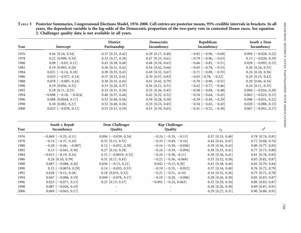
TABLE 3 Posterior Summaries, Congressional Elections Model, 1976-2000. Cell entries are posterior means, 95% credible intervals in brackets. In allyears, the dependent variable is the log-odds of the Democratic proportion of the two-party vote in contested House races. See equation2. Challenger quality data is not available in all years.

Year InterceptDistrict

PartisanshipDemocraticIncumbency

RepublicanIncumbency

South x DemIncumbency

1976 0.44 [0.34, 0.54] 0.37 [0.33, 0.42] 0.29 [0.17, 0.40] 20.82 [20.96, 20.68] 0.094 [20.028, 0.22]1978 0.22 [0.098, 0.34] 0.33 [0.27, 0.38] 0.47 [0.33, 0.61] 20.79 [20.96, 20.63] 0.13 [20.020, 0.29]1980 0.09 [20.03, 0.21] 0.43 [0.38, 0.48] 0.48 [0.34, 0.63] 20.66 [20.81, 20.51] 0.028 [20.095, 0.15]1982 0.19 [0.093, 0.28] 0.36 [0.31, 0.42] 0.54 [0.42, 0.66] 20.65 [20.78, 20.53] 0.38 [0.24, 0.53]1984 0.021 [20.14, 0.18] 0.38 [0.33, 0.43] 0.49 [0.32, 0.67] 20.71 [20.89, 20.55] 0.24 [0.10, 0.36]1986 0.033 [20.077, 0.14] 0.37 [0.32, 0.41] 0.70 [0.57, 0.83] 20.65 [-0.78, 20.52] 0.29 [0.15, 0.42]1988 0.078 [20.085, 0.24] 0.38 [0.33, 0.43] 0.61 [0.42, 0.79] 20.70 [20.90, 20.51] 0.20 [0.06, 0.34]1990 0.19 [0.056, 0.32] 0.33 [0.28, 0.37] 0.36 [0.21, 0.51] 20.62 [20.77, 20.46] 0.24 [0.11, 0.35]1992 0.18 [0.11, 0.25] 0.35 [0.31, 0.39] 0.35 [0.26, 0.45] 20.58 [20.69, 20.48] 0.094 [20.016, 0.20]1994 20.098 [20.18, 20.024] 0.40 [0.37, 0.44] 0.42 [0.32, 0.52] 20.54 [20.64, 20.45] 0.063 [20.025, 0.15]1996 0.088 [0.0044, 0.17] 0.52 [0.48, 0.56] 0.39 [0.28, 0.50] 20.39 [20.49, 20.29] 0.096 [20.031, 0.22]1998 0.18 [0.082, 0.27] 0.52 [0.48, 0.56] 0.33 [0.23, 0.45] 20.54 [20.65, 20.43] 0.028 [20.088, 0.15]2000 0.025 [20.078, 0.12] 0.55 [0.51, 0.59] 0.51 [0.39, 0.63] 20.41 [20.52, 20.30] 0.067 [20.041, 0.17]

YearSouth x RepubIncumbency

Dem ChallengerQuality

Rep ChallengerQuality nj r2

1976 20.069 [20.25, 0.11] 0.094 [20.039, 0.24] 20.24 [20.35, 20.13] 0.37 [0.35, 0.40] 0.78 [0.74, 0.81]1978 20.14 [20.37, 0.10] 0.33 [0.15, 0.53] 20.33 [20.49, 20.16] 0.44 [0.41, 0.47] 0.72 [0.68, 0.76]1980 20.28 [20.48, 20.087] 0.12 [20.052, 0.28] 20.16 [20.30, 20.036] 0.39 [0.36, 0.42] 0.80 [0.77, 0.83]1982 0.13 [20.041, 0.30] 0.27 [0.14, 0.39] 20.24 [20.39, 20.094] 0.38 [0.35, 0.41] 0.77 [0.73, 0.80]1984 20.015 [20.19, 0.16] 0.15 [20.0019, 0.32] 20.24 [20.38, -0.11] 0.38 [0.36, 0.41] 0.81 [0.78, 0.83]1986 0.24 [0.10, 0.39] 0.31 [0.17, 0.45] 20.21 [20.36, -0.069] 0.35 [0.32, 0.38] 0.85 [0.82, 0.87]1988 0.087 [20.088, 0.26] 0.036 [20.13, 0.21] 0.042 [20.13, 0.20] 0.41 [0.38, 0.44] 0.82 [0.79, 0.84]1990 0.15 [20.0074, 0.29] 0.14 [20.035, 0.33] 20.19 [20.35, 20.032] 0.37 [0.34, 0.40] 0.76 [0.72, 0.79]1992 0.028 [20.12, 0.18] 0.18 [0.033, 0.32] 20.21 [20.31, -0.10] 0.34 [0.32, 0.36] 0.75 [0.71, 0.78]1994 0.047 [20.088, 0.19] 0.049 [20.078, 0.17] 20.19 [20.29, 20.096] 0.28 [0.26, 0.30] 0.85 [0.83, 0.87]1996 0.023 [20.077, 0.13] 0.25 [0.13, 0.37] 20.092 [20.24, 0.063] 0.32 [0.29, 0.34] 0.86 [0.83, 0.87]1998 0.087 [20.026, 0.19] - - 0.28 [0.26, 0.30] 0.89 [0.87, 0.91]2000 0.069 [20.043, 0.17] - - 0.29 [0.27, 0.31] 0.90 [0.88, 0.91]

measurin

gdistrict-lev

elpartisa

nsh

ipwith

implica

tions

749

We also estimate challenger quality offsets, follow-ing the standard operationalization of a ‘‘quality’’challenger being one who has previously won anelection for public office (e.g., Jacobson and Kernell1983, 30). Our results indicate that quality challengersoften—but certainly not always—improve theirparty’s vote share. The 95% highest posterior densityintervals for these offsets frequently overlap zero (11out of 20 times for Democrats; eight out of 20 timesfor Republicans). But in a typical year, the estimatedoffset for a quality Republican challenger in an other-wise evenly poised race is on the order of three to fourpercentage points of vote share, and roughly the samefor a quality Democrat. Large estimates of challengerquality are obtained for 1978, for both parties (roughlycorresponding to seven to eight percentage points),representing the approximate peak of a not-especially-strong rise and fall in challenger quality offsets. Westress that these effects are small relative to theincumbency offsets we estimate, but, nonetheless, largeenough to be decisive in an otherwise close race. Wealso stress that challenger quality is, no doubt, endog-enous to district partisanship, with districts heavilyfavoring Democratic candidates less likely to attractquality Republican candidates, and vice-versa.

Presidential Elections

Results for our presidential elections models appearin Table 4. Two features stand out. First, the relation-ship between latent district partisanship and presi-dential elections outcomes has become considerablystronger over time; the discrimination parameter fordistrict partisanship ranges from a low of .32 in 1964to a maximum of .67 in 2000, with higher valueappearing in the 1980s and 1990s.13 In addition, ther2 for the presidential elections model generallyincreases over time, largely following the rise of thediscrimination parameters, reaching levels above .90for the 1976–2000 period. Taken together, this isevidence of the increasing partisan character ofelections; in turn, this reflects the fact that at leastat the district level, presidential election outcomes aremore highly correlated with one another across

successive elections, and with the outcomes of con-gressional elections.

Individual presidential elections have their ownunique aspects. For instance, presidential candidatesare hypothesized to receive a boost in their homestates because of personal popularity, see Lewis-Beckand Rice (1983) for details. We estimate home-stateoffsets in all districts in the home state of a particularpresidential or vice-presidential candidate. When twoor more of the candidates on the two major ticketsare from the same state, all four effects are notidentified, and we drop the vice-presidential dummyvariable in those years; the estimated effect in theseyears is an average of the two home-state effects. Weevaluate the estimated home-state effects by consid-ering a hypothetical district where the vote for thepresident is otherwise evenly split between the twomajor party candidates. Space constraints do notpermit a lengthy discussion of these estimates, butwe draw attention to the fact that Carter enjoyed thelargest home-state advantage (approximately 15points), while most other candidates clearly get someboost of around 5 to 10 points. Nixon is the onlycandidate with a clearly negative effect.14

Conclusion

Our pattern of results should provide reassurance toresearchers who have used district-level presidentialvote shares as a proxy for district-level partisanship.In the 1990s, presidential vote appears to be anexcellent proxy for district-level partisanship, ascongressional election outcomes and presidentialelection outcomes have become more highly corre-lated over the period we analyze (1952–2000). Inturn, this is consistent with the growing nationaliza-tion of elections noted by other scholars (e.g., Brady,Fiorina, and D’ Onofrio 2000). That is, while we findconsiderable variation in partisanship across districts,district-level vote shares in presidential and congres-sional elections have become more tightly tied topartisanship over the period we study. Net of theeffects of incumbency and challenger quality, con-gressional election outcomes are increasingly drivenby the same forces that determine presidential elec-tion outcomes, and vice-versa.

We again stress the flexibility of the model. Soas to generate good coverage across districts and

13The term ‘‘discrimination’’ parameter comes from the educa-tional testing literature, where a test item helps us discriminateamong test-subjects of higher and lower abilities; analogously,elections differ in the extent to which they convey informationabout varying levels of partisanship. The identifying restrictionthat district partisanship has a mean of zero and a standarddeviation of one across districts within any given decade allows usto make these over-time comparisons about the discriminationparameters.

14The negative estimate for George H.W. Bush in 1988 masks thehome-state boost for Lloyd Bentsen, the Democratic vice-presi-dential nominee from Texas.


TABLE 4 Posterior Summaries, Presidential Elections Model. Cell entries are the posterior means, 95% credible intervals in brackets. Dependentvariable in all years is the log-odds of the Democratic share of the two-party presidential vote; see equation 4. All four home state effectsare not jointly identified where two or more of the presidential and/or vice-presidential candidates are from the same state; in these casesthe vice-presidential effect is omitted.

Year Intercept District Partisanship Democrat Home State Republican Home State

1952 20.15 [20.17, 20.13] 0.47 [0.46, 0.49] 0.023 [20.055, 0.10] 20.32 [20.49, 20.15]1956 20.24 [20.26, 20.22] 0.47 [0.45, 0.49] 20.051 [20.14, 0.042] 20.055 [20.25, 0.13]1960 0.048 [0.023, 0.074] 0.39 [0.37, 0.41] 0.49 [0.36, 0.63] 0.023 [20.087, 0.13]1964 0.43 [0.38, 0.48] 0.32 [0.27, 0.37] 0.20 [20.010, 0.42] 20.24 [20.80, 0.35]1968 20.084 [20.28, 0.10] 0.45 [0.42, 0.48] 0.31 [0.074, 0.53] 0.056 [20.049, 0.17]1972 20.54 [20.57, 20.50] 0.38 [0.34, 0.41] 0.63 [0.12, 1.13] 0.30 [0.19, 0.42]1976 0.092 [0.078, 0.11] 0.44 [0.43, 0.46] 0.62 [0.47, 0.76] 20.23 [20.31, 20.15]1980 20.14 [20.16, 20.12] 0.54 [0.53, 0.56] 0.47 [0.29, 0.66] 20.11 [20.17, 20.034]1984 20.38 [20.40, 20.36] 0.55 [0.53, 0.56] 0.11 [0.012, 0.20] 20.066 [20.11, 20.024]1988 20.16 [20.18, 20.14] 0.54 [0.53, 0.56] 0.030 [20.051, 0.12] 0.38 [0.27, 0.50]1992 0.14 [0.13, 0.16] 0.52 [0.51, 0.54] 0.41 [0.23, 0.57] 0.042 [20.028, 0.12]1996 0.24 [0.23, 0.25] 0.62 [0.62, 0.63] 0.33 [0.20, 0.45] 20.23 [20.33, 20.12]2000 0.081 [0.067, 0.095] 0.67 [0.66, 0.69] 0.13 [20.017, 0.28] 20.17 [20.23, 20.11]

Year Democrat Vice-Pres Home State Republican Vice-Pres Home State nk r2

1952 0.30 [0.15, 0.42] 20.072 [20.15, 0.013] 0.13 [0.11, 0.15] 0.93 [0.91, 0.95]1956 0.17 [0.037, 0.30] 0.096 [20.0016, 0.19] 0.18 [0.16, 0.20] 0.87 [0.85, 0.90]1960 20.027 [20.13, 0.081] - 0.24 [0.22, 0.26] 0.73 [0.69, 0.77]1964 0.20 [20.16, 0.53] 0.31 [0.15, 0.47] 0.49 [0.45, 0.53] 0.33 [0.22, 0.43]1968 0.16 [20.30, 0.62] 0.097 [20.08, 0.28] 0.29 [0.26, 0.32] 0.70 [0.64, 0.76]1972 - 20.10 [20.36, 0.16] 0.37 [0.35, 0.40] 0.52 [0.44, 0.58]1976 0.19 [0.033, 0.34] 0.092 [20.057, 0.25] 0.13 [0.12, 0.15] 0.92 [0.90, 0.94]1980 0.24 [0.05, 0.43] 20.081 [20.17, 0.0037] 0.17 [0.15, 0.19] 0.91 [0.89, 0.93]1984 20.075 [20.12, 20.026] 0.27 [0.16, 0.39] 0.096 [0.081, 0.11] 0.97 [0.96, 0.98]1988 - 20.14 [20.22, 20.06] 0.10 [0.084, 0.11] 0.97 [0.96, 0.98]1992 0.15 [0.012, 0.28] 20.015 [20.12, 0.086] 0.15 [0.14, 0.16] 0.92 [0.91, 0.94]1996 0.061 [20.066, 0.18] 0.13 [0.09, 0.18] 0.07 [0.058, 0.083] 0.99 [0.98, 0.99]2000 0.14 [0.012, 0.25] 20.45 [20.74, 20.17] 0.13 [0.12, 0.14] 0.96 [0.96, 0.97]

measurin

gdistrict-lev

elpartisa

nsh

ipwith

implica

tions

751

elections, we use vote shares in congressional andpresidential elections as indicators of district-levelpartisanship, with district-level census aggregatesproviding additional information. Nothing precludesus from adding other indicators of district partisan-ship to the model; as mentioned above, these otherindicators might include state- or local-level electionoutcomes, Senate election outcomes, votes on ballotinitiatives, party registration data, or survey data,aggregated to districts. Replicating our model andanalysis at other levels of aggregation is anotherpromising line of work: recovering estimates ofstate-level or county-level partisanship seems feasibleand useful.

Finally, we concede that other researchers mighthave other ideas as to the nature of district partisan-ship and hence how to measure that concept. Ourconceptualization and operationalization is based onthe normal vote and so has strong, theoretical micro-foundations and a long lineage in the Americanpolitics literature. But we can imagine other research-ers preferring an approach that relied more heavilyon indicators of policy preferences per se or ideo-logical self-placements (say, from survey data, as wedo in the appendix), or voting on ballot initiatives orreferenda. These extensions are to be encouraged andare easily implemented with our modeling approach,a rigorous yet flexible methodology for combiningdisparate sources of information with which toestimate district partisanship.

Manuscript submitted 28 February 2007Manuscript accepted for publication 10 November 2007

References

Achen, Christopher. 1978. ‘‘Measuring Representation.’’ Ameri-can Journal of Political Science 22 (3): 475–510.

Achen, Christopher. 1979. ‘‘The Bias in Normal Vote Estimates.’’Political Methodology 6 (3): 343–56.

Adler, E. Scott. 2003. ‘‘Congressional District Data File, 1952–1996.’’ University of Colorado.

Adler, E. Scott, and John S. Lapinski. 1997. ‘‘Demand-SideTheroy and Congressional Committee Composition: A Con-stituency Characteristics Approach.’’ American Journal ofPolitical Science 41 (3): 895–918.

Aldrich, John H., and Richard D. McKelvey. 1977. ‘‘A Method ofScaling with Applications to the 1968 and 1972 PresidentialElections.’’ American Political Science Review 71 (1): 111–30.

Alford, J., and David W. Brady. 1993. ‘‘Personal and PartisanAdvantage in U.S. Elections, 1846–1992.’’ In Congress Recon-sidered, ed. Lawrence Dodd and Bruce Oppenheimer. 5th ed.Washington: Congressional Quartely Press, 141–57.

Ansolabehere, Stephen, and James M. Snyder. 2002. ‘‘TheIncumbency Advantage in U.S. Elections: An Analysis of State

and Federal Offices, 1942–2000.’’ Election Law Journal 1 (3):315–38.

Ansolabehere, Stephen, James M. Snyder Jr., and Charles StewartIII. 2000. ‘‘Old Voters, New Voters, and the Personal Vote:Using Redistricting to Measure the Incumbency Advantage.’’American Journal of Political Science 44 (1): 17–34.

Ansolabehere, Stephen, James M. Snyder Jr., and Charles StewartIII. 2001. ‘‘Candidate Positioning in U.S. House Elections.’’American Journal of Political Science 45 (1): 136–59.

Ardoin, Philip J., and James G. Garand. 2003. ‘‘MeasuringConstituency Ideology in U.S. House Districts: A Top-DownSimulation Approach.’’ Journal of Politics 65 (4): 1165–89.

Barone, Michael, and Grant Ujifusa. 1995. The Almanac ofAmerican Politics, 1996. Washington: National Journal Group.

Barone, Michael, and Richard E. Cohen. 2006. The Almanac ofAmerican Politics, 2006. Washington: National Journal Group.

Brady, David, Morris Fiorina, and Robert D’ Onofrio. 2000. ‘‘TheNationalization of Electoral Forces Revisited.’’ In Continuityand Change in House Elections, ed. David Brady, John Cogan,and Morris Fiorina. Stanford: Stanford University Press, 130–48.

Canes-Wrone, Brandice, John F. Cogan, and David W. Brady.2002. ‘‘Out of Step, Out of Office: Electoral Accountabilityand House Members’ Voting.’’ American Political ScienceReview 96 (1) 127–40.

Clinton, Joshua. 2007. ‘‘Representation in Congress: Constituentsand Roll Calls in the 106th House.’’ Journal of Politics 69 (2):455–67.

Clinton, Joshua D., Simon Jackman, and Douglas Rivers. 2004.‘‘The Statistical Analysis of Roll Call Data.’’ American PoliticalScience Review 98 (2): 355–70.

Converse, Philip E. 1996. ‘‘The Concepts of a Normal Vote.’’ InElections and the Political Order, ed. Angus Campbell, Philip E.Converse, Warren E. Miller, and Donald E. Stokes. New York:John Wiley and Sons, 9–39.

Cox, Gray W., and Jonathan N. Katz. 1999. ‘‘The Reapportion-ment Revolution and Bias in U.S. Congressional Elections.’’American Journal of Political Science 43 (3): 812–41.

Desposato, Scott W., and John R. Petrocik. 2003. ‘‘The VariableIncumbency Advantage: New Voters, Redistricting, and thePersonal Vote.’’ American Journal of Political Science 47 (1):18–32.

Duson, David B., Jesus Palomo, and Kenneth A. Bollen. 2007.‘‘Bayesian Structural Equation Modeling.’’ In Handbook ofLatent Variable and Related Models, ed. Sik-Yum Lee. Oxford:Elsevier, 163–88.

Erickson, Robert, and Gerald C. Wright. 1980. ‘‘Policy Repre-sentation of Constituency Interests.’’ Political Behavior 2 (1):91–106.

Erikson, Robert S. 1978. ‘‘Constituency Opinion and Congres-sional Behaviour: A Reexamination of the Miller-StokesRepresentation Data.’’ American Journal of Political Science22 (3): 511–35.

Gelman, Andrew, and Gray King. 1990. ‘‘Estimasting Incum-bency Advantage without Bias.’’ American Journal of PoliticalScience 34 (4): 1142–64.

Gerber, Elisabeth R., and Jeffrey B. Lewis. 2004. ‘‘Beyond theMedian: Voter Preferences, District Heterogeneity, and Polit-ical Representation.’’ Journal of Political Economy 112 (6):1364–83.

Goldenberg, Edie N., and Michael W. Traugott. 1981. ‘‘NormalVote Analysis of U.S. Congressional Elections.’’ LegislativeStudies Quarterly 6 (2): 247–57.


Hox, Joop. 2002.Multilevel Analysis: Techniques and Applications.Mahwah, NJ: Lawrence Erlbaum.

Jackman, Simon D. 2000. ‘‘Estimation and Inference via BayesianSimulation: An Introducdtion to Markov Chain MonteCarlo.’’ American Journal of Political Science 44 (2): 375–404.

Jacobson, Gray C., and Samuel Kernell. 1983. Strategy and Choicein Congressional Elections. New Haven: Yale University Press.

Joreskog, Karl G. 2000. Latent Variable Scores and Their Uses.Technical report Scientific Software International, Inc. Lin-colnwood, Illinois: http://www.ssicentral.com/lisrel/techdocs/lvscores.pdf.

Kalt, Joseph P., and Mark A. Zupan. 1984. ‘‘Capture andIdeology in the Economic Theory of Politics.’’ AmericanEconomic Review 74 (3): 279–300.

Katz, Jonathan N., and Gray King. 1999. ‘‘A Statistical Model forMultiparty Electoral Data.’’ American Political Science Review93 (1): 15–32.

Kawato, Sadafumi. 1987. ‘‘Nationalization and Partisan Realign-ment in Congressional Elections.’’ American Political ScienceReview 81 (4): 1235–45.

Lewis-Beck, Michael, and Tom Rice. 1983. ‘‘Localism in Presi-dential Elections: The Home-State Advantage.’’ AmericanJournal of Political Science 27 (3): 548–56.

Mardia, Kanti V., John T. Kent, and John M. Bibby. 1979.Multivariate Analysis. San Diego: Academic Press.

McCarty, Nolan, Keith T. Poole, and Howard Rosenthal. 2003.‘‘Political Polarization and Income Inequality.’’ Unpublishedmanuscript. Princeton University.

Miller, Warren E., and Donald E. Stokes. 1963. ‘‘ConstituencyInfluence in Congress.’’ American Political Science Review 57(1): 45–56.

Peltzman, Sam. 1984. ‘‘Constituent Interest and CongressionalVoting.’’ Journal of Law and Economics 27 (1): 181–210.

Petrocik, John R. 1989. ‘‘An Expected Party Vote: New Datafor an Old Concept.’’ American Journal of Political Science 33(1): 44–66.

Skrondal, Anders, and Sophia Rabe-Hesketh. 2004. GeneralizedLatent Variable Modeling: Multi-level, Longitudinal, andStructural Equation Models. Boca Raton. Chapman andHall/CRC.

Snydser, Jr. James M. 2005. ‘‘Estimating the Distribution of VoterPreferences Using Partially Aggregated Voting Data.’’ ThePolitical Methodologist 13 (1): 2–5.

Snyder, Jr. James M., and Tim Groseclose. 2000. ‘‘EstimatingParty Influence in Congressional Roll-Call Voting.’’ AmericanJournal of Political Science 44 (2): 187–205.

Stoker, Laura, and Jake Bowers. 2002. ‘‘Designing Multi-levelStudies: Sampling Voters and Electoral Contexts.’’ ElectoralStudies 21 (2): 235–67.

Wright, Gerald C., Robert S. Erickson, and John P. McIver. 1985.‘‘Measuring State Partisanship and Ideology with SurveyData.’’ Journal of politics 47 (2): 469–89.

Matthew S. Levendusky is assistant professor ofpolitical science, University of Pennsylvania, Phila-delphia, PA 19104. Jeremy C. Pope is assistantprofessor of political science and research fellow,Center for the Study of Elections and Democracy,Brigham Young University, Provo, UT 84602. SimonD. Jackman is professor of political science andDirector of Political Science and ComputationalLaboratory, Stanford University, Stanford, CA 94305.


Documents

Measuring District-Level Partisanship with Implications ... · nu m ber of congressional districts is ve ry difÞ cu lt, give n the data-gathering tech no logies an d resea rch bu