Embed Size (px)
Citation preview
Measures of multivariate skewness and kurtosis
in high-dimensional framework
Takuma SUMIKAWA∗ Kazuyuki KOIZUMI† Takashi SEO‡
Abstract
In this paper, we propose new definitions for multivariate skewness and kurtosis when thecovariance matrix has a block diagonal structure. These measures are based on the ones ofMardia (1970). We give the expectations and the variances for new multivariate sample mea-sures of skewness and kurtosis. Further, we derive asymptotic distributions of statistics bynew measures under multivariate normality. To evaluate accuracy of these statistics, numer-ical results are given by the Monte Carlo simulation. We consider the problem estimating forcovariance structure. Pavlenko, Bjorkstrom and Tillander (2012) consider a method whichapproximate the inverse covariance matrix to block diagonal structure via gLasso. In thispaper, we propose an improvement of Pavlenko, Bjorkstrom and Tillander (2012)’s methodby using AIC. Finally, numerical results are shown in order to investigate probability thatthe new method select true model for covariance structure.
Key Words and Phrases: Multivariate Skewness; Multivariate Kurtosis; Normality test; Co-variance structure approximation; Block diagonal matrix; AIC.
1 Introduction
In multivariate statical analysis, normality for sample is assumed in many cases. Hence,assessing for multivariate normality is an important problem. The graphical method and thestatistical hypothesis testing are considered to this problem by many authors (see, e.g. Henze(2002); Thode (2002)). From aspects of calculation cost and simplicity, we focus on the testingtheory based on multivariate skewness and kurtosis. There are various definitions of multivariateskewness and kurtosis (Mardia (1970), Malkovich and Afifi (1973), Srivastava (1984) and soon.). Mardia (1970, 1974) defined multivariate skewness and kurtosis as a natural extension ofunivariate case. To assess multivariate normality, sample measures of multivariate skewness andkurtosis have been defined and their asymptotic distributions under the multivariate normalityhave been given in Mardia (1970). Srivastava (1984) also has considered another definition forthe sample measures by using principal component scores and derived their asymptotic nulldistributions. Recently, the sample measure of multivariate kurtosis of the form containing
∗Dept. of Mathematical Information Science, Graduate School of Science, Tokyo University of Science, Kagu-razaka 1-3, Shinjuku-ku, Tokyo 162-8601, Japan
†Dept. of International College of Arts and Sciences, Yokohama City University, Seto 22-2, Kanazawa-ku,Yokohama city, Kanagawa 236-0027, Japan
‡Dept. of Mathematical Information Science, Faculty of Science, Tokyo University of Science, Kagurazaka 1-3,Shinjuku-ku, Tokyo 162-8601, Japan
1
Mardia (1970) and Srivastava (1984) has been proposed by Miyagawa et al. (2012). Recently,Koizumi et al. (2009) proposed an omnibus test statistic MJB by using Mardia’s and Srivastava’sskewness and kurtosis for assessing multivariate normality. Improvements of MJB test statistichave been discussed by many authors (see, e.g. Enomoto et al. (2012); Koizumi et al. (2013)).
These theory have been considered when the sample size N is larger than the dimension p.Since sample covariance matrix S is singular, it cannot be used when the dimension p is largerthan sample size N . In this paper, we propose new measures of multivariate skewness andkurtosis when the covariance structure is a block diagonal matrix and derive their asymptoticdistributions under the multivariate normality.
Further, we consider to estimate for inverse covariance matrix to a block diagonal structure.Pavlenko et al. (2012) propose a gLasso estimator of inverse covariance matrix Ξ. Similarestimates of Ξ were also considered in Rothman et al. (2008) and Rutimann et al. (2009).By the Pavlenko’s method, Ξ may be estimated as incomplete block diagonal matrix. In thispaper, we give an improvement of Pavlenko’s method by using Akaike’s information criterion(AIC). AIC is proposed by Akaike (1973, 1974) as an estimator of the risk function based onKullback-Leibler information (Kullback and Leibler (1951)). It is used for selecting the optimalmodel among the candidate models.
The organization of this paper is as following. In Section 2, we examine the definition ofMardia’s (1970) multivariate skewness and kurtosis and their asymptotic distributions under themultivariate normality. In Section 3, we propose new multivariate skewness and kurtosis andderive their asymptotic distributions under the multivariate normality. In Section 4, we considerthe Pavlenko’s method for the block diagonal approximation and propose an AIC-method whichis an improvement of Pavlenko’s method by using AIC. In Section 5, numerical results aregiven by Monte Carlo simulation to evaluate the accuracy of the upper percentage points fornew statistics proposed in Section 3. Further, we investigate correct selection rate (CSR) ofAIC-method proposed in Section 4.
2 Mardia’s multivariate skewness and multivariate kurtosis
First, we discuss measures of multivariate skewness and multivariate kurtosis defined byMardia (1970). Let x and y be random p-vectors with the mean vector µ and the covariancematrix Σ. Then Mardia (1970) has defined population measures of multivariate skewness andkurtosis as
β1 = E[{(x− µ)′Σ−1(y − µ)}3], (2.1)
β2 = E[{(x− µ)′Σ−1(x− µ)}2], (2.2)
where x and y are independent and identical random vectors. We note that β1 = 0 and β2 =p(p + 2) hold under multivariate normality. These measures are invariant under a nonsingulartransformation
x = Au+ b, (2.3)
where A is a nonsingular p × p matrix and b is a p-vector. Let x1,x2, . . . ,xN be sampleobservation vectors of size N from a multivariate population with the mean vector µ and the
2

covariance matrix Σ. And let x and S be the sample mean vector and the sample covariancematrix based on sample size N as follows:
x =1
N
N∑j=1
xj ,
S =1
N
N∑j=1
(xj − x) (xj − x)′ ,
respectively. Then the sample measures of multivariate skewness and multivariate kurtosis inMardia (1970) are defined as
b1 =1
N2
N∑i=1
N∑j=1
{(xi − x)′S−1(xj − x)}3, (2.4)
b2 =1
N
N∑i=1
{(xi − x)′S−1(xi − x)}2. (2.5)
These measures are invariant under a nonsingular transformation in (2.3). Then Mardia (1970)obtained the following lemma.
Lemma 1. (Mardia (1970)) The expectation of b1 in (2.4) and the expectation and the vari-ance of b2 in (2.5) under the multivariate normal population Np(µ,Σ) are given by
E[b1] =1
Np(p+ 1)(p+ 2) + o(N−1), (2.6)
E[b2] =N − 1
N + 1p(p+ 2), (2.7)
Var[b2] =8
Np(p+ 2) + o(N−1). (2.8)
Proof. Mardia (1970) rewrite (2.4) as
b1 =
p∑r=1
p∑r′=1
p∑s=1
p∑s′=1
p∑t=1
p∑t′=1
Srr′Sss′Stt′ , (2.9)
where
S−1 = {Sij} and M(rst)111 =
1
N
N∑i=1
(xri − xr)(xsi − xs)(xti − xt).
Let x1,x2, . . . ,xN be a random sample from Np(µ,Σ). Since b1 is invariant under linear trans-formation, we assume µ = 0 and Σ = Ip. S converges to Σ in probability. Therefore, from (2.9),we get
b1P−→∑r,s,t
{M (rst)111 }
2, (2.10)
3
in probability. We have
b1P−→ {M (1)
3 }2+ · · ·+ 3{M (12)
21 }2+ · · ·+ 6{M (123)
111 }2+ · · · (2.11)
in probability by writing M(rrr)111 = M
(r)3 and M
(rss)111 = M
(rs)12 (r = s) in (2.10). Using the
normality of the vector {M (1)3 , . . . ,M
(12)21 , . . . ,M
(123)111 , . . .}, Mardia (1970) derive
E[b1] =1
Np(p+ 1)(p+ 2) + o(N−1).
Let x∗r = (xr1, xr2, . . . , xrN )′ (r = 1, 2, . . . , p). We transform x∗
r to ξ∗r = (ξr1, ξr2, . . . , ξrN )′ byan orthogonal transformation ξ∗r = Cx∗
r (r = 1, 2, . . . , p), where C is an orthogonal matrix withthe first row as (1/
√N, 1/
√N, . . . , 1/
√N) and the second row as (−a, . . . ,−a, 1/
√Na), a being
1/√
N(N − 1). Then we find
E[b2] = (N − 1)2E[y],
where
y = ξ′2(
N∑t=2
ξtξ′t)−1ξ2 with ξ
′t = (ξ1t, ξ2t, . . . , ξpt)
′ (t = 2, . . . , N).
From Rao (1965, p. 459), we find the probability density function of y. Hence, Mardia (1970)give
E[b2] =N − 1
N + 1p(p+ 2).
Let S = I + S∗ so that to order N−1,E(S∗) = 0. On using
S−1 = (I + S∗)−1 = I − S∗ + S∗2 − · · ·
in (2.5), we obtain that
b2 =1
N
N∑i=1
{(xi − x)′(xi − x)}2 − 2
N
N∑i=1
(xi − x)′(xi − x)(xi − x)′S∗(xi − x) + · · · . (2.12)
Further, we rewrite (2.12) as
b2 =
p∑i=1
M(i)4 +
∑i=j
M(ij)22 − 2
p∑i=1
M(i)∗2 M
(i)4 − 2
∑i=j
M(j)∗2 M
(ij)22 − 2
p∑i=1
∑j =k
M(jk)∗11 M
(ijk)211 . . . ,
(2.13)
where
M(j1,...,js)i1,...,is
=1
N
N∑i=1
{s∏
r=1
(xjri − xjr)ir}, M
(i)∗2 = S∗
ii, M(ij)∗11 = S∗
ij
with S∗ = {S∗ij}. Using the normality of the vector M
(j1,...,js)i1,...,is
, Mardia (1970) derive
Var[b2] =8
Np(p+ 2) + o(N−1).
4
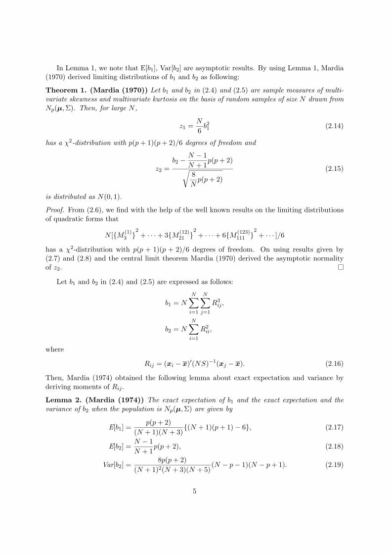
In Lemma 1, we note that E[b1], Var[b2] are asymptotic results. By using Lemma 1, Mardia(1970) derived limiting distributions of b1 and b2 as following:
Theorem 1. (Mardia (1970)) Let b1 and b2 in (2.4) and (2.5) are sample measures of multi-variate skewness and multivariate kurtosis on the basis of random samples of size N drawn fromNp(µ,Σ). Then, for large N ,
z1 =N
6b21 (2.14)
has a χ2-distribution with p(p+ 1)(p+ 2)/6 degrees of freedom and
z2 =b2 −
N − 1
N + 1p(p+ 2)√
8
Np(p+ 2)
(2.15)
is distributed as N(0, 1).
Proof. From (2.6), we find with the help of the well known results on the limiting distributionsof quadratic forms that
N [{M (1)3 }
2+ · · ·+ 3{M (12)
21 }2+ · · ·+ 6{M (123)
111 }2+ · · · ]/6
has a χ2-distribution with p(p + 1)(p + 2)/6 degrees of freedom. On using results given by(2.7) and (2.8) and the central limit theorem Mardia (1970) derived the asymptotic normalityof z2.
Let b1 and b2 in (2.4) and (2.5) are expressed as follows:
b1 = N
N∑i=1
N∑j=1
R3ij ,
b2 = N
N∑i=1
R2ii,
where
Rij = (xi − x)′(NS)−1(xj − x). (2.16)
Then, Mardia (1974) obtained the following lemma about exact expectation and variance byderiving moments of Rij .
Lemma 2. (Mardia (1974)) The exact expectation of b1 and the exact expectation and thevariance of b2 when the population is Np(µ,Σ) are given by
E[b1] =p(p+ 2)
(N + 1)(N + 3){(N + 1)(p+ 1)− 6}, (2.17)
E[b2] =N − 1
N + 1p(p+ 2), (2.18)
Var[b2] =8p(p+ 2)
(N + 1)2(N + 3)(N + 5)(N − p− 1)(N − p+ 1). (2.19)
5
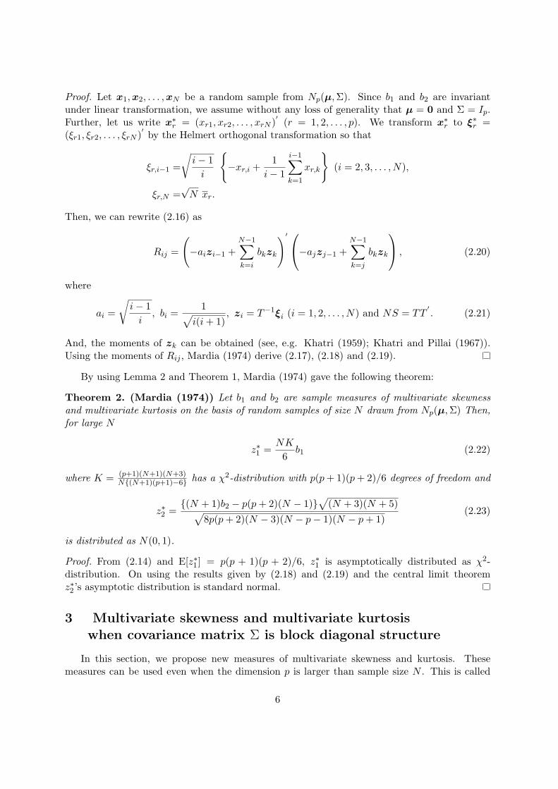
Proof. Let x1,x2, . . . ,xN be a random sample from Np(µ,Σ). Since b1 and b2 are invariantunder linear transformation, we assume without any loss of generality that µ = 0 and Σ = Ip.Further, let us write x∗
r = (xr1, xr2, . . . , xrN )′(r = 1, 2, . . . , p). We transform x∗
r to ξ∗r =(ξr1, ξr2, . . . , ξrN )
′by the Helmert orthogonal transformation so that
ξr,i−1 =
√i− 1
i
{−xr,i +
1
i− 1
i−1∑k=1
xr,k
}(i = 2, 3, . . . , N),
ξr,N =√N xr.
Then, we can rewrite (2.16) as
Rij =
(−aizi−1 +
N−1∑k=i
bkzk
)′−ajzj−1 +N−1∑k=j
bkzk
, (2.20)
where
ai =
√i− 1
i, bi =
1√i(i+ 1)
, zi = T−1ξi (i = 1, 2, . . . , N) and NS = TT′. (2.21)
And, the moments of zk can be obtained (see, e.g. Khatri (1959); Khatri and Pillai (1967)).Using the moments of Rij , Mardia (1974) derive (2.17), (2.18) and (2.19).
By using Lemma 2 and Theorem 1, Mardia (1974) gave the following theorem:
Theorem 2. (Mardia (1974)) Let b1 and b2 are sample measures of multivariate skewnessand multivariate kurtosis on the basis of random samples of size N drawn from Np(µ,Σ) Then,for large N
z∗1 =NK
6b1 (2.22)
where K = (p+1)(N+1)(N+3)N{(N+1)(p+1)−6} has a χ2-distribution with p(p+ 1)(p+ 2)/6 degrees of freedom and
z∗2 ={(N + 1)b2 − p(p+ 2)(N − 1)}
√(N + 3)(N + 5)√
8p(p+ 2)(N − 3)(N − p− 1)(N − p+ 1)(2.23)
is distributed as N(0, 1).
Proof. From (2.14) and E[z∗1 ] = p(p + 1)(p + 2)/6, z∗1 is asymptotically distributed as χ2-distribution. On using the results given by (2.18) and (2.19) and the central limit theoremz∗2 ’s asymptotic distribution is standard normal.
3 Multivariate skewness and multivariate kurtosiswhen covariance matrix Σ is block diagonal structure
In this section, we propose new measures of multivariate skewness and kurtosis. Thesemeasures can be used even when the dimension p is larger than sample size N . This is called
6
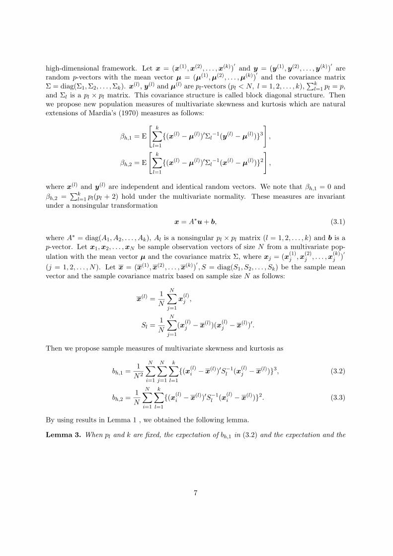
high-dimensional framework. Let x = (x(1),x(2), . . . ,x(k))′and y = (y(1),y(2), . . . ,y(k))
′are
random p-vectors with the mean vector µ = (µ(1),µ(2), . . . ,µ(k))′and the covariance matrix
Σ = diag(Σ1,Σ2, . . . ,Σk). x(l), y(l) and µ(l) are pl-vectors (pl < N, l = 1, 2, . . . , k),
∑kl=1 pl = p,
and Σl is a pl × pl matrix. This covariance structure is called block diagonal structure. Thenwe propose new population measures of multivariate skewness and kurtosis which are naturalextensions of Mardia’s (1970) measures as follows:
βh,1 = E
[k∑
l=1
{(x(l) − µ(l))′Σl−1(y(l) − µ(l))}3
],
βh,2 = E
[k∑
l=1
{(x(l) − µ(l))′Σl−1(x(l) − µ(l))}2
],
where x(l) and y(l) are independent and identical random vectors. We note that βh,1 = 0 and
βh,2 =∑k
l=1 pl(pl + 2) hold under the multivariate normality. These measures are invariantunder a nonsingular transformation
x = A∗u+ b, (3.1)
where A∗ = diag(A1, A2, . . . , Ak), Al is a nonsingular pl × pl matrix (l = 1, 2, . . . , k) and b is ap-vector. Let x1,x2, . . . ,xN be sample observation vectors of size N from a multivariate pop-
ulation with the mean vector µ and the covariance matrix Σ, where xj = (x(1)j ,x
(2)j , . . . ,x
(k)j )
′
(j = 1, 2, . . . , N). Let x = (x(1),x(2), . . . ,x(k))′, S = diag(S1, S2, . . . , Sk) be the sample mean
vector and the sample covariance matrix based on sample size N as follows:
x(l) =1
N
N∑j=1
x(l)j ,
Sl =1
N
N∑j=1
(x(l)j − x(l))(x
(l)j − x(l))′.
Then we propose sample measures of multivariate skewness and kurtosis as
bh,1 =1
N2
N∑i=1
N∑j=1
k∑l=1
{(x(l)i − x(l))′S−1
l (x(l)j − x(l))}3, (3.2)
bh,2 =1
N
N∑i=1
k∑l=1
{(x(l)i − x(l))′S−1
l (x(l)i − x(l))}2. (3.3)
By using results in Lemma 1 , we obtained the following lemma.
Lemma 3. When pl and k are fixed, the expectation of bh,1 in (3.2) and the expectation and the
7

variance of bh,2 in (3.3) when the population is Np(µ,Σ) are given by
E[bh,1] =1
N
k∑l=1
pl(pl + 1)(pl + 2) + o(N−1), (3.4)
E[bh,2] =N − 1
N + 1
k∑l=1
pl(pl + 2), (3.5)
Var[bh,2] =8
N
k∑l=1
pl(pl + 2) + o(N−1). (3.6)
Proof. Let x = (x(1),x(2), . . . ,x(k))′be a random vectors from Np(µ,Σ), where µ = (µ(1),µ(2),
. . . ,µ(k))′and Σ = diag(Σ1,Σ2, . . . ,Σk). x(l), y(l) and µ(l) are pl-vectors (pl < N, l =
1, 2, . . . , k),∑k
l=1 pl = p, and Σl is a pl × pl matrix. The probability density function of xis defined as
f(x) =1
(2π)p2 |Σ|
12
exp
[−1
2(x− µ)
′Σ−1(x− µ)
]. (3.7)
Since (x− µ)′Σ−1(x− µ) =
∑kl=1(x
(l) − µ(l))′Σ−1l (x(l) − µ(l)) and |Σ| =
∏kl=1 |Σl|, we rewrite
(3.7) as
f(x) =
k∏l=1
1
(2π)pl2 |Σl|
12
exp
[−1
2(x(l) − µ(l))
′Σ−1l (x(l) − µ(l))
].
Hence, we find the independence of x(l) and x(l′) (l = l′, l, l′ = 1, 2, . . . , k). By using results inLemma 1 and independence of x(l) and x(l′) (l = l′, l, l′ = 1, 2, . . . , k), we obtain (3.4), (3.5) and(3.6).
By using Lemma 3, we derived the following theorem:
Theorem 3. Let bh,1 and bh,2 in (3.2) and (3.3) are sample measures of multivariate skewnessand multivariate kurtosis on the basis of random samples of size N drawn from Np(µ,Σ) Then,for large N ,
zh,1 =N
6bh,1 (3.8)
has a χ2-distribution with∑k
l=1 pl(pl + 1)(pl + 2)/6 degrees of freedom and
zh,2 =
bh,2 −N − 1
N + 1
k∑l=1
pl(pl + 2)√8
N
k∑l=1
pl(pl + 2)
(3.9)
is distributed as N(0, 1).
Proof. From Theorem 1, we derive (3.8). On using the results given by (3.5) and (3.6) and thecentral limit theorem we find that (3.9).
8
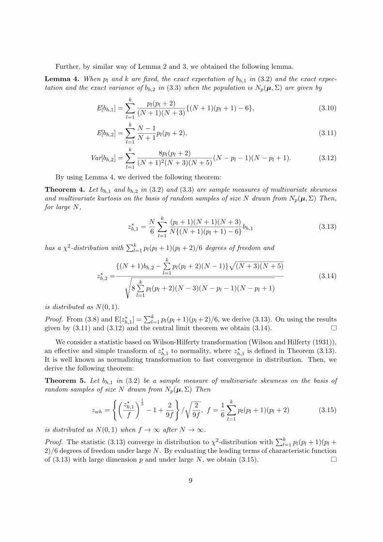
Further, by similar way of Lemma 2 and 3, we obtained the following lemma.
Lemma 4. When pl and k are fixed, the exact expectation of bh,1 in (3.2) and the exact expec-tation and the exact variance of bh,2 in (3.3) when the population is Np(µ,Σ) are given by
E[bh,1] =
k∑l=1
pl(pl + 2)
(N + 1)(N + 3){(N + 1)(pl + 1)− 6}, (3.10)
E[bh,2] =
k∑l=1
N − 1
N + 1pl(pl + 2), (3.11)
Var[bh,2] =k∑
l=1
8pl(pl + 2)
(N + 1)2(N + 3)(N + 5)(N − pl − 1)(N − pl + 1). (3.12)
By using Lemma 4, we derived the following theorem:
Theorem 4. Let bh,1 and bh,2 in (3.2) and (3.3) are sample measures of multivariate skewnessand multivariate kurtosis on the basis of random samples of size N drawn from Np(µ,Σ) Then,for large N ,
z∗h,1 =N
6
k∑l=1
(pl + 1)(N + 1)(N + 3)
N{(N + 1)(pl + 1)− 6}bh,1 (3.13)
has a χ2-distribution with∑k
l=1 pl(pl + 1)(pl + 2)/6 degrees of freedom and
z∗h,2 =
{(N + 1)bh,2 −k∑
l=1
pl(pl + 2)(N − 1)}√
(N + 3)(N + 5)√8
k∑l=1
pl(pl + 2)(N − 3)(N − pl − 1)(N − pl + 1)
(3.14)
is distributed as N(0, 1).
Proof. From (3.8) and E[z∗h,1] =∑k
l=1 pl(pl+1)(pl+2)/6, we derive (3.13). On using the resultsgiven by (3.11) and (3.12) and the central limit theorem we obtain (3.14).
We consider a statistic based on Wilson-Hilferty transformation (Wilson and Hilferty (1931)),an effective and simple transform of z∗h,1 to normality, where z∗h,1 is defined in Theorem (3.13).It is well known as normalizing transformation to fast convergence in distribution. Then, wederive the following theorem:
Theorem 5. Let bh,1 in (3.2) be a sample measure of multivariate skewness on the basis ofrandom samples of size N drawn from Np(µ,Σ) Then
zwh =
{(z∗h,1f
) 13
− 1 +2
9f
}/
√2
9f, f =
1
6
k∑l=1
pl(pl + 1)(pl + 2) (3.15)
is distributed as N(0, 1) when f → ∞ after N → ∞.
Proof. The statistic (3.13) converge in distribution to χ2-distribution with∑k
l=1 pl(pl + 1)(pl +2)/6 degrees of freedom under large N . By evaluating the leading terms of characteristic functionof (3.13) with large dimension p and under large N , we obtain (3.15).
9
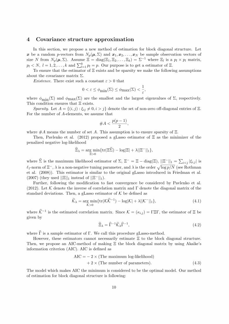
4 Covariance structure approximation
In this section, we propose a new method of estimation for block diagonal structure. Letx be a random p-vectors from Np(µ,Σ) and x1,x2, . . . ,xN be sample observation vectors ofsize N from Np(µ,Σ). Assume Ξ = diag(Ξ1,Ξ2, . . . ,Ξk) = Σ−1 where Ξl is a pl × pl matrix,
pl < N, l = 1, 2, . . . , k and∑k
l=1 pl = p. Our purpose is to get a estimator of Ξ.To ensure that the estimator of Ξ exists and be sparsity we make the following assumptions
about the covariance matrix Σ.Existence. There exist such a constant ε > 0 that
0 < ε ≤ ϕmin(Σ) ≤ ϕmax(Σ) <1
ε,
where ϕmin(Σ) and ϕmax(Σ) are the smallest and the largest eigenvalues of Σ, respectively.This condition ensures that Ξ exists.
Sparsity. Let A = {(i, j) : ξij = 0, i > j} denote the set of non-zero off-diagonal entries of Ξ.For the number of A-elements, we assume that
#A <p(p− 1)
2,
where #A means the number of set A. This assumption is to ensure sparsity of Ξ.Then, Pavlenko et al. (2012) proposed a gLasso estimator of Ξ as the minimizer of the
penalized negative log-likelihood
Ξλ = arg minΞ>0
{tr(ΞΣ)− log|Ξ|+ λ||Ξ−||1},
where Σ is the maximum likelihood estimator of Σ, Ξ− = Ξ − diag(Ξ), ||Ξ−||1 =∑
i<j |ξi,j | isℓ1-norm of Ξ−, λ is a non-negative tuning parameter, and λ is the order
√log p/N (see Rothman
et al. (2008)). This estimator is similar to the original gLasso introduced in Friedman et al.(2007) (they used ||Ξ||1 instead of ||Ξ−||1).
Further, following the modification to fast convergence be considered by Pavlenko et al.(2012). Let K denote the inverse of correlation matrix and Γ denote the diagonal matrix of thestandard deviations. Then, a gLasso estimator of K be defined as
Kλ = arg minK>0
{tr(KK−1)− log|K|+ λ||K−||1}, (4.1)
where K−1 is the estimated correlation matrix. Since K = (κi,j) = ΓΞΓ, the estimator of Ξ begiven by
Ξλ = Γ−1KλΓ−1, (4.2)
where Γ is a sample estimator of Γ. We call this procedure gLasso-method.However, these estimators cannot necessarily estimate Ξ to the block diagonal structure.
Then, we propose an AIC-method of making Ξ the block diagonal matrix by using Akaike’sinformation criterion (AIC). AIC is defined as
AIC =− 2× (The maximum log-likelihood)
+ 2× (The number of parameters). (4.3)
The model which makes AIC the minimum is considered to be the optimal model. Our methodof estimation for block diagonal structure is following:
10
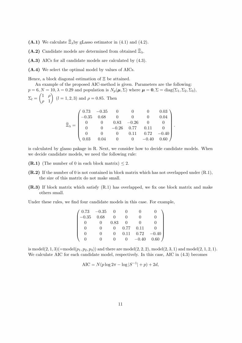
(A.1) We calculate Ξλby gLasso estimator in (4.1) and (4.2).
(A.2) Candidate models are determined from obtained Ξλ.
(A.3) AICs for all candidate models are calculated by (4.3).
(A.4) We select the optimal model by values of AICs.
Hence, a block diagonal estimation of Ξ be attained.An example of the proposed AIC-method is given. Parameters are the following:
p = 6, N = 10, λ = 0.29 and population is Np(µ,Σ) where µ = 0,Σ = diag(Σ1,Σ2,Σ3),
Σl =
(1 ρρ 1
)(l = 1, 2, 3) and ρ = 0.85. Then
Ξλ =
0.73 −0.35 0 0 0 0.03−0.35 0.68 0 0 0 0.04
0 0 0.83 −0.26 0 00 0 −0.26 0.77 0.11 00 0 0 0.11 0.72 −0.40
0.03 0.04 0 0 −0.40 0.60
.
is calculated by glasso pakage in R. Next, we consider how to decide candidate models. Whenwe decide candidate models, we need the following rule:
(R.1) (The number of 0 in each block matrix) ≤ 2.
(R.2) If the number of 0 is not contained in block matrix which has not overlapped under (R.1),the size of this matrix do not make small.
(R.3) If block matrix which satisfy (R.1) has overlapped, we fix one block matrix and makeothers small.
Under these rules, we find four candidate models in this case. For example,
0.73 −0.35 0 0 0 0−0.35 0.68 0 0 0 0
0 0 0.83 0 0 00 0 0 0.77 0.11 00 0 0 0.11 0.72 −0.400 0 0 0 −0.40 0.60
is model(2, 1, 3)(=model(p1, p2, p3)) and there are model(2, 2, 2), model(2, 3, 1) and model(2, 1, 2, 1).We calculate AIC for each candidate model, respectively. In this case, AIC in (4.3) becomes
AIC = N(p log 2π − log |S−1|+ p) + 2d,
11
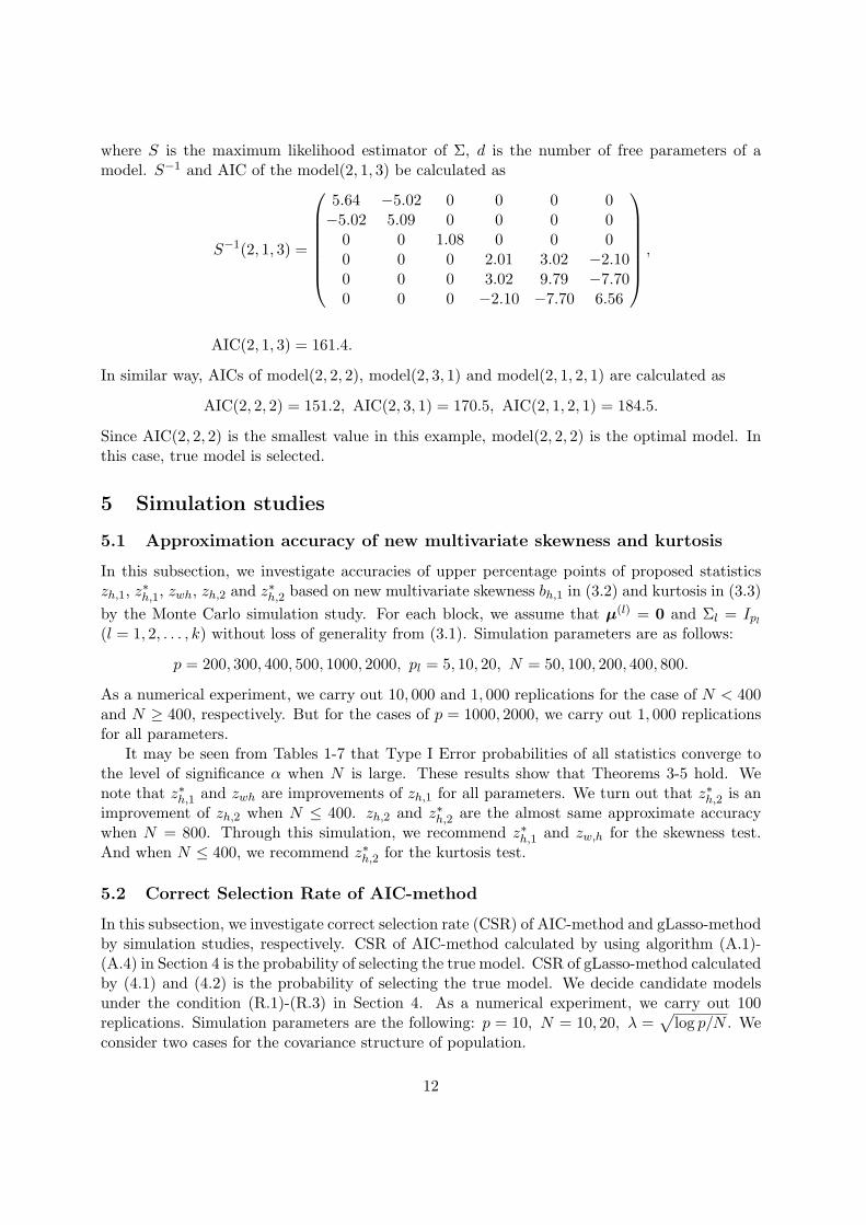
where S is the maximum likelihood estimator of Σ, d is the number of free parameters of amodel. S−1 and AIC of the model(2, 1, 3) be calculated as
S−1(2, 1, 3) =
5.64 −5.02 0 0 0 0−5.02 5.09 0 0 0 0
0 0 1.08 0 0 00 0 0 2.01 3.02 −2.100 0 0 3.02 9.79 −7.700 0 0 −2.10 −7.70 6.56
,
AIC(2, 1, 3) = 161.4.
In similar way, AICs of model(2, 2, 2), model(2, 3, 1) and model(2, 1, 2, 1) are calculated as
AIC(2, 2, 2) = 151.2, AIC(2, 3, 1) = 170.5, AIC(2, 1, 2, 1) = 184.5.
Since AIC(2, 2, 2) is the smallest value in this example, model(2, 2, 2) is the optimal model. Inthis case, true model is selected.
5 Simulation studies
5.1 Approximation accuracy of new multivariate skewness and kurtosis
In this subsection, we investigate accuracies of upper percentage points of proposed statisticszh,1, z
∗h,1, zwh, zh,2 and z∗h,2 based on new multivariate skewness bh,1 in (3.2) and kurtosis in (3.3)
by the Monte Carlo simulation study. For each block, we assume that µ(l) = 0 and Σl = Ipl(l = 1, 2, . . . , k) without loss of generality from (3.1). Simulation parameters are as follows:
p = 200, 300, 400, 500, 1000, 2000, pl = 5, 10, 20, N = 50, 100, 200, 400, 800.
As a numerical experiment, we carry out 10, 000 and 1, 000 replications for the case of N < 400and N ≥ 400, respectively. But for the cases of p = 1000, 2000, we carry out 1, 000 replicationsfor all parameters.
It may be seen from Tables 1-7 that Type I Error probabilities of all statistics converge tothe level of significance α when N is large. These results show that Theorems 3-5 hold. Wenote that z∗h,1 and zwh are improvements of zh,1 for all parameters. We turn out that z∗h,2 is animprovement of zh,2 when N ≤ 400. zh,2 and z∗h,2 are the almost same approximate accuracywhen N = 800. Through this simulation, we recommend z∗h,1 and zw,h for the skewness test.And when N ≤ 400, we recommend z∗h,2 for the kurtosis test.
5.2 Correct Selection Rate of AIC-method
In this subsection, we investigate correct selection rate (CSR) of AIC-method and gLasso-methodby simulation studies, respectively. CSR of AIC-method calculated by using algorithm (A.1)-(A.4) in Section 4 is the probability of selecting the true model. CSR of gLasso-method calculatedby (4.1) and (4.2) is the probability of selecting the true model. We decide candidate modelsunder the condition (R.1)-(R.3) in Section 4. As a numerical experiment, we carry out 100replications. Simulation parameters are the following: p = 10, N = 10, 20, λ =
√log p/N . We
consider two cases for the covariance structure of population.
12
• (Case 1) x ∼ Np(0,Σ),
Σ = diag(Σ1,Σ2,Σ3,Σ4,Σ5), Σl =
(1 ρρ 1
)(l = 1, 2, 3, 4, 5), ρ = 0.9.
• (Case 2) x ∼ Np(0,Σ),
Σ = diag(Σ1,Σ2,Σ3,Σ4), Σs =
1 ρ ρρ 1 ρρ ρ 1
(s = 1, 3), Σt =
(1 ρρ 1
)(t = 2, 4), ρ = 0.9.
Table 8 give CSR for the Case 1 by AIC-method and gLasso-method. Table 9 give CSR for theCase 2 by AIC-method and gLasso-method. From Tables 8 and 9, we note that our methodimprove gLasso-method by using AIC. Even when N is small, CSR of AIC-method is quitehigher than the one of gLasso-method.
6 Conclusion
In this paper, we considered tests for the multivariate normality when p > N . We pro-posed new definitions for multivariate skewness and kurtosis as natural extensions of Mardia’smeasures, and derived their asymptotic distributions under the multivariate normal popula-tion. Approximate accuracies of zh,1, z
∗h,1, zwh, zh,2 and z∗h,2 were evaluated by Monte Carlo
simulation.And we considered the problem to estimate for the covariance structure. There is gLasso-
method in Pavlenko et al. (2012) for this problem. We proposed an AIC-method which is animprovement of gLasso-method by using an information criterion AIC. Finally, correct selectionrates of AIC-method were given by simulation.
13
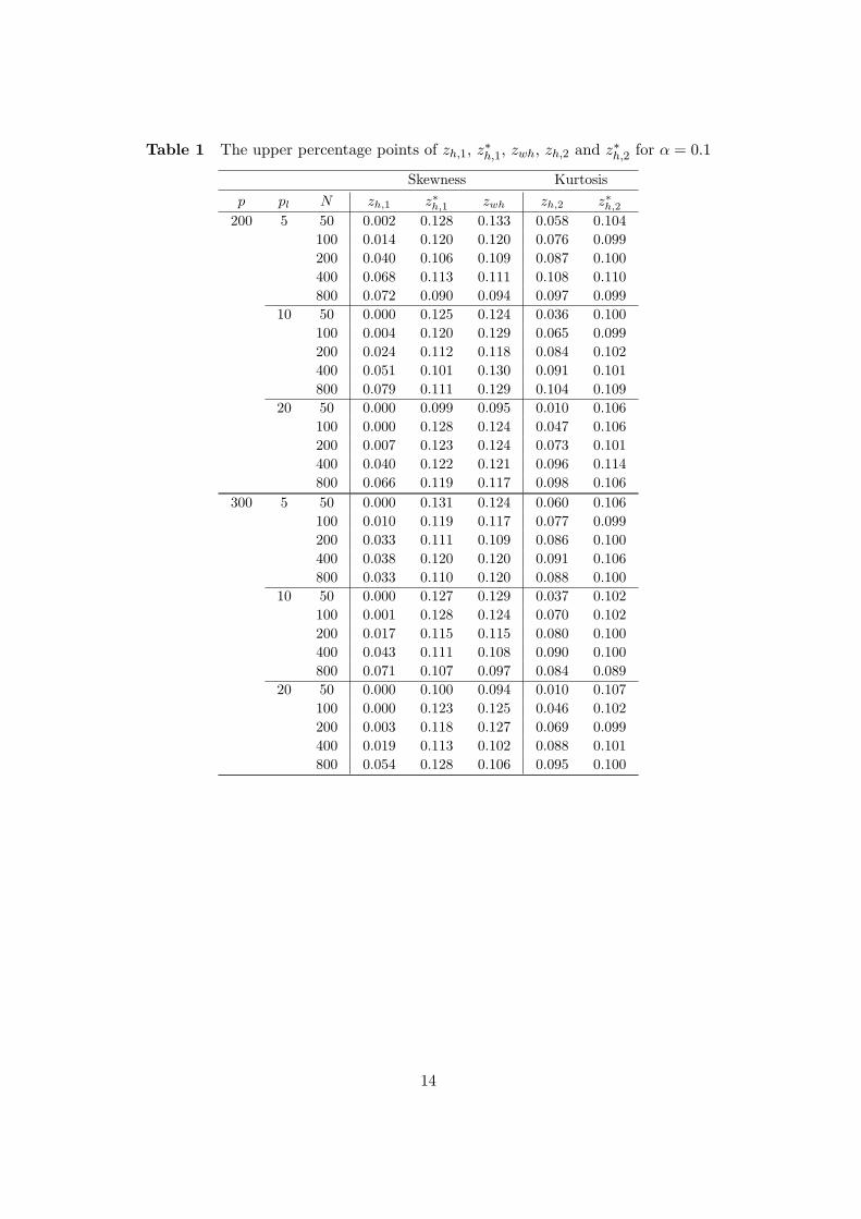
Table 1 The upper percentage points of zh,1, z∗h,1, zwh, zh,2 and z∗h,2 for α = 0.1
Skewness Kurtosis
p pl N zh,1 z∗h,1 zwh zh,2 z∗h,2200 5 50 0.002 0.128 0.133 0.058 0.104
100 0.014 0.120 0.120 0.076 0.099
200 0.040 0.106 0.109 0.087 0.100
400 0.068 0.113 0.111 0.108 0.110
800 0.072 0.090 0.094 0.097 0.099
10 50 0.000 0.125 0.124 0.036 0.100
100 0.004 0.120 0.129 0.065 0.099
200 0.024 0.112 0.118 0.084 0.102
400 0.051 0.101 0.130 0.091 0.101
800 0.079 0.111 0.129 0.104 0.109
20 50 0.000 0.099 0.095 0.010 0.106
100 0.000 0.128 0.124 0.047 0.106
200 0.007 0.123 0.124 0.073 0.101
400 0.040 0.122 0.121 0.096 0.114
800 0.066 0.119 0.117 0.098 0.106
300 5 50 0.000 0.131 0.124 0.060 0.106
100 0.010 0.119 0.117 0.077 0.099
200 0.033 0.111 0.109 0.086 0.100
400 0.038 0.120 0.120 0.091 0.106
800 0.033 0.110 0.120 0.088 0.100
10 50 0.000 0.127 0.129 0.037 0.102
100 0.001 0.128 0.124 0.070 0.102
200 0.017 0.115 0.115 0.080 0.100
400 0.043 0.111 0.108 0.090 0.100
800 0.071 0.107 0.097 0.084 0.089
20 50 0.000 0.100 0.094 0.010 0.107
100 0.000 0.123 0.125 0.046 0.102
200 0.003 0.118 0.127 0.069 0.099
400 0.019 0.113 0.102 0.088 0.101
800 0.054 0.128 0.106 0.095 0.100
14
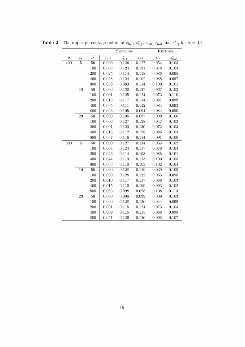
Table 2 The upper percentage points of zh,1, z∗h,1, zwh, zh,2 and z∗h,2 for α = 0.1
Skewness Kurtosis
p pl N zh,1 z∗h,1 zwh zh,2 z∗h,2400 5 50 0.000 0.126 0.127 0.054 0.103
100 0.006 0.124 0.121 0.078 0.103
200 0.025 0.114 0.118 0.086 0.098
400 0.058 0.124 0.102 0.088 0.097
800 0.058 0.083 0.114 0.100 0.101
10 50 0.000 0.130 0.127 0.037 0.102
100 0.001 0.125 0.124 0.073 0.110
200 0.013 0.117 0.114 0.081 0.099
400 0.035 0.111 0.112 0.084 0.093
800 0.063 0.105 0.094 0.084 0.090
20 50 0.000 0.105 0.097 0.009 0.106
100 0.000 0.127 0.128 0.047 0.102
200 0.001 0.123 0.130 0.072 0.103
400 0.016 0.112 0.128 0.086 0.103
800 0.037 0.116 0.114 0.091 0.100
500 5 50 0.000 0.127 0.134 0.055 0.102
100 0.004 0.124 0.117 0.076 0.104
200 0.023 0.114 0.108 0.088 0.101
400 0.044 0.113 0.113 0.100 0.105
800 0.063 0.110 0.103 0.102 0.104
10 50 0.000 0.128 0.119 0.039 0.109
100 0.000 0.128 0.122 0.063 0.098
200 0.010 0.117 0.117 0.086 0.103
400 0.015 0.110 0.109 0.093 0.102
800 0.053 0.098 0.098 0.108 0.113
20 50 0.000 0.098 0.099 0.009 0.103
100 0.000 0.128 0.126 0.044 0.099
200 0.001 0.115 0.124 0.073 0.103
400 0.009 0.115 0.115 0.088 0.098
800 0.051 0.126 0.126 0.098 0.107
15

Table 3 The upper percentage points of zh,1, z∗h,1, zwh, zh,2 and z∗h,2 for α = 0.05
Skewness Kurtosis
p pl N zh,1 z∗h,1 zwh zh,2 z∗h,2200 5 50 0.000 0.072 0.072 0.021 0.055
100 0.006 0.063 0.068 0.033 0.050
200 0.018 0.056 0.056 0.043 0.052
400 0.029 0.060 0.054 0.055 0.060
800 0.038 0.047 0.044 0.049 0.051
10 50 0.000 0.070 0.071 0.011 0.053
100 0.001 0.063 0.072 0.026 0.049
200 0.009 0.063 0.063 0.039 0.052
400 0.029 0.058 0.080 0.041 0.045
800 0.040 0.061 0.056 0.056 0.059
20 50 0.000 0.050 0.048 0.002 0.055
100 0.000 0.074 0.071 0.017 0.053
200 0.002 0.068 0.073 0.031 0.052
400 0.016 0.067 0.066 0.044 0.058
800 0.031 0.066 0.058 0.048 0.056
300 5 50 0.000 0.076 0.072 0.023 0.057
100 0.004 0.066 0.065 0.034 0.052
200 0.015 0.060 0.060 0.043 0.052
400 0.017 0.064 0.058 0.043 0.054
800 0.014 0.057 0.058 0.042 0.051
10 50 0.000 0.076 0.075 0.011 0.054
100 0.000 0.073 0.068 0.031 0.054
200 0.007 0.064 0.062 0.036 0.048
400 0.022 0.057 0.055 0.040 0.048
800 0.028 0.056 0.055 0.039 0.044
20 50 0.000 0.053 0.049 0.001 0.054
100 0.000 0.071 0.071 0.017 0.053
200 0.001 0.064 0.071 0.029 0.049
400 0.008 0.060 0.065 0.040 0.051
800 0.027 0.068 0.049 0.050 0.055
16
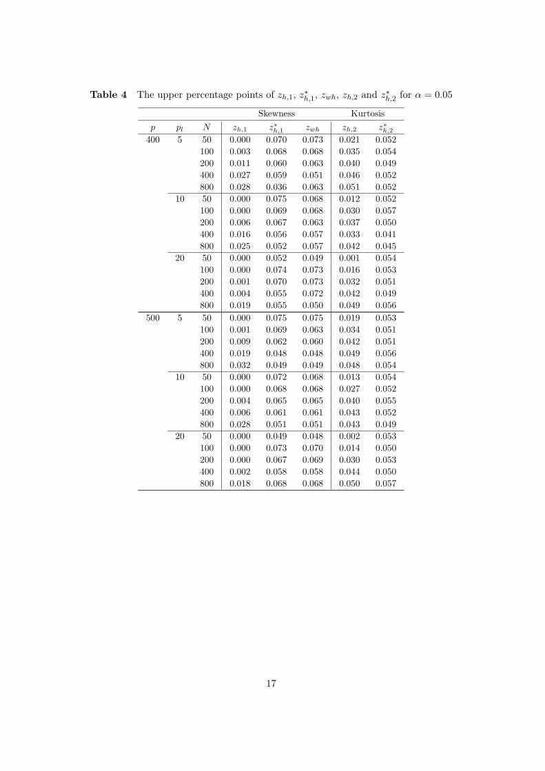
Table 4 The upper percentage points of zh,1, z∗h,1, zwh, zh,2 and z∗h,2 for α = 0.05
Skewness Kurtosis
p pl N zh,1 z∗h,1 zwh zh,2 z∗h,2400 5 50 0.000 0.070 0.073 0.021 0.052
100 0.003 0.068 0.068 0.035 0.054
200 0.011 0.060 0.063 0.040 0.049
400 0.027 0.059 0.051 0.046 0.052
800 0.028 0.036 0.063 0.051 0.052
10 50 0.000 0.075 0.068 0.012 0.052
100 0.000 0.069 0.068 0.030 0.057
200 0.006 0.067 0.063 0.037 0.050
400 0.016 0.056 0.057 0.033 0.041
800 0.025 0.052 0.057 0.042 0.045
20 50 0.000 0.052 0.049 0.001 0.054
100 0.000 0.074 0.073 0.016 0.053
200 0.001 0.070 0.073 0.032 0.051
400 0.004 0.055 0.072 0.042 0.049
800 0.019 0.055 0.050 0.049 0.056
500 5 50 0.000 0.075 0.075 0.019 0.053
100 0.001 0.069 0.063 0.034 0.051
200 0.009 0.062 0.060 0.042 0.051
400 0.019 0.048 0.048 0.049 0.056
800 0.032 0.049 0.049 0.048 0.054
10 50 0.000 0.072 0.068 0.013 0.054
100 0.000 0.068 0.068 0.027 0.052
200 0.004 0.065 0.065 0.040 0.055
400 0.006 0.061 0.061 0.043 0.052
800 0.028 0.051 0.051 0.043 0.049
20 50 0.000 0.049 0.048 0.002 0.053
100 0.000 0.073 0.070 0.014 0.050
200 0.000 0.067 0.069 0.030 0.053
400 0.002 0.058 0.058 0.044 0.050
800 0.018 0.068 0.068 0.050 0.057
17

Table 5 The upper percentage points of zh,1, z∗h,1, zwh, zh,2 and z∗h,2 for α = 0.01
Skewness Kurtosis
p pl N zh,1 z∗h,1 zwh zh,2 z∗h,2200 5 50 0.000 0.020 0.018 0.002 0.011
100 0.001 0.015 0.018 0.006 0.012
200 0.003 0.013 0.013 0.007 0.011
400 0.004 0.008 0.014 0.010 0.011
800 0.008 0.014 0.011 0.009 0.010
10 50 0.000 0.018 0.021 0.001 0.012
100 0.000 0.017 0.020 0.003 0.010
200 0.001 0.014 0.014 0.006 0.012
400 0.008 0.020 0.015 0.007 0.011
800 0.006 0.009 0.015 0.014 0.017
20 50 0.000 0.010 0.010 0.000 0.012
100 0.000 0.019 0.018 0.001 0.012
200 0.000 0.016 0.018 0.004 0.010
400 0.002 0.016 0.015 0.010 0.010
800 0.005 0.014 0.012 0.010 0.011
300 5 50 0.000 0.021 0.021 0.002 0.013
100 0.001 0.017 0.017 0.004 0.011
200 0.002 0.014 0.016 0.008 0.012
400 0.003 0.016 0.010 0.008 0.011
800 0.003 0.013 0.016 0.009 0.013
10 50 0.000 0.019 0.020 0.001 0.011
100 0.000 0.019 0.020 0.003 0.013
200 0.001 0.016 0.015 0.006 0.010
400 0.004 0.015 0.014 0.008 0.010
800 0.003 0.007 0.017 0.011 0.012
20 50 0.000 0.010 0.009 0.000 0.013
100 0.000 0.021 0.018 0.002 0.012
200 0.001 0.014 0.019 0.004 0.009
400 0.001 0.013 0.018 0.006 0.010
800 0.007 0.017 0.012 0.009 0.010
18

Table 6 The upper percentage points of zh,1, z∗h,1, zwh, zh,2 and z∗h,2 for α = 0.01
Skewness Kurtosis
p pl N zh,1 z∗h,1 zwh zh,2 z∗h,2400 5 50 0.000 0.020 0.019 0.003 0.013
100 0.000 0.018 0.019 0.005 0.011
200 0.002 0.013 0.016 0.007 0.010
400 0.005 0.012 0.010 0.008 0.009
800 0.007 0.010 0.012 0.008 0.009
10 50 0.000 0.020 0.019 0.001 0.013
100 0.000 0.019 0.018 0.004 0.013
200 0.001 0.019 0.014 0.007 0.010
400 0.003 0.013 0.012 0.006 0.012
800 0.002 0.011 0.010 0.004 0.005
20 50 0.000 0.008 0.010 0.000 0.012
100 0.000 0.020 0.020 0.001 0.011
200 0.000 0.018 0.019 0.004 0.011
400 0.001 0.016 0.020 0.008 0.012
800 0.001 0.010 0.009 0.009 0.010
500 5 50 0.000 0.021 0.019 0.002 0.011
100 0.000 0.019 0.016 0.005 0.010
200 0.002 0.014 0.013 0.008 0.010
400 0.004 0.007 0.007 0.008 0.009
800 0.005 0.009 0.010 0.008 0.009
10 50 0.000 0.019 0.018 0.001 0.013
100 0.000 0.018 0.018 0.003 0.012
200 0.000 0.018 0.018 0.007 0.011
400 0.000 0.012 0.012 0.003 0.008
800 0.006 0.010 0.010 0.004 0.005
20 50 0.000 0.009 0.008 0.000 0.012
100 0.000 0.019 0.019 0.001 0.010
200 0.000 0.018 0.017 0.005 0.012
400 0.000 0.011 0.011 0.006 0.013
800 0.004 0.015 0.015 0.009 0.012
19
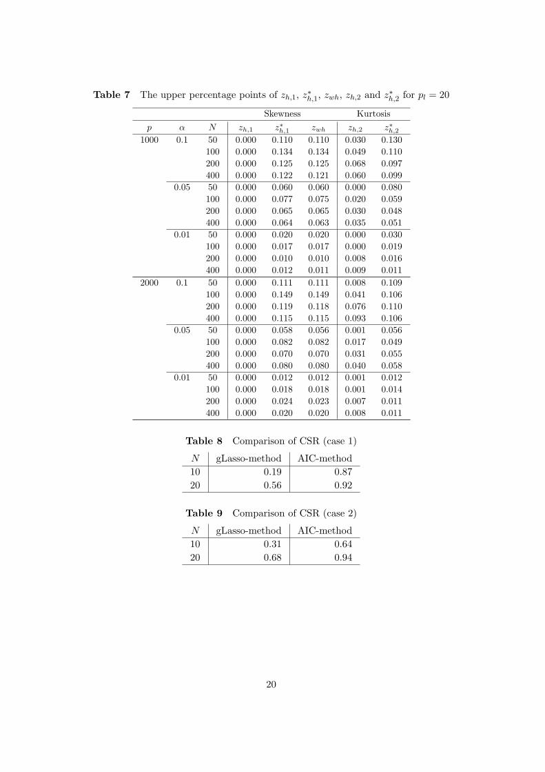
Table 7 The upper percentage points of zh,1, z∗h,1, zwh, zh,2 and z∗h,2 for pl = 20
Skewness Kurtosis
p α N zh,1 z∗h,1 zwh zh,2 z∗h,21000 0.1 50 0.000 0.110 0.110 0.030 0.130
100 0.000 0.134 0.134 0.049 0.110
200 0.000 0.125 0.125 0.068 0.097
400 0.000 0.122 0.121 0.060 0.099
0.05 50 0.000 0.060 0.060 0.000 0.080
100 0.000 0.077 0.075 0.020 0.059
200 0.000 0.065 0.065 0.030 0.048
400 0.000 0.064 0.063 0.035 0.051
0.01 50 0.000 0.020 0.020 0.000 0.030
100 0.000 0.017 0.017 0.000 0.019
200 0.000 0.010 0.010 0.008 0.016
400 0.000 0.012 0.011 0.009 0.011
2000 0.1 50 0.000 0.111 0.111 0.008 0.109
100 0.000 0.149 0.149 0.041 0.106
200 0.000 0.119 0.118 0.076 0.110
400 0.000 0.115 0.115 0.093 0.106
0.05 50 0.000 0.058 0.056 0.001 0.056
100 0.000 0.082 0.082 0.017 0.049
200 0.000 0.070 0.070 0.031 0.055
400 0.000 0.080 0.080 0.040 0.058
0.01 50 0.000 0.012 0.012 0.001 0.012
100 0.000 0.018 0.018 0.001 0.014
200 0.000 0.024 0.023 0.007 0.011
400 0.000 0.020 0.020 0.008 0.011
Table 8 Comparison of CSR (case 1)
N gLasso-method AIC-method
10 0.19 0.87
20 0.56 0.92
Table 9 Comparison of CSR (case 2)
N gLasso-method AIC-method
10 0.31 0.64
20 0.68 0.94
20
References
[1] Akaike, H. (1973). Information theory and an extension of the maximum likelihood princi-ple. Second International Symposium on Information Theory, 1, 267–281.
[2] Akaike, H. (1974). A new look at the statistical model identification. IEEE Transactionson Automatic Control, 19, 716–723.
[3] Cramer, H. (1946). Mathematical Methods of Statistics. Princeton University Press.
[4] Enomoto, R., Okamoto, N. and Seo, T. (2012). Multivariate normality test using Srivas-tava’s skewness and kurtosis. SUT Journal of Mathematics, 48, 103–115.
[5] Friedman, J., Hastie, T. and Tibshirani, R. (2008). Sparse inverse covariance estimationwith the graphical lasso. Biostatistics, 9, 432–441.
[6] Henze, N. (2002). Invariant tests for multivariate normality: a critical review. StatisticalPapers, 43, 467–506.
[7] Khatri, C. G. (1959). On the mutual independence of certain statistics. Annals of Mathe-matical Statistics, 30, 1258–1262.
[8] Khatri, C. G. and Pillai, K. C. S. (1967). On the moments of traces of two matrices inmultivariate analysis. Annals of the Institute of Statistical Mathematics, 19, 143–156.
[9] Koizumi, K., Hyodo, M. and Pavlenko, T. (2013). Modified Jarque-Bera type tests formultivariate normality in a high-dimensional framework. (submitted).
[10] Kullback, S. and Leibler, R. (1951). On information and sufficiency. The Annals of Mathe-matical Statistics, 22, 79–86.
[11] Malkovich, J. F. and Afifi, A. A. (1973). On tests for multivariate normality. Journal of theAmerican Statistical Association, 68, 176–179.
[12] Mardia, K. V. (1970). Measures of multivariate skewness and kurtosis with applications.Biometrika, 57, 519–530.
[13] Mardia, K. V. (1974). Applications of some measures of multivariate skewness and kurtosisin testing normality and robustness studies. Sankhya B, 36, 115–128.
[14] Miyagawa, C., Koizumi, K. and Seo, T. (2011). A new multivariate kurtosis and its asymp-totic distribution. SUT Journal of Mathematics, 47, 55–71.
[15] Pavlenko, T., Bjorkstrom, A. and Tillander, A. (2012). Covariance structure approximationvia gLasso in high-dimensional supervised classification. Journal of Applied Statistics, 39,1643–1666.
[16] Rao, C. R. (1965). Linear Statistical Inference and its Applications. Wiley, New York.
[17] Rothman,.A., Bickel, P., Levina, E. and Zhu, J. (2008). Sparse permutation invariant co-variance estimation. Electronic Journal of Statistics, 2, 494–515.
21

[18] Rutimann,.P. and Buhlmann,.P. (2009). High dimensional sparse covariance estimation viadirected acyclic graphs. Electronic Journal of Statistics, 3, 1133–1160.
[19] Srivastava, M. S. (1984). A measure of skewness and kurtosis and a graphical method forassessing multivariate normality. Statistics & Probability Letters, 2, 263–267.
[20] Thode, H. C. (2002). Testing for normality. Marcel Dekker.
[21] Wilson, E. B. and Hilferty, M. M. (1931). The distribution of chi-square. Mathematics, 17,684–688.
22