Measures of central tendency - University of Notre Damedgalvin1/10120/10120_S17/Topic15_8p...Measures of central tendency A sample is a subset of the population, for example, we might

Measures of central tendency

Questions such as: “how many calories do I eat per day?”or “how much time do I spend talking per day?” can behard to answer because the answer will vary from day today. It’s sometimes more sensible to ask “how manycalories do I consume on a typical day?” or “on average,how much time do I spend talking per day?”.

In this section we will study three ways of measuringcentral tendency in data, the mean, the median and themode. Each measure give us a single value? that might beconsidered typical. Each measure has its own strengths andweaknesses

?: some exclusions apply


A population of books, cars, people, polar bears, all gamesplayed by Babe Ruth throughout his career, etc., is theentire collection of those objects. For any given variableunder consideration, each member of the population has aparticular value of the variable associated to them, forexample the number of home runs scored by Babe Ruth foreach game played by him during his career. These valuesare called data and we can apply our measures of centraltendency to the entire population, to get a single value(maybe more than one for the mode) measuring centraltendency for the entire population; or we can apply ourmeasures to a subset or sample of the population, to get anestimate of the central tendency for the population.


A sample is a subset of the population, for example, wemight collect data on the number of home runs hit byMiguel Cabrera in a random sample of 20 games. If wecalculate the mean, median and mode using the data froma sample, the results are called the sample mean, samplemedian and sample mode.

Sometimes we can look at the entire population, not just asubset. For example, since Babe Ruth has now retired, sowe might collect data on the number of home runs he hit inhis career. If we calculate the mean, median and modeusing the data collected from the entire population, theresults are called the population mean, population medianand population mode.

Mean

The population mean of m numbers x1, x2, . . . , xm (thedata for every member of a population of size m) is denotedby µ and is computed as follows:

µ =x1 + x2 + · · · + xm

m.

The sample mean of the numbers x1, x2, . . . , xn (data fora sample of size n from the population) is denoted by x̄ andis computed similarly:

x̄ =x1 + x2 + · · · + xn

n.

Mean

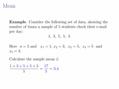
Example Consider the following set of data, showing thenumber of times a sample of 5 students check their e-mailper day:

1, 3, 5, 5, 3.

Here n = 5 and x1 = 1, x2 = 3, x3 = 5, x4 = 5 andx5 = 3.

Calculate the sample mean x̄.

1 + 3 + 5 + 5 + 3

5=

17

5= 3.4

Mean

Example The following data shows the results for thenumber of books that a random sample of 20 students werecarrying in their book bags:

0, 1, 1, 2, 2, 2, 2, 2, 2, 2, 2, 3, 3, 3, 3, 4, 4, 4, 4, 4

Then the mean of the sample is the average number ofbooks carried per student:

x̄ =0 + 1 + 1 + 2 + 2 + 2 + 2 + 2 + 2 + 2 + 2 + 3 + 3 + 3 + 3 + 4 + 4 + 4 + 4 + 4

20= 2.5

Note that the mean does not necessarily have to be one ofthe values observed in our data; in this case it is a valuethat could never be observed.

Calculating the mean more efficientlyWe can calculate the mean above more efficiently here byusing frequencies. We can see from the calculation abovethat

x̄ =0 + (1 × 2) + (2 × 8) + (3 × 4) + (4 × 5)

20= 2.5

The frequency distribution for the data is:

# Books Frequency # Books ×Frequency

0 1 0 × 1

1 2 1 × 2

2 8 2 × 8

3 4 3 × 4

4 5 4 × 5

x̄ = Sum20

= 5020

= 2.5

Calculating the mean more efficiently

In general: If the frequency/relative frequency table for oursample of size n looks like the one below (where theobservations are denoted Oi, the corresponding frequenciesby fi and the relative frequencies by fi/n):

Observation Frequency Relative FrequencyOi fi fi/nO1 f1 f1/nO2 f2 f2/nO3 f3 f3/n...

......

OR fR fR/n

then:


x̄ =O1 · f1 +O2 · f2 + · · · +OR · fR

n=

O1 ·f1n

+O2 ·f2n

+O3 ·f3n

+ · · ·OR · fRn

We can also use our table with a new column to calculate:Outcome Frequency Outcome × Frequency

Oi fi Oi × fiO1 f1 O1 × f1O2 f2 O2 × f2O3 f3 O3 × f3...

......

OR .fR OR × fR

SUM

n= x̄


Alternatively we can use the relative frequencies, instead ofdividing by the n at the end.

Outcome Frequency Relative Frequency Outcome × Relative FrequencyOi fi fi/n Oi × fi/nO1 f1 f1/n O1 × f1/nO2 f2 f2/n O2 × f2/nO3 f3 f3/n O3 × f3/n...

......

...OR .fR fR/n OR × fR/n

SUM = x̄

You can of course choose any method for calculation fromthe three methods listed above. The easiest method to usewill depend on how the data is presented.

Calculating the mean more efficientlyExample The number of goals scored by the 32 teams inthe 2014 world cup are shown below:

18, 15, 12, 11, 10, 8, 7, 7, 6, 6, 6, 5, 5, 5, 4,

4, 4, 4, 4, 4, 3, 3, 3, 3, 3, 2, 2, 2, 2, 1, 1, 1

Make a frequency table for the data and, taking the soccerteams who played in the world cup as a population,calculate the population mean, µ.

Outcome Frequency1 32 43 54 65 36 37 2

Outcome Frequency8 110 111 112 115 118 1µ = ?


Outcome Frequency1 32 43 54 65 36 37 2

Outcome Frequency8 110 111 112 115 118 1µ = 5.34375

µ =1 · 3 + 2 · 4 + 3 · 5 + 4 · 6 + 5 · 3 + 6 · 3 + 7 · 2 + 8 · 1 + 10 · 1 + 11 · 1 + 12 · 1 + 15 · 1 + 18 · 1

32

=3 + 8 + 15 + 24 + 15 + 18 + 14 + 8 + 10 + 11 + 12 + 15 + 18

32=

171

32= 5.34375

Estimating the mean from a histogram

If we are given a histogram (showing frequencies) or afrequency table where the data is already grouped intocategories, and we do not have access to the original data,we can still estimate the mean using the midpoints of theintervals which serve as categories for the data. Supposethere are k categories (shown as the bases of the rectangles)with midpoints m1,m2, . . . ,mk respectively and thefrequencies of the corresponding intervals are f1, f2, . . . , fk,then the mean of the data set is approximately

m1f1 +m2f2 + · · · +mkfkn

where n = f1 + f2 + · · · + fk.

Estimating the mean from a histogramExample Approximate the mean for the set of data usedto make the following histogram, showing the time (inseconds) spent waiting by a sample of customers atGringotts Wizarding bank.

250-300 300-350

2

4

6

8

10

12

50-100 100-150 150-200 200-250

Time spent waiting (in seconds)

midpoints:

approximation of samplemean:


midpoints:50 + 100

2= 75

100 + 150

2= 125

150 + 200

2= 175

200 + 250

2= 225

250 + 300

2= 275

300 + 350

2= 325

Outcome Frequency75 12125 10175 4225 2275 1325 1

Sample size 30


x̄approx =75 · 12 + 125 · 10 + 175 · 4 + 225 · 2 + 275 · 1 + 325 · 1

30

=900 + 1250 + 700 + 450 + 275 + 325

30=

3900

30= 130

This calculation only gives an approximation to the samplemean because I do not know the distribution of actual waittimes within each bar (cf. the two histograms for OldFaithful eruption durations in the previous section’s slides).


We can calculate the minimum possible sample mean byassuming all the people in each bar are at the left handedge. For example, all 12 people in the first bar waited 50seconds. This gives a result of x̄min = 105.

We can also calculate the maximal possible sample meanby assuming all the people in each bar are at the right handedge. This gives the result x̄max = 155.

Notice

x̄approx =x̄min + x̄max

2

and the actual sample mean, x̄ satisfies the inequalities

x̄min 6 x̄ 6 x̄max

The Median

The Median of a set of quantitative data is the middlenumber when the measurements are arranged in ascendingorder.

To Calculate the Median: Arrange the nmeasurements in ascending (or descending) order. Wedenote the median of the data by M.

1. If n is odd, M is the middle number.

2.If n is even, M is the average of the two middle numbers.

The MedianExample The number of goals scored by the 32 teams inthe 2014 world cup are shown below:

18, 15, 12, 11, 10, 8, 7, 7, 6, 6, 6, 5, 5, 5, 4,

4, 4, 4, 4, 4, 3, 3, 3, 3, 3, 2, 2, 2, 2, 1, 1, 1

Find the median of the above set of data.

The data is in descending order. There are 32 events andhalf of 32 is 16. Sixteen elements from the right is 4,indicated in green in the list below. Sixteen elements fromthe left is 4, indicated in red in the list below. The median

is 4 =4 + 4

2.

18, 15, 12, 11, 10, 8, 7, 7, 6, 6, 6, 5, 5, 5, 4, 4,

4, 4, 4, 4, 3, 3, 3, 3, 3, 2, 2, 2, 2, 1, 1, 1,

The Median

Example A sample of 5 students were asked how muchmoney they were carrying and the results are shown below:

$75, $2, $5, $0, $5.

Find the mean and median of the above set of data.

The data in ascending order is 0, 2, 5, 5, 75. The median is0 + 2 + 5 + 5 + 75

5=

87

5= 17.4. There are 5 = 2 · 3 − 1

numbers so to find the median count in 3 from either endto get 5.

Notice that the median gives us a more representativepicture here, since the mean is skewed by the outlier $75.

The Mode

The mode of a set of measurements is the most frequentlyoccurring value; it is the value having the highest frequencyamong the measurements.

Example Find the mode of the data collected on theamount of money carried by the 5 students in the exampleabove:

$75, $2, $5, $0, $5.

Since 5 occurs twice and all the other events are unique,the mode is 5.

The Mode

Example What is the mode of the data on the number ofgoals scored by each team in the world cup of 2006?

18, 15, 12, 11, 10, 8, 7, 7, 6, 6, 6, 5, 5, 5, 4,

4, 4, 4, 4, 4, 3, 3, 3, 3, 3, 2, 2, 2, 2, 1, 1, 1

Here is the frequency table:18 17 16 15 14 13 12 11 10 9 8 7 6 5 4 3 2 11 0 0 1 0 0 1 1 1 0 1 2 3 3 6 5 4 3

To find the mode, look in the frequency table for thelargest number(s) there. In this case 4 occurs 6 times andno other entry occurs this many times so the mode is 4.

The Mode

Notes 1) The mode need not be unique: if over the courseof a week I drink 3,2,2,3,4,1,1 cups of coffee per day, themode number of cups I drink is 1, and 2, and 3.

The mode can be computed for qualitative data. Forexample, if in this class we have 11 people with blue eyes, 6with green eyes, 5 with hazel eyes, 4 with brown eyes and 1with purple eyes, then the mode eye color is blue, but itmakes no sense to talk about the mean or median eyecolour.

The Histogram and the mean, median and mode

With large sets of data and narrow class widths, thehistogram looks roughly like a smooth curve. The mean,median and mode, have a graphical interpretation in thiscase.

I The mean is the balance point of the histogram of thedata (the point on the horizontal axis from where Iwould pick up the histogram to balance it on myfinger)

I the median is the point on the horizontal axis suchthat half of the area under the histogram lies to theright of the median and half of the area lies to its left.

I The mode occurs at the data point where the graphreaches its highest point (maybe not unique).

The Histogram and the mean, median and mode

5.2.4 Which Measure of Center to Use?

Bell-shaped, Symmetric Bimodal

mean=median=mode

50%

mean=median

two modes

Skewed Right Skewed Left

mode

median

mean

50%

mode

median

mean

50%

Mean, Median, and Mode

The most common measure of center is the mean, which locates the

balancing point of the distribution. The mean equals the sum of the

observations, divided by how many there are. The mean is also affected by

extreme observations (outliers and values which are far in the tail of a

distribution that is skewed). So the mean tends to be a good choice for

locating the center of a distribution that is unimodal and roughly symmetric,

with no outliers.

The median is a more robust measure of center, that is, it is not influenced

by extreme values. The median is the middle observation when the data are

p. 315



mean=median=mode

50%

mean=median

two modes


mode

median

mean

50%

mode

median

mean

50%








with no outliers.



p. 315



mean=median=mode

50%

mean=median

two modes


mode

median

mean

50%

mode

median

mean

50%








with no outliers.



p. 315

Skewed Left

For data skewed to the right, the mean is larger than the

median, and for data skewed to left, the mean is less than the

median.

Skewed DataA data set is said to be skewed if one tail of thedistribution has more extreme observations than the othertail. The mean is sensitive to extreme observations, but themedian is not.

Consider the previous example with data on the amount ofmoney carried by a sample of five students:

$75, $2, $5, $0, $5.

We have already calculated mean = $17.4, median = $5.

Now consider the same set of data with the largest amountof money replaced by $5,000:

$5, 000, $2, $5, $0, $5.

What is the new mean and median? The median is thesame, 5 but the mean is (5000 + 2 + 5 + 0 + 5)/5 = 1002.4

Comparing different measures

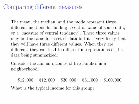
The mean, the median, and the mode represent threedifferent methods for finding a central value of some data,or a “measure of central tendancy”. These three valuesmay be the same for a set of data but it is very likely thatthey will have three different values. When they aredifferent, they can lead to different interpretations of thedata being summarized.

Consider the annual incomes of five families in aneighborhood:

$12, 000 $12, 000 $30, 000 $51, 000 $100, 000

What is the typical income for this group?

Comparing different measures

$12, 000 $12, 000 $30, 000 $51, 000 $100, 000

I The mean income is: $41,000,

I The median income is: $30,000,

I The mode income is: $12,000.

If you were trying to promote that this is an affluentneighborhood, you might prefer to report the mean income.

If you were a Sociologist, trying to report a typical incomefor the area, you might report the median income.

If you were trying to argue against a property tax increase,you might argue that income is too low to afford a taxincrease and report the mode.

Documents

Measures of central tendency - University of Notre Damedgalvin1/10120/10120_S17/Topic15_8p...Measures of central tendency A sample is a subset of the population, for example, we might