Measures of Central Tendency Purpose is to describe a distribution’s

typical case – do not say “average” case Mode Median Mean (Average)

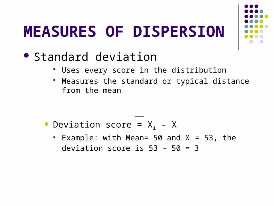
MEASURES OF DISPERSION

Standard deviation Uses every score in the distribution Measures the standard or typical distance from the

mean

Deviation score = Xi - X Example: with Mean= 50 and Xi = 53, the deviation

score is 53 - 50 = 3

X Xi - X8 +5 1 -23 00 -312 0

Mean = 3 •Deviation scoresadd up to zero

•Because sum of deviationsis always 0, it can’t be used as a measure of dispersion

The Problem with Summing Deviations From Mean• 2 parts to a deviation score: the sign and the number

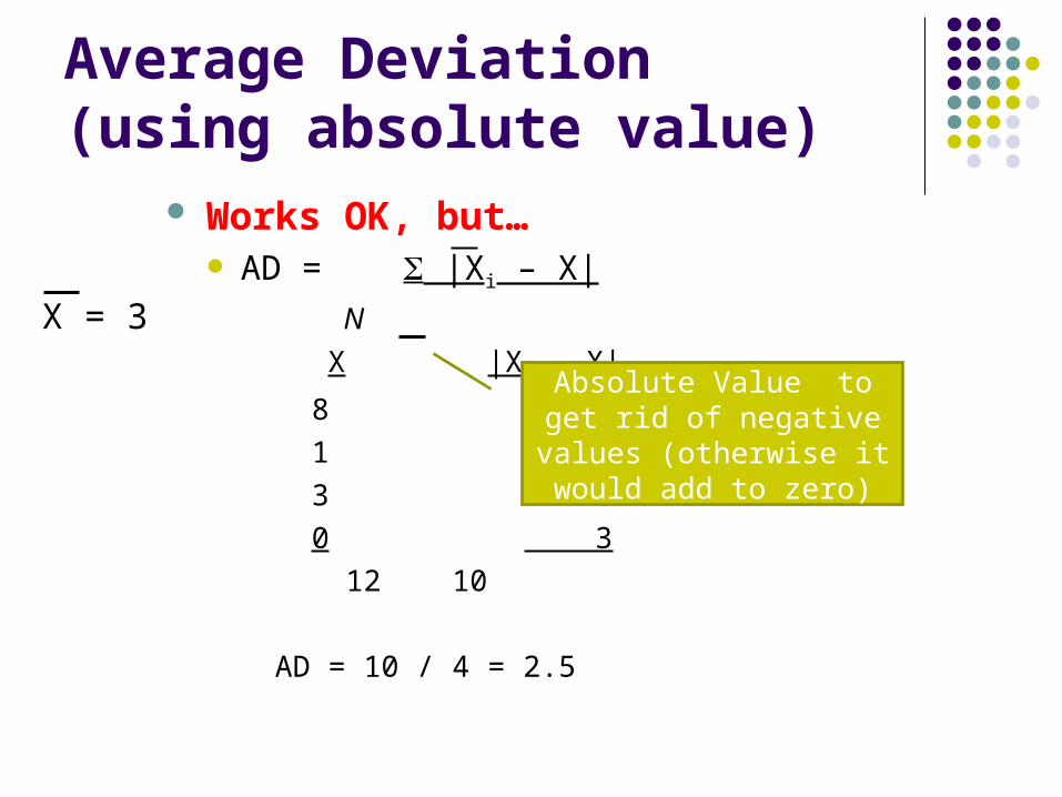
Average Deviation (using absolute value)

Works OK, but… AD = |Xi – X|

N

X |Xi – X|

8 5

1 2

3 0

0 3

12 10

AD = 10 / 4 = 2.5

X = 3

Absolute Value to get rid of negative values

(otherwise it would add to zero)

Variance & Standard Deviation

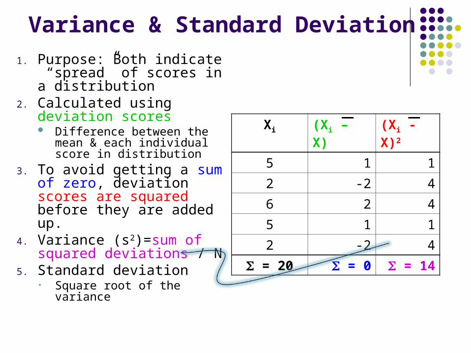
1. Purpose: Both indicate “spread” of scores in a distribution

2. Calculated using deviation scores Difference between the

mean & each individual score in distribution

3. To avoid getting a sum of zero, deviation scores are squared before they are added up.

4. Variance (s2)=sum of squared deviations / N

5. Standard deviation• Square root of the variance

Xi (Xi – X) (Xi - X)2

5 1 1

2 -2 4

6 2 4

5 1 1

2 -2 4

= 20 = 0 = 14

Terminology

“Sum of Squares” = Sum of Squared Deviations from the Mean = (Xi - X)2

Variance = sum of squares divided by sample size = (Xi - X)2 = s2

N Standard Deviation = the square root of the

variance = s

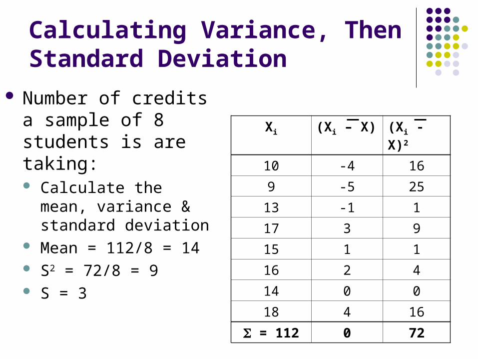
Calculating Variance, Then Standard Deviation

Number of credits a sample of 8 students is are taking: Calculate the mean,

variance & standard deviation

Mean = 112/8 = 14 S2 = 72/8 = 9 S = 3

Xi (Xi – X) (Xi - X)2

10 -4 16

9 -5 25

13 -1 1

17 3 9

15 1 1

16 2 4

14 0 0

18 4 16

= 112 0 72

Summary Points about the Standard Deviation

1. Uses all the scores in the distribution

2. Provides a measure of the typical, or standard, distance from the mean

Increases in value as the distribution becomes more heterogeneous

3. Useful for making comparisons of variation between distributions

4. Becomes very important when we discuss the normal curve (Chapter 5, next)

Mean & Standard Deviation Together

Tell us a lot about the typical score & how the scores spread around that score Useful for comparisons of distributions: Example:

Class A: mean GPA 2.8, s = 0.3 Class B: mean GPA 3.3, s = 0.6 Mean & Standard Deviation Applet

Example Using SPSS Output

Hours watching TV for Soc 3155 students:

1. What is the range & interquartile range?

2. Is there skew (positive or negative) in this distribution?

3. What is the most common number of hours reported?

4. What is the average squared distance that cases deviate from the mean?

StatisticsHours watch TV in typical weekN Valid 18 Missing 11

Mean 8.2778Median 5.0000Mode 5.00Std. Deviation 7.97648Variance 63.624Minimum 1.00Maximum 28.00Percentiles

25 3.000050 5.000075 14.0000

The Normal Curve & Z Scores

THE NORMAL CURVE Characteristics:

Theoretical distribution of scores

Perfectly symmetrical Bell-shaped Unimodal Continuous

There is a value of Y for every value of X, where X is assumed to be continuous variable

Tails extend infinitely in both directions

x AXIS

Y

axis

THE NORMAL CURVE

Assumption of normality of a given empirical distribution makes it possible to describe this “real-world” distribution based on what we know about the (theoretical) normal curve

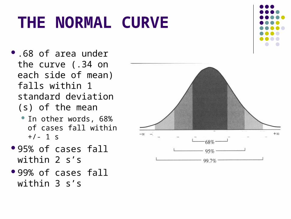
THE NORMAL CURVE

.68 of area under the curve (.34 on each side of mean) falls within 1 standard deviation (s) of the mean In other words, 68% of

cases fall within +/- 1 s

95% of cases fall within 2 s’s

99% of cases fall within 3 s’s

Areas Under the Normal Curve

Because the normal curve is symmetrical, we know that 50% of its area falls on either side of the mean.

FOR EACH SIDE: 34.13% of scores in

distribution are b/t the mean and 1 s from the mean

13.59% of scores are between 1 and 2 s’s from the mean

2.28% of scores are > 2 s’s from the mean

THE NORMAL CURVE Example:

Male height = normally distributed, mean = 70 inches, s = 4 inches

What is the range of heights that encompasses 99% of the population?

Hint: that’s +/- 3 standard deviations

Answer: 70 +/- (3)(4) = 70 +/- 12

Range = 58 to 82

THE NORMAL CURVE & Z SCORES

– To use the normal curve to answer questions, raw scores of a distribution must be transformed into Z scores

• Z scores:

Formula: Zi = Xi – X

s– A tool to help

determine how a given score measures up to the whole distribution

RAW SCORES: 66 70 74Z SCORES: -1 0 1

NORMAL CURVE & Z SCORES Transforming raw scores to

Z scores a.k.a. “standardizing” converts all values of

variables to a new scale: mean = 0 standard deviation = 1

Converting raw scores to Z scores makes it easy to compare 2+ variables

Z scores also allow us to find areas under the theoretical normal curve

Z SCORE FORMULA Z = Xi – X S • Xi = 120; X = 100; s=10

– Z= 120 – 100 = +2.00

10

• Xi = 80, S = 10

• Xi = 112, S = 10

• Xi = 95; X = 86; s=7

Z= 80 – 100 = -2.00

10

Z = 112 – 100 = 1.20

10

Z= 95 – 86 = 1.29

7

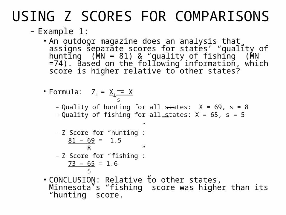
USING Z SCORES FOR COMPARISONS– Example 1:

• An outdoor magazine does an analysis that assigns separate scores for states’ “quality of hunting” (MN = 81) & “quality of fishing” (MN =74). Based on the following information, which score is higher relative to other states?

• Formula: Zi = Xi – X s

– Quality of hunting for all states: X = 69, s = 8– Quality of fishing for all states: X = 65, s = 5

– Z Score for “hunting”:81 – 69 = 1.5 8

– Z Score for “fishing”:73 – 65 = 1.6 5

• CONCLUSION: Relative to other states, Minnesota’s “fishing” score was higher than its “hunting” score.

USING Z SCORES FOR COMPARISONS– Example 2:

• You score 80 on a Sociology exam & 68 on a Philosophy exam. On which test did you do better relative to other students in each class?

Formula: Zi = Xi – X

s

– Sociology: X = 83, s = 10

– Philosophy: X = 62, s = 6

– Z Score for Sociology:

80 – 83 = - 0.3

10

– Z Score for Philosophy:

68 – 62 = 1

6

• CONCLUSION: Relative to others in your classes, you did better on the philosophy test

Normal curve table

For any standardized normal distribution, Appendix A (p. 453-456) of Healey provides precise info on:

the area between the mean and the Z score (column b)

the area beyond Z (column c) Table reports absolute values of Z scores

Can be used to find: The total area above or below a Z score The total area between 2 Z scores

THE NORMAL DISTRIBUTION Area above or below a Z score

If we know how many S.D.s away from the mean a score is, assuming a normal distribution, we know what % of scores falls above or below that score

This info can be used to calculate percentiles

AREA BELOW Z• EXAMPLE 1: You get a 58 on a Sociology test.

You learn that the mean score was 50 and the S.D. was 10.

– What % of scores was below yours?

Zi = Xi – X = 58 – 50 = 0.8

s 10

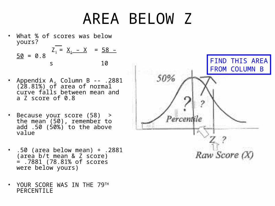
AREA BELOW Z• What % of scores was below

yours? Zi = Xi – X = 58 – 50 = 0.8

s 10

• Appendix A, Column B -- .2881 (28.81%) of area of normal curve falls between mean and a Z score of 0.8

• Because your score (58) > the mean (50), remember to add .50 (50%) to the above value

• .50 (area below mean) + .2881 (area b/t mean & Z score) = .7881 (78.81% of scores were below yours)

• YOUR SCORE WAS IN THE 79TH PERCENTILE

FIND THIS AREAFROM COLUMN B

AREA BELOW Z

– Example 2:– Your friend gets a 44 (mean = 50 & s=10) on the same

test– What % of scores was below his?

Zi = Xi – X = 44 – 50 = - 0.6

s 10

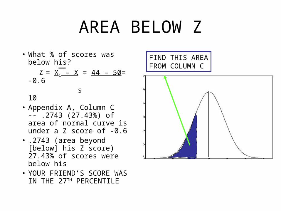
AREA BELOW Z

• What % of scores was below his?

Z = Xi – X = 44 – 50= -0.6 s 10• Appendix A, Column C

-- .2743 (27.43%) of area of normal curve is under a Z score of -0.6

• .2743 (area beyond [below] his Z score) 27.43% of scores were below his

• YOUR FRIEND’S SCORE WAS IN THE 27TH PERCENTILE

FIND THIS AREAFROM COLUMN C

Z SCORES: “ABOVE” EXAMPLE– Sometimes, lower is better…

• Example: If you shot a 68 in golf (mean=73.5, s = 4), how many scores are above yours?

68 – 73.5 = - 1.37 4

– Appendix A, Column B -- .4147 (41.47%) of area of normal curve falls between mean and a Z score of 1.37

– Because your score (68) < the mean (73.5), remember to add .50 (50%) to the above value

– .50 (area above mean) + .4147 (area b/t mean & Z score) = .9147 (91.47% of scores were above yours) FIND THIS

AREA FROM COLUMN B

68 73.5

Area between 2 Z Scores

What percentage of people have I.Q. scores between Stan’s score of 110 and Shelly’s score of 125? (mean = 100, s = 15)

CALCULATE Z SCORES

AREA BETWEEN 2 Z SCORES What percentage of people

have I.Q. scores between Stan’s score of 110 and Shelly’s score of 125? (mean = 100, s = 15) CALCULATE Z SCORES:

Stan’s z = .67 Shelly’s z = 1.67

Proportion between mean (0) & .67 = .2486 = 24.86%

Proportion between mean & 1.67 = .4525 = 45.25%

Proportion of scores between 110 and 125 is equal to: 45.25% – 24.86% = 20.39%

0 .67 1.67

AREA BETWEEN 2 Z SCORES EXAMPLE 2:

If the mean prison admission rate for U.S. counties was 385 per 100k, with a standard deviation of 151 (approx. normal distribution)

Given this information, what percentage of counties fall between counties A (220 per 100k) & B (450 per 100k)?

Answers: A: 220-385 = -165 = -1.09

151 151

B: 450-385 = 65 = 0.43

151 151

County A: Z of -1.09 = .3621 = 36.21%

County B: Z of 0.43 = .1664 = 16.64%

Answer: 36.21 + 16.64 = 52.85%

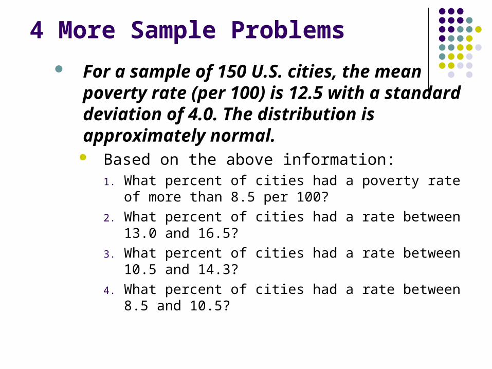
4 More Sample Problems

For a sample of 150 U.S. cities, the mean poverty rate (per 100) is 12.5 with a standard deviation of 4.0. The distribution is approximately normal.

Based on the above information:1. What percent of cities had a poverty rate of more than

8.5 per 100?

2. What percent of cities had a rate between 13.0 and 16.5?

3. What percent of cities had a rate between 10.5 and 14.3?

4. What percent of cities had a rate between 8.5 and 10.5?