NTIA Report 03-402

Measurements to Determine PotentialInterference to Public Safety Radio

Receivers from UltrawidebandTransmission Systems

J. Randy HoffmanEldon J. Haakinson

Yeh Lo

U.S. DEPARTMENT OF COMMERCEDonald L. Evans, Secretary

Fredrick R. Wentland, Acting Deputy Assistant Secretary for Communications and Information

June 2003

iii

DISCLAIMER

Certain commercial equipment, instruments, or materials are identified in this report tospecify the technical aspects of the reported results. In no case does such identificationimply recommendation or endorsement by the National Telecommunications and InformationAdministration, nor does it imply that the material or equipment identified is necessarily thebest available for the purpose.

v

CONTENTSPage

FIGURES . . . . . . . . . . . . . . . . . . . . . . . . . . . . . . . . . . . . . . . . . . . . . . . . . . . . . . . . . . . . . . . . . . . vi

TABLES . . . . . . . . . . . . . . . . . . . . . . . . . . . . . . . . . . . . . . . . . . . . . . . . . . . . . . . . . . . . . . . . . . . vii

EXECUTIVE SUMMARY . . . . . . . . . . . . . . . . . . . . . . . . . . . . . . . . . . . . . . . . . . . . . . . . . . . . . ix

ABSTRACT . . . . . . . . . . . . . . . . . . . . . . . . . . . . . . . . . . . . . . . . . . . . . . . . . . . . . . . . . . . . . . . . . . 1

1. INTRODUCTION . . . . . . . . . . . . . . . . . . . . . . . . . . . . . . . . . . . . . . . . . . . . . . . . . . . . . . . . . . . 11.1 The Technologies . . . . . . . . . . . . . . . . . . . . . . . . . . . . . . . . . . . . . . . . . . . . . . . . . . . . . 2

1.1.1 Ultrawideband Transmission Systems . . . . . . . . . . . . . . . . . . . . . . . . . . . . . 21.1.2 Public Safety Radio Systems . . . . . . . . . . . . . . . . . . . . . . . . . . . . . . . . . . . . 3

1.2 Scope . . . . . . . . . . . . . . . . . . . . . . . . . . . . . . . . . . . . . . . . . . . . . . . . . . . . . . . . . . . . . . 31.3 Organization of this Report . . . . . . . . . . . . . . . . . . . . . . . . . . . . . . . . . . . . . . . . . . . . . 3

2. SIGNAL CHARACTERISTICS . . . . . . . . . . . . . . . . . . . . . . . . . . . . . . . . . . . . . . . . . . . . . . . . 52.1 Public Safety LMR Systems . . . . . . . . . . . . . . . . . . . . . . . . . . . . . . . . . . . . . . . . . . . . 52.2 UWB Signals . . . . . . . . . . . . . . . . . . . . . . . . . . . . . . . . . . . . . . . . . . . . . . . . . . . . . . . . 5

3. MEASUREMENT SYSTEM AND PROCEDURES . . . . . . . . . . . . . . . . . . . . . . . . . . . . . . . . 93.1 System . . . . . . . . . . . . . . . . . . . . . . . . . . . . . . . . . . . . . . . . . . . . . . . . . . . . . . . . . . . . . 9

3.1.1 LMR Source Segment . . . . . . . . . . . . . . . . . . . . . . . . . . . . . . . . . . . . . . . . . 113.1.2 UWB Source Segment . . . . . . . . . . . . . . . . . . . . . . . . . . . . . . . . . . . . . . . . 113.1.3 CW Source Segment . . . . . . . . . . . . . . . . . . . . . . . . . . . . . . . . . . . . . . . . . . 133.1.4 Noise Source Segment . . . . . . . . . . . . . . . . . . . . . . . . . . . . . . . . . . . . . . . . 133.1.5 LMR Receiver Segment . . . . . . . . . . . . . . . . . . . . . . . . . . . . . . . . . . . . . . . 13

3.2 Measurement Procedure . . . . . . . . . . . . . . . . . . . . . . . . . . . . . . . . . . . . . . . . . . . . . . . 153.2.1 Digital-modulation (P25) Radio Receiver Measurement Procedure . . . . . 153.2.2 Analog FM Radio Receiver Measurement Procedure . . . . . . . . . . . . . . . . 16

3.3 Power Measures, Settings, Calibration and Frequency Precision . . . . . . . . . . . . . . . 183.3.1 Calibration and Power Level Correction . . . . . . . . . . . . . . . . . . . . . . . . . . 183.3.2 Frequency Precision . . . . . . . . . . . . . . . . . . . . . . . . . . . . . . . . . . . . . . . . . . 19

4. MEASUREMENT RESULTS . . . . . . . . . . . . . . . . . . . . . . . . . . . . . . . . . . . . . . . . . . . . . . . . 204.1 Description of Compiled Measurement Results . . . . . . . . . . . . . . . . . . . . . . . . . . . . 204.2 Summary of Measurement Results . . . . . . . . . . . . . . . . . . . . . . . . . . . . . . . . . . . . . . 34

5. CONCLUSION . . . . . . . . . . . . . . . . . . . . . . . . . . . . . . . . . . . . . . . . . . . . . . . . . . . . . . . . . . . . 35

6. ACKNOWLEDGMENTS . . . . . . . . . . . . . . . . . . . . . . . . . . . . . . . . . . . . . . . . . . . . . . . . . . . 37

vi

7. REFERENCES . . . . . . . . . . . . . . . . . . . . . . . . . . . . . . . . . . . . . . . . . . . . . . . . . . . . . . . . . . . . 37

8. ACRONYMS . . . . . . . . . . . . . . . . . . . . . . . . . . . . . . . . . . . . . . . . . . . . . . . . . . . . . . . . . . . . . . 38

APPENDIX: CHARACTERISTICS OF GENERATED UWB SIGNALS . . . . . . . . . . . . . . A-1A.1 Signal Description . . . . . . . . . . . . . . . . . . . . . . . . . . . . . . . . . . . . . . . . . . . . . . . . . A-1A.2 Residual Spectral Effects due to Signal Generation . . . . . . . . . . . . . . . . . . . . . . . A-2

FIGURESPage

Figure 2.1. Pulse spacing modes. . . . . . . . . . . . . . . . . . . . . . . . . . . . . . . . . . . . . . . . . . . . . . . . 6Figure 2.2. Spectral characteristics of the different pulse spacing modes. . . . . . . . . . . . . . . . . 7Figure 2.3. Temporal plots of 50%-ARD UWB signals passed through a 20-MHz bandpass

filter and downconverted to an intermediate frequency. . . . . . . . . . . . . . . . . . . . . 8Figure 3.1. Public Safety radio interference test bed. . . . . . . . . . . . . . . . . . . . . . . . . . . . . . . . . 9Figure 3.2. Block diagram of measurement system. . . . . . . . . . . . . . . . . . . . . . . . . . . . . . . . 10Figure 3.3. Frequency histogram of the C4FM modulated signal. . . . . . . . . . . . . . . . . . . . . . 11Figure 3.4. Input impedance to receiver A as seen at the input to the matching stub. . . . . . . 14Figure 3.5. Input impedance to receiver B as seen at the input to the matching stub. . . . . . . 14Figure 3.6. Basic block diagram for digital modulation radio receiver measurement. . . . . . 15Figure 3.7. Basic block diagram for analog radio receiver measurement. . . . . . . . . . . . . . . . 17Figure 4.1. In-band interference rejection (PREF ! PI). . . . . . . . . . . . . . . . . . . . . . . . . . . . . . 21Figure 4.2. Percent bit-error versus variable interference power density for Receiver A in P25

mode – 100-kHz PRF UWB interference. . . . . . . . . . . . . . . . . . . . . . . . . . . . . . . 25Figure 4.3. Percent bit-error versus variable interference power density for Receiver A in P25

mode – 20-MHz PRF UWB interference. . . . . . . . . . . . . . . . . . . . . . . . . . . . . . . 25Figure 4.4. Percent bit-error versus variable LMR power for Receiver A in P25 mode – 100-

kHz PRF UWB interference. . . . . . . . . . . . . . . . . . . . . . . . . . . . . . . . . . . . . . . . . 26Figure 4.5. Percent bit-error versus variable LMR power for Receiver A in P25 mode – 20-

MHz PRF UWB interference. . . . . . . . . . . . . . . . . . . . . . . . . . . . . . . . . . . . . . . . 26Figure 4.6. Percent bit-error versus variable interference power density for Receiver B in P25

mode – 100-kHz PRF UWB interference. . . . . . . . . . . . . . . . . . . . . . . . . . . . . . . 27Figure 4.7. Percent bit-error versus variable interference power density for Receiver A in P25

mode – 20-MHz PRF UWB interference. . . . . . . . . . . . . . . . . . . . . . . . . . . . . . . 27Figure 4.8. Percent bit-error versus variable LMR power for Receiver B in P25 mode – 100-

kHz PRF UWB interference. . . . . . . . . . . . . . . . . . . . . . . . . . . . . . . . . . . . . . . . . 28Figure 4.9. Percent bit-error versus variable LMR power for Receiver B in P25 mode – 20-

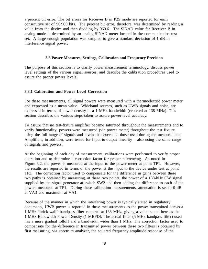
MHz PRF UWB interference. . . . . . . . . . . . . . . . . . . . . . . . . . . . . . . . . . . . . . . . 28Figure 4.10. Average SINAD versus variable interference power density for Receiver B in

analog mode – 100-kHz PRF UWB interference. . . . . . . . . . . . . . . . . . . . . . . . . 29Figure 4.11. Average SINAD versus variable interference power density for Receiver B in

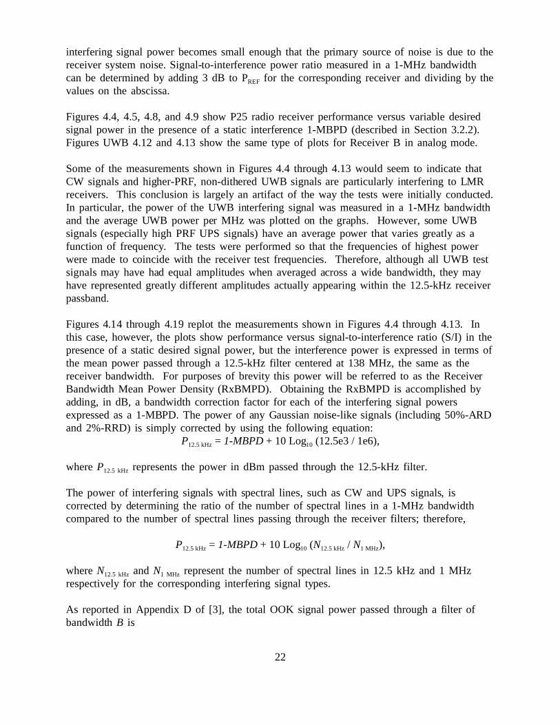
analog mode – 20-MHz PRF UWB interference. . . . . . . . . . . . . . . . . . . . . . . . . 29

vii

Figure 4.12. Average SINAD versus variable LMR power for Receiver B in analog mode –100-kHz PRF UWB interference. . . . . . . . . . . . . . . . . . . . . . . . . . . . . . . . . . . . . 30

Figure 4.13. Average SINAD versus variable LMR power for Receiver B in analog mode – 20-MHz PRF UWB interference. . . . . . . . . . . . . . . . . . . . . . . . . . . . . . . . . . . . . . . . 30

Figure 4.14. Percent bit-error versus S/I for Receiver A in P25 mode – 100-kHz PRF UWBinterference. . . . . . . . . . . . . . . . . . . . . . . . . . . . . . . . . . . . . . . . . . . . . . . . . . . . . . 31

Figure 4.15. Percent bit-error versus S/I for Receiver A in P25 mode – 20-MHz PRF UWBinterference. . . . . . . . . . . . . . . . . . . . . . . . . . . . . . . . . . . . . . . . . . . . . . . . . . . . . . 31

Figure 4.16. Percent bit-error versus S/I for Receiver B in P25 mode – 100-kHz PRF UWBinterference. . . . . . . . . . . . . . . . . . . . . . . . . . . . . . . . . . . . . . . . . . . . . . . . . . . . . . 32

Figure 4.17. Percent bit-error versus S/I for Receiver B in P25 mode – 20-MHz PRF UWBinterference. . . . . . . . . . . . . . . . . . . . . . . . . . . . . . . . . . . . . . . . . . . . . . . . . . . . . . 32

Figure 4.18. Average SINAD versus S/I for Receiver B in analog mode – 100-kHz PRF UWBinterference. . . . . . . . . . . . . . . . . . . . . . . . . . . . . . . . . . . . . . . . . . . . . . . . . . . . . . 33

Figure 4.19. Average SINAD versus S/I for Receiver B in analog mode – 20-MHz PRF UWBinterference. . . . . . . . . . . . . . . . . . . . . . . . . . . . . . . . . . . . . . . . . . . . . . . . . . . . . . 33

Figure A-1. Discrete binning of pulse position for clock referenced dithering. . . . . . . . . . A-3Figure A.3. Spectral lines due to discrete binning of pulse position. . . . . . . . . . . . . . . . . . . A-3

TABLES

Table 3.1. UWB Signal Space . . . . . . . . . . . . . . . . . . . . . . . . . . . . . . . . . . . . . . . . . . . . . . . . . 12Table 4.1. In-band Interference Rejection (PREF - PI) in dB . . . . . . . . . . . . . . . . . . . . . . . . . . . 20Table 4.2. Power Correction Factors (dB) . . . . . . . . . . . . . . . . . . . . . . . . . . . . . . . . . . . . . . . . 24Table A-1. Characteristics of Generated UWB Signals . . . . . . . . . . . . . . . . . . . . . . . . . . . . A-1

ix

EXECUTIVE SUMMARY

This report describes laboratory measurements to determine the extent and nature ofinterference to Public Safety radio receivers by ultrawideband (UWB) signals. Two PublicSafety radio receivers from different manufacturers were tested in the 138-MHz band, bothconfigured for Project 25 digital radio mode and one additionally configured and tested inanalog mode. The laboratory measurements were performed by inserting increasing levels ofUWB interference and measuring either bit-error rate (BER) for digital radios orsignal-plus-noise-plus-distortion to noise-plus-distortion ratio (SINAD) for one of the sameradios placed in analog mode.

When put through the passband of the receiver and analyzed in terms of the spectral andamplitude probability statistics, we see that all UWB signals, while initially impulsive, arealtered by the passband transfer function to take on characteristics that lie along a continuumfrom impulsive, to Gaussian noise-like, to sinusoidal. By varying pulse repetition frequency(PRF), pulse spacing schemes, and gating, a variety of UWB signals were generated forthese measurements. However, because of the relatively narrow bandwidths of the receiverpassband (12.5 kHz), none of the interfering signals were considered impulsive afteralteration by the receiver passband transfer function. To be impulsive would have requiredPRFs significantly less than 12.5 kHz.

Results showed that, when reported in terms of average UWB power in the receiverbandwidth, there is little difference in interference to Public Safety radios when comparingeach of the generated UWB signal types. When expressed in terms of signal-to-interferencepower ratio, where interference power is defined as the power passed through the receiverpassband, reference sensitivity (5% BER for digital radios and 12 dB SINAD for analogradios) occurs at approximately 10 dB, with a variation of 2 to 5 dB on either side,depending upon the receiver and signal type. However, there are subtle trends, with gatedsignals being slightly more invasive and signals with spectral lines being slightly lessinvasive than signals that are Gauusian noise-like when altered by the receiver passbandtransfer function. When the interference power is expressed in terms of anything other thanthe mean power in the receiver bandwidth (e.g., wider bandwidths or peak power), thereceiver response can vary greatly depending upon the nature of the interfering signal.

† The authors are with the Institute for Telecommunication Sciences, National Telecommunications and

Information Administration, U.S. Department of Commerce, Boulder, CO 80305.

MEASUREMENTS TO DETERMINE POTENTIAL INTERFERENCE TO PUBLICSAFETY RADIO RECEIVERS FROM ULTRAWIDEBAND TRANSMISSION

SYSTEMS

J. Randy Hoffman, Eldon J. Haakinson, Yeh Lo†

This report describes laboratory measurements to determine the extent and natureof interference to Public Safety radio receivers by ultrawideband (UWB) signals. Two Public Safety radio receivers from different manufacturers were tested in the138-MHz band, both configured for Project 25 digital radio mode and oneadditionally configured and tested in analog mode. The laboratorymeasurements were performed by inserting increasing levels of UWB interferenceand measuring either bit-error rate (BER) for digital radios orsignal-plus-noise-plus-distortion to noise-plus-distortion ratio (SINAD) for one ofthe same radios placed in analog mode. By varying pulse repetition frequency(PRF), pulse spacing schemes, and gating, a variety of UWB signals weresimulated, which were either Gaussian noise-like, sinusoidal, or a hybrid of thetwo when passed through the receiver passband. Results showed that, whenreported in terms of average UWB power in the receiver bandwidth, there is littledifference in interference to Public Safety radios when comparing each of thegenerated UWB signal types. When expressed in terms of signal-to-interferencepower ratio, where interference power is defined as the power passed through thereceiver passband, reference sensitivity (5% BER for digital radios and 12 dBSINAD for analog radios) occurs at approximately 10 dB, with a variation of 2to 5 dB on either side, depending upon the receiver and signal type. When theinterference power is expressed in terms of anything other than the mean powerin the receiver bandwidth (e.g., wider bandwidths or peak power), the receiverresponse can vary greatly depending upon the nature of the interfering signal.

Key words: impulse radio, interference measurement, noise, Project 25, Public Safety radiosystems, radio frequency interference (RFI), ultrawideband (UWB)

1. INTRODUCTION

As new wireless applications and technologies continue to develop, conflicts in spectrum useand system incompatibility are inevitable. This report investigates potential interference toPublic Safety radio receivers by ultrawideband (UWB) signals. According to Part 15 of theFederal Communications Commission (FCC) rules, non-licensed operation of low-powertransmitters is allowed if interference to licensed radio systems is negligible. On May 11,2000, the FCC issued a Notice of Proposed Rulemaking (NPRM) [1] which proposed that

2

UWB devices operate under Part 15 rules. This would exempt UWB systems from licensingand frequency coordination and allow them to operate under a new UWB section of Part 15,based on claims that UWB devices can operate on spectrum already occupied by existingradio services without causing interference. The NPRM called for further testing andanalysis to investigate the risks of UWB interference and ensure that critical radio servicesare adequately protected.

Conventional methods for measuring and quantifying interference under narrowbandassumptions are insufficient for testing UWB interference. Recently, the NationalTelecommunications and Information Administration’s (NTIA’s) Institute forTelecommunication Sciences (ITS) studied the general characteristics of UWB signals [2]and the effects of UWB signals on global positioning systems [3] [4]. As a naturalextension to these studies, this report describes the investigation of interference from arepresentative set of UWB signals imposed on a select group of Public Safety radioreceivers. The remainder of this section discusses the relevant technologies and associatedapplications, briefly summarizes related studies, and gives an outline for this report.

1.1 The Technologies

The multifaceted strategic and commercial importance, as well as potential for conflict, ofPublic Safety radio and UWB systems are summarized in the following subsections.

1.1.1 Ultrawideband Transmission Systems

Unlike conventional radio systems, UWB devices bypass intermediate frequency stages,possibly reducing complexity and cost. Additionally, the high cost of frequency allocationfor these devices is avoided if they are allowed to operate under Part 15 rules. Thesepotential advantages have been a catalyst for the development of UWB technologies.

UWB signals are characterized by modulation methods that vary pulse timing and positionrather than carrier-frequency, amplitude, or phase. Short pulses (on the order of ananosecond) spread their power across a wide bandwidth rather than containing it in anarrow band. UWB proponents argue that the power spectral density decreases below thethreshold of narrowband receivers, minimizing interference. Other possible advantages aremitigation of frequency selective fading induced by multipath or transmission throughmaterials.

Existing and potential applications for UWB technology can be divided into two groups –wireless communications and short-range sensing. In wireless communications, UWB hasbeen claimed to be an effective way to link many users in multipath environments (e.g.,distribution of wireless services throughout a home or office). In short-range sensing

3

applications, it can be used for determining structural soundness of bridges, roads, andrunways and locating objects and utilities underground. Potential automotive uses includecollision avoidance systems, air bag proximity measurement for safe deployment, and fluidlevel detectors. UWB technology is being developed for new types of imaging systems thatwould assist rescue personnel in locating persons hidden behind walls, under debris, or undersnow.

1.1.2 Public Safety Radio Systems

Public Safety agencies, including law enforcement, fire, and emergency medical services, useland mobile radio (LMR) systems for communication of voice and data messages. It isanticipated that UWB applications such as ground-penetration radars and through-the-wall-imaging systems will operate with the spectral region of greatest power located below1 GHz. The Public Safety user might rely on these UWB systems to operate in closeproximity to LMR systems under the same operational scenarios – to provide both vitalcommunications and search/rescue sensor information. For these reasons, it is important todetermine the potential of interference to LMR Public Safety radio systems from UWBemissions.

1.2 Scope

The objective of these measurements is to measure the interference by different classes ofUWB signals to several different Public Safety radio receivers and to observe and reportbroad trends in Public Safety LMR performance to this interference. No attempt is made toevaluate specific receiver designs or interference mitigation strategies or provide precisedegradation criteria. Recommendations on UWB regulation, likewise, are not addressed andlie under the jurisdiction of the policy teams at NTIA’s Office of Spectrum Management andthe FCC.

1.3 Organization of this Report

Investigation of UWB interference to Public Safety LMR systems encompasses a broad rangeof expertise including LMR theory of operation, RF design and hardware implementation,and temporal and spectral characterization of interfering signals. This report completelydescribes the experiment and is organized as follows.

The first three sections provide orientation and background for the reader. Section 2describes Public Safety LMR and UWB signal characteristics in order to identify potentialinterference scenarios and rationalize measurement procedures. Section 3 gives a detailedsummary of the measurement system, test procedures, UWB-signal sample space, signalgeneration details, and hardware limitations. Section 4 provides and summarizes the

4

measurement results. Conclusions are drawn in Section 5. The appendix provides a detaileddescription of each UWB type under test.

†Project 25 (P25) is a standard developed for Public Safety LMR radio systems to providedigital, narrowband radios with the best performance possible and to permit maximuminteroperability. These standards are a joint effort of U.S. Federal, state, and local governments,with support from the U.S. Telecommunications Industry Association (TIA). State Governmentis represented by the National Association of State Telecommunications Directors (NASTD) andlocal government by the Association of Public-safety Communications Officials, International(APCO).

5

2. SIGNAL CHARACTERISTICS

The purpose of this section is to describe Public Safety LMR and UWB signal characteristicsin order to identify potential interference scenarios and rationalize measurement procedures.

2.1 Public Safety LMR Systems

Public Safety LMR systems operate in various bands from about 30 MHz to 900 MHz, withbandwidths currently 25-30 kHz; new regulations, however, require the bandwidths to bereduced to 12.5 kHz (and potentially to 6.25 kHz). Both digital and analog modulationschemes are currently utilized for Public Safety LMR communications. For thesemeasurements, two types of modulation standards were used – Project 25† digital signals andtraditional analog signals. The Project 25 radios used in these measurements have a 4-levelfrequency shift keyed (C4FM) modulation confined to 12.5-kHz bands. Two-bit symbols arerepresented by 4 different frequency shifts, each separated by 1.2 kHz. The analog radio-configuration used for these measurements has a 12.5-kHz bandwidth and employs afrequency modulation (FM).

2.2 UWB Signals

The UWB signal is, in general, a sequence of narrow pulses with widths on the order of 0.2to 10 ns. Uniform pulse spacing (UPS), as the name implies, means the UWB signal has nomodulation and the pulses are spaced equally apart. Modulation of the pulses can take onmany different forms. One form of digital modulation is pulse-position modulation where,for example, a pulse that is slightly advanced from its nominal position represents a “zero.”Likewise, a slightly retarded pulse represents a “one.” Another form of digital modulation ison-off keying (OOK) where pulses, in what is normally an evenly spaced sequence, aredeleted, thus representing “zeros.” In addition to the modulation scheme, the pulses can bedithered, where pulses are randomly located relative to their nominal, periodic location –absolute referenced dithering (ARD), or relative to the previous pulse – relative referenceddithering (RRD). The extent of dither is expressed in terms of the percentage of pulserepetition period, which is the reciprocal of pulse repetition frequency (PRF). For example,50% absolute referenced dithering describes a situation where the pulse is randomly located

†While Figure 2.2 shows spectral plots at a center frequency of 1575 MHz, the principlespresented herein apply, as well, to the 138-MHz band of interest.

6

Figure 2.1. Pulse spacing modes.

in the first half of the period following the nominal pulse location. Finally, some UWBsystems employ gating. This is a process whereby the pulse train is turned on for sometime and off for the remainder of a gating period.

Four different pulse spacing modes (UPS, OOK, ARD, and RRD) are illustrated inFigure 2.1, whereby the vertical dashed lines represent the ticks of a clock. Gating isrepresented by the removal of the pulses in the shaded areas; in the case of the UPSexample, there are 4 pulses generated during the gated-on time followed by 8 clock ticks forwhich there are no pulses (to give a duty cycle of 33%).

Spectral Considerations

The frequency domain characteristics (emission spectrum) of a UWB signal are dependentupon the time-domain characteristics described above. The pulse shape/width determines theoverall spectral envelope, where the bandwidth is approximately equal to the reciprocal ofthe pulse width. The manner in which the pulses are sequentially spaced determines the finespectral features within the confines of the envelope.

Spectral plots are shown in Figure 2.2 for four different UWB signals as they are passedthrough a bandpass filter.† UPS has the power gathered up into spectral lines at intervals ofthe PRF. The greater the PRF, the wider the line spacing, and the greater the powercontained in each spectral line. OOK also has spectral lines spaced at intervals of the PRFthat are superimposed on a continuous noise-like spectrum. Dithered signals have spectralcharacteristics inherently different from either UPS or OOK. For these measurements, ARDhas a pulse spacing that is varied by 50% of the referenced clock period. RRD has a pulse

7

Figure 2.2. Spectral characteristics of the different pulse spacingmodes.

spacing that is varied by 2% of the average pulse period. Both of these dithered cases havespectral features that are characteristic of noise (i.e., no spectral lines). The reader isreferred to references [2] and [3] for a more in-depth discussion of the spectralcharacteristics of UWB signals.

Another feature worth noting is the phenomenon of spectral lines spreading due to gating. The spectrum of the gated UWB signal is the result of convolving the non-gated signal withthat of a rectangular function, the latter of whose Fourier transform amplitude has asinc-squared envelope characteristic. It follows that the single line of the non-gated cases isspread out into a multitude of lines confined by the sinc-squared envelope, where thespacing between lines, or line spread spacing (LSS), is equal to the reciprocal of the gatingperiod; null spacing, or line spreading null-to-null bandwidth (LSNB), of the main lobe ofthe sinc-squared function is equal to two times the reciprocal of gated-on time.

There are two additional spectral features that occur as a result of the signals having beengenerated by an arbitrary waveform generator (AWG). One is related to how the pattern ofpulses is repeated, and the other has to do with the process of placing the pulses into bins,representing discrete dithered pulse spacing. Further discussion of these spectralcharacteristics of UWB signals is contained in the appendix.

8

Figure 2.3. Temporal plots of 50%-ARD UWB signals passedthrough a 20-MHz bandpass filter and downconvertedto an intermediate frequency.

Temporal Characteristics

When a narrow pulse, with a wide bandwidth (BW), is passed through a filter with anarrower bandwidth, the output is essentially equal to the impulse response of the filter; theresultant output has a pulse width approximately equal to the reciprocal of the receiverbandwidth and oscillates at the center frequency of the filter. Figure 2.3 illustrates50%-ARD signals, at three different PRFs, passed through a 20-MHz bandpass filter(downconverted to an intermediate frequency); the appearance is that of a sinusoid turned onfor intervals of 50 ns. The result is that, as the pulse passes through the filter, it becomeswider, the peak-to-average power ratio decreases, and depending upon the PRF and extent ofdithering, the pulses may overlap. Because the phase of the oscillation is dependent uponthe time origin of the pulse, the phase for adjacent dithered pulses can be asynchronous.This can result in constructive and destructive summation of signal components foroverlapping pulses, giving the appearance of random, noise-like signals. OOK signals, whilesynchronous in phase for adjacent pulses, can have a similar noise-like appearance whenadjacent pulses overlap.

9

Figure 3.1. Public Safety radio interference test bed.

3. MEASUREMENT SYSTEM AND PROCEDURES

The purpose of this section is to provide a detailed summary of the measurement system, test procedures, UWB-signal sample space, signal generation details, and hardwarelimitations for this experiment.

3.1 System

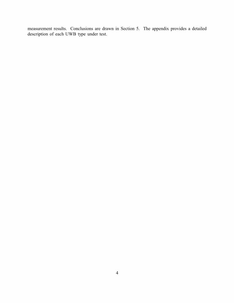
The experimental setup (see Figure 3.1) was comprised of five segments – LMR source,UWB source, continuous-wave (CW) source, noise source, and radio receiver. The systemconfiguration is illustrated in Figure 3.2. Each of the wideband sources (i.e., noise andUWB) were filtered, amplified, and combined prior to input into the receiver. Signal powerswere controlled using precision variable attenuators (VA1, VA2, and VA3). The followingsubsections provide signal-generation details and justification for hardware employed.

Figure 3.2. Block diagram of measurement system.

†The UWB pulse generator used in these measurements is a Time Domain PG-2000 withimpulse voltage rise time (10 - 90%) = 200 ps, impulse fall time (90 - 10%) = 416 ps, impulsewidth (50%) = 521 ps, and no nulls in the 138-MHz band.

11

Figure 3.3. Frequency histogram of the C4FMmodulated signal.

3.1.1 LMR Source Segment

The purpose of the LMR signal segment is to provide an emulated Public Safety LMR radiosignal. The LMR signal was generated with a Motorola R-2670 Communications Test Set,the output being a digital test tone using a 1.011-kHz CW bit pattern with C4FMmodulation. Figure 3.3 shows a frequency histogram of the generated signal as measured ona modulation domain analyzer (all equipment referenced with a rubidium oscillator). Theanalog test signal was generated by using a 1.0-kHz modulating signal and setting themaximum frequency deviation to 3 kHz. The center frequency for both signal types was138 MHz. The R-2670 Communication System Analyzer served the additional role of aSINAD meter for analog testing.

3.1.2 UWB Source Segment

The UWB segment consists of a narrow-pulse generator and a triggering device (either anarbitrary waveform generator or a custom built relative-referenced triggering device) to createvarious signals. Because the pulse shape/width of the UWB signal determines the spectralenvelope of the signal, the primary criterion for choosing a UWB pulse generator for thesemeasurements was whether the spectral envelope has no nulls and produces sufficient poweracross the 138-MHz band of interest.†

12

UWB Signal Space

For these measurements, the UWB signal is specified by a combination of mode-of-spacing,PRF, and the application of gating. By varying these three parameters, 11 differentpermutations were chosen to span a reasonable range of existing and potential UWB signals. For these measurements (as shown in Table 3.1) there are two PRFs (0.1 and 20 MHz), fourpulse spacing modes (UPS, OOK, 50%-ARD, and 2%-RRD), and two gating scenarios (nogating and 20% gating with a 4 ms on-time). In addition to these 11 permutations, formeasurements with C4FM modulated transmissions, each of the UWB signals with spectrallines have two separate conditions of spectral alignment in relation to the spectral bins notedin Figure 3.3 – one with a spectral line at 138.000506 MHz (aligned with a C4FMfrequency shift) and the other with a spectral line at 137.999862 (offset from any C4FMfrequency shift). Three of the interference signal types were added as the measurementswere in progress, and therefore, were only included with the measurements on one of thereceivers; these additional UWB signal types consisted of: 1) 100-kHz PRF, UPS, gated,aligned, 2) 100-kHz PRF, UPS, gated, offset, and 3) 100-kHz PRF, ARD, gated.

Table 3.1. UWB Signal Space

PRF Pulse Spacing Mode Gating Spectral Alignment

100 kHz UPS None Aligned

100 kHz UPS None Offset

100 kHz UPS Gated Aligned

100 kHz UPS Gated Offset

100 kHz OOK None Aligned

100 kHz OOK None Offset

100 kHz ARD None N/A

100 kHz ARD Gated N/A

100 kHz RRD None N/A

20 MHz UPS None Aligned

20 MHz UPS None Offset

20 MHz UPS Gated Aligned

20 MHz UPS Gated Offset

20 MHz OOK None Aligned

Con’t Table 3.1. UWB Signal Space

PRF Pulse Spacing Mode Gating Spectral Alignment

13

20 MHz OOK None Offset

20 MHz RRD None N/A

20 MHz RRD Gated N/A

3.1.3 CW Source Segment

The CW source segment simply consists of a sinusoidal signal produced by a signalgenerator. The purpose of this segment is to emulate a single spectral line so as to comparethe resulting interference to UWB signals also with spectral lines.

3.1.4 Noise Source Segment

The noise source segment consists of Gaussian noise produced by a noise diode. Thepurpose of this segment is to emulate Gaussian noise interference so as to compare theresulting interference to UWB signals that also have Gaussian noise-like characteristics.

3.1.5 LMR Receiver Segment

Two receivers, A and B, from two different Project 25 (P25) radio manufacturers, were usedfor measurement. Both receivers were programmed and tested in the P25 digital mode witha 12.5-kHz bandwidth, transmitting in the 138-MHz band. In addition, receiver B was, at alater point, programmed and tested in an analog FM mode, also with a carrier frequency of138 MHz. Via network analyzer, each device was characterized for input impedance with theradios set to the 138-MHz band. So as to match (zero-reflection) the input impedance to thecharacteristic impedance of the 50 S cables, matching stubs were designed and placed at theantenna input of each radio receiver during measurements. Using a network analyzer to makemeasurements, Figures 3.4 and 3.5 show the resulting input impedance with the matchingstubs in place. From these diagrams, it is clearly seen that the receivers’ antenna inputs(after inserting the matching stubs) were closely matched to 50 S real impedance withessentially no imaginary component. So as to reduce any coupling of radiated emission intothe receivers, each receiver was placed in a shielded box during measurements.

14

Figure 3.4. Input impedance to receiver A as seen at the input tothe matching stub.

Figure 3.5. Input impedance to receiver B as seen at the input to thematching stub.

15

Figure 3.6. Basic block diagram for digital modulation radio receiver measurement.

3.2 Measurement Procedure

The measurements are performed using the test setup as shown in Figure 3.2. The unwantedsignal (UWB, CW, or Gaussian noise) is filtered, amplified, combined with the desired LMRsignal, and injected into the Public Safety radio receiver at the antenna port of the receiverunder test. Each of the individual signals (unwanted and desired) is independently measuredfor power using a power meter, with power translated (using calibration factors) to that atthe input of the LMR receiver antenna port. For the digital-modulation receivers,measurements are conducted using a 5% BER performance threshold with a UWB signal,CW signal, and Gaussian noise (each separately) as the interfering source. For the analogFM receiver, the same interfering sources are used, but susceptibility measurements areconducted using a 12-dB SINAD performance threshold.

3.2.1 Digital-modulation (P25) Radio Receiver Measurement Procedure

The digital modulation (P25) radio receivers are tested using the process defined in theProject 25 Standards document TIA/EIA-102.CAAA [5]. The procedure described, however,is modified by replacing the description of co-channel interference rejection with in-bandinterference rejection and making additional desired-signal to interference ratio measurements.

The in-band interference rejection is the ratio of the reference sensitivity to the level of anunwanted input signal. The unwanted signal has an amplitude that causes the BER producedby a wanted signal 3 dB in excess of the reference sensitivity (see definition in step 2below) to be reduced to the standard BER (in this case, 5%). The method of measurementis described as follows:

1. System configuration: The measurement setup is configured as illustrated in Figure 3.6,with the unwanted signal source connected to terminal B of the combining network.

16

2. Reference power of desired signal in absence of the interfering signal: In the absenceof the unwanted signal (VA2 set to maximum attenuation), the standard 1.011 kHzC4FM modulated tone is applied to terminal A of the combining network. The signallevel is reduced to obtain reference sensitivity, defined as the minimum acceptableperformance level (MAPL) without an interfering signal. [Note: For P25 receivers, theMAPL occurs with a BER of 5%.] This level is recorded in dBm as PREF.

3. Performance versus variable interference power density in the presence of a staticdesired signal power: a. The level of the wanted input signal is increased by 3 dB and the BER value

recorded. b. The unwanted input signal (UWB, noise, or CW signal) is applied to terminal B of

the combining network.c. The unwanted input signal power is increased to reestablish the MAPL. This level is

recorded in dBm as PI.d. The in-band interference rejection is calculated as follows:

in-band interference rejection = PREF - PI.e. The unwanted input signal power is reduced 10 dB in 1-2 dB steps. The level of the

unwanted input signal is recorded along with the corresponding value of BER at eachstep.

4. Performance versus variable desired signal power in the presence of a staticinterference power density:a. The unwanted input signal power is reduced to reestablish the MAPL (PI).b. The level of the wanted input signal is increased approximately 10 dB in 1-2 dB

steps. The level of the wanted input signal is recorded along with the correspondingvalue of BER at each step.

3.2.2 Analog FM Radio Receiver Measurement Procedure

The analog FM radio receivers are tested using a modified version of the process as definedin the FM/PM Standards document TIA/EIA-603. [6] The procedure described, however, ismodified by replacing the description of adjacent-channel interference rejection with in-bandinterference rejection and making additional desired-signal to interference ratio measurements.

Once again, the in-band interference rejection is the ratio of the reference sensitivity to thelevel of an unwanted input signal. The unwanted signal has an amplitude that causes theSINAD produced by a wanted signal 3 dB in excess of the reference sensitivity (seedefinition in step 2 below) to be reduced to the standard SINAD (in this case, 12 dB). Themethod of measurement is described as follows:

1. System configuration: The measurement setup is configured as illustrated in Figure 3.7,with the unwanted signal source connected to terminal B of the combining network.

17

Figure 3.7. Basic block diagram for analog radio receiver measurement.

2. Reference power of desired signal in absence of the interfering signal: In the absenceof the unwanted signal (VA2 set to maximum attenuation), the standard 1.0-kHz FMmodulated tone (3-kHz maximum frequency deviation) is applied to terminal A of thecombining network. The signal level is reduced to obtain MAPL without an interferingsignal. [Note: For Public Safety analog FM receivers, the MAPL occurs with a SINADof 12 dB.] This level is recorded in dBm as PREF.

3. Performance versus variable interference power density in the presence of a staticdesired signal power: a. The wanted input signal power is increased by 3 dB and the SINAD value recorded.b. The unwanted input signal (UWB, noise, or CW signal) is applied to terminal B of

the combining network.c. The unwanted input signal power is increased to reestablish the MAPL. This level is

recorded in dBm as PI.d. The in-band interference rejection is calculated as follows:

in-band interference rejection = PREF - PI.e. The unwanted input signal power is reduced 10 dB in 1-2 dB steps. The level of the

unwanted input signal is recorded along with the corresponding value of SINAD ateach step.

4. Performance versus variable desired signal power in the presence of a staticinterference power density:a. The unwanted input signal power is reduced to reestablish the MAPL (PI).b. The wanted input signal power is increased approximately 10 dB in 1-2 dB steps.

The level of the wanted input signal is recorded along with the corresponding valueof SINAD at each step.

Because of receiver differences with regard to the way BER and SINAD are determined,there are some variations in sample size between the different receivers and their modulationmodes. The bit errors for Receiver A are reported for each consecutive set of 1728 bits. Aminimum of 20 of these values were recorded, averaged, and then divided by 17.28 to give

18

a percent bit error. The bit errors for Receiver B in P25 mode are reported for eachconsecutive set of 96,960 bits. The percent bit error, therefore, was determined by reading avalue from the device and then dividing by 969.6. The SINAD value for Receiver B inanalog mode is determined by an analog SINAD meter located in the communication testset. A large enough population was sampled to give a standard deviation of 1 dB ininterference signal power.

3.3 Power Measures, Settings, Calibration and Frequency Precision

The purpose of this section is to clarify power measurement terminology, discuss powerlevel settings of the various signal sources, and describe the calibration procedures used toassure the proper power levels.

3.3.1 Calibration and Power Level Correction

For these measurements, all signal powers were measured with a thermoelectric power meterand expressed as a mean value. Wideband sources, such as UWB signals and noise, areexpressed in terms of power density in a 1-MHz bandwidth (centered at 138 MHz). Thissection describes the various steps taken to assure power-level accuracy.

To assure that no test-fixture amplifier became saturated throughout the measurements and toverify functionality, powers were measured (via power meter) throughout the test fixtureusing the full range of signals and levels that exceeded those used during the measurements.Amplifiers, in addition, were tested for input-to-output linearity – also using the same rangeof signals and powers.

At the beginning of each day of measurement, calibrations were performed to verify properoperation and to determine a correction factor for proper referencing. As noted inFigure 3.2, the power is measured at the input to the power meter at point TP1. However,the results are reported in terms of the power at the input to the device under test at pointTP3. The correction factor used to compensate for the difference in gains between thesetwo paths is obtained by measuring, at these two points, the power of a 138-kHz CW signalsupplied by the signal generator at switch SW2 and then adding the difference to each of thepowers measured at TP1. During these calibration measurements, attenuation is set to 0 dBat VA3 and maximum at VA1.

Because of the manner in which the interfering power is typically stated in regulatorydocuments, UWB power is reported in these measurements as the power transmitted across a1-MHz “brick-wall” bandpass filter centered at 138 MHz, giving a value stated here as the1-MHz Bandwidth Power Density (1-MBPD). The actual filter (5-MHz bandpass filter) usedhas a more gradual rolloff and a bandwidth wider than 1 MHz. The correction factor used tocompensate for the difference in transmitted power between these two filters is obtained byfirst measuring, via spectrum analyzer, the squared frequency amplitude response of the

19

“actually-used” filter for each wideband interfering signal (UWB signal and Gaussian noise).To obtain the transmitted power received through the filters, the resulting functions for eachof the wideband signals are integrated over the entire band between the stopbands of the“actually-used” filter and then once again across a 1-MHz bandwidth centered at 138 MHz. The correction factor for each wideband signal is the difference in dB of the transmittedpower through the “actually-used” filter and the “brick-wall” filter.

Another issue regarding power settings has to do with measuring and setting the power ofgated signals. Because the reaction time of a power meter is too fast to allow accuratemeasurement of gated signals, the power meter was configured to average 20 separatereadings; this procedure (empirically determined) stabilized the output of the meter andshowed values consistent with the non-gated case – a difference of 7 dB. (Twenty percentgating reduces mean non-gated signal power by 7 dB.) The power of all gated signals usedduring these interference measurements is expressed, depending upon the circumstance, aseither the average power or the average power of the equivalent non-gated signal (i.e., thepower of the gated-on time portion of the signal).

3.3.2 Frequency Precision

Because it is necessary to precisely place spectral lines of the interfering signals in relationto the spectral features of the desired signal (within a few tens of Hz), it is necessary toreference several instruments with a single oscillator. For these measurements, a rubidiumoscillator was used to reference the AWG, the desired signal source (MotorolaCommunications Test Set), the CW signal source, and the spectrum analyzer.

20

4. MEASUREMENT RESULTS

The purpose of this section is to describe the tabular and graphical compilation of themeasurements results and, in turn, to summarize. Conclusions are provided in the subsequentsection.

4.1 Description of Compiled Measurement Results

The powers of the desired signals at MAPL (PREF) for Receiver A (P25 mode), Receiver B(P25 mode), and Receiver B (analog mode) are !121 dBm, !117 dBm, and !119 dBmrespectively. Table 4.1 shows the in-band interference rejection for receiver A (P25 mode)and receiver B (P25 and analog modes) when subjected to the various UWB signals,Gaussian noise, and CW signals – all powers measured in a 1-MHz bandwidth. Figure 4.1shows the same data in a graphical form. Lower interference rejection values indicate thatthe interference source is less harmful. Thus, these data show that, when using the 1-MBPDmethod of measurement, Gaussian noise at a -12 dB rejection value is more benign than aCW signal which has a 6 or 7 dB rejection value. While the labels show signals withspectral lines to be “aligned” or “offset” (as described in Section 3.1.2), this only applies tothe receivers in P25 mode and does not apply to the analog case. As mentioned in Section3.1.2, three additional measurements were added to Receiver B as the measurements were inprogress, and therefore are not included in the results for Receiver A; this is denoted bydashed lines in Table 4.1.

Table 4.1. In-band Interference Rejection (PREF - PI) in dB

Signal TypeReceiver

Receiver A - P25 Mode

Receiver B - P25 Mode

Receiver B -Analog Mode

Gaussian Noise -12 -13 -15

CW, Aligned 7 6 3

CW, Offset 6 7 N/A

UWB, 100-kHz PRF, UPS, Non-gated, Aligned -3 -5 -6

UWB, 100-kHz PRF, UPS, Non-gated, Offset -4 -5 N/A

UWB, 100-kHz PRF, UPS, Gated, Aligned ----- -10 -10

UWB, 100-kHz PRF, UPS, Gated, Offset ----- -11 N/A

UWB, 100-kHz PRF, OOK, Non-gated, Aligned -5 -5 -7

UWB, 100-kHz PRF, OOK, Non-gated, Offset -6 -4 N/A

UWB, 100-kHz PRF, ARD, Non-gated -11 -12 -14

UWB, 100-kHz PRF, ARD, Gated ----- -21 -20

Con’t Table 4.1. In-band Interference Rejection (PREF - PI) in dB

Signal TypeReceiver

Receiver A - P25 Mode

Receiver B - P25 Mode

Receiver B -Analog Mode

21

Figure 4.1. In-band interference rejection (PREF ! PI).

UWB, 100-kHz PRF, RRD, Non-gated -10 -11 -14

UWB, 20-MHz PRF, UPS, Non-gated, Aligned 8 6 4

UWB, 20-MHz PRF, UPS, Non-gated, Offset 4 5 N/A

UWB, 20-MHz PRF, UPS, Gated, Aligned 0 -1 0

UWB, 20-MHz PRF, UPS, Gated, Offset -1 -1 N/A

UWB, 20-MHz PRF, OOK, Non-gated, Aligned 8 6 3

UWB, 20-MHz PRF, OOK, Non-gated, Offset 6 5 N/A

UWB, 20-MHz PRF, RRD, Non-gated -11 -13 -17

UWB, 20-MHz PRF, RRD, Gated -20 -20 -24

Figures 4.2, 4.3, 4.6, and 4.7 show P25 radio receiver performance versus variableinterference 1-MBPD in the presence of a static desired signal power (described in Section3.2.1). Figures 4.10 and 4.11 show the same type of plots for Receiver B in analog mode.The thick horizontal line in all of these graphs represents the receiver performance when theLMR signal is held 3 dB above reference sensitivity and no interfering signal is beinginjected; therefore each of the plots should asymptotically approach this line as the

22

interfering signal power becomes small enough that the primary source of noise is due to thereceiver system noise. Signal-to-interference power ratio measured in a 1-MHz bandwidthcan be determined by adding 3 dB to PREF for the corresponding receiver and dividing by thevalues on the abscissa.

Figures 4.4, 4.5, 4.8, and 4.9 show P25 radio receiver performance versus variable desiredsignal power in the presence of a static interference 1-MBPD (described in Section 3.2.2). Figures UWB 4.12 and 4.13 show the same type of plots for Receiver B in analog mode.

Some of the measurements shown in Figures 4.4 through 4.13 would seem to indicate thatCW signals and higher-PRF, non-dithered UWB signals are particularly interfering to LMRreceivers. This conclusion is largely an artifact of the way the tests were initially conducted. In particular, the power of the UWB interfering signal was measured in a 1-MHz bandwidthand the average UWB power per MHz was plotted on the graphs. However, some UWBsignals (especially high PRF UPS signals) have an average power that varies greatly as afunction of frequency. The tests were performed so that the frequencies of highest powerwere made to coincide with the receiver test frequencies. Therefore, although all UWB testsignals may have had equal amplitudes when averaged across a wide bandwidth, they mayhave represented greatly different amplitudes actually appearing within the 12.5-kHz receiverpassband.

Figures 4.14 through 4.19 replot the measurements shown in Figures 4.4 through 4.13. Inthis case, however, the plots show performance versus signal-to-interference ratio (S/I) in thepresence of a static desired signal power, but the interference power is expressed in terms ofthe mean power passed through a 12.5-kHz filter centered at 138 MHz, the same as thereceiver bandwidth. For purposes of brevity this power will be referred to as the ReceiverBandwidth Mean Power Density (RxBMPD). Obtaining the RxBMPD is accomplished byadding, in dB, a bandwidth correction factor for each of the interfering signal powersexpressed as a 1-MBPD. The power of any Gaussian noise-like signals (including 50%-ARDand 2%-RRD) is simply corrected by using the following equation:

P12.5 kHz = 1-MBPD + 10 Log10 (12.5e3 / 1e6),

where P12.5 kHz represents the power in dBm passed through the 12.5-kHz filter.

The power of interfering signals with spectral lines, such as CW and UPS signals, iscorrected by determining the ratio of the number of spectral lines in a 1-MHz bandwidthcompared to the number of spectral lines passing through the receiver filters; therefore,

P12.5 kHz = 1-MBPD + 10 Log10 (N12.5 kHz / N1 MHz),

where N12.5 kHz and N1 MHz represent the number of spectral lines in 12.5 kHz and 1 MHzrespectively for the corresponding interfering signal types.

As reported in Appendix D of [3], the total OOK signal power passed through a filter ofbandwidth B is

†1-MBPD of all gated signals is expressed in terms of the power during the gated-on time.

23

where *P(fc)*2 is the power density at fc for a single pulse, T is the pulse repetition period(i.e. 1/PRF), and N is the nominal number of lines in the filter bandwidth. It follows that,for the same center frequency (fc), the power ratio for OOK signals passed through twodifferent bandwidths can be expressed as

where W1 is the power passed through the filter with bandwidth B1, and N1 is the number ofspectral lines passed through the same filter. The same subscript notation applies to thedenominator, where W2 is the power passed through the filter of bandwidth B2. The powerof OOK signals is therefore corrected using the following equation:

P12.5 kHz = 1-MBPD + 10 Log10 ([N12.5 kHz + T A 12.5e3] / [N1 MHz + T A 1e6]).

As shown in the following equation, power expressed as a mean power for the gated signalswill be 7 dB less than the power measured only during the gated-on time:

PM = PG + 10 log10 (gating duty cycle),

where PM is the mean power in dBm, PG is the power in dBm during the gated-on time,and the gating duty cycle is the fractional time the signal is gated-on (20% gated-on forthese measurements).

Table 4.2 shows these bandwidth correction factors in dB applied to the 1-MBPD† of eachof the signal types in order to obtain the mean power passed through a 12.5-kHz filtercentered at 138 MHz.

24

Table 4.2. Power Correction Factors (dB)

Signal Type CorrectionFactor (dB)

noise -19.0

CW, offset 0.0

CW, aligned 0.0

100 kHz, 50%-ARD -19.0

100 kHz, 2%-RRD -19.0

100 kHz, UPS, offset -10.0

100 kHz, UPS, aligned -10.0

100 kHz, OOK, offset -12.5

100 kHz, OOK, aligned -12.5

20 MHz, 2%-RRD -19.0

20 MHz, UPS, offset 0.0

20 MHz, UPS, aligned 0.0

20 MHz, OOK, offset -0.2

20 MHz, OOK, aligned -0.2

20 MHz, UPS, gated, offset, mean power -7.0

20 MHz, UPS, gated, aligned, mean power -7.0

20 MHz, 2%-RRD, gated, mean power -26.0

25

Figure 4.2. Percent bit-error versus variable interference powerdensity for Receiver A in P25 mode – 100-kHz PRFUWB interference.

Figure 4.3. Percent bit-error versus variable interference powerdensity for Receiver A in P25 mode – 20-MHz PRFUWB interference.

26

Figure 4.4. Percent bit-error versus variable LMR power forReceiver A in P25 mode – 100-kHz PRF UWBinterference.

Figure 4.5. Percent bit-error versus variable LMR power forReceiver A in P25 mode – 20-MHz PRF UWBinterference.

27

Figure 4.6. Percent bit-error versus variable interference powerdensity for Receiver B in P25 mode – 100-kHz PRFUWB interference.

Figure 4.7. Percent bit-error versus variable interference powerdensity for Receiver A in P25 mode – 20-MHz PRFUWB interference.

28

Figure 4.8. Percent bit-error versus variable LMR power forReceiver B in P25 mode – 100-kHz PRF UWBinterference.

Figure 4.9. Percent bit-error versus variable LMR power forReceiver B in P25 mode – 20-MHz PRF UWBinterference.

29

Figure 4.10. Average SINAD versus variable interference powerdensity for Receiver B in analog mode – 100-kHz PRFUWB interference.

Figure 4.11. Average SINAD versus variable interference powerdensity for Receiver B in analog mode – 20-MHz PRFUWB interference.

30

Figure 4.12. Average SINAD versus variable LMR power forReceiver B in analog mode – 100-kHz PRF UWBinterference.

Figure 4.13. Average SINAD versus variable LMR power forReceiver B in analog mode – 20-MHz PRF UWBinterference.

31

Figure 4.14. Percent bit-error versus S/I for Receiver A in P25 mode– 100-kHz PRF UWB interference.

Figure 4.15. Percent bit-error versus S/I for Receiver A in P25 mode– 20-MHz PRF UWB interference.

32

Figure 4.16. Percent bit-error versus S/I for Receiver B in P25 mode– 100-kHz PRF UWB interference.

Figure 4.17. Percent bit-error versus S/I for Receiver B in P25 mode– 20-MHz PRF UWB interference.

33

Figure 4.18. Average SINAD versus S/I for Receiver B in analogmode – 100-kHz PRF UWB interference.

Figure 4.19. Average SINAD versus S/I for Receiver B in analogmode – 20-MHz PRF UWB interference.

34

4.2 Summary of Measurement Results

There are several trends in receiver response related to the various UWB characteristics suchas pulse spacing, PRF, and gating. Figure 4.1 shows these trends (described below) to beremarkably similar among receivers, both in the digital and analog modes.

Because the PRF to receiver-bandwidth ratio for these measurements is always greaterthan 1, there is an overlapping of adjacent pulses after passing through the 12.5-MHzreceiver passband; therefore, dithered signals, both RRD and ARD, have a Gaussian noise-like behavior in both the temporal and spectral domains when passed through the receiverpassband transfer function. This is corroborated by Figure 4.1, which shows the in-bandinterference rejection ratios to be closely similar for noise, 50%-ARD, and 2%-RRD. Thesame trends can be noted in Figures 4.2, 4.3, 4.6, 4.7, 4.10, and 4.11.

Both the UPS and OOK signals have strong spectral lines. As such, it can be expected thatUPS and OOK signals will, for the same 1-MBPD, have a more detrimental effect thandithered signals. For OOK signals used in these measurements, half the signal power iscontained in a noise-like component. Therefore, for an equal 1-MBPD, OOK signals are notas likely to degrade receiver performance as the UPS signals. This is corroborated in bothFigure 4.1 and Figures 4.2, 4.3, 4.6, 4.7, 4.10, and 4.11, which show UPS signals to beslightly more invasive than their OOK counterparts. Both are seen to be more invasive thandithered signals. For the 100-kHz case, there are 10 spectral lines within the 1-MHz bandof power measurement, but only one of those spectral lines passes through the receiverfilters. On the other hand, for CW signals and 20-MHz signals, there is only one spectralline within the 1-MHz band of power measurement, and all of the power in that spectral linepasses through the receiver filters. Therefore, it is expected that, for signals with strongspectral lines to cause the same level of interference, there should be a 10-dB difference(10 log10[10-spectral-lines/1-spectral-line]) in the 1-MBPD between the 100-kHz signals andthe 20-MHz (or CW) signals. This is validated by the same figures mentioned above.

Because the power of the gated signals is stated in terms of the gated-on time, it is expectedthat, for 20% gating, 7 dB more power is required of the gated signals to degrade thereceivers to the same level as the non-gated counterparts. This is also validated for each caseas evidenced by Figures 4.1, 4.2, 4.3, 4.6, 4.7, 4.10, and 4.11.

Figures 4.14 through 4.19 show that, when interference power is expressed in terms ofRxBMPD, there is difference of only a few dB between signal types for the same level ofperformance. For the same RxBMPD, gated signals show slightly more performancedegradation. When expressed in terms of signal-to-RxBMPD ratio (designated as S/I on theabscissa), reference sensitivity occurs at approximately 10 dB, with a variation of 2 to 5 dBon either side, depending upon the receiver and signal type.

35

5. CONCLUSION

As there are a variety of UWB signal types, there can be a multitude of receiver responses,depending upon the characteristics of the interfering signal and the method of powerrepresentation. For these measurements, a UWB signal space was generated by varying theparameters of pulse-spacing, PRF, and gating. The temporal and spectral characteristics ofthe interfering signal, as transformed by the receiver transfer function, are dependent on notonly the nature of the transmitted interfering signal but also on the bandwidth and filtercharacteristics of the receiver.

The UWB signal, when altered by the receiver passband transfer function, can appearimpulsive, Gaussian noise-like, sinusoidal, or a combination of the above. When a narrowpulse with a wide bandwidth is passed through a filter with a narrower bandwidth, theoutput approximates the impulse response of the filter, the result being that the output has apulse width approximately equal to the reciprocal of the receiver bandwidth with anoscillation at the center frequency of the filter. As the pulses pass through the receiverfilters, they become wider, and depending upon the PRF and extent of dithering, the pulsesmay overlap. It is the combination of these receiver characteristics and the nature of theinterfering UWB signal (PRF, pulse spacing mode, and gating) that determines the propertiesof the signal as it passes through the signal processing chain of the receiver.

When passed through the receiver, the dithered and on-off-keyed UWB signals can take onimpulsive or Gaussian noise-like characteristics, depending upon the PRF and the bandwidthof the receiver. Because the phase of the oscillation is dependent upon the time origin of thepulse, the phase for adjacent dithered pulses can be asynchronous. This can result inconstructive and destructive summation of signal components for overlapping pulses, givingthe appearance of Gaussian noise. OOK signals, while synchronous in phase for adjacentpulses, can take on a similar noise-like appearance when adjacent pulses overlap; however,OOK signals also have spectral lines, whereas dithered signals (depending upon the degreeof dithering and the bandwidth and center frequency of the receiver) typically have nospectral lines. If the PRF of a UWB signal is sufficiently low (PRF to receiverbandwidth < 1), the pulses do not overlap, and therefore, the signal becomes impulsive innature as it passes through the receiver.

Both OOK and UPS signals have spectral lines spaced at intervals equal to the PRF. Depending upon the bandwidth and center frequency of the receiver filters, one or more ofthese spectral lines can be passed to the receiver. If a single spectral line of a UPS signal ispassed, the interference looks CW in nature. OOK is hybrid in nature, showing bothspectral lines and noise-like spectral components. As more and more spectral lines arepassed, the interference effects start to approach that of a Gaussian noise-like signal.

For the same 1-MBPD, experience has shown that many receivers incur the least interferencefrom impulsive-type signals and the greatest interference from CW signals, with Gaussian

36

noise lying somewhere in between [3] [4]. In this particular experiment, the receivers’bandwidths are narrow enough and the PRFs high enough that none of the generated signalswere impulsive with regard to their effects. In both the 100-kHz case and the 20-MHz case,the pulses, as they are altered by the receiver processing chain, overlap; therefore, for boththe 50%-ARD and the 2%-RRD signals, the interference effects are very similar to Gaussiannoise. At the PRFs of 100 kHz and 20 MHz, both UPS and OOK signals have at mostonly a single spectral line that passes through the receiver filters. For this reason, the effectson the receiver are CW-like. For UPS, where the spectrum is only composed of lines, theeffect on the receiver is identical to CW signals. For equal 1-MBPD, the 100-kHz UPSsignals appear to be less harmful only because, for the 100-kHz case, there are 10 spectrallines within the 1-MHz band of power measurement, but only one of those spectral linespasses through the receiver filters. On the other hand, for the 20-MHz case, there is onlyone spectral line within the 1-MHz band of power measurement, and all of the power of thatspectral line passes through the receiver filters. OOK signals, though they contain spectrallines, have some of the power distributed into Gaussian noise-like spectral components andtherefore, for the same 1-MBPD, are not as interfering as the UPS counterpart.

Gated UWB signals, when measured in terms of their power during the gated on-time,require a decrease in power by a factor of 10 log10 (gating duty cycle) to get a similar levelof performance degradation as their non-gated counterparts. Therefore, when measured interms of their average power, gated and non-gated signals show only a 1 to 2 dB differencein power for the same performance level.

When measured in terms of RxBMPD, most of the differences in signal degradation betweeninterfering signal types disappear (impulsive signal type exempted since these were notmeasured). Even then, there are trends, with gated signals being slightly more invasive andsignals with spectral lines being slightly less invasive than Gaussian noise-like signals.

37

6. ACKNOWLEDGMENTS

The authors of this report would like to recognize David Anderson and Ed Drocella of theNTIA Office of Spectrum Management for their contributions in the development of theoriginal test plan and interpretation of the results.

Also recognized are John Vanderau for his expertise on Public Safety Radios, JeanneRatzloff for report editing and web site development, Margaret Luebs for editorial review,and Robert Achatz, Wayde Allen, Bob Matheson, and Steve Engelking for technical review.

This work was supported in whole by the Public Safety Wireless Network (PSWN) underthe sponsorship of Robert E. Lee Jr. and Julio "Rick" Murphy, PSWN program managers forthe Department of Justice and Department of Homeland Security, and James E. Downes,Acting Director, Wireless Programs Office, Department of Homeland Security.

7. REFERENCES

[1] Notice of Proposed Rulemaking, ET Dkt. 98-153 (rel. May 11, 2000), FederalRegister, June 14, 2000, vol. 65, No. 115, pp. 37332 - 37335.

[2] W.A. Kissick, Ed., “The temporal and spectral characteristics of ultrawidebandsignals,” NTIA Report 01-383, Jan. 2001.

[3] J.R. Hoffman, M.G. Cotton, R.J. Achatz, R.N. Statz, and R.A. Dalke, “Measurementsto determine potential interference to GPS receivers from ultrawideband transmissionsystems,” NTIA Report 01-384, Feb. 2001.

[4] J.R. Hoffman, M.G. Cotton, R.J. Achatz, and R.N. Statz, “Addendum to NTIAReport 01-384: Measurements to determine potential interference to GPS receiversfrom ultrawideband transmission systems,” NTIA Report 01-389, Sep. 2001.

[5] Project 25 Standards document TIA/EIA-102.CAAA, Digital C4FM/CQPSKTransceiver Measurement Methods

[6] Standards document TIA/EIA-603, Land Mobile FM or PM CommunicationsEquipment Measurement and Performance Standards.

38

8. ACRONYMS

1-MBPD 1-MHz Bandwidth Power Density

ARD Absolute referenced dithering

AWG Arbitrary waveform generator

BER Bit-error rate

BPF Bandpass filter

BW Bandwidth

C4FM Four level frequency shift keyed

CW Continuous wave

FCC Federal Communications Commission

FM Frequency modulation

ITS Institute for Telecommunication Sciences

LMR Land mobile radio

LPF Low pass filter

LSNB Line spreading null-to-null bandwidth – referring to the null spacing of theconvolving sinc-squared function as a result of gating, where the null-to-nullbandwidth is equal to 2 times the reciprocal of the gated-on time.

LSS Line spread spacing – referring to the spacing between lines of the convolvingsinc-squared function as a result of gating, where the distance between lines isequal to the reciprocal of the gating period.

MAPL Minimum acceptable performance level

NPRM Notice of proposed rulemaking

NTIA National Telecommunications and Information Administration

OOK On-off keying

39

P25 Project 25

PRF Pulse repetition frequency

PRL Pattern repetition lines – referring to spectral lines generated due to a repetition ofthe pulse pattern

RFI Radio frequency interference

RRD Relative referenced dithering

S/I Signal-to-interference ratio

SINAD Signal-plus-noise-plus-distortion to noise-plus-distortion ratio

SN Spectral node – referring to a spectral feature due to the placement of the positionof pulses within discrete bins

RxBMPD Receiver Bandwidth Mean Power Density

UPS Uniform pulse spacing

UWB Ultrawideband

A-1

APPENDIX: CHARACTERISTICS OF GENERATED UWB SIGNALS

The following sections describe details of UWB signal generation.

A.1 Signal Description

Each of the UWB signals used in these measurements was generated using a Time DomainCorporation PG-2000 pulser, triggered by either an AWG or custom-designed 2%-RRDtrigger circuit.

Table A-1 lists parameters for each of the 17 UWB signals used for these measurements.

Table A-1. Characteristics of Generated UWB Signals

PRF

(MHz)

Pulse

Spacing

Mode

Duty Cycle

(%)

PRL1

Spacing

(kHz)

Spectral Line

Placement 2

(MHz)

LSNB 3

(Hz)

LSS 4

(Hz)

Nearest SN

to L1 5

(MHz)

0.1 UPS 100 N/A 138.000506 N/A N/A N/A

0.1 UPS 100 N/A 137.999862 N/A N/A N/A

0.1 UPS 20 N/A 138.000506 500 50 N/A

0.1 UPS 20 N/A 137.999862 500 50 N/A

20 UPS 100 N/A 138.000506 N/A N/A N/A

20 UPS 100 N/A 137.999862 N/A N/A N/A

20 UPS 20 N/A 138.000506 500 50 N/A

20 UPS 20 N/A 137.999862 500 50 N/A

0.1 OOK 100 0.059 138.000506 N/A N/A N/A

0.1 OOK 100 0.059 137.999862 N/A N/A N/A

20 OOK 100 0.357 138.000506 N/A N/A N/A

20 OOK 100 0.357 137.999862 N/A N/A N/A

0.1 50%-ARD 100 0.098 N/A N/A N/A 119.1

0.1 50%-ARD 20 0.098 N/A 500 50 119 .1

0.1 2%-RRD 100 0.25 N/A N/A N/A 95.0

20 2%-RRD 100 N/A N/A N/A N/A N/A

Con’t Table A-1. Characteristics of Generated UWB Signals

PRF

(MHz)

Pulse

Spacing

Mode

Duty Cycle

(%)

PRL1

Spacing

(kHz)

Spectral Line

Placement 2

(MHz)

LSNB 3

(Hz)

LSS 4

(Hz)

Nearest SN

to L1 5

(MHz)

A-2

20 2%-RRD 20 N/A N/A N/A N/A N/A

1 Pattern Repetition Lines (PRL) refer to spectral lines generated due to a repetitionof the pulse pattern. (See Section A.2 for a complete discussion.)

2 Lines due to the pulse repetition period are spaced at intervals equal to thereciprocal of PRF, but for each UWB with these spectral lines, the PRF isadjusted slightly so that one of the lines occurs at 1575.570571 MHz.

3 Line Spreading Null-to-null Bandwidth (LSNB) refers to the null spacing of theconvolving sinc-squared function as a result of gating, where the null-to-nullbandwidth is equal to 2 times the reciprocal of the gated-on time. (See Section3.1.2 for a complete discussion.)

4 Line Spread Spacing (LSS) refers to the spacing between lines of the convolvingsinc-squared function as a result of gating, where the distance between lines isequal to the reciprocal of the gating period. (See Section 3.1.2 for a completediscussion.)

5 Spectral Node (SN) refers to a spectral feature due to the placement of theposition of pulses within discrete bins. (See Section A.2 for a completediscussion.)

A.2 Residual Spectral Effects due to Signal Generation

Because the pattern of pulse spacing, whether it be OOK or dithering, is stored in thememory of an AWG and because that memory has limits with regard to size, the samepattern has to be repeated at periodic intervals. This pattern repetition results in signalpower being gathered up into spectral lines with a spacing equal to the reciprocal of theperiod of the pattern. For those UWB cases where we would expect real world signals tohave no pattern repetition, the pattern is made as long as possible so that the spectral linesare spaced very close together, and therefore, have negligible impact on the receiver. Forpurposes of brevity, we call these spectral lines Pattern Repetition Lines (PRL).

Also because of the limitations of memory size and sample rates of the AWG, the locationof pulses (within the context of dithering) has to be confined to a limited number of discretetime bins. This is illustrated in Figure A-1 for the case of 50% clock-referenced dithering,in which the pulse position can be assigned to any of 19 possible discrete positions withinthe first 50% of the interval between reference clock periods (t is the size of the bins, inunits of time). As opposed to a continuum of possible pulse positions, this discrete binningresults in some additional spectral features worth noting. Figure A-2 demonstrates what we

A-3

Figure A-1. Discrete binning of pulse position for clock referenced dithering.

Figure A.3. Spectral lines due to discrete binning of pulse position.

have described as a spectral node (SN), in which there is a depression in the spectral noiseand the emergence of spectral lines. The spacing of these spectral nodes is directly relatedto the bin size t, where the distance between spectral nodes is 1/t. This phenomenon is described in greater detail in Appendix D (Theoretical Analysis of UWB Signals UsingBinary Pulse-modulation and Fixed Time-base Dither) of [3]. For these measurements,efforts were specifically made to place these spectral nodes in a location other than the138-MHz band.

The custom built 2%-RRD circuit is analog, and therefore signals generated using this circuitdo not have PRLs or SNs characteristic of signals generated digitally with an AWG.