Embed Size (px)
Citation preview
Measurements and Modelling of Low-FrequencyDisturbances in Induction Machines
by
Torbjörn Thiringer
Public defence: 11 November 1996 at 10.15
Opponent: Professor Stephen Williamson, University of Cambridge, England

3
ABSTRACT
The thesis deals with the dynamic response of the induction machine to low-frequency
perturbations in the shaft torque, supply voltage and supply frequency. Also the response
of a two-machine group connected to a weak grid is investigated. The results predicted by
various induction machine models are compared with measurements performed on a
laboratory set-up. Furthermore, the influence of machine and grid parameters, machine
temperature, phase-compensating capacitors, skin effect, saturation level and operating
points is studied.
The results predicted by the fifth-order non-linear Park model agree well with the
measured induction machine responses to shaft torque, supply frequency and voltage
magnitude perturbations. To determine the electric power response to very low-frequency
perturbations in the magnitude of the supply voltage, the Park model must be modified to
take varying iron losses into account. The temperature and supply frequency affect the
low-frequency dynamics of the induction machine significantly while the influence of
saturation, phase-compensating capacitors, skin effect and static shaft torque is of less
importance to an ordinary industrial machine. The static shaft torque is, however, of
importance for determining the responses to voltage magnitude perturbations.
The performance of reduced-order induction machine models depends on the type of
induction machine investigated. Best suited to be represented by reduced-order models
are high-slip machines as well as machines that have a low ratio between the stator
resistance and leakage reactances. A first-order model can predict the rotor speed,
electrodynamic torque and electric power responses to shaft torque and supply frequency
perturbations up to a perturbation frequency of at least 1 Hz. A second-order model can
determine the same responses also for higher perturbation frequencies, at least up to
3 Hz. Using a third-order model, all the responses to torque and frequency perturbations
as well as the reactive power response to voltage magnitude perturbations can be
determined up to at least 10 Hz.

Preface
4
PREFACE
This work was carried out as a part of the wind energy project at the Department of Electric
Power Engineering, Chalmers University of Technology. The task given was to investigate the
modelling of induction machines as wind turbine generators, i.e., to investigate the suitability
and restrictions of different induction machine models. The financial support given by the
Swedish National Board for Industrial and Technical Development (NUTEK) is gratefully
acknowledged.
I would like to express my deep gratitude to my supervisor during the second part of the work,
professor Jorma Luomi, for valuable advice and encouraging guidance. Further, I would like
to thank Dr Jonny Hylander, who was my supervisor during the first part, for starting me up in
the field of electric energy research. I would also like to thank my project leader, Dr Ola
Carlsson, for encouragement and support throughout the work and Margot Bolinder for
linguistic help. Finally, I would like to thank colleagues at the department who have assisted
me during the work on this thesis. Especially, I would like to thank Robert Karlsson, for
assisting me with the experimental equipment.
Last but not least, I would like to thank my wife Susanna for love and support and for patiently
putting up with a husband spending late evenings and weekends away.

Contents
5
CONTENTS
ABSTRACT ... . . . . . . . . . . . . . . . . . . . . . . . . . . . . . . . . . . . . . . . . . . . . . . . . . . . . . . . . . . . . . . . . . . . . . . . . . . . . . . . . . . . . . . 3
PREFERENCE......... . . . . . . . . . . . . . . . . . . . . . . . . . . . . . . . . . . . . . . . . . . . . . . . . . . . . . . . . . . . . . . . . . . . . . . . . . . . . . 4
CONTENTS... . . . . . . . . . . . . . . . . . . . . . . . . . . . . . . . . . . . . . . . . . . . . . . . . . . . . . . . . . . . . . . . . . . . . . . . . . . . . . . . . . . . . . . 5
LIST OF SYMBOLS ... . . . . . . . . . . . . . . . . . . . . . . . . . . . . . . . . . . . . . . . . . . . . . . . . . . . . . . . . . . . . . . . . . . . . . . . . . . . . 7
1 INTRODUCTION... . . . . . . . . . . . . . . . . . . . . . . . . . . . . . . . . . . . . . . . . . . . . . . . . . . . . . . . . . . . . . . . . . . . . . . . . . . . 11
1.1 Background .. . . . . . . . . . . . . . . . . . . . . . . . . . . . . . . . . . . . . . . . . . . . . . . . . . . . . . . . . . . . . . . . . . . . . . . . . 11
1.2 Related work .. . . . . . . . . . . . . . . . . . . . . . . . . . . . . . . . . . . . . . . . . . . . . . . . . . . . . . . . . . . . . . . . . . . . . . . . 12
1.3 Aim and layout of the thesis. . . . . . . . . . . . . . . . . . . . . . . . . . . . . . . . . . . . . . . . . . . . . . . . . . . . . . . . 13
2 MODELS ... . . . . . . . . . . . . . . . . . . . . . . . . . . . . . . . . . . . . . . . . . . . . . . . . . . . . . . . . . . . . . . . . . . . . . . . . . . . . . . . . . . . . . 15
2.1 Park model.. . . . . . . . . . . . . . . . . . . . . . . . . . . . . . . . . . . . . . . . . . . . . . . . . . . . . . . . . . . . . . . . . . . . . . . . . . 15
2.2 Inclusion of a non-stiff shaft....................................................... 18
2.3 Main flux saturation................................................................. 19
2.4 Skin effect............................................................................ 21
2.5 Inclusion of iron losses............................................................. 23
2.6 Neglecting stator transients model . . . . . . . . . . . . . . . . . . . . . . . . . . . . . . . . . . . . . . . . . . . . . . . . 23
2.7 Second-order models .. . . . . . . . . . . . . . . . . . . . . . . . . . . . . . . . . . . . . . . . . . . . . . . . . . . . . . . . . . . . . . 24
2.7.1 Neglecting stator resistance model (NSR-model) . . . . . . . . . . . . . . . . . . . . 24
2.7.2 Load angle model (LA-model). . . . . . . . . . . . . . . . . . . . . . . . . . . . . . . . . . . . . . . . . . 25
2.8 First-order models.. . . . . . . . . . . . . . . . . . . . . . . . . . . . . . . . . . . . . . . . . . . . . . . . . . . . . . . . . . . . . . . . . . 28
3 EXPERIMENTAL SET-UP................................................................... 31
3.1 Main components.. . . . . . . . . . . . . . . . . . . . . . . . . . . . . . . . . . . . . . . . . . . . . . . . . . . . . . . . . . . . . . . . . . . 31
3.2 Experimental method.. . . . . . . . . . . . . . . . . . . . . . . . . . . . . . . . . . . . . . . . . . . . . . . . . . . . . . . . . . . . . . . 32
3.3 Description and accuracy of measuring equipment . . . . . . . . . . . . . . . . . . . . . . . . . . . . . . 33

Contents
6
4. COMPARISON BETWEEN MODELS AND MEASUREMENTS... . . . . . . . . . . . . . . . . . . 35
4.1 Torque perturbation .. . . . . . . . . . . . . . . . . . . . . . . . . . . . . . . . . . . . . . . . . . . . . . . . . . . . . . . . . . . . . . . . 36
4.2 Supply frequency perturbation.. . . . . . . . . . . . . . . . . . . . . . . . . . . . . . . . . . . . . . . . . . . . . . . . . . . . 44
4.3 Perturbations in the supply voltage magnitude.. . . . . . . . . . . . . . . . . . . . . . . . . . . . . . . . . . 51
4.4 Response of a two-machine group .. . . . . . . . . . . . . . . . . . . . . . . . . . . . . . . . . . . . . . . . . . . . . . . 63
4.4.1 Torque perturbation .. . . . . . . . . . . . . . . . . . . . . . . . . . . . . . . . . . . . . . . . . . . . . . . . . . . . 66
4.4.2 Supply frequency perturbation.. . . . . . . . . . . . . . . . . . . . . . . . . . . . . . . . . . . . . . . . 69
4.4.3 Voltage magnitude perturbation.. . . . . . . . . . . . . . . . . . . . . . . . . . . . . . . . . . . . . . . 72
5 SOME ASPECTS ON INDUCTION MACHINE DYNAMICS.......................... 75
5.1 Steady-state shaft torque .. . . . . . . . . . . . . . . . . . . . . . . . . . . . . . . . . . . . . . . . . . . . . . . . . . . . . . . . . . 75
5.2 Disturbance magnitude .. . . . . . . . . . . . . . . . . . . . . . . . . . . . . . . . . . . . . . . . . . . . . . . . . . . . . . . . . . . . 77
5.3 Main flux saturation................................................................. 80
5.4 Skin effect............................................................................ 82
5.5 Inclusion of iron losses............................................................. 83
5.6 Flux level............................................................................. 84
5.7 Weak grid .. . . . . . . . . . . . . . . . . . . . . . . . . . . . . . . . . . . . . . . . . . . . . . . . . . . . . . . . . . . . . . . . . . . . . . . . . . . 84
5.7.1 Stator and line resistance .. . . . . . . . . . . . . . . . . . . . . . . . . . . . . . . . . . . . . . . . . . . . . . 84
5.7.2 Line and leakage inductance............................................ 86
5.8 Variable frequency. . . . . . . . . . . . . . . . . . . . . . . . . . . . . . . . . . . . . . . . . . . . . . . . . . . . . . . . . . . . . . . . . . 86
5.9 Influence of phase-compensating capacitors.. . . . . . . . . . . . . . . . . . . . . . . . . . . . . . . . . . . . 87
5.10 Non-stiff machine shaft. . . . . . . . . . . . . . . . . . . . . . . . . . . . . . . . . . . . . . . . . . . . . . . . . . . . . . . . . . . 88
6 EXTRAPOLATION TO OTHER MACHINE SIZES...................................... 93
7 CONCLUSIONS ... . . . . . . . . . . . . . . . . . . . . . . . . . . . . . . . . . . . . . . . . . . . . . . . . . . . . . . . . . . . . . . . . . . . . . . . . . . . 111
REFERENCES................................................................................... 115
APPENDIX A DETERMINATION OF THE INDUCTION MACHINE
PARAMETERS ... . . . . . . . . . . . . . . . . . . . . . . . . . . . . . . . . . . . . . . . . . . . . . . . . . . . . . . . . . . 121
APPENDIX B PROCEDURE TO DERIVE THE NST-I MODEL....................... 129

List of symbols
7
LIST OF SYMBOLS
Symbol Meaning Unit
B equivalent damping coefficient Nms/rad
f frequency Hz
fs supply frequency Hz
H (s) transfer function
Hp (s) transfer function for the Park model
idm magnetizing current in d-direction A
idr rotor current in d-direction A
ids stator current in d-direction A
im magnetizing current A
iqm magnetizing current in q-direction A
iqr rotor current in q-direction A
iqs stator current in q-direction A
iRm iron loss equivalent current vector A
ir rotor current vector A
ir1 current vector of rotor cage one A
ir2 current vector of rotor cage two A
is stator current vector A
J inertia kgm2
Jm machine inertia kgm2
Jl load inertia kgm2
Jt wind turbine rotor inertia kgm2
K equivalent torsional stiffness Nm/rad
k1 constant H
k2 constant H/A
k3 constant H/˚C
kr rotor coupling factor
ks stator coupling factor
Ldr rotor inductance in d-direction ΗLds stator inductance in d-direction ΗLl line inductance ΗLm magnetizing inductance ΗLmd magnetizing inductance in d-direction ΗLmdq mutual inductance between q and d axes ΗLmq magnetizing inductance in q-direction Η

List of symbols
8
Lmt tangential magnetizing inductance ΗLqr rotor inductance in q-direction ΗLqs stator inductance in q-direction ΗLr rotor inductance ΗLr ' rotor transient inductance ΗLrλ rotor leakage inductance ΗLrλ1 leakage inductance of rotor cage one ΗLrλ2 leakage inductance of rotor cage two ΗLs stator inductance ΗLs ' stator transient inductance ΗLsλ stator leakage inductance ΗPe electrical power W
p pole pair number
Q reactive power Ωs Laplace operator
Rcl equivalent resistance representing core losses ΩRk locked rotor resistance ΩRl line resistance ΩRm iron loss equivalent resistance ΩRr rotor resistance ΩRr1 resistance of rotor cage one ΩRr2 resistance of rotor cage two ΩRs stator resistance ΩT rotor temperature ˚C
Tdcm electrodynamical torque of the dc machine Nm
Te electrodynamical torque Nm
Tl load torque Nm
Ts shaft torque Nm
Tw torque acting on the wind turbine rotor Nm
U voltage V
Ugrid local grid voltage V
UN rated voltage V
uds stator voltage in d-direction V
uqs stator voltage in q-direction V
us stator voltage vector V
Z rotor winding impedance Ω

List of symbols
9
A system matrix
B input matrix
I current column vector A
L inductance matrix ΗR resistance matrix ΩU voltage column vector V
Ψ flux vector
α torsional stiffness Nm/rad
δ load angle rad
ε error function
ξ damping ratio
ξNSR damping ratio obtained using the NSR-model
ξss damping ratio obtained using small-signal analysis
Θ angle between rotor and load rad
Ψdr rotor flux linkage in d-direction Wb
Ψds stator flux linkage in d-direction Wb
Ψm main flux linkage Wb
Ψqs stator flux linkage in q-direction Wb
Ψqr rotor flux linkage in q-direction Wb
Ψxr rotor flux linkage in x-direction Wb
Ψyr rotor flux linkage in y-direction Wb
Ψr rotor flux linkage vector Wb
Ψr1 flux linkage vector of rotor cage 1 Wb
Ψr2 flux linkage vector of rotor cage 2 Wb
Ψs stator flux linkage vector Wb
Ωl angular speed of load rad/s
Ωm angular speed of the rotor rad/s
ωk angular velocity of coordinate system rad/s
ωs angular supply frequency rad/s
ωs0 steady-state value of the angular supply frequency rad/s
ω0 undamped angular eigenfrequency rad/s
Abbreviation Meaning
LA-model load angle model
LD-model linear damper model
NST-model neglecting stator transients model
NSR-model neglecting stator resistance model
ND-model non-linear damper model

List of symbols
10

Introduction
11
1 INTRODUCTION
1.1 Background
A good number of dynamic and transient models of induction machines has been reported
in literature, ranging from first-order models to very complex ones which combine a
numerical solution of the magnetic field and circuit equations with the equation of motion.
When smaller deviations around an operating point are studied, it is appropriate to use a
dynamic model, while a transient model is needed to handle larger disturbances, such as
the start-up or short-circuiting of an induction machine. For transient studies, a
commonly accepted induction machine model is the non-linear fifth-order Park model,
which considers the electrical transients in the rotor and stator windings as well as
mechanical transients. This model, in its standard form, ignores the influence of skin
effect and saturation of the leakage and magnetizing inductances. If these effects are to be
taken into account, the complexity of the model has to be increased.
For dynamic investigations it is often possible to use models of lower order than the Park
model. The analysis of power systems is an example where models of lower order have
been used. Ohtsuki et al. (1991) and Sekine et al. (1990) used first-order models,
Mayeda et al. (1985) and Ueda and Takata (1981) used third-order models and
Mohamedein et al. (1986) suggested the usage of second-order models. The proper
modelling of induction machines for power system studies is of utmost importance, since
they constitute a significant portion of the load. Another example where reduced-order
induction machine models have been used, is the modelling of the induction machine in
mechanical systems, for instance as a generator in a wind turbine. To model induction
machines as wind turbine generators, first-order models (Wilkie et al. 1990, Sheinman &
Rosen 1991) and second-order models (Hinrichsen & Nolan 1982) have been used when
the wind turbine in itself is the objective of the study. When the power quality impact of
wind turbines is investigated, fifth-order models or third-order models have usually been
utilized (Estanqueiro et al. 1993, de Mello & Hannet 1981).
The complexity of a multi-machine system can also be reduced by aggregating groups of
induction machines. It is important that the machines to be aggregated to single-machine
equivalents are of similar sizes (Rahim & Laldin 1987). Hakim and Berg (1976)
aggregate induction machines to a first-order model and Crow (1994) as well as Iliceto
and Capasso (1974) aggregate the induction machines to third-order models, while Rahim
and Laldin (1987) use fifth-order equivalents.

Introduction
12
1.2 Related work
Several authors have investigated third-order models of the induction machine based on
the negligence of stator transients. Wasynczuk et al. (1985) showed that such a model can
predict the same rotor speed response as the Park model for a specific machine up to a 20
Hz perturbation frequency in the voltage magnitude.
Nacke (1962) suggested that the induction machine could be represented by a spring, a
mass and a damper if the dynamic response to perturbations in the shaft torque is to be
determined. Second-order models based on the load angle have, for instance, been
presented by Mohamedein (1978) and Al-Bahrani et al. (1988). Richards and Tan (1981)
proposed a second-order model in which the rotor flux linkage magnitude and rotor speed
were the state variables, while Derbel et al. (1995) proposed a model where the rotor
speed and rotor flux angle were the state variables, in principle, a load angle model.
A possibility to increase the computational speed is to change models during a simulation
as suggested by Ertem and Baghzouz (1989). Another possibility is to keep some of the
variables constant during a number of time steps. Ertem and Baghzouz (1988) kept the
rotor speed constant. If the grid is lost, specially adapted reduced-order models are
needed (Richards 1989, Krause et al. 1987).
The inclusion of main flux saturation in the modelling of the induction machine has, for
instance, been presented by Deleroi (1970) and Hallenius (1982) and the inclusion of
leakage flux saturation has been described by e.g. Healey et al. (1995). Lorenzen (1967)
pointed out that also the low-frequency dynamics of the machine can be influenced by the
skin effect. A method to model the skin effect has, for instance, been suggested by
Adkins and Harley (1975).
The effect of saturation can be taken into account without increasing the order of the
induction machine model while the inclusion of skin effect requires that at least two
additional differential equations are added to the system of equations, unless only the
steady-state performance is of interest. The induction machine models which take the skin
effect into account are well suited for model reduction, and reduced-order models of
induction machine taking the skin effect into account can be found in literature (Khalil et
al. 1982, Richards & Tan 1986).

Introduction
13
Several experiments based on step responses have been performed. Experiments to verify
induction machine performance based on frequency-analysis methods are harder to find,
especially an all-embracing experimental verification of the commonly used induction
machine models.
Freise et al. (1964) and Peterson (1991) performed frequency-analysis based experiments
in order to determine the damping ratio and eigenfrequency of the induction machine by
supplying the stator with dc-current and in this way transforming the synchronous speed
to zero.
Leonhard (1966) measured the electrodynamical torque response to shaft torque
perturbations and obtained a good agreement between measured and calculated values.
Melkebeek (1980, 1983) measured the rotor speed response to perturbations in the
magnitude of the voltage. The measurements were performed at no load using different
rotors and at various flux levels. The results were compared with calculations performed
using a fifth-order non-linear model, in which the effects of saturation were considered.
The agreement between measured and calculated results was excellent.
Efforts to generalize the performance of induction machines of arbitrary sizes have been
made by Ahmed-Zaid and Taleb (1991). The conclusion drawn in the paper was that a
first-order rotor speed model predicts the responses of small machines well while a first-
order rotor speed model predicted the responses of larger machines less well. The
parameters of the investigated induction machines of various sizes were given by Cathey
et al. (1973). Important to note is that the small machines presented by Cathey et al.
(1973) had very high slip values, about 5 %.
1.3 Aim and layout of the thesis
The aim of this thesis is to model the induction machine in the simplest appropriate
manner, in order to determine the dynamic responses to low-frequency perturbations.
The possibility to use low-order induction machine models to predict the responses to
torque, supply frequency and voltage magnitude perturbations is examined. The
responses are: rotor speed, electrodynamical torque, stator current as well as active and
reactive powers. Furthermore, the calculated induction machine responses are verified by
measurements for all the 15 combinations of responses and perturbations.

Introduction
14
Models presented in literature, ranging in order from one to seven, are studied and
improved wherever possible. Frequency analysis is used as an investigation tool instead
of step responses, since the results then become more generally applicable. The
possibility of using simplified models is examined for different types of induction
machines, and recommendations for the field of application of the simplified models are
given. Moreover, the importance of different factors that influence the dynamics of the
15 kW machine investigated is studied. The factors are: skin effect, temperature of the
machine, parameters of the machine, iron losses, line impedance, saturation and
operating points.
Two main fields of application for the simplified models are identified: 1) modelling of
the induction machine by linear first- or second-order models in a mechanical system,
where the usage of linear models can facilitate the analysis substantially; 2) modelling of
the induction machine for the analysis of power systems containing large numbers of
induction machines, where the computational effort is a problem.
In Chapter 2 the investigated induction machine models are presented. After describing
the measurement equipment in Chapter 3, the models are compared with measurements in
Chapter 4. In Chapter 5 the dynamic influence of various factors on the dynamic
behaviour of the machine is examined. Finally, in Chapter 6 the validity of reduced-order
models is investigated for induction machines of different sizes.

Models
15
2 MODELS
A commonly accepted model of the induction machine for dynamic and transient studies is the
fifth-order Park model, also referred to as the two-axis model. The equations for this model
have been described by e.g. Kovacs (1984). Starting with the Park model as a reference model,
simpler and more advanced models are derived in this chapter.
2.1 Park Model
The standard Park model requires some simplifying assumptions:
– the machine is considered to have a smooth air-gap,
– the windings are considered to be sinusoidally distributed on the air-gap surface,
– the effects of saturation and skin effect are ignored.
With these assumptions the equations of the Park model of a cage induction machine are
us = isRs + dΨsdt + jωkΨs (2.1)
0 = irRr + dΨrdt + j(ωk – pΩm)Ψr (2.2)
JmdΩm
dt = Te – Ts (2.3)
Te = pIm(Ψs*is) (2.4)
where is and ir are the stator and rotor current vectors, respectively, Ωm is the mechanical rotor
speed and ωk is the angular velocity of the coordinate system, which in this thesis is set equal
to the angular supply frequency ωs. Ts is the applied shaft torque, Te the electrodynamical
torque and us the supply voltage vector. Rs and Rr are the stator and rotor resistances,
respectively, Jm is the moment of inertia of the machine and p the number of pole pairs. Motor
references have been used and all rotor quantities are referred to the stator side. The stator and
rotor flux linkage vectors are obtained by the expressions
Ψs = Lsis + Lmir = (Lsλ + Lm)is + Lmir (2.5)
Ψr = Lmis + Lrir = Lmis + (Lrλ + Lm)ir (2.6)
Models
16
Ls, Lr and Lm are the stator, rotor and magnetizing inductances, respectively. Lsλ and Lrλ are the
stator and rotor leakage inductances. The system is non-linear as can be noted if (2.5) or (2.6)
is inserted into (2.4) or (2.2), respectively.
The induction machine equations can be expressed in matrix form:
U = R I + L dIdt (2.7)
where U is the voltage vector, I is the current vector, R is the resistance matrix and L is the
inductance matrix. The elements in the vectors and matrices are given by
I =
iqsidsiqridr
Ωm
, U =
uqsuds00Ts
, L =
Ls 0 Lm 0 00 Ls 0 Lm 0
Lm 0 Lr 0 00 Lm 0 Lr 00 0 0 0 –Jm
and
R =
Rs Lsωs 0 Lmωs 0–Lsωs Rs –Lmωs 0 0
0 Lm(ωs – pΩm) Rr Lr(ω s – pΩm) 0Lm(pΩm – ωs) 0 Lr(pΩm – ωs) Rr 0
pLmidr 0 – pLmids 0 0
where uds and uqs are the direct- and quadrature-axis components of the stator voltages, ids and
iqs are the direct- and quadrature-axis components of the stator currents, idr and iqr are the direct-
and quadrature-axis components of the rotor currents, respectively.
Instead of using the currents as state variables, the flux linkages can be used and then (2.1) and
(2.2) are replaced by
us = [RsL s' + jωs] Ψs +
dΨsdt – kr
RsL s' Ψr (2.8)
0 = -ksRrL r'
Ψs + [RrL r'
+ j(ωs – pΩm)] Ψr + dΨrdt (2.9)
where

Models
17
ks = LmLs
(2.10)
kr = LmLr
(2.11)
are the stator and rotor coupling factors, respectively, and
Ls' = Ls – Lm2
Lr(2.12)
Lr' = Lr – Lm2
Ls(2.13)
are the stator and rotor transient inductances, respectively. The electrodynamic torque can be
expressed as
Te = p krL s' Im(ΨsΨr*) (2.14)
The state-space equations of the machine with the flux linkages and rotor speed as state
variables are
dΨdt = AΨ + B U (2.15)
where
B =
1 0 0 0 0
0 1 0 0 0
0 0 1 0 0
0 0 0 1 0
0 0 0 0–1Jm
, Ψ =
Ψqs
Ψds
Ψqr
ΨdrΩm
, U =
uqsuds00
Ts
and
A =
–RsL s' –ωs
krRsL s' 0 0
ωs–RsL s' 0
krRsL s' 0
ksRrL r'
0–RrL r'
pΩm – ωs0
0ksRrL r'
ωs – pΩm–RrL r'
0
pJm
krΨdr
L s' – pJm
krΨqr
L s' 0 0 0
Ψds and Ψqs are the direct- and quadrature-axis components of the stator flux linkages, Ψdr and
Ψqr are the direct- and quadrature-axis components of the rotor flux linkages, respectively.

Models
18
The currents can be determined from the flux linkages by
is = 1
L s'Ψs – kr
L s'Ψr (2.16)
ir = 1
L r'Ψr –
ksL r'
Ψs (2.17)
The reason for presenting two models which predict identical results is that simpler and more
advanced models presented in this chapter are derived from both models.
The output signals can be the state variables, such as rotor speed and flux linkages or currents
as well as the electrodynamical torque. Other output signals that may be of interest are the active
power
P = uqsiqs + udsids (2.18)
and the reactive power
Q = uqsids – udsiqs (2.19)
2.2 Inclusion of a non-stiff shaft
The performance of an induction machine depends on the mechanical load to which it is
attached. A seventh-order model is used to represent the induction machine with a load
connected via a non-stiff shaft. The shaft torque of the induction machine is now determinedfrom the shaft stiffness α and damping B as well as the speeds and differences in angles of the
machine and the load. The shaft torque is given by
Ts = B(Ωm –Ωl) + αΘ (2.20)
The equations relating the speed of the load, Ωl, and the mechanical angle between the load androtor of the machine, Θ, are
Ts – Tl = Jl Ωldt (2.21)
Ωm – Ωl = dΘdt (2.22)
where Jl is the moment of inertia of the load and Tl is the applied load torque.

Models
19
2.3 Main flux saturation
If saturation effects are ignored, the inductance matrix is constant and does not need to be
recalculated at each time step of a simulation. If only the magnetizing inductance is adjusted, the
dynamic effect of the saturation is not accounted for. If the dynamic effect of the saturation is
considered, the inductance matrix has to be determined at each time step. According to
Hallenius (1982) the main flux saturation is taken into account by modifying the inductance
matrix in (2.7) to
L =
Lqs Lmdq Lmq Lmdq 0
Lmdq Lds Lmdq Lmd 0
Lmq Lmdq Lqr Lmdq 0
Lmdq Lmd Lmdq Ldr 0
0 0 0 0 –Jm
(2.23)
where
Lm = Ψmim
(2.24)
idm = ids + idr (2.25)
iqm = iqs + iqr (2.26)
im= √idm2 + iqm2 (2.27)
Lmdq = idmiqm
im dLmdim
(2.28)
Lmd = Lm +(idm)2
im dLmdim
(2.29)
Lmq = Lm +(iqm)2
im dLmdim
(2.30)
Lds = Lsλ + Lmd (2.31)
Lqs = Lsλ + Lmq (2.32)
Ldr = Lrλ + Lmd (2.33)
Lqr = Lrλ + Lmq (2.34)
Ψm and im are the main flux linkage and the magnetizing current, respectively.

Models
20
At high currents, also the leakage inductances saturate. Since the scope of this thesis is low-
frequency perturbations in the steady-state operating region, the leakage inductances have here
been considered to be independent of the currents. A method to take the saturation of the
leakage inductances into account has been presented by, for example, Healey et al. (1995).
If only small deviations from an operating point are to be investigated, the analysis can be
facilitated by rotating the applied voltage vector in such a way that the quadrature-axis
component of the magnetizing current is equal to zero (Melkebeek 1980, 1983). An important
quantity is now the differential or tangential magnetizing inductance
Lmt = dΨmdim
(2.35)
In Figure 2.1 Ψm is plotted as a function of im for the 15 kW machine investigated.
0
0.5
1
1.5
2
0 10 20 30 40
..
Ψm
(W
b)
Lm =Ψmim
Lmt =dΨmdim
im (A)
Figure 2.1. Ψm as a function of im for the 15 kW machine investigated.
The induction matrix (2.23) can now be simplified substantially, since
Lmdq = 0 (2.36)
Lmd = Lmt (2.37)
Lmq = Lm (2.38)
However, any larger deviations from the operating point investigated require a new
determination of the inductance matrix (Ojo et al. 1990).

Models
21
2.4 Skin effect
The parameters Rr and Lrλ of the rotor winding depend on the rotor frequency of a cage
induction machine. For the investigated 15 kW machine, the rotor resistance has increased by
about 60 % at a rotor frequency of 50 Hz and the rotor leakage inductance has decreased by
about 8 %. In order to determine the steady-state characteristics, it is possible to simply adjust
Rr and Lrλ in (2.2) and (2.6). However, the dynamic influence of the skin effect is not
considered using this method. The most convenient method to take the dynamic influence of the
skin effect into account is to use a multiple-cage rotor configuration as suggested by Adkins
and Harley (1975).
The rotor winding impedance, rotor resistance and rotor leakage reactance, of the investigated
15 kW machine were determined by means of a locked-rotor test. The test is presented in
Appendix A.
The slot shape of the investigated 15 kW machine is shown in Figure 2.2 and the double-rotor
bar configuration is presented in Figure. 2.3.
Figure 2.2. The slot shape of the investigated 15 kW machine.
Rr1
Rr2
Lrλ1
Lrλ2
Figure 2.3. Rotor winding impedance of the double-cage rotor.
The rotor winding impedance of the double-cage rotor is
Z(s) = s2Lrλ1Lrλ2 + s(Lrλ1Rr2 + Lrλ2Rr1) + Rr1Rr2
Rr1+Rr2 + s(Lrλ1 + Lrλ2) (2.39)
The parameters of the double-cage rotor configuration are determined from the measured values
using the least square-method. In Figure 2.4 the measured rotor winding impedance is
presented together with those calculated using single- and double-cage rotor configurations.

Models
22
0
0.2
0.4
0.6
0.8
1
1.2
0.15 0.2 0.25 0.3 0.35 0.4 0.45
f = 1 Hz
f = 20 Hz
f = 40 Hz
f = 80 Hz
f = 10 Hz
Rotor resistance (Ω)
Lea
kage
reac
tanc
e (Ω
) f = 60 Hz
Figure 2.4. Impedance of the double-cage rotor winding. Circles are measured values. Dots
are values determined according to a single-cage rotor configuration. Dashed line
represents the characteristics of the double-cage rotor configuration.
As can be noted from Figure 2.4, a single-cage rotor configuration is useful in predicting the
rotor winding impedance only at very low rotor current frequencies for the investigated 15 kW
machine. Furthermore, it can be noted that a very good prediction of the rotor winding
impedance is obtained by using the double-cage rotor configuration up to a rotor current
frequency of at least 80 Hz for the machine investigated. To represent the double-cage rotor,
(2.2), (2.5) and (2.6) are replaced by
0 = ir1Rr1 + dΨr1
dt + j(ωs – pΩm)Ψr1 (2.40)
0 = ir2Rr2 + dΨr2
dt + j(ωs – pΩm)Ψr2 (2.41)
Ψs = Lsis + Lmir1 + Lmir2 (2.42)
Ψr1 = (Lm+Lrλ1)ir1 + Lmis + Lmir2 (2.43)
Ψr2 =Lmir1 + (Lm+Lrλ2)ir 2 + Lmis (2.44)
If the purpose of the study is to investigate the rotor winding impedance for higher frequency
regions, the number of parallel circuits can be increased further. For example, three loops have
been used to study an inverter-fed induction machine by Dell'Aquila et al. (1984).

Models
23
2.5 Inclusion of iron losses
The iron losses are usually neglected when the dynamic and transient performance of the
machine is determined. To completely take the iron losses into account is an almost impossible
task. However, if only the responses to very low-frequency perturbations in the voltage
magnitude are of interest, it is possible to use a simple and straightforward method to take into
account the dynamic effect of iron losses. A resistance Rm, representing the iron losses, is
added in parallel with the magnetizing inductance in a fashion similar to the steady-state
equivalent circuit. As a consequence, the two-axis model consists of seven differential
equations. Rm can be obtained from a no load test at variable voltage. The iron loss resistance
varies with the supply frequency and has accordingly to be determined for each new supply
frequency. If the flux level is at rated or below rated flux level, Rm is rather independent of the
flux level in the machine. In order to model the iron losses, (2.2), (2.5) and (2.6) are replaced
by
0 = irRr + dΨrdt + j(ωs – pΩm)Ψr (2.45)
0 = iRmRm + dΨm
dt + jωsΨm (2.46)
Ψs = Lsis + Lmir + LmiRm (2.47)
Ψr = (Lm + Lrλ1)ir + LmiRm + Lmis (2.48)
Ψm = Lmis + Lmir + LmiRm (2.49)
where Rm is the iron loss equivalent resistance and iRm is the current of the iron loss equivalent
resistance.
2.6 Neglecting stator transients model (NST-models)
The induction machine model can be reduced to a third-order system by neglecting the stator
flux transients. Several methods have been presented in the literature. Here, two models
presented by Rodriguez et al. (1987) have been used.
In the most commonly used variant, NST I, the derivatives of the stator flux linkage of (2.8)
are put to zero and the stator flux linkages are then solved as functions of the rotor flux linkages
and rotor speed. The stator flux linkages are then inserted into the three rotor equations and athird-order model has been derived. In this model the state variables Ψdr, Ψqr and Ωm are the
same as in (2.15). Details about the procedure of deriving the NST I-model can be found in
Appendix B.

Models
24
A more advanced model, NST III, described by Rodriguez et al. (1987) can be obtained by
neglecting only the fast components of the stator flux transients. In this model, the three statevariables must be transformed in order to obtain Ψdr, Ψqr and Ωm before the stator flux
linkages and currents can be determined. The details of the procedure of deriving the NST III-
model is presented by Rodriquez et al. (1987).
2.7 Second-order models
2.7.1 Neglecting stator resistance model (NSR-model)
If the stator resistance is neglected and the voltage vector is considered to be constant and
oriented in the q-direction, three of the machine flux linkages can be considered to be constants
at no load:
Ψds = uqs
ωs0 (2.50)
Ψqs = 0 (2.51)
Ψdr = LmLs
Ψds (2.52)
where ωs0 is the steady-state value of ωs. Equation (2.15) can now be reduced to a linear
second-order system at no load with the supply frequency and shaft torque as input signals,
dΨqrdt
dΩmdt
=
–RrL r'
p LmLs
Ψds
– p Jm
krL 's
Ψds 0
Ψqr
Ωm +
–
LmLs
Ψds 0
0–1Jm
ω s
Ts(2.53)
Very simple transfer functions of the induction machine can be obtained from this model
(2.53). For instance, the transfer function from shaft torque to electrodynamical torque can be
expressed as
∆Te∆Ts
= (LmLs
)2 p2Ψds
2
JmL'r
s2 + sRrL'r
+ (LmLs
)2 p2Ψds
2
JmL'r
(2.54)

Models
25
The induction machine can now be represented by the mechanical analogy shown in Figure
2.5, as proposed by Nacke (1962). Since the induction machine rotor speed and
electrodynamical torque responses to supply frequency and shaft torque perturbations varies
only slightly with the static shaft torque, (2.53) predicts these responses well, not only at no
load but also at other operating points. The performance of this model is usually good with one
exception: if the stator resistance is relatively large compared to the reactances of the machine.
This is the case in smaller machines or if the supply frequency is low. The result is that the
damping of the machine will be overestimated. The larger the machine, the lower the supply
frequency can be without the NSR-model loosing too much in accuracy.
KB
∆ωs/p∆Te
∆Ωm
∆Ts Jm
K =
B =
p2Ψds2Lm
Ls( )
2
L'r
Rr
p2Ψds2Lm
Ls( )
2
Figure 2.5. Mechanical analogy of the induction machine, NSR-model.
2.7.2 Load angle model (LA-model)
Since the stator resistance is neglected in the NSR-model derived above, there will be a steady-
state error as well as a changed dynamic performance. A second-order model that correctly
predicts the steady-state responses of the machines, the Load Angle model, will be derived in
this section. The rotor speed and load angle are used as state variables. The magnitudes of the
stator and rotor flux linkages are considered to vary slowly and not to affect the dynamicresponse of the model. The magnitudes of the stator and rotor flux linkages, Ψs and Ψr , are
determined from the speed by
Ψ s
Ψr=
–R sL s' + jω s
krRsL s'
–ksR rL r'
j(ωs – pΩm)
–1
[ ] u s0 (2.55)
The flux linkages at motor operation as well as the load angle δ are presented in Figure 2.6. A
coordinate system oriented in the same direction as the stator flux linkage is also introduced.
Models
26
x-axis
y-axis
Ψs
Ψr
Ψxr
δ
Ψyr
q-axis
d-axis
Ψs
Figure 2.6. Flux linkages and δ at motor operation.
The load angle is related to the x- and y- components of the axes rotor flux linkages by
Ψyr = – Ψrsinδ (2.56)
Ψxr = Ψrcosδ (2.57)
Differentiating (2.56) and (2.57) with the rate of change of the rotor flux linkage magnitude
neglected gives
dΨyrdt = –
dδdt Ψrcosδ (2.58)
dΨxrdt = –
dδdt Ψrsinδ (2.59)
Equations (2.56)-(2.59) are now inserted into (2.9), resulting in
dδdt =
–RrL r'
tanδ + ωs – pΩm (2.60)
for the imaginary part of the resulting equation and the real part ignored. The electrodynamical
torque can be expressed as a function of the flux linkage magnitudes and the load angle by

Models
27
Te = p krL 's
ΨsΨrsinδ (2.61)
and the differential equation of the rotor speed is obtained as
JmdΩm
dt = p krL 's
ΨsΨrsinδ – Ts (2.62)
Equation (2.60) can be simplified by using the approximation
tanδ ≈ δ (2.63)
and (2.62) can be simplified by letting
sinδ ≈ δ (2.64)
The dynamics is only slightly altered by these two simplifications. A steady-state error,
however, is introduced as well. The load angle of an induction machine is usually about 10
degrees at rated load. At 10 degrees the simplifications (2.63) and (2.64) give a steady-state
slip error of 1.5 %. At the pull-out torque, the slip error is 30 %.
By using the more detailed approximations,
sinδ ≈ (δ – δ 3
6 ) (2.65)
tanδ ≈ (δ + δ 3
3 ) (2.66)
the steady-state slip error is reduced to 0.02 % at rated load and 5 % at the pull-out point. The
proposed load angle model can now be written as
dδdt
dΩmdt
=
–RrL r'
(1 + δ 2
3 ) –p
p LmLsL'r
Ψ sΨ r(1 – δ 2
6 ) 0
δ
Ωm +
1 0
0 – 1 J m
ω s
Ts(2.67)
The rotor flux linkages are determined by
Ψqr = –Ψr sin(δ – Ψs ) (2.68)

Models
28
Ψdr = Ψr cos(δ – Ψs ) (2.69)
Finally, knowing the flux linkages, the currents as well as the active and reactive powers can be
determined using (2.16)-(2.19).
The second-order model derived here is similar to the one derived by Derbel et al. (1995).
Compared to load angle models presented earlier by Mohamedein (1978) and Al-Bahrani et al.
(1988), the second-order model presented here is less complex but combines the best of the
previously presented load angle models: an almost correct steady-state response and a good
dynamic response. Since the magnitudes of the rotor and stator flux linkages vary slower than
the load angle, it is possible to decrease the simulation time by determining these quantities only
at every n:th step, if the LA-model is used in a simulation.
2.8 First-order models (ND-model and LD-model)
In the first-order model of the induction machine, the only state variable is the rotor speed. The
electrodynamical torque is now a function of the rotor speed and is determined by
Te = p krL 's
(ΨqsΨdr – ΨdsΨqr) (2.70)
The flux linkages, which are functions of the applied voltage and rotor speed, are determined
by (2.55). By combining the expression for the electrodynamical torque with (2.3), a first-
order non-linear model of the induction machine is obtained, the ND-model (non-linear damper
model). Knowing the flux linkages, the currents as well as the active and reactive powers can
be determined using (2.16)-(2.19).
In many cases, it is possible to use a first-order model linearized at no load with the stator
resistance and leakage reactances neglected. The linearized model predicts almost the same rotor
speed and electrodynamical torque responses to shaft torque and supply frequency
perturbations as the non-linear model, also at other operating points. The expression for the
electrodynamical torque is now:
Te = p (LmLs
)2
(uds2 + uqs2)
ωs2Rr (ωs – pΩm) (2.71)
This model is referred to as the LD-model, linear damper model. The induction machine can
now be represented by the mechanical analogy presented in Figure 2.7

Models
29
B
∆ωs/p∆Te
∆Ωm
∆Ts Jm B =LmLs
( )2 p2(uds
2 + uqs2)
ωs2Rr
Figure 2.7. Mechanical analogy of the induction machine, LD-model.

Models
30

Experimental set-up
31
3 EXPERIMENTAL SET-UP
3.1 Main components
The experimental object, a 15 kW six-pole cage induction machine equipped with thermal
sensors, was attached to a dc machine via a torque transducer. The dc machine was fed
by a four-quadrant thyristor converter and could thus produce any desired shaft torque.
The induction machine was connected to an autonomous grid, created by a forced-
commutated converter. The forced-commutated converter kept the voltages regardless of
the currents of the induction machine, i.e. it compensated for the voltage drops in the
converter caused by components and blanking time. Another feature of the forced-
commutated converter was that it could generate desired deviations in the frequency and
magnitude of the supply voltage. The experimental set-up with the measuring system is
illustrated in Figure 3.1 and the main components of the experimental set-up are
presented in Table 3.1.
Low-pass filter
Data aquisition system
400 Vgrid
dc-source
dc machine Induction machine
Thyristorconverter
Forced-commutatedconverter +measuringdevices
Figure 3.1. Experimental set-up and measuring system.

Experimental set-up
32
Table 3.1. Main components.
Component Description
induction machine ABB MBT-180L 15 kW
970 rpm 380 V 32 A
dc machine DMP 160-4S 40.1 kW
2470 rpm
thyristor converter TYRAK S 120 A
forced-commutated converter Designed at the department
5 kHz switching frequency
The rotor speed is measured by an analogue tachometer attached to the dc machine, and
the currents and voltages are measured by transducers with a high bandwidth. The active
and reactive powers as well as the stator voltages and currents in field coordinates are
determined on-line. The shaft torque is measured by means of the torque transducer, and
the dc machine torque is determined by measuring the armature current of the dc machine.
All the signals are filtered before being sampled by a data acquisition system.
3.2 Experimental method
Small sinusoidal perturbations in the frequency or magnitude of the voltage were
generated by controlling the forced-commutated converter. Torque perturbations were
generated by controlling the four-quadrant thyristor converter.
Since the moments of inertia of the two machines and the electrodynamic torque of the dc
machine were known, it was possible to determine the variations in the electrodynamical
torque of the induction machine from the measured shaft torque. This method to
determine the electrodynamical torque of the induction machine is especially suitable
when the torque of the dc machine is constant and requires that the perturbation frequency
is several times lower than the shaft resonance frequency, 210 Hz.
The electrodynamical torque was also determined from the measured currents and
voltages as well as the estimated stator iron losses. To determine the electrodynamic
torque response to frequency and voltage perturbations, the two methods provided the
same response except for perturbation frequencies below a few Hz, where the second
method predicted less accurate results.

Experimental set-up
33
The first method was used to determine the electrodynamical torque response to
frequency and voltage perturbations while the second method was used to determine the
same response to torque perturbations.
3.3 Description and accuracy of measuring equipment
Since the active and reactive powers as well as the currents and voltages in field
coordinates are determined using several components with an accuracy of 1-2 %, the
accuracy is worst for these signals. However, these signals were calibrated with dc
voltages and dc currents, giving a result not deviating more than 1 % from the calibration
equipment. The accuracy of this calibrating equipment is 1 %. The active power and
current were also checked against a digital power meter using the ac network from the
forced-commutated converter. The frequency used was 43.5 Hz, i.e., the same as during
most of the measurements. The current predicted by the measuring equipment deviates
less than 1 % from the values obtained by the digital power meter. The linear discrepancy
in the power prediction between the measuring equipment and the digital power meter is
less than 1 %.
The dc machine torque was calibrated against the torque transducer. The linear error is
less than 2 %. The analogue tachometer signal is problematic, since the speed deviations
are sometimes very small. Another problem is the suspension of the tachometer, which
limits the frequency range of the tachometer to about 15 Hz. At a perturbation frequency
of 35 Hz, the signal from the analogue tachometer is amplified by about 10 %. The fact
that the tachometer is mounted on the dc machine is of less importance since the torsional
stiffness of the torque transducer is rather high, giving a torsional eigenfrequency of
210 Hz. The accuracy of the measured signals is considered, after calibration, to be
within 2 % except for the rotor speed signal, which is considered to be less accurate.
Information about the location and accuracy of the thermal sensors is given by Kylander
(1995).
The different measuring devices and their accuracy are presented in Table 3.2.

Experimental set-up
34
Table 3.2. Description and accuracy of measuring equipment.
Device Type Typical maximum error
torque transducer HBM T30FN 1 %
power meter Yokogawa 2533 1 %
phase current transducer LEM-modules 200-S 2 %
dc machine current
transducer
LEM-modules 300-S 4 %
voltage transducer AD 210 J 2%
power measurement 2 %
digital tachometer BREMI BRI-5045 0.02%
analogue tachometer Radio-Energie
Type RE0 444R1
1 % below 15 Hz
data acquisition system National Instruments
NB-MIO-16 L card
0.5 %

Comparison between models and measurements
35
4. COMPARISON BETWEEN MODELS AND MEASUREMENTS
In this chapter, the responses predicted by the Park model are compared with measured
responses to perturbations in the shaft torque, supply frequency and voltage magnitude. The
responses are: rotor speed, electrodynamical torque, electric power, reactive power and stator
current. Further, the responses of the simpler models are compared with the results obtained
using the Park model.
The measurements and calculations in this chapter were performed on the 15 kW machine
operating at 43.5 Hz and 288 V, which corresponds to a flux reduction of 13 %. The
measurements were performed at no load as well as in motor and generator operation. The
shaft torque was 70 Nm both in motor and generator operation, which gave a slip of about two
thirds of the rated one.
Since the responses to shaft torque and supply frequency perturbations do not depend on the
static shaft torque significantly, only the results from one operating point are presented. The
response to voltage magnitude perturbations is presented for both motor and generator
operation because the static shaft torque plays an important role in this case.
The responses of the machine were measured at perturbation frequency points ranging from 1
to 35 Hz. When the response to voltage magnitude perturbations was determined, two lower
frequency points, 0.25 and 0.5 Hz, were also used. The perturbation magnitude was about
15 % in the shaft torque perturbation case, 1 % in the supply frequency perturbation case and
4 % in the voltage magnitude perturbation case. The perturbation magnitudes were selected to
be small enough, not to affect the magnitudes and phase shifts of the investigated transfer
functions.
The measured results are presented in Bode diagrams together with the results obtained by
using four different models: the Park model, the NST I-model, the LA-model and the ND-
model. When results of the other derived models are of interest, these are also presented.
There are two reasons for displaying the results of the NST I-model instead of the ones
obtained using the NST III-model although the results predicted by the NST III-model in many
cases are excellent. First, the results of the NST III-model are often very similar to the results
predicted by the Park model. Secondly, the NST III-model sometimes needs the derivatives of
the input signals in order to predict a correct response at very low-frequency perturbations, for
example when predicting the electrodynamic torque response to voltage magnitude

Comparison between models and measurements
36
perturbations. If the system order is increased, the error at very low-frequency perturbations
can be eliminated.
The second-order models, the LA-model and the NSR-model, predict similar rotor speed and
electrodynamical torque responses. However, the NSR-model should not be used to predict the
stator current, electric power and reactive power responses, since three of the fluxes are
considered to be constant. Therefore, only the results of one second-order model, the LA-
model, are compared to the results of the Park model in the Bode diagrams. The same
reasoning can be used for the non-linear and linear first-order model and, accordingly, only the
results of the non-linear model are compared to the results of the Park model in the Bode
diagrams.
In addition to presenting the results of some of the models together with the measurements in
the Bode diagrams, the results of all the models are compared in tables. An error ε, indicating
the discrepancy between a simplified model and the Park model, is introduced. The error is
defined as
ε = 1n ∑
i = 1
n
Hp(j2πfi) – H(j2πfi)
Hp(j2πfi) (4.1)
where Hp(j2πf) and H(j2πf) are the transfer functions derived using the Park model and the
model that is to be compared to the Park model, respectively. The components fi of the
frequency vector are logarithmically distributed between 0.1 Hz and 15 Hz.
4.1 Torque perturbation
The responses to torque perturbations were determined with the electrodynamical torque of the
dc-machine as input. The electrodynamical torque of the dc machines was determined from the
armature current of the dc-machine. The field current of the dc machine was constant.
Consequently, the inertia of the dc machine is added to the inertia of the induction machine.
Thus, we have a 15 kW induction machine with an inertia of 0.45 kgm2.
In Figures 4.1.a-e the measured responses to torque perturbations (∆Tdcm) are presented and
compared with the results predicted by the different induction machine models. The machine is
operating as motor loaded by an average shaft torque of 70 Nm.

Comparison between models and measurements
37
-25
-20
-15
-10
-5
0
5
1 10
Gai
n (d
B)
f (Hz)
-180
-135
-90
-45
0
1 10
Phas
e sh
ift (
°)
f (Hz)
Figure 4.1.a. Measured and calculated gains and phase shifts of ∆Te/∆Tdcm. Dots are measured
values and lines are values determined according to the different models. Park
model ( ), NST I ( ), LA ( ) and ND ( ).

Comparison between models and measurements
38
-40
-35
-30
-25
-20
1 10
Gai
n (d
B)
f (Hz)
-315
-270
-225
-180
-135
1 10
Phas
e sh
ift (
°)
f (Hz)
Figure 4.1.b. Measured and calculated gains and phase shifts of ∆Ωm/∆Tdcm. Dots are measured
values and lines are values determined according to the different models. Park
model ( ), NST I ( ), LA ( ) and ND ( ).

Comparison between models and measurements
39
25
30
35
40
45
1 10
Gai
n (d
B)
f (Hz)
-180
-135
-90
-45
0
1 10
Phas
e sh
ift (
°)
f (Hz)
Figure 4.1.c. Measured and calculated gains and phase shifts of ∆Pe/∆Tdcm. Dots are measured
values and lines are values determined according to the different models. Park
model ( ), NST I ( ), LA ( ) and ND ( ).
Comparison between models and measurements
40
5
10
15
20
25
30
1 10
Gai
n (d
B)
f (Hz)
-360
-270
-180
-90
0
1 10
Phas
e sh
ift (
°)
f (Hz)
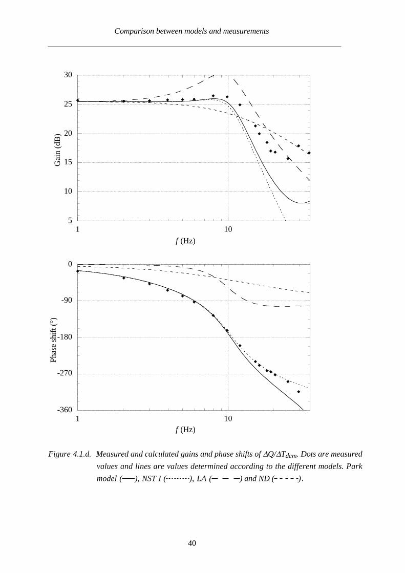
Figure 4.1.d. Measured and calculated gains and phase shifts of ∆Q/∆Tdcm. Dots are measured
values and lines are values determined according to the different models. Park
model ( ), NST I ( ), LA ( ) and ND ( ).

Comparison between models and measurements
41
-35
-30
-25
-20
-15
-10
-5
1 10
Gai
n (d
B)
f (Hz)
-180
-135
-90
-45
0
1 10
Phas
e sh
ift (
°)
f (Hz)
Figure 4.1.e. Measured and calculated gains and phase shifts of ∆Is/∆Tdcm. Dots are measured
values and lines are values determined according to the different models. Park
model ( ), NST I ( ), LA ( ) and ND ( ).

Comparison between models and measurements
42
The measured electrodynamical torque, electric power and stator current responses agree well
with the values predicted by the Park model, while the reactive power response agrees only up
to a perturbation frequency of 10 Hz. The rotor speed response has a 10 % discrepancy above
a perturbation frequency of 5 Hz. Similar observations were made when the machine was
operating as generator. The dominating eigenfrequency of the 15 kW machine operating at 288
V and 43.5 Hz with a moment of inertia of 0.45 kgm2, 10 Hz, is visible in Figures 4.1.a-e.
A first-order model is possible to use up to a perturbation frequency of about 3 Hz if an error
of 10 % is the maximum allowed. This frequency is a third of the dominating eigenfrequency
of the 15 kW machine. The rotor speed, electrodynamical torque and electric power responses
predicted by the LA-model have a maximum error of about 10 % compared to the Park model.
Finally, the NST I-model is almost as good as the Park model.
In Table 4.1 the error ε defined by (4.1) is presented for the different models and different
outputs. It can be noted that the NST III-model predicts excellent characteristics of the
induction machine when the responses to shaft torque disturbances is to be determined. It can
further be observed that the NSR-model has a larger rotor speed response error than the LA-
model. In Figure 4.2 the calculated gains of ∆Ωm/∆Ts predicted by the NSR-model and LA-
model are compared to the one obtained using the Park model.
Table 4.1. Error values of the simplified models.
∆Te/∆Tdcm ∆Ωm/∆Tdcm ∆Pe/∆Tdcm ∆Q/∆Tdcm ∆Is/∆Tdcm
NST III-model 0.0013 0.0010 0.0014 0.0010 0.0022
NST I-model 0.0089 0.0083 0.0089 0.0196 0.0094
NSR-model 0.019 0.067
LA-model 0.0233 0.034 0.021 0.42 0.078
ND-model 0.17 0.25 0.17 0.35 0.19
LD-model 0.17 0.28 0.21 0.37 0.24

Comparison between models and measurements
43
-40
-35
-30
-25
-20
1 10
Park modelNSR-modelLA-model
Gai
n (d
B)
f (Hz)
Figure 4.2. Calculated gain of ∆Ωm/∆Ts for the Park model and the two second-order models.
In Figure 4.2 it can be observed that the NSR-model predicts a rather good rotor speed
response around the eigenfrequency of the machine. The reason for the high error value in
Table 4.1 can be found in the lower frequency region, where the NSR-model does not predict a
correct steady-state response. However, keeping in mind that this model is very simple, it
provides good characteristics of the induction machine, suitable for many applications.
In Figure 4.3 the calculated gains of ∆Ωm/∆Ts predicted by the linear and non-linear first-order
models are compared to the one obtained using the Park model. Again it can be observed from
the figure that the dynamics of the models are quite similar but the linear model fails to predict a
correct steady-state response.

Comparison between models and measurements
44
Gai
n (d
B)
-40
-35
-30
-25
-20
1 10
Park modelLD-modelND-model
f (Hz)
Figure 4.3. Calculated gain of ∆Ωm/∆Ts for the Park model and the first-order models.
4.2 Supply frequency perturbation
The measured and calculated responses to perturbations in the supply frequency are shown in
Figs. 4.4.a-e. Measured and calculated results are presented only for motor operation since the
induction machine response to perturbations in the supply frequency does not depend much on
the static shaft torque.

Comparison between models and measurements
45
-5
0
5
10
15
20
25
1 10
Phas
e sh
ift (
°)
f (Hz)
-180
-135
-90
-45
0
45
90
1 10
Phas
e sh
ift (
°)
f (Hz)
Figure 4.4.a. Measured and calculated gains and phase shifts of ∆Te/∆ωs. Dots are measured
values and lines are values determined according to the different models. Park
model ( ), NST I ( ), LA ( ) and ND ( ).

Comparison between models and measurements
46
-30
-25
-20
-15
-10
-5
1 10
Gai
n (d
B)
f (Hz)
-270
-225
-180
-135
-90
-45
0
1 10
Phas
e sh
ift (
°)
f (Hz)
Figure 4.4.b. Measured and calculated gains and phase shifts of ∆Ωm/∆ωs. Dots are measured
values and lines are values determined according to the different models. Park
model ( ), NST I ( ), LA ( ) and ND ( ).

Comparison between models and measurements
47
35
40
45
50
55
60
65
1 10
Gai
n (d
B)
f (Hz)
-180
-135
-90
-45
0
45
90
1 10
Phas
e sh
ift (
°)
f (Hz)
Figure 4.4.c. Measured and calculated gains and phase shifts of ∆Pe/∆ωs. Dots are measured
values and lines are values determined according to the different models. Park
model ( ), NST I ( ), LA ( ) and ND ( ).

Comparison between models and measurements
48
20
30
40
50
60
1 10
Gai
n (d
B)
f (Hz)
-360
-315
-270
-225
-180
-135
-90
1 10
Phas
e sh
ift (
°)
f (Hz)
Figure 4.4.d. Measured and calculated gains and phase shifts of ∆Q/∆ωs. Dots are measured
values and lines are values determined according to the different models. Park
model ( ), NST I ( ), LA ( ) and ND ( ).

Comparison between models and measurements
49
-20
-15
-10
-5
0
5
10
15
1 10
Gai
n (d
B)
f (Hz)
-180
-135
-90
-45
0
45
90
1 10
Phas
e sh
ift (
°)
f (Hz)
Figure 4.4.e. Measured and calculated gains and phase shifts of ∆Is/∆ωs. Dots are measured
values and lines are values determined according to the different models. Park
model ( ), NST I ( ), LA ( ) and ND ( ).

Comparison between models and measurements
50
The measured responses to supply frequency perturbations agree well with those predicted by
the Park model up to a perturbation frequency of 15 Hz. The predicted rotor speed response is
somewhat higher than the measured one, for perturbations frequencies between 5 and 10 Hz,
but the discrepancy is smaller than in the case where the response to torque perturbations was
investigated.
At low frequencies, the different models predict similar induction machine responses, but at a
frequency above a few Hz, the discrepancy between the first-order model and the Park model
becomes significant. The approximation of an upper perturbation frequency of 3 Hz for the
first-order model is useful also as an upper limit in determining the responses to supply
frequency perturbations.
The NST I-model predicts the responses to supply frequency perturbations rather well. The
discrepancy compared to the Park model grows as the perturbation frequency increases and
reaches 10 % at the dominating eigenfrequency. However, the discrepancy is larger in the
prediction of the reactive power and stator current responses.
The LA-model predicts similar rotor speed, electrodynamical torque and electric power
responses as the NST I-model, while the stator current and reactive power responses are much
less accurate.
The error values determined according to (4.1) are presented in Table 4.2. It can be observed
that the linear NSR-model predicts similar rotor speed and electrodynamical torque responses
to supply frequency perturbations as the LA-model, in fact, the error values are even lower for
the NSR-model. Moreover, it can be seen that the NST III-model predicts the transfer function
∆Ωm/∆ωs excellently while the prediction of the other responses to the supply frequency
perturbations using the NST III-model is less good. In Figure 4.5 the magnitudes of ∆Te/∆ωs
is presented for the Park model and the two NST-models.
Table 4.2. Error values of the simplified models.
∆Te/∆ωs ∆Ωm/∆ωs ∆Pe/∆ωs ∆Q/∆ωs ∆Is/∆ωs
NST III-model 0.053 0.0027 0.051 0.056 0.047
NST I-model 0.019 0.019 0.021 0.033 0.020
NSR-model 0.027 0.027
LA-model 0.036 0.036 0.040 0.92 0.36
ND-model 0.18 0.18 0.18 0.87 0.43
LD-model 0.18 0.18 0.22 0.82 0.34

Comparison between models and measurements
51
Gai
n (d
B)
-5
0
5
10
15
20
25
1 10
Park modelNST INST III
f (Hz)
Figure 4.5. Calculated gain of ∆Te/∆ωs for the Park model and the NST-models.
The NST III-model predicts an excellent electrodynamical torque response around the
eigenfrequency but it predicts 6 % too high an electrodynamic torque response to perturbation
frequencies below 7 Hz, which causes the large error value in Table 4.2.
4.3 Perturbations in the supply voltage magnitude
The responses to voltage magnitude perturbations depend on the steady-state shaft torque of the
machine. In Figures 4.6.a-e and Figures 4.7.a-e the responses to voltage magnitude
perturbations are presented at generator and motor operation, respectively. In the cases where
the effect of saturation and iron losses are of importance, results calculated taking these effects
into account are also presented.

Comparison between models and measurements
52
-50
-40
-30
-20
-10
0
10
20
1 10
Gai
n (d
B)
f (Hz)
-360
-270
-180
-90
0
1 10
Phas
e sh
ift (
°)
f (Hz)
Figure 4.6.a. Measured and calculated gains and phase shifts of ∆Te/∆U. Dots are measured
values and lines are values determined according to the different models. Park
model ( ), NST I ( ), LA ( ) and ND ( ).

Comparison between models and measurements
53
-55
-50
-45
-40
-35
-30
-25
-20
1 10
Gai
n (d
B)
NST III-model
f (Hz)
-90
0
90
180
270
1 10
Phas
e sh
ift (
°)
NST III-model
f (Hz)
Figure 4.6.b. Measured and calculated gains and phase shifts of ∆Ωm/∆U. Dots are measured
values and lines are values determined according to the different models. Park
model ( ), NST III ( ), NST I ( ), LA ( ) and ND ( ).

Comparison between models and measurements
54
-20
-10
0
10
20
30
40
50
60
1 10
Gai
n (d
B)
Saturation and ironlosses included
f (Hz)
-360
-270
-180
-90
0
1 10
Phas
e sh
ift (
°)
Saturation and ironlosses included
f (Hz)
Figure 4.6.c. Measured and calculated gains and phase shifts of ∆Pe/∆U. Dots are measured
values and lines are values determined according to the different models. Park
model ( ), Two-axis model with saturation and iron losses considered ( ),
NST I ( ), LA ( ) and ND ( ).

Comparison between models and measurements
55
30
35
40
45
50
55
1 10
Gai
n (d
B)
Saturation and ironlosses included
f (Hz)
-45
0
45
90
1 10
Phas
e sh
ift (
°)
Saturation and ironlosses included
f (Hz)
Figure 4.6.d. Measured and calculated gains and phase shifts of ∆Q/∆U. Dots are measured
values and lines are values determined according to the different models. Park
model ( ), Two-axis model with saturation and iron losses considered ( ),
NST I ( ), LA ( ) and ND ( ).
Comparison between models and measurements
56
-60
-50
-40
-30
-20
-10
0
10
1 10
Gai
n (d
B)
Saturation and ironlosses included
f (Hz)
-90
-45
0
45
90
135
1 10
Phas
e sh
ift (
°)
Saturation and ironlosses included
f (Hz)
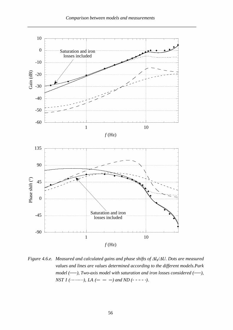
Figure 4.6.e. Measured and calculated gains and phase shifts of ∆Is/∆U. Dots are measured
values and lines are values determined according to the different models.Park
model ( ), Two-axis model with saturation and iron losses considered ( ),
NST I ( ), LA ( ) and ND ( ).

Comparison between models and measurements
57
-50
-40
-30
-20
-10
0
10
20
1 10
Gai
n (d
B)
f (Hz)
-45
0
45
90
135
180
1 10
Phas
e sh
ift (
°)
f (Hz)
Figure 4.7.a. Measured and calculated gains and phase shifts of ∆Te/∆U. Dots are measured
values and lines are values determined according to the different models. Park
model ( ), NST I ( ), LA ( ) and ND ( ).

Comparison between models and measurements
58
-50
-45
-40
-35
-30
-25
-20
1 10
Gai
n (d
B)
NST III-model
f (Hz)
-90
-45
0
45
90
1 10
Phas
e sh
ift (
°)
NST III-model
f (Hz)
Figure 4.7.b. Measured and calculated gains and phase shifts of ∆Ωm/∆U. Dots are measured
values and lines are values determined according to the different models. Park
model ( ), NST III ( ), NST I ( ), LA ( ) and ND ( ).

Comparison between models and measurements
59
-10
0
10
20
30
40
50
60
1 10
Gai
n (d
B)
Saturation and ironlosses included
f (Hz)
0
45
90
135
180
1 10
Gai
n (d
B)
Saturation and ironlosses included
f (Hz)
Figure 4.7.c. Measured and calculated gains and phase shifts of ∆Pe/∆U. Dots are measured
values and lines are values determined according to the different models. Park
model ( ), Two-axis model with saturation and iron losses considered ( ),
NST I ( ), LA ( ) and ND ( ).

Comparison between models and measurements
60
30
35
40
45
50
55
60
1 10
Gai
n (d
B) Saturation and iron
losses included
f (Hz)
-45
0
45
1 10
Phas
e sh
ift (
°)
Saturation and ironlosses included
f (Hz)
Figure 4.7.d. Measured and calculated gains and phase shifts of ∆Q/∆U. Dots are measured
values and lines are values determined according to the different models. Park
model ( ), Two-axis model with saturation and iron losses considered ( ),
NST I ( ), LA ( ) and ND ( ).
Comparison between models and measurements
61
-40
-30
-20
-10
0
10
1 10
Gai
n (d
B)
Saturation and ironlosses included
f (Hz)
0
45
90
135
180
1 10
Phas
e sh
ift (
°)
Saturation and ironlosses included
f (Hz)
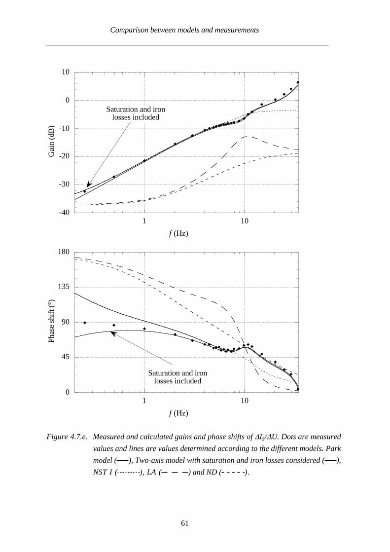
Figure 4.7.e. Measured and calculated gains and phase shifts of ∆Is/∆U. Dots are measured
values and lines are values determined according to the different models. Park
model ( ), Two-axis model with saturation and iron losses considered ( ),
NST I ( ), LA ( ) and ND ( ).

Comparison between models and measurements
62
The standard Park model predicts the rotor speed and electrodynamical torque responses rather
well but it is necessary to consider the iron losses when the electric power and stator current
responses are determined.
The error values determined according to (4.1) are presented in Table 4.3. Since the
performance of the models varies with the operating point, when the machine is subjected to
voltage magnitude perturbations, the average values of the error at motor and generator
operation are presented.
Table 4.3. Error values of the simplified models.
∆Te/∆U ∆Ωm/∆U ∆Pe/∆U ∆Q/∆U ∆Is/∆U
NST III-model 1.3 0.020 2.2 0.038 0.15
NST I-model 0.21 0.21 0.36 0.027 0.053
LA-model 0.46 0.46 0.97 0.52 0.86
ND-model 0.30 0.30 0.81 0.51 0.86
The ND-model predicts the rotor speed and electrodynamical torque responses rather well up to
a perturbation frequency of about 2 Hz. The upper frequency limit below which the first-order
model can predict accurate responses thus is somewhat lower in the voltage magnitude
perturbation case than in the torque or supply frequency perturbation case. The LA-model is
approximately as useful as a first-order model in predicting the responses to voltage magnitude
perturbations.
The NST I-model is not much better than the LA-model in determining the rotor speed,
electrodynamical torque and electric power responses to voltage magnitude perturbations.
However, the stator current and reactive power responses predicted by the NST I-model are
much better compared to the ones obtained using the LA-model. The NST III-model predicts an
excellent rotor speed response while it do not predict the electrodynamical torque, electric
power and stator current responses as well as the NST I-model. This fact demonstrates that it is
dangerous to validate a model based on only one transfer function as Wasynczuk et al. (1985)
did. In Figure 4.8 the magnitudes of ∆Te/∆U is presented in motor operation for the Park model
and the two NST models.
Again, the observation can be made that the values obtained using the NST III-model differ
from those obtained using the Park model for very low perturbation frequencies, which causes
the large error in Table 4.3. The reason for this error is the fact that the derivatives of the input
signals are needed to predict a correct answer.

Comparison between models and measurements
63
Gai
n (d
B)
-40
-30
-20
-10
0
10
20
1 10
Park modelNST I-modelNST III-model
f (Hz)
Figure 4.8. Calculated gain of ∆Te/∆U for the Park model and the NST-models.
4.4 Response of a two-machine group
There are two methods of reducing the order of a multi-machine system: reduction of induction
machine groups to single-unit equivalents, i.e. aggregate models, and simplified representation
of each machine. If the interior signals are of no interest, the model order of a multi-machine
system can be reduced by replacing the machines with one equivalent machine, i.e. an
aggregate model. However, if the interior signals are of interest, the approach of simplified
representation of each machine must be used.
When the response of a two-machine group was investigated, an additional converter-fed dc
machine-induction machine set-up was used, identical to the one described in Chapter 3. The
two induction machines were connected to the forced-commutated converter via a resistance,
Rl = 0.72 Ω, and an inductance, Ll = 2 mH. Figure 4.9 shows the set-up consisting of the
line impedances and the induction machines.

Comparison between models and measurements
64
U
Ugrid
LlRl
Machine 1
Machine 2
Figure 4.9. The investigated two-machine system.
The two-machine system was modelled in the following way: The two machines, represented
by Park models/NST-models/LA-models/ND-models were connected to a local grid, which
was connected to an infinite bus via a line inductance and resistance. The dynamic influence of
the line inductance was taken into account. In power system analysis programs, the dynamic
influence of the line inductances is usually neglected, i.e. the line impedance current derivatives
are neglected.
If the derivatives of the line impedance currents were neglected, the maximum magnitudes of
the transfer functions were typically reduced by 10 % for the two-machine systems based on
the Park models and NST I-models. For the LA-model and ND-model, the neglection of the
derivatives had a very small influence. Figure 4.10 presents the calculated magnitudes of the
transfer function ∆Te1/∆Tdcm1 using the Park model-based two-machine system with and
without the dynamics of the line impedance incorporated.
The line resistance used here is 0.72 Ω, i.e. 0.16 p.u. if 288 V and 64 A are used as the base
voltage and base current, respectively. If the machines operate at rated current, the losses in the
line resistance will be 3 kW, i.e., 10 % of the rated power of the two machines. The line
inductance was 2 mH (j0.55Ω). This gives a short-circuit capacity of 90 kVA at the machines,
i.e., only three times the rating of the two machines. This was done in order to obtain a strong
interaction between the induction machines.

Comparison between models and measurements
65
-10
-5
0
5
10
1 10
Gai
n (d
B)
Figure 4.10. Calculated gains of ∆Te1/∆Tdcm1. Solid line represents the calculations performed
taking the dynamic influence of the line impedance into account and the dashed
curve represents the calculations where the dynamic influence of the line
impedance has been ignored.
The high value of the line impedance led to an unexpected problem: the simulation of the two-
machine system using the NST-models to represent the machines did not work unless the line
impedance was reduced by 30 %. However, a model producing very similar results was used
instead: A new sixth-order model was derived starting from the equations of the whole two-
machine system which is a tenth-order system. The procedure suggested by Wasynczuk et al.
(1985) was then applied to this system. All four stator flux linkage transients were neglected
resulting in a sixth-order model. This model and a two-machine model with single-machine
NST-models produced very similar responses when a system with only one third of the used
line impedance was investigated.
In Figures 4.11-4.13, the responses predicted by the different models are presented together
with the measured ones for some selected responses to torque, supply frequency and voltage
magnitude perturbations.
Machine 1 is operating as motor and Machine 2 is operating as generator, loaded and driven by
a shaft torque of 35 Nm. A shaft torque of 35 Nm at the used voltage level and supply
frequency corresponds to a slip of approximately one third of the rated value.
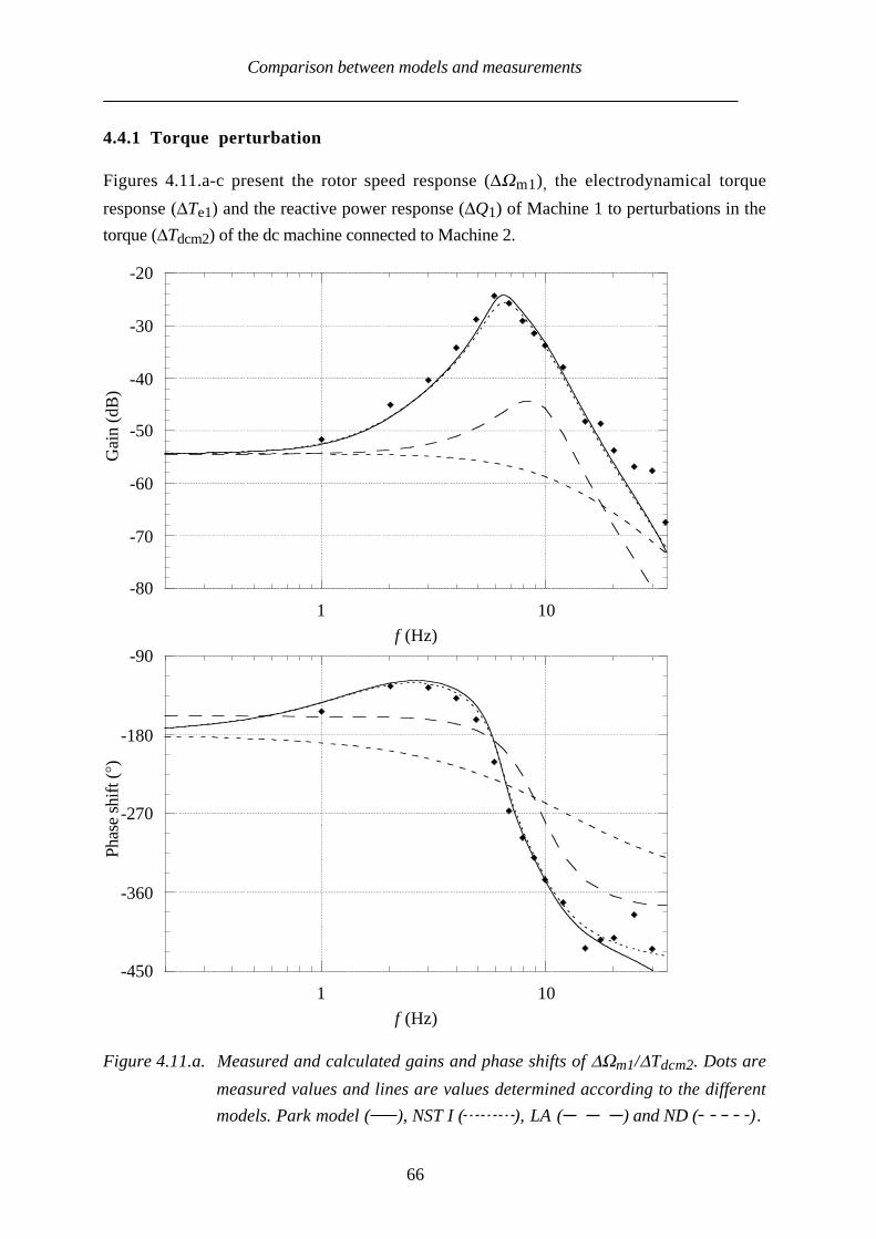
Comparison between models and measurements
66
4.4.1 Torque perturbation
Figures 4.11.a-c present the rotor speed response (∆Ωm1), the electrodynamical torque
response (∆Te1) and the reactive power response (∆Q1) of Machine 1 to perturbations in the
torque (∆Tdcm2) of the dc machine connected to Machine 2.
-80
-70
-60
-50
-40
-30
-20
1 10
Gai
n (d
B)
f (Hz)
-450
-360
-270
-180
-90
1 10
Phas
e sh
ift (
°)
f (Hz)
Figure 4.11.a. Measured and calculated gains and phase shifts of ∆Ωm1/∆Tdcm2. Dots are
measured values and lines are values determined according to the different
models. Park model ( ), NST I ( ), LA ( ) and ND ( ).

Comparison between models and measurements
67
-60
-50
-40
-30
-20
-10
0
10
1 10
Gai
n (d
B)
f (Hz)
-360
-270
-180
-90
0
1 10
Phas
e sh
ift (
°)
f (Hz)
Figure 4.11.b. Measured and calculated gains and phase shifts of ∆Te1/∆Tdcm2. Dots are
measured values and lines are values determined according to the different
models. Park model ( ), NST I ( ), LA ( ) and ND ( ).

Comparison between models and measurements
68
-10
0
10
20
30
40
1 10
Gai
n (d
B)
f (Hz)
-540
-450
-360
-270
-180
-90
1 10
Phas
e sh
ift (
°)
f (Hz)
Figure 4.11.c. Measured and calculated gains and phase shifts of ∆Q1/∆Tdcm2. Dots are
measured values and lines are values determined according to the different
models. Park model ( ), NST I ( ), LA ( ) and ND ( ).
The values determined using the Park model coincide well with the measured ones. The NST-
model predicts similar results as the Park model. The LA-model and the ND-model can be used
to predict the induction machine responses to shaft torque perturbations for perturbation
frequencies below 1-2 Hz.

Comparison between models and measurements
69
4.4.2 Supply frequency perturbation
Figures 4.12.a-c present the rotor speed response of Machine 1 (∆Ωm1), the electrodynamical
torque response of Machine 2 (∆Te2) and the active power response of machine two (∆P2) to
perturbations in the supply frequency (∆ωs).
Gai
n (d
B)
-40
-30
-20
-10
0
1 10f (Hz)
-270
-180
-90
0
90
1 10
Phas
e sh
ift (
°)
f (Hz)
Figure 4.12.a. Measured and calculated gains and phase shifts of ∆Ωm1/∆ωs. Dots are
measured values and lines are values determined according to the different
models. Park model ( ), NST I ( ), LA ( ) and ND ( ).

Comparison between models and measurements
70
-20
-10
0
10
20
30
1 10
Gai
n (d
B)
f (Hz)
-180
-90
0
90
1 10
Phas
e sh
ift (
°)
f (Hz)
Figure 4.12.b. Measured and calculated gains and phase shifts of ∆Te2/∆ωs. Dots are
measured values and lines are values determined according to the different
models. Park model ( ), NST I ( ), LA ( ) and ND ( ).

Comparison between models and measurements
71
20
30
40
50
60
70
1 10
Gai
n (d
B)
f (Hz)
-180
-90
0
90
180
1 10
Phas
e sh
ift (
°)
f (Hz)
Figure 4.12.c. Measured and calculated gains and phase shifts of ∆P2/∆ωs. Dots are
measured values and lines are values determined according to the different
models. Park model ( ), NST I ( ), LA ( ) and ND ( ).
The Park model calculations agree well with the measured values. The NST-model predicts
almost the same result as the Park model. Again, the LA-model and the ND-model is useful up
to a perturbation frequency of about 1-2 Hz.

Comparison between models and measurements
72
4.4.3 Voltage magnitude perturbation
Figures 4.13.a-c present the rotor speed responses of machines one and two, as well as the
local grid voltage response (∆Ugrid) to perturbations in the voltage magnitude (∆U).
-60
-50
-40
-30
-20
1 10
Gai
n (d
B)
f (Hz)
-180
-135
-90
-45
0
45
90
135
1 10
Phas
e sh
ift (
°)
f (Hz)
Figure 4.13.a. Measured and calculated gains and phase shifts of Ωm1/∆U. Dots are measured
values and lines are values determined according to the different models. Park
model ( ), NST I ( ), LA ( ) and ND ( ).
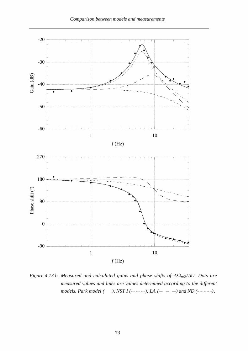
Comparison between models and measurements
73
-60
-50
-40
-30
-20
1 10
Gai
n (d
B)
f (Hz)
-90
0
90
180
270
1 10
Phas
e sh
ift (
°)
f (Hz)
Figure 4.13.b. Measured and calculated gains and phase shifts of ∆Ωm2/∆U. Dots are
measured values and lines are values determined according to the different
models. Park model ( ), NST I ( ), LA ( ) and ND ( ).

Comparison between models and measurements
74
-10
-8
-6
-4
-2
0
1 10
Gai
n (d
B)
f (Hz)
-50
-40
-30
-20
-10
0
10
1 10
Phas
e sh
ift (
°)
f (Hz)
Figure 4.13.c. Measured and calculated gains and phase shifts of ∆Ugrid/∆U. Dots are
measured values and lines are values determined according to the different
models. Park model ( ), NST I ( ), LA ( ) and ND ( ).
The values determined using the Park model and the NST-model coincide well with the
measured ones. The only exception is that the iron losses should be taken into account to obtain
a correct active power response to very low-frequency voltage magnitude perturbations, below
approximately 3 Hz for the investigated system. The LA-model is as useful as the ND-model,
i.e. valid up to a perturbation frequency of about 1 Hz.

Some aspects on induction machine dynamics
75
5 SOME ASPECTS ON INDUCTION MACHINE DYNAMICS
The purpose of this chapter is to discuss different aspects that influence the induction machine
dynamics, such as different operating points, disturbance magnitude, skin effect, iron losses,
main flux saturation, line impedance and variable frequency.
The magnitude of ∆Te/∆Ts is typically shown in this chapter in order to reduce the number of
cases presented. However, other transfer functions are also shown when they are of interest.
5.1 Steady-state shaft torque
In a linear system, the gain is always independent of the operating point. Since the induction
machine is a non-linear system this is not the case. However, the steady-state shaft torque is
not of such great importance in the steady-state operating region of the inductance machine, as
will be shown in this section. The calculations in this section are performed on the 15 kW
machine at a voltage level of 400 V and at a supply frequency of 50 Hz using the Park model.
Within the normal operating region of the machine, the electrodynamical torque response to
shaft torque perturbations is only slightly influenced by the static shaft torque (Kovacs 1984).
Figure 5.1 presents the calculated magnitudes ∆Te/∆Ts at no load operation and at rated motor
operation. The reason for selecting these operating points is that the lowest damping and the
highest damping occur close to no load operation and in rated motor operation, respectively.
Gai
n (d
B)
-10
-5
0
5
10
1 10
no load operation
rated motor operation
f (Hz)
Figure 5.1. Calculated magnitudes of ∆Te/∆Ts. The machine is operating as motor loaded by
rated torque and at no load. Temperature variations are not taken into account.

Some aspects on induction machine dynamics
76
As can be noted from the figure, the discrepancy between the ratios ∆Te/∆Ts for the two
different cases is only notable for perturbation frequencies around and above the
eigenfrequency, where it is about 10 %. In the normal steady-state operating region it is more
important that the damping is improved as the temperature in the machine increases. As the
temperature raises, the stator resistance increases, which leads to reduced damping, and the
rotor resistance also grows leading to improved damping. The total effect is that the damping
increases as the temperature raises.
In Figure 5.2 the calculated ratios of ∆Te/∆Ts are presented for some operating points taking
temperature variations into account. As can be noted the maximum magnitude of ∆Te/∆Ts is 50
% lower at rated load than in the case where the machine is cold and operating at no load.
Gai
n (d
B)
-5
0
5
10
1 10
no load, cold machine
no load
2/3 of rated load
rated load
f (Hz)
Figure 5.2. Calculated magnitudes of ∆Te/∆Ts at some operating points with temperature
variations taken into account.
The induction machine response to frequency perturbations also varies only slightly in the
normal steady-state operating region, if temperature changes are not taken into account. The
stator current and especially the reactive power responses to shaft torque and supply frequency
perturbations, however, depend strongly on the operating point, even if temperature changes
are not accounted for.
The response to perturbations in the magnitude of the supply voltage depends strongly on the
static shaft torque even if temperature changes are not taken into account. Figure 5.3 presents
the calculated rotor speed response to perturbations in the magnitude of the supply voltage
when the machine is operating in generator and in motor operation, driven and loaded by rated
torque.

Some aspects on induction machine dynamics
77
Gai
n (d
B)
-40
-20
0
1 10
Phas
e sh
ift (
°)
-90
0
90
180
1 10f (Hz) f (Hz)
Figure 5.3. Magnitudes and arguments of ∆Ωm/∆U in motor (solid curve) and in generator
operation (dashed curve).
In motor operation there exists an anti-resonance at 7 Hz which does not occur in generator
operation. If small-signal analysis is applied on the machine operating as motor, a complex-
conjugated double-zero can be observed which corresponds to the anti-resonance. In generator
operation no complex-conjugated double-zero exists, but instead a zero can be found in the
right half of the s-plane making the induction machine in this case to a mixed-phase system
(Proakis & Manolakis 1988). This means that if the voltage is increased in generator operation,
the immediate rotor speed response will be opposite to the final change.
5.2 Disturbance magnitude
In a linear system the gain is always independent of the perturbation magnitude. However, in a
non-linear system this is not the case. For instance, if the induction machine is subjected to a
large shaft torque disturbance, this will cause the machine to pass the pull-out point. An
important question is thus: how large input perturbation magnitudes can be tolerated before the
results of a small-signal analysis become inaccurate?
By applying small signal analysis on (2.4), we get
Te0 + ∆Te = p Im(Ψs0*is0 + Ψs0
*∆is + ∆Ψs*is0 + ∆Ψs
*∆is) (5.1)
and with the steady-state solution subtracted
∆Te = p Im(Ψs0*∆is + ∆Ψs
*is0 + ∆Ψs*∆is) (5.2)

Some aspects on induction machine dynamics
78
The last term in (5.2), a product of small disturbances, is neglected in small signal analysis,
which finally gives
∆Te = p Im(Ψs0*∆is + ∆Ψs
*is0) (5.3)
As a large pulsation in the supply voltage magnitude, 20% of the nominal grid voltage was
selected and 3 % was selected as a small perturbation magnitude. The reason for selecting 3 %
is that this is the highest voltage magnitude perturbation allowed by IEC 555-3 for extremely
low-frequency voltage perturbations. In fact, for perturbation frequencies between 1 and
30 Hz, the limit is less than 1 %. In Figure 5.4 the magnitudes of ∆Ωm/∆U for the two
perturbation magnitudes are presented. The machine is operating at 400 V and 50 Hz as motor
loaded by rated torque. Again, small-signal analysis was applied but the results did not differ
from those obtained using the small perturbation magnitude and accordingly the small-signal
results are not presented.
Gai
n (d
B)
-40
-30
-20
-10
0
1 10 f (Hz)
Figure 5.4. Calculated magnitudes of ∆Ωm/∆U with different perturbation magnitudes. The
dashed curve represents results obtained using a small perturbation magnitude and
the solid one represents results using a large perturbation magnitude.
We have a maximum discrepancy of 10 %, which in this case is visible around the anti-
resonance frequency, 7 Hz. Figure 5.5 illustrates the electrodynamical responses to a 7 Hz
perturbation in the magnitude of the supply voltage of ∆U = 12 V and ∆U = 80 V. A
component at a frequency twice the applied one is clearly visible in Figure 5.6. Neglecting the
last term in (5.2) works well in the case where the disturbance is 8 V, but in the second case
this term is too large to be neglected.

Some aspects on induction machine dynamics
79
∆Te/
∆U
(Nm
/V)
-0.03
-0.02
-0.01
0
0.01
0.02
0.03
0 0.1 0.2 0.3t (s)
Figure 5.5. Torque response to a small (dashed curve) and a large (solid curve) perturbation
in the supply voltage magnitude.
A calculated example is presented in Figure 5.6, in which a large (100 % of rated torque, peak
to peak) and a small (10 % of rated torque) shaft torque perturbation are applied on the 15 kW
machine operating as motor at rated torque (U = 400 V and f = 50 Hz). Calculations were also
performed using a model linearized at the investigated operating point, but since the results
coincided with the results obtained using the small perturbation magnitude, the small-signal
analysis result is not presented.
Gai
n (d
B)
-10
-5
0
5
10
1 10 f (Hz)
Figure 5.6. Calculated magnitudes of ∆Te/∆Ts with different perturbation magnitudes. The
dashed curve represents results obtained using a small perturbation magnitude and
the solid one represents results using a large perturbation magnitude.

Some aspects on induction machine dynamics
80
Although the point (in the steady-state operating region) is reached where the non-linearity of
the machine is as most important the difference in the magnitude ∆Te/∆Ts is detectable only
around the dominating eigenfrequency, where it is about 10 %. In generator operation, where
the slope of the steady-state torque-speed curve decreases less, the influence is smaller.
The magnitude of a supply frequency perturbation can be up to about 5 Hz before the results
differ more than 10 % from the results obtained using small-signal analysis. Sometimes it is of
greater interest to define the allowed phase deviation instead of the allowed frequency variation.
In order to obtain a result which deviates less than 10 % from the small-signal analysis, the
phase perturbation must be below 10°.
5.3 Main flux saturation
As the flux in the machine increases, the value of the magnetizing inductance decreases due to
saturation. This is of no importance below rated flux for the investigated 15 kW machine and at
rated flux of little importance. The saturation can be taken into account for steady-state
purposes by adjusting only the magnetizing inductance. In order to take the dynamic effects of
the main flux saturation into consideration, the approach in Section 2.3 can be used.
Figure 5.7 presents the calculated magnitudes of ∆Te/∆Ts with dynamic saturation effects as
well as without saturation effects considered, not even a steady-state correction of the
magnetizing inductance. The applied voltage is 276 V and the supply frequency is 30 Hz,
which corresponds to a flux increase of 20 % compared to the nominal one (380 V and 50 Hz).
The value of the magnetizing inductance is in this case only 65 % of the nominal one.
Gai
n (d
B)
-10
0
10
1 10f (Hz)
Figure 5.7. Calculated magnitudes of ∆Te/∆Ts with saturation effects taken into account,
dashed curve, and without effects of saturation taken into account, solid curve.

Some aspects on induction machine dynamics
81
From Figure 5.7 it can be noted that the peak gain of ∆Te/∆Ts is reduced by about 10 % when
the saturation is taken into account. However, if the same magnetizing inductance, i.e. the
saturated one, is used in both calculations, the difference between the two calculations is
reduced to almost nothing.
Melkebeek (1980, 1983) measured and calculated the rotor speed response to voltage
magnitude perturbations at no load, at frequencies around the resonance frequency, and found
that the saturation reduced the magnitude of the rotor speed response substantially. For a
2.2 kW machine at a nominal flux level, he found a 50 % reduction of ∆Ωm/∆U at the
resonance frequency compared to the case where the flux level of the machine was about 50 %
of the nominal one. Specially adapted rotors were used in the experiments.
For the 15 kW machine investigated, such an influence of saturation was not found. At
nominal flux levels, the calculated rotor speed response was the same with or without
saturation taken into account. At a flux level of 20 % higher than the nominal one, the
calculated peak magnitude of ∆Ωm/∆U was reduced by about 15 % due to saturation effects. If
the comparison was made with the same magnetizing inductance, i.e. only the dynamic
influence of the main flux saturation was investigated, the difference was reduced to about
3 %.
The strongest dynamic influence of the saturation was detected at very low-frequency
responses to voltage magnitude perturbations. (Melkebeek measured the rotor speed response
above about 10 Hz.) Figure 5.8 presents the measured and calculated magnitudes of ∆Te/∆U
and ∆Ωm/∆U with and without the dynamic effects of saturation taken into account. The same
magnetizing inductance is used for both cases. The applied voltage is 276 V and the supply
frequency is 30 Hz, i.e, the flux level used is 120 % of the nominal one.
A clear difference caused by the dynamic effect of the main flux saturation is visible in Figure
5.8. At the anti-resonance frequency, the rotor speed and electrodynamical torque responses to
voltage magnitude perturbations are three times higher when the dynamic effect of saturation is
accounted for compared to the case when only the steady-state effect of the saturation is taken
into account. Also the other responses to voltage magnitude perturbations of very low
frequencies are affected.

Some aspects on induction machine dynamics
82
Gai
n (d
B)
-40
-30
-20
-10
0
10
20
30
1 10
Gai
n (d
B)
-60
-50
-40
-30
-20
-10
0
1 10
f (Hz) f (Hz)
Figure 5.8. Calculated magnitudes of ∆Te/∆U (left) and ∆Ωm/∆U (right) with dynamic effects
of saturation taken into account, dashed curve, and without dynamic effects of
saturation taken into account, solid curve. Dots are measured values.
5.4 Skin effect
The rotor conductors of a cage induction machine are designed to have a higher resistance
increasing with higher rotor frequencies by utilizing the skin effect. Apart from the fact that the
starting torque is raised, the damping is also increased. Figure 5.9 presents the magnitudes of
∆Te/∆Ts with and without skin effect taken into account. The machine is operating at no load
and at U = 400 V and f = 50 Hz
Gai
n (d
B)
-10
-5
0
5
10
1 10
Without taking skin effect into account
Taking skin effect into account
f (Hz)
Figure 5.9. Calculated magnitudes of ∆Te/∆Ts with and without skin effect taken into account.

Some aspects on induction machine dynamics
83
At 18 Hz, which is the dominating resonance frequency of the 15 kW machine operating at
400 V and 50 Hz, the rotor resistance is increased by 10 %, and consequently the damping is
improved by 10 %. In a deep-bar rotor the increase of the rotor resistance will be larger. Meyer
(1976) found an increase of the damping by 20 % for a 3.1 MW machine at a rotor frequency
of 5 Hz, i.e. at the eigenfrequency of the induction machine investigated.
5.5 Inclusion of iron losses
Usually, the iron losses affect the dynamic behaviour of the machine very little. The only case
where the effect of iron losses is clearly visible is the electric power response to very low-
frequency perturbations in the voltage magnitude and supply frequency. Figure 5.10 presents
the magnitudes of ∆Pe/∆U when the machine is operating as generator driven by a shaft torque
of 70 Nm at U = 288 V and f = 43.5 Hz.
From Figure 5.10 it appears clearly that the iron losses have to be considered in order to
determine the magnitude of ∆Pe/∆U for perturbation frequencies below 3 Hz. However, it must
be pointed out that the electric power response magnitude is low for these low-frequency
perturbations.
Gai
n (d
B)
-20
-10
0
10
20
30
40
50
1 10
f (Hz)
Figure 5.10. Calculated and measured magnitudes of ∆Pe/∆U. Dots represent measured
values, dashed and solid lines represent calculations taking and not taking the
iron losses into account, respectively.
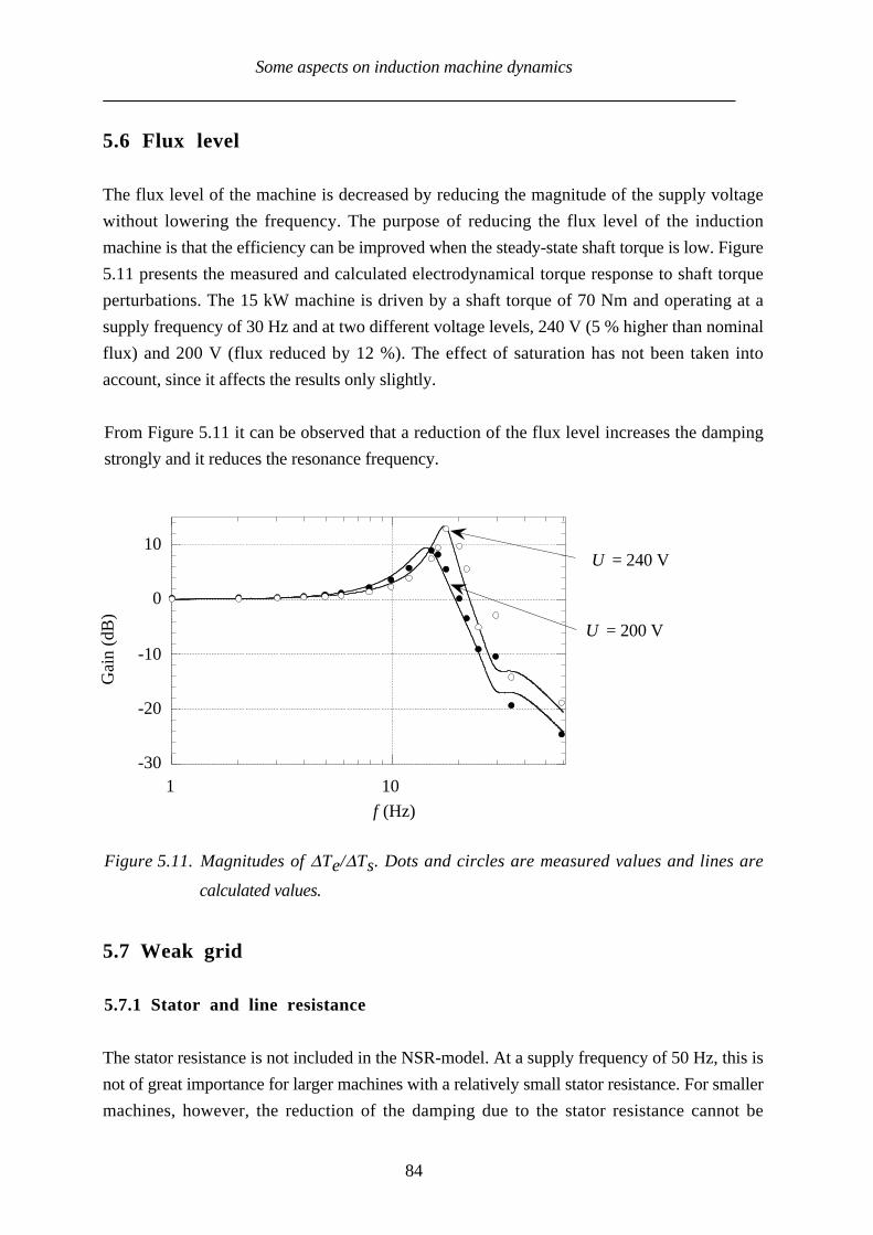
Some aspects on induction machine dynamics
84
5.6 Flux level
The flux level of the machine is decreased by reducing the magnitude of the supply voltage
without lowering the frequency. The purpose of reducing the flux level of the induction
machine is that the efficiency can be improved when the steady-state shaft torque is low. Figure
5.11 presents the measured and calculated electrodynamical torque response to shaft torque
perturbations. The 15 kW machine is driven by a shaft torque of 70 Nm and operating at a
supply frequency of 30 Hz and at two different voltage levels, 240 V (5 % higher than nominal
flux) and 200 V (flux reduced by 12 %). The effect of saturation has not been taken into
account, since it affects the results only slightly.
From Figure 5.11 it can be observed that a reduction of the flux level increases the damping
strongly and it reduces the resonance frequency.
Gai
n (d
B)
-30
-20
-10
0
10
1 10
U = 240 V
= 200 VU
f (Hz)
Figure 5.11. Magnitudes of ∆Te/∆Ts. Dots and circles are measured values and lines are
calculated values.
5.7 Weak grid
5.7.1 Stator and line resistance
The stator resistance is not included in the NSR-model. At a supply frequency of 50 Hz, this is
not of great importance for larger machines with a relatively small stator resistance. For smaller
machines, however, the reduction of the damping due to the stator resistance cannot be

Some aspects on induction machine dynamics
85
neglected. For the investigated 15 kW machine the damping predicted by the NSR-model is
20 % too low at 50 Hz and 400 V.
Even self-excited oscillations have been reported in cases where an extremely high additional
stator resistance has been used (Palit 1978, Kron & Lorenzon 1969). A series resistance must
accordingly be taken into account when the properties of the machine are determined. In Figure
5.12 the magnitudes of ∆Te/∆Ts are presented for some stator resistances. The machine is
operating as a generator driven by a shaft torque of 70 Nm, the voltage is 288 V and the supply
frequency is 43.5 Hz.
Gai
n (d
B)
-30
-20
-10
0
10
20
1 10
Nominal stator resistance
Stator resistanceincreased by 300 %
Stator resistanceincreased by 600 %
f (Hz)
Figure 5.12. Gain of the transfer function ∆Te/∆Ts with three different stator resistances. The
lines are calculated results performed according to the detailed model and the
dots, rhombuses and circles are measured values.
When the machine is fed from a converter, the resistance in the power switches, such as
transistors or GTOs, must be considered as the dynamic performance of the induction machine
is investigated. Another important feature of power switches is that they have a voltage drop,
which has the same effects as an additional stator resistance.
Increased stator resistance does not automatically lead to reduced damping. For low supply
frequencies the situation is usually the opposite. A growing stator resistance will always finally
lead to increased damping. Usually, the induction machine has a certain stator resistance value
where the damping reaches a minimum or even becomes negative. As the stator resistance
increases above this value, the damping is improved. For the 15 kW machine operating at 50
Hz and 400 V, the damping reaches a minimum for a stator resistance of 4.5 Ω, 25 times the

Some aspects on induction machine dynamics
86
rated value, with a damping ratio close to zero. At no load the machine will even be unstable.
Usually, the damping of the machine is improved as the inertia increases, but if we in this
example with a stator resistance of 4.5 Ω connect a load having an inertia equal to the inertia of
the machine, the machine will become even more unstable.
5.7.2 Line and leakage inductance
Additional line and stator leakage inductance mainly lead to a lowered resonance frequency.
Figure 5.13 shows the measured and calculated magnitudes of ∆Te/∆Ts for some stator leakage
inductances. The machine is operating as a generator driven by a shaft torque of 70 Nm. The
supply frequency is 43.5 Hz and the supply voltage is 288 V.
Gai
n (d
B)
-30
-20
-10
0
10
1 10
Nominal stator leakage inductance
Stator leakage inductanceincreased by 100 %
Stator leakage inductanceincreased by 200 %
f (Hz)
Figure 5.13. Magnitudes of ∆Te/∆Ts with different stator leakage inductances. The lines are
calculated results and the circles, dots and crosses are measured values.
5.8 Variable frequency
When an induction machine is driven in variable-speed operation, the voltage is usually
reduced in proportion to the frequency in order to keep a constant flux in the machine. If the
proportion between the supply voltage and supply frequency is kept constant, the NSR-model
(2.53) does not indicate that the dynamic behaviour should change as the supply frequency
varies. Figure 5.14 presents the measured and calculated magnitudes of ∆Te/∆Ts for three
different supply frequencies at the same flux level, 87 % of the nominal one. The machine is
operating as generator with a driving shaft torque of 70 Nm.

Some aspects on induction machine dynamics
87
Figure 5.14 shows that the supply frequency strongly affects the damping of the machine. It is
the influence of the stator resistance that leads to different dynamic behaviour as the supply
frequency varies. When the supply frequency is lowered, the stator resistance will be relatively
larger compared to the reactances of the machine.
Gai
n (d
B)
-30
-20
-10
0
10
20
1 10
supply frequency of 43.5 Hz
supply frequency of 30 Hz
supply frequency of 15 Hz
f (Hz)
Figure 5.14. Magnitudes of the transfer function ∆Te/∆Ts for some different supply
frequencies. Lines represent calculated values. Crosses, dots and circles show
measurements at 15, 30 and 43.5 Hz, respectively.
5.9 Influence of phase-compensating capacitors
To compensate for the reactive power needed by the induction machine, phase-compensating
capacitors can be installed at the machine. The low-frequency dynamic influence of the phase-
compensating capacitors is rather small. A minor influence can be observed depending on the
grid configuration, the capacitance and the static shaft torque of the machines. Generally, it can
be said that the damping is somewhat reduced, since the capacitors increase the voltage at the
induction machine.
In Figure 5.15 the measured and calculated magnitudes of ∆Ωm/∆Ts are presented with and
without capacitors of 300 µF per phase connected to the machine. The capacitance was chosen
to compensate the power factor to one at no load operation. An additional inductance of 2 mH
is also connected between the converter and the machine in both cases. The voltage at the
machine will otherwise be governed by the converter only, and the capacitors will have no
influence on the dynamic performance of the machine.

Some aspects on induction machine dynamics
88
The machine is operating as generator driven by a shaft torque of 70 Nm, the applied voltage is
288 V and the supply frequency is 43.5 Hz. The machine voltage is 286 V with capacitors and
274 V without. An additional calculation without capacitors was also performed at a higher
voltage level of 300 V. The voltage at the machine is in this case the same as when the 300 µF
capacitor was connected, i.e. 286 V.
From Figure 5.15 it can be observed that the rotor speed response is similar in the case where
capacitors were connected at the machine as when the applied voltage was increased and no
capacitors were used. The other responses are affected in a similar way. However, the reactive
power response to voltage magnitude perturbations has a more complicated pattern as phase-
compensating capacitors are connected, and depends both on the static shaft torque and the
capacitance.
Gai
n (d
B)
-35
-30
-25
-20
-15
1 10
Without capacitors
With capacitors
Measurements without capacitors
Measurements with capacitors
Calculations without capacitors butat a voltage level of 300 V
Figure 5.15. Magnitudes of ∆Ωm/∆Ts. Lines and crosses represent calculated values, and
circles and dots show measured values.
5.10 Non-stiff machine shaft
The purpose of deriving linear reduced order models of the induction machine is to simplify the
dynamic analysis. By using the LD-model and NSR-model it is possible to analyse a larger
system analytically, for instance the drive train of a wind turbine. Constant-speed wind
turbines often produce periodic power pulsations. Santjer and Gerdes (1994) report a case
where the periodic power pulsations have reached 20 % of the rated power. The origin of these
pulsations is the blade rotation. The frequency of the pulsations depends on the number of
blades of the turbine and the rotor speed. Usually the frequency of the periodic power
pulsations is between 0.7 and 2.2 Hz.

Some aspects on induction machine dynamics
89
If the NSR-model is used to represent the induction machine together with the soft shaft and
wind turbine rotor, a fourth-order linear model is obtained. A mechanical analogy of the wind
turbine drive train is presented in Figure 5.16.
Windturbinerotor
Soft shaft
Induction machine
∆Tw
Jt
αJm
BK
∆ωs
Figure 5.16. NSR-model connected to a wind turbine rotor via a soft shaft.
The linearized analytical transfer function from wind torque to electrodynamical torque can now
be derived, yielding
∆Te∆Tw
= K
s4 Jt Jm
α + s3 Jm JtK
Bα + s2(Jm + Jt(1 +
K
α)) + s
KJt+ KJmB + K
(5.4)
Wilkie et al. (1990) used a first-order model to represent the induction machine as wind turbine
generator. With the wind turbine generator represented by the LD-model, the transfer function
from wind torque to electrodynamical torque becomes
∆Te∆Tw
= 1
s3 Jm Jt
Bα + s2Jt
α+ s
Jt+ JmB + 1
(5.5)
Figure 5.17 presents the magnitudes of ∆Te/∆Tw for a 225 kW wind turbine predicted by the
NSR-based model, by the LD-model and by the seventh-order model presented in Section 2.2.
The machine is operating as generator driven by a shaft torque of one quarter of the rated one.
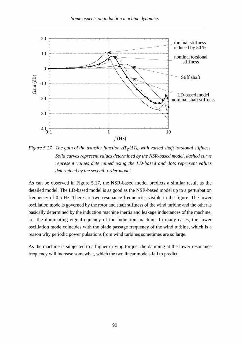
Some aspects on induction machine dynamics
90
-40
-30
-20
-10
0
10
20
0.1 1 10
Gai
n (d
B)
torsinal stiffnessreduced by 50 %
nominal torsionalstiffness
Stiff shaft
LD-based modelnominal shaft stiffness
f (Hz)
Figure 5.17. The gain of the transfer function ∆Te/∆Tw with varied shaft torsional stiffness.
Solid curves represent values determined by the NSR-based model, dashed curve
represent values determined using the LD-based and dots represent values
determined by the seventh-order model.
As can be observed in Figure 5.17, the NSR-based model predicts a similar result as the
detailed model. The LD-based model is as good as the NSR-based model up to a perturbation
frequency of 0.5 Hz. There are two resonance frequencies visible in the figure. The lower
oscillation mode is governed by the rotor and shaft stiffness of the wind turbine and the other is
basically determined by the induction machine inertia and leakage inductances of the machine,
i.e. the dominating eigenfrequency of the induction machine. In many cases, the lower
oscillation mode coincides with the blade passage frequency of the wind turbine, which is a
reason why periodic power pulsations from wind turbines sometimes are so large.
As the machine is subjected to a higher driving torque, the damping at the lower resonance
frequency will increase somewhat, which the two linear models fail to predict.

Some aspects on induction machine dynamics
91
Also the response to frequency perturbations can be analysed using the NSR-model. For
instance, the simplified transfer function from supply frequency perturbation to
electrodynamical torque is
∆Te
∆ωs =
s3 KJt Jm
α + sK (Jm + J t)
s4 Jt Jm
α + s3 Jm JtK
Bα + s2(Jm + Jt(1 +
K
α)) + s
KJt+ KJmB + K
(5.6)
In Figure 5.18 the magnitude of ∆Te/∆ωs for the wind turbine drive train is compared for a
stiff and a soft shaft. The drive train with a soft shaft is modelled using the seventh-order
model, the NSR-based model and the LD-based model. The machine is operating as generator
driven by a shaft torque of one quarter of the rated one.
0
10
20
30
40
50
0.1 1 10
Gai
n (d
B)
f (Hz)
Figure 5.18. The gain of the transfer function ∆Te/∆ωs with a stiff shaft ( ) and a soft
shaft using diffferent models: NSR-based model ( ), LD-based model
( ) and dots seventh-order model.
As in the previous case where the response to a torque perturbation was presented, the
damping at the lower resonance frequency will increase somewhat, as the machine is subjected
to a higher driving torque, which the two linear models fail to predict.

Some aspects on induction machine dynamics
92

Extrapolation to other machine sizes
93
6 EXTRAPOLATION TO OTHER MACHINE SIZES
In Chapter 4 the response of a 15 kW machine was investigated as the machine was
subjected to different types of perturbations. In this chapter the responses of a large
number of machines are analysed in order to obtain some generally applicable results.
Ahmed-Zaid and Taleb (1991) investigated some step responses of eleven machines in
order to give some guidelines for the selection of an induction machine model. The results
were strongly influenced by the fact that some of the machines had very large rated slips,
about 5 %.
The parameters of 31 machines, ranging in size from 2 kW to 4 MW, are presented in
Table 6.1. Mainly four-pole machines are investigated but also several six-pole ones. The
inductances and resistances of the machines are given in per unit values. The parameters
of machines 21-31 were given by Cathey et al. (1973), i.e., the same source as Ahmed-
Zaid and Taleb (1991) used. The parameters of the other machines were obtained from
manufacturers of induction machines.
If small-signal analysis is applied on the induction machine, the transfer function from
shaft torque to electrodynamical torque is found to have three zeros and five poles. The
locations of the three zeros are close to the locations of three of the poles, and the transfer
function from shaft torque to electrodynamical torque can be simplified to the second
order. Providing that the supply frequency is not too low, a useful approximation of the
transfer function from shaft torque disturbance to electrodynamical torque is
∆Te∆Ts
= H(s) = ω0
2
s2 + 2ξω0s + ω02
(6.1)
where ξ is the damping ratio and ω0 the undamped eigenfrequency.
In Figures 6.1 and 6.2 the undamped eigenfrequencies and damping ratios of the
machines, determined by small-signal analysis, are presented. The machines are operating
as motors loaded by a quarter of rated shaft torque. The machines are not connected to a
load, i.e. the total inertia is the machine inertia only. In Figure 6.1 it can be observed that
the undamped eigenfrequency of an induction machine is lowered as the machine size
increases. A 5 kW machine has a resonance frequency of about 25 Hz and a MW size
induction machine has an undamped eigenfrequency of about 5-10 Hz.

Extrapolation to other machine sizes
94
Table 6.1.Parameters of the investigated induction machines (at 20 ˚C).
No. Power
(kW)
U
(V)
Rs
(%)
Rr
(%)
Lm
(pu)
Lsλ(pu)
Lrλ(pu)
fs(Hz)
p Jm
(kgm2)
Rated
slip
1 4 380 1.93 1.76 0.73 0.039 0.039 50 2 0.015 0.043
2 7.5 400 1.41 1.00 0.57 0.039 0.035 50 3 0.082 0.026
3 11 400 1.46 1.01 0.93 0.042 0.047 50 2 0.073 0.024
4 11 400 1.33 1.05 0.61 0.044 0.040 50 3 0.10 0.027
5 15 400 0.99 1.07 0.70 0.053 0.045 50 3 0.22 0.028
6 15 400 1.21 1.1 1.03 0.044 0.051 50 2 0.094 0.027
7 18.5 400 0.95 0.71 0.93 0.042 0.063 50 2 0.16 0.017
8 22 400 0.87 0.71 1.06 0.045 0.070 50 2 0.19 0.017
9 30 400 0.72 0.72 0.98 0.034 0.056 50 3 0.76 0.017
10 45 400 0.63 0.56 1.20 0.049 0.081 50 2 0.41 0.021
11 180 415 0.78 0.72 1.51 0.049 0.051 50 3 4.5 0.017
12 200 380 0.47 0.63 1.75 0.057 0.081 50 2 2.5 0.017
13 200 690 0.41 0.58 1.89 0.052 0.076 50 2 3.0 0.016
14 200 690 0.31 0.37 1.29 0.052 0.061 50 3 6.6 0.010
15 225 400 0.51 0.51 1.30 0.049 0.093 50 3 7.4 0.013
16 400 690 0.3 0.49 1.98 0.046 0.079 50 2 6.6 0.013
17 100 380 0.73 0.65 1.70 0.055 0.096 50 2 1.1 0.019
18 400 380 0.75 0.5 2.11 0.054 0.080 50 2 7.5 0.015
19 630 380 0.6 0.44 2.03 0.051 0.080 50 2 10.8 0.013
20 800 380 0.53 0.44 2.08 0.051 0.083 50 2 13.0 0.013
21 2.23 220 0.95 1.78 0.70 0.020 0.020 60 2 0.045 0.050
22 18.6 460 1.04 2.23 1.12 0.029 0.029 60 2 0.277 0.058
23 37.2 460 0.73 1.89 1.33 0.031 0.031 60 2 0.83 0.053
24 74.5 460 0.52 2.35 1.45 0.031 0.031 60 2 2.22 0.056
25 186 2300 1.14 0.67 1.74 0.050 0.050 60 2 3.5 0.017
26 372 2300 0.88 0.63 2.19 0.049 0.049 60 2 5.6 0.015
27 596 2300 0.70 0.50 2.35 0.047 0.047 60 2 10.7 0.012
28 745 2300 0.75 0.50 4.43 0.049 0.049 60 2 14.9 0.012
29 1117 2300 0.56 0.37 2.42 0.046 0.046 60 2 22.3 0.009
30 1676 2300 0.44 0.33 2.39 0.041 0.041 60 2 31.9 0.008
31 4470 4160 0.27 0.27 3.31 0.045 0.045 60 2 337 0.007

Extrapolation to other machine sizes
95
0
5
10
15
20
25
30
35
1 10 100 103
104
Eig
enfr
eque
ncy
(Hz)
Machine size (kW)
high-slipmachines (21-24)
Figure 6.1. Undamped eigenfrequency of the 31 investigated induction machines.
0
0.2
0.4
0.6
0.8
1
1 10 100 103
104
Dam
ping
rat
io
Machine size (kW)
high-slip machines (21-24)
Figure 6.2. Damping ratio of the 31 investigated induction machines.

Extrapolation to other machine sizes
96
The result of most of the machines form a general trend. The four high-slip machines 21-
24 presented by Cathey et al. (1973) deviate from the trend of the other machines.
From Figure 6.2 it is clear that the four smaller machines described by Cathey et al.
(1973) have an extremely high damping ratio, caused by the high rotor resistance, while
the damping ratio of the other machines varies between 0.1 and 0.3, independent of the
machine size.
The transfer function from shaft torque to electrodynamical torque in which the stator
resistance has been neglected, (2.54), can be used to obtain approximate values of the
undamped eigenfrequency and damping ratio
ω0NSR = LmLs
U
ωs√ p2
JmL'r(6.2)
ξNSR= Rr2
LsLm
ωsU√ Jm
p2L'r(6.3)
respectively. These equations for estimating the eigenfrequency and damping ratio do not
work well when the damping is very high as in the case of machines 21-24. In Figure 6.3
the undamped eigenfrequency obtained using (6.2) is compared with the one obtained
using small-signal analysis. Machines 21-24 have been excluded. The prediction of the
undamped eigenfrequencies differs less than 1 % for the investigated machines. The
prediction of the damping ratio is, however, not as good as the prediction of the
eigenfrequency. The error function
ε = ξNSR – ξss
ξss(6.4)
is used to determine the error in the prediction of the damping ratio. ξss is the damping
ratio obtained using small-signal analysis. In Figure 6.4 the error in the prediction of the
damping ratio is presented as a function of machine size. Again, machines 21-24 have
been excluded.

Extrapolation to other machine sizes
97
0
5
10
15
20
25
0 5 10 15 20 25Eig
enfr
eque
ncy
estim
ated
acc
ordi
ng to
(6.
2) (
Hz)
Eigenfrequency determined from small-signal analysis (Hz)
Figure 6.3. Comparison of undamped eigenfrequencies.
0
10
20
30
40
50
1 10 100 103
104
Err
or (
%)
Machine size (kW)
Figure 6.4. ξ error prediction as a function of machine size.
The error is largest for smaller machines, which have relatively high stator resistances
compared to the leakage inductances while the error is smaller for the larger machines.

Extrapolation to other machine sizes
98
In Chapter 4 it was shown that the rotor speed and electrodynamical torque response of
the 15 kW machine to shaft torque and supply frequency perturbations could be well
predicted using the NSR-model. From Figure 6.4 it can be noted that the NSR-model can
even better predict the same responses of larger machines.
The damping ratio strongly influences the performance of the induction machine. The
investigated 15 kW machine, operating at 288 V and 43.5 Hz and with an inertia of
0.44 kgm2, has a damping ratio of 0.28, which means that the rotor speed response at
the eigenfrequency is twice the steady-state rotor speed response.
Machine 24, a 100 hp machine with high rated slip, has a damping ratio close to 1. In
Figure 6.5 the rotor speed response, calculated using the Park model, NST I-model, LA-
model, and ND-model, is presented for the machine. It can be noted that the rotor speed
response is not higher than the steady-state response for any perturbation frequency.
Further, it can be observed that the values predicted by the NST I and LA-models
coincide very with the values predicted by the Park model.
The opposite is the 200 kW machine, number 14, with a damping ratio of 0.11, where
the rotor speed response at the eigenfrequency is 20 times (26 dB) the rotor speed
response at steady-state. The rotor speed response predicted by the various models of the
200 kW machine is presented in Figure 6.6. Again, the values predicted by the NST I and
LA-models coincide very well with the values predicted by the Park model. From Figures
6.5 and 6.6 it is obvious that the first-order model predicts a less erroneous rotor speed
response to torque perturbations as the damping ratio increases.
The limit frequencies for the first-order model to determine the rotor speed response to
torque perturbations for the investigated machines are presented as a function of the
damping ratio in Figure 6.7. The limit frequency is defined as the frequency at which the
discrepancy between the investigated model and the Park model exceeds a certain level, in
this case 3 dB (41%) and 0.8 dB (10 %).
The four high-slip machines have very high limit frequencies; none of them has an error
higher that 3 dB compared to the Park model for perturbation frequencies up to 100 Hz
and the machines are thus not visible in Figure 6.7. Two of the high-slip machines have a
0.8 dB limit frequency of 70 % while the other two are not visible in Figure 6.7 since
they have an error of less than 0.8 dB for all perturbation frequencies. The limit
frequencies for the other machines are between 10 and 40 % depending on the desired
accuracy and damping ratio.
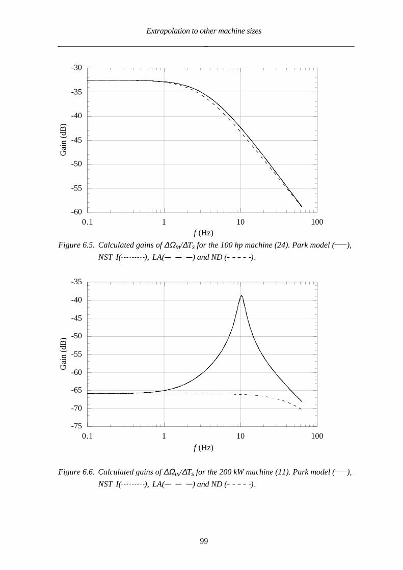
Extrapolation to other machine sizes
99
-60
-55
-50
-45
-40
-35
-30
0.1 1 10 100
Gai
n (d
B)
f (Hz)
Figure 6.5. Calculated gains of ∆Ωm/∆Ts for the 100 hp machine (24). Park model ( ),
NST I( ), LA( ) and ND ( ).
-75
-70
-65
-60
-55
-50
-45
-40
-35
0.1 1 10 100
Gai
n (d
B)
f (Hz)
Figure 6.6. Calculated gains of ∆Ωm/∆Ts for the 200 kW machine (11). Park model ( ),
NST I( ), LA( ) and ND ( ).

Extrapolation to other machine sizes
100
10
100
0.1 1
Lim
it fr
eque
ncy
(%)
Damping ratio
Figure 6.7. Limit frequency for the ND-model to predict the rotor speed response to
torque perturbations. Dots are 3 dB error limits and crosses are 0.8 dB error
limits. The limit frequencies are expressed as percentage of the
eigenfrequencies.
It is important to point out that the damping ratio is of little or no importance for the
possibility of using simpler models to predict the other transfer function characteristics.
The 3 dB limit frequencies of the NST-models, LA-model and ND-model were deter-
mined for the different transfer functions of the 31 machines. The moments of inertia were
twice the values given in Table 6.1, in order to take into account the moments of inertias
of load connected to the machines. This means that the damping ratio is increased by 41 %
and the eigenfrequency is reduced by 41 % according to (6.3) and (6.2), respectively.
The machines are divided into four groups. Group one consists of the ten smaller
machines 1-10, group two consists of machines 11-20, group three of the high-slip
machines 21-24, and group four consists of the seven larger machines 25-31 described
by Cathey et al. (1973). In Tables 6.2-6.9 the 0.8 dB and 3 dB limit frequencies are
presented for the different transfer functions and different models. The machines are
operating as motors loaded by rated torque as the limit frequencies of the LA-model is
determined and as motor loaded by a one quarter of rated torque as the limit frequencies
of the other models are determined. The operating point is in most cases of little
importance for the performance of the reduced-order models, except for the LA-model.
The limit frequencies of the LA-model are generally lowered as the shaft torque increases,
both in motor and generator operation, which is caused by the fact that the damping is

Extrapolation to other machine sizes
101
underestimated. Especially erroneous is the prediction of the damping of machines 11-20
in the cases where they are connected to loads having a very low moment of inertia and
operating with a shaft torque higher than the rated one.
The limit frequencies are independent of the disturbance magnitude at least up to a voltage
magnitude perturbation of 60 % (peak ot peak), a shaft torque perturbation magnitude of
100 % and a supply frequency perturbation magnitude of 10 %. Table 6.2 and 6.3
present the limit frequencies for the ND-model.
Table 6.2. Approximate 0.8 dB limit frequencies for the ND-model.
1-10 11-20 21-24 25-31
Lowest
upper limit
for all
machines∆Ωm∆Ts
1-4 1 5-99 0.7-1.5 1 *
∆Te∆Ts
2.5-5 2 15-25 1-2 1 *
∆P∆Ts
2.5-5 2 15-25 1-2 1 *
∆Q∆Ts
0.5-5 1-2 0.5-30 2-5 0.5
∆Is∆Ts
4-8 2-3 15 1-3 1
∆Ωm
∆ωs2.5-5 2 7-45 1.2 1 *
∆Te
∆ωs2.5-5 2 7-45 1.2 1 *
∆P
∆ωs2.5-5 2 7-40 1-2 1 *
∆Q
∆ωs0.1-0.7 0.1 0.3-1.3 0.02-0.3 0.02
∆Is∆ωs
0.07-5 0.004-0.03 0.3-30 0.002-1.3 0.002
∆Ωm∆U
0.7-1.5 0.6-0.9 2-3 0.7-1 0.5
∆Te∆U
0.7-1.5 0.6-0.9 2-3 0.7-1 0.5
∆P∆U
0.03-0.2 0.002-0.02 0.2-4 0.01-1 0.002
∆Q∆U
0.2-1 0.1-0.2 0.9-1.6 0.05-0.2 0.05
∆Is∆U
0.08-0.5 0.01-0.05 0.2-0.7 0.004-0.1 0.004
* about 30 % of the dominating eigenfrequency for respective machine

Extrapolation to other machine sizes
102
Table 6.3. Approximate 3 dB limit frequencies for the ND-model.
1-10 11-20 21-24 25-31
Lowest
upper limit
for all
machines∆Ωm∆Ts
2-8 2 >100 1.5-3 2 *
∆Te∆Ts
5-10 4 25-40 2-4 2 *
∆P∆Ts
5-10 4 25-40 2-4 2 *
∆Q∆Ts
1-8 8 1-40 4-9 1
∆Is∆Ts
5-21 4 25 2-5 2
∆Ωm
∆ωs4-9 4 40-50 2-4 2 *
∆Te
∆ωs4-9 4 40-50 2-4 2 *
∆P
∆ωs4-9 4 40-50 2-4 2 *
∆Q
∆ωs0.3-1.5 0.2-0.4 0.5-2.3 0.05-4 0.05
∆Is∆ωs
0.1-7.2 0.01-0.1 15-40 2-5 0.01
∆Ωm∆U
1.5-3 1.5 5 1.5-2 1.5
∆Te∆U
1.5-3 1.5 5 1.5-2 1.5
∆P∆U
0.1-0.6 0.04-3 5 1.5-3 0.01
∆Q∆U
0.5-2.5 0.3-0.4 2-4 0.1-0.5 0.1
∆Is∆U
0.1-1.2 0.01-0.1 0.5-1.5 0.01-0.2 0.01
* about 55 % of the dominating eigenfrequency for respective machine
The ∆Ωm, ∆Te and ∆P responses to ∆ωs and ∆Ts perturbations predicted by the ND-
model could accurately be described for all the machines (except the high-slip machines
which have higher limit frequencies) as a percentage of the eigenfrequency. This is not
the case with the other combinations of input and output signals. The ∆Ωm, ∆Te and ∆P
responses to ∆ωs and ∆Ts perturbations could be determined up to a perturbation
frequency of 30 % of the dominating eigenfrequency (i.e. at least up to 2 Hz) before the
discrepancy to the Park model reached 10 %.

Extrapolation to other machine sizes
103
The ∆Ωm, ∆Te responses to ∆U perturbations as well as the ∆Q and ∆Is responses to ∆Ts
perturbations can be predicted up to a perturbation frequency of at least 0.5 Hz. The
prediction of the other transfer function characteristics is otherwise poor.
The responses predicted by using the ND-model vary strongly between the different
induction machine groups. A first-order model of a high-slip machine can better predict
the responses of the induction machine while first-order models of other machines have
poorer performance. Table 6.4 and 6.5 present the limit frequencies for the LA-model.
Table 6.4. Approximate 0.8 dB limit frequencies for the LA-model.
1-10 11-20 21-24 25-31
Lowest
upper limit
for all
machines∆Ωm∆Ts
3-7 2-3 99 2-4 2
∆Te∆Ts
5-10 3-4 25-55 3-5 3
∆P∆Ts
5-10 3-4 25-55 3-5 3
∆Q∆Ts
1-5 1 10-16 1-2 1
∆Is∆Ts
2-7 2 35-50 2-4 2
∆Ωm
∆ωs5-15 3-4 15 4-24 3
∆Te
∆ωs5-15 3-4 15 4-24 3
∆P
∆ωs5-15 3-4 15 4-20 3
∆Q
∆ωs0.003-5 0.05-0.1 0.02-0.3 0.02-0.08 0.003
∆Is∆ωs
0.1-0.4 0.1-0.2 15 0.3-2.6 0.1
∆Ωm∆U
1-3 1 4 1 1
∆Te∆U
1-3 1 4 1 1
∆P∆U
0.1-0.2 0.1 4 0.1-1.5 0.1
∆Q∆U
0.1-1 0.1 0.5-1 0.1 0.1
∆Is∆U
0.3-1 0.6-3 0.3-0.9 1-3 0.3

Extrapolation to other machine sizes
104
Table 6.5. Approximate 3 dB limit frequencies for the LA-model.
1-10 11-20 21-24 25-31
Lowest
upper limit
for all
machines∆Ωm∆Ts
6-99 4-6 >100 >100 4
∆Te∆Ts
6-47 4-6 50-60 50-60 4
∆P∆Ts
6-47 5 50-60 55-60 4
∆Q∆Ts
2-11 2-3 20-50 2-4 2
∆Is∆Ts
6-40 4-5 45-55 50-60 4
∆Ωm
∆ωs6-30 5-6 25 40 5
∆Te
∆ωs6-30 5-6 25 40 5
∆P
∆ωs6-25 5-6 25 30-35 5
∆Q
∆ωs0.02-7.7 0.1-0.3 0.6-10 0.1-0.7 0.02
∆Is∆ωs
0.5-30 4-5 25 35 0.5
∆Ωm∆U
1.5-5 1.5 8 1.5-2.5 1.5
∆Te∆U
1.5-5 1.5 8 1.5-2.5 1.5
∆P∆U
0.3-8 2 8 1.5-3 0.3
∆Q∆U
0.2-2 0.01-0.1 1.5-3 0.01-0.2 0.01
∆Is∆U
0.5-6 4 1-13 3-9 0.5
The LA-model predicts the ∆Te, ∆Ωm and ∆P responses to ∆Ts and ∆ωs perturbations up
to a perturbation frequency of at least 3 Hz before the discrepancy to the Park model
reaches 10 %. The transfer functions ∆Q/∆Ts, ∆Is∆Ts, ∆Ωm/∆U as well as ∆Te/∆U can
be predicted up to a perturbation frequency of 1.5 Hz. The prediction of the other transfer
functions is limited to extremely low-frequency perturbations. The high-slip machines are
more successfully modelled by a second-order model than the other machines.

Extrapolation to other machine sizes
105
In Table 6.6 and 6.7 the limit frequencies for the NST I-model are presented.
Table 6.6. Approximate 0.8 dB limit frequencies for the NST I-model.
1-10 11-20 21-24 25-31
Lowest
upper limit
for all
machines∆Ωm∆Ts
15-99 >100 >100 >100 15
∆Te∆Ts
15-45 50 50 50 15
∆P∆Ts
15-45 50 50 50 15
∆Q∆Ts
10-25 15-20 15-20 15 10
∆Is∆Ts
20-35 40 35-45 35 20
∆Ωm
∆ωs10-15 15 15 18 10
∆Te
∆ωs10-15 15 15 18 10
∆P
∆ωs10-15 15 15 18 10
∆Q
∆ωs10-15 15 10-16 18 10
∆Is∆ωs
5-15 15 15 18 5
∆Ωm∆U
1-2 1 3 1-1.5 1
∆Te∆U
1-2 1 3 1-1.5 1
∆P∆U
0.05-0.4 0.003-0.04 3 0.01-2 0.003
∆Q∆U
10-15 15 15 18 10
∆Is∆U
7-17 5 15 3-15 3

Extrapolation to other machine sizes
106
Table 6.7. Approximate 3 dB limit frequencies for the NST I-model.
1-10 11-20 21-24 25-31
Lowest
upper limit
for all
machines∆Ωm∆Ts
>100 >100 >100 >100 >100
∆Te∆Ts
40-50 50 50-55 55 40
∆P∆Ts
40-50 50 50-55 55 40
∆Q∆Ts
20-25 25 30 25 20
∆Is∆Ts
20-40 45 40-50 50-60 20
∆Ωm
∆ωs25-30 25 30 32 25
∆Te
∆ωs25-30 25 30 32 25
∆P
∆ωs25 25 30 32 25
∆Q
∆ωs25 25 30 32 25
∆Is∆ωs
10-30 25 30 33 10
∆Ωm∆U
2-4 2 4-5 2 2
∆Te∆U
2-4 2 4-5 2 2
∆P∆U
4-7 2-6 5 2-3 2
∆Q∆U
20-30 28 30 33 20
∆Is∆U
25 25 30 25 25
Again, the samme pattern can be observed: The high-slip machines are best suited to be
modelled by the NST I-model. The NST I-model can predict with a 10 % accuracy the
responses to ∆Ts and ∆ωs perturbations up to at least 10 Hz (20 Hz with a 3 dB
accuracy) except for the prediction of ∆Is/∆ωs, which is limited to 5 Hz (10 Hz with a 3
dB accuracy). The 10 % error frequency limit for ∆Ωm/∆U and ∆Te/∆U is about 1 Hz,
for ∆Q/∆U 10 Hz and for ∆Is/∆U 5 Hz. The ∆P response to ∆U perturbations has an
extremely low limit frequency for a 10 % accuracy, for a 3dB accuracy the limit
frequency is about 2 Hz.

Extrapolation to other machine sizes
107
In Table 6.8 and 6.9 the limit frequencies for the NST III-model are presented.
Table 6.8. Approximate 0.8 dB limit frequencies for the NST III-model.
1-10 11-20 21-24 25-31
Lowest
upper limit
for all
machines∆Ωm∆Ts
>100 >100 >100 >100 >100
∆Te∆Ts
30-40 50 45-55 50 30
∆P∆Ts
30-40 50 45-55 50 30
∆Q∆Ts
13-22 15 20 15 15
∆Is∆Ts
15-35 40 30-40 35-50 15
∆Ωm
∆ωs30 28 30 35 30
∆Te
∆ωs15-21 16 20 20 15
∆P
∆ωs0.5-20 16 20 20 15
∆Q
∆ωs2-15 16 1 20 1
∆Is∆ωs
4-20 16 15-30 20 4
∆Ωm∆U
5-15 15 7 15 5
∆Te∆U
0 0 0 0 0
∆P∆U
0.08-2 0.001-0.8 0.002-0.04 0.001-0.3 0.0003
∆Q∆U
15-20 16 25 18 15
∆Is∆U
10-15 6-12 0.7-13 0.5-12 0.5

Extrapolation to other machine sizes
108
Table 6.9. Approximate 3 dB limit frequencies for the NST III-model.
1-10 11-20 21-24 25-31
Lowest
upper limit
for all
machines∆Ωm∆Ts
>100 >100 >100 >100 >100
∆Te∆Ts
40-50 50 50 55 40
∆P∆Ts
40-50 50 50 55 40
∆Q∆Ts
20-30 25 30 25 25
∆Is∆Ts
25-45 45 40-50 50-60 25
∆Ωm
∆ωs40-60 40 45 45 40
∆Te
∆ωs30-35 30 35 35 30
∆P
∆ωs30 25 35 35 25
∆Q
∆ωs30 25 30-35 35 25
∆Is∆ωs
6-30 28 35 35 6
∆Ωm∆U
25 27 7-30 35 25
∆Te∆U
0 0 0-2 0 0
∆P∆U
1-4 0.04-1.5 0.007-0.1 0.003-2 0.0006
∆Q∆U
28-34 28 35 35 30
∆Is∆U
25-30 25 20-35 20-30 20
The NST III-model has generally somewhat higher limit frequencies than the NST I-
model. However, the prediction of ∆Q/∆ωs, ∆Is/∆ωs, ∆Te/∆U, ∆P/∆U, ∆Q/∆U and
∆Is/∆U using the NST III-model is limited to lower frequencies compared to using the
NST I-model.

Extrapolation to other machine sizes
109
For power system analysis, the most interesting quantities are the active and reactive
power responses to voltage and frequency disturbances. It can be observed that first- and
second-order models are not well suited for this task. Further, it can be observed that the
NST III-model is less suited than the NST I-model for this assignment. The NST I-model
can predict the reactive power response up to at least 10 Hz with an error less than 10 %.
The active power response predicted by a third-order model is less accurate. However,
the magnitude of the active power response to frequency and voltage perturbations is low
as long as the disturbances are limited to a few Hz and is thus not as important to model
correctly as the reactive power response. The other responses are of minor importance for
power system analysis.
It is possible to use either a first-order or second-order model to model the induction
machine as a wind turbine generator. This is providing that it is the mechanical system
that is studied, rather than the electrical impact of the wind turbine on the grid. The
dominating eigenfrequency of a 225 kW wind turbine is about 1.5 Hz and a MW-size
wind turbine has a dominating eigenfrequency of about 0.8 Hz. Below 30 % of the
dominating eigenfrequency, a first-order model predicts results with an error less than
10 %. At higher perturbation frequencies, a second-order model is a more suitable
choice.

Extrapolation to other machine sizes
110
Conclusions
111
7. CONCLUSIONS
The Park model very well predicts the rotor speed, electrodynamical torque, active
power, reactive power and stator current responses to perturbations in the shaft torque,
supply frequency and voltage magnitude. The predicted electric power and stator current
responses to very low-frequency perturbations in the voltage magnitude are improved if
the iron losses are taken into account.
The performance of the reduced-order models, i.e. the models of lower order than the
Park model, depends on the type of induction machine investigated. High-slip machines
as well as machines that have a low ratio between the stator resistance and leakage
reactances are best suited to be represented by reduced-order models. Small machines and
machines having a rated voltage that is lower than "the normal rated voltage for a machine
of that size" are more difficult to represent by reduced-order models.
The first-order model, ND-model, of the induction machine can be used to predict the
rotor speed, electrodynamical torque and active power responses to torque and frequency
perturbations up to a perturbation frequency of 30 % of the eigenfrequency if an error of
10 % is acceptable, i.e., 10 % discrepancy between the results predicted by the ND-
model and the Park model. MW-size machines have an eigenfrequency of about 5-10 Hz
and machines with a rating of a few kW have an eigenfrequency of about 25 Hz. The
damping ratio of induction machines varies strongly but is usually not important in
determining the frequency region in which a reduced-order model can be used.
The ND-model can also be used to predict the rotor speed and electrodynamical torque
responses to voltage magnitude perturbations up to a perturbation frequency of 0.5 -
5 Hz depending on the accuracy desired as well as machine investigated. A high ratio
between the stator resistance and leakage reactances leads to a lower value while a high-
slip machine has a higher value.
The LA-model, a non-linear second-order model, predicts the rotor speed,
electrodynamical torque and electric power responses to torque and frequency
perturbations up to a perturbation frequency of at least 3 Hz, if an error of 10 % is
acceptable. The discrepancy between the results obtained using the LA-model and the
Park model depends strongly on the static shaft torque. At no-load, the LA-model can be
used to determine the responses to higher perturbation frequencies. In predicting the
responses to voltage magnitude perturbations, the LA-model is approximately as useful as
a first-order model.

Conclusions
112
The simpler third-order model, the NST I-model, predicts well all the responses to torque
and frequency perturbations up to at least 10 Hz if an error of 10 % is acceptable. In
predicting the rotor speed, electrodynamical torque and electric power responses to
voltage magnitude perturbations, the NST I-model is as useful as a first- or second-order
model. Stator current and reactive power responses can, however, be predicted much
better than by an LA- or ND-model, up to a perturbation frequency of at least 10 Hz for
the reactive power response and at least 3 Hz for the stator current response.
The more advanced third-order model, the NST III-model, generally predicts better
responses than the NST I-model. However, the stator current and reactive power
responses to frequency and voltage perturbations are predicted less accurately and the
electrodynamical torque response to voltage perturbations is inaccurate also for extremely
low-frequency perturbations.
The conclusion drawn here is that for power system analysis it is suitable to use the NST
I-model if the computational effort is a problem, otherwise a Park model is, of course, the
best choice. The advantage of the NST I-model is that the reactive power response to
supply frequency and voltage magnitude perturbations is well predicted up to at least
10 Hz.
Two reduced-order linear models were investigated: a first-order model, the LD-model
and a second-order model, the NSR-model. These models are not suited to determine the
electrical impact of induction machines. Instead, the field of application for these models
is to represent the induction machine in mechanical systems, for instance, in a wind
turbine or a reciprocating compressor drive. An example was demonstrated where the
drive-train of a wind turbine was modelled using the LD-model and the NSR-model to
represent the induction generator. The ND-model is suitable to use if the upper
perturbation frequency is about 0.5 Hz while the NSR-model can handle perturbation
frequencies up to at least 10 Hz. The rotor speed and electrodynamical torque responses
of these models are very similar to those predicted by non-linear models of the same
orders. The difference is that the linear models do not predict a correct steady-state
response.
The responses to supply frequency and torque perturbations depend only slightly on the
static shaft torque if temperature changes are not taken into account. Since the damping of
the machine is mainly governed by the rotor resistance, the damping is improved
substantially as the machine gets warmer; the damping ratio can be increased by 100 %
for the investigated 15 kW machine compared to the case where the machine is cold. The

Conclusions
113
response to voltage magnitude perturbations, on the other hand, depends strongly on the
static shaft torque, even if temperature changes are not taken into account.
In the steady-state operating region, the skin effect in the rotor winding is of minor
importance for the investigated 15 kW machine; the damping was improved by about
10 %. At nominal flux levels or below nominal flux levels, the main flux saturation only
slightly affected the responses of the investigated machine. At a flux level of 120 % of
the nominal one, the very low-frequency rotor speed and electrodynamical torque
responses were influenced by the main flux saturation.
The induction machine characteristics are strongly influenced by the steady-state supply
frequency even if the flux in the machine is kept constant. As the supply frequency is
lowered, the damping ratio is reduced as well. For the 15 kW machine, the damping ratio
was reduced to about one third as the supply frequency was lowered from 43.5 to 15 Hz.

Conclusions
114

References
115
REFERENCES
Adkins, B., Harley, R., 1975. "The general theory of alternating current machines:
application to practical problems", Chapman and Hall, London
Ahmed-Zaid, S., Taleb, M., 1991. "Structural modeling of small and large induction
machines using integral manifolds", IEEE Transactions on Energy Conversion, vol. 6,
no. 3, pp. 529-535
Al-Bahrani, A.H., Mohamadein, A.L., Al-Ohaly, A.A., 1988. "Dynamic response of a
group of induction motors operating in parallel", Electric Machines and Power Systems,
vol.15, pp. 269-281
Cathey, J.J., Cavin, R.K., Ayoub, A.K., 1973. "Transient load model of an induction
motor", IEEE Transactions on Power Apparatus and Systems, vol. 92, no. 4, pp. 1399-
1406
Crow, M.L., 1994. "Dynamics of voltage instability and collapse", International Journal
of Electric Power and Energy Systems, vol. 16, no. 4, pp. 235-241
de Mello, F.P., Hannett, L.N., 1981. "Large scale induction generators for power
systems", IEEE Transactions on Power Apparatus and Systems, vol. 100, no. 5, pp.
2610-2618
Deleroi,W., 1970. "Berücksichtigung der Eisensättigung für dynamische Betriebs-
zustände", Archiv für Elektrotechnik, vol. 54, pp. 31-42
Dell'Aquila, A., Salvatore, L., Savino, M., 1984. "Analysis and development of detailed
inverter-fed induction machine equivalent circuits from standstill frequency response and
on-line harmonic impedance measurements", in Conference Proceedings of the
International Conference on Electrical Machines (ICEM'84), Lausanne, Switzerland, 18-
21 September 1984, pp. 376-379
Derbel, N., Kamoun, M.B.A., Poloujadoff, M., 1995. "On the order reduction of
induction machine during start-up", IEEE Transactions on Energy Conversion, vol. 10,
no. 4, pp. 655-660

References
116
Ertem, S., Baghzouz, Y., 1988. "A fast recursive solution for induction motor
transients", IEEE Transactions on Industry Applications, vol. 24, no. 5, pp. 758-764
Ertem, S., Baghzouz, Y., 1989. "A variable-order model of induction machines",
International Journal of Modelling and Simulation, vol. 9, no. 2, pp. 44-48
Estanqueiro, A.I., Aguiar, R., Saraiva, J.G., Castro, R.M.G., Ferriera de Jesus, J.M.,
1993. "The development and application of a model for power output fluctuations in a
wind park", Proceedings of 1993 European Community Wind Energy Conference
(ECWEC'93), Lübeck-Travemünde, Germany, 8-12 March 1993, pp. 798-801
Freise, W., Jordan, H., Nacke, H., 1964. "Experimentelle Ermittlung der erzwungenen
Pendelungen von Drehstrom-Asynchronmaschinen", ETZ-A vol. 85, no. 12, pp. 370-
372
Hakim, M.M.A., Berg, G.J., 1976. "Dynamic single-unit representation of induction
motor groups", IEEE Transactions on Power Apparatus and Systems, vol. 95, no. 1, pp.
155-161
Hallenius, K.E., 1982. "Contributions to the theory of saturated electrical machines",
Doctoral Thesis, Technical Report no. 122, Chalmers University of Technology,
Göteborg, Sweden
Healey, R.C., Williamson, S., Smith, A.C., 1995. "Improved cage rotor models for
vector controlled induction motors", IEEE Transactions on Industry Applications, vol.
31, no. 4, pp. 812-822
Hinrichsen, E.N., Nolan, P.J., 1982. "Dynamics and stability of wind turbine
generators", IEEE Transactions on Power Apparatus and Systems, vol. 101, no. 8, pp.
2640-2648
Iliceto, F., Capasso, A., 1974. "Dynamic equivalents of asynchronous motor loads in
system stability studies", IEEE Transactions on Power Apparatus and Systems, vol. 93,
no. 5, pp. 1650-1659
Khalil, N.A., Tan, O.T., Baran, I.U., 1982. "Reduced order models for double-cage
induction motors", IEEE Transactions on Power Apparatus and Systems, vol. 101, no.
9, pp. 3135-3140

References
117
Kovacs, P.K., 1984. "Transient phenomena in electrical machines", Elsevier, Budapest
Krause, P.C., Rodriguez, F.D., Wasynchuk, O., Mojica, D.A., 1987. "Neglecting
stator transients when representing isolated operation of induction machines", IEEE
Transactions on Power Systems, vol. 2, no. 1, pp. 183-188
Kron, A.W., Lorenzon, H.W., 1969. "Die selbsterregten Pendelungen von Drehstrom-
Asynchronmaschinen", ETZ-A, vol. 90, no. 9, pp. 200-205
Kylander, G., 1995. "Thermal modelling of small cage induction motors", Doctoral
Thesis, Technical Report no. 265, Chalmers University of Technology, Göteborg,
Sweden
Leonhard, A., 1966. "Die Asynchronmaschine bei periodischen und sprungartigen
Belastungsänderungen", Elektrotechnik und Maschinenbau, vol. 83, no. 6, pp. 357-359
Lorenzen, H.W., 1967. "Der Einfluβ der Stromverdrängung auf die erzwungenen
Pendelungen von Asynchronmaschinen", ETZ-A, vol. 88, no. 18, pp. 445-451
Mayeda, T., Komukai, T., Uemura, Y., Satoh, S., 1985. "Some considerations on
oscillation modes of power systems including induction motors", Electrical Engineering
in Japan, vol. 105, no. 3, pp. 113-122, USA
Melkebeek, J.A.A., 1980. "Stabiliteitsonderzoek van de Spanningsgevoede Induktie-
motor", Doctoral thesis, Gent State University, Gent, Belgium
Melkebeek, J.A.A., 1983. "Magnetising-field saturation and dynamic behaviour of
induction machines. Part 1: Improved calculation method for induction-machine
dynamics", IEE Proceedings B, vol. 130, no. 1, pp. 1-9
Meyer, A., 1976. "Einfluss der Stromverdrängung auf den stationären Betrieb und die
erzwungenen Pendelungen von Asynchronmaschinenen", Brown Boveri Mitteilungen,
vol. 63, no. 8, pp. 500-507
Mohamadein, A.L., 1978. "Generalised chart, load angle, and stability limit in induction
motors", Electric Machines and Electromechanics, vol. 3, no. 1, pp. 65-74

References
118
Mohamadein, A.L., Al-Bahrani , A.H., Al-Ohaly, A., 1986. "Dynamic performance of a
group of induction motors using load-angle approach", in Conference Proceedings of the
International Conference on Electrical Machines (ICEM'86), München, Germany, 8-10
September 1986, pp. 959-962
Nacke, H., 1962. "Schwingungsverhalten des Asynchronmotors", ETZ-A, vol. 83, no.
24, pp. 793-797
Ohtsuki, H., Yokoyama, A., Sekine, Y., 1991. "Reverse action of on-load tap changer
in association with voltage collapse", IEEE Transactions on Power Systems, vol. 6, no.
1, pp. 300-306
Ojo, O.J., Consoli, A., Lipo, T.A., 1990. "An improved model of saturated induction
machines", IEEE Transactions on Industry Applications, vol. 26, no. 2, pp. 212-221
Palit, B.B., 1978. "Eigenwertuntersuchungen an einer Drehstrom-Asynchronmachine bei
selbsterregten Drehschwingungen", Bull. SEV/VSE, vol. 69, no. 8, pp. 371-376
Peterson, B., 1991. "Oscillations in inverter fed induction motor drives", Licentiate
thesis, Lund Institute of Technology, Lund, Sweden
Proakis, J.G., Manolakis, D.G., 1988. "Introduction to digital signal processing",
Macmillan Publishing Company, New York
Rahim, A., Laldin, A.R., 1987. "Aggregation of induction motor loads for transient
stability studies", IEEE Transactions on Energy Conversion, vol. 2, no. 1, pp. 55-61
Richards, G.G., Tan, O.T., 1981. "Simplified models for induction machine transients
under balanced and unbalanced conditions", IEEE Transactions on Industry Applications,
vol. 17, no. 1, pp. 15-21
Richards, G.G., Tan, O.T., 1986. "Decomposed, reduced order model for double-cage
induction machines", IEEE Transactions on Energy Conversion, vol. 1, no. 3, pp. 87-93
Richards, G.G., 1989. "Reduced order models for an induction motor group during bus
transfer", IEEE Transactions on Power Systems, vol. 4, no. 2, pp. 494-498

References
119
Rodriguez, F.D., Wasynczuk, O., 1987. "A refined method of deriving reduced order
models of induction machines", IEEE Transactions on Energy Conversion, vol. 2, no. 1,
pp. 31-37
Sheinman, Y., Rosen, A., 1991. "A dynamic model for performance calculations of grid-
connected horizontal axis wind turbines", Wind Engineering, vol.15, no.4, pp.211-239
Santjer, F., Gerdes, G., 1994. "Netzrückwirkungen, verursacht durch den Betrieb von
Windkraftanlagen am Netz", DEWI Magazin, no.5, pp. 35-41
Sekine, Y., Ohtsuki, H., 1990. "Cascaded voltage collapse", IEEE Transactions on
Power Systems, vol. 5, no. 1, pp. 250-256
Ueda, R., Takata, S., 1981. "Effects of induction machine load on power system", IEEE
Transactions on Power Apparatus and Systems, vol. 100, no. 5, pp. 2555-2562
Wasynczuk, O., Diao, Y-M., Krause, P.C., 1985. "Theory and comparison of reduced
order models of induction machines", IEEE Transactions on Power Apparatus and
Systems, vol. 104, no. 3, pp. 598-606
Wilkie, J., Leithead, W.E., Anderson, C., 1990. "Modelling of wind turbines by simple
models", Wind Engineering, vol. 14, no. 4, pp. 247-274

References
120

Appendix A: Determination of the induction machine parameters
121
APPENDIX A. DETERMINATION OF THE INDUCTIONMACHINE PARAMETERS
In this Appendix the parameters of the investigated 15 kW machine are determined. The
parameters given by the manufacturer of the 15 kW induction machine investigated are
presented together with the measured values in Table A.1. The equivalent circuit of the
induction machine with the iron loss equivalent is presented in Figure A.1.
Table A.1. Measured values and values given by the manufacturer of the investigated
15 kW machine. (Resistances referred to 20 °C)
Parameter Value given by the
manufacturer
Measured/used values
Rs stator resistance 0.18 Ω 0.184 ΩRr rotor resistance 0.19 Ω 0.175 ΩLm magnetizing inductance 42.6 mH 27 - 43 mH
Lsλ stator leakage
inductance
2.55 mH 2.55 mH
Lrλ rotor leakage
inductance
2.07 mH 2.00 mH
J moment of inertia 0.205 kgm2 (* )
0.45 kgm2 (** )
0.45 kgm2
Rm iron loss equivalent
resistance
166 Ω (50 Hz) 135 Ω (43.5 Hz)
97-48 Ω (30 Hz)
U voltage 380 V 288 V
f frequency 50 Hz 43.5 Hz
(*) induction machine inertia only.
(**) inertia of induction machine, dc-machine (0.22 kgm2) and the two torque transducer couplings (2
times 0.0125 kgm2).

Appendix A: Determination of the induction machine parameters
122
Rs
Rm ωs – pΩm
ωsRr
jωsLsλ
jωsLm
jωsLrλ
Figure A.1. The equivalent circuit with an iron loss equivalent resistance added in
parallel with the magnetizing inductance.
Determining resistance and leakage inductance of the stator
Since no suitable method of separating the stator and rotor leakage inductances was
available, the stator leakage inductance is assumed to be 2.55 mH, which is the value
provided by the manufacturer. Anyway, the separation of the leakage inductances to the
rotor and stator is of little importance for the dynamic performance of the machine, as
long as the total leakage inductance is correct (Grantham 1985, Akbaba et al. 1995). The
stator resistance was measured to be 0.184 Ω at 20 °C.
Determination of magnetizing inductance
The magnetizing inductance, Lm, was determined in the conventional way by means of a
no load test performed at different voltage levels. The magnetizing inductance was also
determined as a function of the temperature for a given flux level. In Figures A.2 and A.3
the measured magnetizing inductance is presented as a function of the magnetizing
current, im, and rotor temperature together with linear function approximations. The
machine is operating at no load.

Appendix A: Determination of the induction machine parameters
123
25
30
35
40
45
10 15 20 25 30
Lm
(m
H)
im (A)
Figure A.2. Measured magnetizing inductance as a function of the magnetizing current.
Rotor temperature 40 °C.
40.5
41
41.5
42
42.5
43
43.5
30 40 50 60 70 80rotor temperature (°C)
Lm
(m
H)
Figure A.3. Measured magnetizing inductance as a function of the rotor temperature.
U = 288 V, f = 43.5 Hz.
The magnetizing inductance may be represented as a linear function of the magnetizing
current and rotor temperature T:
Lm = k1 – k2im + k3T (A.1)
where
k1 = 14.64 H (A.2)

Appendix A: Determination of the induction machine parameters
124
k2 = 0.921 H/A (A.3)
k3=0.04471H/°C (A.4)
for 12 A < Im < 29 A and 30 °C < T < 80 °C
Determination of iron loss equivalent resistance
The iron loss equivalent resistance Rm was determined in the conventional way from a no
load test performed at various voltages and at some different frequencies. At 43.5 Hz,
Rm was found to be 135 Ω and at 50 Hz Rm was found to be 160 Ω, which is very close
to the value given by the manufacturer, 166 Ω. At 30 Hz Rm was found to be 97 Ω.
Determination of rotor leakage inductance
The rotor leakage inductance was determined from a locked-rotor test performed at a
supply frequency of 10 Hz in order to avoid the influence of the skin effect in the rotor
winding. The stator current used was varied between 10 and 40 A in order to determine
at which current level saturation of the leakage inductances becomes important. The rated
rotor current (referred to the stator winding) is 22 A. Up to a rotor current of 30 A the
leakage inductance was constant and at a rotor current of 38 A, the leakage inductance
had been lowered by 2 %. In order to determine the rotor leakage inductance, the
equivalent circuit presented in Figure A.1 was used. Apart from the rotor leakage
inductance, the rotor resistance had not yet been determined. However, the rotor
resistance value affected the determination of the rotor leakage inductance only slightly,
so the rotor resistance was assumed to be 0.19 Ω according to the manufacturer data. The
rotor leakage inductance was found to be 2.03 mH, somewhat less than the value given
by the manufacturer.
Determination of rotor resistance
The rotor resistance, Rr, was not determined from the locked rotor test since the accuracy
of the rotor resistance value may be better by determining the rotor resistance from a load
test. The shaft torque was varied from about rated torque at motor operation to about
rated torque at generator operation at a voltage of 288 V and at a supply frequency of
43.5 Hz. The measured power-slip, torque-slip and reactive power-slip curves are
presented together with curves calculated using two different rotor resistances in Figures
A.4-A.6

Appendix A: Determination of the induction machine parameters
125
-200
-100
0
100
200
-0.04 -0.02 0 0.02 0.04slip (%)
T e (
Nm
)
Figure A.4. Measured and calculated torque-slip curves. Dots represent measured values
and lines show calculated ones. Solid line with Rr = 0.19 Ω and dashed line
with Rr = 0.175 Ω (at 20 °C).
-20
-10
0
10
20
-0.04 -0.02 0 0.02 0.04slip (%)
Pe
(kW
)
Figure A.5. Measured and calculated electric power-slip curves. Dots represent
measured values and lines show calculated ones. Solid line with Rr = 0.19
Ω and dashed line with Rr = 0.175 Ω (at 20 °C).

Appendix A: Determination of the induction machine parameters
126
6
7
8
9
10
-0.04 -0.02 0 0.02 0.04slip (%)
Q (
kVA
r)
Figure A.6. Measured and calculated reactive power-slip curves. Dots represent
measured values and lines show calculated ones. Solid line with Rr = 0.19
Ω and dashed line with Rr = 0.175 Ω (at 20 °C).
As can be noted from Figures A.4-A.6, a rotor resistance of 0.175 Ω predicts the static
behaviour of the induction machine better than the value of 0.19 Ω given by the
manufacturer.
Locked rotor test at variable frequency
The purpose of the variable-frequency locked-rotor test is to determine the rotor cage
characteristics. From the measured characteristics a multiple-cage rotor configuration can
be adapted.
The locked rotor test was performed at different voltage levels and at different supply
frequencies. Throughout the locked rotor measurements, the machine temperature was
kept constant. In order to obtain a voltage with a low harmonic content, a synchronous
generator was used for feeding the machine. The voltages, currents, frequency and
power factor were measured by means of a digital power meter and the torque was
measured by a torque transducer. The locked-rotor torque was determined as the average
torque over one cogging period. The current levels were kept below the rated current in
order not to saturate the machine.
Knowing the magnetizing inductance, the stator leakage inductance and the stator
resistance, the resistance and leakage inductance of the rotor were determined using the
equivalent circuit presented in Figure A.1. Compared to usual locked rotor tests, the

Appendix A: Determination of the induction machine parameters
127
difference here is that the locked rotor torque is measured. This makes a more accurate
determination of the rotor resistance possible.
The rotor resistance is usually determined from the locked-rotor resistance
Rk ≈ Rs + (Lm
Lm + Lrλ)2
Rr + Rcl (A.5)
where Rcl is an equivalent resistance representing the core losses and additional losses.
Rcl is usually not taken into account, which means that the rotor resistance value
becomes somewhat too high. With the knowledge of the locked-rotor torque, it is
possible to separate Rcl from Rr.
The rotor leakage inductance and rotor resistance measured by the locked rotor test are
presented in Figure A.7 and Figure A.8, respectively. The measured rotor winding
characteristics were then used to determine the parameters of the double-cage rotor
winding.
1.5
1.6
1.7
1.8
1.9
2
2.1
0 20 40 60 80 100
Lrλ
(m
H)
f (Hz)
Figure A.7. Measured rotor leakage inductance.

Appendix A: Determination of the induction machine parameters
128
0.15
0.2
0.25
0.3
0.35
0.4
0.45
0.5
0.55
0 20 40 60 80 100
Rr (
Ω)
f (Hz)
Figure A.8. Measured rotor resistance.
References
Akbaba, M., Taleb, M., Rumeli, A., 1995. "Improved estimation of induction machine
parameters", Electric Power Systems Research, 34, p. 65-73
Grantham, C., 1985, "Determination of induction motor parameter variations from a
variable frequency standstill test". Electric Machines and power systems, 10:239-248

Appendix B: Procedure to derive the NST I-model
129
APPENDIX B. PROCEDURE TO DERIVE THE NST I MODEL
The procedure to derive the NST-models have been presented by, for example,
Rodriguez and Wasynczuk (1987). In this Appendix only the NST I-model will be
derived.
The cage induction machine equations can be expressed as
pΨqds = W0Ψqds + Y0Ψqdr + Bs0uqds (B.1)
pΨqdr = Q0Ψqds + Sl0Ψqdr + ΩmSnl0Ψqdr (B.2)
p Ωm = 1Jm
[ΨqdstTsr Ψqdr – Tl] (B.3)
where
p = ddt (B.4)
Ψqds = [Ψqs Ψds]t (B.5)
Ψqdr = [Ψqr Ψdr]t (B.6)
uqds = [uqs uds]t (B.7)
and
W0 =
–R sL s' –ω s
ωs–RsL s'
, Q0 =
ksR rL r'
0
0ksRrL r'
,
Y0 =
krR sL s' 0
0krRsL s'
, Sl0 =
–R rL r'
– ω s
ω s –RrL r'
,
Snl0 = [ ] 0 p – p 0 , Bs0 = [ ]
1 0 0 1 , Tsr =
0
pk rL s'
–pkrL s' 0

Appendix B: Procedure to derive the NST I-model
130
The output signals are determined by
Y = NΨqds + MΨqdr (B.8)
The output signals of Y may be the currents, flux linkages, rotor speed, electrodynamical
torque as well as active and reactive powers. If Y = [ iqs ids]t then
N =
LrLrLs – LmLm
0
0 Lr
LrLs – LmLm
and M =
–LmLrLs – LmLm
0
0 –Lm
LrLs – LmLm
By neglecting the effect of stator transients, i.e, the term pΨqds, the solution of (B.1) is
Ψqds* = – W0-1Y0Ψqdr – W0-1Bs0uqds (B.9)
This term differs from the actual flux linkage Ψqds and, in essence, represents its slow
component. Equations (B.2)-(B.3) with pΨqds neglected, after some algebraic
manipulation, may be expressed as
pΨqdr = [Sl0 – Q0W0-1Y0]Ψqdr + ΩmSnl0Ψqdr - Q0W0-1Bs0uqds (B.10)
pΩm = 1Jm
Ψqdrt[-W0-1Y0]tTsrΨqdr + uqdst[-W0-1Bs0]tTsrΨqdr – Tl (B.11)
Equations (B.10)-(B.11) represent the standard reduced order model of the induction
machine, the NST I-model. An expression for the output signals in terms of the state
variables in (B.10)-(B.11) can be derived by substituting Ψqds*, defined by (B.9) in
(B.8) and rearranging. This gives
Y = [M - NW0-1Y0] Ψqdr – NW0-1Bs0uqds (B.12)
References
Rodriguez, F.D., Wasynczuk, O., 1987. "A refined method of deriving reduced order
models of induction machines", IEEE Transactions on Energy Conversion, vol. 2, no. 1,
pp. 31-37