EUROPEAN ORGANIZATION FOR NUCLEAR RESEARCH (CERN)

CERN-LHCb-DP-2013-002February 13, 2015

Measurement of the trackreconstruction efficiency at LHCb

The LHCb collaboration†

Abstract

The determination of track reconstruction efficiencies at LHCb using J/ψ → µ+µ−

decays is presented. Efficiencies above 95% are found for the data taking periods in2010, 2011, and 2012. The ratio of the track reconstruction efficiency of muons indata and simulation is compatible with unity and measured with an uncertainty of0.8 % for data taking in 2010, and at a precision of 0.4 % for data taking in 2011and 2012. For hadrons an additional 1.4 % uncertainty due to material interactionsis assumed. This result is crucial for accurate cross section and branching fractionmeasurements in LHCb.

Published in JINST 10 (2015) P02007

c© CERN on behalf of the LHCb collaboration, license CC-BY-3.0.

†Authors are listed on the following pages.

arX

iv:1

408.

1251

v2 [

hep-

ex]

13

Feb

2015

ii

LHCb collaboration

R. Aaij41, B. Adeva37, M. Adinolfi46, A. Affolder52, Z. Ajaltouni5, S. Akar6, J. Albrecht9,F. Alessio38, M. Alexander51, S. Ali41, G. Alkhazov30, P. Alvarez Cartelle37, A.A. Alves Jr25,38,S. Amato2, S. Amerio22, Y. Amhis7, L. An3, L. Anderlini17,g, J. Anderson40, R. Andreassen57,M. Andreotti16,f , J.E. Andrews58, R.B. Appleby54, O. Aquines Gutierrez10, F. Archilli38,A. Artamonov35, M. Artuso59, E. Aslanides6, G. Auriemma25,n, M. Baalouch5, S. Bachmann11,J.J. Back48, A. Badalov36, W. Baldini16, R.J. Barlow54, C. Barschel38, S. Barsuk7, W. Barter47,V. Batozskaya28, V. Battista39, A. Bay39, L. Beaucourt4, J. Beddow51, F. Bedeschi23,I. Bediaga1, S. Belogurov31, K. Belous35, I. Belyaev31, E. Ben-Haim8, G. Bencivenni18,S. Benson38, J. Benton46, A. Berezhnoy32, R. Bernet40, M.-O. Bettler47, M. van Beuzekom41,A. Bien11, S. Bifani45, T. Bird54, A. Bizzeti17,i, P.M. Bjørnstad54, T. Blake48, F. Blanc39,J. Blouw10, S. Blusk59, V. Bocci25, A. Bondar34, N. Bondar30,38, W. Bonivento15,38, S. Borghi54,A. Borgia59, M. Borsato7, T.J.V. Bowcock52, E. Bowen40, C. Bozzi16, T. Brambach9,J. van den Brand42, J. Bressieux39, D. Brett54, M. Britsch10, T. Britton59, J. Brodzicka54,N.H. Brook46, H. Brown52, A. Bursche40, G. Busetto22,r, J. Buytaert38, S. Cadeddu15,R. Calabrese16,f , M. Calvi20,k, M. Calvo Gomez36,p, P. Campana18,38, D. Campora Perez38,A. Carbone14,d, G. Carboni24,l, R. Cardinale19,38,j , A. Cardini15, L. Carson50,K. Carvalho Akiba2, G. Casse52, L. Cassina20, L. Castillo Garcia38, M. Cattaneo38, Ch. Cauet9,R. Cenci58, M. Charles8, Ph. Charpentier38, S. Chen54, S.-F. Cheung55, N. Chiapolini40,M. Chrzaszcz40,26, K. Ciba38, X. Cid Vidal38, G. Ciezarek53, P.E.L. Clarke50, M. Clemencic38,H.V. Cliff47, J. Closier38, V. Coco38, J. Cogan6, E. Cogneras5, P. Collins38,A. Comerma-Montells11, A. Contu15, A. Cook46, M. Coombes46, S. Coquereau8, G. Corti38,M. Corvo16,f , I. Counts56, B. Couturier38, G.A. Cowan50, D.C. Craik48, M. Cruz Torres60,S. Cunliffe53, R. Currie50, C. D’Ambrosio38, J. Dalseno46, P. David8, P.N.Y. David41, A. Davis57,K. De Bruyn41, S. De Capua54, M. De Cian11, J.M. De Miranda1, L. De Paula2, W. De Silva57,P. De Simone18, D. Decamp4, M. Deckenhoff9, L. Del Buono8, N. Deleage4, D. Derkach55,O. Deschamps5, F. Dettori38, A. Di Canto38, H. Dijkstra38, S. Donleavy52, F. Dordei11,M. Dorigo39, A. Dosil Suarez37, D. Dossett48, A. Dovbnya43, K. Dreimanis52, G. Dujany54,F. Dupertuis39, P. Durante38, R. Dzhelyadin35, A. Dziurda26, A. Dzyuba30, S. Easo49,38,U. Egede53, V. Egorychev31, S. Eidelman34, S. Eisenhardt50, U. Eitschberger9, R. Ekelhof9,L. Eklund51, I. El Rifai5, Ch. Elsasser40, S. Ely59, S. Esen11, H.-M. Evans47, T. Evans55,A. Falabella14, C. Farber11, C. Farinelli41, N. Farley45, S. Farry52, RF Fay52, D. Ferguson50,V. Fernandez Albor37, F. Ferreira Rodrigues1, M. Ferro-Luzzi38, S. Filippov33, M. Fiore16,f ,M. Fiorini16,f , M. Firlej27, C. Fitzpatrick39, T. Fiutowski27, M. Fontana10, F. Fontanelli19,j ,R. Forty38, O. Francisco2, M. Frank38, C. Frei38, M. Frosini17,38,g, J. Fu21,38, E. Furfaro24,l,A. Gallas Torreira37, D. Galli14,d, S. Gallorini22, S. Gambetta19,j , M. Gandelman2, P. Gandini59,Y. Gao3, J. Garcıa Pardinas37, J. Garofoli59, J. Garra Tico47, L. Garrido36, C. Gaspar38,R. Gauld55, L. Gavardi9, G. Gavrilov30, E. Gersabeck11, M. Gersabeck54, T. Gershon48,Ph. Ghez4, A. Gianelle22, S. Giani’39, V. Gibson47, L. Giubega29, V.V. Gligorov38, C. Gobel60,D. Golubkov31, A. Golutvin53,31,38, A. Gomes1,a, C. Gotti20, M. Grabalosa Gandara5,R. Graciani Diaz36, L.A. Granado Cardoso38, E. Grauges36, G. Graziani17, A. Grecu29,E. Greening55, S. Gregson47, P. Griffith45, L. Grillo11, O. Grunberg62, B. Gui59, E. Gushchin33,Yu. Guz35,38, T. Gys38, C. Hadjivasiliou59, G. Haefeli39, C. Haen38, S.C. Haines47, S. Hall53,B. Hamilton58, T. Hampson46, X. Han11, S. Hansmann-Menzemer11, N. Harnew55,S.T. Harnew46, J. Harrison54, J. He38, T. Head38, V. Heijne41, K. Hennessy52, P. Henrard5,

iii

L. Henry8, J.A. Hernando Morata37, E. van Herwijnen38, M. Heß62, A. Hicheur1, D. Hill55,M. Hoballah5, C. Hombach54, W. Hulsbergen41, P. Hunt55, N. Hussain55, D. Hutchcroft52,D. Hynds51, M. Idzik27, P. Ilten56, R. Jacobsson38, A. Jaeger11, J. Jalocha55, E. Jans41,P. Jaton39, A. Jawahery58, F. Jing3, M. John55, D. Johnson55, C.R. Jones47, C. Joram38,B. Jost38, N. Jurik59, M. Kaballo9, S. Kandybei43, W. Kanso6, M. Karacson38, T.M. Karbach38,S. Karodia51, M. Kelsey59, I.R. Kenyon45, T. Ketel42, B. Khanji20, C. Khurewathanakul39,S. Klaver54, K. Klimaszewski28, O. Kochebina7, M. Kolpin11, I. Komarov39, R.F. Koopman42,P. Koppenburg41,38, M. Korolev32, A. Kozlinskiy41, L. Kravchuk33, K. Kreplin11, M. Kreps48,G. Krocker11, P. Krokovny34, F. Kruse9, W. Kucewicz26,o, M. Kucharczyk20,26,38,k,V. Kudryavtsev34, K. Kurek28, T. Kvaratskheliya31, V.N. La Thi39, D. Lacarrere38,G. Lafferty54, A. Lai15, D. Lambert50, R.W. Lambert42, G. Lanfranchi18, C. Langenbruch48,B. Langhans38, T. Latham48, C. Lazzeroni45, R. Le Gac6, J. van Leerdam41, J.-P. Lees4,R. Lefevre5, A. Leflat32, J. Lefrancois7, S. Leo23, O. Leroy6, T. Lesiak26, B. Leverington11,Y. Li3, T. Likhomanenko63, M. Liles52, R. Lindner38, C. Linn38, F. Lionetto40, B. Liu15,S. Lohn38, I. Longstaff51, J.H. Lopes2, N. Lopez-March39, P. Lowdon40, H. Lu3, D. Lucchesi22,r,H. Luo50, A. Lupato22, E. Luppi16,f , O. Lupton55, F. Machefert7, I.V. Machikhiliyan31,F. Maciuc29, O. Maev30, S. Malde55, G. Manca15,e, G. Mancinelli6, J. Maratas5, J.F. Marchand4,U. Marconi14, C. Marin Benito36, P. Marino23,t, R. Marki39, J. Marks11, G. Martellotti25,A. Martens8, A. Martın Sanchez7, M. Martinelli41, D. Martinez Santos42, F. Martinez Vidal64,D. Martins Tostes2, A. Massafferri1, R. Matev38, Z. Mathe38, C. Matteuzzi20, A. Mazurov16,f ,M. McCann53, J. McCarthy45, A. McNab54, R. McNulty12, B. McSkelly52, B. Meadows57,F. Meier9, M. Meissner11, M. Merk41, D.A. Milanes8, M.-N. Minard4, N. Moggi14,J. Molina Rodriguez60, S. Monteil5, M. Morandin22, P. Morawski27, A. Morda6, M.J. Morello23,t,J. Moron27, A.-B. Morris50, R. Mountain59, F. Muheim50, K. Muller40, M. Mussini14,B. Muster39, P. Naik46, T. Nakada39, R. Nandakumar49, I. Nasteva2, M. Needham50, N. Neri21,S. Neubert38, N. Neufeld38, M. Neuner11, A.D. Nguyen39, T.D. Nguyen39, C. Nguyen-Mau39,q,M. Nicol7, V. Niess5, R. Niet9, N. Nikitin32, T. Nikodem11, A. Novoselov35, D.P. O’Hanlon48,A. Oblakowska-Mucha27, V. Obraztsov35, S. Oggero41, S. Ogilvy51, O. Okhrimenko44,R. Oldeman15,e, G. Onderwater65, M. Orlandea29, J.M. Otalora Goicochea2, P. Owen53,A. Oyanguren64, B.K. Pal59, A. Palano13,c, F. Palombo21,u, M. Palutan18, J. Panman38,A. Papanestis49,38, M. Pappagallo51, L.L. Pappalardo16,f , C. Parkes54, C.J. Parkinson9,45,G. Passaleva17, G.D. Patel52, M. Patel53, C. Patrignani19,j , A. Pazos Alvarez37, A. Pearce54,A. Pellegrino41, M. Pepe Altarelli38, S. Perazzini14,d, E. Perez Trigo37, P. Perret5,M. Perrin-Terrin6, L. Pescatore45, E. Pesen66, K. Petridis53, A. Petrolini19,j ,E. Picatoste Olloqui36, B. Pietrzyk4, T. Pilar48, D. Pinci25, A. Pistone19, S. Playfer50,M. Plo Casasus37, F. Polci8, A. Poluektov48,34, E. Polycarpo2, A. Popov35, D. Popov10,B. Popovici29, C. Potterat2, E. Price46, J. Prisciandaro39, A. Pritchard52, C. Prouve46,V. Pugatch44, A. Puig Navarro39, G. Punzi23,s, W. Qian4, B. Rachwal26, J.H. Rademacker46,B. Rakotomiaramanana39, M. Rama18, M.S. Rangel2, I. Raniuk43, N. Rauschmayr38,G. Raven42, S. Reichert54, M.M. Reid48, A.C. dos Reis1, S. Ricciardi49, S. Richards46, M. Rihl38,K. Rinnert52, V. Rives Molina36, D.A. Roa Romero5, P. Robbe7, A.B. Rodrigues1,E. Rodrigues54, P. Rodriguez Perez54, S. Roiser38, V. Romanovsky35, A. Romero Vidal37,M. Rotondo22, J. Rouvinet39, T. Ruf38, F. Ruffini23, H. Ruiz36, P. Ruiz Valls64,J.J. Saborido Silva37, N. Sagidova30, P. Sail51, B. Saitta15,e, V. Salustino Guimaraes2,C. Sanchez Mayordomo64, B. Sanmartin Sedes37, R. Santacesaria25, C. Santamarina Rios37,E. Santovetti24,l, A. Sarti18,m, C. Satriano25,n, A. Satta24, D.M. Saunders46, M. Savrie16,f ,

iv

D. Savrina31,32, M. Schiller42, H. Schindler38, M. Schlupp9, M. Schmelling10, B. Schmidt38,O. Schneider39, A. Schopper38, M.-H. Schune7, R. Schwemmer38, B. Sciascia18, A. Sciubba25,M. Seco37, A. Semennikov31, I. Sepp53, N. Serra40, J. Serrano6, L. Sestini22, P. Seyfert11,M. Shapkin35, I. Shapoval16,43,f , Y. Shcheglov30, T. Shears52, L. Shekhtman34, V. Shevchenko63,A. Shires9, R. Silva Coutinho48, G. Simi22, M. Sirendi47, N. Skidmore46, T. Skwarnicki59,N.A. Smith52, E. Smith55,49, E. Smith53, J. Smith47, M. Smith54, H. Snoek41, M.D. Sokoloff57,F.J.P. Soler51, F. Soomro39, D. Souza46, B. Souza De Paula2, B. Spaan9, A. Sparkes50,P. Spradlin51, S. Sridharan38, F. Stagni38, M. Stahl11, S. Stahl11, O. Steinkamp40,O. Stenyakin35, S. Stevenson55, S. Stoica29, S. Stone59, B. Storaci40, S. Stracka23,38,M. Straticiuc29, U. Straumann40, R. Stroili22, V.K. Subbiah38, L. Sun57, W. Sutcliffe53,K. Swientek27, S. Swientek9, V. Syropoulos42, M. Szczekowski28, P. Szczypka39,38, D. Szilard2,T. Szumlak27, S. T’Jampens4, M. Teklishyn7, G. Tellarini16,f , F. Teubert38, C. Thomas55,E. Thomas38, J. van Tilburg41, V. Tisserand4, M. Tobin39, S. Tolk42, L. Tomassetti16,f ,D. Tonelli38, S. Topp-Joergensen55, N. Torr55, E. Tournefier4, S. Tourneur39, M.T. Tran39,M. Tresch40, A. Tsaregorodtsev6, P. Tsopelas41, N. Tuning41, M. Ubeda Garcia38, A. Ukleja28,A. Ustyuzhanin63, U. Uwer11, V. Vagnoni14, G. Valenti14, A. Vallier7, R. Vazquez Gomez18,P. Vazquez Regueiro37, C. Vazquez Sierra37, S. Vecchi16, J.J. Velthuis46, M. Veltri17,h,G. Veneziano39, M. Vesterinen11, B. Viaud7, D. Vieira2, M. Vieites Diaz37,X. Vilasis-Cardona36,p, A. Vollhardt40, D. Volyanskyy10, D. Voong46, A. Vorobyev30,V. Vorobyev34, C. Voß62, H. Voss10, J.A. de Vries41, R. Waldi62, C. Wallace48, R. Wallace12,J. Walsh23, S. Wandernoth11, J. Wang59, D.R. Ward47, N.K. Watson45, D. Websdale53,M. Whitehead48, J. Wicht38, D. Wiedner11, G. Wilkinson55, M.P. Williams45, M. Williams56,F.F. Wilson49, J. Wimberley58, J. Wishahi9, W. Wislicki28, M. Witek26, G. Wormser7,S.A. Wotton47, S. Wright47, S. Wu3, K. Wyllie38, Y. Xie61, Z. Xing59, Z. Xu39, Z. Yang3,X. Yuan3, O. Yushchenko35, M. Zangoli14, M. Zavertyaev10,b, L. Zhang59, W.C. Zhang12,Y. Zhang3, A. Zhelezov11, A. Zhokhov31, L. Zhong3, A. Zvyagin38.

1Centro Brasileiro de Pesquisas Fısicas (CBPF), Rio de Janeiro, Brazil2Universidade Federal do Rio de Janeiro (UFRJ), Rio de Janeiro, Brazil3Center for High Energy Physics, Tsinghua University, Beijing, China4LAPP, Universite de Savoie, CNRS/IN2P3, Annecy-Le-Vieux, France5Clermont Universite, Universite Blaise Pascal, CNRS/IN2P3, LPC, Clermont-Ferrand, France6CPPM, Aix-Marseille Universite, CNRS/IN2P3, Marseille, France7LAL, Universite Paris-Sud, CNRS/IN2P3, Orsay, France8LPNHE, Universite Pierre et Marie Curie, Universite Paris Diderot, CNRS/IN2P3, Paris, France9Fakultat Physik, Technische Universitat Dortmund, Dortmund, Germany10Max-Planck-Institut fur Kernphysik (MPIK), Heidelberg, Germany11Physikalisches Institut, Ruprecht-Karls-Universitat Heidelberg, Heidelberg, Germany12School of Physics, University College Dublin, Dublin, Ireland13Sezione INFN di Bari, Bari, Italy14Sezione INFN di Bologna, Bologna, Italy15Sezione INFN di Cagliari, Cagliari, Italy16Sezione INFN di Ferrara, Ferrara, Italy17Sezione INFN di Firenze, Firenze, Italy18Laboratori Nazionali dell’INFN di Frascati, Frascati, Italy19Sezione INFN di Genova, Genova, Italy20Sezione INFN di Milano Bicocca, Milano, Italy21Sezione INFN di Milano, Milano, Italy22Sezione INFN di Padova, Padova, Italy

v

23Sezione INFN di Pisa, Pisa, Italy24Sezione INFN di Roma Tor Vergata, Roma, Italy25Sezione INFN di Roma La Sapienza, Roma, Italy26Henryk Niewodniczanski Institute of Nuclear Physics Polish Academy of Sciences, Krakow, Poland27AGH - University of Science and Technology, Faculty of Physics and Applied Computer Science,Krakow, Poland28National Center for Nuclear Research (NCBJ), Warsaw, Poland29Horia Hulubei National Institute of Physics and Nuclear Engineering, Bucharest-Magurele, Romania30Petersburg Nuclear Physics Institute (PNPI), Gatchina, Russia31Institute of Theoretical and Experimental Physics (ITEP), Moscow, Russia32Institute of Nuclear Physics, Moscow State University (SINP MSU), Moscow, Russia33Institute for Nuclear Research of the Russian Academy of Sciences (INR RAN), Moscow, Russia34Budker Institute of Nuclear Physics (SB RAS) and Novosibirsk State University, Novosibirsk, Russia35Institute for High Energy Physics (IHEP), Protvino, Russia36Universitat de Barcelona, Barcelona, Spain37Universidad de Santiago de Compostela, Santiago de Compostela, Spain38European Organization for Nuclear Research (CERN), Geneva, Switzerland39Ecole Polytechnique Federale de Lausanne (EPFL), Lausanne, Switzerland40Physik-Institut, Universitat Zurich, Zurich, Switzerland41Nikhef National Institute for Subatomic Physics, Amsterdam, The Netherlands42Nikhef National Institute for Subatomic Physics and VU University Amsterdam, Amsterdam, TheNetherlands43NSC Kharkiv Institute of Physics and Technology (NSC KIPT), Kharkiv, Ukraine44Institute for Nuclear Research of the National Academy of Sciences (KINR), Kyiv, Ukraine45University of Birmingham, Birmingham, United Kingdom46H.H. Wills Physics Laboratory, University of Bristol, Bristol, United Kingdom47Cavendish Laboratory, University of Cambridge, Cambridge, United Kingdom48Department of Physics, University of Warwick, Coventry, United Kingdom49STFC Rutherford Appleton Laboratory, Didcot, United Kingdom50School of Physics and Astronomy, University of Edinburgh, Edinburgh, United Kingdom51School of Physics and Astronomy, University of Glasgow, Glasgow, United Kingdom52Oliver Lodge Laboratory, University of Liverpool, Liverpool, United Kingdom53Imperial College London, London, United Kingdom54School of Physics and Astronomy, University of Manchester, Manchester, United Kingdom55Department of Physics, University of Oxford, Oxford, United Kingdom56Massachusetts Institute of Technology, Cambridge, MA, United States57University of Cincinnati, Cincinnati, OH, United States58University of Maryland, College Park, MD, United States59Syracuse University, Syracuse, NY, United States60Pontifıcia Universidade Catolica do Rio de Janeiro (PUC-Rio), Rio de Janeiro, Brazil, associated to 2

61Institute of Particle Physics, Central China Normal University, Wuhan, Hubei, China, associated to 3

62Institut fur Physik, Universitat Rostock, Rostock, Germany, associated to 11

63National Research Centre Kurchatov Institute, Moscow, Russia, associated to 31

64Instituto de Fisica Corpuscular (IFIC), Universitat de Valencia-CSIC, Valencia, Spain, associated to 36

65KVI - University of Groningen, Groningen, The Netherlands, associated to 41

66Celal Bayar University, Manisa, Turkey, associated to 38

aUniversidade Federal do Triangulo Mineiro (UFTM), Uberaba-MG, BrazilbP.N. Lebedev Physical Institute, Russian Academy of Science (LPI RAS), Moscow, RussiacUniversita di Bari, Bari, ItalydUniversita di Bologna, Bologna, ItalyeUniversita di Cagliari, Cagliari, Italy

vi

fUniversita di Ferrara, Ferrara, ItalygUniversita di Firenze, Firenze, ItalyhUniversita di Urbino, Urbino, ItalyiUniversita di Modena e Reggio Emilia, Modena, ItalyjUniversita di Genova, Genova, ItalykUniversita di Milano Bicocca, Milano, ItalylUniversita di Roma Tor Vergata, Roma, ItalymUniversita di Roma La Sapienza, Roma, ItalynUniversita della Basilicata, Potenza, ItalyoAGH - University of Science and Technology, Faculty of Computer Science, Electronics andTelecommunications, Krakow, PolandpLIFAELS, La Salle, Universitat Ramon Llull, Barcelona, SpainqHanoi University of Science, Hanoi, Viet NamrUniversita di Padova, Padova, ItalysUniversita di Pisa, Pisa, ItalytScuola Normale Superiore, Pisa, ItalyuUniversita degli Studi di Milano, Milano, Italy

vii

1 Introduction

The track reconstruction efficiency is an important quantity in many physics analyses,especially those that aim at measuring a production cross section or a branching fraction.The uncertainty on the track reconstruction efficiency was a source of large systematicuncertainties with early LHCb data [1]. The method presented in this paper has significantlyreduced this uncertainty for recent measurements [2].

In physics analysis, the track reconstruction efficiency is usually estimated with sim-ulated events. To take possible differences between simulation and data into account, adata-driven correction procedure is applied. A clean sample of J/ψ → µ+µ− decays isselected in data with a tag-and-probe approach. J/ψ→ µ+µ− decays are ideal candidatesfor efficiency measurements as they are abundant, clean, and the decay products cover themomentum spectrum needed in most physics analyses in LHCb. The purity of the sampleis enhanced by selecting J/ψ from b-hadron decays. The tag track is fully reconstructed andis well identified as a muon. The probe track is only partially reconstructed, not using infor-mation from at least one subdetector which is probed. The track reconstruction efficiencyis determined by checking for the existence of a fully reconstructed track corresponding tothe probe track as this allows to determine the efficiency of the subdetector that is not usedin the reconstruction of the probe track. It is calculated as a function of the momentumof the probe track, p, its pseudorapidity, η, and the track multiplicity of the event, Ntrack.These are chosen because the efficiency is most affected by them. No strong dependenceon the polar angle φ is observed. The main result of this paper is the track reconstructionefficiency ratio between data and simulation for prompt tracks and tracks from B and Dmesons. This ratio is used in physics analyses to correct the track reconstruction efficiencyin simulated events and to determine its uncertainty. The measurement is performed onseveral data samples to meet the requirements of the analyses performed at LHCb. Inthis paper, the results are presented for the three data samples from run I, correspondingto different running conditions, proton-proton (pp) centre-of-mass energies and integratedluminosities: data taken in 2010 at

√s = 7 TeV corresponding to 29 pb−1, data taken

in 2011 at√s = 7 TeV corresponding to 1 fb−1, and data taken in 2012 at

√s = 8 TeV

corresponding to 2 fb−1. The 2010 results are valid for the full 2010 data set, correspondingto a luminosity of 37 pb−1, since the same running conditions and track reconstructionwere used throughout this period.

2 Detector and software description

The LHCb detector [3] is a single-arm forward spectrometer covering the pseudorapidityrange 2 < η < 5, designed for the study of particles containing b or c quarks. Thedetector includes a high-precision tracking system consisting of a silicon-strip vertexdetector, VELO [4], surrounding the pp interaction region; a large-area silicon-stripdetector, TT [5], located upstream of a dipole magnet with a bending power of about4 Tm; and three stations of silicon-strip detectors (Inner Tracker) [6] and straw drifttubes (Outer Tracker) [7] placed downstream of the magnet, called T stations. The

1

tracking system provides a measurement of momentum, p, with a relative uncertaintythat varies from 0.4% at low momentum to 0.6% at 100 GeV/c. The minimum distanceof a track to a primary vertex (PV), the impact parameter (IP), is measured with aresolution of (15 + 29/pT)µm, where pT is the component of p transverse to the beam,in GeV/c. The polarity of the dipole magnet is reversed periodically throughout datataking. The configuration with the magnetic field vertically upwards (downwards), bendspositively (negatively) charged particles in the horizontal plane towards the centre of theLHC. Different types of charged hadrons are distinguished using information from tworing-imaging Cherenkov detectors, RICH1 and RICH2. Photon, electron, and hadroncandidates are identified by a calorimeter system consisting of scintillating-pad andpreshower detectors, an electromagnetic calorimeter, and a hadronic calorimeter. Muonsare identified by a system composed of alternating layers of iron and multiwire proportionalchambers [8]. The trigger [9] consists of a hardware stage, based on information from thecalorimeter and muon systems, followed by a software stage, which applies a full eventreconstruction.

In the simulation, pp collisions are generated using Pythia 6.4 [10] with a specificLHCb configuration [11]. Decays of hadronic particles are described by EvtGen [12], inwhich final state radiation is generated using Photos [13]. The interaction of the generatedparticles with the detector and its response are implemented using the Geant4 toolkit [14]as described in Ref. [15]. Hit inefficiencies, e.g. due to dead channels, are typically in therange 1-2% and are included in the simulation. Differences in the positioning of the sensorsbetween data and simulation are at the level of 0.5 mm. Both effects have a negligibleimpact on the tracking efficiency. The simulated events used in this study are required tocontain at least one J/ψ→ µ+µ− decay.

Differences in the response of the detectors in simulation and data could potentiallylead to a different behaviour of the track reconstruction. The hit efficiencies have beenmeasured in data using tracks. For the different subdetectors, they range from 98-100%.Dead channels are included in the simulation, using an average over the data taking period.From simulations it is known that the (high) hit efficiency does not have any impact onthe track reconstruction, as the algorithms have been written to be robust against smallhit inefficiencies. The size of the sensitive detector elements are known very accuratelyand the positioning of the sensitive elements in the simulation is accurate at the level of0.5 mm. Compared to the overall size of the tracking system, any inaccuracy at this levelhas negligible impact on the acceptance of the detector.

3 Track reconstruction at LHCb

Owing to the design of the LHCb detector, which consists of tracking detectors mainlyoutside the magnetic field, charged particle tracks are in approximation straight linesegments in the upstream part (VELO and TT) and in the downstream part (T stations).Figure 1 shows an overview of the different track types defined in the LHCb reconstruction:VELO tracks, which have hits in the VELO; upstream tracks, which have hits in the two

2

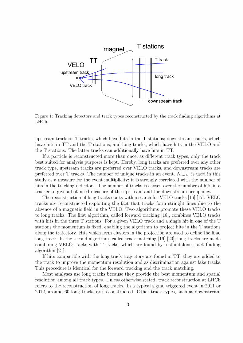
Figure 1: Tracking detectors and track types reconstructed by the track finding algorithms atLHCb.

upstream trackers; T tracks, which have hits in the T stations; downstream tracks, whichhave hits in TT and the T stations; and long tracks, which have hits in the VELO andthe T stations. The latter tracks can additionally have hits in TT.

If a particle is reconstructed more than once, as different track types, only the trackbest suited for analysis purposes is kept. Hereby, long tracks are preferred over any othertrack type, upstream tracks are preferred over VELO tracks, and downstream tracks arepreferred over T tracks. The number of unique tracks in an event, Ntrack, is used in thisstudy as a measure for the event multiplicity; it is strongly correlated with the number ofhits in the tracking detectors. The number of tracks is chosen over the number of hits in atracker to give a balanced measure of the upstream and the downstream occupancy.

The reconstruction of long tracks starts with a search for VELO tracks [16] [17]. VELOtracks are reconstructed exploiting the fact that tracks form straight lines due to theabsence of a magnetic field in the VELO. Two algorithms promote these VELO tracksto long tracks. The first algorithm, called forward tracking [18], combines VELO trackswith hits in the three T stations. For a given VELO track and a single hit in one of the Tstations the momentum is fixed, enabling the algorithm to project hits in the T stationsalong the trajectory. Hits which form clusters in the projection are used to define the finallong track. In the second algorithm, called track matching [19] [20], long tracks are madecombining VELO tracks with T tracks, which are found by a standalone track findingalgorithm [21].

If hits compatible with the long track trajectory are found in TT, they are added tothe track to improve the momentum resolution and as discrimination against fake tracks.This procedure is identical for the forward tracking and the track matching.

Most analyses use long tracks because they provide the best momentum and spatialresolution among all track types. Unless otherwise stated, track reconstruction at LHCbrefers to the reconstruction of long tracks. In a typical signal triggered event in 2011 or2012, around 60 long tracks are reconstructed. Other track types, such as downstream

3

tracks [22], are used for the reconstruction of decay products of long-lived particles suchas K0

S mesons, or for internal alignment of the tracking detectors. They are reconstructedfrom T tracks, which are propagated back through the magnetic field to find correspondinghits in the TT stations.

The efficiency to reconstruct charged particles as long tracks is determined in twoapproaches. The first approach measures the track reconstruction efficiency in the VELOand in the T stations individually and combines these efficiencies to a single measurement.The second approach determines the efficiency to reconstruct a long track directly.

4 Tag-and-probe methods

The tag-and-probe method uses two-prong decays, where one of the decay products, the“tag”, is fully reconstructed as a long track, while the other particle, the “probe”, isonly partially reconstructed. The probe should carry enough momentum informationthat the invariant mass of the parent particle can be reconstructed with a sufficientlyhigh resolution. The invariant mass of the two-prong decay allows for a discriminationagainst background. The track reconstruction efficiency for long tracks is then obtained bymatching the partially reconstructed probe track to a long track. If a match is found, theprobe track is defined as efficient. The three methods described below all use J/ψ → µ+µ−

decays, as the daughter particles have information in the muon system which can beexploited in the reconstruction of the probe track. The approaches, however, use differentcombinations of tracking detectors for the partial reconstruction of the probe track.

4.1 VELO method

The track reconstruction efficiency in the VELO is measured using downstream tracks asprobes, as illustrated in Fig. 2(a). A downstream track and a long track of the same muondo not necessarily share all hits in the T stations. Therefore, a probe track is consideredto be found as a long track if there is a long track with at least 50% common hits inthe T stations. In simulated events the fraction of 50% common hits is found to be anappropriate and stable matching criterion.

4.2 T-station method

The measurement of the track reconstruction efficiency in the T stations for particlesthat have VELO and muon segments is illustrated in Fig. 2(b). A dedicated algorithmreconstructs muons as straight tracks starting from hits in the last muon station, see forexample Refs. [23,24]. These are subsequently matched to VELO tracks.

A long track is considered to be matched to a probe track if two requirements aremet. Firstly, the probe track and the long track have to be reconstructed from the sameVELO seed. Secondly, at least two hits on the probe track in the muon stations have tobe compatible with the extrapolation of the long track into the muon stations. It is found

4

(a)

(b)

(c)

Figure 2: Illustration of the three tag-and-probe methods: (a) the VELO method, (b) theT-station method, and (c) the long method. The VELO (black rectangle), the two TT layers(short bold lines), the magnet coil, the three T stations (long bold lines), and the five muonstations (thin lines) are shown in all three subfigures. The upper solid blue line indicates the tagtrack, the lower line indicates the probe with red dots where hits are required and dashes wherea detector is probed.

in simulated events that requiring two common hits in the muon stations is sufficient toensure compatible trajectories of the long track and the VELO-muon probe track.

5

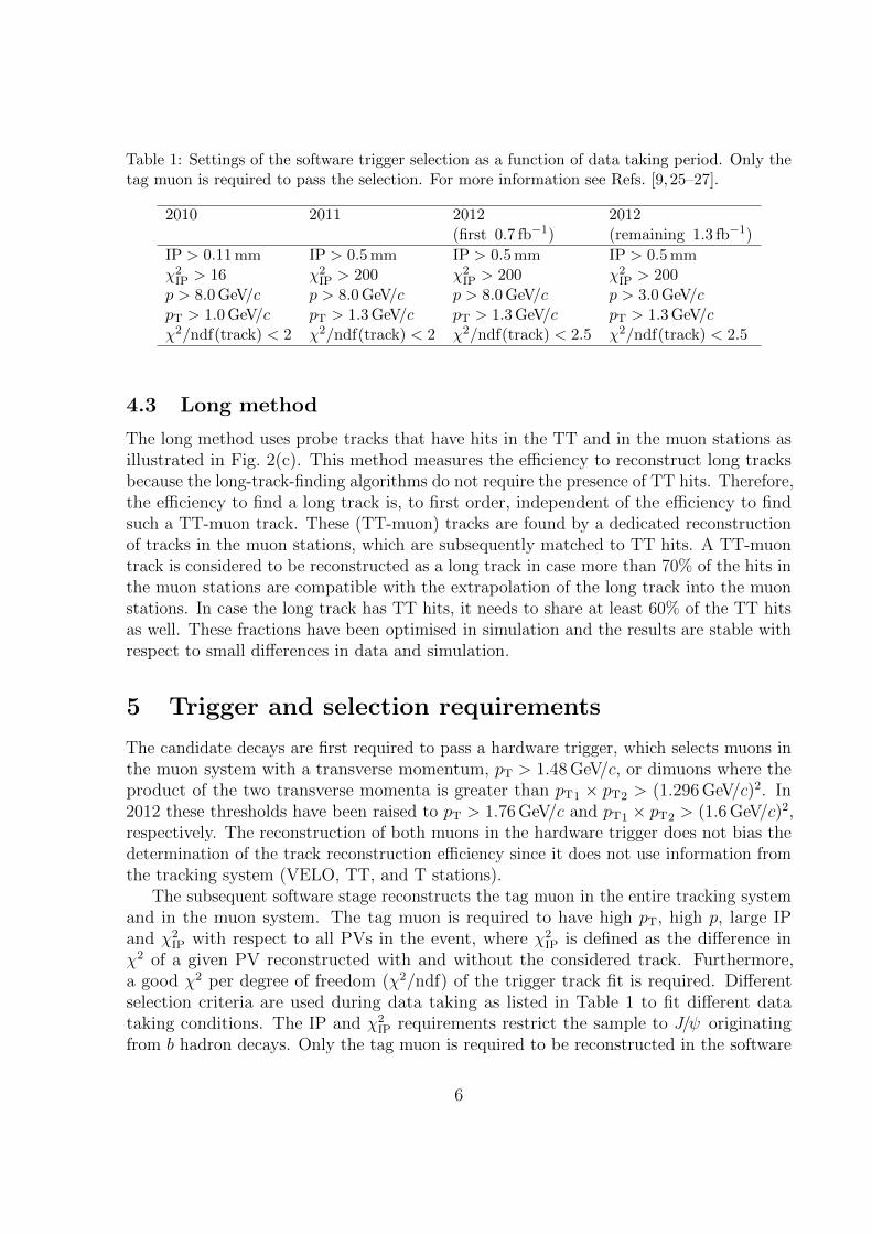
Table 1: Settings of the software trigger selection as a function of data taking period. Only thetag muon is required to pass the selection. For more information see Refs. [9, 25–27].

2010 2011 2012 2012(first 0.7 fb−1) (remaining 1.3 fb−1)

IP > 0.11 mm IP > 0.5 mm IP > 0.5 mm IP > 0.5 mmχ2IP > 16 χ2

IP > 200 χ2IP > 200 χ2

IP > 200p > 8.0 GeV/c p > 8.0 GeV/c p > 8.0 GeV/c p > 3.0 GeV/cpT > 1.0 GeV/c pT > 1.3 GeV/c pT > 1.3 GeV/c pT > 1.3 GeV/cχ2/ndf(track) < 2 χ2/ndf(track) < 2 χ2/ndf(track) < 2.5 χ2/ndf(track) < 2.5

4.3 Long method

The long method uses probe tracks that have hits in the TT and in the muon stations asillustrated in Fig. 2(c). This method measures the efficiency to reconstruct long tracksbecause the long-track-finding algorithms do not require the presence of TT hits. Therefore,the efficiency to find a long track is, to first order, independent of the efficiency to findsuch a TT-muon track. These (TT-muon) tracks are found by a dedicated reconstructionof tracks in the muon stations, which are subsequently matched to TT hits. A TT-muontrack is considered to be reconstructed as a long track in case more than 70% of the hits inthe muon stations are compatible with the extrapolation of the long track into the muonstations. In case the long track has TT hits, it needs to share at least 60% of the TT hitsas well. These fractions have been optimised in simulation and the results are stable withrespect to small differences in data and simulation.

5 Trigger and selection requirements

The candidate decays are first required to pass a hardware trigger, which selects muons inthe muon system with a transverse momentum, pT > 1.48 GeV/c, or dimuons where theproduct of the two transverse momenta is greater than pT1 × pT2 > (1.296 GeV/c)2. In2012 these thresholds have been raised to pT > 1.76 GeV/c and pT1 × pT2 > (1.6 GeV/c)2,respectively. The reconstruction of both muons in the hardware trigger does not bias thedetermination of the track reconstruction efficiency since it does not use information fromthe tracking system (VELO, TT, and T stations).

The subsequent software stage reconstructs the tag muon in the entire tracking systemand in the muon system. The tag muon is required to have high pT, high p, large IPand χ2

IP with respect to all PVs in the event, where χ2IP is defined as the difference in

χ2 of a given PV reconstructed with and without the considered track. Furthermore,a good χ2 per degree of freedom (χ2/ndf) of the trigger track fit is required. Differentselection criteria are used during data taking as listed in Table 1 to fit different datataking conditions. The IP and χ2

IP requirements restrict the sample to J/ψ originatingfrom b hadron decays. Only the tag muon is required to be reconstructed in the software

6

Table 2: Selection requirements on the tag and probe tracks and on the combination into a J/ψcandidate for the three different methods.

VELO T-station Longmethod method method

Tag Long trackused in single muon trigger

DLLµπ > 2 DLLµπ > 2χ2/ndf(track) < 5 χ2/ndf(track) < 3 χ2/ndf(track) < 2p > 5.0 GeV/c p > 7.0 GeV/c p > 10 GeV/cpT > 0.7 GeV/c pT > 0.5 GeV/c pT > 1.3 GeV/c

IP > 0.5 mm

Probe Downstream track VELO-muon track TT-muon trackp > 5.0 GeV/c p > 5.0 GeV/c p > 5.0 GeV/cpT > 0.7 GeV/c pT > 0.5 GeV/c pT > 0.1 GeV/c

J/ψ Mµµ ∈ [2.9, 3.3] GeV/c2 Mµµ ∈ [2.7, 3.5] GeV/c2 Mµµ ∈ [2.6, 3.6] GeV/c2

χ2/ndf(vertex) < 5 χ2/ndf(vertex) < 5 χ2/ndf(vertex) < 5NJ/ψ = 1 NJ/ψ = 1 NJ/ψ = 1

p > 7.0 GeV/c IP < 0.8 mm

trigger in order to avoid any bias on the track reconstruction efficiency, caused by fullyreconstructing the two-prong decay with two long tracks.

Further selection criteria are applied as listed in Table 2: the χ2/ndf from the track fitof the tag tracks must be small to reduce the number of fake tracks. Tag tracks have tofulfil the standard muon selection, which requires hits in the muon stations in a searchwindow around the track extrapolation as explained in Ref. [28]. Both the tag and probetracks have minimal p and pT requirements to remove badly reconstructed tracks andcombinatorial background. In order to remove contamination from hadrons, the particleidentification system is used. The differences between the logarithm of the likelihood ofthe tag to be a muon and to be a pion, DLLµπ, is computed and only tag tracks with ahigh DLLµπ are used. The range of the invariant mass of the µ+µ− combination, Mµµ, ischosen sufficiently large to estimate the background contribution from the mass sidebands.Finally, the χ2/ndf from the vertex fit of the tag- and the probe-track has to be small, inorder to remove combinatorial background; and the number of J/ψ decays per event (NJ/ψ )must be one, to simplify the association procedure described in the preceding subsections.Additionally, the T-station method only considers J/ψ candidates with a momentumgreater than 7 GeV/c, and the long method only J/ψ candidates with an IP smaller than0.8 mm, as both selections are effective in reducing background contamination withoutbiasing the efficiency determination. After the full selection chain the sample amounts toabout 6 000 decays for 2010 for the long and the T method, while for the VELO method12 000 decays are selected. The 2011 and 2012 data samples comprise more than 300 000decays in total for all methods and data taking periods.

7

]2c [MeV/−µ+µM2800 3000 3200 3400

)2 cC

andi

date

s / (

4 M

eV/

0

5000

1000015000

20000

25000

30000

35000

40000

45000 LHCb(a)VELO method

]2c [MeV/−µ+µM2800 3000 3200 3400

)2 cC

andi

date

s / (

9.5

MeV

/

0

5000

10000

15000

20000

25000

30000

35000

40000 LHCb(b)T-station method

]2c [MeV/−µ+µM2800 3000 3200 3400

)2 cCa

ndid

ates

/ (7

.5 M

eV/

0

5000

10000

15000

20000

25000

30000LHCb(c)

Long method

]2c [MeV/−µ+µM2800 3000 3200 3400

)2 cC

andi

date

s / (

4 M

eV/

0

10000

20000

30000

40000

50000

60000

70000

80000 LHCb(d)Standard reconstruction

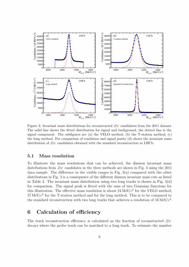
Figure 3: Invariant mass distributions for reconstructed J/ψ candidates from the 2011 dataset.The solid line shows the fitted distribution for signal and background, the dotted line is thesignal component. The subfigures are (a) the VELO method, (b) the T-station method, (c)the long method. For comparison of resolution and signal purity (d) shows the invariant massdistribution of J/ψ candidates obtained with the standard reconstruction at LHCb.

5.1 Mass resolution

To illustrate the mass resolutions that can be achieved, the dimuon invariant massdistributions from J/ψ candidates in the three methods are shown in Fig. 3 using the 2011data sample. The difference in the visible ranges in Fig. 3(a) compared with the otherdistributions in Fig. 3 is a consequence of the different dimuon invariant mass cuts as listedin Table 2. The invariant mass distribution using two long tracks is shown in Fig. 3(d)for comparison. The signal peak is fitted with the sum of two Gaussian functions forthis illustration. The effective mass resolution is about 24 MeV/c2 for the VELO method,57 MeV/c2 for the T-station method and for the long method. This is to be compared tothe standard reconstruction with two long tracks that achieves a resolution of 16 MeV/c2.

6 Calculation of efficiency

The track reconstruction efficiency is calculated as the fraction of reconstructed J/ψdecays where the probe track can be matched to a long track. To estimate the number

8

of J/ψ decays, an unbinned extended maximum likelihood fit is performed to the massdistributions. For the VELO and T-station methods the mass distributions are described bya single Gaussian function for the signal and an exponential function for the combinatorialbackground. This model is preferred over the aforementioned sum of two Gaussian functionsto improve the fit stability when measuring the dependence of the track reconstructionefficiency on kinematic variables and other event parameters. For the long method, aCrystal Ball function [29] is used for the signal, to take the tail on the left-hand side ofthe mass peak into account. Since the number of decays in the 2010 data is relativelylow, in this case a simple sideband subtraction is applied for the VELO and T-stationmethods. All shape parameters were allowed to vary in the fit for the denominator of theefficiency; they were constrained to the found values for the numerator of the efficiency.This procedure was performed to stabilise the fit, as no difference in the shape of thenumerator and denominator could be observed. It has been checked that the choice of themodel for the mass distribution has a negligible effect on the efficiency determination.

The efficiencies obtained from the VELO and T-station methods are assumed to beuncorrelated, aside from effects due to dependencies on the track kinematics and the eventmultiplicity. The data sample is binned in kinematic variables and Ntrack to combine theVELO and T-station efficiencies. The efficiencies obtained with the VELO and T-stationmethods can be multiplied in each bin to obtain the efficiency for finding long tracks. Thiscombined efficiency can be compared with the efficiency found by the long method, givingtwo independent methods to probe the long track reconstruction efficiency.

There are, however, small differences between these two approaches. The long methodmeasures the efficiency for tracks that pass through TT. In the combined method, only theVELO method requires this. Furthermore, both the VELO method and T-station methodinclude the efficiency that, given that both the VELO and the T-station segment tracks arereconstructed, the corresponding long track is found. Therefore, in the combined efficiency,this so-called matching efficiency is counted twice. All these effects can lead to smalldifferences in the measured long-track efficiency. For this reason, the ratio between theefficiencies in data and simulation is used to compare the methods, as these uncertaintiesare common for simulated and real decays and cancel when the ratio of efficiencies isformed.

On simulated events the track reconstruction efficiency is commonly defined as thefraction of simulated charged particles with sufficient hits in the VELO and T stationsthat can be associated to a track that shares at least 70% of the hits in each participatingsubdetector with this particle. For all methods, this so-called hit-based efficiency insimulation agrees within 1% with the efficiency measured with the tag-and-probe methods.Furthermore the matching efficiency was determined to be very close to 100%. The verysmall matching inefficiency does not affect the agreement between the hit-based efficiencyand the tag-and-probe based efficiency in simulation. By taking the ratio between theefficiencies on data and simulation, these discrepancies are reduced to a negligible level.

9

Table 3: Track reconstruction efficiencies in % for the individual running periods using thelong method for positive and negative muons and different magnetic field polarities (statisticaluncertainties only).

Magnet up Magnet downData Positive Negative Positive Negative

2010 94.1± 1.3 96.0± 1.3 99.3+0.7−1.8 98.4+1.6

−1.72011 97.0± 0.3 97.3± 0.3 97.2± 0.3 97.4± 0.32012 96.2± 0.2 96.2± 0.2 96.2± 0.2 96.3± 0.2

7 Efficiency dependencies

Using the momentum spectrum of the J/ψ decay products obtained with the VELOmethod from data as a benchmark, the average track reconstruction efficiency for longtracks is measured to be (95.4± 0.7)% for 2010 data, (97.78± 0.07)% for 2011 data and(96.99 ± 0.05)% for 2012 data. All results confirm the good performance of the LHCbtracking system. The uncertainties on these numbers are statistical only; they are binomialerrors with additional terms to account for the statistical uncertainty on the number ofbackground events. Systematic uncertainties are discussed in Sect. 8. The difference in theefficiencies between the three years is a consequence of changes in the track reconstructionand the higher centre-of-mass energy, leading to a higher track multiplicity and hence lowerreconstruction efficiency for the 2012 running period. Dependencies on the polarity of thedipole magnet, the charge of the muons, and kinematic properties as well as the agreementwith the simulation are investigated in further detail in the following subsections.

7.1 Comparison of magnetic field polarities

The track reconstruction efficiencies determined from the long method are split up intopositively and negatively charged muons and into the two different magnetic field polarities(named up and down). The results are summarised in Table 3. They show compatiblenumbers for magnetic field up and down and for positive and negative muons.

For data from 2011 and 2012 there is no difference between positive and negativemuons or between the different magnet polarities. In 2010 data, a 2.3σ difference betweenthe different magnet polarities is observed for positive muons. No unambiguous source ofthe difference is found.

7.2 Dependencies of track reconstruction efficiency

The efficiency to reconstruct long tracks mainly depends on the particle kinematics and thenumber of charged particles in an event. As a parametrisation p, η and Ntrack are chosen, asthe track reconstruction efficiency shows the largest dependence on these three observables.The simulated events are weighted according to the Ntrack distribution observed in data.

10

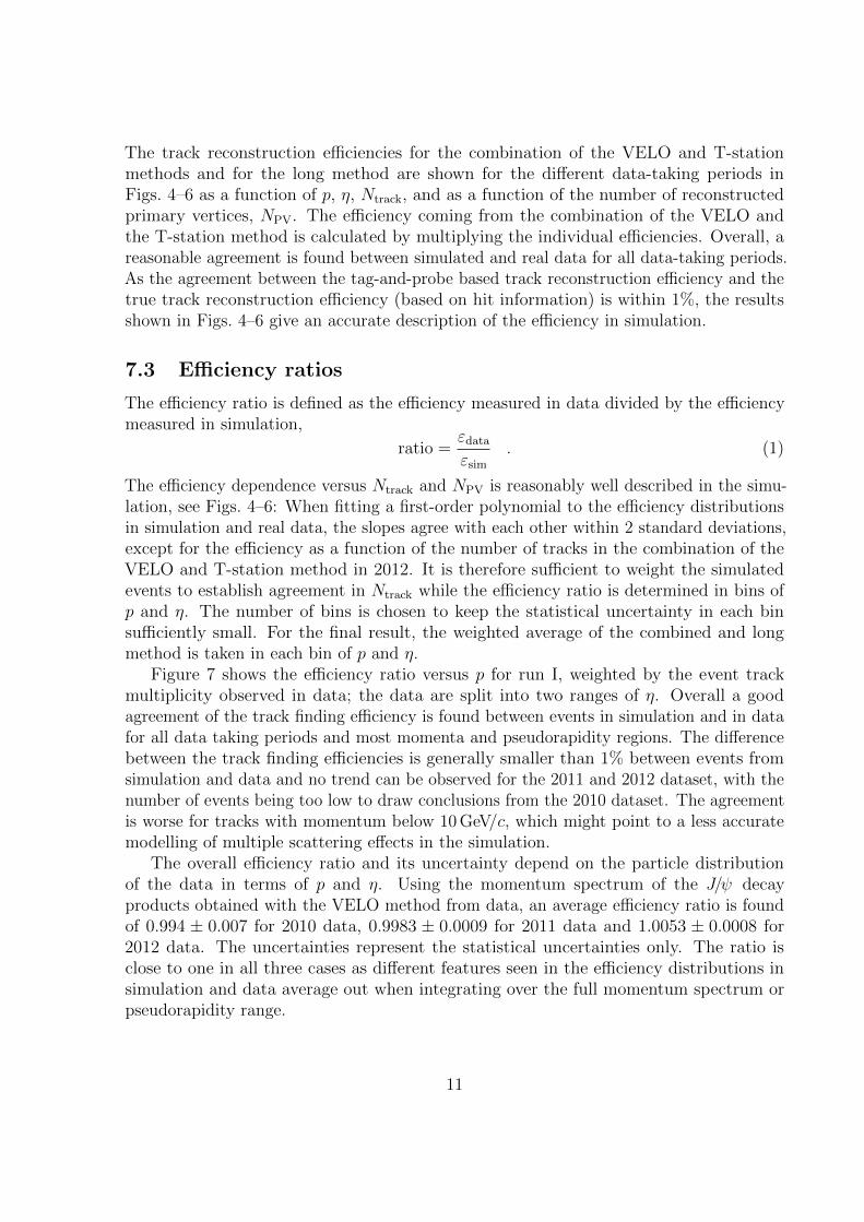
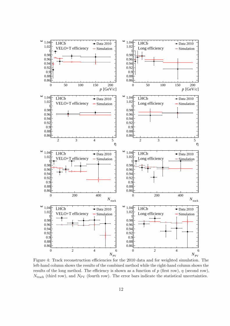
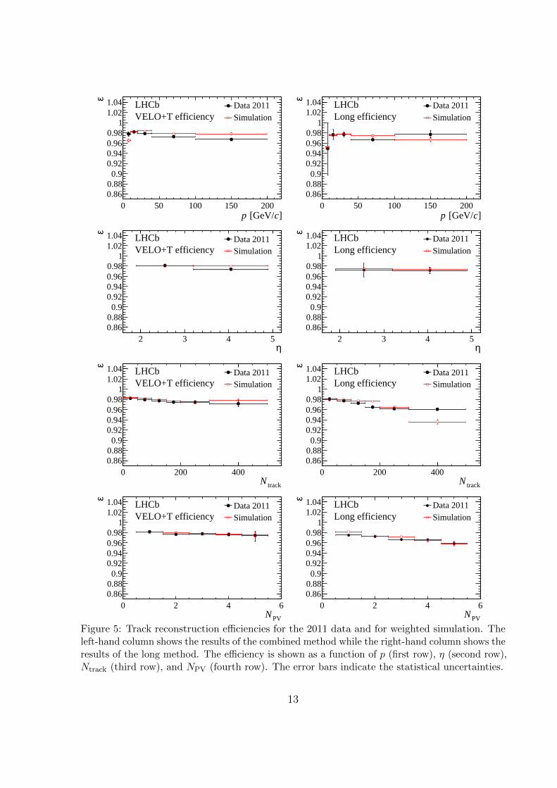
The track reconstruction efficiencies for the combination of the VELO and T-stationmethods and for the long method are shown for the different data-taking periods inFigs. 4–6 as a function of p, η, Ntrack, and as a function of the number of reconstructedprimary vertices, NPV. The efficiency coming from the combination of the VELO andthe T-station method is calculated by multiplying the individual efficiencies. Overall, areasonable agreement is found between simulated and real data for all data-taking periods.As the agreement between the tag-and-probe based track reconstruction efficiency and thetrue track reconstruction efficiency (based on hit information) is within 1%, the resultsshown in Figs. 4–6 give an accurate description of the efficiency in simulation.

7.3 Efficiency ratios

The efficiency ratio is defined as the efficiency measured in data divided by the efficiencymeasured in simulation,

ratio =εdataεsim

. (1)

The efficiency dependence versus Ntrack and NPV is reasonably well described in the simu-lation, see Figs. 4–6: When fitting a first-order polynomial to the efficiency distributionsin simulation and real data, the slopes agree with each other within 2 standard deviations,except for the efficiency as a function of the number of tracks in the combination of theVELO and T-station method in 2012. It is therefore sufficient to weight the simulatedevents to establish agreement in Ntrack while the efficiency ratio is determined in bins ofp and η. The number of bins is chosen to keep the statistical uncertainty in each binsufficiently small. For the final result, the weighted average of the combined and longmethod is taken in each bin of p and η.

Figure 7 shows the efficiency ratio versus p for run I, weighted by the event trackmultiplicity observed in data; the data are split into two ranges of η. Overall a goodagreement of the track finding efficiency is found between events in simulation and in datafor all data taking periods and most momenta and pseudorapidity regions. The differencebetween the track finding efficiencies is generally smaller than 1% between events fromsimulation and data and no trend can be observed for the 2011 and 2012 dataset, with thenumber of events being too low to draw conclusions from the 2010 dataset. The agreementis worse for tracks with momentum below 10 GeV/c, which might point to a less accuratemodelling of multiple scattering effects in the simulation.

The overall efficiency ratio and its uncertainty depend on the particle distributionof the data in terms of p and η. Using the momentum spectrum of the J/ψ decayproducts obtained with the VELO method from data, an average efficiency ratio is foundof 0.994 ± 0.007 for 2010 data, 0.9983 ± 0.0009 for 2011 data and 1.0053 ± 0.0008 for2012 data. The uncertainties represent the statistical uncertainties only. The ratio isclose to one in all three cases as different features seen in the efficiency distributions insimulation and data average out when integrating over the full momentum spectrum orpseudorapidity range.

11

]c [GeV/p0 50 100 150 200

ε

0.860.880.9

0.920.940.960.98

11.021.04 Data 2010

Simulation

LHCbVELO+T efficiency

]c [GeV/p0 50 100 150 200

ε

0.860.880.9

0.920.940.960.98

11.021.04 Data 2010

Simulation

LHCbLong efficiency

η2 3 4 5

ε

0.860.880.9

0.920.940.960.98

11.021.04 Data 2010

Simulation

LHCbVELO+T efficiency

η2 3 4 5

ε

0.860.880.9

0.920.940.960.98

11.021.04 Data 2010

Simulation

LHCbLong efficiency

trackN0 200 400

ε

0.860.880.9

0.920.940.960.98

11.021.04 Data 2010

Simulation

LHCbVELO+T efficiency

trackN0 200 400

ε

0.860.880.9

0.920.940.960.98

11.021.04 Data 2010

Simulation

LHCbLong efficiency

PVN0 2 4 6

ε

0.860.880.9

0.920.940.960.98

11.021.04 Data 2010

Simulation

LHCbVELO+T efficiency

PVN0 2 4 6

ε

0.860.880.9

0.920.940.960.98

11.021.04 Data 2010

Simulation

LHCbLong efficiency

Figure 4: Track reconstruction efficiencies for the 2010 data and for weighted simulation. Theleft-hand column shows the results of the combined method while the right-hand column shows theresults of the long method. The efficiency is shown as a function of p (first row), η (second row),Ntrack (third row), and NPV (fourth row). The error bars indicate the statistical uncertainties.

12

]c [GeV/p0 50 100 150 200

ε

0.860.880.9

0.920.940.960.98

11.021.04 Data 2011

Simulation

LHCbVELO+T efficiency

]c [GeV/p0 50 100 150 200

ε

0.860.880.9

0.920.940.960.98

11.021.04 Data 2011

Simulation

LHCbLong efficiency

η2 3 4 5

ε

0.860.880.9

0.920.940.960.98

11.021.04 Data 2011

Simulation

LHCbVELO+T efficiency

η2 3 4 5

ε

0.860.880.9

0.920.940.960.98

11.021.04 Data 2011

Simulation

LHCbLong efficiency

trackN0 200 400

ε

0.860.880.9

0.920.940.960.98

11.021.04 Data 2011

Simulation

LHCbVELO+T efficiency

trackN0 200 400

ε

0.860.880.9

0.920.940.960.98

11.021.04 Data 2011

Simulation

LHCbLong efficiency

PVN0 2 4 6

ε

0.860.880.9

0.920.940.960.98

11.021.04 Data 2011

Simulation

LHCbVELO+T efficiency

PVN0 2 4 6

ε

0.860.880.9

0.920.940.960.98

11.021.04 Data 2011

Simulation

LHCbLong efficiency

Figure 5: Track reconstruction efficiencies for the 2011 data and for weighted simulation. Theleft-hand column shows the results of the combined method while the right-hand column shows theresults of the long method. The efficiency is shown as a function of p (first row), η (second row),Ntrack (third row), and NPV (fourth row). The error bars indicate the statistical uncertainties.

13

]c [GeV/p0 50 100 150 200

ε

0.860.880.9

0.920.940.960.98

11.021.04 Data 2012

Simulation

LHCbVELO+T efficiency

]c [GeV/p0 50 100 150 200

ε

0.860.880.9

0.920.940.960.98

11.021.04 Data 2012

Simulation

LHCbLong efficiency

η2 3 4 5

ε

0.860.880.9

0.920.940.960.98

11.021.04 Data 2012

Simulation

LHCbVELO+T efficiency

η2 3 4 5

ε

0.860.880.9

0.920.940.960.98

11.021.04 Data 2012

Simulation

LHCbLong efficiency

trackN0 200 400

ε

0.860.880.9

0.920.940.960.98

11.021.04 Data 2012

Simulation

LHCbVELO+T efficiency

trackN0 200 400

ε

0.860.880.9

0.920.940.960.98

11.021.04 Data 2012

Simulation

LHCbLong efficiency

PVN0 2 4 6

ε

0.860.880.9

0.920.940.960.98

11.021.04 Data 2012

Simulation

LHCbVELO+T efficiency

PVN0 2 4 6

ε

0.860.880.9

0.920.940.960.98

11.021.04 Data 2012

Simulation

LHCbLong efficiency

Figure 6: Track reconstruction efficiencies for the 2012 data and for weighted simulation. Theleft-hand column shows the results of the combined method while the right-hand column shows theresults of the long method. The efficiency is shown as a function of p (first row), η (second row),Ntrack (third row), and NPV (fourth row). The error bars indicate the statistical uncertainties.

14

]c [GeV/p10 210

Eff

icie

ncy

ratio

0.9

0.95

1

1.05

1.1 <3.2η1.9<<4.9η3.2<

LHCbData/Simulation 2010

]c [GeV/p10 210

Eff

icie

ncy

ratio

0.9

0.95

1

1.05

1.1 <3.2η1.9<<4.9η3.2<

LHCbData/Simulation 2011

]c [GeV/p10 210

Eff

icie

ncy

ratio

0.9

0.95

1

1.05

1.1 <3.2η1.9<<4.9η3.2<

LHCbData/Simulation 2012

Figure 7: Track reconstruction efficiency ratios as a function of p between data and simulationfor (left) 2010 data, (right) 2011 data, and (bottom) 2012 data.

8 Systematic uncertainties

Small differences in the ratio of efficiencies are seen when reweighting the simulatedsamples in different parameters such as the number of primary vertices, or the number ofhits or tracks in the different subdetectors. The largest of these differences is taken asa systematic uncertainty and amounts to 0.4%. No systematic uncertainty is assignedfor the agreement of the track reconstruction efficiency determined by the tag-and-probemethod and the hit-based method (which is on the order of 1%), as the differences cancelwhen forming the efficiency ratio. Accordingly, no systematic uncertainties are assignedfor the fit model as these cancel when forming the fraction of reconstructed J/ψ decayswhere the probe can be matched to a long track. It has been checked that this is truefor a range of fit models, the largest variation being 0.2%. Furthermore, no systematicuncertainty is assigned to the possible matching of a correctly reconstructed probe trackto a fake long track, as the requirement for a large overlap in the subdetectors ensure thatboth reconstructed tracks are either real tracks or fake tracks, where the latter would notpeak at the J/ψ mass. No systematic uncertainty is assigned for the fact that the VELO+ T-station method and the long method show slightly different results in Figs. 4–6, asboth methods probe different momentum spectra and any residual difference will cancel

15

when forming the ratio with simulation. No systematic uncertainty is assigned for thedouble-counting of the matching efficiency in the combined method, as this efficiency isvery close to 100%, and any uncertainty would get further reduced when forming the ratiowith simulation. No systematic uncertainty is assigned for the large difference for theVELO + T efficiency between simulation and data at low momenta in 2011 and 2012, asthis is automatically taken into account when forming the ratio of efficiencies. Despite thisdifference, the integrated track reconstruction efficiencies between simulation and data arein agreement due to compensation of this effect for high momenta, where the efficiency ishigher in simulation than in data.

9 Hadronic interactions

The methods presented in this paper are based on muons and require that they reachthe muon stations. Thus, these methods are not sensitive to the effects from hadronicinteractions and large-angle scatterings with the detector material. For hadrons, the largesteffect is due to hadronic interactions. The cross section depends on the particle type, chargeand the momentum. A simulation of B0 → J/ψK∗0 decays (where K∗0 → K+π−) showsthat about 11% of the kaons (averaged over positive and negative kaons) and about 14% ofthe pions cannot be reconstructed due to hadronic interactions that occur before the lastT station. This number depends primarily on the momentum of the particle. Due to theuncertainty on the material budget and consequently on the interaction with the detectormaterial, the reconstruction efficiency obtained from simulation has an intrinsic uncertainty,which is not accounted for in the track reconstruction efficiencies measured with muons.When assuming that the total material budget in the simulation has an uncertainty of10%, the systematic uncertainty due to hadronic interactions is between 1.1–1.4%. The10% uncertainty is used as a conservative upper limit and is composed as follows: for theVELO a calculation in Ref. [4] shows an uncertainty on the material budget of 6%. Nodirect measurements exist for the T and TT stations. However, weight measurementsfor the Inner Tracker for the silicon sensors and the detector boxes give an accuracy of2%, while an agreement of 5% is reached for the cables and the support structure [30, 31].The Outer Tracker modules have been weighted and this measurement is precise to about1% [32]. Furthermore, the sum of the weights of the individual components of a moduleadds up to the total weight of a module within the uncertainties. Taking into account thatsome level of detail is missing in the detector description in the simulation, an uncertaintyof 5% is assumed for the outer tracker. Weight measurements for the sensor modulesand the insulation material of TT have been performed. Given the detail of the detectordescription [33] an uncertainty of 5% on the material budget is well justified. The beam-pipe was implemented in the software following the design drawings, where a precisionbetter than 10% for all pieces was confirmed following measurements after production.The solid radiator (aerogel) and the gas radiator (C4F10) contribute more than two-thirdof the material budget for the RICH1 detector [34]. The amount of aerogel is known up to2% and the differences between 2011 and 2012 are accounted for in the simulation. The

16

density of the C4F10 was monitored, with the RMS of the distribution being about 1%.The other components of RICH1 have a smaller contribution to the interaction length.The overall uncertainty of 10% for the full material budget was then chosen to also takeuncertainties on the Geant4 cross-sections and additional uncertainties, coming fromsimplified descriptions of the detector elements in the simulation, into account.

10 Conclusion

Track reconstruction efficiencies at LHCb have been measured using a tag-and-probemethod with J/ψ → µ+µ− decays. The average efficiency is better than 95% in themomentum region 5 GeV/c < p < 200 GeV/c and in the pseudorapidity region 2 < η < 5,which covers the phase space of LHCb. The uncertainty per track is below 0.5% for muonsand below 1.5% for pions and kaons, where the larger uncertainty takes the uncertaintyon hadronic interactions into account. All uncertainties have been added in quadrature.Furthermore, the ratio of the track reconstruction efficiency of muons in data and simulationis measured, where an uncertainty of 0.8 % for data collected in 2010 and an uncertainty of0.4 % for data collected in 2011 and 2012 is achieved. The integrated efficiency ratios forall three years of data taking are compatible with unity. This result presents a significantimprovement over the uncertainties determined with previous methods ranging from 3 to4%.

Acknowledgements

We express our gratitude to our colleagues in the CERN accelerator departments for theexcellent performance of the LHC. We thank the technical and administrative staff at theLHCb institutes. We acknowledge support from CERN and from the national agencies:CAPES, CNPq, FAPERJ, and FINEP (Brazil); NSFC (China); CNRS/IN2P3 (France);BMBF, DFG, HGF, and MPG (Germany); SFI (Ireland); INFN (Italy); FOM and NWO(The Netherlands); MNiSW and NCN (Poland); MEN/IFA (Romania); MinES and FANO(Russia); MinECo (Spain); SNSF and SER (Switzerland); NASU (Ukraine); STFC (UnitedKingdom); NSF (USA). The Tier1 computing centres are supported by IN2P3 (France),KIT and BMBF (Germany), INFN (Italy), NWO and SURF (The Netherlands), PIC(Spain), GridPP (United Kingdom). We are indebted to the communities behind themultiple open source software packages on which we depend. We are also thankful forthe computing resources and the access to software R&D tools provided by Yandex LLC(Russia). Individual groups or members have received support from EPLANET, MarieSk lodowska-Curie Actions, and ERC (European Union), Conseil general de Haute-Savoie,Labex ENIGMASS, and OCEVU, Region Auvergne (France), RFBR (Russia), XuntaGal,and GENCAT (Spain), Royal Society and Royal Commission for the Exhibition of 1851(United Kingdom).

17

References

[1] LHCb collaboration, R. Aaij et al., Measurement of σ(pp→ bbX) at√s = 7 TeV in

the forward region, Phys. Lett. B694 (2010) 209, arXiv:1009.2731.

[2] LHCb collaboration, R. Aaij et al., Production of J/ψ and Υ mesons in pp collisionsat√s = 8 TeV, JHEP 06 (2013) 064, arXiv:1304.6977.

[3] LHCb collaboration, A. A. Alves Jr. et al., The LHCb detector at the LHC, JINST 3(2008) S08005.

[4] R. Aaij et al., Performance of the LHCb Vertex Locator, JINST 9 (2014) 09007,arXiv:1405.7808.

[5] LHCb collaboration, LHCb reoptimized detector design and performance: TechnicalDesign Report, CERN-LHCC-2003-030. LHCB-TDR-009.

[6] LHCb collaboration, LHCb inner tracker: Technical Design Report, CERN-LHCC-2002-029. LHCB-TDR-008.

[7] R. Arink et al., Performance of the LHCb Outer Tracker, JINST 9 (2014) P01002,arXiv:1311.3893.

[8] A. A. Alves Jr. et al., Performance of the LHCb muon system, JINST 8 (2013) P02022,arXiv:1211.1346.

[9] R. Aaij et al., The LHCb trigger and its performance in 2011, JINST 8 (2013) P04022,arXiv:1211.3055.

[10] T. Sjostrand, S. Mrenna, and P. Skands, PYTHIA 6.4 physics and manual, JHEP 05(2006) 026, arXiv:hep-ph/0603175.

[11] I. Belyaev et al., Handling of the generation of primary events in Gauss, the LHCbsimulation framework, Nuclear Science Symposium Conference Record (NSS/MIC)IEEE (2010) 1155.

[12] D. J. Lange, The EvtGen particle decay simulation package, Nucl. Instrum. Meth.A462 (2001) 152.

[13] P. Golonka and Z. Was, PHOTOS Monte Carlo: a precision tool for QED correctionsin Z and W decays, Eur. Phys. J. C45 (2006) 97, arXiv:hep-ph/0506026.

[14] Geant4 collaboration, J. Allison et al., Geant4 developments and applications, IEEETrans. Nucl. Sci. 53 (2006) 270; Geant4 collaboration, S. Agostinelli et al., Geant4: asimulation toolkit, Nucl. Instrum. Meth. A506 (2003) 250.

[15] M. Clemencic et al., The LHCb simulation application, Gauss: design, evolution andexperience, J. Phys. Conf. Ser. 331 (2011) 032023.

18

[16] D. Hutchcroft, VELO pattern recognition, CERN-LHCB-2007-013.

[17] O. Callot, FastVelo, a fast and efficient pattern recognition package for the Velo,LHCb-PUB-2011-001, CERN-LHCb-PUB-2011-001.

[18] O. Callot and S. Hansmann-Menzemer, The Forward Tracking, LHCb-2007-015,CERN-LHCb-2007-015.

[19] M. Needham and J. Van Tilburg, Performance of the track matching, LHCb-2007-020,CERN-LHCb-2007-020.

[20] M. Needham, Performance of the track matching, CERN-LHCB-2007-129.

[21] O. Callot and M. Schiller, PatSeeding: A standalone track reconstruction algorithm,CERN-LHCB-2008-042.

[22] O. Callot, Downstream pattern recognition, CERN-LHCB-2007-026.

[23] G. Manca, L. Mou, and B. Saitta, Studies of Efficiency of the LHCb Muon DetectorUsing Cosmic Rays, LHCb-PUB-2009-017.

[24] G. Passaleva, A recurrent neural network for track reconstruction in the LHCb MuonSystem, Nuclear Science Symposium Conference Record, 2008. NSS ’08. IEEE (2008)867 .

[25] J. Albrecht, L. de Paula, A. Perez-Calero Yzquierdo, and F. Teubert, Commissioningand Performance of the LHCb HLT1 muon trigger, LHCb-PUB-2011-006.

[26] V. V. Gligorov, A single track HLT1 trigger, LHCb-PUB-2011-003.

[27] J. Albrecht, V. Gligorov, G. Raven, and S. Tolk, Performance of the LHCb High LevelTrigger in 2012, arXiv:1310.8544.

[28] F. Archilli et al., Performance of the muon identification at LHCb, JINST 8 (2013)P10020, arXiv:1306.0249.

[29] T. Skwarnicki, A study of the radiative cascade transitions between the Upsilon-primeand Upsilon resonances, PhD thesis, Institute of Nuclear Physics, Krakow, 1986,DESY-F31-86-02.

[30] V. Fave, Estimation of the material budget of the Inner Tracker, LHCb-2008-054,CERN-LHCb-2008-054.

[31] V. Fave, Survey of the Cables of the Inner Tracker, LHCb-2008-055, CERN-LHCb-2008-055.

[32] J. Nardulli and N. Tuning, A Study of the Material in an Outer Tracker Module,LHCb-2004-114, CERN-LHCb-2004-114.

19

[33] C. Salzmann and J. Van Tilburg, TT detector description and implementation of thesurvey measurements, LHCb-2008-061, CERN-LHCb-2008-061.

[34] LHCb RICH Collaboration, N. Brook et al., LHCb RICH1 Engineering Design ReviewReport, LHCb-2004-121. CERN-LHCb-2004-121.

20