Embed Size (px)
Citation preview
/tr Università degli studi di GenovaFacoltà di scienze Matematiche, Fisiche e Naturali
Scuola di Dottorato in Scienze e Tecnologieper l’informazione e la conoscenza
XXIV Ciclo, A.A. 2009 - 2012
A Thesis submitted for the degree ofDottore di Ricerca in
Fisica
Measurement of the pep and CNO solarneutrino interaction rates in Borexino
AuthorStefano Davini
Università e sezione INFN di Genova
School CoordinatorProf. Lorenzo MatteraUniversità degli Studi di Genova
AdvisorProf. Marco PallaviciniUniversità e sezione INFN di Genova
External AdvisorProf. Cristiano Galbiati
Princeton University
Area 02 - Scienze FisicheSettore Scientifico-Disciplinare: 02/A1


Introduction
All matter around us is mainly constituted by three particles: protons and neutrons,which make up the atomic nucleus, and electrons, which form the atomic shell. TheUniverse, however, reveals a great deal of other particles, present from its very beginning,immediately after the Big Bang. Among the still existing particles, one of the strangestand most elusive is the neutrino.
Neutrinos (ν) are neutral particles with a very low mass, which permeate the Universeand are constantly produced in many processes involving radioactive decays as well asnuclear fusion in stars. The most powerful neutrino source near the Earth is the Sun.In the core of the Sun, a series of nuclear reactions produce neutrinos. Two distinctprocesses, the main proton-proton (pp) fusion chain and the sub-dominants carbon-nitrogen-oxygen (CNO) cycle, are responsible for the solar energy production. In suchprocesses, electron neutrinos (νe) with different energy spectra and fluxes are generated.The Sun is producing a great amount of neutrinos: the solar neutrino flux at the Earthdistance is about 6× 1010 cm−2s−1.
Because neutrino interact only via the weak interaction, they can easily penetratehuge thicknesses of matter while keeping their original features, thus allowing the studyof phenomena directly connected to their origin. Indeed, while photons produced in thefusion take some hundred thousand years to travel across the 7 × 10⁵ km solar radius,neutrinos take a bit more than 2 seconds. After an additional 8 minutes they reach theEarth, providing precious information concerning energy production processes in theSun and stars in general.
Since 1970’s, solar neutrino experiments have proved to be sensitive tools to test bothastrophysical and elementary particle physics models. The experimental observation ofneutrinos is extremely complex due to the very low interaction rates of the neutrinowith matter. In order to face this problem, huge experimental detectors have beenrealized and placed in underground areas to avoid the background generated by cosmicrays. Solar neutrino detectors were first built to demonstrate that the sun is poweredby nuclear fusion reactions. Until mid 2011, only 7Be (from the reaction e− + 7Be →7Li + νe), 8B (from the reaction 8B → 8Be + e+ + νe), and indirectly pp (from thereaction p + p → 2H + e+ + νe) solar neutrino fluxes from the proton-proton chainhave been measured.
The number of solar νe observed in the experiments carried out for several years hasalways been lower than the one predicted by the astrophysical model which describe thebehaviour of the Sun, the Standard Standard Model. The solution to this solar neu-trino problem is neutrino oscillation. The phenomenon consider the possibility that thethree types of existing neutrino (νe, νµ and ντ ) can change their flavor while travelling.

II
Experiments involving solar neutrinos and reactor anti-neutrinos have shown that solarneutrinos undergoes flavor oscillation: a solar neutrino, born as a νe, may change flavorin the propagation from the Sun core to the terrestrial detector. If the experimentaldetectors devoted to study solar neutrinos are designed to detect only (or mainly) elec-tron neutrinos, there will be a relevant decrease in the amount of neutrinos measuredon the Earth. Such decrease explain the difference between the expected value of thetheoretical models and the experimental data.
Results from solar neutrino experiments are consistent with the so called Mikheyev-Smirnov-Wolfenstein Large-Mixing-Angle (MSW-LMA) oscillation model, which pre-dicts a transition from vacuum-dominated to matter-enhanced oscillations, resulting inan energy dependent electron neutrino survival probability (Pee). Non-standard neu-trino interaction models formulate Pee curves that deviate significantly from MSW-LMA, particularly in the 1-4 MeV transition region. The mono-energetic 1.44 MeV pepsolar neutrinos, generated in the reaction p + e− + p → 2H + νe which belong tothe pp chain and whose Standard Solar Model predicted flux has one of the smallestuncertainties, are an ideal probe to evidence the MSW effect and test other competingoscillation hypotheses.
The detection of neutrinos resulting from the CNO cycle has important implicationsin astrophysics, as it would be the first direct evidence of the nuclear process that isbelieved to fuel massive stars. The total CNO solar neutrino flux is similar to that of thepep neutrinos, but its predicted value is strongly dependent on the inputs of the solarmodelling, being 40% higher in the High Metallicity (GS98) than in the Low Metallicity(AGSS09) solar model. The measurement of the CNO solar neutrino flux may help toresolve the solar metallicity problem.
The Borexino experiment at Laboratory Nazionali del Gran Sasso is designed to per-form solar neutrino spectroscopy below 2 MeV. The key feature that allow Borexino topursue this physics program is its ultra low background level. The Borexino detectoremploys a target mass of ∼ 300 tons of organic liquid scintillator, contained inside a13.7 m diameter steel sphere, which in turn is located in a steel tank filled with ultra-pure water, in order to reduce the background arising from the natural radioactivity ofthe mountain rock. A solar neutrino, while interacting with an electron inside the targetmass, induces the emission of scintillation light which is detected by the ∼ 2000 photo-multipliers tubes (PMTs) placed in the inner surface of the steel sphere. The amountand the time pattern of PMT hits in each event allows respectively to reconstruct theenergy of the recoiled electron and the position of the scattering interaction. The po-tential of Borexino has already been demonstrated in the high precision measurementof the 862 keV 7Be solar neutrino flux.
This thesis is devoted to the first direct measurement of the pep and CNO solarneutrino interaction rate in the Borexino experiment. The detection of pep and CNOsolar neutrinos in Borexino requires novel analysis techniques, as the expected signalinteraction rate in is only a few counts per day in a 100 ton target, while the dominantbackground in the relevant energy region, the cosmogenic β+ emitter 11C, produced inthe scintillator by cosmic muon interactions with 12C nuclei, is about 10 times higher.
III
The experimental activity
The Ph.D. work presented in this thesis has been carried out within the Borexinocollaboration. My activity started on January 2009 and was carried out up to the endof 2011.
My main contributions throughout this period has been on the tuning of the MonteCarlo simulation of the Borexino detector and on the measurement of the pep and CNOsolar neutrino interaction rates.
In the context of the Monte Carlo simulation of Borexino, my main contribution hasbeen the high precision tuning of the energy and time response of the detector. This hasbeen performed by improving the code related to the simulation of physical processesand the response of the electronics and tuning the related parameters. The accuracyof the simulation has been verified with data obtained during the detector calibrationcampaign, which I participated.
I have been leading the analysis of the pep and CNO neutrino rate with another grad-uate student, Alvaro Chavarria. In this context, my contributions have been mainly inthe development, test and tuning of novel techniques for removing the 11C cosmogenicbackground (the Three Fold Coincidence method and β+/β− pulse shape discrimina-tion), the development of the probability density functions used in the fit, the develop-ment and test of the multivariate likelihood used in the analysis, and the evaluation ofthe statistical significance of the measurement and systematic uncertainties.
Such contributions led to the necessary sensitivity to provide the first direct detectionof the pep solar neutrinos and the best limits on the CNO solar neutrino flux up to date.The results have been published in Physical Review Letters [1] and highlighted with aSynopsis by the APS.
The thesis layout
Chap. 1 presents a review of the current status of neutrino oscillations. The neutrinooscillations in vacuum and matter are introduced, and the phenomenology of neutrinooscillations is discussed.
In Chap. 2 the Standard Solar Model and the MSW effect are described. The obser-vations of solar neutrinos, the discovery of solar neutrino oscillations and the currentunderstanding of the MSW-LMA oscillation scenario are reviewed.
Chap. 3 reviews the detection of solar neutrinos in the Borexino experiment.Chap. 4 presents a description of the Borexino detector response and its Monte Carlo
simulation. The tuning of the the energy and time response of the detector simulationis described.
Chap. 5 reports on the analysis of the pep and CNO solar neutrino interaction ratein Borexino, which led to the first direct measurement of the pep solar neutrino flux andthe best limit of the CNO solar neutrino flux to date.


Contents
1 Neutrino oscillations 11.1 Introduction . . . . . . . . . . . . . . . . . . . . . . . . . . . . . . . . . . 11.2 Neutrinos in the Standard Model of particle physics . . . . . . . . . . . . 31.3 Neutrino mixing and oscillations . . . . . . . . . . . . . . . . . . . . . . . 41.4 Matter effects in neutrino oscillations . . . . . . . . . . . . . . . . . . . . 81.5 Phenomenology of neutrino oscillations . . . . . . . . . . . . . . . . . . . 101.6 Conclusions and outlook . . . . . . . . . . . . . . . . . . . . . . . . . . . 13
2 Solar neutrino observations 152.1 Introduction . . . . . . . . . . . . . . . . . . . . . . . . . . . . . . . . . . 152.2 The Standard Solar Model . . . . . . . . . . . . . . . . . . . . . . . . . . 152.3 The Solar Metallicity Problem . . . . . . . . . . . . . . . . . . . . . . . . 172.4 Production of solar neutrinos . . . . . . . . . . . . . . . . . . . . . . . . 18
2.4.1 The pp chain . . . . . . . . . . . . . . . . . . . . . . . . . . . . . 192.4.2 The CNO chain . . . . . . . . . . . . . . . . . . . . . . . . . . . . 22
2.5 Propagation of solar neutrinos . . . . . . . . . . . . . . . . . . . . . . . . 232.6 Detection of solar neutrinos . . . . . . . . . . . . . . . . . . . . . . . . . 262.7 Oscillation of solar neutrinos . . . . . . . . . . . . . . . . . . . . . . . . . 282.8 Conclusions and outlook . . . . . . . . . . . . . . . . . . . . . . . . . . . 29
3 The Borexino experiment 313.1 Introduction . . . . . . . . . . . . . . . . . . . . . . . . . . . . . . . . . . 313.2 Neutrino detection in Borexino . . . . . . . . . . . . . . . . . . . . . . . 333.3 General description of the Borexino detector . . . . . . . . . . . . . . . . 353.4 Scintillation light in Borexino . . . . . . . . . . . . . . . . . . . . . . . . 37
3.4.1 Ionization quenching for electrons, α, and γ-rays . . . . . . . . . . 383.4.2 Time response and α/β discrimination . . . . . . . . . . . . . . . 393.4.3 Positron interactions and discrimination . . . . . . . . . . . . . . 40
3.5 The Borexino energy spectrum . . . . . . . . . . . . . . . . . . . . . . . . 41
4 The Borexino detector response and simulation 454.1 Introduction . . . . . . . . . . . . . . . . . . . . . . . . . . . . . . . . . . 454.2 The Monte Carlo simulation and the physics modelling of Borexino detector 46
4.2.1 The event generation . . . . . . . . . . . . . . . . . . . . . . . . . 474.2.2 The energy loss . . . . . . . . . . . . . . . . . . . . . . . . . . . . 494.2.3 The light generation . . . . . . . . . . . . . . . . . . . . . . . . . 49

VI CONTENTS
4.2.4 The light tracking . . . . . . . . . . . . . . . . . . . . . . . . . . . 514.2.5 Photomultipliers and light guides . . . . . . . . . . . . . . . . . . 524.2.6 The electronic simulation . . . . . . . . . . . . . . . . . . . . . . . 534.2.7 The reconstruction program . . . . . . . . . . . . . . . . . . . . . 54
4.3 The tuning of the Borexino Monte Carlo . . . . . . . . . . . . . . . . . . 554.3.1 The calibration data . . . . . . . . . . . . . . . . . . . . . . . . . 574.3.2 Tuning of the time response . . . . . . . . . . . . . . . . . . . . . 584.3.3 Tuning of the energy response . . . . . . . . . . . . . . . . . . . . 60
4.4 Conclusions and outlook . . . . . . . . . . . . . . . . . . . . . . . . . . . 64
5 Measurement of the pep and CNO solar neutrino interaction rates inBorexino 675.1 Introduction . . . . . . . . . . . . . . . . . . . . . . . . . . . . . . . . . . 675.2 pep ν and CNO νs signals . . . . . . . . . . . . . . . . . . . . . . . . . . 68
5.2.1 pep ν signal . . . . . . . . . . . . . . . . . . . . . . . . . . . . . . 685.2.2 CNO νs signal . . . . . . . . . . . . . . . . . . . . . . . . . . . . . 68
5.3 Radioactive backgrounds . . . . . . . . . . . . . . . . . . . . . . . . . . . 715.3.1 Radiogenic internal backgrounds . . . . . . . . . . . . . . . . . . . 715.3.2 Cosmogenic backgrounds . . . . . . . . . . . . . . . . . . . . . . . 735.3.3 External γ-ray backgrounds . . . . . . . . . . . . . . . . . . . . . 75
5.4 Data selection . . . . . . . . . . . . . . . . . . . . . . . . . . . . . . . . . 775.5 Event Selection . . . . . . . . . . . . . . . . . . . . . . . . . . . . . . . . 77
5.5.1 Selection of point-like scintillation events . . . . . . . . . . . . . . 775.5.2 Fiducial volume definition . . . . . . . . . . . . . . . . . . . . . . 785.5.3 Three-fold coincidence veto . . . . . . . . . . . . . . . . . . . . . 815.5.4 Statistical subtraction of α-like events . . . . . . . . . . . . . . . 84
5.6 Energy variables . . . . . . . . . . . . . . . . . . . . . . . . . . . . . . . 845.6.1 Echidna nhits . . . . . . . . . . . . . . . . . . . . . . . . . . . . . 855.6.2 MOE npe_noavg_corrected . . . . . . . . . . . . . . . . . . . . . 85
5.7 β+/β− pulse-shape discrimination . . . . . . . . . . . . . . . . . . . . . . 865.7.1 Principles of β+/β− pulse-shape discrimination in liquid scintillators 865.7.2 β+/β− time profiles in Borexino . . . . . . . . . . . . . . . . . . 875.7.3 Boosted-decision-tree analysis . . . . . . . . . . . . . . . . . . . . 88
5.8 Radial and energy distributions of external γ-ray background . . . . . . . 935.9 Fitting procedure . . . . . . . . . . . . . . . . . . . . . . . . . . . . . . . 94
5.9.1 Multi-dimensional fitting strategy . . . . . . . . . . . . . . . . . . 955.9.2 Fit to the energy spectra . . . . . . . . . . . . . . . . . . . . . . . 975.9.3 Fit to the β+/β− pulse-shape parameter. . . . . . . . . . . . . . . 1015.9.4 Fit to the reconstructed radial position . . . . . . . . . . . . . . . 102
5.10 Results . . . . . . . . . . . . . . . . . . . . . . . . . . . . . . . . . . . . . 1035.10.1 Fit result . . . . . . . . . . . . . . . . . . . . . . . . . . . . . . . 1035.10.2 Validation of fit method and statistical uncertainties . . . . . . . 1065.10.3 Systematic uncertainties . . . . . . . . . . . . . . . . . . . . . . . 1135.10.4 Consistency checks . . . . . . . . . . . . . . . . . . . . . . . . . . 1185.10.5 The flux of pep and CNO solar neutrinos . . . . . . . . . . . . . . 119

CONTENTS VII
5.11 Conclusions and outlook . . . . . . . . . . . . . . . . . . . . . . . . . . . 120
6 Conclusions 123
References 125


Chapter 1
Neutrino oscillations
1.1 IntroductionNeutrinos are neutral leptons with tiny mass [2]. It is a well established experimentalfact that the neutrinos (and antineutrinos) are of three types of flavours: electron,νe (and νe), muon, νµ (and νµ), and tauon ντ (and ντ ). The notion of flavour isdynamical: νe is the neutrino which is produced with e+, or produces an e− in chargedcurrent weak interaction processes (i.e. neutrinos or antineutrinos emitted in radioactiveβ decays are νe); νµ is the neutrino which is produced with µ+, or produces µ− (i.e.neutrinos emitted in charged pion decay π+ → µ+ +νµ are νµ); ντ is the neutrino whichis produced with τ+, or can produce τ− when absorbed [2, 3, 4, 5].
There are several neutrino sources in our world, because neutrinos and antineutrinosplay a crucial role in many natural or human-made processes. The stars are veryimportant neutrino sources: two distinct nuclear fusion processes, the main pp fusionchain and the sub-dominant CNO cycle power the stars, leading to the production ofelectron neutrinos with different energy and fluxes. The Sun is a very powerful neutrinosource: the flux of solar neutrinos at Earth is ∼ 6 × 10¹⁰ neutrinos cm−2s−1, and theenergy of solar neutrinos is between 0-18 MeV [6]. The result of this PhD thesis isthe first experimental detection of the mono-energetic 1.44 MeV solar pep neutrinos,which belong to the pp chain, and new limits on CNO solar neutrinos. Therefore, themechanism of production, propagation, and detection of solar neutrinos will be coveredin detail in the following sections.
Neutrinos are also a product of natural radioactivity: nuclear transitions, such as βdecay, allow for the changing of the atomic number Z, with no change in the atomicmass A. The basic scheme of such nuclear reactions are:
(Z, A)→ (Z + 1, A) + e− + νe (β− decay) (1.1)
(Z, A)→ (Z - 1, A) + e+ + νe (β+ decay) (1.2)
(Z, A) + e+ → (Z - 1, A) + νe (electron capture) (1.3)
where (Z, A) represents a nucleus with atomic number Z and mass number A. Nuclear βdecay processes have 3 particles in the final state, so the kinetic energy spectrum of theemitted neutrinos (and therefore of the emitted electrons or positrons) is continuous.
2 Neutrino oscillations
The electron capture process have 2 particles in the final state, therefore the kineticenergy of the neutrino (and of the final state nucleus) in the centre of momentumreference frame is single-lined1, because of the conservation of energy and momentum.Nuclear β+ decays and electron capture contribute, within the pp chain and CNO cycle,to power the Sun (Sec. 2.4).
Geo-neutrinos (geo-νe) are electrons antineutrinos produced in β− decays of 40K andof several nuclides in the chains of long-lived radioactive isotopes 238U and 232Th, whichare naturally present in the Earth [7].
Neutrinos are also continuously created by high energy cosmic rays impeding on theEarth’s upper atmosphere. The dominant atmospheric neutrino production mechanismcomes from pion decay. The interaction of cosmic ray protons with nitrogen nucleiin the atmosphere lead to the production of charged pions, kaons, and other chargedmesons: p+ 16N → π+, K+, D+, etc. A positively charged pion decay most of the timesinto an antimuon and a muon neutrino (π+ → νµ + µ+), and the antimuon will decayinto an antimuon neutrino, an electron neutrino and a positron (µ+ → νµ + e+ + νe).The energy range atmospheric neutrinos is ∼ 1− 100 GeV [8].
A Supernova explosion, happening when a star at least 8 times more massive thanthe sun collapses, releases an enormous amount of energy (∼ 1051−53 ergs) with a suddenburst neutrinos of ∼10 second duration. All type of neutrino flavours are emitted in aSupernova event. Supernova neutrinos were detected for the first time (also last time,so far) in 1987 by the Kamiokande detector [9]. The flux of Diffuse Supernova NeutrinoBackground (DSNB), composed by the neutrinos emitted from all the Supernova burstsin the past, is expected to be several tens per square centimetre per second. However,supernova relic neutrinos have not been detected so far [10].
In operating nuclear reactors, 235U, 238U, 239Pu, and 241Pu undergo fission reactionafter absorbing a neutron. The fission products are generally neutron-rich unstablenuclei and perform β decays until they become stable nuclei. One νe is produced ineach β− decay. Typical modern commercial light-water reactors have thermal powersof the order of 3 GWth. On average each fission produces ∼ 200 MeV and ∼ 6 νe persecond, resulting in 6× 10²⁰ νe production per second [11, 12].
Neutrinos can also be created at accelerator facilities. High-statistics and narrowneutrino beams are produced from the decay of focused high-energy π mesons and thesubsequent decay of muons [4].
The experiments with solar, atmospheric, reactor and long-baseline accelerator neu-trinos have provided compelling evidences for the existence of neutrino oscillations, i.e.transitions in flight between the different flavour neutrinos νe, νµ, ντ (antineutrinos νe,νµ, ντ ), caused by nonzero neutrino masses and neutrino mixing. The current under-standing of the neutrino mixing and oscillations is outlined in this chapter.
The chapter is organised as follows. In Section 1.2 I review the role of the neutrino andits interactions in the Standard Model of particle physics. In Section 1.3, the neutrinoflavor mixing and neutrino oscillations are introduced. The basic equations for neutrinooscillations in vacuum are derived. Section 1.4 describes the neutrino oscillations inmatter. In Section 1.5 I review the phenomenology of neutrino oscillations.
1 assuming that the kinetic energy in the initial state is negligible
1.2 Neutrinos in the Standard Model of particle physics 3
1.2 Neutrinos in the Standard Model of particle physicsAmong the three different flavour neutrinos and antineutrinos, no two are identical. Toaccount for this fact, in the framework of quantum mechanics, the states which describedifferent flavour neutrinos are orthogonal: 〈νl′ |νl〉 = δl′l, 〈νl′ |νl〉 = δl′l, and 〈νl′ |νl〉 = 0.The flavour of a given neutrino is Lorentz invariant. It is also well known from theexisting data (all neutrino experiments were done so far with relativistic neutrinos orantinueutrinos), that the flavour neutrinos νl (antineutrinos νl), are always producedin weak interaction processes in a state that is predominantly left-handed (LH) (right-handed (RH)). To account for this fact, νl and νl are described in the Standard Model(SM) by a chiral LH flavour neutrino field νlL(x), l = e, µ, τ . For massless νl, thestate of νl (νl) which the field νlL(x) annihilates (creates) is with helicity -1/2 (helicity+1/2). If νl has a non-zero mass m, the state of νl (νl) is a linear superposition ofthe helicity -1/2 and +1/2 states, but he helicity +1/2 state (helicity -1/2 state) entersinto the superposition with a coefficient ∝ m/E, E being the neutrino energy, and thusis strongly suppressed. In the framework of the Standard Model of particle physics,the LH flavour neutrino field νlL(x), together with the LH charged lepton field lL(x),forms an SU(2)L doublet. In the absence of neutrino mixing and zero neutrino masses,νlL(x) and lL(x) can be assigned one unit of the additive lepton charge Ll and the threecharges Ll (l = e, µ, τ) are conserved by the weak interaction (at least at the lowestorder in perturbation theory).
In the Standard Model of particle physics, neutrinos interactions are described inthe Electroweak Sector. The standard electroweak model is based on the gauge groupSU(2) × U(1), with gauge bosons W i
µ (i = 1, 2, 3, and µ is the four-vector index), andBµ for the SU(2) and U(1) factors, respectively, and the corresponding gauge couplingconstants g and g′. The LH fermion field of the ith fermion flavour family transforms as
SU(2)L doublets Ψi =
(νil−i
)and
(uid′i
), where d′i ≡
∑j Vij dj, and V is the Cabibbo-
Kobayashi-Maskawa mixing matrix. The RH fields are SU(2) singlets. In the StandardModel there are three fermion families and one single complex Higgs doublet which isintroduced for gauge vector bosons and charged leptons mass generation.
After spontaneous symmetry breaking, the ElectroWeak Lagrangian density for thefermion fields ψi can be written [2]:
LF =∑i
ψi
(i∂ −mi −
gmiH
2MW
)ψi (1.4)
− g
2√
2
∑i
Ψiγµ(1− γ5)(T+W+
µ + T−W−µ )Ψi (1.5)
−e∑i
qiψiγµψiAµ (1.6)
− g
2 cos θW
∑i
ψiγµ(giV − giAγ5)ψiZµ ; (1.7)
θW = tan−1(g′/g) is the electroweak mixing angle; e = g sin θW is the positron electriccharge; A = B cos θW +W 3 sin θW is the (massless) photon field; W± = (W 1∓ iW 2)/
√2
and Z = −B sin θW +W 3 cos θW are the massive charged and neutral weak boson fields
4 Neutrino oscillations
respectively; T+ and T− are the weak isospin raising and lowering operators.The vector and axial-vector couplings are:
giV = t3L(i)− 2qi sin2 θW (1.8)
giA = t3L(i) (1.9)
where t3L(i) is the weak isospin of fermion i (+1/2 for νi and ui; -1/2 for li and di), qiis the charge of the fermion i in units of e.
The terms describing neutrino interactions in the electroweak Lagrangian are thesecond and the fourth. The second term represents charged-current weak interaction.For example, the coupling of a W boson to an electron e and an electron neutrino νe is
− e
2√
2 sin θW
[W−µ eγ
µ(1− γ5)νe +W+νeγµ(1− γ5)e
]. (1.10)
For momenta small compared to MW , this term gives rise to the effective four-fermioninteraction with the Fermi constant given by GF
√2 = g2/8M2
W . The fourth term inthe electroweak Lagrangian is the weak neutral-current interaction.
At present there is no evidence for the existence of states of relativistic neutrinos(antineutrinos) which are predominantly right-handed (left-handed), νR (νL). If RHneutrinos and LH antineutrinos exist, their interaction with matter should be muchweaker than the weak interaction of the flavour LH neutrinos and RH antineutrinos;for this reason, νR (νL) are often called sterile neutrinos (antineutrinos) [13]. In theformalism of the Standard Model, the sterile νR and νL can be described by SU(2)Lsinglet RH neutrino fields. In this case, νR and νL have no gauge interactions, i.e., donot couple to the weak W± and Z0 bosons. If present in an extension of the StandardModel, the RH neutrinos can play a crucial role in the generation of neutrino massesand mixing, and in understanding of the remarkable disparity between the magnitudesof neutrino masses and the masses of charged leptons and quarks.
1.3 Neutrino mixing and oscillationsSolar neutrino experiments (Homestake [14], Kamiokande [15], GALLEX-GNO [16, 17,18], SAGE [19], Super-Kamiokande [20, 21], SNO [22, 23, 24], Borexino [25, 26, 1]),atmospheric neutrino experiments (Super-Kamiokande [27, 28]), reactor neutrino ex-periments (KamLAND [29, 30, 31], DoubleChooz [32]), and long-baseline acceleratorneutrino experiments (K2K [33], MINOS [34, 35, 36], Opera [37], T2K [38]) have pro-vided compelling evidences for the existence of neutrino oscillations, transitions in flightbetween the different flavour neutrinos νe, νµ, ντ (antineutrinos νe, νµ, ντ ), caused bynonzero neutrino masses and neutrino mixing [39, 40].
The existence of flavour neutrino oscillations implies that if a neutrino of a givenflavour, say νe, with energy E is produced in some weak interaction process, at asufficiently large distance L from the νe source the probability to find a neutrino of adifferent flavour, say νµ, P (νe → νµ;E,L), is different from zero. P (νe → νµ;E,L)is called the νe → νµ oscillation or transition probability. If P (νe → νµ;E,L) 6= 0,the probability that νe will not change into a neutrino of a different flavour, the νe

1.3 Neutrino mixing and oscillations 5
Survival Probability P (νe → νe;E,L) will be smaller than one. If only electron neutrinosνe are detected in a given experiment, and they take part in oscillations, one wouldobserve a disappearance of electron neutrinos on the way from the νe source to thedetector. As a consequence of the results of the experiments quoted above, the existenceof oscillations of the solar νe, atmospheric νµ and νµ, accelerator νµ and reactor νe,driven by nonzero neutrino masses and neutrino mixing, was firmly established. Thereare strong indications that, under certain conditions, the solar νe transitions are affectedby the solar matter (Sec. 2.4 and [41, 42]).
Oscillation of neutrinos are a consequence of the presence of flavour neutrino mixing,or lepton mixing. In the framework of a local quantum field theory, used to constructthe Standard Model, this means that the LH flavour neutrino fields νlL(x) which enterinto the expression for the lepton current in the CC weak interaction Lagrangian (1.5),are linear combinations of the fields of three (or more) neutrinos νi, having massesmi 6= 0:
νlL(x) =∑i
UliνiL(x), l = e, µ, τ, (1.11)
where νiL(x) is the LH component of the field of νi possessing a mass mi and U is theneutrino mixing matrix. Eq (1.11) implies that the individual lepton charges Ll, l =e, µ, τ are not conserved. Thus, the neutrino state created in the decay W+ → l+ + νlis in the state
|νl〉 =∑i
U∗li|νi〉 (1.12)
where the sum extend up to all massive neutrino states. This superposition of neutrinomass eigenstates, produced in association with the charged lepton of flavour l, is thestate we refer to as the neutrino of flavour l.
All existing compelling data on neutrino oscillation can be described assuming 3flavour neutrinos and 3 massive neutrino states [2]. In this description, the mixingmatrix U is then a 3 × 3 unitary matrix. Assuming CPT invariance, the unitarity ofU guarantees that the only charged lepton a νl can create in a CC weak interaction isa l, with the same flavour as the neutrino [39, 40].
The process of neutrino oscillation is quantum mechanical to its core, and it is aconsequence of the existence of nonzero neutrino masses and neutrino (lepton) mixing.The complete derivation of the neutrino oscillation probability would require a full wavepacket treatment for the evolution of the massive neutrino states [43]. Here is presenteda simplified version of this derivation, with no use of wave packet formalism, corre-sponding to a plane-wave description. This derivation accounts only for the movementof the centre of the wave packet describing νi, and is valid only for the propagation ofneutrinos in vacuum. A derivation of the neutrino oscillation probability in the matteris given in section 1.4. The amplitude for the oscillation να → νβ, Amp(να → νβ), is acoherent sum over the contributions of all the νi:
Amp(να → νβ) =∑i
U∗αi Prop(νi) Uβi (1.13)
where Prop(νi) is the amplitude for a νi to propagate from the source to the de-tector. From elementary quantum mechanics, the propagation amplitude Prop(νi) is

6 Neutrino oscillations
exp[−imiτi], where mi is the mass of νi, and τi is the proper time that elapses in the νirest frame during its propagation. By Lorentz invariance, miτi = Eit− piL, where L isthe lab-frame distance between the neutrino source and the detector, t is the lab-frametime taken for the beam to traverse this distance, and Ei and pi are, respectively, thelab-frame energy and momentum of the νi component of the neutrino.
In the oscillation probability, only the relatives phases of the propagation amplitudesfor different mass eigenstates will have physical consequences. The relative phase ofProp(νi) and Prop(νj), δφij, is given by
δφij = (pj − pj)L− (Ei − Ej)t (1.14)
To an excellent approximation, t ' L/v, where v = (pi + pj)/(Ei + Ej) is an approx-imation to the average of the velocities of the νi and νj components of the beam. Forrelativistic neutrinos, which corresponds to the conditions in both past and currentlyplanned future neutrino oscillation experiments [2], v ' c, and E =
√p2 +m2 ' p
with extremely small deviations proportional to m2/E. With these approximations,the relative phase of the amplitude for different mass eigenstates becomes
δφij ' (m2j −m2
i )L
2E. (1.15)
The phase difference δφij is Lorentz-invariant. The amplitude of oscillation να → νβ forneutrino with energy E, at distance L from the source is:
Amp(να → νβ) =∑i
U∗αi e−im2
iL/2E Uβi . (1.16)
The oscillation probability in vacuum is then
P (να → νβ;E,L) = δαβ
− 4∑i>1
Re(U∗αiUβiUαjU∗βj) sin2[1.27∆m2
ij(L/E)]
− 2∑i>j
Im(U∗αiUβiUαjU∗βj) sin[2.54∆m2
ij(L/E)] . (1.17)
Here, ∆m2ij = m2
i −m2j is in eV2, L is in km, and E is in GeV, and the identity
∆m2ij(L/4E) ' 1.27 ∆m2
ij(eV2)L(km)
E(GeV )(1.18)
has been used. This expression is valid if neutrino propagation happens in vacuum.If the neutrino propagates in matter, the coherent scattering on electrons can lead toregeneration effects, and modify the expression for the oscillation probability [41, 42].Matter effects in neutrino oscillation are described in Sec. 1.4 and Sec. 2.5.
It follows from Eq. (1.17) that in order for neutrino oscillation to occur, at least twomassive neutrinos states νi should have different mass, and lepton mixing should takeplace. The neutrino oscillation effects are relevant if
|∆m2ij|L
2E≥ 1 (1.19)

1.3 Neutrino mixing and oscillations 7
One can relate the oscillation probabilities for neutrinos and antineutrinos, assumingthat CPT invariance holds:
P (να → νβ) = P (νβ → να) . (1.20)
But, form Eq. (1.17) we see that
P (νβ → να;U) = P (να → νβ;U∗) . (1.21)
Thus, when CPT invariance holds,
P (να → νβ;U) = P (να → νβ;U∗) (1.22)
That is, in vacuum, the probability for oscillation of an antineutrino is the same asfor a neutrino, except that the mixing matrix U is replaced by its complex conjugate.Thus, if U is not real, and if all the terms in U are different from zero, the neutrinoand antineutrino oscillation probabilities can differ by having opposite values of the lastterm in Eq (1.17), and this imply a violation of CP invariance. However, even if CPinvariance holds in neutrino mixing, neutrino and antineutrino oscillation probabilitiescan be different when the propagation occurs in matter, because of the different coherentscattering amplitudes for neutrinos and antineutrinos in the matter (see Sec. 1.4 andSec. 2.5).
The data of neutrino oscillations experiments can be often analysed assuming 2-neutrino mixing (see Sec. 1.5 for the phenomenology behind this approximation):
|νl〉 = cos θ|ν1〉+ sin θ|ν2〉, |νx〉 = − sin θ|ν1〉+ cos θ|ν2〉, (1.23)
where θ is the neutrino mixing angle in vacuum, and νx is another flavour neutrino,x = l′ 6= l. In this case, the oscillation probability equations become [44]:
P 2ν(νl → νl) = 1− sin2 2θ sin2
(∆m2L
4E
)(1.24)
P 2ν(νl → ν ′l) = 1− P 2ν(νl → νl) (1.25)
The survival probability depends on two factors: on sin2(
∆m2L4E
), which exhibits oscil-
latory dependence on the distance L and on the neutrino energy E (hence the nameneutrino oscillations), and on sin2 2θ, which determines the amplitude of the oscilla-tions. In order to observe the neutrino oscillations, two conditions have to be fulfilled:the mixing angle should be different from zero, large enough to allow the detection of thedisappearance or appearance of neutrinos, and ∆m2L>2E, otherwise the oscillationsdo not have enough space to develop on the way to the neutrino detector.
If the dimensions of the neutrino source or the size of the detector are not negligiblein comparison with the oscillation length, or the energy resolution of the detector isnot high enough, the oscillating term will be averaged out, leading to a flat, energyindependent survival probability:
P 2ν(νl → νl) = 1− 1
2sin2 2θ. (1.26)
This approximation holds for sub MeV solar neutrinos, such as solar pp νs. For solarneutrinos with energy above 1 MeV, such as pep νs and 8B νs, matter effects are relevant,leading again to an energy dependent neutrino survival probability (see Sec. 2.5).

8 Neutrino oscillations
1.4 Matter effects in neutrino oscillationsThe presence of matter can change drastically the pattern of neutrino oscillations: neu-trinos can interact with the particles forming the matter. When, for instance, νe andνµ propagates in matter, they can scatter on electrons (e−), protons (p) or neutrons(n) present in matter. Accordingly, the Hamiltonian of the neutrino system in matter,Hm = H0 +Hint, differs from the Hamiltonian in vacuum H0, being Hint the interactionHamiltonian describing the interaction of neutrinos with the particles of matter.
The incoherent elastic and the quasi-elastic scattering have a negligible effect on thesolar neutrino propagation in the Sun and on the solar, atmospheric, accelerated andreactor neutrino propagation in the Earth: even in the centre of the Sun, where thematter density is relatively high (∼ 150 g/cm3), a νe with energy of 1 MeV has a meanfree path with respect of the indicated scattering processes of ∼ 1010 km. The solarradius is much smaller: R� = 6.96 · 105 km, and almost all the solar neutrinos canescape the Sun easily.
The νe and νµ coherent elastic scattering on the particles of matter generates non-trivial indices of refraction of the νe and νµ in matter [41]: k(νe) 6= 1, k(νµ) 6= 1, andk(νe) 6= k(νµ). The indices of refraction for νe and νµ are different because in the or-dinary matter there are no muons or muonic atoms, and the difference k(νe) − k(νµ)is determined essentially by the difference of the real parts of the forward νe - e− andνµ - e− elastic scattering amplitudes [41]. Due to the flavour symmetry of the neutrino- quark (neutrino - nucleon) neutral current interaction, the forward νe - p, n and νµ- p, n elastic scattering amplitudes are equal and therefore do not contribute to thedifference of interest. The imaginary parts of the forward scattering amplitudes (re-sponsible, in particular, for decoherence effects) are proportional to the correspondingtotal scattering cross-sections and in the case of interest are negligible in comparisonwith the real parts. The real parts of the νe, µ − e− elastic scattering amplitudes canbe calculated in the Standard Model. To leading order in the Fermi constant GF , onlythe tree-level amplitude with exchange of a W±-boson contributes to the process. Onefinds the following result for k(νe)− k(νµ) in the rest frame of the scatters [41, 45]:
k(νe)− k(νµ) = − 1
E
√2GFNe , (1.27)
where Ne is the electron number density in matter and E is the energy of the neutrino.Given k(νe)− k(νµ), the system of evolution equations describing the νe ↔ νµ oscil-
lations in matter reads [41]:
id
dt
(Ae(t, t0)Aµ(t, t0)
)=
(−ε(t) ε′
ε′ ε(t)
)(Ae(t, t0)Aµ(t, t0)
)(1.28)
where Ae, µ(t, t0) is the amplitude probability to find νe, µ at time t of the evolution ofthe system if at time t0 the neutrino νe or νµ has been produced and
ε(t) =1
2[∆m2
2Ecos 2θ −
√2GFNe(t)], ε
′ =∆m2
4Esin 2θ. (1.29)
The term√
2GFNe(t) in ε(t) accounts for the effects of matter on neutrino oscillation.The system of evolution equations describing the oscillations of antineutrinos νe ↔ νµ in
1.4 Matter effects in neutrino oscillations 9
matter has exactly the same form except for the matter term in ε(t) which changes sign.The effect of matter in neutrino oscillations is usually called the Mikheyev, Smirnov,Wolfenstein (or MSW) effect.
Consider first the case of νe ↔ νµ oscillations in matter with constant density:Ne(t) = Ne = const. Due to the interaction term Hint in Hm, the eigenstates ofthe Hamiltonian of the neutrino system in vacuum |ν1,2〉 are not eigenstates of Hm. Theeigenstates |νm1,2〉 of Hm are related to |νe,µ〉 by the unitary transformation:
|νe〉 = |νm1 〉 cos θm + |νm2 〉 sin θm, |νµ〉 = −|νm1 〉 sin θm + |νm2 〉 cos θm. (1.30)
Here θm is the neutrino mixing angle in matter [41],
sin 2θm =tan 2θ√
(1− NeNrese
)2 + tan2 2θ, cos 2θm =
1−Ne/Nrese√
(1− NeNrese
)2 + tan2 2θ, (1.31)
where the quantity
N rese =
∆m2 cos 2θ
2E√
2GF
' 6.65 · 106 ∆m2[eV2]
E[MeV]cos 2θcm−3NA (1.32)
is called (for ∆m2 cos 2θ > 0) resonance density [42, 45], NA being Avogadro’s number.The probability of νe ↔ νµ transition in matter with Ne = const has the form [41]
P 2νm (νe → νµ) = |Aµ(t)|2 =
1
2sin2 2θm
(1− cos 2π
L
Lm
)(1.33)
where Lm = 2π/(Em2 − Em
1 ) is the oscillation length in matter, being the difference ofthe adiabatic states |νm1,2〉
Em2 − Em
1 =∆m2
2E
((1− Ne
N rese
)2 cos2 2θ + sin2 2θ
) 12
(1.34)
As Eq. 1.31 indicates, the dependence of sin2 2θm on Ne has a resonance character [42].Indeed, if ∆m2 cos 2θ > 0, for any sin2 2θ 6= 0 there exists a value of Ne given by N res
e ,such that when Ne = N res
e we have sin2 2θm = 1. This implies that the presence ofmatter can lead to a strong enhancement of the oscillation probability P 2ν
m (νe → νµ)even when the νe ↔ νµ oscillations in vacuum are suppressed due to a small value ofsin2 2θ. For obvious reasons
N rese =
∆m2 cos 2θ
2E√
2GF
(1.35)
is called the resonance condition [42, 45], while the energy at which the resonancecondition holds, for given Ne and ∆m2 cos 2θ, is referred as the resonance energy, Eres.
Two limiting cases are Ne � N rese and Ne � N res
e . If Ne � N rese , we have from
Eq. 1.31, θm ' θ, and neutrinos oscillate practically as in vacuum. In the limit Ne �N rese one finds θm ' π/2 (cos 2θm ' −1) and the presence of matter suppresses the
νe ↔ νµ oscillations. In this case |νe〉 ' |νm2 〉, |νµ〉 = −|νm1 〉, νe piratically coincideswith the heavier matter eigenstates, while νµ coincides with the lighter one.
10 Neutrino oscillations
Since the neutral current weak interaction of neutrinos in the Standard Model isflavour symmetric, the formulae and results obtained in this session are valid for thecase of νe - ντ mixing and νe ↔ ντ oscillation in matter as well. The case of νµ -ντ mixing, however, is different: to a relatively good precision k(νµ) ' k(ντ ) and theνµ ↔ ντ oscillations in the matter of the Sun and the Earth proceed piratically as invacuum.
The analogs equations for the oscillation of antineutrinos, νe ↔ νµ, in matter canformally be obtained by replacing Ne with (−Ne). Depending on the sign of ∆m2 cos 2θ,the presence of matter can lead to resonance enhancement either of the νe ↔ νµ or ofthe νe ↔ νµ oscillations, but not of both type of oscillations. This disparity betweenthe behaviour of neutrinos and that of antineutrinos is a consequence of the fact thatthe ordinary matter in the Sun or in the Earth is not charge-symmetric (it contains e−,p, n, but does not contain their antiparticles) and therefore the oscillations in matterare neither CP nor CPT invariant [46]. Thus, even in the case of 2 neutrino mixing andoscillations, P 2ν
m (νe → νµ(τ)) 6= P 2νm (νe → νµ(τ)).
The high energy solar neutrino (νe) data evidences that ∆m2 cos 2θ > 0 in the solarsector of neutrino oscillation. In particular, the observed deficit of solar νe with energy> few MeV can only be explained with the MSW enhancement happening in the prop-agation of the neutrinos from the centre to the surface of the Sun (see Sec. (2.5)). Thesolar 1.44 MeV pep νs, whose first time experimental detection is the subject of thisthesis, have an ideal energy to probe the MSW effect in the energy region between thevacuum dominated and matter enhanced regime of oscillation.
1.5 Phenomenology of neutrino oscillations
All existing neutrino oscillation data2 can be described assuming 3-flavour neutrinomixing. The data on the invisible decay width of the Z0 boson is compatible with only3 light flavour neutrinos coupled to Z0 [49, 2]. It follows from the existing data that atleast 3 of the neutrinos νj must be light and must have different masses.
The neutrino oscillation probabilities depends on ∆m2ij = (m2
i − m2j) and on the
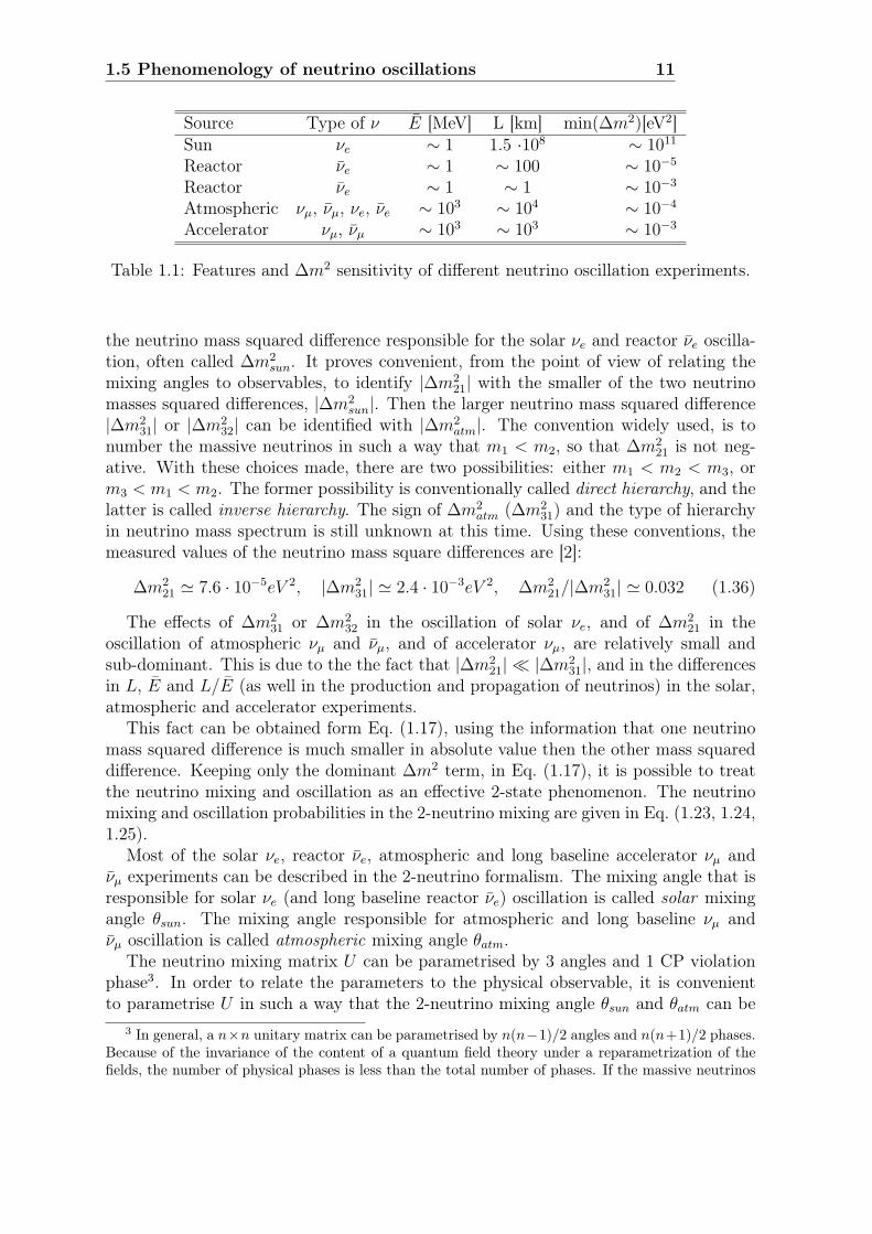
mixing matrix U . On the other hand, a given experiment searching for neutrino oscil-lation is characterised by the average energy of the neutrinos being studied, E, and bythe source-detector distance L. The requirement in Eq. (1.19) determines the minimalvalue of a generic neutrino mass squared difference to which the experiment is sensi-tive. Because of the interference nature of neutrino oscillations, oscillation experimentscan probe, in general, rather small values of ∆m2. Values of min(∆m2) characterisingqualitatively the sensitivity of different experiments are given in Table 1.1.
In the case of 3-neutrino mixing, there are only two independent neutrino massessquared differences, say ∆m2
21 and ∆m231. The numbering of massive neutrinos νi is
conventional. It follows from neutrino oscillation experiments that one of the two inde-pendent neutrino mass squared differences is much smaller in absolute value than thesecond one. In particular, the neutrino mass squared difference observed in the oscilla-tion atmospheric νµ and νµ, often called ∆m2
atm, is much larger in absolute value than
2except for the LSND result [47] , that has not been confirmed by MiniBOONE [48]
1.5 Phenomenology of neutrino oscillations 11
Source Type of ν E [MeV] L [km] min(∆m2)[eV2]Sun νe ∼ 1 1.5 ·108 ∼ 1011
Reactor νe ∼ 1 ∼ 100 ∼ 10−5
Reactor νe ∼ 1 ∼ 1 ∼ 10−3
Atmospheric νµ, νµ, νe, νe ∼ 103 ∼ 104 ∼ 10−4
Accelerator νµ, νµ ∼ 103 ∼ 103 ∼ 10−3
Table 1.1: Features and ∆m2 sensitivity of different neutrino oscillation experiments.
the neutrino mass squared difference responsible for the solar νe and reactor νe oscilla-tion, often called ∆m2
sun. It proves convenient, from the point of view of relating themixing angles to observables, to identify |∆m2
21| with the smaller of the two neutrinomasses squared differences, |∆m2
sun|. Then the larger neutrino mass squared difference|∆m2
31| or |∆m232| can be identified with |∆m2
atm|. The convention widely used, is tonumber the massive neutrinos in such a way that m1 < m2, so that ∆m2
21 is not neg-ative. With these choices made, there are two possibilities: either m1 < m2 < m3, orm3 < m1 < m2. The former possibility is conventionally called direct hierarchy, and thelatter is called inverse hierarchy. The sign of ∆m2
atm (∆m231) and the type of hierarchy
in neutrino mass spectrum is still unknown at this time. Using these conventions, themeasured values of the neutrino mass square differences are [2]:
∆m221 ' 7.6 · 10−5eV 2, |∆m2
31| ' 2.4 · 10−3eV 2, ∆m221/|∆m2
31| ' 0.032 (1.36)
The effects of ∆m231 or ∆m2
32 in the oscillation of solar νe, and of ∆m221 in the
oscillation of atmospheric νµ and νµ, and of accelerator νµ, are relatively small andsub-dominant. This is due to the the fact that |∆m2
21| � |∆m231|, and in the differences
in L, E and L/E (as well in the production and propagation of neutrinos) in the solar,atmospheric and accelerator experiments.
This fact can be obtained form Eq. (1.17), using the information that one neutrinomass squared difference is much smaller in absolute value then the other mass squareddifference. Keeping only the dominant ∆m2 term, in Eq. (1.17), it is possible to treatthe neutrino mixing and oscillation as an effective 2-state phenomenon. The neutrinomixing and oscillation probabilities in the 2-neutrino mixing are given in Eq. (1.23, 1.24,1.25).
Most of the solar νe, reactor νe, atmospheric and long baseline accelerator νµ andνµ experiments can be described in the 2-neutrino formalism. The mixing angle that isresponsible for solar νe (and long baseline reactor νe) oscillation is called solar mixingangle θsun. The mixing angle responsible for atmospheric and long baseline νµ andνµ oscillation is called atmospheric mixing angle θatm.
The neutrino mixing matrix U can be parametrised by 3 angles and 1 CP violationphase3. In order to relate the parameters to the physical observable, it is convenientto parametrise U in such a way that the 2-neutrino mixing angle θsun and θatm can be
3 In general, a n×n unitary matrix can be parametrised by n(n−1)/2 angles and n(n+1)/2 phases.Because of the invariance of the content of a quantum field theory under a reparametrization of thefields, the number of physical phases is less than the total number of phases. If the massive neutrinos

12 Neutrino oscillations
identified as 2 of the 3 mixing angles. The usual parametrisation of the neutrino mixingmatrix U is:
U =
c12c13 s12c13 s13e−iδ
−s12c23 − c12s23s13eiδ c12c23 − s12s23s12e
iδ s23c13
s12s23 − c12c23s13eiδ −c12s23 − s12c23s13e
iδ c23c13
(1.37)
where cij = cos θij, sij = sin θij, the angles θij = [0, π/2], δ = [0, 2π] is the Dirac CPviolation phase.
Short baseline reactor νe experiments (Palo Verde [50], CHOOZ [51], Double Chooz [32]),and long baseline accelerator νµ experiments (T2K [38], MINOS [36]), have shown that|Ue3|2 = | sin θ13|2 � 1. Because of this, one can identify θ12 as θsun and θ23 as θatm. Thesolar neutrino data have shown that ∆m2
21 cos 2θ12 > 0 (Sec. 2.4). In the conventionemployed, this means that cos 2θ12 > 0.
Supposing that in a given experiment |∆m231|L/(2E) ≥ 1, and ∆m2
21L/(2E) � 1.This is the case for the oscillations of reactor νe on a distance L ∼ 1 km (CHOOZ, DoubleChooz, Daya Bay [52], Reno [53] experiments), for the oscillation of the acceleratorνµ with distance L ∼ 103 km (K2K, T2K, MINOS, OPERA experiments). Under thisconditions, keeping only the oscillating terms involving ∆m2
31, the oscillation probabilityin Eq. (1.17) becomes:
P (να → νβ) ' P (να → νβ) ' δαβ − 2|Uα3|2(δαβ − |Uβ3|2
)(1− cos
∆m231
2EL
)(1.38)
The survival probability for oscillation of reactor νe on a distance L ∼ 1 km, is givenby Eq. 1.38 choosing α = β = e:
P (νe → νe) = P (νe → νe) ' 1− 2|Ue3|2(1− |Ue3|2
)(1− cos
∆m231
2EL
)(1.39)
The probability for oscillation of accelerator νµ into νe (or vice-versa) is given Eq. 1.38choosing α = µ, β = e:
P (νµ → νe) ' 2|Uµ3|2|Ue3|2(
1− cos∆m2
31
2EL
)(1.40)
=|Uµ3|2
1− |Ue3|2P 2ν
(|Ue3|2,m2
31
). (1.41)
Here P 2ν (|Ue3|2,m231) is the probability of the 2 neutrino transition νe → (s23νµ+c23ντ )
due to ∆m231 and a mixing with angle θ13, where,
sin2 θ13 = |Ue3|2, s223 = sin2 θ23 ≡
|Uµ3|2
1− |Ue3|2, c2
23 ≡ cos2 θ23 =|Uτ3|
1− |Ue3|2(1.42)
are Dirac particles, only (n− 1)(n− 2)/2 phases are physical and can be responsible for CP violationin the lepton sector. In the case the massive neutrinos νi are Majorana particles, i.e. particles thatcoincide with his own antiparticles, 2 additional physical CP violation phases, called Majorana phases,are present in U . However, Majorana phases have no effects in the neutrino oscillation phenomena andwill not mentioned further.

1.6 Conclusions and outlook 13
In certain cases the dimensions of the neutrino source, ∆L, are not negligible incomparison with the oscillation length. Similarly, when analysing neutrino oscillationdata one has to include the energy resolution of the detector, ∆E, in the analysis. Ascan be shown [54], if ∆L � E/∆m2, and/or L∆m2∆E/E2 � 1, the oscillating termsin the neutrino oscillation probabilities will be averaged out. This is the case for Solarneutrino oscillations in vacuum. In this case (as well as in the case of sufficiently largeseparation of the νi and νj neutrino wave packets at the detection point) the interferenceterms in the oscillation probability (or survival probability) will be negligibly small andthe neutrino flavour conversion will be determined by the average probabilities:
P (να → νβ) '∑i
|Uβi|2|Uαi|2 . (1.43)
This is the 3-neutrino mixing analog of Eq. 1.26.Suppose next that in the case of 3-neutrino mixing, ∆m2
21L/2E ∼ 1, while at the sametime |∆m31(32)|2L/2E � 1 and the oscillations due to ∆m2
31 and ∆m232 are averaged out
due to integration over the region of neutrino production, the energy resolution function,etc. This is the case for the oscillations of reactor νe observed by the KamLANDexperiment [31]. In this case we get for the νe and νe survival probabilities:
P (νe → νe) ' |Ue3|4 +(1− |Ue3|2
)2P 2ν(νe → νe) , (1.44)
P 2ν(νe → νe) = P 2ν(νe → νe) = 1− sin2 2θ12 sin2
(∆m2L
4E
)(1.45)
being the νe and νe survival probability in the case of 2-neutrino oscillation driven bythe angle θ12 and ∆m2
21, with θ12 determined by
cos2 θ12 =|Ue1|2
1− |Ue3|2, sin2 θ12 =
|Ue2|2
1− |Ue3|2. (1.46)
The existing neutrino oscillation data allow us to determine the parameters whichdrive the solar neutrino and the dominant atmospheric neutrino oscillations with arelatively good precision, and to obtain rather stringent limits on the mixing angle θ13.A comprehensive review on the solar, atmospheric, reactor, and accelerator neutrinooscillation experiments and their impact on the determination of θ12, θ23, θ13, ∆m2
21,and ∆m2
31 can be found on [2]. The relevant solar neutrino measurements and theirimpact on the determination of θ12 and ∆m2
21 are discussed extensively in Sec. 2.
1.6 Conclusions and outlookAfter the spectacular experimental progress made in the studies of neutrino oscillations,further understanding of the pattern of neutrino masses and neutrino mixing, of theyorigins and the status of the CP symmetry in the lepton sector requires an extensiveand challenging program of research. One of the targets of such a research programinclude the high precision measurement of the oscillation parameters that drive thesolar neutrino oscillations and test the MSW effect with neutrinos of different energies.Solar neutrinos are sensitive probe for pursuing this program.

Chapter 2
Solar neutrino observations
2.1 Introduction
Both the first evidence and the first discoveries of neutrino flavor transformation havecome from experiments which detected neutrinos from the Sun [55, 22, 23]. This dis-covery was remarkable, not only because it was unexpected, but because it was madeinitially by experiments designed to different physics. Ray Davis’s solar neutrino exper-iment [56] was created to study astrophysics, not the particle physics of neutrinos.
Observation of solar neutrinos directly addresses the theory of stellar structure andevolution, which is the basis of the standard solar models (SSMs). Neutrinos are indeedthe only particles which can travel undisturbed from the solar core to us, providing de-tails about the inner workings of the Sun. The Sun as a well-defined neutrino source alsoprovides extremely important opportunities to investigate nontrivial neutrino propertiessuch as nonzero mass, flavor mixing, neutrino oscillations, and MSW effect because ofthe wide range of matter density and the great distance from the Sun to the Earth. Thesolar neutrino flux is energetically broadband, free of flavor backgrounds, and passesthrough quantities of matter obviously unavailable to terrestrial experiments.
The chapter is organised as follows. In Section 2.2 I describe the Solar StandardModel. In Section 2.3, the solar metallicity problem is presented. Section 2.4 reports onthe pp fusion chain and the CNO cycle which fuel the Sun and produce solar neutrinos.In Section 2.5 I describe the propagation of solar neutrinos in the Sun, with emphasison the MSW effect. In Section 2.6 I review the experiments which have detected solarneutrinos, describing the detection method and their result. The discovery of solar neu-trino oscillations, as well with the current understanding of the MSW-LMA oscillationscenario is discussed in Section 2.7.
2.2 The Standard Solar Model
The stars are powered by nuclear fusion reactions. Two distinct processes, the mainpp fusion chain and the sub-dominant CNO cycle, are expected to fuel the Sun andproduce solar neutrinos with different energy spectra and fluxes (see Sec. 2.4 and [6]).

16 Solar neutrino observations
The combined effect of these reactions is written as
4p→ 4He + 2e+ + 2νe . (2.1)
Positrons annihilate with electrons. The overall reaction releases about 26.7 MeV intokinetic energy of the final particles, including neutrinos [6]. Each conversion of fourproton into an 4He nucleus is known as a termination of the chain of energy generatingreactions that accomplishes the nuclear fusion. The thermal energy that is suppliedby nuclear fusion ultimately emerges from the surface of the Sun as sunlight. Energyis transported in the deep solar interior mainly by photons, which means that theopacity of matter to radiation is important. The pressure that supports the Sun isprovided largely by the thermal motions of the electrons and ions. Some of the principalassumptions used in constructing standard solar models are [6]:
• Hydrostatic equilibrium: the Sun is assumed to be in hydrostatic equilibrium,that is, the radiative and particle pressures of the model exactly balances gravity.Observationally, this is known to be an excellent approximation since a gross de-parture from hydrostatic equilibrium would cause the Sun to collapse (or expand)in a free-fall time of less than a hour.
• Energy transport by photons or by convective motions: in the deep interior, whereneutrinos are produced, the energy transport is primarily by photon diffusion; thecalculated radiative opacity is a crucial ingredient in the construction of a modeland has been the subject of a number detailed studies.
• Energy generation by nuclear reactions: the primary energy source for radiatedphotons and neutrinos is nuclear fusion, although the small effects of gravitationalcontraction (or expansion) are also included.
• Abundance changes caused only by nuclear reactions: the initial solar interior ispresumed to have been chemically homogeneous. In regions of the model that arestable to matter convection, changes in the local abundances of individual isotopeoccur only by nuclear reactions.
A Standard Solar Model is the end product of a sequence of models. The calculationof a model begins with the description of a main sequence star that has a homogeneouscomposition. Hydrogen burns in the stellar core, supplying both the radiated lumi-nosity and the thermal pressure that supports the star against the gravity. Successivemodels are calculated by allowing for composition changes caused by nuclear reactions,as well as the mild evolution of other parameters, such as the surface luminosity andthe temperature distribution inside the star. The models that describe later times inan evolutionary sequence have inhomogeneous compositions.
A satisfactory solar model is a solution of the evolutionary equation that satisfiesboundary conditions in both space and time. Solar astrophysicists seek models with afixed mass M�, with a total luminosity L�, and with an outer radius R� at an elapsedtime of 4.6 ·109 years (the present age of the Sun, determined accurately from meteoriticages). The assumed initial values of chemical composition and entropy are iterated untilan accurate description is obtained of the Sun. The solution of the evolution equations

2.3 The Solar Metallicity Problem 17
determines the initial values for the mass fractions of hydrogen, helium, and heavyelements, the present distribution of physical variables inside the Sun, the spectrum ofacoustic oscillation frequencies observed on the surface of the Sun, and the neutrinofluxes [6].
The most elaborate SSM calculations have been developed by Bahcall and his col-laborators1, who define their SSM as the solar model which is constructed with the bestavailable physics and input data. Therefore, their SSM calculations have been rather fre-quently updated. SSM’s labelled as BS05(OP) [57], BSB06(GS) and BSB06(AGS) [58],BPS08(GS) and BPS08(AGS) [59], and BPS11(GS) and BPS11(AGSS) [60] representrecent model calculations.
Here, OP means that newly calculated radiative opacities from the Opacity Projectare used. The later models are also calculated with OP opacities. GS and AGS refer toold and new determinations of solar abundances of heavy elements. There are significantdifferences between the old, higher heavy element abundances (henceforth GS, [61]) andthe new, lower heavy element abundances (henceforth AGS, [62] and AGSS, [63]). Themodels with GS are consistent with helioseismological data, but the models with AGSand AGSS are not [64]. The measurement of the flux of the neutrinos resulting fromthe CNO cycle may help to resolve this Solar Metallicity Problem.
2.3 The Solar Metallicity ProblemThe solar heavy-element abundance2, Z, is one of the important inputs in solar modelcalculations. The heavy-element abundance affects solar structure by affecting radiativeopacities [6]. The abundance of oxygen, carbon, and nitrogen also affect the energygeneration rates through the CNO cycle (see Sec. 2.4 and [6]). The effect of Z onopacities changes the boundary between the radioactive and convective zones, as wellas the structure of radiative region; the effect of Z on energy generation rates can changethe structure of the core [64]. Solar Z is not only important in modelling the Sun, itis also important for other fields of astrophysics. The heavy-element abundance of theSun is usually used as a reference in studies of the metallicity of stars, the chemicalevolution of galaxies; thus, an accurate knowledge of solar metallicity is important.
Till the early part of last decade, the solar abundance compilation of Grevesse andSauval (GS98, [61]), with the ratio between heavy-element and hydrogen abundanceZ/X = 0.023, was used. In a series of papers Allende-Prieto [65, 66] and Asplund andothers [67, 68] have revised the spectroscopic determinations of the solar photosphericcomposition using sophisticated 3D stellar atmospheric models. These models wereobtained by 3D radiation-hydrodynamic simulations of the near-surface layers of theSun. Their results indicated that the solar carbon, nitrogen, and oxygen abundancesare lower by about 35% to 45% than those listed by GS98. The revision of the oxygenabundance led to a comparable change in the abundances of neon and argon too, sincethese abundances are generally measured through the abundance ratio for Ne/O andAr/O. Additionally, Asplund [69] also determined a lower value (by about 10%) for
1 Bahcall passed away in 2005, but his program to improve SSM is still pursued by his collaborators2 in astrophysics, any element with atomic number greater than helium is labelled as heavy-element,
or metal

18 Solar neutrino observations
the photospheric abundance of silicon compared with the GS98 value. As a result, allthe elements for which abundances are obtained from meteoritic measurements haveseen their abundances reduced by a similar amount. These measurement have beensummarised by Asplund, Grevesse and Sauval (AGS05, [62]). The net result of thesechanges is that Z/X for the Sun is reduced to 0.0165 (or Z = 0.0122) in AGS05,about 28% lower than the previous value of GS98 Z/X ∼ 0.023. The most recentand complete revision by Asplund et al. (AGSS09, [63]) also shows a reduction in theabundances of the volatile CNO elements and Ne with respect to the older compilationof solar abundances of GS98.
The consequence of this reduction of the solar Z/X is that the structure of the solarmodels do not agree well with the helioseismically determined structure of the Sun anymore [64]. In particular, the relative sound-speed and density in solar models with theAGS05 abundances disagrees with the experimental data a lot more than models withGS98 abundances. The main reason for the disagreement is the difference in the positionof the convection zone (CZ) base between the model and the Sun. The AGS05 modelhas its CZ base at 0.729R�, in contrast the CZ base of the Sun is at 0.713 ± 0.001R�[64]. Additionally, solar models with AGS05 abundances have lower helium abundances(Y ) than the Sun, Y = 0.230 rather than the helioseismically determined solar heliumabundance of Y = 0.2485± 0.0034 [64]. The GS98 solar model by contrast has CZ baseat 0.715R� and helium abundance of Y = 0.243, much closer to the real solar values.
A competitive source of information about the solar core that may solve the SolarMetallicity Problem are the neutrino emitted in the CNO cycle. SSMs with high heavy-element abundance, such as BPS08(GS) [59], predict a total CNO neutrino flux of(5.4 ± 0.8) × 108 cm−2 s−1, while SSMs with low heavy-element abundance, such asAGSS09, predict a 30% lower CNO flux of (3.8+0.6
−0.5) × 108 cm−2 s−1 [60]. One of theresult of this PhD thesis is the strongest constrain on the CNO neutrino flux up to date,which leads to the strongest test of the solar metallicity up to date (see Sec. 5.10).
2.4 Production of solar neutrinos
The solar neutrinos are produced by some of the fusion reactions in the pp chain orthe CNO cycle [6]. In both processes, the net effect is the fusion of four protons in a4He nucleus. About 600 million tons of hydrogen are burned every second to supplythe solar luminosity. The main nuclear burning mechanism in the Sun is the proton-proton chain (or pp chain). A sub dominant and still undetected process for the energygeneration in the Sun is the Carbon-Nitrogen-Oxygen cycle (or CNO cycle), in whichthe fusion of four protons into a 4He nucleus is achieved through reactions involvingcarbon, nitrogen and oxygen. The CNO cycle is supposed to be a dominant processfor massive stars (> 1.5, M�), in which the heavy-element abundance is high. TheSSM prediction for the fluxes from neutrino-producing reactions is given in Table 2.4.Fig. 2.1 shows the solar neutrino spectra calculated with the BS05(OP) model which issimilar to the BPS08(GS) model.
In the following subsections, the reactions of pp chain and CNO cycle, as well withthe neutrinos created in such processes, are described in detail.

2.4 Production of solar neutrinos 19
Figure 2.1: The solar neutrino spectrum predicted by the BS05(OP) standard solarmodel [57]. The neutrino fluxes are given in units of cm−2s−1MeV−1 for continuousspectra and cm−2s−1 for line spectra. The numbers associated with the neutrino sourcesshow theoretical errors of the fluxes.
2.4.1 The pp chain
The pp chain has three branches, named pp - I, pp - II and pp - III. The net process ineach termination of the pp chain is:
4p → 4He + 2e+ + 2νe, (2.2)
with Q-value3 Q=24.7 MeV. In some cases, the process is 4p + e− → 4He + e+ + 2νe.The positrons annihilate with free electrons in the solar plasma (with γ-rays with totalenergy of 2mec
2 = 1.02 MeV emitted for each annihilation). The total energy gain ineach termination of the pp chain is ∼ 26.7 MeV, on which, on average, only a smallamount is carried away by neutrinos. The energy of the neutrinos emitted in the ppchain depends on its particular termination.
The first step of each branch is one of this weak interaction processes (the energyavailable to the final states body, the Q-value, is written in brackets):
p+ p → 2H + e+ + νe (0.42MeV) (2.3)3the Q-value is defined as the difference between the initial state total mass and final state total
mass, and it is equal, in natural units, to the total kinetic energy available to the final state particles
20 Solar neutrino observations
Reaction Abbr. Energy (MeV) GS98 Flux AGSS09 Flux exppp→ 2H e+ ν pp 0 - 0.42 5.98 (1 ± 0.006) 6.03 (1 ± 0.006) 1010
pe−p→ 2H ν pep 1.44 1.44 (1 ± 0.012) 1.47 (1 ± 0.012) 108
3He p→ 4He e+ ν hep 0 - 19.79 8.04 (1 ± 0.30) 8.31 (1 ± 0.30) 103
7Be e− → 7Li ν 7Be 0.862 (0.383) 5.00 (1 ± 0.07) 4.56 (1 ± 0.07) 109
8B→ 8Be e+ ν 8B 0 - 17.98 5.58 (1 ± 0.14) 4.59 (1 ± 0.14) 106
13N→ 13C e+ ν 13N 0 - 1.19 2.96 (1 ± 0.14) 2.17 (1 ± 0.14) 108
15O→ 15C e+ ν 15O 0 - 1.73 2.23 (1 ± 0.15) 1.56 (1 ± 0.15) 108
17F→ 17C e+ ν 13F 0 - 1.74 5.52 (1 ± 0.17) 3.40 (1 ± 0.16) 106
CNO cycle CNO 0 - 1.74 5.24 (1 ± 0.84) 3.76 (1 ± 0.60) 108
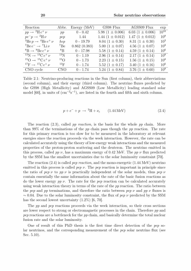
Table 2.1: Neutrino-producing reactions in the Sun (first column), their abbreviations(second column), and their energy (third column). The neutrino fluxes predicted bythe GS98 (High Metallicity) and AGSS09 (Low Metallicity) leading standard solarmodel [60], in units of (cm−2s−1), are listed in the fourth and fifth and sixth column.
p+ e− + p → 2H + νe (1.44MeV) (2.4)
The reaction (2.3), called pp reaction, is the basis for the whole pp chain. Morethan 99% of the terminations of the pp chain pass though the pp reaction. The ratefor this primary reaction is too slow for to be measured in the laboratory at relevantenergies since the reaction proceeds via the week interaction. However, the rate can becalculated accurately using the theory of low-energy weak interactions and the measuredproperties of the proton-proton scattering and the deuteron. The neutrino emitted inthis process, called pp ν, has a maximum energy of 0.42 MeV. The pp ν flux predictedby the SSM has the smallest uncertainties due to the solar luminosity constraint [70].
The reaction (2.4) is called pep reaction, and the mono-energetic (1.44 MeV) neutrinoemitted in this process is called pep ν. The pep reaction is important in principle sincethe ratio of pep ν to pp ν is practically independent of the solar models, thus pep νcontain essentially the same information about the rate of the basic fusion reactions asdo the lower energy pp ν. The rate for the pep reaction can be calculated accuratelyusing weak interaction theory in terms of the rate of the pp reaction. The ratio betweenthe pep and pp terminations, and therefore the ratio between pep ν and pp ν fluxes is∼ 0.04. Due to the solar luminosity constraint, the flux of pep ν predicted by the SSMhas the second lowest uncertainty (1.2%) [6, 70].
The pp and pep reactions proceeds via the week interaction, so their cross sectionsare lower respect to strong or electromagnetic processes in the chain. Therefore pp andpep reactions are a bottleneck for the pp chain, and basically determine the total nuclearfusion rate and the solar luminosity.
One of result of this PhD thesis is the first time direct detection of the pep so-lar neutrinos, and the corresponding measurement of the pep solar neutrino flux (seeSec. 5.10).

2.4 Production of solar neutrinos 21
The pp− I branch
The pp− I branch of the pp chain proceeds through the reaction:
p+ 2H → 3He + γ (5.49MeV) (2.5)
The 3He nucleus can interact in three different ways:
3He + 3He → 4He + 2p (12.86MeV) (2.6)
3He + 4He → 7Be + γ (1.59MeV) (2.7)
3He + p → 4He + e+ + νe (19.79MeV) (2.8)
The cross sections of the reactions Eq. 2.5, Eq. 2.6, and Eq. 2.7 have been measuredby the LUNA collaboration [71, 72, 73, 74, 75]. The reaction (2.6) is the dominanttermination in the Sun, because of the abundance of 3He; SSMs predict this reaction tocomplete ∼ 85% of pp chain terminations.
The reaction (2.8), called hep reaction is a weak interaction process which producesthe highest-energy solar neutrinos. The neutrinos from this reactions are extremelyrare, and have never been detected so far [76].
The reaction (2.7) leads to the two important neutrino-producing reactions involving7Be. The two terminations involving the 7Be nucleus are called pp− II and pp− III.
The pp− II branch
In the Sun, 7Be is almost always destroyed by electron capture, usually from free elec-trons in the solar plasma:
7Be + e− → 7Li + νe (0.862MeV) (2.9)
7Li + p → 4He + 4He (17.34MeV) (2.10)
The rate of the process (2.9) can be calculated accurately using weak interaction theory.The mono-energetic neutrino emitted in the electron capture of the 7Be is called 7Be ν.The 7Li nucleus can be generated in an excited state with energy 487 keV, with branchingfactor of 10%. Therefore, the energy of 7Be ν can be either 862 keV or 384 keV. Theflux of 7Be ν has been measured with a precision of 5% by the Borexino experiment[25, 77, 78].
22 Solar neutrino observations
The pp− III branch
The 7Be + p reaction occurs only rarely in the SSMs, in about 1 out of 5000 terminationsof the pp chain (the 7Be electronic capture reaction is about a thousand time moreprobable):
7Be + p → 8B + γ (0.14MeV) (2.11)
8B → 8Be + e+ + νe (17.98MeV) (2.12)8Be → 4He + 4He (0.14MeV) (2.13)
Nevertheless, this branch is of crucial importance since it leads to high energy 8B ν.8B νs have an extremely historical importance: they have been the first detected solarneutrinos in the Homestake experiment in the 60s [55, 14], and their detection withdifferent channel in SNO lead to first evidence of neutrino oscillation [22, 23, 79, 80].The first time detection of 8B νs with a 3 MeV threshold (kinetic energy of electronrecoil) has been performed in Borexino [81].
2.4.2 The CNO chain
In the set of reaction in the carbon-nitrogen-oxygen cycle (CNO cycle), the overallconversion of four protons to form an helium nucleus, two positrons, and two electronneutrinos is achieved with the aid of 12C, the most abundant heavy isotope in normalstellar condition:
12C + 4p → 12C +4 He + 2e+ + 2νe . (2.14)
The total energy release is the same as for the pp chain (26.7 MeV).The energy production in the CNO cycle only constitutes a small contribution to the
total luminosity in the Sun (of the order of ∼ 1% in the SSMs). The Coulomb barrierbetween a proton and carbon or nitrogen nuclei is much higher than the one betweentwo protons or helium nuclei, therefore the CNO cycle can only occur at temperaturemuch higher than the temperature needed for pp chain [6]. The CNO cycle is believedto be the dominant mechanism of energy production massive stars (> 1.5M�).
The CNO cycle have two sub-cycles: the CN cycle and the sub-dominant NO cycle.The NO cycle rate is about 2× 10⁻² the CN rate. The reactions in the CN cycle are:
12C + p → 13N + γ (1.94MeV) (2.15)13N → 13C + e+ + νe (1.19MeV) (2.16)
13C + p → 14N + γ (7.55MeV) (2.17)14N + p → 15O + γ (7.30MeV) (2.18)
15O → 15N + e+ + νe (1.73MeV) (2.19)15N + p → 16O∗ → 12C + 4He (4.97MeV) (2.20)
The half lifes of 13N and 15O are about some minutes. The α-decay of the excited 16O∗
has a higher branching ratio respect to its γ decay. The cross sections of the reactions
2.5 Propagation of solar neutrinos 23
Eq. 2.18 and Eq. 2.21, have been measured by the LUNA collaboration [82, 83, 84].The γ-decay of 16O∗ is the first process in the NO cycle:
15N + p → 16O + γ (12.13MeV) (2.21)16O + p → 17F + γ (0.60MeV) (2.22)
17F → 17O + e+ + νe (1.74MeV) (2.23)17O + p → 14N + 4He (2.24)
The neutrinos resulting from the CNO cycle are called CNO νs. The energy spectrumof the CNO νs is the sum of three continuous spectra with end point energies of 1.19MeV (13N), 1.73 MeV (15O), and 1.74 MeV (17F). The total predicted CNO νs flux isstrongly dependent on the inputs of the solar modelling, being 40% higher in the HighMetallicity (GS98) than in the Low Metallicity (AGSS09) solar model (see Sec. 2.3,Table 2.4). The detection of neutrinos resulting from the CNO cycle has importantimplications in astrophysics, as it would be the first direct evidence of the nuclearprocess that is believed to fuel massive stars (> 1.5M�). Furthermore, its measurementmay resolve the solar metallicity problem.
One of the results of this PhD thesis is the strongest constraint of the CNO solarneutrino flux to date (see Sec. 5.10).
2.5 Propagation of solar neutrinos
The solar νes undergo oscillations while they propagate from the central part of theSun, where they are produced, to the terrestrial detector. Because of the large range ofmatter density in the Sun, matter effects (see Sec. 1.4) have a significant role in the solarneutrino oscillations. The electron number density Ne changes considerably along theneutrino path in the Sun: it decreases monotonically from the value of ∼ 100 cm−3NA
in the centre of the Sun to 0 at the surface of the Sun. According to the contemporarysolar models, Ne decreases approximately exponentially in the radial direction towardsthe surface of the Sun:
Ne(t) = Ne(t0) exp(−t− t0
r0
), (2.25)
where (t − t0) ' d is the distance travelled by the neutrino in the Sun, Ne(t0) is theelectron number density at the point of νe production in the Sun, r0 is the scale-heightof the change of Ne(t) and one has [6, 58] r0 ∼ 0.1R�.
Consider the case of 2-neutrino mixing in matter, Eq. (1.31). If Ne changes with t (orequivalently with distance) along the neutrino trajectory, the matter-eigenstates, theirenergies, the mixing angle, and the oscillation length in the matter become, throughtheir dependence on Ne, also functions of t. The behaviour of the neutrino system canbe understood in term of a two-level system whose Hamiltonian depends on time. Therelevant cases for solar neutrinos, are that the electron number density at the point of asolar νe production in the Sun much bigger, or much smaller than the resonance density.
In the case Ne(t0) � N rese , θm(t0) ' π/2 and the state of the electron neutrino in
the initial moment of evolution of the system practically coincides with the heavier of

24 Solar neutrino observations
the two matter eigenstates:|νe〉 ' |νm2 (t0)〉 . (2.26)
When neutrinos propagate to the surface of the Sun they cross a layer of matter inwhich Ne = N res
e . Correspondingly, the evolution of the neutrino system can proceedbasically in two ways: either evolve adiabatically or jump.
In the adiabatic evolution, characterised by the negligible probability of the jump fromthe upper matter eigenstate to the lower matter eigenstate, the system can stay on thestate |νm2 (t)〉 up to the final moment ts, when the neutrino reaches the surface of theSun. At the surface of the Sun Ne(ts) = 0 and therefore θm(ts) = θ, |νm1,2(ts)〉 = |ν1,2〉.Thus, in this case the state describing the neutrino system at t0 will evolve continuouslyinto the state |ν2〉 at the surface of the Sun. The probabilities to find νe and νµ at thesurface of the Sun are then (Eq. (1.23)):
P (νe → νe; ts) ' |〈νe|ν2〉|2 = sin2 θ (2.27)P (νe → νµ; ts) ' |〈νµ|ν2〉|2 = cos2 θ . (2.28)
Under the assumption made, a νe → νµ conversion with P > 0.5 is possible.The other possibility is realised if in the resonance region the system jumps from
the upper matter eigenstate to the lower matter eigenstate and after that the systemcontinues to be in the state |νm1 (t)〉 until the neutrino reaches the surface of the Sun.
The value of the jump probability P ′ plays a crucial role in the solar neutrino oscil-lations. There exist a whole spectrum of possibilities since P ′ can have any value from0 to cos2 θ [85, 86]. In the literature, the transitions are called nonadiabatic if P ′ is nonnegligible. In order for the evolution to be adiabatic, Ne(t) should change sufficientlyslow along the neutrino path [87]. Numerical studies have shown [42] that solar neutri-nos can undergo both adiabatic and nonadiabatic transition, and the matter effect canbe substantial in the solar neutrino oscillations for 10−8eV2 < ∆m2
sun < 10−4eV2 and10−4 < sin2 2θsun < 1.0.
The evolution equations Eq. (1.28) for the neutrino state in matter can be solvedexactly for Ne changing exponentially, as in Eq. (2.25), along the neutrino path in theSun [85, 88]. On the basis of the exact solution it was possible to derive a completeand accurate analytic description of the matter-enhanced transitions of solar neutrinosin the Sun for any values of ∆m2
sun and θsun [41, 42, 85, 86].The survival probability for a νe produced in the central part of the Sun on its way
to the surface of the Sun is given by
P 2ν� (νe → νe) =
1
2+(
1
2− P ′
)cos 2θm cos 2θ , (2.29)
where θm is the mixing angle in matter at the point of νe production and the jumpprobability P ′ in terms of ∆m2, sin2 θ, the neutrino energy E, and r0 (Eq. 2.25) is givenin [85]. This equation is only valid valid for the convention ∆m2
21 > 0 but for both signsof cos 2θ12.
The current solar neutrino and KamLAND data suggest that ∆m221' 7.6 · 10−5 eV2.
For ∆m221> 10−7 eV2 , the averaging over the region of neutrino production in the Sun
renders negligible all interference terms which appear in Eq. (1.25). Thus, the survival

2.5 Propagation of solar neutrinos 25
probability of a νe while it travels from the central part of the Sun to the surface of theEarth is effectively equal to the survival probability of the νe while it propagates fromthe central part to the surface of the Sun (Eq. (2.29)).
If the solar νe transitions are adiabatic, P ′ ' 0 and cos 2θm ' −1, the survivalprobability given by Eq. (2.29) becomes [42]
P 2ν� (νe → νe) '
1
2− 1
2cos 2θ = sin2 θ . (2.30)
The solar neutrino and KamLand data4 suggest sin2 2θ12 ∼ 0.8. For such mixing an-gle, the adiabatic transitions are realised if E/∆m2 lies approximately in the range(2 · 104 − 3 · 107) MeV/eV2 [86]. This result is relevant for the interpretation of thesolar 8B ν data, detected by Super-Kamiokande, SNO and Borexino. The measuredsurvival probability for 8B ν of energy E > 5MeV is P (νe → νe) ' 0.3. A solar νesurvival probability < 1/2 is not allowed by oscillations in vacuum (Eq. (1.26)), there-fore the data evidence that 8B ν oscillations are driven by matter effects. The survivalprobability given in Eq. (2.30) is indeed either bigger or smaller than 1/2 depending onthe sign of cos 2θ. Thus, the possibility of cos 2θ < 0 is ruled out by the data. Giventhe convention ∆m2
21 > 0 adopted, the data imply that ∆m221 cos 2θ12. The solar νe
oscillation undergoing for E > 5 MeV are often called Matter Enhanced.If E/∆m2 is sufficiently small so that Ne(t0) � N res
e , we have P ′ ' 0, θm ' 0 andthe oscillations take place in the Sun as in vacuum [42]:
P 2ν� (νe → νe) ' 1− sin2 2θ , (2.31)
which is the average two-neutrino survival probability in vacuum (Eq. (1.26)). Thisexpression describes with good precision the transitions of the solar pp ν. The solar νeoscillation undergoing in the energy region of pp νs are often called Vacuum Dominated.
The energy region between the vacuum dominated and matter enhanced solar νeoscillation regime is called Transition Region. The current framework of solar neutrinooscillation, MSW-LMA, predicts a smooth transition of the νe survival probability be-tween the two regions, resulting in an energy dependent νe survival probability Pee.The solar νe survival probability as a function of the energy and the corresponding Peemeasurement from solar neutrinos are shown in Fig. 5.25.
The solar νe survival probability in the case of 3-neutrino mixing takes a simple formfor |∆m2
31| � |∆m221|. Indeed, for the energies of solar neutrinos E < 10MeV , N res
e
corresponding to ∆m231 satisfies Ne(t0) << N res
e31 . As a consequence, the oscillations dueto ∆m2
31 proceed as in vacuum. The averaging over the region of νe production in theSun strongly suppress the oscillations due to ∆m2
31. The 3-neutrino solar νe survivalprobability is then [89, 90]:
P 3ν� (νe → νe) ' sin4 θ13 + cos4 θ13P
2ν� (∆m2
21, θ12;Ne cos2 θ13) , (2.32)
where P 2ν� (∆m2
21, θ12;Ne cos2 θ13) is given by Eq. (2.29) in which ∆m2 = ∆m221, θ = θ12
and the solar e− number density Ne is replaced by Ne cos2 θ13.4 in the literature, the configuration of ∆m2
21 and θ12 suggested by the solar neutrino and KamLanddata is often called Large Mixing Angle (LMA). Recently, the Borexino collaboration have validatedthe LMA configuration with solar νe only, i.e. without using KamLand νe data and the assumption ofCPT invariance [26]
26 Solar neutrino observations
2.6 Detection of solar neutrinosSo far, solar neutrinos have been observed by chlorine (Homestake) and gallium (SAGE,GALLEX and GNO) radiochemical detectors and water Cherenkov detectors using lightwater (Kamiokande and Super-Kamiokande) and heavy water (SNO). Recently, lowenergy solar neutrinos have been successfully observed by the liquid scintillator detectorBorexino.
A pioneering solar neutrino experiment by Davis and collaborators at Homestakeusing the 37Cl −37 Ar method proposed by Pontecorvo [91] started in the late 1960’s.This experiment exploited νe absorption on 37Cl nuclei followed by the produced 37Ardecay through orbital e− capture,
νe + 37Cl→ 37Ar + e− . (2.33)
The neutrino energy threshold is 814 keV. The 37Ar nuclei produced are radioactive,with a half life (τ1/2) of 34.8 days. After an exposure of the detector for two or threetimes τ1/2, the reaction products were chemically extracted and introduced into a lowbackground proportional counter, where they were counted for a sufficient long period todetermine the exponentially decaying signal and a constant background. Solar modelcalculations predict that the dominant contribution in the chlorine experiment camefrom 8B neutrinos, but 7Be, pep and CNO neutrinos also contributed.
From the very beginning of the solar neutrino observations [55], it was recognisedthat the observed flux was significantly smaller than the SSM predictions, providednothing happens to the νe after the creation in the solar interior. This deficit has beencalled the Solar Neutrino problem.
Gallium experiments (GALLEX and GNO at Gran Sasso in Italy and SAGE atBaksan in Russia) exploit the reaction
νe + 71Ga→ 71Ge + e− . (2.34)
The neutrino energy threshold is 233 keV. The dominant contribution is given by themost abundant pp neutrinos. However, the solar model calculations predict almost halfof the capture rare in gallium due to other solar neutrinos. GALLEX presented thefirst evidence of pp ν observation in 1992 [16]. The GALLEX Collaboration finishedobservations in early 1977 [17]. Since April, 1998, the GNO (Gallium Neutrino Obser-vatory) collaboration continued the observation until April 2003. The GNO and GNO+ GALLEX joint analysis results are presented in [18]. SAGE initially reported verylow flux [92], but later observed similar flux to that of GALLEX. The latest SAGEresults are published in [19]. The SAGE experiment continues to collect data.
In 1987, the Kamiokande experiment in Japan succeeded in real-time solar neutrinoobservations, exploiting νe scattering,
νx + e− → νx + e− , (2.35)
in a large water-Cherenkov detector. This experiment takes advantage of the direc-tional correlation between the incoming neutrino and the recoil electron. This featuregreatly helps the clear separation of the solar-neutrino signal from the background. The
2.6 Detection of solar neutrinos 27
Kamiokande result gave the first direct evidence that neutrinos come from the directionof the Sun [93]. Later, the high-statistics Super-Kamiokande experiment [94, 95, 21]with a 50-kton water Cherenkov detector replaced the Kamiokande experiment. Due tohigh thresholds (7 MeV in Kamiokande and 5 MeV at present in Super-Kamiokande)the experiments observe pure 8B solar neutrinos. The ν−e elastic scattering is sensitiveto all active neutrinos x = e, µ, τ . However, the sensitivity to νµ and ντ is much smallerthan the sensitivity to νe, being σ(νµ,τ − e) ∼ 0.16σ(νe − e).
In 1999, a new real time solar neutrino experiment, SNO (Sudbury Neutrino Obser-vatory), in Canada started observation. This experiment used 100 tons of ultra-pureheavy water (D2O) contained in a spherical acrylic vessel, surrounded by an ultra-pureH2O shield. SNO measured 8B solar neutrinos via the charged-current (CC) and neutralcurrent (NC) reactions
νe + d→ e− + p + p (CC) , (2.36)
andνx + d→ νx + p + n (NC) , (2.37)
as well as νe elastic scattering on electron (Eq. (2.35)). The CC reaction is sensitive onlyto νe, while the NC reaction is sensitive to all active neutrinos. This is a key feature tosolve the solar neutrino problem. If it is caused by flavour transition such as neutrinooscillations, the solar neutrino fluxes measured by CC and NC reactions would show asignificant difference. The neutrino energy threshold of the CC reaction is 1.4 MeV andthe e− energy is strongly correlated with the νe energy. Thus, the CC reaction providesan accurate measure of the shape of the 8B ν energy spectrum. The contributions fromCC reaction and νe scattering can be distinguished by using different cosφ distributions,where φ is the angle of the e− momentum with respect to the Sun-Earth axis. While theνe elastic scattering events have a strong forward peak, CC events have an approximateangular distribution of 1− 1/3 cosφ. The neutrino energy threshold of the NC reactionis 2.2 MeV. In the pure D2O [22, 23], the signal of the NC reaction was neutron capturein deuterium, producing a 6.25 MeV γ-ray. In this case, the capture efficiency waslow and the deposited energy was close to the detection threshold of 5 MeV. In orderto enhance both the capture efficiency and the total γ-ray energy (8.6 MeV), 2 tonsof NaCl were added to the heavy water in the second phase of the experiment [79].Subsequently NaCl was removed and an array of 3He neutron counters were installedfor the third phase measurement [80]. These neutrons counters provided independentNC measurement with different systematics from that of the second phase, and thusstrengthened the reliability of the NC measurement.
Borexino at Gran Sasso in Italy started solar neutrino observation in May 2007.Borexino detects solar neutrinos via νe scattering in 300 tons of ultra-pure liquid scin-tillator [96]. The flux of the mono-energetic 862 keV 7Be solar neutrinos has beendirectly observed for the first time [78, 77]. Recently, a precise measurement of the7Be ν at 5% precision has been published by the Borexino collaboration [25]. Borexinohas also measured solar 8B ν with an analysis threshold as low as 3 MeV (effectiveelectron kinetic energy) [81]. The first time detection of pep and the strongest limits sofar on CNO solar neutrinos in Borexino are the results of this PhD thesis. More detailson the Borexino detector and the pep and CNO solar neutrinos analysis will be given
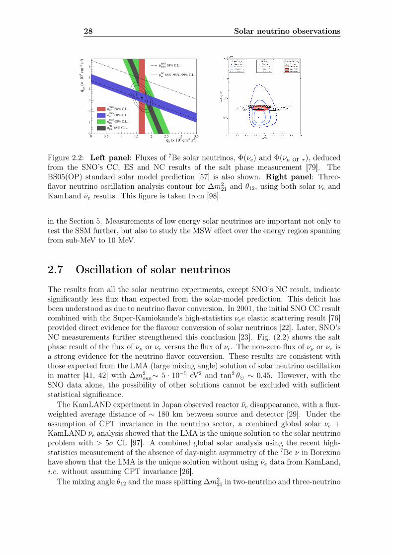
28 Solar neutrino observations
)-1 s-2 cm6 10× (e!0 0.5 1 1.5 2 2.5 3 3.5
)-1 s-2
cm
6 1
0× ( "
µ!
0
1
2
3
4
5
6
68% C.L.CCSNO!
68% C.L.NCSNO!
68% C.L.ESSNO!
68% C.L.ESSK!
68% C.L.SSMBS05!
68%, 95%, 99% C.L."µNC!
Figure 2.2: Left panel: Fluxes of 7Be solar neutrinos, Φ(νe) and Φ(νµ or τ ), deducedfrom the SNO’s CC, ES and NC results of the salt phase measurement [79]. TheBS05(OP) standard solar model prediction [57] is also shown. Right panel: Three-flavor neutrino oscillation analysis contour for ∆m2
21 and θ12, using both solar νe andKamLand νe results. This figure is taken from [98].
in the Section 5. Measurements of low energy solar neutrinos are important not only totest the SSM further, but also to study the MSW effect over the energy region spanningfrom sub-MeV to 10 MeV.
2.7 Oscillation of solar neutrinos
The results from all the solar neutrino experiments, except SNO’s NC result, indicatesignificantly less flux than expected from the solar-model prediction. This deficit hasbeen understood as due to neutrino flavor conversion. In 2001, the initial SNO CC resultcombined with the Super-Kamiokande’s high-statistics νee elastic scattering result [76]provided direct evidence for the flavour conversion of solar neutrinos [22]. Later, SNO’sNC measurements further strengthened this conclusion [23]. Fig. (2.2) shows the saltphase result of the flux of νµ or ντ versus the flux of νe. The non-zero flux of νµ or ντ isa strong evidence for the neutrino flavor conversion. These results are consistent withthose expected from the LMA (large mixing angle) solution of solar neutrino oscillationin matter [41, 42] with ∆m2
sun∼ 5 · 10−5 eV2 and tan2 θ� ∼ 0.45. However, with theSNO data alone, the possibility of other solutions cannot be excluded with sufficientstatistical significance.
The KamLAND experiment in Japan observed reactor νe disappearance, with a flux-weighted average distance of ∼ 180 km between source and detector [29]. Under theassumption of CPT invariance in the neutrino sector, a combined global solar νe +KamLAND νe analysis showed that the LMA is the unique solution to the solar neutrinoproblem with > 5σ CL [97]. A combined global solar analysis using the recent high-statistics measurement of the absence of day-night asymmetry of the 7Be ν in Borexinohave shown that the LMA is the unique solution without using νe data from KamLand,i.e. without assuming CPT invariance [26].
The mixing angle θ12 and the mass splitting ∆m221 in two-neutrino and three-neutrino
2.8 Conclusions and outlook 29
oscillation framework are obtained from a global analysis including all the solar neutrino(SNO, Super-Kamiokande, chlorine, gallium, and Borexino) and the KamLAND data.One recent update can be found in [98]. The allowed parameter regions obtained from[98] are shown in Fig. 2.2. The best fit parameters obtained from the global solar +KamLAND analysis are ∆m2
21 = 7.46+0.20−0.19 ·10−5eV2 and tan2 θ12 = 0.427+0.027
−0.024, and thosefrom the global solar analysis are ∆m2
21 = 5.13+1.29−0.96 · 10−5eV2 and tan2 θ12 = 0.427+0.028
−0.028.
2.8 Conclusions and outlookThe MSW-LMA scenario is our current understanding of solar neutrino oscillations.This scenario yields to an electron neutrino survival probability Pee that depends onthe neutrino energy. The energy dependence Pee(E) is predicted with high accuracy inthe context of MSW-LMA oscillations and the Solar Standard Model (see Sec. 2.4).
Before the Borexino measurements, precision tests to the Pee, thus to MSW-LMAoscillations, were only available with high energy 8B solar neutrinos, in the matter-enhanced energy region. Spectral measurements or high precision measurements of subMeV solar neutrinos, in the vacuum-dominated energy region, were not available. BeforeBorexino, the detection of sub MeV solar neutrinos were only performed with galliumand chlorine radiochemical experiments, which are only sensitive the total neutrino fluxabove the reaction threshold. Thus, the predictions of the MSW-LMA scenario in thevacuum-dominated and transition region of the Pee were poorly tested.
Moreover, reactor neutrino experiments are only sensitive to νe, therefore one hasto assume that νe oscillations behave in the same way of νe oscillations (i.e. CPTinvariance holds in the neutrino sector) in order to combine νe and νe oscillation datato determine the oscillation parameters and test the oscillation models.
A direct measurement of low energy pp, 7Be, and pep solar neutrino flux is needed inorder to test the MSW-LMA prediction in the vacuum-dominated and transition energyregion. A real-time experiment also allows searches for day-night asymmetries, whichcan be used to further test the oscillation models.
Spectral measurements of sub-MeV solar neutrinos are also valuable for solar physics.In particular, a measurement of the CNO neutrino flux may help solving the solarmetallicity controversy (see Sec. 2.3).
The Borexino detector has been built with the goal of providing an high precisionmeasurement of 7Be solar neutrinos and potentially measure pep and CNO solar neu-trinos.


Chapter 3
The Borexino experiment
3.1 Introduction
Borexino is a large volume liquid scintillator detector [96]. It is located deep under-ground (∼ 3800 m of water equivalent) in the Hall C of the Laboratori Nazionali delGran Sasso (LNGS) in Italy, where the muon flux is suppressed by a factor ∼ 106.
The main goal of the experiment is the detection of low energy solar neutrinos, such asthe 7Be solar neutrinos, whose precision detection is the primary goal of Borexino, andpep and CNO solar neutrinos, whose detection is the argument of this PhD thesis. Themotivating physics goal of low energy solar neutrino detection is to directly probe thenuclear reaction processes in the Sun, and explore neutrino oscillations over a broaderrange of energies than has been done to date.
Recent solar neutrino results of Borexino include a high-precision measurement of 7Beneutrinos [25], the measurement of day-night asymmetry of 7Be solar neutrinos [26], ameasurement of 8B solar neutrinos with a threshold recoil electron energy of 3 MeV [81],and the first time direct evidence of pep solar neutrinos and the strongest constraint upto date on CNO solar neutrinos [1]. Other recent results beside solar neutrino physicsinclude the study of solar and other unknown anti-neutrino fluxes [99], observation ofGeo-Neutrinos [100], and experimental limits on the Pauli-forbidden transitions in 12Cnuclei [101]. The physics goal of the experiment also include the detection of a nearbysupernova, the measurement of the time of flight of νµ between CERN and LNGS,the search for sterile neutrinos and neutrino magnetic moment by means of a powerfulneutrino source, and the search for very rare events like the electron decay.
In Borexino low energy neutrinos of all flavors are detected by means of their elasticscattering of electrons. The electron recoil energy is converted into scintillation lightwhich is then collected by a set of photomultipliers (PMTs).
This technique has several advantages over both the water Cherenkov detector andthe radiochemical detectors used so far in solar neutrino experiments. Water Cherenkovdetectors, in fact, cannot effectively detect solar neutrinos whose energy is below fewMeV, both because the Cherenkov light yield is low and because the intrinsic radioactivebackground cannot be reduced to sufficiently low levels. On the other hand, radiochem-ical experiments cannot intrinsically perform spectral measurements and do not detectevents in real time.
32 The Borexino experiment
An organic liquid scintillator solves the aforementioned problems: the low energyneutrino detection is possible because of the high light yield that in principle allow theenergy threshold to be set down to a level of a few tens of keV1; the organic natureof the scintillator, and its liquid form at the ambient temperature, provide very lowsolubility of ions and metal impurities, and yield the technical possibility to purifythe material as request. However, being the scintillator light emitted isotropically, nomeasurement of the direction of the incoming neutrino is possible and the neutrinoinduced events are intrinsically indistinguishable from β and γ radioactivity, posingformidable requirements in terms of radiopurity of the scintillator and of the detectormaterials.
The order of magnitude of sub-MeV solar neutrino interaction rate is a few tenscounts/day for about 100 ton of active target material and with an energy thresholdof 200 keV. This rate corresponds to an equivalent activity of ∼ 10−9 Bq/kg. If onecompares this low number with a the typical radioactivity of materials (air and drinkingwater ∼10 Bq/kg, rock ∼100-1000 Bq/kg) one can see that the core of the Borexinodetector must be 9-10 orders of magnitude less than anything in the Earth in order toperform low energy solar neutrino measurement. Typical radioactive contaminants insolid materials and water are 238U and 232Th daughters, and 40K. Air and commercialavailable nitrogen are typically contaminated by noble gas like 222Rn, 85Ar, and 85Kr.
The necessity to measure such a low neutrino flux with a massive detector poses severerequirements in term of radiopurity for the scintillator itself and for the surroundingmaterials. Additionally, the neutrino target (∼100 ton of fiducial volume in Borexino)must be almost completely shielded from eternal γ radiation and neutrons originatingfrom the rock and from the detector materials.
For almost 20 years the Borexino collaboration has been addressing this problemby developing suitable purification techniques for scintillator, water, and nitrogen, byperforming careful material selections, by developing innovative cleaning techniques formaterial surfaces. Purification processes to remove radioactive impurities to achieve theinternal background requirements were investigated in earlier studies with the prototypeof the Borexino detector, the Counting Test Facility (CTF) [102, 103]. Following thesuccessful CTF research, the basic strategy employed for Borexino is to purify the scin-tillator with a combination of distillation, water extraction, and nitrogen gas stripping,all standard processes, but adapted for high cleanliness and low radioactivity. The spe-cial procedures for scintillator purification and material fabrication resulted in very lowinternal backgrounds. The current low background has made possible measurements of7Be neutrinos with high accuracy, measurements of 8B and pep neutrinos, and stronglimits on CNO neutrinos.
This chapter is devoted to describe the detection of solar neutrinos in the Borexinoexperiment. The chapter is organised as follows. In Section 3.2 I review the solarneutrino signal detection in Borexino. In Section 3.3, the Borexino detector is describedbriefly. Section 3.4 report on the Borexino scintillator and the scintillation mechanism.Special care has been taken in the description of the quenching effect, the time responseand pulse shape discrimination. In Section 3.5 I describe the Borexino energy spectrum
1However, the unavoidable contamination of 14C that is present in any organic liquid practicallylimits the neutrino detection window above ∼ 200 keV.

3.2 Neutrino detection in Borexino 33
and the basic analysis methods which lead to the high precision measurement of 7Besolar neutrino rate.
3.2 Neutrino detection in BorexinoIn Borexino low energy neutrinos of all flavors are detected by means of their elasticscattering of electrons:
νx + e− → νx + e−. (3.1)
In elastic scattering, the incoming neutrino is deflected through an angle θ with respectto its original direction. The neutrino transfers a portion of its energy to the electron(assumed to be initially at rest), which is then known as a recoil electron. Because allangles of scattering are possible, the kinetic energy transferred to the electron can varyto zero to a large fraction of the neutrino energy.
The expression that relates the energy transfer and the scattering angle for any givenelastic scattering interaction can be derived by writing simultaneous equations for theconservation of energy and momentum. One can easily show that
E ′ν =Eν
1 + Eνmec2
(1− cos θ), (3.2)
where me is the mass of the electron (0.511 MeV), Eν is the energy of the incomingneutrino, and E ′ν is the energy of the neutrino after interaction. The kinetic energy ofthe recoil electron is
Te = E ′ν − Eν . (3.3)
For small scattering angles θ, very little energy is transferred. Some of the originalenergy is always retained by the incident neutrino, even in the extreme case of θ = π,when energy transfer to the recoil electron is maximum. The maximum kinetic energyof an electron that undergoes elastic scattering with a neutrino of energy Eν is then
Tmaxe =Eν
1 + mec2
2Eν
. (3.4)
For the monoenergetic 862 keV 7Be and 1.44 MeV pep solar neutrinos, Tmaxe is respec-tively at 665 keV and 1.22 MeV.
The rate of ν − e elastic scattering interaction in a given target is the product of theincoming neutrino flux, the number of electrons in the target, and the elastic scatteringcross section, integrated over the energy range of the neutrino flux. In the case ofBorexino, the incoming neutrino flux is the solar neutrino flux, whose magnitude andspectrum is discussed in Sec. 2.4, and the target is the pseudocumene within the fiducialvolume used in the analysis.
The cross section of the ν − e elastic scattering interaction is well known, and itsexpression can be derived in the framework of the standard model of particle physics.At the lowest order in perturbation theory, the differential cross section is:
dσνdTe
(Eν , Te) =σeme
[g2l + g2
r
(1− Te
Eν
)2
− glgrmeTeE2ν
], (3.5)
34 The Borexino experiment
where
σe =2G2
Fm2e
πh4 = 88.06 · 10−46cm2 , (3.6)
gl = ±12
+ sin2 θW , and gr = sin2 θW ' 0.23, where θW is the electroweak mixingangle. In case of νe elastic scattering g(νe)
l ' 0.73, while for νµ and ντ g(νµ,τ )l ' −0.27.
Radiative corrections to the electron recoil energy spectra and to the total cross sectionsare computed for ν−e elastic scattering by solar neutrinos in [104]. Radiative correctionschange monotonically the electron recoil spectrum for incident 8B solar neutrinos, withthe relative probability of observing recoil electrons being reduced by about 4% at thehighest electron energies. For pp and 7Be solar neutrinos, the recoil spectra are notaffected significantly.
Borexino can detect neutrinos of all flavors, but νe have a larger cross section thanνµ and ντ , because νe interact through charged and neutral current, while νµ and ντinteract only via the neutral current. The ratio of the cross sections, evaluated atdifferent neutrino energy ranges, is:
(σνµ,ντσνe
)Eνpp
∼ 1
3.7,
(σνµ,ντσνe
)EνBe
∼ 1
4.7,
(σνµ,ντσνe
)E>5MeV
∼ 1
6.6(3.7)
Considering also the oscillation of solar neutrinos, the total rate R of ν − e elasticscattering interactions expected in Borexino is:
R = Ne
∫dE
dΦ
dE(E)
(Pee(E)σνe(E) + (1− Pee(E))σνµ,ντ (E)
), (3.8)
where Ne is the number of electron in the active target, dΦdE
is the differential energyspectrum of the considered solar neutrinos, and Pee(E) is the survival probability forsolar νe of energy E. The expected interaction rate in Borexino for the each solarneutrino component is reported in Table 3.1.
The electron scattered by neutrinos are detected by means of the scintillation light,retaining the information on the kinetic energy of the electron. The information on thedirection of the recoil electrons is lost, because the scintillation light is emitted isotrop-ically. The scintillation light is detected with an array of 2200 photomultiplier tubesmounted on the inside surface of the stainless steel sphere. The number of photomulti-pliers hit is a measure of the energy imparted to the electron, but has no sensitivity tothe direction of the neutrino. The position of the scintillation event is determined by aphoton time-of-flight method.
The neutrino induced events are intrinsically indistinguishable from β and γ decays.To discriminate between the neutrino events and β and γ decay events, a careful analysison the energy spectrum of the detected events is performed. The basic signature formonoenergetic neutrinos (like 7Be or pep solar neutrinos) in the energy spectrum is abox-like edge of the recoil electrons, with end point at Tmaxe . The exact shape of theenergy spectrum of the events induced by neutrino interactions is governed by the solarneutrino energy spectrum and the ν − e elastic scattering differential cross section.

3.3 General description of the Borexino detector 35
Solar neutrino Electron recoil Expected rate Main backgroundsend point [MeV] [counts/(day·100ton)] in Borexino
pp 0.26 133 14C7Be 0.665 47.3± 3.4 85Kr, 210Bipep 1.22 2.80± 0.04 11C, 210BiCNO 1.52 5.4± 0.8 (3.8+0.6
−0.5) 11C, 210Bi8B 17.72 0.49± 0.05 208Tl, Ext. γ
Table 3.1: The expected interaction rate in Borexino for the main solar neutrinocomponents. Borexino has already directly measured the rates of 7Be, pep, and 8Bsolar neutrinos and has put limits on the interaction rate due to CNO solar neutri-nos [25, 26, 1, 81]. The pp solar neutrinos might be directly measured in future byBorexino. The expected rates are based on the latest high metallicity SSM, using MSW- LMA oscillation parameters [2, 59]. For CNO neutrinos, the expected interaction ratebased on the low metallicity SSM is also reported. In the second column, the electronrecoil spectrum end points Tmaxe , computed with Eq. 3.4, are reported. The prominentbackgrounds for the detection of each solar neutrino component in Borexino are listedin the last column.
3.3 General description of the Borexino detector
The Borexino detector is extensively described in Refs. [96, 105, 106]. In this section,the main features of the Borexino detector are recalled. The purification techniquesand plants are covered in [107, 108]. The Borexino detector is schematically depictedin Figure 3.1-Left.
Borexino is a scintillator detector with an active mass of 278 tons of pseudocumene(PC, 1,2,4-trimethylbenzene C6H3(CH3)3), doped with 1.5 g/l of flour PPO (2, 5-trimethylbenzene, C15H11NO ) as a solute [109, 110]. The PC/PPO solution adopted inBorexino as a liquid scintillator satisfies specific requirements: high scintillation yield(∼ 104 photons/MeV), high light transparency [111], and fast decay time (∼ 3 ns), allessential for good energy resolution and good discrimination between β-like events andevents due to α decays.
The scintillator is contained in a thin (125 µm) nylon vessel (Inner Vessel, IV) [112]and is surrounded by two concentric PC buffers (323 and 567 tons) doped with 5.0 g/lof DMP (dimethylphthalate) that is added as a light quencher in order to further reducethe scintillation yield of pure PC. The two PC buffers are separated by a second thinnylon membrane (Outer Vessel, OV) to prevent 222Rn emanated from the externalmaterials to diffuse towards the scintillator. The scintillator and buffers are containedin a stainless steel sphere (SSS) with diameter 13.7 m. A picture of the inner and outervessel taken during a calibration campaign is shown in Fig. 3.1-Right.
The scintillation light is detected via 2212 8′′ PMTs uniformly distributed on theinner surface of the SSS [113, 114]. For each detected photon, the arrival time and thecharge are measured by means of a suitable analog and digital electronics chain. TheBorexino main trigger fires when at least Nthr PMTs each detected at least one photo-

36 The Borexino experiment
Stainless Steel SphereExternal water tank
Nylon Inner VesselNylon Outer Vessel
Fiducial volume
InternalPMTs
Scintillator
Buffer
WaterRopes
Steel plates for extrashielding
Borexino Detector
MuonPMTs
Figure 3.1: Left: Schematic drawing of the Borexino detector [96]. Right: The innerand outer nylon vessels in the Stainless Steel Sphere.
electron within a time window of 60 ns. The typical value is Nthr = 25, correspondingapproximately to an energy threshold of 60 keV. When a trigger occurs, the time andcharge of each PMT that has detected at least one photoelectron in a time gate of16 µs is recorded. The time is measured by a Time to Digital Converter (TDC) witha resolution of about 0.5 ns, while the charge (after integration and pulse shaping) ismeasured by means of an 8 bit Analog to Digital Converter (ADC). This time resolutionis smaller than the intrinsic time jitter of the PMTs which is 1.1 ns.
The stainless steel sphere of Borexino is enclosed in a 18.0 m diameter, 16.9 mhigh domed water tank (WT), containing 2100 tons of ultrapure water as an additionalshielding against external backgrounds (γ-rays and neutrons from the rock). Additional208 8′′ PMTs instrument the water tank and detect the Cherenkov light radiated bymuons in the water shield, serving as a muon counter and muon tracker [105]. Themuon flux, although reduced by a factor of ∼ 106 by the 3800 m water equivalent depthof the Gran Sasso Laboratory, is of the order of 1 m−2h−1, corresponding to ∼ 4300muons per day crossing the detector. The readout sequence can also be activated bythe outer detector by means of a suitable triggering system which fires when at leastsix PMTs detect light in a time windows of 150 ns.
The key requirement in the technology of Borexino is achieving extremely low ra-dioactive contamination, at or below the interaction rate of 50 counts/(day·100ton)expected for solar 7Be neutrinos. The design of Borexino is based on the principle ofgraded shielding, with the inner core scintillator at the centre of a set of concentric shellsof increasing radiopurity. All components were screened and selected for low radioactiv-ity [106], and the scintillator and the buffers were purified on site at the time of filling[107, 108]. Position reconstruction of the events, as obtained from the PMTs timingdata via a time-of-flight algorithm, allows to fiducialize the active target: approximately2/3 of the scintillator serves as an active shield. Assuming secular equilibrium in theUranium and Thorium decay chains, the Bi-Po delayed coincidence rates in the fiducialvolume of Borexino imply 238U and 232Th levels of (1.67 ± 0.06)×10−17 g/g and, (4.6± 0.8)×10−18 g/g, respectively, 10 to 100 times lower than the original design goals ofBorexino [25].

3.4 Scintillation light in Borexino 37
3.4 Scintillation light in Borexino
The choice of the scintillator mixture used in the Borexino detector was performedtaking into account both its optical properties [109, 111] and the radiopurity constraintsdictated by the experiment physics goals. The PC+PPO (1.5 g/l) solution adopted inBorexino as a liquid scintillator satisfies specific requirements: high scintillation yield,high light transparency, and fast decay time, all essential for good energy and spatialresolution and good discrimination between α and β events. This section is devotedto recall the physics of the scintillation in liquid organic compounds, and describe thecharacteristics of the scintillation light in Borexino.
It is known that in an organic scintillator the fluorescence is a property of a singlemolecule [115]. The carbon bond in aromatic molecules is made by electrons lying in theso called σ bond and π bond. The π electron energy levels are quantized in a series ofsinglet Sij and triplet Tij states where i denotes the electron energy levels and j denotesthe vibrational sub-levels. The fluorescence light is emitted in radiative transitions fromthe first excited state S1 to one of the vibrational sub-levels of the fundamental state.
Charged particle loosing energy in the PC + PPO medium leads to the ionisation andexcitation mostly of the PC molecules (the solvent) which are present in large quantitieswith respected to PPO one (the flour). Several processes may happen ranging from theexcitation of a π electron in a singlet Sij state, or the ionisation of a π electron withpossible subsequent recapture in a singlet or triplet excited state, excitation or ionisationof σ electrons. Direct transitions into a triplet state S0j → Tij are forbidden due to spinselection rules.
The PPO molecules get excited by radiative (emission of photons from the PC andabsorption in PPO) or non radiative transfer processes (dipole-dipole interaction be-tween excited PC molecules and a PPO molecule). For solute concentration like theones in Borexino non radiative transfer should dominate. Again, fluorescence light canonly be emitted by de-excitation of π electrons in PPO: the π electrons of in the Sijstates promptly reach (through non radiative processes) their first excited state S10
and the scintillation light is emitted in the transition between this first excited statetoward one of the fundamental states S0j. The radiative decay of the PPO excitedmolecules is responsible for the observed fluorescence, The emission spectrum of theBorexino scintillator mixture, with a peak at 360 nm match well the phototube peakefficiency [96].
The concentration of PPO in PC has been optimised to obtain the maximum yield(that is the maximum energy transfer form PC to PPO) and the fastest time responseto allow the scintillation event position reconstruction, while minimising PPO self-absorption.
The PPO emission time is exponential with a time constant of 1.6 ns. By collision,excitation energy can be transferred to a triplet excitation state T10. This triplet statehas a lower energy than the singlet state. It is therefore impossible to return to thesinglet state by non-radiative transition, but radiative transition are also forbidden byspin selection rules. The only way to de-excite is the interaction with another solventmolecule in the same triplet state. This phenomenon leads to the delayed fluorescence.The time distribution of the emitted fluorescence photons and the light yield depend on
38 The Borexino experiment
the various molecular processes taking place as a consequence of the particle energy loss.Such phenomena do not simply depend on the total energy deposited in the scintillator,but mainly on how the energy is deposited, in particular on the value of the depositedenergy per length dE/dx. This leads a dependence on the particle type: heavy ionizingparticles like α particles have a large dE/dx which produces large ionization or excitationdensity, increasing the probability of transitions to triplet states and the emission of thedelayed fluorescence. The difference in the amount of light emitted at longer times forα and β events is the basis of the α/β discrimination capability.
3.4.1 Ionization quenching for electrons, α, and γ-rays
The emission of scintillation light in an organic liquid scintillator deviate significantlyfrom a simple linear relation on the particle energy loss. The scintillation yield stronglydepends on the energy loss per unit of length (dE/dx): large dE/dx, produces largeionization (or excitation) density, which favour molecular processes where the energyis dissipated in non-radiative ways. The dissipation of the energy deposited in thescintillator in non-radiative ways is called quenching [115].
The total amount of light emitted by the scintillator by a charged particle that loosesits kinetic energy E can be written as:
L = Y EQ(E) , (3.9)
where E is the initial kinetic energy of the charged particle, Y is a multiplicative pa-rameter called scintillator light yield, and Q(E) ≤ 1 is the quenching factor.
The energy loss of a charged particle is related to the particle type; heavy ionizingparticles, like α particles, have large dE/dx. For this reason, the quenching factor Q(E)for an α particle is larger with respect to a β particle with the same kinetic energy. Theamount of scintillation light induced by a α decay is lower than the amount of lightemitted by a β decay with the same energy.
Gamma rays can not directly excite the molecules of the scintillator. The interactionsof γ-rays in the scintillator are observed by detecting the scintillation light emitted bythe various electrons (and positrons) scattered (or produced) in the electromagneticshower generated by the parent γ through photoelectric effect, Compton scattering,and pair production. Every electron deposits in the scintillator an amount of energywhich is a fraction of the initial energy of the γ-ray. The amount of scintillation lightgenerated by the γ-ray is then obtained summing over all the electron contributions:
Lγ = Y∑i
EiQ(Ei) . (3.10)
The ionization quenching strongly influences the response of the scintillator to γ-rays.In particular, the amount of scintillation light induced by a γ-ray is lower than theamount emitted by an electron with the same energy.
Cherenkov light can also be produced in the scintillator if the electron velocity is highenough. The contribution of the Cherenkov light on the total light emitted depends onthe energy of the electron (or the primary high energy γ-ray), and accounts for ∼ 10%for a 1 MeV electron.
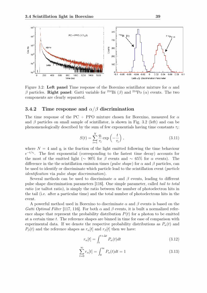
3.4 Scintillation light in Borexino 39
Figure 3.2: Left panel Time response of the Borexino scintillator mixture for α andβ particles. Right panel: Gatti variable for 214Bi (β) and 214Po (α) events. The twocomponents are clearly separated.
3.4.2 Time response and α/β discrimination
The time response of the PC + PPO mixture chosen for Borexino, measured for αand β particles on small sample of scintillator, is shown in Fig. 3.2 (left) and can bephenomenologically described by the sum of few exponentials having time constants τi:
S(t) =N∑i=1
qiτi
exp(− t
τi
), (3.11)
where N = 4 and qi is the fraction of the light emitted following the time behavioure−t/τi . The first exponential (corresponding to the fastest time decay) accounts forthe most of the emitted light (∼ 90% for β events and ∼ 65% for α events). Thedifference in the the scintillation emission times (pulse shape) for α and β particles, canbe used to identify or discriminate which particle lead to the scintillation event (particleidentification via pulse shape discrimination).
Several methods can be used to discriminate α and β events, leading to differentpulse shape discrimination parameters [116]. One simple parameter, called tail to totalratio (or tailtot ratio), is simply the ratio between the number of photoelectron hits inthe tail (i.e. after a particular time) and the total number of photoelectrons hits in theevent.
A powerful method used in Borexino to discriminate α and β events is based on theGatti Optimal Filter [117, 116]. For both α and β events, it is built a normalized refer-ence shape that represent the probability distribution P (t) for a photon to be emittedat a certain time t. The reference shapes are binned in time for ease of comparison withexperimental data. If we denote the respective probability distributions as Pα(t) andPβ(t) and the reference shapes as rα[t] and rβ[t] then we have:
rα[t] =∫ t+∆t
tPα(t)dt (3.12)
∞∑t=0
rα[t] =∫ ∞
0Pα(t)dt = 1 (3.13)

40 The Borexino experiment
where ∆t is the bin width. The same relations hold for rβ[t] and Pβ(t).The Gatti parameter for an event with a (binned and normalized) time profile e[t] is
then defined as:
ge ≡∞∑t=0
e[t] · w[t] (3.14)
wherew[t] ≡ rα[t]− rβ[t]
rα[t] + rβ[t]. (3.15)
For time bins where both reference shapes are zero, the weight w[t] is set to zero.Fig. 3.2 (right) shows the Gatti variable for the α and β samples obtained from the214Bi – 214Po fast coincidence decay. If an event with N photoelectrons is drawn fromthe α (β) probability distribution, then the corresponding Gatti parameter is also aprobability distribution Gα (Gβ). It can be shown that the mean and the variance ofthis distribution are
Gα =∞∑t=0
rα[t] · w[t] , (3.16)
var(Gα) =1
N
∞∑t=0
rα[t] · w2[t]− (Gα)2 , (3.17)
and the same equations hold for events drawn from the β probability time distribu-tion [117]. The absolute value for the means of the Gα and Gβ distributions are thesame (the differ in sign) and are independent of the number of photoelectrons N (i.e.on the energy of the event). These conditions are exactly true only if the event pulseshape is sampled for an infinite amount of time. For real data, sampled in a finite timewindow, the mean of the two distributions can be no longer equal in absolute value, andelectronic dead times and dark noise may lead to an energy dependence. The variance ofthe distributions are different and get large for low N , resulting in a worse α/β discrim-ination power at lower energy. More details and informations on the Gatti parameterand its implementation and usage in Borexino can be found in the PhD thesis [118] and[119].
3.4.3 Positron interactions and discrimination
The time profile of the scintillation and the quenching for a positron event is differentwith respect an electron event of the same energy. After the positron deposits its kineticenergy in the scintillator, the positron will annihilate with an electron, emitting twoback-to-back γ-rays. A slight difference in the time distribution of the scintillation signalarises from the time lag of few ns in the physical process of electron-positron annihilationas well as from the presence of annihilation γ-rays, which present a distributed, multi-siteevent topology and a larger average ionization density than electron interactions [120].
Prior to annihilation, the positron emitted in the 11C decay may form a bound statewith an electron in the scintillator, the positronium. The ground state of positroniumhas two possible configurations depending on the relative orientations of the spins ofthe electron and the positron: the spin singlet state (S = 0, MS = 0), called para-positronium (p-Ps), with a mean life of 125 ps in vacuum, and the spin triplet state

3.5 The Borexino energy spectrum 41
Photoelectrons [pe]100 200 300 400 500 600 700 800 900 1000
Counts / (5 pe x day x 100 tons)
-310
-210
-110
1
10
210
310
410
510All data after cuts (i) - (iii)
After cut (iv)
'sαAfter statistical subtraction of
Energy [keV]200 400 600 800 1000 1200 1400 1600
day
)]×
ton
×E
vent
Rat
e [e
vt /
(100
0 ke
V
-210
-110
1
10
210/NDF = 141/1382χFit:
1.5±Be: 45.5 .7
1.7±Kr: 34.8 .85
1.5±Bi: 41.5 .210
0.2±C: 28.9 .11
9.8±Po: 656.0 .210
0.7±External: 4.5 pp, pep, CNO (Fixed)
Figure 3.3: Left: The raw photoelectron charge spectrum after the basic cuts i-iii(black), after the fiducial volume cut i-iv (blue), and after the statistical subtractionof the α-emitting contaminants (red) (see Sec. 5.5.4). The description of the cuts isthe following: (i) muons and all events within a time window of 300 ms after a muonare rejected, (ii) events with multiple time clusters within the same hardware dataacquisition gate and events within 2 ms and 1.5 m of another event are rejected, (iii)noise and strange events are rejected, (iv) the reconstructed vertex is required to bewithin a 3.021 m fiducial radius and the vertex vertical distance from the detectorcentre is < 1.67 m. Right: A Monte Carlo based fit over the energy region 270-1600keV; the event energies are estimated using the number of photons detected by the PMTarray. Rate values in the legend are integrated over all energies and are quoted in unitsof counts/(day·100ton).
(S = 1, MS = -1, 0, 1), called ortho-positronium (o-Ps), with a mean lifetime invacuum equal to 140 ns. In liquid scintillator, however, the lifetime of o-Ps is reducedbecause of interactions with the surrounding medium: processes like spin-flip, or pick-off annihilation on collision with an anti-parallel spin electron, lead to the two bodydecay with lifetimes of a few nanoseconds. Laboratory measurements of o-Ps propertiescommon organic liquid scintillators leads to ∼ 3 ns mean life and ∼ 50% formationprobability [121]. The delay introduced by the o-Ps lifetime is comparable to to thefaster scintillation time constant (∼ 3 ns), and therefore is expected to introduce adistortion in the time distribution of hit PMTs with respect to a pure β− event ofthe same reconstructed energy. Additional distortions are expected from the diffusegeometry of events resulting from the positronium decay, due to the non-null free meanpath of the ensuing γ-rays.
More details on the β+/β− pulse shape discrimination performed in Borexino for themeasurement of the pep neutrino interaction rate can be found in Sec. 5.7.
3.5 The Borexino energy spectrum
An offline reconstruction code is employed in Borexino to reconstruct the time, theenergy, and the position of each recorded event. As a first step, the code identifyin the recorded gate the clusters, groups of time-correlated PMT hits that belong to
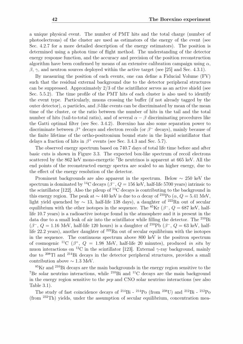
42 The Borexino experiment
a unique physical event. The number of PMT hits and the total charge (number ofphotoelectrons) of the cluster are used as estimators of the energy of the event (seeSec. 4.2.7 for a more detailed description of the energy estimators). The position isdetermined using a photon time of flight method. The understanding of the detectorenergy response function, and the accuracy and precision of the position reconstructionalgorithm have been confirmed by means of an extensive calibration campaign using α,β, γ, and neutron sources deployed within the active target (see [25] and Sec. 4.3.1).
By measuring the position of each events, one can define a Fiducial Volume (FV)such that the residual external background due to the detector peripheral structurescan be suppressed. Approximately 2/3 of the scintillator serves as an active shield (seeSec. 5.5.2). The time profile of the PMT hits of each cluster is also used to identifythe event type. Particularly, muons crossing the buffer (if not already tagged by theouter detector), α particles, and β-like events can be discriminated by mean of the meantime of the cluster, or the ratio between the number of hits in the tail and the totalnumber of hits (tail-to-total ratio), and of several α− β discriminating procedures likethe Gatti optimal filter (see Sec. 3.4.2). Borexino has also some separation power todiscriminate between β+ decays and electron recoils (or β− decays), mainly because ofthe finite lifetime of the ortho-positronium bound state in the liquid scintillator thatdelays a fraction of hits in β+ events (see Sec. 3.4.3 and Sec. 5.7).
The observed energy spectrum based on 740.7 days of total life time before and afterbasic cuts is shown in Figure 3.3. The expected box-like spectrum of recoil electronsscattered by the 862 keV mono-energetic 7Be neutrinos is apparent at 665 keV. All theend points of the reconstructed energy spectra are scaled to an higher energy, due tothe effect of the energy resolution of the detector.
Prominent backgrounds are also apparent in the spectrum. Below ∼ 250 keV thespectrum is dominated by 14C decays (β−, Q = 156 keV, half-life 5700 years) intrinsic tothe scintillator [122]. Also the pileup of 14C decays is contributing to the background inthis energy region. The peak at ∼ 440 keV is due to α decay of 210Po (α, Q = 5.41 MeV,light yield quenched by ∼ 13, half-life 138 days), a daughter of 222Rn out of secularequilibrium with the other isotopes in the sequence. The 85Kr (β−, Q = 687 keV, half-life 10.7 years) is a radioactive isotope found in the atmosphere and it is present in thedata due to a small leak of air into the scintillator while filling the detector. The 210Bi(β−, Q = 1.16 MeV, half-life 120 hours) is a daughter of 210Pb (β−, Q = 63 keV, half-life 22.2 years), another daughter of 222Rn out of secular equilibrium with the isotopesin the sequence. The continuous spectrum above 800 keV is the positron spectrumof cosmogenic 11C (β+, Q = 1.98 MeV, half-life 20 minutes), produced in situ bymuon interactions on 12C in the scintillator [123]. External γ-ray background, mainlydue to 208Tl and 214Bi decays in the detector peripheral structures, provides a smallcontribution above ∼ 1.3 MeV.
85Kr and 210Bi decays are the main backgrounds in the energy region sensitive to the7Be solar neutrino interactions, while 210Bi and 11C decays are the main backgroundin the energy region sensitive to the pep and CNO solar neutrino interactions (see alsoTable 3.1).
The study of fast coincidence decays of 214Bi - 214Po (from 238U) and 212Bi - 212Po(from 232Th) yields, under the assumption of secular equilibrium, concentration mea-

3.5 The Borexino energy spectrum 43
surements of (1.67± 0.06)× 10−17 g(238U)/g and (4.6± 0.8)× 10−17 g(232Th)/g in thescintillator. The 85Kr content in the scintillator is also probed through the rare decaysequence 85Kr → 85mRb + e− + νe, 85mRb → 85Rb + γ (τ = 1.5µs, BR 0.43%) thatoffers a delayed coincidence tag, and the resulting measurement for the activity of 85Kris (30.4± 5.3± 1.3) counts/(day·100ton) [25, 77].
The basic analysis method used in Borexino to evaluate the solar neutrino signal rateis a fit to the energy spectrum. In such fits, the weight for the solar neutrino signaland the main radioactive background components are left as free parameter. This isusually done for energy spectra constructed from both the number of PMTs hit and thetotal collected charge in the event [25]. The probability density functions (pdfs), thatare the energy reference spectra for the neutrino and radioactive background signalsused in the fit, are generated with two independent methods, one which is Monte Carlobased and one which uses an analytic modelling of the detector response. Usually, thefit to the energy spectrum constructed from the number of PMTs hit is performed withthe Monte Carlo based pdfs, while the fit to the energy spectrum constructed from thetotal charge is performed with the analytic based pdfs. Both methods benefit from anextensive campaign of detector calibrations. In order to perform precision measurementof the solar neutrino interaction rates, the modelling of the energy response functionmust be tuned with very high accuracy. The tuning of the Monte Carlo of the Borexinodetector, using the detector calibration data, has been one of my commitments withinthe Borexino collaboration. A description of the Borexino Monte Carlo, highlighted onthe tuning procedure and the accuracy obtained, is outlined in Chapter 4.
Although the simple fit to the energy spectrum has lead to the 5% precison mea-surement of the 7Be solar neutrino interaction rate [25], this analysis technique aloneis not sufficient to evidence the pep and CNO solar neutrino signals and measure theirinteraction rate, because of the high background rate due to the cosmogenic β+ emitter11C. Novel analysis procedures to suppress the 11C background have been developedand adopted for the pep and CNO solar neutrino analysis. Such techniques, whosedevelopment, application, and tuning have been part of my commitments within theBorexino collaboration, are described in Chapter 5.

Chapter 4
The Borexino detector response andsimulation
4.1 Introduction
The physics program of the Borexino experiment, in particular the solar neutrino de-tection, calls for an accurate and complete understanding of the detector response. Anhigh precision measurement of the 7Be solar neutrino flux, a measurement of 8B solarneutrinos with low energy threshold, a direct measurement of the rare signal from pepsolar neutrinos, and strong limits of the CNO solar neutrino flux all require a strict con-trol of detector stability, energy calibration, spatial reconstruction of the events, andpulse shape analysis.
This understanding was indeed achieved and implemented in a detailed full MonteCarlo simulation of the Borexino detector which now reproduces the data with accu-racy of 1% or better for all quantities relevant for data analysis. In order to reach theunderstanding and modelling of the Borexino detector response with high accuracy, anextensive calibration of the detector with α, β, γ, and neutron sources deployed in theactive target has been performed. Besides, a high activity 228Th source was deployedin the outermost buffer region, outside the active volume [124, 125]. These calibrationcampaigns have been crucial to develop, debug, upgrade, and fine-tune the full MonteCarlo simulation chain of Borexino. In particular, the calibration data has been instru-mental to validate the physics model used to describe the scintillation behaviour, thelight propagation, and the detector response to the light signal.
The upgrading, debugging, and tuning of the Monte Carlo simulation code has beenone of my commitments within the Borexino collaboration.
The full Monte Carlo simulation is extensively used in all the measurements in Borex-ino. For what concerns the pep and CNO solar neutrino measurement (see Chapter 5),the full Monte Carlo simulations have been used in particular for:
• generate the reference energy spectra for the neutrino signal and radioactive back-grounds used in the fits of the energy spectrum constructed from the numbers ofPMTs hit (see Sec. 3.5 and Sec. 5.9.2.2);
• generate the reference energy spectra and the spatial distribution profile of the
46 The Borexino detector response and simulation
external γ-ray background components (see Sec. 5.8);
• generate time profiles of the PMTs hit for electron and positron events to investi-gate the ortho-positronium formation in PC and study the feasibility of a β+-β−pulse shape discrimination in Borexino (see Sec. 5.7);
• generate the reference profile for many of the pulse shape discrimination variablesbased on the Gatti method (see Sec. 3.4.2 and Sec. 5.7.3).
Other use of the Monte Carlo simulations include the search for the best compromisebetween 11C rejection and fiducial exposure preservation in the TFC veto (see Sec. 5.5.3),the evaluation of the systematic uncertainties involved with the uncertainty in the energyresponse and in the position reconstruction (see Sec. 5.10.3), and the check of thereliability of the fit results and uncertainties with simulated event distributions (seeSec. 5.10.2).
The chapter is organised as follows. A description of the Borexino Monte Carlo chainand the physical models implemented therein are outlined in Sec. 4.2 of this chapter.In Sec. 4.3 I describe the tuning procedure used to tune the parameters of the energyand time response of the detector. The accuracy of the simulation is shown comparingreal and simulated calibration data.
4.2 The Monte Carlo simulation and the physics mod-elling of Borexino detector
Particles depositing energy in the Borexino Inner Vessel or in the buffer regions producescintillation and Cherenkov light which propagate inside the detector and eventuallyreach the PMTs, yielding a detectable signal.
For each event, the Borexino detector is measuring the number of photons detectedby each PMT, the charge of each photon hit and the relative time among hits of differentPMTs. The physical informations that can be extracted from the data are the amountof energy deposited in the scintillator (roughly proportional to the total number ofcollected hits or to the total integrated charge), the event position (making a time-of-flight fit to the time distribution of the hits), and, in some cases, the particle type, froma pulse shape analysis of the time scintillation signal pattern.
The accuracy in the modelling of the relation between the measured observables andthe physical quantities relies on the understanding of all the physical processes govern-ing the particle energy loss in the various materials, the scintillator light production,propagation and detection. Besides, it depends on the characteristics of the detectorelectronics and of the triggering system.
The Borexino full Monte Carlo simulation has been designed and optimised to fullymodel and reproduce all these processes up to the signal detection, providing simulatedevents in the very same format produced by real data acquisition. In this way, theevent reconstruction and analysis can be used on both real and simulated data, andblind analysis is in principle possible.
The full Monte Carlo simulation chain consists of a set of numerical codes that
4.2 The Monte Carlo simulation and the physics modelling ofBorexino detector 47
• generates the event (in particular, elastic scattering interactions based on thesolar neutrino spectrum, radioactive decays, calibration source events, muons andcosmogenic production, antineutrino interactions);
• simulates the energy loss of each specific particle in every material present in thedetector;
• generates the scintillation or Cherenkov photons from the particle energy loss inthe media and the property of the scintillator and the buffer;
• tracks each single scintillation photon including its interaction with the scintillatorand with the materials until a photomultiplier is reached or the photon is lost;
• generates the PMT pulse signal and the measured signals taking into account thespecific design of the front end and digital electronics chains of Borexino;
• simulates the trigger response and produce the final output for triggering events;
• produces a set of data formally identical to the real raw data.
These simulated data are then decoded and reconstructed with the same offline codeused for the real data.
The Borexino simulation chain is structured in three (or four) independent programs:
• GeNeb, an optional Fortran code for event generation and energy deposit.
• g4bx, a Geant41 based code for the event generation, energy loss, light generationand tracking.
• bx_elec, the electronics simulation code that simulates the trigger, the responseof the electronics and produces an output in the same format of the raw data.
• Echidna, the offline reconstruction code, which can be used to reconstruct simu-lated data in the same way of real data.
4.2.1 The event generation
Several event generators have been built within the Borexino Monte Carlo simulationcode, including generators for elastic scattering events of each solar neutrino compo-nent, radioactive decays (within the RDM module), calibrations sources, muons andcosmogenic production, neutrons, and antineutrino interactions.
1Geant4 is a object oriented C++ toolkit for the simulation of the passage of particles throughmatter. The tools of the package permits to build an accurate modelling of the detector geometry andmaterials [126].

48 The Borexino detector response and simulation
4.2.1.1 The solar neutrino generator
A special event generator that simulates elastic scattering interactions for each specieof solar neutrino has been developed in g4bx. The solar neutrino energy spectra aretaken from the computation of John Bahcall and his collaborators [127]. The oscillationeffects, which turns some νe into νµ or ντ are included. The electron neutrino survivalprobability (Pee) is calculated in the framework of the LMA-MSW oscillations (seeSec. 2.7). The solar neutrino generator simulates the flavour conversion according tothe energy of the neutrino and the oscillation parameters ∆m2
sun and θsun given asinput. The Sun matter effects are computed according to [128]. The kinetic energy ofthe electron recoils are randomly extracted according to Eq. 3.5.
4.2.1.2 The radioactive decay generators
Several radioactive decay generators are available in the Borexino Monte Carlo frame-work. One generator is implemented within the Fortran code GeNeb, originally devel-oped at the beginning of the project and extensively used during the CTF runs in the’90s to prove the feasibility of the experiment. GeNeb can generate each radioactivechain and computes the energy deposit for α, β and γ particles in the scintillator usingthe EGS4 library.
In g4bx, the main radioactive decay generator is Radioactive Decay Module (RDM)implemented within Geant4. RDM and the associated classes are used to simulate thedecay of radioactive nuclei by α, β± and γ emission and by electron capture (EC).The simulation model is empirical and data-driven, and uses the Evaluated NuclearStructure Data File (ENSDF, [129]). If the daughter of a nuclear decay is an excitedisomer, its prompt de-excitation is treated.
Another radioactive decay generator in g4bx is the custom SCS generator, which isused to generate “by hand" the energy spectra of some nuclear decays. The SCS modelis used do generate the spectral shapes which are wrongly implemented on RDM, orwhich have different references in literature, like 14C or 210Bi. More details on theGeNeb, RDM and SCS generators, as well as figures with energy spectra can be foundin the Borexino internal note [130].
4.2.1.3 The positron generator
Special care was devoted to generate positrons interactions. As described in Sec-tion 3.4.3, in a fraction of the cases, positrons are captured by electrons before an-nihilation and form positronium [120]. The positronium may be created in the ortho-positronium (o-Ps) state, which has a mean life in the scintillator of ∼ 3 ns [121],comparable to the faster scintillation constant. This effect delays the annihilation, thefurther energy deposit of the annihilation γ-rays, and the corresponding scintillationemission. o-Ps decays in 2 γ-rays because of the peak off effect.
The life time of ortho-positronium in PC+PPO mixture was measured in [121] andis ∼3 ns while the ortho-positronium formation probability was found to be ∼50%.The o-Ps generation and the related delay in the annihilation γ-rays interactions havesignificant impact on the emission time of the detected scintillation light (pulse shape).
4.2 The Monte Carlo simulation and the physics modelling ofBorexino detector 49
The difference in the pulse shape of an electron event with respect to a positron eventhas been be used to discriminate β− decay (or e− recoils) from the 11C β+ decay (seeSec. 5.7).
A special event generator that simulates this effect has been developed. Accordingto the input o-Ps formation probability, the code generates positron annihilations andpositronium decays. The latter process is simulated as a three-body vertex, composedby an electron, and two delayed annihilation gammas. The use of electrons instead ofpositrons is an approximation aimed to simplify the simulation, and motivated by thealmost identical energy losses, with the exception of the annihilation process. The delayof the gamma generation is ruled by an exponential law depending on the o-Ps meanlife, given as input.
4.2.1.4 The calibration source generator
Great care was devoted to the simulation of the γ and neutron calibration source runs(see Sec. 4.3.1). The construction of the quartz vial and the water solution containingthe radioactive source is included in the detector geometry and material construction.The calibration source is simulated in its real position, given as input. The decay of theradioactive source is simulated taking into account the correct branches of the decay.
4.2.2 The energy loss
The tools of the Geant4 package implemented within the Borexino Montecarlo Codeallow to build an accurate modelling of the detector geometry and materials: the outertank, Stainless Steel sphere, nylon vessels, photomultipliers and light cones, are con-structed with real sizes and material compositions. Special tools have been added totake into account the real shape of the Inner Vessel and its time dependent deviationsfrom a spherical shape.
The Geant4 libraries simulate the energy loss of each type of particle in every materialof the detector (scintillator, quencher, water, nylon, aluminium, steel). The relativelow energy of the typical events in Borexino make the tracking of each daughter (i.e.Compton electrons or e+e− pairs in γ-rays interactions) possible and preferable, allowingin principle high accuracy in the predictions. The standard Geant4 libraries are usedfor these processes. The stopping range of α particles is very short and can be neglectedin the simulation, so the energy loss is effectively point-like.
4.2.3 The light generation
Two distinct physical processes generate light in the Borexino detector: the scintillationprocess and the Cherenkov process. The former is the dominating process, being theCherenkov contribution at the level of ∼ 10% for an electron of ∼ 1 MeV. Within g4bx,special modules generate scintillation and Cherenkov optical photons according to theparticle type and the deposited energy. A large part of the Monte Carlo tuning thatwe have performed is involving the scintillation photon yield, the quenching effect, andthe time distribution of the emitted scintillation light.
50 The Borexino detector response and simulation
4.2.3.1 Scintillation light
The amount and time distribution of the emitted scintillation photons depend on variousmolecular processes taking place as a consequence of the particle energy loss. Thephysics mechanisms involved in the scintillation process are outlined in Section 3.4, andmore details can be found in the textbook [115].
The emission of light can not be simulated ab initio (i.e. at molecular level), becausetoo many molecules and processes should be taken into account, resulting in an imprac-tical simulation time. In the Borexino Monte Carlo, the emission of scintillation lightis modelled in a semi-empirical way.
The mean number optical photons emitted in the scintillation process is first com-puted from the primary particle (e− or α) energy loss, including the quenching effect.The scintillation model used in the Borexino Monte Carlo is the semi-empirical Birksmodel [115]. The Birks model relates the scintillation emission to the average ioniza-tion particle energy loss, dE/dx, and on the phenomenological Birks parameter kB.The Birks parameter depends on the scintillator composition and properties, and onthe length of the acquisition time. For most of the organic scintillators and setups, kBis of the order of 10−2 cm/MeV, but its precise value cannot be predicted, and has tobe determined experimentally. It is not still clear whether the Birks parameter have tobe the same for different type of particles. In Borexino, we define a Birks parameterfor each particle type, and we tuned it independently on the others. It turned out thatBirks parameters for different particle type have very similar values. The Birks semi-empirical formula yields the scintillation light yield dL produced when a particle loosesenergy in a distance dx with the stopping power dE/dx:
dL
dx=
L0dE/dx
1 + kB · dE/dx(4.1)
The Birks parametrisation is a macroscopic description of quenching, and can not beused directly in a stochastic approach as in Monte Carlo simulations. In the Birks model,in fact, the quenching effect is obtained by comparing the initial energy of the primaryparticle with the energy deposited in the detector. In particular, all energy deposits dueto secondaries produced by the primary particle (like δ-rays or X-rays) are assumed tobelong to the primary. On the other side, in the Monte Carlo approach, each particleis treated independently. A correct parametrisation of the Birks formalism requirestherefore to make the model compatible in a Geant4 framework, by evaluating thequenching factor for the primary ionizing particle, and inheriting the same factor to eachdaughter. The ingredients for this simulation approach are: an a priori parametrisationof the energy loss, required by the Birks equation, and a table of quenching factors asfunction of the energy, built at the initialisation phase, to speed up the simulation.
The mean number of emitted scintillation photons is obtained integrating Eq. 4.1 onthe particle range:
L(E) = L0
∫ E
0
dE
1 + kB · dE/dx(4.2)
One of the limiting case of Eq. 4.1 is kB · dE/dx � 1: in such cases, the light yield

4.2 The Monte Carlo simulation and the physics modelling ofBorexino detector 51
L(E) is approximately proportional to the particle energy loss ∆E:
L(E) ' L0∆E . (4.3)
This is a relatively good approximation for electrons of few MeV.When the denominator in Eq. 4.2 differ significantly from 1, the light yield is lower
than in Eq. 4.3, yielding an intrinsic non linearity between the energy loss ∆E andthe emitted scintillation L(E). This non linearity has to be properly modelled andaccounted in the data analysis. In the Birks model, the quenching factor Q(E), that isthe ratio between the true light yield and the one expected from the simple linear law4.3, assume the form (see Eq. 3.9)
Q(E) =1
E
∫ E
0
dE
1 + kBdE/dx(4.4)
and it is always lower than one. The deviation of the measured light yield from Eq. 4.3is increasingly important for protons, α particles, and nuclear fragments due to thehigh ionization per unit length. The quenching effect is also important for electronsand γ-rays with energy below few hundreds keV, as described in Sec. 3.4.1). The twoparameters used to model the scintillation and the quenching L0 and kB are not knowna priori, and are obtained by comparison between simulated data and the measured one(see Sec. 4.3.3)
For every electrons with energy E the mean number of scintillation photons to gen-erate is computed in g4bx through Eq. 3.9 with Q(E) given by Eq. 4.4 and obtainedusing the expression of dE/dx reported in [131] including the correction for positrons.The accuracy of dE/dx at very low energies (below and around 10 keV) is a subject ofscientific debate still in progress [132].
The number of scintillation photon to generate is then randomly fluctuated accordingto the Poisson statistics. The wavelength of the each scintillation photon is generatedaccording to the measured emission spectrum of the PC+PPO (1.5 g/l) scintillatormixture or PC+DMP buffer liquid [109]. The emission time of each scintillation pho-ton is randomly generated according to the semi-phenomenologically response of thescintillator, Eq. 3.11, with different parameters for α and β particles (see Sec. 3.4.2 andSec. 4.3.2).
4.2.3.2 Cherenkov light
Cherenkov photons are generated according to the Frank Tamm law in the wavelengthrange between 245 nm and 1800 nm. Ultraviolet Cherenkov photons that would not bedirectly detected by the photomultipliers are also generated and tracked: they can beabsorbed by the PC or PPO and reemitted at higher wave length and thus they canoriginate detectable signals.
4.2.4 The light tracking
Each optical photon is individually tracked applying of all relevant physics processes(emission, absorption and re-emission, scattering on molecules, reflection on surfaces,
52 The Borexino detector response and simulation
refraction between different media and absorption), allowing in principle high accuracyin the predictions.
Photon tracking takes into account the interactions of the emitted photons witheach single component of the scintillator and or the buffer. These processes includeelastic Rayleigh scattering of photons, absorption and re-emission of photons on PPOmolecules, absorption of photons by DMP molecules and also photon absorption in thinnylon vessels. The cross-sections (or equivalently the wavelength dependent attenuationlength Λ(λ)) for these interactions have been obtained from measurements of the ex-tinction coefficient as a function of the wavelength [111] while the scintillator refractionindex has been measured with a reflectometer.
In our model the light absorbed by PPO molecules is re-emitted with the probabilityQ=0.82 if the wavelength of the absorbed photon is lower than 375 nm and Q=0.15 forwavelength higher than 375 nm. We assume that the light is re-emitted in the IV withthe PPO emission spectrum. The re-emitted photons are modelled with an isotropicdistribution and emission mean time τ = 1.1 ns.
Interaction of light with PC for λ > 310 nm is simulated as Rayleigh scattering withan angular distribution P(θ) = 1 + cos2(θ), without time delay, and with no shift inthe wavelengths of emitted photons. At shorter wavelengths the interaction with PCis simulated as attraction by PC molecules with the following energy transfer to PPOand re-emission by PPO with probability Q=0.4 and emission time τ = 2.7 ns.
In buffer medium the light interacts with DMP molecules also as with the PC. Theinteraction with DMP leads to full photons absorption. Interaction with the PC isconsidered as Rayleigh scattering for λ > 310 nm. At shorter wavelengths the interac-tion with PC is simulated as attraction by PC molecules followed by re-emission withprobability Q=0.04 with buffer scintillation spectrum and emission time τ = 2.8 ns.
This light propagation model was already validated in CTF detector [111].The Geant4 code optical photon simulation takes into account the Borexino detector
optical surfaces and the processes of light reflection and refraction such as reflection oflight from the PMT photocathodes, PMT aluminium light guides, stainless steel vessel,refraction of light on the borders of scintillator, nylon vessels and pseudocumene buffer.Finally photons are detected by PMT with a probability following the wavelength de-pendence of photomultipliers quantum efficiency.
4.2.5 Photomultipliers and light guides
Amodel for photomultiplier tubes (PMTs) is implemented in g4bx code to fasten the cal-culations: the segment of sphere with photocathode surface and the aluminium cylinderto model the PMT backup. All PMTs installed in the detector are build in the simula-tion in their exact positions. The optical photons are detected taking into account themeasured wavelength dependences of PMT quantum efficiency and the relative PMTquantum efficiency of each PMT. The quantum efficiency of Borexino PMTs as a func-tion of wavelength was measured with laser techniques [113] before PMT installationinto Borexino and checked during detector operation period.
The polished aluminium lightgudes [133] and the reflection of photons from the lightguide surfaces also simulated.
4.2 The Monte Carlo simulation and the physics modelling ofBorexino detector 53
For each each photon detected (hit), the time of the hit and the PMT logical numberare written to the output of g4bx. The PMT logical number describes the real logicalelectronics channel and PMT position in the detector. The simulation of PMT responseto detected photons is done in bx_elec, the electronics part of the Borexino MonteCarlosimulation code.
4.2.6 The electronic simulation
The Geant4 code g4bx produces an output with the list of photons that gave a signalin a PMT, and the list of the hit times. Another C++ program, bx_elec, simulatesthe electronics chain and the triggering system, producing as an output a file formallyidentical to real data for all events that met the trigger conditions. The description ofbx_elec is outlined of this section.
The electronics simulation program first includes the effect of the PMT transit timespread (approximately a gaussian with σ ∼ 1 ns and a second peak at 60 ns) andincludes the after-pulse signal with a fixed probability of 2.5%. The after-pulse signalwas measured for all PMTs in a dark-room before installation in Borexino. Then, thehits due to PMT dark noise are using an average value equal to the measured one inthe real data run. The typical dark noise rate is below 1 kHz for most of the PMTs.In the real detector, all PMTs are carefully aligned in time by means of a laser pulsethat is synchronously delivered to each photocathode. This laser pulse is fired every0.5 ns in all runs, so that alignment can be continually monitored. The accuracy of thealignment is better than PMT time jitter, so no other effect must be included in thesimulation.
Then the code simulates the response of the electronics chain. Borexino electronicsis made by an analogue front end and a digital board which works both as a TDC andas an ADC [96].
The analogue board provides two signals: a linear amplification of the PMT signal,and a gate-less integrated signal. The first linear signal is discriminated by the digitalboard to measure the time of the pulse (with 0.5 ns resolution), while the integratedsignal is sampled by the ADC to measure the charge of each pulse. The integratorcircuit is such that the signal is almost constant for 80 ns after the pulse, and thendecays with a time constant of 500 ns because of the AC coupling between PMT andfront-end. In order to minimise the noise in the charge measurement, when the linearsignal goes above the discriminator threshold, the integrated signal is sampled twicewith an 8-bit ADC, once before the signal rise and a second time after 80 ns. The realcharge is proportional to the difference of these two ADC values. After each hit thedigital board is dead for approximately 140 ns. This means that when two hits closerthan 140 ns hit the same PMT, the second hit is lost for the time information. If thetime difference is less than 80 ns the charge measurement of the detected hit will bedoubled, while in the interval between 80 and 140 ns the second hit is completely lost.Although the frequency of multiple hits in the same PMT is rather small, especially atlow energy, this effect must be accurately simulated to reproduce the energy responseof the detector. The frequency of double hits depends on the event position (if thescintillation event is close to a group of PMTs, these see more light and the frequency
54 The Borexino detector response and simulation
is higher) and on the energy, introducing a small non linearity and non uniformity thatmust be included in the analysis.
The electronics simulation code generates the charge associated to the pulse using anexponential plus a gaussian distribution to reproduce the single photoelectron responseof the PMTs. The specific parameters for each PMT and the weight of the two con-tributions (different in the case of dark noise events and real scintillation events) havebeen obtained from the analysis of the real data. Then a PMT pulse with that charge isgenerated using a trapezoidal shape to approximate the rise and fall time of the signal,and the crossing of the discriminator threshold is simulated.
The program handles the front end behaviour properly summing the charge of thepulse produced on the same PMT within the 80 ns integration time; it takes also intoaccount "the pileup effect" of the integrator output, i.e. the fact that a pulse detected ona given channel produces a raise of the integrator baseline and a following exponentialdecay that influences the measurement of the charge of the following pulses. The 140 nsdead time is of course included in the simulation.
A physical trigger in Borexino and in the Monte Carlo happens when NThr hitsare detected within a time window ∆t. Typically NThr=25 and ∆t=100 ns. TheMonte Carlo reproduces also the time structure of the acquired data which is dueto details of the design of the digital board. In fact when the trigger is generatedall the hits happening in a time window (acquisition gate) having typically 16 µs ofduration are acquired. This is a time about 10 times longer than the maximum expectedduration of a single physical scintillation event. The acquisition gate contains the truescintillation event and several dark noise hits happening before and after the trigger.Multiple scintillation events due to fast radioactive decays may produce events with hitsin the same gate and this effect is properly simulated in the Monte Carlo. Additionalinformations present in the real data like the generation of the GPS time are alsoincluded in the code.
Finally, the code is also capable of including the effect of noisy and bad channels.During normal data taking, a dedicated program makes a complete check of the elec-tronics during the run, and store into a data base the list of dead or noisy channels. Theelectronics simulation program reads this data base and can therefore simulate a runin the same running condition. This is particularly important to correct for detectorinstabilities. All simulations used for physics analysis are therefore done simulating thereal Borexino detector, and not the ideal one.
4.2.7 The reconstruction program
The principal features of the Borexino reconstruction program (Echidna, and the addi-tional high level reconstruction step MOE) are outlined in Sec. 3.5.
Three basic energy estimators are available (both in the data and in the MonteCarlo):
• npmts: the number of PMTs having at least one hit.
• nhits: the number of hits detected by the electronics. Multiple hits on the samePMT are included if their time distance is higher than 140 ns.
4.3 The tuning of the Borexino Monte Carlo 55
• charge (npe): the sum of the charge of signal of every PMT as measured by thedigital boards (taking into account the 80 ns integration time and dead time)and normalized, for each PMT, to the peak position of each single photoelectronresponse.
These three basic energy estimator can then be implemented in several ways, depend-ing on the considered length of the cluster (either fixed or variable), the presence ofadditional dead time after the 140 ns to remove spurious hit due to re-triggering, andthe application of the subtraction of the expected dark noise hits.
The variables used in the pep ν and CNO νs analysis are described in Sec. 5.6.
4.3 The tuning of the Borexino Monte Carlo
The simulation of the scintillation and the optical process requires a large number ofparameters to be fixed and given as input to the Monte Carlo code. Such parametersdetermine the way physical and electronics processes take place in the simulation, andin the end, they are responsible of the output of the simulation, such as the timedistribution of hit PMTs and the total number of hit PMTs. The understanding of suchprocesses and the tuning of the corresponding models and parameters in the simulationleads to the understanding of the detector energy and time response, allowing highprecision measurements, like the 7Be solar neutrino flux [25], and measurements of raresignals, like the pep and CNO solar neutrino interactions (see chapter 5).
In order to reach the understanding and modelling of the Borexino detector responsewith high accuracy, an extensive calibration of the detector with α, β, γ, and neutronsources deployed in the scintillator active target has been performed after one year anda half of data taking (see Sec. 4.3.1 and the PhD thesis [134] for more details). Theset of calibration campaigns, which I participated, have been completed in November2008, January 2009, and June and July 2009. Besides, a high activity 228Th source wasdeployed in July 2010 in the outermost buffer region, outside the active volume [124,125].
The goal of the Borexino calibration campaigns was in particular to:
• Measure the accuracy of the event position reconstruction for events generatedin the whole vessel and in the energy range from about Emin ' 100 keV up toEmax ' 7 MeV.
• Measure the resolution of the event position reconstruction as a function of theevent position and energy.
• Calibrate the absolute energy scale from ∼ 100 keV to ∼ 7 MeV, with particularemphasis in the 7Be ν and pep ν energy region, i.e. ∼ 200 keV up to ∼ 2 MeV.
• Measure the energy resolution.
• Measure the non-uniformity of the energy response as a function of the eventposition and of the energy.
56 The Borexino detector response and simulation
• Check the effect of the external background.
The accuracy of the event position reconstruction is important for all solar neutrinomeasurements. The real neutrino target is a fiducial volume (FV) defined by softwarecuts on the reconstructed event position (see Sec. 5.5.2). A bias or a non uniform re-sponse in energy or position can bias the measured spectrum and lead to the systematicerrors.
Spectral distortions due to non-linearity or position dependence of the energy resolu-tion (see Sec. 5.5.2.2) are also crucial, and the absolute energy calibration is particularlyimportant to disentangle the 7Be ν signal from the 85Kr background and the pep ν signalfrom the 210Bi background.
Finally, the external background, is a non negligible contribution in the energy regionabove one MeV and is therefore important for the pep CNO and 8B neutrinos. A preciseknowledge and understanding of this background is mandatory in order to use a largerfiducial volume (see Sec. 5.5.2 and Sec. 5.8).
The calibration campaign of Borexino provided a clean sample of data that has beenused to check the accuracy of the results of Borexino Monte Carlo code and to preciselytune the values of the relevant parameter in the simulation of the physics and electronicsprocess. The parameters that have been optimised are:
• The absolute scintillator photon yield L0 (see Sec. 3.4). This is expected to bein the range ∼ 104 photons/MeV but its precise value has to be experimentallydetermined.
• The kB quenching factor for β, α and protons (see Sec. 3.4.1).
• The values of the scintillation parameters that describe its time response τi andqi (see Sec. 3.4.2 and Eq. 3.11).
• The reflection probability of the sphere and of the surface of the concentrators.
• The PPO re-emission probability.
• A scaling factor for the PPO and PC attenuation lengths.
• The after-pulse probability (see Sec. 4.2.6).
• A global scale factor in the PMT gain (see Sec. 4.2.6).
Optimising the simulation of the time response and light output means defining theset of values of the scintillation and optical parameter that gives the best accordancewith calibration source data. The time response and light output cannot be tuned inde-pendently because almost all of the listed parameters influence the energy estimators.We have used an iterative and recursive approach in which the agreement between thesimulated and measured time curves is searched with fixed light yield and kB and thenthese parameters are optimised again.

4.3 The tuning of the Borexino Monte Carlo 57
Isotope Type Energy (keV) activity (Bq)57Co γ 122 3.45 ± 0.07139Ce γ 165 3.12 ± 0.04203Hg γ 279 2.78 ± 0.0685Sr γ 514 -54Mn γ 834 -65Zn γ 1115 -60Co γ 1173 - 1332 -40K γ 1460 -222Rn α β 0-3200 -14C β 0-156 -241Am-9Be neutrons 2223 (H) - 4946 (12C) -
Table 4.1: Calibrations sources. In the 85Am–9Be source row, the quoted energy is theone of the capture γ-ray on the isotope in brackets.
4.3.1 The calibration data
Several radioactive sources have been deployed within the Inner Vessel (IV) by meansof a carefully designed insertion system [134]. The sources were selected in order tostudy the detector response in the energy region between 122 keV and 7 MeV with α,β, γ and neutrons. Table 4.1 shows the main parameters of the sources used. The char-acterisation of the detector cover both the energy range for solar neutrino spectroscopyand the whole fiducial volume.
Despite of the relatively large detector mass, the interaction rate for solar neutrinosin Borexino is of the order of a few tens of counts/(day·100ton) or even less thanone counts/(day·100ton), depending on the solar neutrino component (see Sec. 3.2 andTable 3.1). The low signal rate set very strong requirements on the background inducedthe radio-purity of all materials that have to be inserted in the detector itself. Particularcare has been therefore devoted to the preparation and handling of the calibrationsources and of the related insertion system as described in the PhD thesis [134] to ensurethat the radio-purity reached by Borexino [25, 77, 78] is not spoilt by the calibrationprocedure.
In order to calibrate the detector without introducing unwanted contaminations, thesource containers have been carefully designed. We have used a quartz sphere (one inchdiameter) either filled by 222Rn loaded scintillator identical to the Borexino or filled withγ emitters in aqueous solution. The quartz sphere were attached to a set of stainlesssteel bars that allowed to locate the source in almost any position within the IV (seethe PhD thesis [134]).
A special procedure was developed to minimise the quenching of the scintillationlight by oxygen. The comparison of the 210Po peak due to source events with the onedue to real 214BiPo coincidence in the detector shows that the result was quite goodand that the light quenching in the source was small.
The β and α events from the 222Rn source have been used to study the accuracy of

58 The Borexino detector response and simulation
the position reconstruction and the uniformity of the energy response as a function ofthe event position. The γ lines have provided the absolute energy scale along the wholeregion of interest.
In addition we have used a commercial 85Am–9Be neutron source. The α decay of241Am produces a 59.5 keV x-ray with a 36% branching ratio. Because of this x-rayactivity (about 180 kBq), too high for the data acquisition system, it was necessaryto shield the source. To avoid any contact between lead and the scintillator, a specialholder was fabricated: the body is white delrin, and the lead shielding is epoxied intothe interior faces of the holder; stainless steel hardware and a Viton o-ring seal theholder to avoid any contact between the scintillator and the source itself.
The sources have been deployed along the vertical z axis of the inner vessel andin several position off axis. An optical system made by a led mounted on the sourcesupport and a series of camera allows to know the position of the source in the innervessel with 2 cm accuracy. For more details about the sources, the deployment systemand the location of the sources with the cameras see the PhD thesis [134].
4.3.2 Tuning of the time response
The time distribution of hits is involved in the reconstruction of the main featuresof the event: the clustering and the total number of hits in the event, the positionreconstruction, the particle identification using pulse shape discrimination algorithms(see Sec. 3.4.2 and Sec. 3.5). In order to be able to simulated these high-level features,the time distribution of the hit PMTs (henceforth time distributions) must be simulatedwith at least 5% agreement with data, for each time bin and in the energy range usedin the analysis. In particular, the mean and the peak of the time distribution should bereproduced with 1 ns accuracy, and the other momenta of the distribution should notdisagree more then few nanosecond.
The parameters that influences the most the time distribution are: the scintillationparameters (τi, qi), the PPO re-emission probability, the scaling factors for the PPOand PC attenuation lengths, the reflection probability of the SSS, concentrators andPMT cathode. The Scintillation light parameters (τi, qi) are the one with the largestimpact on the shape of the time distribution: they affect the profile from the firstnanoseconds to tail of the distribution. PC and PPO scaling factors and attenuationlengths and PPO re-emission probability affects the rise of the time distribution and thewidth of its peak. They are also responsible for the uniformity of the energy responserespect to the position of the event. The reflection probability of the source of the SSS,of the PMT concentrators and of PMT cathode affects the time distribution with asecondary structure of hits at 50-70 ns. For what concerns the simulation of the PMTSand the electronics (see Sec. 4.2.6), the parameters that affects the time distributionare the PMT transition time spread and the PMT afterpulse probability and its timedistribution. Both of them have been measured and included in the simulation. Thetransition time spread affects the rise time of the distribution and the width of itspeak, and it is responsible of a secondary bump at ∼ 60 ns after the peak. The PMTafterpulse affects the time distribution with secondary hits from 140 ns to the end ofthe pulse.
4.3 The tuning of the Borexino Monte Carlo 59
Most of these parameters, with the exception of the τi and qi for α events, havebeen fine-tuned using the following γ-ray source runs as reference: 85Sr in 8 positions,54Mn, 65Zn and 40K at centre and at z = ±3m. The use of calibration data providesa set of advantages: calibration source runs ensure high statistics samples of pure andmonochromatic and point-like events, allowing to study the dependence of the accuracyof the simulation of the time distribution with respect to the energy and position ofthe event. The ensemble of this source scans the relevant energy and position rangefor 7Be ν analysis. The γ-ray sources have been employed to optimise the simulationof the time distribution of β events because the time distributions of β and γ eventsare very similar. In fact, γ-rays undergo Compton scattering on the electrons of thescintillator. Recoil electrons loose energy and produce scintillation light. Hence, theγ-ray is detected as superpositions of electron events of lower energy, close in space andtime. Once the whole set of parameters have been tuned for β events, the α decay timesand weights have been tuned using 214Po events in 222Rn sources.
The following iterative procedure has been followed. From a given calibration datarun, the time distribution is built. The events coming from the calibration sourceare selected cutting events reconstructed outside a sphere of 1 m from the nominalsource position. Only events with reconstructed energy around the nominal energy onthe source are considered. Muons events and muon daughters are rejected using theexternal muon veto and the standard analysis cuts (see [105] and Sec. 5.5.1).
The very same calibration run is then simulated (see Sec. 4.2.1.4) with a given set ofoptical parameters. Great care was devoted to simulate the electronics configuration inthe same configuration of the real run. In particular we have included the pattern thePMTs that were disabled during the run, the measured dark noise of the PMTs, basedto the rate of random triggers during that run, the gain of each PMT, taken from tothe electronics calibrations of the real run. The procedure of event selection describedin the previous paragraph is performed on the simulated events. The time distributionsof the selected simulated events are then compared to the corresponding distributionfor real data events. For sources located at z = ±3 m from the centre of the detector,the time distributions are also compared using only the time distribution of hits in asubset of PMTs near or far from the source.
The optical parameters that leads to the best accordance between simulated andreal time distributions are then selected. The comparison is done with the method ofthe least squares. Direct comparison using the eyes (that are the best tool of patternrecognition at present time) is also performed to select the final choice of configurationparameters.
A final overall check for β and α time distributions is done using the sample given bythe 214BiPo coincidences on normal runs (see Sec. 3.5). These events are distributed inthe whole volume of the Inner Vessel. This allow to check the goodness of the simulationon the overall fiducial volume, instead of a point-like source. The inhomogeneity of theposition of 214BiPo events along the vertical axis is taken in account with the methodof rejection.

60 The Borexino detector response and simulation
4.3.3 Tuning of the energy response
The physics goals of the Borexino experiment (see Chapter 3) require to simulate theenergy estimators with ∼ 1% accuracy in the energy range 100 keV – 2 MeV relevantfor the 7Be ν analysis [25] and with a similar accuracy in the energy range 200 keV –2.6 MeV used in the pep ν analysis (see Chapter 5).
The tuning of the energy response is performed defining the photon yield L0 andthe Birks quenching parameter kB in the simulation that gives the best accordancewith data. For a given energy estimator (see Sec. 4.2.7), the ratio between the positionof the energy spectrum peaks of events with different energy is mostly related to thequenching factor kB, while the absolute energy scale is determined by L0. Being noneof the energy estimators described in exactly linearly related to the energy and to L0,then no rescaling of the simulation results is applied: we aim to reproduce the absolutevalues of the energy estimators with given L0 and kB.
The reproduction of the energy estimator npmts is related to the accuracy of themodels of the energy loss, light generation and interaction in the media. The energy es-timator nhits depends also on the accuracy of the electronics simulation (see Sec. 4.2.6),mostly because of the electronics dead time and the afterpulse. The charge (npe) energyestimator is also related to the accuracy of the simulation of the shape of the photomul-tiplier pulses and of the single photoelectron charge spectrum of each photomultiplier.
The tuning of the simulation of energy response is performed as follows. As a firststep, we tune the photon yield L0 and the Birks parameter kB with calibration sourceslocated in the centre of the detector (see Sec. 4.3.3.1). The tuning of the photonyield and the Birks parameter is performed mainly using the npmts and nhits energyestimator. The adjustment of the nhits and charge simulation, if needed, is obtained bytuning the parameters of the electronics code bx_elec (see Sec. 4.3.3.2). A comparisonwith 11C spectrum (tagged with the TFC method, see Sec. 5.5.3) is performed in order tounderstand the agreement of the simulation the whole fiducial volume (FV). If needed,an effective L0 for the simulation of the events in the FV is defined.
4.3.3.1 Tuning of the quenching for e− and γ-rays
The calibration sources used for the tuning of the energy response in the centre of thedetector are the γ emitter isotopes: 57Co, 139Ce, 203Hg, 85Sr, 54Mn, 65Zn, 60Co and 40K.Such sources allow the tuning of the simulation of the energy response for e± and γevents in the energy range between ∼ 60 keV and ∼ 2.4 MeV. Because of the quenchingeffect (see Sec. 3.4.1), the amount of light induced by a γ-ray is lower than the lightemitted by an electron of the same energy.
The cuts to select the γ-rays emitted by the calibration source in the centre of thedetector are the same described in Sec. 4.3.2. However, the energy of 57Co, 139Ce, and203Hg γ-rays lies below the high-rate 14C decay end point, and the position cut is notsufficient to remove 14C events. In order to obtain a clean spectrum of γ-ray eventsfor these source runs, a subtraction of background events must be done. A bin per binsubtraction of the average energy spectrum of the two normal runs just before and afterthe calibration run is performed. This procedure allows to remove the 14C and 210Podecay contamination in the calibration source γ-ray event sample with high accuracy.

4.3 The tuning of the Borexino Monte Carlo 61
)-1 Photon Yield / (photons MeV16000 16200 16400 16600 16800 17000
)-1
cm MeV
-4
/ (10
B Birks Parameter k
9092949698
100102104106108110112114
1
10
Gamma Peaks: ((DATA-MC))^2/(1 + Err DATA^2 + Err MC^2) for normalized npmts
)-1 Photon Yield / (photons MeV16000 16200 16400 16600 16800 17000
)-1
cm MeV
-4
/ (10
B Birks Parameter k
9092949698
100102104106108110112114
1
10
Gamma Peaks: ((DATA-MC))^2/(1 + Err DATA^2 + Err MC^2) for normalized nhits
Figure 4.1: Distribution of the estimator of the goodness of the simulation of the energyresponse (Eq. 4.5) for γ-ray sources in the centre of the detector, as a function of thephoton yield L0 and Birks parameter kB. Left panel: For the npmts energy estimator.Right panel: For the nhits energy estimator.
The very same calibration runs are then simulated (see Sec. 4.2.1.4) with a given (L0,kB) pair. The agreement between data and simulation is defined by the comparison ofthe reconstructed energy peak of each γ source. We fit the γ-peaks either with aGaussian or a generalised gamma distribution [135] plus a 2nd-order polynomium (tomodel irreducible background) in order to find the mean value and the resolution of theenergy estimator at the energy of the given γ-ray. We have defined an estimator of thegoodness of the energy simulation as:
1
N
∑sources
(µdata − µMC)2
1 + e2µdata + e2
µMC
(4.5)
where µ is the mean value given by the fit (i.e. the peak position of the γ-peak in theenergy spectrum) and eµ is its error, and the sum is extended to the total number ofconsidered calibration sources (N). The (L0, kB) pairs that give the best accordanceare defined looking for the minimum value of 4.5 in the bidimensional parameter spaceof L0 and kB. The distribution of the estimator of the goodness of the simulation, forthe last version of the Borexino simulation code, is shown in Fig. 4.1. Once a smallsubsample of good L0 and kB pairs are found, we perform χ2 tests of the γ-ray energyspectra between data and simulation in order to define the (L0, kB) that gives the bestaccordance. The energy spectrum of the calibration γ-ray sources in the centre of thedetector, for real and simulated calibration data is shown in Fig. 4.2.
The Birks quenching parameter kB is then selected and fixed in the next step of theenergy tuning, while the photon yield L0 is allowed to be scaled by a small factor inorder to correct volume effects, if needed.
4.3.3.2 Tuning of the electronics simulation parameters
The procedure outlined in Sec. 4.3.3.1 is performed on each energy estimator (npmts,nhits and charge, see Sec. 4.2.7). We tune the electronics simulation code (see Sec. 4.2.6)
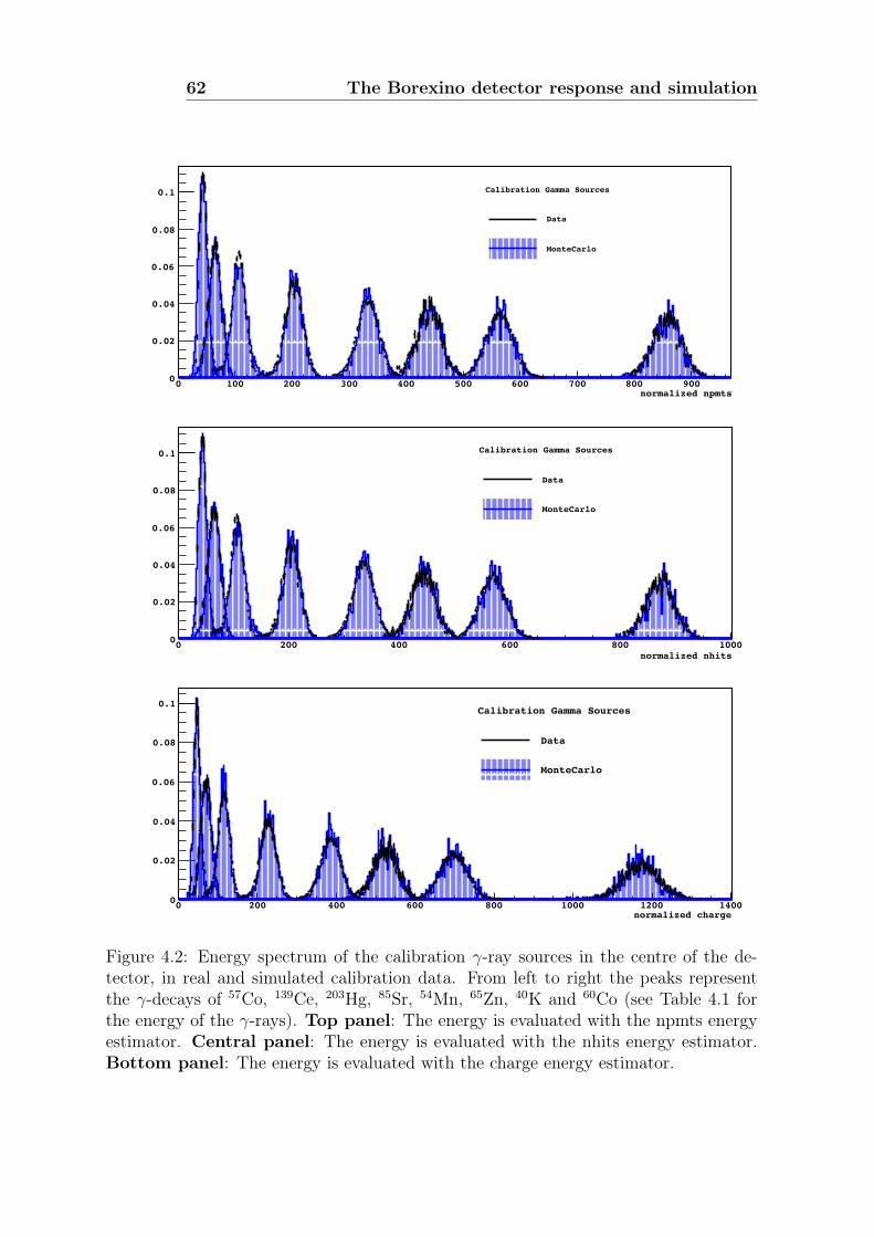
62 The Borexino detector response and simulation
normalized npmts0 100 200 300 400 500 600 700 800 9000
0.02
0.04
0.06
0.08
0.1 Calibration Gamma Sources
Data
MonteCarlo
normalized nhits0 200 400 600 800 10000
0.02
0.04
0.06
0.08
0.1 Calibration Gamma Sources
Data
MonteCarlo
normalized charge0 200 400 600 800 1000 1200 14000
0.02
0.04
0.06
0.08
0.1Calibration Gamma Sources
Data
MonteCarlo
Figure 4.2: Energy spectrum of the calibration γ-ray sources in the centre of the de-tector, in real and simulated calibration data. From left to right the peaks representthe γ-decays of 57Co, 139Ce, 203Hg, 85Sr, 54Mn, 65Zn, 40K and 60Co (see Table 4.1 forthe energy of the γ-rays). Top panel: The energy is evaluated with the npmts energyestimator. Central panel: The energy is evaluated with the nhits energy estimator.Bottom panel: The energy is evaluated with the charge energy estimator.
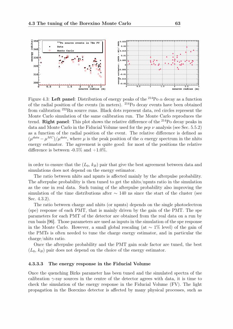
4.3 The tuning of the Borexino Monte Carlo 63
source radius (m)0 0.5 1 1.5 2 2.5 3
energy (nhits)
300
310
320
330
340
350
Po source events in 7Be FV214
Po source events in 7Be FV214
Data
Monte Carlo
source radius (m)0 0.5 1 1.5 2 2.5 3
energy estimator: (DATA - MC)/ DATA
-0.02
-0.015
-0.01
-0.005
0
0.005
0.01
0.015
0.02
0.025
(DATAmean_simple- MCmean_simple)/DATAmean_simple:(R) {(R<2.8) && (Z>-1.8) && (Z<2.2)}
Figure 4.3: Left panel: Distribution of energy peaks of the 214Po α decay as a functionof the radial position of the events (in meters). 214Po decay events have been obtainedfrom calibration 222Rn source runs. Black dots represent data, red circles represent theMonte Carlo simulation of the same calibration run. The Monte Carlo reproduces thetrend. Right panel: This plot shows the relative difference of the 214Po decay peaks indata and Monte Carlo in the Fiducial Volume used for the pep ν analysis (see Sec. 5.5.2)as a function of the radial position of the event. The relative difference is defined as(µdata−µMC)/µdata, where µ is the peak position of the α energy spectrum in the nhitsenergy estimator. The agreement is quite good: for most of the positions the relativedifference is between -0.5% and +1.0%.
in order to ensure that the (L0, kB) pair that give the best agreement between data andsimulations does not depend on the energy estimator.
The ratio between nhits and npmts is affected mainly by the afterpulse probability.The afterpulse probability is then tuned to get the nhits/npmts ratio in the simulationas the one in real data. Such tuning of the afterpulse probability also improving thesimulation of the time distributions after ∼ 140 ns since the start of the cluster (seeSec. 4.3.2).
The ratio between charge and nhits (or npmts) depends on the single photoelectron(spe) response of each PMT, that is mainly driven by the gain of the PMT. The speparameters for each PMT of the detector are obtained from the real data on a run byrun basis [96]. Those parameters are used as inputs in the simulation of the spe responsein the Monte Carlo. However, a small global rescaling (at ∼ 1% level) of the gain ofthe PMTs is often needed to tune the charge energy estimator, and in particular thecharge/nhits ratio.
Once the afterpulse probability and the PMT gain scale factor are tuned, the best(L0, kB) pair does not depend on the choice of the energy estimator.
4.3.3.3 The energy response in the Fiducial Volume
Once the quenching Birks parameter has been tuned and the simulated spectra of thecalibration γ-ray sources in the centre of the detector agrees with data, it is time tocheck the simulation of the energy response in the Fiducial Volume (FV). The lightpropagation in the Borexino detector is affected by many physical processes, such as
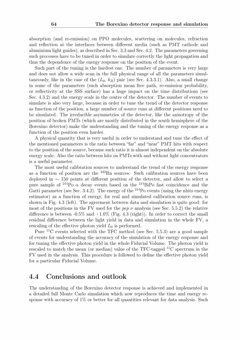
64 The Borexino detector response and simulation
absorption (and re-emission) on PPO molecules, scattering on molecules, refractionand reflection at the interfaces between different media (such as PMT cathode andaluminium light guides), as described in Sec. 3.3 and Sec. 4.2. The parameters governingsuch processes have to be tuned in order to simulate correctly the light propagation andthus the dependence of the energy response on the position of the event.
Such part of the tuning is the hardest one. The number of parameters is very largeand does not allow a wide scan in the full physical range of all the parameters simul-taneously, like in the case of the (L0, kB) pair (see Sec. 4.3.3.1). Also, a small changein some of the parameters (such absorption mean free path, re-emission probability,or reflectivity at the SSS surface) has a huge impact on the time distributions (seeSec. 4.3.2) and the energy scale in the centre of the detector. The number of events tosimulate is also very large, because in order to tune the trend of the detector responseas function of the position, a large number of source runs at different positions need tobe simulated. The irreducible asymmetries of the detector, like the anisotropy of theposition of broken PMTs (which are mostly distributed in the south hemisphere of theBorexino detector) make the understanding and the tuning of the energy response as afunction of the position even harder.
A physical quantity that is very useful in order to understand and tune the effect ofthe mentioned parameters is the ratio between “far” and “near” PMT hits with respectto the position of the source, because such ratio it is almost independent on the absoluteenergy scale. Also the ratio between hits on PMTs with and without light concentratorsis a useful parameter.
The most useful calibration sources to understand the trend of the energy responseas a function of position are the 222Rn sources. Such calibration sources have beendeployed in ∼ 150 points at different position of the detector, and allow to select apure sample of 214Po α decay events based on the 214BiPo fast coincidence and theGatti parameter (see Sec. 3.4.2). The energy of the 214Po events (using the nhits energyestimator) as a function of energy, for real and simulated calibration source runs, isshown in Fig. 4.3 (left). The agreement between data and simulation is quite good: formost of the positions in the FV used for the pep ν analysis (see Sec. 5.5.2) the relativedifference is between -0.5% and +1.0% (Fig. 4.3 (right)). In order to correct the smallresidual difference between the light yield in data and simulation in the whole FV, arescaling of the effective photon yield L0 is performed.
Pure 11C events selected with the TFC method (see Sec. 5.5.3) are a good sampleof events for understanding the accuracy of the simulation of the energy response andfor tuning the effective photon yield in the whole Fiducial Volume. The photon yield isrescaled to match the mean (or median) value of the TFC-tagged 11C spectrum in theFV used in the analysis. This procedure is followed to define the effective photon yieldfor a particular Fiducial Volume.
4.4 Conclusions and outlookThe understanding of the Borexino detector response is achieved and implemented ina detailed full Monte Carlo simulation which now reproduces the time and energy re-sponse with accuracy of 1% or better for all quantities relevant for data analysis. Such

4.4 Conclusions and outlook 65
understanding and accuracy is mandatory in order to pursue the physics goals of theBorexino experiment, like the direct measurement of the rare signal from pep solarneutrinos, and the limits of the CNO solar neutrino flux.


Chapter 5
Measurement of the pep and CNO solarneutrino interaction rates in Borexino
5.1 Introduction
I report on this chapter the first measurement of the pep solar neutrino interaction rateand the best limits on the CNO solar neutrino interaction rate in Borexino. The rate ofpep ν electron scattering interactions is determined to be 3.1 ± 0.6 (stat) ± 0.3 (syst)counts/(day·100ton). The upper limits on the CNO neutrino interaction rate at 68%(95%) C.L. are determined to be 4 (12) counts/(day·100ton). Assuming the pep neutrinoflux predicted by the Standard Solar Model, we obtained a constraint on the CNO solarneutrino interaction rate of <7.9 counts/(day·100ton) (95% C.L.). Assuming the MSW-LMA solution to solar neutrino oscillations, these values correspond to solar neutrinofluxes of (1.6±0.3)×108 cm−2s−1 and <7.7×108 cm−2s−1 (95% C.L.), respectively, inagreement with both the High and Low Metallicity Standard Solar Models. The absenceof the solar neutrino signal is disfavoured at 99.97% C.L., while the absence of the pepneutrino signal is disfavored at 98% C.L. These results represent the first direct evidenceof the pep neutrino signal and the strongest constraint of the CNO solar neutrino fluxto date.
The necessary sensitivity was achieved by adopting novel data analysis techniquesfor the rejection of cosmogenic 11C, the dominant background in the 1–2MeV region.As the signal to background ratio in the energy region of interest is orders of magnitudelower than for the 7Be ν analysis [25], new data selection, pulse shape and analysistechniques have been developed, and much smaller backgrounds have been considered.In this chapter I describe in detail the analysis performed.
The chapter is organised as follows. In Section 5.2 I review the pep ν and CNO νssignal in Borexino. In Section 5.3, all the relevant sources of physical backgrounds arediscussed and estimates for their rates presented. Section 5.4 and 5.5 report on the dataand event selection cuts implemented to obtain the final candidates for this analysis.Special care has been taken in the definition of the fiducial volume and in the descriptionof the three-fold coincidence (TFC) veto.
As in the 7Be ν analysis, the neutrino interaction rates are obtained from a fit tothe distributions of the final candidates. Thus, in Section 5.6 I define the variables to

68Measurement of the pep and CNO solar neutrino interaction rates
in Borexino
be used for the energy spectrum. In Section 5.7 I describe the procedure to obtain asingle pulse shape variable to effectively discriminate between β+ and β− events that isimplemented in the fit. In Section 5.8 I present the radial and energy distributions ofthe external γ-ray background, which are crucial components of the fit. The details ofthe fitting procedure are described in Section 5.9. The results of the analysis and thetests to validate the fitting strategy are presented in Section 5.10.
5.2 pep ν and CNO νs signalsThe energy spectra of solar neutrinos are shown in Fig. 2.1. The energy spectrum ofelectron recoils from ν−e elastic scattering interactions in Borexino is shown in Fig. 5.1(left). The kinetic energies of electron recoils from pep and CNO neutrino interactionsextend past the end-point of the 7Be ν electron recoil spectrum and are within therange of energies that can be measured by Borexino. The interaction rates from pepand CNO νs in Borexino are a few counts per day/100tons, ∼10 times lower thanthose from 7Be ν. The pep ν and CNO νs signal and energy spectrum are described inSec. 5.2.1 and Sec. 5.2.2 respectively.
5.2.1 pep ν signal
The pep ν is a mono-energetic solar neutrino with 1.44 MeV of energy. The pep reactionis part of the pp fusion chain, which is the main mechanism of energy production in theSun. The features of the pep reaction and the production of pep neutrinos are describedin Sec. 2.4.
The expected electron recoil energy spectrum from pep νs in Borexino is shown inFig. 5.1 (right). As with the mono-energetic 7Be ν the spectrum from pep ν interactionsis box-like, but with a higher end point and a considerably lower interaction rate (seeSec. 3.2, Table 3.1). The leading standard solar models (SSMs) predict an interactionrate of pep neutrinos in Borexino of 2.80± 0.04 (High Metallicity) and 2.86± 0.04 (LowMetallicity) cpd/100tons [60].
5.2.2 CNO νs signal
The CNO-cycle is an alternate mechanism of energy production in the Sun, where 12Cserve as catalysts in the fusion of four protons into a 4He nucleus. The features of theCNO reactions and the production of CNO neutrinos are discussed in Sec. 2.4.
The CNO cycle has two sub-cycles: the CN cycle and the sub-dominant NO cycle.In the CN cycle, 13N ν and 15O νs are produced, with continuous spectra with endpoint energies at 1.19 MeV and 1.73 MeV respectively. As every cycle produces exactlyone 13N ν and one 15O ν, their fluxes are very strongly correlated, with correlationcoefficients of 0.991(0.984) in the GS98(AGS05) standard solar model [58].
In a minor branch of this reaction, which occurs with a relative frequency of ∼2%,the final reaction does not end with the production of 12C + 4He, but instead continuesin the NO cycle. Here, an additional neutrino (17F ν) is produced with a Q-value thatis very close to that of the 15O ν. The spectra from 17F νs and 15O νs are very similar
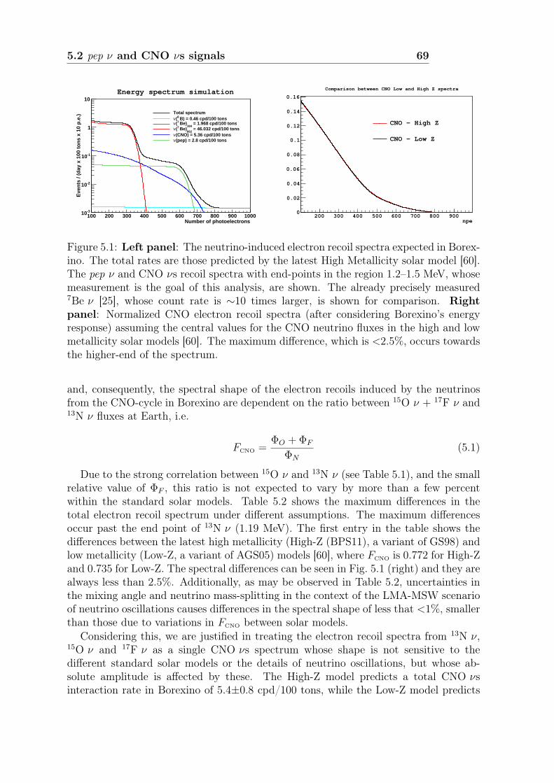
5.2 pep ν and CNO νs signals 69
Number of photoelectrons100 200 300 400 500 600 700 800 900 1000
Eve
nts
/ (d
ay x
100
to
ns
x 10
p.e
.)
-310
-210
-110
1
10
Total spectrumB) = 0.46 cpd/100 tons8 (ν
= 1.968 cpd/100 tons384
Be)7 (ν = 46.032 cpd/100 tons
862Be)7 (ν
(CNO) = 5.36 cpd/100 tonsν(pep) = 2.8 cpd/100 tonsν
Energy spectrum simulation
npe200 300 400 500 600 700 800 900
0
0.02
0.04
0.06
0.08
0.1
0.12
0.14
0.16
Comparison between CNO Low and High Z spectra
CNO - High Z
CNO - Low Z
Figure 5.1: Left panel: The neutrino-induced electron recoil spectra expected in Borex-ino. The total rates are those predicted by the latest High Metallicity solar model [60].The pep ν and CNO νs recoil spectra with end-points in the region 1.2–1.5 MeV, whosemeasurement is the goal of this analysis, are shown. The already precisely measured7Be ν [25], whose count rate is ∼10 times larger, is shown for comparison. Rightpanel: Normalized CNO electron recoil spectra (after considering Borexino’s energyresponse) assuming the central values for the CNO neutrino fluxes in the high and lowmetallicity solar models [60]. The maximum difference, which is <2.5%, occurs towardsthe higher-end of the spectrum.
and, consequently, the spectral shape of the electron recoils induced by the neutrinosfrom the CNO-cycle in Borexino are dependent on the ratio between 15O ν + 17F ν and13N ν fluxes at Earth, i.e.
FCNO =ΦO + ΦF
ΦN
(5.1)
Due to the strong correlation between 15O ν and 13N ν (see Table 5.1), and the smallrelative value of ΦF , this ratio is not expected to vary by more than a few percentwithin the standard solar models. Table 5.2 shows the maximum differences in thetotal electron recoil spectrum under different assumptions. The maximum differencesoccur past the end point of 13N ν (1.19 MeV). The first entry in the table shows thedifferences between the latest high metallicity (High-Z (BPS11), a variant of GS98) andlow metallicity (Low-Z, a variant of AGS05) models [60], where FCNO is 0.772 for High-Zand 0.735 for Low-Z. The spectral differences can be seen in Fig. 5.1 (right) and they arealways less than 2.5%. Additionally, as may be observed in Table 5.2, uncertainties inthe mixing angle and neutrino mass-splitting in the context of the LMA-MSW scenarioof neutrino oscillations causes differences in the spectral shape of less that <1%, smallerthan those due to variations in FCNO between solar models.
Considering this, we are justified in treating the electron recoil spectra from 13N ν,15O ν and 17F ν as a single CNO νs spectrum whose shape is not sensitive to thedifferent standard solar models or the details of neutrino oscillations, but whose ab-solute amplitude is affected by these. The High-Z model predicts a total CNO νsinteraction rate in Borexino of 5.4±0.8 cpd/100 tons, while the Low-Z model predicts

70Measurement of the pep and CNO solar neutrino interaction rates
in Borexino
Neutrino Flux at the Sun End point ρ(13N ν, j) ρ(15O ν, j) ρ(17F ν, j)/ 108 cm−2s−1 / MeV
13N ν 2.96 (2.17) 1.19 1 0.991 (0.984) 0.172 (0.299)15O ν 2.23 (1.56) 1.73 0.991 (0.984) 1 0.219 (0.338)17F ν 0.055 (0.034) 1.74 0.172 (0.299) 0.219 (0.338) 1
Table 5.1: The second column in this table shows the central values for the predictedfluxes of the neutrinos from the CNO cycle by the latest High-Z (Low-Z) solar models.The third column shows the maximum neutrino energy for the three types, while thefourth, fifth and sixth columns show the correlation coefficients, ρ(i, j), for the differentdecays, obtained from Tables 16 and 17 in [58]. Even though the total fluxes from neu-trinos from the CNO cycle is ∼30% smaller for the Low-Z model, the strong correlationbetween 13N ν and 15O ν, and the small relative flux from 17F ν, lead to relatively smallchanges in the electron recoil spectral shape (see Table 5.2).
Conditions Fractional diff. in normalizede− recoil npe spectrum from CNO νs
High-Z vs. Low-Z < 2.5%Central osc. pars. vs. +1σ in ∆m2 and θ [2] < 0.25%Central osc. pars. vs. −1σ in ∆m2 and θ [2] < 0.25%With vs. without Earth matter effects < 0.1%With vs. without radiative corrections < 1%
Table 5.2: This table shows the differences in the total electron recoil spectrum fromCNO neutrinos observed in Borexino under different model assumptions. The first entryshows the largest difference, which occurs between the high and low metallicity solarmodels [60] (see Fig. 5.1-right). The following three entries show that changes in theparameters of the LMA-MSW model of neutrino oscillations have a much smaller effectin the spectral shape relative to the differences between the solar models. Overall, thesmall spectral differences in the electron recoil spectrum from the model assumptionsintroduces a negligible systematic effect in the estimation of the total CNO neutrinointeraction rate in Borexino. For reference, the effect of radiative corrections in therecoil spectra is presented in the last entry.
5.3 Radioactive backgrounds 71
3.8+0.6−0.5 cpd/100 tons.
5.3 Radioactive backgrounds
As discussed in Sec. 5.2, the interaction rates for pep ν and CNO νs in Borexino are∼10 times lower than those from 7Be ν, whose measurement has been the main goal ofBorexino [25]. Because of this, special care needs to be taken to consider radioactivebackgrounds with rates that are one or two orders of magnitude lower than those ofrelevance for the 7Be ν analysis. Similarly to the 7Be ν analysis, the pep ν and CNO νsinteraction rates are obtained through a fit to the signal and background distributions indifferent parameter spaces (see Sec. 5.9) and, therefore it is of great importance to makeestimates of the possible radioactive contaminants in order to decide which should beconsidered for the fit. In Sec. 5.3.1, 5.3.2 and 5.3.3, the predicted rates for the differenttypes of backgrounds are evaluated in the fiducial volume (see Sec. 5.5.2) and energyrange of interest to decide which should be considered in this analysis.
5.3.1 Radiogenic internal backgrounds
The main radiogenic backgrounds for the 7Be ν analysis [25] are also the dominant back-grounds for this analysis. 85Kr, which has been measured from the delayed coincidenceanalysis to be 30.4 ± 5.3 ± 1.3 cpd/100tons [25] and 210Bi, whose value from the 7Beanalysis fit was 40.3 ± 1.5 ± 2.3 cpd/100tons, are the largest radioactive backgroundsto be included in the fit. 210Po, which has the highest rate of any of the internal con-taminants above the 14C end-point (∼2.1 cpd/ton [25]), is removed from the spectrumthrough the method of statistical subtraction, discussed in Sec. 5.5.4. The only remain-ing contribution from 210Po to the final spectrum is the γ-ray producing decay (0.8MeVγ + 4.5MeV α), which has a relative intensity of 0.00121%.
Similarly to the 7Be ν analysis, the 214Pb decay rate can be estimated from thenumber of detected fast 214BiPo coincidences in the analysis exposure [25, 96]. Forthe exposure considered in the 7Be ν analysis, the 214Pb rate was estimated to be∼1.7 cpd/100tons [25]. Since most of the events considered in the pep ν and 7Be νanalysis comes from the same data set, the 214Pb rate should not be very differentbetween the two analysis. Yet, small differences are expected as some 214Pb comesfrom radon gas emanated by the nylon vessel or introduced during operations, leadingto a 214Pb spatial distribution that its not uniform and, therefore, dependent on thefiducial volume considered. Residual 214Bi is expected from the inefficiencies in theselection criteria for the fast coincidence tag (see Sec. 5.5.1). α-decays from 222Rn andits daughter, 218Po, are removed from the spectrum and will not be considered in thefit.
The next major source of radiogenic background in the scintillator should be the βdaughters from the long lived radioactive isotopes 238U, 232Th, 40K and 235U. For 238Uand 232Th, we have estimates of their mass fractions in the scintillator of (1.67±0.06)×10−17 and (4.6 ± 0.8) × 10−18, respectively [25]. Of the 238U daughters in the decaychain before 222Rn, only 234mPa (Q-value= 2.29MeV) can have any contribution in ourspectrum of β-like events. In the 232Th chain, 228Ac, 212Pb and 208Tl could offer some

72Measurement of the pep and CNO solar neutrino interaction rates
in Borexino
Isotope Source Residual rate Residual differential ratecpd/100tons at 1.44 MeV / cpd/100tons/MeV
210Po α + γ decay 210Po < 0.025 0234mPa 238U 1.78± 0.06 0.64± 0.02214Bi 238U, 226Ra, 222Rn 0.045± 0.002 < 0.009228Ac 232Th 0.16± 0.03 < 0.08212Pb 232Th, 220Rn 0.16± 0.03 0208Tl 232Th, 220Rn 0.06± 0.01 0212BiPo pileup 232Th, 220Rn < 0.05 < 0.02235U daughters 235U 0.080± 0.003 0νe prompt β+ geo + reactor 0.023±0.005 0.009±0.002pep ν Sun 2.80±0.04 1.94±0.03
Table 5.3: Expected rates of radiogenic backgrounds that were not included in the 7Be νanalysis. For the estimate of the 210Po α+ γ rate we have assumed that the total 210Porate in our exposure will be smaller than in the 7Be analysis, as in this analysis the firsteight months of data after filling, during which the rate was highest, are excluded (seeSec. 5.4). To estimate the rate of 234mPa we have considered a 238U mass-fraction in thescintillator of (1.67±0.06)×10−17 [25] and assumed secular equilibrium. For estimatingthe residual 214Bi, we have used the 214Pb rate from the 7Be analysis and considered anefficiency for identifying 214BiPo coincidences, where the 214Bi produces more than 100npe, to be > 98%. For 228Ac, 212Pb and 208Tl we have assumed a 232Th mass-fractionin the scintillator of (4.6 ± 0.8) × 10−18 [25] and secular equilibrium. To estimate anupper limit on the fraction of 212BiPo decays that end up as a single cluster in the finalspectrum, we have made the conservative assumption that our discrimination for pileuphas 100% efficiency for ∆t > 100ns and 0% for ∆t < 100ns. For the β daughters in the235U chain (none of which have a Q-value > 1.44 MeV) we have assumed the abundanceof 235U in the scintillator to be the same as the natural one (0.7%). To estimate the νebackground we have used results from the geo-neutrino analysis [100]. For comparison,the last entry in the table shows the expected pep interaction rate as predicted by theHigh Z solar model [60].

5.3 Radioactive backgrounds 73
non-negligible contribution. The β-decay of 212Bi is removed very effectively by the fastcoincidence tag (see Sec. 5.5.1) due to its time correlation with 212Po (τ = 299 ns).Yet, as the time difference between the events is comparable to the characteristic decaytime of the scintillator light signal, there is a possibility of 212BiPo pileup. Still, evenif the 212BiPo is considered as a single cluster, selection cuts include discrimination onpulse-shape variables that try to identify pileup and non-β-like events (see Sec. 5.5.1),possibly excluding the cluster from the final spectrum.
The high levels of 40K measured in PPO was identified as one of the most “trouble-some” impurities in the design of Borexino [107]. Until this analysis, no limit has beencirculated on the 40K contamination, although its inclusion in the fit had no systematiceffect on the results of the 7Be analysis [25]. As the information regarding this contam-inant is very limited and it may be present at levels relevant for the pep ν analysis, 40Kis included in the fit.
235U has a natural abundance of 0.7% and, as the chemical properties of its daughtersare very similar to those of 238U, it is reasonable to expect their relative abundance inBorexino to be similar to the natural one. In any case, it is possible to place a limit onthe 235U contamination by searching for the double-α time coincidence of 219Rn215Po(τ = 1.8ms). An analysis to search for this coincidence has found a rate of 0.05± 0.04cpd/100tons (0.5%±0.4% 235U/U), consistent with the natural abundance.
Another possible background for our analysis are the prompt events from geologicaland reactor ν. The Borexino Collaboration has already performed a measurement ofthese [100]. A summary for estimates of this and the other isotopes are presented inTable 5.3. The differential rate at the pep ν energy is also presented for comparison. Wehave decided to not exclude in the fit any species whose differential rate at 1.44 MeV isexpected to be more than one twentieth (5%) of that from pep ν electron recoils. 234mPais included as a free component in the fit (see Sec. 5.9). The species whose differentialrate at 1.44 MeV is expected to be less than one twentieth (5%) of that from pep νelectron recoils are included in some of the trial fits. The impact of these species on thefit result have been evaluated as a systematic uncertainty (see Sec. 5.10.3).
5.3.2 Cosmogenic backgrounds11C is the dominant cosmogenic background in Borexino (28.5±0.2±0.7 cpd/100tons [25])and the biggest challenge for the measurement of pep ν and CNO νs. Its treatmentrequires attention and it is the subject of Sec. 5.5.3 and 5.7. Other cosmogenic back-grounds have already been evaluated in the context of the 8B ν analysis [81]. Table 5.4shows the expected residual rate of these cosmogenics, considering the 300 ms cut per-formed after every muon (see Sec. 5.5.1). The differential rate in the table shows thatonly 6He has a value that is greater than 5% of that from pep ν and, therefore, it isincluded in the fit. An exemption must be made for 10C. Even though its startingpoint (1.74 MeV) is past the pep ν energy, its count rate is relatively high (0.54± 0.04cpd/100tons) and a large fraction of its spectrum falls within the fit region (< 3.2 MeV,see Sec. 5.9), leading to a non-negligible contribution in the higher-end of the fit. The0.48 MeV γ-rays from 7Be, on the other hand, is buried under the 85Kr, 210Bi and 7Be νrecoil spectra (∼150 cpd/100tons/MeV), therefore it should have a negligible effect on

74Measurement of the pep and CNO solar neutrino interaction rates
in Borexino
Isotope Q-value (Eγ) Residual rate Residual differential rate at 1.44 MeVMeV cpd/100tons cpd/100tons/MeV
n (2.22) < 0.005 012B 13.4 (7.1± 0.2)× 10−5 (2.49± 0.07)× 10−6
8He 10.6 0.004± 0.002 (2.6± 1.2)× 10−4
9C 16.5 0.020± 0.006 (1.6± 0.5)× 10−3
9Li 13.6 0.022± 0.002 (1.4± 0.1)× 10−3
8B 18.0 0.21± 0.05 0.017± 0.0046He 3.5 0.31± 0.04 0.15± 0.028Li 16.0 0.31± 0.05 0.011± 0.00211Be 11.5 0.034± 0.006 (3.2± 0.5)× 10−3
10C 3.6 0.54± 0.04 07Be (0.48) 0.36± 0.05 0pep ν 1.44MeV 2.80±0.04 1.94±0.03
Table 5.4: Expected rates of cosmogenic backgrounds. The total rates were obtainedfrom Table 1 in [81], except for n, 6He and 7Be, the last two which were extrapolatedfrom simulation results performed by the KamLAND Collaboration [136], following themethodology from the 8B ν analysis (see Eq. 3 in [81]). To obtain the residual ratewe have considered the 300 ms veto applied after every muon (see Sec. 5.5.1). The7Be rate is that of the 0.48 MeV γ-ray, which has a relative intensity of 10.5% andis the only decay that deposits any visible energy in the detector. The contributionfrom cosmogenic neutrons produced directly by the muon is negligible given the shortcapture time (∼0.26 ms) and their main contribution comes from the neutron-producingdecays of 9Li and 8He that are missed by the fast coincidence veto (Sec. 5.5.1). Theresidual rates from 12N and 13B (not in the table) are expected to be smaller than thosefrom 12B as their lifetimes are shorter and their production yields smaller. Likewise,production yields of 15O and 13N are expected to be 20 times smaller than those from11Be [136]. The last entry shows the expected interaction rates for pep ν (High Z model)for comparison.
5.3 Radioactive backgrounds 75
the spectral fit and can safely be excluded, even if its total count rate is comparable tothat of 10C and 6He.
Cosmogenic backgrounds originating from outside the detector and from untaggedmuons should be smaller than those presented in Table 5.4. Untagged muons thatpass all the standard and fiducialization cuts and make it to the final spectrum inthe 7Be ν analysis have an expected rate < 3 × 10⁻⁴ cpd/100tons (assuming an outerdetector (OD) absolute efficiency of 99.2% [105] and independence between ID and ODmuon flags). Except for neutrons, none of the other cosmogenic isotopes can travelvery far away from the muon shower and, therefore, all of their decays in the FV willbe preceded by the muon shower in the scintillator, for which the tagging efficiencyis highest (> 99.992% [105]). There is the possibility though, that neutrons producedoutside the inner vessel (IV) will deposit energy within the FV. Those that capturein the IV may be vetoed by the fast coincidence condition, as proton recoils from thethermalization will be visible near the capture position. Additionally, the residual ratefor those produced in the buffer or the water tank (WT) will be highly suppressed due tothe possibility to tag the parent muon with Borexino’s muon veto [105]. Furthermore,any surviving proton recoil signal would be subtracted from the final spectrum dueto their α-like pulse shape. In the context of the geo-neutrino analysis, the numberof neutrons from the rock and the WT tank that mimic νe signals was found to be< 1.4 × 10⁻⁴ cpd/100tons [100]. The corresponding background (i.e. proton recoilsfrom fast neutrons or from untagged muons that do not cross the IV, where the neutrondoes not capture in the scintillator and the reconstructed position of the recoils is withina reduced fiducial volume) is not expected to be relevant for this analysis.
5.3.3 External γ-ray backgrounds
External γ-ray backgrounds from natural radioactivity are a great challenge for lowbackground detectors. The most effective method to decrease these backgrounds isthrough the selection of a fiducial volume (FV). The considerations taken in the choiceof the fiducial volume for this analysis are described in detail in Sec. 5.5.2. A compromisehas to be made between fiducialization and exposure, leading to a fiducial volume wherethe contribution from external background cannot be neglected. The approach takento deal with the remaining external background is a simultaneous fit to the radialdistribution of events within the FV and their energy spectra (see Sec. 5.9.4). For thisapproach to succeed it is mandatory to determine which external background speciescontribute significantly to the final set of events and include their corresponding spatialand energy distributions in the fit.
The expected count rates for γ-rays of different isotopes from different externalsources are shown in Table 5.5. The leading backgrounds are from the 2.61 MeV γ-rayfrom 208Tl and the higher energy γ-rays from 214Bi, which come from 238U and 232Thcontaminants in the PMTs and Light Cones installed on the Stainless Steel Sphere(SSS). Their energy spectra in the FV is highest towards the full-energy peak of theγ-rays, with a tail that extends to lower energies due to γ-rays which deposited only afraction of their energy in the FV (see Sec. 5.8 and Fig. 5.14). The contribution fromdecays of 238U and 232Th daughters in the nylon vessels and buffer fluid, as well as also

76Measurement of the pep and CNO solar neutrino interaction rates
in Borexino
Source Expected in FV Expected in FV andcpd 0.25MeV< E < 1.30MeV / cpd
208Tl from PMTs ∼ 5.7 ∼ 0.2 [137]214Bi from PMTs ∼ 6.6 ∼ 0.9 [137]40K from PMTs ∼ 0.2 ∼ 0.2 [137]Light Cones and SSS NA 0.6 – 1.8 [112, 137]Nylon vessels NA < 0.05 [112]End regions NA < 0.06 [112]Buffer NA < 0.02 [138]pep ν 2.00±0.03 1.46±0.02
Table 5.5: Expected rates of external γ-ray backgrounds in the FV considered in thisanalysis. The estimates for 208Tl, 214Bi and 40K from the PMTs were made using thefull Borexino Monte Carlo simulation code (see Chapter 4), starting from the measuredcontaminations of the PMTs [137]. The lower value for the rates from the SSS and LightCones were scaled to the reduced FV from previous estimates [112], assuming a γ-rayabsorption length of 25 cm. The upper value considers the discrepancy between thePMT estimates in [112] and those given in the first three entries of this table. Likewise,the expectations for the background from the nylon vessels and end regions have beenscaled to the FV, also considering the vertical cuts (Sec. 5.5.2). For the case of thenylon vessel, we have checked, using the full Borexino Monte Carlo simulation code,that the estimate of the 208Tl background is consistent with the limit [138]. The upperlimit for the background originating in the buffer fluid has been estimated with MonteCarlo simulations, assuming contaminations of 238U and 232Th in the buffer that are100 times greater than those in the scintillator [138]. For comparison, the last entry inthe table shows the expected rates of electron recoils from pep ν (High Z model).
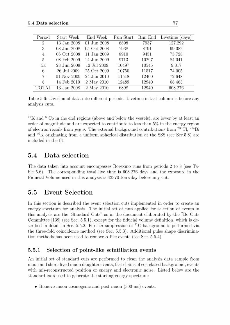
5.4 Data selection 77
Period Start Week End Week Run Start Run End Livetime (days)2 13 Jan 2008 01 Jun 2008 6898 7937 127.2923 08 Jun 2008 05 Oct 2008 7938 8791 99.0824 05 Oct 2008 11 Jan 2009 8910 9451 73.7285 08 Feb 2009 14 Jun 2009 9713 10297 84.0415a 28 Jun 2009 12 Jul 2009 10497 10545 9.0176 26 Jul 2009 25 Oct 2009 10750 11517 74.0057 01 Nov 2009 24 Jan 2010 11518 12400 72.6488 14 Feb 2010 2 May 2010 12489 12940 68.463
TOTAL 13 Jan 2008 2 May 2010 6898 12940 608.276
Table 5.6: Division of data into different periods. Livetime in last column is before anyanalysis cuts.
40K and 60Co in the end regions (above and below the vessels), are lower by at least anorder of magnitude and are expected to contribute to less than 5% in the energy regionof electron recoils from pep ν. The external background contributions from 208Tl, 214Biand 40K originating from a uniform spherical distribution at the SSS (see Sec.5.8) areincluded in the fit.
5.4 Data selectionThe data taken into account encompasses Borexino runs from periods 2 to 8 (see Ta-ble 5.6). The corresponding total live time is 608.276 days and the exposure in theFiducial Volume used in this analysis is 43370 ton×day before any cut.
5.5 Event SelectionIn this section is described the event selection cuts implemented in order to create anenergy spectrum for analysis. The initial set of cuts applied for selection of events inthis analysis are the “Standard Cuts” as in the document elaborated by the 7Be CutsCommittee [139] (see Sec. 5.5.1), except for the fiducial volume definition, which is de-scribed in detail in Sec. 5.5.2. Further suppression of 11C background is performed viathe three-fold coincidence method (see Sec. 5.5.3). Additional pulse shape discrimina-tion methods has been used to remove α-like events (see Sec. 5.5.4).
5.5.1 Selection of point-like scintillation events
An initial set of standard cuts are performed to clean the analysis data sample frommuon and short-lived muon daughter events, fast chains of correlated background, eventswith mis-reconstructed position or energy and electronic noise. Listed below are thestandard cuts used to generate the starting energy spectrum:
• Remove muon cosmogenic and post-muon (300 ms) events.

78Measurement of the pep and CNO solar neutrino interaction rates
in Borexino
• Remove zero cluster events.
• Remove sequence of fast coincidences (∆t <2 ms and ∆s < 1.5 m).
• Remove service triggers.
• Keep only events with a single cluster.
• Keep only events with cluster start time in the right position in the gate window.
• Remove events whose distribution of PMT hits is not uniform in space.
• Remove events outside the Fiducial Volume (FV).
• Remove electronic noise events.
The exact definition of these cuts is described in Sec. 2.3 of the Borexino internalnote [139]. Except for the last two cuts therein (15 and 16), all other cuts are imple-mented identically. These cuts remove less that < 0.3% of “good" events (details thePhD thesis [119]). The most relevant difference in the event selection with respect tothe 7Be ν analysis is a different fiducial volume definition, which is described in detail inSec. 5.5.2. The dead time introduced by these cuts in the context of the 7Be ν analysishas been evaluated in Sec. 2.5 of [119]. The largest loss of live time comes from theapplication of the 300 ms cut after muons, which has been measured to be 1.8% and hasbeen accounted for this analysis, decreasing the live time of the dataset to 598.14 days.The dead time due to the other cuts is < 1%, which is small compared to the system-atic uncertainties from the energy calibration and fit methods (Sec. 5.10.3), and can beneglected. Finally, the fast coincidence rate of events tagged as 214BiPo decays in theFV is used to estimate the 214Pb contamination in the final set of events and fix its ratein the fit.
5.5.2 Fiducial volume definition
The fiducial volume selected for this analysis was chosen so as to maximise the targetscintillator mass while minimising the effect of external background and variations inthe light collection efficiency.
5.5.2.1 External Background
As discussed in Sec. 5.3.3, there are two main sources of external background:
• background from the Stainless Steel Sphere (SSS), photomultiplier tubes, lightcones and other material connected to the SSS;
• background from the end-cap regions of the inner and outer nylon vessels.

5.5 Event Selection 79
x-5 -4 -3 -2 -1 0 1 2 3 4 5
z
-4
-2
0
2
4
1
10
210
z:x {sqrt(x^2+y^2+z^2) < 5 && abs(y) < 0.5 && m4_charge_noavg > 900 && m4_charge_noavg < 1500}
0
1
2
3
4
5
6
7
x-3 -2 -1 0 1 2 3
z
-3
-2
-1
0
1
2
3
z:x {sqrt(x^2+y^2+z^2) < 3 && abs(y) < 0.5 && m4_charge_noavg > 900 && m4_charge_noavg < 1500}
Figure 5.2: Spatial distribution of events with reconstructed position -1 m < y < 1 min the 900 - 1500 npe energy region, which is dominated by external γ-rays from 208Tland 214Bi. The positions are expressed in meters. Left panel: Events within the innervessel. Right panel: For r < 3 m.
To study the spatial distribution of γ-ray events from the SSS and other componentsat that radius, we plotted the reconstructed position of all events with charge between900 and 1500 number of photoelectrons (npe). This energy region is dominated by208Tl and 214Bi γ-ray interactions, with a smaller contribution (∼25%) from 10C and11C decays (see Fig. 5.16). The position of all events reconstructed within the InnerVessel (IV), in a 1 m thick slice ( -1 m < y < 1 m), is shown in Fig. 5.2. As can beseen, the number of events decreases as one moves radially away from the SSS towardsthe centre of the IV. The hot spots along the z-axis, at the top and bottom of the IVare due to the end-cap regions and will be discussed in detail below. A larger numberof events are seen in the top hemisphere, due to the fact that the deformed nylon vesselis closer to the SSS at the top than at the bottom. If the events are restricted tothose reconstructed within 3 m, the same radial cut used for the 7Be ν analysis [25],one can see (Fig. 5.2, right panel) that the z-dependence is no longer evident, and thebackground seems to increase uniformly with radius. We have found, by testing differentfiducial volumes, that the threefold coincidence cuts are most efficient at removing 11Cwithin a radius of 2.8 m. Therefore, the fiducial volume has been choosen to lie withina sphere of 2.8 m.
Due to their proximity to the scintillator, there is a large rate of background eventsoriginating from the end-cap regions of the inner and outer nylon vessel (see Fig. 5.2).The energy spectrum of the background from the end-cap regions is difficult to modeldue to the presence of multiple γ emissions and, like in the 7Be analysis [25], a fidu-cial volume cut along the z-axis was made to exclude events from those regions. Thebackground from the end-caps is most evident in the energy region between the 14C tailand the 210Po peak (120 - 145 npe). Fig. 5.3 shows the distribution of events in theentire IV and within 3 m. One can see that the top end-caps appear to be more activethan at the bottom, and that the events penetrate well within a 2.8 m radius. The tail

80Measurement of the pep and CNO solar neutrino interaction rates
in Borexino
x-4 -2 0 2 4
z
-4
-2
0
2
4
1
10
210
z:x {sqrt(x^2+y^2+z^2) < 5 && abs(y) < 0.5 && m4_charge_noavg > 120 && m4_charge_noavg < 145}
x-3 -2 -1 0 1 2 3
z
-3
-2
-1
0
1
2
3
0
2
4
6
8
10
12
14
16
18
20
22
z:x {sqrt(x^2+y^2+z^2) < 3 && abs(y) < 0.5 && m4_charge_noavg > 120 && m4_charge_noavg < 145}
Figure 5.3: Spatial distribution of events with reconstructed position -1 m < y < 1 m inthe energy region between the 14C tail and the 210Po peak (120 - 145 npe ), where theeffect of the background from the end caps is most evident. The positions are expressedin meters. Left panel: Events within the inner vessel. Right panel: For r < 3 m.
of events just under and above the top and bottom end-caps respectively are thoughtto be mis-reconstructed background events from the end-caps. A large fraction of thelight emitted by these events is occulted by the mechanical structure of the end-cap andcould cause events to be reconstructed radially inward. In order to safely exclude theseevents from the end-cap region, the fiducial volume must lie within 2.2 m > z > -2.4 m.
5.5.2.2 Light Collection Uniformity
The energy resolution, critical to obtaining a good spectral fit, depends strongly on theuniformity of the light collection within the fiducial volume. If one define the position-dependent light yield, relative to the value at the centre of the detector, as LY (~r),then the variance of the energy response function for a monoenergetic event with meancharge value Q is given by:
σ2(Q) = k ·Q+varFV (LY (~r))
mean2FV (LY (~r))
·Q2 , (5.2)
where the first term represents the intrinsic statistical variation of the scintillationprocess and meanFV (LY (~r)) and varFV (LY (~r)) are the mean and variance of the lightyield over the fiducial volume. In order to obtain a precise spectral fit, we require thatthe second term in Eq. 5.2 be less than 10% of the first over the energy range < 800 npe.One can evaluate the uniformity of the light collection by studying the peak positionof the 214Po source at different locations within the detector. By interpolating betweenthe source positions, we obtain a map of the light collection throughout the IV, asshown in Figure 5.4. It can be seen that the light collection is fairly uniform in the tophemisphere, but decreases as one moves downward due to the larger number of deadphotomultiplier tubes at the bottom. With the radial cut set at 2.8 m by the external

5.5 Event Selection 81
x [m]-4 -3 -2 -1 0 1 2 3 4
z [m]
-4
-3
-2
-1
0
1
2
3
4
0.8
0.85
0.9
0.95
1
1.05
1.1
Po source) distribution within IV214Conversion Probability (based on
Figure 5.4: Light collection efficiency within 3.5 m based on 214Po calibration sourcedata.
background from the SSS, and the upper z cut set at 2.2 m due to background fromthe top end-caps, we varied the lower z cut to maximise the volume while maintainingthe relative variation in light collection in uniformity. The optimal value for the lowerz cut was found to be -1.8 m.
5.5.2.3 Fiducial Volume Definition
Combining the above restrictions, we define the fiducial volume cut for this analysis asr < 2.8 m and 2.2 m > z > -1.8 m. The radial limit is determined by the externalbackground from the SSS sphere and the effectiveness of the three-fold coincidence cuts,the upper z cut is constrained by the background from the top end-cap regions, andthe lower z cut by the restriction on the light collection uniformity. The volume ofscintillator contained within this region is 81.26 m3 which corresponds to a fiducialmass of 71.30 tons.
5.5.3 Three-fold coincidence veto
The main background for the detection of pep ν in Borexino is 11C. The 11C nuclidesare produced by cosmogenic muons through a reaction resulting in the emission of freeneutrons in ∼ 95% of the cases [123]:
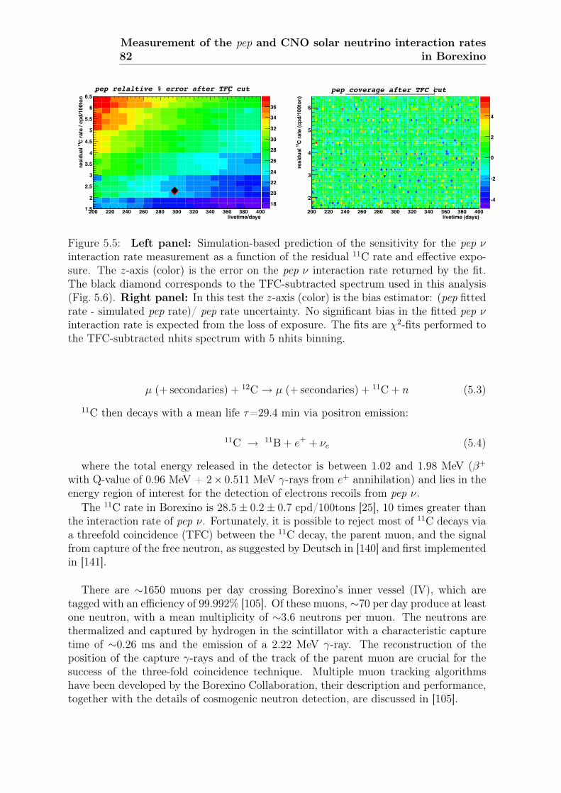
82Measurement of the pep and CNO solar neutrino interaction rates
in Borexino
livetime/days200 220 240 260 280 300 320 340 360 380 400
C ra
te /
cpd/
100t
on11
resi
dual
1.5
2
2.5
3
3.5
4
4.5
5
5.5
6
6.5
18
20
22
24
26
28
30
32
34
36
pep relaltive % error after TFC cut
livetime (days)200 220 240 260 280 300 320 340 360 380 400
C ra
te (c
pd/1
00to
n)11
resi
dual
2
3
4
5
6
-4
-2
0
2
4
pep coverage after TFC cut
Figure 5.5: Left panel: Simulation-based prediction of the sensitivity for the pep νinteraction rate measurement as a function of the residual 11C rate and effective expo-sure. The z-axis (color) is the error on the pep ν interaction rate returned by the fit.The black diamond corresponds to the TFC-subtracted spectrum used in this analysis(Fig. 5.6). Right panel: In this test the z-axis (color) is the bias estimator: (pep fittedrate - simulated pep rate)/ pep rate uncertainty. No significant bias in the fitted pep νinteraction rate is expected from the loss of exposure. The fits are χ2-fits performed tothe TFC-subtracted nhits spectrum with 5 nhits binning.
µ (+ secondaries) + 12C→ µ (+ secondaries) + 11C + n (5.3)
11C then decays with a mean life τ=29.4 min via positron emission:
11C → 11B + e+ + νe (5.4)
where the total energy released in the detector is between 1.02 and 1.98 MeV (β+
with Q-value of 0.96 MeV + 2× 0.511 MeV γ-rays from e+ annihilation) and lies in theenergy region of interest for the detection of electrons recoils from pep ν.
The 11C rate in Borexino is 28.5± 0.2± 0.7 cpd/100tons [25], 10 times greater thanthe interaction rate of pep ν. Fortunately, it is possible to reject most of 11C decays viaa threefold coincidence (TFC) between the 11C decay, the parent muon, and the signalfrom capture of the free neutron, as suggested by Deutsch in [140] and first implementedin [141].
There are ∼1650 muons per day crossing Borexino’s inner vessel (IV), which aretagged with an efficiency of 99.992% [105]. Of these muons, ∼70 per day produce at leastone neutron, with a mean multiplicity of ∼3.6 neutrons per muon. The neutrons arethermalized and captured by hydrogen in the scintillator with a characteristic capturetime of ∼0.26 ms and the emission of a 2.22 MeV γ-ray. The reconstruction of theposition of the capture γ-rays and of the track of the parent muon are crucial for thesuccess of the three-fold coincidence technique. Multiple muon tracking algorithmshave been developed by the Borexino Collaboration, their description and performance,together with the details of cosmogenic neutron detection, are discussed in [105].

5.5 Event Selection 83
The threefold coincidence algorithm vetoes space-time regions of the detector aftermuon and neutron coincidences in order to exclude the subsequent 11C decays. Theguiding principle for the determination of the most appropriate parameters is the searchfor the best compromise between 11C rejection and preservation of residual exposureafter the veto cuts. We have applied different veto configurations on the data, resultingin different residual 11C rates and effective residual exposures. From an analysis onsimulated data samples (Fig. 5.5), we estimated which configuration leads to the smallestexpected uncertainty in the pep ν interaction rate.
The evaluation of the effective residual exposure after all veto cuts, many of whichoverlap in time and space, has been performed using two independent ways. In the firstway, we assumed that 210Po, which rate is high in Borexino and which events can beeasily selected by means of pulse-shape and energy cuts, is uncorrelated with the TFCcuts and, therefore, the number of counts that survive the vetoes should be proportionalto the residual exposure. In the second way, we developed a simulation feeding eventsuniformly in space and time to the veto cuts. The residual exposure is computed fromthe fraction of the simulated events that survive the vetoes. The residual exposurescalculated by these two ways agrees to much better than 1%. An initial evaluation ofthe residual 11C after the application of the TFC is done by checking the fraction ofevents that survive the cuts in an energy interval where mostly 11C is expected, namelybetween 530 and 610 nhits. A small component of external background contributes tocounts in this energy region and cannot be easily estimated, therefore 11C suppressioncan actually be better than quoted.
The TFC procedure can be summarised as follows:
• A 2 hours blackout is applied at the beginning of each DST, rejecting any event inthe entire detector. This is needed since the current processing of DSTs is done inparallel, and no information regarding muon and neutron coincidences in carriedover between DSTs.
• Additional blackouts have been applied at the beginning of each run, since muonand neutron coincidences can be lost in the interval between runs. The veto timein minutes is obtained by 10 + 60 (1− exp (−3∆t/τ)), where ∆t is the dead-timeinterval between subsequent runs in minutes.
• For high multiplicity events a blackout of 2 hours is applied.
• When the reconstructed neutron position is not reliable, due to DAQ saturationand/or to a large fraction of noise hits, we apply a cylindrical veto along theparent muon track with a radius of 80 cm for a time span of 2 hours.
• If neutron clusters in a muon gate are found more than 2 µs after the muon, thenthe cylindrical veto along the muon track described above is applied.
• A cylindrical veto is also applied around muon tracks in events with nhits > 1000after which at least one neutron is found.
• If a neutron is found and its position is considered reliable, we exclude any eventless than 1 m away from it for 2 hours. Moreover, the neutron projection on the
84Measurement of the pep and CNO solar neutrino interaction rates
in Borexino
parent muon track is calculated and another 2 hours, 1 m spherical veto is appliedaround this position.
The application of the algorithm on the selected data results in > 89.4% 11C rejectionwith a residual exposure of 48.5%. Fig. 5.6 shows the starting and the final spectrumfollowing the stage of 11C reduction performed with the three-fold coincidence veto.The resulting exposure of the TFC-subtracted spectrum is 20409 days × tons, while forthe spectrum of the TFC-tagged events it is 23522 days × tons.
It is important to remark that overall acceptance and leakage of the TFC cuts arenot expected to introduce any bias in the final result (see Sec. 5.10), as long as theydo not cause a spectral distortion in the energy spectrum. By the way the TFC vetois defined, its overall acceptance and leakage should be completely uncorrelated fromthe visible energy of the event. An increase in the efficiency of the TFC would primaryresult in a final spectrum with a reduced 11C component. Vice versa, should the neutronidentification fail in a fraction of the events, this would cause an increase in the 11Ccomponent or a reduction of the overall unvetoed exposure. In both cases no distortionof the energy spectrum, which could potentially result is a bias in the final result, isexpected.
The TFC veto can also be used to tag high-purity sample of 11C events. Thesesamples has been used for several purposes, like understanding the dependence of thereconstructed energy of the event with respect the position and tune the light yield of theMonte Carlo simulation, studying the pulse shape of the 11C events in order to identifythe o-Ps formation (see Sec. 5.7.2) and develop pulse shape variables to discriminatebetween β+ and β− events (see Sec. 5.7.3).
5.5.4 Statistical subtraction of α-like events
α-like events are removed from the final energy spectrum with the method of statisticalsubtraction. For each energy bin, the distribution of the Gatti variable (see Sec. 3.4.2)is fitted using two reference distributions, one representing the β population, the secondone, the α population. For each energy bin we fit and separate the two components,thus computing the relative amount of α ad β events. In this way, the contributionsfrom 210Po and other α decays are statistically removed from the energy spectrum. Thedetailed description of the method, its implementation, efficiency, systematic effects,biases, and other related issues are discussed in detail in the PhD thesis [118] and [119].Fig. 5.7 shows the final spectrum before and after this procedure.
5.6 Energy variables
Within the Borexino analysis framework (MOE-Echidna), several energy variables areavailable, each with a slightly different method of estimating the energy of a given event.The definition of the energy variables used in this analysis are given below. Additionalinformation on the energy variables, their implementation, biases, simulation, analyticalcomputation, and other related issues can be found in the PhD thesis [118] and [119].

5.6 Energy variables 85
npe200 400 600 800 1000 1200 1400
Eve
nts
/ (20
409
days
x to
ns x
5 p
.e.)
1
10
210
310
410 After TFC veto
C subtraction11No
Energy spectrum in FV
Figure 5.6: Normalized Borexino energy spectrum before and after application oftechniques for 11C removal. The black line shows the untreated spectrum, with∼28 cpd/100 tons of 11C. The blue line shows the resulting spectrum after apply-ing the three-fold coincidence veto described in Sec. 5.5.3, which decreases the 11C rateto ∼2.5 cpd/100 tons with a 51.5% loss of exposure.
5.6.1 Echidna nhits
This is the number of PMT hits in the long, fixed length (1500 ns), cluster window.After each PMT hit, there is a hardware dead time of 140 ns in the hit channel. Anadditional software dead time of 40 ns is applied, in order to not include spurious hitsdue to re-triggering. The total number of hits is then scaled by 2000/(No. of PMTswith valid timing readout).
5.6.2 MOE npe_noavg_corrected
This is the total, summed photoelectron charge of every “valid-charge" hit, includingthose from re-triggered channels, within the variable-length MOE cluster. Single channeldead times are the same as those for Echidna nhits. The expected number of dark noisehits in the cluster is subtracted. The total charge is then scaled by 2000/(No. of PMTswith valid charge readout).

86Measurement of the pep and CNO solar neutrino interaction rates
in Borexino
npe200 400 600 800 1000 1200 1400
Eve
nts
/ (20
409
days
x to
ns x
5 p
.e.)
1
10
210
310
410 subtractionαNo
subtractionαAfter
Energy spectrum in FV
Figure 5.7: Normalized Borexino energy spectrum before and after statistical subtrac-tion of α-like events. The red line shows the energy spectrum after applying the three-fold coincidence veto described in Sec. 5.5.3 and before α subtraction. The blue lineshows the resulting spectrum after applying the α statistical subtraction technique re-ferred in Sec. 5.5.4.
5.7 β+/β− pulse-shape discrimination
The 11C surviving the TFC veto is still a significant background for the pep ν andCNO νs interaction rate measurement. We developed and adopted novel data analysistechniques, exploiting the pulse shape differences between e− and e+ interactions inorganic liquid scintillators, in order to discriminate 11C β+ decays from neutrino-inducede− recoils and β− decays.
5.7.1 Principles of β+/β− pulse-shape discrimination in liquidscintillators
The profile of the reconstructed emission times for scintillation photons produced by apositron that deposits its energy in the target should be different than those from anelectron. After the positron deposits its kinetic energy, it annihilates with electrons inthe scintillator emitting two back-to-back γ-rays. The time lag in the physical processof positron annihilation, as well as the fact that the energy is deposited by multipleparticles, leads to differences in the reconstructed emission time of the detected photons
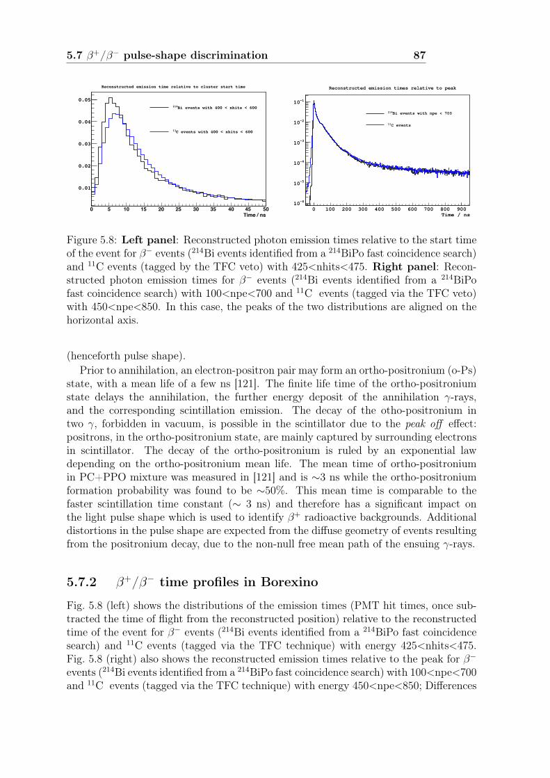
5.7 β+/β− pulse-shape discrimination 87
Time / ns0 5 10 15 20 25 30 35 40 45 50
0.01
0.02
0.03
0.04
0.05Bi events with 400 < nhits < 600214
C events with 400 < nhits < 60011
Reconstructed emission time relative to cluster start time
Time / ns0 100 200 300 400 500 600 700 800 900
-610
-510
-410
-310
-210
-110
Bi events with npe < 700214
C events11
Reconstructed emission times relative to peak
Figure 5.8: Left panel: Reconstructed photon emission times relative to the start timeof the event for β− events (214Bi events identified from a 214BiPo fast coincidence search)and 11C events (tagged by the TFC veto) with 425<nhits<475. Right panel: Recon-structed photon emission times for β− events (214Bi events identified from a 214BiPofast coincidence search) with 100<npe<700 and 11C events (tagged via the TFC veto)with 450<npe<850. In this case, the peaks of the two distributions are aligned on thehorizontal axis.
(henceforth pulse shape).Prior to annihilation, an electron-positron pair may form an ortho-positronium (o-Ps)
state, with a mean life of a few ns [121]. The finite life time of the ortho-positroniumstate delays the annihilation, the further energy deposit of the annihilation γ-rays,and the corresponding scintillation emission. The decay of the otho-positronium intwo γ, forbidden in vacuum, is possible in the scintillator due to the peak off effect:positrons, in the ortho-positronium state, are mainly captured by surrounding electronsin scintillator. The decay of the ortho-positronium is ruled by an exponential lawdepending on the ortho-positronium mean life. The mean time of ortho-positroniumin PC+PPO mixture was measured in [121] and is ∼3 ns while the ortho-positroniumformation probability was found to be ∼50%. This mean time is comparable to thefaster scintillation time constant (∼ 3 ns) and therefore has a significant impact onthe light pulse shape which is used to identify β+ radioactive backgrounds. Additionaldistortions in the pulse shape are expected from the diffuse geometry of events resultingfrom the positronium decay, due to the non-null free mean path of the ensuing γ-rays.
5.7.2 β+/β− time profiles in Borexino
Fig. 5.8 (left) shows the distributions of the emission times (PMT hit times, once sub-tracted the time of flight from the reconstructed position) relative to the reconstructedtime of the event for β− events (214Bi events identified from a 214BiPo fast coincidencesearch) and 11C events (tagged via the TFC technique) with energy 425<nhits<475.Fig. 5.8 (right) also shows the reconstructed emission times relative to the peak for β−events (214Bi events identified from a 214BiPo fast coincidence search) with 100<npe<700and 11C events (tagged via the TFC technique) with energy 450<npe<850; Differences

88Measurement of the pep and CNO solar neutrino interaction rates
in Borexino
may be observed in both the peak time and the rise and decay times of the distributions.We believe that these differences are mostly due to the delay induced by the o-Ps life-
time: when the β+ undergoes o-Ps formation, the scintillation light produced by the twoannihilation γ-rays is delayed with respect to the prompt scintillation light producedby the kinetic energy loss of the β+. The ratio R between the annihilation energy andthe kinetic energy T of the β+ is not constant with respect to the energy of the β+:
R =2mec
2
T, (5.5)
where mec2 is the rest energy of electrons and positrons, and therefore 2me2
c is theenergy of the 2 annihilation γ-rays. The fraction of the delayed hits induced by theo-Ps decay, respect to the total number of hits, is then lower when the kinetic energy ofthe β+ is higher. The difference between β+ and β− reconstructed emission time, as wellas the discrimination power of any pulse-shape based method, is then energy-dependent,and it is lower as the energy of the β+ event increases.
In order to detect and quantify this effect in Borexino data, as well as to developpulse shape variables to discriminate β+ and β− events, we have developed a specialMonte Carlo event generator to simulate o-Ps formation and yield the corrected pulseshape (see Sec. 4.2.1.3). According to the input formation probability and lifetime, thecode generates positron annihilations and positronium decays. The delay of the γ-raysfollows an exponential law depending on the o-Ps mean life.
An evidence that the o-Ps is generated in a fraction of β+ events in the Borexinodata sample comes from the comparison of the pulse shape of the reconstructed photonemission times, in a pure sample of β+ events, with respect to simulations of o-Ps pulseshape. The sample of β+ events is provided thanks to the TFC veto, that allows high-purity sample of 11C decays. We have compared the pulse shape of these events indata with the pulse shape of simulated 11C decays with different o-Ps mean life andformation probability. This comparison rejected the hypothesis of no o-Ps formationin the data, and evidenced o-Ps formation with mean life and probability in agreementwith the laboratory measurement in [121]. The comparison between the reconstructedemission times for 11C events between real data and a simulated data sample is shownin Fig. 5.9.
5.7.3 Boosted-decision-tree analysis
We have developed a method of particle identification, based on pulse-shape discrimina-tion, for 11C events. The method utilises the Boosted Decision Tree (BDT) algorithm ofthe Toolkit for MultiVariate Analysis (TMVA) [142], included in the standard ROOTdistribution [143]. This technique requires carefully chosen training sets of data forsignal and background to build a weighted (boosted) decision tree, which optimises thecuts on a user-defined set of variables, for best identifying the signal against the back-ground. The trained method returns a number for each event. Test event sets define adistribution of such number which the user can then use to discriminate between signaland background.
To train the BDT, we selected as the signal sample the low energy 214BiPo events(450<npe<900), which are a relatively clean β− sample (∼95% of events in 450–700

5.7 β+/β− pulse-shape discrimination 89
Time / ns10 20 30 40 50 60
0.005
0.01
0.015
0.02
0.025
0.03
0.035
0.04
0.045C Reconstructed emission time (410 < nhits < 670)11
C 11DATA
C - no Ps formation11MC
0.031± = 3.1 ns): 0.53 τC - oPs (11MC
Best Fit
Figure 5.9: Reconstructed photon emission times for 11C decays in Borexino data (blackline). The 11C events are tagged with the TFC veto. The data pulse shape is fittedwith the sum of two Monte Carlo simulated pulse shapes of 11C decays (red line), onewith 100% o-Ps formation (blue line) and one without o-Ps formation (green line). Inthis particular trial the o-Ps mean life is 3.1 ns. The weight of the pulse shape witho-Ps formation represents the o-Ps probability formation, which is a free parameter inthe fit. The fitted o-Ps formation probability (53%) and the mean life (∼ 3 ns) of thistrial is in agreement with the laboratory measurement in [121].
npe range are pure β− decays, while ∼60% of those in the range 700–900 have someγ-ray contribution). We selected as the background sample those events tagged bythe three-fold coincidence with energy 450<npe<900, which should be an almost pure(> 98%) 11C sample. All of the events considered have reconstructed positions withr <3 m and 2.2 m > z > -1.8 m, which are the z-cuts used to define the FV (Sec. 5.5.2).The training and test samples are the same size, with 1400 signal (β−) events and 3175background (β+) events. The cluster variables considered by the BDT analysis are:
• The Gatti parameter (see Sec. 3.4.2) computed using as reference the 214Bi and11C time profiles from real data, with reconstructed emission time relative to thepeak.
• The Gatti parameter computed using as reference the 214Bi and 11C time profilesfrom real data, with reconstructed emission time relative to the cluster start.
• The Gatti parameter computed using as reference the 214Bi and o-Ps (Monte

90Measurement of the pep and CNO solar neutrino interaction rates
in Borexino
Carlo-generated) time profiles, with reconstructed emission time relative to thecluster start.
• The Gatti parameter computed using as reference the Monte Carlo-generated11C time profiles with and without o-Ps formation, with reconstructed emissiontime relative to the cluster start.
• The Gatti parameter computed using as reference the 214Bi and 214Po time profilesfrom data.
• The Kolmogorov-Smirnov probabilities between the emission time distribution ofthe event and the 214Bi or 214Po reference time profiles.
• The reconstructed emission time, relative to the peak of the time distribution, ofthe earliest hit in the cluster.
• The peak of the emission time distribution relative to the reconstructed time ofthe event.
• The first four moments of the emission time distribution (i.e. mean, rms, skewnessand kurtosis) for hits up to 1.1 µs after the cluster start.
• Ten tail-to-total (see Sec. 3.4.2) variables that are the fraction of the hits in thecluster after particular times (35, 70, 105, 140, 175, 210, 245, 280, 315 and 350 ns)relative to the peak of the distribution.
• The first four Legendre polynomials, averaged over all combinations, of the anglebetween any two hit PMTs relative to the reconstructed position of the event.
• The uncertainties in the reconstructed position along an axis (x, y, z, as returnedby the fitter) divided by the mean of the other two uncertainties.
• The ratio (for all axes) of the reconstructed position of the event obtained from thetime-of-flight subtraction algorithm to the charge-weighted average of the PMTpositions in the event.
The final output variable of the BDT algorithm (the PS-BDT parameter) and thecorresponding distribution of the test samples is shown in Fig. 5.10.
As the training and test samples are statistically independent, the probability distri-bution functions (PDFs) from which the PS-BDT parameter distributions for the testsamples are drawn should be the same as those for the final candidates, as long asthey belong to the same population of events. The probability of the 11C decay to beselected by a TFC veto should be independent on the details of the decay, includingthe energy of the positron emitted and the probability that it forms ortho-positronium,and, therefore, the test sample for the β+ should have the same distribution in energyand all variables included in the computation of the PS-BDT parameter as the 11Cdecays in the final data sample. The efficiency in the TFC tagging has been observedto be spatially uniform up to 2.8 m from the centre of the detector (Sec. 5.5.3). Forthe training candidate sample of the PS-BDT parameter we have included events up

5.7 β+/β− pulse-shape discrimination 91
PS-BDT Parameter-0.8 -0.6 -0.4 -0.2 0 0.2
-310
-210
-110-β+β
PS-BDT distributions for test samples
Figure 5.10: Distributions of the PS-BDT parameter for the test samples of β− (greenline) and β+ (blue line) events. β− are low energy (< 900 npe) 214Bi events selectedfrom fast 214BiPo coincidences. β+ events are 11C events tagged via the TFC tech-nique described in Sec. 5.5.3. The training was performed using ROOT’s Toolkit forMultiVariate Analysis and the pulse shape cluster variables listed in Sec. 5.7.3.
to 3 m but, as we observed no noticeable dependence of the PS-BDT parameter onreconstructed radial position and, we do not expect any differences between the testsample distribution and that of the 11C decays in the final candidates sample.
The differences between the test sample and the β−events in the final candidates arelarger. Not only is the test sample itself composed of some events that have some γ-ray contribution, but in the final candidates there should also be some external γ-rays.The profile is similar in both cases, with γ-ray contributions increasing towards higherenergies, yet the relative composition as a function of energy has not been shown tobe identical. We have argued that the largest difference between the pulse shape of β+
and β− events is due to the delayed γ-rays from the formation of ortho-positronium,but we have also acknowledged that the diffuse nature of the energy deposits in the β+
decay, which may be similar to those from single γ-rays, could also lead to pulse-shapedifferences (Sec. 5.7.1). As mentioned earlier, the γ-ray contribution to the 214Bi samplestarts at ∼700 npe and therefore, if the increase in the γ-ray content has an effect in thePS-BDT parameter, we may see a change in the distribution after this point. Fig. 5.11(right) shows the energy dependence of the mean value of the PS-BDT parameter forboth 11C and 214Bi test samples. As may be observed, there is indeed an increase in

92Measurement of the pep and CNO solar neutrino interaction rates
in Borexino
npe450 500 550 600 650 700 750 800 850 900
Normalized counts
0
0.05
0.1
0.15
0.2
0.25
0.3
Bi214
C11
Energy spectra of test samples
npe450 500 550 600 650 700 750 800 850 900
PS-BDT Parameter
-0.2
-0.15
-0.1
-0.05
0
0.05
0.1
PS-BDT dependence on energy
Bi214
C11
Figure 5.11: Left panel: Energy spectrum for the events in the 11C (β+) and lowenergy 214Bi (β−) test samples. Right panel: Mean value for the PS-BDT distributionin the corresponding npe bin. For both test samples, the PS-BDT value increases athigher energies. The energy dependence of the parameter will not lead to any differencesbetween the PS-BDT distributions of a test sub-sample and the corresponding events inthe final candidates sample, as long as the energy spectrum does not differ considerablyin the energy range of the events in the distribution.
the PS-BDT mean at higher energies, but this effect is present in both test samples,which suggests that it is due to an overall dependence of the PS-BDT parameter on theenergy and not necessarily correlated with the increase in the γ-ray contribution in the214Bi sample. The energy dependence itself should not be a problem for our analysis, aslong as the energy bins for the PS-BDT distributions that we consider are small enoughsuch that neither the PS-BDT mean values nor the energy spectra for the test and finalsamples differ considerably throughout them. In Sec. 5.10.3.6 we perform an evaluationof the systematic uncertainty induced by these issues.
Additionally, the spatial distribution of the events in the 214Bi sample is not the sameas the β− events in the final candidates. The 214Bi events selected are decay productsof 222Rn, which has been mostly introduced into the detector during operations (fromthe top) or has been emanated by the nylon vessels, leading to a non-uniform spatialdistribution. Furthermore, some of the events in the final candidates considered β− areexternal γ-rays, whose position is preferentially reconstructed towards the edge of theFV. Fig. 5.12 (right) show the relationship between the 214Bi PS-BDT parameter andthe reconstructed z event coordinate. Fits to the mean values of the PS-BDT distribu-tions as a function of both r and z are consistent with the PS-BDT parameter beingindependent on position (p-values of 0.5 when fit to a constant), suggesting that no con-siderable differences are introduced in the PS-BDT distributions due to the differencesin the spatial distribution of the test and final candidates samples.
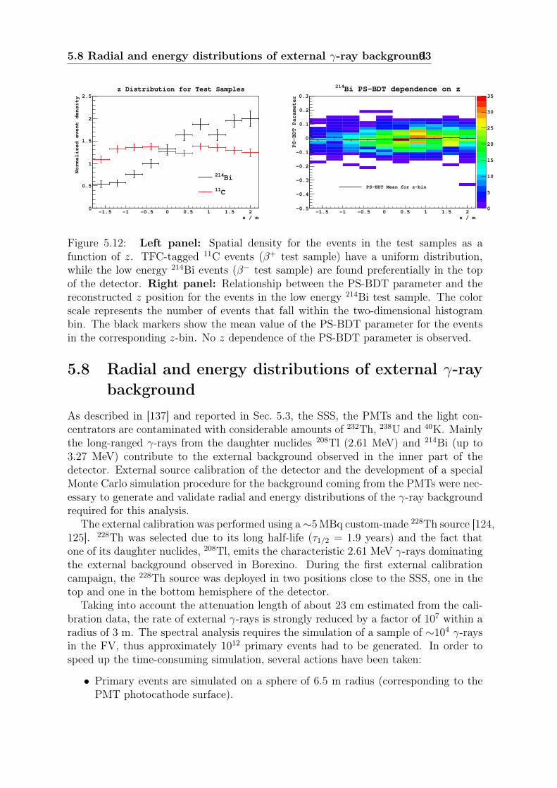
5.8 Radial and energy distributions of external γ-ray background93
z / m-1.5 -1 -0.5 0 0.5 1 1.5 2
Normalized event density
0
0.5
1
1.5
2
2.5
Bi214
C11
z Distribution for Test Samples
z / m-1.5 -1 -0.5 0 0.5 1 1.5 2
PS-BDT Parameter
-0.5
-0.4
-0.3
-0.2
-0.1
0
0.1
0.2
0.3
0
5
10
15
20
25
30
35Bi PS-BDT dependence on z214
PS-BDT Mean for z-bin
Figure 5.12: Left panel: Spatial density for the events in the test samples as afunction of z. TFC-tagged 11C events (β+ test sample) have a uniform distribution,while the low energy 214Bi events (β− test sample) are found preferentially in the topof the detector. Right panel: Relationship between the PS-BDT parameter and thereconstructed z position for the events in the low energy 214Bi test sample. The colorscale represents the number of events that fall within the two-dimensional histogrambin. The black markers show the mean value of the PS-BDT parameter for the eventsin the corresponding z-bin. No z dependence of the PS-BDT parameter is observed.
5.8 Radial and energy distributions of external γ-raybackground
As described in [137] and reported in Sec. 5.3, the SSS, the PMTs and the light con-centrators are contaminated with considerable amounts of 232Th, 238U and 40K. Mainlythe long-ranged γ-rays from the daughter nuclides 208Tl (2.61 MeV) and 214Bi (up to3.27 MeV) contribute to the external background observed in the inner part of thedetector. External source calibration of the detector and the development of a specialMonte Carlo simulation procedure for the background coming from the PMTs were nec-essary to generate and validate radial and energy distributions of the γ-ray backgroundrequired for this analysis.
The external calibration was performed using a∼5MBq custom-made 228Th source [124,125]. 228Th was selected due to its long half-life (τ1/2 = 1.9 years) and the fact thatone of its daughter nuclides, 208Tl, emits the characteristic 2.61 MeV γ-rays dominatingthe external background observed in Borexino. During the first external calibrationcampaign, the 228Th source was deployed in two positions close to the SSS, one in thetop and one in the bottom hemisphere of the detector.
Taking into account the attenuation length of about 23 cm estimated from the cali-bration data, the rate of external γ-rays is strongly reduced by a factor of 107 within aradius of 3 m. The spectral analysis requires the simulation of a sample of ∼104 γ-raysin the FV, thus approximately 1012 primary events had to be generated. In order tospeed up the time-consuming simulation, several actions have been taken:
• Primary events are simulated on a sphere of 6.5 m radius (corresponding to thePMT photocathode surface).
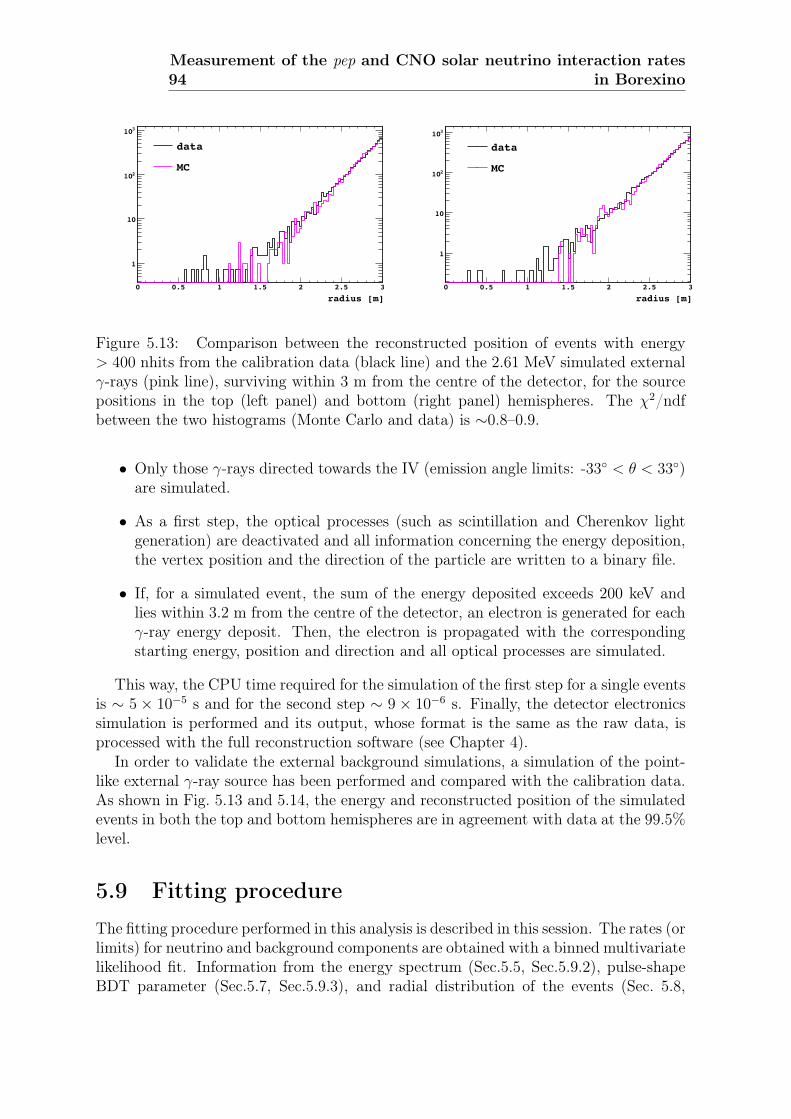
94Measurement of the pep and CNO solar neutrino interaction rates
in Borexino
radius [m]0 0.5 1 1.5 2 2.5 3
1
10
210
310
data
MC
radius [m]0 0.5 1 1.5 2 2.5 3
1
10
210
310
data
MC
Figure 5.13: Comparison between the reconstructed position of events with energy> 400 nhits from the calibration data (black line) and the 2.61 MeV simulated externalγ-rays (pink line), surviving within 3 m from the centre of the detector, for the sourcepositions in the top (left panel) and bottom (right panel) hemispheres. The χ2/ndfbetween the two histograms (Monte Carlo and data) is ∼0.8–0.9.
• Only those γ-rays directed towards the IV (emission angle limits: -33◦ < θ < 33◦)are simulated.
• As a first step, the optical processes (such as scintillation and Cherenkov lightgeneration) are deactivated and all information concerning the energy deposition,the vertex position and the direction of the particle are written to a binary file.
• If, for a simulated event, the sum of the energy deposited exceeds 200 keV andlies within 3.2 m from the centre of the detector, an electron is generated for eachγ-ray energy deposit. Then, the electron is propagated with the correspondingstarting energy, position and direction and all optical processes are simulated.
This way, the CPU time required for the simulation of the first step for a single eventsis ∼ 5 × 10⁻⁵ s and for the second step ∼ 9 × 10⁻⁶ s. Finally, the detector electronicssimulation is performed and its output, whose format is the same as the raw data, isprocessed with the full reconstruction software (see Chapter 4).
In order to validate the external background simulations, a simulation of the point-like external γ-ray source has been performed and compared with the calibration data.As shown in Fig. 5.13 and 5.14, the energy and reconstructed position of the simulatedevents in both the top and bottom hemispheres are in agreement with data at the 99.5%level.
5.9 Fitting procedure
The fitting procedure performed in this analysis is described in this session. The rates (orlimits) for neutrino and background components are obtained with a binned multivariatelikelihood fit. Information from the energy spectrum (Sec.5.5, Sec.5.9.2), pulse-shapeBDT parameter (Sec.5.7, Sec.5.9.3), and radial distribution of the events (Sec. 5.8,

5.9 Fitting procedure 95
normalized nhits200 300 400 500 600 700 800 900 1000 1100
1
10
210
data
MC
normalized nhits200 300 400 500 600 700 800 900 1000 1100
10
210
data
MC
Figure 5.14: Comparison between the reconstructed nhits for events from the calibra-tion data (black line) and the 2.61 MeV simulated external γ-rays (pink line), survivingwithin 3 m from the centre of the detector, for the source positions in the top (leftpanel) and bottom(right panel) hemispheres. The χ2/ndf between the two histograms(Monte Carlo and data) is ∼ 1.2.
Sec. 5.9.4) are included in the likelihood (Sec. 5.9.1) to maximise. The 11C subtractedenergy spectrum (Sec 5.5.3) and its complementary (TFC-vetoed) spectrum are fittedsimultaneously. The fit method has been validated using data-like samples of knowninput composition (Sec. 5.10.2).
5.9.1 Multi-dimensional fitting strategy
The method of maximum likelihood (see Sec. 33.1.2 in [2]) is used in the pep ν analysisto fit the data. The likelihood was chosen as test statistic for two reasons:
• the small number of entries in some of the high energy bins of our final energyspectrum;
• the possibility to extend the likelihood in a multi-dimensional approach, in orderto include the β+ / β− pulse-shape BDT parameter (Sec. 5.7) and the radialdistribution of the events (Sec. 5.8) in the likelihood to maximise.
For a one-dimensional fit, one would compute the Poisson likelihood, L, of a hypoth-esis (i.e. the likelihood that the data fits a test spectrum with a set of parameters ~θ)as
L(~θ) =n∏i=1
λi(~θ)kie−λi(
~θ)
ki!(5.6)
where the product is over all bins and n is the total number of bins. λi(~θ) is theexpected number of entries in the ith bin given the fit parameters (~θ) and ki is thenumber of entries in the bin. As an example, ki could be the number of entries in aparticular energy bin, and λ(~θ) the expected number of entries in that bin given therates of each species described by the array of parameter θ.

96Measurement of the pep and CNO solar neutrino interaction rates
in Borexino
For the pep ν analysis, in order to constrain the impact of the background due to 11Cdecays and the external γ-rays, the likelihood is extended to other variables, namely,the pulse-shape BDT parameter (Sec. 5.7) and the radial distribution (Sec. 5.8) of theevents. The probability density functions (PDFs) of some of these variables are producedfrom data (e.g. the pulse-shape PDF for β− is taken from tagged 214BiPo events) andwe do not have neither very high statistics, nor an analytical model to produce precisemulti-dimensional PDFs. Therefore, the events are projected and integrated over anenergy range larger than the energy spectrum binning, into one-dimensional histogramsof the other variables, and the corresponding likelihood is computed. In this case though,a correlation between the number of counts in the different histograms is introduced,as events that are in the energy spectrum will also be entries in the projections. Tohandle this issue, the PDFs of the hypothesis are normalized to the total number ofentries in the projected data histograms. Consequently, the likelihood computed for theprojections is defined as:
Lp(~θ) =m∏j=1
aλj(~θ)kje−aλj(
~θ)
kj!(5.7)
N = am∑j=1
λj(~θ) (5.8)
where N is the total number of entries in the projected histogram and a is a scalingfactor set to satisfy Eq. 5.8. Here λj(~θ) represents the expected bin content of theprojected histogram in the corresponding other variable, and kj is the actual number ofentries in that bin. The scaling does not affect the values of λ(~θ) at the maximum like-lihood but the uncertainties given by likelihood ratio tests may not be underestimated,as it is the case when the scaling is not done. Even though we have not demonstratedthat this procedure is mathematically sound, in Sec. 5.10.2 we perform MonteCarlo testswith data-like samples to show that the statistical interpretation of likelihood ratio testsholds for the computed total likelihood.
The total likelihood to maximise is then
LT (~θ) =mE∏i=1
L(~θ)×mp∏j=1
Lp(~θ) (5.9)
where L(~θ) and Lp(~θ) are defined in Eq. 5.6 and 5.7, respectively. The first productis over the mE independent energy spectra (e.g. those of the TFC-tagged and TFC-subtracted events, see Sec. 5.9.2) and the second is the product over all mp projectionsto other dimensions (e.g. radial distribution and PS-BDT parameter space) of regionsof one of the energy spectra. This definition has been implemented into the fitting code,which pass − lnLT (~θ) to MINUIT as the test statistic to be minimised.
As we are using PDFs from data with limited statistics for the fit to the PS-BDTparameter space, we have had to introduce a correction to handle the possibility ofthere being an event in a bin for which there are no events in the corresponding fittingPDF, not because the true λi is zero, but because of the limited statistics. This effect isreduced greatly since a “smoothing” is applied to the fitting PDFs (Sec. 5.9.3), increasing

5.9 Fitting procedure 97
the statistics significantly and filling up empty bins. The detailed explanation of themodification will be omitted here as it comes from a redefinition of the likelihood forwhich its total value is almost identical to the one obtained from Eq. 5.9, except for thecase where λi = 0 and ki > 0. In such case, the likelihood for the bin becomes
Li =(
N
NPDF + n
)ki(5.10)
where n is the number of bins in the histogram and N and NPDF are the entries in theprojected histogram and the fitting PDF, respectively. The probability computed bythis method, albeit small as generally NPDF � N , is non-zero and, therefore, can behandled appropriately by the fitter.
For this analysis, we have not made any particular corrections to the likelihoodfor the bins over which the bin contents (and their corresponding uncertainties) havebeen changed by the statistical α subtraction procedure (Sec. 5.5.4). Generally, theuncertainties remain unchanged except for the region of the 210Po peak (150–250 npe).For example, in the case of the npe spectrum, out of 146 bins, only 18 had an increasein uncertainty > 5% and only 5 had an increase > 15%. Not considering this increasein the uncertainty will not affect the best fit value (i.e. the values of λ(~θ) for which themaximum likelihood is found), but may have a small effect in the uncertainty returnedby the fit for species determined by this region of the spectrum, namely 7Be, 85Kr and210Bi.
5.9.2 Fit to the energy spectra
5.9.2.1 Subtracted and complementary energy spectrum fit
We have applied a binned likelihood fit to the energy spectra obtained from the eventselection outlined in Sec. 5.5. Both the TFC-subtracted spectrum and its complemen-tary spectrum are fitted simultaneously, keeping the rates of most species as commonparameters (see Table 5.7). The only species whose rates are different parameters in thetwo spectra are 11C, 10C and 6He. The 11C rate is indeed suppressed by the TFC, as itis correlated with neutron production (Sec. 5.5.3). 10C and 6He are also cosmogenic innature and their production may also be correlated with neutrons, therefore their ratesare kept independent in the two spectra.
5.9.2.2 Input energy spectra
In order to check for consistency within our assumptions and to get an evaluation of thesystematics involved with the energy detector response function, we use two differentenergy variables to fit the energy spectrum. The energy variables used are nhits andm4charge_noavg (npe), whose descriptions are in Sec. 5.6. The energy spectrum PDFsused to fit the nhits and m4charge_noavg (npe) spectra have been produced with inde-pendent methods: the PDFs for nhits have been obtained with the full Monte Carlo sim-ulation of the Borexino detector (see Chapter 4), while the PDFs for m4charge_noavg(npe) are based on an analytical model of the detector response.
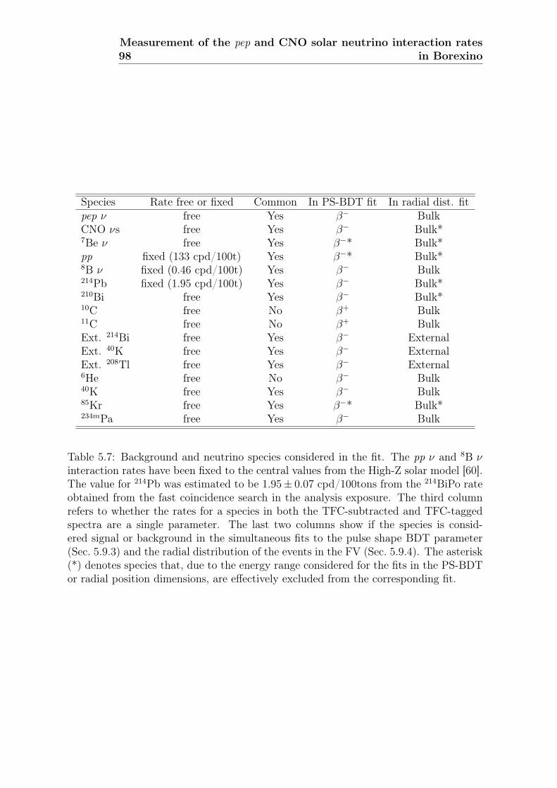
98Measurement of the pep and CNO solar neutrino interaction rates
in Borexino
Species Rate free or fixed Common In PS-BDT fit In radial dist. fitpep ν free Yes β− BulkCNO νs free Yes β− Bulk*7Be ν free Yes β−* Bulk*pp fixed (133 cpd/100t) Yes β−* Bulk*8B ν fixed (0.46 cpd/100t) Yes β− Bulk214Pb fixed (1.95 cpd/100t) Yes β− Bulk*210Bi free Yes β− Bulk*10C free No β+ Bulk11C free No β+ BulkExt. 214Bi free Yes β− ExternalExt. 40K free Yes β− ExternalExt. 208Tl free Yes β− External6He free No β− Bulk40K free Yes β− Bulk85Kr free Yes β−* Bulk*234mPa free Yes β− Bulk
Table 5.7: Background and neutrino species considered in the fit. The pp ν and 8B νinteraction rates have been fixed to the central values from the High-Z solar model [60].The value for 214Pb was estimated to be 1.95± 0.07 cpd/100tons from the 214BiPo rateobtained from the fast coincidence search in the analysis exposure. The third columnrefers to whether the rates for a species in both the TFC-subtracted and TFC-taggedspectra are a single parameter. The last two columns show if the species is consid-ered signal or background in the simultaneous fits to the pulse shape BDT parameter(Sec. 5.9.3) and the radial distribution of the events in the FV (Sec. 5.9.4). The asterisk(*) denotes species that, due to the energy range considered for the fits in the PS-BDTor radial position dimensions, are effectively excluded from the corresponding fit.

5.9 Fitting procedure 99
The PDFs for nhits spectrum are obtained using a Monte Carlo ab initio simulation ofall the process in the detector, including particle energy loss, scintillation and Cherenkovphoton generation, optical photon propagation and detection, and the response of theelectronics, as described in Chapter 4. The electronic simulation code reproduces asclose as possible the real behaviour of the detector, following the pattern of workingPMTs both in time and in charge, the number of PMTs disabled during each run,the real gain of each PMT, and the dark noise (see Sec. 4.2.6). The resulting spectrumautomatically incorporates the simulated energy response of the detector. The simulatedraw data are then processed with the same tools used to decode and reconstruct thereal data. The Standard Cuts (Sec. 5.5.1) are then applied to the simulated data. Moreinformation on the Monte Carlo simulation of Borexino can be found in Chapter 4 andthe PhD thesis [118].
The PDFs for the m4charge_noavg (npe) are produced by the fitter starting withthe β energy spectrum (or γ-ray energy). The relationship between the energy of a βor γ-ray and its mean value in the m4charge_noavg (npe) scale was calibrated in thecontext of the 7Be ν analysis [25]. After the energy spectrum has been translated tom4charge_noavg (npe), the detector response is applied. Details of this procedure canbe found in the PhD thesis [119]. For the energy spectra of the external backgroundspecies, we rely on the visible energy spectrum from g4bx (Sec. 5.8) and convert it toa β-equivalent energy spectrum using our analytical model for the scintillator energyresponse, so that it can be treated by the fitter as a continuous β spectrum. As thespectra are computed by the fitter itself, some of the energy response parameters may beleft free in the fit. These include the absolute detector light yield, the relative light yieldfor external background species, the starting point of the 11C spectrum (the spectralfeature that is most sensitive to non-linear quenching effects in the scintillator) and theresolution parameters for the modified Gaussian used in the modelling of the detectorresponse.
5.9.2.3 Energy calibration
The energy calibration of the nhits and m4charge_noavg (npe) PDFs are based on thedetector calibration campaign (in particular, the γ-ray sources 203Hg, 85Sr, 54Mn, 65Zn,40K, 60Co), which provide a clean sample of data that has been used to:
• Check the accuracy of the results from the Monte Carlo code, and tune the valuesof some unknown parameters (in particular, to find the best value for the photonyield and the Birk’s quenching factor);
• Fit to the parameters in the quenching and electronics analytical models used totranslate the β energy to detected m4charge_noavg (npe).
Additionally, for the Monte Carlo, the photon yield has then been rescaled by +0.8%to match the central value of the TFC-tagged 11C spectrum in the FV used in this anal-ysis. The absolute light yield for the Monte Carlo nhits spectrum is ∼ 430 nhits/MeV.More information on the calibration Monte Carlo simulation of Borexino can be foundin Sec. 4.3.3 and in the PhD thesis [118].

100Measurement of the pep and CNO solar neutrino interaction rates
in Borexino
Background Source (npe spectrum) Source (nhits spectrum)85Kr Table of Isotopes GeNeb210Bi [144] SCS, [144]11C Table of Isotopes RDM10C Table of Isotopes RDM214Pb Table of Isotopes RDMExt. 208Tl g4bx-RDM g4bx-RDMExt. 214Bi g4bx-RDM g4bx-RDMExt. 40K g4bx - Table of Isotopes g4bx - Table of Isotopes40K 3rd Forbidden correction GeNeb234mPa Table of isotopes GeNeb6He Table of isotopes RDM
Table 5.8: Input energy spectrum for backgrounds. See Sec. 5.9.2.2 for the procedureto generate the fitting PDFs from these spectra. More details on the GeNeb, RDM andSCS generators can be found in Sec. 4.2.1.2 and in the Borexino internal note [130].Detailed references for the input energy spectra and shape factors used to create the npespectra can be found in the PhD thesis [119]. More details on the external backgroundgeneration can be found in Sec. 5.8.
The precise energy calibration of the m4charge_noavg (npe) variable has been per-formed for the 7Be ν analysis [25]. The details may be found in the PhD thesis [119].The systematic uncertainties in the fit results due to energy scale calibration are dis-cussed in Sec. 5.10.3.
5.9.2.4 Neutrino energy spectra
The neutrino energy spectra are calculated using the oscillation parameters ∆m2 =7.59 × 10⁻⁵ eV2 and sin2(2θ) = 0.87 [2]. The electron neutrino survival probability(Pee) is calculated in the framework of the LMA-MSW oscillations (see Sec. 2.7). TheSun matter effects for the nhits spectra are computed according to [128]. For the npespectrum, radiative corrections in the neutrino-electron elastic scattering are consid-ered [104]. Inclusion of these corrections and Earth matter effects, as well as changingthe oscillation parameters (within their uncertainties), leads to negligible differences inthe energy spectra (see Sec. 5.2). The CNO νs are treated as a single spectrum, asdiscussed in Sec. 5.2.
5.9.2.5 Background energy spectra
An estimate of all the relevant backgrounds is discussed in Sec. 5.3. Table 5.8 lists thebackground energy spectra included in the fit.
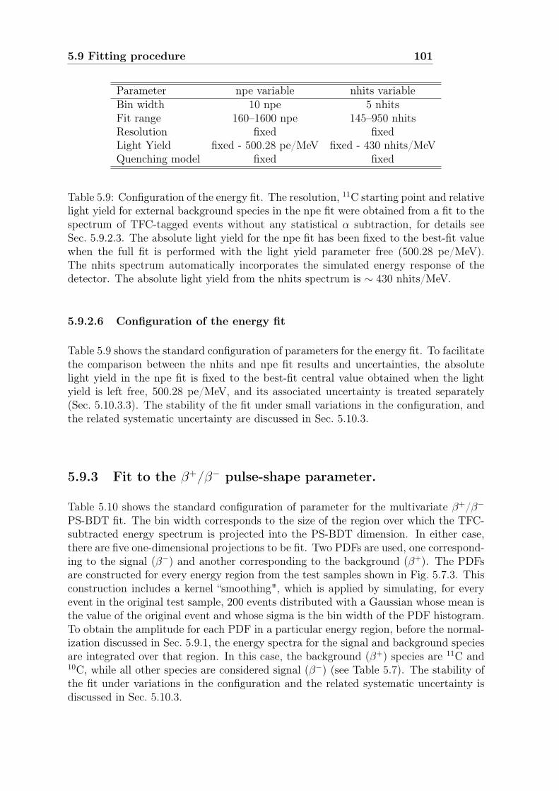
5.9 Fitting procedure 101
Parameter npe variable nhits variableBin width 10 npe 5 nhitsFit range 160–1600 npe 145–950 nhitsResolution fixed fixedLight Yield fixed - 500.28 pe/MeV fixed - 430 nhits/MeVQuenching model fixed fixed
Table 5.9: Configuration of the energy fit. The resolution, 11C starting point and relativelight yield for external background species in the npe fit were obtained from a fit to thespectrum of TFC-tagged events without any statistical α subtraction, for details seeSec. 5.9.2.3. The absolute light yield for the npe fit has been fixed to the best-fit valuewhen the full fit is performed with the light yield parameter free (500.28 pe/MeV).The nhits spectrum automatically incorporates the simulated energy response of thedetector. The absolute light yield from the nhits spectrum is ∼ 430 nhits/MeV.
5.9.2.6 Configuration of the energy fit
Table 5.9 shows the standard configuration of parameters for the energy fit. To facilitatethe comparison between the nhits and npe fit results and uncertainties, the absolutelight yield in the npe fit is fixed to the best-fit central value obtained when the lightyield is left free, 500.28 pe/MeV, and its associated uncertainty is treated separately(Sec. 5.10.3.3). The stability of the fit under small variations in the configuration, andthe related systematic uncertainty are discussed in Sec. 5.10.3.
5.9.3 Fit to the β+/β− pulse-shape parameter.
Table 5.10 shows the standard configuration of parameter for the multivariate β+/β−PS-BDT fit. The bin width corresponds to the size of the region over which the TFC-subtracted energy spectrum is projected into the PS-BDT dimension. In either case,there are five one-dimensional projections to be fit. Two PDFs are used, one correspond-ing to the signal (β−) and another corresponding to the background (β+). The PDFsare constructed for every energy region from the test samples shown in Fig. 5.7.3. Thisconstruction includes a kernel “smoothing", which is applied by simulating, for everyevent in the original test sample, 200 events distributed with a Gaussian whose mean isthe value of the original event and whose sigma is the bin width of the PDF histogram.To obtain the amplitude for each PDF in a particular energy region, before the normal-ization discussed in Sec. 5.9.1, the energy spectra for the signal and background speciesare integrated over that region. In this case, the background (β+) species are 11C and10C, while all other species are considered signal (β−) (see Table 5.7). The stability ofthe fit under variations in the configuration and the related systematic uncertainty isdiscussed in Sec. 5.10.3.
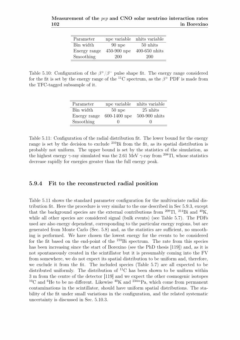
102Measurement of the pep and CNO solar neutrino interaction rates
in Borexino
Parameter npe variable nhits variableBin width 90 npe 50 nhitsEnergy range 450-900 npe 400-650 nhitsSmoothing 200 200
Table 5.10: Configuration of the β+/β− pulse shape fit. The energy range consideredfor the fit is set by the energy range of the 11C spectrum, as the β+ PDF is made fromthe TFC-tagged subsample of it.
Parameter npe variable nhits variableBin width 50 npe 25 nhitsEnergy range 600-1400 npe 500-900 nhitsSmoothing 0 0
Table 5.11: Configuration of the radial distribution fit. The lower bound for the energyrange is set by the decision to exclude 210Bi from the fit, as its spatial distribution isprobably not uniform. The upper bound is set by the statistics of the simulation, asthe highest energy γ-ray simulated was the 2.61 MeV γ-ray from 208Tl, whose statisticsdecrease rapidly for energies greater than the full energy peak.
5.9.4 Fit to the reconstructed radial position
Table 5.11 shows the standard parameter configuration for the multivariate radial dis-tribution fit. Here the procedure is very similar to the one described in Sec 5.9.3, exceptthat the background species are the external contributions from 208Tl, 214Bi and 40K,while all other species are considered signal (bulk events) (see Table 5.7). The PDFsused are also energy dependent, corresponding to the particular energy regions, but aregenerated from Monte Carlo (Sec. 5.8) and, as the statistics are sufficient, no smooth-ing is performed. We have chosen the lowest energy for the events to be consideredfor the fit based on the end-point of the 210Bi spectrum. The rate from this specieshas been increasing since the start of Borexino (see the PhD thesis [119]) and, as it isnot spontaneously created in the scintillator but it is presumably coming into the FVfrom somewhere, we do not expect its spatial distribution to be uniform and, therefore,we exclude it from the fit. The included species (Table 5.7) are all expected to bedistributed uniformly. The distribution of 11C has been shown to be uniform within3 m from the centre of the detector [119] and we expect the other cosmogenic isotopes10C and 6He to be no different. Likewise 40K and 234mPa, which come from permanentcontaminations in the scintillator, should have uniform spatial distributions. The sta-bility of the fit under small variations in the configuration, and the related systematicuncertainty is discussed in Sec. 5.10.3.

5.10 Results 103
5.10 Results
5.10.1 Fit result
The final fit result for the energy spectra are shown in Fig. 5.15 and 5.16, while thecorresponding best fits for the pulse-shape and radial distributions are shown in Fig. 5.17and 5.18, respectively. Fig. 5.19 shows the ∆χ2 profiles as a function of both pep ν andCNO νs interaction rates. The returned minimised − lnL values by the fit are in goodagreement with expectations (Sec. 5.10.2). Table 5.12 summarises the mean values,limits and statistical and systematic uncertainties (Sec. 5.10.3). As may be observedfrom the table, in both fits the CNO νs interaction rate is railed to zero. Therefore, wehave performed a likelihood ratio test (validated in Sec. 5.10.2) to estimate the upperlimits. Finally, Fig. 5.20 (left) shows the ∆χ2 profile from which these values have beenobtained. Fig. 5.21 presents the best fit value for the pep ν interaction rate when theCNO νs interaction rate is fixed at different values and Fig 5.20 (right) shows the ∆χ2
profile for the pep ν interaction rates.As may be observed in Fig. 5.15 and 5.16, the 11C, 10C and 6He rates are much
smaller in the spectrum of events after the TFC veto, as expected (Sec. 5.5.3). Withthe results from the fit we can estimate the fraction of 11C background after the vetoto be 0.094± 0.009.
The last column of Table 5.12 shows the expected rates for the fit species basedon other sources. For the pep ν and CNO νs interaction rates, the results are consis-tent with the expectations from both the High-Z and Low-Z SSMs. The results forthe cosmogenic isotopes 10C and 6He are also consistent with those obtained from ex-trapolations from KamLAND data (Sec. 5.3.2) and the value for 85Kr is ∼ 2σ awayfrom the one measured by the delayed coincidence method. The upper limits on the234mPa rate are lower than the expected value calculated from the 238U contaminationin the detector (Sec. 5.3.1). We note, though, that in the measurement of the 238Ucontamination, certain assumptions have been made regarding which and what fractionof the 214BiPo candidates are in secular equilibrium with 238U. Yet, as 214BiPo is muchfurther down the decay chain than 234mPa and can enter the fiducial volume, not onlyfrom 222Rn emanated by the vessels or from outside sources, but also from an originalcontamination of 226Ra in the scintillator, this value could be overestimated.
The measurement of the external background rates are at least a factor of 5 lower thanthe expectations. The γ-ray propagation from the PMTs to the FV by the Monte Carlohas been validated with the external radioactive source (Sec. 5.8) and, therefore, wesuspect that this disagreement is associated with the measurement of the radioactivityof the PMT components in [137]. Additionally, there is a ∼ 1σ difference between thevalues obtained for the 7Be ν interaction and 11C decay rates between this analysis andthe 7Be ν analysis [25]. This may be larger than expected, as the data sets used inthe two analyses have most events in common and, therefore, are strongly correlated.For the 7Be ν interaction rate, the discrepancy may be systematic, as the procedure toselect the central value (i.e. decide which fit configuration to consider “standard") wasdifferent. The systematic checks in Sec. 5.10.4.1 and 5.10.4.2 clarify this issue. As for11C, its production is cosmogenic and, therefore, its rate is not only time dependent butalso driven by high multiplicity events, making it much more sensitive to differences

104Measurement of the pep and CNO solar neutrino interaction rates
in Borexino
Component Central Value Statistical Unc. Systematic Unc. Expected valuecpd/100 tons cpd/100tons cpd/100tons cpd/100tons
pep ν 3.13 0.55 0.30 2.80± 0.047Be ν 48.3 2.0 0.9 46.0± 1.5± 1.685Kr 19.3 2.0 1.9 30.4± 5.3± 1.3210Bi 54.5 2.4 1.4 NA11C 27.4 0.3 0.1 28.5± 0.2± 0.710C 0.62 0.2 0.1 0.54± 0.046He 0.7 (0) 0.6 (0.5) 1 0.31± 0.04Ext. 208Tl 1.64 (1.94) 0.11 (0.13) 0.01 (0.02) > 5.7Ext. 214Bi 0.67 (0.41) 0.12 (0.13) 0.01 (0.02) > 6.6Ext. 40K 0.16 0.12 0.03 > 0.2Tot. Ext. γ 2.49 0.2 0.03 > 12.5
68% Limit 95% Limit 99% LimitCNO νs 4 12 19 5.4± 0.8 (3.8+0.6
−0.5)40K 0.11 0.42 0.69 NA234mPa 0.12 0.46 0.75 1.78± 0.06
Table 5.12: Table summarising the final results and their corresponding uncertainties.The statistical uncertainty is the one returned by the fitter, which has been validatedfor the pep ν interaction rate in Sec. 5.10.2. For 210Bi, the symmetric uncertaintyreturned by the fitter does not represent well the ∆χ2 profile, as can be suspected fromthe strong correlation with the CNO νs interaction rate (Fig. 5.22). For species thatare fit to zero, the upper confidence limits are obtained from the ∆χ2 profile, as inFig. 5.20 for CNO νs. The total systematic uncertainty has been obtained following themethodology outlined in Sec. 5.10.3. Differences between best-fit rates from the npeand nhits fits have been included within the systematic uncertainty, except for external208Tl and 214Bi, for which the rates and uncertainties are given separately i.e. npe(nhits). For the case of 6He, its central value is zero in the nhits fit and the numbergiven in parentheses for the uncertainty is the 68% U.L., while the corresponding 95%U.L. is 1.5 cpd/100tons. The last column shows the expected values for the differentspecies based on other sources. The expected interaction rates for pep ν and CNO νsare obtained from the latest High-Z (Low-Z) SSMs [60]. The expected rates for 7Be νinteractions and 11C decays are from the 7Be ν analysis [25]. The expected 85Kr ratecomes from the delayed coincidence analysis [25]. The expected rates for 234mPa and 10Cand 6He have already been presented in Tables 5.3 and 5.4, respectively. The expectedrates from backgrounds from the PMTs (Table 5.5) are taken as lower limits on thetotal external background. No previous valid estimates for 210Bi and 40K are available.

5.10 Results 105
Upper Limit CNO νs interaction rate Solar CNO νs flux % of total solar(pep ν rate @ SSM) cpd/100tons 108cm−2s−1 ν flux
68% 4.0± 1.3 3.9± 1.2 0.6± 0.295% 7.6± 1.2 7.4± 1.2 1.1± 0.299% 10.0± 1.1 9.7± 1.1 1.5± 0.2
Table 5.13: Upper limits for the CNO νs interaction rate when the pep ν interactionrate is fixed at the SSM prediction of 2.8 cpd/100tons. The corresponding ∆χ2 profilecan be seen in Fig. 5.20 (right). The uncertainties are systematic and were obtainedfollowing the methodology outlined in Sec. 5.10.3. The uncertainty introduced by thedifferences in the predicted pep ν flux from the High-Z and Low-Z SSMs is negligible.
Distributions considered pep ν 7Be ν 11C Ext. 214BiSingle energy spectrum 0.6± 2.8 50.2± 3.0 1.66± 0.60 0.64± 0.24Only energy spectra 2.44± 0.80 49.9± 1.9 1.82± 0.48 0.40± 0.23Energy spectra + radial dist 3.75± 0.96 50.0± 1.9 1.41± 0.41 0.73± 0.13Energy spectra + PS-BDT 3.37± 0.55 48.4± 1.8 2.78± 0.17 0.44± 0.16No complementary spectrum 3.45± 0.64 47.9± 1.8 2.46± 0.16 0.72± 0.13All 3.33± 0.57 48.3± 1.7 2.48± 0.16 0.68± 0.12
Table 5.14: Differences in the central values and uncertainties of some characteristicspecies returned by the fit with the standard options (Tables 5.7, 5.9, 5.10 and 5.11)when different event distributions are included; the energy estimator is npe; central valueand uncertainties are expressed in cpd/100tons. The 11C rate presented corresponds tothe one in the TFC-subtracted spectrum. The results from the last row are those fromthe full fit result presented in Fig. 5.16, 5.17 (right) and 5.18 (right). The uncertaintyin the rates decrease as more distributions are considered. The distribution whoseinclusion in the fit has the greatest effect in the pep ν interaction rate uncertainty isthat of the PS-BDT parameter. Differences in the central values are also observed and,for the case of the ν interaction rates, these are smaller than the fit uncertainty.
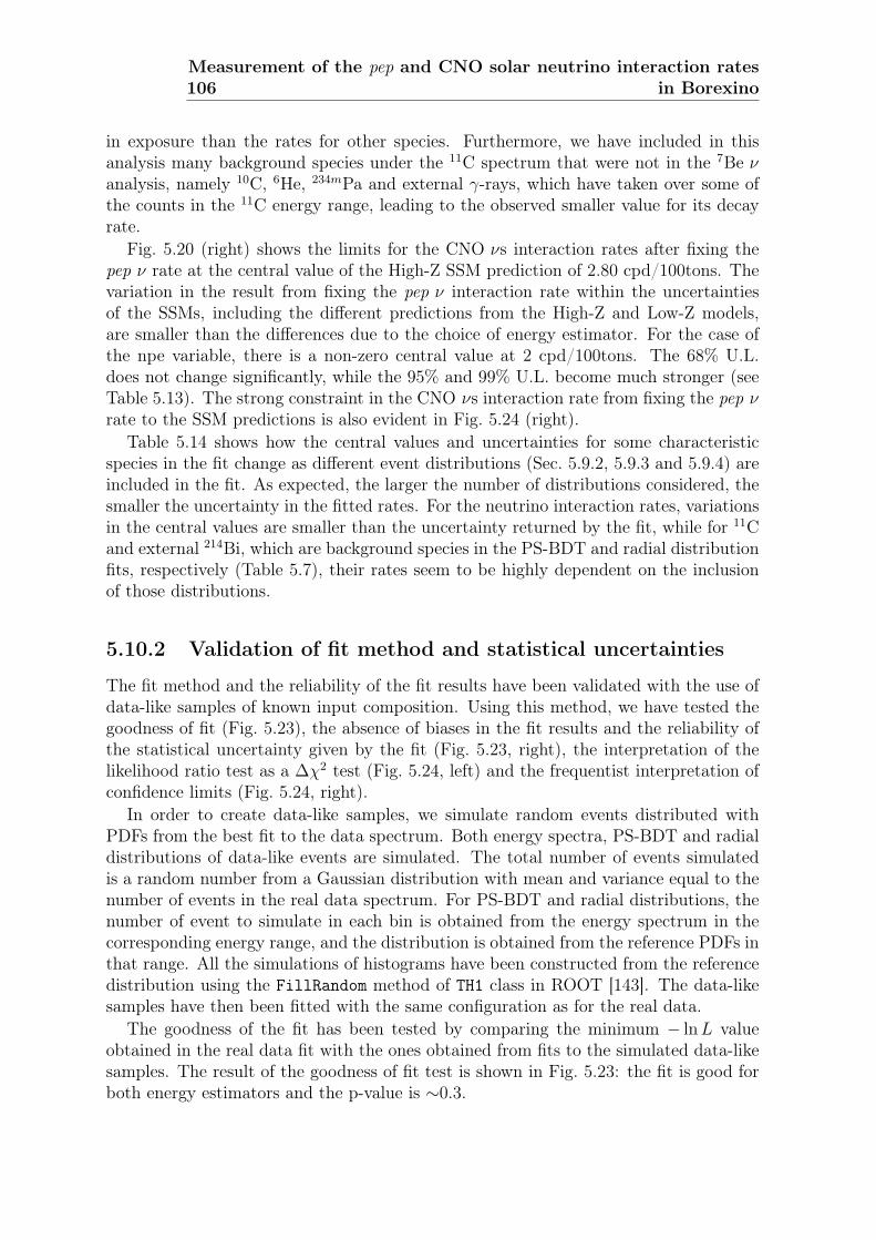
106Measurement of the pep and CNO solar neutrino interaction rates
in Borexino
in exposure than the rates for other species. Furthermore, we have included in thisanalysis many background species under the 11C spectrum that were not in the 7Be νanalysis, namely 10C, 6He, 234mPa and external γ-rays, which have taken over some ofthe counts in the 11C energy range, leading to the observed smaller value for its decayrate.
Fig. 5.20 (right) shows the limits for the CNO νs interaction rates after fixing thepep ν rate at the central value of the High-Z SSM prediction of 2.80 cpd/100tons. Thevariation in the result from fixing the pep ν interaction rate within the uncertaintiesof the SSMs, including the different predictions from the High-Z and Low-Z models,are smaller than the differences due to the choice of energy estimator. For the case ofthe npe variable, there is a non-zero central value at 2 cpd/100tons. The 68% U.L.does not change significantly, while the 95% and 99% U.L. become much stronger (seeTable 5.13). The strong constraint in the CNO νs interaction rate from fixing the pep νrate to the SSM predictions is also evident in Fig. 5.24 (right).
Table 5.14 shows how the central values and uncertainties for some characteristicspecies in the fit change as different event distributions (Sec. 5.9.2, 5.9.3 and 5.9.4) areincluded in the fit. As expected, the larger the number of distributions considered, thesmaller the uncertainty in the fitted rates. For the neutrino interaction rates, variationsin the central values are smaller than the uncertainty returned by the fit, while for 11Cand external 214Bi, which are background species in the PS-BDT and radial distributionfits, respectively (Table 5.7), their rates seem to be highly dependent on the inclusionof those distributions.
5.10.2 Validation of fit method and statistical uncertainties
The fit method and the reliability of the fit results have been validated with the use ofdata-like samples of known input composition. Using this method, we have tested thegoodness of fit (Fig. 5.23), the absence of biases in the fit results and the reliability ofthe statistical uncertainty given by the fit (Fig. 5.23, right), the interpretation of thelikelihood ratio test as a ∆χ2 test (Fig. 5.24, left) and the frequentist interpretation ofconfidence limits (Fig. 5.24, right).
In order to create data-like samples, we simulate random events distributed withPDFs from the best fit to the data spectrum. Both energy spectra, PS-BDT and radialdistributions of data-like events are simulated. The total number of events simulatedis a random number from a Gaussian distribution with mean and variance equal to thenumber of events in the real data spectrum. For PS-BDT and radial distributions, thenumber of event to simulate in each bin is obtained from the energy spectrum in thecorresponding energy range, and the distribution is obtained from the reference PDFs inthat range. All the simulations of histograms have been constructed from the referencedistribution using the FillRandom method of TH1 class in ROOT [143]. The data-likesamples have then been fitted with the same configuration as for the real data.
The goodness of the fit has been tested by comparing the minimum − lnL valueobtained in the real data fit with the ones obtained from fits to the simulated data-likesamples. The result of the goodness of fit test is shown in Fig. 5.23: the fit is good forboth energy estimators and the p-value is ∼0.3.
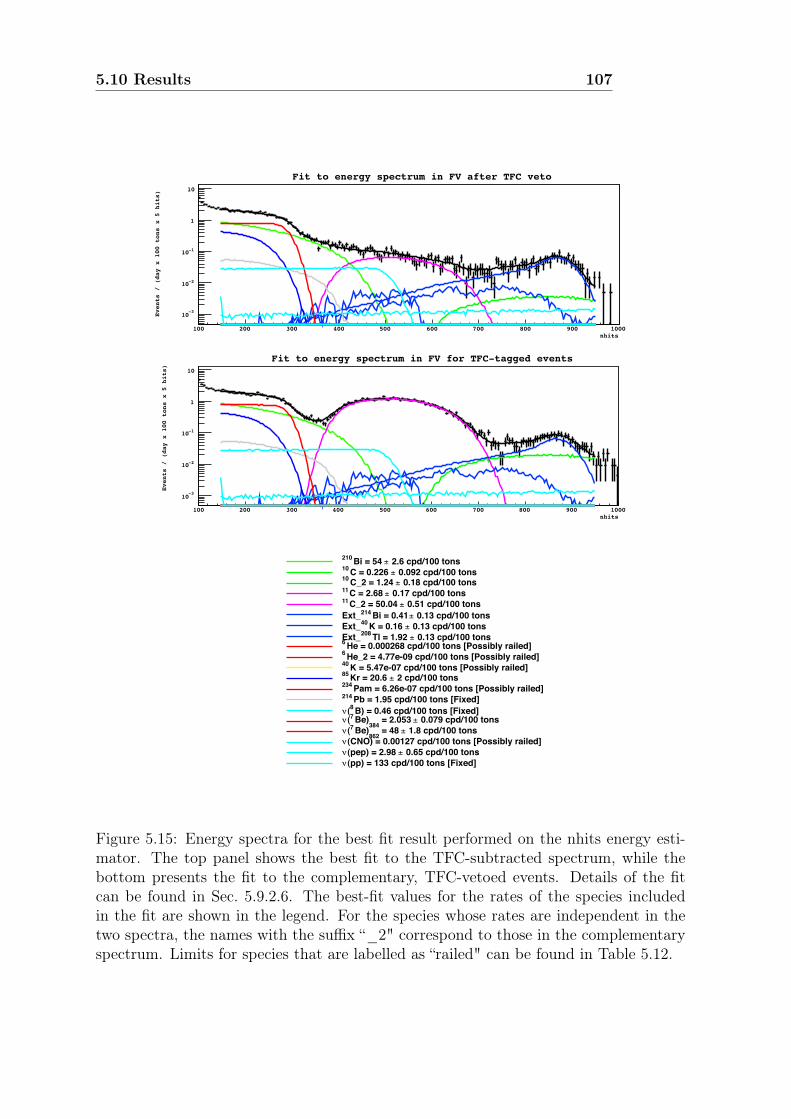
5.10 Results 107
Photoelectrons [Light yield = 502 p.e./MeV [Fixed]]0 200 400 600 800 1000 1200 1400 1600 1800 2000
Events / (day x 100 tons x 5 p.e.)
2
4
6
8
10
12
Data from 20409.1 days x tons livetime / N-DOF = 371.294 / 3052!Total spectrum,
2.6 cpd/100 tons±Bi = 54 210
0.092 cpd/100 tons±C = 0.226 10
0.18 cpd/100 tons±C_2 = 1.24 10
0.17 cpd/100 tons±C = 2.68 11
0.51 cpd/100 tons±C_2 = 50.04 11
0.13 cpd/100 tons±Bi = 0.41 214 Ext_ 0.13 cpd/100 tons±K = 0.16 40 Ext_ 0.13 cpd/100 tons±Tl = 1.92 208 Ext_
He = 0.000268 cpd/100 tons [Possibly railed]6
He_2 = 4.77e-09 cpd/100 tons [Possibly railed]6
K = 5.47e-07 cpd/100 tons [Possibly railed]40
2 cpd/100 tons±Kr = 20.6 85
Pam = 6.26e-07 cpd/100 tons [Possibly railed]234
Pb = 1.95 cpd/100 tons [Fixed]214
B) = 0.46 cpd/100 tons [Fixed]8 (" 0.079 cpd/100 tons± = 2.053
384Be)7 ("
1.8 cpd/100 tons± = 48 862
Be)7 ("(CNO) = 0.00127 cpd/100 tons [Possibly railed]"
0.65 cpd/100 tons±(pep) = 2.98 "(pp) = 133 cpd/100 tons [Fixed]"
Spectrum after Step 3#
0 200 400 600 800 1000 1200 1400 1600 1800 2000
0
1
2
3
4
5
6
7
8
9
Spectrum after Step 3#
nhits100 200 300 400 500 600 700 800 900 1000
Events / (day x 100 tons x 5 hits)
-310
-210
-110
1
10
Fit to energy spectrum in FV after TFC veto
nhits100 200 300 400 500 600 700 800 900 1000
Events / (day x 100 tons x 5 hits)
-310
-210
-110
1
10
Fit to energy spectrum in FV for TFC-tagged events
Figure 5.15: Energy spectra for the best fit result performed on the nhits energy esti-mator. The top panel shows the best fit to the TFC-subtracted spectrum, while thebottom presents the fit to the complementary, TFC-vetoed events. Details of the fitcan be found in Sec. 5.9.2.6. The best-fit values for the rates of the species includedin the fit are shown in the legend. For the species whose rates are independent in thetwo spectra, the names with the suffix “_2" correspond to those in the complementaryspectrum. Limits for species that are labelled as “railed" can be found in Table 5.12.

108Measurement of the pep and CNO solar neutrino interaction rates
in Borexino
npe200 400 600 800 1000 1200 1400 1600
Events / (day x 100 tons x 10 p.e.)
-310
-210
-110
1
10
Fit to energy spectrum in FV after TFC veto
npe200 400 600 800 1000 1200 1400 1600
Events / (day x 100 tons x 10 p.e.)
-310
-210
-110
1
10
Fit to energy spectrum in FV for TFC-tagged events
Photoelectrons [Light yield = 502 p.e./MeV [Fixed]]0 200 400 600 800 1000 1200 1400 1600 1800 2000
Events / (day x 100 tons x 10 p.e.)
2
4
6
8
10
12
Data from 20409.1 days x tons livetime / N-DOF = 358.321 / 2622!Total spectrum,
2.4 cpd/100 tons±Bi = 53.9 210
0.071 cpd/100 tons±C = 0.181 10
0.45 cpd/100 tons±C_2 = 0.91 10
0.16 cpd/100 tons±C = 2.48 11
0.65 cpd/100 tons±C_2 = 50.02 11
0.12 cpd/100 tons±Bi = 0.68 214 Ext_ 0.11 cpd/100 tons±K = 0.21 40 Ext_
0.11 cpd/100 tons±Tl = 1.63 208 Ext_He = 6.6e-08 cpd/100 tons [Possibly railed]6
1.1 cpd/100 tons±He_2 = 1.3 6
K = 2.64e-08 cpd/100 tons [Possibly railed]40
2 cpd/100 tons±Kr = 19.9 85
Pam = 3.89e-08 cpd/100 tons [Possibly railed]234
Pb = 1.95 cpd/100 tons [Fixed]214
B) = 0.46 cpd/100 tons [Fixed]8 (" 0.071 cpd/100 tons± = 2.067
384Be)7 ("
1.7 cpd/100 tons± = 48.3 862
Be)7 ("(CNO) = 1.15e-07 cpd/100 tons [Possibly railed]"
0.57 cpd/100 tons±(pep) = 3.33 "(pp) = 133 cpd/100 tons [Fixed]"
Spectrum after Step 3#
0 200 400 600 800 1000 1200 1400 1600 1800 20000
10000
20000
30000
40000
50000
Spectrum after Step 3#
Figure 5.16: Energy spectra for the best fit result performed on the npe energy esti-mator. The top panel shows the best fit to the TFC-subtracted spectrum, while thebottom presents the fit to the complementary, TFC-vetoed events. Details of the fitcan be found in Sec. 5.9.2.6. The best-fit values for the rates of the species includedin the fit are shown in the legend. For the species whose rates are independent in thetwo spectra, the names with the suffix “_2" correspond to those in the complementaryspectrum. Limits for species that are labelled as “railed" can be found in Table 5.12.

5.10 Results 109
PS-BDT Parameter-0.6 -0.4 -0.2 0 0.2 0.40
20
40
60
80
100
120
Distribution of pulse-shape parameter
Data
Signal
Background
/NDF = 44.6/462χBest Fit -
PS-BDT Parameter-1 -0.8 -0.6 -0.4 -0.2 0 0.2 0.4 0.6 0.8 1
1
10
210
Data
Signal
Background
/NDF = 46.6/482χBest Fit -
Distribution of pulse-shape parameter
Figure 5.17: Left panel: Distribution of PS-BDT parameter in the energy range 400–650 nhits. Right panel: Distribution of PS-BDT parameter in the energy range 450–900 npe; the scale is logarithmic. In both cases, the total PDF distribution from thebest-fit result is shown, as well as the result from a χ2-test to evaluate the goodness ofthe fit.
Reconstructed event radius / m0 0.5 1 1.5 2 2.5 3
1
10
210
DataSignal
Background
/NDF = 23.3/272χBest Fit -
Radial distribution of candidates
Reconstructed event radius / m0 0.5 1 1.5 2 2.5 30
20406080100120140160180200220240
DataSignalBackground
/NDF = 29.4/272χBest Fit -
Radial distribution of candidates
Figure 5.18: Left panel: Radial distribution of events in the energy range 500–900nhits; the scale is logarithmic. Right panel: Radial distribution of events in theenergy range 600–1400 npe. In both cases, the total PDF distribution from the best-fitresult is shown, as well as the result from a χ2-test to evaluate the goodness of the fit.
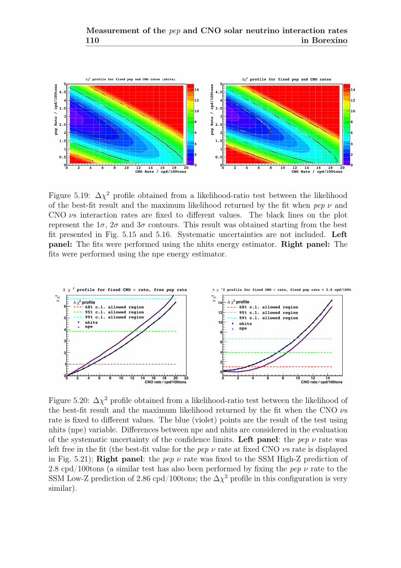
110Measurement of the pep and CNO solar neutrino interaction rates
in Borexino
CNO Rate / cpd/100tons0 2 4 6 8 10 12 14 16 18 20
pep
Rate
/ c
pd/1
00to
ns
0
0.5
1
1.5
2
2.5
3
3.5
4
4.5
5
0
2
4
6
8
10
12
14
profile for fixed pep and CNO rates (nhits)2!"
0 2 4 6 8 10 12 14 16 18 200
0.5
1
1.5
2
2.5
3
3.5
4
4.5
5h2c
CNO Rate / cpd/100tons0 2 4 6 8 10 12 14 16 18 20
pep
Rate
/ c
pd/1
00to
ns
0
0.5
1
1.5
2
2.5
3
3.5
4
4.5
5
0
2
4
6
8
10
12
14
profile for fixed pep and CNO rates2!"
0 2 4 6 8 10 12 14 16 18 200
0.5
1
1.5
2
2.5
3
3.5
4
4.5
5
cno_pep_c
Figure 5.19: ∆χ2 profile obtained from a likelihood-ratio test between the likelihoodof the best-fit result and the maximum likelihood returned by the fit when pep ν andCNO νs interaction rates are fixed to different values. The black lines on the plotrepresent the 1σ, 2σ and 3σ contours. This result was obtained starting from the bestfit presented in Fig. 5.15 and 5.16. Systematic uncertainties are not included. Leftpanel: The fits were performed using the nhits energy estimator. Right panel: Thefits were performed using the npe energy estimator.
CNO rate / cpd/100tons0 2 4 6 8 10 12 14 16 18 20 22
2 χ Δ
0
1
2
3
4
5
6 profile2χ Δ68% c.l. allowed region95% c.l. allowed region99% c.l. allowed regionnhitsnpe
rate, free pep rateν profile for fixed CNO 2 χ Δ
CNO rate / cpd/100tons0 2 4 6 8 10 12 14
2 χ Δ
0
2
4
6
8
10
12
14 profile2χ Δ68% c.l. allowed region95% c.l. allowed region99% c.l. allowed regionnhitsnpe
rate, fixed pep rate = 2.8 cpd/100tν ^2 profile for fixed CNO χ Δ
Figure 5.20: ∆χ2 profile obtained from a likelihood-ratio test between the likelihood ofthe best-fit result and the maximum likelihood returned by the fit when the CNO νsrate is fixed to different values. The blue (violet) points are the result of the test usingnhits (npe) variable. Differences between npe and nhits are considered in the evaluationof the systematic uncertainty of the confidence limits. Left panel: the pep ν rate wasleft free in the fit (the best-fit value for the pep ν rate at fixed CNO νs rate is displayedin Fig. 5.21); Right panel: the pep ν rate was fixed to the SSM High-Z prediction of2.8 cpd/100tons (a similar test has also been performed by fixing the pep ν rate to theSSM Low-Z prediction of 2.86 cpd/100tons; the ∆χ2 profile in this configuration is verysimilar).
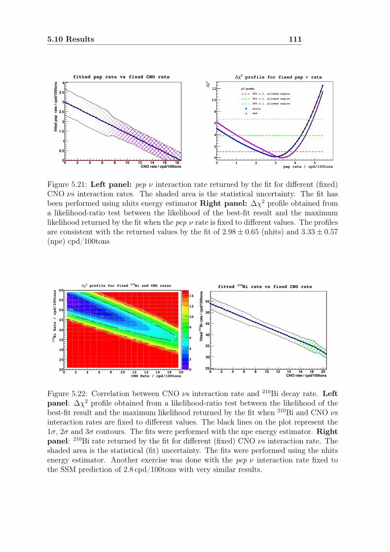
5.10 Results 111
CNO rate / cpd/100tons0 2 4 6 8 10 12 14 16 18
fitte
d pe
p ra
te /
cpd/
100t
ons
0
0.5
1
1.5
2
2.5
3
3.5
4fitted pep rate vs fixed CNO rate
pep rate / cpd/100tons0 1 2 3 4 5
2 χ∆
0
2
4
6
8
10
12 profile2χ∆
68% c.l. allowed region
95% c.l. allowed region
99% c.l. allowed region
nhits
npe
rateν profile for fixed pep 2χ∆
Figure 5.21: Left panel: pep ν interaction rate returned by the fit for different (fixed)CNO νs interaction rates. The shaded area is the statistical uncertainty. The fit hasbeen performed using nhits energy estimator Right panel: ∆χ2 profile obtained froma likelihood-ratio test between the likelihood of the best-fit result and the maximumlikelihood returned by the fit when the pep ν rate is fixed to different values. The profilesare consistent with the returned values by the fit of 2.98± 0.65 (nhits) and 3.33± 0.57(npe) cpd/100tons
CNO Rate / cpd/100tons0 2 4 6 8 10 12 14 16 18 20
Bi R
ate
/ cp
d/10
0ton
s210
20
25
30
35
40
45
50
55
60
0
2
4
6
8
10
12
14
Bi and CNO rates210 profile for fixed 2!"
0 2 4 6 8 10 12 14 16 18 2020
25
30
35
40
45
50
55
60h2c
CNO rate / cpd/100tons0 2 4 6 8 10 12 14 16 18 20
Bi ra
te /
cpd/
100t
ons
210
fitte
d
25
30
35
40
45
50
55
Bi rate vs fixed CNO rate210fitted
Figure 5.22: Correlation between CNO νs interaction rate and 210Bi decay rate. Leftpanel: ∆χ2 profile obtained from a likelihood-ratio test between the likelihood of thebest-fit result and the maximum likelihood returned by the fit when 210Bi and CNO νsinteraction rates are fixed to different values. The black lines on the plot represent the1σ, 2σ and 3σ contours. The fits were performed with the npe energy estimator. Rightpanel: 210Bi rate returned by the fit for different (fixed) CNO νs interaction rate. Theshaded area is the statistical (fit) uncertainty. The fits were performed using the nhitsenergy estimator. Another exercise was done with the pep ν interaction rate fixed tothe SSM prediction of 2.8 cpd/100tons with very similar results.
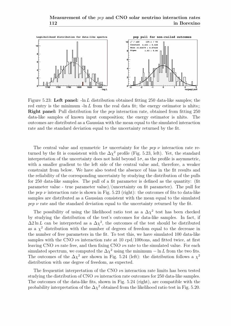
112Measurement of the pep and CNO solar neutrino interaction rates
in Borexino
- log L1740 1760 1780 1800 1820 18400
2
4
6
8
10
LogLikelihood distribution for data-like spectra
/ ndf 2χ 129.1 / 92Constant 0.420± 4.631 Mean 0.07620± -0.03679 Sigma 0.06± 1.03
nu(pep) pull-3 -2 -1 0 1 2 30
2
4
6
8
10 / ndf 2χ 129.1 / 92Constant 0.420± 4.631 Mean 0.07620± -0.03679 Sigma 0.06± 1.03
pep pull for non-railed outcomes
Figure 5.23: Left panel: -lnL distribution obtained fitting 250 data-like samples; thered entry is the minimum -lnL from the real data fit; the energy estimator is nhits;;Right panel: Pull distribution for the pep interaction rate, obtained from fitting 250data-like samples of known input composition; the energy estimator is nhits. Theoutcomes are distributed as a Gaussian with the mean equal to the simulated interactionrate and the standard deviation equal to the uncertainty returned by the fit.
The central value and symmetric 1σ uncertainty for the pep ν interaction rate re-turned by the fit is consistent with the ∆χ2 profile (Fig. 5.23, left). Yet, the standardinterpretation of the uncertainty does not hold beyond 1σ, as the profile is asymmetric,with a smaller gradient to the left side of the central value and, therefore, a weakerconstraint from below. We have also tested the absence of bias in the fit results andthe reliability of the corresponding uncertainty by studying the distribution of the pullsfor 250 data-like samples. The pull of a fit parameter is defined as the quantity: (fitparameter value - true parameter value)/(uncertainty on fit parameter). The pull forthe pep ν interaction rate is shown in Fig. 5.23 (right): the outcomes of fits to data-likesamples are distributed as a Gaussian consistent with the mean equal to the simulatedpep ν rate and the standard deviation equal to the uncertainty returned by the fit.
The possibility of using the likelihood ratio test as a ∆χ2 test has been checkedby studying the distribution of the test’s outcomes for data-like samples. In fact, if∆2 lnL can be interpreted as a ∆χ2, the outcomes of the test should be distributedas a χ2 distribution with the number of degrees of freedom equal to the decrease inthe number of free parameters in the fit. To test this, we have simulated 100 data-likesamples with the CNO νs interaction rate at 10 cpd/100tons, and fitted twice, at firstleaving CNO νs rate free, and then fixing CNO νs rate to the simulated value. For eachsimulated spectrum, we computed the ∆χ2 using the minimum − lnL from the two fits.The outcomes of the ∆χ2 are shown in Fig. 5.24 (left): the distribution follows a χ2
distribution with one degree of freedom, as expected.
The frequentist interpretation of the CNO νs interaction rate limits has been testedstudying the distribution of CNO νs interaction rate outcomes for 250 data-like samples.The outcomes of the data-like fits, shown in Fig. 5.24 (right), are compatible with theprobability interpretation of the ∆χ2 obtained from the likelihood ratio test in Fig. 5.20.
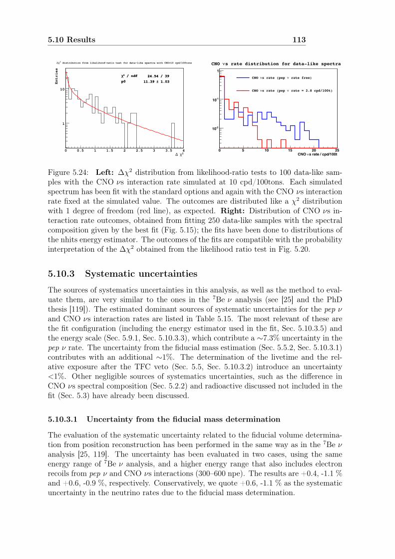
5.10 Results 113
/ ndf 2χ 24.54 / 39
p0 1.03± 11.39
2χ ∆0 0.5 1 1.5 2 2.5 3 3.5 4
Entries
1
10
/ ndf 2χ 24.54 / 39
p0 1.03± 11.39
distribution from likelihood-ratio test for data-like spectra with CNO=10 cpd/100tons2χ∆
s rate / cpd/100tν CNO 0 5 10 15 20 25
-210
-110
1
s rate distribution for data-like spectraνCNO
rate free)νs rate (pep νCNO
rate = 2.8 cpd/100t) νs rate (pep νCNO
Figure 5.24: Left: ∆χ2 distribution from likelihood-ratio tests to 100 data-like sam-ples with the CNO νs interaction rate simulated at 10 cpd/100tons. Each simulatedspectrum has been fit with the standard options and again with the CNO νs interactionrate fixed at the simulated value. The outcomes are distributed like a χ2 distributionwith 1 degree of freedom (red line), as expected. Right: Distribution of CNO νs in-teraction rate outcomes, obtained from fitting 250 data-like samples with the spectralcomposition given by the best fit (Fig. 5.15); the fits have been done to distributions ofthe nhits energy estimator. The outcomes of the fits are compatible with the probabilityinterpretation of the ∆χ2 obtained from the likelihood ratio test in Fig. 5.20.
5.10.3 Systematic uncertainties
The sources of systematics uncertainties in this analysis, as well as the method to eval-uate them, are very similar to the ones in the 7Be ν analysis (see [25] and the PhDthesis [119]). The estimated dominant sources of systematic uncertainties for the pep νand CNO νs interaction rates are listed in Table 5.15. The most relevant of these arethe fit configuration (including the energy estimator used in the fit, Sec. 5.10.3.5) andthe energy scale (Sec. 5.9.1, Sec. 5.10.3.3), which contribute a ∼7.3% uncertainty in thepep ν rate. The uncertainty from the fiducial mass estimation (Sec. 5.5.2, Sec. 5.10.3.1)contributes with an additional ∼1%. The determination of the livetime and the rel-ative exposure after the TFC veto (Sec. 5.5, Sec. 5.10.3.2) introduce an uncertainty<1%. Other negligible sources of systematics uncertainties, such as the difference inCNO νs spectral composition (Sec. 5.2.2) and radioactive discussed not included in thefit (Sec. 5.3) have already been discussed.
5.10.3.1 Uncertainty from the fiducial mass determination
The evaluation of the systematic uncertainty related to the fiducial volume determina-tion from position reconstruction has been performed in the same way as in the 7Be νanalysis [25, 119]. The uncertainty has been evaluated in two cases, using the sameenergy range of 7Be ν analysis, and a higher energy range that also includes electronrecoils from pep ν and CNO νs interactions (300–600 npe). The results are +0.4, -1.1 %and +0.6, -0.9 %, respectively. Conservatively, we quote +0.6, -1.1 % as the systematicuncertainty in the neutrino rates due to the fiducial mass determination.
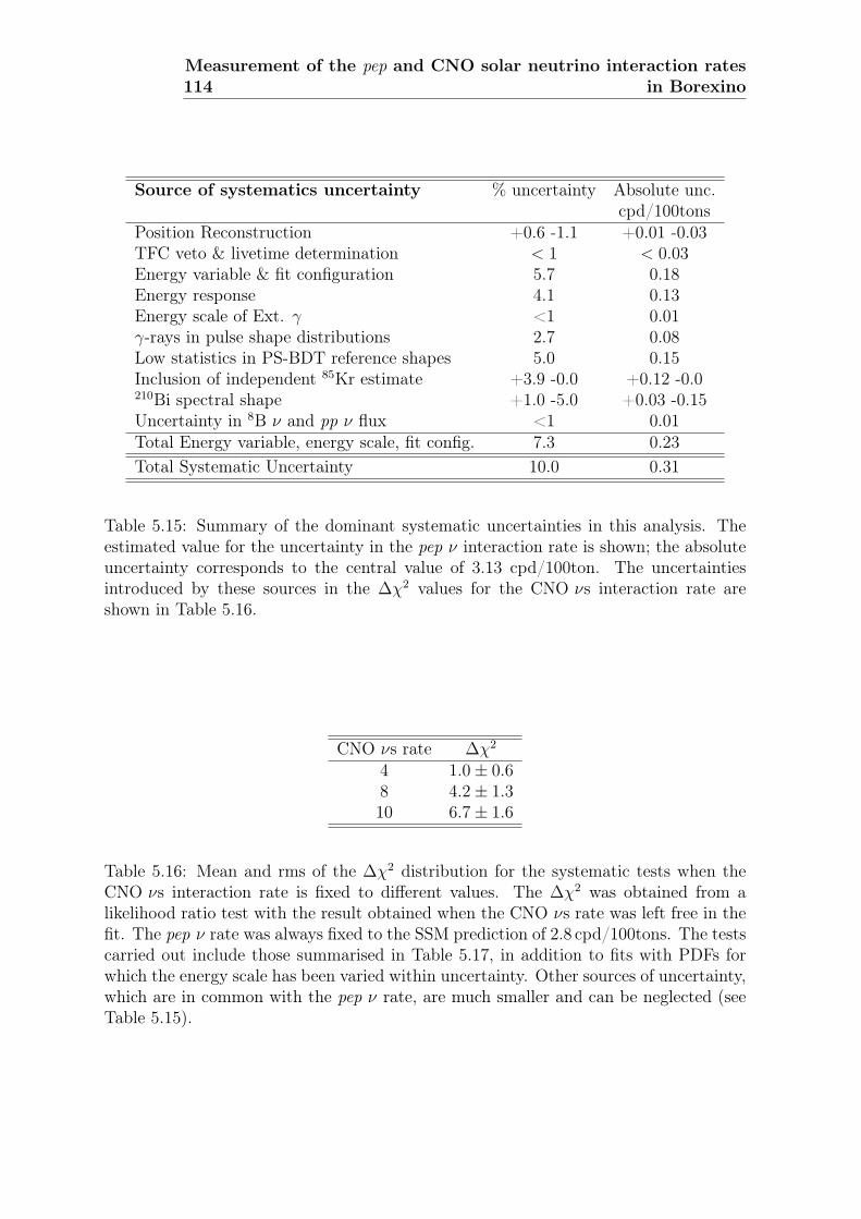
114Measurement of the pep and CNO solar neutrino interaction rates
in Borexino
Source of systematics uncertainty % uncertainty Absolute unc.cpd/100tons
Position Reconstruction +0.6 -1.1 +0.01 -0.03TFC veto & livetime determination < 1 < 0.03Energy variable & fit configuration 5.7 0.18Energy response 4.1 0.13Energy scale of Ext. γ <1 0.01γ-rays in pulse shape distributions 2.7 0.08Low statistics in PS-BDT reference shapes 5.0 0.15Inclusion of independent 85Kr estimate +3.9 -0.0 +0.12 -0.0210Bi spectral shape +1.0 -5.0 +0.03 -0.15Uncertainty in 8B ν and pp ν flux <1 0.01Total Energy variable, energy scale, fit config. 7.3 0.23Total Systematic Uncertainty 10.0 0.31
Table 5.15: Summary of the dominant systematic uncertainties in this analysis. Theestimated value for the uncertainty in the pep ν interaction rate is shown; the absoluteuncertainty corresponds to the central value of 3.13 cpd/100ton. The uncertaintiesintroduced by these sources in the ∆χ2 values for the CNO νs interaction rate areshown in Table 5.16.
CNO νs rate ∆χ2
4 1.0± 0.68 4.2± 1.310 6.7± 1.6
Table 5.16: Mean and rms of the ∆χ2 distribution for the systematic tests when theCNO νs interaction rate is fixed to different values. The ∆χ2 was obtained from alikelihood ratio test with the result obtained when the CNO νs rate was left free in thefit. The pep ν rate was always fixed to the SSM prediction of 2.8 cpd/100tons. The testscarried out include those summarised in Table 5.17, in addition to fits with PDFs forwhich the energy scale has been varied within uncertainty. Other sources of uncertainty,which are in common with the pep ν rate, are much smaller and can be neglected (seeTable 5.15).
5.10 Results 115
5.10.3.2 Uncertainty from the livetime and relative exposure
The computation of the livetime prior to the TFC veto has been performed in thesame way of the 7Be ν analysis [25]. The related systematic uncertainty is smallerthan the loss of exposure due to fast coincidences (see the PhD thesis [119]), whichhas not been corrected for in this analysis. As this correction is much smaller thanthe systematic uncertainty arising from to the fit configuration and energy scale (Table5.15), a more precise evaluation is not necessary. The statistical uncertainty associatedwith the counting method used to estimate the relative exposure after the TFC vetoes(Sec. 5.5.3) is < 0.5%, due to the large number of events considered (210Po or simulated).The discrepancy between the two methods, which is < 1%, is possibly due to systematiceffects associated with the non-uniform spatial and time distribution of the 210Po andcan be considered an upper limit on the accuracy of the method. Overall, we quote anuncertainty in the exposure introduced by the livetime estimation and the TFC vetothat is < 1%.
5.10.3.3 Uncertainty from the energy scale
The calibration of the energy scale has been discussed in Sec. 4.3.1 and Sec. 5.9. Tostudy the systematic uncertainty in the pep ν rate associated with it, we took differentapproaches for the different energy estimators.
For the nhits energy estimator, we performed fits using energy spectra PDFs withdifferent energy scale parameters that are ±2σ from the best-fit value, as determinedby likelihood-ratio tests. For the light yield, the scaling used to produce the spectrawas ±0.2% from the best fit value. We also considred a PDF with the light yield scaledby -0.4% and with the 11C spectrum shifted by 4 hits, as well as one with worseneddetector resolution. Considering the differences between the best-fit pep ν rate andthose obtained from fits with these PDFs, we estimate a 1σ uncertainty in the pep νinteraction rate of 4.1%.
To estimate the corresponding uncertainty in the fit to the npe energy estimator,we have done a scan on the light yield about the best fit central value of 500 pe/MeV,noting the change in minimised − lnL. We have kept the effective light yield of theexternal background species (in pe/MeV) and the starting point of the 11C spectrum(in npe) to their best-fit values. The 1σ uncertainty in the light yield for uniform speciesis determined to be ±2 pe/MeV and the associated uncertainty in the pep ν interactionrate is 1.7%. Additionally, to evaluate the effect of the energy resolution in the pep νinteraction rate, we performed a fit with the resolution parameters set to +2σ of theresult obtained from the fit to the 210Po energy peak. The interaction rate increased by0.3%, which is a negligible effect.
5.10.3.4 Energy scale of external background spectrum
In order to align the peak of the simulated 208Tl energy spectrum (Sec. 5.8, Fig. 5.14), tothe peak of the real data 208Tl, a shift of 5 nhits (over ∼900 nhits) is needed. In order toevaluate the effect of the uncertainties of the external background energy scale, we havecompared the results of the fit with the 208Tl spectrum shifted of 5 nhits, the fit with no

116Measurement of the pep and CNO solar neutrino interaction rates
in Borexino
Parameter npe variable nhits variableEnergy variable npe nhitsBin width 5, 10 5, 10Fit start point 160, 165, 170 140, 145, 150Fit end point 1560–1640 920–960PS-BDT Bin width 90, 100, 120 50, 110, 120PS-BDT start point 400, 450 400-430PS-BDT end point 880–900 620-680PS-BDT Smoothing 180–220 180–220Rdist Bin width 40, 50, 70 25, 40Rdist start point 580–620 490-510Rdist end point 1380–1440 890-910214Pb rate 1.95±0.07 1.95±0.07
Table 5.17: Variation in the parameter configuration of the fit for the systematics study.In the case of the 214Pb rate, we vary the fixed rate according to a Gaussian distributionwith the specified σ.
shift in 208Tl spectrum, and the fit with a corresponding scale (instead of a shift) in the208Tl spectrum. For every of this checks, the change in pep ν fitted rate is less than 1%:in the first case (standard fit, 5 nhits shift), the pep ν rate is 2.98±0.65 cpd/100tons,in the second case (no shift), the pep ν rate is 2.97±0.66 cpd/100tons, in the third case(scale instead of shift) the pep ν rate is 2.99±0.66 cpd/100tons. Also the 208Tl fittedrate is changed by less than 1% among the three checks.
5.10.3.5 Uncertainty from the fit configuration
The fit method and fit parameters configuration has been described in Sec. 5.9. To studythe stability of the fit under small variations in the configuration, and to evaluate thecorresponding systematics uncertainties in the neutrino interaction rates, we performeda large number of fits, randomly changing the configuration parameters. We havetaken the rms of the pep ν rate distribution as the systematic uncertainty from thefit configuration. For the case of the CNO νs rate, where we quote upper limits, wehave performed likelihood ratio tests under different fit configurations and from theresulting distribution of the ∆χ2 obtained values for its mean and uncertainty (rms ofthe distribution). From these we can then extract the systematic uncertainty in theconfidence limits. The range of allowed configuration parameters used to evaluate thesystematic uncertainty is listed in Table 5.17. The energy estimator (and correspondingspectrum) used for the fit is included as one of the configuration parameters to vary. Wequote 5.7% as the systematic uncertainty in the pep ν rate due to the fit configuration.
5.10 Results 117
5.10.3.6 Uncertainty from the presence of γ-ray events in PS-BDT fit
In order to exclude from the PS-BDT distributions the 214Bi events in the test samplethat have some considerable contribution from γ-rays (Sec. 5.7.3), as well as most ofthe external γ-ray background from the data, we have decreased the energy end pointof the PS-BDT fit to 700 npe. In this case, the resulting value for the pep ν rate inthe npe fit changes from 3.33± 0.57 to 3.42± 0.51 cpd/100tons, a 2.7% increase in thecentral value.
5.10.3.7 Uncertainty from the limited statistics in reference PS-BDT dis-tributions
The impact of the limited statistics in the reference PS-BDT distributions has beendetermined by performing fits where the bin content of of the reference shapes wasrandomly modified according to Poisson statistics. We have taken the rms of the pep νrate distribution as the systematic uncertainty from the fit configuration. The resultingpep ν interaction rate follows a Gaussian distribution with σ/µ = 0.05. We quote 5% asthe systematic uncertainty in the pep ν rate due to the limited statistics in the referencePS-BDT distributions.
5.10.3.8 Introduction of the independent 85Kr estimate in the fit
As discussed in Sec. 5.10.1, the 85Kr value returned by the fit is ∼ 2σ away from theindependent measurement obtained in the coincidence analysis [25]. It is possible toinclude this information in the function to minimise in the fit. We have done this byadding a Gaussian-approximated term to the total negative log-likelihood:
− lnLG =(R−Ro)
2
2σ2R0
(5.11)
where R is the rate in the fit and R0 and σR0 are the central value and standarddeviation of the independent constraint.
The resulting value for the pep ν rate in the npe fit is 3.46 ± 0.53 cpd/100tons, anincrease in the central value of 3.9%. As expected, the best fit value from 85Kr increases,from 19.9± 1.8 cpd/100tons to 21.3± 1.8 cpd/100tons.
5.10.3.9 Uncertainty from 210Bi spectral shape
We have taken particular care in studying the uncertainty in the 210Bi spectrum, as itcould potentially have a large systematic effect in the pep ν and CNO νs interaction rateresults, as it offers a significant contribution to the count rate near the pep ν shoulder,the region which is crucial for determining the neutrino rates. We have performeddifferent fits, using 210Bi spectral shapes with correction factors C(W ) obtained fromdifferent experimental measurements [144, 145, 146, 147]. We quote as +1.0% −5.0%the systematic uncertainty due to the 210Bi spectral shape.
118Measurement of the pep and CNO solar neutrino interaction rates
in Borexino
5.10.3.10 Uncertainty from the fixed solar ν species
The pp ν and 8B ν rate in the fit are fixed to the High-Z SSM prediction (see Sec. 5.9.2and Table 5.7)[60]. In order to evaluate the correlation of pp ν and 8B ν rate withthe pep ν value in the fit, and in particular whether the result is stable under theuncertainties of the SSM predicted flux for 8B ν, we have performed some fits to thenhits spectrum with different fixed values of pp ν and 8B ν. The pp ν fixed rate hasbeen changed by ±2% (∼4-5 times the SSM uncertainty); this resulted in no changeat all in the pep fitted value. The 8B ν fixed rate has been changed by ±30% (∼3times the SSM uncertainty); the pep ν rate fitted value changes by less than 1%, from2.98± 0.65 cpd/100tons to 3.00± 0.65 cpd/100tons when the 8B ν rate is increased by30%, and to 2.97 ± 0.66 when the 8B ν rate is decreased by 30%. These checks showsthe minimal impact that fixing pp ν and 8B ν rates has in the results. In particular,floating the 8B ν flux to any SSM prediction or experimental measurement does notchange the result. Therefore, over reasonable ranges of parameter space, the result canbe taken to be uncorrelated to those inputs.
5.10.4 Consistency checks
This section describes some of the checks we performed in order to prove the consistencyand the stability of the analysis.
5.10.4.1 Exclusion of Period 8
In February 2010 the new Laben firmware was installed, which led to a 1–2% increasein the nhits variable. No change in the npe spectrum was observed but the extra hitsmay have an effect in the position reconstruction and Gatti parameter, which couldaffect the data selection cuts (Sec. 5.5). In order to understand the impact of the newfirmware in our analysis, we have performed the fit to the data excluding Period 8,which includes the data acquired after the new firmware was introduced and accountsfor ∼ 10% of the exposure (Table 5.6). In the case of the npe variable, the fitted peprate increases by 1% to 3.36±0.60 cpd/100tons, while for the nhits variable it increasesby 3.6%, from 2.98 ± 0.65 cpd/100tons to 3.09 ± 0.67 cpd/100tons. The ∆χ2 profileand the limits for the CNO νs rate are very close to the one in Fig. 5.20. In both casesthe 210Bi rate is 8% lower and the 7Be ν rate decreases by 4% to 46 ± 2 cpd/100 tons.This may be related to the high 7Be ν rate obtained from a fit to Period 8 in the 7Be νanalysis [119].
5.10.4.2 Starting point at 7Be analysis value
For this analysis, we have chosen the starting point of the fit at 160 npe, which ishigher than that used in the 7Be ν analysis, based on the robustness of the fit undersmall changes of this parameter. If we decrease the starting point to 140 npe (for the7Be ν analysis the value was 145 npe), the fit returns an interaction rate for the 7Be ν(0.862MeV) of 46.7 ± 1.6 cpd/100tons, much closer to the value obtained in the 7Be νanalysis [25], and a value for the pep ν interaction rate of 3.20 ± 0.53 cpd/100tons, adecrease of 3.9%.
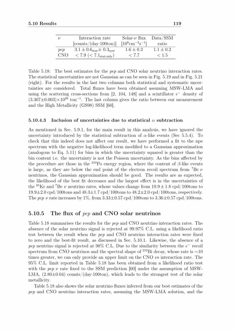
5.10 Results 119
ν Interaction rate Solar-ν flux Data/SSM[counts/(day·100ton)] [108cm−2s−1] ratio
pep 3.1± 0.6stat± 0.3syst 1.6± 0.3 1.1± 0.2CNO < 7.9 (< 7.1stat only) < 7.7 < 1.5
Table 5.18: The best estimates for the pep and CNO solar neutrino interaction rates.The statistical uncertainties are not Gaussian as can be seen in Fig. 5.19 and in Fig. 5.21(right). For the results in the last two columns both statistical and systematic uncer-tainties are considered. Total fluxes have been obtained assuming MSW-LMA andusing the scattering cross-sections from [2, 104, 148] and a scintillator e− density of(3.307±0.003)×1029 ton−1. The last column gives the ratio between our measurementand the High Metallicity (GS98) SSM [60].
5.10.4.3 Inclusion of uncertainties due to statistical α subtraction
As mentioned in Sec. 5.9.1, for the main result in this analysis, we have ignored theuncertainty introduced by the statistical subtraction of α-like events (Sec 5.5.4). Tocheck that this indeed does not affect our result, we have performed a fit to the npespectrum with the negative log-likelihood term modified to a Gaussian approximation(analogous to Eq. 5.11) for bins in which the uncertainty squared is greater than thebin content i.e. the uncertainty is not the Poisson uncertainty. As the bins affected bythe procedure are those in the 210Po energy region, where the content of β-like eventsis large, as they are below the end point of the electron recoil spectrum from 7Be νneutrinos, the Gaussian approximation should be good. The results are as expected,the likelihood of the best fit decreases and the largest effect is in the uncertainties ofthe 85Kr and 7Be ν neutrino rates, whose values change from 19.9± 1.8 cpd/100tons to19.9±2.0 cpd/100tons and 48.3±1.7 cpd/100tons to 48.2±2.0 cpd/100tons, respectively.The pep ν rate increases by 1%, from 3.33±0.57 cpd/100tons to 3.36±0.57 cpd/100tons.
5.10.5 The flux of pep and CNO solar neutrinos
Table 5.18 summarises the results for the pep and CNO neutrino interaction rates. Theabsence of the solar neutrino signal is rejected at 99.97% C.L. using a likelihood ratiotest between the result when the pep and CNO neutrino interaction rates were fixedto zero and the best-fit result, as discussed in Sec. 5.10.1. Likewise, the absence of apep neutrino signal is rejected at 98% C.L. Due to the similarity between the e− recoilspectrum from CNO neutrinos and the spectral shape of 210Bi decay, whose rate is ∼10times greater, we can only provide an upper limit on the CNO νs interaction rate. The95% C.L. limit reported in Table 5.18 has been obtained from a likelihood ratio testwith the pep ν rate fixed to the SSM prediction [60] under the assumption of MSW-LMA, (2.80±0.04) counts/(day·100ton), which leads to the strongest test of the solarmetallicity.
Table 5.18 also shows the solar neutrino fluxes inferred from our best estimates of thepep and CNO neutrino interaction rates, assuming the MSW-LMA solution, and the

120Measurement of the pep and CNO solar neutrino interaction rates
in Borexino
[MeV]νE
-110 1 10
survival probability
eν:
ee
P
0
0.1
0.2
0.3
0.4
0.5
0.6
0.7
0.8
0.9
1
pp - All solarBe - Borexino7
pep - BorexinoB - SNO LETA + Borexino8
B - SNO + SK8
MSW-LMA Prediction
Figure 5.25: Electron neutrino survival probability (Pee) as a function of energy. Thered line corresponds to the measurement presented in this PhD thesis. The pp and 7Bemeasurements of Pee given in [25] are also shown. The 8B ν measurements of Pee wereobtained from [21, 24, 81], as indicated in the legend. The MSW-LMA prediction bandis the 1σ range of the mixing parameters given in [2].
ratio of these values to the High Metallicity (GS98) SSM predictions [60]. Both resultsare consistent with the predicted High and Low Metallicity SSM fluxes assuming MSW-LMA. Under the assumption of no neutrino flavor oscillations, we would expect a pepneutrino interaction rate in Borexino of (4.47±0.05) counts/(day·100ton); the observedinteraction rate disfavours this hypothesis at 97% C.L. If this discrepancy is due to νeoscillation to νµ or ντ we find Pee=0.62±0.17 at 1.44MeV. This result is shown alongsideother solar neutrino Pee measurements and the MSW-LMA prediction in Fig. 5.25.
5.11 Conclusions and outlookWe have achieved the necessary sensitivity to provide, for the first time, evidence of thesignal from pep neutrinos and to place the strongest constraint on the CNO neutrinoflux to date. This has been made possible by the combination of low levels of intrinsicbackground in Borexino and the implementation of novel background discriminationtechniques. The result for the pep neutrino interaction rate does not yet have the suffi-cient precision to disentangle between the Pee predictions of various oscillation models,and the constraint on the CNO neutrino flux cannot yet discern between the High and

5.11 Conclusions and outlook 121
Low Metallicity SSM. However, the success in the reduction of 11C background raisesthe prospect for higher precision measurements of pep and CNO neutrino interactionrates by Borexino after further running, especially if the next dominant background,210Bi, is reduced by scintillator re-purification.

Chapter 6
Conclusions
The Borexino experiment has achieved the necessary sensitivity to provide, for thefirst time, evidence of the rare signal from pep neutrinos and to place the strongestconstraint on the CNO neutrino flux to date. The absence of the pep and CNO solarneutrino interaction is rejected at 99.97% C.L., likewise the absence of a pep neutrinosignal is rejected at 98% C.L. Due to the small statistics sample and the similaritybetween the electron recoil spectrum of CNO solar neutrinos and the spectral shape ofthe internal radioactive contaminant 210Bi whose rate is ∼ 10 times greater, only anupper limit on the CNO interactions could be provided.
The rate of the pep solar neutrino interactions in Borexino is 3.1 ± 0.6 (stat) ±0.3 (syst) counts/(day·100ton). Assuming the pep neutrino flux predicted by the So-lar Standard Model, the constraint on the CNO solar neutrino interaction rate is 7.9counts/(day·100ton) at 95% C.L. Assuming the MSW-LMA solution to solar neutrinooscillations, these values correspond to solar neutrino fluxes of (1.6 ± 0.3) ×108 cm−2s−1
and 7.7 ×108 cm−2s−1, respectively, in agreement with both High and Low Metallic-ity Standard Solar Models. These results represent the first direct evidence of the pepneutrino signal and the strongest constraint of the CNO solar neutrino flux to date.
Under the assumption of no neutrino flavor oscillations, we would expect a pep neu-trino interaction rate in Borexino of (4.47±0.05) counts/(day·100ton); the observedinteraction rate disfavours this hypothesis at 97% C.L. If this discrepancy is due to νeoscillation to νµ or ντ we find Pee=0.62±0.17 at 1.44MeV.


Bibliography
[1] G. Bellini et al. First evidence of pep solar neutrinos by direct detection in Borex-ino. Phys. Rev. Lett., 108:051302, 2012. III, 4, 31, 35
[2] K. Nakamura et al. The Review of Particle Physics. J. Phys. G., 37:075021, 2010.1, 3, 5, 6, 10, 11, 13, 35, 70, 95, 100, 119, 120
[3] C.L. Cowan, F.B. Reines, H.W. Kruse, and A.D. McGuire. Detection of the FreeNeutrino: a Confirmation. Science, 124:103–104, 1956. 1
[4] G. Danby et al. Final tau-neutrino results from the DONuT experiment. Phys.Rev. D, 78:052002, 2008. 1, 2
[5] K. Kodama et al. Observation of High-Energy Neutrino Reactions and the Exis-tence of Two Kinds of Neutrinos. Phys. Rev. Lett., 9:36–44, 1962. 1
[6] John N. Bahcall. Neutrino Astrophysics. Cambrige University Press, 1989. 1, 15,16, 17, 18, 20, 22, 23
[7] Lawrence M. Krauss, Sheldon L. Glashow, and David N. Schramm. Antineutrinoastronomy and geophysics. Nature, 310:191–198, 1984. 2
[8] Thomas K. Gaisser. Cosmic rays and particle physics. Cambrige University Press,1990. 2
[9] K.S. Hirata et al. Observation of a neutrino burst from the supernova SN1987A.Phys. Rev. Lett., 58:1490, 1987. 2
[10] M. Malek et al. Search for Supernova Relic Neutrinos at Super-Kamiokande.Phys. Rev. Lett., 90:061101, Feb 2003. 2
[11] K. Schreckenbach, G. Colvin, W. Gelletly, and F. Von Feilitzsch. Determinationof the Anti-Neutrino Spectrum from U-235 Thermal Neutron Fission Products upto 9.5-MeV. Phys. Lett., B160:325–330, 1985. 2
[12] A. A. Hahn et al. Anti-Neutrino Spectra from Pu-241 and Pu-239 Thermal Neu-tron Fission Products. Phys. Lett., B218:365–368, 1989. 2
[13] B. Pontecorvo. Neutrino Experiments and the Problem of Conservation of Lep-tonic Charge. Sov. Phys. JETP, 26:984–988, 1968. 4

126 BIBLIOGRAPHY
[14] B.T. Cleveland et al. Measurement of the Solar Electron Neutrino Flux with theHomestake Chlorine Detector. Astrophys. J., 496:505, 1988. 4, 22
[15] Y. Fukuda et al. Solar Neutrino Data Covering Solar Cycle 22. Phys. Rev. Lett.,77:1683, 1996. 4
[16] P. Anselmann et al. Solar neutrinos observed by GALLEX at Gran Sasso. Phys.Lett., B285:376–389, 1992. 4, 26
[17] W. Hampel et al. GALLEX solar neutrino observations: Results for GALLEXIV. Phys. Lett. B, 447:127, 1999. 4, 26
[18] M. Altman et al. Complete results for five years of GNO solar neutrino observa-tions. Phys. Lett. B, 616:174, 2005. 4, 26
[19] A. Abdurashitov et al. Measurement of the solar neutrino capture rate withGallium metal, Part III. Phys. Rev. C, 80:015807, 2009. 4, 26
[20] S. Fukuda et al. Determination of solar neutrino oscillation parameters using 1496days of Super-Kamiokande I data. Phys. Lett. B, 539:179–187, 2002. 4
[21] J. P. Cravens et al. Solar neutrino measurements in Super-Kamiokande-II. Phys.Rev. D, 78:032002, Aug 2008. 4, 27, 120
[22] Q.R. Ahmad et al. Measurement of the Rate of νe + d→ p+ p+ e− InteractionsProduced by 8B Solar Neutrinos at the Sudbury Neutrino Observatory. Phys.Rev. Lett., 87:071301, 2001. 4, 15, 22, 27, 28
[23] Q.R. Ahmad et al. Direct Evidence for Neutrino Flavor Transformation fromNeutral-Current Interactions in the Sudbury Neutrino Observatory. Phys. Rev.Lett., 89:011301, 2002. 4, 15, 22, 27, 28
[24] B. Aharmim et al. Low Energy Threshold Analysis of the Phase I and Phase IIData Sets of the Sudbury Neutrino Observatory. Phys. Rev. C, 81:055504, 2010.4, 120
[25] G. Bellini et al. Precision Measurement of the 7Be Solar Neutrino InteractionRate in Borexino. Phys. Rev. Lett., 107:141302, Sep 2011. 4, 21, 27, 31, 35, 36,42, 43, 55, 57, 60, 67, 69, 71, 72, 73, 79, 82, 99, 100, 103, 104, 113, 115, 117, 118,120
[26] G. Bellini et al. Absence of a day-night asymmetry in the 7Be solar neutrino ratein Borexino. Phys. Lett. B, 707:22–26, 2012. 4, 25, 28, 31, 35
[27] Y. Fukuda et al. Evidence for Oscillation of Atmospheric Neutrinos. Phys. Rev.Lett., 81:1562, 1998. 4
[28] Y. Ashie et al. Evidence for an Oscillatory Signature in Atmospheric NeutrinoOscillations. Phys. Rev. Lett., 93:101801, 2004. 4
BIBLIOGRAPHY 127
[29] K. Eguchi et al. First Results from KamLAND: Evidence for Reactor Anti-Neutrino Disappearance. Phys. Rev. Lett., 90:021802, 2003. 4, 28
[30] T. Araki et al. Measurement of Neutrino Oscillation with KamLAND: Evidenceof Spectral Distortion. Phys. Rev. Lett., 94:081801, 2005. 4
[31] S. Abe et al. Precision Measurement of Neutrino Oscillation Parameters withKamLAND. Phys. Rev. Lett, 100:221803, 2008. 4, 13
[32] Y. Abe et al. Indication for the disappearance of reactor electron antineutrinosin the Double Chooz experiment. arXiv:1112.6353 [hep-ph], 2011. 4, 12
[33] M.H. Ahn et al. Measurement of neutrino oscillation by the K2K experiment.Phys. Rev. D, 74:072003, 2006. 4
[34] D.G. Micheal et al. Observation of Muon Neutrino Disappearance with the MI-NOS Detectors in the NuMI Neutrino Beam. Phys. Rev. Lett., 97:191801, 2006.4
[35] P. Adamson et al. Measurement of Neutrino Oscillations with the MINOS Detec-tors in the NuMI Beam. Phys. Rev. Lett., 101:131802, 2008. 4
[36] P. Adamson et al. Improved search for muon-neutrino to electron-neutrino oscil-lations in MINOS. Phys. Rev. Lett, 107:181802, 2011. 4, 12
[37] N. Agafonova et al. Observation of a first ντ candidate in the OPERA experimentin the CNGS beam. Phys. Lett. B, 691:138, 2010. 4
[38] K. Abe et al. Indication of Electron Neutrino Appearance from an Accelerator-Produced Off-Axis Muon Neutrino Beam. Phys. Rev. Lett., 107:041801, 2011. 4,12
[39] G. Pontecorvo. Mesonium and anti-mesonium. Sov. Phys. JETP, 6:429, 1957. 4,5
[40] Z. Maki, M. Nakagawa, and S. Sakata. Remarks on the unified model of elementaryparticles. Prog. Theor. Phys., 28:870, 1962. 4, 5
[41] L. Wolfenstein. Neutrino oscillations in matter. Phys. Rev. D, 107:2369, 1978. 5,6, 8, 9, 24, 28
[42] S. Mikheev and A.Y. Smirnov. Resonance enhancement of oscillations in matterand solar neutrino spectroscopy. Sov. J. Nucl. Phys, 42:913, 1985. 5, 6, 9, 24, 25,28
[43] E.Kh. Akhmedov and A.Y. Smirnov. Paradoxes of neutrino oscillations. Phys.Atom. Nucl., 72:1363, 2009. 5
[44] V. Gribov and B. Pontecorvo. Neutrino astronomy and lepton charge. Phys. Lett.B, 28:493, 1969. 7

128 BIBLIOGRAPHY
[45] V. Barger et al. Matter effects on three-neutrino oscillations. Phys. Lett. D,22:2718, 1980. 8, 9
[46] P. Langacker et al. On the Mikheyev-Smirnov-Wolfenstein (MSW) Mechanism ofAmplification of Neutrino Oscillations in Matter. Nucl. Phys. B, 282:589, 1987.10
[47] A. Aguilar et al. Evidence for neutrino oscillations from the observation of anti-neutrino(electron) appearance in a anti-neutrino(muon) beam. Phys. Rev. D,64:112007, 2001. 10
[48] A.A. Aguilar-Arevalo et al. Search for Electron Neutrino Appearance at the∆m2 ∼ 1 eV2 Scale. Phys. Rev. Lett., 98:231801, 2007. 10
[49] The ALEPH Collaboration, The DELPHI Collaboration, The L3 Collaboration,The OPAL Collaboration, The SLD Collaboration, The LEP Electroweak Work-ing Group, and The SLD Electroweak and Heavy Flavour Groups. Precision elec-troweak measurements on the Z resonance. Physics Report, 427:257–454, 2006.10
[50] F. Boehm et al. Final results from the Palo Verde neutrino oscillation experiment.Phys. Rev. D, 64:112001, 2001. 12
[51] M. Apollonio et al. Search for neutrino oscillations on a long base-line at theCHOOZ nuclear power station. Eur. Phys. J. C, 27:331–374, 2003. 12
[52] The Daya Bay Collaboration. A Precision Measurement of the Neutrino MixingAngle theta_13 using Reactor Antineutrinos at Daya Bay. arXiv:0701029 [hep-ph], 2007. 12
[53] J.K. Ahn et al. RENO: An Experiment for Neutrino Oscillation Parametertheta_13 Using Reactor Neutrinos at Yonggwang. arXiv:1003.1391[hep-ph], 2010.12
[54] S.M. Bilenky and S.T. Petcov. Massive neutrinos and neutrino oscillations. Rev.Mod. Phys, 59:671, 1987. 13
[55] R. Davis, D.S. Harmer, and K.C. Hoffman. Search for Neutrinos from the Sun.Phys. Rev. Lett., 20:1205, 1968. 15, 22, 26
[56] Raymond Davis. Solar Neutrinos. II. Experimental. Phys. Rev. Lett., 12:303–305,Mar 1964. 15
[57] J.N. Bahcall, A.M. Serenelli, and S Basu. New Solar Opacities, Abundances,Helioseismology and Neutrino Fluxes. Astrophys. J. Suppl., 621:L85, 2005. 17,19, 28
[58] J.N. Bahcall, A.M. Serenelli, and S Basu. 10,000 Standard Solar Models: A MonteCarlo Simulation. Astrophys. J. Supp., 165:400, 2006. 17, 23, 68, 70

BIBLIOGRAPHY 129
[59] C. Pena-Garay and A.M. Serenelli. Solar neutrinos and the solar compositionproblem. arXiv: 0811.2424[astro-ph], accepted for publication on PRL, 2008. 17,18, 35
[60] A. Serenelli, W. Haxton, and C. Peña-Garay. Solar models with accretion. I.Application to the solar abundance problem. The Astrophysical Journal, 743:24,2011. 17, 18, 20, 68, 69, 70, 72, 98, 104, 118, 119, 120
[61] N. Grevesse and A.J. Sauval. Standard Solar Composition. Space Sci. Rev.,85:161, 1998. 17
[62] M. Asplund, N. Grevesse, and A. J. Sauval. The Solar Chemical Composition.ASP Conference Series, 336:25, 2005. 17, 18
[63] M. Asplund, N. Grevesse, A. J. Sauval, and P. Scott. New solar composition: theproblem with solar models revisited. The Astrophysical Journal Letters, 705:123,2009. 17, 18
[64] S. Basu. The Solar Metallicity Problem: What is the Solution? In Proc. GONG2008/SOHO XXI Solar-stellar dynamos as revealed by helio and asteroseismology,volume 416, page 193, 2009. 17, 18
[65] C. Allende Prieto and D. Lambert. The Forbidden abundance of oxygen in theSun. Astrophys. J., 556:L63–L66, 2001. 17
[66] C. Allende Prieto and D. Lambert. A reapprisal of the solar photospheric C/Oratio. Astrophys. J., 573:L137–L140, 2002. 17
[67] M. Asplund, N. Grevesse, A. J. Sauval, C. Allende Prieto, and D. Kiselman. Lineformation in solar granulation. IV. [O I], O I and OH lines and the photosphericO abundance. Astronomy and Astrophysics, 417:751–768, 2004. 17
[68] M. Asplund, N. Grevesse, A. J. Sauval, C. Allende Prieto, and R. Blomme. Lineformation in solar granulation. VI. [C I], C I, CH and C2 lines and the photosphericC abundance. Astronomy and Astrophysics, 431:693–705, 2005. 17
[69] M. Asplund. Line formation in solar granulation. III. The photospheric Si andmeteoritic Fe abundances. Astronomy and Astrophysics, 359:755–758, 2000. 17
[70] John N. Bahcall. The luminosity constraint on solar neutrino fluxes. Phys. Rev.C, 65:025801, 2002. 20
[71] C. Casella et al. First Measurement of the d(p,γ)3He cross section down to thesolar Gamow peak. Nucl. Phys. A, 706:203–216, 2002. 21
[72] M. Junker et al. Cross section of 3He(3He,2p)4He measured at solar energies.Phys. Rev. C, 57:2700–2710, May 1998. 21
[73] R. Bonetti et al. First Measurement of the 3He(3He,2p)4He Cross Section downto the Lower Edge of the Solar Gamow Peak. Phys. Rev. Lett., 82:5205–5208, Jun1999. 21

130 BIBLIOGRAPHY
[74] D. Bemmerer et al. Activation Measurement of the 3He(α,γ)7Be Cross Section atLow Energy. Phys. Rev. Lett., 97:122502, Sep 2006. 21
[75] H. Costantini et al. The 3He(α,γ)7Be S-factor at solar energies: The prompt γexperiment at LUNA. Nucl. Phys. A, 814:144–158, 2008. 21
[76] Y. Fukuda et al. Solar 8B and hep Neutrino Measurements from 1258 Days ofSuper-Kamiokande Data. Phys. Rev. Lett., 86:5651, 2001. 21, 28
[77] The Borexino Collaboration. Direct Measurement of the 7Be Solar Neutrino Fluxwith 192 Days of Borexino Data. Phys. Rev. Lett., 101:091302, 2008. 21, 27, 43,57
[78] C. Arpesella et al. First real time detection of 7Be solar neutrinos by Borexino.Phys. Lett., B658:101–108, 2008. 21, 27, 57
[79] B. Aharmim et al. Electron energy spectra, fluxes, and day-night asymmetriesof 8B solar neutrinos from measurements with NaCl dissolved in the heavy-waterdetector at the Sudbury Neutrino Observatory. Phys. Rev. C, 72:055502, 2005.22, 27, 28
[80] B. Aharmim et al. An Independent Measurement of the Total Active 8B SolarNeutrino Flux Using an Array of 3He Proportional Counters at the SudburyNeutrino Observatory. Phys. Rev. Lett., 101:111301, 2008. 22, 27
[81] G. Bellini et al. Measurement of the solar 8B neutrino rate with a liquid scintil-lator target and 3 Mev energy threshold in the Borexino detector. Phys. Rev. D,82:033006, Aug 2010. 22, 27, 31, 35, 73, 74, 120
[82] A. Formicola et al. Astrophysical S-factor of 14N(p,γ)15O. Phys. Lett. B, 591:61–68, 2008. 23
[83] M. Marta et al. The 14N(p,γ)15O reaction studied with a composite germaniumdetector. Phys. Rev. C, 83:045804, Apr 2011. 23
[84] P. J. LeBlanc et al. Constraining the S factor of 15N(p,γ)16O at astrophysicalenergies. Phys. Rev. C, 82:055804, Nov 2010. 23
[85] S.T. Petcov. Analytic treatment of high-order adiabatic approximations of two-neutrino oscillations in matter. Phys. Lett. B, 200:373, 1988. 24
[86] M. Bruggen, Haxton W.C., and Quian Y.Z. Landau-zener treatments of solarneutrino oscillations. Phys. Rev. D, 51:4028, 1995. 24, 25
[87] A.Yu Smirnov and S.P. Mikheev. Neutrino Oscillations In Matter With Vary-ing Density. In Proc. of the VIth Moriond Workshop on Massive Neutrinos inAstrophysics and Particle Physics, page 355, 1986. 24
[88] S. Toshev. Exact analytical solution of the two-neutrino evolution equation inmatter with exponentially varying density. Phys. Lett. B, 196:170, 1987. 24
BIBLIOGRAPHY 131
[89] S.T. Petcov. Exact analytic description of neutrino oscillations in matter with anexponentially varying density for an arbitrary number of neutrino species. Phys.Lett. B, 214:259, 1988. 25
[90] S.P. Mikheev and A.Y. Smirnov. 3 ν oscillations in matter and solar neutrinodata. Phys. Lett. B, 200:560, 1987. 25
[91] G. Pontecorvo. report PD-205. Technical report, Chalk River Lab., 1946. 26
[92] A.I. Abazov et al. Search for neutrinos from sun using the reaction Ga-71(electron-neutrino e-) Ge-71. Phys. Rev. Lett., 67:3332, 1991. 26
[93] K.S. Hirata et al. Observation of 8B solar neutrinos in the Kamiokande-II detector.Phys. Rev. Lett., 63:16, 1989. 27
[94] Y. Fukuda et al. Measurements of the Solar Neutrino Flux from Super-Kamiokande’s First 300 Days. Phys. Rev. Lett., 81:1158, 1998. 27
[95] J. Hosaka et al. Solar neutrino measurements in Super-Kamiokande-I. Phys. Rev.D, 73:112001, 2006. 27
[96] G. Alimonti et al. The Borexino detector at the Laboratori Nazionali del GranSasso. Nucl. Instr. and Meth. A, 600:568–593, 2009. 27, 31, 35, 36, 37, 53, 63, 71
[97] John N. Bahcall, M.C. Gonzalez-Garcia, and C. Pena-Garay. Solar neutrinosbefore and after KamLAND. JHEP, 02:009, 2003. 28
[98] B. Aharmin et al. Combined Analysis of all Three Phases of Solar Neutrino Datafrom the Sudbury Neutrino Observatory. arXiv: 1109.0763[hep-ph], 2011. 28, 29
[99] G. Bellini et al. Study of solar and other unknown anti-neutrino fluxes withBorexino at LNGS. Phys. Lett. B, 696:191–196, 2011. 31
[100] G. Bellini et al. Observation of Geo-Neutrinos. Phys. Lett. B, 687:299–304, 2010.31, 72, 73, 75
[101] G. Bellini et al. New experimental limits on the Pauli-forbidden transitions in12C nuclei obtained with 485 days Borexino data. Phys. Rev. C, 81:034317, Mar2010. 31
[102] G. Alimonti et al. Ultra-low background measurements in a large volume under-ground detector. Astropart. Phys., 8:141–157, 1998. 32
[103] G. Alimonti et al. A large-scale low-background liquid scintillation detector: thecounting test facility at Gran Sasso. Nucl. Instr. and Meth. A, 406:411–426, 1998.32
[104] John N. Bahcall. Solar neutrinos: Radiative corrections in neutrino-electron scat-tering experiments. Phys. Rev. D, 51:6151–6158, 1995. 34, 100, 119
132 BIBLIOGRAPHY
[105] G. Bellini et al. Muon and Cosmogenic Neutron Detection in Borexino. JINST,6:P05005, 2011. 35, 36, 59, 75, 82
[106] G. Alimonti et al. Science and technology of Borexino: a real-time detector forlow energy solar neutrinos. Astropart. Phys., 16:205–234, 2002. 35, 36
[107] J. Benzinger et al. A Scintillator Purification System for the Borexino SolarNeutrino Detector. Nucl. Instr. and Meth. A, 587:277–291, 2008. 35, 36, 73
[108] G. Alimonti et al. The liquid handling systems for the Borexino solar neutrinodetector. Nucl. Instr. and Meth. A, 609:58–78, 2009. 35, 36
[109] F. Elisei et al. Measurments of liquid scintillator properties for the borexinodetector. Nucl. Instr. Met. A, 400:53–68, 1997. 35, 37, 51
[110] M. Chen et al. Quenching of undesired fluorescence in a liquid scintillator particledetector. Nucl. Instr. and Meth. A, 420:189–201, 1999. 35
[111] G. Alimonti et al. Light propagation in a large volume liquid scintillator. Nucl.Instr. and Meth. A, 440:360–371, 2000. 35, 37, 52
[112] J. Benizinger et al. The nylon scintillator containment vessels for the Borexinosolar neutrino experiment. Nucl. Instr. and Meth. A, 582:509–534, 2007. 35, 76
[113] A. Ianni et al. The Measurements of 2200 ETL9351 type photomultipliers forthe Borexino experiment with the photomultiplier testing facility at LNGS. Nucl.Instr. and Meth. A, 537:683–697, 2005. 35, 52
[114] A. Brigatti et al. The Photomultiplier tube testing facility for the Borexino ex-periment at LNGS. Nucl. Instr. and Meth. A, 537:521, 2005. 35
[115] J.B. Birks. Photophysics of Aromatic Molecules. Wiley-Interscience, 1970. 37, 38,50
[116] H.O. Back et al. Pulse-Shape discrimination with the Counting Test Facility.Nucl. Instr. and Meth. A, 584:98–113, 2008. 39
[117] E. Gatti and F. De Martini. A New Linear Method of Discrimination betweenElementary Particles in Scintillation Counters. Nuclear Electronics, 2:265–276,1962. 39, 40
[118] Stefano Perasso. Monte Carlo based measurement of the 7Be solar neutrino fluxin Borexino. PhD thesis, Università degli Studi di Genova, 2010. 40, 84, 99
[119] Richard Saldanha. Precision measurement of the 7Be Solar Neutrino InteractionRate in Borexino. PhD thesis, Princeton University, January 2012. 40, 78, 84,99, 100, 102, 113, 115, 118
[120] Y. Kino et al. Positron Annihilation in Liquid Scintillator for Electron Antineu-trino Detection. Jour. Nucl. Radiochem. Sci., 1:63, 200. 40, 48

BIBLIOGRAPHY 133
[121] D. Franco et al. Positronium signature in organic liquid scintillators for neutrinoexperiments. Phys. Rev. C, 83:015504, 2011. 41, 48, 87, 88, 89
[122] G. Alimonti et al. Measurement of the 14C abundance in a low-background liquidscintillator. Nucl. Instr. Meth. A, 406:411–426, 1998. 42
[123] C. Galbiati et al. Cosmogenic 11C production and sensitivity of organic scintillatordetectors to pep and CNO neutrinos. Phys. Rev. C, 71:055805, 2005. 42, 81
[124] Werner Maneschg. Low-energy solar neutrino spectroscopy with Borexino : To-wards the detection of the solar pep and CNO neutrino flux. PhD thesis, MPI fuerKernphysik, May 2011. 45, 55, 93
[125] W. Maneschg et al. Production and characterization of a custom-made 228Thsource with reduced neutron source strength for the Borexino experiment.arXiv:1110.1217[physics.ins-det], 2011. 45, 55, 93
[126] A. Agostinelli et al. GEANT4 – a simulation toolkit. Nucl. Instr. Meth. A,506:250–303, 2003. 47
[127] John Bahcall. John Bahcall website http://www.sns.ias.edu/~jnb/ , 2005. 48
[128] P.C. de Holanda et al. Toward precision measurements in solar neutrinos.arXiv:0404042v3 [hep-ph], 2004. 48, 100
[129] J.K. Tuli. Evaluated Nuclear Structure Data File. Technical report, BrookhavenNational Laboratory, April 1987. 48
[130] W. Maneschg. Comparison of the particle generators and rdm/snu in the Borexinosimulation package G4bx. Borexino Internal Memo, 2010. 48, 100
[131] F. Rohrlich and B.C. Carlson. Positron-Electron Difference in Energy Loss andMultiple Scattering. Phys. Rev., 93:38, 1954. 51
[132] H. Gumus. New stopping power formula for intermediate energy electrons. Appl.Radiat. Isot., 66:1886–1890, 2008. 51
[133] L. Oberauer, C. Grieb, F. von Feilitzsch, and I. Manno. Light concentrators forBorexino and CTF. Nucl. Instr. and Meth. A, 530:453–462, 2004. 52
[134] Steven E. Hardy. Measuring the 7Be Neutrino Flux From the Sun: Calibration ofthe Borexino Solar Neutrino Detector. PhD thesis, Virginia Polytechnic Instituteand State University, March 2010. 55, 57, 58
[135] O.Ju Smirnov. An approximation of the ideal scintillation detector line shape witha generalized gamma distribution. Nucl. Instr. and Meth., 595:410–418, 2008. 61
[136] S. Abe et al. Study of the Production of Radioactive Isotopes through CosmicMuon Spallation in KamLAND. Phys. Rev. C, 81:025807, 2010. 74

134 BIBLIOGRAPHY
[137] C. Arpesella et al. Measurements of extremely low radioactivity levels in BOREX-INO. Astropart. Phys., 18:1–25, 2002. 76, 93, 103
[138] Margherita Buizza Avanzini. The 8B Solar Neutrino Analysis in Borexino andSimulations of Muon Interaction Products in Borexino and Double Chooz. PhDthesis, Università degli Studi di Milano, 2011. 76
[139] B. Caccianiga et al. Minutes of the Meetings. Internal Memo of the Borexino 7BeCuts Committee, 2010. 77, 78
[140] M. Deutsh. Proposal for a Cosmic Ray Detection System for the Borexino SolarNeutrino Experiment. Technical report, Massachussetts Institute of Technology,1996. 82
[141] H.O. Back et al. CNO and pep neutrino spectroscopy in Borexino: Measure-ment of the deep-underground production of cosmogenic 11C in an organic liquidscintillator. Phys. Rev. C, 74:045805, 2006. 82
[142] A. Hoecker and others. TMVA 4 Toolkit for Multivariate Data Analysis withROOT Users Guide http://tmva.sourceforge.net/docu/TMVAUsersGuide.pdf , nov 2009. 88
[143] R. Brun and others. ROOT: A Data Analysis Framework http://root.cern.ch ,jun 2011. 88, 106
[144] E. Plassmann and Langer L. Das β-Spektrum Des RaE. Nucl. Phys., 31:293,1962. 100, 117
[145] E. Plassmann and Langer L. Beta Spectrum of Radium E. Phys. Rev., 96:6, 1954.117
[146] A. Grau Charles and Grau Malonda A. Precision measurement of the RaE shapefactor. Nucl. Phys. A, 596:83, 1996. 117
[147] A. Grau Charles. Beta shapefactor determinations by the cutoff energy yieldmethod. Nucl. Instr. Meth. A, 551:312, 2005. 117
[148] J. Erler and M.J. Ramsey-Musolf. The Weak Mixing Angle at Low Energies.Phys. Rev. D, 72:073003, 2005. 119

Acknowledgements
Un gran numero di persone meritano una menzione di ringraziamento; alcune hannocontribuito significativamente a questo importante risultato, altre mi hanno sostenutoo mi hanno aiutato, altre ancora hanno avuto un importante ruolo nei miei anni dadottorando.
Una menzione particolare è per il mio relatore, Marco Pallavicini. Marco è un fisicoda Serie A e i suoi insegnamenti, sia diretti che indiretti, sono davvero preziosi e mihanno aiutato a crescere come fisico. O almeno, questa è la mia opinione.
Un ringraziamento dal profondo dell’animo va alla nostra imperatrice Gemma Testera.Con Gemma ho lavorato davvero bene e mi sono divertito parecchio. Gemma è piena diqualità che la rendono eccezionale come donna e come fisica, e lavorare fianco a fiancocon lei mi ha aiutato a sviluppare le mie abilità da fisico.
Special thanks to the members of the Borexino pep dream team which I so proudlybelong.
To Alvaro, one of the brighter physicist I have ever met. Without Alvaro the resultof the pep analysis would be extremely less significant. Those days in June and July,when we made this analysis converge, were extremely tough. However, I bring with mean extremely good memory of those days. The satisfaction for the accomplishment ofthe analysis, carried out on that sleepless night before the General Meeting, is going tobe one of the greatest emotions in my career as a physicist.
To Richard, because it is easy to work with Richard, and his knowledge and skill areextremely precious. The help you gave us with the fitter is priceless.
A Davide, perché con Davide lavoro sempre molto bene, ed è sempre un piacerechiacchierare con lui. Mi sono divertito parecchio nelle pep week e le varie volte che ab-biamo collaborato a Genova, Milano o Gran Sasso. Sono felice che questa collaborazionecontinuerà nella mia prossima avventura in Dark Side.
Ad Alessandro, perché é un mostro di bravura e di competenza, e mi consiglia spessoletture interessanti. Si impara sempre qualcosa da Alessandro, anche solo per osmosi.Mi sono divertito nei periodi al Gran Sasso, e spero sarà così anche in futuro.
A Margherita, perché é un’ottima fisica e una vera donna. La tua abilità nel simularequalsiasi cosa in qualsiasi situazione e impiegando una frazione di tempo trascurabileis really amazing. Purtroppo la nostra collaborazione si fermerà, almeno per qualcheanno, ma auguro a te e alla piccola Elicottera tutta la serenità e la gioia che vi meritate.
And finally to the Dark Lord Cristiano, Commander in Chief of the pep workinggroup and external advisor of my thesis. Cristiano is a skilled politician and manager.
His management of the pep working group was outstanding.
I want to thank a large number of people within the Borexino collaboration.Livia, mi diverto sempre con te, nonostante i miei occhi siano in costante pericolo ogni
volta che sei nelle vicinanze. Lavorare con te è stato piacevole, ed è stato molto piacevoleseguire insieme la scuola estiva a Varenna. Magari un giorno davvero riusciremo ariscrivere la RunValidation macro.
Sandra, i lunghissimi viaggi Arenzano – Genova sarebbero stati interminabili senzadi te.
George, the God of Electronics. Thanks for the constant help during my months asRun Coordinator.
Pablo, porque la pasión de la noche está caliente como una espada de fuego.Amanda, because she brings happiness to the cold winter days in Assergi, and because
she has an amazing superpower.Yusuke, arigato gozaimasu. Kaizoku oni ore wa naru.Alex, for his very useful comments about the pep and CNO analysis and the paper.Tizio, Caio e Sempronio per l’aiuto costante durante questi anni.
Un ringraziamento alle persone a Genova che mi piace incrociare nei corridoi o neirispettivi uffici.
Marco B, fisico teorico di rara qualità e calcolatore umano spesso più affidabile diMathematica. Chiacchierare con Marco è sempre un piacere, e spero che un giorno inostri percorsi convergano nuovamente alla stessa Università.
Sara B (che non è di Genova, ma è isomorfa a Genova grazie a Marco), anche se lepiace troppo la statistica Bayesiana.
Giulia perché sei sempre un faro di riferimento, e hai svolto tutta la burocrazia perquesta tesi al posto mio.
Giovanni (Ridolfi) per avermi insegnato quello che so sulla teoria quantistica deicampi e la rinormalizzazione, e per aver letto i capitoli introduttivi di questa tesi.
Gabriele Filipelli e la sua crew, per tutte le chiacchierate quando giravo per il dipar-timento in cerca di ispirazione (o mentre attendevo i risultati di qualche simulazione), eper la stima che mi dimostrate quando mi chiedete opinioni o delucidazioni su qualsiasiargomento inerente alla fisica.
Alessio e Guido, che hanno spesso buoni consigli da elargire.Quello lì, quella là e quegli altri perché è bello incontrare facce familiari al DiFi.
Special thanks to Son Goku, because he always protect our planet from evil menaceslike Saiyans, Freezer, Cell, and Majin Bu. Also, many thanks to Eiichiro Oda becauseevery week I can read a new amazing chapter of One Piece.
Alcune persone speciali che meritano un ringraziamento particolare.Mamma e Papà, perché altrimenti non esisterei, e il mio Zio.Francesca, è stato bello essere il relatore della tua tesi. Mi dispiace che non sarai una
dottoranda in Borexino, ma sono felice che che continuerai a frequentare i Laboratorinella tua nuova avventura lunare.

Carlotta, per aver reso più piacevoli i lunghi inverni Abruzzesi, la lontana fuga a NewYork e la calda estate Spagnola.
Marzia, la mia gemellina. E’ bello capirci al volo e grazie per tutte le volte che mihai ascoltato e tutti i consigli che mi hai dato. Mi raccomando, non fare cazzate.
Irena, la mia sorellina. Penso che tu sia una fisica molto promettente. Mi piacerebbelavorare insieme a te in un futuro. E’ sempre un piacere chiacchierare con te e scam-biarci consigli su qualsiasi cosa. Ricorderò con piacere la fuga da Varenna.
Il ringraziamento più importante è per la mia preziosissima creatura meravigliosa.Hai reso questi tre anni degni di essere vissuti. Sei il Sole che illumina le mie giornate.Grazie per tutte le piccole e grandi cose che condividiamo, per tutte le gioie che riescia regalarmi, per la tua stessa esistenza.


![Cesare Davini and Roberto Paroni - core.ac.uk · 804 C. DAVINI AND R. PARONI oftheCalculusofVariationstoshowhowthemethodstudiedin[18]canbemodified inordertocoverfunctionals of the](https://img.dokumen.tips/doc/110x75/5bdffb7609d3f28f578b9d4b/cesare-davini-and-roberto-paroni-coreacuk-804-c-davini-and-r-paroni-ofthecalculusofvariationstoshowhowthemethodstudiedin18canbemodied.jpg)