Measurement of the decay time of the muon

Garrett WoodsDepartment of Physics

University of California, Davis

2/9/2010

ABSTRACT The purpose of this experiment was to accurately measure the decay time of a muon - using a PMT connected to a scintillator. By capturing 14984 muon decays over 5 days we were able to measure the lifetime to be 2.38 ± 0.04 microseconds using an exponential decay curve fit to our data with a reduced2 of 1.14.

INTRODUCTION:

The main goal of this experiment was to determine, with a high degree of accuracy, the mean lifetime of a muon. The PMT signal to noise ratio (which ensures we were getting the correct signal values), the PMT plateau region (where the PMT's readings don't vary with voltage changes), and time conversion factor of the data acquisition system were also determined.

Muons:

A muon is an elementary particle belonging to the lepton family of particles. Electrons e- , tauons , and three types of neutrinos complete the rest of the leptons. A muon is similar to an electron aside from the fact that it is roughly 200 times as massive, and unlike the electron, it will decay into other forms of matter. The muons which are being measured by this experiment are produced from the influx of cosmic rays which are simply high energy protons emanating from space. As these cosmic rays hit the atmosphere, the particles are broken apart and

new particles are formed from the pieces. The full shower is shown in figure 1.

The current accepted value of the mean lifetime of a muon is approximately 2.2

1

Figure 1: The full decay of a cosmic ray. p-proton, n-neutron, + ,- ,0 - pions, ,- - anti muon and muon, e - , e+ - electron and positron, ν – neutrino, γ – gamma ray.

We are measuring the time between the detection of a -

and the following e - . Image modified with permission, courtesy of wikimedia.

microseconds. As they travel at .98c1, classically these muons would not make it to the ground. In fact they only penetrate the atmosphere about 650 meters before they decay.

d =vt≈650 m (1)

However, once relativity is brought into the equation, these muons have no trouble reaching the ground. When traveling at .98c, an object has a Lorentz factor γ of

v=1

1− v 2

c2

=5.03 (2)

implying that in the frame of an observer on earth, the muon exists for a time of

t=v t0=5.03⋅2.2 s=11.1 s (3)

and can thus make it to the surface without decaying in flight.

Radioactivity:

All radioactive materials undergo radioactive decay. This decay is exponential in nature. A sample of N particles that is likely to decay in a given time interval dt is:

dN =−Ndt (4)

Where is a decay constant. The solution to this differential equation is given by the following function:

N t =N 0 e− t (5)

1 Harris, Randy. Modern Physics (2nd Edition). New York: Addison Wesley, 2007. Pg 18-19. Print.

where N 0 is the number of particles at time zero t=0 and the half-life of the atom (the time in which half of the atoms in the sample will have decayed) is given by

t 1/2=ln 2

(6)

The energy-time uncertainty principle

E tℏ2 (7)

gives the relation between the energy of an objectE and the time that the energy is measured t where ℏ is Planck's constant. Masses in

particle physics are often expressed as energies (related by Einstein's famous equation E=mc2

where m is the mass, and c is the speed of light in a vacuum), and therefore we can estimate the lifetime of the particle by knowing it's mass energy. Therefore, the lifetime of the particle is given by

= ℏ

(8)

where

=G 2 m

5

1923 (9)

where G is the Fermi Coupling Constant which has been experimentally determined elsewhere to be 1.136×10 -5GeV - 2 and m is the mass of the muon in eV. Using equation (8) we were able to estimate the average lifetime of a muon to be 2.3 μs.

The formula for the effective decay time in our experiment (effective decay time is what we were measuring with our setup) is given by

2

1eff

= 1

1capture

(10)

where is the actual decay time of the muon and capture is the time elapsed during the muon's interaction with the 12C nucleus.

EXPERIMENTAL PROCEDURE:

The equipment used is as follows:• RCA-4552 Photomultiplier Tube (PMT)

next to a scintillator tank• Ortec 456J High Voltage Power Supply

(for the PMT)• Time Analyzer Model 2043 (TAC)• Ortec 542 Linear Gate Stretcher

• Ortec 779 Dual Counter• LRS Model 364 4-Fold Logic Gate• LRS Model 222 Dual Gate Generator• Lecroy Model 623B Octal Discriminator• LRS Model 334 Quad Amplifier

General Setup:

We were trying to detect the average decay time of a muon which in effect can be broken down into the time between two events: 1) the muon entering our detector and 2) the detection of the resultant electron from it's decay (shown in figure 1). We are able to detect these events through the use of a plastic scintillator. As the muon travels through the atmosphere, it loses speed as it interacts with the air and (hopefully) by

3

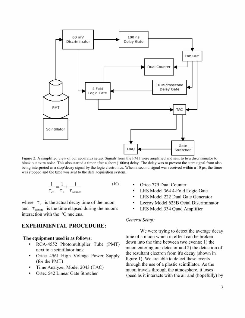
Figure 2: A simplified view of our apparatus setup. Signals from the PMT were amplified and sent to to a discriminator to block out extra noise. This also started a timer after a short (100ns) delay. The delay was to prevent the start signal from also being interpreted as a stop/decay signal by the logic electronics. When a second signal was received within a 10 μs, the timer was stopped and the time was sent to the data acquisition system.

the time it reaches the scintillator it has lost enough energy to stop and eventually decay. Both the muon stopping, and the decay electron will each cause a pulse of light which is detected by the PMT. The time difference between the two events is the decay time of the muon. As both a muon - and an anti-muon + are essentially the same particle (only differing in electrical charge), they both will appear on the instrumentation leading to two possible ways we can observe a signal. A stopped cosmic muon can decay weakly and stimulate the scintillator, or the muon may be absorbed by a nucleus of the scintillator as described by the capture reaction

-Z=Z−1* (11)

where the nucleus gets excited to a higher energy level and emits a photon upon de-excitation which is thus observed.

The source of our muons is purely natural, so we are unable to control the energy or rate of creation. It is possible, however, to estimate a flux using

I =I cos2ddAdt (12)

where I =.0083

cm2⋅s⋅str, is the zenith angle,

dA is the differential area of the detector, andd is the solid angle from which it is possible

to see a muon. As we can expect most come from directly above, we can fix =0 and as no muons are expected to come from below,

d =2 , and dA≈ .02m2 . This gives a rough estimate of 10 muons (with the appropriate energy to be detectable as they decay) passing through the detector each second. As we can only detect about .3 % of these (the muons with energies below 50MeV)2 we can expect to see a flux of about .03 muons per second, or about 2

2 Melissinos, Adrian C. Experiments in modern physics. San Diego: Academic, 2003. Print.

decay events every minute3. This implies that the probability of two muons interacting with our

3 The predicted rates turned out to be somewhat lower than our data suggests. We observed approximately 7 decay events per minute. This may imply a source of error that we haven't accounted for.

4

Figure 3: A diagram of a photomultiplier tube. An incident photon enters the PMT at the bottom of the diagram and is converted into an electron. This electron is pulled towards the first dynode by an electric field. As it strikes the dynode, it kicks out 3 to 4 other electrons which are accelerated towards the next dynode. This process is repeated over the length of the PMT through 14 dynodes such that the number of electrons leaving the PMT is much greater than the number of electrons that entered.

apparatus during the same 10 microsecond window is given by

P n , t = rtn e-rt

n! (13)

where r (.3 muons per second) is the average event rate, t (1x10-6 seconds) is the time interval, and n (2) is the number of events occurring during that time interval. In terms of our apparatus, this yields

P n , t =.3⋅1×10-62 e- .3⋅1×10-6

2! =4.5×10−14 (14)

or approximately 1 in 1 trillion muons will arrive during another muon's 10 microsecond decay window. This effect is incredibly small given the amount of data collected and is therefore ignored completely.4

As the muons enter our apparatus, they are captured by and interact with the scintillator. The

4 With respect to our actual data, we observed 1483612 muons pass through our detector in 4 days yielding an actual probability of approximately 1x10-9.

scintillator is a small tank filled with a substance that is easily excitable. This alone is not specific to scintillators, but rather it is what happens afterwards that which makes them unique. As a particle comes into the scintillator, it excites a valence electron to a higher orbit. As this electron returns to it's previous state5, it is very likely to emit a photon and the properties of the scintillator are such that the emitted photon is allowed to leave the scintillator largely unimpeded. This fluorescence takes place in the average amount of time that it takes an electron to de-excite, approximately 10 ns for our scintillator6.

PMT (Photomultiplier Tube):

The main piece of equipment in our experiment was the PMT. The PMT is similar to a Geiger counter in that it senses the influx of particles, however it amplifies the incoming signal greatly. This is accomplished by the use of dynodes. A dynode is a charged plate inside the PMT that attracts any incoming electrons. When a single electron hits the dynode, it will kick out a larger number of electrons (let's call it N electrons where N outN in ) which are then pulled towards the next dynode. As there are 14 dynodes and N for our PMT is approximately 3.4, we were able to get an amplification factor of

3.414=9×107 (just under 100 billion) from the aperture to the anode.

The detected signals were routed from the PMT to an amplifier, which effectively tripled the signal strength. After our signals were sent through the amplifier, we were getting amplitudes of approximately 500mV for an incident muon and 100mV for a decay signal.

5 It's also possible that the muon may be captured by the nucleus of an atom in the scintillator. This capture process while different from the example above, takes place largely on the same timescale and so we can approximate both processes as taking the same amount of time.

6 Leo, W. R. Techniques for Nuclear and Particle Physics Experiments. 1987. Pg 150-153 Print.

5

Figure 4: A screen capture from the oscilloscope of a decay event. The primary spike (the incident muon) and decay spike (the electron) are apparent above the noise level.

This amplifier was coupled to a discriminator, which acts as a filter to prevent any signals which are below a certain threshold from getting through. This filter allowed us to ignore a significant portion of the noise from the PMT while still allowing our muon signals to pass through so that we wouldn't accumulate a data set comprised of a large number of false decay events.

Whenever a signal amplitude was above the discriminator threshold amplitude (60 mV in this case), it was allowed to pass through to a 100 ns delay gate. The 100 ns delay gate was in place simply to delay the signal from entering the system and prevent it from being seen as both a start and a stop signal by the timer. Once delayed, the signal went to the dual gate generator. This is effectively a timer which was started whenever a pulse was received. The timer put out a constant signal to the coincidence logic gate for as long as it was running. The logic gate simply checks if two things happen at the same time. So as an incident muon's signal was received and the timer

started, if a second signal was received while the timer was still running, the logic was triggered and we knew we had seen a decay and could thus measure the difference in time between the primary and secondary signals with a time analyzer.

The time analyzer (or time amplitude converter / TAC) was triggered anytime a primary signal was seen. The TAC relates the time interval between two events to the amount of charge discharged by a capacitor during this time. When triggered by the start signal, it causes the capacitor to start a voltage ramp. This process is stopped when the logic gate indicates that it has seen a decay signal and the total charge collected forms an output who's height is proportional to the time difference between the start and stop events. The capacitor is then recharged and the system resets. The TAC can then look at the output signal to find the time between the two events.

6

Figure 5: A plot of the average signal to noise ratio of the PMT. The best value is where the ratio is highest at 2400V.

7

Figure 6: A plot of the number of decay counts with respect to voltage. We were trying to find the plateau region, or region where the number of counts does not change (or at least has a minimal change) with respect to a change in the input voltage. This plateau is readily apparent in the range of 2300 - 2500 volts.

Figure 7: Plot of the times in digital units and microseconds. The conversion factor of the unit change is given by the slope of the fit line to be m= 341.41 ± 1.33 DU/μs. We were able to see a linear model fit almost perfectly with a reduced 2 value of .81.

Experiment 1: Determination of the Signal to Noise Ratio of the PMT

In order to accurately measure the lifetime of a muon, we had to first determine the signal to noise ratio of the data that we were getting from the PMT. To do this we took measurements at each 100 volt increment from 2200 V to 2900 V. The lower limit of 2200 volts was chosen due to the fact that it was where we started to see any discernible signal above the level of ambient noise present on the circuit. The upper limit was chosen as it is the highest recommended voltage as per the PMT documentation.

The measurements taken were of the ambient level of noise present and the amplitude of any signal above the noise level occurring within 10 μs of another signal. These secondary pulses are the decay emissions of the muon; the emitted electron shown in figure 4. The level of the decay signals were averaged over a two minute time interval for each 100 volt increment yielding the curve in figure 5.

Experiment 2: Determination of the Plateau Region of the PMT

The PMT has an inherent variation in the number of counts likely to be registered as a function of voltage. We were attempting to find the region in the voltage domain where there was minimal variation (with respect to voltage) in decay counts. This “plateau region” is shown in figure 6.

Experiment 3:Determination of the Conversion Factor from DAQ Digital Units to Seconds

The DAQ we used to measure the time difference between the primary and decay signals did not provide a measurement in seconds, but rather, gave the time in digital units (DUs). We therefore had to determine the conversion factor and/or scaling of the unit change. To do this we ran the delayed output of the dual gate generator

to the oscilloscope and adjusted the output pulses to be round integer values of microseconds as possible. We were then able to plug the output directly into the DAQ to see the values that were being given. For each 1 microsecond we took a 30 second measurement of the DAQ output values. The output was automatically written to a text file on the computer to ensure no values were missed.

Experiment 4: Determination of the Mean Lifetime of a Muon

To actually determine the average decay time of the muons, a large sample of data was required. Using the setup shown in figure 2, the DAQ was started and ran for a period of 5 days and recorded a total of 14984 decay events. The setup watched for a signal from the PMT which was below the threshold amplitude of -60mV. Once this signal was seen, a 10 μs timer was started after a 100 ns delay. This delay was to prevent the primary signal from being seen as a second signal by the electronics. If a second signal was detected in the t = 100ns → 10 μs, the second signal triggered a stop on the timer and the time was sent to the DAQ for logging.

ANALYSIS & RESULTS

Experiment 1: Determination of the Signal to Noise Ratio of the PMT

In order of ascertain the best operating region of the PMT, we had to determine where the signal to noise ratio was at a maximum value. The amplitudes of the signals and noise were recorded for two minutes at each 100 volt interval from 2200 to 2900. These values were averaged over the time interval and the ratios plotted in figure 5. The highest signal to noise ratio was at approximately 2400 volts indicating that this was a good region to operate our PMT.

8

9

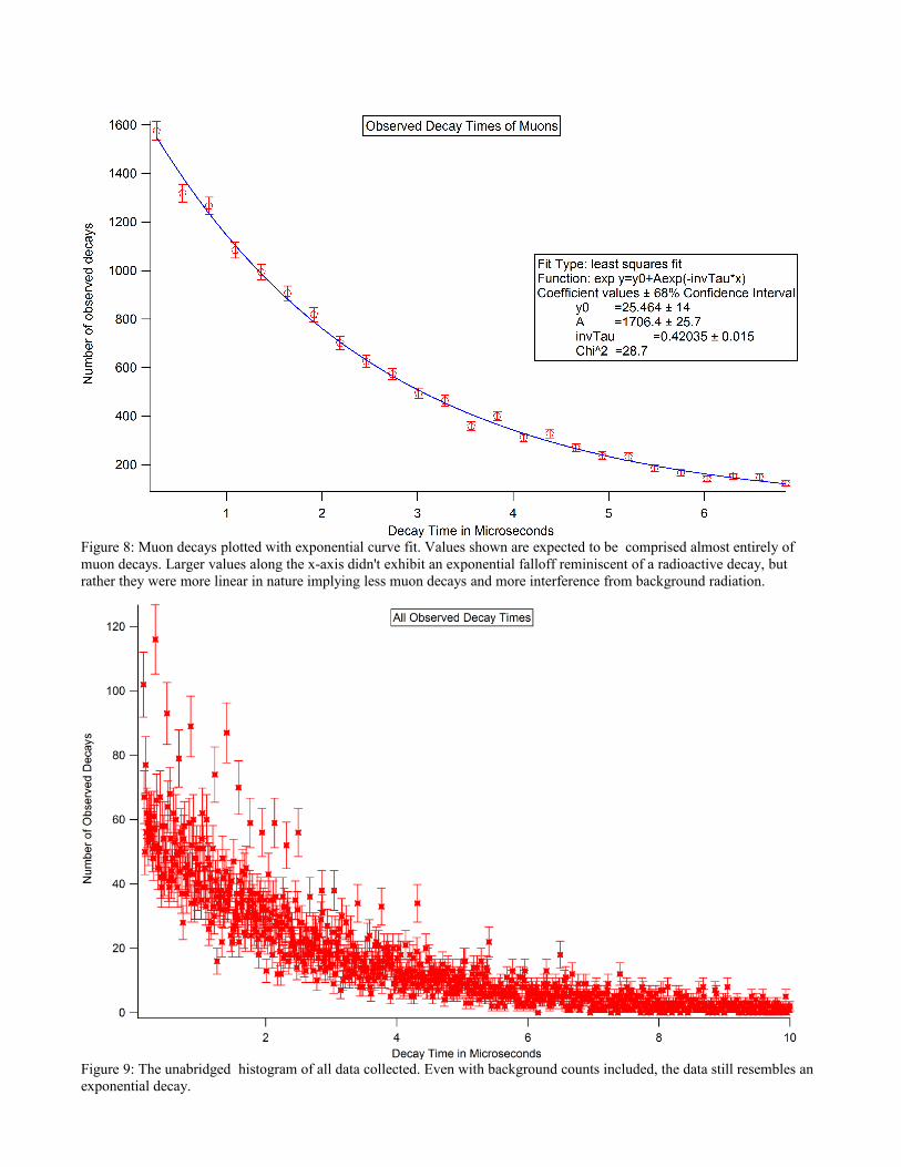
Figure 8: Muon decays plotted with exponential curve fit. Values shown are expected to be comprised almost entirely of muon decays. Larger values along the x-axis didn't exhibit an exponential falloff reminiscent of a radioactive decay, but rather they were more linear in nature implying less muon decays and more interference from background radiation.

Figure 9: The unabridged histogram of all data collected. Even with background counts included, the data still resembles an exponential decay.

Experiment 2: Determination of the Plateau Region of the PMT

Another major factor affecting our measurements was the so called “plateau region” of the PMT. The plateau region is where the number of counts registered are minimally affected by changes in the input voltage. To measure this, we let the Ortec digital counter count the number of incident muons and decays over the same range of voltages from the signal to noise measurements however the time interval was increased to 10 minutes for each voltage increment.

The number of decay counts with respect to voltage is plotted in figure 6. This plot shows the plateau region of 2400 ± 100 volts. We see a median value of 2400 volts which matches exactly the optimum voltage from experiment 1. Thus all further measurements were taken at 2400 volts. As the plateau region spans 100 volts in either direction from our measurement point, and the Ortec power supply we are using to run the PMT has a very low output variation of 0.0025% (or 0.06 volts), it is very unlikely that we would experience a change in voltage that would affect our data in any significant manner.

Experiment 3:Determination of the Conversion Factor from DAQ Digital Units to Seconds

A final factor in our preparation was the fact that the DAQ recorded times not in seconds, but rather in it's own units called “Digital Units” and no conversion factor to seconds was provided.We were, in effect, looking for the solution (m) to

Dm=t (15)

where D is the time measured in DUs, m is the slope of the linear fit, and t is the time expressed in microseconds.

After measuring the output values from the DAQ as described in the introduction, we were able to plot and fit the data using a linear fit shown in figure 7. The slope of the fit line is the conversion factor from DUs to microseconds which was found to be 341.41 ± 1.33 DU/μs. This fit has a reduced 2 value of .81 implying a reasonably good fit to the data.

We are able to tell a few things from this fit, specifically the fact that the conversion factor is essentially constant for all times from 0 to 10 microseconds. In fact, just by looking at the error bars and fit in figure 7, you can see that the only area which exhibits any deviation from the fit is the 9-10 microsecond region which is where we expect to take the least amount of data. This implies that the DAQ is most sensitive and accurate on smaller time scales which is where we expect to see the most muon decays.

Experiment 4: Determination of the Mean Lifetime of a Muon

To actually determine the mean lifetime of the muon, we were required to take a large amount of data for statistical analysis. Our apparatus measured 14984 decay events over the course of approximately five days and measured the time between the incident muon signal and the signal of the decay electron. After removing the first 0.25 microseconds worth of data (as this region is where our instruments were interfering with our measurements) and taking into account the differences in paths and delay times for both the “Start” and “Stop” signals to reach the TAC (127.8 ns and 3.85 ns respectively, which is perhaps our largest source of systematic error, shifting our mean value to a longer lifetime) the data was binned and graphed to create the expected decay curve in figure 8.

Figure 8 is a truncated view of our data while the full curve of all data collected is shown in figure 9. Our data consisted of two main objects 1) an exponential decay of muons primarily at shorter time scales, and 2) a more linear collection

10

of data assumed to be background radiation at longer timescales.

First let us discuss the background radiation. The background radiation was taken to be decay times registered after 9 microseconds as this is approximately 4 times the expected lifetime of a muon, so actual muon decays should be rare after this time. After this data was fitted with a linear fit (with a 2 value of 0.81), a value of the y intercept (or b in y=mx+b) was determined to be approximately 23 counts per bin. This value is low when compared to the number of counts per bin shown in figure 8. In fact, the background radiation doesn't even affect the fit of the exponential data by a significant amount when included. When combined with the fact that the background radiation is essentially constant with respect to time (i.e. it would only shift the y values of the graph by equal amounts and would not affect the actual curvature) we can treat the background as not having an affect on our measurements of a mean lifetime thus we can safely ignore it in our calculations.

The second region of our data (given at shorter timescales) is the decay times of muons. This data was taken to be all values less than 7 microseconds. This data was binned and fitted with an exponential decay curve of the form

y= y0A e- x (16)

where y0 is the background level, A is the number observed at the peak decay time, and is the decay constant. The curve fit gives a value

of1=0.42±0.02 which in turn implies that our

value for the mean decay time of the muon is

=2.38±0.04 s (17)

This curve fit has a reduced 2 value of 1.14 implying that the data closely resembles an exponential decay.

DISCUSSION

The value that we have found for the mean lifetime of the muon (2.38 ± .04 μs) while close to the accepted value (2.19 μs), is approximately two tenths of a microsecond away or about an 8% deviance. This is likely to be caused by one of two factors: 1) some sort of systematic error that we have not accounted for, or 2) a miscalculation in the error of our measurements. One source of error that seems rather likely is when we were testing the signal to noise ratios at various voltages, the original intent was to use an LED pulser to inject signals into our PMT at a constant rate and luminosity. The LED pulser was not available due to time constraints and thus could not be used. Therefore our signal to noise measurements were made from observations of random noise which we were both unable to control and unable to know their true intensity.

The measurement of noise is a large problem for this experiment. If more time had been allotted, we would have made many more measurements of noise and delay times present in our equipment. In addition, the discriminator levels could also be increased by a few 10s of mV in order to block out a large amount of interference and noise while increasing the data collection time to have a greater effect at reducing random error.

We were also measuring decays from both muons and anti-muons with no way to determine which was the source of each decay, although the decay times of these two particles are extremely close, they manner in which they can interact with the scintillator may differ and take a different amount of time requiring a correction for these different interactions. This also implies that our data is comprised of both particles and as we were trying to measure the decay time of a muon only, our data is somewhat inacurate as it includes a large number of decays that are not muons. In order to account for this, the use of an electric

11

field could be employed to direct only negatively charged muons into our scintillator and direct the positive anti-muons away.

CONCLUSION

Overall, in this lab we learned a great deal about how the logic circuits and other NIM electronics worked together to take measurements. The fact that we were not given a prefabricated setup and were forced to decipher the use of each piece of equipment allowed us to gain a deeper understanding of the function of each step in the measurement. Although we were able to measure the mean lifetime of a muon fairly precisely to be 2.38 ± 0.04 μs. The measurement was not as accurate as we had originally hoped, thus leaving room for improvement in the calculation of the errors associated with our apparatus as well as the removal of various forms of noise associated with with the signals that were registering on our equipment.

Acknowledgments

I would like to thank Renae Eaton and Jessica Scheimer for their help in deciphering the complicated electronics of this experiment. They truly kept me from going insane.

12

References:

1) Harris, Randy. Modern Physics (2nd Edition). New York: Addison Wesley, 2007. Pg 18-19. Print.

2) Melissinos, Adrian C. Experiments in modern physics. San Diego: Academic, 2003. Print.

6) Leo, W. R. Techniques for Nuclear and Particle Physics Experiments. 1987. Pg 150-153 Print.

13