Embed Size (px)
Citation preview

SLAC - 320 UC - 34D (E)
MEASUREMENT OF THE B HADRON LIFETIME*
Rene Ashwin Ong
Stanford Linear Accelerator Center
Stanford University
Stanford, California 94305
September 1987
Prepared for the Department of Energy
under contract number DE-AC03-76SF00515
Printed in the United- States of America. Available from the National Techni- cal Information Service, U.S. Department of Commerce, 5285 Port Royal Road, Springfield, Virginia 22161. Price: Printed Copy All, Microfiche AOI.
* Ph.D. Dissertation
Abstract
This thesis presents an experimental determination of the average B hadron
lifetime. B hadrons, particles that contain bottom quarks, are produced from
electron-positron collisions in the PEP storage ring at a center of mass energy c of 29 GeV. Using data taken by the Mark II detector, the decays of B hadrons are
tagged by identifying leptons at high transverse momentum relative to the event
axis. By means of a precision inner drift chamber, the impact parameters of these
lepton tracks are measured with respect to the B hadron production point. From
_ - this impact parameter distribution, the average B hadron lifetime is then deduced.
Based on a sample of 617 leptons, this lifetime is found to be:
7b = (0.98 * 0.12 AZ 0.13) X lo-l2 set ,
where the first error is statistical and the second systematic.
It is believed that the B hadron lifetime is largely determined by the lifetime of
the bottom quark. This thesis therefore presents a measurement of a fundamental
property of bottom quark decay via the weak interaction. In addition, in
conjunction with other experimental results, this measurement can be used to place
constraints on models of quark mixing.
ii
Acknowledgments
This thesis builds upon the careful and detailed work of a great many people.
First and foremost, I wish to thank all the members, past and present, of the Mark II
collaboration. With pleasure, I acknowledge the guidance and motivation provided
by my advisor John Jaros, and the help and warm friendship offered to me by my
office-mate Ken Hayes. These gentlemen were always available for long discussions
and keen insight concerning my work. I also thank Lydia Beers for much assistance
and joie de oiure over the years.
The measurement presented in this thesis uses many of the ideas (and even
some of the bug-free computer code) of physicists who have done similar analyses
on the Mark II experiment, namely Nigel Lockyer, Larry Gladney, Dan Amidei, and
Mark Nelson. I received invaluable day-to-day help from my comrades Ray Cowan,
Keith Riles, Dean Karlen, and Bruce LeClaire, and numerous useful suggestions
from George Trilling and Vera Lfith. I also acknowledge the members of my Ph.D.
committee, the staff and faculty of the Stanford Physics department, and all the
people who helped proofread the thesis.
I first became interested in science from discussions with my father. After
discovering I was too messy for chemistry, I turned to particle physics thanks to the
motivating influences of Dan Sinclair, Howard Gordon, and Larry Sulak. I ended
up at Stanford largely because of the encouragement of Martin Perl, who has been
especially supportive of me over the years.
Graduate school was a wonderful experience, in no small part because of the
friends that I have made. I will miss Chris Wendt and Alex Harwit, roommates
that have put up with me. I will also fondly remember time spent with Natalie
Roe, tennis matches with Fred Bird, and dinners with Patricia Stuart. My good
pals Robert Johnson and Steve Wagner have helped me to enjoy myself, and the
love of Anna Green has brightened up my life. Most of all, however, it was the
strong and enduring friendship of Harry Nelson, and the love from my parents and
sister, that helped me to complete this endeavour.
. . . 111
Table of Contents
Abstract . . . . . . . . .
Acknowledgments . . . . . . .
c Table of Contents . . . . . . . .
List of Tables . . . . . . . . .
List of Figures . . . . . . . .
1. Introduction . . . . . . . .
1.1 The Standard Model . . . . . . - 1.2 B Hadron Production . . . . .
1.2.1 Quark production in e+e- annihilations
1.2.2 Quark fragmentation . . . .
1.3 B Hadron Decay . . . . . .
.
.
.
.
.
.
.
.
.
.
.
1.3.1 Quark decay and the Kobayashi-Maskawa matrix
1.3.2 Heavy quark decay . . . . . .
1.3.3 Bottom quark decay . . . . .
1.3.4 Improvements to the spectator decay model
1.3.5 Beyond the spectator decay model
1.3.6 Summary of B decay rate calculations
1.4 Testing the KM Model . . .
1.5 Analysis Objective . . . .
1.6 Thesis Outline . . . .
2. Experimental Apparatus . . .
2.1 The PEP Storage Ring . . .
2.2 The Mark II Detector: Overview .
2.3 Beam Position Monitors - . .
2.4 Beam Pipe and Detector Materials
2.5 Vertex Chamber . . . .
2.6 Main Drift Chamber . . .
2.7 Magnet Coil . . . . .
2.8 Liquid Argon Calorimeter . .
2.9 Muon System . . . . l
.
.
.
.
.
.
.
.
.
.
.
.
.
.
.
.
.
.
.
.
.
.
.
.
.
.
.
.
.
.
.
.
.
.
.
.
.
.
.
.
.
.
.
.
.
.
.
.
.
.
.
.
.
.
.
.
.
.
.
.
.
.
.
.
.
.
.
.
.
.
.
.
.
.
.
.
.
.
.
.
.
.
.
.
.
.
.
.
.
.
.
.
.
.
.
.
.
.
.
.
.
.
.
.
.
.
.
.
.
.
.
.
.
.
.
.
.
.
.
.
.
.
.
.
.
.
.
.
.
.
.
.
.
.
.
.
.
.
.
.
.
.
.
.
.
.
.
.
.
.
.
.
.
.
.
.
.
.
.
.
l
ii . . . 111
iv
ix
xi
1 2 5 5 6
10 10 12 13 14 17 19 20 23 26 27 27 27 30 30 31 35 37 38 39
iv
c
2.10 Other Systems . . . .
2.10.1 Time of flight system . .
2.10.2 Endcap calorimeters . .
2.10.3 Small angle tagging system .
2.11 Event Trigger System . . .
2.12 Operating Conditions . . .
2.12.1 Drift Chamber operation .
2.12.2 Vertex Chamber operation .
2.12.3 Test chamber study . .
3. Event Reconstruction and Simulation
3.1 Charged Track Reconstruction .
3.2 Monte Carlo Simulation . .
3.3 Optimization of the Monte Carlo
3.3.1 Charged particle multiplicity
3.3.2 Event thrust . . . .
.
.
.
.
.
.
.
.
.
.
.
.
.
.
.
.
.
.
.
.
.
.
.
.
.
.
.
.
.
.
.
.
.
.
.
.
.
.
.
.
.
.
.
.
.
.
.
.
.
.
.
.
.
.
.
.
.
.
.
*
.
.
.
.
.
.
.
.
.
.
.
.
.
.
l
.
.
.
.
.
.
.
.
.
.
.
.
.
.
.
3.3.3 Charm and bottom hadron production and branching ratios
T
-_ ** -- I
3.3.4 Charm and bottom hadron decay spectra . .
3.3.5 Charm and bottom hadron lifetimes . . .
4. Tracking and Resolution Studies . . . . .
4.1 Vertex Chamber Tracking . . . . . .
4.2 Wire Residual Survey . . . . . . .
4.3 Study of Isolated Tracks . . . . . .
4.3.1 Isolated track x2 . . . . . . .
4.3.2 Bhabha separation distance . . . . .
4.3.3 Measurement of multiple scattering contribution
. : 4.4 Beam Parameters . . . . . . . .
4.4.1 Beam position determination . . . .
4.4.2 Beam size determination . . . . .
4.5 Study of Tracks in Hadronic Events . . . .
4.5.1 Hadronic track x2 . . . . . . .
4.5.2 The time-slewing effect . . . . . .
4.5.3 Probable cause of the time-slewing effect . .
.
.
.
.
.
.
.
.
.
.
.
.
.
.
.
.
. 41
. 41
. 42
. 42
. 42
. 43
. 43
. 44
. 45
. 49
. 50
. 51
. 53
. 53
. 53
. 55
. 58
. 60
. 63
. 63
. 64
. 67
. 67
. 67
. 69
. 72
. 72
. 72
. 75
. 75
. 77
. 80
V
4.5.4 The fix to the time-slewing effect . . .
4.6 Track Quality Cuts . . . . . .
5. Lepton Identification . . . . . . .
5.1 Electron Identification . . . . . .
5.1.1 Identification algorithm . . . . . c 5.1.2 Identification efficiency . . . . .
5.1.3 Hadron mis-identification . . . .
5.1.4 Electrons from conversions and Dalitz decays
5.2 Muon Identification . . . . . . . - 5.2.1 Identification algorithm . . . . .
5.2.2 Identification efficiency . . . . .
5.2.3 Hadron punchthrough . . . . .
5.2.4 Muons from decays . . . . . .
6. Inclusive Lepton Analysis . . . . . .
6.1 Hadronic Event Selection . . . . .
6.2 Lepton Selection . . . . . . .
6.3 Prompt Lepton Signal . . . . . .
6.3.1 Raw signal . . . . . . .
6.3.2 Expected background to the electron signal
6.3.3 Expected background to the muon signal .
6.4 Description of the Lepton (p,pt) Fit . . .
.
.
.
.
.
.
.
.
.
.
.
.
.
.
.
.
.
.
.
.
.
6.4.1 Parameterization for the number of predicted leptons
6.4.2 The variables used in the parameterization .
6.4.3 The Monte Carlo (p,pt) probability distributions
6.4.4 The full fit . . . . . . . .
6.5 Inclusive Lepton Results and Discussion . . .
6.5.1 Systematic errors . . . . . . .
6.5.2 Checks on the fit . . . . . . .
6.5.3 Composition of the predicted signal . . .
6.5.4 Selecting B and C enhanced regions . . .
6.5.5 Comparison with other experiments . . .
7. The Impact Parameter Method . . . . . .
vi
.
.
.
.
.
.
.
.
.
.
.
.
.
.
.
.
.
.
.
.
.
.
.
.
.
.
.
.
.
.
.
.
.
.
.
.
.
.
.
.
.
.
.
.
.
.
.
.
.
.
.
.
.
. 80
. 82
. 85
. 86
. 86
. 88
. 89
. 90
. 92
. 92
. 93
. 94
. 97
. 99
. 100
. 101
. 102
. 102
. 102
. 104
. 106
. 106
. 107
. 108
. 110
. 111
. 111
. 114
. 114
. 116
. 119
. 121
7.1 Impact Parameter Definition . . . . . .
7.2 Resolution Effects on the Impact Parameter Distribution
7.3 Lepton Impact Parameter Distributions . . .
7.4 Determining the B Production Point . . . .
7.4.1 Introduction on the use of the decay length method c 7.4.2 The algorithm to find the B production point
7.4.3 Checks on the production point algorithm .
7.5 Application of the Production Point Algorithm
7.6 Summary of Cuts Applied to the Lepton Sample _. - 8. The Lifetime Fits . . . . . . . .
8.1 The Fitting Function . . . . . .
8.2 Inputs to the Fitting Function . . . .
8.2.1 The lepton fractions . . . . .
8.2.2 The background contribution . . .
8.2.3 The prompt lepton contribution . . .
8.2.4 The physics functions . . . . .
8.2.5 The resolution function . . . . .
8.3 Fitting the Impact Parameter Distributions .
8.4 Results of the Fits . . . . . . .
9. Checks and Systematic Errors . . . . .
9.1 Checks on the Analysis and Fitting Procedures
9.1.1 Average charm lifetime . . . . .
9.1.2 Two-photon cuts . . . . . . v 9.1.3 Tau lifetime determination . . . .
9.1.4 Consistency checks . . . . . .
9.1.5 Simple mean determination of the lifetimes
9.1.6 Measuring rb in the Monte Carlo . . .
9.1.7 Checking the statistical errors . . .
9.2 Systematic Errors . . . . . . .
9.2.1 Uncertainty in the lepton fractions . .
9.2.2 Fragmentation uncertainty . . . .
92.3 Uncertainty in the resolution . . .
.
.
.
.
.
.
.
.
.
.
.
.
.
.
.
.
.
.
.
.
.
.
.
.
.
.
.
.
.
.
.
.
.
.
.
.
.
.
.
.
.
.
.
.
.
l
.
.
.
.
.
.
.
.
.
.
.
.
.
.
.
.
.
.
.
.
.
.
.
.
.
.
.
.
.
.
.
.
.
.
.
.
.
.
.
.
.
.
. 121
. 123
. 126
. 127
. 129
. 130
. 133
. 135
. 137
. 141
. 141
. 142
. 142
. 143
. 145
. 148
. 150
. 155
. 156
. 160
. 160
. 160
. 160
. 161
. 164
. 165
. 167
. 168
. 169
. 170
. 171
. 173
vii
9.2.4 Measurement bias and analysis cuts
9.2.5 Thrust uncertainties . . .
c
9.2.6 Fitting procedure assumptions .
9.2.7 Two-photon background . .
9.2.8 Non-charm decays of bottom .
9.29 Other systematic errors . . .
9.2.10 Summary of the systematic errors
IO. Conclusions . . . . . . .
10.1 Summary of Lifetime Results . . . - IO.2 Inclusive Lepton Results . . .
10.3 Other Results . . . . .
IO.4 B Lifetimes From Around the World
10.5 Constraints on the Standard Model .
Appendix A. Event Backgrounds . . .
A.1 Two-Photon Hadron Production .
.
.
.
.
.
.
.
.
.
.
.
.
.
.
.
A.1.1 Cuts to remove two-photon background
A.1.2 Two-photon Monte Carlo study . .
A.2 Tau Pair Production . . . . .
Appendix B. The Decay Length Method . .
B.1 The Decay Length Formulae . . .
B.2 Uncertainty in the Particle Direction . .
Appendix C. The Longest Lived Event . . .
REFERENCES . . . . . . . . .,
_ _. . i - - .:
-
.
.
.
.
.
.
.
.
.
.
.
.
.
.
.
.
.
.
.
.
.
.
.
.
.
.
.
.
.
.
.
.
.
.
.
.
.
.
.
.
.
.
.
.
.
.
.
.
.
.
.
.
.
.
.
.
.
.
.
.
.
.
.
.
.
.
.
.
.
.
.
.
.
.
.
.
.
.
.
.
.
.
.
.
.
.
.
.
.
.
.
.
. 175
. 176
. 178
. 178
. 178
. 178
. 179
. 181
. 181
. 182
. 183
. 183
. 185
. 189
. 189
. 189
. 191
. 194
. 197
. 197
. 202
. 205
. 209
. . . Vlll
1.1 1.2
d 1.3 2.1 2.2 2.3 3.1
_ - 3.2 3.3 3.4 4.1 4.2 5.1 5.2 5.3 5.4 5.5 5.6 5.7 6.1 6.2 6.3 6.4
_* -- 6.5 : - .:. 6.6 6.7 6.8 6.9
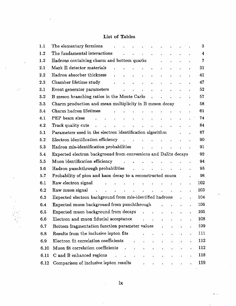
List of Tables
The elementary fermions . . . . . . . .
The fundamental interactions . . . . . . .
Hadrons containing charm and bottom quarks . . .
Mark II detector materials . . . . . . . . Hadron absorber thickness . . . . . . . .
Chamber lifetime study . . . . . . . . Event generator parameters . . . . . . . B meson branching ratios in the Monte Carlo . . . .
Charm production and mean multiplicity in B meson decay Charm hadron lifetimes . . . . . . . . PEP beam sizes . . . . . . . . . .
Track quality cuts . . . . . . . . . . Parameters used in the electron identification algorithm .
Electron identification efficiency . . . . . . .
Hadron mis-identification probabilities . . . . .
Expected electron background from conversions and Dalitz decays
Muon identification efficiency . . . . . . Hadron punchthrough probabilities . . . . . Probability of pion and kaon decay to a reconstructed muon
Raw electron signal . . . . . . . .
Raw muon signal . . . . . . . . . Expected electron background from mis-identified hadrons
Expected muon background from punchthrough . .
Expected muon background from decays . . . .
Electron and muon fiducial acceptance . . . .
Bottom fragmentation function parameter values . .
Results from the inclusive lepton fits . . . .
Electron fit correlation coefficients . . . . .
6.10 Muon fit correlation coefficients . . . . . .
6.11 C and B enhanced regions . . . . . . .
6.12 Comparison of inclusive lepton results . . . .
.
.
.
.
l
.
.
.
.
.
.
.
.
.
.
.
.
.
.
.
.
.
.
.
.
.
.
.
.
.
.
.
.
.
.
.
.
.
.
.
.
.
.
.
3 4 7
31 41 47 52 57 58 61 74 84 87 90 91 92 94 95 98
102 103 104 L 105 105 108 io9 111 112 112 118 119
ix
7.1 7.2 8.1
8.2 8.3
.L 8.4 9.1 9.2 9.3 9.4 -. - 9.5 9.6 9.7 9.8 10.1 10.2 A.1 A.2 A.3 A.4 c.1
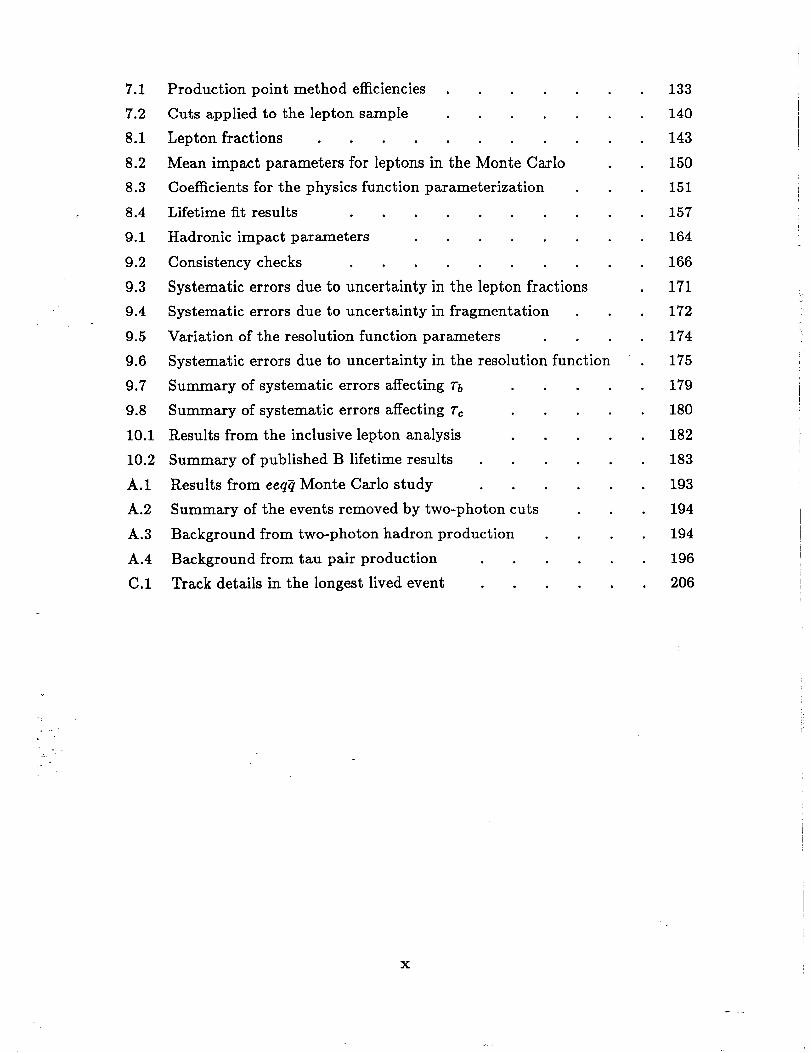
Production point method efficiencies . . . . . Cuts applied to the lepton sample . . . . . Lepton fractions . . . . . . . . . Mean impact parameters for leptons in the Monte Carlo Coefficients for the physics function parameterization .
Lifetime fit results . . . . . . . . Hadronic impact parameters . . . . . .
Consistency checks . . . . . . . . Systematic errors due to uncertainty in the lepton fractions Systematic errors due to uncertainty in fragmentation .
Variation of the resolution function parameters . .
.
.
.
.
.
.
.
.
.
.
Systematic errors due to uncertainty in the resolution function Summary of systematic errors affecting 7b . . . .
Summary of systematic errors affecting & . . . .
Results from the inclusive lepton analysis . . . .
Summary of published B lifetime results . . . . .
Results from eeqg Monte Carlo study . . . . . Summary of the events removed by two-photon cuts . .
Background from two-photon hadron production . . . Background from tau pair production . . . . .
Track details in the longest lived event . . . . .
. 133
. 140
. 143
. 150
. 151
. 157
. 164
. 166
. 171
. 172
. 174
. 175
. 179
. 180
. 182
. 183
. 193
. 194
. 194
. 196
. 206
X
1.1 1.2 1.3 I 1.4 1.5 1.6 1.7
. 1.8 2.1 2.2 2.3 2.4 2.5 2.6 2.7 2.8 2.9 2.10 2.11 2.12 2.13 2.14 2.15
_* _- 2.16 i . .;. 2.17
3.1 3.2 3.3 3.4 3.5 3.6
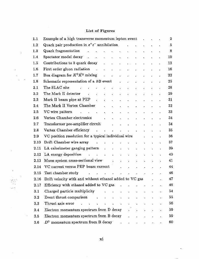
List of Figures
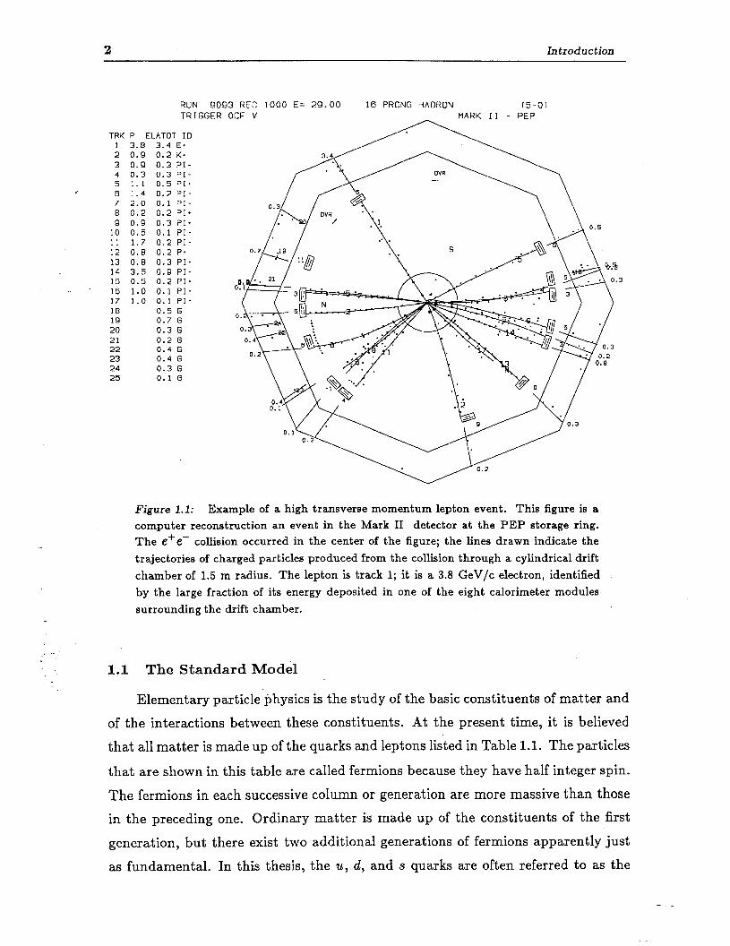
Example of a high transverse momentum lepton event
Quark pair production in e+e- annihilation .
.
.
.
.
.
.
.
.
.
.
.
.
.
.
.
.
.
.
.
.
.
.
.
.
l
.
.
.
.
.
.
.
.
.
.
Quark fragmentation . . . . Spectator model decay . . . .
Contributions to b quark decay . .
First order gluon radiation . . .
Box diagram for K*@ mixing . .
Schematic representation of a BB event
The SLAC site . . . . .
The Mark II detector . . . . Mark II beam pipe at PEP . . .
The Mark II Vertex Chamber . .
VC wire pattern . . . . . Vertex Chamber electronics . .
Transformer pre-amplifier circuit .
Vertex Chamber efficiency . . .
.
.
.
.
.
.
.
l
.
.
.
.
.
.
VC position resolution for a typical individual wire Drift Chamber wire array . . . . . LA calorimeter ganging pattern . . . .
LA energy deposition . . . . . .
Muon system cross-sectional view . . .
VC current versus PEP beam current . .
Test chamber study . . . . . .
.
.
.
.
.
.
.
.
.
.
.
.
.
.
.
.
.
.
.
.
.
.
.
Drift velocity with and without ethanol added to VC gas Efficiency with ethanol added to VC gas . . . .
Charged particle multiplicity . . . . . . Event thrust comparison . . . . . . .
Thrust axis error . . . . . . . . .
Electron momentum spectrum from D decay . ’ . .
Electron momentum spectrum from B decay . . .
Do momentum spectrum from B decay . . . .
. . 2
. . 5
. . 8
. . 10
. . 13
. . 16
. . 22
. . 25
. . 28
. . 29
. . 31
. . 32
. . 33
. . 34
. . 34
. . 35
. . 36
. . 37
. . 39
. . 40
. . 41
. . 44
. . 46
. . 47
. . 48
. . 54
. . 55
. . 56
. . 59
. . 59
. . 60
xi
4.1 4.2 4.3 4.4 4.5 4.6 4.7 4.8 4.9 4.10 4.11 4.12 4.13 4.14 5.1 5.2 6.1 6.2 6.3 6.4 6.5 7.1 7.2 7.3 7.4 7.5 7.6 7.7 7.8 7.9 7.10
7.11 7.12 7.13
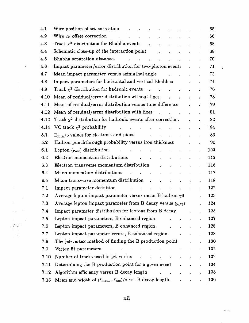
Wire position offset correction . . . . . . Wire TO offset correction . . . . . . . Track ~2 distribution for Bhabha events . . . . Schematic close-up of the interaction point . . .
Bhabha separation distance. . . . . . . Impact parameter/error distribution for two-photon events
Mean impact parameter versus azimuthal angle . .
Impact parameters for horizontal and vertical Bhabhas Track ~2 distribution for hadronic events . . . .
Mean of residual/error distribution without fixes. . .
Mean of residual/error distribution versus time difference
Mean of residual/error distribution with fixes . . .
Track ~2 distribution for hadronic events after correction.
VC track ~2 probability . . . . . . . Emin/p values for electrons and pions l . . .
Hadron punchthrough probability versus iron thickness Lepton (p,pt) distribution . . . . . . . Electron momentum distributions . . . . .
Electron transverse momentum distribution . . . Muon momentum distributions . . . . . .
Muon transverse momentum distribution . . . . Impact parameter definition . . . . . .
Average lepton impact parameter versus mean B hadron 7~
Average lepton impact parameter from B decay versus (p,pt) Impact parameter distribution for leptons from B decay
Lepton impact parameters, B enhanced region . . Lepton impact parameters, B enhanced region . .
Lepton impact parameter-errors, B enhanced region .
The jet-vertex method of finding the B production point Vertex fit parameters . . . . . . . .
Number of tracks used in jet vertex . . . . .
Determining the B production point for a given event .
Algorithm efficiency versus B decay length . . .
Mean and width of (Smeas-6mc)/a VS. B decay length. .
.
.
.
.
.
.
.
.
.
.
.
.
.
.
.
.
.
.
.
.
.
.
.
.
.
.
.
.
.
.
.
.
. 65
. 66
. 68
. 69
. 70
. 71
. 73
. 74
. 76
. 78
. 79
. 81 * 82 . 84 . 89 . 96 . 103 . 115 . 116 . 117 . 118 . 122 . 123 . 124 . 125 . 127 . 128 . 128 . 130 . 132 . 132 . 134
. 135
. 136
xii
7.14 7.15
7.16 7.17
8.1 c 8.2
8.3 8.4 8.5 8.6 8.7 8.8 8.9 8.10 8.11 8.12 9.1 9.2 9.3 9.4
9.5
9.6 9.7
9.8
9.9 9.10
. _. - : 9.11 - - -;
_- : 10.1 10.2 10.3 A.1
A.2 A.3 B.1
Checking the production point algorithm in the data . Jet-jet ~2 using the production point algorithm. . .
Lepton impact parameters, B enhanced region . . Lepton impact parameter errors, B enhanced region .
Impact parameter distribution for hadronic tracks . . Normalized hadronic track impact parameter distribution
Exact impact parameter distribution . . . .
Physics function for leptons from B decay . . .
Physics function for leptons from B decay . . .
Definition of the fract variable . . . . . . Fract distribution for hadronic tracks . . . .
Impact parameter/error for low fract hadronic tracks .
Two dimensional log likelihood contours . . . . Log likelihood contour as a function of ~b . . .
.
.
.
.
.
.
.
.
.
.
.
.
.
.
Fit to lepton impact parameter distribution, B enhanced region
Fit to lepton impact parameter distribution, C enhanced region
Electron impact parameters, events removed by two-photon cuts
Impact parameters for tracks in tau events . . .
Determination of the tau lifetime . . . . .
Lepton impact parameters, high fract . . . .
Electron and muon impact parameter distributions .
Simple mean calculation . . . . . . . Measuring the B lifetime in the Monte Carlo . . .
Effect of the B fraction on the measured lifetime . .
Effect of <ZQ on the measured B lifetime . . .
Uncertainty in the resolution function . . . .
The effect of truncating the impact parameter distribution
B lifetimes from around the world . . . . .
World average B-lifetime as a function of time . .
Constraints on the KM terms for B decay . . .
A two-photon event in the data . . . . . .
Diagrams for two-photon hadron production . . .
Diagrams for tau pair production . . . . .
Measurement of the tau decay length . . . .
.
.
.
.
.
.
.
.
.
.
.
.
.
.
.
.
.
.
.
.
.
.
.
.
.
.
.
.
.
.
.
.
.
.
.
.
.
.
.
.
.
.
.
.
.
.
.
.
.
.
137 138
138 139 145 146 147 149 151
152 153 154
156 158 159 159 161 162 163 165 166 168 169 172 173 174 177 184 185 186 190
192
195 198

B.2 The effect of including thrust uncertainties . . . . . 203 C.1 An interesting event . . . . . . . . . . 206 C.2 Enlarged view of the event . . . . . . . . . 207
xiv
Chapter I
Introduction
This thesis presents an experimental determination of the lifetime of hadrons
containing bottom quarks (B hadrons). B hadrons are produced from electron-
positron collisions in the PEP storage ring at a center of mass energy of 29 GeV.
These hadrons travel a short distance (typically 6OOpm) and decay via the weak
interaction into a number of particles. The decay particles are then observed in the
Mark II detector which surrounds the interaction point. Approximately 25 % of B
hadrons decay to leptons (an electron, muon, or tau). Because of the heavy bottom
quark mass, these leptons often carry a large amount of momentum perpendicular
to the original quark direction. This transverse component of momentum (pt) is
used to separate B hadron decays from the decays of lighter hadrons. Figure 1.1,
shows a high pt lepton event observed in the Mark II detector.
.
: - .:
Since the lepton track is reliably known to have come from B hadron decay, its
trajectory contains information about the parent lifetime. In this thesis, we measure
the distance of closest approach between the lepton track and the point where the
B is produced. The B hadron lifetime is then determined from the distribution of
such distances for a sample of 617 lepton tracks.
The remainder of this chapter provides a brief summary of the relevant
theoretical considerations associated with the measurement. The Standard Model
of electro-weak interactions is introduced, followed by a description of heavy quark
production and decay. The possible constraints on Standard Model parameters
from the B lifetime measurement are discussed. At the end of the chapter, the
analysis objectives and an outline of the thesis are presented.
2 Introduction
RUN 9093 REC 1000 E= 29.00 16 PRONG HADRON (5-0) TRIGGER OCF V MARK II - PEP
TRK P ELATOT IO 1 3.8 3.4 E+ 2 0.9 0.2 K+ 3 0.9 0.3 PI- 4 0.3 0.3 PI- 5 1.1 0.5 PI+ 6 1.4 0.2 PI- 7 2.0 0.1 PI- 8 0.2 0.2 PI+ 9 0.9 0.3 PI+
10 0.5 0.1 PI- 11 1.7 0.2 PI- 12 0.8 0.2 P+ 13 0.8 0.3 PI* 14 3.5 0.9 PI- 15 0.5 0.2 PI+ 16 1.0 0.1 PI+ 17 1.0 0.1 PI- 18 0.5 G 19 0.7 G 20 0.3 G 21 0.2 G 22 0.4 G 23 0.4 G 24 0.3 G 25 0.1 G
Figure 1.1: Example of a high transverse momentum lepton event. This figure is a computer reconstruction an event in the Mark II detector at the PEP storage ring. The e’e- collision occurred in the center of the figure; the lines drawn indicate the trajectories of charged particles produced from the collision through a cylindrical drift chamber of 1.5 m radius. The lepton is track 1; it is a 3.8 GeV/c electron, identified by the large fraction of its energy deposited in one of the eight calorimeter modules surrounding the drift chamber.
1.1 The Standard Model
Elementary particle physics is the study of the basic constituents of matter and
of the interactions between these constituents. At the present time, it is believed
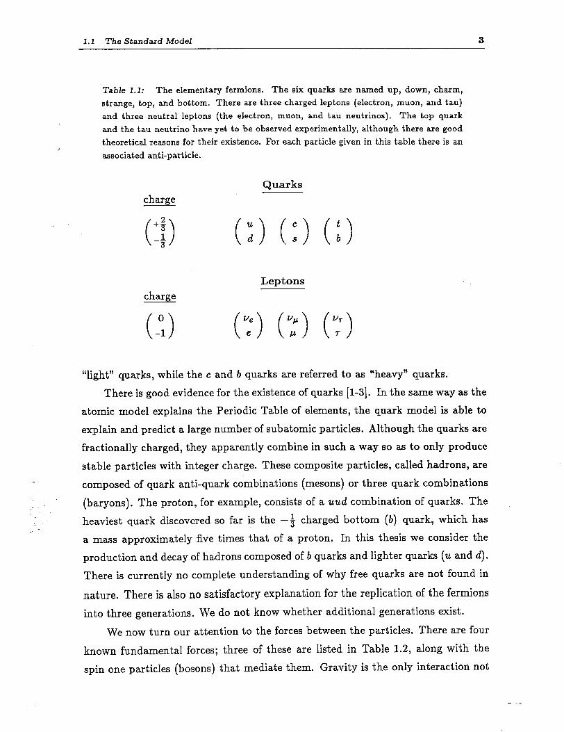
that all matter is made up of the quarks and leptons listed in Table 1.1. The particles
that are shown in this table are called fermions because they have half integer spin.
The fermions in each successive column or generation are more massive than those
in the preceding one. Ordinary matter is made up of the constituents of the first
generation, but there exist two additional generations of fermions apparently just
as fundamental. In this thesis, the U, d, and s quarks are often referred to as the
1.1 The Standard Model 3
Table 1.1: The elementary fermions. The six quarks are named up, down, charm, strange, top, and bottom. There are three charged leptons (electron, muon, and tau) and three neutral leptons (the electron, muon, and tau neutrinos). The top quark and the tau neutrino have yet to be observed experimentally, although there are good theoretical reasons for their existence. For each particle given in this table there is an associated anti-particle.
Quarks charge
+- : ( > -- i Leptons
charge
“light” quarks, while the c and b quarks are referred to as “heavy” quarks.
There is good evidence for the existence of quarks [l-3]. In the same way as the
atomic model explains the Periodic Table of elements, the quark model is able to
explain and predict a large number of subatomic particles. Although the quarks are
fractionally charged, they apparently combine in such a way so as to only produce
stable particles with integer charge. These composite particles, called hadrons, are
composed of quark anti-quark combinations (mesons) or three quark combinations
(baryons). The proton, for example, consists of a uud combination of quarks. The
heaviest quark discovered so far is the -8 charged bottom (b) quark, which has
a mass approximately five times that of a proton. In this thesis we consider the
production and decay of hadrons composed of b quarks and lighter quarks (2~ and d).
There is currently no complete understanding of why free quarks are not found in
nature. There is also no satisfactory explanation for the replication of the fermions into three generations. We do not know whether additional generations exist.
We now turn our attention to the forces between the particles. There are four
known fundamental forces; three of these are listed in Table 1.2, along with the
spin one particles (bosons) that mediate them. Gravity is the only interaction not
4 Introduction
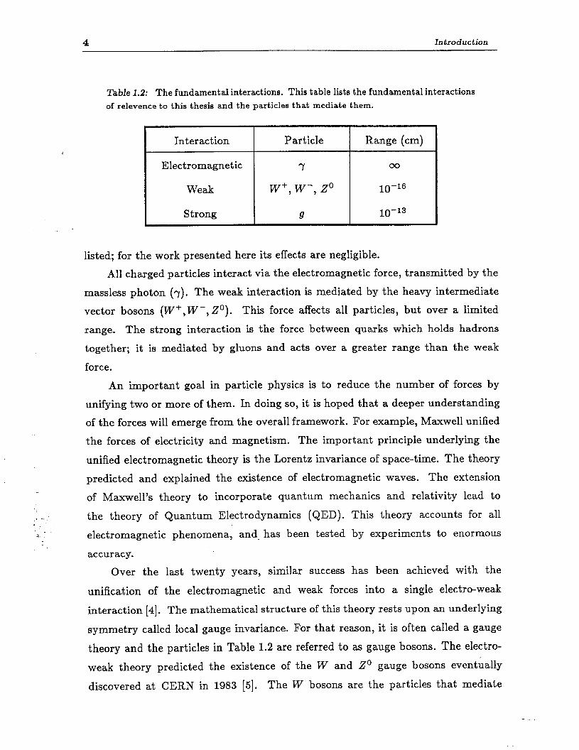
Table 1.2: The fundamental interactions. This table lists the fundamental interactions of relevence to this thesis and the particles that mediate them.
Interaction Particle Range (cm)
Electromagnetic 7 00
Weak w+, w-, 2-O IO--l6
Strong g lo-l3
listed; for the work presented here its effects are negligible.
All charged particles interact via the electromagnetic force, transmitted by the
massless photon (7). The weak interaction is mediated by the heavy intermediate
vector bosons (W’, W-, 2’). This force affects all particles, but over a limited
range. The strong interaction is the force between quarks which holds hadrons
together; it is mediated by gluons and acts over a greater range than the weak
force.
_ _. - i - -;
An important goal in particle physics is to reduce the number of forces by
unifying two or more of them. In doing so, it is hoped that a deeper understanding
of the forces will emerge from the overall framework. For example, Maxwell unified
the forces of electricity and magnetism. The important principle underlying the
unified electromagnetic theory is the Lorentz invariance of space-time. The theory
predicted and explained the existence of electromagnetic waves. The extension
of Maxwell’s theory to incorporate quantum mechanics and relativity lead to
the theory of Quantum Electrodynamics (QED). This theory accounts for all
electromagnetic phenomena, and- has been tested by experiments to enormous
accuracy.
Over the last twenty years, similar success has been achieved with the
unification of the electromagnetic and weak forces into a single electro-weak
interaction [4]. The mathematical structure of this theory rests upon an underlying
symmetry called local gauge invariance. For that reason, it is often called a gauge
theory and the particles in Table 1.2 are referred to as gauge bosons. The electro-
weak theory predicted the existence of the VV and 2’ gauge bosons ever&ally
discovered at CERN in 1983 [5]. The VV b osons are the particles that mediate
1.2 B Hadron Production 5
quark decay.
Similarly, the concept of local gauge invariance has been applied to the force
between quarks, the strong interaction. This application has yielded the gauge
theory of Quantum Chromodynamics (&CD) based on the symmetry properties of < a quantity known as color. The color force is mediated by gluons, whose existence
is supported by the observation of three jet events in e+e- annihilation [6].
The Standard Model of particle physics incorporates the electro-weak theory,
&CD, and the particles listed in Table 1.1 and Table 1.2.* This model contains a
- number of parameters that are not fixed by the model but which must come from
experiments.t We will see later that, by using the results presented in this thesis,
we can put constraints on two of these parameters.
1.2 B Hadron Production
1.2.1 Quark production in e+e- annihilations
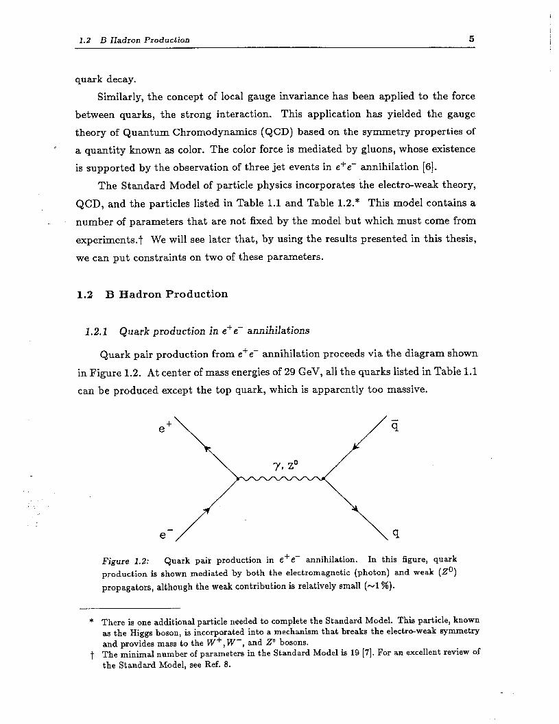
Quark pair production from e+e- annihilation proceeds via the diagram shown
in Figure 1.2. At center of mass energies of 29 GeV, all the quarks listed in Table 1.1
can be produced except the top quark, which is apparently too massive.
Figure 1.2: Quark pair production in e+e- annihilation. In this figure, quark production is shown mediated by both the electromagnetic (photon) and weak (Z”) propagators, although the weak contribution is relatively small (~1%).
* There is one additional particle needed to complete the Standard Model. This particle, known as the Higgs boson, is incorporated into a mechanism that breaks the electro-weak symmetry and provides mass to the W’, IV-, and 2” bosons.
i The minimal number of parameters in the Standard Model is 19 [7]. For an excellent review of the Standard Model, see Ref. 8.
6 In trod uc tion
The cross section for fermion pair production from single-photon annihilation
can be calculated from QED:
a(e+e-+f+f-) = C41irq2 , cm
(1 1) .
where Q! is the QED coupling constant (- l/137), Ecm is the center of mass energy,
and q is the fermion charge. C is a color factor, which for the production of lepton
pairs (e.g. p+p- ) is equal to 1, while for the production of quark pairs (e.g. & )
_ is equal to 3. In Eqn. 1.1, phase space effects, QED loop corrections, and QCD
corrections to the cross section are ignored.
From Eqn. 1.1, we see that quarks are produced in e+e- annihilation in
proportion to their charge squared. Therefore, c quark production should comprise
4/ll and b quark production l/11 of the total quark production. The produced
quarks do not appear as free particles in the final state; they combine with other
quarks in a process called fragmentation. The principal hadrons containing heavy
quarks are given in Table 1.3 . The relative production of these various hadrons is
discussed in Chapter 3.
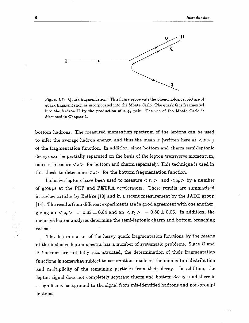
1.2.2 Quark fragmentation
The fragmentation process describes the transformation of quarks into
observable final state hadrons. This process cannot be calculated by perturbative
QCD and is only phenomenologically understood. This phenomenology is illustrated
in Figure 1.3. A bare outgoing quark is turned into a hadron by the production of
a qij pair and the subsequent “dressing” of the bare quark by the anti-quark half of _* -- _ .:
the pair. The quark half of the q?j pair is free to carry on the fragmentation process.
This process continues until there -is insufficient energy to produce new qij pairs.
It is customary to parameterize fragmentation by a probability function (or
fragmentation function), f(z), where x is defined as the fraction of energy and
momentum parallel to the quark direction carried away by the hadron:
Note that in this definition, the energy and momentum used in the denominator
are not equal to the beam energy because of gluon and initial state radiation.
1.2 B Hadron Production 7
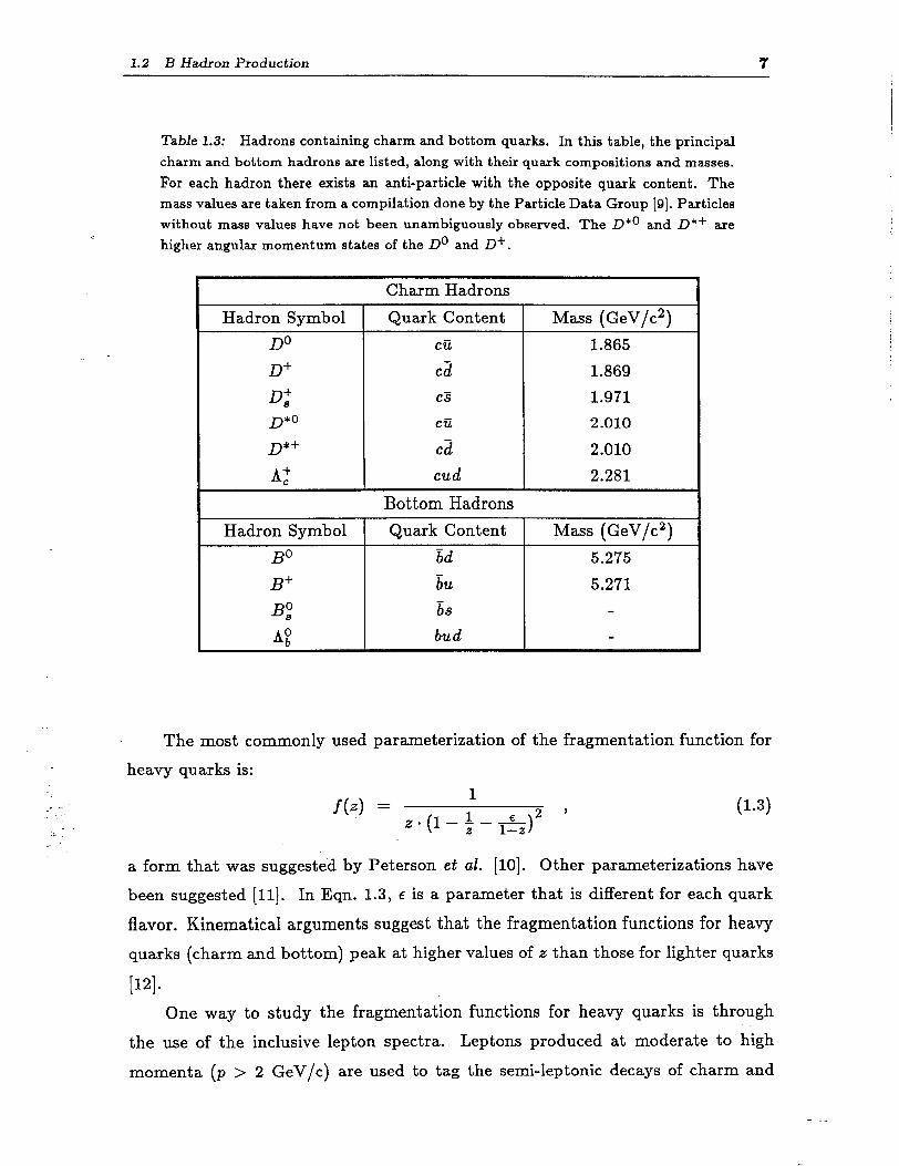
Table 1.3: Hadrons containing charm and bottom quarks. In this table, the principal charm and bottom hadrons are listed, along with their quark compositions and masses. For each hadron there exists an anti-particle with the opposite quark content. The mass values are taken from a compilation done by the Particle Data Group [Q]. Particles without mass values have not been unambiguously observed. The D*O and D*+ are higher angular momentum states of the Do and D+.
Hadron Symbol
DO
D+
0;: D*O
D*+
c
Hadron Symbol B0 B+
B,O Aif
Charm Hadrons Quark Content
Cti
C;i
CS
CiSi
C2
cud
Bottom Hadrons Quark Content
&d IiU
6s bud
Mass ( GeV/c2) 1.865 1.869 1.971 2.010
2.010 2.281
Mass ( GeV/c2) 5.275 5.271
The most commonly used parameterization of the fragmentation function for
heavy quarks is:
f( 1 1 z =
z*(l- p- &)2 9 (13) .
a form that was suggested by Peterson et al. [lo]. Other parameterizations have
been suggested [Ill. In Eq n. 1.3, E is a parameter that is different for each quark
flavor. Kinematical arguments suggest that the fragmentation functions for heavy quarks (charm and bottom) peak at higher values of z than those for lighter quarks
1 21 1. One way to study the fragmentation functions for heavy quarks is through
the use of the inclusive lepton spectra. Leptons produced at moderate to high
momenta (p > 2 GeV/c) are used to tag the semi-leptonic decays of charm and
8 Introduction
Figure 1.3: Quark fragmentation. This figure represents the phenomological picture of quark fragmentation as incorporated into the Monte Carlo. The quark Q is fragmented into the hadron H by the production of a qij pair. The use of the Monte Carlo is discussed in Chapter 3.
bottom hadrons. The measured momentum spectrum of the leptons can be used
to infer the average hadron energy, and thus the mean z (written here as < z > )
of the fragmentation function. In addition, since bottom and charm semi-leptonic
decays can be partially separated on the basis of the lepton transverse momentum,
one can measure < z > for bottom and charm separately. This technique is used in
this thesis to determine < z > for the bottom fragmentation function.
Inclusive leptons have been used to measure < xc > and < q, > by a number
of groups at the PEP and PETRA accelerators. These results are summarized
in review articles by Bethke [13] and in a recent measurement by the JADE group
[ 141. The results from different experiments are in good agreement with one another,
giving an < zc > = 0.63 k 0.04 and an < xb > = 0.80 rt 0.05. In addition, the
inclusive lepton analyses determine the semi-leptonic charm and bottom branching
ratios.
The determination of the heavy quark fragmentation functions by the means
of the inclusive lepton spectra has a number of systematic problems. Since C and
B hadrons are not fully reconstructed, the determination of their fragmentation
functions is somewhat subject to assumptions made on the momentum distribution
and multiplicity of the remaining particles from their decay. In addition, the
lepton signal does not completely separate charm and bottom decays and there is
a significant background to the signal from mis-identified hadrons and non-prompt
leptons.
1.2 B Hadron Production 9
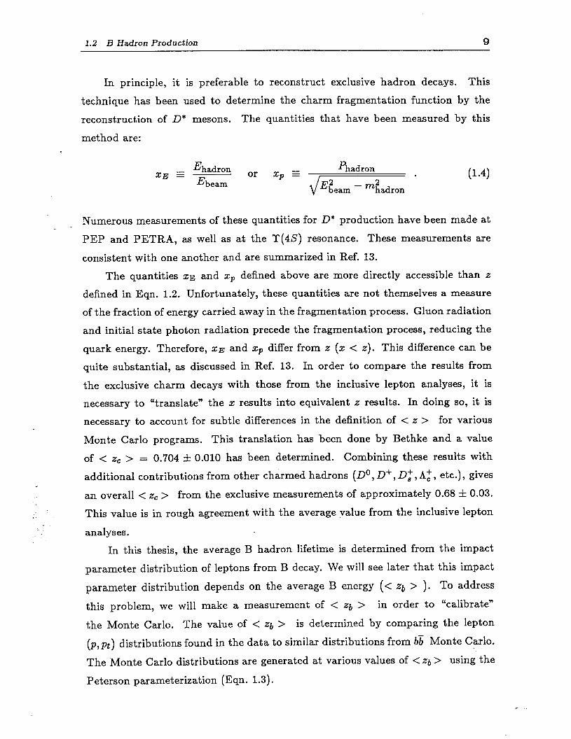
In principle, it is preferable to reconstruct exclusive hadron decays. This
technique has been used to determine the charm fragmentation function by the
reconstruction of D* mesons. The quantities that have been measured by this
method are:
XE = Ehadron or
Ebeam ( 4 1.
Numerous measurements of these quantities for D* production have been made at
PEP and PETRA, as well as at the Y’(4S) resonance. These measurements are
consistent with one another and are summarized in Ref. 13. The quantities XE and xp defined above are more directly accessible than z
defined in Eqn. 1.2. Unfortunately, these quantities are not themselves a measure
of the fraction of energy carried away in the fragmentation process. Gluon radiation
and initial state photon radiation precede the fragmentation process, reducing the
quark energy. Therefore, XE and xp differ from z (x < z). This difference can be
quite substantial, as discussed in Ref. 13. In order to compare the results from
the exclusive charm decays with those from the inclusive lepton analyses, it is
necessary to “translate” the x results into equivalent z results. In doing so, it is
necessary to account for subtle differences in the definition of < z > for various
Monte Carlo programs. This translation has been done by Bethke and a value
of < zc > = 0.704 & 0.010 has been determined. Combining these results with
additional contributions from other charmed hadrons (Do, D+, Dt, AZ, etc.), gives
an overall < zc > from the exclusive measurements of approximately 0.68 AI 0.03.
This value is in rough agreement with the average value from the inclusive lepton
analyses.
In this thesis, the average B hadron lifetime is determined from the impact
parameter distribution of leptons from B decay. We will see later that this impact
parameter distribution depends on the average B energy (< ~b > ). To address
this problem, we will make a measurement of < zb > in order to “calibrate”
the Monte Carlo. The value of < xb > is determined by comparing the lepton
(p, pt) distributions found in the data to similar distributions from bb Monte Carlo.
The Monte Carlo distributions are generated at various values of < xb > using the
Peterson parameterization (Eqn. 1.3).
10 Introduction
Because C hadrons are more relativistic than B hadrons, the impact
parameter distribution for leptons from charm decay is significantly less sensitive
to fragmentation than that for bottom. For this reason, we choose not to measure
< zc > , and instead assume a world average value of 0.68.
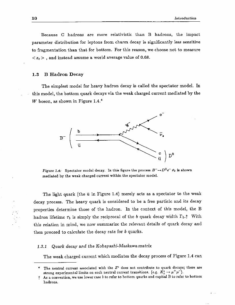
1.3 B Hadron Decay
The simplest model for heavy hadron decay is called the spectator model. In
- this model, the bottom quark decays via the weak charged current mediated by the
VV boson, as shown in Figure 1.4.*
B-
Figure 1.4: Spectator model decay. In this figure the process B--*Doe- y’e is shown mediated by the weak charged current within the spectator model.
The light quark (the ti in Figure 1.4) merely acts as a spectator to the weak
decay process. The heavy quark is considered to be a free particle and its decay
properties determine those of the hadron. In the context of this model, the B
hadron lifetime Q, is simply the reciprocal of the b quark decay width I’& With
this relation in mind, we now summarize the relevant details of quark decay and
then proceed to calculate the decay rate for b quarks.
1.3.1 Quark decay and the Xobayashi-Maskawamatrix
The weak charged current which mediates the decay process of Figure 1.4 can
* The neutral current associated with the 2’ does not contribute to quark decays; there are strong experimental limits on such neutral current transitions. (e.g. Ki -+ ,z’p-).
t As a convention, we use lower case b to refer to bottom quarks and capital B to refer to bottom hadrons.
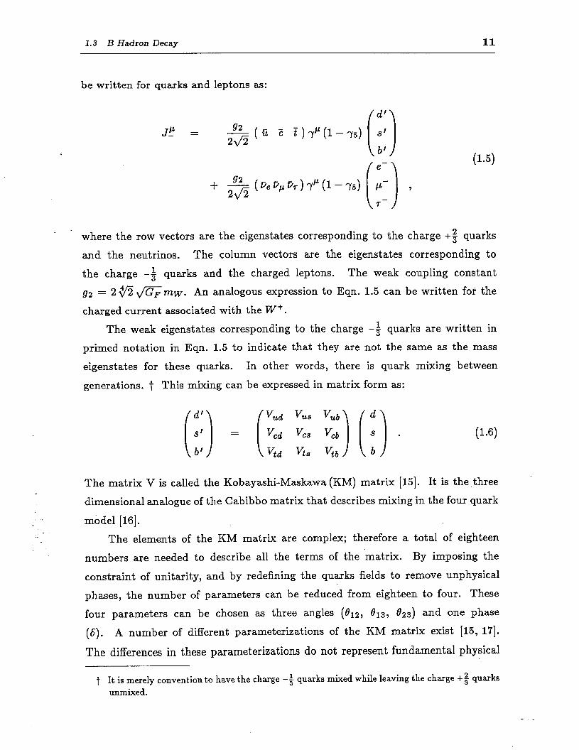
1.3 B Hadron Decay 11
be written for quarks and leptons as:
d’
JF = 92 2Jz
(a 72 Z)qC"(l-y5) 0 s' b’
0 e- (15) .
!?2 +- 2fi
(QdpQr)ryCl(1-75) p- ,
r-
_ - where the row vectors are the eigenstates corresponding to the charge +$ quarks
and the neutrinos. The column vectors are the eigenstates corresponding to
the charge -$ quarks and the charged leptons. The weak coupling constant
g2 = 2fimrnw. An analogous expression to Eqn. 1.5 can be written for the
charged current associated with the W+.
The weak eigenstates corresponding to the charge --$ quarks are written in
primed notation in Eqn. 1.5 to indicate that they are not the same as the mass
eigenstates for these quarks. In other words, there is quark mixing between
generations. t This mixing can be expressed in matrix form as:
The matrix V is called the Kobayashi-Maskawa (KM) matrix [15]. It is the three
dimensional analogue of the Cabibbo matrix that describes mixing in the four quark
model [ 161. The elements of the KM matrix are complex; therefore a total of eighteen
numbers are needed to describe all the terms of the matrix. By imposing the
constraint of unitarity, and by redefining the quarks fields to remove unphysical
phases, the number of parameters can be reduced from eighteen to four. These
four parameters can be chosen as three angles (612, 013, 023) and one phase
(6). A number of different parameterizations of the KM matrix exist [15, 171.
The differences in these parameterizations do not represent fundamental physical
t It is merely convention to have the charge -$ quarks mixed while leaving the charge +$ quarks unmixed.
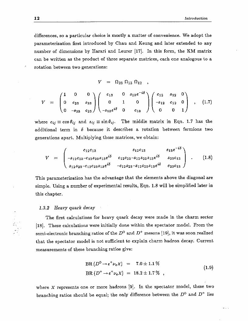
12 Introduction
differences, so a particular choice is mostly a matter of convenience. We adopt the
parameterization first introduced by Chau and Keung and later extended to any
number of dimensions by Harari and Leurer [17]. In this form, the KM matrix
can be written as the product of three separate matrices, each one analogous to a r: rotation between two generations:
v = n23 a13 %2 >
where cij z cos Bij and sij E sin Q. The middle matrix in Eqn. 1.7 has the
additional term in 6 because it describes a rotation between fermions two
generations apart. Multiplying these matrices, we obtain:
clZc13 slZc13
v = -slZc23-clZs23s13e is
cl2c23--+12s23sl3e i6
(18) .
~12~23--~12~23~13~ is
-cl2s23-s12c23sl3e i6
This parameterization has the advantage that the elements above the diagonal are
simple. Using a number of experimental results, Eqn. 1.8 will be simplified later in
this chapter.
1.3.2 Heavy quark decay
-_ The first calculations for heavy quark decay were made in the charm sector
[ 181. These calculations were initially done within the spectator model. From the
semi-electronic branching ratios of the Do and D+ mesons [ 191, it was soon realized
that the spectator model is not sufficient to explain charm hadron decay. Current
measurements of these branching ratios give:
BR (Do + e’v&) = 7.0 xt 1.1%
BR (D+ +e+v,X) = 18.2 & 1.7 % , (19) .
where X represents one or more hadrons [9]. In the spectator model, these two
branching ratios should be equal; the only difference between the Do and .D+ lies

1.3 B Hadron Decay 13
in their respective spectator quarks. There has been considerable effort made
to understand charm hadrons by including non-spectator diagrams (such as the
annihilation, exchange and Penguin diagrams) [20], and by the development of
models for exclusive charm decay [21]. Although the subject of charm decays is a i fascinating one, our main concern is with the decays of bottom hadrons.
1.3.3 Bottom quark decay
In the absence of generation mixing (i.e. V diagonal), quarks would couple
only to their doublet partners. This situation would result in a stable b quark since
it is lighter than its top quark partner. In the KM scheme, the bottom quark can
decay into the lighter u and c quarks, with amplitudes proportional to the terms
Vub and Vca respectively. These b quark decays are illustrated in Figure 1.5.
1-
b
’ q
Figure 1.5: Contributions to b quark decay. The amplitude for each diagram is proportional to the KM matrix terms Vub and Vcb respectively. The qq pair produced can be any of the quark combinations present in the KM matrix.
The total b quark decay rate can then be written as the sum of contributions
from (b-+ U) and (b+ c) transitions:
rtot = c w-4 . q=u,c
('1.10)
The decay rate for each particular quark transition (b + q) can be broken up into
semi-leptonic and hadronic parts:
r@-+q) = rsl(b-V) + rhad(b-)q) l (1.11)
14 Introduction
Let us first consider rSl (b + q). The matrix element for this process can be written:
(1.12)
-: This matrix element is similar to that for muon decay; therefore after squaring it
and integrating over phase space we obtain:
Lz(b+a) = (1.13)
The first factor in Eqn. 1.13 corresponds to the muon decay rate with the b quark
mass substituted for the muon mass. The second factor is the appropriate KM
matrix element and the last one is the phase space factor:
I(4 = l-8~2+&~8-24~41n~ , (1.14)
for E f mq/mb. The factor I(E) is close to unity for muon decay and (b+ u) transi-
tions, but is approximately 0.5 for (b -+ c) transitions (E - 0.3). Returning to Eqn. 1.11, we note that the hadronic part for (b+ q) transitions is
simply 3 times rsl given in Eqn. 1.13. The factor of 3 comes about because of color.
Therefore, considering the possible lepton and quark combinations* from the W
decay, and neglecting phase space effects, the decay rates for the (b + q) transition
are in the ratio:
eve : /.~p : TUT : ad : ii% = 1: 1 : 1 : 3 : 3 . (1.15)
This simple picture’of b quark decay predicts a semi-leptonic branching ratio of i
(- 11%) for each lepton type.
1.3.4 Improvements to the spectator decay model
To improve the calculation of the b quark decay rate, we now consider the
* Although all quark combinations connected by an element of the KM matrix are possible, those combinations connected by a diagonal element (Cabibbo-favored) have much larger decay rates than the off-diagonal combinations (Cabibbo-supressed).

1.3 B Hadron Decay 15
following refinements to the spectator model:
0 First order gluon radiation. 0 Short distance QCD effects.
0 Mass effects from the final state particles. ,
The first refinement includes gluon radiation effects that are soft in comparison
with the b quark mass. These effects lower the predicted decay rate for both the
hadronic and semi-leptonic modes. The second category contains gluon effects that
_ are hard in comparison with the b quark mass, but are soft in comparison with the
IV (e.g. gluon exchange). These effects substantially increase the hadronic decay
rate but leave the semi-leptonic rate untouched. The third refinement lowers the
predicted decay rate for both the hadronic and semi-leptonic modes.
Gluon radiation:
Two diagrams contributing to first order gluon radiation are illustrated in
Figure 1.6. These diagrams were originally studied in the context of charm decay
[22]. In these studies, it was observed that the QCD corrections for heavy quark
decay can be easily related to the QED corrections for muon decay [23]. In this
comparison, the following substitution is made:
4 a+-o!Q.
3
The quantity a, is given by:
12 7r _ _- I - as = (33 - 2nf) ln(mi/h2) ’
(1.16)
(1.17)
where nf is the number bf effective quark flavors, rnb is the mass of the bottom
quark, and A is the QCD renormalization point. For typical values of the parameters
(nf = 4, rnb = 4.8 GeV/c2, and A = 0.2 GeV/c2), one gets a value a, = 0.24.
Using the results given in Ref. 23, the corrections to the b quark semi-leptonic
rate due to first order gluon radiation have been calculated [24]. These corrections
modify Eqn. 1.13 to become:
(1.18)
16 Introduction
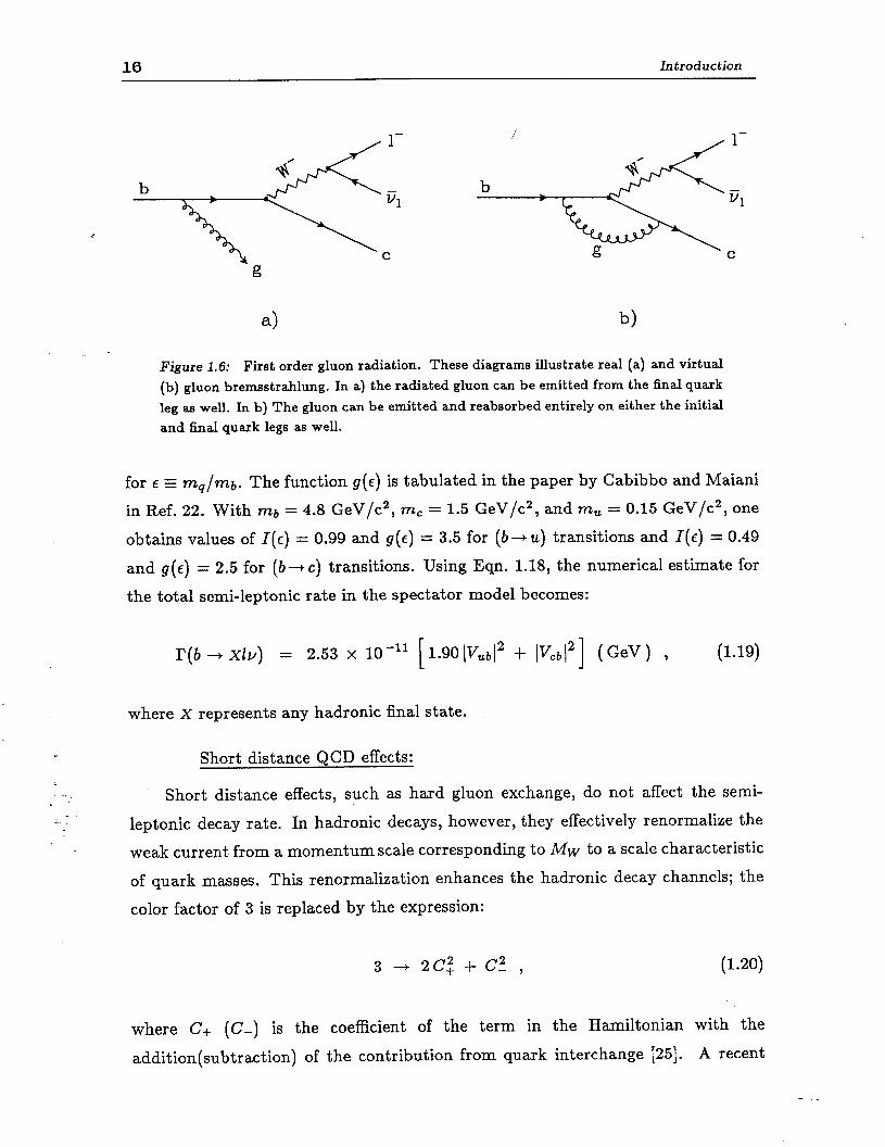
b
4 b)
Figure 1.6: First order gluon radiation. These diagrams illustrate real (a) and virtual (b) gluon bremsstrahlung. In a) the radiated gluon can be emitted from the final quark leg as well. In b) The gluon can be emitted and reabsorbed entirely on either the initial and final quark legs as well.
for E = mp/ma. The function g(e) is tabulated in the paper by Cabibbo and Maiani
in Ref. 22. With rnb = 4.8 GeV/c2, m, = 1.5 GeV/c2, and mu = 0.15 GeV/c2, one
obtains values of I(E) = 0.99 and g(E) = 3.5 for (b-w) transitions and I(E) = 0.49
and iI(E) = 2.5 for (b + c) transitions. Using Eqn. 1.18, the numerical estimate for
the total semi-leptonic rate in the spectator model becomes:
I’(b + XZY) = 2.53 x lo-l1 [ 1.90 IV&l2 + IVcb12] ( GeV ) 9 (1.19)
where X represents any hadronic final state.
Short distance QCD effects:
_r --
- -1. Short distance effects, such as hard gluon exchange, do not affect the semi-
leptonic decay rate. In hadronic decays, however, they effectively renormalize the
weak current from a momentum scale corresponding to Mw to a scale characteristic
of quark masses. This renormalization enhances the hadronic decay channels; the
color factor of 3 is replaced by the expression:
3*2cf+c2, (1.20)
where C+ (C-) is the coefficient of the term in the Hamiltonian with the
addition(subtraction) of the contribution from quark interchange [25]. A recent
1.3 B Hadron Decay 17
estimate [26] gives C+ - 0.8 and C- - 1.5. This leads to an 18 % enhancement in
the hadronic decay rate.
Mass effects:
c Until now we have considered the quarks and leptons produced at the Fiv decay
vertex to be massless. That assumption is reasonable in the case of (eve),(puP),
and (ad) final states. The production of (r, v~) and (ES) states will be suppressed
due to phase space. These effects have been calculated [27]; combining them with
- . the short distance QCD effects, the relative decay ratios of Eqn. 1.15 become:
eu, : pup : ruT : iid : Zs = 1.0 : 1.0 : 0.2 : 3.5 : 0.8 . (1.21)
#With these corrections we now expect a semi-leptonic (electron and muon)
branching ratio of approximately 15 %. The current world average is 12.1 I!I 0.8 % [14]. The fact that the measured value of the semi-leptonic branching ratio is lower
that the theoretical estimate is seen as evidence for further enhancement of the
hadronic decay rate. In any case, from the experience with charm decays, it is
believed that non-spectator effects in semi-leptonic decays are considerably smaller
than those in hadronic decays. Therefore, the total b quark decay rate can be
determined most accurately from the expression:
hot = I’(b + xly)
BR(b + xly) ’ (1.22)
-. _ . . z
where we use the calculated semi-leptonic decay rate (Eqn. 1.18) and the measured
value of the semi-leptonic branching ratio.
1.3.5 Beyond the spectator decay model
Even though we believe the estimate of the semi-leptonic decay rate from the
spectator model to be reliable, there is still a strong dependence in Eqn. 1.18 on
mb. This “bare quark” mass is uncertain to the level of 200-300 MeV/c2 , leading
to a sizable uncertainty in the calculation of I’.
One way to reduce this uncertainty is to use the well measured B meson ma+ to help determine mb. The bare quark mass can be related to the mass of the B meson
by examining the B lepton spectrum in the context of the spectator decay model
18 Introduction
[28]. In this comparison the effects of soft gluon radiation, the mass of the spectator
quark, and Fermi motion within the meson have been taken into account. The result
of such a comparison with the CLEO data yields a value rnb = 4.95 3~ 0.04 GeV/c2
[29]. Using this mass in Eqn. 1.18 gives a value for the semi-leptonic decay rate:
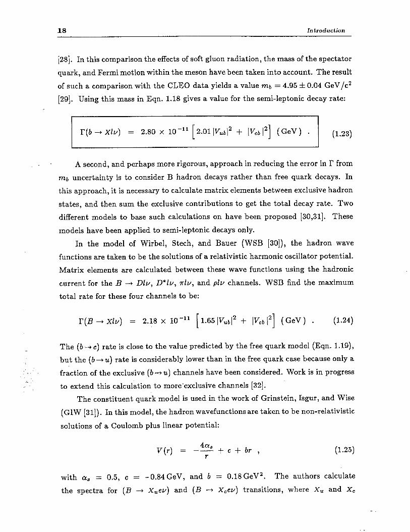
I’(b + xiv) = 2.80 x lo-l1 [2WV~b/2 + IVcb 12] (GeV) . (1.23)
A second, and perhaps more rigorous, approach in reducing the error in I’ from
rnb uncertainty is to consider B hadron decays rather than free quark decays. In
this approach, it is necessary to calculate matrix elements between exclusive hadron
states, and then sum the exclusive contributions to get the total decay rate. Two
different models to base such calculations on have been proposed [30,31]. These
models have been applied to semi-leptonic decays only.
In the model of Wirbel, Stech, and Bauer (WSB [3O]), the hadron wave
functions are taken to be the solutions of a relativistic harmonic oscillator potential.
Matrix elements are calculated between these wave functions using the hadronic
current for the B + Dlv, D*Zv, XZY, and plv channels. WSB find the maximum
total rate for these four channels to be:
r(B + xlu) 2.18 x 10-l' [ 1.65 ILb12 + pica I21 (GeV) . (1.24)
The (b --+ c) rate is close to the value predicted by the free quark model (Eqn. 1.19),
but the (b + u) rate is considerably lower than in the free quark case because only a
fraction of the exclusive (b -+ u) channels have been considered. Work is in progress
to extend this calculation to more-exclusive channels [32].
The constituent quark model is used in the work of Grinstein, Isgur, and Wise
(GIW [31]). In th is model, the hadron wavefunctions are taken to be non-relativistic
solutions of a Coulomb plus linear potential:
v(r) = -+ + c + br , (1.25)
with a, = 0.5, c = -0.84 GeV, and b = 0.18 GeV2. The authors calculate
the spectra for (B -+ X,ev) and (B -+ &ev) transitions, where xu and xc
1.3 B Hadron Decay 19
are mesons made from UZ and CZ combinations respectively. They find that the
(B --+ X,ev) transitions are effectively saturated by production of D and D’ mesons,
in agreement with experimental observation. For the (B + X,ev) transitions, the
total rate is not saturated by the lowest lying states; therefore an uncertainty in ,
the overall normalization of 20 % is assigned, and GIW suggest using the free quark
model prediction for this rate.
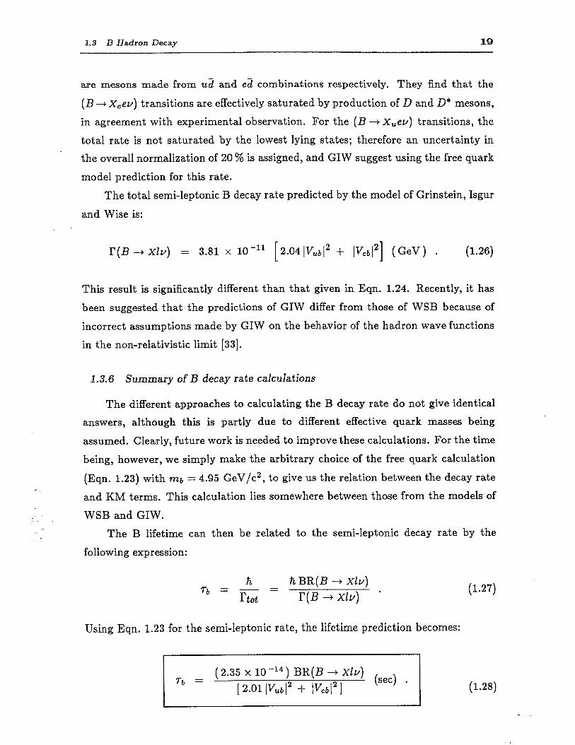
The total semi-leptonic B decay rate predicted by the model of Grinstein, Isgur
and Wise is:
I’(B + xiv) = 3.81 x lo--l1 [ 2.04 ITJILb12 + I&12] (GeV) . (1.26)
This result is significantly different than that given in Eqn. 1.24. Recently, it has
been suggested that the predictions of GIW differ from those of WSB because of
incorrect assumptions made by GIW on the behavior of the hadron wave functions
in the non-relativistic limit [33].
1.3.6 Summary of B decay rate calculations
The different approaches to calculating the B decay rate do not give identical
answers, although this is partly due to different effective quark masses being
assumed. Clearly, future work is needed to improve these calculations. For the time
being, however, we simply make the arbitrary choice of the free quark calculation
(Eqn. 1.23) with rnb = 4.95 GeV/c 2, to give us the relation between the decay rate
and KM terms. This calculation lies somewhere between those from the models of
WSB and GIW.
The B lifetime can then be related to the semi-leptonic decay rate by the
following expression:
Ii 73 = - = fi BR(B + XZY)
hot I'(B -+ xb) l
Using Eqn. 1.23 for the semi-leptonic rate, the lifetime prediction becomes:
Tb = (2.35 x 10 -14) BR(B + XZY)
[ 2.01 lvz,b12 + l&-,12] (sec) l
(1.27)
(1.28)
20 Introduction
The measured value of rb can be used to constrain the KM elements IV&, I and IVcal.
I.4 Testing the KM Model
c The direct constraint on elements of the Kobayashi-Maskawa matrix from
measurement of the B lifetime is shown in Eqn. 1.28. In general, however, the B
lifetime is only one of a number of key measurements that can be used to test the KM
model. The problems of accommodating these measurements within the framework
_ - of a unitary KM matrix is the subject of much study [34]. This subject is of great
importance for a number of reasons. Failure of the KM matrix to obey unitarity
might signal new physics or the presence of a fourth generation. In addition, it
is hoped that quark mixing provides an explanation for CP violation within the
standard model. Finally, careful study of the quark couplings might shed light
on possible relations between the quark masses and the matrix elements, so as to
reduce the number of free parameters in the model [35].
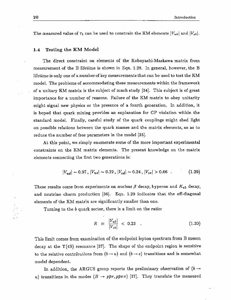
At this point, we simply enumerate some of the more important experimental
constraints on the KM matrix elements. The present knowledge on the matrix
elements connecting the first two generations is:
lVudl - 0.97, IV,,l - 0.22, lVcdl - 0.24, IVesI > 0.66 . (1.29)
These results come from experiments on nuclear ,O decay, hyperon and Ke3 decay,
and neutrino charm production 1361. Eqn. 1.29 indicates that the off-diagonal
elements of the KM matrix are significantly smaller than one.
i - Turning to the b quark s.ector, there is a limit on the ratio:
R = - Iv I ub
Iv I cb < 0.23 . (1.30)
This limit comes from examination of the endpoint lepton spectrum from B meson
decay at the Y(4S) resonance 1371. The shape of the endpoint region is sensitive
to the relative contributions from (b + U) and (b -+ c) transitions and is somewhat
model dependent.
In addition, the ARGUS group reports the preliminary observation of (b +
U) transitions in the modes (B + pp7rlr, pp7~) [37]. They translate the measured
1.4 Testing the KM Model 21
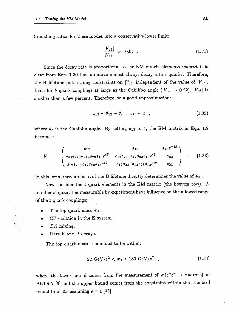
branching ratios for these modes into a conservative lower limit:
-2 > 0.07 . Iv I IV I cb
(1.31)
c Since the decay rate is proportional to the KM matrix elements squared, it is
clear from Eqn. 1.30 that b quarks almost always decay into c quarks. Therefore,
the B lifetime puts strong constraints on ]v&] independent of the value of ]I&$
Even for b quark couplings as large as the Cabibbo angle (I&] - 0.22)) I&l is . smaller than a few percent. Therefore, to a good approximation:
s12 - e12 -& ; Cl3 -1 7 (1.32)
where 8, is the Cabibbo angle. By setting ~13 to 1, the KM matrix in Eqn. 1.8
becomes:
Cl2 s12 s13e -is
v = -s12c23-c12s23s13e is
cl2c23--sl2s23sl3e ii5
823 . (1.33)
s12s23--c12c23s13e i6
-cl2s23--sl2c23sl3e iS
c23
In this form, measurement of the B lifetime directly determines the value of ~23.
Now consider the t quark elements in the KM matrix (the bottom row). A number of quantities measurable by experiment have influence on the allowed range
of the t quark couplings:
0 The top quark mass mt.
0 CP violation in the K system.
0 BB mixing.
l Rare K and B decays.
The top quark mass is bounded to lie within:
22 GeV/c2 < mt < 180 GeV/c2 , (1.34)
where the lower bound comes from the measurement of 0 (e+e- + Hadrons) at
PETRA [9] and the upper bound comes from the constraint within the standard
model from Ar assuming p = 1 [38].
22 Introduction
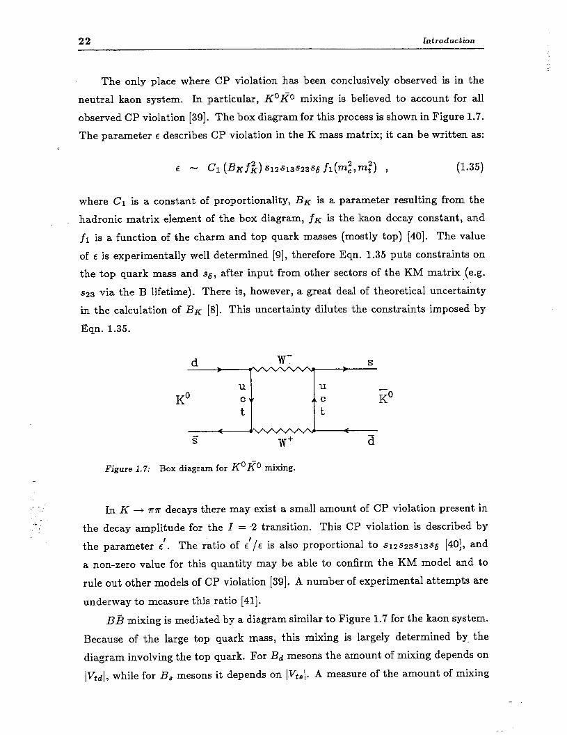
The only place where CP violation has been conclusively observed is in the
neutral kaon system. In particular, K”@ mixing is believed to account for all
observed CP violation [39]. The box diagram for this process is shown in Figure 1.7.
The parameter E describes CP violation in the K mass matrix; it can be written as:
E - cl (B&)sl2S13S23S~ fl(m:,'$) I) (1.35)
where cr is a constant of proportionality, BK is a parameter resulting from the
_ hadronic matrix element of the box diagram, fK is the kaon decay constant, and
fr is a function of the charm and .top quark masses (mostly top) [do]. The value
of E is experimentally well determined [9], therefore Eqn. 1.35 puts constraints on
the top quark mass and ~6, after input from other sectors of the KM matrix (e.g.
~23 via the B lifetime). There is, however, a great deal of theoretical uncertainty
in the calculation of BK [8]. Th is uncertainty dilutes the constraints imposed by
Eqn. 1.35.
Figure 1.7: Box diagram for K°Ko mixing.
.
.: In K -N 7r7r decays there may exist a small amount of CP violation present in
the decay amplitude for the I = -2 transition. This CP violation is described by
the parameter E’. The ratio of e’/e is also proportional to s12s23s13s~ [40], and
a non-zero value for this quantity may be able to confirm the KM model and to
rule out other models of CP violation [39]. A number of experimental attempts are
underway to measure this ratio [41].
BB mixing is mediated by a diagram similar to Figure 1.7 for the kaon system.
Because of the large top quark mass, this mixing is largely determined by, the
diagram involving the top quark. For Bd mesons the amount of mixing depends on
IVtdl, while for B, mesons it depends on IV& A measure of the amount of mixing
1.5 Analysis 0 bjec tive 23
is provided by the parameter z, defined as the ratio of the BL - Bs mass difference
to the B decay rate. For B& mixing, this parameter can be expressed as:
AM xd = - r - c2 rb 6;s (BBfB) Ivtd12f2(m:) > (1.36)
where C2 is a constant of proportionality, BB and fB are analogous to BK and fK
in the kaon system, and f2 is a function of the top quark mass [42]. Just as in the
expression for E, there is a strong dependence in Eqn. 1.36 on mt.
Experimentally, mixing can be observed by looking at dilepton Bd& events.
The strength of the mixing is measured by a parameter rd, the ratio of like sign to
unlike sign dilepton events. This parameter can be expressed in terms of zd by the
relation: 4 ?-d = -
2; + 2 = 0.22 zk 0.09 zt 0.04 . (1.37)
The experimental value for rd comes from a recent measurement by the ARGUS
group [43]. S ince II&l is expected to be much larger than I&d], Eqn. 1.37 implies
that rs - 1. The ARGUS results are consistent with a previous result from the
UAl group [44].
Limits on rare decay modes of K and B mesons also help to constrain the
KM matrix [45]. In particular, the rate for the process K+ -+ ?r+v~ puts similar
constraints as E’/E on the KM model [46].
1.5 Analysis Objective
_ ._ : - . . .
Before 1983, it was conventional to assume that (b + c) couplings were
approximately of the same magnitude as the coupling between the first two
generations ( lVbcl - 8,). These ass_umptions lead to a predicted B lifetime of - 0.07
ps, too short to be measured by existing experiments. Conventional wisdom proved
wrong. In the summer of 1983, the MAC and Mark II groups reported the first B
lifetime measurements [47,48]:
Tb = 1.80 zt 0.60 rt 0.40 ps (MAC) , (1.38)
rb = 1.20 t;*;; . III 0.30~s (Mark II) ,
where the first error is statistical and the second systematic. These measured
lifetimes were some twenty times longer than originally predicted, indicating that
24 Introduction
the second and third generations are much more weakly coupled than are the first
two. A number of other measurements have followed those listed in Eqn. 1.38 and
are summarized in Chapter 10.
The primary objective of this thesis is to measure the B lifetime and
significantly reduce the error on the measurement (both statistical and systematic).
The first critical step in the lifetime measurement is the isolation of a sample of
events that are enriched in B hadron production. This enrichment is most reliably
done by selecting events containing a high transverse momentum lepton [49]. A B
purity of approximately 65 % is obtained in this manner (an amount considerably
better than l/11, the fraction of produced b6 pairs).
The second step in the analysis is to measure the displacement from the origin
of tracks in these events coming from B hadrons. In principle, one would like to
measure the B decay length. Unfortunately, full reconstruction of B hadrons is
quite difficult. This difficulty arises partly because of the large number of tracks in
a typical event and partly because of the neutral particles that are often produced
in B decay and remain undetected. For this reason, in this thesis, only charged
particles reliably known to have come from B hadron decay are used in the lifetime
determination.
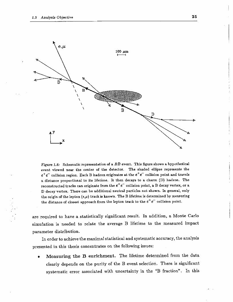
A schematic representation of a BB event is shown in Figure 1.8. In addition to
the tracks from B decay, there are tracks from the primary (e+e-) interaction point
and from secondary charm decays. Therefore the only track known with confidence
to have originated from B hadron decay is the high pt lepton. The distance of
closest approach (impact parameter) of this lepton track measured relative to the
B production point contains information about the parent lifetime.
The high pt lepton is used to provide a measure of the B lifetime as well as to
enrich the sample. Therefore we measure the B lifetime averaged over the various
types of B hadrons produced and weighted by the relative semi-leptonic branching
ratios for these hadrons.
For a B lifetime in the vicinity of 1 ps, the average lepton impact parameter is
approximately 145 pm. As discussed in Chapter 2, the addition of a high precision
inner drift chamber (the Vertex Chamber) greatly enhanced the ability of the
Mark II detector to measure such short distances. Even so, with an experimental
resolution that is only comparable to the lifetime effect, a large number of events
1.5 Analysis 0 bjec tive 25
Figure 1.8: Schematic representation of a BB event. This figure shows a hypothetical event viewed near the center of the detector. The shaded ellipse represents the e+e- collision region. Each B hadron originates at the e+e- collision point and travels a distance proportional to its lifetime. It then decays to a charm (D) hadron. The reconstructed tracks can originate from the e+e- collision point, a B decay vertex, or a D decay vertex. There can be additional neutral particles not shown. In general, only the origin of the lepton (e,p) track is known. The B lifetime is determined by measuring the distance of closest approach from the lepton track to the e+e- collision point.
are required to have a statistically significant result. In addition, a Monte Carlo
simulation is needed to relate the average B lifetime to the measured impact
parameter distribution.
In order to achieve the maximal statistical and systematic accuracy, the analysis
presented in this thesis concentrates on the following issues:
l Measuring the B enrichment. The lifetime determined from the data
clearly depends on the purity of the B event selection. There is significant
systematic error associated with uncertainty in the “B fraction”. In this
26 Introduction
thesis, a separate analysis of inclusive leptons is done to measure this fraction
in the data.
0 Determining the average B hadron energy. The relationship between
the impact parameter distribution and the corresponding lifetime depends
on the average B hadron energy. In this analysis, we determine this average
energy by measuring < x > of the B fragmentation function.
l Understanding the impact parameter resolution. Improvements in
the charged particle tracking can lead to a higher efficiency and resolution
for the reconstruction of tracks. In addition, an understanding of the shape
and tails of the resolution function (by measuring it in the data) is needed to
have confidence in the lifetime fit and to reduce the systematic errors caused
by resolution effects.
1.6 Thesis Outline
In Chapter 2, the experimental apparatus used to make the lifetime
measurement is introduced. A discussion of the event reconstruction procedure
and the Monte Carlo follows in Chapter 3, while Chapter 4 is devoted to a
careful study of the Vertex Chamber resolution. The identification and analysis
of inclusive leptons in hadronic events are outlined in Chapters 5 and 6. The use
of the impact parameter technique and the resulting lifetime determination are
presented in Chapter 7 and 8, respectively. Checks on the analysis procedure and
the estimation of systematic errors are presented in Chapter 9. The final chapter
contains a summary of the results, the theoretical implications, and a comparison
with other experiments. The. appendices document some of the analysis details.
Chapter 2
Experimental Apparatus
2.1 The PEP Storage Ring
The data used in this thesis were taken with the Mark II detector at the
PEP (Positron Electron Project) storage ring. PEP is a large positron-electron
colliding beam facility with a circumference of 2.2 km, located at the Stanford
Linear Accelerator Center (SLAC) [50]. F g i ure 2.1 illustrates the location of the
PEP ring and the Mark II detector on the SLAC site.
In the PEP ring, three bunches of electrons and positrons circulate, colliding
every 2.4 ps at each of the six interaction regions. The e+e- collision region
(the interaction point) has an effective rms width of approximately 4OOpm in the
horizontal (z) direction, 7Opm in the vertical (y) d irection, and 1.5 cm in the
direction parallel to the beams (2). The typical luminosity seen by the Mark II at
PEP was - 1 x 1031 crnm2 see-l ( = 0.01 nb-l set-l ). The integrated luminosity
over the years 1981-1984 was approximately 206 pb-’ .
2.2 The Mark II Detector: Overview
The Mark II detector was designed and built by a collaboration of scientists
from SLAC and the Lawrence Berkeley Laboratory (LBL). Completed in 1977, the
Mark II first operated at the SPEAR storage ring at SLAC and accumulated data
from e+e- annihilations at center of mass energies between 3.0 and 7.5 GeV.
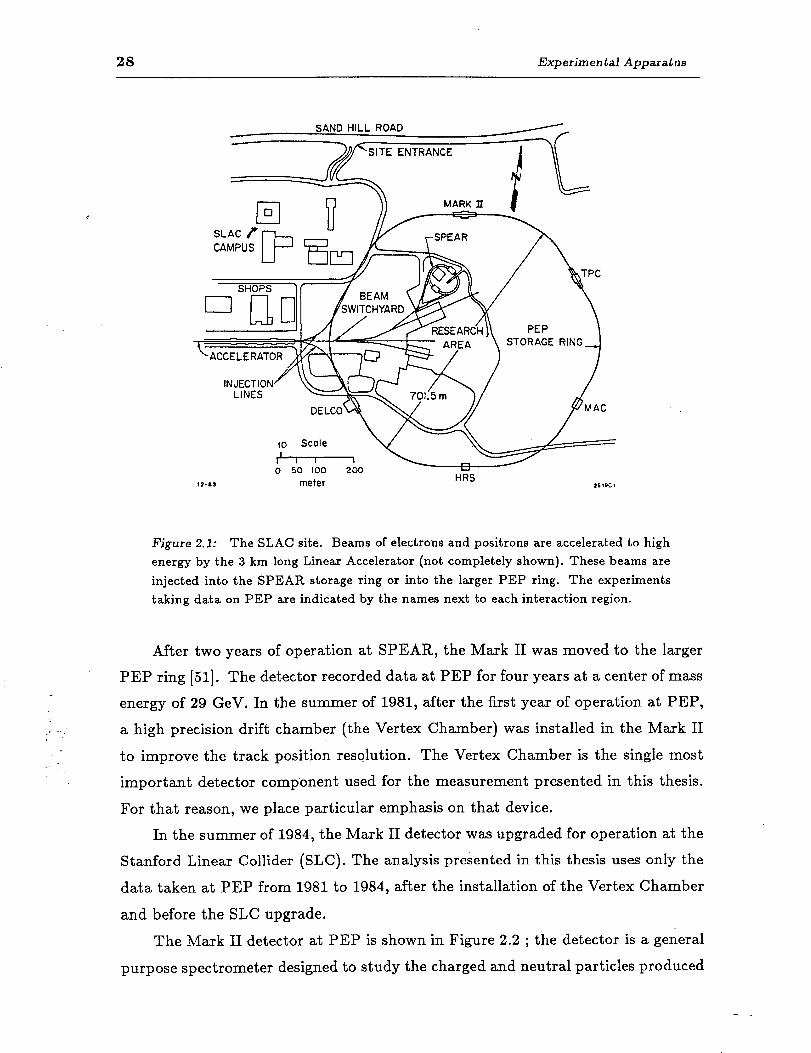
28 Experimental Apparatus
SAND HILL ROAD
SITE ENTRANCE
TPC ” 10 Scale I’ I 1 1 0 50 100 200 . *-a
meter HKS ZS!OCl
Figure 2.1: The SLAC site. Beams of electrons and positrons are accelerated to high energy by the 3 km long Linear Accelerator (not completely shown). These beams are injected into the SPEAR storage ring or into the larger PEP ring. The experiments taking data on PEP are indicated by the names next to each interaction region.
After two years of operation at SPEAR, the Mark II was moved to the larger
PEP ring [51]. The detector recorded data at PEP for four years at a center of mass
energy of 29 GeV. In the summer of 1981, after the first year of operation at PEP,
a high precision drift chamber (the Vertex Chamber) was installed in the Mark II
to improve the track position resolution. The Vertex Chamber is the single most
important detector component used for the measurement presented in this thesis.
For that reason, we place particular emphasis on that device.
In the summer of 1984, the Mark II detector was upgraded for operation at the
Stanford Linear Collider (SLC). Th e analysis presented in this thesis uses only the
data taken at PEP from 1981 to 1984, after the installation of the Vertex Chamber
and before the SLC upgrade.
The Mark II detector at PEP is shown in Figure 2.2 ; the detector is a general
purpose spectrometer designed to study the charged and neutral particles produced
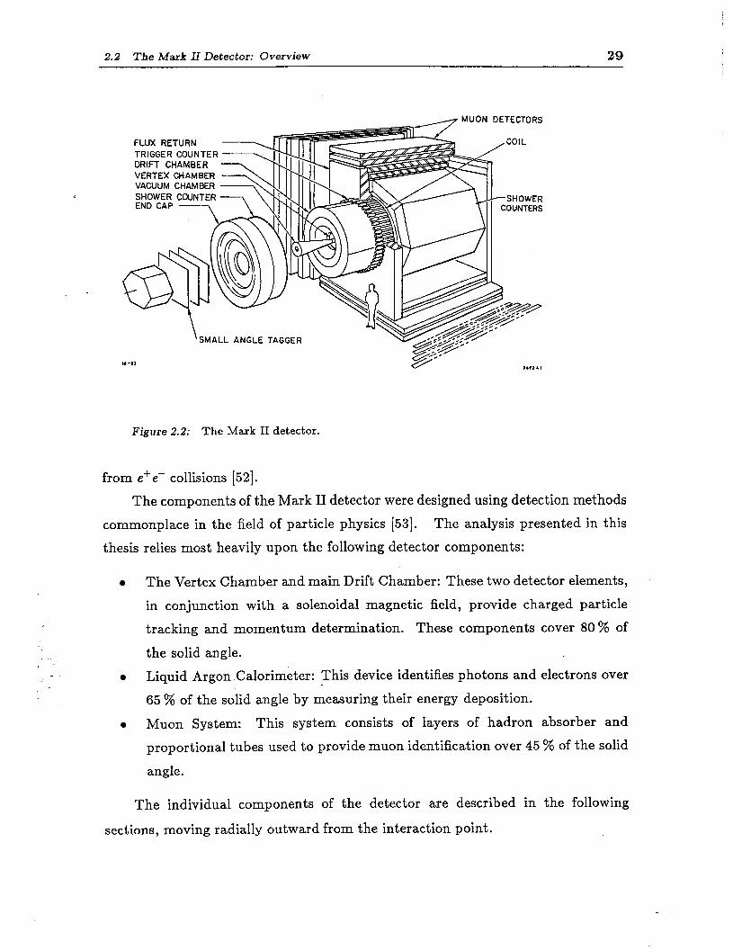
2.2 The Mark II Detector: Overview 29
w. . I . . “I .-..11+1.
VERTEX CHAMBER VACUUM CHAMBER SHOWER COUNTER %k/ibf END CAP -
7
‘SMALL ANGLE TAGGER
Figure 2.2: The Mark II detector.
from e+e- collisions [52].
The components of the Mark II detector were designed using detection methods
commonplace in the field of particle physics [53]. The analysis presented in this
thesis relies most heavily upon the following detector components:
0 The Vertex Chamber and main Drift Chamber: These two detector elements,
in conjunction with a solenoidal magnetic field, provide charged particle
tracking and momentum determination. These components cover 80 % of
the solid angle.
0 Liquid Argon Calorimeter: This device identifies photons and electrons over
65 % of the solid angle by measuring their energy deposition.
0 Muon System: This system consists of layers of hadron absorber and
proportional tubes used to provide muon identification over 45 % of the solid
angle.
The individual components of the detector are described in the following
sections, moving radially outward from the interaction point.
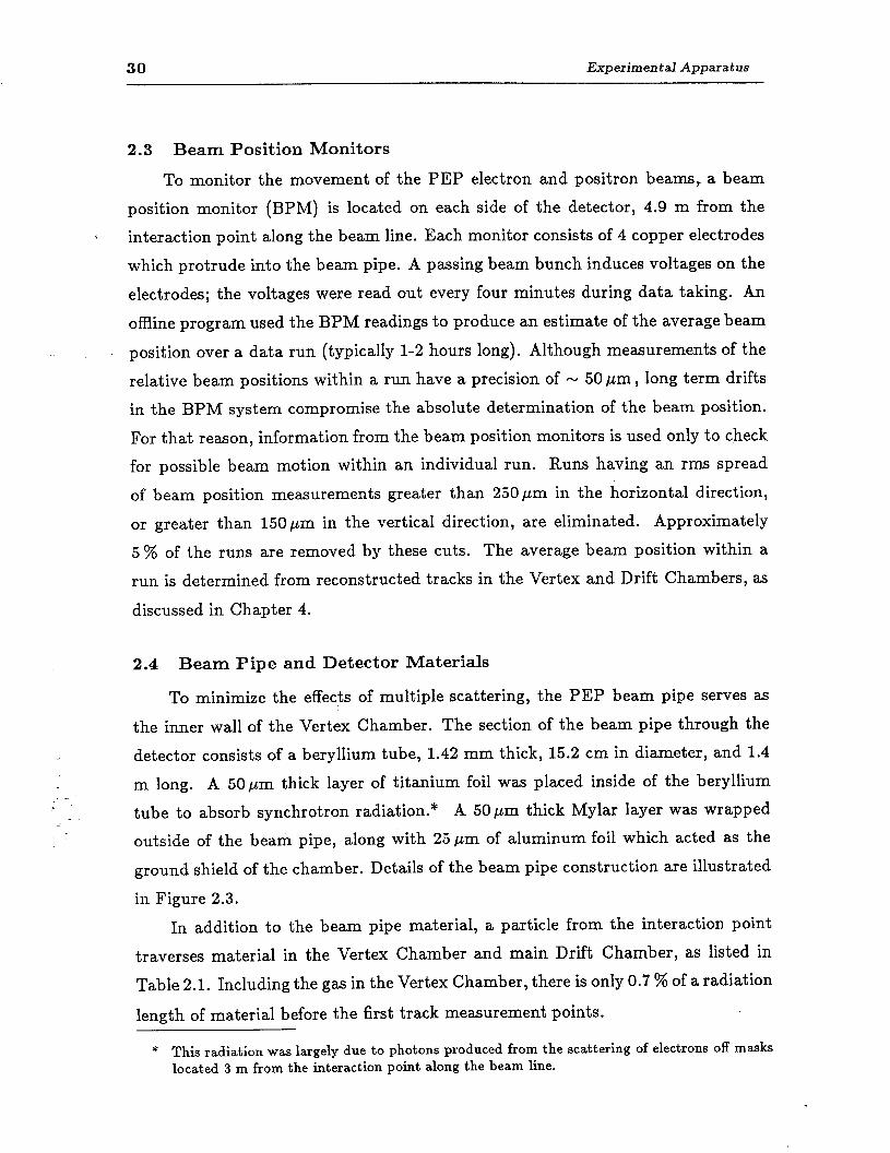
30 Experimental Apparatus
2.3 Beam Position Monitors
To monitor the movement of the PEP electron and positron beams, a beam
position monitor (BPM) is located on each side of the detector, 4.9 m from the 2 interaction point along the beam line. Each monitor consists of 4 copper electrodes
which protrude into the beam pipe. A passing beam bunch induces voltages on the
electrodes; the voltages were read out every four minutes during data taking. An
offline program used the BPM readings to produce an estimate of the average beam
- position over a data run (typically l-2 hours long). Although measurements of the
relative beam positions within a run have a precision of N 50 pm, long term drifts
in the BPM system compromise the absolute determination of the beam position.
For that reason, information from the beam position monitors is used only to check
for possible beam motion within an individual run. Runs having an rms spread
of beam position measurements greater than 250pm in the horizontal direction,
or greater than 15Opm in the vertical direction, are eliminated. Approximately
5 % of the runs are removed by these cuts. The average beam position within a
run is determined from reconstructed tracks in the Vertex and Drift Chambers, as
discussed in Chapter 4.
2.4 Beam Pipe and Detector Materials
To minimize the effects of multiple scattering, the PEP beam pipe serves as
the inner wall of the Vertex Chamber. The section of the beam pipe through the
detector consists of a beryllium tube, 1.42 mm thick, 15.2 cm in diameter, and 1.4 m long. A 5Opm thick layer of titanium foil was placed inside of the beryllium
tube to absorb synchrotron radiation. * A 50pm thick Mylar layer was wrapped
outside of the beam pipe, along with 25 pm of aluminum foil which acted as the
ground shield of the chamber. Details of the beam pipe construction are illustrated
in Figure 2.3.
In addition to the beam pipe material, a particle from the interaction point
traverses material in the Vertex Chamber and main Drift Chamber, as listed in
Table 2.1. Including the gas in the Vertex Chamber, there is only 0.7 % of a radiation
length of material before the first track measurement points.
* This radiation was largely due to photons produced from the scattering of electrons off masks located 3 m from the interaction point along the beam line.
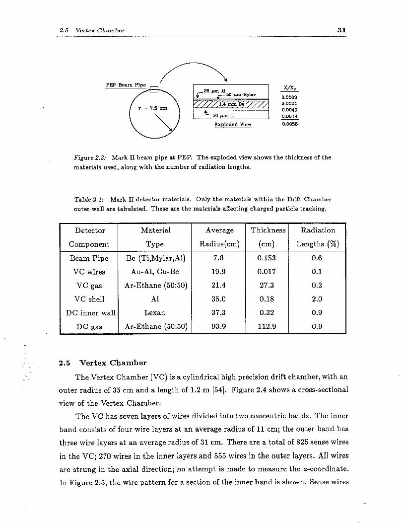
2.5 Vertex Chamber 31
r = 7.5 cm
ne -- I. ar
///// 1.k ‘%n’& ‘////
+-SOpInTs
Exploded View
0.0003 0.0001 0.0040 0.0014 0.0058
Figure 2.3: Mark II beam pipe at PEP. The exploded view shows the thickness of the materials used, along with the number of radiation lengths.
Table 2.1: Mark II detector materials. Only the materials within the Drift Chamber outer wall are tabulated. These are the materials affecting charged particle tracking.
Detector
Component
Beam Pipe
VC wires
VC gas
VC shell
DC inner wall
DC gas
Material Average
Type Radius (cm)
Be (Ti,Mylar,Al) 7.6
Au-Al, Cu-Be 19.9
Ar-Ethane (50:50) 21.4
Al 35.0
Lexan 37.3
Ar-Ethane (50:50) 93.9
Thickness Radiation
( 1 cm Lengths (%)
0.153 0.6 0.017 0.1
27.3 0.2
0.18 2.0 0.32 0.9
112.9 0.9
. -- 2.5 Vertex Chamber
The Vertex Chamber (VC) is a cylindrical high precision drift chamber, with an
outer radius of 35 cm and a length of 1.2 m [54]. Figure 2.4 shows a cross-sectional
view of the Vertex Chamber.
The VC has seven layers of wires divided into two concentric bands. The inner
band consists of four wire layers at an average radius of 11 cm; the outer band has
three wire layers at an average radius of 31 cm. There are a total of 825 sense wires
in the VC; 270 wires in the inner layers and 555 wires in the outer layers. All wires are strung in the axial direction; no attempt is made to measure the z-coordinate.
In Figure 2.5, the wire pattern for a section of the inner band is shown. Sense wires
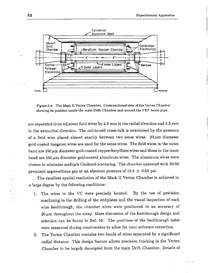
32 Experiment al Apparatus
Cylindrical / Aluminum Shell
1 Marktl Dri
/Beryllium Vacuum Chamber 1 I Electrc
10-83 n 4268446
Figure 2.4: The Mark II Vertex Chamber. Cross-sectional view of the Vertex Chamber showing its position inside the main Drift Chamber and around the PEP beam pipe.
are separated from adjacent field wires by 4.2 mm in the radial direction and 5.3 mm
in the azimuthal direction. The cell-to-cell cross-talk is minimized by the presence
of a field wire placed almost exactly between two sense wires. 2Opm diameter
gold-coated tungsten wires are used for the sense wires. The field wires in the outer
band are 150 pm diameter gold-coated copper-beryllium wires and those in the inner
band are 150 pm diameter gold-coated aluminum wires. The aluminum wires were
chosen to minimize multiple Coulomb scattering. The chamber operated with 50:5O
premixed argon-ethane gas at an absolute pressure of 15.5 31 0.05 psi.
The excellent spatial resolution of the Mark II Vertex Chamber is achieved to
-_ a large degree by the following conditions: : ._
-- - 1. The wires in the VC were precisely located. By the use of precision
machining in the drilling of the endplates and the visual inspection of each
wire feedthrough, the chamber wires were positioned to an accuracy of
20 pm throughout the array. More discussion of the feedthrough design and
selection can be found in Ref. 55. The positions of the feedthrough holes
were measured during construction to allow for later software correction.
2. The Vertex Chamber contains two bands of wires separated by a significant
radial distance. This design feature allows precision tracking in the Vertex
Chamber to be largely decoupled from the main Drift Chamber. Details of
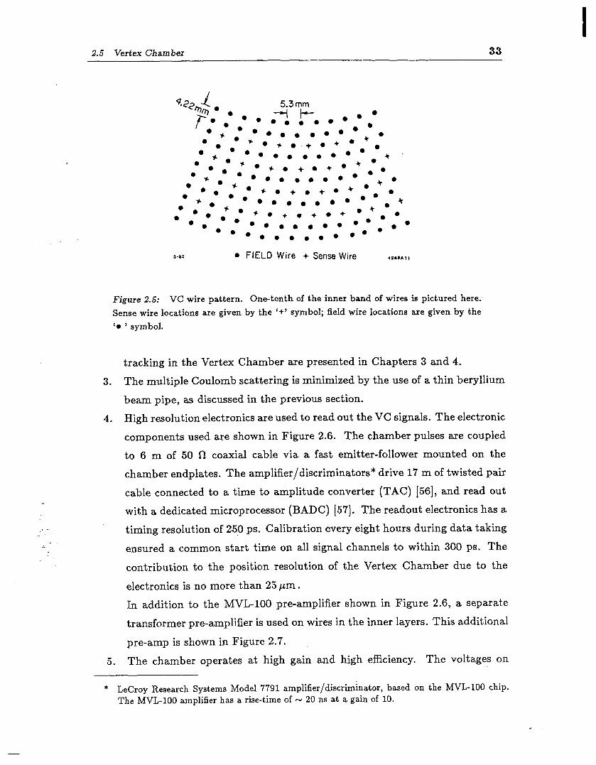
2.5 Vertex Chamber 33
:
1 0 l - * . +o+*+ l + - 9 l l
**+ l **.***
+ l t
l .*o *+a+*+’
0 b
0 **+ l **..*** do
0 l * l
-+
g+e+*+*+*** 0 l oooo**
9 +*+a+*+ 9 + l +
9 9 I .o .*o l .** l
l 9 l o***
l ***.** l o l *
l 0
l
3-82 l FIELD Wire + Sense Wire 4269A‘l
Figure 2.5: VC wire pattern. One-tenth of the inner band of wires is pictured here. Sense wire locations are given by the ‘+’ symbol; field wire locations are given by the ‘0 ’ symbol.
3.
4.
tracking in the Vertex Chamber are presented in Chapters 3 and 4.
The multiple Coulomb scattering is minimized by the use of a thin beryllium
beam pipe, as discussed in the previous section.
High resolution electronics are used to read out the VC signals. The electronic
components used are shown in Figure 2.6. The chamber pulses are coupled
to 6 m of 50 St coaxial cable via a fast emitter-follower mounted on the
chamber endplates. The amplifier/discriminators* drive 17 m of twisted pair
cable connected to a time to amplitude converter (TAC) 1561, and read out
with a dedicated microprocessor (BADC) [57]. The readout electronics has a
timing resolution of 250 ps. Calibration every eight hours during data taking
ensured a common start time on all signal channels to within 300 ps. The
contribution to the position resolution of the Vertex Chamber due to the
electronics is no more than 25 pm.
In addition to the MVL-100 pre-amplifier shown in Figure 2.6, a separate
transformer pre-amplifier is used on wires in the inner layers. This additional
pre-amp is shown in Figure 2.7.
5. The chamber operates at high gain and high efficiency. The voltages on
* LeCroy Research Systems Model 7791 amplifier/discriminator, based on the MVL-100 chip. The MVL-100 amplifier has a rise-time of N 20 ns at a gain of 10.
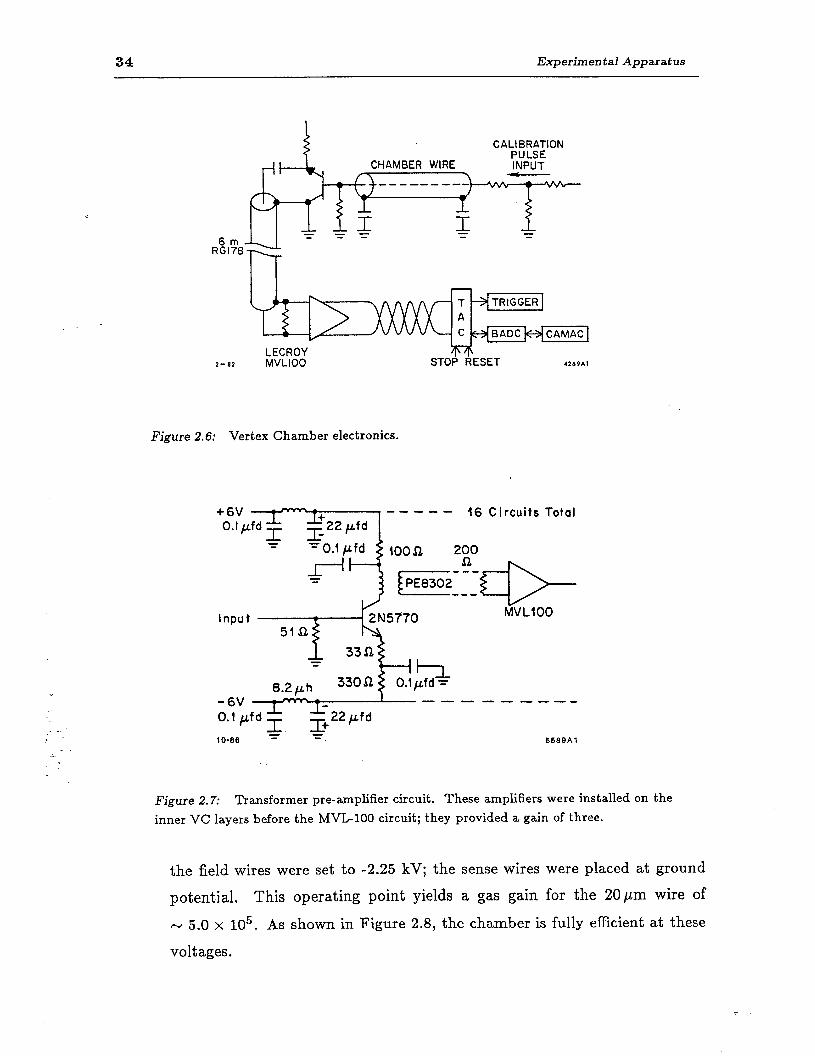
34 Experimental Apparatus
I CALI BRATION
CAMAC
426911
Figure 2.6; Vertex Chamber electronics.
+6 0.
m---w 16 Circuits Total
Input MC100
-6V I v-------w 0.1 tL’d $ ?+22pfd
lo-86 = = 6589Al
Figure 2.7: ntansformer pre-amplifier circuit. These amplifiers were installed on the
inner VC layers before the MVL-100 circuit; they provided a gain of three.
the field wires were set to -2.25 kV; the sense wires were placed at ground
potential. This operating point yields a gas gain for the 2Qm wire of
- 5.0 x 10⁵. As shown in Figure 2.8, the chamber is fully efficient at these
voltages.
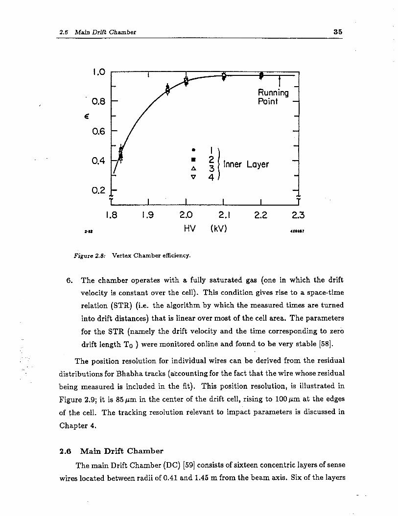
2.6 Main Drift Chamber 35
0.8 e
0.6
I
i-02
1 T
t
Running Point
-
-
-
v 4 I Inner Layer -
-
* I I
.8 I .9 2.0 2.1 2.2 2.3 HV (kV) 426987
Figure 2.8: Vertex Chamber efficiency.
6. The chamber operates with a fully saturated gas (one in which the drift
velocity is constant over the cell). This condition gives rise to a space-time
relation (STR) ( i.e. the algorithm by which the measured times are turned
into drift distances) that is linear over most of the cell area. The parameters
for the STR (namely the drift velocity and the time corresponding to zero
drift length To ) were monitored online and found to be very stable [58].
The position resolution for individual wires can be derived from the residual
distributions for Bhabha tracks (accounting for the fact that the wire whose residual
being measured is included in the fit). This position resolution, is illustrated in
Figure 2.9; it is 85pm in the center of the drift cell, rising to 100pm at the edges
of the cell. The tracking resolution relevant to impact parameters is discussed in
Chapter 4.
2.6 Main Drift Chamber
The main Drift Chamber (DC) [59] consists of sixteen concentric layers of sense
wires located between radii of 0.41 and 1.45 m from the beam axis. Six of the layers
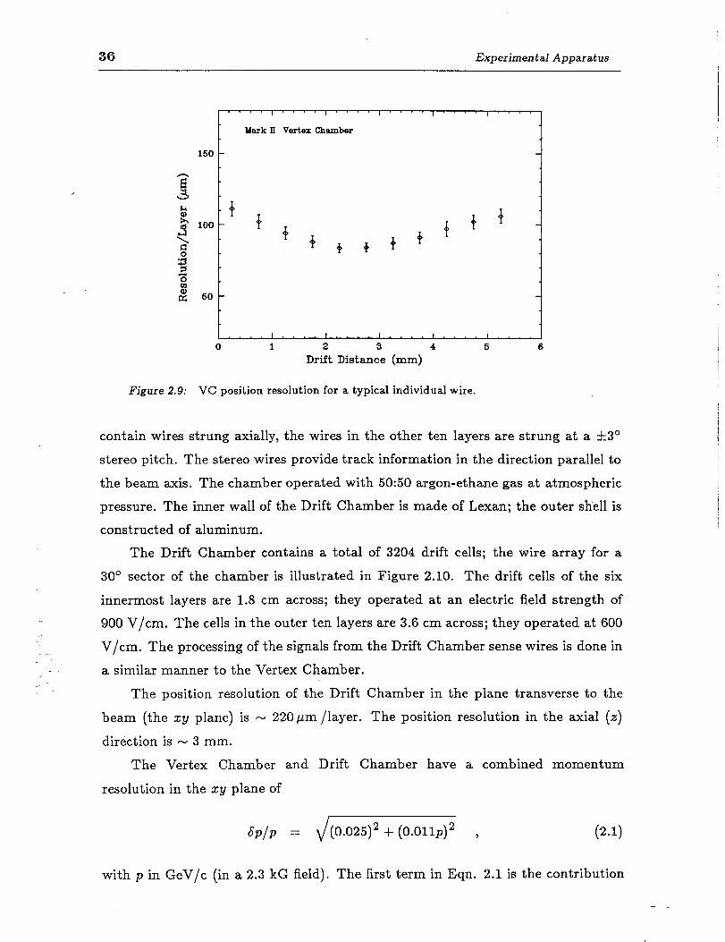
36 Experimental Apparatus
0 1 2 3 4 5 6 Drift. Distance (mm)
Figure 2.9: VC position resolution for a typical individual wire.
contain wires strung axially, the wires in the other ten layers are strung at a ~t3O
stereo pitch. The stereo wires provide track information in the direction parallel to
the beam axis. The chamber operated with 50:50 argon-ethane gas at atmospheric
pressure. The inner wall of the Drift Chamber is made of Lexan; the outer shell is
constructed of aluminum.
The Drift Chamber contains a total of 3204 drift cells; the wire array for a
30° sector of the chamber is illustrated in Figure 2.10. The drift cells of the six
innermost layers are 1.8 cm across; they operated at an electric field strength of
900 V/cm. The cells in the outer ten layers are 3.6 cm across; they operated at 600
_ _ i V/cm. The processing of the signals from the Drift Chamber sense wires is done in
a similar manner to the Vertex Chamber.
The position resolution of the Drift Chamber in the plane transverse to the
beam (the zy plane) is - 220 pm /layer. The position resolution in the axial (z)
direction is - 3 mm.
The Vertex Chamber and Drift Chamber have a combined momentum
resolution in the zy plane of
&PIP = J (0.025)2 + (0.011~)~ , c24
with p in GeV/c ( in a 2.3 kG field). The first term in Eqn. 2.1 is the contribution
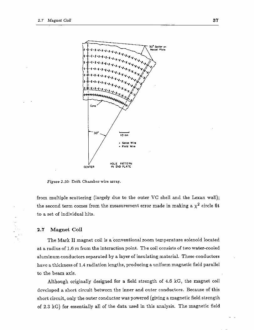
2.7 Magnet Coil 37
CE
0 !&rise Wire l Field Wire
HOLE PATTERN INTER IN END PLATE
Figure 2.10: Drift Chamber wire array.
from multiple scattering (largely due to the outer VC shell and the Lexan wall);
the second term comes from the measurement error made in making a x2 circle fit
to a set of individual hits.
2.7 Magnet Coil
The Mark II magnet coil is a conventional room temperature solenoid located
at a radius of 1.6 m from the interaction point. The coil consists of two water-cooled
aluminum conductors separated by a layer of insulating material. These conductors
have a thickness of 1.4 radiation lengths, producing a uniform magnetic field parallel
to the beam axis.
Although originally designed for a field strength of 4.6 kG, the magnet coil
developed a short circuit between the inner and outer conductors. Because of this
short circuit, only the outer conductor was powered (giving a magnetic field strength
of 2.3 kG) for essentially all of the data used in this analysis. The magnetic field
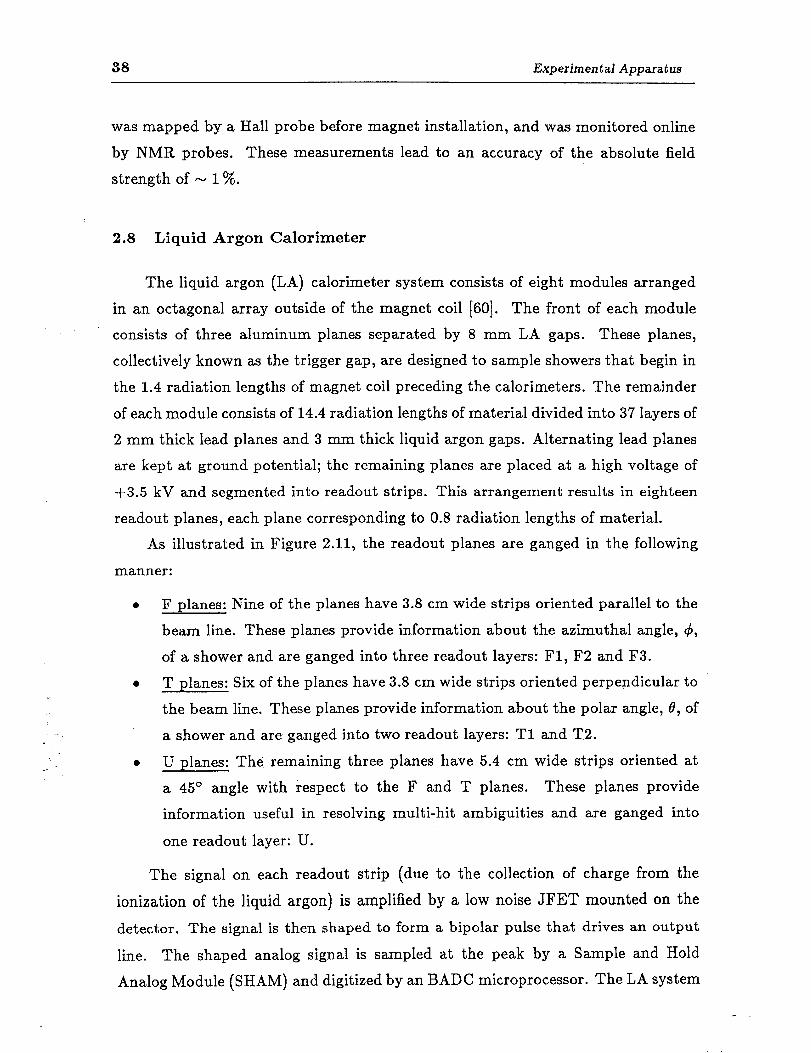
38 Experimental Apparatus
was mapped by a Hall probe before magnet installation, and was monitored online
by NMR probes. These measurements lead to an accuracy of the absolute field
strength of - 1%.
c
2.8 Liquid Argon Calorimeter
The liquid argon (LA) calorimeter system consists of eight modules arranged
in an octagonal array outside of the magnet coil [60]. The front of each module - consists of three aluminum planes separated by 8 mm LA gaps. These planes,
collectively known as the trigger gap, are designed to sample showers that begin in
the 1.4 radiation lengths of magnet coil preceding the calorimeters. The remainder
of each module consists of 14.4 radiation lengths of material divided into 37 layers of
2 mm thick lead planes and 3 mm thick liquid argon gaps. Alternating lead planes
are kept at ground potential; the remaining planes are placed at a high voltage of
+3.5 kV and segmented into readout strips. This arrangement results in eighteen
readout planes, each plane corresponding to 0.8 radiation lengths of material.
As illustrated in
manner:
0 F planes: Nine
Figure 2.11, the readout planes are ganged in the following
of the planes have 3.8 cm wide strips oriented parallel to the
beam line. These planes provide information about the azimuthal angle, 4,
of a shower and are ganged into three readout layers: Fl, F2 and F3.
T planes: Six of the planes have 3.8 cm wide strips oriented perpendicular to
the beam line. These planes provide information about the polar angle, 8, of
a shower and are ganged into two readout layers: Tl and T2.
U planes: The remaining three planes have 5.4 cm wide strips oriented at
a 45O angle with respect to the F and T planes. These planes provide
information useful in resolving multi-hit ambiguities and are ganged into
one readout layer: U.
The signal on each readout strip (due to the collection of charge from the
ionization of the liquid argon) is amplified by a low noise JFET mounted on the detector. The signal is then shaped to form a bipolar pulse that drives an output
line. The shaped analog signal is sampled at the peak by a Sample and Hold
Analog Module (SHAM) and digitized by an BADC microprocessor. The LA system
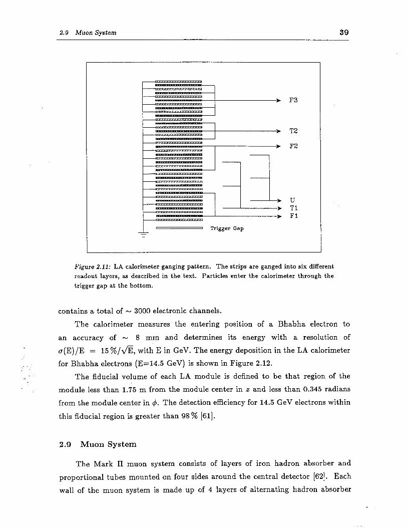
2.9 Muon System 39
Trigger Gap
F3
T2
F2
U Tl Fl
Figure 2.11: LA calorimeter ganging pattern. The strips are ganged into six different readout layers, as described in the text. Particles enter the calorimeter through the trigger gap at the bottom.
contains a total of - 3000 electronic channels.
The calorimeter measures the entering position of a Bhabha electron to
an accuracy of - 8 mm and determines its energy with a resolution of
cr(E)/E = 15 %/a, with E in GeV. The energy deposition in the LA calorimeter
for Bhabha electrons (E=l4.5 GeV) is shown in Figure 2.12.
The fiducial volume of each LA module is defined to be that region of the
module less than 1.75 m from the module center in z and less than 0.345 radians
from the module center in 4. The detection efficiency for 14.5 GeV electrons within
this fiducial region is greater than 98 % [61].
2.9 Muon System
The Mark II muon system consists of layers of iron hadron absorber and
proportional tubes mounted on four sides around the central detector [62]. Each
wall of the muon system is made up of 4 layers of alternating hadron absorber
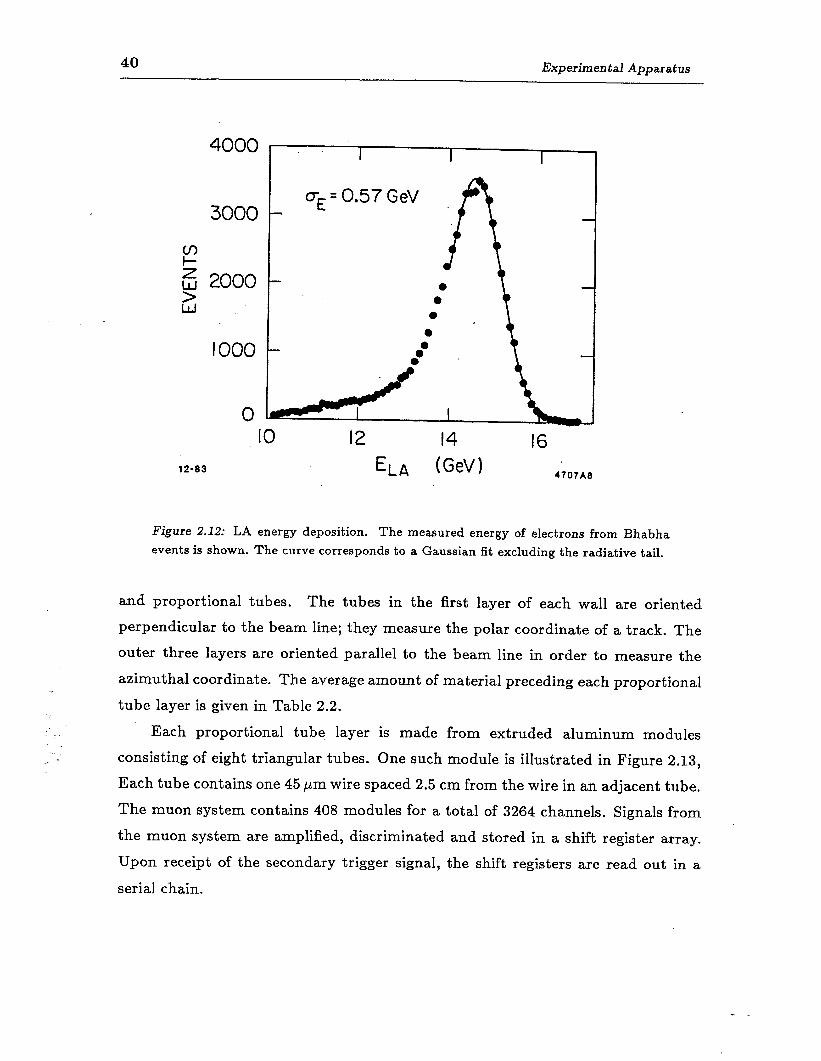
40 Experimental Apparatus
IO00
12-83 EL, (GeV) 16
41DfA0
Figure 2.12: LA energy deposition. The measured energy of electrons from Bhabha events is shown. The curve corresponds to a Gaussian fit excluding the radiative tail.
and proportional tubes. The tubes in the first layer of each wall are oriented perpendicular to the beam line; they measure the polar coordinate of a track. The
outer three layers are oriented parallel to the beam line in order to measure the
azimuthal coordinate. The average amount of material preceding each proportional
tube layer is given in Table 2.2.
Each proportional tube layer is made from extruded aluminum modules
consisting of eight trianguIar tubes. One such module is illustrated in Figure 2.13,
Each tube contains one 45 pm wire spaced 2.5 cm from the wire in an adjacent tube.
The muon system contains 408 modules for a total of 3264 channels. Signals from
the muon system are amplified, discriminated and stored in a shift register array.
Upon receipt of the secondary trigger signal, the shift registers are read out in a
serial chain.
2.10 Other Systems 41
Table 2.2: Hadron absorber thickness. The number of interaction lengths is given (averaged over the four muon walls) for a hadron at normal incidence.
Layer Layer Coil and LA Coil and LA
1 1
2 2
3 3
4 4
Interaction Lengths
1.2
2.6
4.0
5.8
7.4
4 20 cm b
, < Y 2.5 cm
Figure 2.13: Muon system cross-sectional view. A single module is shown.
2.10 Other Systems
Several components of the Mark II detector are not directly used in this
analysis. For completeness, they are briefly described here.
2.10.1 Time of Aiglzt system _
The Time of Flight (TOF) system is positioned on the outside of the Drift
Chamber and inside the magnet coil. This system consists of 48 plastic scintillation
counters at a radius of 1.51 m; it covers 75 % of the solid angle. Each counter (1
in thick Pilot F scintillator) runs parallel to the beam direction and is viewed at
each end by a photomultiplier tube. The rms timing resolution is - 350 ps. The
TOF system provides r/K separation up to a momentum of 1 GeV/c and proton identification up to 2 GeV/c. The TOF system is used in the event trigger and to
reject cosmic ray events.
42 Experimental Apparatus
2.10.2 Endcap calorimeters
The endcap calorimeters are positioned at each end of the detector, covering
polar angles between l5O and 40° . These calorimeters consist of 2.3 radiation
lengths of lead followed by two layers of proportional chambers; they achieve an
energy resolution of a(E)/E = 50%/&Z (E in GeV) for photons and electrons.
2.10.3 Small angle tagging system
The small angle tagging (SAT) system provides charged particle tracking and
calorimetry in the region on each side of the detector at low angles ( 20 to 80 mr)
from the beam line. The SAT system is used to detect electrons from small angle
Bhabha scattering events or from two-photon interactions. From the rate of small
angle Bhabha events the luminosity is determined to 9~5 % accuracy.
2.11 Event Trigger System
The time between beam crossings at PEP is quite short (2.4 ps); therefore a
trigger system is needed to control the selective recording of data onto magnetic
tape. The Mark II trigger system is composed of two levels: a fast primary trigger
designed to work between beam crossings and a slower (intelligent) hardware track-
finder [63].
The primary logic demands that any one of the following conditions be met in
coincidence with a beam crossing signal:
Primary Trigger Conditions
1. Charged trigger: There must be hits in at least nine layers of the VC and DC
systems and in at least one-TOF counter.
2. Neutral trigger: The summed energy deposition in the front half of the eight
LA modules and in the endcap modules must be greater than 4 GeV or
there must be at least 1 GeV of energy deposited in the front half of two LA
modules.
3. Bhabha trigger: The SAT system must signal the presence of a collinear
e’e- event. This trigger is prescaled by a factor of 16 to reduce its rate.
The primary trigger determination takes - 1 ps to complete, resulting in no
system deadtime.
2.12 Operating Conditions 43
If the primary trigger logic is satisfied, data collection halts and secondary
trigger processing begins. A hardware track processor searches for charged tracks
employing the information from the VC, DC and TOF systems. These tracks (called
hardware tracks) are identified by programmed curvature modules which search for
track candidates by requiring a certain number of hits along an arc extending from
the interaction point.
The secondary trigger logic requires that any one of the following conditions
be met:
Secondary Trigger Conditions
1. Charged trigger: There must be at least two hardware tracks; each track must
have momentum greater than 100 MeV/ c and must lie within the central 65 %
of the detector.
2. Neutral trigger: The same conditions as in the neutral primary trigger must
be met, or there must be one hardware track found and one LA module found
with energy deposition in the front half greater than 1 GeV.
3. Bhabha Trigger: Every one out of sixteen Bhabha primary triggers.
The secondary trigger determination takes 33 ps to complete. At a typical
primary trigger rate of 1 kHz, the secondary trigger processing results in a deadtime
of N 3 %. Typical secondary trigger rates were l-2 Hz.
2.12 Operating Conditions
The Mark II experiment accumulated a total of 206 pb-’ of data in three years
of ,operation at PEP. During this time, a number of detector systems experienced
hardware problems. Because of the importance of the charged particle tracking on
the analysis presented in this thesis, only the problems associated with the Drift
Chamber and Vertex Chamber are discussed here.
2.12.1 Drift Chamber operation
In the fall of 1982, the Drift Chamber experienced problems associated with
high voltage discharge. These problems necessitated a lowering of the operating
voltages in the chamber for a time; the lower voltages resulted in a reduction of 10 %
in the overall tracking efficiency. Approximately 25 pb-’ of data were accumulated
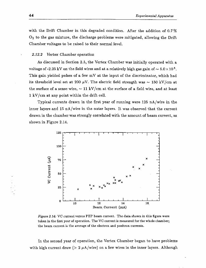
44 Experimental Apparatus
with the Drift Chamber in this degraded condition. After the addition of 0.7%
02 to the gas mixture, the discharge problems were mitigated, allowing the Drift
Chamber voltages to be raised to their normal level.
c 2.12.2 Vertex Chamber operation
As discussed in Section 2.5, the Vertex Chamber was initially operated with a
voltage of -2.25 kV on the field wires and at a relatively high gas gain of - 5.0 x 10 5.
This gain yielded pulses of a few mV at the input of the discriminator, which had
- its threshold level set at 200 JLV. The electric field strength was - 150 kV/cm at
the surface of a sense wire, - 11 kV/cm at the surface of a field wire, and at least
1 kV/cm at any point within the drift cell.
Typical currents drawn in the first year of running were 125 nA/wire in the
inner layers and 15 nA/wire in the outer layers. It was observed that the current
drawn in the chamber was strongly correlated with the amount of beam current, as
shown in Figure 2.14.
12511 1 IIll 1 II I II I I I I, I I
100 -
h
3
75 - X
2 #
#
E #
8 50v # xx
s x *x xx xx 25 - xX x%
X X X
0 ” ” ” ” ” ” ” ” ” ” 10 12 14 16,
Beam Current (mA)
Figure 2.14: VC current versus PEP beam current. The data shown in this figure were taken in the first year of operation. The VC current is measured for the whole chamber; the beam current is the average of the electron and positron currents.
In the second year of operation, the Vertex Chamber began to have problems
with high current draw (> 2 PA/wire) on a few wires in the inner layers. Although
2.12 Operating Conditions 45
the high voltage on several wires was removed, it became difficult to operate one-fifth
of the inner band of wires because of high voltage trips. The voltages on the field
wires in this section were lowered to 1.95 kV and those on the wires in the remaining
four-fifths of the inner band were lowered to 2.1 kV. At the suggestion of Atac [64], c
the chamber gas was bubbled through ethanol at O” C, giving 1.5 % ethanol by
volume. W ith these operating conditions, wires in the inner layers typically drew
80 nA of current each and the chamber was stable.
2.12.3 Test chamber study
In order to reproduce the symptoms of chamber aging seen in the VC, a small
test chamber was constructed. This test chamber contained twelve complete drift
cells with the same cell geometry and types of wire as in the inner band of the
VC. The test chamber was operated with -2.25 kV on the field wires and with
50:5O argon-ethane gas (no ethanol). A 4.3 mCi Co60 source was used to bombard
the chamber with radiation; this source induced - 500 nA/wire of current. The
test chamber began to show serious degradation after approximately 0.08 C/cm of
charge had been collected on each wire. Once degradation was evident, a smaller
1.5 mCi Co60 source was used to irradiate the chamber.*
The degradation in the test chamber was characterized by symptoms quite
_- _ __
similar to those observed in the VC. The test chamber drew large currents or
suffered high voltage breakdown at the designated operating point. Reducing the
high voltage lowered these currents until a threshold voltage (1.8 kV) was reached,
below which the current was close to normal. By raising the high voltage again, the
breakdown conditions could be re-estab1ished.t This behavior was consistent with
the deposition of polymer layers on wires observed by other experimenters [65]. This
layer acts as an insulator (capacitor) and allows the build-up of charge on its surface
to the point where breakdown can occur. In order to determine if the breakdown
behavior observed in the test chamber was consistent with the presence of a layer
* The large source was used to produce degradation in the chamber in a reasonable amount of time, while the smaller source was used to study the symptoms of the degradation after it occured. This latter source was positioned so that the amount of current drawn per wire by the test chamber was the same as that drawn by the VC in the PEP beam.
t At first, it seemed as if the threshold voltage to re-establish breakdown conditions was higher than the voltage where breakdown disappeared, i.e. that a hysteresis behavior was being observed. This hysteresis behavoir was eliminated, however, by waiting at each point while raising the high voltage.
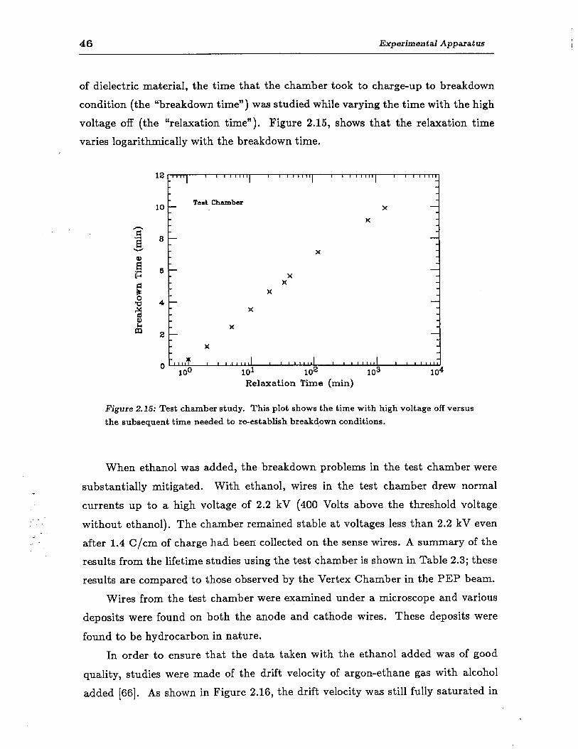
46 Experimental Apparatus
of dielectric material, the time that the chamber took to charge-up to breakdown
condition (the “breakdown time”) was studied while varying the time with the high
voltage off (the “relaxation time”). Figure 2.15, shows that the relaxation time
varies logarithmically with the breakdown time.
12 I I II’] I I I lllll I I111111~ I I Illlll, I I Illl-m
10 -
B-
6-
4-
2-
Text Chamber
x #
#
#
# X
X
0 t--IT ’ I I wlJ I I I111111 I I I1111l1 I I IIIIlLj
100 101 102 103 104 Relaxation Time (min)
Figure 2.15: Test chamber study. This plot shows the time with high voltage off versus the subsequent time needed to re-establish breakqown conditions.
When ethanol was added, the breakdown problems in the test chamber were
substantially mitigated. With ethanol, wires in the test chamber drew normal
currents up to a high voltage of 2.2 kV (400 Volts above the threshold voltage
without ethanol). The chamber remained stable at voltages less than 2.2 kV even
after 1.4 C/cm of charge had been collected on the sense wires. A summary of the
results from the lifetime studies using the test chamber is shown in Table 2.3; these
results are compared to those observed by the Vertex Chamber in the PEP beam.
Wires from the test chamber were examined under a microscope and various
deposits were found on both the anode and cathode wires. These deposits were
found to be hydrocarbon in nature.
In order to ensure that the data taken with the ethanol added was of good
quality, studies were made of the drift velocity of argon-ethane gas with alcohol
added [66]. As shown in Figure 2.16, the drift velocity was still fully saturated in

2.12 Operating Conditions 47
Table 2.3: Chamber lifetime study. Q1 is the charge integrated on sense wires before degradation occured; Q2 is the charge integrated after the addition of ethanol. VI is the breakdown voltage, above which the chamber drew unacceptable current without ethanol; V2 is the same quantity with ethanol. The integrated charge for the Vertex Chamber was estimated by assuming that all the charge was collected in the central 50
cm of the chamber.
Quantity
Ql (C/cm)
92 (C/cm)
J5 (W
v2 (kV)
Test Chamber I Vertex Chamber
0.08 0.03
> 1.3 > 0.14
1.80 1.75
2.20 NA
four-fifths of the inner band of wires in the VC after the addition of ethanol. In the
remaining one-fifth of the inner band, the drift velocity was saturated over most of
the drift cell.
80 -
0 O 53 8 6 8 8 g n i! 0 #
B # 3 40- 0
3 *r-l :: #
2 20 - ti 0 Ar-Ethane (60:60)
g # X Ar-Ethane (50:50)+15X Ethanol _
0 ! I I I I I I I I I I 1 I I I I 0 0.5 1 1.5 2
Electric Field Strength (kV/cm)
Figure 2.16: Drift velocity with and without ethanol added to VC gas, The Vertex Chamber operated at typical field strengths of - 1.1 kV/cm (no lower than 0.9 kV/cm) for four-fifths of the inner band of wires. In the remaining one-fifth of the inner band, the field strengths were typically 0.9 kV/cm (no lower than 0.7 kV/cm).
The tracking efficiency of the Vertex Chamber with ethanol added was checked,
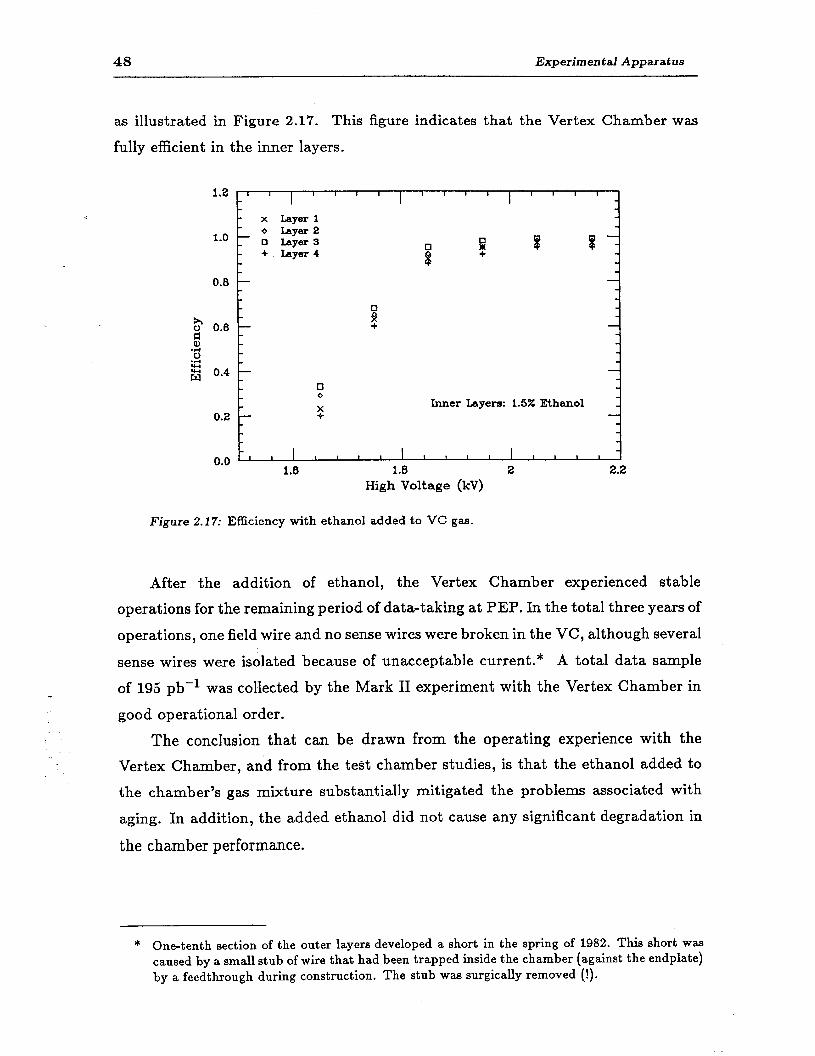
48 Experimental Apparatus
as illustrated in Figure 2.17. This figure indicates that the Vertex Chamber was
fully efficient in the inner layers.
q h 9
z OS6 +
- Q) *PI 0
G g 0.4 -
q 0
Inner Layers: 1.5% Ethanol 0.2 - :
lb2 II 1 IIll 1 I III 1 Ill I.
- x Layer 1 -
1.0 0
Layer 2
- _ 0 Layer 3
- + Layer 4
0 B B $
8:
0.8 -
0.0 ” ” ” ” ” ” I”” - 1.6 1.8 2 2.2
High Voltage (kV)
Figure 2.17: Efficiency with ethanol added to VC gas.
After the addition of ethanol, the Vertex Chamber experienced stable
operations for the remaining period of data-taking at PEP. In the total three years of
operations, one field wire and no sense wires were broken in the VC, although several
sense wires were isolated because of unacceptable current.* A total data sample
of 195 pb-l was collected by the Mark II experiment with the Vertex Chamber in
good operational order.
The conclusion that can be drawn from the operating experience with the
Vertex Chamber, and from the test chamber studies, is that the ethanol added to
the chamber’s gas mixture substantially mitigated the problems associated with
aging. In addition, the added ethanol did not cause any significant degradation in
the chamber performance.
* One-tenth section of the outer layers developed a short in the spring of 1982. This short was caused by a small stub of wire that had been trapped inside the chamber (against the endplate) by a feedthrough during construction. The stub was surgically removed (!).
Chapter 3
Event Reconstruction and Simulation
Before it can be used for physics analysis, the raw data taken by the experiment
must be processed and manipulated into a more readily understood form. This
processing, or event reconstruction, involves charged particle tracking and particle
identification.
In this chapter, the basic procedure by which charged tracks are found in the
Vertex Chamber and Drift Chamber is discussed. A discussion of the improvements
to this basic procedure to achieve the optimum position resolution is postponed until
Chapter 4. Charged tracks are extrapolated from the Drift Chamber into the LA
calorimeter and muon system in order to identify electrons and muons, respectively.
The procedures for lepton identification are outlined in Chapter 5; these procedures
constitute the only use of particle identification in this thesis.
In addition to digesting data taken by the detector, the event reconstruction
package is used to process events generated by Monte Carlo programs. These
programs simulate the relevant physics for the production of final state particles
from e+e- collisions, as well as the detector response to the final state particles.
The Mark II Monte Carlo simulation is outlined in the latter half of this chapter;
the optimization of the Monte Carlo is discussed. This discussion outlines the basic
properties of C and B hadron production and decay not covered in Chapter 1.
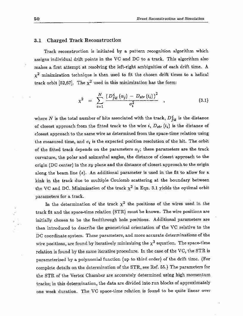
50 Event Reconstruction and Simulation
3.1 Charged Track Reconstruction
Track reconstruction is initiated by a pattern recognition algorithm which
assigns individual drift points in the VC and DC to a track. This algorithm also
makes a first attempt at resolving the left-right ambiguities of each drift time. A
x2 minimization technique is then used to fit the chosen drift times to a helical
track orbit [52,67]. The x2 used in this minimization has the form:
x2 = N ( Diit (Qj) - Dstr (t;) )2 c ai; 3
i=l (3 1) .
where N is the total number of hits associated with the track, Dji, is the distance
of closest approach from the fitted track to the wire i, Dstr (ti) is the distance of
closest approach to the same wire as determined from the space-time relation using
the measured time, and a; is the expected position resolution of the hit. The orbit
of the fitted track depends on the parameters aj; these parameters are the track
curvature, the polar and azimuthal angles, the distance of closest approach to the
origin (DC center) in the a;y plane and the distance of closest approach to the origin
along the beam line (z). An additional parameter is used in the fit to allow for a
kink in the track due to multiple Coulomb scattering at the boundary between
the VC and DC. Minimization of the track x2 in Eqn. 3.1 yields the optimal orbit
parameters for a track.
In the determination of the track x2 the positions of the wires used in the
track fit and the space-time relation (STR) must be known. The wire positions are .- initially chosen to be the feedthrough hole positions. Additional parameters are
then introduced to describe the geometrical orientation of the VC relative to the
DC coordinate system. These parameters, and more accurate determinations of the
wire positions, are found by iteratively minimizing the x2 equation. The space-time
relation is found by the same iterative procedure. In the case of the VC, the STR is
parameterized by a polynomial function (up to third order) of the drift time. (For
complete details on the determination of the STR, see Ref. 55.) The parameters for
the STR of the Vertex Chamber are accurately determined using high momentum
tracks; in this determination, the data are divided into run blocks of approximately
one week duration. The VC space-time relation is found to be quite linear over
3.2 Monte Carlo Simulation 51
most of the drift cell. As discussed in Section 2.5, this linearity is due to operating
the chamber with a fully saturated gas. The x2 minimization procedure is also used
to determine the dependence of the expected resolution (i.e. ai in Eqn. 3.1) on drift
distance. As illustrated in Figure 2.9, the VC resolution is nearly flat as a function <
of drift distance.
Tracks are reconstructed by the procedure described above with high efficiency
(> 98 % for isolated tracks) over 75 % of the solid angle. Bhabha tracks are used
to determine the momentum resolution of the VC and DC systems in the 2.3 kG
magnetic field, yielding the expression given in Eqn. 2.1. The momentum resolution
is improved by 15 % by constraining tracks to pass through the interaction point.*
3.2 Monte Carlo Simulation
A detailed set of Monte Carlo programs are used to simulate events in the Mark
II detector. These routines can be divided into two sections: the hadronic event
generator and the routines subsequently used to trace particles and their decay
products through the detector.
In this analysis, the event generator used is that incorporated in the LUND
model [68], JETSET version 6.3. The event generator initially produces partons
(quarks and gluons) resulting from the electron-positron collision using a second
order matrix element calculation. Although two parton (#j) states are the most
common, the event generator also produces three (@g) and four (~q~if, @gg) parton
states. The relative production of two, three and four parton states is determined
by the strong interaction coupling constant cys, and by a parameter ymi,. This
latter parameter is the minimum scaled invariant mass two partons must have to
prevent them from being combined into one. As discussed in Chapter 1, hadrons
are produced from the partons by the process of fragmentation. In this analysis,
light quarks (u, d and s) are fragmented according to the LUND string scheme [69].
Heavy quarks (c and b) are fragmented using the Peterson formula. The values used
for some of the more important parameters of the Monte-Carlo event generator are
given in Table 3.1.
Except for the heavy quark fragmentation function parameters (i.e. Ed and ~b),
* This type of constraint is not done in this analysis because we are interested here in the decay of particles giving tracks with finite impact parameters.
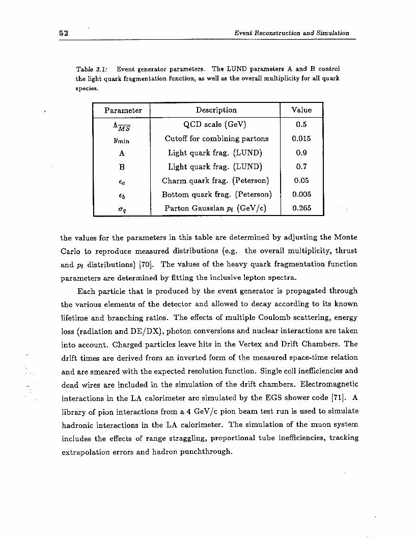
52 Event Reconstruction and Simulation
Table 3.1: Event generator parameters. The LUND parameters A and B control the light quark fragmentation function, as well as the overall multiplicity for all quark species.
Parameter
A- MS Ymin
A
B
EC
Eb
9
Description Value
QCD scale (GeV) 0.5
Cutoff for combining partons 0.015
Light quark frag. (LUND) 0.9
Light quark frag. (LUND) 0.7
Charm quark frag. (Peterson) 0.05
Bottom quark frag. (Peterson) 0.005
Parton Gaussian pt (GeV/c) 0.265
the values for the parameters in this table are determined by adjusting the Monte
Carlo to reproduce measured distributions (e.g. the overall multiplicity, thrust
and pt distributions) [70]. Th e values of the heavy quark fragmentation function
parameters are determined by fitting the inclusive lepton spectra.
Each particle that is produced by the event generator is propagated through
the various elements of the detector and allowed to decay according to its known
lifetime and branching ratios. The effects of multiple Coulomb scattering, energy
loss (radiation and DE/DX), photon conversions and nuclear interactions are taken
into account. Charged particles leave hits in the Vertex and Drift Chambers. The
drift times are derived from an inverted form of the measured space-time relation
and are smeared with the expected resolution function. Single cell inefficiencies and
dead wires are included in the simulation of the drift chambers. Electromagnetic
interactions in the LA calorimeter are simulated by the EGS shower code [71]. A
library of pion interactions from a 4 GeV/c pion beam test run is used to simulate
hadronic interactions in the LA calorimeter. The simulation of the muon system
includes the effects of range straggling, proportional tube inefficiencies, tracking
extrapolation errors and hadron punchthrough.
3.3 Optimization of the Monte Carlo 53
3.3 Optimization of the Monte Carlo
In order to ensure that the Monte Carlo simulation is reasonably correct,
it is important to compare results of the simulation to measured data. For the c time being, we limit this comparison to showing that the Monte Carlo accurately
reproduces some general distributions. The comparison of the detector simulation
to the data is considered later.*
3.3.1 Charged particle multiplicity
The charged particle multiplicity in hadronic events from e+e- collisions at
29 GeV/c has been measured by the Mark II detector at PEP [72]. The Monte
Carlo parameters are tuned to reproduce the results of this measurement, as well
as results from other experiments. In this thesis, the multiplicity of heavy quark
events is of greater interest than multiplicity averaged over all quark species. A well
identified lepton of momentum greater than 2 GeV/c signals the presence of heavy
quark decay. In Figure 3.1, the charged particle multiplicity distribution observed
in the data for such events is compared to the distribution generated by the Monte
Carlo. The data and simulation agree, indicating that the overall multiplicity in
heavy quark events is well understood. In a separate analysis of Mark II data, the
charged particle multiplicities for charm and bottom events have been measured to
be 13.2 h 0.5 5 0.9 and 16.2 & 0.5 & 1.0, respectively [73].
3.3.2 Event thrust
The jet-like structure of hadronic events from e+e- interactions was first
observed in the SLAC-LBL magnetic detector at center of mass energies of 6.2
and 7.4 GeV [74]. R esults from experiments at higher center of mass energies show
even more pronounced jet-like behavior [75]. This behavior can be understood in
terms of fragmentation of the partons produced from the e+e- collision into hadrons
with limited transverse momentum relative to the original parton direction [76].
The parameters sphericity and thrust have been introduced to quantify the two-jet
* In this analysis, great importance is placed on the detector’s ability for precision charged particle tracking and lepton identification. These topics are considered in Chapters 4 and 5, respectively.
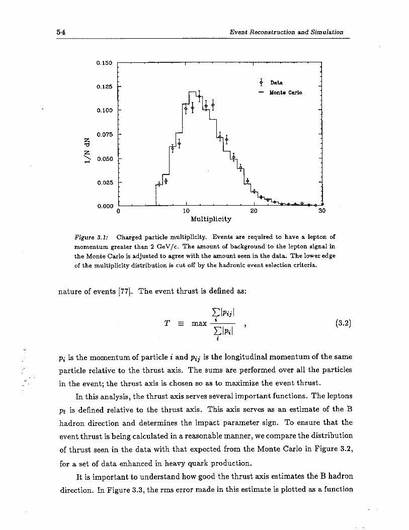
54 Event Reconstruction and Simulation
0.150 I I I
0 Data 0.125 -
0.100 -
0.075 -
53
5 0.050 -
0.025 -
0.000 10
Multiplicity
Figure 3.1: Charged particle multiplicity. Events are required to have a lepton of momentum greater than 2 GeV/c. The amount of background to the lepton signal in the Monte Carlo is adjusted to agree with the amount seen in the data. The lower edge of the multiplicity distribution is cut off by the hadronic event selection criteria.
nature of events [77]. Th e event thrust is defined as:
Cbijl T _ max ’ =
IgPiI ’ (3 2) .
pi is the momentum of particle i and p;j is the longitudinal momentum of the same
particle relative to the thrust axis. The sums are performed over all the particles
in the event; the thrust axis is chosen so as to maximize the event thrust.
In this analysis, the thrust axis serves several important functions. The leptons
pt is defined relative to the thrust axis. This axis serves as an estimate of the B
hadron direction and determines the impact parameter sign. To ensure that the
event thrust is being calculated in a reasonable manner, we compare the distribution
of thrust seen in the data with that expected from the Monte Carlo in Figure 3.2,
for a set of data enhanced in heavy quark production.
It is important to understand how good the thrust axis estimates the B hadron
direction. In Figure 3.3, the rms error made in this estimate is plotted as a function
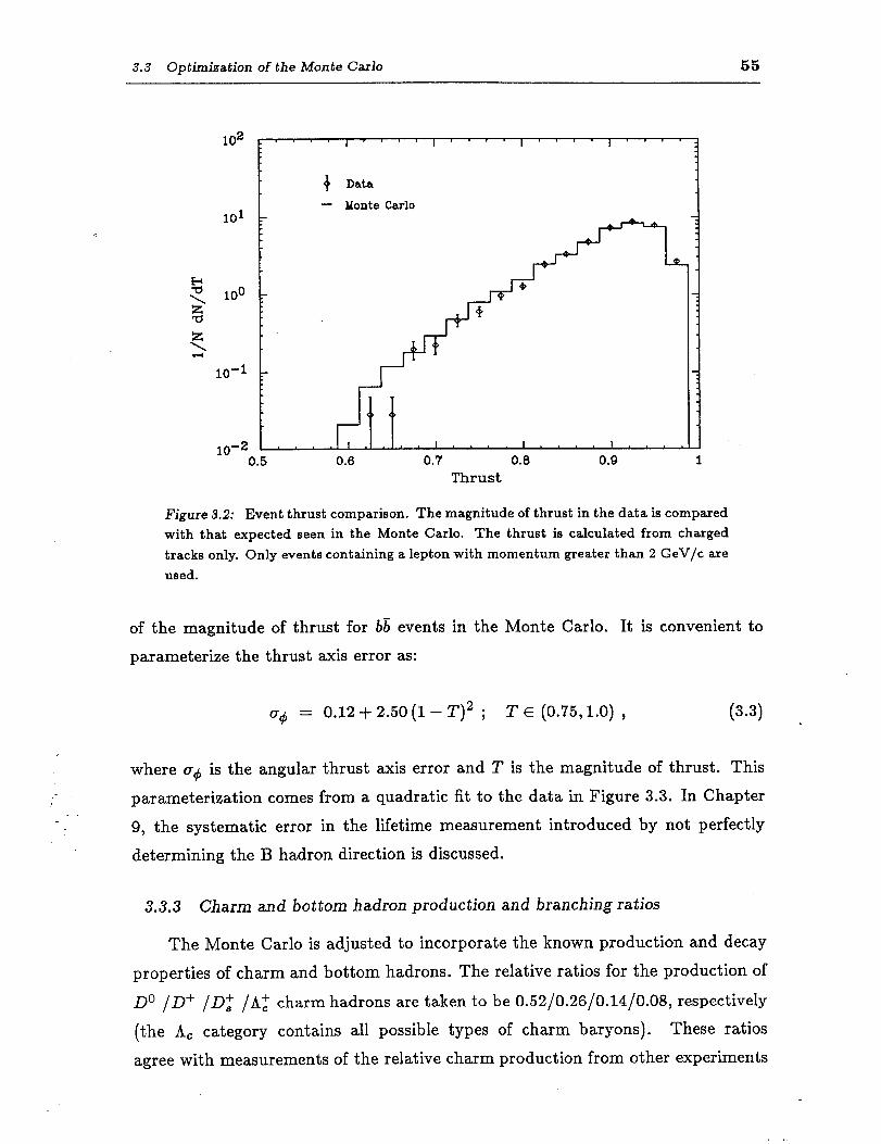
3.3 0ptixnil;ation of the Monte Carlo 55
0.7 0.8 0.9 1 Thrust
Figure 3.2: Event thrust comparison. The magnitude of thrust in the data is compared with that expected seen in the Monte Carlo. The thrust is calculated from charged tracks only. Only events containing a lepton with momentum greater than 2 GeV/c are used.
of the magnitude of thrust for b6 events in the Monte Carlo. It is convenient to
parameterize the thrust axis error as:
a4 = 0.12 + 2.50(1 - T)2 ; T E (0.75,l.O) , (3 3) .
where a+ is the angular thrust axis error and T is the magnitude of thrust. This
parameterization comes from a quadratic fit to the data in Figure 3.3. In Chapter
9, the systematic error in the lifetime measurement introduced by not perfectly
determining the B hadron direction is discussed.
3.3.3 Charm and bottom hadron production and branching ratios
The Monte Carlo is adjusted to incorporate the known production and decay
properties of charm and bottom hadrons. The relative ratios for the production of
Do /D’ /Dz /AZ charm hadrons are taken to be 0.52/0.26/0.14/0.08, respectively
(the A, category contains all possible types of charm baryons). These ratios
agree with measurements of the relative charm production from other experiments
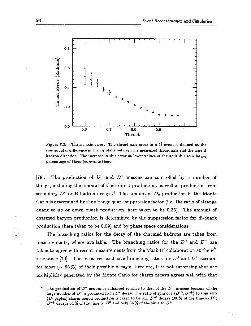
56 Event Reconstruction and Simulation
0.0” ’ ’ ’ ’ ’ ’ ’ ’ ’ ’ ’ ’ ’ ’ ’ ’ ’ ’ ’ ’ ’ ’ ’ 1-J 0.6 0.7 0.8 0.9 1
Thrust
Figure 3.3: Thrust axis error. The thrust axis error in a bg event is defined as the rms angular difference in the xy plane between the measured thrust axis and the true B hadron direction. The increase in this error at lower values of thrust is due to a larger percentage of three jet events there.
[78]. The production of Do and D+ mesons are controlled by a number of
things, including the amount of their direct production, as well as production from
secondary D* or B hadron decays. * The amount of D, production in the Monte
Carlo is determined by the strange quark suppression factor (i.e. the ratio of strange
quark to up or down quark production, here taken to be 0.33). The amount of
charmed baryon production is determined by the suppression factor for di-quark
production (here taken to be 0.09) and by phase space considerations.
The branching ratios for the. decay of the charmed hadrons are taken from
measurements, where available. The branching ratios for the Do and D+ are
taken to agree with recent measurements from the Mark III collaboration at the $J”
resonance [79]. The measured exclusive branching ratios for Do and D+ account
for most (- 85 %) of their possible decays; therefore, it is not surprising that the
multiplicity generated by the Monte Carlo for charm decays agrees well with that
* The production of Do mesons is enhanced relative to that of the D+ mesons because of the large number of Do ‘s produced from D* decay. The ratio of spin one (D*O, D*+) to spin zero (Do ,dplus) charm meson production is taken to be 3:l. D*O decays 100 % of the time to Do; D*+ decays 64 % of the time to Do and only 36 % of the time to D+.
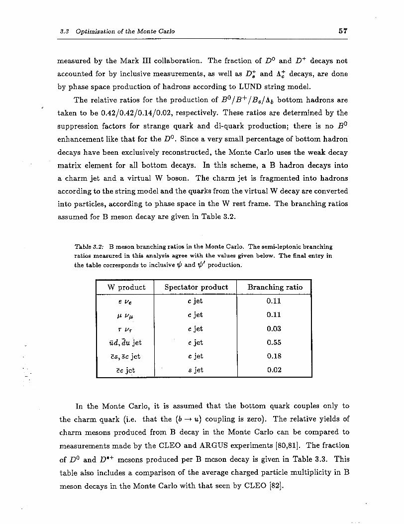
3.3 Optimization of the Monte Carlo 57
measured by the Mark III collaboration. The fraction of Do and D+ decays not
accounted for by inclusive measurements, as well as 0: and AZ decays, are done
by phase space production of hadrons according to LUND string model.
The relative ratios for the production of B’/B+/B,/Ab bottom hadrons are c
taken to be 0.42/0.42/0.14/0.02, respectively. These ratios are determined by the
suppression factors for strange quark and di-quark production; there is no B”
enhancement like that for the Do. Since a very small percentage of bottom hadron
decays have been exclusively reconstructed, the Monte Carlo uses the weak decay
matrix element for all bottom decays. In this scheme, a B hadron decays into
a charm jet and a virtual W boson. The charm jet is fragmented into hadrons
according to the string model and the quarks from the virtual W decay are converted
into particles, according to phase space in the W rest frame. The branching ratios
assumed for B meson decay are given in Table 3.2.
Table 3.2: B meson branching ratios in the Monte Carlo. The semi-leptonic branching ratios measured in this analysis agree with the values given below. The final entry in the table corresponds to inclusive $J and $J’ production.
v W product Spectator product Branching ratio
e Ye c jet 0.11
p VP c jet 0.11
7- VT c jet 0.03
iid,& jet c jet 0.55
Es,Sc jet c jet 0.18
EC jet s jet 0.02
In the Monte Carlo, it is assumed that the bottom quark couples only to
the charm quark (i.e. that the (b + u) coupling is zero). The relative yields of
charm mesons produced from B decay in the Monte Carlo can be compared to
measurements made by the CLEO and ARGUS experiments [80,81]. The fraction
of Do and II*+ mesons produced per B meson decay is given in Table 3.3. This
table also includes a comparison of the average charged particle multiplicity in B
meson decays in the Monte Carlo with that seen by CLEO [82].
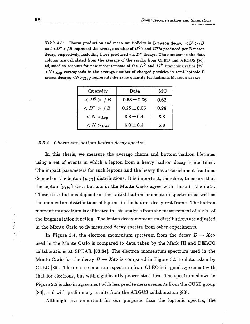
58 Event Reconstruction and Simulation
c
Table 3.3: Charm production and mean multiplicity in B meson decay. <Do> /a and <D+> /B represent the average number of Do’s and D+‘s produced per B meson
decay, respectively, including those produced via D* decays. The numbers in the data column are calculated from the average of the results from CLEO and ARGUS [80], adjusted to account for new measurements of the Do and D+ branching ratios [79]. <N>L~~ corresponds to the average number of charged particles in semi-leptonic B
meson decays; <N>Had represents the same quantity for hadronic B meson decays.
I Quantity I Data I MC
<Do> fB 0.58 III 0.06 0.62
<D+> fB 0.25 AI 0.05 0.28
< N >~e~ 3.8 310.4 3.8
<N )Had 6.0 310.3 5.8
3.3.4 Charm and bottom hadron decay spectra
In this thesis, we measure the average charm and bottom’hadron lifetimes
using a set of events in which a lepton from a heavy hadron decay is identified.
The impact parameters for such leptons and the heavy flavor enrichment fractions
depend on the lepton (p,pt) distributions. It is important, therefore, to ensure that
the lepton (P,P~) distributions in the Monte Carlo agree with those in the data.
These distributions depend on the initial hadron momentum spectrum as well as
the momentum distributions of leptons in the hadron decay rest frame. The hadron
momentum spectrum is calibrated in this analysis from the measurement of < x > of
the fragmentation function. The lepton decay momentum distributions are adjusted
in the Monte Carlo to fit measured decay spectra from other experiments.
In Figure 3.4, the electron momentum spectrum from the decay D + Xev
used in the Monte Carlo is compared to data taken by the Mark III and DELCO
collaborations at SPEAR [83,84]. Th e electron momentum spectrum used in the
Monte Carlo for the decay B + Xev is compared in Figure 3.5 to data taken by
CLEO [85]. Th e muon momentum spectrum from CLEO is in good agreement with
that for electrons, but with significantly poorer statistics. The spectrum shown in
Figure 3.5 is also in agreement with less precise measurements from the CUSB group
[86], and with preliminary results from the ARGUS collaboration [80].
Although less important for our purposes than the leptonic spectra, the
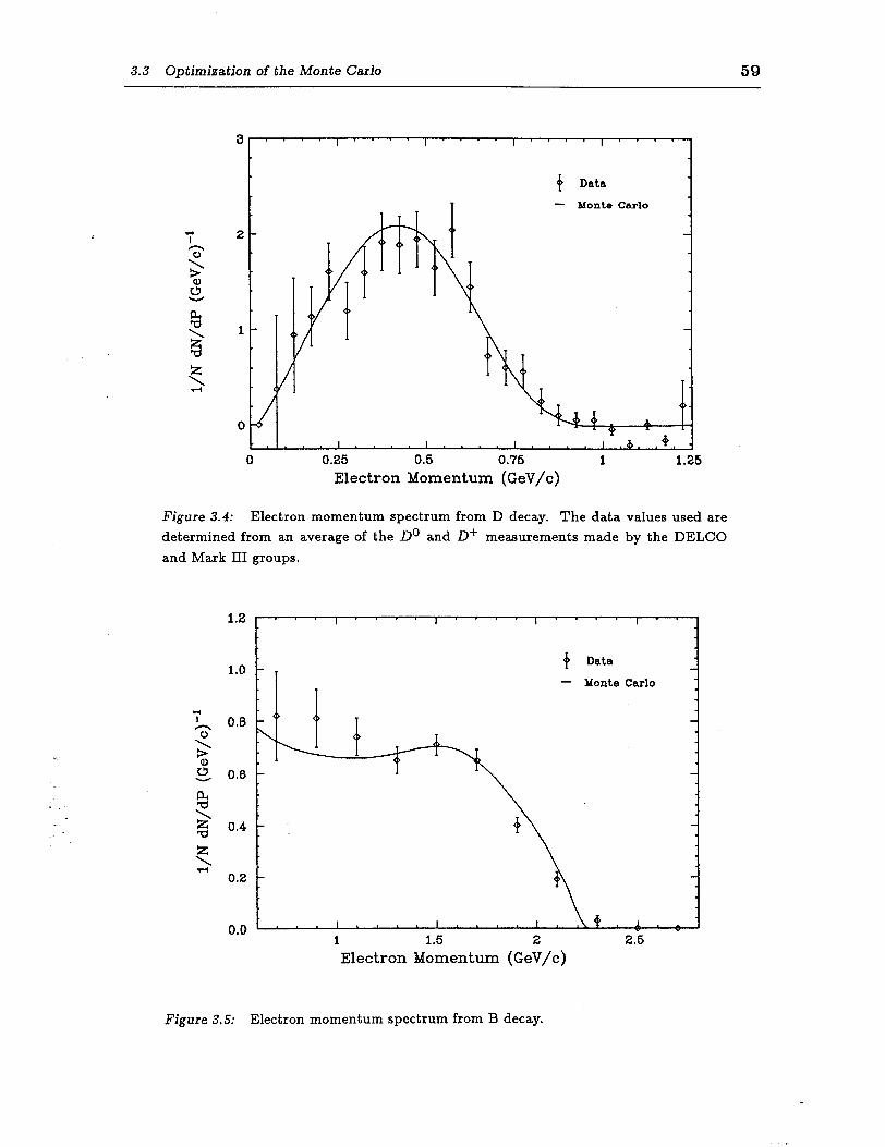
3.3 Optimization of the Monte Carlo 59
0.25 0.5 0.76 Electron Momentum (GeV/c)
Figure 3.4: Electron momentum spectrum from D decay. The data values used are determined from an average of the Do and D+ measurements made by the DELCO and Mark III groups.
% \ $j 0.4
5 0.2
0.0 1 1.5 2
Electron Momentum (GeV/c)
FiFure 3.5: Electron momentum spectrum from B decay.
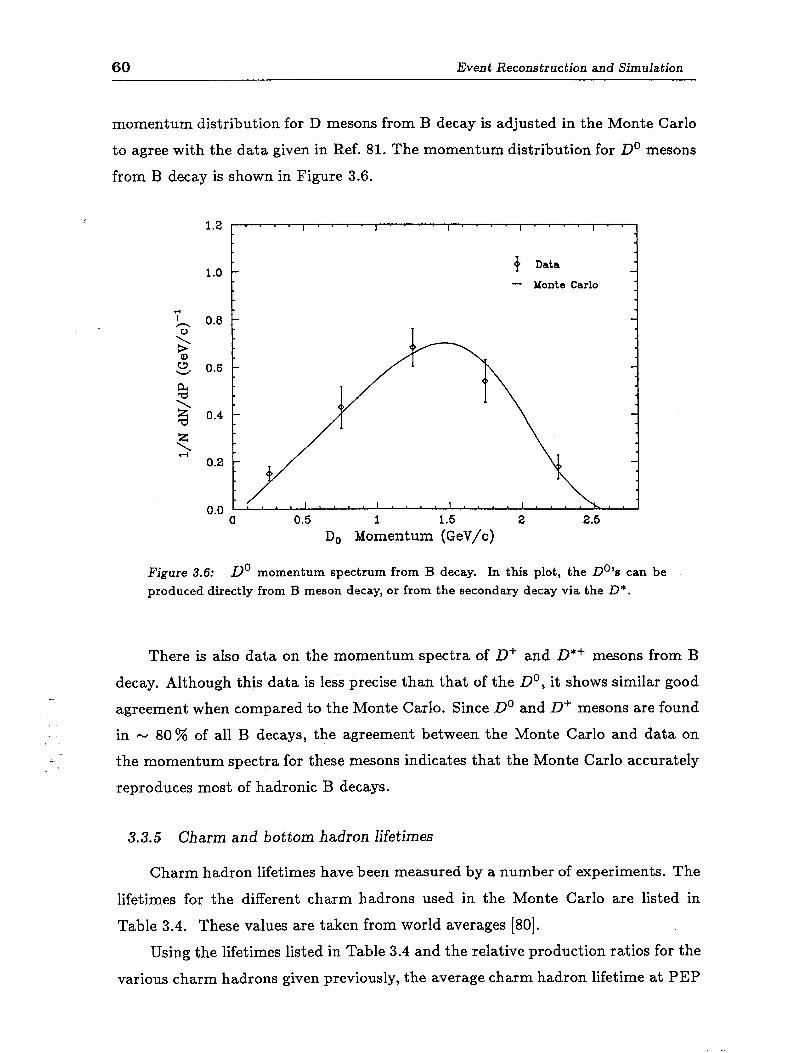
60 Event Reconstruction and Simulation
momentum distribution for D mesons from B decay is adjusted in the Monte Carlo
to agree with the data given in Ref. 81. The momentum distribution for Do mesons
from B decay is shown in Figure 3.6.
1.2
0.8
0.6
0.5 1 1.5 2 2.5 DO Momentum (GeV/c)
Figure 3.6: Do momentum spectrum from B decay. In this plot, the Do’s can be I produced directly from B meson decay, or from the secondary decay via the D*.
There is also data on the momentum spectra of D+ and D*+ mesons from B
decay. Although this data is less precise than that of the Do, it shows similar good
agreement when compared to the Monte Carlo. Since Do and D+ mesons are found
in - 80 % of all B decays, the agreement between the Monte Carlo and data on
the momentum spectra for these mesons indicates that the Monte Carlo accurately
reproduces most of hadronic B decays.
3.3.5 Charm and bottom hadron lifetimes
Charm hadron lifetimes have been measured by a number of experiments. The
lifetimes for the different charm hadrons used in the Monte Carlo are listed in
Table 3.4. These values are taken from world averages [80].
Using the lifetimes listed in Table 3.4 and the relative production ratios for the
various charm hadrons given previously, the average charm hadron lifetime at PEP
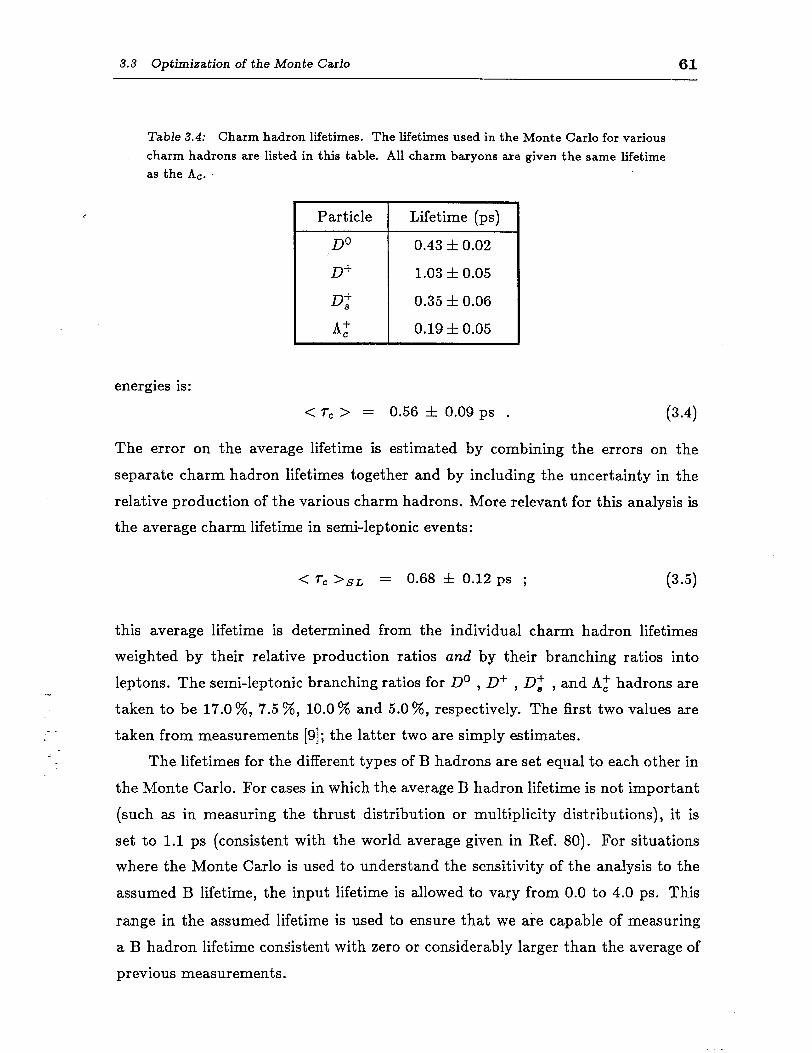
3.3 Optimization of the Monte Carlo 61
Table 3.4: Charm hadron lifetimes. The lifetimes used in the Monte Carlo for various charm hadrons are listed in this table. All charm baryons are given the same lifetime as the AC.
Particle
DO
D+
Dt
A:
Lifetime (ps)
0.43 & 0.02
1.03 rfr 0.05
0.35 zt 0.06
0.19 Zt 0.05
energies is:
CT,> = 0.56 rt 0.09 ps . (3 4) .
The error on the average lifetime is estimated by combining the errors on the
separate charm hadron lifetimes together and by including the uncertainty in the
relative production of the various charm hadrons. More relevant for this analysis is
the average charm lifetime in semi-leptonic events:
< Tc )SL = 0.68 zt 0.12 ps ; ( 5) 3.
this average lifetime is determined from the individual charm hadron lifetimes
weighted by their relative production ratios and by their branching ratios into
leptons. The semi-leptonic branching ratios for Do , D+ , 0: , and AZ hadrons are
taken to be 17.0%, 7.5 %, 10.07 o and 5.0 %, respectively. The first two values are
taken from measurements [9]; the latter two are simply estimates.
The lifetimes for the different types of B hadrons are set equal to each other in
the Monte Carlo. For cases in which the average B hadron lifetime is not important
(such as in measuring the thrust distribution or multiplicity distributions), it is
set to 1.1 ps (consistent with the world average given in Ref. 80). For situations
where the Monte Carlo is used to understand the sensitivity of the analysis to the
assumed B lifetime, the input lifetime is allowed to vary from 0.0 to 4.0 ps. This
range in the assumed lifetime is used to ensure that we are capable of ‘measuring
a B hadron lifetime consistent with zero or considerably larger than the average of
previous measurements.

62
Chapter 4
Tracking and Resolution Studies
In this chapter the precision tracking of charged particles in the Mark II
detector is discussed. Tracking of this type depends almost completely on the
performance and position resolution of the Vertex Chamber. This chapter presents
a complete description of the issues relevant to VC tracking.
The method by which tracking in the Vertex Chamber is decoupled from
that in the Drift Chamber is first discussed. A number of improvements to the
tracking procedure are outlined; these improvements result from a careful chamber
survey made via wire residual distributions. From a study of the distributions of
track x2 values and impact parameters, it is shown that the VC resolution is well
understood for isolated tracks and for tracks in hadronic events. Understanding the
resolution for this latter set of tracks is vital because such tracks are used in the
lifetime determination.
4.1 Vertex Chamber Tracking
The basic tracking procedure treats the Vertex Chamber and Drift Chamber
as a single large system. Although this procedure is optimal in determining track
momenta and in finding tracks with high efficiency, it does not provide the most
accurate tracking in regard to position resolution. Any geometrical aberrations in
the DC, or in the relative alignment between the VC and DC can translate into
increased (systematic) error in extrapolating tracks to the origin. For that reason,
after the track-finding procedure is applied, tracks are refit by an algorithm which
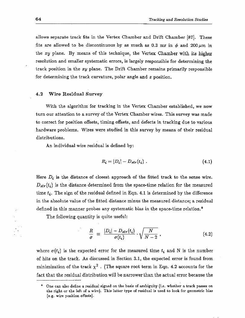
64 ?Iracking and Resolution Studies
allows separate track fits in the Vertex Chamber and Drift Chamber [87]. These
fits are allowed to be discontinuous by as much as 0.3 mr in 4 and 200~.4m in
the zy plane. By means of this technique, the Vertex Chamber with its higher
resolution and smaller systematic errors, is largely responsible for determining the
track position in the sy plane. The Drift Chamber remains primarily responsible
for determining the track curvature, polar angle and z position.
4.2 Wire Residual Survey
With the algorithm for tracking in the Vertex Chamber established, we now
turn our attention to a survey of the Vertex Chamber wires. This survey was made
to correct for position offsets, timing offsets, and defects in tracking due to various
hardware problems. Wires were studied in this survey by means of their residual
distributions.
An individual wire residual is defined by:
R; = IDil -D&i) l
Here Di is the distance of closest approach of the fitted track to the sense wire.
Dstr(tJ is the distance determined from the space-time relation for the measured
time t;. The sign of the residual defined in Eqn. 4.1 is determined by the difference
in the absolute value of the fitted distance minus the measured distance; a residual
defined in this manner probes any systematic bias in the space-time relation.*
The following quantity is quite useful:
R = ID;1 - at?&) N - . CT - 4i> r- N-2’
where a(tJ is the expected error for the measured time t; and N is the number
of hits on the track. As discussed in Section 3.1, the expected error is found from
minimization of the track x2 . (The square root term in Eqn. 4.2 accounts for the
fact that the residual distribution will be narrower than the actual error because the
* One can also define a residual signed on the basis of ambiguity (i.e. whether a track passes on the right or the left of a wire). This latter type of residual is used to look for geometric bias (e.g. wire position offsets).
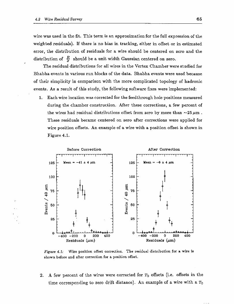
4.2 Wire Residual Survey 65
wire was used in the fit. This term is an approximation for the full expression of the
weighted residuals). If there is no bias in tracking, either in offset or in estimated
error, the distribution of residuals for a wire should be centered on zero and the
distribution of % should be a unit width Gaussian centered on zero.
The residual distributions for all wires in the Vertex Chamber were studied for
Bhabha events in various run blocks of the data. Bhabha events were used because
of their simplicity in comparison with the more complicated topology of hadronic
events. As a result of this study, the following software fixes were implemented:
1. Each wire location was corrected for the feedthrough hole positions measured
during the chamber construction. After these corrections, a few percent of
the wires had residual distributions offset from zero by more than -25 pm .
These residuals became centered on zero after corrections were applied for
wire position offsets. An example of a wire with a position offset is shown in
Figure 4.1.
Before Correction
0 -400 -200 0 200 400
Residuals (pm)
After Correction
~“““““““““““‘~
125 -
100 -
I.
3 75 -
\ 2 !I 50 -
& 25 -
Mean = -6*4/&m
+ 0 I, L ,A6
-400 -200 0 200 400 Residuals (pm)
Figure 4.1: Wire position offset correction. The residual distribution for a wire is shown before and after correction for a position offset.
2. A few percent of the wires were corrected for ~0 offsets (i.e. offsets in the
time corresponding to zero drift distance). An example of a wire with a ‘1”0
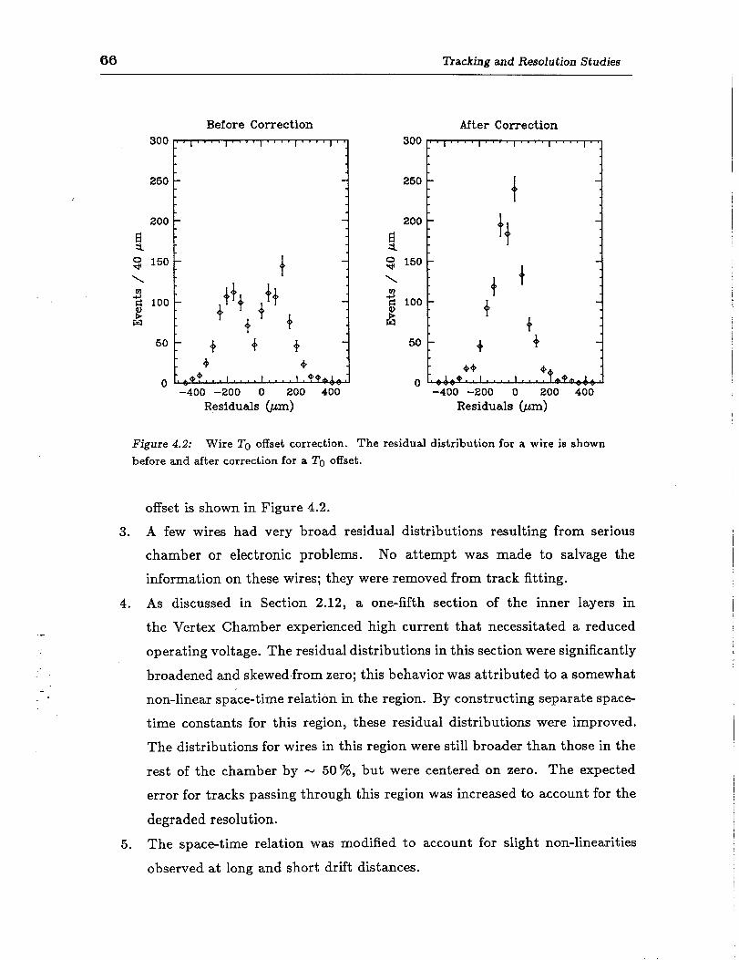
66 ZIacking and Resolution Studies
250
Before Correction
-400 -200 0 200 460 Residuals (pm)
After Correction
250
F 200 -
1 $ 150 - \
2 100 - g! w
50 - +
0 -400 -200 0 200 400
Residuals bm)
Figure 4.2: Wire TO offset correction. The residual distribution for a wire is shown before and after correction for a To offset.
offset is shown in Figure 4.2.
3. A few wires had very broad residual distributions resulting from serious
chamber or electronic problems. No attempt was made to salvage the
information on these wires; they were removed from track fitting.
4. As discussed in Section 2.12, a one-fifth section of the inner layers in
the Vertex Chamber experienced high current that necessitated a reduced
operating voltage. The residual distributions in this section were significantly
broadened and skewed from zero; this behavior was attributed to a somewhat
non-linear space-time relation in the region. By constructing separate space-
time constants for this region, these residual distributions were improved.
The distributions for wires in this region were still broader than those in the
rest of the chamber by - 50 %, but were centered on zero. The expected
error for tracks passing through this region was increased to account for the
degraded resolution.
5. The space-time relation was modified to account for slight non-linearities
observed at long and short drift distances.
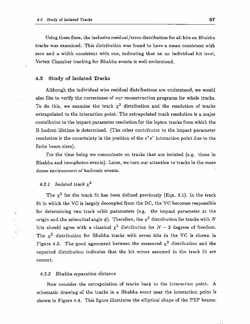
4.3 Study of Isolated llacks 67
Using these fixes, the inclusive residual/error distribution for all hits on Bhabha
tracks was examined. This distribution was found to have a mean consistent with
zero and a width consistent with one, indicating that on an individual hit level,
Vertex Chamber tracking for Bhabha events is well understood.
4.3 Study of Isolated Tracks
Although the individual wire residual distributions are understood, we would
also like to verify the correctness of our reconstruction programs for whole tracks.
To do this, we examine the track x2 distribution and the resolution of tracks
extrapolated to the interaction point. The extrapolated track resolution is a major
contributor to the impact parameter resolution for the lepton tracks from which the
B hadron lifetime is determined. (The other contributor to the impact parameter
resolution is the uncertainty in the position of the e+e- interaction point due to the
finite beam sizes).
For the time being we concentrate on tracks that are isolated (e.g. those in
Bhabha and two-photon events). Later, we turn our attention to tracks in the more
dense environment of hadronic events.
4.3.1 Isolated track x2
The x2 for the track fit has been defined previously (Eqn. 3.1). In the track
fit in which the VC is largely decoupled from the DC, the VC becomes responsible
for determining two track orbit parameters (e.g. the impact parameter at the
origin and the azimuthal angle 4). Therefore, the x2 distribution for tracks with N
hits should agree with a classical x2 distribution for N - 2 degrees of freedom.
The x2 distribution for Bhabha tracks with seven hits in the VC is shown in
Figure 4.3. The good agreement between the measured x2 distribution and the
expected distribution indicates that the hit errors assumed in the track fit are
correct.
4.3.2 Bhabha separation distance
Now consider the extrapolation of tracks back to the interaction point, A
schematic drawing of the tracks in a Bhabha event near the interaction point is
shown in Figure 4.4. This figure illustrates the elliptical shape of the PEP beams.
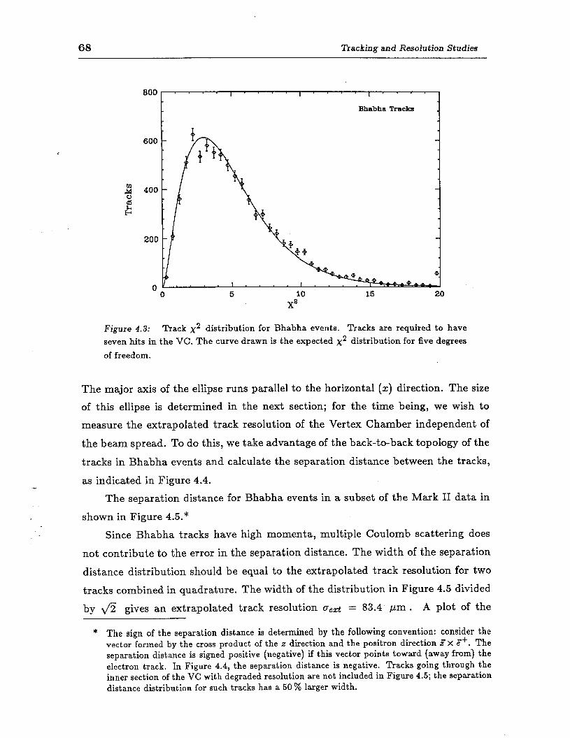
68 ?‘racking and Resolution Studies
Figure 4.3: Track x2 distribution for Bhabha events. Tracks are required to have seven hits in the VC. The curve drawn is the expected x2 distribution for five degrees of freedom.
The major axis of the ellipse runs parallel to the horizontal (z) direction. The size
of this ellipse is determined in the next section; for the time being, we wish to
measure the extrapolated track resolution of the Vertex Chamber independent of
the beam spread. To do this, we take advantage of the back-to-back topology of the
tracks in Bhabha events and calculate the separation distance between the tracks,
as indicated in Figure 4.4.
The separation distance for Bhabha events in a subset of the Mark II data in
shown in Figure 4.5.*
Since Bhabha tracks have high momenta, multiple Coulomb scattering does
not contribute to the error in the separation distance. The width of the separation
distance distribution should be equal to the extrapolated track resolution for two
tracks combined in quadrature. The width of the distribution in Figure 4.5 divided
by 4 gives an extrapolated track resolution oezt = 83.4 ,um . A plot of the
* The sign of the separation distance is determined by the following convention: consider the vector formed by the cross product of the z direction and the positron direction z’ x e ++. The separation distance is signed positive (negative) if this vector points toward (away from) the electron track. In Figure 4.4, the separation distance is negative. Tracks going through the inner section of the VC with degraded resolution are not included in Figure 4.5; the separation distance distribution for such tracks has a 50 % larger width.
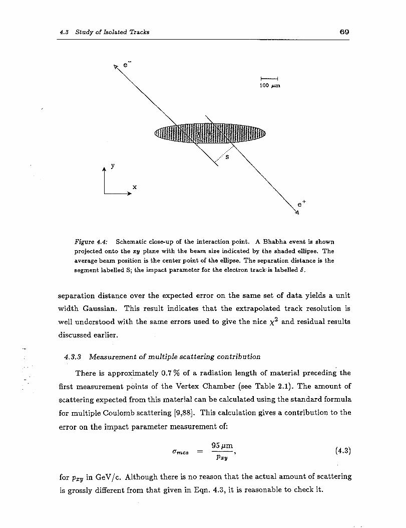
4.3 Study of Isolated Tracks 69
e- 9
Y
L X
I I 100 pm
Figure 4.4: Schematic close-up of the interaction point. A Bhabha event is shown projected onto the zy plane with the beam size indicated by the shaded ellipse. The average beam position is the center point of the ellipse. The separation distance is the segment labelled S; the impact parameter for the electron track/is labelled 6.
separation distance over the expected error on the same set of data yields a unit
width Gaussian. This result indicates that the extrapolated track resolution is
well understood with the same errors used to give the nice x2 and residual results
discussed earlier.
4.3.3 Measurement of multiple scattering contribution
There is approximately 0.7 % of a radiation length of material preceding the
first measurement points of the Vertex Chamber (see Table 2.1). The amount of
scattering expected from this material can be calculated using the standard formula
for multiple Coulomb scattering [9,88]. This calculation gives a contribution to the
error on the impact parameter measurement of:
95 ,um gmcs =
Pxy ’ (4 3) .
for pzy in GeV/c. Although there is no reason that the actual amount of scattering
is grossly different from that given in Eqn. 4.3, it is reasonable to check it.

70 Tracking and Resolution Studies
Bhabha Tracks 1
10-l -1 -0.5 0 0.5 1
Separation Distance (mm)
Figure 4.5: Bhabha separation distance. Tracks in this plot are required to have at least four VC hits and a track x2 probability fit larger than 0.1%. The curve drawn corresponds to a Gaussian fit to the data out to f3 standard deviations.
The amount of scattering can been determined by measuring the impact
parameter distribution for tracks in two-photon scattering events. In this
measurement, events of the type e+e- + e+e-e+e- and e+e- + e+e-p$- are
used, where two leptons are scattered into the central detector and the other two
escape along the beam axis. The criteria for selecting events of this type have been
described previously [89]. These events are chosen because they contain tracks
produced at the interaction point (i.e. there is no lifetime bias). The tracks are
at low momenta and are well isolated, enhancing the amount of scattering and
permitting quality tracking, respectively.
The impact parameter 6 of each track that passes minimum quality cuts is
measured in the xy plane with respect to the beam position. The event axis is
determined by the momentum sum of the two tracks in the central detector. The
sign of the impact parameter is determined by whether a track crosses the event
axis at a point in the same hemisphere as the track (f), or at a point in the opposite
hemisphere (-). B ecause the momentum sum of the two tracks in the xy plane is
close to zero, this method effectively randomizes the sign. In order to maximize the
contribution of multiple Coulomb scattering to the impact parameter error, only
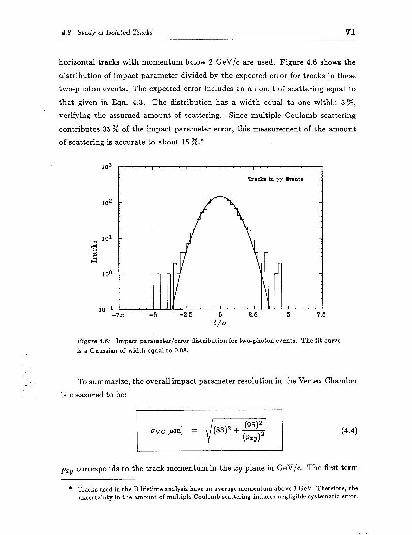
4.3 Study of Isolated Tracks 71
horizontal tracks with momentum below 2 GeV/c are used. Figure 4.6 shows the
distribution of impact parameter divided by the expected error for tracks in these
two-photon events. The expected error includes an amount of scattering equal to
that given in Eqn. 4.3. The distribution has a width equal to one within 5 %, c
verifying the assumed amount of scattering. Since multiple Coulomb scattering
contributes 35 % of the impact parameter error, this measurement of the amount
of scattering is accurate to about 15 %.*
103
Tracks in ry Events
-2.5 0 2.5 5 7.5
vu
Figure 4.6: Impact parameter/error distribution for two-photon events. The fit curve is a Gaussian of width equal to 0.98.
To summarize, the overall impact parameter resolution in the Vertex Chamber
is measured to be:
(4 4) .
pZY corresponds to the track momentum in the zy plane in GeV/c. The first term
* Tracks used in the B lifetime analysis have an average momentum above 3 GeV. Therefore, the uncertainty in the amount of multiple Coulomb scattering induces negligible systematic error.
72 Tracking and Resolution Studies
in Eqn. 4.4 is the intrinsic extrapolated track resolution of the Vertex Chamber; the
second term is the contribution to the resolution from multiple Coulomb scattering.
4.4 Beam Parameters
4.4.1 Beam position determination
The technique for determining the average beam position has been described
in another thesis [55]. This technique looks at the average intersection point of
- good tracks taken from blocks of ten to twenty runs (typically several days). Tracks
within a few degrees of the vertical (horizontal) direction determine the horizontal
(vertical) position of the beam. The statistical error on the location of the beam
position determined by this method is - 15 Grn in both z and y.
This method of beam position determination requires data from a large number
of runs. Therefore, its accuracy could be compromised if there was a significant
amount of beam steering between fills of the PEP machine. To study the effects
of beam steering between runs, an algorithm for determining the beam position
within a single run was developed [58]. Th is algorithm uses all the good tracks
in a run; it determines the beam position by minimizing the impact parameters
for the entire ensemble of tracks. Beam positions are determined by this method
with a statistical precision of - 2Opm in the vertical direction and - 5Opm in the
horizontal direction. There is good agreement between the two different estimates
of the beam positions. In addition, as outlined in Section 2.3, blocks of data having
excessive beam motion within a run are eliminated by using the information from
the hardware Beam Position Monitor.
The impact parameter distribution for Bhabha tracks provides a useful check
on the azimuthal symmetry of the Vertex Chamber and on the accuracy of beam
position determination. In Figure 4.7, the mean Bhabha impact parameter is
plotted as a function of the azimuthal angle 4. The impact parameter is defined to
be positive (negative) if the vector formed from the cross product of the z direction
and the track direction points toward (away from) the beam position. On the scale
of - 20 pm, no angular dependence of the mean impact parameter is observed.
4.4.2 Beam size determination
The PEP vertical and horizontal beam sizes are determined from the
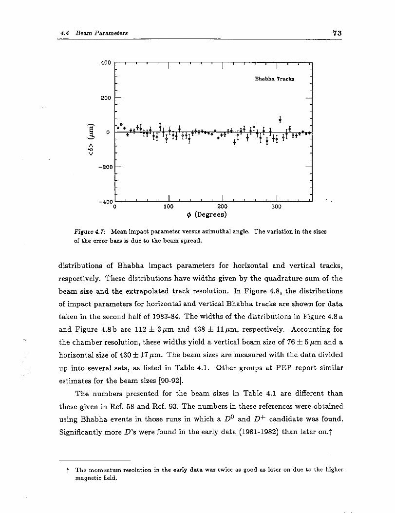
4.4 Beam Parameters 73
400. I I I I 1 I 1 I I II I I I I I’
Bhabha Tracks
200 -
-400 I I I I I I I I I I t I 0 100 200 300
9 (Degrees)
Figure 4.7: Mean impact parameter versus azimuthal angle. The variation in the sizes of the error bars is due to the beam spread.
distributions of Bhabha impact parameters for horizontal and vertical tracks,
respectively. These distributions have widths given by the quadrature sum of the
beam size and the extrapolated track resolution. In Figure 4.8, the distributions
of impact parameters for horizontal and vertical Bhabha tracks are shown for data
taken in the second half of 1983-84. The widths of the distributions in Figure 4.8 a
and Figure 4.8 b are 112 & 3pm and 438 It 11 pm, respectively. Accounting for
the chamber resolution, these widths yield a vertical beam size of 76 & 5 pm and a
horizontal size of 430 & 17pm. The beam sizes are measured with the data divided
up into several sets,- as listed in Table 4.1. Other groups at PEP report similar
estimates for the beam sizes [90-921.
The numbers presented for the beam sizes in Table 4.1 are different than
those given in Ref. 58 and Ref. 93. The numbers in these references were obtained
using Bhabha events in those runs in which a Do and D+ candidate was found.
Significantly more D’s were found in the early data (1981-1982) than later on.t
t The momentum resolution in the early data was twice as good as later on due to the higher magnetic field.
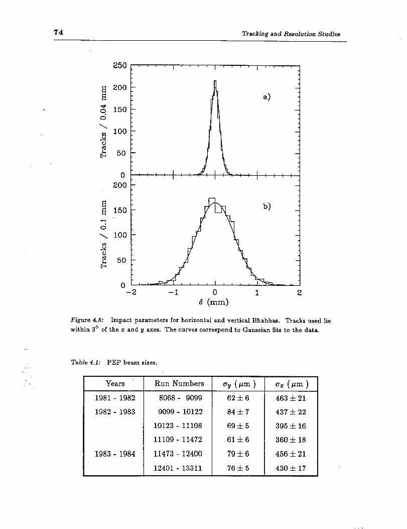
74 Tracking and Resolution Studies
E E
250
200
150
100
50
0 200
150
100
50
0
Figure 4.8: Impact parameters for horizontal and vertical Bhabhas. Tracks used lie within 3’ of the 51: and y axes. The curves correspond to Gaussian fits to the data.
Table 4.1: PEP beam sizes.
I Years I Run Numbers OY (J-4 ax (Pm) 1981- 1982
1982 - 1983
1983 - 1984
8068- 9099 62zk6 463rfr21
9099- 10122 84zk 7 437zk22
10123 - 11108 69zt5 395zkl6
11109- 11472 6lzt6 36Ortl8
11473 - 12400 79 k 6 456 It: 21
12401- 13311 7655 43ozk17
4.5 Study of Tracks in Hadronic Events 75
4.5 Study of Tracks in Hadronic Events
The Mark II Vertex Chamber has a double track resolution of - 5mm,*
approximately equal to the VC cell size. W ith the measurement points in the c
first layer of the VC at an average radius of 11 cm, this double track resolution
translates into an angular resolution of 45 m r. In hadronic events at PEP energies,
the average angular separation between a charged track and its nearest neighbor
is - 160 m r, but about one quarter of the tracks have another track within 50
- m r. Therefore, the density of tracks in typical hadronic events often reaches the
maximum density in which the Vertex Chamber can efficiently reconstruct tracks.
A loss in tracking efficiency in a high density environment is expected. Since the
Monte Carlo is able to simulate much of this efficiency loss, only the difference
between the tracking efficiency in the data and in the Monte Carlo is of interest.
In this analysis, however, the systematic error in the lifetime measurement
due to the difference in tracking efficiency between the data and Monte Carlo is
small in comparison with the uncertainty in the shape of the resolution function.
Therefore, our main concern about tracking in a ‘dense environment is not the
track eficiency, but rather the quality of reconstuction. The bulk of this section is
devoted to understanding the tracking resolution in the Mark II Vertex Chamber
for hadronic events. We will see that the position resolution for tracks in hadronic
events is degraded by 25 % from that observed for isolated tracks. This degradation
is largely due to electronic cross-talk in the VC pre-amplifiers and although it cannot
be eliminated, it can be corrected for. At the end of this section, we return to the
question of track efficiency in hadronic events.
4.5.1 Hadronic track x2
The VC x2 distribution for tracks in hadronic events is shown in Figure 4.9.
There is a large disagreement between the x2 distribution observed in the data and
the expected distribution. “The disagreement is embarrassing” [55].
* The double track resolution defined here is the minimum distance two tracks must be separated so that they are both resolved with 90 % efficiency. The value of 5 m m is determined from a sample of 7 three prong decays.
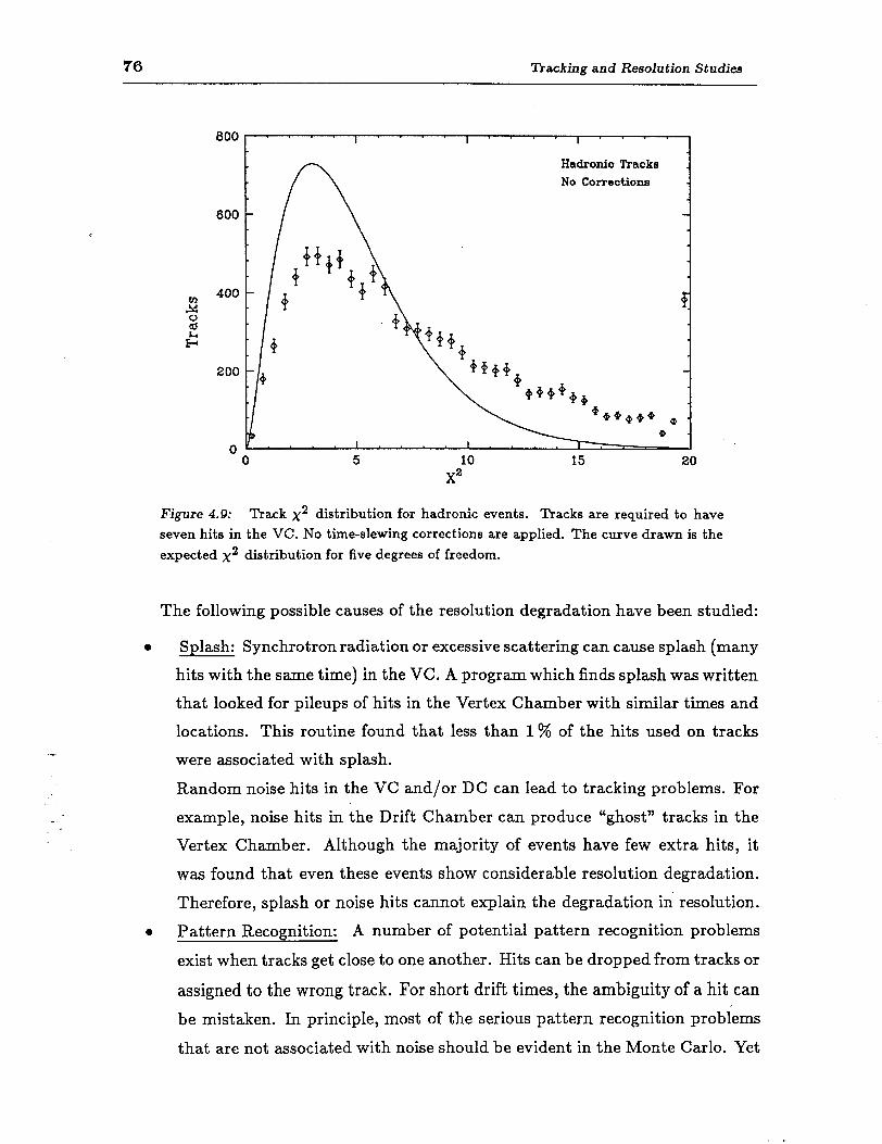
76 ?Iracking and Resolution Studies
600
4 400
2 &
200
0
Hedronic Tracks No Corrections
0 5 10 15 20 X2
Figure 4.9: Track x2 distribution for hadronic events. Tracks are required to have seven hits in the VC. No time-slewing corrections are applied. The curve drawn is the expected x2 distribution for five degrees of freedom.
The following possible causes of the resolution degradation have been studied:
0 Synchrotron radiation or excessive scattering can cause splash (many Splash:
hits with the same time) in the VC. A program which finds splash was written
that looked for pileups of hits in the Vertex Chamber with similar times and
locations. This routine found that less than 1% of the hits used on tracks
were associated with splash.
Random noise hits in the VC and/or DC can lead to tracking problems. For
example, noise hits in the Drift Chamber can produce “ghost” tracks in the
Vertex Chamber. Although the majority of events have few extra hits, it
was found that even these events show considerable resolution degradation.
Therefore, splash or noise hits cannot explain the degradation in resolution.
l Pattern Recognition: A number of potential pattern recognition problems
exist when tracks get close to one another. Hits can be dropped from tracks or
assigned to the wrong track. For short drift times, the ambiguity of a hit can
be mistaken. In principle, most of the serious pattern recognition problems
that are not associated with noise should be evident in the Monte Carlo. Yet
4.5 Study of nacks in Hadronic Events 77
c
the track x2 distribution in the Monte Carlo shows excellent agreement with
the expected distribution, leading to the conclusion that pattern recognition
problems are insufficient to explain the degradation observed in the data.
0 Cross-talk: It is possible to have cross-talk in the electronics or in the
chamber itself (i.e. ionization from one cell leaking into an adjacent cell).
The chamber cross-talk is expected to be small from electrostatic studies,
and the pre-amplifier cross-talk was measured on the bench to be less than
1%. In order to check the amount of cross-talk, the distribution of time
differences between adjacent hits in the VC was examined. This distribution
should be triangular and centered on zero if no cross-talk existed.* A pile-up
of events at zero time difference would be evidence for large cross-talk. No
such evidence was observed, leading to the conclusion that cross-talk (of the
type in which an adjacent wire is caused to fire) is not the cause of resolution
degradation.
There is, however, a type of cross-talk somewhat more subtle than the usual
one discussed above. Imagine two adjacent wires both having real hits on them (i.e.
hits caused by the passage of a charged track). If a certain amount of capacitive or
inductive coupling exists between the signal on one wire and that on the other wire,
it is possible for the early hit to cause time slewing of the later hit. The slewing
might not fire the wire with the later arriving time, but cause its time to be shifted.
This type of cross-talk could cause significant degradation in the resolution of the
slewed time without causing that time to be dropped from the fit. To explore the
possibility of slewing effects, individual wire residual distributions were studied in
detail.
4.5.2 The time-slewing effect
The usefulness of wire residual distributions was demonstrated in Section 4.2.
In particular, the inclusive distribution of $ (see Eqn. 4.2) for all hits is a good
indicator of bias in the determination of residuals. This distribution for hits on
Bhabha tracks has a mean centered on zero and a width consistent with one. The
mean is also flat as a function of drift time.
* The drift t ime spectrum is essentially a uniform distribution. The difference between two uniform distributions is a triangular one.
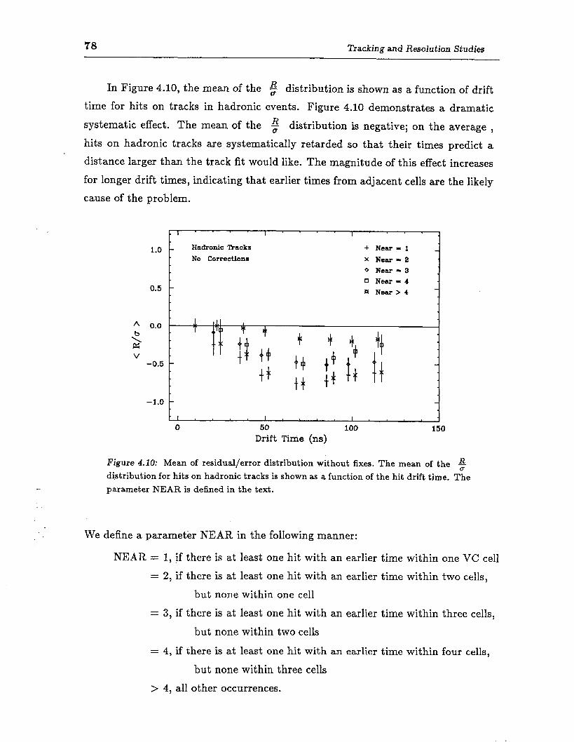
78 Tracking and Resolution Studies
In Figure 4.10, the mean of the $ distribution is shown as a function of drift time for hits on tracks in hadronic events. Figure 4.10 demonstrates a dramatic
systematic effect. The mean of the 5 distribution is negative; on the average , hits on hadronic tracks are systematically retarded so that their times predict a
distance larger than the track fit would like. The magnitude of this effect increases
for longer drift times, indicating that earlier times from adjacent cells are the likely
cause of the problem.
1.0
0.5
Kadronic Tracks
No Corrections
+ Near - 1
X Near - 2
0 Near - 3
•I Near - 4
# Near > 4
-1.0
0 50
Drift Time (ns) 100 150
Figure 4.10: Mean of residual/error distribution without fixes. The mean of the $ distribution for hits on hadronic tracks is shown as a function of the hit drift time. The parameter NEAR is defined in the text.
We define a parameter NEAR in the folIowing manner:
NEAR = 1, if there is at least one hit with an earlier time within one VC cell = 2, if there is at least one hit with an earlier time within two cells,
but none within one cell
= 3, if there is at least one hit with an earlier time within three cells,
but none within two cells
= 4, if there is at least one hit with an earlier time within four cells,
but none within three cells
> 4, all other occurrences.
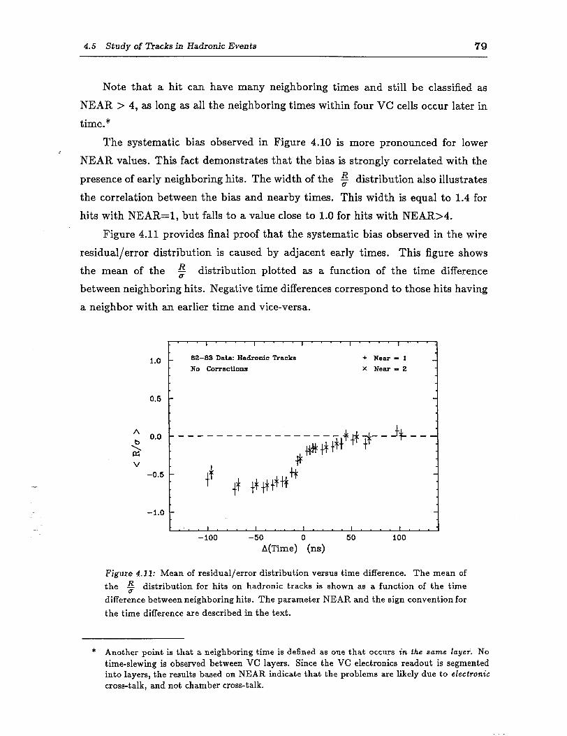
4.5 Study of Tracks in Hadronic Events 79
Note that a hit can have many neighboring times and still be classified as
NEAR > 4, as long as all the neighboring times within four VC cells occur later in
time.*
The systematic bias observed in Figure 4.10 is more pronounced for lower
NEAR values. This fact demonstrates that the bias is strongly correlated with the
presence of early neighboring hits. The width of the 5 distribution also illustrates
the correlation between the bias and nearby times. This width is equal to 1.4 for
hits with NEAR=l, but falls to a value close to 1.0 for hits with NEAR>4.
Figure 4.11 provides final proof that the systematic bias observed in the wire
residual/error distribution is caused by adjacent early times. This figure shows
the mean of the $ distribution plotted as a function of the time difference
between neighboring hits. Negative time differences correspond to those hits having
a neighbor with an earlier time and vice-versa.
1.0 -
0.5 -
^b 0.0 -
2
V -0.5 -
-1.0 -
82-83 Data: Hadronic Tracks + Near - 1
No Corrections x Near52
-----me--------- -4
t+
#++++hv- --
t
1
JlJE +JE ++t+t*
+#
i
t...1’..‘I”.‘I”“1”‘.“‘.1 -100 -50
A(Time) ’ (ns) 50 100
Figure 4.11: Mean of residual/error distribution versus time difference. The mean of the $ distribution for hits on hadronic tracks is shown as a function of the time difference between neighboring hits. The parameter NEAR and the sign convention for the time difference are described in the text.
* Another point is that a neighboring time is defined as one that occurs in the same layer. No time-slewing is observed between VC layers. Since the VC electronics readout is segmented into layers, the results based on NEAR indicate that the problems are likely due to electronic cross-talk, and not chamber cross-talk.
80 Tracking and Resolution Studies
The data points in Figure 4.11 lie on a curve that is remarkably similar to a
step function. The bias in the mean % is large and approximately constant for
hits with an early neighbor. This bias is greatly reduced for hits having a neighbor
with a later time.
4.5.3 Probable cause of the time-slewing effect
As discussed earlier, there are indications that the observed time-slewing effect
is due to electronic coupling. For a number of reasons, it was suspected that the
coupling took place at the pre-amplifier stage. There were oscillation problems in
the metal cage that housed the pre-amps and the board density was rather high in
this cage.
To investigate coupling effects in the pre-amps, a test circuit was set up to
simulate several parallel channels of readout. The time-slewing effect was observed
in this set-up. In particular, time-slewing only occurred for hits having an earlier
nearby hit when the transformer pre-amps (Figure 2.7) were used. The magnitude
of the slewing observed in the bench test was sufficient to explain the resolution
degradation in the data. A likely location for slewing is in the FE-8302 integrated
circuit on the transformer pre-amp boards. This IC consists of four individual
transformer circuits in a single 16 pin DIP package. The transformers share a
common core, allowing for inductive coupling. Another possible cause of coupling
is poor placement of ground returns. Without extensive lab work, it is impossible
to determine exactly where to lay the blame.
4.5.4 The fix to the time-slewing effect
The question now arises as to how to correct for the bias observed in the
% distribution, regardless of its origin. In principle, it would be nice to know
on a hit-by-hit basis exactly how much to correct for. The $ distribution
consists of an average of many hits, each which may be affected by the coupling in
varying amounts. This distribution is quite consistent, however, with a single offset
Gaussian; therefore, it is possible to treat the coupling in an average sense.
The fix to the time-slewing problem consists of the following recipe. All hits
are first categorized by NEAR. For each hit, an offset correction is applied to the
space-time relation, and the expected error on the hit is adjusted. These corrections
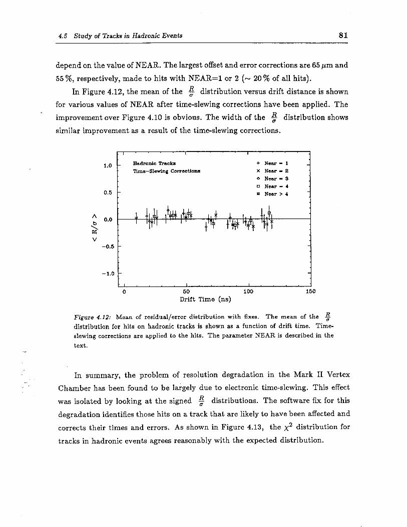
4.5 Study of 23acks in Hadronic Events 81
depend on the value of NEAR. The largest offset and error corrections are 65 pm and
55 %, respectively, made to hits with NEAR=1 or 2 (- 20 % of all hits).
In Figure 4.12, the mean of the 5 distribution versus drift distance is shown
for various values of NEAR after time-slewing corrections have been applied. The
improvement over Figure 4.10 is obvious. The width of the 5 distribution shows
similar improvement as a result of the time-slewing corrections.
1.0 Hadronic Tracks + Near = 1
Time-Slewing Corrections X Near = 2
0 Near - 3
0 Near - 4
0.5 # Near > 4
/
A 0.0
s V
-0.5
-1.0
50 Drift Time (ns)
Figure 4.12: Mean of residual/error distribution with fixes. The mean of the 5 distribution for hits on hadronic tracks is shown as a function of drift time. Time- slewing corrections are applied to the hits. The parameter NEAR is described in the text.
In summary, the problem of resolution degradation in the Mark II Vertex
Chamber has been found to be largely due to electronic time-slewing. This effect
was isolated by looking at the signed % distributions. The software fix for this
degradation identifies those hits on a track that are likely to have been affected and
corrects their times and errors. As shown in Figure 4.13, the x2 distribution for
tracks in hadronic events agrees reasonably with the expected distribution.
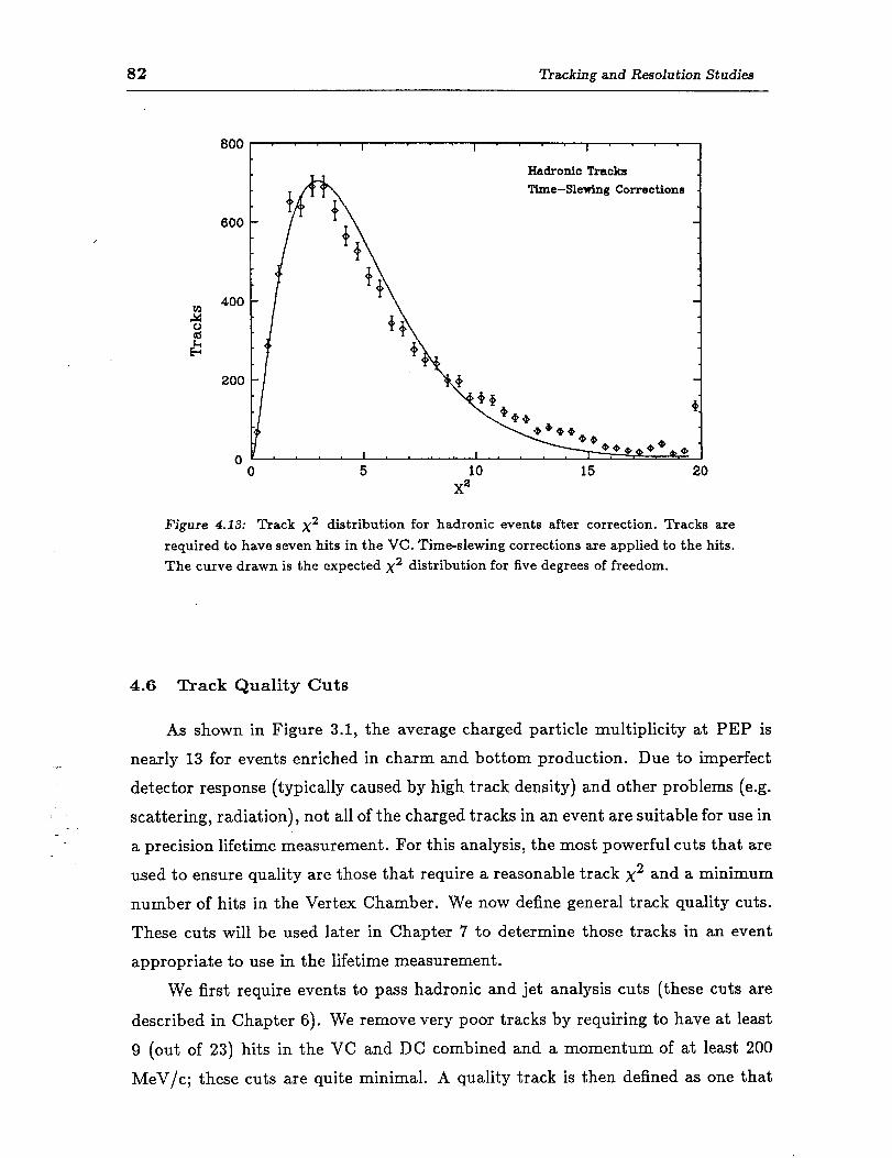
82 Tracking and Resolution Studies
Hadronic Tracks Time-Slewing Corrections
0 @a+/&*
0 5 10 15 20 X2
Figure 4.13: Track x 2 distribution for hadronic events after correction. Tracks are required to have seven hits in the VC. Time-slewing corrections are applied to the hits. The curve drawn is the expected x2 distribution for five degrees of freedom.
4.6 Track Quality Cuts
As shown in Figure 3.1, the average charged particle multiplicity at PEP is
nearly 13 for events enriched in charm and bottom production. Due to imperfect
detector response (typically caused by high track density) and other problems (e.g.
scattering, radiation), not all of the charged tracks in an event are suitable for use in
a precision lifetime measurement. For this analysis, the most powerful cuts that are
used to ensure quality are those that require a reasonable track x2 and a minimum
number of hits in the Vertex Chamber. We now define general track quality cuts.
These cuts will be used later in Chapter 7 to determine those tracks in an event
appropriate to use in the lifetime measurement.
We first require events to pass hadronic and jet analysis cuts (these cuts are
described in Chapter 6). We remove very poor tracks by requiring to have at least
9 (out of 23) hits in the VC and DC combined and a momentum of at least 200
MeV/c; these cuts are quite minimal. A quality track is then defined as one that
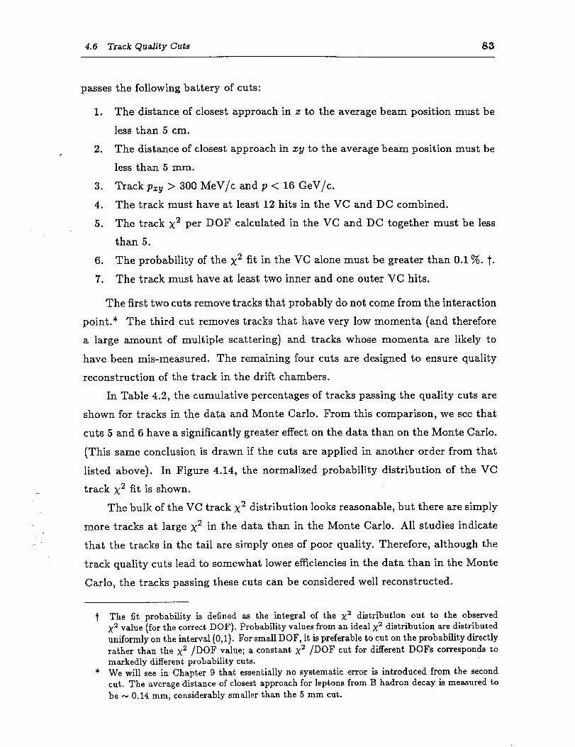
4.6 Track Quality Cuts 83
passes the following battery of cuts:
c
1.’ The distance of closest approach in x to the average beam position must be
less than 5 cm.
2. The distance of closest approach in zy to the average beam position must be
less than 5 mm.
3. Track pxY > 300 MeV/c and p < 16 GeV/c.
4. The track must have at least 12 hits in the VC and DC combined.
5. The track x2 per DOF calculated in the VC and DC together must be less
than 5.
6. The probability of the x2 fit in the VC alone must be greater than 0.1%. t.
7. The track must have at least two inner and one outer VC hits.
The first two cuts remove tracks that probably do not come from the interaction
point.* The third cut removes tracks that have very low momenta (and therefore
a large amount of multiple scattering) and tracks whose momenta are likely to
have been mis-measured. The remaining four cuts are designed to ensure quality
reconstruction of the track in the drift chambers.
In Table 4.2, the cumulative percentages of tracks passing the quality cuts are
shown for tracks in the data and Monte Carlo. From this comparison, we see that
cuts 5 and 6 have a significantly greater effect on the data than on the Monte Carlo.
(This same conclusion is drawn if the cuts are applied in another order from that
listed above). In Figure 4.14, the normalized probability distribution of the VC
track x2 fit is shown.
The bulk of the VC track x2 distribution looks reasonable, but there are simply
more tracks at large x2 in the data than in the Monte Carlo. All studies indicate
that the tracks in the tail are simply ones of poor quality. Therefore, although the
track quality cuts lead to somewhat lower efficiencies in the data than in the Monte
Carlo, the tracks passing these cuts can be considered well reconstructed.
t The fit probability is defined as the integral of the x 2 distribution out to the observed x2 value (for the correct DOF). Probability values from an ideal x 2 distribution are distributed uniformly on the interval (0,l). F or small DOF, it is preferable to cut on the probability directly rather than the x2 /DOF value; a constant x2 /DOE” cut for different DOFs corresponds to markedly different probability cuts.
* We will see in Chapter 9 that essentially no systematic error is introduced from the second cut. The average distance of closest approach for leptons from B hadron decay is measured to be - 0.14 mm, considerably smaller than the 5 mm cut.
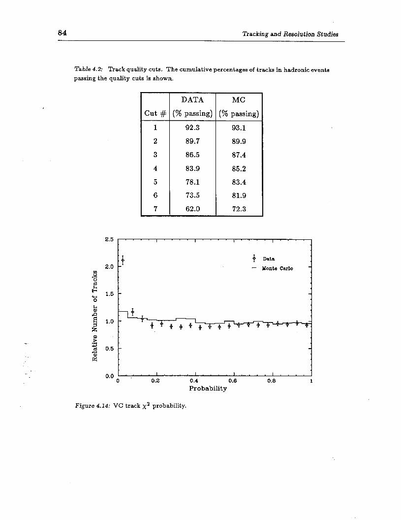
84 Tracking and Resolution Studies
Table 4.2; Track quality cuts. The cumulative percentages of tracks in hadronic events passing the quality cuts is shown.
DATA MC
Cut # (% passing) (% passing)
1 92.3 93.1
2 89.7 89.9
3 86.5 87.4
4 83.9 85.2
5 78.1 83.4
6 73.5 81.9
7 62.0 72.3
I ” “I’ “‘I”’ ‘ I’ ’ ”
0 Data
- Monte Carlo
Probability
Figure 4.14: VC track x2 probability.
Chapter 5
Lepton Identification
Electrons and muons can be distinguished from other charged particles by their
characteristic interactions with matter. Electrons lose energy upon entering matter
primarily by radiating photons through the bremsstrahlung process. These photons
produce electron-positron pairs which then can radiate more photons. This cascade
process continues, forming an electromagnetic shower of particles. The number
of particles increases with increasing depth into the material, but the average
particle energy decreases. The shower terminates when the particle energy reaches
a critical value below which energy loss through ionization dominates. The scale
of an electromagnetic shower in a given material is set by its radiation length X0,
defined as the mean free path length of electrons in the material.
The bremsstrahlung process of energy loss is suppressed for particles other
than the electron because of their larger masses. Hadrons lose energy in material
by interacting with the nuclei of the material via the strong interaction. This
process produces secondary particles (mostly pions and nucleons) which continue
to interact, resulting in a hadronic shower of particles. The scale of the hadronic
shower is set by the nuclear absorption length X of the material. For materials
with high 2 values, the nuclear absorption length is typically much larger than
the corresponding radiation length (e.g. in lead, X = 10.3 cm and X0 = 0.56
cm.) Electrons can therefore be expected to deposit almost all their energies in
an appropriately thick calorimeter made of such material, while hadrons of, the
same momenta will lose only a small fraction of their energy. This expectation is
86 Lepton Identification
the underlying principle behind electron identification in the Mark II calorimeter.
Hadrons sometimes resemble electrons because of shower fluctuations (especially in
the number of secondary ?y”‘s produced) or because of the presence of overlapping
charged tracks and photons.
Muons do not interact strongly and have masses too large to produce
bremsstrahlung photons. Muons lose energy in material primarily through uniform
ionization. Since the rate of energy loss for muons is much lower than that for
hadrons, they can be distinguished by their ability to penetrate material. The
Mark II muon system consists of steel absorber designed to stop most hadrons,
while allowing muons above a given momentum to penetrate.
The hardware details of the detector are outlined in Chapter 2. Here we discuss
how information from the detector is used to identify leptons. The algorithms
for electron and muon identification are presented. The identification efficiencies
are tabulated, along with the hadron mis-identification, punchthrough, and decay
probabilities. The probabilities for hadron mis-identification and punchthrough are
derived in part from a previous study of leptons in the Mark II detector [94]. These
probabilities have been checked with samples of known hadrons in the data [95].
In this chapter, and in the following one, tables are presented for given
quantities divided into bins of momentum (p) and transverse momentum (pt)
measured relative to the thrust axis. In these tables, the units for (p,pt) are GeV/c;
the (p,pt) values correspond to the low edge of each bin and the last bins contain
all overflows.
5.1 Electron Identification
5.1.1 Identification algorithm
Electrons are identified in the lead-liquid Argon (LA) calorimeter. The
calorimeter is described in Section 2.8. As shown in Figure 2.11, each calorimeter
module consists of 18 layers of lead strips that are ganged into six distinct readout
layers.
Identification is done by comparing the amount of energy a track deposits in
the calorimeter with the momentum of the track measured in the Drift Chamber.
Charged tracks in the DC are projected into the calorimeter and the energy ELA
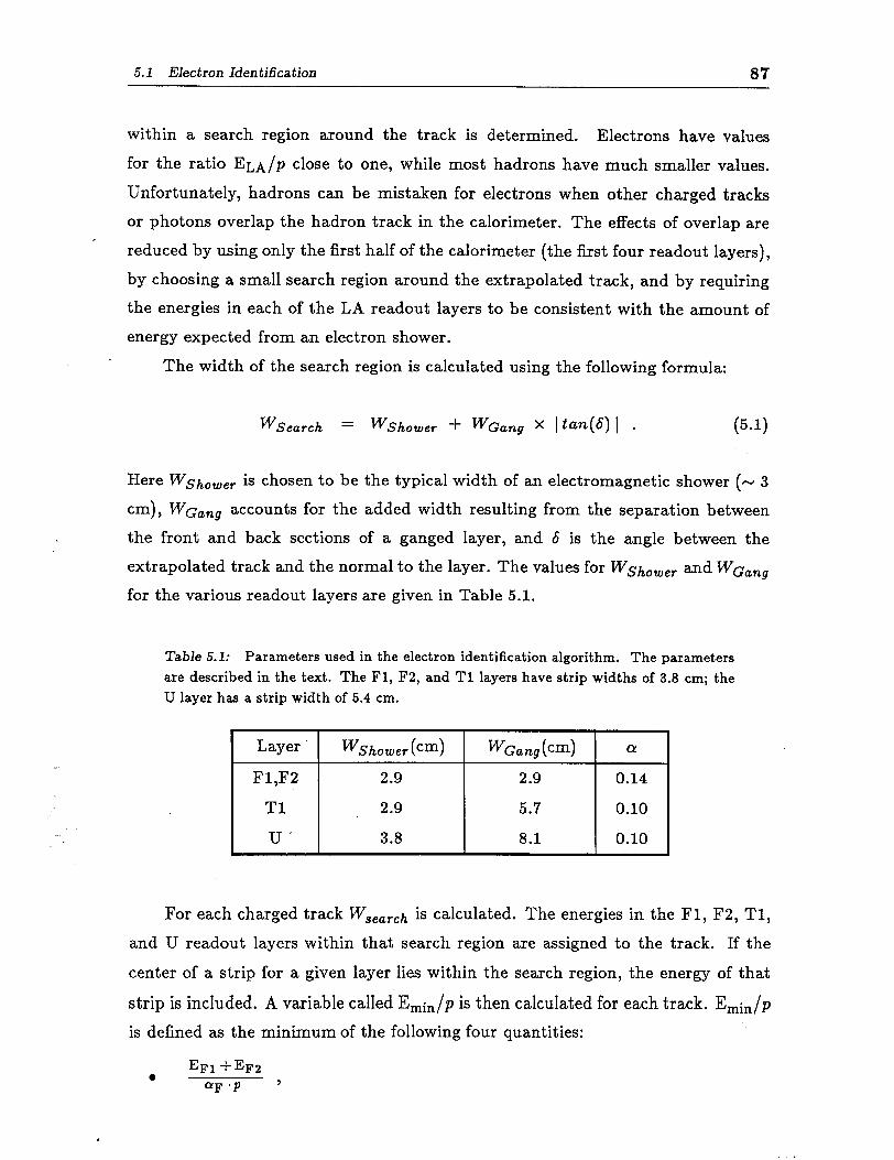
5.1 EIec tron Identification 87
within a search region around the track is determined. Electrons have values for the ratio ELA/P close to one, while most hadrons have much smaller values.
Unfortunately, hadrons can be mistaken for electrons when other charged tracks
or photons overlap the hadron track in the calorimeter. The effects of overlap are r
reduced by using only the first half of the calorimeter (the first four readout layers),
by choosing a small search region around the extrapolated track, and by requiring
the energies in each of the LA readout layers to be consistent with the amount of
energy expected from an electron shower.
The width of the search region is calculated using the following formula:
WSearch = WShoum + WGang x b-@> I . F-l)
Here WShower is chosen to be the typical width of an electromagnetic shower (- 3
cm), ~~~~~ accounts for the added width resulting from the separation between
the front and back sections of a ganged layer, and 6 is the angle between the
extrapolated track and the normal to the layer. The values for Wshower and ~~~~~
for the various readout layers are given in Table 5.1.
Table 5.1: Parameters used in the electron identification algorithm. The parameters are described in the text. The Fl, F2, and Tl layers have strip widths of 3.8 cm; the U layer has a strip width of 5.4 cm.
Layer WShower cm ( >
F&F2 2.9
Tl 2.9
U 3.8
WGang (cm) a
2.9 0.14
5.7 0.10
8.1 0.10
For each charged track Wsearch is calculated. The energies in the Fl, F2, Tl, and U readout layers within that search region are assigned to the track. If the
center of a strip for a given layer lies within the search region, the energy of that
strip is included. A variable called Emin/p is then calculated for each track. Emin/P is defined as the minimum of the following four quantities:
EF1 + EF2 0
aF ‘P 9
88 Lepton lden tifkation
ET1 0 -
‘?I”P ’
EU l -
“u -P , and
< EFl +EF2 +ET1 +EU 0
aFr’P .
Here p is the momentum of the track and EF~ is the energy in the Fl layer (similarly
for the F2,Tl, and U layers). The cx parameters account for the fact that showers
deposit only a fraction of their energy in each layer. The values for these parameters
are given in Table 5.1 (except for o!Fr which is 0.50 for p <4 GeV/c and 0.40 for
p >4 GeV/c). The values are chosen so that most electrons have values of Emin/P
greater than one.*
In Figure 5.1, the values of Emin/p f or samples of known electrons and pions
are shown. Clearly, as Emin/P increases, the probability for a pion track being
mis-identified as an electron decreases, but so too does the electron identification
efficiency.
In this analysis, electron candidates are defined as those tracks within the LA
fiducial volume satisfying:
E min/P > 1.1 ( Electron criterion ) . (5 2) .
5.12 Men tification efficiency
The cuts used to define the fiducial region of the LA calorimeter are discussed in
Section 2.8. This region covers - 65 % of the solid angle. The efficiency for detecting
electrons in collinear Bhabha events within the fiducial region is better than 98 %.
The identification efficiency for electrons with lower momenta is determined from
radiative Bhabha events and two-photon events of the type e+e- ---+ e+e-e+e-. These
two types of events together constitute a clean sample of electrons in the data
covering the entire momentum range of interest. The selection criteria for isolating
this sample of events and the method of determining the efficiency in an unbiased
way are described in Ref. 89.
The electron identification efficiency determined from this sample is given in
* Because of this (somewhat arbitrary) definition, Emin/p is typically larger than the simple ratio of the track energy divided by momentum.
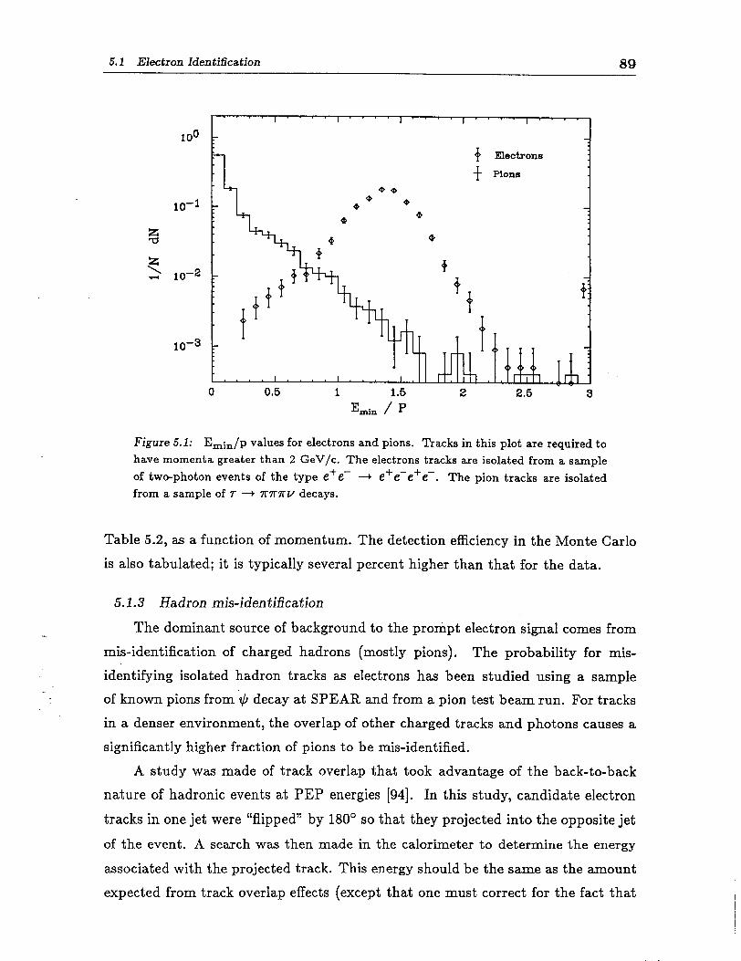
5.1 Electron Iden tifkation 89
--
Figure 5.1: Emin/p values for electrons and pions. Tracks in this plot are required to have momenta greater than 2 GeV/c. The electrons tracks are isolated from a sample of two-photon events of the type e+e- -+ e+e-e+e-. The pion tracks are isolated from a sample of 7 4 YMIT’/TV decays.
Table 5.2, as a function of momentum. The detection efficiency in the Monte Carlo
is also tabulated; it is typically several percent higher than that for the data.
5.1.3 Hadron mis-iden tifkation
The dominant source of background to the prompt electron signal comes from
mis-identification of charged hadrons (mostly pions). The probability for mis-
identifying isolated hadron tracks as electrons has been studied using a sample
of known pions from $J decay at SPEAR and from a pion test beam run. For tracks
in a denser environment, the overlap of other charged tracks and photons causes a
significantly higher fraction of pions to be mis-identified.
A study was made of track overlap that took advantage of the back-to-back
nature of hadronic events at PEP energies [94]. In this study, candidate electron
tracks in one jet were “flipped” by 180’ so that they projected into the opposite jet
of the event. A search was then made in the calorimeter to determine the energy
associated with the projected track. This energy should be the same as the amount
expected from track overlap effects (except that one must correct for the fact that
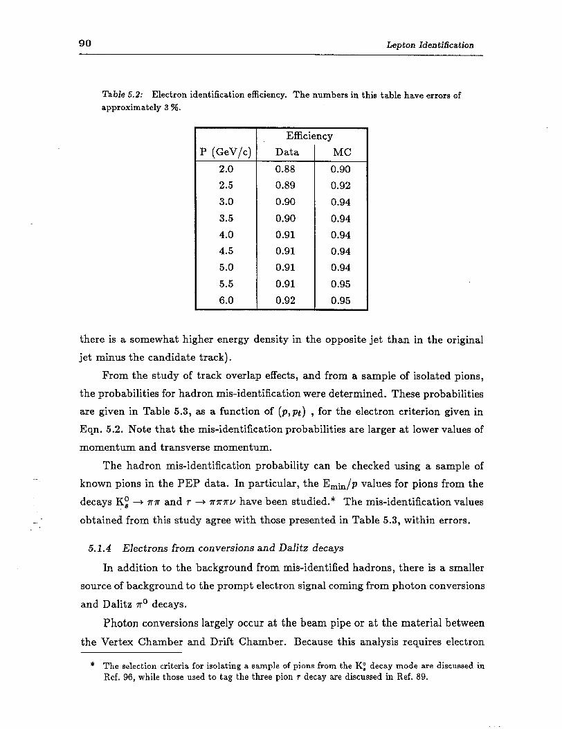
90 Lepton Identification
Table 5.2: Electron identification efficiency. The numbers in this table have errors of approximately 3 %.
P (GeV/c) Data MC 2.0 0.88 0.90 2.5 0.89 0.92 3.0 0.90 0.94
3.5 0.90 0.94 4.0 0.91 0.94 4.5 0.91 0.94 5.0 0.91 0.94 5.5 0.91 0.95 6.0 0.92 0.95
Efficiency
there is a somewhat higher energy density in the opposite jet than in the original
jet minus the candidate track).
From the study of track overlap effects, and from a sample of isolated pions,
the probabilities for hadron mis-identification were determined. These probabilities
are given in Table 5.3, as a function of (p,pt) , for the electron criterion given in
Eqn. 5.2. Note that the mis-identification probabilities are larger at lower values of
momentum and transverse momentum.
The hadron mis-identification probability can be checked using a sample of
known pions in the PEP data. In particular, the Emin/p values for pions from the
decays Kt + 7~ and r + ‘/T?T’ITL/ have been studied. * The mis-identification values
obtained from this study agree with those presented in Table 5.3, within errors.
5.1.4 Electrons from conversions and Dalitz decays
In addition to the background from mis-identified hadrons, there is a smaller
source of background to the prompt electron signal coming from photon conversions
and Dalitz no decays.
Photon conversions largely occur at the beam pipe or at the material between
the Vertex Chamber and Drift Chamber. Because this analysis requires electron
* The selection criteria for isolating a sample of pions from the Ki decay mode are discussed in Ref. 96, while those used to tag the three pion 7 decay are discussed in Ref. 89.
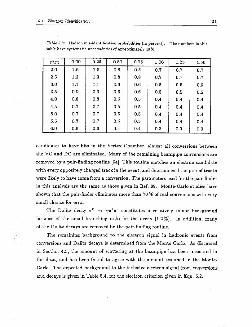
5.1 EIec tron Iden tifkation 91
Table 5.3: Hadron mis-identification probabilities (in percent). The numbers in this table have systematic uncertainties of approximately 40 %.
I P\Pt I
2.0 r 2.5
3.0
3.5
4.0
4.5
5.0
5.5
6.0
0.00 0.25 0.50 0.75 1.00 1.25 1.50
1.6 1.6 0.8 0.8 0.7 0.7 0.7
1.3 1.3 0.8 0.8 0.7 0.7 0.7
1.1 1.1 0.6 0.6 0.5 0.5 0.5
0.9 0.9 0.6 0.6 0.5 0.5 0.5
0.8 0.8 0.5 0.5 0.4 0.4 0.4
0.7 0.7 0.5 0.5 0.4 0.4 0.4
0.7 0.7 0.5 0.5 0.4 0.4 0.4
0.7 0.7 0.5 0.5 0.4 0.4 0.4
0.6 0.6 0.4 0.4 0.3 0.3 0.3
candidates to have hits in the Vertex Chamber, almost all conversions between
the VC and DC are eliminated. Many of the remaining beampipe conversions are
removed by a pair-finding routine [94]. This routine matches an electron candidate
with every oppositely charged track in the event, and determines if the pair of tracks
were likely to have come from a conversion. The parameters used for the pair-finder
in this analysis are the same as those given in Ref. 89. Monte-Carlo studies have
shown that the pair-finder eliminates more than 70 % of real conversions with very
small chance for error.
The Dalitz decay x0 -+ ye+e- constitutes a relatively minor background
because of the small branching ratio for the decay (1.2 %). In addition, many
of the Dalitz decays are removed by the pair-finding routine.
The remaining background to the electron signal in hadronic events from
conversions and Dalitz decays is determined from the Monte Carlo. As discussed
in Section 4.3, the amount of scattering at the beampipe has been measured in
the data, and has been found to agree with the amount assumed in the Monte-
Carlo. The expected background to the inclusive electron signal from conversions
and decays is given in Table 5.4, for the electron criterion given in Eqn. 5.2.
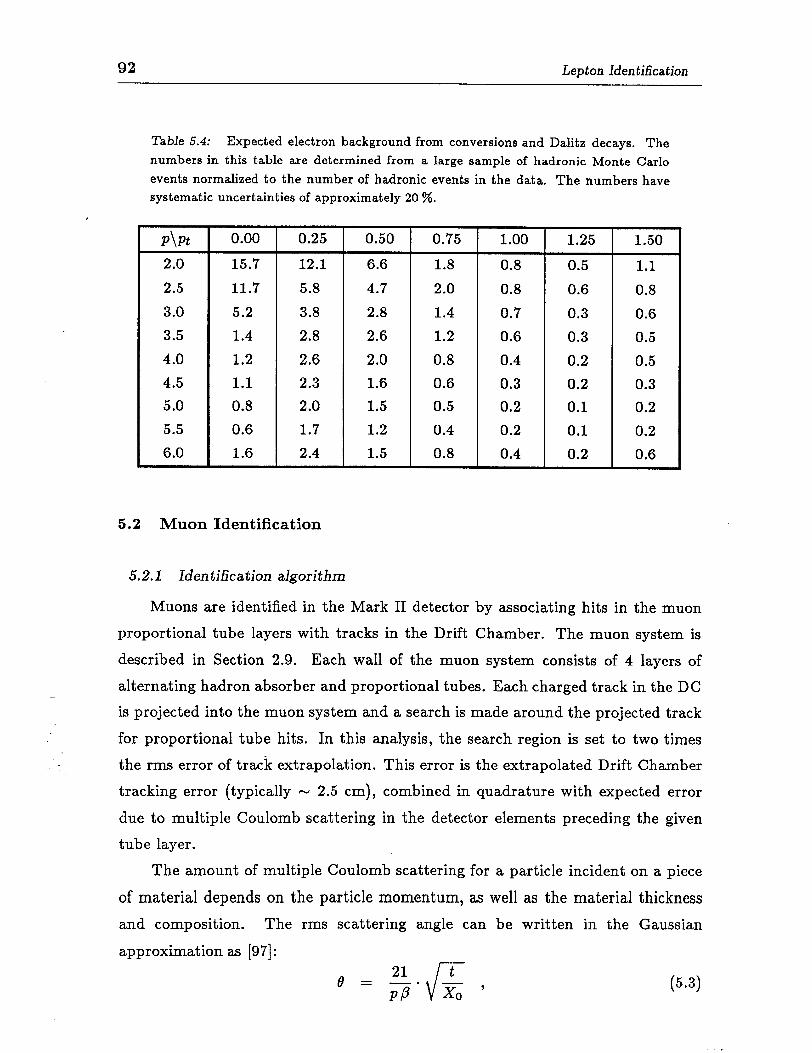
92 Lepton Identification
Table 5.4: Expected electron background from conversions and Dalitz decays. The numbers in this table are determined from a large sample of hadronic Monte Carlo events normalized to the number of hadronic events in the data. The numbers have systematic uncertainties of approximately 20 %.
P\Pt 0.00 0.25 0.50 0.75 1.00 1.25 1.50 2.0 15.7 12.1 6.6 1.8 0.8 0.5 1.1 2.5 11.7 5.8 4.7 2.0 0.8 0.6 0.8 3.0 5.2 3.8 2.8 1.4 0.7 0.3 0.6 3.5 1.4 2.8 2.6 1.2 0.6 0.3 0.5 4.0 1.2 2.6 2.0 0.8 0.4 0.2 0.5 4.5 1.1 2.3 1.6 0.6 0.3 0.2 0.3 5.0 0.8 2.0 1.5 0.5 0.2 0.1 0.2 5.5 0.6 1.7 1.2 0.4 0.2 0.1 0.2 6.0 1.6 2.4 1.5 0.8 0.4 0.2 0.6
5.2 Muon Identification
5.2.1 Identification algorithm
Muons are identified in the Mark II detector by associating hits in the muon
proportional tube layers with tracks in the Drift Chamber. The muon system is
described in Section 2.9. Each wall of the muon system consists of 4 layers of
alternating hadron absorber and proportional tubes. Each charged track in the DC
is projected into the muon system and a search is made around the projected track
for proportional tube hits. In this analysis, the search region is set to two times
the rms error of track extrapolation. This error is the extrapolated Drift Chamber
tracking error (typically - 2.5 cm), combined in quadrature with expected error
due to multiple Coulomb scattering in the detector elements preceding the given
tube layer.
The amount of multiple Coulomb scattering for a particle incident on a piece
of material depends on the particle momentum, as well as the material thickness and composition. The rms scattering angle can be written in the Gaussian
approximation as [97]:
(5 3) .
5.2 Muon Iden tiika tion 93
where p is the momentum (in MeV/c) and ,B the velocity of the incident particle.
The material thickness and radiation length are given by t and X0, respectively.
In the Mark II , the detector elements preceding the proportional tubes are the
magnet coil (1.4 X0), the LA calorimeter (14.4 X0), and hadron absorbers (13.0 r
Xo/layer). The scattering effects of each element are independent, therefore their
contributions can be added in quadrature. In a given layer of the muon system, the
mean-squared position error projected in one dimension* due to multiple scattering
can be expressed as [98]:
2 fTsr: = ; c t9; l ($ + t& + df ) ,
i
(5 4) .
where &; is the distance following the element i to the given layer, and t; and 8i are
the thickness and rms scattering angle of the element i, respectively. The typical
position error for a 2 GeV muon due to multiple scattering is 5 cm at the first layer
of the muon system and 10 cm at the fourth layer.
For each track, a variable MUSTAT is formed. This variable corresponds to the
bit pattern of the muon system layers having hits associated with the given track.
(For example, a track with associated hits in the first three layers has MUSTAT=7.)
In this analysis, muon candidates are defined as those tracks within the muon system
fiducial region (discussed below) satisfying:
MUSTAT = 15 ( Muon criterion) , (5 5) .
i.e. having associated hits in all four of the muon layers.
5.2.2 .ldentification efficiency
Since muons are required to have hits in all four proportional tube layers, the
fiducial region of the muon system is defined by the acceptance of the outermost
tube layer in each wall. These layers cover - 45 % of the solid angle. In addition,
muon candidates are required to have sufficient momenta to penetrate to the fourth
layer. For tracks at normal incidence to the absorber planes, this criterion effectively
imposes a 1.8 GeV/c momentum cut.
* In a given layer, the proportional tubes measure only one coordinate.
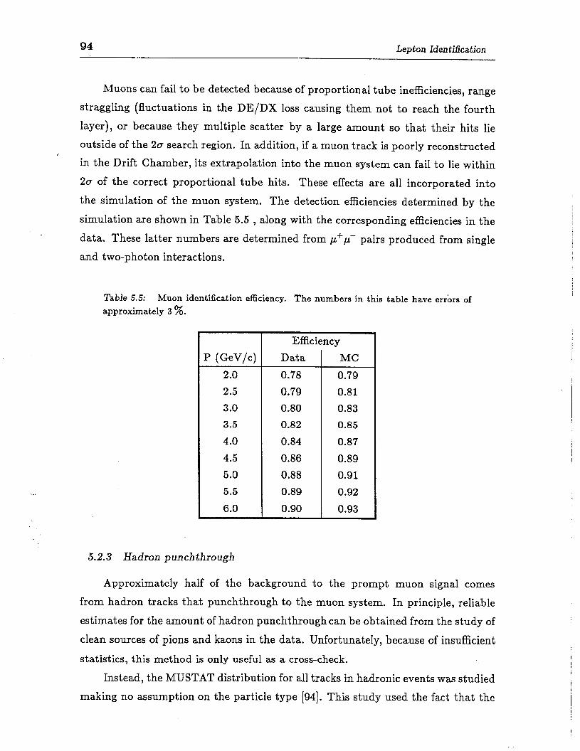
94 Lep t on Iden tifkation
Muons can fail to be detected because of proportional tube inefficiencies, range
straggling (fluctuations in the DE/DX loss causing them not to reach the fourth
layer), or because they multiple scatter by a large amount so that their hits lie
outside of the 20 search region. In addition, if a muon track is poorly reconstructed
in the Drift Chamber, its extrapolation into the muon system can fail to lie within
20 of the correct proportional tube hits. These effects are all incorporated into
the simulation of the muon system. The detection efficiencies determined by the
simulation are shown in Table 5.5 , along with the corresponding efficiencies in the
data. These latter numbers are determined from ,?.&- pairs produced from single
and two-photon interactions.
Table 5.5: Muon identification efficiency. The numbers in this table have err&s of approximately 3 %.
P (GeV/c) 2.0 2.5 3.0 3.5 4.0 4.5 5.0 5.5 6.0
Efficiency Data MC 0.78 0.79 0.79 0.81 0.80 0.83 0.82 0.85 0.84 0.87 0.86 0.89 0.88 0.91 0.89 0.92 0.90 0.93
5.2.3 Hadron punchthrough
Approximately half of the background to the prompt muon signal comes
from hadron tracks that punchthrough to the muon system. In principle, reliable
estimates for the amount of hadron punchthrough can be obtained from the study of
clean sources of pions and kaons in the data. Unfortunately, because of insufficient
statistics, this method is only useful as a cross-check.
Instead, the MUSTAT distribution for all tracks in hadronic events was studied
making no assumption on the particle type [94]. Th is study used the fact that the
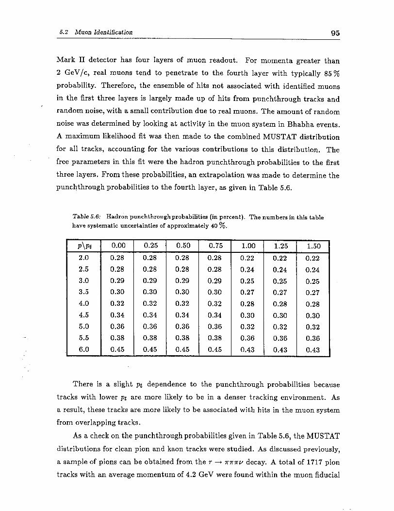
5.2 Muon Iden tidication 95
Mark II detector has four layers of muon readout. For momenta greater than
2 GeV/c, real muons tend to penetrate to the fourth layer with typically 85 %
probability. Therefore, the ensemble of hits not associated with identified muons
in the first three layers is largely made up of hits from punchthrough tracks and <
random noise, with a small contribution due to real muons. The amount of random
noise was determined by looking at activity in the muon system in Bhabha events.
A maximum likelihood fit was then made to the combined MUSTAT distribution
for all tracks, accounting for the various contributions to this distribution. The
free parameters in this fit were the hadron punchthrough probabilities to the first
three layers. From these probabilities, an extrapolation was made to determine the
punchthrough probabilities to the fourth layer, as given in Table 5.6.
Table 5.6: Hadron punchthroughprobabilities (in percent). The numbers in this table have systematic uncertainties of approximately 40 %.
I Apt 2.0 2.5 3.0 3.5 4.0 4.5 5.0
I 5.5
I 6.0
0.00 0.25 0.50 0.75 1.00 1.25 1.50 0.28 0.28 0.28 0.28 0.22 0.22 0.22 0.28 0.28 0.28 0.28 0.24 0.24 0.24 0.29 0.29 0.29 0.29 0.25 0.25 0.25 0.30 0.30 0.30 0.30 0.27 0.27 0.27 0.32 0.32 0.32 0.32 0.28 0.28 0.28 0.34 0.34 0.34 0.34 0.30 0.30 0.30 0.36 0.36 0.36 0.36 0.32 0.32 0.32 0.38 0.38 0.38 0.38 0.36 0.36 0.36 0.45 0.45 0.45 0.45 0.43 0.43 0.43
There is a slight pt dependence to the punchthrough probabilities because
tracks with lower pt are more likely to be in a denser tracking environment. As
a result, these tracks are more likely to be associated with hits in the muon system
from overlapping tracks.
As a check on the punchthrough probabilities given in Table 5.6, the MUSTAT
distributions for clean pion and kaon tracks were studied. As discussed previously,
a sample of pions can be obtained from the r -+ 7~7~ decay. A total of 1717 pion
tracks with an average momentum of 4.2 GeV were found within the muon fiducial
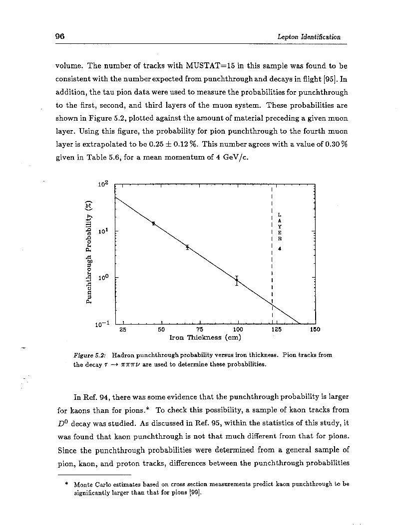
96 Lepton Identification
volume. The number of tracks with MUSTAT= in this sample was found to be
consistent with the number expected from punchthrough and decays in flight [95]. In
addition, the tau pion data were used to measure the probabilities for punchthrough
< to the first, second, and third layers of the muon system. These probabilities are
shown in Figure 5.2, plotted against the amount of material preceding a given muon
layer. Using this figure, the probability for pion punchthrough to the fourth muon
layer is extrapolated to be 0.25 -+ 0.12 %. This number agrees with a value of 0.30 %
given in Table 5.6, for a mean momentum of 4 GeV/c.
50 75 100 125 150 Iron Thickness (cm)
Figure 5.2: Hadron punchthrough probability versus iron thickness. Pion tracks from the decay T -+ ‘/T’/T’/Tv are used to determine these probabilities.
In Ref. 94, there was some evidence that the punchthroughprobability is larger
for kaons than for pions. * To check this possibility, a sample of kaon tracks from
Do decay was studied. As discussed in Ref. 95, within the statistics of this study, it
was found that kaon punchthrough is not that much different from that for pions.
Since the punchthrough probabilities were determined from a general sample of pion, kaon, and proton tracks, differences between the punchthrough probabilities
* Monte Carlo estimates based on cross section measurements predict kaon punchthrough to be significantly larger than that for pions [99].
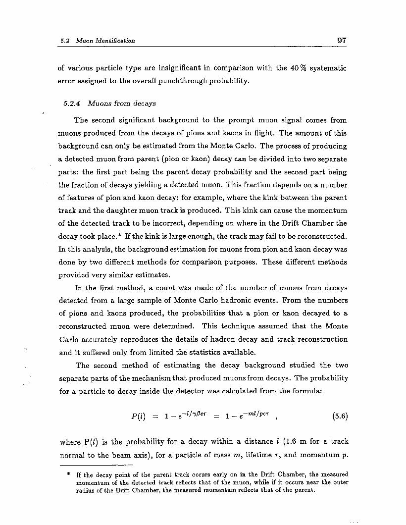
5.2 Muon Identification 97
of various particle type are insignificant in comparison with the 40% systematic
error assigned to the overall punchthrough probability.
52.4 Muons from decays
The second significant background to the prompt muon signal comes from
muons produced from the decays of pions and kaons in flight. The amount of this
background can only be estimated from the Monte Carlo. The process of producing
a detected muon from parent (pion or kaon) decay can be divided into two separate
parts: the first part being the parent decay probability and the second part being
the fraction of decays yielding a detected muon. This fraction depends on a number
of features of pion and kaon decay: for example, where the kink between the parent
track and the daughter muon track is produced. This kink can cause the momentum
of the detected track to be incorrect, depending on where in the Drift Chamber the
decay took place. * If the kink is large enough, the track may fail to be reconstructed.
In this analysis, the background estimation for muons from pion and kaon decay was
done by two different methods for comparison purposes. These different methods
provided very similar estimates.
In the first method, a count was made of the number of muons from decays
detected from a large sample of Monte Carlo hadronic events. From the numbers
of pions and kaons produced, the probabilities that a pion or kaon decayed to a
reconstructed muon were determined. This technique assumed that the Monte
Carlo accurately reproduces the details of hadron decay and track reconstruction
and it suffered only from limited the statistics available.
The second method of estimating the decay background studied the two
separate parts of the-mechanism that produced muons from decays. The probability
for a particle to decay inside the detector was calculated from the formula:
P(l) = I- e--l17PCr = I_ e-ml/per , (54
where P(1) is the probability for a decay within a distance I (1.6 m for a track
normal to the beam axis), for a particle of mass m, lifetime 7, and momentum p.
* If the decay point of the parent track occurs early on in the Drift Chamber, the measured momentum of the detected track reflects that of the muon, while if it occurs near the outer radius of the Drift Chamber, the measured momentum reflects that of the parent.
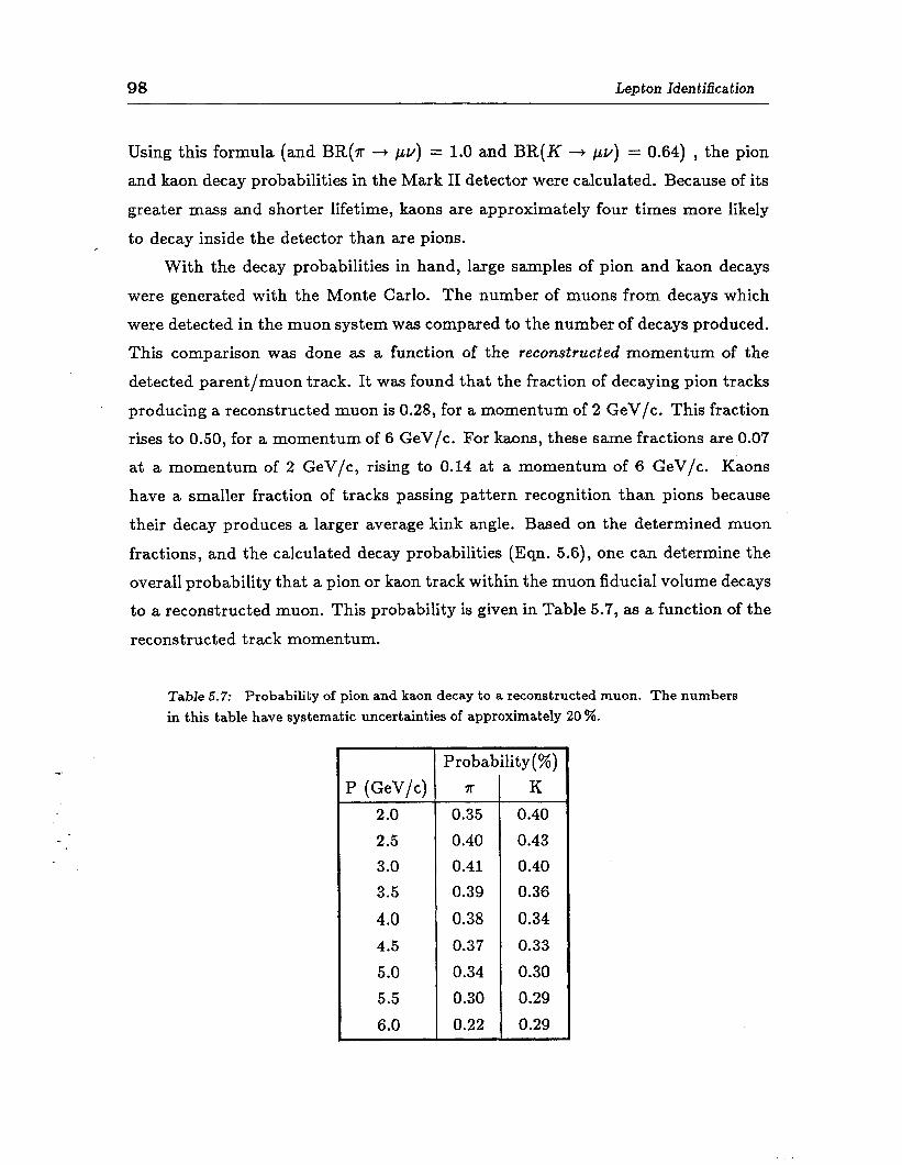
98 Lepton Identification
Using this formula (and BR(x --$ PV) = 1.0 and BR(K + pv) = 0.64) , the pion
and kaon decay probabilities in the Mark II detector were calculated. Because of its
greater mass and shorter lifetime, kaons are approximately four times more likely
to decay inside the detector than are pions. r: With the decay probabilities in hand, large samples of pion and kaon decays
were generated with the Monte Carlo. The number of muons from decays which
were detected in the muon system was compared to the number of decays produced.
This comparison was done as a function of the reconstructed momentum of the
detected parent/muon track. It was found that the fraction of decaying pion tracks
producing a reconstructed muon is 0.28, for a momentum of 2 GeV/c. This fraction
rises to 0.50, for a momentum of 6 GeV/c. For kaons, these same fractions are 0.07 at a momentum of 2 GeV/c, rising to 0.14 at a momentum of 6 GeV/c. Kaons
have a smaller fraction of tracks passing pattern recognition than pions because
their decay produces a larger average kink angle. Based on the determined muon
fractions, and the calculated decay probabilities (Eqn. 5.6), one can determine the
overall probability that a pion or kaon track within the muon fiducial volume decays
to a reconstructed muon. This probability is given in Table 5.7, as a function of the
reconstructed track momentum.
Table 5.7: Probability of pion and kaon decay to a reconstructed muon. The numbers
in this table have systematic uncertainties of approximately 20 %.
Probability( %) P (GeV/c) ?r K
2.0 0.35 0.40 2.5 0.40 0.43 3.0 0.41 0.40 3.5 0.39 0.36 4.0 0.38 0.34 4.5 0.37 0.33 5.0 0.34 0.30 5.5 0.30 0.29 6.0 0.22 0.29