Embed Size (px)
Citation preview

Measurement of Open Charm and DoubleOpen Charm Production Cross Sections andRatios in pp Collisions at
√s = 2.76 TeV with
the LHCb Experiment
Master Thesiszur
Erlangung des akademischen Grades Master of Science (MSc)
Vorgelegt derMathematisch-Naturwissenschaftlichen Fakultat
derUniversitat Zurich
VonEnzio Crivelli
ausSolothurn, Schweiz
Aufsicht:Prof. Dr. Ulrich Straumann (Vorsitz)
Dr. Katharina MullerDr. Albert Bursche
Zurich15. Juni 2016


Abstract
In proton-proton collisions, mechanisms other than gluon-gluon fusion can contributeto double charm production. One possible additional source is double parton scattering(DPS). The theory of Quantum Chromodynamics cannot precisely predict DPS produc-tion cross sections, since simplifications have to be used. Double open charm productioncross sections in proton-proton collisions at LHCb have been measured so far at a centre ofmass energy of
√s = 7 TeV (see [2], [3]). These provide valuable input for the theoretical
understanding of DPS. In this work such double open charm production cross sections aremeasured at LHCb at
√s = 2.76 TeV using D0 and D+ mesons in the final state.

Acknowledgement
It is almost impossible for one person alone to contribute to one of the four major exper-iments at the LHC at CERN, like LHCb. The LHC with its experiments is simply waytoo large and complicated, that a few people are able to develop, operate and conduct thefundamental research in particle physics all by themselves. In order to work efficiently andsuccessfully, the organization, communication and exchange of knowledge within a groupof several hundreds or thousands of people is of utmost importance. It was impressive tosee how much work people are able to manage, while still offering the time to answer myquestions. This thrilling working atmosphere results in the exploitment of the personalcapability in order to be able to provide at least a halfway decent amount of support forthe groups, in which I was involved. Everyone I had the pleasure to work with deservesmy respect for their unreservedly way of communication, support and cooperative work.Otherwise this work would not have been possible.
Primarily my thanks goes to my supervisors, Prof. Dr. Ulrich Straumann for giving methe chance to develop my master thesis in the LHCb group at CERN and for organizingand managing the group in a way that keeps the balance of challenge, social interactionand (self-)responsibility, and Dr. Katharina Muller as well as Dr. Albert Bursche for manyinteresting and fruitful discussions and their great support during my work. Secondly, Ithank various members of the LHCb group, which provided useful help in different areasof the analysis, talks and discussions: J. Anderson, I. Belyaev, R. Bernet, N. Chiapolini,M. De Cian, C. Elsasser, F. Lionetto, P. Lowdon, O. Steinkamp, M. Tresch, A. Weiden (inalphabetical order).

Contents
1 Introduction 6
2 Theory 72.1 The Standard Model of Particle Physics (SM) . . . . . . . . . . . . . . . . 72.2 The Double Parton Scattering (DPS) Model . . . . . . . . . . . . . . . . . 17
3 Foundations: LHC Collider, LHCb Detector and Key Concepts for the Analysis 193.1 The LHC at CERN . . . . . . . . . . . . . . . . . . . . . . . . . . . . . . . 19
3.1.1 The LHCb Detector . . . . . . . . . . . . . . . . . . . . . . . . . . 223.1.2 Key Concepts for the Analysis . . . . . . . . . . . . . . . . . . . . . 25
4 Cross Section Determination 344.1 Analysis Strategy . . . . . . . . . . . . . . . . . . . . . . . . . . . . . . . . 354.2 Event Selection and Background Determination . . . . . . . . . . . . . . . 37
4.2.1 Event Selection . . . . . . . . . . . . . . . . . . . . . . . . . . . . . 374.2.2 Pile-Up and Feed-Down . . . . . . . . . . . . . . . . . . . . . . . . 42
4.3 Selected Candidates . . . . . . . . . . . . . . . . . . . . . . . . . . . . . . . 454.4 Invariant Mass Fits . . . . . . . . . . . . . . . . . . . . . . . . . . . . . . . 494.5 Efficiency Corrected Yields . . . . . . . . . . . . . . . . . . . . . . . . . . . 674.6 Efficiency . . . . . . . . . . . . . . . . . . . . . . . . . . . . . . . . . . . . 71
4.6.1 Global Event Cut Efficiency . . . . . . . . . . . . . . . . . . . . . . 864.7 Integrated Luminosity . . . . . . . . . . . . . . . . . . . . . . . . . . . . . 914.8 Branching Ratios . . . . . . . . . . . . . . . . . . . . . . . . . . . . . . . . 914.9 Systematic Uncertainties . . . . . . . . . . . . . . . . . . . . . . . . . . . . 92
5 Results 99
6 Conclusion and Outlook 104
A Invariant Mass Fit Parameters 105
B GEC Efficiency Fit Parameters 110
C Analysis for additionally applied (pT [GeV], y) > (4, 2.25) 113C.1 Results . . . . . . . . . . . . . . . . . . . . . . . . . . . . . . . . . . . . . . 113C.2 Systematic Uncertainties . . . . . . . . . . . . . . . . . . . . . . . . . . . . 117
5
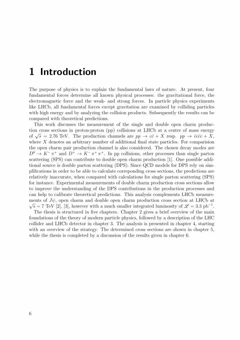
1 Introduction
The purpose of physics is to explain the fundamental laws of nature. At present, fourfundamental forces determine all known physical processes: the gravitational force, theelectromagnetic force and the weak- and strong forces. In particle physics experimentslike LHCb, all fundamental forces except gravitation are examined by colliding particleswith high energy and by analyzing the collision products. Subsequently the results can becompared with theoretical predictions.
This work discusses the measurement of the single and double open charm produc-tion cross sections in proton-proton (pp) collisions at LHCb at a center of mass energyof√s = 2.76 TeV. The production channels are pp → cc + X resp. pp → cccc + X,
where X denotes an arbitrary number of additional final state particles. For comparisionthe open charm pair production channel is also considered. The chosen decay modes areD0 → K− π+ and D+ → K− π+ π+. In pp collisions, other processes than single partonscattering (SPS) can contribute to double open charm production [1]. One possible addi-tional source is double parton scattering (DPS). Since QCD models for DPS rely on sim-plifications in order to be able to calculate correponding cross sections, the predictions arerelatively inaccurate, when compared with calculations for single parton scattering (SPS)for instance. Experimental measurements of double charm production cross sections allowto improve the understanding of the DPS contributions in the production processes andcan help to calibrate theoretical predictions. This analysis complements LHCb measure-ments of Jψ, open charm and double open charm production cross section at LHCb at√s = 7 TeV [2], [3], however with a much smaller integrated luminosity of L = 3.3 pb−1.The thesis is structured in five chapters. Chapter 2 gives a brief overview of the main
foundations of the theory of modern particle physics, followed by a description of the LHCcollider and LHCb detector in chapter 3. The analysis is presented in chapter 4, startingwith an overview of the strategy. The determined cross sections are shown in chapter 5,while the thesis is completed by a discussion of the results given in chapter 6.
6

2 Theory
The standard model of particle physics (SM) is able to explain most the observed phe-nomena in particle physics. It describes the elementary particles and their fundamentalinteractions by three of four fundamental forces of nature, being the electromagnetic forceand the weak- and strong forces, but not gravitation. Known shortcomings lie in the lackof explanation for dark matter and dark energy as well as the abundance of matter overantimatter.
This chapter follows standard textbooks [4], [5], [6]. Due to the extension and complexityof the SM it is only intended to give a brief overview of the main foundations of themodern understanding of fundamental particle physics. This includes the fundamentaland composite particles with their interactions encountered at particle colliders like theLHC in chapter 2.1 and the DPS model explained in chapter 2.2.
2.1 The Standard Model of Particle Physics (SM)
The SM consists of fundamental particles, i.e particles that are assumed to be point-likeand have consequently no inner structure, classified according to their interaction ability(see Tab. 2.1 and Tab. 2.2).
Fundamental ParticlesThese are the electrically neutral gauge bosons γ, Z, g, H, the charged gauge bosons W±,the charged leptons e±, µ±, τ±, the electrically neutral leptons νe, νµ, ντ , called neutrinos,and the quarks u, d, c, s, t, b. They can be split by the quantum number (QN) of spin sinto two groups, the bosons (s 1) (including the higgs (s 0)) and fermions (s 1/2).
• FermionsEach fermion f has an antiparticle state with the same qualities with the exceptionof an opposite charge QN qe, denoted by a bar (e.g. u). The fermions can be splitfurther by the QN of isospin I into doublets leading to three families. There are twogroups of fermions, called leptons l and quarks q.
The leptons l consist of the charged electron, muon and tau with qe = −1, of whichonly the electron is stable, and the corresponding electrically neutral neutrinos. Theseneutrinos usually escape detection in most particle collider experiments, since theyexclusively interact by the weak force resulting in very small cross sections.
The quarks q exist in six flavours, up (u), down (d), charm (c), strange (s), top(t) and bottom (b) and have a non-integer charge of qe = +2/3 resp. qe = −1/3.
7
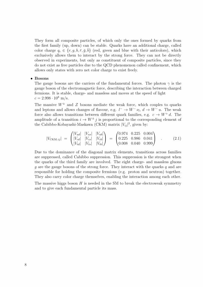
They form all composite particles, of which only the ones formed by quarks fromthe first family (up, down) can be stable. Quarks have an additional charge, calledcolor charge qc ∈ {r, g, b, r, g, b} (red, green and blue with their anticolors), whichexclusively allows them to interact by the strong force. They can not be directlyobserved in experiments, but only as constituent of composite particles, since theydo not exist as free particles due to the QCD phenomenon called confinement, whichallows only states with zero net color charge to exist freely.
• BosonsThe gauge bosons are the carriers of the fundamental forces. The photon γ is thegauge boson of the electromagnetic force, describing the interaction between chargedfermions. It is stable, charge- and massless and moves at the speed of lightc = 2.998 · 108 m/s.
The massive W± and Z bosons mediate the weak force, which couples to quarksand leptons and allows changes of flavour, e.g. l− → W− νl, d → W− u. The weakforce also allows transitions between different quark families, e.g. c → W+ d. Theamplitude of a transition i → W± j is proportional to the corresponding element ofthe Cabibbo-Kobayashi-Maskawa (CKM) matrix |Vij|2, given by:
|VCKM; ij| =
|Vud| |Vus| |Vub||Vcd| |Vcs| |Vcb||Vtd| |Vts| |Vtb|
=
0.974 0.225 0.0040.225 0.986 0.0410.008 0.040 0.999
. (2.1)
Due to the dominance of the diagonal matrix elements, transitions across familiesare suppressed, called Cabibbo suppression. This suppression is the strongest whenthe quarks of the third family are involved. The eight charge- and massless gluonsg are the gauge bosons of the strong force. They interact with the quarks q and areresponsible for holding the composite fermions (e.g. proton and neutron) together.They also carry color charge themselves, enabling the interaction among each other.
The massive higgs boson H is needed in the SM to break the electroweak symmetryand to give each fundamental particle its mass.
8

Quantity 1st family 2nd family 3rd family
Quarks
up (u) charm (c) top (t)
q +2/3 +2/3 +2/3
M0 [MeV/c2] ≈ 2− 3.5 ≈ 1.27 · 103 ≈ 172 · 103
s 1/2 1/2 1/2
down (d) strange (s) bottom (b)
q −1/3 −1/3 −1/3
M0 [MeV/c2] ≈ 4− 5.5 ≈ 101 ≈ 4.67 · 103
s 1/2 1/2 1/2
Leptons
electron (e−) muon (µ−) tau (τ−)
q −1 −1 −1
M0 [MeV/c2] = 0.511 = 105 = 1780
s 1/2 1/2 1/2
electron neutrino (νe) muon neutrino (νµ) tau neutrino (ντ )
q 0 0 0
M0 < 2 eV/c2 95% CL < 17 keV/c2 95% CL < 1.23 MeV/c2 95% CL
s 1/2 1/2 1/2
Table 2.1: Overview of the fermions in the Standard Model (SM) [7]. For each fermion f ananti-particle state exists, denoted by f . Since such anti-particle states have thesame qualities as the corresponding fermions, with the exception of the oppositecharge-like QN, they are not listed in the table.
9

Qu
antity
GaugeBoso
ns
ph
oton(γ
)W
±,Z
boso
ns
glu
on
(g;8
colorch
arges)H
iggs(H
)
q0
±1
(W±
),0
(Z)
00
M0
[GeV/c
2]0
=80.4
(W±
),91.2
(Z)
0≈
126
s1
11
1
Intera
ctionT
yp
eelectrom
agn
eticw
eak
strong
higgs
mech
anism
Tab
le2.2:
Overv
iewof
the
boson
sw
ithth
eiraccom
pan
yin
gin
teractionin
the
SM
[7].
10

The quarks form composite particles, called hadrons, whose properties are largely de-termined by their valence quarks. The gluons holding such a hadron together constantlyproduce and annihilate quark-antiquark pairs qq (sea quarks) due to their self interactionby the strong force.
Composite ParticlesAccording to the number of valence quarks, hadrons can be structured into two groups:the baryons containing three quarks and the mesons consisting of a quark-antiquark pair.
• BaryonsThe most common hadrons are the proton p and neutron n, whose valence quarkcontent is p = uud and n = udd. They are the components of the atomic nucleilisted in the periodic system of elements. All baryons, with the possible exception ofthe proton, are unstable. For example, when not bound in a nuclei, a free neutrondecays into a proton, electron and electron neutrino with a lifetime of about 900 s.This radioactive β-decay was the first experimentally observed process involving theweak force. Whether the proton can be considered as stable or not is the subject ofcurrent experimental research. Since no proton decay is so far observed, lower limitsof the lifetime with 90% confidence limit of about 1040 s have been determined [7].Due to such extremely long lifetime expectations, the proton is considered as stablein this work.
• MesonsNo meson is observed to be stable. The most common ones, the kaons (K) and pions(π), decay with a lifetime of about 10−8 s [7]. Such long lifetimes allow for theirmeasurement as the traverse through the LHCb detector. They are of particularinterest in this work, since the investigated D0 and D+ mesons decay into K and π.
The lightest mesons involving one charm quark, D0 = c u, D+ = c d and D+s = c s
with their antiparticles D0 = c u, D− = c d and D−s = c s are called D mesons or opencharm mesons, due to the not specified quark accompanying the charm. In hadron colliderexperiments like the LHC experiment, they are produced by the interaction of quarks,which is described by the theory of Quantum Chromodynamics (QCD).
QCD production processes of D mesonsIn this non-abelian gauge theory the eight gluons can interact among themselves, leadingto complicated processes. The force behaves differently depending on the energy scale withthe two extremes of confinement and asymptotic freedom. Since the QCD describes thestrong force, a perturbative expansion ansatz is not always feasible. Although numericaland analytical methods to approximate QCD such as lattice QCD exist, perturbative QCDcan only be carried out for high energies. The theory offers some interesting characteristics.
11
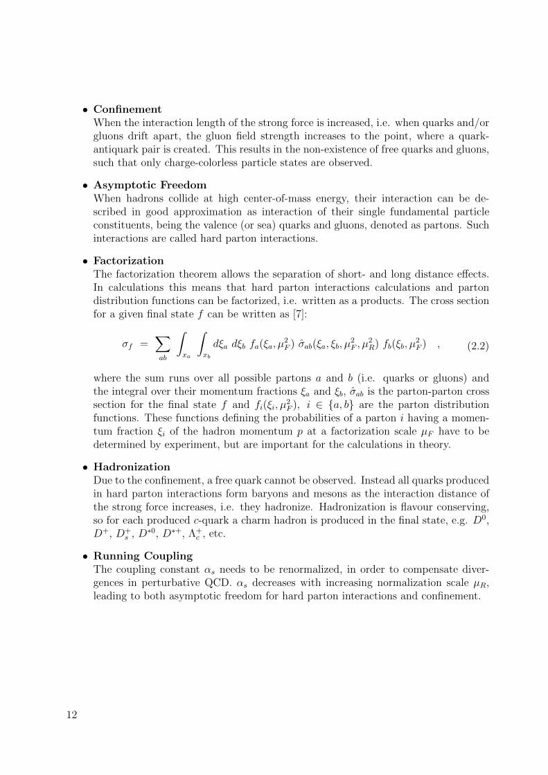
• ConfinementWhen the interaction length of the strong force is increased, i.e. when quarks and/orgluons drift apart, the gluon field strength increases to the point, where a quark-antiquark pair is created. This results in the non-existence of free quarks and gluons,such that only charge-colorless particle states are observed.
• Asymptotic FreedomWhen hadrons collide at high center-of-mass energy, their interaction can be de-scribed in good approximation as interaction of their single fundamental particleconstituents, being the valence (or sea) quarks and gluons, denoted as partons. Suchinteractions are called hard parton interactions.
• FactorizationThe factorization theorem allows the separation of short- and long distance effects.In calculations this means that hard parton interactions calculations and partondistribution functions can be factorized, i.e. written as a products. The cross sectionfor a given final state f can be written as [7]:
σf =∑ab
∫xa
∫xb
dξa dξb fa(ξa, µ2F ) σab(ξa, ξb, µ
2F , µ
2R) fb(ξb, µ
2F ) , (2.2)
where the sum runs over all possible partons a and b (i.e. quarks or gluons) andthe integral over their momentum fractions ξa and ξb, σab is the parton-parton crosssection for the final state f and fi(ξi, µ
2F ), i ∈ {a, b} are the parton distribution
functions. These functions defining the probabilities of a parton i having a momen-tum fraction ξi of the hadron momentum p at a factorization scale µF have to bedetermined by experiment, but are important for the calculations in theory.
• HadronizationDue to the confinement, a free quark cannot be observed. Instead all quarks producedin hard parton interactions form baryons and mesons as the interaction distance ofthe strong force increases, i.e. they hadronize. Hadronization is flavour conserving,so for each produced c-quark a charm hadron is produced in the final state, e.g. D0,D+, D+
s , D∗0, D∗+, Λ+c , etc.
• Running CouplingThe coupling constant αs needs to be renormalized, in order to compensate diver-gences in perturbative QCD. αs decreases with increasing normalization scale µR,leading to both asymptotic freedom for hard parton interactions and confinement.
12

If the D mesons are produced at high transverse momentum, the QCD factorization canbe used [8]. In Fig. 2.1, three typical production diagrams are shown, that contributeto pp → cc production. Because there is only one parton per proton involved, this isreferred to as single parton scattering (SPS). Likewise, Fig. 2.2 and Fig. 2.3 show typicalproduction diagrams for pp→ cccc. When the cc pair is produced twice, two cases need tobe distinguished. First, cccc can be produced by double parton scattering (DPS) involvingtwo partons per proton (see Fig. 2.2). Secondly cccc can be produced by SPS (see Fig. 2.3).Since each produced c or c quark can hadronize into a D meson, e.g. D0 or D+, many suchdiagrams can contribute to the D meson production. However, some information aboutthe underlying production processes can be extracted from the D mesons. For instancethe observation of the double D meson D0D0 indicates, that it has not been producedby pp → cc SPS, but by DPS or pp → cccc SPS processes. For DPS, the matrix elementoccurs twice in the diagrams, where for pp→ cccc SPS gg → cc occurs twice in the same ppinteraction. Since the contribution of the latter process is much smaller than the observedcross section, the observation of D0D0 is a strong indication for DPS [2]. Considering all Dmeson candidates, this is referred to as double open charm production. For D0D0 pp→ ccSPS, pp → cccc DPS and SPS are possible. Since the DPS processes can not be isolated,this is referred to as open charm pair production. The previous double open charm dataobtained by the LHCb experiment [2] have been described using the DPS approach [1] (seechapter 2.2). However, additional experimental input is important to further understandthis aspect of QCD.
p
p
q
q g
X
c
c
X
p
p
g
g
X
c
c
X
p
p
g
g g
X
c
c
X
Figure 2.1: Illustration of some SPS production processes for pp → cc, called qq annihila-tion (left) and gg fusion (center and right).
13

p
p
q
q
q
gq
g
X
c
c
c
c
X
p
p
g
g
g
g
X
c
c
c
c
X
p
p
g
g
g
g
gg
X
c
c
c
c
X
Figure 2.2: Illustration of some DPS production processes for pp→ cccc, called qq annihi-lation (left) and gg fusion (center and right).
p
p
g
g
g
g
g
X
c
c
c
c
X
p
p
g
g
g
X
c
c
c
c
X
Figure 2.3: Illustration of some SPS production processes for pp→ cccc.
Since the charm quark needs to change its flavour for a decay of the ground state Dmesons, the D0 and D± mesons can only decay by the weak force and have therefore arelatively long lifetime of about 10−12 s [7]. At the speed of light this corresponds to adecay length of about 300 µm. In experiments, the property of a relatively long decaylength (or lifetime) can be exploited as an advantage by identifying these mesons by theirdisplaced decay vertices. This property is also used in the analysis at hands.
Weak decay processes of D mesonsThe charm quarks changes its flavour preferably into the strange quark via an exchange ofa W± boson, such that D mesons decay mainly into kaons and pions. The two candidatesD0 and D+ with the corresponding decay modes D0 → K− π+ and D+ → K− π+ π+ arechosen for this work (see also chapter 4.1). These decay modes are illustrated in Fig. 2.4.The decay modes for the corresponding double open charm candidates D0D0, D0D+ andD+D+ are the same as for the correponding single open charm candidates D0 and D+.
Also excited D meson states, such as D∗0 and D∗+, which subsequently decay into Dmesons, can be produced in pp collisions. Due to the extremely short lifetimes of these
14

excitation states of about 10−21 s [7], the two sources are not distinguished in this workand all D mesons from these two sources are considered to be promptly produced.
Likewise, B mesons can be produced, which subsequently decay into D mesons. Com-pared to the D mesons, the B mesons decay also by the weak force, but their decay isadditionally Cabibbo suppressed, leading to similar albeit higher lifetimes of about 10−12 s[7]. The D meson production from the decay of B mesons is not prompt and is treated asbackground process (see chapter 4.2.2).
W+
u
c
u
s
d
u
D0 K−
π+
g
W+
d
c
d
u
u
s
d
u
π+
K−D+
π+
Figure 2.4: Illustration of the D meson decay modes D0 → K− π+ (left) and D+ →K− π+ π+ (right).
The lifetimes of the produced kaons and pions are sufficienctly large for them to travelthrough the LHCb detector and to be directly measured by their interaction with thedetector matter.
Interaction of Particles with MatterThe interaction of particles with matter involves several processes.
• Ionization and Excitation of ElectronsCharged particles scattering off detector matter leads to excitation and ionizationof electrons in the atomic shell. The energy loss per distance is described by theBethe-Bloch formula and follows the proportional law:
−dEdx∝ z2
mβ2
(ln
(β2
I (1− β2)
)− β2
), (2.3)
where z is the charge of the scattered particle, m its mass, β = v/c its speed in unitsof the speed of light c and I is the mean excitation energy of the target matter. Foran atomic nucleus with a number of protons Z > 20, I/Z ≈ const. This type ofenergy deposit is most important for tracking detectors.
15

• Coulomb ScatteringCharged particles, which pass through matter, scatter in the Coulomb fields of theatomic nuclei. The energy loss is small, but the particles get deflected. Since theangular distribution of the deflected particles is smeared by large tails, this effectworsens the track reconstruction of detectors at collider experiments. Therefore it isattempted to keep the amount of detector material as small as possible. This effectis important for low particle momenta.
• BremsstrahlungIt is the dominant process of energy loss of charged particles with low rest mass M0,i.e. primarily electrons. An electron retains 1/e of its energy after one radiationlength X0, where e is the Euler number, X0 ∝ 1/Z2 and Z is the number of protonsin the atomic nuclei.
• Inelastic ScatteringIf one or both scattering particles is a composite one, e.g a proton or a nucleus,the particles constituents can absorb collision energy. If that energy transfer Q islarge enough, the constituent can produce other hadrons. The mean free path lengthrequired to reduce the number of relativistic charged particles by the factor of 1/e asthey pass through matter is given by the nuclear interaction length λ. This quantityincludes elastic processes, that lead to diffraction, resulting in a longer mean freepath, than when only inelastic scattering is considered.
• Photon AbsorptionThe photon absorption in matter is highly energy dependent. It follows the expo-nential law with the radiation length X0 as slope parameter, where X0 = 7/9 of themean free path of a photon in matter. Photon absorption involves the photoelec-tric effect, Compton scattering and electron-positron pair production, which leads toelectromagnetic showers.
• Cherenkov RadiationThe Cherenkov Effect describes the emittance of electromagnetic radiation when aparticle with velocity ~v larger than the speed of light in the material passes throughmatter with a refractive index n. Cherenkov radiation is emitted if |~v| = v > cmed = c
n
or β > 1n, where cmed is the speed of light inside the medium and β = v
c. The angle
θ, under which the radiation is emitted, is given through the relation cos θ = 1βn
.Therefore the measurement of this angle θ allows to determine the particle’s velocity.Furthermore, the invariant mass of the particle can be determined, if the particle’smomentum ~p is known. This effect is used by the RICH detectors of LHCb in orderto assign kaon and pion hypotheses (see chapter 3.1.1 and 3.1.2).
16
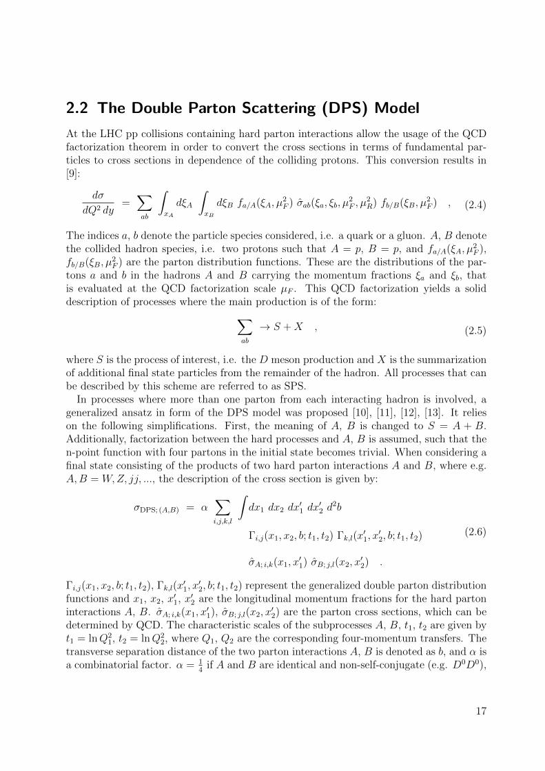
2.2 The Double Parton Scattering (DPS) Model
At the LHC pp collisions containing hard parton interactions allow the usage of the QCDfactorization theorem in order to convert the cross sections in terms of fundamental par-ticles to cross sections in dependence of the colliding protons. This conversion results in[9]:
dσ
dQ2 dy=∑ab
∫xA
dξA
∫xB
dξB fa/A(ξA, µ2F ) σab(ξa, ξb, µ
2F , µ
2R) fb/B(ξB, µ
2F ) , (2.4)
The indices a, b denote the particle species considered, i.e. a quark or a gluon. A, B denotethe collided hadron species, i.e. two protons such that A = p, B = p, and fa/A(ξA, µ
2F ),
fb/B(ξB, µ2F ) are the parton distribution functions. These are the distributions of the par-
tons a and b in the hadrons A and B carrying the momentum fractions ξa and ξb, thatis evaluated at the QCD factorization scale µF . This QCD factorization yields a soliddescription of processes where the main production is of the form:∑
ab
→ S +X , (2.5)
where S is the process of interest, i.e. the D meson production and X is the summarizationof additional final state particles from the remainder of the hadron. All processes that canbe described by this scheme are referred to as SPS.
In processes where more than one parton from each interacting hadron is involved, ageneralized ansatz in form of the DPS model was proposed [10], [11], [12], [13]. It relieson the following simplifications. First, the meaning of A, B is changed to S = A + B.Additionally, factorization between the hard processes and A, B is assumed, such that then-point function with four partons in the initial state becomes trivial. When considering afinal state consisting of the products of two hard parton interactions A and B, where e.g.A,B = W,Z, jj, ..., the description of the cross section is given by:
σDPS; (A,B) = α∑i,j,k,l
∫dx1 dx2 dx
′1 dx
′2 d
2b
Γi,j(x1, x2, b; t1, t2) Γk,l(x′1, x′2, b; t1, t2)
σA; i,k(x1, x′1) σB; j,l(x2, x
′2) .
(2.6)
Γi,j(x1, x2, b; t1, t2), Γk,l(x′1, x′2, b; t1, t2) represent the generalized double parton distribution
functions and x1, x2, x′1, x′2 are the longitudinal momentum fractions for the hard partoninteractions A, B. σA; i,k(x1, x
′1), σB; j,l(x2, x
′2) are the parton cross sections, which can be
determined by QCD. The characteristic scales of the subprocesses A, B, t1, t2 are given byt1 = lnQ2
1, t2 = lnQ22, where Q1, Q2 are the corresponding four-momentum transfers. The
transverse separation distance of the two parton interactions A, B is denoted as b, and α isa combinatorial factor. α = 1
4if A and B are identical and non-self-conjugate (e.g. D0D0),
17

α = 1 if A and B are different and either A or B is self-conjugate (e.g. JψD0) and α = 12
otherwise (e.g. D+D+) 1 .First, it is assumed, that Γi,j may be decomposed in terms of longitudinal and transverse
components:Γi,j(x1, x2, b; t1, t2) = Dij
h (x1, x2; t2, t2) F ij (b) . (2.7)
Further, the F ij (b) are assumed to be the same for all parton pairs ij involved in the
process of interest. Finally, it is assumed, that the longitudinal momentum correlationscan be ignored, such that the Dij
h factorize as:
Dijh (x1, x2; t2, t2) = Di
h(x1; t1) Djh(x2; t2) . (2.8)
Using these three simplifications, equation 2.6 can be rewritten as:
σDPS; (A,B) = ασSPS;A σSPS;B
σeff
, (2.9)
where SPS denotes the single parton scattering, and the effective cross section σeff is givenby:
σeff =
(∫d2b
(F ij (b)
)2)−1
. (2.10)
The approximations imply that the hard parton interactions are independent from eachother. They also violate energy conservation. Formula 4.2 is not justified, if the flavour ofthe partons or the momentum fractions make a difference in the studied processes. Nev-ertheless, this ansatz is phenomenologically successful and leads to an energy independentresult for the effective cross section σeff [14], [15] [16], [17]. Formula 4.2 does not rely ontheoretical predictions for the SPS cross section σSPS;A and σSPS;B, since there is no ex-plicit depencence on the parton distribution functions. Therefore, this model can be usedin regimes, where the uncertainty on the production cross section σ(A,B) is high, by usingmeasurements of σA and σB.
1The convention for α follows the addendum of [2] instead of the notation in [10].
18

3 Foundations: LHC Collider, LHCbDetector and Key Concepts for theAnalysis
The Large Hadron Collider Beauty Experiment (LHCb) is one of the four main experimentsat CERN, located at one of the four main collision points of the Large Hadron Collider(LHC) [19], [20]. The CERN, LHC accelerator and LHCb experiment are introduced inchapter 3.1, while chapter 3.1.1 explains the detector components of the LHCb experiment.In order to introduce the physical processes at the LHC accelerator and the LHCb expe-riment, the most important physical principles needed to understand the acceleration anddetection of particles are explained in chapter 3.1.2.
3.1 The LHC at CERN
CERN is the abbreviation for the European Organization for Nuclear Research, literallyConseil Europeen pour la Recherche Nucleaire. It was founded to plan the construction of aresearch laboratory for nuclear research [18]. The research started with the first acceleratorin 1957, a synchro-cyclotron. Shortly afterwards it was followed by the Proton Synchrotron(PS), which accelerated the first beams in November 1959 and is still operational today.Since then an increasing amount of large accelerators has been built. The most recent twoaccelerators in the history of CERN are the Large Electron Positron Collider (LEP) andthe Large Hadron Collider (LHC). The LEP accelerated electrons and positrons from 1989to 2000, while the LHC started to accelerate protons in 2009 and is still operating today.It was planned from the start during the first LHC studies in the 1980’s to reuse as muchof the LEP infrastructure as possible for the LHC, mainly the LEP tunnel. Along with theincreasing size and number of accelerators, the number of experiments and buildings grewmore and more. Today the CERN is one of the largest institutions worldwide with about10’000 visiting scientists representing over 600 universities and 100 nationalities.
The LHC accelerator is a proton proton collider with a circumference of 26.7 km. Itssize and experimental infrastructure turns the LHC into the currently largest and mostcomplicated scientific instrument in the world. The LHC is designed to be operated ata center of mass energy of
√s = 14 TeV and an instantaneous luminosity of LLHC =
2 · 1032 cm−2s−1. It consists of eight arcs with a length of 2.8 km and eight straightsections with a length of 500 m each. The tunnel housing the LHC lies between 45 m and170 m below the surface and has an inclination of 1.42% with respect to the horizontal
19

to enable an easier civil engineering. From 2010 to 2012 the LHC was operated at√s =
0.45, 2.76, 5.02, 7 and 8 TeV. To achieve such high center of mass energies, large bendingmagnets with a field strength of about 8 T are needed to keep the protons on track. Thisis achieved by superconducting magnets, which are cooled with superfluid helium at 1.9 K,implying the construction of a large cooling infrastructure with about 80 t of superfluidhelium.
The LHC is the last piece of a complicated chain of accelerators to produce, bunch andaccelerate the protons until they collide at one of the four collision points at the four mainexperiments. First, the protons are extracted as the nucleus of hydrogen atoms with an en-ergy of 50 keV. Then they are guided to a linear accelerator (LINAC), where their energyis increased to 50 MeV. Afterwards they are injected into a booster synchrotron which in-creases their energy to 1.4 GeV. Subsequently, the protons arrive at the proton synchrotron(PS) where they are not only accelerated but also grouped into a train of bunches. Thisstructure is kept until the proton beams finally collide in the LHC. The bunch-trains areinjected into the super proton synchrotron (SPS) and are again accelerated, this time tothe energy of 450 GeV. Then, they are transferred to the LHC ring via one of the transferlines. After the filling of both counter rotating beams with bunch-trains, the protons areaccelerated while the magnetic field in the bending dipoles is simultaneously rised untilthe collision energy is reached. Finally, the beams are brought to collision at the four col-lision points, where the four main detectors, Compact Muon Solenoid (CMS), A ToroidalLHC Apparatus (ATLAS), Large Hadron Collider Beauty Experiment (LHCb), A LargeIon Collider Experiment (ALICE) are situated. The beams can stay several hours in theLHC, if no technical problems occur, until they are finally dumped and the cycle is startedagain. This accelerator chain is shown in Fig. 3.1.
The locations, sizes and scopes of the four main experiments are different. ATLAS andCMS are general purpose detectors for high transverse momentum physics. LHCb is ab-physics experiment which focuses on CP-violation and rare decays of beauty and charmhadrons. It also performs analyses similar to ATLAS and CMS but in a different kinematicrange, for example W and Z production. ALICE investigates primordial states of matterlike the quark-gluon-plasma in heavy ion collisions.
20

CERNfaqLHCthe guide
LINAC 2
Gran Sasso
North Area
LINAC 3Ions
East Area
TI2TI8
TT41TT40
CTF3
TT2
TT10
TT60
e–
ALICE
ATLAS
LHCb
CMS
CNGS
neutrinos
neutrons
pp
SPS
ISOLDEBOOSTERAD
LEIR
n-ToF
LHC
PS
6794_07_LHC_cover_07_K2_wd.indd 1 14.01.2008 9:23:05 Uhr
Figure 3.1: Schematic overview of the accelerator chain for the LHC at CERN. This chainis started with the extraction of the protons from hydrogen atoms, followedby a linear accelerator (LINAC2), a booster synchrotron (BOOSTER), ProtonSynchrotron (PS), Super Proton Synchrotron (SPS) and the LHC (Figure takenfrom Ref. [21]).
21

3.1.1 The LHCb Detector
The LHCb detector is situated at one of the four main collision points of the LHC [22],[23]. It is a single-arm spectrometer with a forward geometry and is fully instrumented inthe pseudorapidity range of 2 < η < 5 (see Fig. 3.2, chapter 3.1.2).
The coordinate system for the LHCb is oriented, such that the positive z-axis pointsfrom the interaction point to the muon system along the beam pipe. The y-axis is vertical,starting from the interaction point to the surface, and is perpendicular to the LHC ring.The remaining x-axis, being perpendicular to the x- and y-axis, indicates where the bendingof the dipole magnet is most pronounced. Its forward design arises from the fact, that b andb quarks are produced in pairs and predominantly in the forward (or backward) direction.Therefore the LHCb forward geometry allows to detect a large fraction of the producedparticles containing a b or b quark, while covering a small solid angle, which helps reducingthe costs.
The LHCb’s subdetectors can be grouped into three parts. The track reconstructionsystem determines the three vector components of the particles’ momenta ~p. The purposeof the particle identification system is to determine the particle types. These two propertiescompletely describe each detected individual particle and describe therefore a good partof the full event. Finally, the trigger system selects the events of interest for the physicsanalyses.
• Track reconstructionThe track reconstruction system consists of a silicon microstrip detector called VertexLocator (VELO), placed closely to the interaction point. It measures precisely theposition of primary and secondary vertices as well as the impact parameter (IP)of the track. A second silicon microstrip detector, the Tracker Turicensis (TT), islocated before the dipole magnet. Hits in the TT are used to improve the momentumresolution of reconstructed tracks and reject pairs of tracks that in reality belongto the same particle. The tracking stations (T1, T2, T3), placed behind the dipolemagnet, use different technologies to detect particles: silicone microstrips close to thebeam pipe and straw-tubes in the outer regions. The dipole magnet itself completesthe track reconstruction system. Its magnetic field with vertical field lines bendsthe flight path of the particles in the xz - plane. Therefore the size of the magneticfield allows the determination of the patricles’ momenta by comparision of the trackdirection before and after the magnet. All tracking detectors are characterized by ahigh spatial resolution (in one or two spatial coordinates) and a low material budget.
• Particle identificatonThe particle identification system uses different physical principles. The two RingImaging Cherenkov Detectors (RICH1, RICH2) use the Cherenkov Effect to dis-tinguish between different types of hadrons. The consecutive electromagnetic andhadronic calorimeters (ECAL, HCAL) measure the energy of the impinging particlesby fully absorbing them. The ECAL absorbs all electromagnetic showers but only asmall part of the hadronic showers, while hadronic showers are contained in the big-
22

ger HCAL. Two smaller subdetectors, the scintillating pad detector (SPD) and thepreshower detector (PS), in front of the ECAL supplement the calorimeter systemby resolving ambiguities on the identification. For instance, the SPD allows the dis-crimination of electron and photon candidates, while the PS is used to discriminateelectron and photon candidates from hadron candidates. The muon system consistsof five stations (M1 to M5) and is placed at the most remote position within theLHCb seen from the interaction point. It identifies muons, that traverse the detectorand the iron shields between the muon stations almost unaffected.
• TriggerThe LHCb detector produces too much information per collision for all of it to beread out. Moreover, many of the collisions are not of particular interest for physicsanalyses. Therefore the LHCb has a three stage trigger system to reduce the amountof data collected to a rate, which can be written to disk. The first level, called L0,is hardware based, while the second and third stage, HLT1 and HLT2, are softwarebased and execute algorithms that partially reconstruct the event and then decide ifthey are of further interest or not.
23

M1
M3
M2
M4
M5
RICH2
HCAL
ECAL
SPD/PS
Sid
e View
Magnet
z5m
y
5m
10m
15m
20m
TT
RICH1
T1T2T3
Vertex
Locator
Figu
re3.2:
Sch
ematic
side
view
ofth
eL
HC
bdetector.
The
diff
erent
sub
detectors
arefrom
the
leftto
the
right
inth
eforw
ardb
eamdirection
:T
he
vertexlo
cator(V
EL
O),
the
two
Rin
gIm
aging
Cheren
kovD
etectors(R
ICH
1an
dR
ICH
2),th
etrack
ing
stations
(TT
and
T1-T
3),th
escin
tillatorpad
detector
(SP
D),
the
presh
ower
(PS),
the
electromagn
eticcalorim
eter(E
CA
L),
the
had
ronic
calorimeter
(HC
AL
)an
dth
em
uon
stations
(M1-M
5).F
igure
takenfrom
Ref.[22],
[23].
24

3.1.2 Key Concepts for the Analysis
This analysis requires the understanding of some fundamental principles of experimentalparticle physics. The most important ones are explained in this section.
There are two major variables describing the dataset at hands: the center of mass energys, also denoted as
√s, and the luminosity L.
Center-of-Mass Energy√s√s√s
At the LHC, predominantly two protons are collided with each other. The LHC is in factable to collide also heavy ions with each other or protons with heavy ions, but since suchdata is not used in this analysis, pp collision is assumed in the following. The two protonshave the same rest mass m1 = m2 and the four-momenta pµ1 = (E1/c , ~p1), pµ2 = (E2/c , ~p2)where the energy E1 = E2 and momenta ~p1 = −~p2 are given in the center of mass frameand c = 2.998 ·108 m/s is the speed of light. The Mandelstam variable s, also called centerof mass energy, is defined by:
s = (pµ1 + pµ2)2 = (E1/c+ E2/c)2 . (3.1)
Since (pµ1 + pµ2)2 = M2c4, s is the square of the invariant mass M . Natural units, where~ = c = 1, are used throughout this analysis. For clarity an explicit factor c is preservedin selected equations. The center of mass energy can also be denoted as square root andin natural units: √
s = (pµ1 + pµ2) = (E1 + E2) = M . (3.2)
The data used in this analysis were taken at a center of mass energy√s = 2.76 TeV.
Luminosity LLLThe luminosity is a measure of how many collisions happen when two bunches of particlescollide with each other and is linked to the number of collisions and the cross section by:
dN
dt= L σ ,
wheredN
dt: number of collisions per second
σ : cross section
L : (instantaneous) luminosity
(3.3)
25
For a gaussian beam distribution, the luminosity L is given by:
L =N2b nb frev γ
4π εn β∗F ,
where Nb : number of particles per bunch
nb : number of bunches per beam
frev : revolution frequency
γ : relativistic gamma factor
εn : normalized transverse beam emittance
β∗ : Beta function at the collision point
F : geometrical luminosity reduction factor .
(3.4)
The beta function at the collision point β∗ is a measure of how compressed the beamis at the collision point. The normalized transverse beam emittance εn is a measure ofthe distribution of the particles in space and momentum. The geometrical luminosityreduction factor F takes into account, that the beams do not collide head on and arisesdue to the crossing angle at the collision point. The luminosity L has the units of inversearea and inverse time, given in by the SI units m−2 s−1 or more practical by b−1 s−1, wherethe unit barn is given by the relation 1 b = 10−28m2. The integrated luminosity givenby L =
∫Ldt is a measure for the total amount of the aquired data. The used dataset
corresponds to an integrated luminosity of L = 3.31 pb−1.
Invariant Mass MMMSince the velocity ~v is frequently close to c in particle physics, relativistic conservation lawsfor energy and momentum have to be used. The energy E and momentum ~p from classicalmechanics are reformulated as the four-momentum pµ, in order to adapt to Einstein’sprinciples of relativity, implying Lorentz transformations and the introduction of the four-vector notation, when considering space-time translations (see [24], [25]). Consequently,the two conservation laws from classical mechanics are reformulated into one, called the(relativistic) energy-momentum conservation or four-momentum conservation:
26

∑i
pµ = const. ,
where pµ =(p0, ~p
)= γ M (c, ~v ) four-momentum
xµ = (c t, ~x ) (contravariant) four-position vector
x0 = ct time component or zero component
~x : space component
dτ =dt
γproper time element
γ =1√
1− β2
β =~v 2
c2
M : invariant mass, also called rest mass in the particle’s
rest frame of reference
E = p0 c = γ M c2 total energy
E|~v=0 = E0 = M c2 rest energy
T = E − E0 = M c2 (γ − 1) kinetic energy .
(3.5)
This holds under the condition of the Lorentz invariance of the four-momentum squared,p2, resulting in the energy momentum relation:
p2 = 〈pµ, pν〉 =(p0)2 − ~p 2 =
E2
c2− ~p 2
= γ2M2c2 − γ2M2~v 2 = M2γ2(c2 − ~v 2
)= M2 1
1− ~v 2
c2
(c2 − ~v 2
)= M2c2 ,
where 〈xµ, yν〉 =3∑
µ=0
3∑ν=0
gµνxµyν = gµνx
µyν = xµyµ = x0y0 − ~x · ~y
gµν = gµν =
1 0 0 00 −1 0 00 0 −1 00 0 0 −1
Metric Tensor .
Simpler: E2 = M2c4 + ~p 2c2
(3.6)
27

Therefore the invariant mass M is the same in all inertial frames of reference. In the restframe of the particle, the invariant mass M is equal to the energy E of the particle (dividedby c2) and is called rest mass.
Consider a particle, which decays into N daughter particles. Since the four-momentumpµ is conserved, the invariant mass of the decay particle, M , can be calculated as a sum ofthe energies and momenta of the daughter particles using the energy-momentum relation:
(Mc2
)2=
(N∑i
Ei
)2
−
(N∑i
~pi c
)2
,
where M : Invariant mass of the system of particles,
equal to the invariant mass of the decay particle
Ei : Energy of the daughter particle i
~pi : Momentum of the daughter particle i
c = 2.998 · 108 m/s Speed of light; when natural units are used: ~ = c = 1(3.7)
For one particle that decays into two daughter particles this relation becomes:
M2c4 = (E1 + E2)2 − (~p1 + ~p2)2 = m21 c
4 +m22 c
4 + 2(E1E2 − ~p1 ~p2 c
2)
= (pµ1 + pµ2)2 ,
where m1,2 : invariant masses of the daughter particles
E1,2 : energies of the daughter particles
pµ1,2 : four momenta of the daughter particles .(3.8)
This concept is applied in this work by starting from experimentally reconstructed trackswhich correspond to a measurement of ~p. Using other subdetectors, those tracks get a Pionor Kaon hypothesis assigned. This leads to particle candidates with p0 = E determined byp2 = m2
K or p2 = m2π. D meson candidates are formed by adding the momenta of the decay
products, e.g. for D0, D+: pµD0 = pµK− + pµπ+ , pµD+ = pµK− + pµπ+ + pµπ+ . The comparisonto the known D mass provides a discriminant with respect to other processes.
28

Transverse Momentum pT , Longitudinal Momentum pLAs two protons collide at the LHCb interaction point, they form a PV, of which a bunch ofparticles with momentum ~pi , i ∈ {1, ..., n} emerge. Each momentum ~pi can be decomposedinto the transverse momentum ~pi
T perpendicular to the beam axis and the longitudinalmomentum ~piL along the beam axis. The same principle holds for the energies Ei , i ∈{1, ..., n}, and consequently for the four momenta pµ , i ∈ {1, ..., n}. Moreover such adecomposition can be applied at each vertex.
z
y
x
beam line
LHCb forward region
pp
PV
~pi
θcm
~piT
~piL
Figure 3.3: Schematic illustration of the decomposition of the momentum of a particle ~piemerging from a PV into longitudinal- and transverse momentum ~piL and ~pi
T .
Pseudorapidity ηηη and Rapidity yyyThe longitudinal pseudorapidity η of a particle is defined as:
η := − ln
(tan
(θcm
2
))=
1
2ln
(|~p|+ |~pL||~p| − |~pL|
)= arctan
(|~pL||~p|
). (3.9)
The longitudinal momentum pL is the momentum component along the beam axis, givenalong the positive z-axis in the forward coordinate system of LHCb. θcm is the scatteringangle between the momentum of the particle in question, ~p, and the beam axis (z-axis).The pseudorapidity is a commonly used variable at hadron colliders. It is defined as thehigh relativistic limit of the longitudinal rapidity y, given by:
y := arctan
(~v
c
)= arctan
(|~pL| cE
)=
1
2ln
(E + |~pL|cE − |~pL|c
). (3.10)
In the relativistic limit ~p ≈ E or M << pT , the pseudorapidity η is a good approxima-tion of the longitudinal rapidity y, i.e. η ≈ y. Experimentally, these quantities have thefollowing advantages compared to the angle. Differences in rapidity or pseudorapidity are
29

Lorentz invariant under boosts along the beam axis, i.e. they transform additively, similarto velocities under Galilean transformations. Loosely spoken, the particle production isconstant as a function of rapidity (and pseudorapidity, if the mass of the particle is negli-gible compared to its energy). The pseudorapitiy is a pure geometrical quantity and onlyrelated to the scattering angle θcm. When the interaction point is fixed, each detector ele-ment can get a pseudorapidity value assigned. Consequently, the LHCb detector elementsare positioned at high η, which allows the measurements of particles produced at highrapidity y.
Impact Parameter IPIPIPIt is defined as the shortest distance of a track to the PV. It is schematically illustratedin Fig. 3.4 for the example of a D0 candidate promptly produced in the PV with decaymode D0 → K− π+, resulting in a Kaon and a Pion track. The reconstruction of the D0
candidate yields usually also a non-zero but very small IP for the D0. Candidates producedin PV’s can be distinguished from the ones produced in SV’s by applying a specific cut onthe impact parameter for the candidate.
z
y
x
beam line
PVLHCb forward region
D0
SV
π+
K−
IPπ+
IPK−
Figure 3.4: Schematical illustration of the impact parameter (IP) using the example of aD0 candidate promptly produced in a PV with decay mode D0 → K− π+.
30

Branching Fraction or Branching Ratio BiBiBi
The Branching fraction for a certain decay is the fraction of particles, which decay by anindividual decay mode i, Ni, with respect to the total number of particles decaying, Ntot,given by:
Bi =Ni
Ntot
. (3.11)
For instance, the charmed meson D0 has a branching fraction of BD0→K− π+ = 3.93% forthe decay mode D0 → K−π+ and BD0→K+ π− = 1.49 · 10−4 for D0 → K+π−.
Hypothesis TestingIn chapter 4.4, three goodness of fit criteria are imposed in order to estimate the fit qualityof unbinned maximum likelihood fits to tracks, vertices, envent hypotheses and invariantmass distributions. Moreover, χ2/ndof values are used by the different reconstruction soft-wares to estimate the goodness of fits in chapter 4.2.1. These criteria are explained in thefollowing (see also [26], [27]).
1) Reduced χ2, i.e. χ2/ndof:Assume an unbinned one-dimensional distribution of an observable x that has beenfitted by an unbinned maximum likelihood fit with a model f(x). Furthermore as-sume a subsequently applied binning to the distribution. The reduced χ2 value isgiven by:
χ2/ndof =1
ndof
∑i
(y(xi)− f(xi))2
σ2y(xi)
,
where y(xi) : y-value of a data point or bin at position xi
f(xi) : fit function value at the position xi
σy(xi) : error on y(xi) .
(3.12)
The number of degrees of freedom is given by ndof = nb−np, where nb is the number ofbins or data points and np is the number of fit parameters that had to be determined.
2) Upper tail probability or upper P-value of the χ2 distribution, Pu(χ2, ndof):
This quantity is given by:
Pu(χ2, ndof) =
1
2ndof
2 Γ(ndof
2
) ∫ ∞χ2
tndof
2− 1 e−
t2 dt
where χ2 : χ2 value (see equation 3.12) ,
ndof : number of degrees of freedom
Γ(z) =
∫ ∞0
tz−1 e−t dt Gamma function (Euler’s integral form) .
(3.13)
31
It denotes the probability to observe a χ2-value, that is greater than the given χ2-value, provided the underlying hypothesis is true. Its analogon is the lower tailprobability or lower P-value, Pl(χ
2, ndof), representing the probability to observe aχ2 value, that is smaller than the given one. It is given by:
Pl(χ2, ndof) =
1
2ndof
2 Γ(ndof
2
) ∫ χ2
0
tndof
2− 1 e−
t2 dt . (3.14)
Pu(χ2, ndof), Pl(χ
2, ndof) are connected to the χ2 distribution, whose probability den-sity function (PDF) is given by:
χ2(x;ndof) =1
2ndof
2 Γ(ndof
2
) xndof2− 1 e−
x2 . (3.15)
The cumulative distribution function (CDF) of the χ2 distribution, C(χ2(x;ndof)),can be splitted into Pu(χ
2, ndof), Pl(χ2, ndof) by:
C(χ2(x;ndof)) =1
2ndof
2 Γ(ndof
2
) ∫ ∞0
tndof
2− 1 e−
t2 dt
=1
2ndof
2 Γ(ndof
2
) (∫ χ2
0
tndof
2− 1 e−
t2 dt +
∫ ∞χ2
tndof
2− 1 e−
t2 dt
)= Pl(χ
2, ndof) + Pu(χ2, ndof) .
(3.16)The χ2 PDF is a special case of the Gamma PDF, given by:
G(x; b, p) =bp
Γ(p)xp−1 e−bx , (3.17)
when its free parameters b > 0 and p > 0 are defined as b = 1/2, p = ndof/2. Sincethe Gamma CDF, C(G(x; b, p)), can be expressed as a form of the lower regularizedincomplete Gamma function γl(x; k) by:
C(G(x; b, p)) =γl(b x, p)
Γ(p)=
1
Γ(p)
∫ b x
0
tp−1e−t dt , (3.18)
all so far mentioned CDF’s are forms of the lower- or upper regularized incompleteGamma functions γl(x, k), γu(x, k), especially Pl(χ
2, ndof), Pu(χ2, ndof).
3) Pull values pi:Assume an unbinned one-dimensional distribution of an observable x, that has beenfitted by an unbinned maximum likelihood fit with a model f(x). Moreover assumea subsequently applied binning to the distribution. The pull value pi of a certain bin
32

i is defined by:
pi =y(xi)− f(xi)
σy(xi)
,
where y(xi) : y-value of a data point or bin at position xi
f(xi) : fit function value at the position xi
σy(xi) : error on y(xi) .
(3.19)
The calculated pull values for all bins, pi, result in a pull distribution.
33

4 Cross Section Determination
The so far measured double open charm production cross sections in pp collisions at LHCbat√s = 7 TeV (see [2], [3]) are supplemented by such a measurement at
√s = 2.76 TeV.
The LHCb experiment collected data from pp collisions at a center of mass energy of√s = 2.76 TeV and with an integrated luminosity of L = 3.3 pb−1 during the time
period starting from Feb. 12, 2013 until Feb. 14, 2013. After this period, the LHC and allassociated experiments were shut down for maintenance and upgrades.
One group of particle candidates, which can originate from pp interactions are the ones,that contain at least a charm quark, the charm hadrons C. One subgroup thereof is thegroup of the charm mesons, the other is the group of the charm baryons. Typical elementsin the group of charm mesons are the D0 = cu, D = cu, D+ = cd, D− = cd particles.Such charm mesons can also occur twice as CC. When this doublet contains two charmquarks or two anti-charm quarks, it is referred to as double open charm production, whenit comprises a charm and an anti-charm quark, it is referred to as charm pair production.For this analysis the notation of a charm state C includes its anti-particle state C. Thisimplication of the full charge conjugation results in the fact, that e.g. D0D0 denotes{D0D0, D0D0}, and D0D0 denotes {D0D0, D0D0}.
The main objective of this analysis is to measure the production cross sections for thesingle open charm mesons C, double open charm mesons CC and charm pair producedmesons CC, where C ∈ {D0, D+}, C ∈ {D0, D−}. The determination of the productioncross section at LHCb involves a chain of analyses. Chapter 4.1 provides the strategy of themeasurement. The charm event candidates need to be identified and isolated from otherparticle candidates in the data. This is achieved by a system of selection criteria, explainedin chapter 4.2. Moreover, it covers the pile-up and feed-down, being two typical backgroundprocesses, especially when double open charm event candidates are involved. Chapter 4.3gives an overview of the charm candidates passing the selections. The remaining chapters,i.e. chapter 4.4, 4.5, 4.6, 4.7, 4.8, deal with the different terms of the production crosssection formula listed in chapter 4.1 (see equation 4.1). The final chapter 4.9 covers thecalculation of the systematic uncertainties in the determination of the production crosssection.
34

4.1 Analysis Strategy
The analysis strategy outlines the procedures, which need to be executed on the datacollected by LHCb, in order to get a production cross section for the single open charmmeson candidates D0 and D+ and double open charm event candidates D0D0, D0D+ andD+D+. For comparison, the production cross sections for the charm pair production eventcandidates D0D0, D0D− and D+D− are also determined. This analysis strategy is basedon the one described in [2], [3].
As a first step the LHCb detector collects electric signals, which are created by theinteraction of particles with the matter of the detector components, and which form theunfiltered data. This data is passed through the data acquisition sytem (DAQ) of theLHCb detector, whose capabilities are mainly limited by the trigger, and is filtered, suchthat it can be stored permanently on hard disks. This filtering involves the trigger selection,in order to reduce the nominal interaction rate from about 20 − 30 MHz to 1 − 15 kHz.This process needs to be executed online, i.e. while the data was taken. Afterwards,the triggered data is stored on disk. All following processing steps are therefore executedoffline, i.e. when the data taking was finished.
In a second step, the stored data is reconstructed using Reco14 and subsequently filteredby the Stripping21 algorithm. In this process, the charm event candidates C and CC, whereC ∈ {D0, D+} are created from their decay products, the K− and π+ track candidates. Allthese candidates are further selected, which is achieved by the stripping selection describedin chapter 4.2.1. Due to the short lifetime of the open charm event candidates, they need tobe reconstructed from their decay products. For this analysis the decay modes D0 → K−π+
and D+ → K−π+π+ are chosen, because they fulfill several requirements [7]. First, thedecay modes result in a low number of daughter particles, such that the initial momentumsplits into few decay products. Secondly, the branching ratio Bi of the decay modes needto be high enough, such that the corresponding reconstructed mesons are sufficient innumbers for a measurement. This is explained in more detail in chapter 4.3 and 4.4.Thirdly, the event candidates are supposed to be detected as precise as possible by theLHCb detector. This means, that all decay products can be detected directly and shouldbe charged. Fourthly, the decay modes are flavour tagging, such that the charm candidatecan be distinguished from its anti particle. This enables the differentiation between doubleopen charm production and open charm pair production.
The third and final step of filtering is the offline selection. It consists of the selectionneeded to be applied, in order to match the definition of the efficiencies (see chapter4.6). Most of the efficiencies, being acceptance εacc, reconstruction and selection efficiencyεrec and particle identification (PID) efficiency εPID, are not calculated explicitely for thisanalysis, but taken from the analysis of associated production of Υ and open charm [28],[29]. In order for the efficiencies to be applicable, the same selection as for the efficiencycalculation done in the analysis [28], [29] needs to be applied for this analysis as describedin chapter 4.2.1. An important difference to the previous works is, that [28], [29] did nottrigger on the open charm, but on µ±. After the selection process, the different backgroundcontributions of pile-up and feed-down are investigated in chapter 4.2.2.
35

The production cross sections for the single open charm event candidates D0, D+ andthe double open charm event candidates D0D0, D0D+, D+D+ in pp collisions at LHCbcan be calculated as:
Single Charm: σC =Nc; s;C
L BC εGEC;C
Double Charm: σCC =Nc; s;CC
L BC BC εGEC;CC
,
where Nc; s : efficiency corrected signal yield
L : integrated luminosity
B : branching ratio
εGEC : global event cut efficiency
C ∈ {D0, D+} : single open charm event candidate(s)
CC , C ∈ {D0, D+} : double open charm event candidates .
(4.1)
The simple factorized ansatz of the DPS model (see chapter 2.2) predicts, that the effectivecross section, σeff is constant and independent of the process and the center of mass energy√s. Assuming no contamination from soft processes, it is given by:
σCC = ασC σCσeff
,
where σC , C ∈ {D0, D+} : cross sections for the single open charm
event candidates
σCC : cross-section for the double open charm event candidates
α =
{1/4 , D0D0 , D+D+
1/2 , D0D+combinatorial factor .
(4.2)
The measurements of J/ψC together with the predictions in [2], [3] suggest, that thecontamination from the hard process gg → cccc is indeed small. Formula 4.2 is sometimesreferred to as Pocket Formula. It can be solved for σeff leading to:
σeff = ασC σCσCC
. (4.3)
Being a ratio of cross sections, this equation has the advantage, that several systematicuncertainties both in experimental determination as well as in theory calculations do cancelout. The calculation of the terms, which arise in equation 4.1, are explained in chapters4.4, 4.5, 4.6, 4.7, 4.8.
36

4.2 Event Selection and Background Determination
In the following, the event selection is described, which includes the trigger selection,stripping selection for the Stripping21 algorithm and the offline selection. These selectionprocesses are the first step in eliminating the background, and are explained in chapter4.2.1. The influence of two specific types of background, called pileup and feed-down, onthe signal of the charm event candidates is described in chapter 4.2.2. The second back-ground elimination step is achieved by the calculation of the efficiency corrected yields Nc; s
in chapter 4.5.
4.2.1 Event Selection
The data from pp collisions collected by the LHCb detector with a center of mass energyof√s = 2.76 TeV has the production identification number 23836 and the run number
interval [137147, 137312] 1. This unfiltered data passes three selection steps.The first step of selection is the trigger selection, which is done online. The data was
taken with the trigger configuration key (TCK) 0x00A90046, a TCK that was used pre-viously in the high integrated luminosity data taking at
√s = 8 TeV in 2012. The trig-
ger has three stages, the hardware stage L0 and the two software stages Hlt1 and Hlt2.The trigger selection relies on HCAL clusters in L0, a non prompt high pT track in Hlt1and the D0 → K−π+, D+ → K−π+π+ candidates in Hlt2. The names of the triggerlines are L0Hadron for L0, Hlt1TrackAllL0 for Hlt1, Hlt2CharmHadD02KPi for D0 resp.Hlt2CharmHadD2HHH for D+ for Hlt2 and are listed in Tab. 4.1. One cut appliedat the trigger level is APT > 2 GeV for the charm, which translates approximately topT > 2 GeV. Due to the calculation of the trigger efficiency (see chapter 4.6), every singleopen charm event candidate is required to be triggered on signal (TOS). In the case ofdouble open charm or open charm pair production event candidates, at least one of thetwo single open charm event candidates is required to be TOS. Previous analyses, like[28], [29], benefit from using µ± for the trigger. Compared to hadrons, like K± and π±,muons are relatively easy to identify by the LHCb muon system and are much less freqent.Therefore the trigger has a lot more work to do when using the L0Hadron trigger instead ofthe L0Muon trigger. Consequently, the L0Hadron trigger involves harder global event cuts(GEC), in order to keep the readout rate of the trigger within the maximum permissiblelimit. Moreover, the trigger was not optimized for a low center of mass energy and lowinstantaneous resp. integrated luminosity, which can be an issue for this analysis. Thisissue and the resulting consequences are specified further in chapter 4.6, 4.9 and 5.
1This data can be found in the LHCb Dirac Bookkeeping system underLHCb/Collision13/Beam1380GeV-VeloClosed-MagDown/Real Data/Reco14/90000000 ( Full stream )/FULL.DSTor in the LHCb run database by a search for the run number.
37

Candidate Trigger stage Trigger line
D0, D+ L0 L0Hadron
D0, D+ Hlt1 Hlt1TrackAllL0
D0 Hlt2 Hlt2CharmHadD02KPi
D+ Hlt2CharmHadD2HHH
Table 4.1: Trigger lines used for the selection of events matching the decay modes D0 →K−π+, D+ → K−π+π+.
The two remaining selection steps, stripping- and offline selection, are done offline. Thestripping selection consists of the Stripping21 algorithm implemented in the strippingLHCb software framework. The used stripping lines are StrippingD02KpiForPromptCharm,StrippingDForPromptCharm, StrippingDiCharmForPromptCharm. Stripping21 selects thetriggered data according to the chosen decay modes and the stripping selection criteria,which help to reduce the background. The selection criteria of the stripping- and offlineselection are combined into one set, which is splitted into three categories. The first ca-tegory contains the selection criteria applied on the decay candidates of the decay modesD0 → K−π+, D+ → K−π+π+, the K− and π+ meson candidates. The criteria can bestructured in criteria for track reconstruction and PID:
• A good track reconstruction quality is ensured by requiring four criteria for eachtrack event candidate.
First, the χ2trk/ndof provided by the track fit is χ2
trk/ndof < 3. The track reconstructionsoftware checks for hit patterns, which can form a potential K− or π+ track, andcombines these hit patterns to track candidates using a fit, called track fit. Since theamount of measurement points is limited and the charged track candidates can scatterin the detector material, wrong combinations of hit patterns can be reconstructed as atrack. In order to quantify the goodness of the track fit, the distances between the hitpoints and the track are summed up and divided by their experimental uncertaintyand the number of degrees of freedom ndof, yielding χ2
trk/ndof = 1ndof
∑ y(xi)−f(xi)σy(xi)
(see
also chapter 3.1.2).
Secondly, the transverse momentum is pT > 0.25 GeV.
Thirdly, the track ghost probability has to be Ptr < 0.5. Ghost tracks are tracks,which are reconstructed from random hit points by mistake.
Fourthly, to suppress any contribution from duplicate tracks created by the recon-struction, only candidates with a symmetric Kullback-Leibler divergence, ∆KL, cal-culated with respect to all candidates in the event, of ∆KL > 5000 are considered[30], [31], [32].
In addition, K−, π+ used for the reconstruction of long lived charm particles, arerequired not to be produced in primary interaction vertices (PV). To ensure this, only
38
candidates with a χ2 of the impact parameter, χ2IP, with respect to all reconstrcted
PV’s, of χ2IP > 9 are considered. At LHCb, the χ2
IP is calculated as the increase ofthe χ2
vx of the PV, if one additional track is added to the vertex fit. This can be
approximated by χ2IP '
(IPσIP
)2
.
• A PID of good quality is ensured by requiring the following criteria for each trackevent candidate.
The track must have left a signal in the RICH detectors catched by its PID system,fulfilled by HASRICH = True [42].
The momentum, p, required to be in the range 3.2 GeV < p < 100 GeV and thepseudorapidity, η, within 2 < η < 4.9 ensure a good acceptance in the RICH.
To select well identified K− (π+), the combined probabilty of the K− (π+), PK−
(Pπ+) is required to be Pl < 0.1 , l ∈ {K−, π+}. This quantity is the output of anartificial neural net using mainly the Log-Likelihood, logL, of the K−, π+ hypothesisfrom the RICH reconstruction [42].
In addition, the difference in the Log-Likelihood of the K− hypothesis with respectto the π+ hypothesis, ∆K−/π+ logL, is required to be ∆K−/π+ logL > −5. In orderto quantify the hypothesis, the RICH and the calorimeters are used [42].
These selection criteria are summarized in Tab. 4.2.
39

Candiate(s) Variable Cut LOKI functor
Track Reconstruction
K−, π+ χ2tr/ndof < 3 TRCHI2DOF
pT [GeV] > 0.25 PT
Ptr, gh < 0.5 TRGHOSTPROB
∆KL > 5000 CLONEDIST
χ2IP > 9 MIPCHI2DV
Particle Identification
K−, π+ HASRICH True HASRICH
p [GeV] 3.2 < p < 100 P
η 2 < η < 4.9 ETA
K− PK− > 0.1 PROBNNK
∆K−/π+ logL > −5 PIDK
π+ Pπ > 0.1 PROBNNpi
Table 4.2: Selection criteria for theK− and π+ track candidates, used for the reconstructionof the single open charmed event candidates D0 and D+.
The selected K− and π+ are then combined to form the single open charm event candi-dates D0, D+ with corresponding decay modes D0 → K−π+, D+ → K−π+π+. The secondcategory of selection criteria contains the criteria applied on these open charm event can-didates. The criteria can be structured in criteria for the decay chain, the primary vertex(PV) and the pile-up resp. feed-down:
• The K−, π+ track candidates shall originate from the open charm event candidates.This is achieved by a vertex fit performed by the vertex reconstruction software, whichcombines the K− and π+ tracks to vertices. The goodness of this fit is estimatedby the χ2
vx, which is required to be χ2vx < 9 for the D0 and χ2
vx < 25 for the D+
candidates.
In addition, the transverse momentum of the open charm event candidates has to bewithin 2 < pT < 20 GeV, and the rapidity in the range 2 < y < 4.5.
• To ensure that the charm meson candidates originate from a PV, the χ2IP of these
candidates with respect to any of the reconstructed PV’s is required to be χ2IP < 9.
Moreover, the decay time c τ of the candidates is required to be c τ > 100 µm. Thisquantity is extracted from a lifetime fit, which calculates the distance between the
40

best PV and the decay vertex of the candidates. The PV is determined by the vertexfit as the vertex, which has the smallest distance to the interaction point. The bestPV is the PV, which has the smallest χ2
vx, calculated by the vertex fit.
• In order to remove background from pile-up and feed-down (see chapter 4.2.2), it isrequired, that the momentum direction is consistent with the flight direction calcu-lated from the PV’s and SV’s. This is acquired by a decay tree fit performed bythe DecayTreeFitter tool, which combines vertices to decay chains for the candidates[33]. The χ2
dtf/ndof of this fit gives an estimate of its goodness and is required to beχ2
dtf/ndof < 5.
The invariant mass window for the open charm event candidates of 1.820 < MC <1.920 GeV, where C ∈ {D0, D+}, is applied.
The selection criteria for the single open charm event candidates are summarized inTab. 4.3.
Candidate Variable Cut LOKI functor
D0 χ2vx < 9 VFASPF(VCHI2)
pT [GeV] 2 < pT < 20 PT
y 2 < y < 4.5 RAP
χ2IP < 9 MIPCHI2DV
cτ [µm] > 100 BPVLTIME(9) · c light
χ2dtf/ndof < 5 DTF CHI2NDOF
M [GeV] 1.820 < M < 1.920 M
D+ χ2vx < 25 VFASPF(VCHI2)
pT [GeV] 1 < pT < 20 PT
y 2 < y < 4.5 RAP
χ2IP < 9 MIPCHI2DV
cτ [µm] > 100 BPVLTIME(9) · c light
χ2dtf/ndof < 5 DTF CHI2NDOF
M [GeV] 1.820 < M < 1.920 M
Table 4.3: Selection criteria used for the selection of the single open charm event candidatesD0, D+.
Subsequently, the selected single open charm event candidates D0, D+ are paired toform the double open charm event candidates D0D0, D0D+ and D+D+. In addition, thecharm pair production candidates D0D0, D0D−, D+D− are studied. The third category
41

of selection criteria contains the sole criterium applied on these double open charm andcharm pair production event candidates:
• In order to reject background from pile-up and feed-down, it is required, that themomentum direction is consistent with the flight direction calculated from the lo-cations of the PV’s and SV’s. This is aquired analogously by the DecayTreeFittertool as for the single open charm event candidates. The corresponding χ2
dtf/ndof isrequired to be χ2
dtf/ndof < 5.
This selection criteria is listed in Tab. 4.4.
Candiate(s) Variable Cut LOKI functor
D0D0, D0D+, D+D+, χ2dtf/ndof < 5 DTF CHI2NDOF
D0D0, D0D−, D+D−
Table 4.4: Selection criterion used for the selection of the double open charm event candi-dates and charm pair production event candidates.
4.2.2 Pile-Up and Feed-Down
Sometimes it can happen, that two pp collisions occur too close for the detector to distin-guish. This canal produces two D mesons falsely identified as double open charm and isreferred to as pile-up. The background contributions from pile-up and feed-down in thedata are treated using a method that exploits the cut on χ2
dtf/ndof [2], [3]. Events for whichthe two charm mesons come from the same PV, the following decomposition can be used:
χ2dtf/ndof CC = χ2
dtf/ndof C + χ2dtf/ndof C ,
where χ2dtf/ndof : χ2 per number of degrees of freedom
of the fit using the DecayTreeFitter tool [33]
C ∈ {D0, D+} : single open charm event candidates .
(4.4)
This identity is exact, if the position of the PV does not change, when the final state tracks(the K−, π+) of the charm meson candidates are successively removed, when the PV isrefitted. Since the PV position does change a little, the identity is valid up to relativelysmall corrections. For pileup events, an additional contribution, the χ2/ndof of the decay-tree-fitter distance between the two PV’s of the charm mesons, χ2
dtf/ndof PV-dist, adds toequation 4.4. This contribution is in general substantial, as for instance demonstrated for
42

the distance in the z-direction δz and its uncertainty σδz:
χ2dtf/ndof PV-dist =
(δz
σδz
)2
+ ... >
(δz
σδz
)2
≈(
5 cm
0.2 mm
)2
= 6.25 · 104
where δz : Distance in z-direction of the two PV’s
for the charm meson candidates in the case of pileup
σδz : Uncertainty on the distance δz
(4.5)
Therefore, all events with log10(χ2dtf/ndof CC) > 5 can be treated as pileup up to the
mentioned small corrections.The contribution from pileup into the signal region χ2
dtf/ndof CC < 5, equal tolog10(χ2
dtf/ndof CC) . 0.7, can be estimated by studying the shape of the χ2dtf/ndof CC
distribution separately in the pileup region log10(χ2dtf/ndof CC) > 5. From a fit to the
χ2dtf/ndof CC distribution in the pileup region, the contribution from pileup can be extracted
and subsequently extrapolated into the signal region. This process is illustrated inFig. 4.1 a), which shows the χ2
dtf/ndof distribution for D0 + Track candidates, fitted by amodel consisting of four Gamma distributions, one each for the signal, the pile-up and thetwo feed-down peaks [34], [35].
The χ2dtf/ndof CC distributions for this analysis are shown in Fig. 4.1 b), c), d). All
χ2dtf/ndof CC distributions contain no events in the pileup region log10(χ2
dtf/ndof CC) > 5.Therefore it is concluded, that the pile-up contribution is negligible. Very low or no pile-upis expected, since the data are taken at low pile-up conditions with an average number ofvisible interactions of about one (µ ' 1).
Another contribution of background, called feed-down, needs to be considered. The termfeed-down is used, since charm mesons can originate from the decay of B mesons. Such afeed-down contribution is present in the χ2
dtf/ndof CC distribution at lower values than thecontribution from pile-up, i.e. approximately in the region log10(χ2
dtf/ndof CC) ∈ [1, 4.5].D mesons originating from B decays do have a small but significant impact parameterwith respect to the PV. Therefore with enough statistics, the pile-up and feed-down con-tributions are clearly distinguishable from each other (see Fig. 4.1 a)). All χ2
dtf/ndof CC
distributions contain a few events in the feed-down region. These events can be excludedby the cut χ2
dtf/ndof CC < 5, being equal to log10(χ2dtf/ndof CC) . 0.7. This cut allows the
reduction of the feed-down contribution into the signal region to a negligible level. Thiscontribution is estimated from simulation to be 1.7% for D0, 1.3% for D+ using the DPSapproach (see [35], Fig. 4.1 a)), which is assigned as a systematic uncertainty for thisanalysis.
43
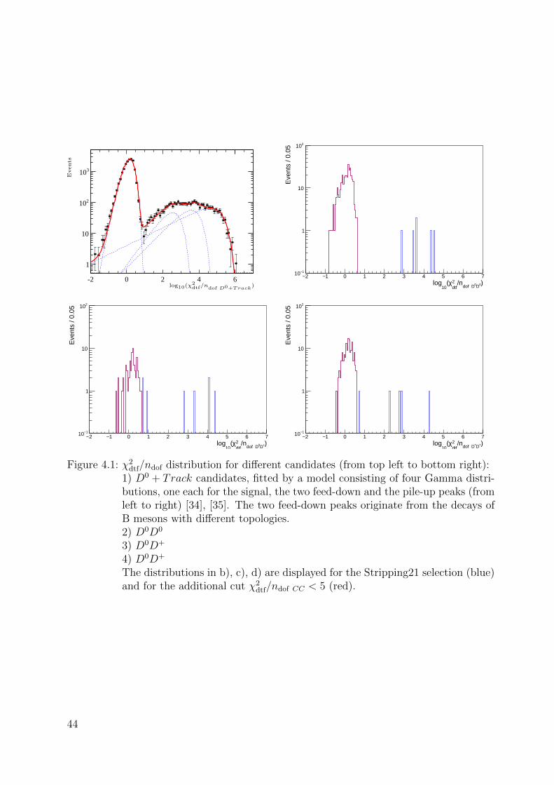
-2 0 2 4 6
1
10
210
310
log10(χ2dtf/ndof D0+Track
)
Events
)0D0dof D/n
dtf2χ(
10log
2− 1− 0 1 2 3 4 5 6 7
Eve
nts
/ 0.0
5
1−10
1
10
210
)+D0dof D/n
dtf2χ(
10log
2− 1− 0 1 2 3 4 5 6 7
Eve
nts
/ 0.0
5
1−10
1
10
210
)+D+dof D/ndtf2χ(
10log
2− 1− 0 1 2 3 4 5 6 7
Eve
nts
/ 0.0
5
1−10
1
10
210
Figure 4.1: χ2dtf/ndof distribution for different candidates (from top left to bottom right):
1) D0 + Track candidates, fitted by a model consisting of four Gamma distri-butions, one each for the signal, the two feed-down and the pile-up peaks (fromleft to right) [34], [35]. The two feed-down peaks originate from the decays ofB mesons with different topologies.2) D0D0
3) D0D+
4) D0D+
The distributions in b), c), d) are displayed for the Stripping21 selection (blue)and for the additional cut χ2
dtf/ndof CC < 5 (red).
44

4.3 Selected Candidates
This chapter illustrates the selected single open charm event candidates D0 and D+ modesD0 → K−π+, D+ → K−π+π+ and the selected double open charm event candidatesD0D0, D0D+ and D+D+ with corresponding decay modes D0D0 → 2 ·D0 → 2 · (K−π+),D0D+ → D0 +D+ → (K−π+) + (K−π+π+), D+D+ → 2 ·D+ → 2 · (K−π+π+).
The total number of events Ntot is extracted from the invariant mass distributions ofthe single and double open charm event candidates, MC , MCC , where C ∈ {D0, D+}, withfully applied event selection (see ch. 4.2.1). They are shown in Tab. 4.5, whereas thecorresponding invariant mass distributions are shown in Fig. 4.2 for D0 and D+, inFig. 4.3 for D0D0, D0D+ and D+D+ and in Fig. 4.4 for D0D0 and D+D−. Surprisingly noD0D− events were observed. So for this combination only the double open charm channelbut not the pair production channel is seen. This is considered a statistical fluctuation.Since Ntot for all double open charm event candidates is small, there is no need to considereven rarer candidates like D∗ 0, D∗+, D0
s , D+s .
Candidate Ntot, standard selection Ntot, (pT > 4 GeV, y > 2.25) selection
D0 96441 82087
D+ 59708 54138
D0D0 8 5
D0D+ 11 4
D+D+ 3 1
D0D0 79 21
D0D− 0 0
D+D− 48 25
Table 4.5: The total number of events for the single open charm, double open charm andopen charm pair production event candidates. The standard selection is theselection applied in chapter 4.2.1, the (pT > 4 GeV, y > 2.25) selection is theone according to chapter C (see also chapter 4.6).
45

[GeV]0DM1.82 1.83 1.84 1.85 1.86 1.87 1.88 1.89 1.9 1.91 1.92
Eve
nts
/ (0.
002
GeV
)
0
2000
4000
6000
8000
10000
[GeV]+DM1.82 1.83 1.84 1.85 1.86 1.87 1.88 1.89 1.9 1.91 1.92
Eve
nts
/ (0.
002
GeV
)
0
1000
2000
3000
4000
5000
6000
Figure 4.2: Invariant mass distributions of the single open charm event candidates D0 (left)and D+ (right).
46

[GeV]10
DM1.82 1.83 1.84 1.85 1.86 1.87 1.88 1.89 1.9 1.911.92
[GeV]20D
M
1.821.83
1.841.85
1.861.87
1.881.89
1.91.91
1.92
Eve
nts
/ (0.
005
* 0.
005
GeV
)
0
0.2
0.4
0.6
0.8
1
[GeV]10D
M1.82 1.83 1.84 1.85 1.86 1.87 1.88 1.89 1.9 1.91 1.92
[GeV
]20
DM
1.82
1.83
1.84
1.85
1.86
1.87
1.88
1.89
1.9
1.91
1.92
Eve
nts
/ (0.
005
* 0.
005
GeV
)
0
0.1
0.2
0.3
0.4
0.5
0.6
0.7
0.8
0.9
1
[GeV]10
DM1.82 1.83 1.84 1.85 1.86 1.87 1.88 1.89 1.9 1.911.92
[GeV]2+D
M
1.821.83
1.841.85
1.861.87
1.881.89
1.91.91
1.92
Eve
nts
/ (0.
005
* 0.
005
GeV
)
00.20.40.60.8
11.21.41.61.8
22.2
[GeV]10D
M1.82 1.83 1.84 1.85 1.86 1.87 1.88 1.89 1.9 1.91 1.92
[GeV
]2+
DM
1.82
1.83
1.84
1.85
1.86
1.87
1.88
1.89
1.9
1.91
1.92
Eve
nts
/ (0.
005
* 0.
005
GeV
)
0
0.2
0.4
0.6
0.8
1
1.2
1.4
1.6
1.8
2
[GeV]1+
DM1.82 1.83 1.84 1.85 1.86 1.87 1.88 1.89 1.9 1.911.92
[GeV]2+D
M
1.821.83
1.841.85
1.861.87
1.881.89
1.91.91
1.92
Eve
nts
/ (0.
005
* 0.
005
GeV
)
0
0.2
0.4
0.6
0.8
1
[GeV]1+DM
1.82 1.83 1.84 1.85 1.86 1.87 1.88 1.89 1.9 1.91 1.92
[GeV
]2+
DM
1.82
1.83
1.84
1.85
1.86
1.87
1.88
1.89
1.9
1.91
1.92
Eve
nts
/ (0.
005
* 0.
005
GeV
)
0
0.1
0.2
0.3
0.4
0.5
0.6
0.7
0.8
0.9
1
Figure 4.3: Invariant mass distributions for the double open charm event candidates D0D0
(1st row), D0D+ (2nd row) and D+D+ (3rd row).
47

[GeV]10
DM1.82 1.83 1.84 1.85 1.86 1.87 1.88 1.89 1.9 1.911.92
[GeV]20D
M
1.821.83
1.841.85
1.861.87
1.881.89
1.91.91
1.92
Eve
nts
/ (0.
005
* 0.
005
GeV
)
0
1
2
3
4
5
6
7
[GeV]10D
M1.82 1.83 1.84 1.85 1.86 1.87 1.88 1.89 1.9 1.91 1.92
[GeV
]20
DM
1.82
1.83
1.84
1.85
1.86
1.87
1.88
1.89
1.9
1.91
1.92
Eve
nts
/ (0.
005
* 0.
005
GeV
)
0
1
2
3
4
5
6
7
[GeV]1+
DM1.82 1.83 1.84 1.85 1.86 1.87 1.88 1.89 1.9 1.911.92
[GeV]2
-DM
1.821.83
1.841.85
1.861.87
1.881.89
1.91.91
1.92
Eve
nts
/ (0.
005
* 0.
005
GeV
)
0
1
2
3
4
5
[GeV]1+DM
1.82 1.83 1.84 1.85 1.86 1.87 1.88 1.89 1.9 1.91 1.92
[GeV
]2-
DM
1.82
1.83
1.84
1.85
1.86
1.87
1.88
1.89
1.9
1.91
1.92
Eve
nts
/ (0.
005
* 0.
005
GeV
)
0
0.5
1
1.5
2
2.5
3
3.5
4
4.5
5
Figure 4.4: Invariant mass distributions for the charm pair production event candidatesD0D0 (1st row) and D+D− (2nd row). No event candidates are observed forthe case D0D−.
48

4.4 Invariant Mass Fits
The number of signal events is extracted by unbinned maximum likelihood fits to theinvariant mass distributions of the single and double open charm event candidates, MC andMCC , where C ∈ {D0, D+} using the RooFit v3.60 package within the ROOT frameworkv6.06.02 [36]. The fits give an estimate of the normalization parameter for the signal,which is the number of signal events. The quality of this estimate depends on the chosenfit model. Three models are tested to find the one, which gives the best estimate. Thesimplest option for a model is given by a Gaussian probability density function (PDF), thesecond by a Bukin PDF and the third by a Double Crystal Ball PDF. Each model consistsof a signal component S(M), given by the three options, and a background componentB(M), given by an Exponential PDF. In order to evaluate the quality of the fits, threegoodness of fit criteria are imposed. The first is the reduced χ2, χ2/ndof, the second theupper tail probability or upper p-value of the corresponding χ2 distribution, Pu(χ
2, ndof)and the third the distribution of the pull values pi (see ch. 3.1.2). In contrast to theGaussian PDF, the Bukin and Double Crystal Ball PDF can describe initial and finalstate radiation. The Gaussian model is used to gauge the pull distributions for a wrongmodel. Since the layout for the construction of the fit models for MC is different than forMCC , the invariant mass fits for the two open charm event cases are separated, providinga better overview.
Single Open Charm Event CandidatesThe invariant mass distributions for the single open charm event candidates D0, D+, MD0 ,MD+ , are one dimensional. Therefore the fit model F with its components S(M), B(M)is also one dimensional. The functional form of the fit model is:
F (S(M), B(M)) = NS · S(M) +NB ·B(M) ,
where M : invariant mass of the single open charm
event candidates D0, D+
S(M), NS : signal component with its normalization parameter
(number of signal events)
B(M), NB : background component with its normalization parameter
(number of background events) .
(4.6)
49

The functional form of the signal component S(M) is given according to the three options:
1) Gaussian PDF:
S(M) = Gauss(M ;µ, σ)
= exp
(−(M − µ)2
2σ2
),
where µ : peak position, i.e. expectation value of the PDF
σ : peak width, i.e. standard deviation defined by σ =FWHM
2√
2 ln (2).
(4.7)
2) Bukin PDF:
S(M) = Bukin(M ;µ, σ, ξ, ρl, ρr)
=
12
exp
( √2 ln (2) ξ
√ξ2+1 (M−m1)
σ(√
ξ2+1−ξ)2
ln(√
ξ2+1+ξ) + ρl
(M−m1
µ−m1
)2)
, M < m1
exp
(− ln (2)
(ln
(1 + 2ξ
√ξ2+1 M−µ
σ√
2 ln 2
)ln
(1+2ξ2−2ξ
√ξ2+1
))2)
, m1 < M < m2
12
exp
( √2 ln (2) ξ
√ξ2+1 (M−m2)
σ(√
ξ2+1−ξ)2
ln(√
ξ2+1+ξ) + ρr
(M−m2
µ−m2
)2)
, M > m2
,
where µ : peak position, i.e. expectation value of the PDF
σ : peak width, i.e. standard deviation defined by σ =FWHM
2√
2 ln (2)
ξ : asymmetry parameter
ρl, ρr : left and right tail parameters
m1,2 = µ + σ√
2 ln (2)
(ξ√ξ2 + 1
∓ 1
).
(4.8)
50
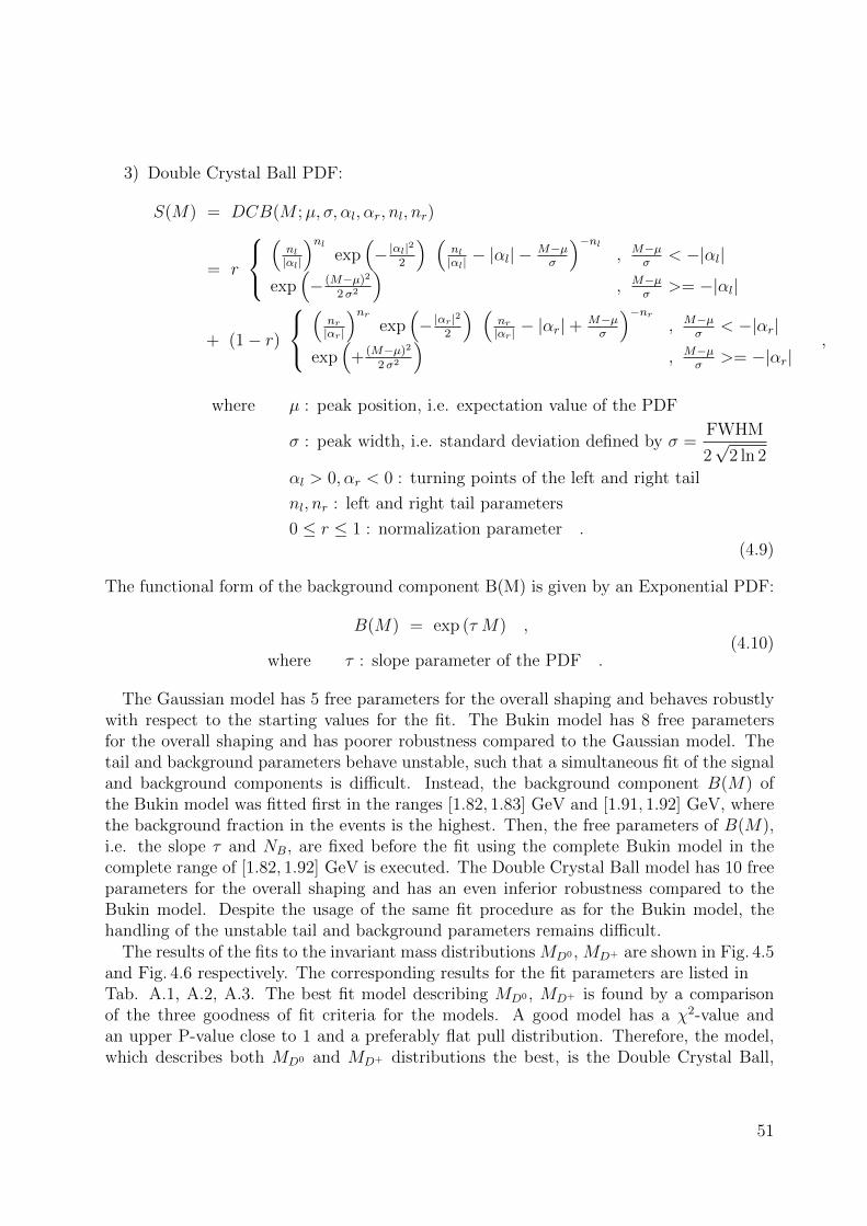
3) Double Crystal Ball PDF:
S(M) = DCB(M ;µ, σ, αl, αr, nl, nr)
= r
(nl|αl|
)nlexp
(− |αl|
2
2
) (nl|αl|− |αl| − M−µ
σ
)−nl, M−µ
σ< −|αl|
exp(− (M−µ)2
2σ2
), M−µ
σ>= −|αl|
+ (1− r)
(nr|αr|
)nrexp
(− |αr|
2
2
) (nr|αr| − |αr|+
M−µσ
)−nr, M−µ
σ< −|αr|
exp(
+ (M−µ)2
2σ2
), M−µ
σ>= −|αr|
,
where µ : peak position, i.e. expectation value of the PDF
σ : peak width, i.e. standard deviation defined by σ =FWHM
2√
2 ln 2
αl > 0, αr < 0 : turning points of the left and right tail
nl, nr : left and right tail parameters
0 ≤ r ≤ 1 : normalization parameter .(4.9)
The functional form of the background component B(M) is given by an Exponential PDF:
B(M) = exp (τ M) ,
where τ : slope parameter of the PDF .(4.10)
The Gaussian model has 5 free parameters for the overall shaping and behaves robustlywith respect to the starting values for the fit. The Bukin model has 8 free parametersfor the overall shaping and has poorer robustness compared to the Gaussian model. Thetail and background parameters behave unstable, such that a simultaneous fit of the signaland background components is difficult. Instead, the background component B(M) ofthe Bukin model was fitted first in the ranges [1.82, 1.83] GeV and [1.91, 1.92] GeV, wherethe background fraction in the events is the highest. Then, the free parameters of B(M),i.e. the slope τ and NB, are fixed before the fit using the complete Bukin model in thecomplete range of [1.82, 1.92] GeV is executed. The Double Crystal Ball model has 10 freeparameters for the overall shaping and has an even inferior robustness compared to theBukin model. Despite the usage of the same fit procedure as for the Bukin model, thehandling of the unstable tail and background parameters remains difficult.
The results of the fits to the invariant mass distributions MD0 , MD+ are shown in Fig. 4.5and Fig. 4.6 respectively. The corresponding results for the fit parameters are listed inTab. A.1, A.2, A.3. The best fit model describing MD0 , MD+ is found by a comparisonof the three goodness of fit criteria for the models. A good model has a χ2-value andan upper P-value close to 1 and a preferably flat pull distribution. Therefore, the model,which describes both MD0 and MD+ distributions the best, is the Double Crystal Ball,
51

closely followed by the Bukin model. The fit quality of the Gaussian model is inferior tothe Bukin and Double Crystal Ball models, also clearly visible by eye. This is expected,since the Gaussian model neglects the tails of the invariant mass distributions, which areknown to be present in LHCb data. Since the Double Crystal Ball model has two morefree parameters than the Bukin model, it is in principle expected to describe the invariantmass distribution better. The direct comparison of the pull distributions of the Bukin andDouble Crystal Ball models in Fig. 4.7 reveals, that the Bukin model has more difficultiesto describe the lower tail of the invariant mass distributions than the Double Crystal Ballmodel, whereas both models describe the upper tail nearly equivalently good. The smalldifference in the fit quality of these two models can therefore be caused by the differencein the amount of free parameters. The disagreement to the previous analysis can also becaused by the smaller available center of mass energy
√s and total number of events of
the invariant mass distributions. It is concluded, that the Double Crystal Ball model doesnot describe the invariant mass distributions significantly better than the Bukin model.Not enough justification is found in order abandon the commonly used Bukin model inpreference of the Double Crystal Ball model, i.e. the difference in the fit quality of thetwo models is so small, that it is considered irrelevant in the further analysis. Therefore,the Bukin model is chosen to describe the invariant mass of the single open charm eventcandidates.
52
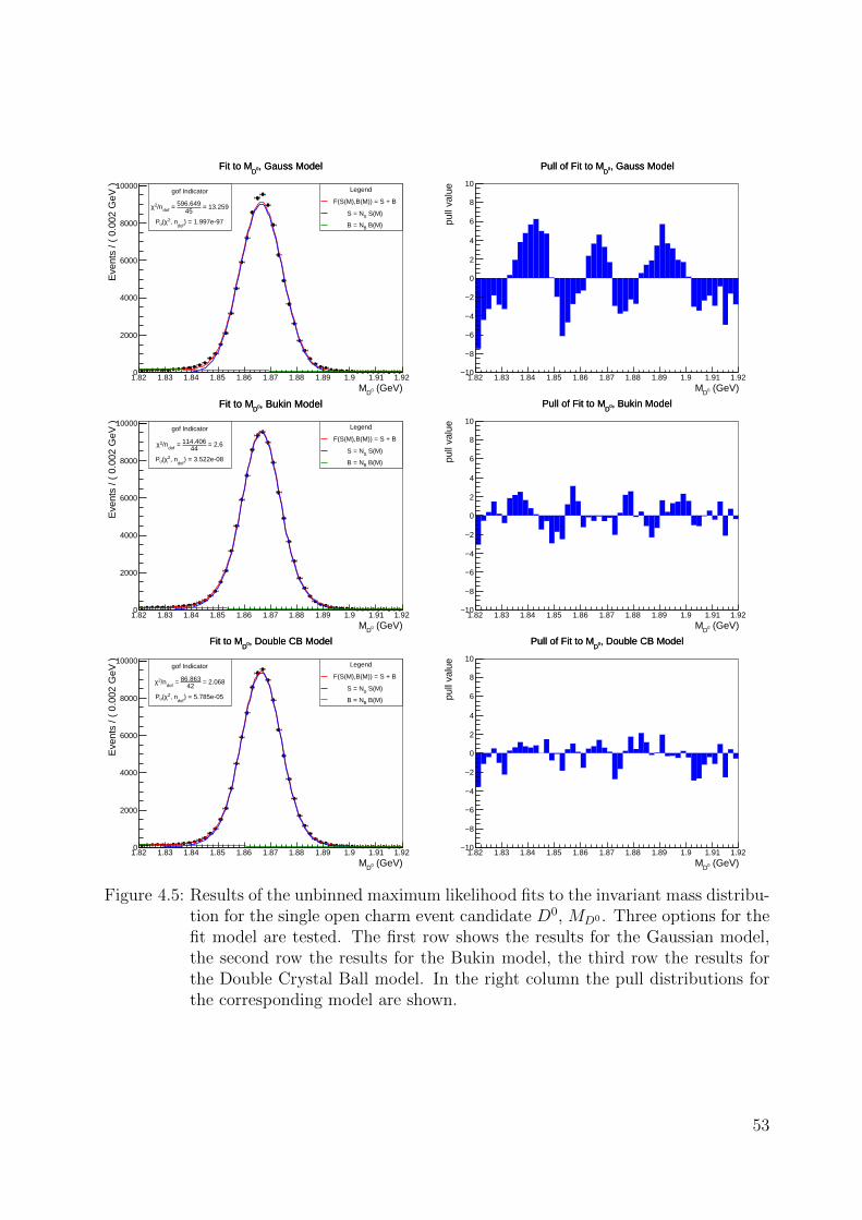
(GeV)0DM1.82 1.83 1.84 1.85 1.86 1.87 1.88 1.89 1.9 1.91 1.92
Eve
nts
/ ( 0
.002
GeV
)
0
2000
4000
6000
8000
10000
, Gauss Model0DFit to M
gof Indicator
= 13.25945
596.649 = dof/n2χ
) = 1.997e-97dof
, n2χ(uP
Legend
F(S(M),B(M)) = S + B
S(M)SS = N
B(M)BB = N
, Gauss Model0DFit to M
(GeV)0DM1.82 1.83 1.84 1.85 1.86 1.87 1.88 1.89 1.9 1.91 1.92
pull
valu
e
10−
8−
6−
4−
2−
0
2
4
6
8
10
, Gauss Model0DPull of Fit to M , Gauss Model0DPull of Fit to M
(GeV)0DM1.82 1.83 1.84 1.85 1.86 1.87 1.88 1.89 1.9 1.91 1.92
Eve
nts
/ ( 0
.002
GeV
)
0
2000
4000
6000
8000
10000
, Bukin Model0DFit to M
gof Indicator
= 2.644
114.406 = dof
/n2χ
) = 3.522e-08dof
, n2χ(uP
Legend
F(S(M),B(M)) = S + B
S(M)SS = N
B(M)BB = N
, Bukin Model0DFit to M
(GeV)0DM1.82 1.83 1.84 1.85 1.86 1.87 1.88 1.89 1.9 1.91 1.92
pull
valu
e
10−
8−
6−
4−
2−
0
2
4
6
8
10
, Bukin Model0DPull of Fit to M , Bukin Model0DPull of Fit to M
(GeV)0DM1.82 1.83 1.84 1.85 1.86 1.87 1.88 1.89 1.9 1.91 1.92
Eve
nts
/ ( 0
.002
GeV
)
0
2000
4000
6000
8000
10000
, Double CB Model0DFit to M
gof Indicator
= 2.06842
86.863 = dof
/n2χ
) = 5.785e-05dof
, n2χ(uP
Legend
F(S(M),B(M)) = S + B
S(M)SS = N
B(M)BB = N
, Double CB Model0DFit to M
(GeV)0DM1.82 1.83 1.84 1.85 1.86 1.87 1.88 1.89 1.9 1.91 1.92
pull
valu
e
10−
8−
6−
4−
2−
0
2
4
6
8
10
, Double CB Model0DPull of Fit to M , Double CB Model0DPull of Fit to M
Figure 4.5: Results of the unbinned maximum likelihood fits to the invariant mass distribu-tion for the single open charm event candidate D0, MD0 . Three options for thefit model are tested. The first row shows the results for the Gaussian model,the second row the results for the Bukin model, the third row the results forthe Double Crystal Ball model. In the right column the pull distributions forthe corresponding model are shown.
53

(GeV)+DM1.82 1.83 1.84 1.85 1.86 1.87 1.88 1.89 1.9 1.91 1.92
Eve
nts
/ ( 0
.002
GeV
)
0
1000
2000
3000
4000
5000
6000
, Gauss Model+DFit to M
gof Indicator
= 13.74145
618.328 = dof/n2χ
) = 8.413e-102dof
, n2χ(uP
Legend
F(S(M),B(M)) = S + B
S(M)SS = N
B(M)BB = N
, Gauss Model+DFit to M
(GeV)+DM1.82 1.83 1.84 1.85 1.86 1.87 1.88 1.89 1.9 1.91 1.92
pull
valu
e
10−
8−
6−
4−
2−
0
2
4
6
8
10
, Gauss Model+DPull of Fit to M , Gauss Model+DPull of Fit to M
(GeV)+DM1.82 1.83 1.84 1.85 1.86 1.87 1.88 1.89 1.9 1.91 1.92
Eve
nts
/ ( 0
.002
GeV
)
0
1000
2000
3000
4000
5000
6000
, Bukin Model+DFit to M
gof Indicator
= 2.83744
124.81 = dof
/n2χ
) = 1.154e-09dof
, n2χ(uP
Legend
F(S(M),B(M)) = S + B
S(M)SS = N
B(M)BB = N
, Bukin Model+DFit to M
(GeV)+DM1.82 1.83 1.84 1.85 1.86 1.87 1.88 1.89 1.9 1.91 1.92
pull
valu
e
10−
8−
6−
4−
2−
0
2
4
6
8
10
, Bukin Model+DPull of Fit to M , Bukin Model+DPull of Fit to M
(GeV)+DM1.82 1.83 1.84 1.85 1.86 1.87 1.88 1.89 1.9 1.91 1.92
Eve
nts
/ ( 0
.002
GeV
)
0
1000
2000
3000
4000
5000
6000
, Double CB Model+DFit to M
gof Indicator
= 1.54742
64.955 = dof
/n2χ
) = 0.013dof
, n2χ(uP
Legend
F(S(M),B(M)) = S + B
S(M)SS = N
B(M)BB = N
, Double CB Model+DFit to M
(GeV)+DM1.82 1.83 1.84 1.85 1.86 1.87 1.88 1.89 1.9 1.91 1.92
pull
valu
e
10−
8−
6−
4−
2−
0
2
4
6
8
10
, Double CB Model+DPull of Fit to M , Double CB Model+DPull of Fit to M
Figure 4.6: Results of the unbinned maximum likelihood fits to the invariant mass distri-bution for the single open charm event candidate D+, MD+ . Three options forthe fit model are tested. The first row shows the results for the Gaussian model,the second row the results for the Bukin model, the third row the results forthe Double Crystal Ball model. In the right column the pull distributions forthe corresponding model are shown.
54

(GeV)0DM1.82 1.83 1.84 1.85 1.86 1.87 1.88 1.89 1.9 1.91 1.92
pull
valu
e
4−
3−
2−
1−
0
1
2
3
4
, Bukin vs. Double CB Model0DPull of Fit to M
Legend
Bukin Model
Double CB Model
, Bukin vs. Double CB Model0DPull of Fit to M
(GeV)+DM1.82 1.83 1.84 1.85 1.86 1.87 1.88 1.89 1.9 1.91 1.92
pull
valu
e
4−
3−
2−
1−
0
1
2
3
4
, Bukin vs. Double CB Model+DPull of Fit to M
Legend
Bukin Model
Double CB Model
, Bukin vs. Double CB Model+DPull of Fit to M
Figure 4.7: The pull distributions of the maximum likelihood fits to the invariant massdistributions MD0 (left) and MD+ (right) for the Bukin model (blue) and theDouble Crystal Ball model (red) in direct comparison.
Double Open Charm resp. Open Charm Pair Production Event CandidatesDue to the low total number of events in the double charm meson cases D0D0, D0D+,D+D+, the fit model for the two dimensional mass distributions is constructed based onthe ones used for the single charm meson cases. All shape related fit parameters for thesignal were determined on the single open charm sample and then fixed and used for thedouble open charm sample, whereas the fit parameters for the background shape are leftfree. In order to increase the total number of events of the mass distributions MCC , thedouble open charm production and pair production samples are temporarily merged, i.e.D0D0 := {D0D0 ∪D0D0}, D0D+ := {D0D+ ∪D0D−} and D+D+ := {D+D+ ∪D+D−}.These samples are separated from each other in chapter 4.5. For the D0D0 and D+D+
cases, the D0, D+ candidates are assigned randomly to be first or second. The notationMC1C2 originates only from the definition, that MC1 is related to the x-axis and MC2 isrelated to the y-axis of the two dimensional invariant mass distributions. The functionalform of the fit model is:
55

F (S1(MC1), S2(MC2), B1(MC1), B2(MC2))
= NS1S2 S1(MC1) S2(MC2) + NB1B2 B1(MC1) B2(MC2)
+ NS1B2 S1(MC1) B2(MC2) + NS2B1 S2(MC2) B1(MC1) ,
where MCl , Cl ∈ {D0, D+} , l ∈ {1, 2} :
invariant mass of the single open charm components to the corresponding
double open charm event candidates (including open charm pair production)
{D0D0 ∪D0D0}, {D0D+ ∪D0D−} and {D+D+ ∪D+D−}
Sl , l ∈ {1, 2} : signal component of the single charm components
to the corresponding double open charm event candidates
(including open charm pair production)
Bl , l ∈ {1, 2} : background component of the single open charm components
to the corresponding double open charm event candidates
(including open charm pair production)
NS1S2 , NS1B2 , NS2B1 , NB1B2 :
normalization parameters for the four components of the fit model .(4.11)
The functional form of Sl(MCl), Bl(MCl), where Cl ∈ {D0, D+} , l ∈ {1, 2} is described inequation 4.6.
56
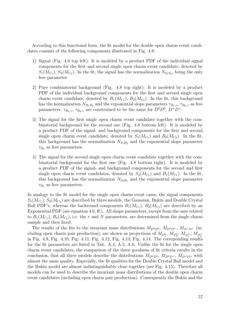
According to this functional form, the fit model for the double open charm event candi-dates consists of the following components illustrated in Fig. 4.8:
1) Signal (Fig. 4.8 top left): It is modeled by a product PDF of the individual signalcomponents for the first and second single open charm event candidate, denoted byS1(MC1), S2(MC2). In the fit, the signal has the normalization NS1S2 , being the onlyfree parameter.
2) Pure combinatorial background (Fig. 4.8 top right): It is modeled by a productPDF of the individual background components for the first and second single opencharm event candidate, denoted by B1(MC1), B2(MC2). In the fit, this backgroundhas the normalization NB1B2 and the exponential slope parameters τB1, c, τB2, c as freeparameters. τB1, c, τB2, c are constrained to be the same for D0D0, D+D+.
3) The signal for the first single open charm event candidate together with the com-binatorial background for the second one (Fig. 4.8 bottom left). It is modeled bya product PDF of the signal- and background components for the first and secondsingle open charm event candidate, denoted by S1(MC1) and B2(MC2). In the fit,this background has the normalization NS1B2 and the exponential slope parameterτB2 as free parameters.
4) The signal for the second single open charm event candidate together with the com-binatorial background for the first one (Fig. 4.8 bottom right). It is modeled bya product PDF of the signal- and background components for the second and firstsingle open charm event candidates, denoted by S2(MC2) and B1(MC1). In the fit,this background has the normalization NS2B1 and the exponential slope parameterτB1 as free parameters.
In analogy to the fit model for the single open charm event cases, the signal componentsS1(MC1), S2(MC2) are described by three models, the Gaussian, Bukin and Double CrystalBall PDF’s, whereas the backround components B1(MC1), B2(MC2) are described by anExponential PDF (see equation 4.6, ff.). All shape parameters, except from the ones relatedto B1(MC1), B2(MC2), i.e. the τ and N parameters, are determined from the single charmsample and then fixed.
The results of the fits to the invariant mass distributions MD0D0 , MD0D+ , MD+D+ (in-cluding open charm pair production), are shown as projections of MD0
1, MD0
2, MD+
1, MD+
2
in Fig. 4.9, Fig. 4.10, Fig. 4.11, Fig. 4.12, Fig. 4.13, Fig. 4.14. The correponding resultsfor the fit parameters are listed in Tab. A.4, A.5, A.6. Unlike the fit for the single opencharm event candidates, the comparison of the three goodness of fit criteria results in theconclusion, that all three models describe the distributions MD0D0 , MD0D+ , MD+D+ withalmost the same quality. Especially, the fit qualities for the Double Crystal Ball model andthe Bukin model are almost indistinguishably close together (see Fig. 4.15). Therefore allmodels can be used to describe the invariant mass distributions of the double open charmevent candidates (including open charm pair production). Consequently the Bukin and the
57
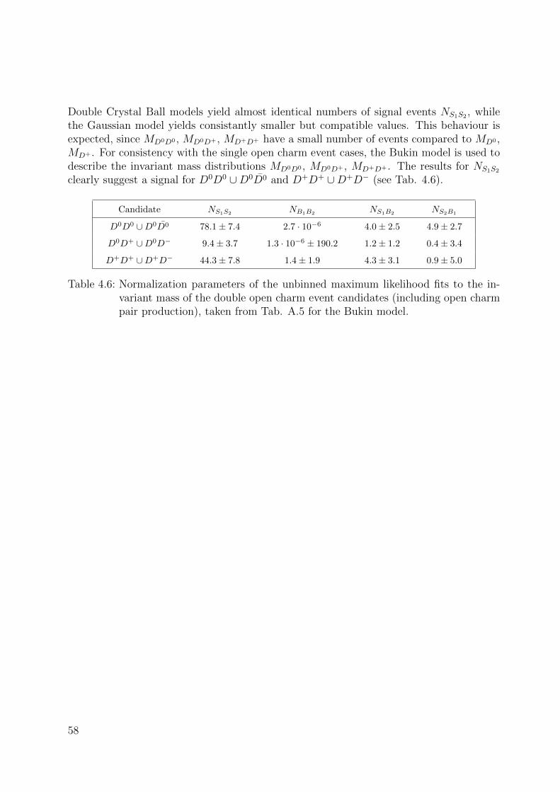
Double Crystal Ball models yield almost identical numbers of signal events NS1S2 , whilethe Gaussian model yields consistantly smaller but compatible values. This behaviour isexpected, since MD0D0 , MD0D+ , MD+D+ have a small number of events compared to MD0 ,MD+ . For consistency with the single open charm event cases, the Bukin model is used todescribe the invariant mass distributions MD0D0 , MD0D+ , MD+D+ . The results for NS1S2
clearly suggest a signal for D0D0 ∪D0D0 and D+D+ ∪D+D− (see Tab. 4.6).
Candidate NS1S2 NB1B2 NS1B2 NS2B1
D0D0 ∪D0D0 78.1± 7.4 2.7 · 10−6 4.0± 2.5 4.9± 2.7
D0D+ ∪D0D− 9.4± 3.7 1.3 · 10−6 ± 190.2 1.2± 1.2 0.4± 3.4
D+D+ ∪D+D− 44.3± 7.8 1.4± 1.9 4.3± 3.1 0.9± 5.0
Table 4.6: Normalization parameters of the unbinned maximum likelihood fits to the in-variant mass of the double open charm event candidates (including open charmpair production), taken from Tab. A.5 for the Bukin model.
58

(GeV)10
DM1.82 1.83 1.84 1.85 1.86 1.87 1.88 1.89 1.9 1.911.92
(GeV)2
0DM
1.821.83
1.841.85
1.861.87
1.881.89
1.91.91
1.92
Eve
nts
/ ( 0
.005
GeV
x 0
.005
GeV
)
0
1
2
3
4
5
2 Sig
1 Sig
2S1SN2
Sig1
Sig2S1SN
(GeV)10
DM1.82 1.83 1.84 1.85 1.86 1.87 1.88 1.89 1.9 1.911.92
(GeV)2
0DM
1.821.83
1.841.85
1.861.87
1.881.89
1.91.91
1.92
Eve
nts
/ ( 0
.005
GeV
x 0
.005
GeV
)
4
5
6
7
8
9
10
11
9−10×
2 Bkg
1 Bkg
2B1BN2
Bkg1
Bkg2B1BN
(GeV)10
DM1.82 1.83 1.84 1.85 1.86 1.87 1.88 1.89 1.9 1.911.92
(GeV)2
0DM
1.821.83
1.841.85
1.861.87
1.881.89
1.91.91
1.92
Eve
nts
/ ( 0
.005
GeV
x 0
.005
GeV
)
0
0.01
0.02
0.03
0.04
0.05
0.06
0.07
0.08
2 Bkg
1 Sig
2B1SN2
Bkg1
Sig2B1SN
(GeV)10
DM1.82 1.83 1.84 1.85 1.86 1.87 1.88 1.89 1.9 1.911.92
(GeV)2
0DM
1.821.83
1.841.85
1.861.87
1.881.89
1.91.91
1.92
Eve
nts
/ ( 0
.005
GeV
x 0
.005
GeV
)
00.010.020.030.040.050.060.070.080.09
1 Bkg
2 Sig
1B2SN1
Bkg2
Sig1B2SN
Figure 4.8: Graphical illustration of the functional form of the fit model for the doubleopen charm event candidates D0D0 (including open charm pair production).The four images show the four components of the fit model: NS1S2 Sig1 Sig2
(top left), NB1B2 Bkg1 Bkg2 (top right), NS1B2 Sig1 Bkg2 (bottom left) andNS2B1 Sig2 Bkg1 (bottom right).
59
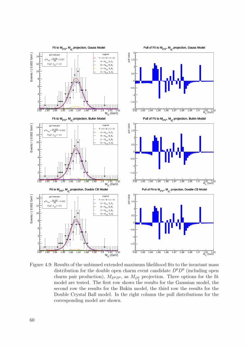
(GeV)10D
M1.82 1.83 1.84 1.85 1.86 1.87 1.88 1.89 1.9 1.91 1.92
Eve
nts
/ ( 0
.002
GeV
)
0
2
4
6
8
10
12
14
projection, Gauss Model10D
, M0D0DFit to M
gof Indicator
= 0.32744
14.39 = dof
/n2χ
) = 1.0dof
, n2χ(uP
Legend
F = A + B + C + D
2 S1 S2S1SA = N
2 B1 B2B1BB = N
2 B1 S2B1SC = N
1 B2 S1B2SD = N
projection, Gauss Model10D
, M0D0DFit to M
(GeV)10D
M1.82 1.83 1.84 1.85 1.86 1.87 1.88 1.89 1.9 1.91 1.92
pull
valu
e
2−
1.5−
1−
0.5−
0
0.5
1
1.5
2
projection, Gauss Model10D
, M0D0DPull of Fit to M projection, Gauss Model
10D
, M0D0DPull of Fit to M
(GeV)10D
M1.82 1.83 1.84 1.85 1.86 1.87 1.88 1.89 1.9 1.91 1.92
Eve
nts
/ ( 0
.002
GeV
)
0
2
4
6
8
10
12
14
projection, Bukin Model10D
, M0D0DFit to M
gof Indicator
= 0.32344
14.209 = dof
/n2χ
) = 1.0dof
, n2χ(uP
Legend
F = A + B + C + D
2 S1 S2S1SA = N
2 B1 B2B1BB = N
2 B1 S2B1SC = N
1 B2 S1B2SD = N
projection, Bukin Model10D
, M0D0DFit to M
(GeV)10D
M1.82 1.83 1.84 1.85 1.86 1.87 1.88 1.89 1.9 1.91 1.92
pull
valu
e
2−
1.5−
1−
0.5−
0
0.5
1
1.5
2
projection, Bukin Model10D
, M0D0DPull of Fit to M projection, Bukin Model
10D
, M0D0DPull of Fit to M
(GeV)10D
M1.82 1.83 1.84 1.85 1.86 1.87 1.88 1.89 1.9 1.91 1.92
Eve
nts
/ ( 0
.002
GeV
)
0
2
4
6
8
10
12
14
projection, Double CB Model10D
, M0D0DFit to M
gof Indicator
= 0.32344
14.197 = dof
/n2χ
) = 1.0dof
, n2χ(uP
Legend
F = A + B + C + D
2 S1 S2S1SA = N
2 B1 B2B1BB = N
2 B1 S2B1SC = N
1 B2 S1B2SD = N
projection, Double CB Model10D
, M0D0DFit to M
(GeV)10D
M1.82 1.83 1.84 1.85 1.86 1.87 1.88 1.89 1.9 1.91 1.92
pull
valu
e
2−
1.5−
1−
0.5−
0
0.5
1
1.5
2
projection, Double CB Model10D
, M0D0DPull of Fit to M projection, Double CB Model
10D
, M0D0DPull of Fit to M
Figure 4.9: Results of the unbinned extended maximum likelihood fits to the invariant massdistribution for the double open charm event candidate D0D0 (including opencharm pair production), MD0D0 , as MD0
1projection. Three options for the fit
model are tested. The first row shows the results for the Gaussian model, thesecond row the results for the Bukin model, the third row the results for theDouble Crystal Ball model. In the right column the pull distributions for thecorresponding model are shown.
60

(GeV)20D
M1.82 1.83 1.84 1.85 1.86 1.87 1.88 1.89 1.9 1.91 1.92
Eve
nts
/ ( 0
.002
GeV
)
0
2
4
6
8
10
12
14
16
projection, Gauss Model20D
, M0D0DFit to M
gof Indicator
= 0.47444
20.844 = dof
/n2χ
) = 0.999dof
, n2χ(uP
Legend
F = A + B + C + D
2 S1 S2S1SA = N
2 B1 B2B1BB = N
2 B1 S2B1SC = N
1 B2 S1B2SD = N
projection, Gauss Model20D
, M0D0DFit to M
(GeV)20D
M1.82 1.83 1.84 1.85 1.86 1.87 1.88 1.89 1.9 1.91 1.92
pull
valu
e
2−
1.5−
1−
0.5−
0
0.5
1
1.5
2
projection, Gauss Model20D
, M0D0DPull of Fit to M projection, Gauss Model
20D
, M0D0DPull of Fit to M
(GeV)20D
M1.82 1.83 1.84 1.85 1.86 1.87 1.88 1.89 1.9 1.91 1.92
Eve
nts
/ ( 0
.002
GeV
)
0
2
4
6
8
10
12
14
16
projection, Bukin Model20D
, M0D0DFit to M
gof Indicator
= 0.46144
20.28 = dof
/n2χ
) = 0.999dof
, n2χ(uP
Legend
F = A + B + C + D
2 S1 S2S1SA = N
2 B1 B2B1BB = N
2 B1 S2B1SC = N
1 B2 S1B2SD = N
projection, Bukin Model20D
, M0D0DFit to M
(GeV)20D
M1.82 1.83 1.84 1.85 1.86 1.87 1.88 1.89 1.9 1.91 1.92
pull
valu
e
2−
1.5−
1−
0.5−
0
0.5
1
1.5
2
projection, Bukin Model20D
, M0D0DPull of Fit to M projection, Bukin Model
20D
, M0D0DPull of Fit to M
(GeV)20D
M1.82 1.83 1.84 1.85 1.86 1.87 1.88 1.89 1.9 1.91 1.92
Eve
nts
/ ( 0
.002
GeV
)
0
2
4
6
8
10
12
14
16
projection, Double CB Model20D
, M0D0DFit to M
gof Indicator
= 0.4644
20.224 = dof
/n2χ
) = 0.999dof
, n2χ(uP
Legend
F = A + B + C + D
2 S1 S2S1SA = N
2 B1 B2B1BB = N
2 B1 S2B1SC = N
1 B2 S1B2SD = N
projection, Double CB Model20D
, M0D0DFit to M
(GeV)20D
M1.82 1.83 1.84 1.85 1.86 1.87 1.88 1.89 1.9 1.91 1.92
pull
valu
e
2−
1.5−
1−
0.5−
0
0.5
1
1.5
2
projection, Double CB Model20D
, M0D0DPull of Fit to M projection, Double CB Model
20D
, M0D0DPull of Fit to M
Figure 4.10: Results of the unbinned extended maximum likelihood fits to the invariantmass distribution for the double open charm event candidate D0D0, MD0D0
(including open charm pair production), as MD02
projection. Three optionsfor the fit model are tested. The first row shows the results for the Gaus-sian model, the second row the results for the Bukin model, the third rowthe results for the Double Crystal Ball model. In the right column the pulldistributions for the corresponding model are shown.
61

(GeV)10D
M1.82 1.83 1.84 1.85 1.86 1.87 1.88 1.89 1.9 1.91 1.92
Eve
nts
/ ( 0
.002
GeV
)
0
0.5
1
1.5
2
2.5
3
3.5
4
4.5
projection, Gauss Model10D
, M+D0DFit to M
gof Indicator
= 0.1942
7.983 = dof
/n2χ
) = 1.0dof
, n2χ(uP
Legend
F = A + B + C + D
2 S1 S2S1SA = N
2 B1 B2B1BB = N
2 B1 S2B1SC = N
1 B2 S1B2SD = N
projection, Gauss Model10D
, M+D0DFit to M
(GeV)10D
M1.82 1.83 1.84 1.85 1.86 1.87 1.88 1.89 1.9 1.91 1.92
pull
valu
e
2−
1.5−
1−
0.5−
0
0.5
1
1.5
2
projection, Gauss Model10D
, M+D0DPull of Fit to M projection, Gauss Model
10D
, M+D0DPull of Fit to M
(GeV)10D
M1.82 1.83 1.84 1.85 1.86 1.87 1.88 1.89 1.9 1.91 1.92
Eve
nts
/ ( 0
.002
GeV
)
0
0.5
1
1.5
2
2.5
3
3.5
4
4.5
projection, Bukin Model10D
, M+D0DFit to M
gof Indicator
= 0.19142
8.027 = dof
/n2χ
) = 1.0dof
, n2χ(uP
Legend
F = A + B + C + D
2 S1 S2S1SA = N
2 B1 B2B1BB = N
2 B1 S2B1SC = N
1 B2 S1B2SD = N
projection, Bukin Model10D
, M+D0DFit to M
(GeV)10D
M1.82 1.83 1.84 1.85 1.86 1.87 1.88 1.89 1.9 1.91 1.92
pull
valu
e
2−
1.5−
1−
0.5−
0
0.5
1
1.5
2
projection, Bukin Model10D
, M+D0DPull of Fit to M projection, Bukin Model
10D
, M+D0DPull of Fit to M
(GeV)10D
M1.82 1.83 1.84 1.85 1.86 1.87 1.88 1.89 1.9 1.91 1.92
Eve
nts
/ ( 0
.002
GeV
)
0
0.5
1
1.5
2
2.5
3
3.5
4
4.5
projection, Double CB Model10D
, M+D0DFit to M
gof Indicator
= 0.19142
8.014 = dof
/n2χ
) = 1.0dof
, n2χ(uP
Legend
F = A + B + C + D
2 S1 S2S1SA = N
2 B1 B2B1BB = N
2 B1 S2B1SC = N
1 B2 S1B2SD = N
projection, Double CB Model10D
, M+D0DFit to M
(GeV)10D
M1.82 1.83 1.84 1.85 1.86 1.87 1.88 1.89 1.9 1.91 1.92
pull
valu
e
2−
1.5−
1−
0.5−
0
0.5
1
1.5
2
projection, Double CB Model10D
, M+D0DPull of Fit to M projection, Double CB Model
10D
, M+D0DPull of Fit to M
Figure 4.11: Results of the unbinned extended maximum likelihood fits to the invariantmass distribution for the double open charm event candidate D0D+ (includ-ing open charm pair production), MD0D+ , as MD0
1projection. Three options
for the fit model are tested. The first row shows the results for the Gaus-sian model, the second row the results for the Bukin model, the third rowthe results for the Double Crystal Ball model. In the right column the pulldistributions for the corresponding model are shown.
62
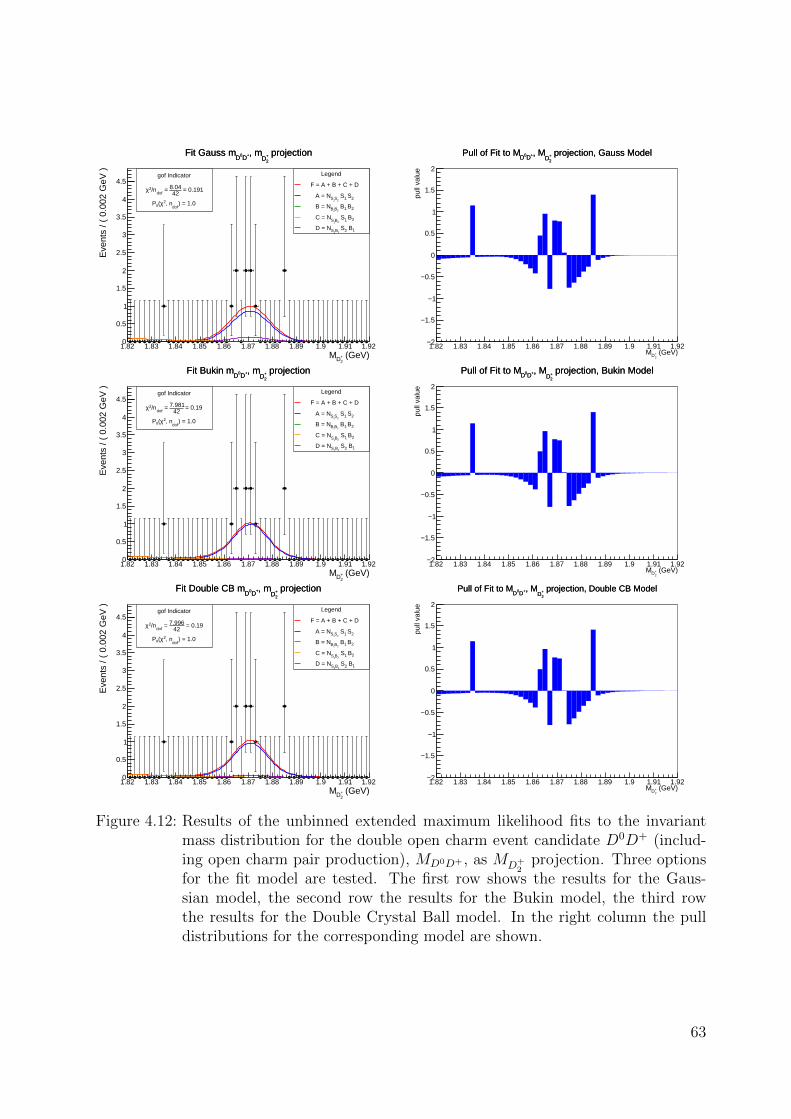
(GeV)2+DM
1.82 1.83 1.84 1.85 1.86 1.87 1.88 1.89 1.9 1.91 1.92
Eve
nts
/ ( 0
.002
GeV
)
0
0.5
1
1.5
2
2.5
3
3.5
4
4.5
projection2+D
, m+D0DFit Gauss m
gof Indicator
= 0.19142
8.04 = dof
/n2χ
) = 1.0dof
, n2χ(uP
Legend
F = A + B + C + D
2 S1 S2S1SA = N
2 B1 B2B1BB = N
2 B1 S2B1SC = N
1 B2 S1B2SD = N
projection2+D
, m+D0DFit Gauss m
(GeV)2+DM
1.82 1.83 1.84 1.85 1.86 1.87 1.88 1.89 1.9 1.91 1.92
pull
valu
e
2−
1.5−
1−
0.5−
0
0.5
1
1.5
2
projection, Gauss Model2+D
, M+D0DPull of Fit to M projection, Gauss Model
2+D
, M+D0DPull of Fit to M
(GeV)2+DM
1.82 1.83 1.84 1.85 1.86 1.87 1.88 1.89 1.9 1.91 1.92
Eve
nts
/ ( 0
.002
GeV
)
0
0.5
1
1.5
2
2.5
3
3.5
4
4.5
projection2+D
, m+D0DFit Bukin m
gof Indicator
= 0.1942
7.981 = dof
/n2χ
) = 1.0dof
, n2χ(uP
Legend
F = A + B + C + D
2 S1 S2S1SA = N
2 B1 B2B1BB = N
2 B1 S2B1SC = N
1 B2 S1B2SD = N
projection2+D
, m+D0DFit Bukin m
(GeV)2+DM
1.82 1.83 1.84 1.85 1.86 1.87 1.88 1.89 1.9 1.91 1.92
pull
valu
e
2−
1.5−
1−
0.5−
0
0.5
1
1.5
2
projection, Bukin Model2+D
, M+D0DPull of Fit to M projection, Bukin Model
2+D
, M+D0DPull of Fit to M
(GeV)2+DM
1.82 1.83 1.84 1.85 1.86 1.87 1.88 1.89 1.9 1.91 1.92
Eve
nts
/ ( 0
.002
GeV
)
0
0.5
1
1.5
2
2.5
3
3.5
4
4.5
projection2+D
, m+D0DFit Double CB m
gof Indicator
= 0.1942
7.996 = dof
/n2χ
) = 1.0dof
, n2χ(uP
Legend
F = A + B + C + D
2 S1 S2S1SA = N
2 B1 B2B1BB = N
2 B1 S2B1SC = N
1 B2 S1B2SD = N
projection2+D
, m+D0DFit Double CB m
(GeV)2+DM
1.82 1.83 1.84 1.85 1.86 1.87 1.88 1.89 1.9 1.91 1.92
pull
valu
e
2−
1.5−
1−
0.5−
0
0.5
1
1.5
2
projection, Double CB Model2+D
, M+D0DPull of Fit to M projection, Double CB Model
2+D
, M+D0DPull of Fit to M
Figure 4.12: Results of the unbinned extended maximum likelihood fits to the invariantmass distribution for the double open charm event candidate D0D+ (includ-ing open charm pair production), MD0D+ , as MD+
2projection. Three options
for the fit model are tested. The first row shows the results for the Gaus-sian model, the second row the results for the Bukin model, the third rowthe results for the Double Crystal Ball model. In the right column the pulldistributions for the corresponding model are shown.
63

(GeV)1+DM
1.82 1.83 1.84 1.85 1.86 1.87 1.88 1.89 1.9 1.91 1.92
Eve
nts
/ ( 0
.002
GeV
)
0
2
4
6
8
10
projection1+D
, m+D+DFit Gauss m
gof Indicator
= 0.53844
23.684 = dof
/n2χ
) = 0.995dof
, n2χ(uP
Legend
F = A + B + C + D
2 S1 S2S1SA = N
2 B1 B2B1BB = N
2 B1 S2B1SC = N
1 B2 S1B2SD = N
projection1+D
, m+D+DFit Gauss m
(GeV)1+DM
1.82 1.83 1.84 1.85 1.86 1.87 1.88 1.89 1.9 1.91 1.92
pull
valu
e
2−
1.5−
1−
0.5−
0
0.5
1
1.5
2
projection1+D
, m+D+DPull of Fit Gauss m projection1+D
, m+D+DPull of Fit Gauss m
(GeV)1+DM
1.82 1.83 1.84 1.85 1.86 1.87 1.88 1.89 1.9 1.91 1.92
Eve
nts
/ ( 0
.002
GeV
)
0
2
4
6
8
10
projection1+D
, m+D+DFit Bukin m
gof Indicator
= 0.53144
23.364 = dof
/n2χ
) = 0.995dof
, n2χ(uP
Legend
F = A + B + C + D
2 S1 S2S1SA = N
2 B1 B2B1BB = N
2 B1 S2B1SC = N
1 B2 S1B2SD = N
projection1+D
, m+D+DFit Bukin m
(GeV)1+DM
1.82 1.83 1.84 1.85 1.86 1.87 1.88 1.89 1.9 1.91 1.92
pull
valu
e
2−
1.5−
1−
0.5−
0
0.5
1
1.5
2
projection1+D
, m+D+DPull of Fit Bukin m projection1+D
, m+D+DPull of Fit Bukin m
(GeV)1+DM
1.82 1.83 1.84 1.85 1.86 1.87 1.88 1.89 1.9 1.91 1.92
Eve
nts
/ ( 0
.002
GeV
)
0
2
4
6
8
10
projection1+D
, m+D+DFit Double CB m
gof Indicator
= 0.52844
23.248 = dof
/n2χ
) = 0.996dof
, n2χ(uP
Legend
F = A + B + C + D
2 S1 S2S1SA = N
2 B1 B2B1BB = N
2 B1 S2B1SC = N
1 B2 S1B2SD = N
projection1+D
, m+D+DFit Double CB m
(GeV)1+DM
1.82 1.83 1.84 1.85 1.86 1.87 1.88 1.89 1.9 1.91 1.92
pull
valu
e
2−
1.5−
1−
0.5−
0
0.5
1
1.5
2
projection1+D
, m+D+DPull of Fit Double CB m projection1+D
, m+D+DPull of Fit Double CB m
Figure 4.13: Results of the unbinned extended maximum likelihood fits to the invariantmass distribution for the double open charm event candidate D+D+ (includ-ing open charm pair production), MD+D+ , as MD+
1projection. Three options
for the fit model are tested. The first row shows the results for the Gaus-sian model, the second row the results for the Bukin model, the third rowthe results for the Double Crystal Ball model. In the right column the pulldistributions for the corresponding model are shown.
64

(GeV)2+DM
1.82 1.83 1.84 1.85 1.86 1.87 1.88 1.89 1.9 1.91 1.92
Eve
nts
/ ( 0
.002
GeV
)
0
2
4
6
8
10
projection2+D
, m+D+DFit Gauss m
gof Indicator
= 0.29244
12.868 = dof
/n2χ
) = 1.0dof
, n2χ(uP
Legend
F = A + B + C + D
2 S1 S2S1SA = N
2 B1 B2B1BB = N
2 B1 S2B1SC = N
1 B2 S1B2SD = N
projection2+D
, m+D+DFit Gauss m
(GeV)2+DM
1.82 1.83 1.84 1.85 1.86 1.87 1.88 1.89 1.9 1.91 1.92
pull
valu
e
2−
1.5−
1−
0.5−
0
0.5
1
1.5
2
projection2+D
, m+D+DPull of Fit Gauss m projection2+D
, m+D+DPull of Fit Gauss m
(GeV)2+DM
1.82 1.83 1.84 1.85 1.86 1.87 1.88 1.89 1.9 1.91 1.92
Eve
nts
/ ( 0
.002
GeV
)
0
2
4
6
8
10
projection2+D
, m+D+DFit Bukin m
gof Indicator
= 0.27944
12.274 = dof/n2χ
) = 1.0dof
, n2χ(uP
Legend
F = A + B + C + D
2 S1 S2S1SA = N
2 B1 B2B1BB = N
2 B1 S2B1SC = N
1 B2 S1B2SD = N
projection2+D
, m+D+DFit Bukin m
(GeV)2+DM
1.82 1.83 1.84 1.85 1.86 1.87 1.88 1.89 1.9 1.91 1.92
pull
valu
e
2−
1.5−
1−
0.5−
0
0.5
1
1.5
2
projection2+D
, m+D+DPull of Fit Bukin m projection2+D
, m+D+DPull of Fit Bukin m
(GeV)2+DM
1.82 1.83 1.84 1.85 1.86 1.87 1.88 1.89 1.9 1.91 1.92
Eve
nts
/ ( 0
.002
GeV
)
0
2
4
6
8
10
projection2+D
, m+D+DFit Double CB m
gof Indicator
= 0.28244
12.417 = dof/n2χ
) = 1.0dof
, n2χ(uP
Legend
F = A + B + C + D
2 S1 S2S1SA = N
2 B1 B2B1BB = N
2 B1 S2B1SC = N
1 B2 S1B2SD = N
projection2+D
, m+D+DFit Double CB m
(GeV)2+DM
1.82 1.83 1.84 1.85 1.86 1.87 1.88 1.89 1.9 1.91 1.92
pull
valu
e
2−
1.5−
1−
0.5−
0
0.5
1
1.5
2
projection2+D
, m+D+DPull of Fit Double CB m projection2+D
, m+D+DPull of Fit Double CB m
Figure 4.14: Results of the unbinned extended maximum likelihood fits to the invariantmass distribution for the double open charm event candidate D+D+ (includ-ing open charm pair production), MD+D+ , as MD+
2projection. Three options
for the fit model are tested. The first row shows the results for the Gaus-sian model, the second row the results for the Bukin model, the third rowthe results for the Double Crystal Ball model. In the right column the pulldistributions for the corresponding model are shown.
65

(GeV)10D
M1.82 1.83 1.84 1.85 1.86 1.87 1.88 1.89 1.9 1.91 1.92
pull
valu
e
2−
1.5−
1−
0.5−
0
0.5
1
1.5
2
projection, Bukin vs. Double CB Model10D
, M0D0DPull of Fit to M
Legend
Bukin Model
Double CB Model
projection, Bukin vs. Double CB Model10D
, M0D0DPull of Fit to M
(GeV)20D
M1.82 1.83 1.84 1.85 1.86 1.87 1.88 1.89 1.9 1.91 1.92
pull
valu
e
2−
1.5−
1−
0.5−
0
0.5
1
1.5
2
projection, Bukin vs. Double CB Model20D
, M0D0DPull of Fit to M
Legend
Bukin Model
Double CB Model
projection, Bukin vs. Double CB Model20D
, M0D0DPull of Fit to M
(GeV)10D
M1.82 1.83 1.84 1.85 1.86 1.87 1.88 1.89 1.9 1.91 1.92
pull
valu
e
2−
1.5−
1−
0.5−
0
0.5
1
1.5
2
projection, Bukin vs. Double CB Model10D
, M+D0DPull of Fit to M
Legend
Bukin Model
Double CB Model
projection, Bukin vs. Double CB Model10D
, M+D0DPull of Fit to M
(GeV)2+DM
1.82 1.83 1.84 1.85 1.86 1.87 1.88 1.89 1.9 1.91 1.92
pull
valu
e
2−
1.5−
1−
0.5−
0
0.5
1
1.5
2
projection, Bukin vs. Double CB Model20D
, M+D0DPull of Fit to M
Legend
Bukin Model
Double CB Model
projection, Bukin vs. Double CB Model20D
, M+D0DPull of Fit to M
(GeV)1+DM
1.82 1.83 1.84 1.85 1.86 1.87 1.88 1.89 1.9 1.91 1.92
pull
valu
e
2−
1.5−
1−
0.5−
0
0.5
1
1.5
2
projection, Bukin vs. Double CB Model1+D
, M+D+DPull of Fit to M
Legend
Bukin Model
Double CB Model
projection, Bukin vs. Double CB Model1+D
, M+D+DPull of Fit to M
(GeV)2+DM
1.82 1.83 1.84 1.85 1.86 1.87 1.88 1.89 1.9 1.91 1.92
pull
valu
e
2−
1.5−
1−
0.5−
0
0.5
1
1.5
2
projection, Bukin vs. Double CB Model2+D
, M+D+DPull of Fit to M
Legend
Bukin Model
Double CB Model
projection, Bukin vs. Double CB Model2+D
, M+D+DPull of Fit to M
Figure 4.15: The pull distributions of the maximum likelihood fits to the invariant massdistributions MD0D0 (1st row), MD0D+ (2nd row) and MD+D+ (3rd row) (includ-ing open charm pair production) for the Bukin model (blue) and the DoubleCrystal Ball model (red) in direct comparison. The first column shows theMD0
1projection, the second column the MD0
2projection.
66

4.5 Efficiency Corrected Yields
The unbinned maximum likelihood fit to the invariant mass distributions of the single resp.double open charm event candidates (including open charm pair production) provides thenumber of signal events NS resp. NS1S2 and the number of background events NB resp.NB1B2 , NS1B2 , NS2B1 of these event candidates (see chapter 4.4). These number of signal-or background events are the number of events expected on the average for the signal orbackground. Using these two average numbers, the sPlot method allows to calculate theweights for each event to be signal or background [37].
Depending on the values of the fit model for the signal and background, fi(ye), andthe covariance matrix of the fit, Vij, each event candidate e in the mass distribution isgiven a weight wi, e(ye) ∈ (0, 1), called sWeight, to be signal s and background b, wherei ∈ {s, b}, e ∈ {1, . . . , Ntot}, Ntot is the total number of events in the invariant massdistribution M and ye is the set consisting of all parameters of the fit model inclusivelythe observable M . Therefore the sPlot method allows to separate the desired signal eventsfrom the background events. Consequently, only the sWeights for the signal, ws, e(ye),are considered in the further calculations. Including the total efficiency for each eventcandidate e, εtot; e(xe), the efficiency corrected signal yield can be calculated by:
Nc; s =Ntot∑e=0
ws, e (ye)
εtot; e (xe),
where Ntot : total number of events
ws, e (ye) ∈ (0, 1) : weight for an event candidate e to be signal s
εtot; e(xe) : total efficiency for an event candidate e (see equation 4.15) .(4.12)
whereas its statistical uncertainty, σNc; s , is given by:
σNc; s =
√√√√Ntot∑e=0
(ws, e (ye)
εtot; e (xe)
)2
. (4.13)
xe is a set which does not consist any element of the set ye. For example, xe consists ofpT , η, y.
67

For the double open charm event candidates D0C and D0C, where C ∈ {D0, D+}, thesignal yields Nc,D0C; s, Nc,D0C; s need to be corrected to take the double Cabibbo suppresseddecay mode D0 → K+π− into account, that effectively mix the D0C and D0C final states.This correction is given by [2], [3]:
Nc, dcs,D0C; s =1√
1− r2
(Nc,D0C; s − r Nc,D0C; s
)Nc, dcs,D0C; s =
1√1− r2
(−r Nc,D0C; s +Nc,D0C; s
)where Nc,D0C; s, Nc,D0C; s : efficiency corrected signal yields given by equation 4.12
r =B(D0 → K+π−)
B(D0 → K−π+)= (3.79± 0.17) · 10−3 Double Cabibbo suppression factor
(4.14)For the D0D0 and D0D0 cases the value of r1 = 2r is used.
This sPlot method has some disadvantages. First, it works only optimal, if the correla-tion between the set of variables xe and ye is nonexistent. The stronger the correlation is,the more difficulties the method exhibits to estimate the weights we, i(ye) properly. Sincethere is a correlation between M and pT for instance, it is assumed, that the correlationbetween ye and xe is small enough, in order to let the method work properly. Secondly, theused covariance matrix Vij is provided by the unbinned maximum likelihood fit to the in-variant mass distributions MC , MCC . Since Vij is calculated numerically, it is less accuratethan the direct calculation from the log-Likelihood function by matrix inversion. However,
sPlot has a major advantage for this analysis. The method provides a convenient way tostatistically separate all signal events from all background events. No additional selectionneeds to be applied, which could result in a further loss of signal events. This feature is ofparticular importance, since the number of event candidates is rather low due to the smalldataset (e.g. compare with [2], [3]).
The distributions of the signal sWeights we, s are shown in Fig. 4.16 for the singleopen charm event candidates D0, D+ and in Fig. 4.17 for the double open charm eventcandidates (including open charm pair production) D0D0∪D0D0, D0D+∪D0D−, D+D+∪D+D−. The sWeights for the background have been substracted in these distributions.Bins with background events can therefore be negative. Since the double open charm andopen charm pair production samples are merged, the background fractions for the doublecharm and pair production are assumed to be identical.
In order to separate double open charm from open charm pair production, a cut isapplied on the merged samples (see Tab. 4.7). The associated functor of the cut returnsthe signed PDG Id of the candidate as defined by the decay descriptor. A positive value isassociated with a particle, a negative value with an anti-particle. Using this cut, a charmcandidate can be distinguished from its anti-charm candidate. Effectively, the cut uses thecharge of the kaon for the separation, such that a differentiation between K−π+, K−π+π+
and K+π−, K+π−π− final states is possible.
68

Candidate Cut Loki Functor
D0D0 (IDD01> 0 && IDD0
2> 0) || (IDD0
1< 0 && IDD0
2< 0) ID
D0D+ (IDD01> 0 && IDD+
2> 0) || (IDD0
1< 0 && IDD+
2< 0) ID
D+D+ (IDD+1> 0 && IDD+
2> 0) || (IDD+
1< 0 && IDD+
2< 0) ID
D0D0 (IDD01> 0 && IDD0
2< 0) || (IDD0
1< 0 && IDD0
2> 0) ID
D0D− (IDD01> 0 && IDD+
2< 0) || (IDD0
1< 0 && IDD+
2> 0) ID
D+D− (IDD+1> 0 && IDD+
2< 0) || (IDD+
1< 0 && IDD+
2> 0) ID
Table 4.7: Cut on the ID Loki Functor in order to separate the double open charm fromcharm pair production events.
(GeV)0DM1.82 1.83 1.84 1.85 1.86 1.87 1.88 1.89 1.9 1.91 1.92
Eve
nts
/ ( 0
.002
GeV
)
0
2000
4000
6000
8000
10000
, Bukin Model, sPlot Signal0DFit to M , Bukin Model, sPlot Signal0DFit to M
(GeV)+DM1.82 1.83 1.84 1.85 1.86 1.87 1.88 1.89 1.9 1.91 1.92
Eve
nts
/ ( 0
.002
GeV
)
0
1000
2000
3000
4000
5000
6000
, Bukin Model, sPlot Signal+DFit to M , Bukin Model, sPlot Signal+DFit to M
Figure 4.16: The distribution of the sWeights we, s applied to the invariant mass distributionM for the single open charm event candidates D0 (left) and D+ (right).
69
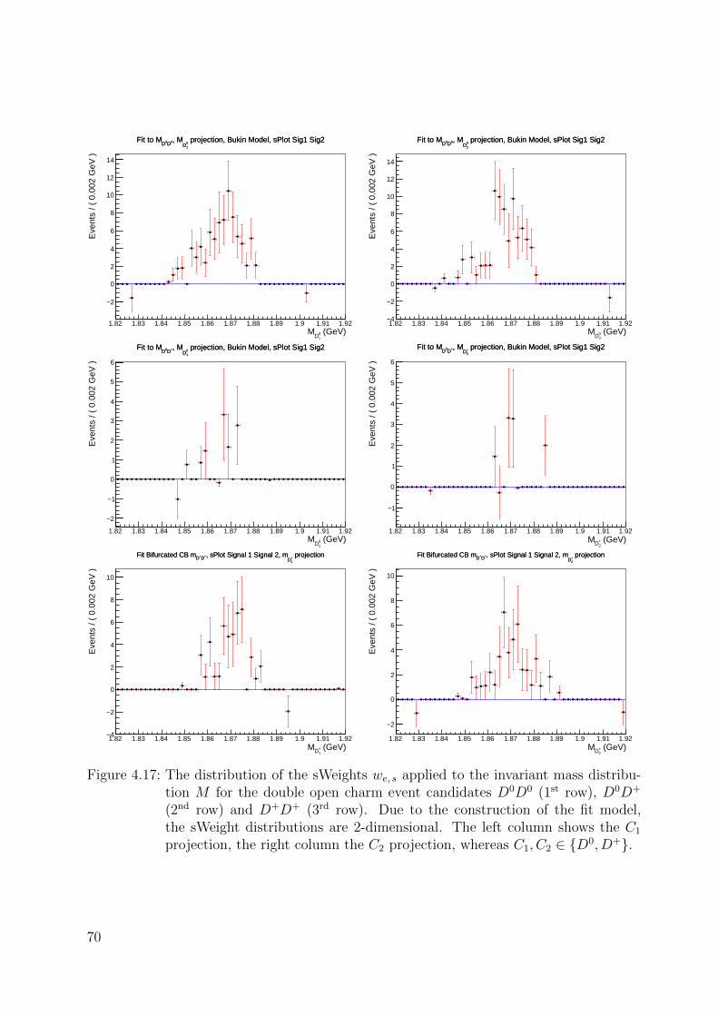
(GeV)10D
M1.82 1.83 1.84 1.85 1.86 1.87 1.88 1.89 1.9 1.91 1.92
Eve
nts
/ ( 0
.002
GeV
)
2−
0
2
4
6
8
10
12
14
projection, Bukin Model, sPlot Sig1 Sig210D
, M0D0DFit to M projection, Bukin Model, sPlot Sig1 Sig2
10D
, M0D0DFit to M
(GeV)20D
M1.82 1.83 1.84 1.85 1.86 1.87 1.88 1.89 1.9 1.91 1.92
Eve
nts
/ ( 0
.002
GeV
)
4−
2−
0
2
4
6
8
10
12
14
projection, Bukin Model, sPlot Sig1 Sig220D
, M0D0DFit to M projection, Bukin Model, sPlot Sig1 Sig2
20D
, M0D0DFit to M
(GeV)10D
M1.82 1.83 1.84 1.85 1.86 1.87 1.88 1.89 1.9 1.91 1.92
Eve
nts
/ ( 0
.002
GeV
)
2−
1−
0
1
2
3
4
5
6
projection, Bukin Model, sPlot Sig1 Sig210D
, M+D0DFit to M projection, Bukin Model, sPlot Sig1 Sig2
10D
, M+D0DFit to M
(GeV)2+DM
1.82 1.83 1.84 1.85 1.86 1.87 1.88 1.89 1.9 1.91 1.92
Eve
nts
/ ( 0
.002
GeV
)
1−
0
1
2
3
4
5
6
projection, Bukin Model, sPlot Sig1 Sig22+D
, M+D0DFit to M projection, Bukin Model, sPlot Sig1 Sig2
2+D
, M+D0DFit to M
(GeV)1+DM
1.82 1.83 1.84 1.85 1.86 1.87 1.88 1.89 1.9 1.91 1.92
Eve
nts
/ ( 0
.002
GeV
)
4−
2−
0
2
4
6
8
10
projection1+D
, sPlot Signal 1 Signal 2, m+D+DFit Bifurcated CB m projection1+D
, sPlot Signal 1 Signal 2, m+D+DFit Bifurcated CB m
(GeV)2+DM
1.82 1.83 1.84 1.85 1.86 1.87 1.88 1.89 1.9 1.91 1.92
Eve
nts
/ ( 0
.002
GeV
)
2−
0
2
4
6
8
10
projection2+D
, sPlot Signal 1 Signal 2, m+D+DFit Bifurcated CB m projection2+D
, sPlot Signal 1 Signal 2, m+D+DFit Bifurcated CB m
Figure 4.17: The distribution of the sWeights we, s applied to the invariant mass distribu-tion M for the double open charm event candidates D0D0 (1st row), D0D+
(2nd row) and D+D+ (3rd row). Due to the construction of the fit model,the sWeight distributions are 2-dimensional. The left column shows the C1
projection, the right column the C2 projection, whereas C1, C2 ∈ {D0, D+}.
70

4.6 Efficiency
The total efficiency for each event candidate e, εtot; e, is a product of four terms:
εtot; e = εacc; e εrec; e ξtrk; e εPID; e εtrg; e ,
where εacc; e : acceptance
εrec; e : reconstruction and selection efficiency
ξtrk; e : tracking efficiency correction factor
εPID; e : particle identification efficiency
εtrg; e : trigger efficiency .
(4.15)
Except for the trigger efficiency εtrg, all other efficiencies, i.e. εacc, εrec (including ξtrk), εPID,are taken from the analysis [28] resp. [29]. Therefore the same event selection as in [28],[29] needs to be applied for this analysis as explained in chapter 4.2.1. The efficiency foran event e is extracted by a two- resp. three-dimensional linear interpolation for that evente. The functional dependence determines the dimensionality of the interpolation. Due tothe pT and y dependence, the two-dimensional interpolation is used for the acceptance, thereconstruction and selection efficiency and the trigger efficiency. Since the PID efficiencydepends on p, η and Ntracks, a three-dimensional linear interpolation is required.
Since a cut on the invariant mass for the single open charm candidates is applied (seechapter 4.2.1, Tab. 4.3), there is in principle a corresponding efficiency to be calculated.The cut 1.82 < MC < 1.92 GeV, C ∈ {D0, D+} is applied, in order to set MD0 and mD+
distributions to the same range for the fits (see chapter 4.4). Initially MD0 had a range of[1.79, 1.94], MD+ a range of about [1.816, 1.924]. Considering the sWeight distributions forthe single open charm event candidates (see Fig. 4.16), the small signal contribution withinthe ranges [1.82, 1.83] and [1.91, 1.92], can be neglected. Since the signal contribution isnot expected to rise below 1.82 GeV and above 1.92 GeV, it can be assumed, that nosignal candidate is lost when applying 1.82 < MC < 1.92 GeV. Therefore the efficiencycorreponding to the mass window can be set to unity.
Acceptance εaccεaccεacc
The acceptance needs to be introduced, since the LHCb detector has a finite spatial ac-ceptance. Only the forward region in the pseudorapidity range 2 < η < 5 is instrumented(equal to a range of the scattering angle θ of about 10 mrad < θ < 250 mrad), so onlyparticles flying inside this region can be detected.
The acceptance is obtained from Monte Carlo simulation using the GAUSS v45r3 frame-work [38], [39]. It is estimated by:
εacc =Nacc
Nprompt
, (4.16)
where Nprompt is the number of generated prompt charm candidates in a (pT , y)-bin andNacc is the number of charm hadrons in that (pT , y)-bin, which pass the generator-level
71

cuts (see [28], [29]). The estimator εacc is a Binomial distributed random variable, whereasthe Binomial PDF is given by:
B(p; k, n) =
(n
k
)pk (1− p)n−k ,
where n : number of trials in a counting experiment
k : number of successes
p ∈ (0, 1) : probability of success .
(4.17)
Consequently the corresponding statistical uncertainty is estimated by:
σεacc =
√εacc(1− εacc)
Nprompt
. (4.18)
The acceptance for the open charm event candidates D0 and D+ is shown in Fig. 4.18.The estimated statistical uncertainties are in general not symmetric, which would lead toasymmetric uncertainties in each (pT , y)-bin in Fig. 4.18. However, they are approximatedsymmetrically, which holds, if the corresponding efficiency in a certain (pT , y)-bin is nottoo small or large.εacc for the double open charm event candidates (including open charm pair production)
can be decomposed into the efficiency of the single open charm event candidates:
εacc; e =
{εacc, C; e single open charm event
εacc, C; e εacc, C; e double open charm event,
where εacc, C; e , C ∈ {D0, D+} : Acceptance for the single open charm
event candidate(s) .
(4.19)
[GeV]0D
Tp2 4 6 8 10 12 14 16 18 20
0Dy
2
2.5
3
3.5
4
4.5
0
0.1
0.2
0.3
0.4
0.5
0.6
0.7
0.8
0.9
1
[GeV]+D
Tp2 4 6 8 10 12 14 16 18 20
+Dy
2
2.5
3
3.5
4
4.5
0
0.1
0.2
0.3
0.4
0.5
0.6
0.7
0.8
0.9
1
Figure 4.18: The acceptance εacc as a function of pT and y for D0 → K−π+ (left) and D+ →K−π+π+ (right) decays, taken from the analysis [28], [29]. The statisticalerrors in each (pT , y)-bin are symetrically approximated.
72

Reconstruction and Selection Efficiency εrecεrecεrec
εrec; e is given by the product of the efficiencies for the event reconstruction and for theapplied event selection without any PID cuts (see chapter 4.2.1). The PID efficiency cor-reponding to the PID selection is determined separately. The reconstruction and selectionefficiency is determined in the same way as the acceptance (see equation 4.17, 4.18). Con-sequently, εrec is determined from Monte-Carlo simulation and is a function of the opencharm candidate’s pT and y. The obtained reconstruction and selection efficieny is cor-rected by the factor ξtrk [40]. This correction factor is determined in an independent studyof a pure Jψ → µ+µ− sample by a tag and probe method. It corrects for the differencesin the track reconstruction between the Monte Carlo simulation and the data sample andis a function of the track momentum ptrk and pseudorapidity ηtrk. The reconstruction andselection efficiency together with the correction factor is shown in Fig. 4.19. The statisti-cal uncertainties in each (pT , y)-bin are symmetrically approximated as for the acceptance.Since ξtrk is limited to p ∈ [5, 201) GeV and η ∈ [1.9, 4.9), the correction factor for can-didates with a (p, η), which exceed those limits, are given the efficiency corresponding top = 5.001 resp. 199.9 GeV and η = 2.001 resp. 4.899.
For the double open charm event candidates (including open charm pair production),εrec can be decomposed into the efficiency of the single open charm event candidates andthe correction factors:
εrec; e =
{εrec, C; e ξtrk; e single open charm event
εrec, C; e ξtrk; e εrec, C; e ξtrk; e double open charm event,
where εrec, C; e, C ∈ {D0D+} : reconstruction and selection efficiency for the
single open charm event candidate(s)
ξtrk; e : correction factor for the single open charm
event candidate(s) .
(4.20)
ξtrk; e for a single open charm event candidate is given by the product of the correctionfactors for each track produced by this open charm event:
ξtrk; e =∏j=trk
ξe, j (pj, ηj) ,
where ξe, j(pj, ηj) : correction factor per track j∏j=trk
: product running over all final state tracks of the
associated single open charm event, i.e. the K− and π+ .
(4.21)
73

[GeV]0D
Tp5 10 15 20
0Dy
2
2.5
3
3.5
4
4.5
0
0.05
0.1
0.15
0.2
0.25
0.3
0.35
0.4
0.45
0.5
[GeV]+DTp
5 10 15 20
+Dy
2
2.5
3
3.5
4
4.5
0
0.05
0.1
0.15
0.2
0.25
0.3
0.35
0.4
0.45
0.5
[GeV]trk
p50 100 150 200
trk
η
2
2.5
3
3.5
4
4.5
0.99
1
1.01
1.02
1.03
1.04
1.05
1.06
1.07
Figure 4.19: The reconstruction and selection efficiency εrec as a function of pT and y forD0 → K−π+ (top left) and D+ → K−π+π+ (top right) decays and for thecorrection factor ξtrk as a function of p and η for the track candidates K− andπ+ (bottom left), taken from the analysis [28], [29]. The statistical errors ineach (pT , y)-bin are symetrically approximated.
74

PID Efficiency εPID; eεPID; eεPID; e
The PID efficiency for the kaon and pion have been determined in [28], [29] from theanalysis of calibration samples of the decay D∗+ →
(D0 → K−π+
)π+ using the PIDCalib
framework [42], [43], [44], [45]. εPID is estimated by:
εPID =Nacc
Nacc +Nrej
=
(1 +
Nrej
Nacc
)−1
, (4.22)
where Nacc is the number of accepted kaon resp. pion candidates in a (p, η,Ntracks)-bin, Nrej
is the number of rejected kaon resp. pion candidates in that (p, η,Ntracks)-bin, according tothe PID selection criteria (see chapter 4.2.1) andNtracks is the number of track multiplicities.Nacc and Nrej are given by sums over per event weights:
Nacc =∑i=acc
wi
Nrej =∑j=rej
wj .(4.23)
These weights wi, wj can be determined using the sP lot method (see chapter 4.5). Due tothis, the estimator εPID is not a Binomial distributed random variable, and the statisticaluncertainty σεPID
needs to be estimated differently than for εacc. The PID efficiency forthe kaon and pionpion final states is illustrated in Fig. 4.20 resp. Fig. 4.21. Similarto the acceptance the statistical uncertainties in each (p, η,Ntracks)-bin are symmetricallyapproximated, since they are in general not symmetric. For certain (p, η,Ntracks)-bins thePID efficiency has values εPID /∈ (0, 1]. For these cases the bin color in Fig. 4.20, 4.21 iswhite. The reason for this is, that for a low number of calibration events, equation 4.22can yield unphysical numbers for the efficiency [29]. The corresponding event candidates,which would fall into such a bin by the interpolation, is assigned a PID efficiency ofεPID; e = 0.5± 0.5. This occurs at the boundaries of the acceptance and is rare.εPID for a single or double open charm event candidate (including open charm pair
production) is given by the product of all identification efficiencies for the K− and π+ finalstate tracks:
εPID; e =∏j=K−
εK−; e, j
∏j=π+
επ+; e, j ,
where εK−; e, j, επ+; e, j : efficiencies for K− and π+ identification∏j=K−
,∏j=π+
: products running over all K− resp. π+ final state tracks of the
associated single or double open charm event (including open
charm pair production) .(4.24)
75

[MeV]K
p20 40 60 80 100 120 140
310×
Kη
2
2.5
3
3.5
4
4.5
0
0.1
0.2
0.3
0.4
0.5
0.6
0.7
0.8
0.9
1
[MeV]K
p20 40 60 80 100 120 140
310×
Kη
2
2.5
3
3.5
4
4.5
0
0.1
0.2
0.3
0.4
0.5
0.6
0.7
0.8
0.9
1
[MeV]K
p20 40 60 80 100 120 140
310×
Kη
2
2.5
3
3.5
4
4.5
0
0.1
0.2
0.3
0.4
0.5
0.6
0.7
0.8
0.9
1
[MeV]K
p20 40 60 80 100 120 140
310×
Kη
2
2.5
3
3.5
4
4.5
0
0.1
0.2
0.3
0.4
0.5
0.6
0.7
0.8
0.9
1
Figure 4.20: The PID efficiency εPID; e as a function of p and η for the kaon candidatesfor four bins in the track multiplicity Ntracks: Ntracks ∈ [0, 150) (top left),Ntracks ∈ [150, 250) (top right), Ntracks ∈ [250, 400) (bottom left) and Ntracks ∈[400, 1000) (bottom right), taken from the analysis [28], [29]. The statisticalerrors in each (p, η,Ntracks)-bin are symetrically approximated.
76

[MeV]πp20 40 60 80 100 120 140
310×
πη
2
2.5
3
3.5
4
4.5
0
0.1
0.2
0.3
0.4
0.5
0.6
0.7
0.8
0.9
1
[MeV]πp20 40 60 80 100 120 140
310×
πη
2
2.5
3
3.5
4
4.5
0
0.1
0.2
0.3
0.4
0.5
0.6
0.7
0.8
0.9
1
[MeV]πp20 40 60 80 100 120 140
310×
πη
2
2.5
3
3.5
4
4.5
0
0.1
0.2
0.3
0.4
0.5
0.6
0.7
0.8
0.9
1
[MeV]πp20 40 60 80 100 120 140
310×
πη
2
2.5
3
3.5
4
4.5
0
0.1
0.2
0.3
0.4
0.5
0.6
0.7
0.8
0.9
1
Figure 4.21: The PID efficiency εPID; e as a function of p and η for the pion candidatesfor four bins in the track multiplicity Ntracks: Ntracks ∈ [0, 150) (top left),Ntracks ∈ [150, 250) (top right), Ntracks ∈ [250, 400) (bottom left) and Ntracks ∈[400, 1000) (bottom right), taken from the analysis [28], [29]. The statisticalerrors in each (p, η,Ntracks)-bin are symetrically approximated.
77

Trigger Efficiency εtrgεtrgεtrg
The trigger efficiency is determined directly on the data sample using the TISTOS method.It exploits the fact, that events with single open charm candidates can be triggered eitherby the selected decay products of the single open charm candidates (TOS: trigger on signal)or by the rest of the event (TIS: trigger independently of signal) [2], [3], [46], [47], [48], [49],[50] [51]. The overlap between these two cases allows the trigger efficiency to be calculated:
εtrg =NTOS∧TIS
NTIS
, (4.25)
where NTOS∧TIS is the number of TIS and TOS events in a (pT , y)-bin, NTIS is the numberof TIS events in that (pT , y)-bin and ∧ is the logical and-operator (logical conjunction).Likewise to the acceptance, the trigger efficiency is estimated as a Binomial distributedrandom variable (see equation 4.17). However, the statistical uncertainties are estimatedby the Clopper-Pearson intervals xl and xu within the 68.3% confidence level [52], recom-mended by the PDG [7]. xl, xu are given by:
1± 0.683
2= Pl(x, a, b) =
1
B(a, b)
∫ x
0
ta−1 (1− t)b−1 dt ,
where B(a, b) =Γ(a)Γ(b)
Γ(a+ b)=
∫ 1
0
ta−1(1− t)b−1 dt
Beta function (Euler’s integral of the first kind)
xl is given by Pl(x, a, b) =1− 0.683
2for a = k, b = n− k + 1
xu is given by Pl(x, a, b) =1 + 0.683
2for a = k + 1, b = n− k
B(p; k, n) = Pl(x; a = k, b = n− k + 1)
Relation between the Binomial PDF and Beta PDF
used for the calculation .
(4.26)
Pl(x, a, b) is the lower tail probability related to the Beta PDF (see chapter 3.1.2, formula3.13 and 3.14). Similar to equation 3.16 the Beta CDF can be splitted into the lower andupper tail probability, i.e. C(β(x; a, b)) = Pl(x, a, b) + Pu(x, a, b), where the Beta PDFB(x; a, b) and its CDF C(B(x; a, b)) are given by:
78

B(x; a, b) =1
B(a, b)xa−1 (1− x)b−1
C(B(x; a, b)) =1
B(a, b)
∫ 1
0
ta−1 (1− t)b−1 dt ,
where x ∈ (0, 1) : observable
a > 0, b > 0 : shape parameters .
(4.27)
Moreover, C(B(x; a, b)) can be expressed in terms of the lower- and upper regularizedincomplete Beta functions βl(x, a, b), βu(x, a, b), such that Pl(x, a, b) and Pu(x, a, b) areforms of βl(x, a, b) and βu(x, a, b).
The TISTOS method requires, that all single open charm event candidates are selectedto be triggered as signal. This is because it determines the efficiency for an event to betriggered on signal, rather than the probability for an event to be triggered at all. Thereforeall those candidates passing the trigger lines listed in Tab. 4.1 (see also chapter 4.2.1) mustfulfill the TOS requirement in addition. In the case of a double open charm or open charmpair production event candidate, one of two choices can be realized. The first is to requireone of the two single open charm candidates to be TOS, the second to require both to beTOS. In order not to loose event candidates unnecessarily, the first choice is picked. Thisleads to the combination formula 4.28. The trigger efficiency for the open charm eventcandidates D0 and D+ is shown in Fig. 4.22.
Similar to the acceptance, εtrg for the double open charm event candidates (includingopen charm pair production) can be decomposed into the efficiency for the single opencharm event candidates:
εtrg; e =
{εtrg, C; e single open charm event
1− (1− εtrg, C; e) (1− εtrg, C; e) double open charm event
where εtrg, C; e , C ∈ {D0, D+} : Trigger efficiency for the single open charm
event candidate(s)
(4.28)
Even though allowing to trigger on any of the D mesons rather than requiring both Dmesons to be TOS increases the trigger efficiency, it also increases the uncertainty on themeasurement of the cross sections. Unfortunately due to the small integrated luminosityonly a small number of events remain for double open charm and pair production candidates(see 4.5).
79
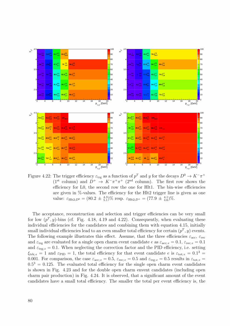
[GeV]0T D
p2 4 6 8 10 12 14 16 18 20
0Dy
2
2.5
3
3.5
4
4.5
0
10
20
30
40
50
60
70
80
90
100
1.2 10.5 39.2 65.9 86.4
1.5 8.9 31.3 56.7 80.7
1.7 9.7 36.3 62.4 86.5
2.9 13.9 47.3 75 90.1
4.3 18.5 53.7 83.3
0.3 0.6 1.3 1.7 1.1
0.1 0.4 0.9 1.5 1.3
0.2 0.4 1.2 1.9 1.5
0.3 0.7 1.7 2.6 2.9
0.6 1.5 4.2 8.9
-0.2 -0.6 -1.2 -1.7 -1.2
-0.1 -0.4 -0.9 -1.5 -1.3
-0.1 -0.4 -1.2 -1.9 -1.7
-0.2 -0.7 -1.7 -2.8 -3.7
-0.5 -1.4 -4.2 -13.6
[GeV]+T Dp
2 4 6 8 10 12 14 16 18 20
+Dy
2
2.5
3
3.5
4
4.5
0
10
20
30
40
50
60
70
80
90
100
0.5 4.3 17.1 42.7 73.1
1.4 4.2 15.8 34.5 68.9
1.5 5 17.3 43.2 74.3
2.6 7.2 27.6 58.7 80.1
3.1 9.8 43.2 79.3
0.5 0.5 1.1 1.8 1.4
0.2 0.3 0.7 1.3 1.3
0.2 0.3 0.9 1.7 1.7
0.3 0.5 1.5 2.6 3.1
1 1.4 4.2 7.9
-0.3 -0.5 -1 -1.8 -1.5
-0.2 -0.3 -0.7 -1.3 -1.4
-0.2 -0.3 -0.8 -1.7 -1.8
-0.3 -0.5 -1.4 -2.7 -3.5
-0.8 -1.3 -4.1 -10.3
[GeV]0T D
p2 4 6 8 10 12 14 16 18 20
0Dy
2
2.5
3
3.5
4
4.5
0
10
20
30
40
50
60
70
80
90
100
63.3 76.7 80.8 86.1 82.5
71.7 79.6 81.3 86.7 93.1
72.5 80.8 82.9 89.2 89.9
74.6 81.9 92.1 95.4 97.7
72.6 91.3 93.8 100
7.5 3 2 2.1 2.2
3.8 1.9 1.7 1.9 1.4
3.6 2.1 1.8 1.9 2.1
3.3 1.9 1.6 1.8 1.9
4.8 2.3 2.9
-8.1 -3.2 -2.1 -2.4 -2.4
-4.1 -2.1 -1.9 -2.1 -1.6
-3.8 -2.2 -2 -2.2 -2.5
-3.6 -2 -1.9 -2.6 -5.1
-5.3 -2.8 -4.6 -45.9
[GeV]+T Dp
2 4 6 8 10 12 14 16 18 20
+Dy
2
2.5
3
3.5
4
4.5
0
10
20
30
40
50
60
70
80
90
100
80 81.1 85 84.8 90.8
57.1 91.7 91.4 92.6 93.8
67.1 86.4 90.4 94.4 94.5
64 86.6 94.3 96.6 100
65.4 85.5 95.5 100
12.8 4.7 3 2.7 1.7
6.8 2.1 1.7 1.6 1.3
5.9 2.4 1.8 1.6 1.5
5.4 2.5 1.7 1.6
10.3 4.1 2.9
-20.5 -5.7 -3.5 -3.2 -2
-7.1 -2.7 -2.1 -2 -1.6
-6.4 -2.8 -2.1 -2.1 -2
-5.8 -2.9 -2.2 -2.6 -3.4
-11.7 -5.2 -5.7 -10.3
Figure 4.22: The trigger efficiency εtrg as a function of pT and y for the decays D0 → K−π+
(1st column) and D+ → K−π+π+ (2nd column). The first row shows theefficiency for L0, the second row the one for Hlt1. The bin-wise efficienciesare given in %-values. The efficiency for the Hlt2 trigger line is given as onevalue: εHlt2;D0 = (80.2 ± 4.3
5.1)% resp. εHlt2;D+ = (77.9 ± 4.14.6)%.
The acceptance, reconstruction and selection and trigger efficiencies can be very smallfor low (pT , y)-bins (cf. Fig. 4.18, 4.19 and 4.22). Consequently, when evaluating theseindividual efficiencies for the candidates and combining them with equation 4.15, initiallysmall individual efficiencies lead to an even smaller total efficiency for certain (pT , y) events.The following example illustrates this effect. Assume, that the three efficiencies εacc, εrec
and εtrg are evaluated for a single open charm event candidate e as εacc; e = 0.1, εrec; e = 0.1and εtrg; e = 0.1. When neglecting the correction factor and the PID efficiency, i.e. settingξtrk; e = 1 and εPID = 1, the total efficiency for that event candidate e is εtot; e = 0.13 =0.001. For comparison, the case εacc; e = 0.5, εrec; e = 0.5 and εtrg; e = 0.5 results in εtot; e =0.53 = 0.125. The evaluated total efficiency for the single open charm event candidatesis shown in Fig. 4.23 and for the double open charm envent candidates (including opencharm pair production) in Fig. 4.24. It is observed, that a significant amount of the eventcandidates have a small total efficiency. The smaller the total per event efficiency is, the
80
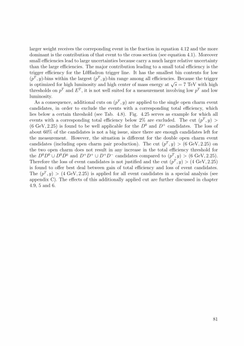
larger weight receives the correponding event in the fraction in equation 4.12 and the moredominant is the contribution of that event to the cross section (see equation 4.1). Moreoversmall efficiencies lead to large uncertainties because carry a much larger relative uncertaintythan the large efficiencies. The major contribution leading to a small total efficiency is thetrigger efficiency for the L0Hadron trigger line. It has the smallest bin contents for low(pT , y)-bins within the largest (pT , y)-bin range among all efficiencies. Because the triggeris optimized for high luminosity and high center of mass energy at
√s = 7 TeV with high
thresholds on pT and ET , it is not well suited for a measurement involving low pT and lowluminosity.
As a consequence, additional cuts on (pT , y) are applied to the single open charm eventcandidates, in order to exclude the events with a corresponding total efficiency, whichlies below a certain threshold (see Tab. 4.8). Fig. 4.25 serves as example for which allevents with a corresponding total efficiency below 2% are excluded. The cut (pT , y) >(6 GeV, 2.25) is found to be well applicable for the D0 and D+ candidates. The loss ofabout 60% of the candidates is not a big issue, since there are enough candidates left forthe measurement. However, the situation is different for the double open charm eventcandidates (including open charm pair production). The cut (pT , y) > (6 GeV, 2.25) onthe two open charm does not result in any increase in the total efficiency threshold forthe D0D0 ∪ D0D0 and D+D+ ∪ D+D− candidates compared to (pT , y) > (6 GeV, 2.25).Therefore the loss of event candidates is not justified and the cut (pT , y) > (4 GeV, 2.25)is found to offer best deal between gain of total efficiency and loss of event candidates.The (pT , y) > (4 GeV, 2.25) is applied for all event candidates in a special analysis (seeappendix C). The effects of this additionally applied cut are further discussed in chapter4.9, 5 and 6.
81

Candidate Cut on (pT [GeV], y) εtot, thres [%] fcut =Ntot, cut
Ntot, init[%]
D0 (2, 2) 0.02 100
(4, 2.25) 0.29 85.1
(6, 2.25) 1.89 54.9
D+ (2, 2) 0.01 100
(4, 2.25) 0.08 90.7
(6, 2.25) 0.61 68.4
D0D0 ∪D0D0 (2, 2) 0.02 100
(4, 2.25) 0.02 72.4
(6, 2.25) 0.02 56.3
D0D+ ∪D0D− (2, 2) 0.03 100
(4, 2.25) 0.03 100
(6, 2.25) 0.15 72.7
D+D+ ∪D+D+ (2, 2) 0.003 100
(4, 2.25) 0.06 84.3
(6, 2.25) 0.06 80.4
Table 4.8: Additional applied cuts on (pT , y) for the single open charm event candidatesD0, D+ and double open charm event candidates (including open charm pairproduction) {D0D0 ∪ D0D0} ,{D0D+ ∪ D0D−} and {D+D+ ∪ D+D−}. Thecorresponding total efficiencies of all selected events is above εtot, thres [%]. Com-pared to the initial cut of (pT , y) > (2 GeV, 2), the fraction fcut [%] remain inthe dataset. (see 4.3).
82

[GeV]0D
Tp2 4 6 8 10 12 14 16 18 20
0Dy
2
2.5
3
3.5
4
4.5
0
0.02
0.04
0.06
0.08
0.1
0.12
0.14
0tot; Dε
0 0.02 0.04 0.06 0.08 0.1 0.12 0.14
Eve
nts
/ 0.0
025
0
1000
2000
3000
4000
5000
[GeV]+D
Tp2 4 6 8 10 12 14 16 18 20
+Dy
2
2.5
3
3.5
4
4.5
0
0.02
0.04
0.06
0.08
0.1
0.12
0.14
+tot; Dε0 0.02 0.04 0.06 0.08 0.1 0.12 0.14
Eve
nts
/ 0.0
025
0
500
1000
1500
2000
2500
3000
3500
4000
Figure 4.23: The bin-wise averaged evaluated total efficiency εtot; e as a function of pT andy for the single open charm event candidates D0 (1st row) and D+ (2nd row).
83

[GeV]0D0D
Tp0 5 10 15 20 25
0D
0Dy
2
2.5
3
3.5
4
4.5
0
0.005
0.01
0.015
0.02
0.025
0.03
0.035
0D0tot; Dε
0 0.005 0.01 0.015 0.02 0.025 0.03 0.035
Eve
nts
/ 0.0
01
0
2
4
6
8
10
[GeV]+D0D
Tp0 5 10 15 20 25
+D
0Dy
2
2.5
3
3.5
4
4.5
0
0.005
0.01
0.015
0.02
0.025
0.03
0.035
+D0tot; Dε
0 0.005 0.01 0.015 0.02 0.025 0.03 0.035
Eve
nts
/ 0.0
01
0
0.2
0.4
0.6
0.8
1
1.2
1.4
1.6
1.8
2
[GeV]+D+D
Tp0 5 10 15 20 25
+D
+Dy
2
2.5
3
3.5
4
4.5
0
0.005
0.01
0.015
0.02
0.025
0.03
0.035
+D+tot; Dε0 0.005 0.01 0.015 0.02 0.025 0.03 0.035
Eve
nts
/ 0.0
01
0
1
2
3
4
5
6
7
Figure 4.24: The bin-wise averaged evaluated total efficiency εtot; e as a function of pT andy for the double open charm event candidates D0D+ (1st row), D0D+ (2nd
row) and D+D+ (3rd row).
84

[GeV]0T D
p2 4 6 8 10 12 14 16 18 20
0Dy
2
2.5
3
3.5
4
4.5
0
0.02
0.04
0.06
0.08
0.1
0.12
0.14
[GeV]+D
Tp2 4 6 8 10 12 14 16 18 20
+Dy
2
2.5
3
3.5
4
4.5
0
0.02
0.04
0.06
0.08
0.1
0.12
0.14
[GeV]0D0D
Tp0 5 10 15 20 25
0D
0Dy
2
2.5
3
3.5
4
4.5
0
0.005
0.01
0.015
0.02
0.025
0.03
0.035
[GeV]+D0D
Tp0 5 10 15 20 25
+D
0Dy
2
2.5
3
3.5
4
4.5
0
0.005
0.01
0.015
0.02
0.025
0.03
0.035
[GeV]+D+D
Tp0 5 10 15 20 25
+D
+Dy
2
2.5
3
3.5
4
4.5
0
0.005
0.01
0.015
0.02
0.025
0.03
0.035
Figure 4.25: The bin-wise averaged evaluated total efficiency εtot; e as a function of pT andy of the single open charm and combined double open charm (or open charmpair production) system for the D0 (top left), D+ (top right), D0D0 ∪D0D0
(center left), D0D+∪D0D− (center right) and D+D+∪D+D− (bottom right)event candidates for an efficiency threshold of εtot, thres; e > 2%.
85

4.6.1 Global Event Cut Efficiency
The global event selection is applied on the trigger level in order to reject events with a largenumber of hits in the detector. For the trigger lines L0Hadron Dec and Hlt1TrackAllL0 Dec,a cut is applied on the number of SPD hits, NSPD < 600. SPD is the abbreviation for thescintillating pad detector in the calorimetry system of the LHCb detector (see ch. 3.1.1).Initially the global event selection consisted of two cuts, NSPD < 600 and NOT < 10000. Inthe whole data sample there is only one event that passes the event selection but not therequirement on NOT. This event passes the trigger on another trigger line. Therefore itseffect on the NOT distribution is neglected and the global event cut (GEC) efficiency εGEC,can be calculated without taking NOT into account. Consequently, the GEC efficiency,εGEC, can be calculated solely from an unbinned maximum likelihod fit to the distributionof NSPD, the SPD hit multiplicities. For the single open charm event candidates, a DoubleGamma PDF, G, is chosen to model the distribution. This PDF is described by:
G(x;µ1, µ2, γ1, γ2, β1, β2) = n1 g1(x;µ1, γ1, β1) + n2 g2(x;µ2, γ2, β2) ,
where gi(x;µi, γi, βi) =
niβi Γ(γi)
(x−µiβi
)γi−1
e−x−µi
βi , x− µi > 0
0 , x− µi < 0, i ∈ {1, 2}
Single Gamma PDF components
Γ(ki) =
∫ ∞0
tki−1 e−t dt Gamma function (Euler’s integral form)
x : observable, i.e. NSPD for the single and double charm event candidates
ki > 0, θi > 0, µi : free parameters of the PDF
ni : normalization factors .(4.29)
For the double open charm event candidates and open charm pair produced event candi-dates a simpler Single Gamma PDF is chosen to model the NSPD distribution. In the sameway as in chapter 4.4 the double open charm and open charm pair production samples aremerged, i.e. CC ∈ {D0D0, D0D+, D+D+} ∪ {D0D0, D0D−, D+D−} to increase the totalnumber of events in the corresponding NSPD distributions. The result of the fit is shownfor the D0 and D+ candidates in Fig. 4.26 and for the D0D0, D0D+, D+D+ including theD0D0, D0D−, D+D− candidates in Fig. 4.27, the corresponding fit parameters in Tab.B.1 and Tab. B.2.
As alternative fit models for the single open charm event candidates, the simpler SingleGamma PDF and stretched Beta PDF have been tested (see equation B.1). However theypion describe the tail of the NSPD distribution as well as the Double Gamma PDF G (cf.Fig. 4.26, 4.28, 4.29 and corresponding fit parameters in Tab. B.1, B.3, B.4). However,the Single Gamma PDF is able to model the NSPD distribution for the double open charmevent candidates due to the lower statistics.
In the actual fitting algorithm the factors ni, 1/βi, 1/Γ(γi) are absorbed into the overall
86

normalization Ni, i.e. Ni = niβi Γ(γi)
, i ∈ {1, 2}. These overall normalization factors donot represent the number of events anymore. To have access to normalization factorsrepresenting number of events, an integral representation can be used. The number ofevents in a given interval [a, b], N[a, b] are given by:
N[a, b] =
∫ b
a
G(x;µ1, µ2, γ1, γ2, β1, β2) dx , a > 0, b > 0, b > a ,
where G(x;µ1, µ2, γ1, γ2, β1, β2) : Double Gamma PDF
x : observable, i.e. NSPD for the cases of the single and double
open charm event candidates .
(4.30)
The GEC efficiency εGEC can then be determined from N[ncutoff,∞], where ncutoff = 600, andN[0,∞] by:
εGEC =N[0, ncutoff]
N[0,∞]
=
∫ ncutoff
0G(x;µ1, µ2, γ1, γ2, β1, β2) dx∫∞
0G(x;µ1, µ2, γ1, γ2, β1, β2) dx
= 1−N[ncutoff,∞]
N[0,∞]
= 1−∫∞ncutoff
G(x;µ1, µ2, γ1, γ2, β1, β2) dx∫∞0G(x;µ1, µ2, γ1, γ2, β1, β2) dx
.
(4.31)
Due to the cut NSPD < 600, the fit model needs to be extrapolated into the regionNSPD ≥ 600, in order to determine the number of events in that region, N[ncutoff,∞]. Forthe calculation of the total number of events, N[0,∞], it is not possible to implement theinfinity, ∞, numerically. Instead, the representation ∞ := 100000 is used. This numberis much larger than the number of cells in the SPD detector, i.e. the maximal value forNSPD. Using uncorrelated systematical error propagation, the uncertainty on εGEC, σεGEC
,is given by:
σεGEC = σN[ncutoff,∞]
1
N[0,∞]
+ σN[0,∞]
N[ncutoff,∞]
N2[0,∞]
(4.32)
The GEC efficiencies for each single and double open charm event candidate (includingopen charm pair production) are listed in Tab. 4.9. It is observed, that the GEC efficiencyis εGEC > 0.9999 in all cases. Therefore the effect on the cross section is very small,such that it can be neglected, i.e. εGEC can be set to unity. This is a much larger GECefficiency than it is usually observed in high luminosity data taking. This is due to thereduced number of visible interactions (µ ' 1) in the used data taking period for thismeasurement.
87
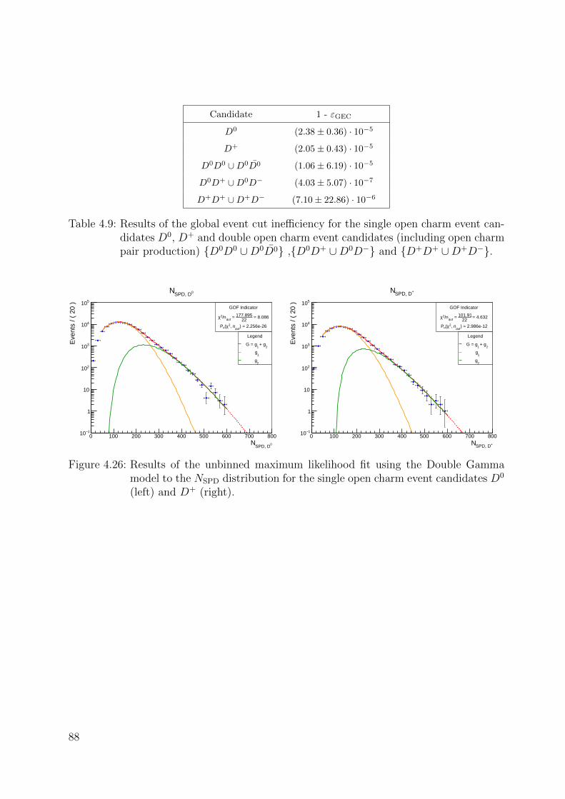
Candidate 1 - εGEC
D0 (2.38± 0.36) · 10−5
D+ (2.05± 0.43) · 10−5
D0D0 ∪D0D0 (1.06± 6.19) · 10−5
D0D+ ∪D0D− (4.03± 5.07) · 10−7
D+D+ ∪D+D− (7.10± 22.86) · 10−6
Table 4.9: Results of the global event cut inefficiency for the single open charm event can-didates D0, D+ and double open charm event candidates (including open charmpair production) {D0D0 ∪D0D0} ,{D0D+ ∪D0D−} and {D+D+ ∪D+D−}.
0SPD, DN
0 100 200 300 400 500 600 700 800
Eve
nts
/ ( 2
0 )
1−10
1
10
210
310
410
510GOF Indicator
= 8.08622
177.895 = dof
/n2χ
) = 2.256e-26dof
, n2χ(uP
Legend
2 + g
1G = g
1g
2g
0SPD, DN
+SPD, DN0 100 200 300 400 500 600 700 800
Eve
nts
/ ( 2
0 )
1−10
1
10
210
310
410
510GOF Indicator
= 4.63222
101.91 = dof
/n2χ
) = 2.986e-12dof
, n2χ(uP
Legend
2 + g
1G = g
1g
2g
+SPD, DN
Figure 4.26: Results of the unbinned maximum likelihood fit using the Double Gammamodel to the NSPD distribution for the single open charm event candidates D0
(left) and D+ (right).
88

0D0SPD, DN
0 100 200 300 400 500 600 700 800
Eve
nts
/ ( 4
0 )
5−10
4−10
3−10
2−10
1−10
1
10
210
310GOF Indicator
= 0.46711
5.136 = dof
/n2χ
) = 0.924dof
, n2χ(uP
0D0SPD, DN
+D0SPD, DN
0 100 200 300 400 500 600 700 800
Eve
nts
/ ( 4
0 )
5−10
4−10
3−10
2−10
1−10
1
10
210GOF Indicator
= 0.41411
4.555 = dof
/n2χ
) = 0.951dof
, n2χ(uP
Legend
1G = g
+D0SPD, DN
+D+SPD, DN0 100 200 300 400 500 600 700 800
Eve
nts
/ ( 4
0 )
5−10
4−10
3−10
2−10
1−10
1
10
210
310GOF Indicator
= 0.52111
5.73 = dof
/n2χ
) = 0.891dof
, n2χ(uP
Legend
1G = g
+D+SPD, DN
Figure 4.27: Results of the unbinned maximum likelihood fit using the double Gammamodel to the NSPD distribution for the double open charm event candidates(including open charm pair production) {D0D0 ∪D0D0} (top left), {D0D+ ∪D0D−} (top right), {D+D+ ∪D+D−} (bottom left).
89
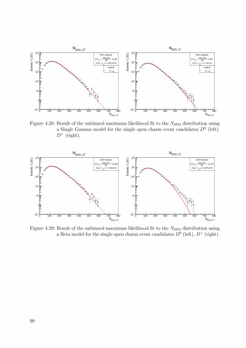
0SPD, DN
0 100 200 300 400 500 600 700 800
Eve
nts
/ ( 2
0 )
1−10
1
10
210
310
410
510GOF Indicator
= 11.8826
308.892 = dof/n2χ
) = 3.507e-50dof
, n2χ(uP
Legend
1G = g
0SPD, DN
+SPD, DN0 100 200 300 400 500 600 700 800
Eve
nts
/ ( 2
0 )
1−10
1
10
210
310
410
510GOF Indicator
= 5.99726
155.909 = dof/n2χ
) = 1.73e-20dof
, n2χ(uP
Legend
1G = g
+SPD, DN
Figure 4.28: Result of the unbinned maximum likelihood fit to the NSPD distribution usinga Single Gamma model for the single open charm event candidates D0 (left),D+ (right).
0SPD, DN
0 100 200 300 400 500 600 700 800
Eve
nts
/ ( 2
0 )
1−10
1
10
210
310
410
510GOF Indicator
= 12.54526
326.178 = dof/n2χ
) = 1.184e-53dof
, n2χ(uP
0SPD, DN
+SPD, DN0 100 200 300 400 500 600 700 800
Eve
nts
/ ( 2
0 )
1−10
1
10
210
310
410
510GOF Indicator
= 12.78726
332.472 = dof/n2χ
) = 6.387e-55dof
, n2χ(uP
+SPD, DN
Figure 4.29: Result of the unbinned maximum likelihood fit to the NSPD distribution usinga Beta model for the single open charm event candidates D0 (left), D+ (right).
90
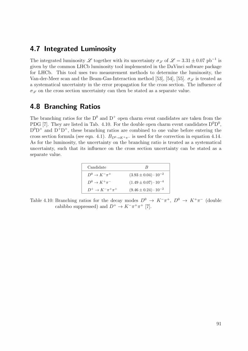
4.7 Integrated Luminosity
The integrated luminosity L together with its uncertainty σL of L = 3.31± 0.07 pb−1 isgiven by the common LHCb luminosity tool implemented in the DaVinci software packagefor LHCb. This tool uses two measurement methods to determine the luminosity, theVan-der-Meer scan and the Beam-Gas-Interaction method [53], [54], [55]. σL is treated asa systematical uncertainty in the error propagation for the cross section. The influence ofσL on the cross section uncertainty can then be stated as a separate value.
4.8 Branching Ratios
The branching ratios for the D0 and D+ open charm event candidates are taken from thePDG [7]. They are listed in Tab. 4.10. For the double open charm event candidates D0D0,D0D+ and D+D+, these branching ratios are combined to one value before entering thecross section formula (see eqn. 4.1). BD0→K+π− is used for the correction in equation 4.14.As for the luminosity, the uncertainty on the branching ratio is treated as a systematicaluncertainty, such that its influence on the cross section uncertainty can be stated as aseparate value.
Candidate B
D0 → K−π+ (3.93± 0.04) · 10−2
D0 → K+π− (1.49± 0.07) · 10−4
D+ → K−π+π+ (9.46± 0.24) · 10−2
Table 4.10: Branching ratios for the decay modes D0 → K−π+, D0 → K+π− (doublecabibbo suppressed) and D+ → K−π+π+ [7].
91

4.9 Systematic Uncertainties
The major source of systematic uncertainty originates from the determination of the effi-ciencies defined by equation 4.15. Any other source is not considered in this analysis. Thesystematic uncertainty is estimated by a toy Monte Carlo method. First, the efficienciesεacc, εrec, εPID, provided by the analysis [28] resp. [29], and εtrg are randomly varied withintheir uncertainties. ξtrk is not varied, since the corrections are small. For each bin i in thehistograms, its bin content εi is substituted by εi → ε′i. For εacc, εrec, εPID the variation ε′i isgiven by a Gaussian distributed random value truncated to the interval (0, 1], while for εtrg
the variation is given by a Beta distributed random value. The bin contents εi representthe means µi and the symmetrically approximated bin errors σi the standard deviationsσgaus; i of the Gaussian PDF needed to generate the corresponding random values in eachbin i. The Gaussian PDF is given by:
N(x;µ, σ) =1√
2π σexp
(−1
2
(x− µσ
)2)
,
where x : Observable
µ : Mean; also being the expectation value
σ : Standard deviation
(4.33)
For the trigger efficiency the number of events being TOS and TIS, NTOS∧TIS, and thenumber of events being TIS, NTIS, can be identified as the k and n parameters of the Bino-mial distribution, repectively (see equation 4.17). Since the Beta distribution is interpretedas the continuous generalization of the Binomial distribution for real k and n within theinterval (0, 1), the parametrization a = k+1, b = n−k+1 is used determine the two shapeparameters a and b of the Beta PDF needed to generate the corresponding random valuein each bin i (see equation 4.27, 4.26). The case of an unphysical efficiency, i.e. for certainbins of εPID, resulting a uniform PDF within (0, 1), is included in this representation.
Then, all steps to evaluate the the total efficiency for each event candidate e, εtot; e, areexecuted for each variation ε′i. This leads to variations for the total efficiency ε′tot; e, j foreach event candidate e and for each variation j. Using equation 4.1, the procedure leadsto variations for the cross section, σ′j. The cross section distributions obtained from thesetoy experiments are shown in Fig. 4.31 for the single open charm event candidates and inFig. 4.32 and 4.33 for the double open charm event candidates (including open charm pairproduction). It is observed, that these distributions have an upper tail. This behavior islikely caused by those events, which have the smallest total efficiency.
Since the trigger efficiency is observed to be the major cause for small event-wise totalefficiencies (see chapter 4.6), the choice of the Beta PDF is important. It is expected, thatwhen using the Gaussian PDF for the variation of the trigger efficiency instead of the BetaPDF, the cross section distribution obtained from the toy experiments have an even largerupper tail.
92
The tendency for large tails is the reason, that the standard deviation of the variationsis not a viable estimator for the systematical uncertainty on the cross section σana;σ:
σana;σ =
√√√√ 1
nj − 1
nj∑j=1
(σ′j − µ(σ′j)
)2
where µ(σ′j) =1
nj
nj∑j=1
σ′j Mean of the variations σ′j
nj∑j=1
: Sum running over all variations σ′j
(4.34)
Large variated cross section values have a bigger contribution in this equation than smallones, resulting in an overestimation of the systematic uncertainty εana;σ. Therefore, thissystematic uncertainty is determined differently by using the cross section distributionfor the toy experiments. The confidence interval is calculated as the smallest interval,containing 68.3% of the toy experiments. In case nj · 0.683 does not yield an integer, itis set to the next larger integer. The lower- and upper interval boundaries, denoted asLowerBound and UpperBound, are then given by the center value between the variatedcross section value lying inside the interval and the next variated cross section value lyingoutside the interval (see Fig. 4.30). Then, the lower- resp. upper systematic uncertaintiesare estimated as:
σana, low;σ = Mode− LowerBoundσana, high;σ = UpperBound−Mode .
(4.35)
The Mode is calculated analogously to Lower Bound and Upper Bound as the centerbetween the the interval boundaries corresponding to the confidence interval of 0.1. It isdrawn as a red star, while the systematic uncertainty estimations are drawn as black errorbars in Fig. 4.31 to 4.33. This estimate for the systematic uncertainty is referred to as thesystematic uncertainty related to the analysis in chapter 5. For comparison, the unvariedcross section values, the mean, the median and the standard deviation are denoted asBest Value, Mean, Median and RMS. The latter three quantities are calculated based onthe binned cross section distributions. The Best Value is drawn as a green star in Fig.4.31 to 4.33. A substantial number of toy experiments are required, such that statisticalfluctuations can balance out. The number of variations nj = 1000 leads to reasonablepopulated histograms, expecially needed in order to determine the Mode properly.
Bias of the MethodFor some candidates, the cross section values obtained from the toy experiments tend tobe smaller than the Best Value. Sometimes the Best Value is higher than the Lower Bound(see Fig. 4.31). This is expected, since the way the efficencies are varied, lead to efficiencyvalues with a slight bias towards high efficiencies, i.e. low cross sections. This arises fromtruncating the Gaussian PDF to (0, 1] or using the asymmetric Beta PDF for efficiencies
93

less than 0.5. The first hypothesis during the analysis was, that the usage of the truncatedGaussian PDF yielding a finite probability density for efficiencies close to zero leads to theexcessive event weights. This was the reason for replacing the truncated Gaussian PDFwith a Beta PDF for the smallest efficiencies, i.e. the trigger efficiencies. This solves theproblem in a large part, since the bias in the total efficiency and in every event is small,as it can be seen in Fig. 4.34. The current interpretation of this behavior is, that theCentral Limit Theorem holds for sums but not for products like the total efficiency (seeequation 4.15). This explains why the RMS is an inferior estimator for the confidenceinterval. Since the bias is small, the method to propagate the systematic uncertaintieson the efficiencies to the cross section is useful. However, the distributions of the crosssections get more biased the smaller the involved efficiencies are. As expected, the methodworks better for the cross section ratios.
kσ0 0.5 1 1.5 2 2.5 3
0
0.2
0.4
0.6
0.8
1
1.2
1.4
1.6
1.8
2
Figure 4.30: Illustration of the procedure used to estimate the systematic uncertainty onthe cross section σana. In this example of a toy experiment 15 cross sectionvalues are calculated, where k ≤ 15.
94

b]µ [0Dσ
40 45 50 55 60 65 70
/ B
injn
0
10
20
30
40
50
60
70
80
Stat. Values
bµMean = 50.53
bµRMS = 3.12
bµMode = 49.01
bµMedian = 50.50
bµBest Value = 49.82
bµLower Bound = 46.70
bµUpper Bound = 52.73
b]µ [+Dσ10 20 30 40 50 60 70
/ B
injn
0
20
40
60
80
100
120
140
160
180
Stat. Values
bµMean = 17.74
bµRMS = 3.42
bµMode = 16.82
bµMedian = 16.90
bµBest Value = 16.69
bµLower Bound = 15.54
bµUpper Bound = 18.14
Figure 4.31: Cross section distributions obtained from the toy experiments for the singleopen charm event candidates D0 (left) and D+ (right). The mode of a distri-butions is denoted as Mode and drawn as a red star, while the cross sectionvalue calculated by the analysis is denoted as Best V alue and drawn as greentriangle. The parameters LowerBound and UpperBound correspond to thelower and upper end points of the error bar, drawn in pink. The other statis-tics parameter calculated from the binned distributions are the mean, medianand standard deviation, denoted as Mean, Median and RMS.
95

b]µ [0D0Dσ
0.15 0.2 0.25 0.3 0.35 0.4
/ B
injn
0
10
20
30
40
50
60
70
80
Stat. Values
bµMean = 0.25
bµRMS = 0.03
bµMode = 0.24
bµMedian = 0.25
bµBest Value = 0.26
bµLower Bound = 0.22
bµUpper Bound = 0.27
b]µ [0D0Dσ
4 5 6 7 8 9 10 11 12 13 14
/ B
injn
0
20
40
60
80
100
Stat. Values
bµMean = 6.48
bµRMS = 0.53
bµMode = 6.21
bµMedian = 6.45
bµBest Value = 6.35
bµLower Bound = 5.97
bµUpper Bound = 6.77
b]µ [+D0Dσ
0.2 0.25 0.3 0.35 0.4 0.45 0.5
/ B
injn
0
20
40
60
80
100
Stat. Values
bµMean = 0.30
bµRMS = 0.03
bµMode = 0.29
bµMedian = 0.31
bµBest Value = 0.40
bµLower Bound = 0.27
bµUpper Bound = 0.32
b]µ [+D+Dσ0.2 0.4 0.6 0.8 1 1.2 1.4
/ B
injn
0
20
40
60
80
100
120
Stat. Values
bµMean = 0.51
bµRMS = 0.10
bµMode = 0.45
bµMedian = 0.51
bµBest Value = 1.16
bµLower Bound = 0.38
bµUpper Bound = 0.57
b]µ [-D+Dσ0.5 0.55 0.6 0.65 0.7 0.75 0.8 0.85 0.9 0.95 1
/ B
injn
0
10
20
30
40
50
60
70
80
Stat. Values
bµMean = 0.75
bµRMS = 0.05
bµMode = 0.74
bµMedian = 0.74
bµBest Value = 0.74
bµLower Bound = 0.69
bµUpper Bound = 0.79
Figure 4.32: Cross section distributions obtained from the toy experiments for the doubleopen charm event candidates D0D0 (top left), D0D+ (center left), D+D+
(bottom left) and for the open charm pair production event candidates D0D0
(top right) and D+D− (bottom right). No event candidate is observed forthe D0D−. The mode of a distributions is denoted as Mode and drawn as ared star, while the cross section value calculated by the analysis is denotedas Best V alue and drawn as green triangle. The parameters LowerBoundand UpperBound correspond to the lower and upper end points of the errorbar, drawn in pink. The other statistics parameter calculated from the binneddistributions are the mean, median and standard deviation, denoted as Mean,Median and RMS.
96

b]µ [0D0DR6000 7000 8000 9000 10000 11000 12000 13000 14000
/ B
injn
0
10
20
30
40
50
60
70
80
Stat. Values
bµMean = 10151.75
bµRMS = 1057.90
bµMode = 9943.25
bµMedian = 10080.00
bµBest Value = 9504.44
bµLower Bound = 9041.51
bµUpper Bound = 11178.85
b]µ [0D0DR
0 100 200 300 400 500 600
/ B
injn
0
10
20
30
40
50
60
70
80
90
Stat. Values
bµMean = 394.81
bµRMS = 31.69
bµMode = 393.69
bµMedian = 393.00
bµBest Value = 390.61
bµLower Bound = 369.74
bµUpper Bound = 420.46
b]µ [+D0DR2000 2500 3000 3500 4000 4500 5000 5500 6000 6500 7000
/ B
injn
0
10
20
30
40
50
60
70
80
90
Stat. Values
bµMean = 2937.37
bµRMS = 419.60
bµMode = 2878.46
bµMedian = 2875.00
bµBest Value = 2073.02
bµLower Bound = 2568.16
bµUpper Bound = 3078.67
b]µ [+D+DR0 500 1000 1500 2000 2500 3000
/ B
injn
0
20
40
60
80
100
Stat. Values
bµMean = 628.65
bµRMS = 201.60
bµMode = 615.22
bµMedian = 615.00
bµBest Value = 239.68
bµLower Bound = 475.36
bµUpper Bound = 707.28
b]µ [-D+DR200 400 600 800 1000 1200 1400 1600 1800 2000
/ B
injn
0
20
40
60
80
100
120
140
160
180
Stat. Values
bµMean = 421.24
bµRMS = 140.09
bµMode = 366.65
bµMedian = 389.00
bµBest Value = 377.36
bµLower Bound = 339.75
bµUpper Bound = 423.80
Figure 4.33: Cross section ratio (i.e. RCC) distributions obtained from the toy experimentsfor the double open charm event candidates D0D0 (top left), D0D+ (centerleft), D+D+ (bottom left) and for the open charm pair production event can-didates D0D0 (top right) and D+D− (bottom right). No event candidate isobserved for the D0D−. The mode of a distributions is denoted as Mode anddrawn as a red star, while the cross section value calculated by the analy-sis is denoted as Best V alue and drawn as green triangle. The parametersLowerBound and UpperBound correspond to the lower and upper end pointsof the error bar, drawn in pink. The other statistics parameter calculatedfrom the binned distributions are the mean, median and standard deviation,denoted as Mean, Median and RMS.
97

0tot; Dε
0.08 0.09 0.1 0.11 0.12 0.13 0.14 0.15 0.16 0.17 0.18
/ B
injn
0
20
40
60
80
100
0tot; Dε
0 0.1 0.2 0.3 0.4 0.5 0.6 0.7
3−10×
/ B
injn
0
20
40
60
80
100
120
140
+tot; Dε0.08 0.09 0.1 0.11 0.12 0.13 0.14 0.15 0.16 0.17 0.18
/ B
injn
0
20
40
60
80
100
+tot; Dε0 0.1 0.2 0.3 0.4 0.5 0.6 0.7
3−10×
/ B
injn
0
20
40
60
80
100
Figure 4.34: Total efficiency distributions obtained from the toy experiments for the cor-responding largest (1st column) and smallest (2nd column) event wise to-tal efficiency for the single open charm event candidates D0 (1st row) andD+ (2nd row). The largest and smallest event wise total efficiencies areεtot;D0,max = 0.135, εtot;D+,max = 0.141, εtot;D0,min = 2.345 · 10−4 andεtot;D+,min = 1.254 · 10−4. Please note that the fluctuations are between 0and 0.7 h in the bottom right distribution.
98
5 Results
The production cross sections in pp collisions at√s = 2.76 TeV and L = 3.31 pb−1 for
the single open charm event candidates D0, D+, the double open charm event candidatesD0D0, D0D+, D+D+ and the open charm pair production event candidates D0D0, D0D−
and D+D−, calculated according to equation 4.1, are presented in Tab. 5.1 and in Fig. 5.1.The cross section values are accompanied by their statistic and systematic uncertainties.Tab. 5.2 and Fig. 5.2 show the ratio RCC , which is defined as:
RCC := ασC σCσCC
where α =
1/4 D0D0
1/2 D0D+
1/4 D+D+
,
(5.1)
for the corresponding double open charm and open charm pair production event candidates.Compared to the single open charm production cross sections at
√s = 7 TeV in [8], the
values obtained in this analysis are about a factor of 40 smaller. However, the selectionsin [8] are very different (0 < pT < 8 GeV). The double open charm and pair productioncross sections obtained in this analysis are similar to the values at
√s = 7 TeV in [2] resp.
[3] using slightly harsher cuts, e.g. 3 < pT < 12 GeV. As a variation of this analysis, theselection was tightened to (pT > 4 GeV, y > 2.25). This leads to about half of the crosssections for single open charm and much less double open charm and open charm pairproduction cross sections (see Tab. C.1). The DPS model predicts an energy independentσeff over a vast energy range [14]. However, the obtained cross section ratio RD0D0 is abouta factor of 10 smaller compared to [2] and Tevatron [16]. Due to the reasons explainedin chapter 4.9, the systematic uncertainties related to this analysis are not fully reliable.Therefore, no disagreement is claimed.
99
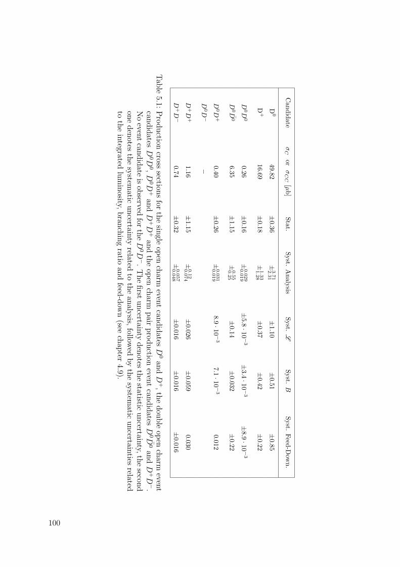
Can
did
ate
σC
orσCC
[µb
]S
tat.
Syst.
An
aly
sisS
yst.
LS
yst.
BS
yst.
Feed
-Dow
n.
D0
49.8
2±
0.36
±3.71
2.31
±1.1
0±
0.51±
0.85
D+
16.6
9±
0.18
±1.33
1.28
±0.3
7±
0.42±
0.22
D0D
00.26
±0.1
6±
0.029
0.019
±5.8·10−3
±3.4·10
−3
±8.9·10
−3
D0D
06.35
±1.1
5±
0.55
0.25
±0.1
4±
0.032±
0.22
D0D
+0.40
±0.2
6±
0.031
0.019
8.9·1
0−3
7.1·10
−3
0.012
D0D
−−
D+D
+1.1
6±
1.15
±0.12
0.074
±0.0
26
±0.059
0.030
D+D
−0.7
4±
0.32
±0.057
0.048
±0.0
16
±0.016
±0.016
Tab
le5.1:
Pro
duction
crosssection
sfor
the
single
open
charm
event
candid
atesD
0an
dD
+,
the
dou
ble
open
charm
event
candid
atesD
0D0,D
0D+
andD
+D
+an
dth
eop
ench
armpair
pro
duction
event
candid
atesD
0D0
andD
+D−
.N
oeven
tcan
did
ateis
observed
forth
eD
0D−
.T
he
first
uncertain
tyden
otesth
estatistic
uncertain
ty,th
esecon
don
eden
otesth
esy
stematic
uncertain
tyrelated
toth
ean
alysis,
followed
by
the
system
aticuncertain
tiesrelated
toth
ein
tegratedlu
min
osity,bran
chin
gratio
and
feed-d
own
(seech
apter
4.9).
100
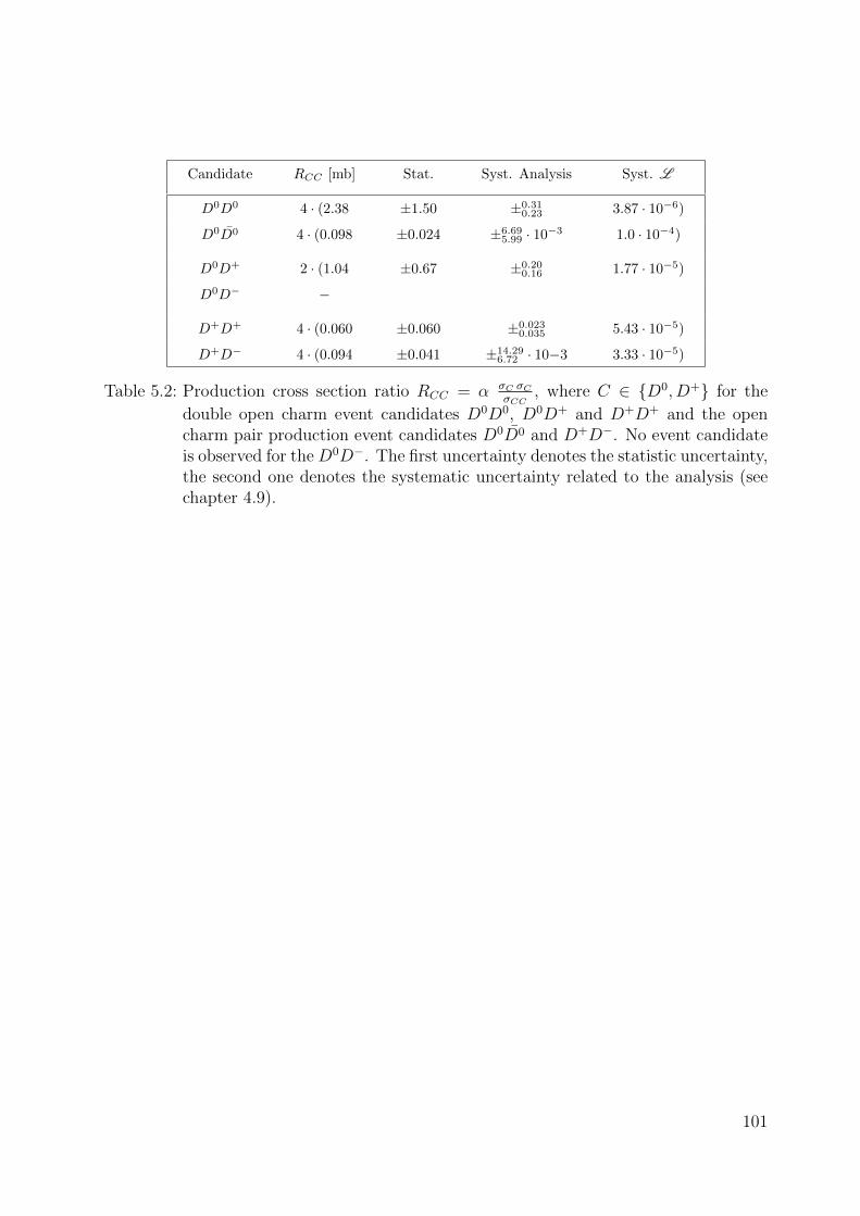
Candidate RCC [mb] Stat. Syst. Analysis Syst. L
D0D0 4 · (2.38 ±1.50 ±0.310.23 3.87 · 10−6)
D0D0 4 · (0.098 ±0.024 ±6.695.99 · 10−3 1.0 · 10−4)
D0D+ 2 · (1.04 ±0.67 ±0.200.16 1.77 · 10−5)
D0D− −
D+D+ 4 · (0.060 ±0.060 ±0.0230.035 5.43 · 10−5)
D+D− 4 · (0.094 ±0.041 ±14.296.72 · 10−3 3.33 · 10−5)
Table 5.2: Production cross section ratio RCC = α σC σCσCC
, where C ∈ {D0, D+} for the
double open charm event candidates D0D0, D0D+ and D+D+ and the opencharm pair production event candidates D0D0 and D+D−. No event candidateis observed for the D0D−. The first uncertainty denotes the statistic uncertainty,the second one denotes the systematic uncertainty related to the analysis (seechapter 4.9).
101
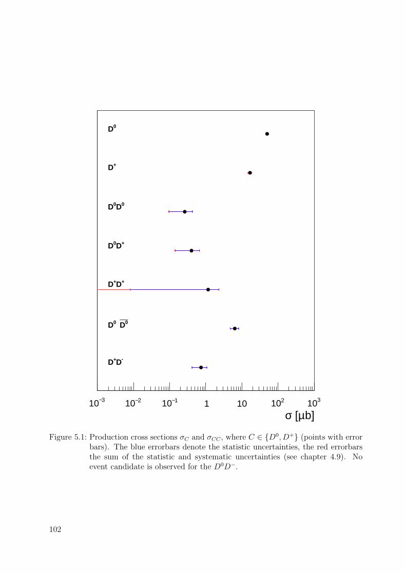
b]µ [σ3−10 2−10 1−10 1 10 210 310
0D
+D
0D0D
+D0D
+D+D
0D 0D
-D+D
Figure 5.1: Production cross sections σC and σCC , where C ∈ {D0, D+} (points with errorbars). The blue errorbars denote the statistic uncertainties, the red errorbarsthe sum of the statistic and systematic uncertainties (see chapter 4.9). Noevent candidate is observed for the D0D−.
102

b]µ [ABR1 10 210 310 410 510
0D0D
+D0D
+D+D
0D 0D
-D+D
Figure 5.2: Production cross section ratios RCC := α σC σCσCC
, where C ∈ {D0, D+} (pointswith error bars) in comparison with the measured effective cross section atTevatron for multi-jet events (green dotted). The blue errorbars denote thestatistic uncertainties, the red errorbars the sum of the statistic and systematicuncertainties. No event candidate is observed for the D0D−.
103
6 Conclusion and Outlook
The production of single and double open charm mesons have been seen in pp collisions at√s = 2.26 TeV. The signals are clearly visible in the mass distributions for the modes D0,
D+ and D0D0 but less obvious for the double open charm modes involving D+. A quan-titative determination of the statistical significance was not performed. Nevertheless, thisanalysis reuses techniques from previous analyses, that produced significant observations[2], [28].
Based on this signal, a cross section measurement is attempted. For each class of recon-structed candidates a cross section could be calculated and fully corrected for reconstruc-tion, tracking, particle identification, luminosity and branching ratio. However, a precisedetermination of the double open charm and pair production cross sections was not pos-sible due to few candidates. The integrated luminosity needs to be increased to be ableto do so. Moreover, the low and probably unprecisely determined charm trigger efficiencydoes not allow a precision measurement. In the LHCb collaboration, this is known to be adifficult problem.
Alternatively, a random trigger can be used especially for the D0 and D+ modes dueto their large cross section. For the double open charm production, asymmetric selectionsmay be feasible. Those would avoid using the charm trigger at low (pT , y), still allowingthe second charm meson to pass the selection. Also, data from 2012 taken at 8 TeV usingthe same trigger can be utilized. Combined with available random triggers, this might helpto improve the precision. For this work, this was not possible due to time constraints.
104

A Invariant Mass Fit Parameters
The fit parameters of the unbinned maximum likelihood fit to the invariant mass distribu-tions MC , where C ∈ {D0, D+} for the Gaussian, Bukin and Double Crystal Ball modelsare listed in Tab. A.1, A.2, A.3, respectively.
The fit parameters of the unbinned maximum likelihood fit to the invariant mass dis-tributions MCC , where CC ∈ {D0D0 ∪ D0D0, D0D+ ∪ D0D−, D+D+ ∪ D+D−} for theGaussian, Bukin and Double Crystal Ball models are listed in Tab. A.1, A.2, A.3, respec-tively.
Fit Parameter D0 D+
µ [GeV] 1.866± 2.9 · 10−5 1.871± 3.6 · 10−5
σ [GeV] (8.054± 0.024) · 10−3 (7.949± 0.031) · 10−3
NS 91006.7± 313.7 56141.3± 247.2
τ −13.969± 0.552 −13.022± 0.706
NB 5433.9± 113.4 3567.0± 92.4
Table A.1: Fit parameters of the unbinned maximum likelihood fit to the invariant massdistributions for the single open charm event candidates D0, D+, MD0 , MD+ ,using the Gaussian model.
105

Fit Parameter D0 D+
µ [GeV] 1.867± 3.1 · 10−5 1.871± 7.1 · 10−5
σ [GeV] (7.369± 0.028) · 10−3 (7.293± 0.027) · 10−3
ξ (−2.515± 0.122) · 10−3 (−5.561± 4.490) · 10−3
ρl −0.155± 0.012 −0.137± 0.001
ρr −0.232± 0.010 −0.232± 0.003
NS 92469.9± 308.5 57328.9± 242.4
τ −14.919± 0.919 −14.706± 1.220
NB 3915.4± 141.7 2201.7± 106.2
Table A.2: Fit parameters of the unbinned maximum likelihood fit to the invariant massdistributions for the single open charm event candidates D0, D+, MD0 , MD+ ,using the Bukin model.
Fit Parameter D0 D+
µ [GeV] 1.866± 3.3 · 10−5 1.871± 4.1 · 10−5
σ [GeV] (7.618± 0.035) · 10−3 (7.262± 0.048) · 10−3
αl 1.339± 0.047 0.946± 0.051
αr −1.259± 0.072 −1.321± 0.047
nl 65.098± 42.820 98.559± 0.306
nr 138.020± 0.217 146.362± 85.789
r 0.638± 0.060 0.407± 0.049
NS 92638.6± 309.3 57588.3± 243.7
τ −14.919± 0.919 −14.706± 1.220
NB 3915.4± 141.7 2201.7± 106.2
Table A.3: Fit parameters of the unbinned maximum likelihood fit to the invariant massdistributions for the single open charm event candidates D0, D+, MD0 , MD+ ,using the Double Crystal Ball model.
106
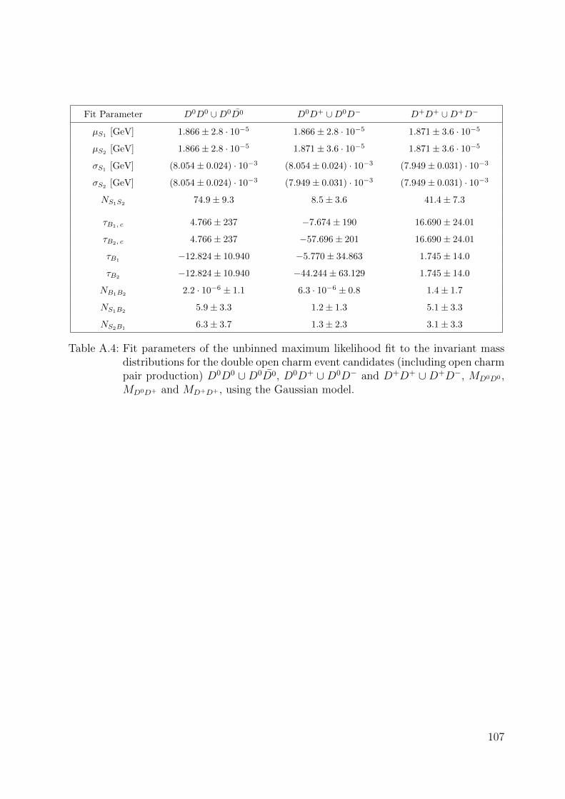
Fit Parameter D0D0 ∪D0D0 D0D+ ∪D0D− D+D+ ∪D+D−
µS1 [GeV] 1.866± 2.8 · 10−5 1.866± 2.8 · 10−5 1.871± 3.6 · 10−5
µS2 [GeV] 1.866± 2.8 · 10−5 1.871± 3.6 · 10−5 1.871± 3.6 · 10−5
σS1[GeV] (8.054± 0.024) · 10−3 (8.054± 0.024) · 10−3 (7.949± 0.031) · 10−3
σS2[GeV] (8.054± 0.024) · 10−3 (7.949± 0.031) · 10−3 (7.949± 0.031) · 10−3
NS1S2 74.9± 9.3 8.5± 3.6 41.4± 7.3
τB1, c 4.766± 237 −7.674± 190 16.690± 24.01
τB2, c 4.766± 237 −57.696± 201 16.690± 24.01
τB1−12.824± 10.940 −5.770± 34.863 1.745± 14.0
τB2−12.824± 10.940 −44.244± 63.129 1.745± 14.0
NB1B2 2.2 · 10−6 ± 1.1 6.3 · 10−6 ± 0.8 1.4± 1.7
NS1B2 5.9± 3.3 1.2± 1.3 5.1± 3.3
NS2B16.3± 3.7 1.3± 2.3 3.1± 3.3
Table A.4: Fit parameters of the unbinned maximum likelihood fit to the invariant massdistributions for the double open charm event candidates (including open charmpair production) D0D0 ∪D0D0, D0D+ ∪D0D− and D+D+ ∪D+D−, MD0D0 ,MD0D+ and MD+D+ , using the Gaussian model.
107

Fit Parameter D0D0 ∪D0D0 D0D+ ∪D0D− D+D+ ∪D+D−
µS1 [GeV] 1.867± 3.1 · 10−5 1.867± 3.1 · 10−5 1.871± 7.1 · 10−5
µS2 [GeV] 1.867± 3.1 · 10−5 1.871± 7.1 · 10−5 1.871± 7.1 · 10−5
σS1[GeV] (7.369± 0.028) · 10−3 (7.369± 0.028) · 10−3 (7.293± 0.027) · 10−3
σS2[GeV] (7.369± 0.028) · 10−3 (7.293± 0.027) · 10−3 (7.293± 0.027) · 10−3
ξS1 (−2.515± 0.122) · 10−3 (−2.515± 0.122) · 10−3 (−5.561± 4.490) · 10−3
ξS2 (−2.515± 0.122) · 10−3 (−5.561± 4.490) · 10−3 (−5.561± 4.490) · 10−3
ρl;S1−0.155± 0.012 −0.155± 0.012 −0.137± 0.001
ρl;S2−0.155± 0.012 −0.137± 0.001 −0.137± 0.001
ρr;S1 −0.232± 0.010 −0.232± 0.010 −0.232± 0.003
ρr;S2 −0.232± 0.010 −0.232± 0.003 −0.232± 0.003
NS1S278.1± 7.4 9.4± 3.7 44.3± 7.8
τB1, c −4.949± 245 −8.849± 173 1.227± 23.517
τB2, c −4.949± 245 −16.848± 157 1.227± 23.517
τB1 −8.437± 10.437 −4.961± 65.092 2.518± 20.798
τB2 −8.437± 10.437 −4.422± 61.592 2.518± 20.798
NB1B22.7 · 10−6 ± 183.0 1.3 · 10−6 ± 190.2 1.4± 1.9
NS1B24.0± 2.5 1.2± 1.2 4.3± 3.1
NS2B14.9± 2.7 0.4± 3.4 0.9± 5.0
Table A.5: Fit parameters of the unbinned maximum likelihood fit to the invariant massdistributions for the double open charm event candidates (including open charmpair production) D0D0 ∪D0D0, D0D+ ∪D0D− and D+D+ ∪D+D−, MD0D0 ,MD0D+ and MD+D+ , using the Bukin model.
108
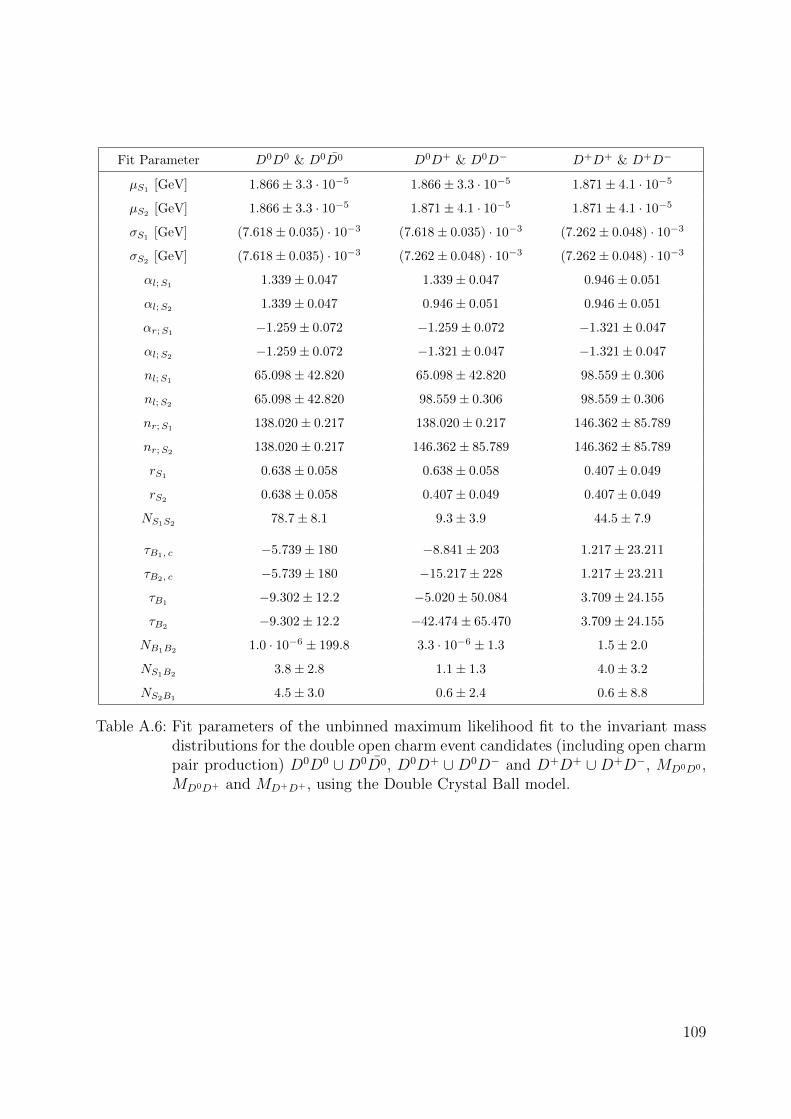
Fit Parameter D0D0 & D0D0 D0D+ & D0D− D+D+ & D+D−
µS1 [GeV] 1.866± 3.3 · 10−5 1.866± 3.3 · 10−5 1.871± 4.1 · 10−5
µS2 [GeV] 1.866± 3.3 · 10−5 1.871± 4.1 · 10−5 1.871± 4.1 · 10−5
σS1[GeV] (7.618± 0.035) · 10−3 (7.618± 0.035) · 10−3 (7.262± 0.048) · 10−3
σS2[GeV] (7.618± 0.035) · 10−3 (7.262± 0.048) · 10−3 (7.262± 0.048) · 10−3
αl;S1 1.339± 0.047 1.339± 0.047 0.946± 0.051
αl;S2 1.339± 0.047 0.946± 0.051 0.946± 0.051
αr;S1−1.259± 0.072 −1.259± 0.072 −1.321± 0.047
αl;S2−1.259± 0.072 −1.321± 0.047 −1.321± 0.047
nl;S1 65.098± 42.820 65.098± 42.820 98.559± 0.306
nl;S2 65.098± 42.820 98.559± 0.306 98.559± 0.306
nr;S1138.020± 0.217 138.020± 0.217 146.362± 85.789
nr;S2138.020± 0.217 146.362± 85.789 146.362± 85.789
rS1 0.638± 0.058 0.638± 0.058 0.407± 0.049
rS2 0.638± 0.058 0.407± 0.049 0.407± 0.049
NS1S278.7± 8.1 9.3± 3.9 44.5± 7.9
τB1, c −5.739± 180 −8.841± 203 1.217± 23.211
τB2, c −5.739± 180 −15.217± 228 1.217± 23.211
τB1−9.302± 12.2 −5.020± 50.084 3.709± 24.155
τB2 −9.302± 12.2 −42.474± 65.470 3.709± 24.155
NB1B21.0 · 10−6 ± 199.8 3.3 · 10−6 ± 1.3 1.5± 2.0
NS1B23.8± 2.8 1.1± 1.3 4.0± 3.2
NS2B14.5± 3.0 0.6± 2.4 0.6± 8.8
Table A.6: Fit parameters of the unbinned maximum likelihood fit to the invariant massdistributions for the double open charm event candidates (including open charmpair production) D0D0 ∪D0D0, D0D+ ∪D0D− and D+D+ ∪D+D−, MD0D0 ,MD0D+ and MD+D+ , using the Double Crystal Ball model.
109
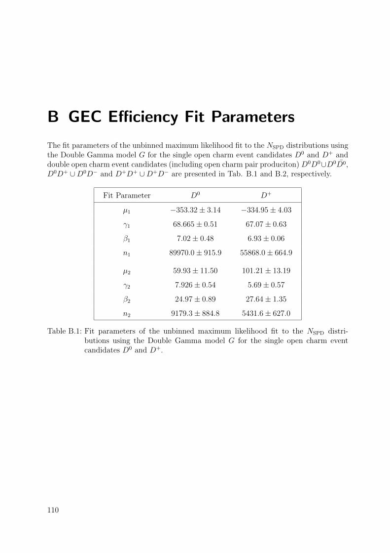
B GEC Efficiency Fit Parameters
The fit parameters of the unbinned maximum likelihood fit to the NSPD distributions usingthe Double Gamma model G for the single open charm event candidates D0 and D+ anddouble open charm event candidates (including open charm pair produciton) D0D0∪D0D0,D0D+ ∪D0D− and D+D+ ∪D+D− are presented in Tab. B.1 and B.2, respectively.
Fit Parameter D0 D+
µ1 −353.32± 3.14 −334.95± 4.03
γ1 68.665± 0.51 67.07± 0.63
β1 7.02± 0.48 6.93± 0.06
n1 89970.0± 915.9 55868.0± 664.9
µ2 59.93± 11.50 101.21± 13.19
γ2 7.926± 0.54 5.69± 0.57
β2 24.97± 0.89 27.64± 1.35
n2 9179.3± 884.8 5431.6± 627.0
Table B.1: Fit parameters of the unbinned maximum likelihood fit to the NSPD distri-butions using the Double Gamma model G for the single open charm eventcandidates D0 and D+.
110

Fit Parameter D0D0 ∪D0D0 D0D+ ∪D0D− D+D+ ∪D+D−
µ 15.77± 62.40 −1.63 · 10−3 ± 137 −10.57± 192
γ 4.64± 4.15 1.10± 4.89 5.74± 12.10
β 29.34± 13.90 16.79± 7.62 27.07± 2.86
n 86.0± 9.3 10.0± 3.2 51.0± 7.1
Table B.2: Fit parameters of the unbinned maximum likelihood fit to the NSPD distribu-tions using the Single Gamma model g for the double open charm event can-didates (including open charm pair production) D0D0 ∪D0D0, D0D+ ∪D0D−
and D+D+ ∪D+D−.
The fit parameters of the unbinned maximum likelihood fit to the NSPD distributionsusing the Single Gamma and Beta models for the single open charm event candidates D0
and D+ are presented in Tab. B.3 and B.4, respectively. For the Beta model a stretchedBeta PDF with a special representation for the mean µ and mode ν is used:
B(x; a, b) = nx
c
(xc
)−cµ+2 µνc(ν−µ)
−1 (1− x
c
)(−cµ+2 µνc(ν−µ)
−1)( cµ−1)−1
,
x : observable, i.e. NSPD for the single open charm event candidates
µ > 0, ν > 0 : mean and mode of the Beta PDF
n, c : normalization factors .
(B.1)
Fit Parameter D0 D+
µ −8.16± 2.81 −9.68± 3.93
γ 5.36± 0.17 5.70± 0.26
β 28.72± 0.46 27.20± 0.61
n 96095.6± 361.3 59613.6± 282.8
Table B.3: Fit parameters of the unbinned maximum likelihood fit to the NSPD distribu-tions using the Single Gamma model for the single open charm event candidatesD0 and D+.
111
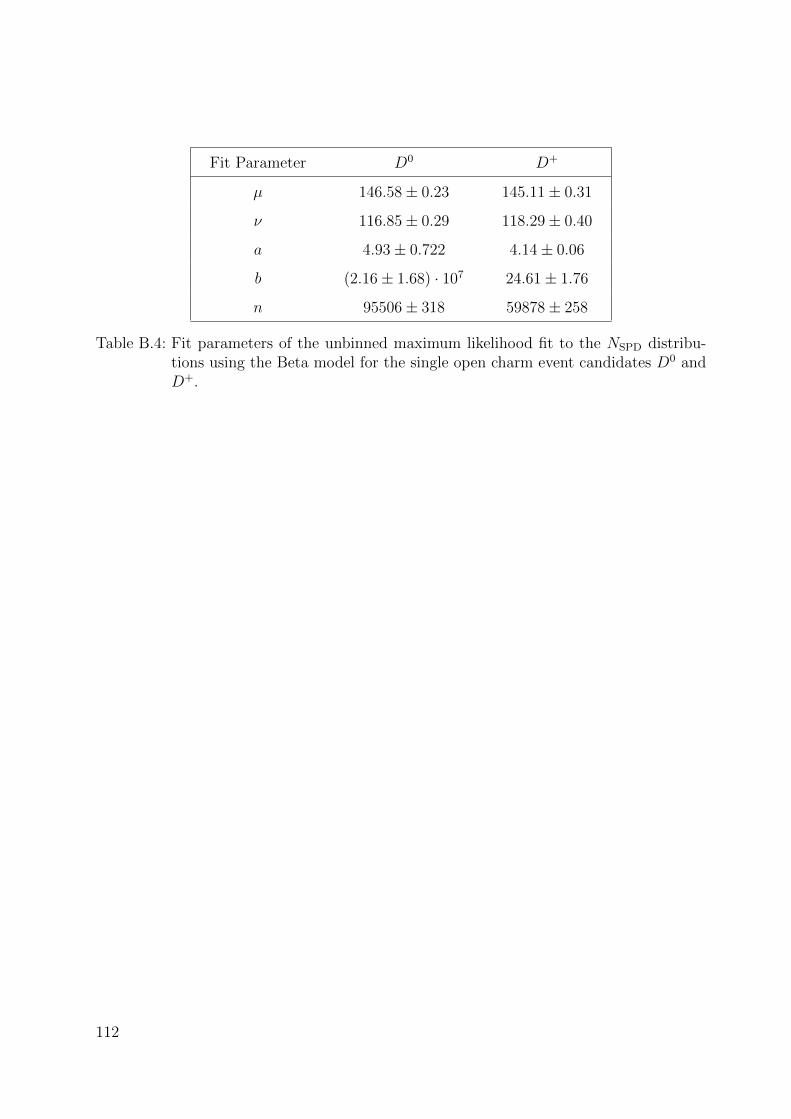
Fit Parameter D0 D+
µ 146.58± 0.23 145.11± 0.31
ν 116.85± 0.29 118.29± 0.40
a 4.93± 0.722 4.14± 0.06
b (2.16± 1.68) · 107 24.61± 1.76
n 95506± 318 59878± 258
Table B.4: Fit parameters of the unbinned maximum likelihood fit to the NSPD distribu-tions using the Beta model for the single open charm event candidates D0 andD+.
112
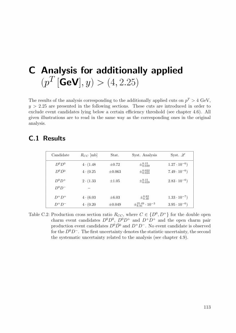
C Analysis for additionally applied(pT [GeV], y) > (4, 2.25)
The results of the analysis corresponding to the additionally applied cuts on pT > 4 GeV,y > 2.25 are presented in the following sections. These cuts are introduced in order toexclude event candidates lying below a certain efficiency threshold (see chapter 4.6). Allgiven illustrations are to read in the same way as the corresponding ones in the originalanalysis.
C.1 Results
Candidate RCC [mb] Stat. Syst. Analysis Syst. L
D0D0 4 · (1.48 ±0.72 ±0.150.039 1.27 · 10−6)
D0D0 4 · (0.25 ±0.063 ±0.0220.024 7.49 · 10−6)
D0D+ 2 · (1.33 ±1.05 ±0.150.029 2.83 · 10−6)
D0D− −
D+D+ 4 · (6.03 ±6.03 ±0.820.30 1.33 · 10−7)
D+D− 4 · (0.20 ±0.049 ±25.498.91 · 10−3 3.95 · 10−6)
Table C.2: Production cross section ratio RCC , where C ∈ {D0, D+} for the double opencharm event candidates D0D0, D0D+ and D+D+ and the open charm pairproduction event candidates D0D0 and D+D−. No event candidate is observedfor the D0D−. The first uncertainty denotes the statistic uncertainty, the secondthe systematic uncertainty related to the analysis (see chapter 4.9).
113
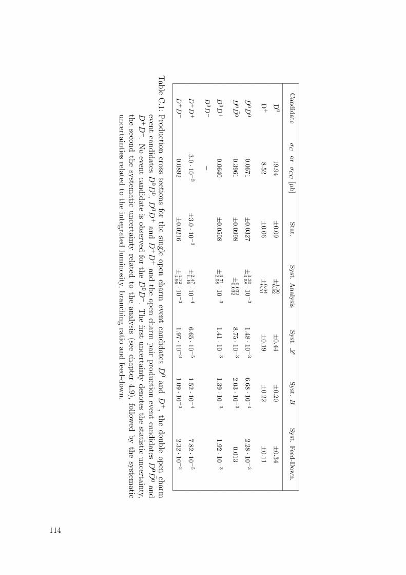
Can
did
ateσC
orσCC
[µb
]S
tat.
Syst.
An
aly
sisS
yst.
LS
yst.
BS
yst.
Feed
-Dow
n.
D0
19.94
±0.0
9±
1.30
0.82
±0.4
4±
0.20
±0.34
D+
8.52±
0.0
6±
0.64
0.51
±0.1
9±
0.22
±0.11
D0D
00.067
1±
0.0327
±3.20
3.58 ·1
0−3
1.4
8·1
0−3
6.68·10
−4
2.28·10
−3
D0D
00.3
961±
0.0998
±0.032
0.032
8.7
5·1
0−3
2.03·10
−3
0.013
D0D
+0.0
640±
0.0508
±3.71
2.58 ·1
0−3
1.4
1·1
0−3
1.39·10
−3
1.92·10
−3
D0D
−−
D+D
+3.0·10
−3
±3.0·1
0−3
±2.47
1.16 ·1
0−4
6.6
5·1
0−5
1.52·10
−4
7.82·10
−5
D+D
−0.0
892±
0.0216
±4.72
4.96 ·1
0−3
1.9
7·1
0−3
1.09·10
−3
2.32·10
−3
Tab
leC
.1:P
roduction
crosssection
sfor
the
single
open
charm
event
candid
atesD
0an
dD
+,
the
dou
ble
open
charm
event
candid
atesD
0D0,D
0D+
andD
+D
+an
dth
eop
ench
armpair
pro
duction
event
candid
atesD
0D0
and
D+D−
.N
oeven
tcan
did
ateis
observed
forth
eD
0D−
.T
he
first
uncertain
tyden
otesth
estatistic
uncertain
ty,th
esecon
dth
esy
stematic
uncertain
tyrelated
toth
ean
alysis
(seech
apter
4.9),follow
edby
the
system
aticuncertain
tiesrelated
toth
ein
tegratedlu
min
osity,bran
chin
gratio
and
feed-d
own.
114

b]µ [σ3−10 2−10 1−10 1 10 210 310
0D
+D
0D0D
+D0D
+D+D
0D 0D
-D+D
Figure C.1: Production cross sections σC and σCC , where C ∈ {D0, D+} (points with errorbars). The blue errorbars denote the statistic uncertainties, the red errorbarsthe sum the statistic and systematic uncertainties (see chapter 4.9). No eventcandidate is observed for the D0D−.
115

b]µ [ABR1 10 210 310 410 510
0D0D
+D0D
+D+D
0D 0D
-D+D
Figure C.2: Production cross section ratios RCC := α σC σCσCC
, where C ∈ {D0, D+} (pointswith error bars) in comparison with the measured effective cross section atTevatron for multi-jet events (green dotted). The blue errorbars denote thestatistic uncertainties, the red errorbars the sum of the statistic and systematicuncertainties (see chapter 4.9). No event candidate is observed for the D0D−
116

C.2 Systematic Uncertainties
b]µ [0Dσ
16 18 20 22 24 26 28 30
/ B
injn
0
10
20
30
40
50
60
Stat. Values
bµMean = 20.21
bµRMS = 1.14
bµMode = 19.74
bµMedian = 20.18
bµBest Value = 23.32
bµLower Bound = 18.92
bµUpper Bound = 21.04
b]µ [+Dσ6 7 8 9 10 11 12 13 14 15 16
/ B
injn
0
10
20
30
40
50
60
70
80
Stat. Values
bµMean = 8.82
bµRMS = 0.79
bµMode = 8.58
bµMedian = 8.65
bµBest Value = 9.62
bµLower Bound = 8.08
bµUpper Bound = 9.23
Figure C.3: Cross section distributions obtained from the toy experiments for the singleopen charm event candidates D0 (left) and D+ (right). The mode of a distri-butions is denoted as Mode and drawn as a red star, while the cross sectionvalue calculated by the analysis is denoted as Best V alue and drawn as greentriangle. The parameters LowerBound and UpperBound correspond to thelower and upper end points of the error bar, drawn in pink. The other statisticsparameter calculated from the binned distributions are the mean, median andstandard deviation, denoted as Mean, Median and RMS.
117

b]µ [0D0Dσ
0.02 0.03 0.04 0.05 0.06 0.07 0.08 0.09 0.1
/ B
injn
0
20
40
60
80
100
Stat. Values
bµMean = 0.07
bµRMS = 0.00
bµMode = 0.07
bµMedian = 0.07
bµBest Value = 0.07
bµLower Bound = 0.06
bµUpper Bound = 0.07
b]µ [0D0Dσ
0.3 0.4 0.5 0.6 0.7 0.8 0.9 1 1.1 1.2
/ B
injn
0
20
40
60
80
100
120
140
Stat. Values
bµMean = 0.43
bµRMS = 0.08
bµMode = 0.40
bµMedian = 0.40
bµBest Value = 0.43
bµLower Bound = 0.36
bµUpper Bound = 0.43
b]µ [+D0Dσ
0.05 0.055 0.06 0.065 0.07 0.075 0.08 0.085
/ B
injn
0
10
20
30
40
50
60
Stat. Values
bµMean = 0.06
bµRMS = 0.00
bµMode = 0.06
bµMedian = 0.06
bµBest Value = 0.07
bµLower Bound = 0.06
bµUpper Bound = 0.07
b]µ [+D+Dσ0.0024 0.0026 0.0028 0.003 0.0032 0.0034 0.0036 0.0038 0.004
/ B
injn
0
5
10
15
20
25
30
35
40
Stat. Values
bµMean = 0.00
bµRMS = 0.00
bµMode = 0.00
bµMedian = 0.00
bµBest Value = 0.00
bµLower Bound = 0.00
bµUpper Bound = 0.00
b]µ [-D+Dσ0.07 0.075 0.08 0.085 0.09 0.095 0.1 0.105 0.11 0.115 0.12
/ B
injn
0
10
20
30
40
50
Stat. Values
bµMean = 0.09
bµRMS = 0.01
bµMode = 0.09
bµMedian = 0.09
bµBest Value = 0.09
bµLower Bound = 0.09
bµUpper Bound = 0.10
Figure C.4: Cross section distributions obtained from the toy experiments for the doubleopen charm event candidates D0D0 (top left), D0D+ (center left), D+D+
(bottom left) and for the open charm pair production event candidates D0D0
(top right) and D+D− (bottom right). No event candidate is observed forthe D0D−. The mode of a distributions is denoted as Mode and drawn as ared star, while the cross section value calculated by the analysis is denotedas Best V alue and drawn as green triangle. The parameters LowerBoundand UpperBound correspond to the lower and upper end points of the errorbar, drawn in pink. The other statistics parameter calculated from the binneddistributions are the mean, median and standard deviation, denoted as Mean,Median and RMS.
118
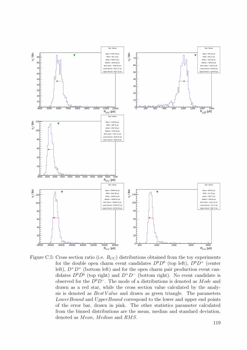
b]µ [0D0DR4000 5000 6000 7000 8000 9000 10000 11000 12000
/ B
injn
0
10
20
30
40
50
60
70
80
90
Stat. Values
bµMean = 6057.93
bµRMS = 461.11
bµMode = 5828.14
bµMedian = 6040.00
bµBest Value = 7666.94
bµLower Bound = 5670.17
bµUpper Bound = 6427.23
b]µ [0D0DR
0 200 400 600 800 1000 1200 1400 1600
/ B
injn
0
10
20
30
40
50
60
70
Stat. Values
bµMean = 961.95
bµRMS = 162.12
bµMode = 1014.95
bµMedian = 1000.00
bµBest Value = 1256.24
bµLower Bound = 918.93
bµUpper Bound = 1104.64
b]µ [+D0DR2000 2500 3000 3500 4000 4500 5000 5500 6000 6500 7000
/ B
injn
0
20
40
60
80
100
120
Stat. Values
bµMean = 2758.55
bµRMS = 298.70
bµMode = 2587.83
bµMedian = 2725.00
bµBest Value = 3227.67
bµLower Bound = 2529.34
bµUpper Bound = 2881.66
b]µ [+D+DR10000 20000 30000 40000 50000 60000 70000 80000
/ B
injn
0
20
40
60
80
100
120
Stat. Values
bµMean = 25584.46
bµRMS = 4421.95
bµMode = 23444.01
bµMedian = 25050.00
bµBest Value = 30494.15
bµLower Bound = 22253.22
bµUpper Bound = 26743.94
b]µ [-D+DR500 1000 1500 2000 2500
/ B
injn
0
20
40
60
80
100
120
Stat. Values
bµMean = 859.35
bµRMS = 147.18
bµMode = 786.77
bµMedian = 829.00
bµBest Value = 1013.15
bµLower Bound = 751.15
bµUpper Bound = 888.72
Figure C.5: Cross section ratio (i.e. RCC) distributions obtained from the toy experimentsfor the double open charm event candidates D0D0 (top left), D0D+ (centerleft), D+D+ (bottom left) and for the open charm pair production event can-didates D0D0 (top right) and D+D− (bottom right). No event candidate isobserved for the D0D−. The mode of a distributions is denoted as Mode anddrawn as a red star, while the cross section value calculated by the analy-sis is denoted as Best V alue and drawn as green triangle. The parametersLowerBound and UpperBound correspond to the lower and upper end pointsof the error bar, drawn in pink. The other statistics parameter calculatedfrom the binned distributions are the mean, median and standard deviation,denoted as Mean, Median and RMS.
119
References
[1] R. Maciula and A. Szczurek, Production of cccc in single and double parton scatteringin collinear and kt-factorization approaches, PoS EPS-HEP2015 (2015) 500.
[2] The LHCb Collaboration, R. Aaij et al., Observation of double charm productioninvolving open charm in pp collisions at
√s = 7 TeV, JHEP 06 (2012) 141 Addendum
ibid. 03 (2014) 108, arXiv:1205.0975.
[3] A. Artamonov, V. Belyaev, V. Egorychev, D. Golubkov, J. He, A. Kozlinskiy, M.Needham, A. Novoselov and V. Romanovskiy, Observation of J/ψ, open charm anddouble open charm production in pp collisions at
√s = 7 TeV, LHCB-ANA-2011-067.
[4] M. Peskin and D. Schroder, An Introduction to Quantum Field Theory, AdvancedBook Program (ABP), Westview Press, Boulder, Colorado, October 1995.
[5] S. Weinberg, The Quantum Theory of Fields, Cambridge University Press, Cambridge,UK, 2005.
[6] J. Horejsi, Fundamentals of Electroweak Theory, The Karolinum Press, Charles Uni-versity in Prague, Prague, Chech, 2002.
[7] Particle Data Group Collaboration, K. A. Olive et al., Review of Particle Physics,Chin. Phys. C, 38, 090001 (2014) and 2015 update.
[8] The LHCb Collaboration, R. Aaij et al., Prompt charm production in pp collisions at√s = 7 TeV, Nucl. Phys. B 871 (2013) 1-20, arXiv:1302.2864.
[9] J. Collins, D. Soper and G. Sterman, Factorization of Hard Processes in QCD, Adv.Ser. Direct. High Energy Phys. 5 (1989) 1-91, arXiv:hep-ph/0409313.
[10] J. R. Gault, C. -H. Kom, A. Kulesza and W. J. Stirling, Same-sign W pair productionas a probe of double-parton scattering at the LHC, Eur. Phys. J. C 69 (2010) 53-65,arXiv:1003.3953 [hep-ph].
[11] H. D. Politzer, Power Corrections at Short Distances, Nucl. Phys. B 172 (1980) 349-382.
[12] N. Paver and D. Treleani, Multi-Quark Scattering and Large pT Jet Production inHadronic Collisions, Nuovo Cim. A 70 (1982) 215.
120

[13] M. Rinaldi, S. Scopetta and V. Vento, Double parton correlations in constituent quarkmodels, Phys. Rev. D 87 (2013) 114021, arXiv:1302.6462 [hep-ph].
[14] M. H. Seymour and A. Siodmok, Constraining MPI models using σeff and recent Teva-tron and LHC underlying event data, JHEP 1310 (2013) 113, arXiv:1307.5015 [hep-ph].
[15] M. H. Seymour and A. Siodmok, Extracting σeffective from the LHCb double charmmeasurement, MAN-HEP-2013-20, MC-NET-13-11, arXiv:1308.6749 [hep-ph].
[16] The CDF Collaboration, F. Abe et al., Double parton scattering in pp collisions at√s = 1.8 TeV, Phys. Rev. D 56 (1997) 3811-3832.
[17] The Axial Field Spectrometer Collaboration, T. Akesson et al., Double Parton Scat-terin in pp Collisions at
√s = 63 GeV, Z. Phys. C 34 (1987) 163.
[18] L. Kowarski, An account of the origin and beginnings of CERN, CERN-61-10(see also: The History of CERN, http://timeline.web.cern.ch/timelines/The-history-of-CERN).
[19] L. Evans and P. Bryant, LHC Machine, JINST 3 (2008) S08001.
[20] L. Evans, The Large Hadron Collider: A Marvel of Technology, 1st edition, Funda-mental Sciences, CERN and EPFL Press, Lausanne 2009.
[21] C. Lefevre, LHC: the guide, CERN-Brochure-2009-003-Eng, March 2009.
[22] The LHCb Collaboration, A. Alves Jr. et al., The LHCb Detector at the LHC, JINST3 (2008) S08005.
[23] The LHCb Collaboration, R. Aaij et al., LHCb detector performance, Int. J. Mod.Phys. A 30 (2015) no. 07, 1530022, arXiv:1412.6352 [hep-ex].
[24] H. Goldstein, C. P. Poole Jr and J. L. Safko Sen., Classical Mechanics, 3rd edition,Addison-Wesley, San Francisco, June 25, 2001.
[25] U. Straumann, Relativitatstheorie: Erganzendes Skriptum zur Vorlesung Physik II,Physik-Institut Universitat Zurich, URL: http://www.physik.uzh.ch/∼straumann/physik-a/srt.pdf, Marz 2013.
[26] J. W. Barlow, Statistics: A Guide to the Use of Statistical Methods in the PhysicalSciences, 6th edition, John Wiley & Sons, New York, July 1999.
[27] W. Stahel, Statistische Datenanalyse: Eine Einfuhrung fur Naturwissenschaftler, 4.Auflage, Springer Verlag, November 2002.
[28] The LHCb Collaboration, R. Aaij et al., Production of associated Υ and open charmhadrons in pp collisions at
√s = 7 and 8 TeV via double parton scattering, LHCB-
PAPER-2015-046, arXiv:1510.05949 [hep-ex].
121
[29] I. Belyaev, V. Egorychev, M. Needham and V. Romanovsky, Observation of the asso-ciative production of bottonimum and open charm mesons, LHCB-ANA-2013-063.
[30] S. Kullback and R. A. Leibler, On Information and Sufficiency, The Annals of Math-ematical Statistics Vol. 22, No. 1 (1951) 79-86.
[31] S. Kullback, Information Theory and Statistics, John Wiley and Sons, New York,USA, 1959.
[32] S. Kullback, Letters to the editor: the Kullback-Leibler distance, The American Sta-tistican Vol. 41, No. 4 (1987) 338-341.
[33] W. Hulsbergen, Decay chain fitting with a Kalman filter, Nucl. Instrum. Meth. A 552(2005) 566, arXiv:physics/0503191 [physics.comp-ph].
[34] The LHCb Collaboration, R. Aaij et al., Observation of associated production of a Zboson with a D meson in the forward region, JHEP 1404 (2014) 091, arXiv:1401.3235[hep-ex].
[35] I. Belyaev, A. Bursche and K. Muller, Observation of Z plus Charmed Hadron Pro-duction, LHCB-ANA-2013-047.
[36] R. Brun and F. Rademakers, ROOT: An object orientated data analysis framework,Proceedings AIHENP’96 Workshop, Lausanne, Nucl. Inst. & Meth. in Phys. Res. A389 (1997) 81-86 (see also http://root.cern.ch/).
[37] M. Pivk and F. Le Diberder, sPlot: A statistical tool to unfold data distributions, Nucl.Instrum. Meth. A 555 (2005) 356-369, arXiv:physics/0402083 [physics.data-an].
[38] The LHCb Collaboration, M. Clemencic et al., The LHCb simulation application,Gauss: Design, evolution and experience, J. Phys. Conf. Ser. 331 (2011) 032023.
[39] The LHCb Collaboration, I. Belyaev et al., Handling the generation of primary eventsin Gauss, the LHCb simulation framework, J. Phys. Conf. Ser. 331 032047(see also Nulear Science Symposium Conference Record (NSS/MIC) IEEE (2010)1155).
[40] The LHCb Collaboration, R. Aaij et al., Measurement of the track reconstructionefficiency at LHCb, JINST 10 (2015) no. 02, P02007, arXiv:1408.1251 [hep-ex].
[41] The LHCb Tracking Group, General LHCb Tracking Wiki Page,https://twiki.cern.ch/twiki/bin/view/LHCb/LHCbTracking.
[42] The LHCb RICH collaboration, M. Adinolfi et al., Performance of the LHCb RICHdetector at the LHC, Eur. Phys. J. C 73 (2013) 2431, arXiv:1211.6759 [physics.ins-det].
122
[43] The LHCb RICH collaboration, A. Powell for the collaboration, Reconstruction andPID performance of the LHCb RICH detectors, Nucl. Inst. Meth. A 639 (2011) 260-263.
[44] The LHCb collaboration, A. Powell for the collaboration, Particle identification atLHCb, PoS (ICHEP2010) 020, LHCb-PROC-2011-008.
[45] S. Malde, PID Calib Packages, https://twiki.cern.ch/twiki/bin/view/LHCb/PIDCalibPackage
[46] The LHCb collaboration, R. Aaij et al., Prompt K0s production in pp collisions at√
s = 0.9 TeV, Phys. Lett. B 693 (2010) 69, arXiv:1008.3105 [hep-ex].
[47] The LHCb collaboration, R. Aaij et al., Observation of J/ψ pair production in ppcollisions at
√s = 7 TeV, Phys. Lett. B 707 (2012) 52-59, arXiv:1109.0963.
[48] E. Lopez Azamar et al., Measurement of trigger efficiencies and biases, CERN- LHCb-2008-073.
[49] R. Aaij et al., The LHCb Trigger and its Performance in 2011, JINST 8 (2013) P04022,arXiv:1211.3055 [hep-ex].
[50] R. Puig, The LHCb trigger in 2011 and 2012, LHCb-PUB-2014-046.
[51] M. Vesterinen, LHCb trigger twiki pages, https://twiki.cern.ch/twiki/bin/view/LHCb/LHCbTrigger.
[52] C. J. Clopper and E. S. Pearson, The Use of Confidence or Fiducial Limits Illustratedin the Case of the Binomial, Biometrika Vol. 26, No. 4 (1934), pp. 404-413.
[53] The LHCb Collaboration, R. Aaij et al., Absolute luminosity measurements with theLHCb detector at the LHC, JINST 7 (2012) P01010, arXiv:1110.2866 [hep-ex].
[54] M. Ferro-Luzzi, Proposal for an absolute luminosity determination in colliding beamexperiments using vertex detection of beam-gas interactions, Nucl. Instrum .Meth. A553 (2005) 388-399.
[55] The LHCb Collaboration, R. Aaij et al., Precision luminosity measurements at LHCb,JINST 9 (2014) no. 12, P12005, arXiv:1410.0149 [hep-ex].
123