Embed Size (px)
Citation preview

Measurement and Verification Operational GuideWhole Building Applications

© Copyright State of NSW and Office of Environment and Heritage
With the exception of photographs, the State of NSW and Office of Environment and Heritage are pleased to allow this material to be reproduced in whole or in part for educational and non-commercial use, provided the meaning is unchanged and its source, publisher and authorship are acknowledged. Specific permission is required for the reproduction of photographs.
The Office of Environment and Heritage (OEH) has compiled this guideline in good faith, exercising all due care and attention. No representation is made about the accuracy, completeness or suitability of the information in this publication for any particular purpose. OEH shall not be liable for any damage which may occur to any person or organisation taking action or not on the basis of this publication. Readers should seek appropriate advice when applying the information to their specific needs.
Every effort has been made to ensure that the information in this document is accurate at the time of publication. However, as appropriate, readers should obtain independent advice before making any decision based on this information.
Published by: Office of Environment and Heritage NSW 59 Goulburn Street, Sydney NSW 2000 PO Box A290, Sydney South NSW 1232 Phone: (02) 9995 5000 (switchboard) Phone: 131 555 (environment information and publications requests) Phone: 1300 361 967 (national parks, climate change and energy efficiency information, and publications requests) Fax: (02) 9995 5999 TTY: (02) 9211 4723 Email: [email protected] Website: www.environment.nsw.gov.au
Report pollution and environmental incidents Environment Line: 131 555 (NSW only) or [email protected] See also www.environment.nsw.gov.au
ISBN 978 1 74293 959 9 OEH 2012/0993 December 2012
Printed on environmentally sustainable paper

Table of contents
i
Contents 1 Your guide to successful M&V projects ............................................................................ 1
1.1 Using the M&V Operational Guide ................................................................................. 1 1.2 The Whole Building Applications (this guide) ................................................................ 2
2 Understanding M&V concepts ........................................................................................... 4 2.1 Introducing key M&V terms ............................................................................................ 4 2.2 Best practise M&V process ............................................................................................ 5
3 Getting started ..................................................................................................................... 6 3.1 Proposed whole building ECM(s)................................................................................... 6 3.2 Decide approach for pursuing M&V ............................................................................... 8
4 M&V design and planning ................................................................................................... 9 4.1 M&V design .................................................................................................................... 9 4.2 Prepare M&V plan ........................................................................................................ 11
5 Data collection, modelling and analysis ......................................................................... 12 5.1 Measure baseline data ................................................................................................. 12 5.2 Develop energy model and uncertainty ....................................................................... 12 5.3 Implement ECM(s) ....................................................................................................... 13 5.4 Measure post retrofit data ............................................................................................ 13 5.5 Savings analysis and uncertainty................................................................................. 13
6 Finish .................................................................................................................................. 15 6.1 Reporting ...................................................................................................................... 15 6.2 Project close and savings persistence ......................................................................... 15
7 M&V Examples ................................................................................................................... 16 7.1 Examples from the IPMVP ........................................................................................... 16 7.2 Examples from this guide ............................................................................................. 17
Appendix A: Example scenario A – food processing plant .................................................. 18 Getting started ..................................................................................................................... 19 Summary of M&V plan ......................................................................................................... 20 Baseline model development .............................................................................................. 21 Developing the energy model for electricity......................................................................... 22 Validating the regression outputs ........................................................................................ 24 Developing the energy model for natural gas ...................................................................... 29 Calculating combined energy savings and uncertainty ....................................................... 33 Reporting results .................................................................................................................. 34
Appendix B: Example scenario B – commercial building ..................................................... 35 Getting started ..................................................................................................................... 35 Summary of M&V plan ......................................................................................................... 36 Baseline model development .............................................................................................. 37 Calculating electricity savings from Model 1 ........................................................................ 44 Uncertainty analysis for Model 1 ......................................................................................... 46 Reporting results from Model 1 ........................................................................................... 46 Reporting results from Model 2 ........................................................................................... 47


Your guide to successful M&V projects
1
1.1
1 Your guide to successful M&V projects The Measurement and Verification (M&V) Operational Guide has been developed to help M&V practitioners, business energy savings project managers, government energy efficiency program managers and policy makers translate M&V theory into successful M&V projects.
By following this guide you will be implementing the International Performance Measurement and Verification Protocol (IPMVP) across a typical M&V process. Practical tips, tools and scenario examples are provided to assist with decision making, planning, measuring, analysing and reporting outcomes.
But what is M&V exactly?
M&V is the process of using measurement to reliably determine actual savings for energy, demand, cost and greenhouse gases within a site by an Energy Conservation Measure (ECM). Measurements are used to verify savings, rather than applying deemed savings or theoretical engineering calculations, which are based on previous studies, manufacturer-provided information or other indirect data. Savings are determined by comparing post-retrofit performance against a ‘business as usual’ forecast.
Across Australia the use of M&V has been growing, driven by business and as a requirement in government funding and financing programs. M&V enables: § calculation of savings for projects that have high uncertainty or highly variable characteristics § verification of installed performance against manufacturer claims § a verified result which can be stated with confidence and can prove return on investment § demonstration of performance where a financial incentive or penalty is involved § effective management of energy costs § the building of robust business cases to promote successful outcomes
In essence, Measurement and Verification is intended to answer the question, “how can I be sure I’m really saving money?1”
1.1 Using the M&V Operational Guide The M&V Operational Guide is structured in three main parts; Process, Planning and Applications.
Process Guide: The Process Guide provides guidance that is common across all M&V projects. Practitioners new to M&V should start with the Process Guide to gain an understanding of M&V theory, principles, terminology and the overall process.
Planning Guide: The Planning Guide is designed to assist both new and experienced practitioners to develop a robust M&V Plan for your energy savings project, using a step-by-step process for designing a M&V project. A Microsoft Excel tool is also available to assist practitioners to capture the key components for a successful M&V Plan.
Applications Guides: Seven separate application-specific guides provide new and experienced M&V practitioners with advice, considerations and examples for technologies found in typical commercial and industrial sites. The Applications Guides should be used in conjunction with the Planning Guide to understand application-specific considerations and design choices. Application Guides are available for.
1 Source: www.energymanagementworld.org

Measurement and Verification Operational Guide
2
1.2
Application Guides are available for: § Lighting § Motors, pumps and fans § Commercial heating, ventilation and cooling § Commercial and industrial refrigeration § Boilers, steam and compressed air § Whole buildings § Renewables and cogeneration
Figure 1: M&V Operational Guide structure
1.2 The Whole Building Applications (this guide) The Whole Building Applications Guide provides specific guidance for conducting M&V for large and/or multiple projects throughout a site. It is designed to be used in conjunction with the Process Guide, providing tips, suggestions and examples specific to conducting evaluation using a facility boundary.

Your guide to successful M&V projects
3
1.2
The Whole Building Applications Guide is presented as follows:
§ Understanding M&V concepts Section 2 presents a high level diagram of the best practise M&V process.
§ Getting started Section 3 provides a discussion on key things that need to be considered when getting your M&V project started.
§ M&V design and planning Section 4 provides guidance on how to design and plan your whole building M&V project and key considerations, potential issues and suggested approaches.
§ Data collection, modelling and analysis Section 5 provides guidance on data collection, modelling and analysis for your whole building M&V project.
§ Finish Section 6 provides a discussion on reporting M&V outcomes, ongoing M&V and ensuring savings persist over time.
§ References to examples of M&V projects Section 7 provides a reference list of example projects located within the IPMVP and throughout this guide.
§ Example whole building scenario A Appendix A illustrates the M&V process using a worked example of a food processing plant project
§ Example whole building scenario B Appendix B illustrates the M&V process using a worked example of a commercial building project

Measurement and Verification Operational Guide
4
2.1
2 Understanding M&V concepts
2.1 Introducing key M&V terms The terms listed in Table 1 below are used throughout this guide and are introduced here to assist with initial understanding. Refer to Section 4 within the Process Guide for a full definition and explanation.
Table 1: Key M&V terms
M&V Term Definition Examples
Measurement boundary
A notional boundary that defines the physical scope of a M&V project. The effects of an ECM are determined at this boundary.
Whole facility, sub facility, lighting circuit, mechanical plant room, switchboard, individual plant and equipment etc.
Energy use Energy used within the measurement boundary.
Electricity, natural gas, LPG, transport fuels, etc
Key parameters Data sources relating to energy use and independent variables that are measured or estimated which form the basis for savings calculations.
Instantaneous power draw, metered energy use, efficiency, operating hours, temperature, humidity, performance output etc.
M&V Options Four generic approaches for conducting M&V which are defined within the IPMVP.
These are known as Options A, B, C and D.
Routine adjustments
Routine adjustments to energy use that are calculated based on analysis of energy use in relation to independent variables.
Energy use may be routinely adjusted based on independent variables such as ambient temperature, humidity, occupancy, business hours, production levels, etc.
Non routine adjustments
Once-off or infrequent changes in energy use or demand that occur due to changes in static factors
Energy use may be non routinely adjusted based on static factors such as changes to building size, facade, installed equipment, vacancy, etc. Unanticipated events can also temporarily or permanently affect energy use. Examples include natural events such as fire, flood, drought or other events such as equipment failure, etc.
Interactive effects
Changes in energy use resulting from an ECM which will occur outside our defined measurement boundary.
Changes to the HVAC heat load through lighting efficiency upgrades, interactive effects on downstream systems due to changes in motor speed/pressure/flow, etc.
Performance Output performance affected by the ECM.
System/equipment output (e.g. compressed air), comfort conditions, production, light levels, etc.

Understanding M&V concepts
5
2.2
2.2 Best practise M&V process The following figure presents the best practise M&V process which is how the rest of the Whole Building Applications Guide is structured. Refer to the Process Guide for detailed guidance on the M&V processes.
Figure 2: Best practise M&V process with references to M&V Process Guide
Measurement and Verification Operational Guide
6
3.1
3 Getting started
3.1 Proposed whole building ECM(s)
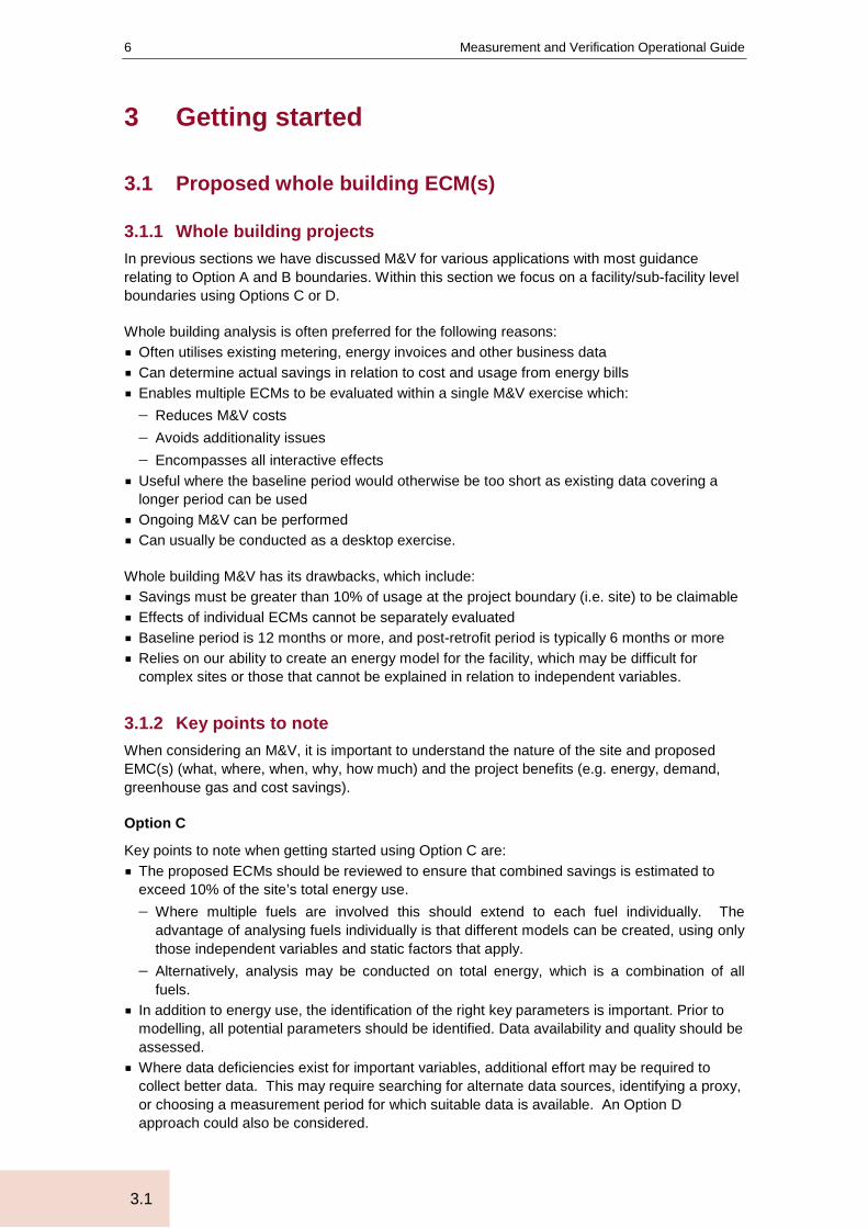
3.1.1 Whole building projects In previous sections we have discussed M&V for various applications with most guidance relating to Option A and B boundaries. Within this section we focus on a facility/sub-facility level boundaries using Options C or D.
Whole building analysis is often preferred for the following reasons: § Often utilises existing metering, energy invoices and other business data § Can determine actual savings in relation to cost and usage from energy bills § Enables multiple ECMs to be evaluated within a single M&V exercise which: − Reduces M&V costs − Avoids additionality issues − Encompasses all interactive effects § Useful where the baseline period would otherwise be too short as existing data covering a
longer period can be used § Ongoing M&V can be performed § Can usually be conducted as a desktop exercise.
Whole building M&V has its drawbacks, which include: § Savings must be greater than 10% of usage at the project boundary (i.e. site) to be claimable § Effects of individual ECMs cannot be separately evaluated § Baseline period is 12 months or more, and post-retrofit period is typically 6 months or more § Relies on our ability to create an energy model for the facility, which may be difficult for
complex sites or those that cannot be explained in relation to independent variables.
3.1.2 Key points to note When considering an M&V, it is important to understand the nature of the site and proposed EMC(s) (what, where, when, why, how much) and the project benefits (e.g. energy, demand, greenhouse gas and cost savings).
Option C
Key points to note when getting started using Option C are: § The proposed ECMs should be reviewed to ensure that combined savings is estimated to
exceed 10% of the site’s total energy use. − Where multiple fuels are involved this should extend to each fuel individually. The
advantage of analysing fuels individually is that different models can be created, using only those independent variables and static factors that apply.
− Alternatively, analysis may be conducted on total energy, which is a combination of all fuels.
§ In addition to energy use, the identification of the right key parameters is important. Prior to modelling, all potential parameters should be identified. Data availability and quality should be assessed. § Where data deficiencies exist for important variables, additional effort may be required to
collect better data. This may require searching for alternate data sources, identifying a proxy, or choosing a measurement period for which suitable data is available. An Option D approach could also be considered.

Getting started
7
3.1
§ The nature of the ECMs to be implemented is only somewhat important. It is a good idea to understand the type of ECM and the areas it may affect, however with a facility level boundary it will not alter the data that is collected. Consideration should be made if the ECM involves changes to independent variables to ensure that the developed model will provide a realistic adjusted baseline once the project is implemented. § Measurement periods are typically 12 months or more for baseline data and 6 months or
more for post-retrofit data. § Ongoing M&V may be considered, assuming that ongoing data for energy use, independent
variables and static factors can be collected and that the baseline energy model is still valid. § Using an ongoing approach, the effects of a staged implementation program can be
progressively reported. § Determine the desired level of uncertainty (precision + confidence). § Determine the required and desirable M&V outcomes. § Savings accuracy is dependent on the accuracy input data and the accuracy of the developed
model.
Option D
Key points to note when getting started using Option D are: § Computer simulation software is used to predict the facility energy use. This is applicable for
new buildings and for retrofits where baseline data cannot be obtained. § Energy use is predicted by inputting all key characteristics of the building, including: − Physical properties of building materials (walls, floors, roof, windows, partitions, doors,
insulation) − Site specific information, including location, reflectivity of external surfaces, wind
conditions, shading from external objects − Infiltration rates (how well the building is sealed) − Internal loads, including occupancy density, metabolic rate (activity levels and clothing) − Occupancy patterns (occupation levels at various times) − Equipment details (energy using equipment including size, power draw, equipment usage
patterns and control strategies, heat output) − Lighting details (types, numbers, locations of lights and/or lighting density, heat output,
operating schedules) − Air conditioning / refrigeration equipment (type and operation, electrical loads, coefficients
of performance, operating schedules and control strategies) − Data for independent variables and process loads (e.g. weather/temperature, wind, rainfall,
process equipment and corresponding heat loads, raw material inputs, and production outputs)
§ Determine the desired level of uncertainty (precision + confidence). § Determine the required and desirable M&V outcomes. § Accuracy is determined from the uncertainties associated with data collection, combined with
the calibration error between the developed model and the actual energy use data. § When the building is modelled, various scenarios are considered, known as ‘Off-Axis’ or ‘what
if’ scenarios. Examples include: − Part of building switches from 9am-5pm operation to 24/7. − Variable air volume dampers get stuck open − Tri-generation system has to be shut down. § Accurate computer modelling and calibration against actual usage are key challenges.
Simulation results must match for both usage and demand from monthly data. § Modelling incorporates 12 months of data, usually in hourly or half-hourly increments. § Ongoing M&V may be considered, assuming that ongoing data for energy use, independent
variables and static factors can be collected and that the baseline energy model is still valid.

Measurement and Verification Operational Guide
8
3.2
3.2 Decide approach for pursuing M&V Once the nature of the M&V project is scoped and the benefits assessed, the form of the M&V can be determined. Decide which M&V approach you wish to pursue: 1. Conduct project-level M&V 2. Conduct program-level M&V using a sample based approach incorporating project level
M&V supplemented with evaluation within the program ‘population’. 3. Adopt a non-M&V approach in which savings are estimated, or nothing is done.

M&V design and planning
9
4.1
4 M&V design and planning
4.1 M&V design
4.1.1 M&V Option Option C is the most common form of facility based analysis, which involves the development of an energy model from historical meter/billing data combined with data for independent variables across the site.
Option D is used where there is no baseline data. The site is modelled in detail, usually via specialised energy modelling software. The model is built from the ‘bottom up’, including a full asset list and equipment ratings, operating schedules, control strategies, and data for site-based independent variables.
Both options involve a long-term approach for conducting M&V.
4.1.2 Measurement boundary Either facility level boundary using Option C or Option D. Option D may also be used in conjunction with an ECM boundary. The energy system’s usage must be separated from the rest of the facility using a permanent meter
4.1.3 Key parameters For whole building M&V we need to consider the key parameters shown in the diagram and table below.
Non Routine Adjustments
Energy UsePerformance
Routine Adjustments
Equipment, Energy System, Functional
Area of Whole Facility
M&V OptionInteractive
Effects

Measurement and Verification Operational Guide
10
4.1
Table 2: key parameters to be considered when conducting M&V for whole building projects
Parameter Description
Energy use Energy use is typically obtained from the site’s incoming revenue meter or from energy invoices. Measurement periods may be short, such as 15/30 minute interval data for electricity or natural gas, through to monthly or quarterly invoices. Where billing periods are long, meters can be read periodically (e.g. weekly, monthly) to segment billing periods into shorter time intervals. Bulk fuels (e.g. diesel, petrol, LPG, coal, etc) are often stockpiled on site, which may lead to differences between the fuel’s purchase and subsequent use. It is important that data is captured for the time period (quantities and dates/times) when the fuel is used. This may require downstream metering (e.g. fuel pump readings taken when vehicles are filled, rather than relying on bulk fuel purchases which may be periodic or sporadic). Internal sub-metering can be used to describe a portion of a facility (e.g. buildings within a larger campus) or major energy systems.
Routine adjustments and performance outputs via independent variables
The identification of independent variables that affect a site is an important step for assessing sites using Options C or D. It is important to consider variables that may influence use across the measurement boundary, and these may include variables that are within the site’s control as well as those that occur naturally. Examples of independent variables include: § Weather – including ambient temperature, humidity, rainfall, wind
speed/direction § Operating hours – daily/weekly/seasonal operating schedules § Occupancy – staff, students, patients, shoppers, tenants, visitors, etc § System loads/ activity levels – heating/cooling requirements, temperature set
points, work required from equipment, etc § Input raw materials – temperatures, purity, density, moisture content, etc § Production types and amounts – product quantities, volumes, weight, etc Where a site engages in multiple activities, data for each may be required in order to effectively model site energy use. With all independent variables it is important that the range of possible values is known.
Non-routine adjustments via static factors
Given the long-term approach taken when using Option C and D, the effects of non-routine adjustments may become significant and require once off or permanent adjustments. The identification and collection of data relating to static factors may assist with identifying or adjusting outlying data points, or with making a permanent step change in modelling forecast figures. Typical static factors include material and permanent changes to independent variables listed above, as well as: § Change in product mix (e.g. plant stops making product A and start making
product B) § Equipment retrofits (either directly related to energy or not) § Production schedule/shift changes § Building changes (renovation, extension, facade changes, etc) § Extreme and infrequent weather events (flood, fire, cyclone, etc) § Effects of ECMs
4.1.4 Interactive effects Since total facility energy consumption is captured within the measurement boundary, interactive effects between energy systems will be accounted for.

M&V design and planning
11
4.2
4.1.5 Operating cycle When using Option C or D, the baseline period is 12 months or more, and post-retrofit period is typically 6 months or more
4.1.6 Additionality Since total facility energy consumption is captured within the measurement boundary, additionality will not be an issue for the M&V project.
4.2 Prepare M&V plan The next step of the M&V process is to prepare an M&V plan which is based on the M&V design and the time, resources and budget necessary to complete the M&V project.
Refer to the Planning Guide for further guidance on preparing an M&V plan.
The table below outlines issues commonly found when conducting M&V on whole building projects and provides suggested approaches for addressing them in you M&V plan and when executing the M&V project.
Table 3: Considerations, issues and suggested approach for whole building projects
Consideration Issue Suggested Approach
Modelling software and modelling/simulation skills
Insufficient skill or familiarity with complex modelling tools
Seek formal training on use of specific software packages. The software vendor is a useful place to start enquiries. OR Engage a suitably qualified professional to conduct the analysis
Difficult sites to model
Certain site types Consider variations to linear regression, including:
§ Multivariable regression
§ Non-linear curves
§ Stepped regression
§ Separate regression for each fuel type Consider alternatives to regression including bottom up energy use models using Option D.
Validating regression models
Understanding the process for validating regression models
Refer to the Process Guide for further information.
Measurement and Verification Operational Guide
12
5.1
5 Data collection, modelling and analysis
5.1 Measure baseline data
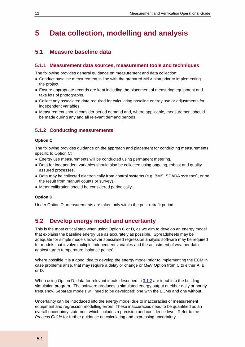
5.1.1 Measurement data sources, measurement tools and techniques The following provides general guidance on measurement and data collection: § Conduct baseline measurement in line with the prepared M&V plan prior to implementing
the project. § Ensure appropriate records are kept including the placement of measuring equipment and
take lots of photographs. § Collect any associated data required for calculating baseline energy use or adjustments for
independent variables. § Measurement should consider period demand and, where applicable, measurement should
be made during any and all relevant demand periods.
5.1.2 Conducting measurements
Option C
The following provides guidance on the approach and placement for conducting measurements specific to Option C: § Energy use measurements will be conducted using permanent metering. § Data for independent variables should also be collected using ongoing, robust and quality
assured processes. § Data may be collected electronically from control systems (e.g. BMS, SCADA systems), or be
the result from manual counts or surveys. § Meter calibration should be considered periodically.
Option D
Under Option D, measurements are taken only within the post-retrofit period.
5.2 Develop energy model and uncertainty This is the most critical step when using Option C or D, as we aim to develop an energy model that explains the baseline energy use as accurately as possible. Spreadsheets may be adequate for simple models however specialised regression analysis software may be required for models that involve multiple independent variables and the adjustment of weather data against target temperature ‘balance points’.
Where possible it is a good idea to develop the energy model prior to implementing the ECM in case problems arise, that may require a delay or change or M&V Option from C to either A, B or D.
When using Option D, data for relevant inputs described in 3.1.2 are input into the building simulation program. The software produces a simulated energy output at either daily or hourly frequency. Separate models will need to be developed; one with the ECMs and one without.
Uncertainty can be introduced into the energy model due to inaccuracies of measurement equipment and regression modelling errors. These inaccuracies need to be quantified as an overall uncertainty statement which includes a precision and confidence level. Refer to the Process Guide for further guidance on calculating and expressing uncertainty.

Data collection, modelling and analysis
13
5.3
5.3 Implement ECM(s) Implement the ECM. Under Option C, this may have already occurred, which shouldn’t be an issue if a successful energy model has been determined. Ensure that appropriate commissioning has been conducted to confirm that the ECMs are operating as expected.
Under Option D, the new building is constructed or the ECM is implemented.
5.4 Measure post retrofit data Option C
Conduct post-retrofit measurement in line with the prepared M&V plan using the same techniques as for the baseline (section 5.1).
Collect any associated data required for calculating post-retrofit energy use or adjustments based on independent variables (e.g. monthly heating and/or cooling degree days). Confirm data integrity and completeness.
Option D
Post-retrofit data for energy use, independent variables and static factors is collected, allowing a suitable time to commission the building or ‘bed in’ a new ECM. § Measurements are taken only within the post-retrofit period. § Energy use measurements will be conducted using permanent metering. § Data for independent variables should also be collected using ongoing, robust and quality
assured processes. § Data may be collected electronically from control systems (e.g. BMS, SCADA systems), or be
the result from manual counts or surveys. Meter calibration should be considered periodically.
5.5 Savings analysis and uncertainty
5.5.1 Savings equations
Option C
The energy model previously developed is now used to forecast across the post-retrofit the business as usual consumption which would have occurred without the ECM. This is achieved by applying the various data inputs specified by the model for independent variables and static factors.
Savings are then calculated by subtracting the business as usual forecast from the actual savings from the metered energy use. From an uncertainty point of view, billed energy data is considered 100% accurate. Other uncertainties will be dependent on the modelling uncertainty, plus those from data collection.
The general equation for energy savings is:
Energy Savings = (Baseline Energy – Post-Retrofit Energy) ± Adjustments

Measurement and Verification Operational Guide
14
5.5
Option D
Calibrate the building simulation against post-retrofit energy use and conditions to calculate savings: § Both developed simulation models (simulation models with and without ECMs) are re-
calibrated using data from the post-retrofit period for all key independent variables. The installed equipment and controls, internal heat loads and other characteristics are confirmed and adjusted. § Changes are applied to both models as required, based on the concept of calibrating the
model that contains the ECMs (i.e. ‘as built’ model) so that it accurately reflects the metered energy use from the measurement boundary. § It should confirm that it appropriately describes both the energy use and demand profile from
monthly data. 12 months of post-retrofit data is used to calibrate the model. § Actual weather data is also used. § Once off or short term measurement of individual equipment may assist with appropriately
calibrating the model for complex systems. § The calibration error is determined at a monthly level using the ‘as-built’ model and the actual
energy data. Calibration errors are applied to the baseline model in order to incorporate uncertainty within savings. § Savings are calculated in one of two ways: − Actual savings = Actual energy use – calibrated baseline model, OR − Normalised savings = calibrated as-built model – calibrated baseline model § Actual savings are determined for the post-retrofit period, by applying the appropriate data to
the baseline model. § Normalised savings can be determined using any set of data for independent variables (e.g.
10 year average weather patterns), once the models are calibrated. The data is applied to both models.
5.5.2 Extrapolation Extrapolate the calculated savings for the measured period as required.
5.5.3 Uncertainty Estimate the savings uncertainty, based on the measurement approach, placement, impact of variables, length of measurement and equipment used. Refer to the Process Guide for further guidance on calculating and expressing uncertainty.

Finish
15
6.1
6 Finish
6.1 Reporting Prepare an outcomes report summarising the M&V exercise. Ensure any extrapolated savings are referred to as estimates, as the ‘actual’ savings only apply to the measurement period. Energy uncertainty is expressed with the overall precision and confidence level.
6.2 Project close and savings persistence Under Option C, ongoing M&V can be conducted regularly as required by collecting independent variables and inserting them into the energy model. Typically under Option D, the first year of data forms the baseline of an ongoing Option C M&V approach.
Measurement and Verification Operational Guide
16
7.1
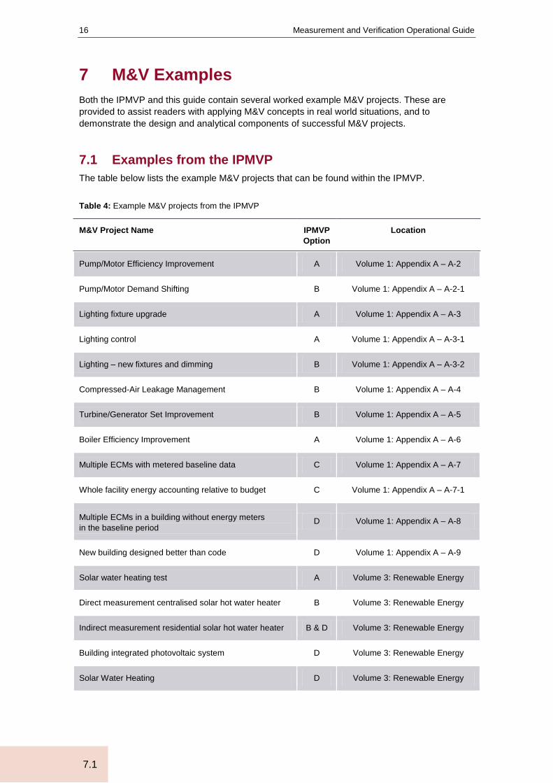
7 M&V Examples Both the IPMVP and this guide contain several worked example M&V projects. These are provided to assist readers with applying M&V concepts in real world situations, and to demonstrate the design and analytical components of successful M&V projects.
7.1 Examples from the IPMVP The table below lists the example M&V projects that can be found within the IPMVP.
Table 4: Example M&V projects from the IPMVP
M&V Project Name IPMVP Option
Location
Pump/Motor Efficiency Improvement A Volume 1: Appendix A – A-2
Pump/Motor Demand Shifting B Volume 1: Appendix A – A-2-1
Lighting fixture upgrade A Volume 1: Appendix A – A-3
Lighting control A Volume 1: Appendix A – A-3-1
Lighting – new fixtures and dimming B Volume 1: Appendix A – A-3-2
Compressed-Air Leakage Management B Volume 1: Appendix A – A-4
Turbine/Generator Set Improvement B Volume 1: Appendix A – A-5
Boiler Efficiency Improvement A Volume 1: Appendix A – A-6
Multiple ECMs with metered baseline data C Volume 1: Appendix A – A-7
Whole facility energy accounting relative to budget C Volume 1: Appendix A – A-7-1
Multiple ECMs in a building without energy meters in the baseline period
D Volume 1: Appendix A – A-8
New building designed better than code D Volume 1: Appendix A – A-9
Solar water heating test A Volume 3: Renewable Energy
Direct measurement centralised solar hot water heater B Volume 3: Renewable Energy
Indirect measurement residential solar hot water heater B & D Volume 3: Renewable Energy
Building integrated photovoltaic system D Volume 3: Renewable Energy
Solar Water Heating D Volume 3: Renewable Energy

M&V Examples
17
7.2
7.2 Examples from this guide The table below lists the example M&V projects that can be found within this guide.
Table 5: Example M&V projects from the M&V Operational Guide
M&V Project Name IPMVP Option Location
M&V design examples A, B, C, D Process: Appendix A
Demand and cost avoidance calculation example n/a Process: Appendix A
Regression modelling and validity testing n/a Process: Appendix E
Lighting fixture replacement within an office tenancy A Applications: Lighting – Scenario A
Lighting fixture and control upgrade at a function centre A Applications: Lighting – Scenario B
Lighting fixture retrofit incorporating daylight control B Applications: Lighting – Scenario C
Pump retrofit and motor replacement A Applications: Motors, Pumps and Fans –
Scenario A
Car park ventilation involving CO monitoring and variable speed drive on fans
B Applications: Motors, Pumps and Fans – Scenario B
Replacement an inefficient gas boiler with a high efficiency one C Applications: Heating, Ventilation and
Cooling – Scenario A
Upgrade freezer controls within a food processing plant B Applications: Commercial and Industrial
Refrigeration – Scenario A
Compressed air leak detection within a manufacturing site using sampling analysis
B Applications: Boilers, Steam and Compressed Air – Scenario A
Steam system leak detection within a food processing site using regression analysis
B Applications: Boilers, Steam and Compressed Air – Scenario B
Multiple ECMs involving compressed air and steam system optimisation, combined with lighting controls at a cannery
C Applications: Whole Buildings – Scenario A
Commercial building air conditioning central plant upgrade C Applications: Whole Buildings –
Scenario B
Evaluate performance efficiency of a newly installed cogeneration unit a a school
D Applications: Renewables and Cogeneration – Scenario A
Installation of a cogeneration plant at a hospital C Applications: Renewables and
Cogeneration – Scenario B
Use of solar hot water system on a housing estate B Applications: Renewables and
Cogeneration – Scenario C

Measurement and Verification Operation Guide
18
Appendix A
Appendix A: Example scenario A – food processing plant The scenario below provides details of how Option C is used to measure and verify the savings from multiple ECMs across a manufacturing plant.
A food processing plant in a regional town prepares and packages a range of tinned and snap frozen vegetable products grown in the local area. The plant operates year-round, however activity in a given month is seasonal based on the produce and consumer spending patterns.
The plant consists of several production lines, some of which serve multiple products throughout the year. Broad beans, which are the plant’s most popular product is highly seasonal and is only produced for 5 months of the year.
The basic process involves food preparation (skinning, dehusking, etc), cooking, and either snap freezing and packaging, or canning. A centralised set of boilers provide hot water and steam for cooking and sterilisation, whilst a set of air compressors provide compressed air for operating much of the machinery.
The site is a significant energy user and receives monthly invoices for electricity and natural gas. At present there is no sub-metering of energy use across the site.
Following an energy audit, the Site Manager has gained approval to proceed with implementing several ECMs across the site. At first the low cost measures are to be implemented and once savings can be verified, capital will be available for more significant upgrades.
The identified ECMs are mostly small to medium and include: 1. Adding a heat exchanger to capture waste heat from the air compressor system to
pre-heat boiler feedwater. 2. Reducing compressed air and steam delivery pressures 3. Introducing occupancy based lighting controls for seldom used areas
When combined together, the Site Manager estimates that the above ECMs will reduce site energy use by around 15%. Each ECM relates to a different energy system, and there is the potential to assess each individually.
Monthly energy use is highly variable, which the Site Manager believes is due to changes in product output, however she cannot be sure. The Site Manager is only interested in determining combined savings, and does not have the funds available to invest in temporary metering.
More importantly, the Site Manager seeks to develop an approach for conducting M&V that will apply into the future as more ECMs are implemented.
For these reasons, an Option C approach is to be used to verify savings. Management are interested in savings to a confidence of 90%.

Appendix A: Example scenario A – food processing plant
19
Appendix A
Getting started
Budget The potential savings (15% of site usage) from these projects are significant, however the site is has complex, interlinked manufacturing processes. Due to the difficulty of defining appropriate project measurement boundaries, combined with the fact that the Site Manager does not have funds for temporary metering, an Option C approach has been adopted which simply involves desktop analysis using existing data. It is anticipated that the analysis can be conducted and savings calculated within 12 hours. A nominal budget of $2,500 of time has been set aside.
Measurement boundary The measurement boundary is the combination of electrical and natural gas supplies that supply the facility. Both fuels will be affected by the proposed ECMs. Although the Site Manager is only interested in overall savings, separate analysis will be conducted for electricity and natural gas in order to calculate cost savings.
Identification of key parameters After working at the site for a number of years in various roles, the Site Manager has developed her opinion regarding the variables that may affect energy use. She hasn’t conducted detailed analysis before to determine these, and so she plans on collecting data for the following variables and attempting various models to find the best combinations of data. The variables to be investigated include:
Variable Data source
Metered electricity and natural gas use Monthly electricity invoices
Ambient air temperature (heating and cooling degree days)
Daily figures for maximum and minimum air temperatures from the Bureau of Meteorology
Production figures for various product lines, divided into: § Canned Mixed Vegetables § Broad beans § Peas § Other production (combined)
Monthly site reports which include data compiled from shift-based production outputs
The plant operates continuously, and so operating hours will not be considered. However some products are highly seasonal, which will be reflected in the monthly production volumes.
Timing Baseline data is available for the last 3 years. The ECMs are due to be implemented during September 2010, and so the period just prior has been chosen. The baseline period will consist of the 12 months between September 2009 and August 2010.
Interactive effects There are no interactive effects due to the choice of a facility based measurement boundary.

Measurement and Verification Operational Guide
20
Appendix A
Summary of M&V plan The key elements of the project’s M&V plan in summary are:
Item Plan
Project Summary Implementation of the following ECMs on central service equipment: § waste heat capture from the air compressor system to pre-heat boiler
feedwater § pressure reduction strategy for compressed air and steam systems § occupancy based control of lighting in seldom used areas
Required Outcome To confirm savings in excess of 15% with a 90% confidence level in order to convince management to invest in more capital intensive energy efficiency projects.
Budget $2,500 (1 day of desktop analysis)
M&V Option C – Whole Facility
Measurement Boundary Total incoming electrical and natural gas supplies being fed to the BeanCo Central West Processing Plant, located in 23 Rabie Road, Parkes, NSW.
Key Measurement Parameters
Data for the following key parameters will be collected and modelled in order to determine the most relevant factors affecting energy use: § Metered electricity and natural gas use § Ambient temperature (in the form of heating/cooling degree days) § Monthly production figures for processed goods
− Canned mixed vegetables − Broad beans − Peas − Other food products
Other Parameters to consider
None identified
Potential interactive effects None identified
Approach for conducting measurement and collecting data
Energy use data will be collected directly from energy invoices. Ambient temperature data will be sourced for the nearest weather station from the Bureau of Meteorology. Production data will be obtained from monthly reports, which are compiled from daily shift data.
Measurement equipment required
Existing revenue meter and energy invoice data
Measurement period 12 month base year period, 1 month project implementation, and 6+ month post-retrofit measurement.
Appendix A: Example scenario A – food processing plant
21
Appendix A
Item Plan
Approach for calculating results
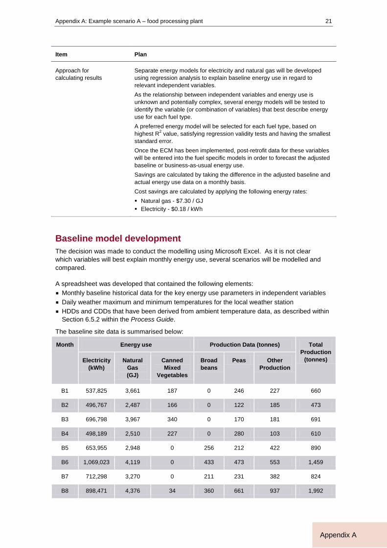
Separate energy models for electricity and natural gas will be developed using regression analysis to explain baseline energy use in regard to relevant independent variables. As the relationship between independent variables and energy use is unknown and potentially complex, several energy models will be tested to identify the variable (or combination of variables) that best describe energy use for each fuel type. A preferred energy model will be selected for each fuel type, based on highest R2 value, satisfying regression validity tests and having the smallest standard error. Once the ECM has been implemented, post-retrofit data for these variables will be entered into the fuel specific models in order to forecast the adjusted baseline or business-as-usual energy use. Savings are calculated by taking the difference in the adjusted baseline and actual energy use data on a monthly basis. Cost savings are calculated by applying the following energy rates: § Natural gas - $7.30 / GJ § Electricity - $0.18 / kWh
Baseline model development The decision was made to conduct the modelling using Microsoft Excel. As it is not clear which variables will best explain monthly energy use, several scenarios will be modelled and compared.
A spreadsheet was developed that contained the following elements: § Monthly baseline historical data for the key energy use parameters in independent variables § Daily weather maximum and minimum temperatures for the local weather station § HDDs and CDDs that have been derived from ambient temperature data, as described within
Section 6.5.2 within the Process Guide.
The baseline site data is summarised below:
Month Energy use Production Data (tonnes) Total Production
(tonnes) Electricity (kWh)
Natural Gas (GJ)
Canned Mixed
Vegetables
Broad beans
Peas Other Production
B1 537,825 3,661 187 0 246 227 660
B2 496,767 2,487 166 0 122 185 473
B3 696,798 3,967 340 0 170 181 691
B4 498,189 2,510 227 0 280 103 610
B5 653,955 2,948 0 256 212 422 890
B6 1,069,023 4,119 0 433 473 553 1,459
B7 712,298 3,270 0 211 231 382 824
B8 898,471 4,376 34 360 661 937 1,992

Measurement and Verification Operational Guide
22
Appendix A
Month Energy use Production Data (tonnes) Total Production
(tonnes) Electricity (kWh)
Natural Gas (GJ)
Canned Mixed
Vegetables
Broad beans
Peas Other Production
B9 882,253 5,523 34 280 25 685 1,024
B10 466,539 3,563 14 0 211 342 567
B11 451,487 4,072 18 0 326 296 640
B12 488,450 2,985 20 0 299 242 561
In addition to the data above, weather data was collected from the Bureau of Meteorology for the nearest weather station. From the average daily temperatures, values for Heating Degree Days (HDDs) and Cooling Degree Days (CDDs) were computed.
Initial values for HDD and CDD balance points were chosen, and were added into the analysis spreadsheet as reference values in linked cells. The balance points were adjusted as part of tuning various energy models so that the R2 value was maximised for each energy model.
The LINEST() function is used to conduct multivariable linear regression on a dataset to produce a function describing y in terms of x1 to n in the form:
y = b + m1x1 + m2x2 + ...+ mnxn
where:
y = energy use
b = baseload energy use (without influence of any variables) – also known as y-intercept
x1 to n = data for independent variables 1 to n
m1 to n = coefficients determined by the function that correspond to each x variable
It accepts an array of y-values (i.e. energy use) and corresponding arrays of x-values (data for independent variables) and produces various outputs as shown below: § Coefficients and standard errors for the baseload energy use (b) and each independent
variable (m1 to n) § Coefficient of determination (R2), and Adjusted R2 which describe the ‘appropriateness of fit’
for the regression model § Standard error for y
Developing the energy model for electricity Seven different regression models were calculated, each incorporating a different combination of parameters as shown in the table below.

Appendix A: Example scenario A – food processing plant
23
Appendix A
Scenario Electricity (kWh)
Production(tonnes) Total Production
(tonnes)
Ambient temperature
Canned Mixed
Vegetables
Broad Beans
Peas Other HDDs CDDs
1 Yes - - - - Yes - -
2 Yes - - - - Yes Yes -
3 Yes - - - - Yes - Yes
4 Yes Yes Yes - - - Yes Yes
5 Yes Yes Yes - - - - -
6 Yes Yes Yes - - - Yes -
7 Yes Yes Yes Yes - - Yes -
The combinations above were selected as the analysis proceeded. As each model was developed, the t-stats for each coefficient were examined to see which variables were providing a strong correlation. Any coefficient with a t-stat value less than 2 was further examined in subsequent models. In addition, changes in R2 provided a guide as to how each model reacted to inclusion of new variables, based on a base model involving total production.
Refer to Help within Microsoft Excel for assistance with using the LINEST() function. An example of the output using the input data above for Scenario 6 is shown below:
The output above equates to the following:
Energy use = 334,632.808
+ 588.668 x (HDD)
+ 915.970 x (Canned Mixed Vegetables (tonnes))
+ 1,549.486 x (Broad Beans (tonnes))
The R2 value is 0.950 and the standard error is 55,369.565
Each model was generated in turn using the LINEST() function.
coefficients
standard errors for coefficients standard error for y R2
t-stats – calculated separately

Measurement and Verification Operational Guide
24
Appendix A
Validating the regression outputs As described in Section 6.5.1, each model must be validated to confirm that it can be used. This involves equating some additional attributes and confirming their validity. The attributes to be reviewed are:
Attribute Description and Validity Test
R2 Must be 0.75 or higher. Output from LINEST() function
Adjusted R2
To be evaluated when multiple independent variables are used. Values should be 0.75 or higher. Calculated as follows:
𝐴𝑑𝑗𝑢𝑠𝑡𝑒𝑑 𝑅2 = 1 − (1 − 𝑅2) ×(𝑛 − 1)
(𝑛 − 𝑘 − 1)
Where: R2 = the value calculated from LINEST() n = number of data points in sample size k = number of coefficients within the regression model
t-statistic for each coefficient
Determine the validity of each x coefficient. Values must be greater than 2. Calculated as follows: Each ‘t-stat’ is calculated as follows:
𝑡𝑋𝑛 =𝑐𝑜𝑒𝑓𝑓𝑖𝑐𝑖𝑒𝑛𝑡𝑋𝑛
𝑠𝑡𝑎𝑛𝑑𝑎𝑟𝑑 𝑒𝑟𝑟𝑜𝑟𝑋𝑛
Absolute mean bias (MBE)
Determines the overall bias in the regression estimate. MBE values should be < 0.005%. Calculated as follows:
𝑀𝐵𝐸 =∑(𝑚𝑜𝑑𝑒𝑙𝑙𝑒𝑑𝑛 − 𝑎𝑐𝑡𝑢𝑎𝑙𝑛)
𝑛
Where: n = the number of samples modelledn = predicted value for sample item n actualn = actual value for sample item n
Monthly Mean Error CV(RMSE) Related to the standard error of the model. CV(RMSE) values should be < 0.25. Calculated as follows:
𝐶𝑉(𝑅𝑀𝑆𝐸) =𝑠𝑡𝑎𝑛𝑑𝑎𝑟𝑑 𝑒𝑟𝑟𝑜𝑟 𝑓𝑜𝑟 𝑦𝑎𝑣𝑒𝑟𝑎𝑔𝑒(𝑎𝑐𝑡𝑢𝑎𝑙 𝑣𝑎𝑙𝑢𝑒𝑠)

Appendix A: Example scenario A – food processing plant
25
Appendix A
In our example above:
𝐴𝑑𝑗𝑢𝑠𝑡𝑒𝑑 𝑅2 = 1 − (1 − 0.950) ×(12 − 1)
(12 − 3 − 1)= 0.931
For our three coefficients in the example above:
𝑡𝑐𝑎𝑛𝑛𝑒𝑑 𝑚𝑖𝑥𝑒𝑑 𝑣𝑒𝑔𝑒𝑡𝑎𝑏𝑙𝑒𝑠 =915.970224.833
= 4.07
𝑡𝑏𝑟𝑜𝑎𝑑 𝑏𝑒𝑎𝑛𝑠 =1,549.486154.349
= 10.04
𝑡𝐻𝐷𝐷𝑠 =588.668287.335
= 2.05
MBE is calculated by first determining the modelled energy values by using the data for independent variables. Modelled values are then subtracted from actual values to calculate the difference for each measurement. These residuals are summed and divided by the number of data points to determine the MBE, as follows:
Month Actual energy Example Scenario 6 modelled energy
Residual (modelled – actual)
B1 537,825 553,614 15,789
B2 496,767 505,050 8,283
B3 696,798 650,419 -46,379
B4 498,189 544,030 45,841
B5 653,955 731,301 77,346
B6 1,069,023 1,005,560 -63,463
B7 712,298 661,574 -50,724
B8 898,471 942,046 43,575
B9 882,253 891,876 9,623
B10 466,539 452,269 -14,270
B11 451,487 478,067 26,580
B12 488,450 436,249 -52,201
Sum -5.82 x 10—10
Average 654,337.92
And, MBE is calculated as follows:
𝑀𝐵𝐸 =−5.82 × 10⁻¹⁰
12= −4.85 × 10⁻¹¹
CV(RMSE) is calculated for the example above as follows:
𝐶𝑉(𝑅𝑀𝑆𝐸) =53,361.49
654,337.92= 0.0816

Measurement and Verification Operational Guide
26
Appendix A
Validity tests for each of the seven models were conducted. The results are shown in the table below. Conditional formatting is used to highlight test results. Each value is coloured green if it passes the validity test and red if it fails.
Scenarios 5 and 6 pass all the validity tests. Scenario 6 was selected from the table above as the preferred scenario as it had the highest R2 and Adjusted R2 values and the lowest standard error.
Summarising the electricity model The output from the LINEST() function for Scenario 6 is shown below.
From the above the energy model describes monthly energy use as:
𝐸𝑙𝑒𝑐𝑡𝑟𝑖𝑐𝑖𝑡𝑦 𝑢𝑠𝑒(𝑘𝑊ℎ)= 334,633 + (588.67 × 𝐻𝐷𝐷𝑠) + (915.97 × 𝐶𝑎𝑛𝑛𝑒𝑑 𝑀𝑖𝑥𝑒𝑑 𝑉𝑒𝑔𝑒𝑡𝑎𝑏𝑙𝑒𝑠)+ (1,549.49 × 𝐵𝑟𝑜𝑎𝑑 𝐵𝑒𝑎𝑛𝑠)
And the standard error is ± 53,361.49 kWh
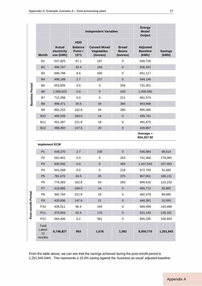
Calculating electricity savings The ECM was implemented in September 2010. Following a number of months, the savings were calculated for the ECM by forecasting the adjusted baseline by applying post-retrofit data to the baseline energy model. This is shown in the table below.
Appendix A: Example scenario A – food processing plant
27
Appendix A
Independent Variables
Energy Model Output
Month
Actual electricity use (kWh)
HDD Balance Point =
13°C
Canned Mixed Vegetables
(tonnes)
Broad Beans
(tonnes)
Adjusted Baseline
(kWh) Savings (kWh)
Bas
elin
e Pe
riod
B1 537,825 87.1 187 0 556,726
B2 496,767 33.4 166 0 506,331
B3 696,798 8.6 340 0 651,117
B4 498,189 2.7 227 0 544,146
B5 653,955 0.0 0 256 731,301
B6 1,069,023 0.0 0 433 1,005,560
B7 712,298 0.0 0 211 661,574
B8 898,471 34.5 34 360 943,908
B9 882,253 162.8 34 280 895,485
B10 466,539 184.0 14 0 455,761
B11 451,487 221.8 18 0 481,675
B12 488,450 147.6 20 0 439,857
Average = 654,337.92
Implement ECM
Post
-ret
rofit
Per
iod
P1 448,370 2.7 230 0 546,984 98,614
P2 562,401 0.0 0 263 741,466 179,065
P3 930,050 0.0 0 454 1,037,543 107,493
P4 641,068 0.0 0 218 672,750 31,682
P5 781,670 34.5 35 375 967,801 186,131
P6 776,383 162.8 34 283 899,616 123,233
P7 419,885 184.0 14 0 455,772 35,887
P8 392,794 221.8 19 0 482,479 89,685
P9 429,836 147.6 21 0 440,391 10,555
P10 426,011 96.4 194 0 569,499 143,488
P11 375,953 52.4 170 0 521,134 145,181
P12 564,406 0.2 361 0 665,335 100,929
Total Latest
12 months
6,748,827 903 1,078 1,592 8,000,770 1,251,943
From the table above, we can see that the savings achieved during the post-retrofit period is 1,251,943 kWh. This represents a 15.6% saving against the ‘business as usual’ adjusted baseline.

Measurement and Verification Operational Guide
28
Appendix A
Cost savings are calculated by applying the agreed cost rate to the electricity savings figure as follows:
𝐶𝑜𝑠𝑡 𝑠𝑎𝑣𝑖𝑛𝑔𝑠 ($) = 𝑒𝑛𝑒𝑟𝑔𝑦 𝑠𝑎𝑣𝑖𝑛𝑔𝑠 (𝑘𝑊ℎ) × 𝑒𝑛𝑒𝑟𝑔𝑦𝑐𝑜𝑠𝑡 𝑟𝑎𝑡𝑒 ($
𝑘𝑊ℎ)
𝐶𝑜𝑠𝑡 𝑠𝑎𝑣𝑖𝑛𝑔𝑠 ($) = 1,251,943𝑘𝑊ℎ ×$0.18𝑘𝑊ℎ
𝐶𝑜𝑠𝑡 𝑠𝑎𝑣𝑖𝑛𝑔𝑠 ($) = $225,349.74
The actual energy use is plotted against the baseline and adjusted baseline. The energy savings are shown in green.
Uncertainty analysis As shown earlier, the standard error (SE) of the baseline energy model is:
𝑠𝑡𝑎𝑛𝑑𝑎𝑟𝑑 𝑒𝑟𝑟𝑜𝑟(𝑆𝐸) = 53,361.49 𝑘𝑊ℎ
Using the standard error we can calculate the absolute precision (AP) by applying the t-statistic for our chosen sample size (where DF = 12 data points – 3 variables -1 = 8) and required confidence (90%). Refer to Table 27 within Appendix G of the Process Guide for the list of t-statistics.
Absolute precision is calculated as follows:
𝐴𝑏𝑠𝑜𝑙𝑢𝑡𝑒 𝑝𝑟𝑒𝑐𝑖𝑠𝑖𝑜𝑛 (𝐴𝑃) = 𝑡 × 𝑆𝐸
𝐴𝑏𝑠𝑜𝑙𝑢𝑡𝑒 𝑝𝑟𝑒𝑐𝑖𝑠𝑖𝑜𝑛 (𝐴𝑃) = 1.86 × 53,361.49 = 99,252.37 𝑘𝑊ℎ
And the relative precision (RP) is calculated by dividing the absolute precision by the average predicted energy use as follows:

Appendix A: Example scenario A – food processing plant
29
Appendix A
𝑟𝑒𝑙𝑎𝑡𝑖𝑣𝑒 𝑝𝑟𝑒𝑐𝑖𝑠𝑖𝑜𝑛 (𝑅𝑃) =𝐴𝑃
𝑎𝑣𝑒𝑟𝑎𝑔𝑒 𝑚𝑜𝑛𝑡ℎ𝑙𝑦 𝑚𝑜𝑑𝑒𝑙𝑙𝑒𝑑 𝑢𝑠𝑎𝑔𝑒
𝑟𝑒𝑙𝑎𝑡𝑖𝑣𝑒 𝑝𝑟𝑒𝑐𝑖𝑠𝑖𝑜𝑛 (𝑅𝑃) =99,252.37
654,337.92= ±15.2%
The uncertainty of the savings is calculated as follows:
𝑆𝐸(𝑚𝑜𝑛𝑡ℎ𝑙𝑦 𝑠𝑎𝑣𝑖𝑛𝑔𝑠) = �𝑆𝐸(𝑎𝑑𝑗𝑢𝑠𝑡𝑒𝑑 𝑏𝑎𝑠𝑒𝑙𝑖𝑛𝑒)2 + 𝑆𝐸(𝑝𝑜𝑠𝑡 𝑟𝑒𝑡𝑟𝑜𝑓𝑖𝑡)2
= �53,361.492 + 02 = 53,361.49 𝑘𝑊ℎ
Note that the post retrofit standard error is zero since we are using billing data as our source which is deemed to be 100% accurate.
Assuming that the standard error of each month’s savings will be the same, the standard error for the annual savings is:
𝑆𝐸(𝑎𝑛𝑛𝑢𝑎𝑙 𝑠𝑎𝑣𝑖𝑛𝑔𝑠) = �12 × 53,361.492 = 184,849.62 𝑘𝑊ℎ
Using a t-statistic of 1.80 (12 measurement points with 90% confidence, DF = 11), the range of possible annual savings will be:
𝑅𝑎𝑛𝑔𝑒 𝑜𝑓 𝑆𝑎𝑣𝑖𝑛𝑔𝑠 (𝑘𝑊ℎ) = 1,251,943 ± 1.80 × 184,849.62𝑘𝑊ℎ
= 1,251,943 ± 332,729 𝑘𝑊ℎ
The relative precision of the annual savings reported is thus ±26.6% (184,850 / 1,251,943)
Developing the energy model for natural gas A similar process was applied to the natural gas. As before seven different regression models were calculated, each incorporating a different combination of parameters as shown in the table below.
Production (tonnes)
Total Production
(tonnes)
Ambient temperature
Scenario Natural
Gas (GJ)
Canned Mixed
Vegetables Broad Beans Peas Other HDDs CDDs
1 Yes - - - - Yes - - 2 Yes - - - - Yes Yes - 3 Yes Yes Yes - - - - - 4 Yes Yes - - - - Yes - 5 Yes Yes - - Yes - Yes - 6 Yes Yes Yes - - - Yes - 7 Yes Yes Yes Yes - - Yes -
Again as before, validity tests for each of the seven models were conducted. The results are shown in the table below. Conditional formatting is used to highlight test results. Each value is coloured green if it passes the validity test and red if it fails.
Measurement and Verification Operational Guide
30
Appendix A
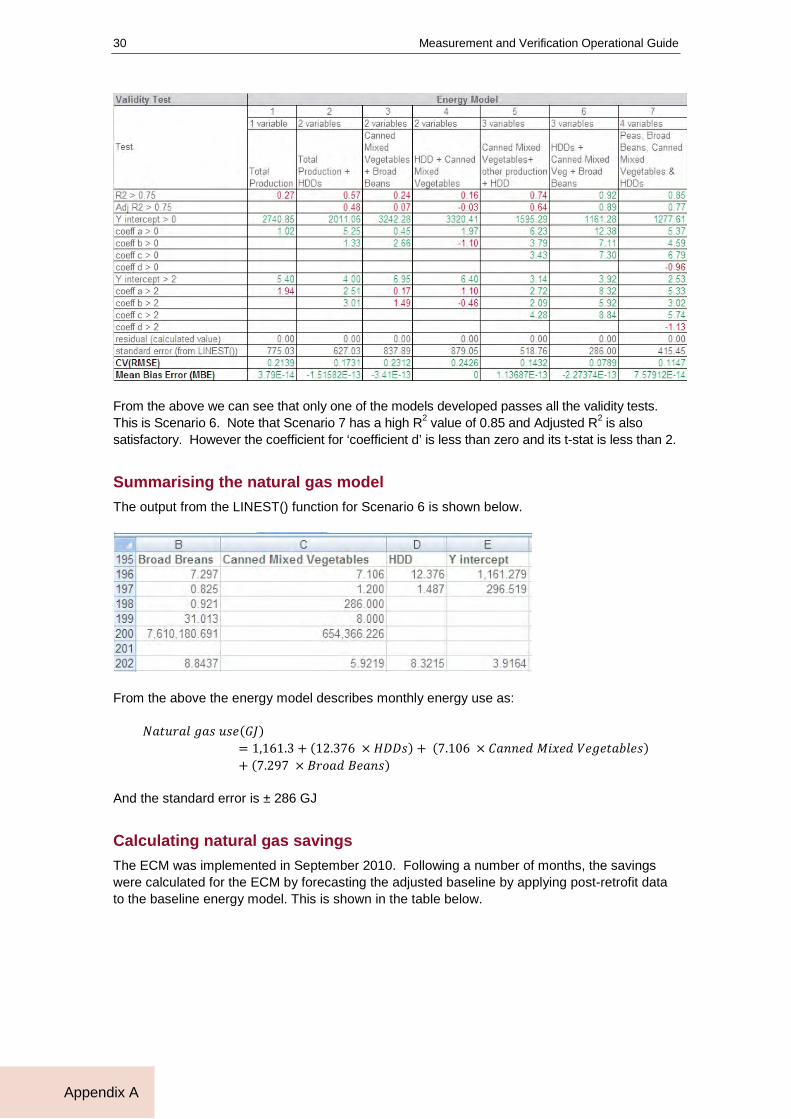
From the above we can see that only one of the models developed passes all the validity tests. This is Scenario 6. Note that Scenario 7 has a high R2 value of 0.85 and Adjusted R2 is also satisfactory. However the coefficient for ‘coefficient d’ is less than zero and its t-stat is less than 2.
Summarising the natural gas model The output from the LINEST() function for Scenario 6 is shown below.
From the above the energy model describes monthly energy use as:
𝑁𝑎𝑡𝑢𝑟𝑎𝑙 𝑔𝑎𝑠 𝑢𝑠𝑒(𝐺𝐽)= 1,161.3 + (12.376 × 𝐻𝐷𝐷𝑠) + (7.106 × 𝐶𝑎𝑛𝑛𝑒𝑑 𝑀𝑖𝑥𝑒𝑑 𝑉𝑒𝑔𝑒𝑡𝑎𝑏𝑙𝑒𝑠)+ (7.297 × 𝐵𝑟𝑜𝑎𝑑 𝐵𝑒𝑎𝑛𝑠)
And the standard error is ± 286 GJ
Calculating natural gas savings The ECM was implemented in September 2010. Following a number of months, the savings were calculated for the ECM by forecasting the adjusted baseline by applying post-retrofit data to the baseline energy model. This is shown in the table below.

Appendix A: Example scenario A – food processing plant
31
Appendix A
Independent Variables Energy Model Output
Month
Actual natural gas
use (GJ)
HDD Balance Point = 13.2°C
Canned Mixed
Vegetables (tonnes)
Broad Beans
(tonnes) Adjusted
Baseline (GJ) Savings
(GJ)
Bas
elin
e Pe
riod
B1 3,661 87.1 187 0 3,564
B2 2,487 33.4 166 0 2,754
B3 3,967 8.6 340 0 3,684
B4 2,510 2.7 227 0 2,808
B5 2,948 0.0 0 256 3,029
B6 4,119 0.0 0 433 4,321
B7 3,270 0.0 0 211 2,701
B8 4,376 34.5 34 360 4,457
B9 5,523 162.8 34 280 5,461
B10 3,563 184.0 14 0 3,538
B11 4,072 221.8 18 0 4,034
B12 2,985 147.6 0 0 2,988
Average = 3,612
Implement ECM
Post
-ret
rofit
Per
iod
P1 2,385 2.7 230 0 2,830 445
P2 2,801 0.0 0 263 3,077 276
P3 3,736 0.0 0 454 4,471 735
P4 2,786 0.0 0 218 2,754 -32
P5 3,926 34.5 35 375 4,572 646
P6 3,977 162.8 34 283 5,481 1,504
P7 2,779 184.0 14 0 3,538 759
P8 2,973 221.8 19 0 4,040 1,067
P9 2,358 147.6 0 0 2,988 630
P10 2,487 96.4 194 0 3,736 1,249
P11 1,843 52.4 170 0 3,017 1,174
P12 2,676 0.2 361 0 3,729 1,053
Total Latest
12 months
34,727 903 1,057 1,592 44,233 9,506
From the table above, we can see that the savings achieved during the post-retrofit period is 9,506 GJ. This represents a 21.5% saving against the ‘business as usual’ adjusted baseline.

Measurement and Verification Operational Guide
32
Appendix A
Cost savings are calculated by applying the agreed cost rate to the electricity savings figure as follows:
𝐶𝑜𝑠𝑡 𝑠𝑎𝑣𝑖𝑛𝑔𝑠 ($) = 𝑒𝑛𝑒𝑟𝑔𝑦 𝑠𝑎𝑣𝑖𝑛𝑔𝑠 (𝐺𝐽) × 𝑒𝑛𝑒𝑟𝑔𝑦 𝑐𝑜𝑠𝑡 𝑟𝑎𝑡𝑒 ($𝐺𝐽
)
𝐶𝑜𝑠𝑡 𝑠𝑎𝑣𝑖𝑛𝑔𝑠 ($) = 19,506 𝐺𝐽 ×$7.30𝐺𝐽
𝐶𝑜𝑠𝑡 𝑠𝑎𝑣𝑖𝑛𝑔𝑠 ($) = $69,393.80
The actual energy use is plotted against the baseline and adjusted baseline. The energy savings are shown in green.
Uncertainty analysis A similar process to that described earlier for the preferred electricity model was conducted to determine the uncertainty associated with the natural gas energy model and calculated savings. This analysis resulted in the following outputs:
𝑠𝑡𝑎𝑛𝑑𝑎𝑟𝑑 𝑒𝑟𝑟𝑜𝑟(𝑆𝐸) = 286 𝐺𝐽
𝐴𝑏𝑠𝑜𝑙𝑢𝑡𝑒 𝑝𝑟𝑒𝑐𝑖𝑠𝑖𝑜𝑛 (𝐴𝑃) = 1.86 × 286 = 532 𝐺𝐽
𝑅𝑒𝑙𝑎𝑡𝑖𝑣𝑒 𝑝𝑟𝑒𝑐𝑖𝑠𝑖𝑜𝑛 (𝑅𝑃) =532
3,612= ±14.7%

Appendix A: Example scenario A – food processing plant
33
Appendix A
The uncertainty of the savings is calculated as follows:
𝑆𝐸(𝑚𝑜𝑛𝑡ℎ𝑙𝑦 𝑠𝑎𝑣𝑖𝑛𝑔𝑠) = �𝑆𝐸(𝑎𝑑𝑗𝑢𝑠𝑡𝑒𝑑 𝑏𝑎𝑠𝑒𝑙𝑖𝑛𝑒)2 + 𝑆𝐸(𝑝𝑜𝑠𝑡 𝑟𝑒𝑡𝑟𝑜𝑓𝑖𝑡)2
= √2862 + 02 = 286 𝐺𝐽
Note that the post retrofit standard error is zero since we are using billing data as our source which is deemed to be 100% accurate.
𝑆𝐸(𝑎𝑛𝑛𝑢𝑎𝑙 𝑠𝑎𝑣𝑖𝑛𝑔𝑠) = �12 × 2862 = 991 𝐺𝐽
𝑅𝑎𝑛𝑔𝑒 𝑜𝑓 𝑆𝑎𝑣𝑖𝑛𝑔𝑠 (𝑘𝑊ℎ) = 9,506 ± 1.80 × 991 𝐺𝐽
= 9,506 ± 1,783 𝐺𝐽
The relative precision of the annual savings reported is thus ±18.8% (1,783 / 9,506)
Calculating combined energy savings and uncertainty The combined energy savings is determined as follows:
𝑇𝑜𝑡𝑎𝑙 𝐸𝑛𝑒𝑟𝑔𝑦 𝑆𝑎𝑣𝑖𝑛𝑔𝑠 (𝐺𝐽) = 𝑒𝑙𝑒𝑐𝑡𝑟𝑖𝑐𝑖𝑡𝑦 𝑠𝑎𝑣𝑖𝑛𝑔𝑠 (𝐺𝐽) + 𝑛𝑎𝑡𝑢𝑟𝑎𝑙 𝑔𝑎𝑠 𝑠𝑎𝑣𝑖𝑛𝑔𝑠(𝐺𝐽)
= (𝑒𝑙𝑒𝑐𝑡𝑟𝑖𝑐𝑖𝑡𝑦 𝑠𝑎𝑣𝑖𝑛𝑔𝑠 𝑘𝑊ℎ × 0.0036𝐺𝐽𝑘𝑊ℎ
) + 𝑛𝑎𝑡𝑢𝑟𝑎𝑙 𝑔𝑎𝑠 𝑠𝑎𝑣𝑖𝑛𝑔𝑠(𝐺𝐽)
= (1,251,943 𝑘𝑊ℎ × 0.0036𝐺𝐽𝑘𝑊ℎ
) + 9,506(𝐺𝐽)
= 14,013(𝐺𝐽)
The forecasted total site energy usage is:
𝑇𝑜𝑡𝑎𝑙 𝑓𝑜𝑟𝑒𝑐𝑎𝑠𝑡 𝑒𝑛𝑒𝑟𝑔𝑦 𝑢𝑠𝑒(𝐺𝐽) = 𝑒𝑙𝑒𝑐𝑡𝑟𝑖𝑐𝑖𝑡𝑦 (𝐺𝐽) + 𝑛𝑎𝑡𝑢𝑟𝑎𝑙 𝑔𝑎𝑠 (𝐺𝐽)
= (𝑒𝑙𝑒𝑐𝑡𝑟𝑖𝑐𝑖𝑡𝑦 𝑘𝑊ℎ × 0.0036𝐺𝐽𝑘𝑊ℎ
) + 𝑛𝑎𝑡𝑢𝑟𝑎𝑙 𝑔𝑎𝑠 (𝐺𝐽)
= (8,000,770 𝑘𝑊ℎ × 0.0036𝐺𝐽𝑘𝑊ℎ
) + 44,233(𝐺𝐽)
= 73,036(𝐺𝐽)
Thus, the combined energy savings represent a 19.2% overall reduction against forecast site usage of 73,036 GJ
𝑇𝑜𝑡𝑎𝑙 𝐶𝑜𝑠𝑡 𝑆𝑎𝑣𝑖𝑛𝑔𝑠 ($) = 𝑒𝑙𝑒𝑐𝑡𝑟𝑖𝑐𝑖𝑡𝑦 𝑠𝑎𝑣𝑖𝑛𝑔𝑠 ($) + 𝑛𝑎𝑡𝑢𝑟𝑎𝑙 𝑔𝑎𝑠 𝑠𝑎𝑣𝑖𝑛𝑔𝑠($)
= $225,350 + $69,394
= $294,744
The combined standard error of the total savings is:

Measurement and Verification Operational Guide
34
Appendix A
𝑆𝐸(𝑡𝑜𝑡𝑎𝑙 𝑠𝑎𝑣𝑖𝑛𝑔𝑠)(𝐺𝐽) = �𝑆𝐸(𝑒𝑙𝑒𝑐𝑡𝑖𝑐𝑖𝑡𝑦)2 + 𝑆𝐸(𝑛𝑎𝑡𝑢𝑟𝑎𝑙 𝑔𝑎𝑠)2
= �𝑆𝐸(184850 𝑘𝑊ℎ ×0.0036𝐺𝐽𝑘𝑊ℎ
)2 + 𝑆𝐸(990.73 𝐺𝐽)2
= ±1,193.5(𝐺𝐽)
And finally, the absolute and relative precision of the combined savings is:
𝐴𝑏𝑠𝑜𝑙𝑢𝑡𝑒 𝑝𝑟𝑒𝑐𝑖𝑠𝑖𝑜𝑛 (𝐴𝑃) = 𝑡 × 𝑆𝐸
𝐴𝑏𝑠𝑜𝑙𝑢𝑡𝑒 𝑝𝑟𝑒𝑐𝑖𝑠𝑖𝑜𝑛 (𝐴𝑃) = 1.80 × 1,193.5 = 2,148 𝐺𝐽
𝑅𝑒𝑙𝑎𝑡𝑖𝑣𝑒 𝑝𝑟𝑒𝑐𝑖𝑠𝑖𝑜𝑛 (𝑅𝑃) =2148
14,013= ±15.3%
Reporting results The savings results can be described as follows:
Electricity Annual electricity savings are calculated to be 1,251,943 kWh ± 26.6% or 332,729 kWh with a 90% confidence factor. This represents an estimated cost saving of $225,350. Savings fall within the range of 919,214 kWh to 1,584,672 kWh.
Overall these savings represent between 11% and 20% of the forecast site electricity consumption of 8,000,770 kWh.
Natural gas Annual natural gas savings are calculated to be 9,506 GJ ± 18.8% or 1,783 GJ with a 90% confidence factor. This represents an estimated cost saving of $69,394. Savings fall within the range of 7,723 GJ to 11,289 GJ.
Overall these savings represent between 17.5% and 25.5% of the forecast site natural gas consumption of 44,233 GJ.
Total energy Annual energy savings are calculated to be 14,013 GJ ± 15.3% or 2,148 GJ with a 90% confidence factor. This represents an estimated cost saving of $294,744. Savings fall within the range of 11,865 GJ to 16,161 GJ.
Overall these savings represent between 16% and 22% of the forecast site natural gas consumption of 73,036 GJ.
Appendix B: Example scenario B – commercial building
35
Appendix B
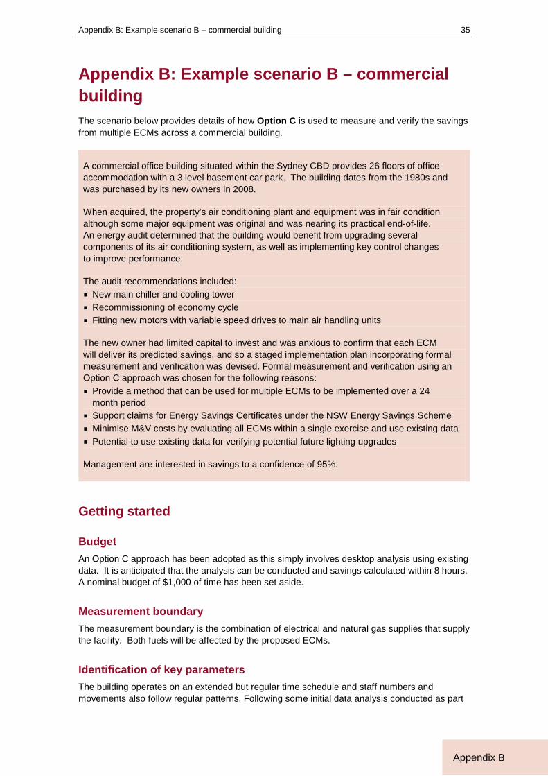
Appendix B: Example scenario B – commercial building The scenario below provides details of how Option C is used to measure and verify the savings from multiple ECMs across a commercial building.
A commercial office building situated within the Sydney CBD provides 26 floors of office accommodation with a 3 level basement car park. The building dates from the 1980s and was purchased by its new owners in 2008.
When acquired, the property’s air conditioning plant and equipment was in fair condition although some major equipment was original and was nearing its practical end-of-life. An energy audit determined that the building would benefit from upgrading several components of its air conditioning system, as well as implementing key control changes to improve performance.
The audit recommendations included: § New main chiller and cooling tower § Recommissioning of economy cycle § Fitting new motors with variable speed drives to main air handling units
The new owner had limited capital to invest and was anxious to confirm that each ECM will deliver its predicted savings, and so a staged implementation plan incorporating formal measurement and verification was devised. Formal measurement and verification using an Option C approach was chosen for the following reasons: § Provide a method that can be used for multiple ECMs to be implemented over a 24
month period § Support claims for Energy Savings Certificates under the NSW Energy Savings Scheme § Minimise M&V costs by evaluating all ECMs within a single exercise and use existing data § Potential to use existing data for verifying potential future lighting upgrades
Management are interested in savings to a confidence of 95%.
Getting started
Budget An Option C approach has been adopted as this simply involves desktop analysis using existing data. It is anticipated that the analysis can be conducted and savings calculated within 8 hours. A nominal budget of $1,000 of time has been set aside.
Measurement boundary The measurement boundary is the combination of electrical and natural gas supplies that supply the facility. Both fuels will be affected by the proposed ECMs.
Identification of key parameters The building operates on an extended but regular time schedule and staff numbers and movements also follow regular patterns. Following some initial data analysis conducted as part

Measurement and Verification Operational Guide
36
Appendix B
of the energy audit, the key parameters affecting electricity and natural gas usage was changes in ambient temperature.
The variables to be investigated are:
Variable Data source
Metered electricity and natural gas use Monthly electricity invoices
Ambient air temperature (heating and cooling degree days)
Daily figures for maximum and minimum air temperatures from the Bureau of Meteorology
Should these parameters fail to provide a suitable energy model, then additional parameters will be investigated.
Timing Baseline data was obtained from the previous owner and further baseline data was collected during late 2008/09 whilst preparations were made to implement the ECMs. The ECMs were implemented over 12 months commencing August 2009, and so the period just prior was chosen for the baseline. The baseline period consists of the 12 months between July 2008 and June 2009.
Interactive effects There are no interactive effects due to the choice of a facility based measurement boundary.
Summary of M&V plan The key elements of the project’s M&V plan in summary are:
Item Plan
Project Summary Implementation of the following ECMs on the base building air conditioning system: § new main chiller and cooling tower § recommissioning of economy cycle § fitting new motors with variable speed drives to main air handling units
Required Outcome To confirm savings with a 95% confidence level in order to support application for Energy Savings Certificates under the NSW Energy Savings Scheme.
Budget $1,000 (1 day of desktop analysis)
M&V Option C – Whole Facility The ESS application will be made using the Normalised Baseline method
Measurement Boundary Total incoming electrical and natural gas supplies being fed to 1540 Kent St, NSW.
Key Measurement Parameters
Data for the following key parameters will be collected and modelled in order to determine the most relevant factors affecting energy use: Metered electricity and natural gas use Ambient temperature (in the form of heating/cooling degree days)
Other Parameters to consider
Building occupancy – building occupancy has not changed during the last 3 years however major changes in the future may require additional modelling.
Potential interactive effects
None identified

Appendix B: Example scenario B – commercial building
37
Appendix B
Item Plan
Approach for conducting measurement and collecting data
Energy use data will be collected directly from energy invoices. Ambient temperature data will be sourced for the nearest weather station from the Bureau of Meteorology.
Measurement equipment required
Existing revenue meter and energy invoice data
Measurement period 12 month base year period, 1 month project implementation, and 12 month post-retrofit measurement.
Approach for calculating results
An energy model will be developed using regression analysis to explain baseline energy use in regard to relevant independent variables. Once the ECM has been implemented, post-retrofit data for these variables will be entered into the model in order to forecast the adjusted baseline or business-as-usual energy use. Savings are calculated by taking the difference in the adjusted baseline and actual energy use data on a monthly basis.
Baseline model development Microsoft Excel was chosen as the modelling tool. Two energy models will be developed as follows: 1. Electricity only model to be used to support ESS Application 4. Total energy model to be used for internal reporting
A spreadsheet was developed that contained the following elements: § Monthly baseline historical data for the key energy use parameters in independent variables § Daily weather maximum and minimum temperatures for the local weather station § HDDs and CDDs that have been derived from ambient temperature data, as described within
Section 6.5.2 within the Process Guide.
The baseline data is summarised below:
Month Energy use Electricity Only Ambient temperature
Total Energy Ambient temperature
Electricity (kWh)
Natural gas (MJ)
Total energy
(MJ)
HDDs Balance point =
n/a
CDDs Balance
point =18°C
HDDs Balance
point =18.45°C
CDDs Balance
point =13.6°C
B1 404,023 652,740 2,107,223 0 0 177 9
B2 378,914 638,848 2,002,938 0 0 177 7
B3 415,370 373,414 1,868,746 0 36 81 101
B4 468,311 37,021 1,722,941 0 56 36 166
B5 459,173 46,618 1,699,641 0 68 5 197
B6 520,358 0 1,873,289 0 124 1 260
B7 564,346 410 2,032,056 0 178 0 314
B8 510,519 2,461 1,840,329 0 132 0 255
B9 540,463 0 1,945,667 0 129 0 265
B10 419,802 46,910 1,558,197 0 50 15 169
B11 375,856 266,736 1,619,818 0 2 58 93
B12 339,846 419,441 1,642,887 0 0 132 26
12 months 5,396,981 2,484,599 21,913,731 0 774 681 1,865

Measurement and Verification Operational Guide
38
Appendix B
Each model was generated using the LINEST() function.
The LINEST() function is used to conduct multivariable linear regression on a dataset to produce a function describing y in terms of x1 to n in the form:
y = b + m1x1 + m2x2 + ...+ mnxn
where:
y = energy use
b = baseload energy use (without influence of any variables) – also known as y-intercept
x1 to n = data for independent variables 1 to n
m1 to n = coefficients determined by the function that correspond to each x variable
It accepts an array of y-values (i.e. energy use) and corresponding arrays of x-values (data for independent variables) and produces various outputs as shown below: § Coefficients and standard errors for the baseload energy use (b) and each independent
variable (m1 to n) § Coefficient of determination (R2), and Adjusted R2 which describe the ‘appropriateness of fit’
for the regression model § Standard error for y
Each model was tuned by using the “Solver” function that is available within the Analysis Tool pack within Microsoft Excel. Refer to Help within Microsoft Excel for further information for the LINEST() function and the “Solver” routine.
Preparing the weather data Weather data was downloaded from the Bureau of Meteorology website and imported into Excel. This is shown in columns C to K in the screenshot below.
The average daily temperature was calculated by averaging the daily maximum and minimum temperatures (Column L).
HDDs and CDDs were then calculated by determining the difference between the average daily temperature and the balance point (linked from another worksheet called “Energy Model”).

Appendix B: Example scenario B – commercial building
39
Appendix B
Separate calculations were performed for each model so that the most appropriate balance points can be determined independently.

Measurement and Verification Operation Guide
40
Appendix B
Developing the energy model using LINEST() The screenshot below presents the worksheet used to develop the energy model. Separate models were developed for Electricity based on CDDs and Total Energy based on both HDDs and CDDs.
The key elements of the worksheet are: § Baseline Data – derived from monthly energy invoices (Columns A to E)§ Balance points for calculating degree days (Rows 2 to 4) – these are values that are initially
entered and then adjusted (which in turn alters the number of HDDs and CDDs within each model) in order to maximise the correlation between ambient temperature and electricity/total energy use. § 2 energy models using the LINEST() function.
The key outputs of this function are highlighted below. In addition, the adjusted R2 value and the t-stats for each coefficient were calculated in order help validate each model.
coefficients
standard errors for coefficients standard error for y
R2
coefficients
standard errors for coefficients standard error for y R2

Appendix B: Example scenario B – commercial building
41
Appendix B
The output above equates to the following:
Model 1:
𝐸𝑙𝑒𝑐𝑡𝑟𝑖𝑐𝑖𝑡𝑦 𝑈𝑠𝑒 (𝑘𝑊ℎ) = 377,529.48 + 1119.96 × 𝐶𝐷𝐷𝑠
With a CDD balance point = 18 degrees Celsius
The R2 value is 0.933 and the standard error is 19,595.78.
Model 2:
𝑇𝑜𝑡𝑎𝑙 𝐸𝑛𝑒𝑟𝑔𝑦 𝑈𝑠𝑒 (𝑀𝐽) = 848,776.06 + 3,935.88 × 𝐶𝐷𝐷𝑠 + 6442.95 × 𝐻𝐷𝐷𝑠
With :
CDD balance point = 13.6 degrees Celsius
HDD balance point = 18.45 degrees Celsius
The R2 value is 0.845 whilst the Adjusted R2 is 0.811 and the standard error is 77,104.77.
Validating the regression outputs As described in Section 6.5.1, each model must be validated to confirm that it can be used. This involves equating some additional attributes and confirming their validity. The attributes to be reviewed are:
Attribute Description and Validity Test
R2 Must be 0.75 or higher. Output from LINEST() function
Adjusted R2
To be evaluated when multiple independent variables are used. Values should be 0.75 or higher. Calculated as follows:
𝐴𝑑𝑗𝑢𝑠𝑡𝑒𝑑 𝑅2 = 1 − (1 − 𝑅2) ×(𝑛 − 1)
(𝑛 − 𝑘 − 1)
Where: R2 = the value calculated from LINEST() n = number of data points in sample size k = number of coefficients within the regression model
t-statistic for each coefficient
Determine the validity of each x coefficient. Values must be greater than 2. Calculated as follows: Each ‘t-stat’ is calculated as follows:
𝑡𝑋𝑛 =𝑐𝑜𝑒𝑓𝑓𝑖𝑐𝑖𝑒𝑛𝑡𝑋𝑛
𝑠𝑡𝑎𝑛𝑑𝑎𝑟𝑑 𝑒𝑟𝑟𝑜𝑟𝑋𝑛

Measurement and Verification Operational Guide
42
Appendix B
Attribute Description and Validity Test
Absolute mean bias (MBE)
Determines the overall bias in the regression estimate. MBE values should be < 0.005%. Calculated as follows:
𝑀𝐵𝐸 =∑(𝑚𝑜𝑑𝑒𝑙𝑙𝑒𝑑𝑛 − 𝑎𝑐𝑡𝑢𝑎𝑙𝑛)
𝑛
Where: n = the number of samples modelledn = predicted value for sample item n actualn = actual value for sample item n
Monthly Mean Error CV(RMSE) Related to the standard error of the model. CV(RMSE) values should be < 0.25. Calculated as follows:
𝐶𝑉(𝑅𝑀𝑆𝐸) =𝑠𝑡𝑎𝑛𝑑𝑎𝑟𝑑 𝑒𝑟𝑟𝑜𝑟 𝑓𝑜𝑟 𝑦𝑎𝑣𝑒𝑟𝑎𝑔𝑒(𝑎𝑐𝑡𝑢𝑎𝑙 𝑣𝑎𝑙𝑢𝑒𝑠)
Validating Model 1
We calculate the following:
T-Stats:
𝑡𝐶𝐷𝐷𝑠 =1119.96289295.00792677
= 11.79
MBE:
MBE is calculated by first determining the modelled energy values by using the data for independent variables. Modelled values are then subtracted from actual values to calculate the difference for each measurement. These residuals are summed and divided by the number of data points to determine the MBE, as follows:
Month Actual electricity (kWh)
Modelled electricity (kWh)
Residual (modelled – actual) (kWh)
B1 404,023 377,529 -26,494
B2 378,914 377,529 -1,385
B3 415,370 417,512 2,142
B4 468,311 440,695 -27,616
B5 459,173 454,023 -5,150
B6 520,358 516,069 -4,289
B7 564,346 576,435 12,089
B8 510,519 525,197 14,678
B9 540,463 521,837 -18,626
B10 419,802 433,360 13,558
B11 375,856 379,265 3,409
B12 339,846 377,529 37,683
Sum 5,396,981 5,396,981 1.70 x 10⁻¹⁰
Average 449,748
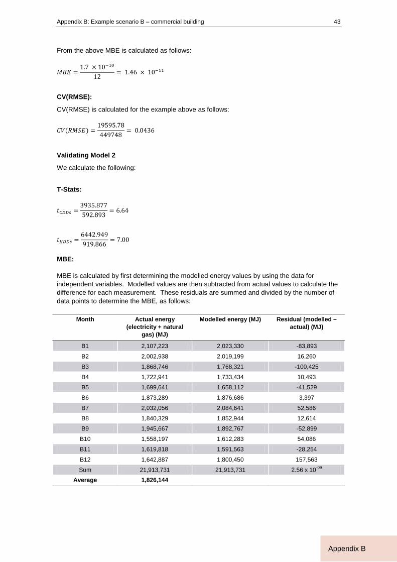
Appendix B: Example scenario B – commercial building
43
Appendix B
From the above MBE is calculated as follows:
𝑀𝐵𝐸 =1.7 × 10⁻¹⁰
12= 1.46 × 10⁻¹¹
CV(RMSE):
CV(RMSE) is calculated for the example above as follows:
𝐶𝑉(𝑅𝑀𝑆𝐸) =19595.78449748
= 0.0436
Validating Model 2
We calculate the following:
T-Stats:
𝑡𝐶𝐷𝐷𝑠 =3935.877592.893
= 6.64
𝑡𝐻𝐷𝐷𝑠 =6442.949919.866
= 7.00
MBE:
MBE is calculated by first determining the modelled energy values by using the data for independent variables. Modelled values are then subtracted from actual values to calculate the difference for each measurement. These residuals are summed and divided by the number of data points to determine the MBE, as follows:
Month Actual energy (electricity + natural
gas) (MJ)
Modelled energy (MJ) Residual (modelled – actual) (MJ)
B1 2,107,223 2,023,330 -83,893
B2 2,002,938 2,019,199 16,260
B3 1,868,746 1,768,321 -100,425
B4 1,722,941 1,733,434 10,493
B5 1,699,641 1,658,112 -41,529
B6 1,873,289 1,876,686 3,397
B7 2,032,056 2,084,641 52,586
B8 1,840,329 1,852,944 12,614
B9 1,945,667 1,892,767 -52,899
B10 1,558,197 1,612,283 54,086
B11 1,619,818 1,591,563 -28,254
B12 1,642,887 1,800,450 157,563
Sum 21,913,731 21,913,731 2.56 x 10-09
Average 1,826,144
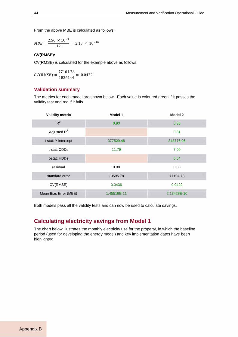
Measurement and Verification Operational Guide
44
Appendix B
From the above MBE is calculated as follows:
𝑀𝐵𝐸 =2.56 × 10⁻⁹
12= 2.13 × 10⁻¹⁰
CV(RMSE):
CV(RMSE) is calculated for the example above as follows:
𝐶𝑉(𝑅𝑀𝑆𝐸) =77104.781826144
= 0.0422
Validation summary The metrics for each model are shown below. Each value is coloured green if it passes the validity test and red if it fails.
Validity metric Model 1 Model 2
R2 0.93 0.85
Adjusted R2 0.81
t-stat: Y intercept 377529.48 848776.06
t-stat: CDDs 11.79 7.00
t-stat: HDDs 6.64
residual 0.00 0.00
standard error 19595.78 77104.78
CV(RMSE) 0.0436 0.0422
Mean Bias Error (MBE) 1.45519E-11 2.13428E-10
Both models pass all the validity tests and can now be used to calculate savings.
Calculating electricity savings from Model 1 The chart below illustrates the monthly electricity use for the property, in which the baseline period (used for developing the energy model) and key implementation dates have been highlighted.

Appendix B: Example scenario B – commercial building
45
Appendix B
The trendline shown in Orange forecasts the monthly energy consumption for ‘business as usual’ based on the energy model that has been developed. Savings can now be calculated simply by subtracting the actual electricity use (shown in black) from the forecast.
This data is listed in the table below.
Month Actual Electricity Use (kWh)
CDDs Adjusted Baseline (kWh)
Savings (kWh)
P1 295,194 0 377,529 82,335
P2 302,304 0 377,529 75,225
P3 309,246 11 389,345 80,099
P4 323,011 35 416,280 93,269
P5 369,061 75 460,967 91,906
P6 396,045 135 529,228 133,183
P7 434,738 190 590,266 155,528
P8 430,390 190 590,210 159,820
P9 438,535 142 536,788 98,253
P10 312,149 29 410,288 98,139
P11 305,246 1 378,929 73,683
P12 282,111 1 378,145 96,034
Total 12 months 4,198,030 808 5,435,508 1,237,478
0
100,000
200,000
300,000
400,000
500,000
600,000
700,000El
ectri
city
Use
(kW
h)actual model
Baseline Period Air handlers retrofitted
New chiller installed
Economy Cycle recommissioned

Measurement and Verification Operational Guide
46
Appendix B
Uncertainty analysis for Model 1 As shown earlier, the standard error (SE) of the baseline energy model is:
𝑠𝑡𝑎𝑛𝑑𝑎𝑟𝑑 𝑒𝑟𝑟𝑜𝑟(𝑆𝐸) = 19595.78 𝑘𝑊ℎ
Using the standard error we can calculate the absolute precision (AP) by applying the t-statistic for our chosen sample size (DF = 12 data points – 1 variable – 1 = 10) and required confidence (95%).
𝐴𝑏𝑠𝑜𝑙𝑢𝑡𝑒 𝑝𝑟𝑒𝑐𝑖𝑠𝑖𝑜𝑛 (𝐴𝑃) = 𝑡 × 𝑆𝐸
𝐴𝑏𝑠𝑜𝑙𝑢𝑡𝑒 𝑝𝑟𝑒𝑐𝑖𝑠𝑖𝑜𝑛 (𝐴𝑃) = 2.23 × 19595.78 = 43,699 𝑘𝑊ℎ
And the relative precision (RP) is calculated by dividing the absolute precision by the average predicted energy use as follows:
𝑟𝑒𝑙𝑎𝑡𝑖𝑣𝑒 𝑝𝑟𝑒𝑐𝑖𝑠𝑖𝑜𝑛 (𝑅𝑃) =𝐴𝑃
𝑎𝑣𝑒𝑟𝑎𝑔𝑒 𝑚𝑜𝑛𝑡ℎ𝑙𝑦 𝑚𝑜𝑑𝑒𝑙𝑙𝑒𝑑 𝑢𝑠𝑎𝑔𝑒
𝑟𝑒𝑙𝑎𝑡𝑖𝑣𝑒 𝑝𝑟𝑒𝑐𝑖𝑠𝑖𝑜𝑛 (𝑅𝑃) =43699 449748
= ±9.7%
The uncertainty of the savings is calculated as follows:
𝑆𝐸(𝑚𝑜𝑛𝑡ℎ𝑙𝑦 𝑠𝑎𝑣𝑖𝑛𝑔𝑠) = �𝑆𝐸(𝑎𝑑𝑗𝑢𝑠𝑡𝑒𝑑 𝑏𝑎𝑠𝑒𝑙𝑖𝑛𝑒)2 + 𝑆𝐸(𝑝𝑜𝑠𝑡 𝑟𝑒𝑡𝑟𝑜𝑓𝑖𝑡)2
= �19595.782 + 02 = 19595.78 𝑘𝑊ℎ
Assuming that the standard error of each month’s savings will be the same, the standard error for the annual savings is:
𝑆𝐸(𝑎𝑛𝑛𝑢𝑎𝑙 𝑠𝑎𝑣𝑖𝑛𝑔𝑠) = �12 × 19595.782 = 67881.76 𝑘𝑊ℎ
Using a t-statistic of 2.20 (12 measurement points with 95% confidence), the range of possible annual savings will be:
𝑅𝑎𝑛𝑔𝑒 𝑜𝑓 𝑆𝑎𝑣𝑖𝑛𝑔𝑠 (𝑘𝑊ℎ) = 1237478 ± 2.20 × 67881.76 𝑘𝑊ℎ
= 1,237,478 ± 149,340 𝑘𝑊ℎ
The relative precision of the annual savings reported is thus ±12.1% (149,340 / 1,237,478)
Reporting results from Model 1 The savings results can be described by the following:
The annual savings are calculated to be 1,237,478 kWh ± 12.1% or 149,340 kWh with a 95% confidence factor.
Savings fall within the range of 1,088,138 kWh to 1,386,818 kWh.

Appendix B: Example scenario B – commercial building
47
Appendix B
Using this result, the property owner is able to suitably demonstrate a robust M&V methodology within its ESS Application to support its Energy Savings Certificates claim.
Reporting results from Model 2 Using similar techniques, the total energy savings determined by Model 2 are found as follows:
Month Actual Electricity Use
(MJ)
HDDs CDDs Adjusted Baseline (MJ)
Savings (MJ)
P1 1,833,621 165 12 1,956,838 123,217
P2 1,684,046 142 23 1,854,236 170,190
P3 1,307,465 63 91 1,610,976 303,512
P4 1,202,624 28 150 1,615,659 413,036
P5 1,333,753 12 198 1,701,905 368,153
P6 1,425,762 1 271 1,923,864 498,102
P7 1,565,057 0 326 2,133,250 568,193
P8 1,549,404 0 313 2,081,099 531,695
P9 1,579,171 0 279 1,946,278 367,107
P10 1,123,800 13 154 1,535,922 412,122
P11 1,283,828 105 51 1,722,919 439,092
P12 1,244,207 129 28 1,788,582 544,375
Total 12 months 17,132,737 656 1,895 21,871,529 4,738,792
The savings results can be described by the following:
The annual savings are calculated to be 4,738,792 MJ ± 12.4% or 587,617 MJ with a 95% confidence factor.
Savings fall within the range of 4,151,175 MJ to 5,326,409 MJ.
More simply, the annual savings are calculated to be 4,739 GJ ± 12%.