Measurement and fusion ofnon-invasive vital signs for routinetriage of acute paediatric illness

Susannah FlemingKeble College

Supervised by: Professor Lionel TarassenkoTrinity Term, 2010

This DPhil Thesis is submitted to theDepartment of Engineering Science, University of Oxford

Measurement and fusion of non-invasive vital signs for routinetriage of acute paediatric illness

Susannah FlemingKeble College

DPhil in Engineering ScienceTrinity Term, 2010

Abstract

Serious illness in childhood is a rare occurrence, but accounts for 20% of childhooddeaths. Early recognition and treatment of serious illness is vital if the child is to recoverwithout long-term disability. It is known that vital signs such as heart rate, respiratoryrate, temperature, and oxygen saturation can be used to identify children who are at highrisk of serious illness.

This thesis presents research into the development of a vital signs monitor, designedfor use in the initial assessment of unwell children at their first point of contact with amedical practitioner. Child-friendly monitoring techniques are used to obtain vital signs,which can then be combined using data fusion techniques to assist clinicians in identifyingchildren with serious illenss.

Existing normal ranges for heart rate and respiratory rate in childhood vary consider-ably, and do not appear to be based on clinical evidence. This thesis presents a systematicmeta-analysis of heart rate and respiratory rate from birth to 18 years of age, providingevidence-based curves which can be used to assess the degree of abnormality in theseimportant vital signs.

Respiratory rate is particularly difficult to measure in children, but is known to bepredictive of serious illness. Current methods of automated measurement can be distress-ing, or are time-consuming to apply. This thesis therefore presents a novel method forestimating the respiratory rate from an optical finger sensor, the pulse oximeter, which isroutinely used in clinical practice.

Information from multiple vital signs can be used to identify children at risk of seriousillness. A number of data fusion techniques were tested on data collected from childrenattending primary and emergency care, and shown to outperform equivalent existingscoring systems when used to identify those with more serious illness.

i

Acknowledgements

First and foremost, I must thank my supervisor, Professor Lionel Tarassenko, for his

support, enthusiasm, and encouragement throughout this research. Thanks are also due

to my clinical collaborators in the Department of Primary Health Care, and particularly

to Dr Matthew Thompson and Professor David Mant, who have supported this project

from the start, and who assisted with the collection of data from the Oxford School Study.

I would also like to thank the EPSRC and NIHR, without whose funding this research

would not have taken place.

The meta-analysis in Chapter 2 would not have been possible without the assistance

of Richard Stevens, who had the initial idea for modifying the kernel regression method to

take age ranges and sample sizes into account, and who also provided invaluable statistical

support for the data fusion work in Chapter 6. I would also like to thank Annette

Pluddemann for volunteering to carry out the vital, but time-consuming task of going

through all 69 papers to double-check my data entry and paper descriptions. I am grateful

to Dr Carl Heneghan and Dr Ian Maconochie for their comments and criticism on the

meta-analysis in Chapter 2, which much improved its clinical relevance.

I would like to thank Nia Roberts for carrying out the literature search required

for Chapter 2, and the librarians at the Health Care libraries, Radcliffe Science library,

and British library for their invaluable assistance in locating obscure, and occasionally

mis-catalogued, journals. Thanks are also due to my translators: Sam Hugueny, Ibrat

Djabbarov, Lei Clifton, Claudine Neyen, Rafael Perera, and Annette Pluddemann, and

to Michael Stewart for providing access to his copy of the Advanced Trauma Life Support

student’s manual when I was starting to give up hope of ever finding a copy.

Special thanks are due to Sarah Nash, and the staff and students of St Michael’s

CE Primary School in Oxford, for allowing me to invade their library and carry out the

measurements for the Oxford School Study; and to the staff and patients at the Oxford

Emergency Medical Service, for their assistance with the data collection for the OXEMS

study.

I am grateful for the friendship and assistance of all my colleagues in the Biomedical

Signal Processing group. Particular thanks go to David Clifton, who assisted with the

ii

development of the jack-knifing method described in Chapter 6, and developed the outlier

pruning method described in Appendix B.7; and Alistair Hann, who took me under his

wing as a new DPhil student, and inducted me into the joys of working with clinical

data. I would also like to extend special thanks to Val Mitchell, who has been a font of

knowledge regarding administration and paperwork, and who kept me sane in the face of

unexpectedly looming deadlines.

The journey to this thesis started with Gareth Smith, who suggested that I apply to

do a DPhil at the Life Sciences Interface Doctoral Training Centre. I would like to extend

my thanks to all the DTC staff and students who supported me through my DPhil, and

particularly to Maureen York, who kept us in line and motivated.

Performing DPhil research and writing a thesis can be stressful and demoralising.

Special thanks are therefore due to all those who supported me throughout the last four

years. It would be impossible to list everyone here, but I would like to extend particular

thanks to everybody from Keble Chapel and St Mary Magdalen’s for your prayers and

friendship. I would also like to thank Michael, Gareth and Miles for commiserating over

thesis woes; Kake for proof-reading; Nautilus for providing friendly crash space when I

needed to be in London; Alia for enticing me away from work to do filming; Claire and

Andy for organising holidays; Cub for. . . being Cub; and all the Scoobies for putting up

with me and sending virtual (and occasional real) hugs, tea and chocolate when things

were tough.

Finally, I would like to thank my parents, Pat and Bernard Fleming, and all my

family, for their never-ending support and encouragement, their willingness to listen to

me wittering on about my research, and for bringing me back to reality and reminding

me not to get “boffinised”.

iii

Contents

1 Introduction 11.1 Assessing the severity of illness using vital signs . . . . . . . . . . . . . . . 3

1.1.1 Using triage to assess patients in emergency care . . . . . . . . . . 41.1.2 Monitoring children during hospital care . . . . . . . . . . . . . . . 61.1.3 Assessing children in primary care . . . . . . . . . . . . . . . . . . . 10

1.2 Monitoring vital signs in children . . . . . . . . . . . . . . . . . . . . . . . 111.2.1 Heart rate . . . . . . . . . . . . . . . . . . . . . . . . . . . . . . . . 121.2.2 Respiratory rate . . . . . . . . . . . . . . . . . . . . . . . . . . . . . 141.2.3 Arterial oxygen saturation (SpO2) . . . . . . . . . . . . . . . . . . . 171.2.4 Temperature . . . . . . . . . . . . . . . . . . . . . . . . . . . . . . . 211.2.5 Capillary refill time / peripheral perfusion . . . . . . . . . . . . . . 22

1.3 Overview of thesis – proposed vital sign instrumentation . . . . . . . . . . 24

2 Age correction of heart rate and respiratory rate in children 262.1 Methods . . . . . . . . . . . . . . . . . . . . . . . . . . . . . . . . . . . . . 29

2.1.1 Literature search . . . . . . . . . . . . . . . . . . . . . . . . . . . . 292.1.2 Data extraction . . . . . . . . . . . . . . . . . . . . . . . . . . . . . 312.1.3 Data analysis . . . . . . . . . . . . . . . . . . . . . . . . . . . . . . 34

2.2 Results . . . . . . . . . . . . . . . . . . . . . . . . . . . . . . . . . . . . . . 372.2.1 Heart rate . . . . . . . . . . . . . . . . . . . . . . . . . . . . . . . . 382.2.2 Respiratory rate . . . . . . . . . . . . . . . . . . . . . . . . . . . . . 42

2.3 Proposed age correction method for heart rate and respiratory rate . . . . 442.3.1 Performance of age correction methods on data from primary and

emergency care . . . . . . . . . . . . . . . . . . . . . . . . . . . . . 452.4 Conclusions . . . . . . . . . . . . . . . . . . . . . . . . . . . . . . . . . . . 49

3 Measuring respiratory rate using the finger probe (PPG) 503.1 Introduction . . . . . . . . . . . . . . . . . . . . . . . . . . . . . . . . . . . 503.2 Physiological basis of breathing information in the PPG . . . . . . . . . . . 51

3.2.1 Amplitude-modulated breathing signals . . . . . . . . . . . . . . . . 513.2.2 Frequency-modulated breathing signals . . . . . . . . . . . . . . . . 52

3.3 Signal processing for respiratory rate extraction from the PPG . . . . . . . 543.3.1 Extraction of amplitude-modulated signals . . . . . . . . . . . . . . 543.3.2 Extraction of frequency-modulated signals . . . . . . . . . . . . . . 57

3.4 Summary of methods . . . . . . . . . . . . . . . . . . . . . . . . . . . . . . 61

4 Accuracy of respiratory rate estimation in adults 644.1 Introduction . . . . . . . . . . . . . . . . . . . . . . . . . . . . . . . . . . . 644.2 Testing procedure . . . . . . . . . . . . . . . . . . . . . . . . . . . . . . . . 65

4.2.1 Windowing of data . . . . . . . . . . . . . . . . . . . . . . . . . . . 654.2.2 Quality metric . . . . . . . . . . . . . . . . . . . . . . . . . . . . . . 66

iv

4.3 Measuring breathing from the amplitude modulation of the PPG . . . . . . 674.3.1 Digital filtering . . . . . . . . . . . . . . . . . . . . . . . . . . . . . 674.3.2 Fourier transforms . . . . . . . . . . . . . . . . . . . . . . . . . . . 714.3.3 Continuous wavelet transforms . . . . . . . . . . . . . . . . . . . . . 744.3.4 Autoregressive modelling . . . . . . . . . . . . . . . . . . . . . . . . 784.3.5 Autoregressive modelling with Kalman filtering . . . . . . . . . . . 824.3.6 Summary of results for methods using amplitude modulation . . . . 84

4.4 Measuring breathing from frequency modulation of the PPG . . . . . . . . 854.4.1 Tachogram generation . . . . . . . . . . . . . . . . . . . . . . . . . 854.4.2 Digital filtering . . . . . . . . . . . . . . . . . . . . . . . . . . . . . 884.4.3 Autocorrelation function . . . . . . . . . . . . . . . . . . . . . . . . 894.4.4 Autoregressive modelling . . . . . . . . . . . . . . . . . . . . . . . . 924.4.5 Autoregressive modelling with Kalman filtering . . . . . . . . . . . 934.4.6 Summary of results from methods using frequency modulation . . . 94

4.5 Summary . . . . . . . . . . . . . . . . . . . . . . . . . . . . . . . . . . . . 96

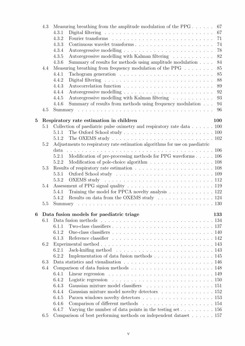
5 Respiratory rate estimation in children 1005.1 Collection of paediatric pulse oximetry and respiratory rate data . . . . . . 100

5.1.1 The Oxford School study . . . . . . . . . . . . . . . . . . . . . . . . 1005.1.2 The OXEMS study . . . . . . . . . . . . . . . . . . . . . . . . . . . 102

5.2 Adjustments to respiratory rate estimation algorithms for use on paediatricdata . . . . . . . . . . . . . . . . . . . . . . . . . . . . . . . . . . . . . . . 1065.2.1 Modification of pre-processing methods for PPG waveforms . . . . . 1065.2.2 Modification of pole-choice algorithm . . . . . . . . . . . . . . . . . 108

5.3 Results of respiratory rate estimation . . . . . . . . . . . . . . . . . . . . . 1085.3.1 Oxford School study . . . . . . . . . . . . . . . . . . . . . . . . . . 1095.3.2 OXEMS study . . . . . . . . . . . . . . . . . . . . . . . . . . . . . 112

5.4 Assessment of PPG signal quality . . . . . . . . . . . . . . . . . . . . . . . 1195.4.1 Training the model for PPCA novelty analysis . . . . . . . . . . . . 1225.4.2 Results on data from the OXEMS study . . . . . . . . . . . . . . . 124

5.5 Summary . . . . . . . . . . . . . . . . . . . . . . . . . . . . . . . . . . . . 130

6 Data fusion models for paediatric triage 1336.1 Data fusion methods . . . . . . . . . . . . . . . . . . . . . . . . . . . . . . 134

6.1.1 Two-class classifiers . . . . . . . . . . . . . . . . . . . . . . . . . . . 1376.1.2 One-class classifiers . . . . . . . . . . . . . . . . . . . . . . . . . . . 1406.1.3 Reference classifier . . . . . . . . . . . . . . . . . . . . . . . . . . . 142

6.2 Experimental method . . . . . . . . . . . . . . . . . . . . . . . . . . . . . . 1436.2.1 Jack-knifing method . . . . . . . . . . . . . . . . . . . . . . . . . . 1436.2.2 Implementation of data fusion methods . . . . . . . . . . . . . . . . 145

6.3 Data statistics and visualisation . . . . . . . . . . . . . . . . . . . . . . . . 1466.4 Comparison of data fusion methods . . . . . . . . . . . . . . . . . . . . . . 148

6.4.1 Linear regression . . . . . . . . . . . . . . . . . . . . . . . . . . . . 1496.4.2 Logistic regression . . . . . . . . . . . . . . . . . . . . . . . . . . . 1506.4.3 Gaussian mixture model classifiers . . . . . . . . . . . . . . . . . . 1516.4.4 Gaussian mixture model novelty detectors . . . . . . . . . . . . . . 1526.4.5 Parzen windows novelty detectors . . . . . . . . . . . . . . . . . . . 1536.4.6 Comparison of different methods . . . . . . . . . . . . . . . . . . . 1546.4.7 Varying the number of data points in the testing set . . . . . . . . . 156

6.5 Comparison of best performing methods on independent dataset . . . . . . 157

v

6.6 Addition of respiratory rate . . . . . . . . . . . . . . . . . . . . . . . . . . 1606.7 Predictivity of individual vital signs . . . . . . . . . . . . . . . . . . . . . . 1626.8 Summary . . . . . . . . . . . . . . . . . . . . . . . . . . . . . . . . . . . . 164

7 Conclusions 1677.1 Overview . . . . . . . . . . . . . . . . . . . . . . . . . . . . . . . . . . . . . 1677.2 Further work . . . . . . . . . . . . . . . . . . . . . . . . . . . . . . . . . . 169

7.2.1 Validation of meta-analysis results . . . . . . . . . . . . . . . . . . 1697.2.2 Improvement of respiratory rate estimation using the PPG . . . . . 1707.2.3 Data fusion of vital signs . . . . . . . . . . . . . . . . . . . . . . . . 172

7.3 Proposed follow-up study . . . . . . . . . . . . . . . . . . . . . . . . . . . . 172

A Sources of data 197A.1 Data for testing respiratory rate extraction methods . . . . . . . . . . . . . 198

A.1.1 Data from the MIMIC database . . . . . . . . . . . . . . . . . . . . 198A.1.2 Data from the Controlled Breathing database . . . . . . . . . . . . 200A.1.3 Paediatric data from Oxford School Study . . . . . . . . . . . . . . 206A.1.4 Paediatric data from OXEMS Study . . . . . . . . . . . . . . . . . 211

A.2 Paediatric vital signs data from primary and emergency care . . . . . . . . 212A.2.1 The Fever and Tachycardia dataset . . . . . . . . . . . . . . . . . . 213A.2.2 The Walsgrave dataset . . . . . . . . . . . . . . . . . . . . . . . . . 213A.2.3 The combined FW dataset . . . . . . . . . . . . . . . . . . . . . . . 214A.2.4 Using the datasets for data fusion . . . . . . . . . . . . . . . . . . . 214

B Mathematical Methods 215B.1 Kernel regression . . . . . . . . . . . . . . . . . . . . . . . . . . . . . . . . 215

B.1.1 Classic kernel regression . . . . . . . . . . . . . . . . . . . . . . . . 215B.1.2 Weighted variable bandwidth kernel regression . . . . . . . . . . . . 218

B.2 Simple breath detection algorithm . . . . . . . . . . . . . . . . . . . . . . . 219B.3 Autoregressive modelling . . . . . . . . . . . . . . . . . . . . . . . . . . . . 220B.4 Kalman filtering . . . . . . . . . . . . . . . . . . . . . . . . . . . . . . . . . 222B.5 Probabilistic principal component analysis . . . . . . . . . . . . . . . . . . 223B.6 Novelty detection using multivariate extreme value theory . . . . . . . . . 225B.7 Pruning of outliers using GMMs . . . . . . . . . . . . . . . . . . . . . . . . 227

C Data from literature search 229C.1 Search terms . . . . . . . . . . . . . . . . . . . . . . . . . . . . . . . . . . . 229C.2 Reasons for exclusion of articles . . . . . . . . . . . . . . . . . . . . . . . . 231C.3 Summary of included papers . . . . . . . . . . . . . . . . . . . . . . . . . . 232

D Tables of normal heart rate and respiratory rate 240

vi

Chapter 1

Introduction

Children account for around 25% of all GP1 consultations and Emergency Department2

visits in the UK (Saxena et al., 1999; Pearson, 2008). Of children who present with

acute medical illness, 40–50% will have respiratory difficulties or infectious illnesses (Ar-

mon et al., 2001; Saxena et al., 1999). Although serious illnesses such as meningitis or

pneumonia are rare, occurring in less than 10% of cases of illness in children, they are

responsible for 20% of deaths in childhood, and require early recognition and treatment to

give the best chance of a full recovery (Saxena et al., 1999; Stewart et al., 1998; Pearson,

2008).

Differentiating serious illness from minor or self-limiting conditions can be difficult,

particularly in the early stages of the disease. For example, a study of children with

meningococcal disease showed that only half were referred to hospital at their first contact

with a GP (Thompson et al., 2006). A report into the causes of death in children (Pearson,

2008) determined that 26% of childhood deaths are avoidable. It identified “failure to

recognise severity of illness” as a major contributor to avoidable death, and recommended

the adoption of “early identification systems for children developing critical illness”.

The UK National Institute for Health and Clinical Excellence (NICE) guidelines on

treating children with feverish illness recommend that “healthcare professionals should

measure and record temperature, heart rate, respiratory rate, and capillary refill time as

1A GP, or general practitioner, is a community-based doctor who provides routine care, and acts asan initial point of contact for patients requiring medical advice or treatment.

2An Emergency Department (ED) is a hospital department providing urgent assessment and treatmentof serious illnesses and injuries. Alternative names include Casualty, Accident and Emergency (A&E),and Emergency Room (ER).

1

part of the routine assessment” (National Collaborating Centre for Women’s and Chil-

dren’s Health, 2007), as abnormalities in these vital signs are known to be associated with

severe illness in children (Margolis and Gadomski, 1998; Chamberlain et al., 1998; Pollack

et al., 1997). However, general practitioners do not appear to measure these physiological

parameters frequently, even though they accept that vital signs are valuable in assessing

the severity of infection and respiratory illness (Thompson et al., 2008). Possible reasons

for this include the difficulty of measurement, and poor understanding of what consti-

tutes an abnormal value in children, especially as what constitutes a normal value for

some parameters will vary with the child’s age.

Respiratory rate is recognised as a particularly useful vital sign for predicting serious

illness in children. An increased respiratory rate is predictive of the presence of pneumonia

(Margolis and Gadomski, 1998), admission to hospital (Chamberlain et al., 1998), and

death (Pollack et al., 1997). However, it is only measured regularly by 17% of general

practitioners (Thompson et al., 2008). This is likely to be due in part to the difficult

and time-consuming nature of manual respiratory rate measurement in children, and

a recognition that manual measurement can be highly inaccurate (Lovett et al., 2005;

Simoes et al., 1991). If respiratory rate is to be measured manually, the number of breaths

should be counted over a minimum of 60 seconds, as this ensures an acceptable level of

accuracy in the calculated rate, allowing the clinician to discriminate between a normal

respiratory rate and one that is abnormally fast or slow, which might not be possible if a

shorter measurement period was used (Simoes et al., 1991). However, such a long period

of measurement may be perceived as an inefficient use of the limited consultation time

available to clinicians in a primary care environment.

Primary care is typically the first point of contact for patients, and is usually located in

the community. It includes GP surgeries, pharmacists, and other community-based health

care professionals, such as health visitors or community midwives. Medical treatment may

also be provided in the context of secondary or tertiary care. Secondary care typically

provides more specialist assessment and treatment than primary care, and takes place in

a hospital environment. With the exception of the Emergency Department, secondary

care will usually require a referral from a primary care practitioner. Tertiary care is used

2

to denote further specialised services receiving referrals from both primary and secondary

care. The definitions of secondary and tertiary care overlap somewhat, but tertiary care

typically serves a geographic area containing multiple secondary care providers, e.g. burns

units, and spinal rehabilitation centres.

This thesis describes the development of a system to identify seriously ill children in

the primary care environment, using non-invasive3 measurements of vital signs such as

heart rate, respiratory rate, and temperature. In this context, the vital sign monitoring

would be initiated by a clinician (e.g. a nurse or doctor), and analysed by a computer

to assess the severity of the illness. This result could then be used by the clinician in

conjunction with other information to make a diagnosis and/or determine a course of

treatment.

Although the intended application of the system is the primary care environment,

the problem of identifying serious illness is also present in secondary care environments.

Some techniques used in secondary care may therefore inform the development of a tool

for use in primary care, provided that the limitations of the primary care environment

are considered.

1.1 Assessing the severity of illness using vital signs

In the hospital environment, various methods may be employed to assess the severity

of illness, depending on the particular care setting (e.g. emergency department, general

ward, or intensive care unit). The assessment of illness in the emergency department (ED)

has strong similarities with that carried out in primary care, as patients may not have

been medically assessed before arrival, and so there is often no prior information as to

the severity of their illness. However, there are also similarities with monitoring methods

employed on wards, which aim to identify those patients who require additional clinical

input to prevent deterioration. Since both of these systems contain elements that would

be informative for the development of a system to identify acute illness in primary care,

they are investigated further in this section.

3Non-invasive measurements do not break the skin or involve the insertion of instruments into a bodycavity.

3

1.1.1 Using triage to assess patients in emergency care

The method used to assess the severity of illness (and injury) in emergency departments is

known as triage. The word “triage” derives from the French verb trier, meaning to pick or

cull (OED Online, 1989). In the medical context, triage is the process of sorting patients

into groups, and assigning priorities to these groups. Triage is typically used where the

demand for resources outstrips supply, and usually involves assigning the highest priority

to the most seriously ill patients (Nocera and Garner, 1999).

In the civilian medical context, triage is used to assign priorities in emergency care

(ambulance service and emergency departments); and at the scene of mass casualty inci-

dents. Triage algorithms are therefore designed with these applications in mind.

Triage systems designed for classifying adults should not be used to assess children

unless they have been modified to take into account the different priorities that should be

assigned to children and adults displaying the same symptoms. This is because children

are not simply “small adults”; their physiology means that they will tend to be overtriaged

(given an excessively high priority) by systems which use vital sign limits designed for use

on adults (Wallis and Carley, 2006). In addition, certain complaints, such as fever and

abdominal pain, can be a concerning finding in children, but would not generally indicate

serious illness in an adult (O’Neill and Molczan, 2003). Modern triage systems manage

this problem by either incorporating modifications such as child-specific flow charts, or

by using a separate paediatric triage system derived from the adult system, as is the case

with the Canadian Triage and Acuity Scale (CTAS), which has a separate Paed-CTAS

version for use in children (Gouin et al., 2005).

The triage process

Triage typically occurs as soon as a patient presents to the service, such as an emergency

department. Existing triage systems use between two and seven priority levels, with the

discrimination being based on symptoms, risk factors, vital signs, test results and likely

utilisation of clinical resources (Beveridge, 1998). An ideal triage system should be able

to predict outcomes such as mortality, hospitalisation and resource use, and should give

reproducible results, so that the same patient triaged by two different observers would be

4

assigned the same triage category.

No triage system is perfect, and it is inevitable that some patients will be assigned a

priority that does not truly reflect the severity of their condition. Undertriage, whereby a

patient receives a lower triage priority than their condition demands, puts the undertriaged

patient at risk, as they may suffer adverse consequences due to a delay in receiving

appropriate treatment. The opposite problem, overtriage, whereby patients are assigned

an excessively high priority, is not necessarily dangerous to the overtriaged patient, but

may adversely affect other patients as resources are unnecessarily diverted from those who

require them. There is some evidence that current triage algorithms tend to overtriage

paediatric patients, particularly those who present with febrile illness (Maldonado and

Avner, 2004; Roukema et al., 2006).

Triage of adult and paediatric patients in the Emergency Department

Triage in the emergency department is not necessarily limited to assigning treatment

priorities, with triage nurses frequently being empowered to initiate treatment and order

diagnostic tests if appropriate (O’Neill and Molczan, 2003).

Many modern triage systems, including the Australasian Triage Scale (ATS), Cana-

dian Triage and Acuity Scale (CTAS), Manchester Triage Scale (MTS), and the Soterion

Rapid Triage System (SRTS) use a similar methodology (Scoble, 2004; Gouin et al., 2005;

Durojaiye and O’Meara, 2002; Maningas et al., 2006). These scales use a combination of

vital sign measurements and complaint-specific flow charts to assign a triage level. These

systems may be computerised, paper-based, or a combination, depending on the needs of

the clinical environment.

Other systems, such as the Emergency Severity Index (ESI), use a combination of vital

signs and the predicted resources (such as diagnostic tests and medical interventions) that

will be required by a patient to assign treatment priorities (Gilboy et al., 2005).

In the absence of a specific paediatric scale, such as the Paed-CTAS system (Gouin

et al., 2005), paediatric patients can be incorporated into existing systems by introducing

age-dependent limits for vital sign measurements. In the case of systems which use flow

charts, it is also necessary to introduce child-specific flow charts or paediatric modifications

5

to existing flow charts. The triage of paediatric patients can also depend on the paediatric

experience of the triage nurse, with evidence that nurses based in mixed departments

(treating both adults and children) tend to assign higher triage priorities to children than

those working in paediatric emergency departments, particularly when the child has a

fever (Durojaiye and O’Meara, 2002; Maldonado and Avner, 2004).

1.1.2 Monitoring children during hospital care

Monitoring of various parameters is carried out in all hospital care settings with the aim of

detecting changes in the physiological state of the patient. Ideally, such changes should be

detected in time to allow interventions to be carried out to stabilise the patient’s condition

and prevent any further deterioration. Various methods have been proposed for identifying

those children who are at high risk of deterioration or require urgent intervention.

Predicting outcomes in paediatric populations

The earliest methods for identifying serious illness in children were developed for use in

the paediatric intensive care unit (PICU), where the most unwell children are treated

(Yeh et al., 1984; Pollack et al., 1996). These methods rely on the measurement of

many variables, including blood tests and invasive measurements, which may only be

available for patients being cared for on such specialist units. This type of score is typically

developed by assessing the risk of a given outcome, such as mortality or admission, in a

population of patients, and so the output of the score can often be converted to obtain

an odds ratio4 for the relevant outcome.

The use of this type of score is no longer restricted to the intensive care setting, as

scores such as the Pediatric Risk of Admission (PRISA) and the Pediatric Emergency

Assessment Tool (PEAT) also use this methodology to predict the risk of a child being

admitted as an in-patient after attending the Emergency Department (Chamberlain et al.,

1998; Gorelick et al., 2001). As fewer physiological measurements are typically available

for Emergency Department patients, these scores also take into account other factors

4The odds ratio is a ratio of probabilites, and can be interpreted as the number of times as likely anoutcome is. For example, if the probability of dying for a patient is 0.8, the odds ratio for that outcomewill be 0.8

1−0.8 = 4; i.e. the patient is 4 times more likely to die than to survive.

6

such as demographic data, medical history, and the type of treatment required during the

Emergency Department consultation.

Score Prediction Method Variables ComponentsPSI (Yehet al., 1984)

severity ofillness inPICU

additive scoredesigned byclinicians

34 4 vital signs, 4 cardiacindices, 22 blood testsand 4 neurological ob-servations

PRISM-III(Pollacket al., 1996)

mortality inPICU

additive scoredesigned usinglogisticregression

17 3 vital signs, 12 bloodtests and 2 neurologi-cal observations

PRISA(Chamberlainet al., 1998)

admissionfrom ED

additive scoredesigned usinglogisticregression

21 5 vital signs, 3 bloodtests, 1 neurologicalobservation, 3 demo-graphics, 3 medicalhistory, 2 therapies, 4interactions

PEAT(Gorelicket al., 2001)

level of carefrom ED

logisticregression model

8 3 vital signs, 2 de-mographics, 1 medicalhistory, 2 diagnosis

PIM2 (Slateret al., 2003)

mortality inPICU

logisticregression model

10 1 vital sign, 2 bloodtests, 1 neurologicalobservation, 2 demo-graphics, 2 therapies,2 medical history

RePEAT(Gorelicket al., 2007)

level of carefrom ED

logisticregression model

8 3 vital signs, 2 de-mographics, 1 medicalhistory, 2 diagnosis

Table 1.1: Summary of the design of six scores used to predict outcomes in paediatricpopulations. Abbreviations used: PICU (paediatric intensive care unit); ED (Emergencydepartment)

Table 1.1 summarises the design of six scores used to predict outcomes in children. Of

these scores, only the PEAT and RePEAT can be calculated entirely using variables that

would be available outside the hospital setting, as the other scores all require the results of

blood testing to calculate. Although blood samples for these tests can be taken in primary

care, they require analysis in an off-site laboratory (typically located in a secondary care

location), and so there will be a considerable delay before the results are available to the

clinician. When comparing the quoted accuracies of the various scores, it is important to

note the different outcomes used as endpoints. For example, methods which attempt to

predict mortality (death) generally report better accuracy than those which attempt to

predict admission to hospital. In general, the more serious the outcome, the higher the

7

quoted accuracy. This might be expected, as there would be greater separation between

the two populations (those experiencing the outcome, and those who do not experience

the outcome) as the definition of the outcome becomes more severe.

Of the scores summarised in Table 1.1, the PSI, PRISM-III, and PIM2 are typically

used to predict mortality in paediatric intensive care units, and so tend to have high

quoted accuracy (e.g. the area under the ROC curve5 is greater than 0.9 for PRISM-III

in Pollack et al. (1996)). The PRISA, PEAT and RePEAT scores are all designed to

predict rates of admission from the Emergency Department, and so have lower quoted

accuracies, with areas under the ROC curve of between 0.76 for PRISA (Miles et al.,

2002) and 0.85 for PEAT and RePEAT (Gorelick et al., 2001, 2007).

The scores summarised in Table 1.1 were all designed with the intention that they

would be used to predict risk in a population of children, for the purposes of comparing

case mixes or performance in different locations, or at different points in time. In a triage

situation, it is more relevant to consider systems that aim to identify individuals who are

at risk, as described below.

Paediatric early warning scores

Paediatric early warning scores are designed to be used on a regular basis to give early

warning of physiological deterioration in children, so that appropriate escalations of clin-

ical management can be put in place. Adult early warning scores such as the Emergency

Warning Score (EWS) and Modified Emergency Warning Score (MEWS) have been used

for some time to identify adult patients in need of urgent intervention (Subbe et al., 2001),

and the paediatric early warning scores have been developed following the relative success

and widespread introduction of these adult scores. Since these scores are designed to

be calculated and tracked at the bedside, they tend to have far fewer variables, and rely

more on vital signs than the prediction scores discussed in the previous section. They also

use addition of integer scores rather than logistic regression, which cannot be performed

without a computer at the bedside.

Table 1.2 summarises the design of seven paediatric early warning scores. These use

5The area under the ROC curve is related to the proportion of subjects who are correctly classifiedby a classification method; this parameter is considered in more detail in Chapter 6.

8

Score Variables Range Vital signsHR RR SpO2 SBP Temp CRT

T-ASPTS (Potokaet al., 2001)

4 0–12 • • •

Brighton PEWS(Monaghan, 2005)

7 0–26 • • •

SICK score (Bhalet al., 2006)

7 0–7 • • • • • •

Toronto PEWS(Duncan et al.,2006)

15 0–34 • • • • • •

PAWS (Egdellet al., 2008)

7 0–21 • • • • •

C&V PEWS(Edwards et al.,2009)

8 0–8 • • •

Bedside PEWS(Parshuram et al.,2009)

7 0–26 • • • • •

Table 1.2: Summary of the design of seven paediatric early warning scores. Abbreviationsused: HR (heart rate); RR (respiratory rate); SBP (systolic blood pressure); Temp (tem-perature); CRT (capillary refill time); T-ASPTS (triage age-specific pediatric traumascore); PEWS (paediatric early warning score); SICK (signs of inflammation that cankill); PAWS (paediatric advanced warning score); C&V (Cardiff and Vale).

different combinations of vital signs, as well as other variables that would be available

at the bedside, such as neurological and respiratory observations (e.g. conscious level,

breathing difficulty, and the use of additional muscles to support breathing), and the

need for therapies such as additional oxygen, fluids or medication. This can be seen in

the Brighton PEWS chart in Figure 1.1, which uses measurements of three vital signs

(heart rate, respiratory rate and capillary refill time) as well as indicators of the child’s

neurological status (‘behaviour’), respiratory observations, need for medication (oxygen

or nebulisers) and the presence of persistent vomiting following surgery. Although some of

the additional variables could not be measured outside the hospital environment, it would

be possible to use or adapt most of these scores for use in the primary care environment

due to their reliance on vital signs.

The scores summarised in Table 1.2 have a variety of reported accuracies, and are less

easy to compare than those in Table 1.1, as the populations and outcomes differ for each

study. Typical results are an area under the ROC curve of 0.86 for serious outcomes (a

composite measure including death, admission to intensive care or cardiac or respiratory

9

Figure 1.1: Example of a paediatric early warning score: Brighton PEWS. Reproducedfrom Monaghan (2005), Figure 1 with the kind permission of the author and the RoyalAlexandra Children’s Hospital, Brighton.

arrest) in children on general wards for Cardiff & Vale PEWS (Edwards et al., 2009); or

an area under the ROC curve of 0.91 for admission to intensive care from a ward area for

Bedside PEWS (Parshuram et al., 2009).

As well as assisting with the identification of patients who are seriously ill, early

warning scores may also improve the level of physiological monitoring received by patients.

As previously discussed, respiratory rate is infrequently monitored, but its inclusion in

many early warning scores effectively mandates its measurement if these scores are to

be calculated. Studies into adult early warning scores have shown that the recording of

respiratory rate increases significantly after their introduction (McBride et al., 2005; Odell

et al., 2007). Quantitative evidence for a similar effect after the introduction of paediatric

early warning scores is lacking, but both Monaghan (2005) and Egdell et al. (2008) report

that there was a correlation between PEWS scoring and recording of respiratory rate.

1.1.3 Assessing children in primary care

The methods described in Sections 1.1.1 and 1.1.2 are designed for use in the hospital en-

vironment. However, the problem being addressed in this thesis is assessing the severity of

illness in children in a primary care environment, such as a GP practice or an out-of-hours

surgery. This environment places additional constraints on the design and implementa-

tion of a solution, as the diagnostic facilities (e.g. blood tests) available to clinicians in

primary care are more limited than in a hospital, and the average consultation time is

10

typically shorter and less flexible than in a secondary or emergency care setting.

When a child presents to a primary care physician, the child’s physiological state needs

to be assessed quickly and accurately, while causing as little distress as possible. From

discussion with primary care practitioners, it was ascertained that a maximum monitoring

time of around two minutes would be acceptable. This time period is limited both by

the available consultation time, and by the clinicians’ anticipation of the amount of time

that an unwell child would tolerate being monitored before becoming distressed. This

imposes an extra constraint on the system to be designed, in addition to the requirement

for non-invasive monitoring discussed earlier in this chapter.

It is of critical importance that any monitoring or intervention does not increase the

child’s stress levels, as this could cause changes in the child’s physiological state, such as

an increased heart rate or respiratory rate. Such changes would make it more difficult to

assess the child’s state of health accurately, and might trigger further deterioration in a

severely ill child.

In addition to limiting the monitoring period, distress can be minimised by careful

choice of the monitoring method. The number of sensors to be attached to the child

should be minimised, and it should be possible to attach these with little or no undressing

of the child, which can be time-consuming and cause embarrassment. Invasive, painful or

uncomfortable sensors should also be avoided, as unwell children are unlikely to tolerate

them.

1.2 Monitoring vital signs in children

All of the triage and early warning systems described in the previous section use vital

signs as part of the patient assessment. In addition, as previously noted, the UK National

Institute for Health and Clinical Excellence guidelines for treating children with feverish

illness recommend measuring “temperature, heart rate, respiratory rate, and capillary

refill time as part of the routine assessment” (National Collaborating Centre for Women’s

and Children’s Health, 2007). Table 1.2 shows that these four vital signs, along with

systolic blood pressure and oxygen saturation, are included in many of the paediatric

early warning scores in current use in hospitals.

11

Of these six variables, systolic blood pressure was not considered to be appropriate for

use in a screening tool for children in primary care. This is due to the discomfort caused by

its measurement, which is normally carried out using an inflatable cuff around the upper

part of a limb. Since the cuff has to be inflated to achieve a pressure higher than the sys-

tolic pressure, this causes temporary occlusion of the limb and can be painful to the child.

The other five variables all have the potential to be measured in a non-invasive manner,

within the two-minute target time, and without causing pain or significant distress to the

child, and are therefore considered in more detail in this section.

1.2.1 Heart rate

The heart rate is the rate at which the heart beats, and may also be referred to as the

pulse rate, although this term is usually only used when the heart rate is measured by

manual palpation. It is measured in beats/minute (bpm). Resting heart rate decreases

through childhood, reaching the normal adult range by late adolescence (Advanced Life

Support Group, 2004). However, evidence for ‘normal’ values of heart rate at various

ages is limited, with most quoted ranges being based on clinical consensus (National

Collaborating Centre for Women’s and Children’s Health, 2007). Chapter 2 contains a

discussion of the limitations of current reference ranges for normal heart rate, and proposes

a new centile chart for heart rate based on a meta-analysis of the literature.

As can be seen in Table 1.2, heart rate is included in all of the paediatric early

warning scores evaluated in Section 1.1.2; it is also a variable in four out of the six

prediction scores in Table 1.1 (PSI, PRISM-III, PRISA and RePEAT). This shows that

heart rate is a valuable component of tools for identifying children with serious illness,

even though there is little evidence for it as an independent marker of serious illness

(National Collaborating Centre for Women’s and Children’s Health, 2007). Despite this

lack of evidence, a Delphi panel6 agreed that heart rate should be routinely measured

in feverish children. This may be influenced by the knowledge that a raised heart rate

can be a sign of complications such as septic shock7 (National Collaborating Centre for

6The Delphi method is a standardised method for obtaining expert opinions and assessing whetherconsensus can be reached on a particular issue.

7Septic shock is a complication of infection, where the infection spreads through the blood to thewhole body, and can lead to organ failure and death.

12

Women’s and Children’s Health, 2007).

(a) Typical ECG morphology (b) ECG recording with QRS complexes marked

Figure 1.2: ECG waveforms

The gold standard method for measuring heart rate is the electrocardiogram (ECG),

which is monitored via electrodes placed on the surface of the thorax. The ECG mea-

sures the electrical activity of the muscle in the four chambers of the heart (the left and

right atria, and the left and right ventricles), with the various sections of the waveform

corresponding to particular events in the cardiac cycle, as shown in Figure 1.2(a).

The cycle starts with the firing of the sino-atrial node. This causes an electrical

impulse to spread across the two upper chambers of the heart (the atria), leading to atrial

contraction. The P wave corresponds to this section of the cardiac cycle. Following atrial

contraction, the impulse arrives at the atrioventricular node, where it is delayed to allow

time for the atria to fully contract and eject blood into the larger ventricles. This delay

is seen on the ECG as a straight (isoelectric) line between the P wave and the beginning

of the QRS complex.

The QRS complex is caused by ventricular depolarisation and contraction as the elec-

trical impulse is transmitted through various specialised conduction systems in the heart,

pumping blood out from the heart to the body and lungs. There is then another delay

before the ventricles repolarise, producing the T wave (Jevon, 2002).

The differential signal from two or more ECG electrodes is used to define an ECG

‘lead’. This may be ‘bipolar’, where the difference between two electrodes is measured,

or ‘unipolar’, where the difference between an electrode and the average signal from a

number of other electrodes is measured. An additional electrode is typically used as a

reference or ground for the differential amplifier used to amplify the ECG signal. Typical

13

ECG configurations are ‘3-lead’ (3 electrodes) and ‘12 lead’ (10 electrodes)8 (Anderson

et al., 1995). The heart rate can be measured from any ECG lead by identifying a salient

point in each cardiac cycle (usually the QRS complex), as shown in Figure 1.2(b). The

instantaneous heart rate in beats/minute is calculated as 60/ts, where ts is the time in

seconds between two consecutive salient points.

Although the ECG is the gold standard for heart rate measurement, it was not con-

sidered to be appropriate for assessing the severity of illness in children in primary care.

This decision was made after consultation with primary care physicians, who expressed a

number of concerns relating to the use of this measurement modality for paediatric triage

in primary care. A major concern related to the placement of appropriate electrodes in

order to measure the ECG. A standard ECG lead would require placing a minimum of

three electrodes on the bare chest of the child, requiring a certain amount of undressing

of the child, which was felt to be time-consuming, and unnecessarily invasive for a triage

system. The accurate placement and connection of the electrodes would also add to the

monitoring time, which is already severely limited by the short consultation times avail-

able in primary care. In addition, ECG electrodes are usually adhesive to ensure good

electrical contact, and so removal of the electrodes after measurement could cause pain

or discomfort to the child. The ECG was therefore not considered to be a suitable means

of measuring heart rate in a paediatric triage context.

In primary care, the heart rate is usually measured manually, either by auscultation

of the heart using a stethoscope, or by palpating the radial pulse. The number of heart

beats heard or felt over a period of time (typically 15, 30 or 60 seconds) is counted,

and multiplied, if necessary, to calculate the number of beats in one minute. A small

proportion of primary care practitioners also use pulse oximeters to monitor heart rate

(Thompson et al., 2008); these are discussed in greater detail in Section 1.2.3.

1.2.2 Respiratory rate

The respiratory rate is measured in breaths/minute (bpm), and may also be referred to as

the breathing rate. As with the heart rate, the normal respiratory rate decreases during

8A 3-lead ECG uses 3 electrodes to derive 3 bipolar leads. A 12-lead ECG includes these three bipolarleads, plus 9 unipolar leads, resulting in a total of 12 leads.

14

childhood, reaching the normal adult range by late adolescence (Advanced Life Support

Group, 2004). However, as was found with heart rate, the existing quoted ranges for

‘normal’ respiratory rate are currently based only on clinical consensus. Chapter 2 shows

how existing reference ranges disagree on the definition of normal respiratory rate, and

uses a meta-analysis of published data to develop a new centile chart for respiratory rate.

An elevated respiratory rate in children is known to be predictive of pneumonia (Mar-

golis and Gadomski, 1998), and is also strongly associated with a diagnosis of serious

bacterial infection (National Collaborating Centre for Women’s and Children’s Health,

2007). The respiratory rate is also included as a variable in all of the paediatric early

warning scores summarised in Table 1.2 in Section 1.1.2, and in four out of the six pre-

diction scores shown in Table 1.1 (PSI, PRISA, PEAT and RePEAT), showing that it is

recognised as a valuable clinical marker of serious illness in children.

In primary care, respiratory rate is typically measured manually by visual inspection

of the motion of the chest wall to count the number of breaths (Thompson et al., 2008),

although the measurement may also be carried out by using a stethoscope to listen to

breathing sounds. Typical respiratory rates are much slower than heart rates (of the order

of 10–20 breaths/minute compared to 50-100 beats/minute for an adult), and so manual

measurements of respiratory rate should be made over a minimum of 60 seconds (Simoes

et al., 1991).

In addition to manual methods, there are a number of electronic methods for the au-

tomated monitoring of respiratory rate, of which impedance pneumography (IP) is the

most commonly deployed in hospital environments. In impedance pneumography, one or

two pairs of electrodes are placed on the thoracic wall, and are used to inject a low am-

plitude, high-frequency current into the body (Cohen et al., 1997). The resulting voltage

is measured to calculate the thoracic impedance, which varies as the thoracic volume and

composition change during inspiration and expiration, with air moving into and out of

the lungs. This variation produces a breathing-synchronous waveform, which can then

be interrogated to calculate a respiratory rate. It is quite likely that the popularity of

impedance pneumography stems from the fact that it can be measured using the same

electrodes and at the same time as the electrocardiogram (ECG), as the frequency of the

15

injected current is usually between 20–100 kHz, well away from the 0–100 Hz pass-band of

the ECG (Cohen et al., 1997). This allows hospital patients to have continuous respiratory

monitoring without the addition of extra sensors. In most of the data sources described in

Appendix A, impedance pneumography is the source of the reference breathing waveform.

Impedance pneumography can suffer from poor signal quality if the electrodes do not

have good skin contact (due to increased or variable electrode-skin impedance), and may

also suffer from artefacts due to cardiac-synchronous changes in blood volume in the

thoracic region, as blood is a good electrical conductor (Folke et al., 2003). In addition,

the signal quality may be affected by the location of the electrode, as the measured

impedance will change depending on whether the electrode is sited over bone (e.g. ribs).

This variation can lead to artefacts or changes in signal quality due to motion (especially

of the arms), or postural changes, as the skin to which the electrode is attached may move

in relation to the underlying anatomy (Cohen et al., 1997). However, it has been shown

to have similar accuracy to manual measurement when used correctly in a triage situation

(Lovett et al., 2005).

Other non-invasive methods for measuring respiratory rate have been devised, using a

variety of sensors to measure the physical changes associated with breathing. Movement of

the chest and abdomen during breathing may be monitored using bands incorporating coils

(inductance plethysmography), accelerometers or strain gauges, and changes in thoracic

volume may be measured using mutual inductance, capacitance and microwave waveguide

termination (Folke et al., 2003). Electromyography may also be used to monitor the

activity of the muscles of the chest wall. The airflow due to breathing may also be

monitored by placing sensors in or near the mouth and nasal passages. These may measure

the variations in temperature, pressure, humidity, carbon dioxide concentration or sound

levels created by breathing (Folke et al., 2003).

As previously discussed in Section 1.2.1, primary care physicians did not consider

that the ECG would be appropriate for measuring heart rate with during the process of

paediatric triage in primary care. Since impedance pneumography uses the same elec-

trodes as the ECG, the arguments by which the ECG was excluded are also applicable to

impedance pneumography, and may also be applied to other electrode-based techniques

16

such as electromyography.

Some of the problems associated with electrodes, such as having to undress the child,

and the pain of removing adhesive sensors, can be eliminated by incorporating the sensors

into elasticated bands. This type of sensor is used in inductance plethysmography, but

can also be used to mount thoracic sensors which do not require skin contact, such as

accelerometers, strain gauges, and sensors for measuring changes in thoracic volume.

These bands can be placed over light clothing, removing the need for undressing, but are

necessarily constrictive to ensure that thoracic movements are transmitted to the sensors.

Such constriction may be distressing for a child, as well as potentially increasing the

effort of breathing, which could exacerbate any pre-existing breathing difficulty. For this

reason, it would also not be appropriate to use chest bands (and their associated sensors)

for monitoring breathing in children in primary care.

The third group of methods described in this section are those using airflow sensors

placed in or near the mouth or nasal passages. While these might be seen as less restrictive

than elasticated bands, experience with healthy children during the Oxford School study

(described in Section 5.1.1) showed that this type of sensor is even less well tolerated

than elasticated chest bands. This is possibly due to the perception that the sensor is

physically blocking the airway, leading to a feeling of suffocation. Since 15% of healthy

children in the Oxford School study were unable to tolerate this type of sensor, it is clearly

inappropriate for use on children who are unwell without causing significant distress to

them.

1.2.3 Arterial oxygen saturation (SpO2)

The arterial oxygen saturation (SpO2) is a measure of the oxygenation of the arterial

blood, and is measured using a pulse oximeter. It is reported as the percentage of

haemoglobin molecules that are bound to oxygen [HbO2], as shown in Equation 1.1,

where [Hb] is the percentage of unbound (reduced) haemoglobin molecules. The normal

range of SpO2 in both adults and children is 95–100% (Advanced Life Support Group,

2004).

17

SpO2 = 100× [HbO2]

[HbO2] + [Hb](1.1)

A reduced SpO2 level is associated with pneumonia in children (National Collaborating

Centre for Women’s and Children’s Health, 2007), and it is used as a component in four

of the seven paediatric early warning scores shown in Table 1.2, as well as the PEAT

prediction score, showing that it is recognised as a clinically useful indicator of serious

illness in children. SpO2 is not used as frequently in primary care as other vital signs such

as heart rate, respiratory rate or temperature (Thompson et al., 2008), and it has only

recently become widespread in emergency and secondary care, as the decreasing cost of

pulse oximeters has increased their use in routine care.

Figure 1.3: Operation of a pulse oximeter finger probe

Pulse oximeters operate by measuring the absorption of light by tissue, and processing

this signal to extract the arterial oxygen saturation. In most clinical settings, pulse

oximetry involves the transmission of light through the finger, toe or earlobe, as shown

in Figure 1.3. The light source in a pulse oximeter is typically provided by light emitting

diodes, which are able to produce narrow band light with minimal local heating.

Figure 1.4: Example of a PPG waveform

The light is absorbed by venous, capillary and arterial blood, as well as other tissues in

the finger. As shown in Figure 1.5(a), the absorption can be split into pulsatile absorption

18

from movement of arterial blood, and non-pulsatile absorption from arterial, venous and

capillary blood, and other tissues such as muscle, fat and bone. These two types of ab-

sorption cause the pulse oximeter waveform (the photoplethysmogram or PPG, as shown

in Figure 1.4) to have an ac component corresponding to the pulsatile absorption, and a

dc component corresponding to the non-pulsatile absorption. The ac component is pro-

duced by movement of arterial blood due to the heart beating, and so can be interrogated

to obtain a measure of heart rate.

(a) Pulsatile and non-pulsatile absorption (b) Absorption spectra for differenthaemoglobin species. Reproduced fromTremper and Barker (1989), Figure 2with the kind permission of the copy-right owner, c©Lippincott Williams andWilkins.

Figure 1.5: Absorption of light in pulse oximetry

The absorption of light travelling through a fluid is described mathematically by the

Beer-Lambert law, shown in Equation 1.2. In this equation, Iout is the intensity of the

light transmitted through the fluid, Iin is the intensity of the incident light, and D is the

path length travelled by the light. The concentration of the absorbing substance (in this

case, haemoglobin) is denoted as C, and a is its extinction coefficient, which is a measure

of how transparent it is.

Iout = Iin exp−DCa (1.2)

Figure 1.5(b) shows the extinction coefficients of various species of haemoglobin at

different wavelengths. It can be seen from this graph that the extinction coefficients of

reduced haemoglobin and oxyhaemoglobin differ at the selected wavelengths of 660nm

(red) and 940nm (infra red). These wavelengths are the usual choices for the two LED

19

wavelengths in a standard pulse oximeter, allowing the two species of haemoglobin to be

differentiated.

To calculate the oxygen saturation, the pulse oximeter makes use of the fact that

the pulsatile portion of the signal contains only arterial blood, which is the absorber of

interest. This is scaled by the non-pulsatile absorption, Inp, to remove the influence of

non-pulsatile absorbers on the final result. The absorption ratio R is calculated as the

ratio of the scaled signals, as shown by Equation 1.3, using Ip and Inp at both 660 and

940 nm.

R =Ip660/Inp660

Ip940/Inp940

(1.3)

Ideally, the Beer-Lambert law would be applied to convert R into an equivalent value

of SpO2. However, the law assumes that light is not scattered as it passes through

the absorbing fluid. This is not the case for whole blood, as the red blood cells cause

multiple scattering of the incident light, resulting in an increased path length and therefore

greater absorption than would be predicted under the Beer-Lambert law. The scattering

is dependent on a variety of factors including the shape and orientation of the red blood

cells, and so empirical calibration curves are used instead to convert measurements of R

to SpO2.

Figure 1.6: Empirical calibration curve for conversion of R to SpO2. With kind permissionfrom Springer Science+Business Media: Biomedical Engineering, Specific problems in thedevelopment of pulse oximeters, 27(6), 1993, p.338, Y. Sterlin, Figure 2.

An example of an empirical calibration curve for a pulse oximeter is shown in Figure

1.6. This type of curve is derived from measurements made on healthy volunteers breath-

ing gas mixtures with varying quantities of oxygen, allowing levels of arterial oxygen

20

saturation between 70 and 100% to be achieved. The reference value of arterial oxygen

saturation is measured using blood gas analysis, and values for lower saturation levels are

typically extrapolated, as maintaining oxygen saturations below 70% puts the experimen-

tal subjects at risk. Therefore, measurements of SpO2 may not be reliable at very low

oxygen saturations (Schnapp and Cohen, 1990).

Pulse oximetry is ideally suited to monitoring children in a primary care setting, as

it requires only a single sensor which can be placed on a digit without any undressing of

the child. The type of sensors that are currently available are very easy to site, and could

even be placed on the child by a lay person such as the child’s parent or carer, which

would further reduce the likelihood of inducing distress.

1.2.4 Temperature

Measurement of body temperature allows the diagnosis of fever, which is frequently as-

sociated with infection, and can be predictive of serious bacterial infection, pneumonia,

and meningitis (National Collaborating Centre for Women’s and Children’s Health, 2007;

Margolis and Gadomski, 1998; Muma et al., 1991).

Direct measurement of core body temperature requires invasive placement of a probe,

for example into the pulmonary artery or oesophagus, which carries significant risks, as

well as being distressing for the patient. Therefore, temperature measurement is typically

performed using electronic, chemical or mercury-in-glass thermometers, which may be

placed in the axilla (armpit), rectum, or sublingually (under the tongue) in the mouth. An

alternative method is infrared measurement of the temperature of the tympanic membrane

in the ear (El-Radhi and Barry, 2006).

Although the rectal route has previously been used as the usual method of temperature

measurement in children, it is no longer recommended due to the high risk of cross-

infection and the potential for perforation of the bowel. Use of oral thermometry is also

discouraged in children under the age of five years. This is because young children may

not co-operate with the procedure, leading to incorrect positioning of the thermometer

and an inaccurate reading, and also to reduce the risk of injury from a child biting the

thermometer (National Collaborating Centre for Women’s and Children’s Health, 2007).

21

Both tympanic and axillary temperature can be measured quickly (in less than 15

seconds) using electronic instrumentation, and both reflect core temperature, although

their accuracy does not reach that of the gold standard invasive methods. Studies assessing

the accuracy of these methods show that both are accurate to within 0.2–0.4C of the

rectal temperature, with generally lower accuracy at extremes of high or low temperature

(Muma et al., 1991; Farnell et al., 2005; Kocoglu et al., 2002; Zengeya and Blumenthal,

1996).

Both axillary and tympanic measurements are very safe, with very low risk of either

complications or cross-infection. A comparison of the acceptance of the two methods

(Barton et al., 2003) showed that the tympanic method was preferred by children, parents

and nurses alike, although the incidence of adverse behavioural reactions such as crying

was similar for both methods. In order to obtain the best measurements from tympanic

thermometers, the probe needs to be directed accurately at the tympanic membrane,

which requires training and attention, and so axillary thermometry may be preferable in

the primary care environment, where there can be significant time pressure.

1.2.5 Capillary refill time / peripheral perfusion

The capillary refill time is a manual measure of peripheral perfusion, and is frequently

used in primary and emergency care, as it requires no equipment and is quick and easy

to perform. Pressure is applied to a peripheral site (typically the fingertip), and the time

for normal skin colour to return after the pressure has been released is noted. A capillary

refill time of ≥3 seconds has been found to correlate with a requirement for fluids and

a longer hospital stay in children attending an A&E department (Leonard and Beattie,

2004), and is predictive of dehydration and significant illness such as meningitis (National

Collaborating Centre for Women’s and Children’s Health, 2007).

The term ‘peripheral perfusion’ refers to the degree by which peripheral tissues, such

as the skin and extremities, receive an adequate supply of blood, and hence oxygen and

nutrition. In serious illness or circulatory failure, peripheral perfusion is reduced in order

to preserve blood flow to vital organs. This results in the typical clinical signs of cold,

pale, clammy and mottled skin (Lima et al., 2002).

22

In addition to the capillary refill time, there are a variety of methods that indirectly

measure peripheral perfusion using electronic sensors, all with advantages and disadvan-

tages. Body temperature gradients can be used, as at a constant environmental temper-

ature, changes in skin temperature are indicative of a change in skin blood flow. Com-

monly used gradients include central-to-peripheral, peripheral-to-ambient and forearm-

to-fingertip, all of which require at least two probe sites, and do not reflect variations in

perfusion in real time (Lima and Bakker, 2005).

A measure of peripheral perfusion can also be obtained from pulse oximetry. The

peripheral perfusion index (PFI or PI) is calculated from the ratio of the pulsatile and non-

pulsatile absorption at one of the two standard LED wavelengths, as shown in Equation

1.4, where Ip and Inp have the same meaning as in Section 1.2.3. Lima and Bakker (2005)

describe an alternate system, where a third LED operating at 800nm is used. This is

near the isobestic wavelength (the wavelength at which both reduced and oxygenated

haemoglobin absorb light by the same amount), and so removes any dependency on the

oxygen saturation, ensuring that the ratio is dependent only on the amount of pulsatile

arterial blood in the tissue.

PFI =Ip

Inp

(1.4)

While low values of the peripheral perfusion index are correlated with low perfusion,

the range of normal and abnormal values tend to overlap, and so trends in the index are

of more clinical use than absolute values (Hatlestad, 2002; Lima et al., 2002; Zaramella

et al., 2005).

In primary care, it would not be appropriate to attach skin temperature sensors to

every child that was being assessed, as considerable care needs to be taken to ensure that

the sensor is well insulated. This leads to the sort of problems that were encountered

when discussing the attachment and detachment of ECG electrodes in Section 1.2.1. Use

of a pulse oximeter would be appropriate, as discussed in Section 1.2.3, so the peripheral

perfusion index could be assessed. However, the short monitoring time available in the

primary care environment would limit the availability of trend data, and so the clinical

utility and predictive value of this variable may be minimal.

23

The capillary refill time is currently used in primary care, and is known to have

predictive value in children without the need for trend data. This is therefore likely to

be, at present, the most clinically useful measure of peripheral perfusion for predicting

serious illness in children in primary care.

1.3 Overview of thesis – proposed vital sign instru-

mentation

The ideal vital sign instrumentation for use in assessing serious illness in children in

primary care would enable the non-invasive monitoring of a child’s heart rate, respiratory

rate, SpO2, temperature and peripheral perfusion, using as few sensors as possible. These

sensors would also have to be appropriate for the primary care environment, as discussed

in Section 1.1.3.

The system proposed in this thesis requires only two non-invasive sensors, connected

to the child for a maximum of two minutes, and providing measurements of the five vital

signs of interest. An electronic predictive axillary (under-arm) thermometer is used to

obtain temperature measurements. This type of thermometer is able to measure the

axillary temperature in less than 30 seconds, and can usually be placed in the axilla

without undressing the child.

A pulse oximeter placed on the finger for two minutes provides measurements of the

heart rate, SpO2, and ideally, the peripheral perfusion index. Signal processing is used to

obtain the respiratory rate from the pulsatile waveform received by the photodiode in the

pulse oximeter (the photoplethysmogram). The photoplethysmogram (PPG) is known

to contain breathing information due to physiological processes that can cause both the

amplitude and the frequency of the PPG waveform to vary with breathing.

The physiological basis for amplitude modulation of the PPG by breathing is not

fully understood, but is believed to be due to variations in pressure in the thorax and

abdomen during breathing affecting venous return, and leading to pooling of blood in the

periphery during expiration (Johansson and Stromberg, 2000). Frequency modulation of

the PPG with breathing information is due to a physiological process known as respiratory

24

sinus arrhythmia, whereby the influence of the nervous system on the heart causes slight

decelerations of heart rate during expiration (van Ravenswaaij-Arts et al., 1993). Chapter

3 discusses the physiological basis of these signals in more detail.

At the start of the work described in this thesis, no data sources containing PPG

waveforms from children were available, and so published methods for the signal processing

of PPG waveforms were investigated using existing data collected from adult subjects.

This work is described in Chapter 4. Two studies were then set up to collect paediatric

pulse oximetry data for developing algorithms to estimate respiratory rate in children.

These studies, and the signal processing of the data collected, are described in detail in

Chapter 5.

In the Oxford School Study, PPG waveforms and a variety of reference breathing

waveforms were acquired from healthy schoolchildren aged between 8 and 11 years old.

The children’s respiratory rates were varied by asking them to ride on a static exercise

bicycle for an average of 7 minutes. Analysis of the data from this study showed that it

was possible to extract respiratory rate from PPG waveforms recorded in children from

finger probes.

As a result of this, ethical approval was obtained for a second study, the OXEMS

study, in which PPG waveforms were recorded in children of all ages attending an out-of-

hours GP surgery. These data included children who were unwell, and are representative

of the expected population that would be likely to benefit from assessment in primary

care with a vital sign monitor designed for paediatric triage.

Individual vital signs are typically poor predictors of serious illness in children (Na-

tional Collaborating Centre for Women’s and Children’s Health, 2007). By using data

fusion techniques, described in Chapter 6, to combine the information from multiple vital

signs, it is possible to predict more accurately which children have serious illness, and

require further intervention, or referral to secondary care. This hypothesis is tested in

Chapter 6 using data collected from children in both primary and emergency care envi-

ronments.

Chapter 7 discusses the key results of the thesis, and suggests the direction of future

work.

25

Chapter 2

Age correction of heart rate and

respiratory rate in children

Both heart rate and respiratory rate are known to decrease during childhood, approaching

the normal adult level during adolescence. Use of raw heart rates or respiratory rates is

not appropriate for assessing the severity of illness in a child, as a normal rate for a two

year-old child could be excessively high for a 12 year-old. The heart and respiratory rates

need to be interpreted with respect to the age of the child. To this end, a systematic

review of the literature was carried out to determine the normal ranges of heart rate

and respiratory rate from birth to 18 years of age, and derive curves for the mean and

standard deviation that could be used to calculate age-independent values of heart rate

and respiratory rate.

The most widely used reference ranges for heart rate and respiratory rate in children

are resuscitation guidelines, published in the Pediatric Advanced Life Support (PALS)

guidelines in North America (American Heart Association, 2006), and the Advanced Pae-

diatric Life Support (APLS) guidelines in the UK (Advanced Life Support Group, 2004).

Reference ranges are also provided by a number of other guidelines, as shown in Tables

2.1 and 2.2. Of the seven guidelines investigated, only two quote sources for their ranges.

The PALS provider manual quotes two textbooks (Hazinski, 1999; Adams et al., 1989),

neither of which cite sources for their ranges. The upper limits for respiratory rate in

the WHO guidelines on the management on pneumonia (Wardlaw et al., 2006) are based

on evidence, but have been chosen to optimise their ability to assist with the diagnosis

26

Age Range APLS / PALS* EPLS* PHTLS ATLS(years) PHPLSNeonate 110–160 85–205ˆ 85–205ˆ 120–160† <1600–1 110–160 100–190ˆ 100–180ˆ 80–140† <1601–2 100–150 100–190 100–180 80–130 <1502–3 95–140 60–140 60–140 80–120 <1503–5 95–140 60–140 60–140 80–120 <1405–6 80–120 60–140 60–140 80–120 <1406–10 80–120 60–140 60–140 (60–80)–100 <12010–12 80–120 60–100 60–100 (60–80)–100 <12012–13 60–100 60–100 60–100 (60–80)–100 <10013–18 60–100 60–100 60–100 60–100‡ <100

* PALS and EPLS provide multiple ranges – ranges for awake children are tabulated.ˆ PALS and EPLS provide separate ranges for infants up to 3 months, and for those between3 months and 2 years of age.† PHTLS provides separate ranges for infants up to 6 weeks, and for those between 7 weeksand 1 year of age.‡ PHTLS does not provide ranges for adolescents over 16 years of age.

Table 2.1: Existing reference ranges for heart rate (beats/minute). Abbreviations used:APLS (Advanced Paediatric Life Support); PHPLS (Pre-hospital Advanced PaediatricLife Support); PALS (Pediatric Advanced Life Support); EPLS (European PaediatricLife Support); PHTLS (Prehospital Trauma Life Support); ATLS (Advanced TraumaLife Support)

of pneumonia in developing countries, and therefore may not necessarily be relevant to

children without an acute respiratory infection, or who are living in more affluent settings

(World Health Organization, 1991). It appears that most guidelines, including the cur-

rent guidelines used in both the UK and North America, are based on clinical consensus

and experience, rather than measurements of vital signs collected from a large cohort of

children.

Of the seven guidelines included in Tables 2.1 and 2.2, the PALS and APLS guidelines

are used as references throughout this chapter, as they are the most widely used guidelines

in the UK and North America. Figure 2.1 compares the reference ranges quoted in

the PALS and APLS guidelines, and demonstrates that, although there is some general

agreement, the exact definitions of what constitutes ‘normal’ heart rate or respiratory rate

can vary considerably depending on the source of the data. This variation could easily

cause confusion for clinicians when deciding if a child has an abnormally fast or slow heart

rate or respiratory rate, and whether the level of abnormality is clinically relevant.

In addition to highlighting the general variation between the two sets of guidelines,

27

Age Range APLS / PALS EPLS PHTLS ATLS WHO*(years) PHPLSNeonate 30–40 30–60 30–40 30–50ˆ <600–1 30–40 30–60 30–40 20–30ˆ <60 <50*1–2 25–35 24–40 26–34 20–30 <40 <402–3 25–30 24–40 24–30 20–30 <40 <403–4 25–30 24–40 24–30 20–30 <35 <404–5 25–30 22–34 24–30 20–30 <35 <405–6 20–25 22–34 20–24 20–30 <356–12 20–25 18–30 20–24 (12–20)–30 <3012–13 15–20 18–30 12–20 (12–20)–30 <3013–18 15–20 12–16 12–20 12–20† <30

* WHO only provides ranges for children between 2 months and 5 years of ageˆ PHTLS provides separate ranges for infants up to 6 weeks, and for those between 7 weeksand 1 year of age.† PHTLS does not provide ranges for adolescents over 16 years of age.

Table 2.2: Existing reference ranges for respiratory rate (breaths/minute). Abbrevia-tions used: APLS (Advanced Paediatric Life Support); PHPLS (Pre-hospital AdvancedPaediatric Life Support); PALS (Pediatric Advanced Life Support); EPLS (EuropeanPaediatric Life Support); PHTLS (Prehospital Trauma Life Support); ATLS (AdvancedTrauma Life Support); WHO (World Health Organization)

0 5 10 150

50

100

150

200

Age (years)

Hea

rt R

ate

(bpm

)

APLSPALS(awake)

(a) Heart rate (ranges for awake childrenin PALS shown)

0 5 10 150

10

20

30

40

50

60

70

Age (years)

Bre

athi

ng R

ate

(bpm

)

APLSPALS

(b) Respiratory rate

Figure 2.1: Comparison of APLS and PALS reference ranges for heart rate and respiratoryrate. Areas shaded in purple show agreement between the two guidelines.

28

the graphs in Figure 2.1 also raise some interesting questions. The PALS guidelines for

normal respiratory rate (shown in blue in Figure 2.1(b)) are particularly intriguing, as

they seem to indicate that a respiratory rate of 17 breaths/minute never falls within the

‘normal’ range, being abnormally slow for those up to the age of 12, and abnormally fast

for those aged 13 years or older. In the same graph, the APLS guidelines also show some

unlikely behaviour at the ages of 5 and 12 years, where the lower limit of normality for

the previous age group becomes the upper limit of normality for the next age group.

Clearly such discontinuities are not physiologically plausible (or even possible). Their

existence may be attributed to a wish on the part of the guidelines’ authors to provide

ranges that were easy to remember, resulting in rounding of values such that discontinu-

ities were introduced. Equally, an attempt to combine data from a number of disparate

sources may have introduced such discontinuities due to disagreements between the vari-

ous ranges.

Since there is significant disagreement between the various published guidelines, and

none of them appear to be derived from clinical measurements relevant to a general pop-

ulation of children, it would be preferable to use a meta-analysis of clinical measurements

to derive a method for age correction of heart rate and respiratory rate in children. A

literature search was carried out to ascertain if such a meta-analysis existed, and no

such paper was identified. Therefore, this chapter seeks to fill this gap by carrying out

a comprehensive literature search and meta-analysis of the variation in heart rate and

respiratory rate with age in children, and comparing the results to the existing APLS and

PALS guidelines.

2.1 Methods

2.1.1 Literature search

A detailed literature search was carried out to identify cross-sectional, case-control, and

longitudinal studies which reported measurements of heart rate or respiratory rate in

children from birth to 18 years of age. The search was carried out using three large

databases: MEDLINE (1950–April 2009), EMBASE (1980–April 2009), and CINAHL

29

(1982–April 2009). Reference lists of included papers were also searched to identify further

studies. There were no restrictions on language. The details of the search strategy can

be found in Appendix C, and the inclusion and exclusion criteria are shown in Table 2.3.

Inclusion Criteria Exclusion CriteriaObjective measurement of heart or respira-tory rate in breaths/beats per minute

Measurements on pre-term infants

Number of subjects in each group reported Children with serious illnesses likely to im-pact on the cardio-respiratory system (e.g.pneumonia)

Raw data or measure of average rate suchas mean or median for each group reported

Technologically-assisted children wheresuch technology might be expected toalter heart rate or respiratory rate (e.g.pacemaker)

Subjects aged between birth and 18 years Groups without clearly defined age ranges,or with age ranges spanning 10 years ormore

Cross-sectional studies, case studies, or co-hort studies

Groups including adults (older than 18years)

Baseline measurements before research in-terventions

Interventions such as exercise studies with-out baseline measurements, where the in-tervention is likely to alter heart rate orrespiratory rateMeasurements under anaesthesia or othermedicationStudies with fewer than 20 subjectsMeasurements made at high altitude(>1000m)

Table 2.3: Inclusion and exclusion criteria. The term ‘group’ refers to a group of subjectsfor which data is aggregated, which may be all the subjects in a study, or a sub-groupdefined by, for example, the age or gender of the subjects.

The search process is illustrated in Figure 2.2. Of the 2028 articles identified by

the initial search, 1173 were identified in Medline, 703 in Embase, and 152 in Cinahl.

Duplicate records were removed, and the titles and, where available, abstracts of the

remaining 1765 studies were assessed against the pre-determined inclusion and exclusion

criteria, with those articles which clearly fell outside the scope of the investigation being

excluded.

Following this initial sift, the titles and, where available, abstracts of the remaining 372

articles were reviewed by two reviewers (Dr Matthew Thompson and the author of this

thesis) against the inclusion and exclusion criteria. The reasons recorded for the exclusion

of 212 articles at this stage are given in Table C.4. The full text of the remaining 160

30

Figure 2.2: Flowchart of the library search process

papers were then retrieved for detailed review by both reviewers. The reasons for the 94

exclusions made at this stage are given in Table C.5.

As the three databases used for the initial search are limited in their coverage of older

articles, a citation search was carried out using the 66 papers retained after the final

review stage as a starting point. This identified a further 3 papers, resulting in a total of

69 studies being included in the meta-analysis.

2.1.2 Data extraction

For each included paper, data was extracted from tables, text or (where necessary) graphs.

Where it was necessary to extract data from graphs, this was done using the open source

Engauge Digitizer software package (http://digitizer.sourceforge.net/).

For each age group defined in a paper, the minimum and maximum ages of the group

and the number of children in the group were extracted, along with the following statistical

data about the value of interest (heart rate or respiratory rate), where reported:

•mean value

31

•median value

•centiles, percentiles, quartiles etc.

•confidence intervals

•standard deviation

•standard error of the mean

Where data were reported separately (e.g. for male and female subjects, or for subjects in

different ethnic groupings) within the same age group, these were treated as independent

groups of children.

However, when multiple results were reported for a single group of children (e.g. in

different sleep states, from different measurement methods, or at different times of day)

it was necessary to reduce these to a single data point to avoid introducing bias into the

data. These decisions were made by the two reviewers using the guidelines given in Table

2.4. These guidelines were designed to ensure that the resulting data would be as relevant

as possible for the clinical diagnostic setting, and to avoid confounding factors. So, for

example, measurements made on awake children were used wherever possible, as most

children seen in clinical practice are awake.

Data GuidelineCombined ages or separate ages Use separate ages, unless the age ranges

in the group are very small (e.g. 1 day)Different measurement methods Use the least invasive or stressful

methodAwake/day, asleep/night, or 24 hour average Use awake or day measurementMultiple sleep states Average over all sleep statesMultiple baseline measurements Use first baseline

Table 2.4: Guidelines used to manage the cases for which multiple data was available fora group of children

The extracted data was checked by an independent reviewer (Dr Annette Pluddemann)

to ensure that no transcription errors had been introduced.

Once all data had been extracted, it was necessary to convert the summary statistics to

obtain a consistent set for analysis. It was decided to use the mean value as a measure of

the central tendency of the data, as this was more commonly reported than the median.

Where sufficient data was available to test for skewness (e.g. mean plus two or more

confidence intervals or centiles), this was assessed using either the Pearsonian coefficient

32

of skewness, or Bowley’s coefficient of skewness (Panik, 2005). The results of these tests

were compared against the standard error of skewedness for the data, and no evidence of

significant skewness was found in either the heart rate or respiratory rate data. It was

therefore appropriate to convert the median to the mean using the simple equality shown

in Equation 2.1, where µ is the mean, and m is the median.

µ = m (2.1)

One paper, Wallis et al. (2005), did not report raw mean or median values, but only

values from a curve fitted to the median. However, raw values for two centiles were

reported. Since other studies had confirmed the absence of skewness in the data, these

centile values were interpolated to obtain an estimate of the mean using Equation 2.2,

where Cu is the larger centile value, and Cl is the smaller (symmetrical) centile value.

The resulting values were then checked against the reported fitted values to ensure that

the interpolation had not introduced excessive inaccuracy.

µ =Cu − Cl

2(2.2)

To represent the spread of the data, it was decided that both the standard deviation

and a number of representative centiles would be modelled. Where the spread of the data

was reported as a confidence interval or standard error of the mean, this was converted to

a standard deviation using Equations 2.3 and 2.4. In these equations, σ is the standard

deviation, CI is the confidence interval, SEM is the standard error of the mean, n is the

sample size of the group, and z is the appropriate value from the normal distribution.

For example, for a 95% confidence interval, z = Θ−1(0.975) = 1.96, where Θ(x) is the

probability that a normally distributed random variable with zero mean and unit variance

will be less than or equal to x.

σ =CI√

n

z(2.3)

σ = SEM√

n (2.4)

To convert centiles to a standard deviation, Equation 2.5 is used, where CP is the

33

P th centile, and x(P ) is the percentage point of the normal distribution (e.g. x(25) =

Θ−1(0.25) = −0.6745).

σ =CP − µ

x(P )(2.5)

For analysis of representative centiles, centile values needed to be estimated from stan-

dard deviations. These standard deviations were those reported in papers, or calculated

from confidence intervals or standard errors of the mean. It was also necessary to estimate

values for centiles which are at different percentage points to those reported in the paper,

by first calculating the equivalent standard deviation, and then deriving alternate centile

values from this. Centile values were obtained from the standard deviation by applying

Equation 2.6.

CP = µ + x(P )σ (2.6)

2.1.3 Data analysis

The data were analysed using kernel regression, which is a form of non-parametric curve

fitting. The advantage of using a non-parametric method to fit a curve to this data is that

there is no reason to expect that the data should fit any particular analytical function,

such as a linear or exponential model. By fitting a non-parametric model, we avoided

imposing an excessive degree of constraint on the resulting curve.

Adjustments were made to the classical formulation of kernel regression, so that the

age range and sample size associated with each data point were taken into account when

calculating the regression curve. Details of this novel method, weighted variable band-

width kernel regression, as well as a discussion of classic kernel regression, are given in

Appendix B.1.

Kernel regression was used to fit curves to three types of data for both heart rate

and respiratory rate with respect to age: the mean value, the standard deviation, and a

number of representative centiles. In most cases, the values for the centiles were calculated

from the mean and standard deviation using Equation 2.6, although in a few instances

raw centiles had been quoted in the papers, and so these were used where available.

34

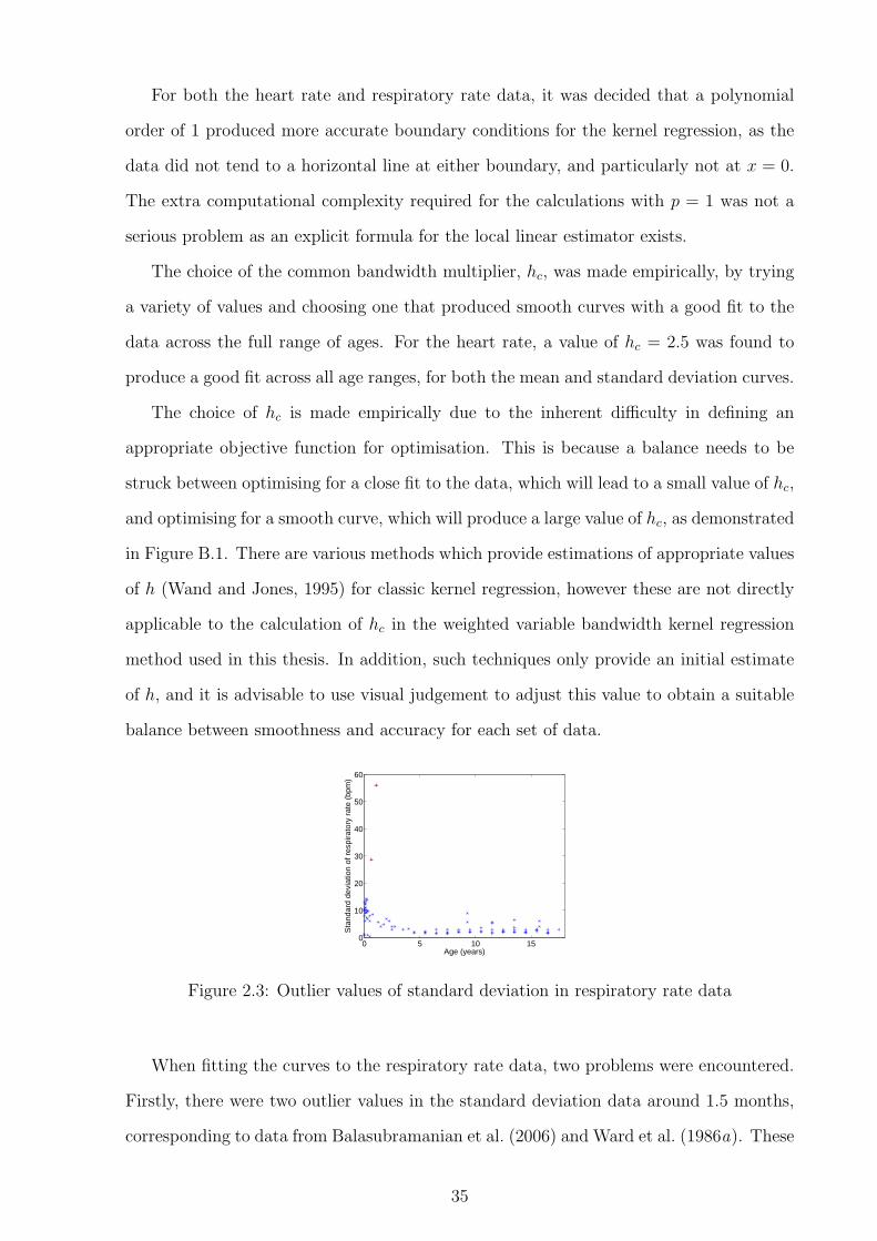
For both the heart rate and respiratory rate data, it was decided that a polynomial

order of 1 produced more accurate boundary conditions for the kernel regression, as the

data did not tend to a horizontal line at either boundary, and particularly not at x = 0.

The extra computational complexity required for the calculations with p = 1 was not a

serious problem as an explicit formula for the local linear estimator exists.

The choice of the common bandwidth multiplier, hc, was made empirically, by trying

a variety of values and choosing one that produced smooth curves with a good fit to the

data across the full range of ages. For the heart rate, a value of hc = 2.5 was found to

produce a good fit across all age ranges, for both the mean and standard deviation curves.

The choice of hc is made empirically due to the inherent difficulty in defining an

appropriate objective function for optimisation. This is because a balance needs to be

struck between optimising for a close fit to the data, which will lead to a small value of hc,

and optimising for a smooth curve, which will produce a large value of hc, as demonstrated

in Figure B.1. There are various methods which provide estimations of appropriate values

of h (Wand and Jones, 1995) for classic kernel regression, however these are not directly

applicable to the calculation of hc in the weighted variable bandwidth kernel regression

method used in this thesis. In addition, such techniques only provide an initial estimate

of h, and it is advisable to use visual judgement to adjust this value to obtain a suitable

balance between smoothness and accuracy for each set of data.

0 5 10 150

10

20

30

40

50

60

Age (years)

Sta

ndar

d de

viat

ion

of r

espi

rato

ry r

ate

(bpm

)

Figure 2.3: Outlier values of standard deviation in respiratory rate data

When fitting the curves to the respiratory rate data, two problems were encountered.

Firstly, there were two outlier values in the standard deviation data around 1.5 months,

corresponding to data from Balasubramanian et al. (2006) and Ward et al. (1986a). These

35

values were considerably larger than the rest of the values in the dataset, and do not fit

in with the overall trend of the data, as can be clearly seen in Figure 2.3. When these

values of standard deviation were used to calculate representative centile data points,

they also resulted in negative respiratory rates, which are not physiologically possible.

For these reasons, these two standard deviation values were excluded from the analysis.

The associated mean values were not excluded, as there was no reason to suspect that

these were also anomalous.

The second problem encountered was that a number of studies reporting data on

respiratory rate in children did so for groups of children spanning very small age ranges.

At the younger end of the age spectrum (under the age of 1 year), almost all of the studies

had very small age ranges, with many studies reporting data for groups of children whose

ages spanned less than one month. This can cause a problem with the variable bandwidth

kernel regression method, as it results in small bandwidths for these data points, meaning

that they have a relatively large local influence on the position of the curve. The sample

sizes of these studies were also typically small, so the number of children in each group was

small, meaning that there could be a large uncertainty in the measurements of respiratory

rate for these groups.

0 5 10 1510

20

30

40

50

60

70

Age (years)

Res

pira

tory

rat

e (b

pm)

datawithout minimum age rangewith minimum age range

(a) Full age range

0 0.5 1 1.5 220

25

30

35

40

45

50

55

60

65

Age (years)

Res

pira

tory

rat

e (b

pm)

datawithout minimum age rangewith minimum age range

(b) Close up of affected area

Figure 2.4: Local influence of data points with small age ranges and solution using mini-mum age range

The large local influence from these studies resulted in the kernel regression estimator

showing that the mean respiratory rate decreases to a local minimum at around 6 months

of age, before rising to a local maximum at around 9 months, and then slowly decreasing

thereafter, as can be seen in Figure 2.4. This does not correspond to existing physiological

36

knowledge, or to the underlying data, and is therefore artefactual. The trough-peak

artefact could be removed by increasing hc, but only to an extent that the rest of the

curve was greatly over-smoothed, and no longer accurately tracked the underlying data

at older ages.

An alternative solution was to set a minimum age range ∆Xmin for the respiratory rate

data. Any data point with an age range below ∆Xmin would have its age range increased

to match this. This allowed us to remove the trough-peak artefact with a minimum of

interference. It was found that a value of ∆Xmin equal to 4 months was sufficient to

remove the artefact in its entirety. Since this was still a small age range for a study, it was

considered that this would be an acceptable modification to the methodology. With this

modification, a value of hc = 1.5 was found to produce a good fit across all age ranges to

both the mean and standard deviation curves for the respiratory rate data.

Subgroup analysis was carried out using one-way ANOVA to test for effects on the

vital signs after correction for age using the method described in Section 2.3. The setting

in which measurements were made, the method of measurement, and the wakefulness of

the child were all tested for their effect on the measured heart rate and respiratory rate.

2.2 Results

The literature search identified 69 studies of interest (Figure 2.2), with 59 studies providing

data on heart rate from 150,080 measurements on 143,346 children, and 20 providing data

on respiratory rate from 7,565 measurements on 3,881 children. Ten studies provided

data on both heart rate and respiratory rate. Included studies had been carried out in

20 different countries across four continents. Summary details of the studies are given in

Tables C.6 and C.7 in Appendix C.

Tables 2.5 and 2.6 show the classification of the included studies on the basis of

study setting, wakefulness, and the method of measurement. The included studies used

a variety of automated methods for measuring respiratory rate, including strain gauges,

thermistors, thoracic impedance, and helium dilution, but there was insufficient data

generated with any one method to merit separate classification.

37

SettingCommunity (e.g. home, school) 27 (39%)Clinical (e.g. hospitals, clinics) 19 (28%)Research laboratories 6 (9%)Unspecified / multiple 17 (25%)

WakefulnessAwake 32 (46%)Asleep 8 (12%)Unspecified / both 29 (42%)

Table 2.5: Classification of settings in which measurements were made, and wakefulnessof children in the included studies in the meta-analysis

Heart rateECG 31 (53%)Automated blood pressure monitor 12 (20%)Manual 6 (10%)Echocardiogram 4 (7%)Other automated method 6 (10%)

Respiratory rateAutomated methods 13 (65%)Manual 7 (35%)

Table 2.6: Classification of the method of measurement in the included studies in themeta-analysis

2.2.1 Heart rate

Figure 2.5 shows the extracted heart rate data, and Figure 2.6 shows the results of the

meta-analysis of heart rate with respect to age in children in terms of the mean and

standard deviation. It can be seen that the heart rate increases from birth to a peak at

around one month of age, and decreases thereafter, with the slope of the curve decreasing

as age increases. The standard deviation remains broadly constant with age, even though

the mean value changes. Tabulated values for the results of the meta-analysis on heart

rate are given in Table D.1 in Appendix D.

The graphs in Figure 2.7 show the peak in heart rate at one month of age in more

detail. Figure 2.7(a) shows the same kernel regression as Figure 2.6, but with the x-axis

limited to only show data up to one year of age, so that the peak at one month can be

more clearly seen. Figure 2.7(b) shows data from the six studies that reported more than

four measurements of heart rate in children under 6 months of age. These show that the

peak in heart rate at around one month of age can be seen in the raw data from multiple

studies, and is therefore not an artefact of the modelling method. Two of the studies,

38

0 2 4 6 8 10 12 14 16 180

20

40

60

80

100

120

140

160

180

200

Age (years)

Hea

rt r

ate

(bea

ts/m

in)

data from individual age groupsmean

Figure 2.5: Heart rate data extracted from 59 papers, and fitted mean

0 2 4 6 8 10 12 14 16 180

20

40

60

80

100

120

140

160

180

200

Age (years)

Hea

rt r

ate

(bpm

)

meanmean +/− 1,2,3 s.d.

Figure 2.6: Meta-analysis of heart rate with respect to age calculated using kernel regres-sion

39

Semizel et al. (2008) and Gemelli et al. (1990), each contributed two lines to the graph in

Figure 2.7(b). This is because these studies reported data separately for male and female

subjects, and so there were two data points for each age group. All of these studies used

automated monitoring equipment (ECG or blood pressure monitors) to measure the heart

rate, making measurement error unlikely.

0 2 4 6 8 10 120

20

40

60

80

100

120

140

160

180

200

Age (months)

Hea

rt r

ate

(bpm

)

meanmean +/− 1,2,3 s.d.

(a) Kernel regression for infants up to one yearof age

0 2 4 6 8 10 12110

120

130

140

150

160

170

Age (months)

Hea

rt r

ate

(bpm

)

betau1980gemelli1990lindner1985semizel2008davignon1980macfarlane1994

(b) Measurements at different ages from singlestudies (note that the scale on the y-axis is ex-panded to allow the peak in heart rate to beclearly seen)

Figure 2.7: Demonstration of peak in heart rate at one month of age

The graphs in Figure 2.8 show the results from the same meta-analysis in the form of a

centile chart showing the mean and representative centiles (1st, 10th, 25th, 75th, 90th and

99th), along with the upper and lower limits from the APLS and PALS guidelines. The

limits shown from the PALS guidelines are those for awake children, since this corresponds

to the more frequent diagnostic situation, as previously discussed.

It can be seen from the graphs that neither guideline corresponds accurately to the

centile charts over all age ranges. The APLS upper limits tend towards the 90th centile

at the lower end of their age ranges, but frequently exceed the 99th centile at the upper

end of the age range, which could result in under-diagnosis of tachycardia (high heart

rate) at certain ages, such as between 3 and 5 years, and 8 and 12 years. The lower limits

follow the 10th centile reasonably well below 2 years of age, but then become too high,

even reaching the value of the mean heart rate at 12 years of age. If these limits are used

40

0 2 4 6 8 10 12 14 16 180

20

40

60

80

100

120

140

160

180

200

Age (years)

Hea

rt r

ate

(bea

ts/m

in)

APLSmeancentiles (1,10,25,75,90,99)

(a) Comparison with APLS limits

0 2 4 6 8 10 12 14 16 180

20

40

60

80

100

120

140

160

180

200

Age (years)

Hea

rt r

ate

(bea

ts/m

in)

PALS (awake)meancentiles (1,10,25,75,90,99)

(b) Comparison with PALS limits for awakechildren

Figure 2.8: Mean heart rate and centiles with respect to age calculated from meta-analysisusing kernel regression and existing limits from APLS and PALS for awake children

in clinical practice, it is very likely that many children will be misclassified as bradycardic

(with excessively slow heart rates), and potentially receive unnecessary investigations or

treatment.

The PALS limits for heart rate are, in general, much wider than those of APLS, and

thus the upper limits exceed the 99th centile for almost the whole age range up to the

age of 10 years. It is therefore probable that these limits would result in under-diagnosis

of tachycardia in children under the age of 10 years. The use of a single lower limit for all

children over the age of 2 years also results in poor performance in predicting bradycardia,

with the limit below the 1st centile for children aged between 2 and 6 years. This is likely

to result in under-diagnosis of bradycardia, particularly in the younger age group, for

whom the distance from the 1st centile is particularly large.

Sub-group analysis of the heart rate data using one-way ANOVA showed that heart

rates measured in community settings were significantly higher (P < 0.0001) than those

measured in clinical or laboratory settings. This may be because studies in community

settings were more likely to involve ambulatory monitoring during normal daily activities,

which might include physical exertion, whereas children measured in clinical or laboratory

settings were likely to be resting, resulting in a lower measured heart rate.

Heart rates measured using automated techniques, such as the ECG, were significantly

41

higher (P = 0.0011) than those measured by manual methods such as palpation or aus-

cultation. This may be due to an increased level of stress in children being monitored by

automated methods. However, as will be seen in the following section, the same effect

was not noted in the respiratory rate data, when stress would be expected to affect both

vital signs in a similar way. An alternative explanation may be that manual methods un-

derestimated the true heart rate due to difficulty in accurately counting the rapid heart

rates found in young children. This phenomenon has been previously reported to account

for underestimation of the heart rate by between 15 and 20 beats/minute in young infants

(Kamlin et al., 2006).

Children measured while awake tended to have higher heart rates than sleeping chil-

dren, although this did not reach statistical significance (P = 0.06).

2.2.2 Respiratory rate

0 2 4 6 8 10 12 14 16 180

10

20

30

40

50

60

70

Age (years)

Res

pira

tory

rat

e (b

eats

/min

)

data from individual age groupsmean

Figure 2.9: Respiratory rate data extracted from 20 papers, and fitted mean

Figure 2.9 shows the respiratory data extracted from the literature, and Figure 2.10

shows the mean and standard deviation results of the meta-analysis for respiratory rate

and age in children. Unlike heart rate, respiratory rate does not show a peak in early

infancy, but declines from birth, with the rate of decrease slowing with age. In contrast

to heart rate, the spread of respiratory rate values around the mean is greater in infancy

and early childhood, reaching a stable level at around 5 years of age. Tabulated values for

42

the results of the meta-analysis on respiratory rate are given in Table D.2 in Appendix D.

0 2 4 6 8 10 12 14 16 180

10

20

30

40

50

60

70

Age (years)

Res

pira

tory

rat

e (b

reat

hs/m

in)

meanmean +/− 1,2,3 s.d.

Figure 2.10: Meta-analysis of respiratory rate with respect to age calculated using kernelregression

The graphs in Figure 2.11 show the meta-analysis for respiratory rate in the form of

a centile chart, with the same representative centiles as were used in the centile charts

for heart rate in Figure 2.8. These graphs are shown with the limits from the APLS and

PALS guidelines superimposed for comparison.

The upper limits for respiratory rate in the APLS guidelines are very low in comparison

to the centile chart for children under 2 years of age, lying mainly between the mean and

the 75th centile, but occasionally even dropping below the mean as far as the 25th centile

for neonates. This could lead to significant over-diagnosis of tachypnoea (fast respiratory

rate) in young children, resulting in unnecessary investigations and treatment. For older

children, the accuracy of the APLS upper limit is variable, but generally lies between the

75th and 99th centiles.

The performance of the lower limit for respiratory rate in APLS is much more worrying.

Between the ages of 3.5 and 5 years, and 8.5 and 10 years, the APLS lower limit lies above

the mean, and it approaches the 75th centile at 5 years and 12 years of age. If this limit

was regularly used in clinical practice, large numbers of children at these ages would be

misdiagnosed with bradypnoea (slow respiratory rate).

The upper limit for the respiratory rate in the PALS guidelines lies above the 99th

43

0 2 4 6 8 10 12 14 16 180

10

20

30

40

50

60

70

Age (years)

Res

pira

tory

rat

e (b

reat

hs/m

in)

APLSmeancentiles (1,10,25,75,90,99)

(a) Comparison with APLS limits

0 2 4 6 8 10 12 14 16 180

10

20

30

40

50

60

70

Age (years)

Res

pira

tory

rat

e (b

reat

hs/m

in)

PALSmeancentiles (1,10,25,75,90,99)

(b) Comparison with PALS limits

Figure 2.11: Mean respiratory rate and centiles with respect to age calculated from meta-analysis using kernel regression and existing limits from APLS and PALS guidelines

centile for much of the age range, potentially resulting in under-diagnosis of children

with clinically relevant tachypnoea. However, at the upper end of the age range, the

PALS upper limit for the respiratory rate begins below the 25th centile, and does not

reach the 75th centile even for 18-year old children, so that older children are likely to be

misdiagnosed as tachypnoeic if PALS upper limits are used in clinical practice.

The PALS lower limits for respiratory rate lie between the 25th and 1st centiles up to

the age of 3 and after the age of 13 years. However, for children between 3 and 6 years,

and between 9 and 13 years, the lower limit as defined by the PALS guidelines is likely to

be too high, and approaches the mean value at 4, 6, and 13 years of age.

Subgroup analysis of the respiratory rate data using one-way ANOVA showed no

effects for study setting (P = 0.09), wakefulness (P = 0.36), or method of measurement

(P = 1.00).

2.3 Proposed age correction method for heart rate

and respiratory rate

The mean and standard deviation curves derived as part of the meta-analysis were used

for age correction of heart rate and respiratory rate prior to data fusion of vital sign

44

data for paediatric triage. For example, to perform age correction for heart rate for a

given child with age x and heart rate y, the kernel regression estimators for heart rate

was interrogated to obtain the mean, µx, and standard deviation, σx, of heart rate at

x. The corrected heart rate yc can then be calculated using the normalisation equation

given in Equation 2.7. Tables of µx and σx for representative ages are given in Appendix

D. For example, when correcting heart rate in a child aged two years, µx = 113.45 and

σx = 14.284.

yc =y − µx

σx

(2.7)

The same procedure was applied to the respiratory rate, where y and yc referred to

the original and corrected respiratory rates, and µx and σx were obtained from the kernel

regression estimators for respiratory rate at age x.

2.3.1 Performance of age correction methods on data from pri-

mary and emergency care

The vital signs datasets described in Appendix A.2 contain measurements of heart rate

and respiratory rate from children in primary and emergency care settings. These datasets

were not used to develop the age correction methods, and so form an appropriate test set

to assess the accuracy of the age correction derived from the literature.

For each measurement in the test set, the kernel regression estimators were used to

find the mean and standard deviation for that age, and then the corrected measurement

was calculated using the normalisation equation.

Performance of heart rate age correction

In assessing the effect of age correction on heart rate, we were able to use the large

FW2 dataset, as almost all of the children in both the FaT and Walsgrave studies had

their heart rates measured. Due to the way these children were recruited (they were

either attending a GP surgery with feverish illness, or had been admitted to a hospital

Paediatric Assessment Unit), they were all experiencing some level of illness, and so would

be expected to show some degree of abnormality in their vital signs. Figure 2.12 shows

45

age correction being applied to the heart rates from this dataset.

0 2 4 6 8 10 12 14 16 1840

60

80

100

120

140

160

180

200

220

240

Age (years)

Hea

rt r

ate

(bpm

)

primary care datameanmean +/− 2 s.d.

(a) Before age correction

0 2 4 6 8 10 12 14 16 18−4

−2

0

2

4

6

8

10

Age (years)

Cor

rect

ed h

eart

rat

e

corrected datameanmedian

(b) After age correction

Figure 2.12: Effect of age correction on heart rate data from the FW2 dataset

The graphs in Figure 2.12 show that the kernel regression estimators derived by the

meta-analysis were able to describe the heart rate data found in the FW2 dataset. It can

be seen that the data in the FW2 dataset had a higher mean value than that predicted by

the meta-analysis, as would be expected given that the population from which the FW2

data was collected consisted of children with suspected infection. These children would

be expected to exhibit varying degrees of tachycardia. However, despite this, the general

trend of the data appears to follow that described by the kernel regression estimators.

The results following age correction using the kernel regression estimators, shown

in Figure 2.12(b), show that the age correction method successfully removed the age

dependence of the heart rate from the data. The units of corrected heart rate on the

y-axis of this graph are standard deviations, as defined by the meta-analysis. So, for

example, a raw heart rate that lies exactly on the predicted mean from the meta-analysis

would transform to a corrected heart rate of zero, and one that lies two standard deviations

below the mean would transform to a corrected heart rate of −2.

Figure 2.13 demonstrates age correction of heart rate on six samples of data from

the FW2 dataset. At six different ages, all children in the FW2 dataset whose age lay

within a six month window (e.g. from 1.75 to 2.25 years) were identified, and normal

46

0 50 100 150 200 2500

0.005

0.01

0.015

0.02

0.025

Heart rate (bpm)

p(x)

1y2y4y6y8y10y

(a) Before age correction

−5 0 5 100

0.05

0.1

0.15

0.2

0.25

0.3

0.35

Corrected heart rate

p(x)

1y2y4y6y8y10y

(b) After age correction

Figure 2.13: Fitted normal distributions on samples of heart rate data at different agesbefore and after age correction of heart rate.

distributions were fitted to their uncorrected and corrected heart rates. The probability

distribution functions of these fitted distributions are plotted in the two graphs in Figure

2.13, which shows that age correction of heart rate causes the distributions of heart rate

at different ages to overlap, as should be the case. The distributions of corrected heart

rate do not completely overlap, with the distributions for older children showing a slightly

reduced corrected mean compared to younger age groups. It is likely that this is because

the severity of illness in the FaT and Walsgrave datasets is greater at younger ages, when

children tend to contract more infections. This would not be the case in the data used

to create the age correction curves, as data were selected to exclude unwell children. The

data used to create the curves would therefore not be expected to reflect the increased

likelihood of infection at younger ages.

The mean of the corrected data was at 1.4 standard deviations, with the median

at 1.3 standard deviations. This disparity was due to the skewing effect of the large

number of children with significant tachycardias, compared to relatively few children with

significant bradycardias. This would be expected clinically, as tachycardia is observed

more frequently than bradycardia, particularly in the presence of infection, which is the

most common diagnosis for the children in the FW2 dataset.

47

Performance of respiratory rate age correction

To assess the effect of age correction on respiratory rate, we used the Walsgrave4 dataset,

as this was the only one that included a measure of respiratory rate. Figure 2.14 shows

age correction being applied to the respiratory rate measurements from the Walsgrave4

dataset.

0 2 4 6 8 10 12 14 16 1810

20

30

40

50

60

70

80

90

100

110

Age (years)

Res

pira

tory

rat

e (b

pm)

primary care datameanmean +/− 2 s.d.

(a) Before age correction

0 2 4 6 8 10 12 14 16 18−5

0

5

10

15

20

25

Age (years)

Cor

rect

ed r

espi

rato

ry r

ate

corrected datameanmedian

(b) After age correction

Figure 2.14: Effect of age correction on respiratory rate data from the W4 dataset

The small size of the dataset, and the quantised nature of the measured respiratory

rates, make it more difficult to assess the performance of age correction on respiratory rate

than on heart rate. However, it can be seen that the majority of the data lies within two

standard deviations of the mean in Figure 2.14(a), with the rest representing tachypnoea,

as would be expected from a dataset collected from children with infections.

If the quantised nature of the data is ignored, it can be seen from Figure 2.14(b) that

much of the age dependency in the data has been removed. As with the heart rate data,

the presence of more abnormally high values resulted in a higher mean corrected value,

at 1.5 standard deviations, than the median corrected value, at 0.95 standard deviations.

48

2.4 Conclusions

This chapter has presented the results of a meta-analysis of heart rate and respiratory

rate variation with age in children. The results of this analysis are used in Chapter 6

to apply age correction to measurements of heart rate and respiratory rate prior to data

fusion.

The centile charts created as part of the meta-analysis have also been compared to

the existing limits published in a variety of guidelines, including APLS and PALS, most

of which appear to be based on clinical judgement. Comparison of the centile charts with

the guidelines in Tables 2.1 and 2.2 showed that none of the existing guidelines conform

well to evidence-based centiles. This discrepancy is likely to lead to under-diagnosis of

abnormal values in some cases, and over-diagnosis in others.

In a clinical setting, the risks associated with under-diagnosis are clear, as children

with abnormal vital signs will not be identified, and so may not receive prompt treatment

or intervention, potentially leading to further deterioration of their clinical condition.

However, over-diagnosing healthy children as having abnormal vital signs can also have a

detrimental effect on the health of the child, as it may lead to inappropriate or unnecessary

investigations or treatment, as well as resulting in excessive usage of healthcare resources.

49

Chapter 3

Measuring respiratory rate using the

finger probe (PPG)

3.1 Introduction

As discussed in Section 1.2.2, existing electronic methods for automated measurement of

respiratory rate are unsuitable for use in the context of paediatric triage, as they tend to

be difficult to apply, and may cause distress to an unwell child. However, as discussed in

Section 1.3, respiratory information is known to be present in the photoplethysmogram

(PPG) waveform derived from a pulse oximeter. This is a less invasive form of monitoring,

which is used routinely in primary and emergency care to monitor heart rate and SpO2,

and so should be an acceptable form of monitoring in a paediatric triage situation. The

addition of accurate respiratory rate estimations to a monitor designed for paediatric

triage would enable such a system to provide added benefit to the clinician, either by

using the age correction method in Section 2.3 to show how abnormal the estimated

respiratory rate is, or by using data fusion methods as described in Chapter 6 to identify

unwell children based on their vital sign measurements.

Breathing information is known to be present in the PPG in two forms. The first form

is referred to in this thesis as “amplitude modulation”, although it is not always exactly

analogous to amplitude modulation as applied in other areas of signal processing such as

broadcasting, where the amplitude (envelope) of a carrier wave is varied in relation to the

information being transmitted. In the context of PPG analysis in this thesis, we will use

50

the terms “amplitude modulation” and “AM” to refer to changes in the level of the PPG

signal, which may include baseline wander as well as variations in the amplitude envelope.

The PPG may also contain breathing information in the variations of the period

between consecutive peaks in the waveform (or other salient points). Since this results

in a variation in the dominant frequency of the PPG signal, it is referred to in this

thesis using the terms “frequency modulation” and “FM”. Again, this is not necessarily

exactly analogous to frequency modulation in other areas such as broadcasting, where the

instantaneous frequency of the signal typically varies with the information being encoded.

3.2 Physiological basis of breathing information in

the PPG

The physiological basis for the breathing information in the PPG is not fully understood.

In this thesis, we consider two types of breathing signal that can be extracted from the

PPG: frequency modulation from variations in heart rate, and amplitude modulation of

the PPG waveform. It is useful to understand the physiological origin of the breathing

signal we are trying to extract, as it allows better understanding of potential failure modes.

3.2.1 Amplitude-modulated breathing signals

The most likely cause of amplitude modulation of the PPG is thought to be pressure

variation in the thorax (chest) and abdomen influencing venous return from the periphery

to the heart, and altering the peripheral blood volume (Lindberg et al., 1992; Dorlas and

Nijboer, 1985; Johansson and Stromberg, 2000). Intrathoracic pressure is low during

inspiration, leading to increased venous return to the heart (Nilsson et al., 2003). It

is believed that respiration-related changes in pressure predominantly affect the venous

system, as venous compliance is much greater than arterial compliance. However, it may

also be possible for arterial transmission of changes in thoracic pressure to occur (Nilsson

et al., 2003). Other possible modulators of the PPG amplitude include respiration-related

changes in the cardiac stroke volume, or the arterial blood pressure (Lindberg et al.,

1992; Foo and Wilson, 2005; Nilsson et al., 2003). These changes are mediated by the

51

sympathetic nervous system, and the vasomotor centre in the brain, which reacts to

stretch receptors in the lung.

Amplitude modulation of the PPG due to changes in intrathoracic pressure is not

likely to be greatly affected by age or health status, as it is not mediated by the nervous

system. However, the strength of the respiratory modulation can be altered by the type

of breathing – primarily thoracic breathing leads to a larger signal as the intrathoracic

pressure has a greater influence on venous return than the intra-abdominal pressure (Jo-

hansson and Stromberg, 2000). The respiratory signal is also influenced by tidal volume

(Nilsson et al., 2003), which affects the pressure in the thorax; and can be reduced in

the presence of significant blood loss (Shelley et al., 2006b), as this reduces the overall

amount of blood present in the circulatory system.

3.2.2 Frequency-modulated breathing signals

Frequency modulation of the heart rate occurs due to a physiological process known as

respiratory sinus arrhythmia (RSA). RSA is mediated by the vagal, or parasympathetic,

nervous system. The beating of the heart is controlled by the sino-atrial (SA) node,

and vagal stimulation of this node resets the cardiac cycle, resulting in a delay before

the next heart beat (Hsieh et al., 2003). Vagal stimualtion is reduced during inspiration

compared with expiration, so the heart rate is decreased during expiration compared with

inspiration.

The nervous impulses that mediate RSA originate primarily from the respiratory and

cardiac centres in the brainstem, but also include contributions from peripheral reflexes

and stretch receptors in the thorax (van Ravenswaaij-Arts et al., 1993). Experiments

on anaesthetised dogs have shown that RSA can increase the uptake of oxygen by 4%

compared to the situation without RSA (Yasuma and Hayano, 2004). It is hypothesised

that this benefit is realised by matching ventilation with perfusion in the lungs, ensur-

ing greater blood flow, and potentially greater gas exchange, during inspiration, while

reducing the cardiac load during expiration, when no significant gas exchange is taking

place. These findings are confirmed by observations made during Cheyne-Stokes respi-

ration, which is a respiratory pattern characterised by periods of apnoea (cessation of

52

breathing) and hyperpnoea (abnormally deep or rapid breathing). It was observed that

heart rate decreased during apnoea, reducing the strain on the heart, and increased during

hyperpnoea, allowing maximum efficiency in gas transport (Yasuma and Hayano, 2004).

The frequency content of heart rate variation (HRV) may be split up into bands.

These include very low frequency (VLF) fluctuations (at frequencies below 0.05 Hz),

which are thought to be related to thermoregulation; low frequency (LF) fluctuations

(around 0.1 Hz) related to baroreflexes; and high frequency (HF) fluctuations due to RSA

at the respiratory rate (e.g. at 0.25 Hz for a person breathing at 15 breaths/minute)

(van Ravenswaaij-Arts et al., 1993). RSA will therefore be affected by conditions that

suppress or enhance HRV. Heart rate variation (and hence RSA) decreases with age, but

can also be reduced by the presence of cardiac and neurological conditions, as well as

some medications such as painkillers and sedatives. Between 5.1 and 7.2 breaths/minute,

RSA tends to entrain the low-frequency baroreflex variation, resulting in a heightened

strength in the RSA component of HRV at these respiratory rates (Lindberg et al., 1992).

As the respiratory rate increases, and moves further away from the baroreflex frequency

of 0.1 Hz (equivalent to 6 breaths/minute), the strength of RSA will tend to decrease (van

Ravenswaaij-Arts et al., 1993).

Traditionally, HRV and RSA have been investigated using the R-R interval calculated

by locating the QRS complexes in the electrocardiogram (ECG). However, recent research

(Bolanos et al., 2006; Lu et al., 2008; Selvaraj et al., 2008) has shown that HRV measures

derived from the PPG (Figure 1.4) can produce results very similar to those from the

ECG (Figure 1.2(b)), indicating that derivation of respiratory information from frequency

modulation of the PPG waveform may be possible.

The strength of RSA tends to decrease with increasing severity of illness. It is therefore

likely to be easiest to extract from ECG or PPG waveforms recorded from young, healthy

people. However, it may still be a useful method to investigate, as long as it is not relied

upon to be present in all patients.

53

3.3 Signal processing for respiratory rate extraction

from the PPG

A literature review was carried out to identify the types of methods used for the extrac-

tion of respiratory rate from amplitude modulation of the PPG waveform and frequency

modulation of the heart rate, prior to assessing these methods in the next chapter.

3.3.1 Extraction of amplitude-modulated signals

There are a large number of papers describing methods for extracting respiratory rate or

breathing waveforms from the amplitude modulation of the PPG. They can be grouped

into five major categories: digital filtering, pulse shape parameters, Fourier transforms,

wavelet analysis, and neural network analysis. Each category is dealt with separately in

the following literature review.

Three papers were identified as describing the use of digital band-pass filtering to ob-

tain a breathing waveform from the PPG. The simplest of these methods is that described

in Nilsson et al. (2005), which uses a 3rd order Butterworth band-pass filter with a pass-

band from 0.1 to 0.3 Hz (6–18 breaths/minute). Breaths in the resulting waveform were

detected manually, and compared to a reference respiratory waveform, with a reported

accuracy of around 95%.

Foo and Wilson (2005) also used digital filtering to obtain a respiratory waveform. In

this case, they claimed to use a non-causal 50th order Wiener filter with zero phase shift,

with the ‘limit’ of the filter set to a bandwidth of 0.1–5 Hz. However, it is not clear how

this filter was derived, as Wiener filters are more usually specified by the additive noise

that is to be removed. It was not possible to replicate the filter from the information

given in this paper.

Nakajima et al. (1996) used a more complex bank of filters to extract a breathing

waveform from the PPG. The analogue signal was first filtered with low- and high-pass

Butterworth filters with cut-offs at 0.1 and 5 Hz. The heart rate signal was then extracted

using a band-pass filter with a pass-band of 1.5–2.3 Hz (90–138 beats/minute), and three

different low pass filters, with cut-off frequencies of 0.3, 0.4, and 0.55Hz (18, 24, and 33

54

breaths/minute) were used to obtain a breathing signal. The choice of low pass filter was

determined by the heart rate, with higher heart rates enforcing a higher cut-off frequency

for the low pass filter. Hysteresis was employed when choosing whether to change filters,

to help prevent too frequent switching of filters. The heart rate and respiratory rate

were determined automatically using zero-crossings and peak detection respectively. A

maximum error of 7 breaths/minute was found for the PPG-derived respiratory rate when

compared with impedance pneumography.

Wendelken et al. (2005) and Mason (2002) described methods for extracting breathing

waveforms from various pulse shape parameters, such as the pulse height, rise time, and

peak amplitude. However, these were unlikely to perform better than an equivalent digital

filter, and so were not considered further.

Wertheim et al. (2009) compared a variety of methods, including low-pass filtering,

amplitude of detected peaks, and Fourier transforms. The reported results were most

promising for the Fourier transform analysis, from which the breathing peak appeared

to have been chosen manually, with an error range from -5.84 to +0.76 breaths/minute

when compared to measurements of respiratory airflow.

Johnston and Mendelson (2004) also applied the fast Fourier transform (FFT) to find

the dominant frequency within the breathing spectrum. This was carried out on three

signals: the raw PPG, the envelope of the peaks of the PPG, and a version that has been

low-pass filtered with a cut-off frequency of 0.7Hz (42 breaths/minute). It was not clear

from the paper how the respiratory frequency was identified from the FFT, or how the

authors chose which pre-processing method to use for calculation of respiratory frequency

at each time point, but the results quoted show errors of up to 6 breaths/minute, with

an average error of around 1–2 breaths/minute.

Shelley et al. (2006a) applied a short-time Fourier transform to a windowed version

of the PPG, and then extracted the respiratory frequency using peak detection in the

range 0.08–0.4 Hz (4.8–24 breaths/minute). When compared to respiratory rates from

measurements of expired carbon dioxide concentrations, most measurements were within

1 breath/minute of the reference, with maximum deviations of around 3 breaths/minute.

A complex method using the continuous wavelet transform (CWT) was described in

55

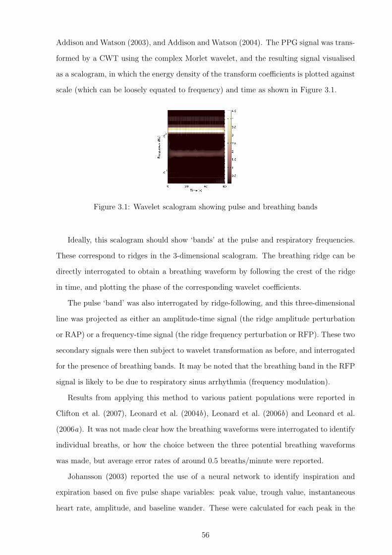
Addison and Watson (2003), and Addison and Watson (2004). The PPG signal was trans-

formed by a CWT using the complex Morlet wavelet, and the resulting signal visualised

as a scalogram, in which the energy density of the transform coefficients is plotted against

scale (which can be loosely equated to frequency) and time as shown in Figure 3.1.

Figure 3.1: Wavelet scalogram showing pulse and breathing bands

Ideally, this scalogram should show ‘bands’ at the pulse and respiratory frequencies.

These correspond to ridges in the 3-dimensional scalogram. The breathing ridge can be

directly interrogated to obtain a breathing waveform by following the crest of the ridge

in time, and plotting the phase of the corresponding wavelet coefficients.

The pulse ‘band’ was also interrogated by ridge-following, and this three-dimensional

line was projected as either an amplitude-time signal (the ridge amplitude perturbation

or RAP) or a frequency-time signal (the ridge frequency perturbation or RFP). These two

secondary signals were then subject to wavelet transformation as before, and interrogated

for the presence of breathing bands. It may be noted that the breathing band in the RFP

signal is likely to be due to respiratory sinus arrhythmia (frequency modulation).

Results from applying this method to various patient populations were reported in

Clifton et al. (2007), Leonard et al. (2004b), Leonard et al. (2006b) and Leonard et al.

(2006a). It was not made clear how the breathing waveforms were interrogated to identify

individual breaths, or how the choice between the three potential breathing waveforms

was made, but average error rates of around 0.5 breaths/minute were reported.

Johansson (2003) reported the use of a neural network to identify inspiration and

expiration based on five pulse shape variables: peak value, trough value, instantaneous

heart rate, amplitude, and baseline wander. These were calculated for each peak in the

56

PPG, and the values for five consecutive heart beats formed the 25 inputs to a neural

network with a single hidden layer containing five neurons, and two outputs. The network

was a fully-connected feed-forward network with sigmoid activation functions. The two

outputs reported whether the inputs follow an inspiration or expiration, and were shown

to give around 95% accuracy when compared to the breaths detected by a humidity

sensor. It was not considered practical to replicate this method, as the training of the

neural network required a gold-standard signal denoting inspiration and expiration. In

the study reported in Johansson (2003), this was provided by creating a square wave from

the output of an airflow humidity sensor, but the quality of the respiratory waveforms

available for this thesis would be likely to result in poor-quality training data, and hence

produce a poorly-trained neural network.

3.3.2 Extraction of frequency-modulated signals

Few papers were found that described the extraction of respiratory rate from frequency

modulation of the PPG due to respiratory sinus arrhythmia (RSA). However, as mentioned

previously, it is known that heart rate variation measured from the PPG is comparable

to that measured from the ECG, and so it is likely that the methods used to extract

respiratory rate from ECG-derived measurements of RSA will be effective when applied

to the PPG.

All of the methods in the literature used a similar pre-processing step to extract a

useful time series from the ECG. This consisted of salient point detection (typically the

R peak of the QRS complex), usually followed by removal/replacement of ectopic beats.

The time series (usually referred to as an R-R time series or tachogram) was constructed

by calculating the time interval between neighbouring salient points, and locating this at

a consistent point in time – usually either the time of the second point, or the mean time

for the two points.

This raw time series is unevenly sampled, and so is not amenable to standard signal

processing techniques without resampling. Resampling was usually carried out by per-

forming cubic spline interpolation on the raw time series, and then resampling this curve

to obtain a regularly sampled signal at the chosen sample frequency. This procedure is

57

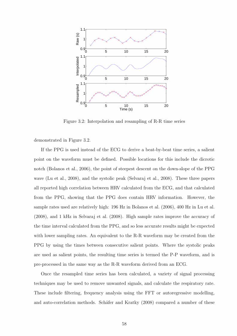
0 5 10 15 200.9

1

1.1

Raw

(s)

0 5 10 15 200.9

1

1.1

Inte

rpol

ated

0 5 10 15 200.9

1

1.1

Res

ampl

ed

Time (s)

Figure 3.2: Interpolation and resampling of R-R time series

demonstrated in Figure 3.2.

If the PPG is used instead of the ECG to derive a beat-by-beat time series, a salient

point on the waveform must be defined. Possible locations for this include the dicrotic

notch (Bolanos et al., 2006), the point of steepest descent on the down-slope of the PPG

wave (Lu et al., 2008), and the systolic peak (Selvaraj et al., 2008). These three papers

all reported high correlation between HRV calculated from the ECG, and that calculated

from the PPG, showing that the PPG does contain HRV information. However, the

sample rates used are relatively high: 196 Hz in Bolanos et al. (2006), 400 Hz in Lu et al.

(2008), and 1 kHz in Selvaraj et al. (2008). High sample rates improve the accuracy of

the time interval calculated from the PPG, and so less accurate results might be expected

with lower sampling rates. An equivalent to the R-R waveform may be created from the

PPG by using the times between consecutive salient points. Where the systolic peaks

are used as salient points, the resulting time series is termed the P-P waveform, and is

pre-processed in the same way as the R-R waveform derived from an ECG.

Once the resampled time series has been calculated, a variety of signal processing

techniques may be used to remove unwanted signals, and calculate the respiratory rate.

These include filtering, frequency analysis using the FFT or autoregressive modelling,

and auto-correlation methods. Schafer and Kratky (2008) compared a number of these

58

methods, most of which had been previously published in German-language publications.

Correa et al. (2008), Cysarz et al. (2008), and Schafer and Kratky (2008) all presented

methods which used filtering to pre-process the time series. Correa et al. (2008) used

a low-pass filter with a cut-off of 5 Hz (equivalent to 300 breaths/minute) to create a

respiratory waveform, but did not calculate a respiratory rate from this, reporting only the

correlation and coherence of the resulting waveform with a number of measured respiratory

waveforms. Cysarz et al. (2008) used a band-pass filter with a pass-band from 0.1–0.45 Hz

(6–27 breaths/minute), and then used peak detection and thresholding to locate breathing

peaks, from which they calculated instantaneous and time-averaged respiratory rates.

These were found to have a mean error of 0.19 breaths/minute, but failed for respiratory

rates of less than 10 breaths/minute or greater than 21 breaths/minute. The method

was also found to be less accurate on older subjects, and during wakefulness. Schafer

and Kratky (2008) described two methods using different types of peak detection on a

waveform following filtering using a 10th order Butterworth band-pass filter with a pass-

band from 0.1–0.5 Hz (6–30 breaths/minute). Their simple method used a threshold to

define ‘valid’ peaks, and produced a respiratory rate with an average error of between 0.014

and 0.033 Hz (0.84–1.98 breaths/minute). A more complex method was also presented

which defined ‘valid’ peaks based on the vertical distance between adjacent maxima and

minima. This slightly improved the estimation of respiratory rate, with an average error

of between 0.014 and 0.03 Hz (0.84–1.8 breaths/minute).

Schafer and Kratky (2008) also reported testing a method using the fast Fourier trans-

form (FFT) to extract a respiratory rate from the time series. This involved finding the

maximum FFT coefficient in the range 0.1–0.5 Hz (6–30 breaths/minute), with heuristics

to determine if this was a valid peak in the spectrum, based on the magnitude and fre-

quency of the next largest coefficient. The accuracy of this method in terms of estimating

a respiratory rate was not reported, but was implied to be lower than that reported for

the filtering methods.

Both Thayer et al. (2002) and Schafer and Kratky (2008) reported the use of meth-

ods using autoregressive (AR) modelling to extract the respiratory rate from an RSA

waveform. Thayer et al. (2002) used an unspecified model to extract the HF frequency

59

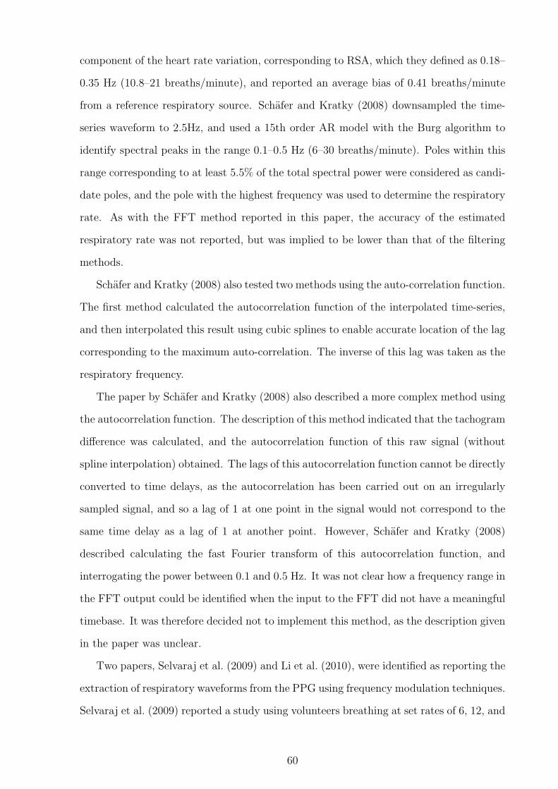
component of the heart rate variation, corresponding to RSA, which they defined as 0.18–

0.35 Hz (10.8–21 breaths/minute), and reported an average bias of 0.41 breaths/minute

from a reference respiratory source. Schafer and Kratky (2008) downsampled the time-

series waveform to 2.5Hz, and used a 15th order AR model with the Burg algorithm to

identify spectral peaks in the range 0.1–0.5 Hz (6–30 breaths/minute). Poles within this

range corresponding to at least 5.5% of the total spectral power were considered as candi-

date poles, and the pole with the highest frequency was used to determine the respiratory

rate. As with the FFT method reported in this paper, the accuracy of the estimated

respiratory rate was not reported, but was implied to be lower than that of the filtering

methods.

Schafer and Kratky (2008) also tested two methods using the auto-correlation function.

The first method calculated the autocorrelation function of the interpolated time-series,

and then interpolated this result using cubic splines to enable accurate location of the lag

corresponding to the maximum auto-correlation. The inverse of this lag was taken as the

respiratory frequency.

The paper by Schafer and Kratky (2008) also described a more complex method using

the autocorrelation function. The description of this method indicated that the tachogram

difference was calculated, and the autocorrelation function of this raw signal (without

spline interpolation) obtained. The lags of this autocorrelation function cannot be directly

converted to time delays, as the autocorrelation has been carried out on an irregularly

sampled signal, and so a lag of 1 at one point in the signal would not correspond to the

same time delay as a lag of 1 at another point. However, Schafer and Kratky (2008)

described calculating the fast Fourier transform of this autocorrelation function, and

interrogating the power between 0.1 and 0.5 Hz. It was not clear how a frequency range in

the FFT output could be identified when the input to the FFT did not have a meaningful

timebase. It was therefore decided not to implement this method, as the description given

in the paper was unclear.

Two papers, Selvaraj et al. (2009) and Li et al. (2010), were identified as reporting the

extraction of respiratory waveforms from the PPG using frequency modulation techniques.

Selvaraj et al. (2009) reported a study using volunteers breathing at set rates of 6, 12, and

60

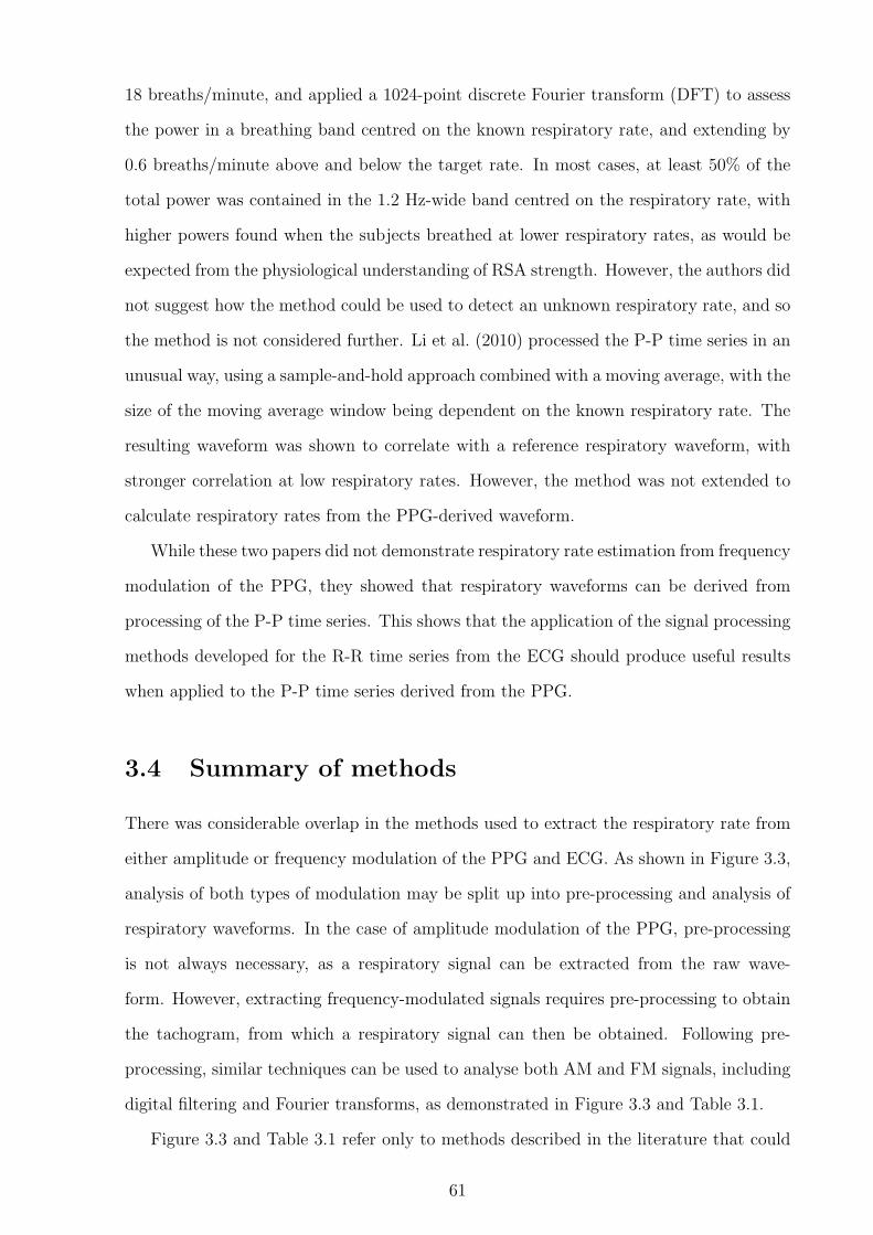
18 breaths/minute, and applied a 1024-point discrete Fourier transform (DFT) to assess

the power in a breathing band centred on the known respiratory rate, and extending by

0.6 breaths/minute above and below the target rate. In most cases, at least 50% of the

total power was contained in the 1.2 Hz-wide band centred on the respiratory rate, with

higher powers found when the subjects breathed at lower respiratory rates, as would be

expected from the physiological understanding of RSA strength. However, the authors did

not suggest how the method could be used to detect an unknown respiratory rate, and so

the method is not considered further. Li et al. (2010) processed the P-P time series in an

unusual way, using a sample-and-hold approach combined with a moving average, with the

size of the moving average window being dependent on the known respiratory rate. The

resulting waveform was shown to correlate with a reference respiratory waveform, with

stronger correlation at low respiratory rates. However, the method was not extended to

calculate respiratory rates from the PPG-derived waveform.

While these two papers did not demonstrate respiratory rate estimation from frequency

modulation of the PPG, they showed that respiratory waveforms can be derived from

processing of the P-P time series. This shows that the application of the signal processing

methods developed for the R-R time series from the ECG should produce useful results

when applied to the P-P time series derived from the PPG.

3.4 Summary of methods

There was considerable overlap in the methods used to extract the respiratory rate from

either amplitude or frequency modulation of the PPG and ECG. As shown in Figure 3.3,

analysis of both types of modulation may be split up into pre-processing and analysis of

respiratory waveforms. In the case of amplitude modulation of the PPG, pre-processing

is not always necessary, as a respiratory signal can be extracted from the raw wave-

form. However, extracting frequency-modulated signals requires pre-processing to obtain

the tachogram, from which a respiratory signal can then be obtained. Following pre-

processing, similar techniques can be used to analyse both AM and FM signals, including

digital filtering and Fourier transforms, as demonstrated in Figure 3.3 and Table 3.1.

Figure 3.3 and Table 3.1 refer only to methods described in the literature that could

61

A

Pre-filter

B

Salient point

detection &

tachogram

creation

A

Pre-filter

C1

Cubic spline

interpolation

C2

Moving

average

M1

Digital filtering

D2

Frequency

detection

D1

Breath

detection

D3

Breath

detection

D4

Pole choice

D5

Lag choice

M2

Fourier

transform

M3

Continuous

wavelet

transform

M4

Autoregressive

modelling

M5

Autocorrelation

function

AM FM

Figure 3.3: Block diagram showing signal analysis methods for obtaining respiratoryrates from AM or FM modulation of the PPG. Blocks above the dashed line correspondto pre-processing steps, whereas blocks below the line correspond to respiratory waveformanalysis.

reasonably be replicated using the datasets available for this thesis. Therefore, techniques

which are not suitable for implementation using this data, or which were not described in

sufficient detail to allow replication, were excluded.

The literature review presented in this chapter shows that it is possible to calculate the

respiratory rate from various properties of the PPG waveform. In the next chapter, the

methods presented in Figure 3.3 are applied to PPG data recorded from adult subjects,

to assess the relative performance of each method. A novel method using auto-regressive

modelling is presented at the end of the chapter.

Although the ultimate aim is to to monitor respiratory rate in children, most of the

methods reported in the literature have only been tested on adults, and many of them

assumed pre-determined limits for the respiratory rates that can be detected. If these

methods were to be applied to data acquired from children, it would be necessary to alter

the limits to allow for the expected range of respiratory rates at the age of the child,

as normal ranges of respiratory rates vary during childhood. This problem is discussed

62

A B C M D

Nilsson et al. (2005) 1 (BPF) 1 (manual)Nakajima et al.(1996)

LPF &HPF

1 (LPF) 1 (manual)

Wertheim et al.(2009)

2 (FFT) 2 (manual)1 (LPF) 1

Johnston andMendelson (2004)

2 (FFT) 2LPF 2 (FFT) 2

Shelley et al. (2006a) 2 (STFT) 2 (auto)Addison and Watson(2003) etc.

3 3 (auto)

Bolanos et al. (2006) dicroticnotch

Lu et al. (2008) EMD max slopeSelvaraj et al. (2008) LPF peak 1 (4Hz)Correa et al. (2008) R peak 1 (100Hz) 1 (LPF)Cysarz et al. (2008) R peak 1 (10Hz) 1 (BPF) 1 (auto)

Schafer and Kratky(2008)

R peak 1 (5Hz) 1 (BPF) 1 (auto)R peak 1 (5Hz) 2 (FFT) 2 (auto)R peak 1 (5Hz) 4 4 (auto)R peak 1 (5Hz) 5 5 (auto)

Selvaraj et al. (2009) peak 1 (4Hz) 2 (DFT)Li et al. (2010) peak 2

Table 3.1: Table showing which blocks are active in each of the methods described inthis chapter. References in italics refer to papers describing methods applied to theECG rather than the PPG waveform. Abbreviations used: LPF (low-pass filter), BPF(band-pass filter), HPF (high-pass filter), EMD (empirical mode decomposition), FFT(fast Fourier transform), STFT (short-time Fourier transform), DFT (discrete Fouriertransform). Where possible, the final column denotes whether detection was carried outmanually or automatically. Each column in this table corresponds to an analysis stageas shown in Figure 3.3. Numbers in the table refer to the specific block that is used in agiven method; e.g. a ‘2’ in column M refers to block M2 (Fourier transform) in the blockdiagram.

further in Chapter 5.

63

Chapter 4

Accuracy of respiratory rate

estimation in adults

4.1 Introduction

The eventual aim of the work described in Chapters 3, 4, and 5 is to estimate respiratory

rate in a minimally invasive way in children, ideally using the PPG waveform from a pulse

oximeter finger probe. The lack of paediatric photoplethysmogram data meant that the

signal processing methods could not be evaluated on data acquired from children until we

collected such data ourselves The initial algorithm development and testing was therefore

carried out using data from adult subjects, with the aim of adapting the best-performing

algorithms for use with paediatric data.

The data used for these investigations came from the MIMIC and Controlled Breathing

databases described in Appendix A, which both contain synchronous measurements of the

PPG and a reference breathing waveform.

Potential methods for the estimation of respiratory rate from the PPG were identified

from the literature reviewed in Chapter 3. As seen in Figure 3.3, five classes of method

were identified for analysing the waveforms derived from either amplitude or frequency

modulation of the PPG. A number of these classes were observed as having been applied

to both amplitude and frequency modulation, which is not surprising given that both

problems can be viewed as obtaining a respiratory rate from a signal incorporating a

breathing-synchronous waveform. This waveform may be derived from the AM variation,

64

with or without pre-filtering, or it may result from the calculation of a tachogram, allowing

analysis of FM variations in the signal. It was therefore decided that, where possible,

all methods would be assessed in the AM domain, in which there is greater evidence

for applying methods to the PPG signal, and that the best-performing method in this

domain would then be tested in the FM domain. In the case of the autocorrelation

function (method M5 in Figure 3.3), analysis was confined to the FM domain, as the

method assumes that there is no frequency content due to the heart rate, which is not

the case in the AM domain.

4.2 Testing procedure

The testing procedure was designed so that, as far as possible, the different methods could

be directly compared. To this end, the data was pre-processed before the start of the tests,

so that the input data to the different algorithms would be identical. Algorithms were

tested using the data from both the MIMIC and Controlled Breathing databases.

4.2.1 Windowing of data

The intended goal of this research is to provide real-time monitoring of patients, and

so data was windowed prior to being presented to the algorithms. For each database,

both 30-second and 60-second windows were tested in the AM tests, with 60-second and

120-second windows being used for the FM analysis. Longer windows were used for the

FM analysis as initial investigations showed that FM analysis with 30-second windows

produced estimated respiratory rates with much larger levels of error. This was thought

to be due to problems with the generation of the initial tachogram. As the tachogram

was generated from the time interval between salient points, small errors in the location

of these salient points may have a large effect on the tachogram. Since the peaks in

the PPG waveform are less well defined than the QRS complex in the ECG waveform,

determining the exact location of these peaks is challenging. In addition, changes in the

P-P time due to artefacts such as incorrectly identified or missed peaks, or ectopic heart

beats1 will cause large deviations in the tachogram. Errors introduced during generation

1Ectopic beats are extra or dropped heart beats that result in an irregular instantaneous heart rate.

65

of the tachogram have a greater effect on the estimated respiratory rate when the window

is small, as they make up a larger proportion of the information in the window.

In all cases, consecutive windows were defined to be separated by 5 seconds, to provide

a large degree of overlap between consecutive windows (e.g. 55 seconds of overlap for

consecutive 60-second windows).

Longer windows will generally produce more accurate results, as they contain more

breathing cycles, allowing the effects of short-term artefacts or poor signal quality to be

mitigated. However, this increased accuracy is at the expense of increased delay, both in

terms of the initial delay from the start of recording to the time of the first measurement

(one window length), and in terms of the delay in tracking a changing respiratory rate.

The window length does not affect the frequency of measurements, as this is determined

solely by the delay between successive windows. In this case, a 5-second delay will result

in 12 measurements each minute (0.2 Hz).

4.2.2 Quality metric

The accuracies of the different methods were compared using the absolute error in res-

piratory rate. Execution time was monitored, as the aim of this thesis is to produce a

method which can be used for real-time monitoring, and so a method which does not run

in real time is of no practical use. The execution times are not directly reported, unless

they were so slow that the method would not allow for real-time monitoring.

To calculate the respiratory rate error, the reference respiratory waveform was subject

to pre-processing and breath detection as described in Appendices A.1.1 and A.1.2. The

ensemble average respiratory rate from the reference breathing waveform was calculated

for each window, and the absolute difference between this and the reported respiratory

rate from the method under test was stored as the error for that window.

For comparison of the methods, a number of summary statistics were calculated for

each of the four combinations of data source and window length. Both the mean error,

and the 5% and 95% percentiles were calculated, to give an indication of the spread of

error values. The failure mode of each method was also investigated, as a method with

a failure mode that can be detected is of more use than one which produces errors that

66

cannot be distinguished from a true result.

4.3 Measuring breathing from the amplitude modu-

lation of the PPG

Figure 3.3 in the previous chapter identified five classes of methods which can be used to

analyse the waveforms from AM and FM pre-processing of the PPG signal. Of these five,

four were suitable for investigation in the AM domain: digital filtering, Fourier transforms,

continuous wavelet transforms, and autoregressive modelling. The fifth, autocorrelation

functions, assumes that the highest frequency present in the signal is due to the respiratory

rate, which is not the case in AM-preprocessed signals, as even pre-filtering would be

unlikely to remove all traces of the frequencies corresponding to the heart rate. This

method is therefore investigated further in Section 4.4.

Autoregressive modelling was identified as a possible method for analysing frequency-

modulated respiratory waveforms in Schafer and Kratky (2008). However, our work on an

autoregressive modelling technique for the analysis of amplitude-modulated PPG signals

pre-dates this paper (Fleming and Tarassenko, 2007), and is presented in this chapter.

4.3.1 Digital filtering

Table 3.1 shows that six papers used digital filtering techniques for AM or FM analysis of a

PPG- or ECG-derived signal (Nilsson et al., 2005; Nakajima et al., 1996; Wertheim et al.,

2009; Correa et al., 2008; Cysarz et al., 2008; Schafer and Kratky, 2008). This section

compares the performance of four of these methods; the method described in Wertheim

et al. (2009) is not considered as the paper contained insufficient information to replicate

the filters, and the method described in Correa et al. (2008) is applicable only to FM

data, as the cut-off frequency does not remove frequencies due to the heart rate, which

are present in AM-derived signals.

Table 4.1 describes the design of the filters used in the four methods under investiga-

tion. As can be seen from the table, the method proposed by Nakajima et al. (1996) used

five filters: two pre-filters, and three respiratory extraction filters. The choice between

67

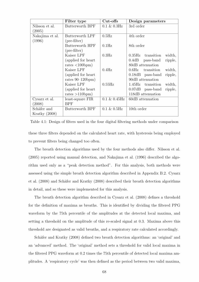
Filter type Cut-offs Design parametersNilsson et al.(2005)

Butterworth BPF 0.1 & 0.3Hz 3rd order

Nakajima et al.(1996)

Butterworth LPF(pre-filter)

0.5Hz 4th order

Butterworth HPF(pre-filter)

0.1Hz 8th order

Kaiser LPF(applied for heartrates <100bpm)

0.3Hz 0.35Hz transition width,0.4dB pass-band ripple,80dB attenuation

Kaiser LPF(applied for heartrates 90–120bpm)

0.4Hz 0.6Hz transition width,0.18dB pass-band ripple,90dB attenuation

Kaiser LPF(applied for heartrates >110bpm)

0.55Hz 1.45Hz transition width,0.07dB pass-band ripple,118dB attenuation

Cysarz et al.(2008)

least-square FIRBPF

0.1 & 0.45Hz 60dB attenuation

Schafer andKratky (2008)

Butterworth BPF 0.1 & 0.5Hz 10th order

Table 4.1: Design of filters used in the four digital filtering methods under comparison

these three filters depended on the calculated heart rate, with hysteresis being employed

to prevent filters being changed too often.

The breath detection algorithms used by the four methods also differ. Nilsson et al.

(2005) reported using manual detection, and Nakajima et al. (1996) described the algo-

rithm used only as a “peak detection method”. For this analysis, both methods were

assessed using the simple breath detection algorithm described in Appendix B.2. Cysarz

et al. (2008) and Schafer and Kratky (2008) described their breath detection algorithms

in detail, and so these were implemented for this analysis.

The breath detection algorithm described in Cysarz et al. (2008) defines a threshold

for the definition of maxima as breaths. This is identified by dividing the filtered PPG

waveform by the 75th percentile of the amplitudes at the detected local maxima, and

setting a threshold on the amplitude of this re-scaled signal at 0.3. Maxima above this

threshold are designated as valid breaths, and a respiratory rate calculated accordingly.

Schafer and Kratky (2008) defined two breath detection algorithms: an ‘original’ and

an ‘advanced’ method. The ‘original’ method sets a threshold for valid local maxima in

the filtered PPG waveform at 0.2 times the 75th percentile of detected local maxima am-

plitudes. A ‘respiratory cycle’ was then defined as the period between two valid maxima,

68

when there is only a single detected local minimum between these (i.e. there are no invalid

maxima in the interval between the valid maxima). The ‘advanced’ method calculates

the difference in amplitude between subsequent extrema (maxima and minima), and then

sets a threshold of 0.3 times the 75th percentile of these differences. Pairs of extrema

are removed until all of the remaining differences are greater than this threshold, and the

periods between each of the remaining maxima determine the length of the respiratory

cycles. The respiratory frequency was defined as the reciprocal of the mean respiratory

cycle length, and the respiratory rate in breaths/minute can be calculated as 60 times the

respiratory frequency.

30 s window 60 s windowMIMIC CB MIMIC CB

Nilsson et al. (2005) 0.84 4.19 0.43 3.71(0.05–2.46) (0.14–12.8) (0.02–1.29) (0.09–12.2)

Nakajima et al. (1996) 1.60 4.14 1.22 3.70(0.03–5.05) (0.18–11.1) (0.01–4.16) (0.15–9.69)

Cysarz et al. (2008) 6.38 5.42 7.37 4.72(0.02–14.2) (0.19–15.7) (0.01–15.2) (0.14–14.2)

Schafer and Kratky (2008) 1.88 3.98 1.58 3.44(original method) (0.05–6.02) (0.18–11.2) (0.03–5.62) (0.12–11.0)Schafer and Kratky (2008) 1.61 4.04 0.99 3.85(advanced method) (0.03–4.60) (0.19–11.1) (0.01–3.40) (0.15–11.9)

Table 4.2: Results from tests on digital filtering methods. Values show are mean (5th–95thpercentile) absolute errors in the respiratory rate in breaths/minute.

The results of applying these algorithms to the MIMIC and Controlled Breathing

(CB) databases are shown in Table 4.2. These results show that the PPG signals from

the Controlled Breathing database tended to produce much less accurate results than

those from the MIMIC database. This could be partly due to the remaining baseline

variation in the signals from the Controlled Breathing database, as discussed in Section

A.1.2. Error rates were generally lower when 60-second windows were used, in comparison

to 30-second windows. This was expected, as longer windows contain more respiratory

cycles, and so more information was available when calculating the average respiratory

rate.

Overall, the method proposed by Nilsson et al. (2005) appeared to perform best, de-

spite the fact that this method used the simplest filtering regime. Figure 4.1 demonstrates

69

0 10 20 30 40 50 60−0.5

0

0.5

PP

G

0 10 20 30 40 50 60−0.1

0

0.1

Filt

ered

0 10 20 30 40 50 60

−0.5

0

0.5

Ref

eren

ceTime (s)

Figure 4.1: Comparison of PPG-derived waveform from digital filtering using the methodproposed by Nilsson et al. (2005) and the reference respiratory waveform, with detectedbreaths marked in black.

the operation of this method on data from the MIMIC database and Figure 4.2 shows

examples of the estimated respiratory rates for patients from the two databases. These

two patients are used as examples for all the methods investigated in this chapter.

0 500 1000 1500 200010

12

14

16

18

20

Time (s)

Bre

athi

ng r

ate

(bre

aths

/min

ute)

Patient 401

Reference

Nilsson

(a) MIMIC patient 401

0 500 1000 1500 2000 2500 30000

5

10

15

20

25

Time (s)

Bre

athi

ng r

ate

(bre

aths

/min

ute)

Patient 3006

Reference

Nilsson

(b) Controlled Breathing patient 3006

Figure 4.2: Reference respiratory rates and rates calculated using the method proposedby Nilsson et al. (2005) for selected patients from the MIMIC and Controlled Breathingdatabases, using 60-second windows.

The graphs in Figure 4.2 show that the algorithm proposed by Nilsson et al. (2005)

was very accurate on the MIMIC data, but consistently failed to detect high respiratory

rates in the data from the Controlled Breathing database, although it was reasonably

accurate at low and intermediate respiratory rates for this database. It is particularly

worrying that the failure mode of this method resulted in reported respiratory rates that

lay in the normal breathing range, as shown in Figure 4.2(b), so that a failure of this

method would not lead to an alarm condition and human intervention.

70

4.3.2 Fourier transforms

Table 3.1 shows that five different papers reported the use of Fourier transforms to esti-

mate the respiratory rate from AM or FM modulation of a PPG or ECG waveform. Three

papers (Wertheim et al., 2009; Johnston and Mendelson, 2004; Schafer and Kratky, 2008)

reported using the fast Fourier transform (FFT), and one (Selvaraj et al., 2009) reported

using the discrete Fourier transform (DFT). As the FFT is a particular algorithm for cal-

culating the DFT, these two methods may be considered equivalent. Shelley et al. (2006a)

described a method using the short-time Fourier transform (STFT), which is equivalent

to performing an FFT analysis on windows of data from the original signal. Since this

method was effectively replicated by applying an FFT method to each window of data,

as described earlier in this section, the STFT method was not considered to be different

to an equivalent FFT method.

With the exception of Johnston and Mendelson (2004), all of the above papers de-

scribed the application of a Fourier transform method to the raw signal, without pre-

filtering. Johnston and Mendelson (2004) applied the method to three signals: the raw

PPG, the envelope of the peaks of the PPG, and a version that had been low-pass filtered

with a cut-off frequency of 0.7Hz (42 breaths/minute). The paper did not describe how

to select the optimum method for each section of data, and so the choice of method was

made by comparing the absolute errors in the respiratory rate for each method, with the

best-performing method being chosen as the predicting method for that section. Where

multiple methods produced the same error in respiratory rate, the least computationally

intensive method was chosen. This allowed the best possible performance to be assessed.

Since this method would always equal or exceed the performance of the methods which

used only the raw signal as an input, only the method described by Johnston and Mendel-

son (2004) was examined in this section. Although Johnston and Mendelson (2004) did

not describe windowing the data, this is a standard step in FFT analysis, and so a Han-

ning window was applied to each section of data immediately prior to computation of the

FFT.

Information on the interpolation of the peak envelopes was not given in the paper,

so cubic splines were used to give a continuous waveform. In a similar way, the only

71

0 10 20 30 40 50 60−1

−0.5

0

0.5

1

Time (s)

Raw

Envelope

Filtered

(a) PPG-derived waveforms

10 20 30 400

0.02

0.04

Raw

10 20 30 400

0.02

0.04

Env

elop

e

10 20 30 400

0.02

0.04

Filt

ered

Breathing rate (breaths/minute)

(b) FFT spectra

Figure 4.3: PPG-derived waveforms and corresponding FFT frequency spectra for thethree methods proposed by Johnston and Mendelson (2004).

information on the low-pass filter was the cut-off frequency, so a number of Butterworth

filters of different orders were tested, with the results compared visually against the sample

published waveform. This resulted in the choice of a 7th order filter.

0 500 1000 15000

5

10

15

20

25

30

Time (s)

Bre

athi

ng r

ate

(bre

aths

/min

ute)

Patient 401

Reference

FFT

(a) MIMIC patient 401

0 500 1000 1500 2000 2500 30000

5

10

15

20

25

Time (s)

Bre

athi

ng r

ate

(bre

aths

/min

ute)

Patient 3006

Reference

FFT

(b) Controlled Breathing patient 3006

Figure 4.4: Reference respiratory rates and rates calculated using the method proposedby Johnston and Mendelson (2004) for reference patients from the MIMIC and ControlledBreathing databases, using 60-second windows.

Figure 4.3(b) shows the spectra obtained from the three PPG-derived waveforms. The

frequency of the spectral component with the highest amplitude in the region correspond-

ing to respiratory rates between 3 and 42 breaths/minute was taken as the respiratory

frequency.

The results of applying this method to the data in the MIMIC and Controlled Breath-

ing databases are shown in Table 4.3. This shows that 30-second windows produced more

accurate estimates of respiratory rate than 60-second windows when FFT methods were

72

30 s window 60 s windowMIMIC CB MIMIC CB

Mean error 0.72 6.59 0.75 7.165-95% errors 0.05–4.48 0.13–16.0 0.06–4.77 0.09–16.7Raw PPG (%) 96.0 89.1 96.9 88.5Peak envelope (%) 3.32 8.19 2.52 9.28Low-pass filtered (%) 0.68 2.67 0.57 2.21

Table 4.3: Results from test using Fourier transform methods. Mean and 5th–95th per-centile errors are calculated from absolute errors in respiratory rate in breaths/minute.The percentage of the windows for which each of the three potential source waveformsare used to obtain the most accurate estimate of respiratory rate are shown in the lowerpart of the table. Note that columns do not sum to exactly 100% due to rounding.

employed. This appears counter-intuitive, as the smaller window contained less data,

and so there was correspondingly lower resolution in the frequency domain of the FFT.

However, it is possible that the lower frequency resolution reduced the ability of the FFT

to detect low frequency variations in the PPG waveform. This would correspond the the

observed failure mode of the FFT method seen in Figure 4.4, where the algorithm chooses

the lowest frequency in the range of interest. This may be due to residual baseline wander

in the PPG waveform, which would explain why the accuracy is lower for data from the

Controlled Breathing database, which has higher levels of baseline wander that the data

in the MIMIC database.

It might be possible to improve the accuracy by looking for a true peak (i.e. one

with lower values on each side), rather than simply the highest value in the spectrum,

although this method was not reported in any of the papers discussed in Chapter 3. Even

if this method was implemented, it is unlikely that it would improve the performance of

FFT respiratory rate estimation on the high respiratory rate sections of the data from the

Controlled Breathing database, where the FFT method consistently failed to choose the

correct value, even where it did not choose the lowest frequency in the range of interest.

It is possible that this issue was an artefact of the way in which the Controlled Breathing

database was collected. The subjects were attempting to breathe at a predetermined rate,

and were not breathing regularly, as demonstrated in Figure 4.21. Such irregularities in

the instantaneous respiratory rate would spread out the spectral peak and make it less

easy to identify. This hypothesis is supported by results from the MIMIC database, where

73

the FFT method was able to detect the correct rate in patients who showed equally high

respiratory rates as those in the Controlled Breathing database, but were breathing either

spontaneously or with the assistance of a ventilator.

Table 4.3 also shows that the raw PPG was identified as the best-performing method

in over 80% of cases, implying that further processing to obtain the peak envelope or

filtered signal may not significantly improve the respiratory rate estimation.

4.3.3 Continuous wavelet transforms

Leonard et al. (2006a,b, 2004a,b, 2003); Clifton et al. (2007); and Addison and Watson

(2004, 2003) used continuous wavelet transforms to extract a breathing waveform from the

PPG. The continuous wavelet transform allows for arbitrary frequency resolution, unlike

the more frequently applied discrete wavelet transform. The complex Morlet wavelet was

used for the transform, and the resulting signal was visualised as a scalogram, where the

energy density function of the transform coefficients, |T (a, b)|2, is plotted against scale

(which can be loosely equated to frequency) and time.

(a) Wavelet scalogram

0 10 20 30 40 50 60−5

0

5

Bre

athi

ng b

and

0 10 20 30 40 50 60−1

−0.5

0

0.5

1

Time (s)

Ref

eren

ce

(b) Breath detection from breathing band

Figure 4.5: Wavelet scalogram showing pulse and breathing bands, and detection ofbreaths (marked with black stars) from the phase of the wavelet coefficients in the breath-ing band.

Figure 4.5(a) shows the scalogram for part of one of the MIMIC PPG signals, in which

a breathing band is visible at around 0.34 (10−0.5) Hz, corresponding to a respiratory rate

of 20.4 breaths/minute. This band represents a ridge in the 3-dimensional scalogram, and

74

can be directly interrogated to obtain a breathing waveform by following the crest of the

ridge in time, and plotting the phase of the corresponding wavelet coefficients, as shown

in Figure 4.5(b).

Although the example in Figure 4.5 has a clearly identifiable breathing band, this was

not always the case, and so further analysis was carried out on the band corresponding to

the heart rate, which can be seen in the scalogram as a high ridge at around 1.4 (100.16) Hz

(84 beats/minute). This secondary analysis was carried out in every case, as even when

a breathing band was present, information from the heart rate band may contain more

accurate breathing information. The crest of this ridge was also followed, and projected

as both an amplitude-time and a frequency-time signal. These two signals are referred

to as the ridge amplitude perturbation (RAP) and ridge frequency perturbation (RFP)

respectively.

The papers did not give any detail as to the nature of the ridge following algorithm,

so the following algorithm was devised. For the purpose of this algorithm, it is assumed

that the three dimensions are time (x-axis), position (y-axis) and height (z-axis). For any

given point in time, there will be exactly one point on the locus of the ridge. The ridge

was also assumed to be broadly continuous, so that large changes in y were penalised.

An initial estimate of the position of the ridge was calculated by identifying the max-

imum in the sum over time for the heights at each position. The flanking local minima

defined the limits of the search space. For each time point in the scalogram, the ridge

position was determined by looking for the point of maximum height for a region around

the last position. The size of this region was dependent on the height of the last position,

so that noise did not dominate if the ridge was ill-defined.

The two secondary signals from ridge following in the pulse (heart rate) band were

then subjected to wavelet transformation in the same way as the initial signal. This

is referred to as secondary waveform feature decoupling (SWFD). The RAP and RFP

signals and their associated scalograms are shown in Figures 4.6 and 4.7. The scalograms

in these figures were rescaled by dividing by the wavelet scale, (|T (a, b)|2)/a, in order to

emphasise the ridges.

The RAP and RFP scalograms were interrogated to find a breathing ridge, from

75

0 10 20 30 40 50 601

2

3

4

5

6

Time (s)

Sca

logr

am a

mpl

itude

(a) RAP signal from pulse band (b) RAP wavelet scalogram with breath-ing band

Figure 4.6: RAP signal and scalogram

0 10 20 30 40 50 601.4

1.45

1.5

1.55

1.6

Time (s)

Fre

quen

cy (

Hz)

(a) RFP signal from pulse band (b) RFP wavelet scalogram

Figure 4.7: RFP signal and scalogram

which a breathing waveform was obtained in the same way as for the breathing ridge

in the original scalogram. In Figure 4.6, a faint breathing band is visible, and produces

a reasonably accurate breathing signal, but the RFP does not contain a band at the

respiratory frequency (Figure 4.7). This was not particularly surprising, as it is likely

that the RFP scalogram corresponds to heart rate variability, which is known to be low

in the MIMIC patients, who were all severely unwell. Figures 4.5–4.7 were all obtained

from data from a single MIMIC patient.

The main difficulty with this method was the requirement to perform continuous

wavelet transforms at low frequencies. At the low frequencies associated with breathing,

the wavelet is scaled to have a long duration. This led to many large and computationally

intensive convolution operations to form the scalogram.

In the initial implementation, the first scalogram (on the raw PPG signal), was cal-

76

culated for 200 scales spaced logarithmically between 0.05 and 5 Hz (3-300 bpm). This

allowed for reliable identification of the pulse and breathing bands, and allowed tracking

of the breathing band ridge, but did not generally produce sufficient frequency resolu-

tion in the pulse band to obtain the RFP. Therefore the pulse band was identified, and

then the original PPG waveform was wavelet-transformed within this band only. Since

the pulse band is at a higher frequency than the breathing band, it did not require such

computationally expensive convolutions, and so this step did not significantly increase the

computational complexity. The high-resolution scalogram was calculated with 200 times

the number of scales identified in the pulse band of the low-resolution scalogram. The

scalograms for the RAP and RFP signals were calculated for 200 scales logarithmically

spaced between 0.05 and 1 Hz (3-60 breaths/minute). There were therefore three scalo-

grams that needed to be calculated at low frequencies: the original PPG scalogram, the

RAP scalogram, and the RFP scalogram. The scalograms and traces shown in Figures

4.5–4.7 were all created using this initial implementation of the method.

As this method was so slow that it was unlikely to be of any practical use, an attempt

was made to speed it up by reducing the number of scales used in these three scalograms.

The number of scales was reduced by a factor of 10, so that only 20 logarithmically spaced

scales were calculated for the three low-frequency scalograms. This increased the speed

by a factor of 6, but the algorithm was still at least 6 times slower than the real-time

benchmark (i.e. 1 hour of data took at least 6 hours to process).

To allow for comparison between the two methods, both were run on the two datasets,

with results as shown in Table 4.4. To obtain a robust measurement of respiratory rate,

Leonard et al. (2006b) suggested that information from all three sources (the initial trans-

form, the RAP and the RFP) could be compared to determine the optimal signal to use

in each situation. For the results presented in this report, the ‘best’ method for each

test PPG was selected as the method that produced the lowest error in respiratory rate

estimation. This would not be possible in practice, but allowed the best possible results

to be used for comparison.

Table 4.5 shows how often each of the various breathing band sources were used to

calculate the respiratory rate. This shows that the optimal source was fairly evenly split

77

30 s window 60 s windowMIMIC CB MIMIC CB

Original method 1.55 3.99 1.30 3.55(0.07–4.76) (0.18–12.5) (0.04–3.79) (0.13–11.6)

Faster method 3.33 5.16 2.60 4.63(0.26–8.9) (0.27–14.6) (0.18–9.6) (0.19–13.5)

Table 4.4: Results from continuous wavelet transform analysis of the PPG. Mean (5–95%percentile) absolute errors in respiratory rate are shown in breaths/minute

between the three possibilities, so it would almost certainly be necessary to calculate all

three and develop an algorithm to choose the best option without a priori knowledge of

the true respiratory rate. This would add an extra level of complexity to a method that

is already very computationally expensive.

Source 30 s window 60 s windowMIMIC CB MIMIC CB

Original Raw PPG (%) 39.0 33.8 40.9 29.9method RAP (%) 29.2 38.5 30.9 33.8

RFP (%) 31.8 27.7 28.2 36.3Faster Raw PPG (%) 10.3 33.9 37.2 28.4method RAP (%) 36.6 37.2 34.0 23.5

RFP (%) 53.1 28.9 28.8 48.2

Table 4.5: Frequency of use of the three different scalogram breathing bands in estimatingrespiratory rate using the continuous wavelet method. Note that columns do not sum toexactly 100% due to rounding.

As neither method was capable of real time analysis, they are not suitable for patient

monitoring in their current form. As can be seen in Figure 4.8, the wavelet methods also

failed in the same way as the digital filtering methods, with low accuracy at the high

respiratory rates seen in the CB database. The failure mode again led to the respiratory

rate being incorrectly estimated to lie within the normal range.

4.3.4 Autoregressive modelling

Autoregressive (AR) modelling has been applied to a number of physiological signals,

including the EEG (Pardey et al., 1996) and the intrapartum cardiotocogram (Cazares

et al., 2001). The technique described was developed prior to the publication of the paper

by Schafer and Kratky (2008). It uses autoregressive modelling for the extraction of

78

0 500 1000 15000

5

10

15

20

25

Time (s)

Bre

athi

ng r

ate

(bre

aths

/min

ute)

Patient 401

ReferenceSlow waveletsFast wavelets

(a) MIMIC patient 401

0 500 1000 1500 2000 2500 30000

5

10

15

20

25

Time (s)

Bre

athi

ng r

ate

(bre

aths

/min

ute)

Patient 3006

Reference

Slow wavelets

Fast wavelets

(b) Controlled Breathing patient 3006

Figure 4.8: Reference respiratory rates and rates calculated using the method proposedby Addison and Watson (2003) for selected patients from the MIMIC and ControlledBreathing databases, using 60-second windows.

respiratory rate from the photoplethysmogram (Fleming and Tarassenko, 2007).

The mathematical background to AR modelling is described in Section B.3. It was

hypothesised that the pole in an AR model of the PPG signal corresponding to the

respiratory rate could be identified from a search of the poles with phase angles within a

range defined by the expected respiratory frequencies for a normal subject.

The signal was first pre-filtered to reduce the magnitude of spectral components due

to the heart rate, as these would tend to dominate the spectrum and so decrease the

placement accuracy of the breathing pole. The filter used for this purpose was a low-pass

filter designed using the Kaiser windowing function, with a transition band from 0.4–0.8

Hz (24–48 breaths/minute), 5% ripple in the pass-band, and 30 dB of attenuation in the

stop-band.

It was also necessary to downsample the signal prior to AR modelling. The PPG signal

was typically sampled at between 100 and 250 Hz to ensure that the shape and heart rate

information are preserved. At such high sample rates, the AR phase angles corresponding

to respiratory frequencies were very small, which was likely to lead to inaccuracy in

identifying the breathing pole, or possibly even the absence of a breathing pole in the

AR model (since it would be subsumed into the real-axis, or d.c., poles). Downsampling

increased the angular resolution of low frequency information, and also further reduced

the influence of the cardiac-synchronous pulsatile component of the PPG. A decimation

algorithm, which filters the signal prior to resampling, was used to reduce the effect of

79

aliasing in the downsampled signal. The downsampled PPG was then detrended to remove

any DC offset, which improved the stability of the AR model. The poles of the AR model

were then calculated using the Yule-Walker method. This method was chosen after initial

investigations showed that the estimated respiratory rate was more accurate when poles

were calculated using the Yule-Walker method, compared with the Burg method.

For models with an order greater than 3, there can be multiple poles with phase

angles corresponding to potential respiratory frequencies, as there is a large range of

possible respiratory frequencies. The choice of pole was made using the pole magnitude,

as poles corresponding to breathing should have a high magnitude. The pole with the

highest magnitude in the sector of interest (defined as 4–22 breaths/minute) was identified

as the breathing pole. If no pole was present in this sector, the sector was expanded to

cover breathing rates from 0–40 breaths/minute, and the same algorithm was applied to

this expanded sector. The sector of interest was defined by the angles corresponding to

respiratory frequencies of interest, although it should be noted that a different upper limit

may be imposed by the Nyquist limit following downsampling (i.e. downsampling to 1 Hz

would impose an upper limit of 0.5 Hz, or 30 breaths/minute, on the expanded sector).

0 20 40 60−1

−0.5

0

0.5

11: raw PPG

0 20 40 60−0.4

−0.3

−0.2

−0.1

02: filtered

0 20 40 60−0.4

−0.3

−0.2

−0.1

03: downsampled

Time (s)0 20 40 60

−0.2

−0.1

0

0.1

0.24: detrended

Time (s)

(a) Pre-processing of PPG prior toAR modelling

0

0

Real

Imag

inar

y

(b) Poles of AR model, with breath-ing pole circled, and breathing sec-tors identified by dashed and dottedlines

Figure 4.9: Example of AR modelling to find a breathing pole from a MIMIC PPG usinga 60 second window, 2 Hz downsampling and an 11th order model.

Tests were carried out on the MIMIC database using downsampling frequencies from 1

to 3 Hz, and model orders from 5 to 13, as shown in Figure 4.10. An 11th-order model with

downsampling to 2 Hz provided a good compromise between complexity and accuracy.

80

5 7 9 11 130

1000

2000

3000

4000

5000

6000

AR model order

Tot

al e

rror

(br

eath

s/m

inut

e)

1Hz1.5Hz2Hz2.5Hz3Hz

Figure 4.10: Comparison of AR model performance using a variety of downsamplingfrequencies and model orders on the MIMIC database with 30-second windows. The errormetric used is the total absolute error in respiratory rate for all windows under test.

30 s window 60 s windowMIMIC CB MIMIC CB

Mean error 0.57 4.38 0.39 3.335-95% errors 0.01–2.71 0.14–14.7 0.01–1.69 0.09–12.6

Table 4.6: Results from tests using AR modelling with an 11th order model and down-sampling to 2 Hz. Mean and 5–95% percentile errors are calculated from absolute errorsin respiratory rate in breaths/minute.

The results in Table 4.6 show better accuracy for the AR method when applied to 60-

second windows, as compared to 30-second windows, which would be expected as more

data is available to the method. The relatively poor performance of the method on data

from the Controlled Breathing database reinforces the hypothesis that these subjects may

not have been breathing regularly, and so the spectral peaks corresponding to breathing

may be more spread out.

The graphs in Figure 4.11 show that the numerical results may actually underestimate

the true accuracy of the AR method, as its failure mode was very different from the

other methods investigated so far. Since failure of the AR method resulted in the choice

of an incorrect pole, this would typically result in a large instantaneous change in the

estimated respiratory rate. The AR method also tended to fail for short periods of time,

which may enable the erroneous measurements to be identified without knowledge of the

true rate. This was particularly noticeable in the example from the MIMIC database,

where the erroneous measurements are immediately obvious, but can also be seen in the

example from the Controlled Breathing database, for which a generally accurate tracking

81

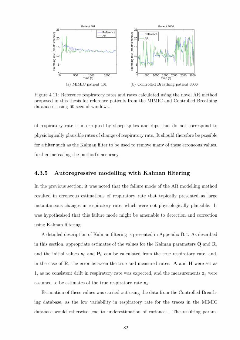
0 500 1000 15000

5

10

15

20

25

Time (s)

Bre

athi

ng r

ate

(bre

aths

/min

ute)

Patient 401

ReferenceAR

(a) MIMIC patient 401

0 500 1000 1500 2000 2500 30000

5

10

15

20

25

Time (s)

Bre

athi

ng r

ate

(bre

aths

/min

ute)

Patient 3006

Reference

AR

(b) Controlled Breathing patient 3006

Figure 4.11: Reference respiratory rates and rates calculated using the novel AR methodproposed in this thesis for reference patients from the MIMIC and Controlled Breathingdatabases, using 60-second windows.

of respiratory rate is interrupted by sharp spikes and dips that do not correspond to

physiologically plausible rates of change of respiratory rate. It should therefore be possible

for a filter such as the Kalman filter to be used to remove many of these erroneous values,

further increasing the method’s accuracy.

4.3.5 Autoregressive modelling with Kalman filtering

In the previous section, it was noted that the failure mode of the AR modelling method

resulted in erroneous estimations of respiratory rate that typically presented as large

instantaneous changes in respiratory rate, which were not physiologically plausible. It

was hypothesised that this failure mode might be amenable to detection and correction

using Kalman filtering.

A detailed description of Kalman filtering is presented in Appendix B.4. As described

in this section, appropriate estimates of the values for the Kalman parameters Q and R,

and the initial values x0 and P0 can be calculated from the true respiratory rate, and,

in the case of R, the error between the true and measured rates. A and H were set as

1, as no consistent drift in respiratory rate was expected, and the measurements zk were

assumed to be estimates of the true respiratory rate xk.

Estimation of these values was carried out using the data from the Controlled Breath-

ing database, as the low variability in respiratory rate for the traces in the MIMIC

database would otherwise lead to underestimation of variances. The resulting param-

82

x0 P0 Q R A H30 s windows 11 25 3 35 1 160 s windows 11 20 1 25 1 1

Table 4.7: Estimated Kalman filter parameters for estimated respiratory rates using ARmodelling

eters in Table 4.7 were estimated for both 30 and 60-second windows, using the results

from the AR modelling tests carried out in the previous section.

30 s window 60 s windowMIMIC CB MIMIC CB

Mean error 0.47 3.53 0.35 2.695-95% errors 0.01–2.43 0.14–11.2 0.01–1.80 0.09–8.49Improvement 0.10 0.85 0.04 0.64

Table 4.8: Results from Kalman filtering of AR-derived estimates of respiratory rate.Mean and 5–95% percentile errors are calculated from absolute errors in respiratory ratein breaths/minute. Improvements in mean error from raw estimates are also shown.

Kalman filtering using the estimated parameters in Table 4.7 was carried out on

the AR-derived estimates of respiratory rate from the MIMIC and Controlled Breath-

ing databases. The value of the Kalman estimator, x, at each iteration was used as the

estimated respiratory rate for that window.

0 500 1000 15000

5

10

15

20

Time (s)

Bre

athi

ng r

ate

(bre

aths

/min

ute)

Patient 401

ReferenceKalman

(a) MIMIC patient 401

0 500 1000 1500 2000 2500 30000

5

10

15

20

25

Time (s)

Bre

athi

ng r

ate

(bre

aths

/min

ute)

Patient 3006

Reference

Kalman

(b) Controlled Breathing patient 3006

Figure 4.12: Reference respiratory rates and Kalman filtered rates from AR modelling forselected patients from the MIMIC and Controlled Breathing databases, using 60-secondwindows.

Table 4.8 shows that Kalman filtering improved the mean error in both the MIMIC

and Controlled Breathing databases, resulting in the lowest error rates of any method

investigated in this section. Figure 4.12 shows the resulting estimated respiratory rate for

83

the same two patients as Figure 4.11. Comparison of these figures shows that Kalman fil-

tering reduced the impact of erroneous short-term deviations in the estimated respiratory

rate, while retaining the ability to follow true changes in rate.

4.3.6 Summary of results for methods using amplitude modu-

lation

Table 4.8 summarises the mean absolute errors for the best-performing method from

each of the four classes of methods assessed for their ability to estimate respiratory rates

from amplitude modulation of the PPG waveform. The results in this table show that

autoregressive modelling produced the most accurate estimates of respiratory rate, and

was further improved by the application of Kalman filtering.

30 s window 60 s windowMIMIC CB MIMIC CB

Digital filtering 0.84 4.19 0.43 3.71Fourier transforms 0.72 6.59 0.75 7.16Continuous wavelet transforms 1.55 3.99 1.30 3.55Autoregressive modelling 0.57 4.38 0.39 3.33with Kalman filtering 0.47 3.53 0.35 2.69

Table 4.9: Summary of mean absolute errors (breaths/minute) for the methods tested inthis section.

The failure modes of the other three classes of methods typically led to the estimation

of an incorrect respiratory rate corresponding to a lower, but physiologically plausible,

rate than the correct rate. This was particularly obvious for the periods of high respiratory

rate in the Controlled Breathing database, which have also been shown to display large

variations in the instantaneous respiratory rate (Figure 4.21). Although this level of

variation was likely to be due to the way in which this data was collected, by requiring

subjects to breathe in time with a metronome at rates higher than would be expected in

tidal breathing for healthy adults, it should be noted that such irregularities may appear

in spontaneously-breathing subjects due to breathing patterns associated with speech or

breathing difficulties.

84

4.4 Measuring breathing from frequency modulation

of the PPG

Section 3.3.2 showed that pre-processing of the PPG to obtain a tachogram is neces-

sary when estimating the respiratory rate from frequency modulation of the PPG. The

regularly-sampled tachogram can then be analysed in a similar way to the raw or pre-

filtered PPG when measuring respiratory rate using amplitude modulation, as shown in

Figure 3.3. Section 4.3 investigated a number of methods for analysing this type of sig-

nal in the context of amplitude modulation of the PPG, and showed that autoregressive

modelling with Kalman filtering produced the most accurate estimates of respiratory rate.

This section reports on the accuracy of methods that were not suitable for investigation

in an AM context. The results obtained with these methods will be compared to those

obtained using autoregressive modelling, which was shown to be the best performing

method for amplitude-modulated data.

4.4.1 Tachogram generation

As demonstrated in Figure 3.3, tachogram generation involves optional pre-filtering, fol-

lowed by salient point detection. A tachogram is created from the differences in time

between consecutive salient points. This tachogram is irregularly sampled, and so typi-

cally needs to be resampled to a fixed sample rate before analysis.

Table 3.1 shows that three different salient points on the PPG are used in the literature

for tachogram generation. These are the dicrotic notch (Bolanos et al., 2006), the point

of maximum slope (Lu et al., 2008), and the systolic peak (Selvaraj et al., 2008, 2009; Li

et al., 2010).

The use of the dicrotic notch as a salient point is not suitable for the MIMIC and

Controlled Breathing databases. Dicrotic notches were absent from the PPG waveforms of

many records in the MIMIC and Controlled Breathing databases. The method described

in Lu et al. (2008) for identifying the salient point at the maximum downward slope is

complex, and is not as amenable to manual verification as methods based on the dicrotic

notch or systolic peak. The systolic peak was the most frequently used method reported in

85

the literature, and was also a logical choice for a salient point which is comparable to the R

peak of the ECG. The QRS complex of the ECG is caused by ventricular depolarisation,

corresponding to ventricular contraction in the normal heart (Jevon, 2002). As peak

systole is caused by ventricular contraction, it might be expected that the timing of the

R peak of the ECG and the systolic peak of the PPG should differ only by a constant

offset, corresponding to the time taken for the arterial pressure wave to travel from the

heart to the location of the pulse oximeter finger probe. It was therefore decided that the

systolic peak would be used as a salient point for this investigation.

Detection of the systolic peaks in the PPG waveform was carried out by first removing

the baseline wander in the signal, which could otherwise mask some peaks, and prevent

them from being detected. This was achieved using a high pass filter designed using a

Kaiser windowing function, with a transition band from 0.1–0.15 Hz (6–9 breaths/minute),

5% ripple in the pass band, and 30 dB of attenuation in the stop band. The peaks in

the filtered waveform were then detected using the extrema detection algorithm described

in Appendix B.2, with a minimum delay of 0.5 s between extrema, corresponding to a

maximum detectable heart rate of 120 beats/minute.

0 5 10 15 20 25 30−1

0

1

PP

G

0 5 10 15 20 25 30

0.75

0.8

Tac

hogr

am

0 5 10 15 20 25 30

0.75

0.8

Res

ampl

ed

Time (s)

Figure 4.13: Tachogram generation from the PPG: salient point detection, raw tachogram,and resampling with cubic splines. The y-axes of the lower two graphs are in units ofseconds.

Once salient points have been detected from the PPG waveform, they can be used to

86

derive a tachogram, or time series of intervals between salient points, as shown in Figure

4.13. This is an unevenly sampled time series, with samples co-located with the second

salient point in the interval. As the salient point detection is not perfect, particularly

in regions of noisy PPG, peaks may be ‘missed’, resulting in artefactually long intervals.

These intervals appear on the tachogram as large spikes, and must be removed to ensure

that they do not mask breathing-synchronous variation in the signal.

To identify spikes on the tachogram corresponding to missed beats, it was assumed

that the heart rate, and hence the time interval between salient points, was approximately

constant over windows of 30 consecutive heart beats (at a normal adult heart rate of 60

beats/minute, this corresponds to approximately 30 seconds). Sliding windows of 30

salient points were therefore processed, with an overlap of 10 points between consecutive

windows. For each window, the median interval was calculated, and any interval that was

longer than 180% of the median was discarded, as it was likely to contain missing beats.

The choice of 180% as the threshold for detecting missed beats was determined empirically

by testing the algorithm with varying thresholds to assess the ability to identify missed

peaks reliably, while retaining robustness to variations in heart rate during the 30-point

window.

All of the analysis methods in Figure 3.3 require input signals which are regularly

sampled in time. This is not the case with the raw tachogram, which is unevenly sampled

in time. Cubic splines were therefore used to interpolate the tachogram at a specified

sampling frequency. Cubic spline interpolation has been shown to increase low-frequency

components of heart rate variation, and decrease high-frequency components (including

those due to respiratory sinus arrhythmia); the effect of this is less than with linear

interpolation, and is likely to be less pronounced at the higher heart rates observed in

children (Clifford and Tarassenko, 2005). However, the presence of artefactual intervals

due to missed beats, additional (ectopic) beats, or noise will tend to decrease the spectral

accuracy of the cubic spline interpolation. When carrying out cubic spline interpolation,

care must be taken to avoid any extrapolation, as the nature of the tachogram means

that points extrapolated using cubic splines are likely to be inaccurate.

The choice of frequency at which the tachogram was resampled using cubic splines was

87

determined by the method to be applied to the data. For example, low pass filtering with

a cut-off of 5 Hz, as specified by Correa et al. (2008), is not valid unless the signal has

been resampled at a frequency higher than 10 Hz, so that the Nyquist frequency is above

the cut-off frequency for the filter. For autoregressive modelling by the method described

in the previous section, however, resampling at a rate higher than 2 Hz is of little benefit,

as the signal will be decimated to this frequency to ensure accuracy in determining the

pole angles. It was therefore decided that the reported resampling rate from the literature

would be used for each method.

4.4.2 Digital filtering

None of the digital filtering methods investigated in Section 4.3 showed better performance

than autoregressive modelling when estimating respiratory rate from AM modulation of

the PPG, and so they were not assessed in the context of FM modulation. However,

the method proposed by Correa et al. (2008) needed to be re-considered; this was not

appropriate for testing in the AM domain, as it employed a low-pass filter with a cut-off

frequency of 5 Hz. In the AM domain, frequencies corresponding to the heart rate would

be within the pass-band, and so the method would be unlikely to give accurate estimates

of the respiratory rate. In the analysis of a tachogram, however, it was not expected that

heart rate frequencies would have a large influence, and so this method could be effective

in this context.

0 10 20 30 40 50 600.75

0.8

0.85

Tac

hogr

am

0 10 20 30 40 50 60

0.8

0.9

Filt

ered

0 10 20 30 40 50 60−2

0

2

Ref

eren

ce

Time (s)

Figure 4.14: Comparison of PPG tachogram-derived waveform from digital filtering usingthe method proposed by Correa et al. (2008) and the reference respiratory waveform, withdetected breaths shown in black.

The raw tachogram was interpolated to 100 Hz using cubic splines, as described in

88

Correa et al. (2008). As described in the paper, the signal was then filtered using an FIR

filter with an order of 1500, and a cut-off frequency of 5 Hz. Since Correa et al. (2008)

did not apply a method for calculating the respiratory rate from the filtered signal, the

simple breath detection algorithm described in Appendix B.2 was used. The operation of

this method on sample data from the MIMIC database is shown in Figure 4.14.

60 s window 120 s windowMIMIC CB MIMIC CB

Mean error 3.19 3.48 3.31 3.455-95% errors 0.22–8.61 0.16–10.5 0.22–8.76 0.14–10.5

Table 4.10: Results from tests using the digital filtering method proposed by Correa et al.(2008) on tachogram data derived from the PPG. Mean and 5–95% percentile errors arecalculated from absolute errors in respiratory rate in breaths/minute.

Table 4.10 shows the results from applying the method proposed by Correa et al.

(2008) to the data in the MIMIC and Controlled Breathing databases. This shows that

the performance of the method did not differ greatly when applied to different window

lengths or databases. The graphs in Figure 4.15 show the performance of the method

on two of the records from the MIMIC and Controlled Breathing databases, and shows

that there was considerable variation in the estimated respiratory rates, with the method

struggling to cope with the high rates seen in the Controlled Breathing database. As with

the digital filtering methods investigated in Section 4.3, the failure mode of this method

resulted in a respiratory rate that was consistent with normal breathing, so that it would

be difficult to detect or correct such failures.

4.4.3 Autocorrelation function

Schafer and Kratky (2008) described two different methods for deriving respiratory rate

using the autocorrelation function. However, as discussed in Section 3.3.2, the description

of the more complex method, termed ’acf-adv’, was unclear, and so was not implemented.

The simpler method, termed ‘acf-max’ in the paper, calculated the autocorrelation

function of a tachogram which has been interpolated at a sampling frequency of 5 Hz

using cubic splines. The resulting autocorrelation function was then interpolated using

cubic splines to enable more accurate location of the first peak, as shown in Figure 4.16.

89

0 500 1000 15000

5

10

15

20

25

Time (s)

Bre

athi

ng r

ate

(bre

aths

/min

ute)

Patient 401

ReferenceFiltering

(a) MIMIC patient 401

0 500 1000 1500 2000 2500 30000

5

10

15

20

25

Time (s)

Bre

athi

ng r

ate

(bre

aths

/min

ute)

Patient 3006

Reference

Filtering

(b) Controlled Breathing patient 3006

Figure 4.15: Reference respiratory rates and rates calculated using the method proposedby Correa et al. (2008) for selected patients from the MIMIC and Controlled Breathingdatabases, using 60-second windows.

The lag δmax at this peak was used to calculate the respiratory rate as 60/(δmaxfs), where

fs = 5 is the sampling rate of the tachogram after cubic spline interpolation. As discussed

in Section 4.3, this method was not appropriate for application in the AM domain, and

so it was decided to test it using the PPG-derived tachogram.

0 10 20 30 40 50 600.75

0.8

0.85

Tac

hogr

am

Time (s)

0 20 40 60 80 100−1

0

1

AC

F

0 20 40 60 80 100−1

0

1

Inte

rpol

atio

n

Lag

Figure 4.16: Estimation of respiratory rate from the PPG-derived tachogram using the‘acf-max’ autocorrelation method proposed by Schafer and Kratky (2008). The detectedpeak corresponding to the estimated respiratory rate is shown by a red cross.

The method was implemented using a 10-fold interpolation of the lags (i.e. the inter-

polated autocorrelation function had 10 times as many points as the original signal). To

remove the influence of very early peaks due to the cubic spline fitting, any peak corre-

sponding to a lag of less than 3 was eliminated. The maximum lag was set to be 100,

corresponding to a respiratory rate of 3 breaths/minute.

90

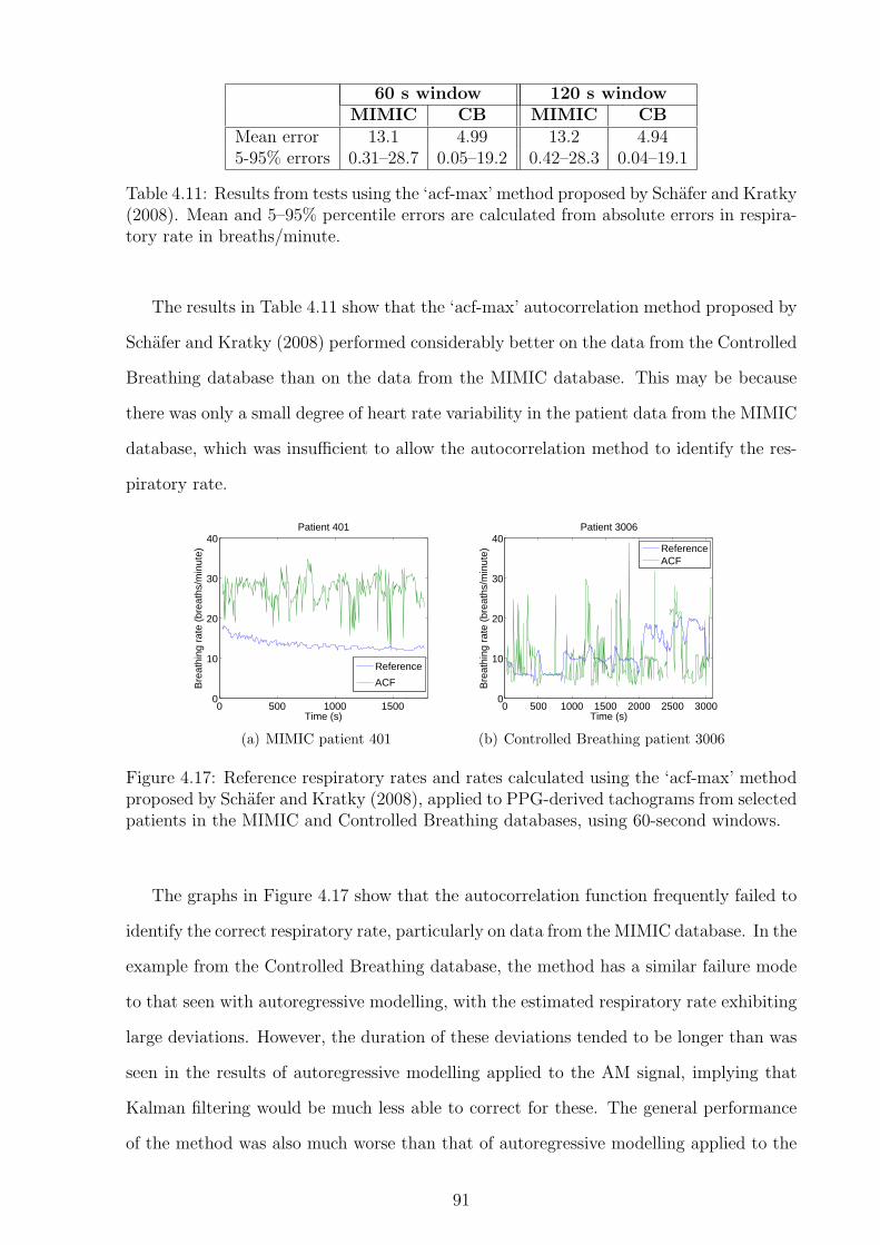
60 s window 120 s windowMIMIC CB MIMIC CB

Mean error 13.1 4.99 13.2 4.945-95% errors 0.31–28.7 0.05–19.2 0.42–28.3 0.04–19.1

Table 4.11: Results from tests using the ‘acf-max’ method proposed by Schafer and Kratky(2008). Mean and 5–95% percentile errors are calculated from absolute errors in respira-tory rate in breaths/minute.

The results in Table 4.11 show that the ‘acf-max’ autocorrelation method proposed by

Schafer and Kratky (2008) performed considerably better on the data from the Controlled

Breathing database than on the data from the MIMIC database. This may be because

there was only a small degree of heart rate variability in the patient data from the MIMIC

database, which was insufficient to allow the autocorrelation method to identify the res-

piratory rate.

0 500 1000 15000

10

20

30

40

Time (s)

Bre

athi

ng r

ate

(bre

aths

/min

ute)

Patient 401

Reference

ACF

(a) MIMIC patient 401

0 500 1000 1500 2000 2500 30000

10

20

30

40

Time (s)

Bre

athi

ng r

ate

(bre

aths

/min

ute)

Patient 3006

ReferenceACF

(b) Controlled Breathing patient 3006

Figure 4.17: Reference respiratory rates and rates calculated using the ‘acf-max’ methodproposed by Schafer and Kratky (2008), applied to PPG-derived tachograms from selectedpatients in the MIMIC and Controlled Breathing databases, using 60-second windows.

The graphs in Figure 4.17 show that the autocorrelation function frequently failed to

identify the correct respiratory rate, particularly on data from the MIMIC database. In the

example from the Controlled Breathing database, the method has a similar failure mode

to that seen with autoregressive modelling, with the estimated respiratory rate exhibiting

large deviations. However, the duration of these deviations tended to be longer than was

seen in the results of autoregressive modelling applied to the AM signal, implying that

Kalman filtering would be much less able to correct for these. The general performance

of the method was also much worse than that of autoregressive modelling applied to the

91

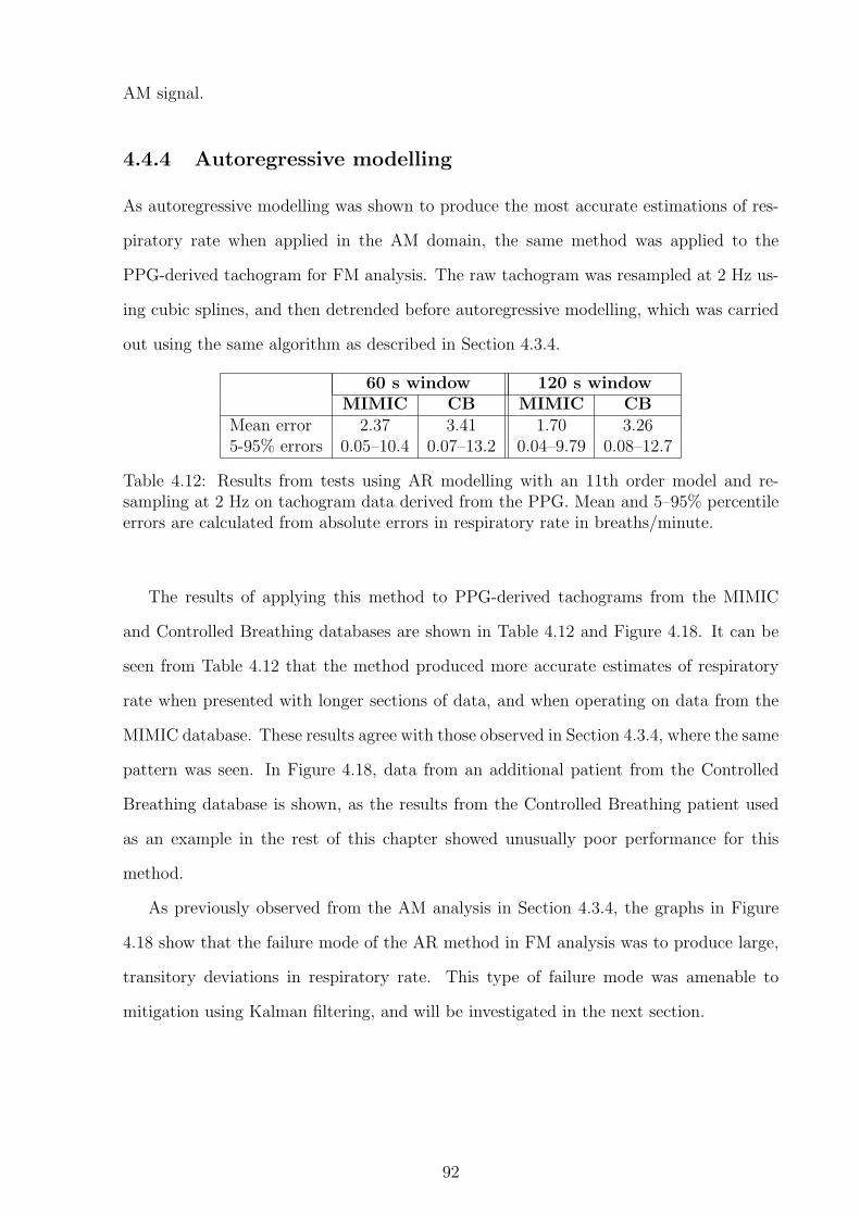
AM signal.

4.4.4 Autoregressive modelling

As autoregressive modelling was shown to produce the most accurate estimations of res-

piratory rate when applied in the AM domain, the same method was applied to the

PPG-derived tachogram for FM analysis. The raw tachogram was resampled at 2 Hz us-

ing cubic splines, and then detrended before autoregressive modelling, which was carried

out using the same algorithm as described in Section 4.3.4.

60 s window 120 s windowMIMIC CB MIMIC CB

Mean error 2.37 3.41 1.70 3.265-95% errors 0.05–10.4 0.07–13.2 0.04–9.79 0.08–12.7

Table 4.12: Results from tests using AR modelling with an 11th order model and re-sampling at 2 Hz on tachogram data derived from the PPG. Mean and 5–95% percentileerrors are calculated from absolute errors in respiratory rate in breaths/minute.

The results of applying this method to PPG-derived tachograms from the MIMIC

and Controlled Breathing databases are shown in Table 4.12 and Figure 4.18. It can be

seen from Table 4.12 that the method produced more accurate estimates of respiratory

rate when presented with longer sections of data, and when operating on data from the

MIMIC database. These results agree with those observed in Section 4.3.4, where the same

pattern was seen. In Figure 4.18, data from an additional patient from the Controlled

Breathing database is shown, as the results from the Controlled Breathing patient used

as an example in the rest of this chapter showed unusually poor performance for this

method.

As previously observed from the AM analysis in Section 4.3.4, the graphs in Figure

4.18 show that the failure mode of the AR method in FM analysis was to produce large,

transitory deviations in respiratory rate. This type of failure mode was amenable to

mitigation using Kalman filtering, and will be investigated in the next section.

92

0 500 1000 15000

5

10

15

20

25

Time (s)

Bre

athi

ng r

ate

(bre

aths

/min

ute)

Patient 401

Reference

AR

(a) MIMIC patient 401

0 500 1000 1500 2000 2500 30000

5

10

15

20

25

Time (s)

Bre

athi

ng r

ate

(bre

aths

/min

ute)

Patient 3006

Reference

AR

(b) Controlled Breathing patient 3006

0 1000 2000 30000

5

10

15

20

25

30

Time (s)

Bre

athi

ng r

ate

(bre

aths

/min

ute)

Patient 3002

Reference

AR

(c) Controlled Breathing patient 3002

Figure 4.18: Reference respiratory rates and rates calculated using the novel AR methodproposed in this thesis, applied to PPG-derived tachograms from selected patients in theMIMIC and Controlled Breathing databases, using 60-second windows.

4.4.5 Autoregressive modelling with Kalman filtering

The results of the tests carried out on the PPG-derived tachograms showed that autore-

gressive modelling produced the most accurate estimates of respiratory rate. As was seen

in Section 4.3.4, the failure mode of the AR modelling method when applied to the PPG-

derived tachogram resulted in large instantaneous changes in respiratory rate, which were

typically of short duration. Section 4.3.5 showed that this type of failure mode could be

mitigated by the application of a Kalman filter, and so Kalman filtering was also applied

to the autoregressive modelling results from this section.

x0 P0 Q R A H60 s windows 11 20 1 25 1 1120 s windows 11 20 0.2 25 1 1

Table 4.13: Estimated Kalman filter parameters for respiratory rates calculated using ARmodelling on PPG-derived tachograms

The Kalman filter parameters were derived from the Controlled Breathing database

93

results for both 60 and 120-second windows using the same approach as was described in

Section 4.3.5. The resulting estimated parameters are shown in Table 4.13. Comparison

of these values with those in Table 4.7 shows that the values for the 60-second windows

match, with the exception of R, which is the only parameter that depends on the error

between the true and estimated rates.

60 s window 120 s windowMIMIC CB MIMIC CB

Mean error 1.77 2.64 1.48 2.385-95% errors 0.04–6.83 0.08–10.2 0.03–6.24 0.09–8.91Improvement 0.61 0.77 0.22 0.88

Table 4.14: Results from Kalman filtering of AR-derived estimates of respiratory ratefrom PPG-derived tachogram data. Mean and 5–95% percentile errors are calculatedfrom absolute errors in respiratory rate in breaths/minute. Improvements in mean errorfrom raw estimates are also shown.

Kalman filtering was carried out on the estimates of respiratory rate obtained from AR

modelling of the PPG-derived tachogram. As in Section 4.3.5, the value of the Kalman

estimator, x, at each iteration was assigned to be the estimated respiratory rate for

that window. Table 4.13 shows the errors in respiratory rate after Kalman filtering,

demonstrating that there was an improvement in the error as a result of the Kalman

filtering.

Figure 4.19 shows the estimated respiratory rates after Kalman filtering for the three

patients shown in Figure 4.17. Comparison of these figures shows that the effect of short

term deviations from the true respiratory rate was decreased by Kalman filtering, without

a significant impact on the ability of the method to follow true changes in respiratory rate.

4.4.6 Summary of results from methods using frequency mod-

ulation

Table 4.15 summarises the mean absolute errors of respiratory rate for the methods applied

to the PPG tachogram in this section. As in the case of AM modulation, it can be seen

that autoregressive modelling provided the most accurate estimates of respiratory rate,

and that these estimates were further improved by Kalman filtering.

The results of autoregressive modelling with Kalman filtering can be compared for both

94

0 500 1000 15000

5

10

15

20

25

Time (s)

Bre

athi

ng r

ate

(bre

aths

/min

ute)

Patient 401

ReferenceKalman

(a) MIMIC patient 401

0 500 1000 1500 2000 2500 30000

5

10

15

20

25

Time (s)

Bre

athi

ng r

ate

(bre

aths

/min

ute)

Patient 3006

Reference

Kalman

(b) Controlled Breathing patient 3006

0 1000 2000 30000

5

10

15

20

25

30

Time (s)

Bre

athi

ng r

ate

(bre

aths

/min

ute)

Patient 3002

Reference

Kalman

(c) Controlled Breathing patient 3002

Figure 4.19: Reference respiratory rates and rates calculated using the novel AR methodproposed in this thesis on PPG-derived tachogram data from selected patients in theMIMIC and Controlled Breathing databases, using 60-second windows.

AM and FM analysis of the PPG using 60-second windows. For the MIMIC database, the

mean errors were 0.35 breath/minute for AM analysis, and 1.77 breaths/minute for FM

analysis. When assessing data from the Controlled Breathing database, the equivalent

errors were 2.69 breaths/minute for AM analysis, and 2.64 breaths/minute for FM anal-

ysis. As shown in Figure 4.22, the level of heart rate variation was very low in the data

from the MIMIC database, which may explain why AM analysis of this data provided

better results than FM analysis. There was little difference in the accuracy of AM- and

60 s window 120 s windowMIMIC CB MIMIC CB

Digital filtering 3.19 3.48 3.31 3.45Autocorrelation function 13.1 4.99 13.2 4.94Autoregressive modelling 2.37 3.41 1.70 3.26with Kalman filtering 1.77 2.64 1.48 2.38

Table 4.15: Summary of mean absolute errors (breaths/minute) for the methods testedin this section.

95

FM-derived respiratory rate estimates for data from the Controlled Breathing database

using autoregressive modelling.

4.5 Summary

The Controlled Breathing database produced less accurate estimates of respiratory rate

than the MIMIC database for the majority of methods. This may have been partly

due to the more challenging nature of the data (such as the wider range of respiratory

rates, presence of apnoeas, and variation in rate), but was also likely to be influenced

by the remaining presence of large baseline variations on the PPG signals, even after

pre-processing, and the fact that the subjects were breathing at particular rates under

conscious control, which may lead to less regular breathing. Although the resolution of

the PPG in the Controlled Breathing database was higher than that of the MIMIC PPG

signal (15-bit compared to 12-bit), the potential for greater accuracy in the original signal

appears to have been outweighed by the problems introduced by issues such as baseline

variation.

0 500 1000 1500−1

−0.5

0

0.5

1Patient 401

Time (s)

PP

G

(a) MIMIC patient 401

0 1000 2000 3000−3000

−2000

−1000

0

1000

2000

3000Patient 3010

Time (s)

PP

G

(b) Controlled Breathing patient 3010

Figure 4.20: Comparison of baseline variation after preprocessing in PPGs from theMIMIC and Controlled Breathing databases. The y-axes of these graphs are shown in theraw units provided by the data sources, and so are not directly comparable.

Figure 4.20 shows that the baseline variation on the Controlled Breathing data, even

after pre-processing, was vastly greater than that on the data from the MIMIC database.

The difference in baseline variation between the two sets of data is likely to be due to

differences in the hardware used to obtain the signals, with the hardware used to collect

96

the MIMIC data potentially using some form of compensation to ensure a minimum

amount of baseline wander. On this basis, no further attempts were made to reduce

baseline wander in the data from the Controlled Breathing database, as this problem has

clearly already been solved by some pulse oximeter manufacturers. It is possible that

the MIMIC data also had automatic gain control applied to the signal before recording.

However, as this would be expected to affect the AM analysis, which generally performed

better on this database, the effect is likely to have been minor.

0 500 1000 150010

15

20

25

30Patient 444

Time (s)

Res

pira

tory

rat

e (b

reat

hs/m

inut

e)

(a) MIMIC patient 444

2000 2500 3000 350010

15

20

25

30Patient 3007

Time (s)

Res

pira

tory

rat

e (b

reat

hs/m

inut

e)

(b) Controlled Breathing patient 3007

Figure 4.21: Comparison of variation of instantaneous respiratory rate for MIMIC andControlled Breathing patients breathing at approximately 20 breaths/minute.

The worst results for the Controlled Breathing data occured, for all methods, when

the subjects were breathing at the faster respiratory rate, which was approximately 20

breaths/minute. Since the subjects included in this database were required to match

their breathing rate to a metronome, a possible cause of this is that this forced (i.e.

non-spontaneous) breathing resulted in an irregular instantaneous respiratory rate. This

would be expected to be most noticeable at high respiratory rates, as a small error in

breath timing by the subject would result in a large change in instantaneous rate. In

addition, the higher rate of 20 breaths/minute is outside the normal range of respiratory

rates for a resting adult, and so the subjects may not have been achieving adequate gas

exchange. This would lead to signals from the autonomic nervous system to slow down

the respiratory rate, and so the subjects may have found it more difficult to consciously

maintain this rate. Figure 4.21 compares typical subjects from both databases breathing

at a similar rate of around 20 breaths/minute, and clearly shows that the instantaneous

respiratory rate shows much greater variation in the Controlled Breathing database. It

97

should be noted that the patients in the MIMIC database were seriously ill, and so the

regular respiratory rate for the MIMIC patient shown in Figure 4.21 was likely to be due

to artificial ventilation. Spontaneously breathing patients are therefore likely to have more

variable respiratory rates than those seen in the MIMIC database. Since the patients in the

Controlled Breathing database were not breathing spontaneously, it was not clear whether

spontaneous breathing would result in more or less consistent instantaneous respiratory

rates than those seen in the Controlled Breathing database. However, other factors such

as speech may cause greater irregularities in respiratory rates than are seen in either

database considered here, and are therefore likely to lead to more challenging signals in

conscious patients.

Respiratory rates calculated using longer windows were generally more accurate. How-

ever, the length of the window determined the minimum amount of data required to cal-

culate an initial respiratory rate, which is an important consideration in the context of

paediatric triage. A 60-second window appeared to be an acceptable compromise between

accuracy and practicality.

Autoregressive modelling produced the most accurate estimates of respiratory rate

from the PPG. In addition, Kalman filtering was shown to increase the accuracy of both

AM- and FM-derived respiratory rates calculated using autoregressive modelling.

0 500 1000 15000

20

40

60

80

100Patient 253

Time (s)

Hea

rt r

ate

(bea

ts/m

inut

e)

(a) MIMIC patient 253

0 1000 2000 30000

20

40

60

80

100Patient 3002

Time (s)

Hea

rt r

ate

(bea

ts/m

inut

e)

(b) Controlled Breathing patient 3002

Figure 4.22: Comparison of variation of instantaneous heart rate (derived from the ECG)for MIMIC and Controlled Breathing patients.

FM-derived respiratory rates calculated using autoregressive modelling were less ac-

curate than AM-derived rates for patients from the MIMIC database, although a similar

pattern was not seen in the results from patients in the Controlled Breathing database.

98

This may have been due to a low level of respiratory sinus arrhythmia in the patients

in the MIMIC database, as might be expected when monitoring seriously ill patients.

Figure 4.22 demonstrates that heart rate variation is indeed lower in MIMIC patients.

The data in this figure is derived from R-peak detection in the ECG, as both the MIMIC

and Controlled Breathing databases also contained ECG information, which allowed more

accurate measurement of heart rate than might be possible with the PPG alone.

Based on the results presented in this chapter, estimation of respiratory rate from

paediatric PPG data was carried out using autoregressive modelling and Kalman filter-

ing. Both amplitude and frequency modulation were investigated on data collected from

children.

It was necessary to adjust the methods for pre-processing of the PPG waveform and

choosing an appropriate pole from the autoregressive model to allow for the larger range

of respiratory rates observed in children. As shown in Chapter 2, the range of potential

respiratory rates during childhood is much greater than that expected in adolescence or

adulthood.

99

Chapter 5

Respiratory rate estimation in

children

In Chapter 4, autoregressive modelling with Kalman filtering was shown to produce the

most accurate estimates of respiratory rate from PPG waveforms collected from adult

subjects. Since no data sources containing PPG waveforms obtained from children were

available at the start of the project, two studies were set up to collect paediatric pulse

oximetry data and associated respiratory rate information. The following section describes

these two studies; the Oxford School study and the OXEMS study.

This chapter then discusses adjustments to the methods applied in Chapter 4 to make

them applicable to paediatric data, and reports the results of applying the adjusted meth-

ods to the data collected in the Oxford School Study and OXEMS study.

5.1 Collection of paediatric pulse oximetry and res-

piratory rate data

5.1.1 The Oxford School study

The Oxford School study was carried out on 29 June 2007 at a primary school in Oxford.

Ethics approval for the study was obtained from the Oxford Research Ethics Committee.

Consent to having their vital signs measured was obtained for thirty-six children from

Years 5 and 6 (16 female, 20 male). The children were aged between 8 and 11 years, with

100

a mean age of 9.9 years on the day of the study. Two separate Visi-3 systems (Stowood

Scientific Instruments, Beckley, Oxon) were used to measure the children’s vital signs

before, during, and after two to three minutes of vigorous exercise (cycling on an exercise

bicycle), with a typical recording length of 7 minutes.

The Visi-3 system allows a wide range of physiological variables to be measured using

a variety of sensors, only a few of which were used in this study. Table 5.1 shows the

measurements made during this study, with Figure 5.1 showing the placement of the

sensors.

Figure 5.1: Laboratory co-worker demonstrating placement of sensors for the OxfordSchool study

Parameter Sample rate SensorThoracic effort 256 Hz thoracic bandAbdominal effort 256 Hz abdominal bandNasal airflow 128 Hz nasal cannulaNasal sound 128 Hz nasal cannulaPPG waveform 256 Hz pulse oximeterSpO2 1 Hz pulse oximeterPulse rate 1 Hz pulse oximeterPulsatile index 1 Hz pulse oximeter

Table 5.1: Measurements made using the Visi-3 system during the Oxford School study

The nasal cannula used in the study is a narrow gauge plastic tube with two prongs

that fit into the nares, allowing airflow and sound measurements to be made. As some

101

people find this uncomfortable, the children in the study were given the choice of not

having a cannula fitted, in which case only the abdominal and thoracic effort bands

would be used for breathing measurement. However, over 90% of the children consented

to having the cannula fitted, with over 85% retaining the cannula in place for the whole

recording.

All of the children had two respiratory effort bands fitted. These are made of an elastic

material with an integral wire, so that changes in the circumference of the band result

in a change in the the inductance of the wire. The bands were placed around the chest

(outside the child’s clothing) at nipple level, and around the abdomen at the level of the

navel. Two different sizes of bands were available (medium and large), and were chosen

based on the size of the child.

A standard pulse oximeter was used to measure the PPG, pulse rate, SpO2, and

pulsatile index. The finger probe was placed on the child’s middle or index finger. Both

paediatric and adult probes were available, with most children (92%) being fitted with a

paediatric probe. The adult probe was used where the signal quality using the paediatric

probe was observed to be poor, or where the clinical judgement of the researchers indicated

that this was likely to be the case.

The data recorded by the Visi-3 system can be extracted as a text file, and this facility

was used to import the data into Matlab for further processing. Appendix A.1.3 describes

the pre-processing applied to the Visi-3 waveforms before analysis.

5.1.2 The OXEMS study

The OXEMS study was carried out at the OXEMS out-of-hours GP centre in Oxford

between March and June 2009. As well as providing pulse oximetry and respiratory rate

data from unwell children over a wide age range, the study allowed the feasibility of the

proposed paediatric triage system to be assessed in a clinical environment.

Hardware and software

Figure 5.2 shows the hardware used in the OXEMS study. The Nonin 4100 pulse oximeter

(Nonin Medical, Plymouth, MN, USA) monitored SpO2, heart rate, peripheral perfusion,

102

(a) Nonin 4100 Bluetooth PulseOximeter

(b) Spot LXi Vital Signs moni-tor

(c) Visensia tablet PC

Figure 5.2: Hardware used in the OXEMS study

and the PPG waveform, and transmitted the data using a wireless Bluetooth radio link.

The Spot LXi Vital Signs monitor (Welch Allyn, Skaneateles Falls, NY, USA) was used

to measure axillary temperature using a SureTemp Plus thermocouple probe, which can

measure axillary temperature in 10–15 seconds. The temperature data was transmitted

using a serial cable.

A Visensia tablet PC (OBS Medical Ltd, Abingdon, Oxon) was used to receive data

from the pulse oximeter and thermometer. The PC displayed the vital signs measured

(SpO2, heart rate, perfusion and temperature), and allowed manual input of the measured

respiratory rate, temperature (to allow an alternative thermometer to be used) and the

patient’s date of birth. The software automatically assigned a sequential study identifi-

cation number for each child. This was also recorded on the patient consent form, and

ensured that anonymity was maintained, while still allowing verification that consent had

been obtained.

The software on the tablet PC was developed as part of the work carried out for this

thesis, using an existing code base provided by OBS Medical Ltd. This consisted of a

“client” written in C#, which communicated with the pulse oximeter and thermometer,

and transmitted the vital signs information to the “server”. The server, which was written

in a combination of C# and C++, provided the user interface for the monitor, via the

touch screen of the Visensia tablet PC.

The main screen of the user interface is shown in Figure 5.3. Recording was triggered

by the clinician requesting a new patient session, or by the arrival of new data from the

103

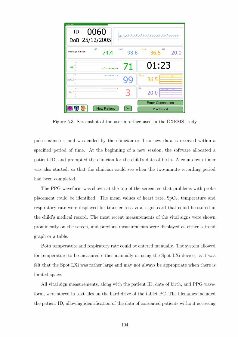
Figure 5.3: Screenshot of the user interface used in the OXEMS study

pulse oximeter, and was ended by the clinician or if no new data is received within a

specified period of time. At the beginning of a new session, the software allocated a

patient ID, and prompted the clinician for the child’s date of birth. A countdown timer

was also started, so that the clinician could see when the two-minute recording period

had been completed.

The PPG waveform was shown at the top of the screen, so that problems with probe

placement could be identified. The mean values of heart rate, SpO2, temperature and

respiratory rate were displayed for transfer to a vital signs card that could be stored in

the child’s medical record. The most recent measurements of the vital signs were shown

prominently on the screen, and previous measurements were displayed as either a trend

graph or a table.

Both temperature and respiratory rate could be entered manually. The system allowed

for temperature to be measured either manually or using the Spot LXi device, as it was

felt that the Spot LXi was rather large and may not always be appropriate when there is

limited space.

All vital sign measurements, along with the patient ID, date of birth, and PPG wave-

form, were stored in text files on the hard drive of the tablet PC. The filenames included

the patient ID, allowing identification of the data of consented patients without accessing

104

any data from patients who did not consent.

Although the Nonin 4100 pulse oximeter provides a perfusion index, it was discovered

that this was highly quantised, with only 4 possible levels. Despite collecting data on a

variety of children, a perfusion index of less than 3 (the maximum value possible) was

never observed, and so no further analysis was carried out with this parameter.

Protocol

The protocol for the OXEMS study was approved by the Mid & South Bucks Research

Ethics Committee. A total of 52 children were successfully recruited into the study, but

a reference respiratory rate was not recorded for 8 of these, resulting in a useful study

sample of 44 children. The children’s ages ranged from 1 month to 10.9 years, with a

median age of 2.8 years. Over one third of the children with vital sign measurements

(36%) were under the age of two years. Three children recruited at the start of the study

did not have their full year of birth recorded due to a software error, and so their age

could not be calculated.

All children aged between one month and ten years attending the centre with a medical

illness were eligible for inclusion in the study. Children were excluded from the study if

their condition was sufficiently serious that they went straight in to the consultation room

on arrival, or if the research nurse judged that involvement in the study would cause an

unnecessary delay before they received appropriate clinical care.

Upon arrival, children meeting the eligibility criteria were directed to the research

nurse, who was situated close to the waiting room. The nurse then performed the vital

sign measurements by attaching the pulse oximeter for at least two minutes, and taking

the child’s temperature. The nurse counted and recorded the respiratory rate twice during

the two-minute monitoring period, and also noted the child’s level of distress.

Consent for research use of the measured vital signs was obtained either before the

monitoring period, or after the child had seen a clinician, if the parents wished to have

further time to consider their decision. The ID number assigned by the software was

recorded on the consent form, so that only data collected from those who had consented

would be used for further analysis.

105

5.2 Adjustments to respiratory rate estimation algo-

rithms for use on paediatric data

Respiratory rate estimation algorithms designed for adult subjects need to be modified

before they can be used successfully to estimate respiratory rates in children. The main

reason for this is the wider range of respiratory rates observed in children, with normal

values for young children and infants far exceeding those that would be considered highly

abnormal in an adolescent or adult, as demonstrated by the meta-analysis in Chapter 2.

In addition, the lower bounds of normal heart rate in older children can overlap with the

upper bounds of normal respiratory rate in younger children. Care therefore needs to be

taken when choosing the frequency range in which to search for the pole corresponding

to the respiratory rate (the ‘breathing pole’). This needs to be wide enough to include

fast respiratory rates in young children, but narrow enough to minimise spectral leakage

from slower heart rates in older children, which could mask the breathing poles due to

their high spectral power.

The quality of signals obtained from children also leads to more challenging signal pro-

cessing than is typically the case with adult data. Children may not tolerate monitoring

equipment particularly well, and may be restless or unco-operative during the measure-

ment period. This is likely to lead to high levels of movement artefact on the recorded

waveform, with an associated reduction in signal quality. This is a particular problem

in primary or emergency care, where children, although unwell, are still generally active,

and may be fretful.

The two modifications required for the AR methods described in Chapter 4 are the

pre-processing of the PPG waveform, and the choice of the breathing pole.

5.2.1 Modification of pre-processing methods for PPG wave-

forms

Pre-processing of the PPG waveform was performed differently depending on whether

amplitude or frequency modulation was being investigated. Both types of pre-processing

required modifications for use in children.

106

The main modification required in the case of amplitude modulation of the PPG wave-

form was an adjustment to the pre-filter applied to the waveform. As higher respiratory

rates were expected in children, the cut-off frequency for the pre-filter needed to be in-

creased to ensure that respiratory frequencies were not filtered out at the pre-processing

stage. The modified low-pass filter was designed using a Kaiser windowing function, with

a 5% ripple in the pass band and 30 dB of attenuation in the stop band. The tran-

sition band was specified as 0.6–1 Hz, which corresponds to respiratory rates of 36–60

breaths/minute.

In the OXEMS study, the PPG waveform was extracted as an unsigned integer cor-

responding to the raw 16-bit signal from the pulse oximeter. The waveform had a very

large dc offset, and so an additional detrending step was introduced before the prefilter

to ensure that further signal processing would not be affected by this offset.

In the case of frequency modulation of the PPG waveform, it is necessary to identify

salient points in the signal, and use their locations in time to create a tachogram for

further analysis. As described in Section 4.4, the systolic peaks of the PPG waveform

were used to define the salient points.

Detection of the salient points in the PPG waveform was carried out as described

in Section 4.4, with the exception that the minimum delay allowed between consecutive

extrema was shortened to 0.25 seconds, which corresponds to a maximum detectable heart

rate of 240 beats/minute. This was increased from the maximum of 120 beats/minute

used in Chapter 4, to reflect the higher heart rates observed in children.

Autoregressive modelling was then carried out on 60-second windows of data, with a

5-second gap between consecutive windows. The downsampling frequency was increased

from the 2 Hz frequency used in Chapter 4, to allow for the higher expected respira-

tory rates in the paediatric data. These were expected to include rates of around 70-80

breaths/minute (1.2–1.3 Hz), which is above the Nyquist frequency of a signal downsam-

pled to 2 Hz. Downsampling frequencies were chosen to be exact divisors of the PPG

sampling frequencies in both the Oxford School Study and the OXEMS study, so that

downsampling of the PPG could be carried out without the need for interpolation. For

the Oxford School Study, a downsampling frequency of 4 Hz was chosen, and for the

107

OXEMS study, a downsampling frequency of 3 Hz was chosen. Different downsampling

frequencies were used as the two original sampling frequencies (256 Hz and 75 Hz) do not

have any common integer divisors with an appropriate Nyquist frequency. As in Chapter

4, an AR model order of 11 was used in all cases.

In addition to these pre-processing methods, a simple signal quality assessment was

carried out for each window of data to be analysed. If more than half of the window

contained invalid heart rate or SpO2 values, as reported by the pulse oximeter, then the

data in that window was considered to be of poor quality and not analysed.

5.2.2 Modification of pole-choice algorithm

The pole-choice algorithm required modification for use in children to allow the detection

of higher respiratory rates. This led to a larger sector of interest covering the angles that

correspond to potential breathing poles.

Both the AM and FM pre-processed data were analysed using the pole-choice algo-

rithm described in Chapter 4. The range of potential respiratory rates was altered to be

6–50 breaths/minute, with an extension of the range to 0–80 breaths/minute if no poles

were identified in the original range. As with the adult data, the choice of pole was made

based on the pole magnitude, with the highest magnitude pole being chosen to define the

respiratory rate.

5.3 Results of respiratory rate estimation

Respiratory rate estimation was performed on both paediatric data sets using AR mod-

elling. AR modelling was carried out using both AM and FM methods for each data set.

It was hypothesised that some of the children may exhibit reduced breathing variation in

either the AM or FM part of the signal, while retaining variation in the other part. It

was therefore thought to be helpful to use information from both AM and FM analyses

to assess the respiratory rate. Possible reasons for reduced AM variation include mask-

ing by motion artefacts, and recession (indrawing of the chest wall during inspiration)

or use of accessory muscles (e.g. shoulder muscles). These phenomena are common in

children with severe breathing difficulties, and may reduce the pressure variation in the

108

chest cavity that is thought to be a cause of AM breathing variation in the PPG. Re-

duced FM variation may be caused by medication, illness or high respiratory rates (van

Ravenswaaij-Arts et al., 1993). It is possible that some unwell or distressed children may

exhibit significant reductions in both the FM and AM variation, making it difficult to

obtain an accurate respiratory rate from their PPG.

The results presented in this section were compared against the reference respiratory

rate, and also against the ‘best possible’ pole. This pole was defined as the pole which was

closest to the reference respiratory rate in a particular window, and therefore represented

the smallest possible error in respiratory rate for that AR model. The ‘best possible’ pole

was chosen solely on the basis of the respiratory frequency, and so may have had a very

low magnitude, and hence be unlikely to be chosen by the pole selection methods. This

information is presented to allow the quality of the pole-choice algorithm to be assessed

independently from the ability of the AR model to produce accurate breathing poles.

5.3.1 Oxford School study

As described in Appendix A.1.3, a number of the records from the Oxford School study

contained periods where the reference breathing data was of very poor quality. During

these periods, the noise present on the reference respiratory waveforms masked the signal

to the extent that it was not possible to manually verify the detection of breaths, making

it difficult to ascertain the reference respiratory rate with any level of accuracy. It was

therefore decided to analyse just the 19 records with good reference data throughout the

recording. In these records, it was possible to manually verify that automated breath

detection on the reference respiratory waveforms corresponded to actual breaths, leading

to an acceptable degree of confidence in the reference respiratory rates. These 19 records

comprised just over half of the original data set of 36 recordings, and it was hypothesised

that the respiratory data in these recordings was of better quality because the children did

not talk during the recording, although it was not possible to confirm this retrospectively.

Figures 5.4–5.6 demonstrate the results obtained by analysing the data from three

children enrolled in the Oxford School study. The graphs show the raw PPG and the

pre-processed AM and FM signals, and the results from AR modelling using the AM and

109

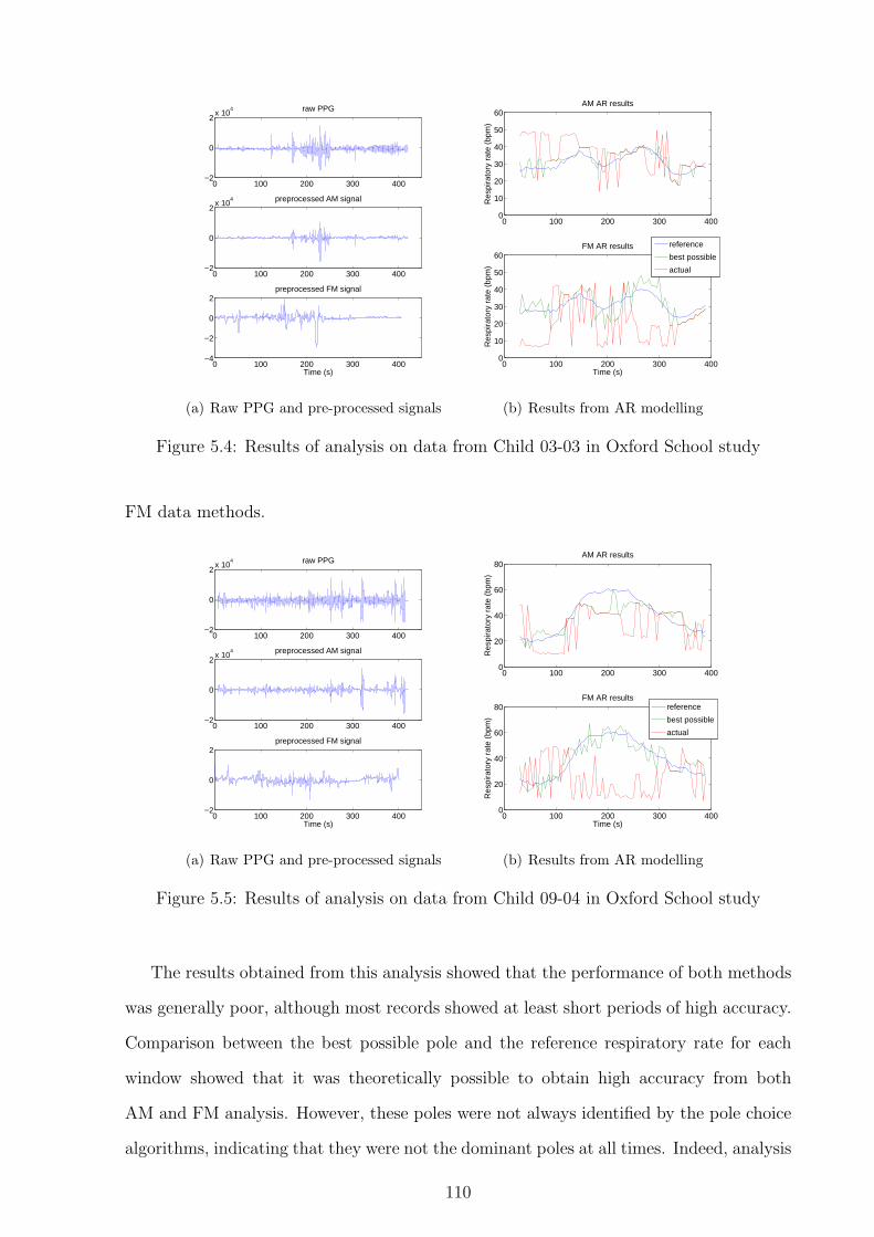
0 100 200 300 400−2

0

2x 10

4 raw PPG

0 100 200 300 400−2

0

2x 10

4 preprocessed AM signal

0 100 200 300 400−4

−2

0

2preprocessed FM signal

Time (s)

(a) Raw PPG and pre-processed signals

0 100 200 300 4000

10

20

30

40

50

60AM AR results

Res

pira

tory

rat

e (b

pm)

0 100 200 300 4000

10

20

30

40

50

60FM AR results

Time (s)

Res

pira

tory

rat

e (b

pm)

reference

best possible

actual

(b) Results from AR modelling

Figure 5.4: Results of analysis on data from Child 03-03 in Oxford School study

FM data methods.

0 100 200 300 400−2

0

2x 10

4 raw PPG

0 100 200 300 400−2

0

2x 10

4 preprocessed AM signal

0 100 200 300 400−2

0

2preprocessed FM signal

Time (s)

(a) Raw PPG and pre-processed signals

0 100 200 300 4000

20

40

60

80AM AR results

Res

pira

tory

rat

e (b

pm)

0 100 200 300 4000

20

40

60

80FM AR results

Time (s)

Res

pira

tory

rat

e (b

pm)

reference

best possible

actual

(b) Results from AR modelling

Figure 5.5: Results of analysis on data from Child 09-04 in Oxford School study

The results obtained from this analysis showed that the performance of both methods

was generally poor, although most records showed at least short periods of high accuracy.

Comparison between the best possible pole and the reference respiratory rate for each

window showed that it was theoretically possible to obtain high accuracy from both

AM and FM analysis. However, these poles were not always identified by the pole choice

algorithms, indicating that they were not the dominant poles at all times. Indeed, analysis

110

of the location of these poles showed that they often had low magnitude, implying that the

respiratory signal, while present, was weak, and was frequently masked by other signals

with higher spectral power in the frequency range of interest.

0 100 200 300 400−2

0

2x 10

4 raw PPG

0 100 200 300 400−2

0

2x 10

4 preprocessed AM signal

0 100 200 300 400−5

0

5preprocessed FM signal

Time (s)

(a) Raw PPG and pre-processed signals

0 100 200 300 4000

20

40

60

80AM AR results

Res

pira

tory

rat

e (b

pm)

0 100 200 300 4000

20

40

60

80FM AR results

Time (s)R

espi

rato

ry r

ate

(bpm

)

reference

best possible

actual

(b) Results from AR modelling

Figure 5.6: Results of analysis on data from Child 09-02 in Oxford School study

There were a number of possible reasons for the poor performance of the AR models

on the data from the Oxford School study. All of the children enrolled in the study were

healthy enough to attend school on the day of the study, and so it is unlikely that ill-health

would have reduced the strength of the respiratory sinus arrhythmia (RSA) modulation.

However, the children were monitored during a period of exercise, and it is known that

many of the records exhibit respiratory rates in excess of 50 breaths/minute. Respiratory

sinus arrhythmia is strongest at low respiratory rates, and so this is a potential explanation

for some of the poor results from analysis of the FM signal. In addition, the results from

analysis of the AM signal may have been affected by the use of accessory muscles to

increase the children’s respiratory effort during exertion.

It can be seen from the graphs that the respiratory rates were highly variable over the

period of measurement, as would be expected in children who were exercising. This could

also cause a problem with AR modelling, as a variable respiratory rate will correspond to a

wide frequency band over the 60-second window, potentially resulting in one or more low-

magnitude poles rather than a single, high-magnitude pole that would lead to accurate

111

result from the pole-choice algorithm. Thus the data from Child 03-03, shown in Figure

5.4, showed less variation in respiratory rate, and more accurate pole choice, than the

data from the children in Figures 5.5 and 5.6.

A final reason for the poor quality of the results from the Oxford School study lies in

the quality of the raw PPG. This was likely to have been corrupted with significant move-

ment artefact due to the motion of the children’s hands during cycling, and this led to

large variations in amplitude, which were unlikely to have been caused by respiratory am-

plitude modulation. Large sections of the PPG data recorded in the study were identified

retrospectively by the Visi-3 system software as exhibiting low signal quality, indicating

that the connection of the probe to the finger was less than ideal. Unfortunately, this

information was not available in real time during monitoring.

Further analysis of the data from the Oxford School Study was not carried out because

of the poor quality of the recordings.

5.3.2 OXEMS study

Data from the OXEMS study was analysed in the same way as the data from the Oxford

School study. Analysis was carried out on the 44 (out of 52) records which contained

manual measurements of respiratory rate, so that a reference respiratory rate would be

available for comparison to the PPG-derived rates. Many of these records only contained

one measurement of respiratory rate, but it was not expected that the respiratory rate

would change significantly over the period of measurement, as the children were being

monitored at rest in a clinical environment. Therefore, a single respiratory rate was taken

as the reference for the whole record, with this being defined as the mean measured

respiratory rate, if more than one manual measurement was made.

Figures 5.7–5.9 demonstrate the results obtained by analysing the data from the OX-

EMS study. As with the data from the Oxford School study, the raw PPG, pre-processed

AM and FM signals, and the results of AR modelling using both AM and FM methods

are shown.

In general, the results obtained from the OXEMS study were better than those seen in

the Oxford School study. Nine of the 44 records (20%) showed good tracking of respiratory

112

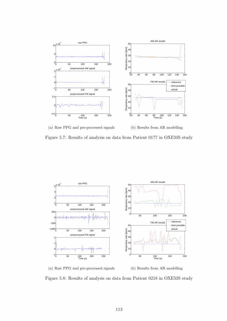
0 50 100 150 2000

5

10x 10

4 raw PPG

0 50 100 150 200−1

0

1

2x 10

4 preprocessed AM signal

0 50 100 150 200−0.5

0

0.5preprocessed FM signal

Time (s)

(a) Raw PPG and pre-processed signals

20 40 60 80 100 120 140 1600

10

20

30

40

50AM AR results

Res

pira

tory

rat

e (b

pm)

20 40 60 80 100 120 140 1600

10

20

30

40

50FM AR results

Time (s)

Res

pira

tory

rat

e (b

pm)

reference

best possible

actual

(b) Results from AR modelling

Figure 5.7: Results of analysis on data from Patient 0177 in OXEMS study

0 50 100 150 2002

3

4

5x 10

4 raw PPG

0 50 100 150 200−1000

−500

0

500preprocessed AM signal

0 50 100 150 200−1

0

1

2preprocessed FM signal

Time (s)

(a) Raw PPG and pre-processed signals

50 100 150 2000

10

20

30

40

50AM AR results

Res

pira

tory

rat

e (b

pm)

50 100 150 2000

10

20

30

40

50FM AR results

Time (s)

Res

pira

tory

rat

e (b

pm)

reference

best possible

actual

(b) Results from AR modelling

Figure 5.8: Results of analysis on data from Patient 0218 in OXEMS study

113

rate (similar to that seen in Figure 5.7) in the results from at least one AR method. In

addition, a further nine records showed results of similar quality to that seen in Figure 5.8,

where it is conceivable that a reasonable estimate of respiratory rate could be extracted

from the results. Many of the remaining records had short periods of good accuracy

with one or more of the AR methods, although a few showed very poor performance,

as demonstrated in Figure 5.9. As with the results of the Oxford School study, the

comparison of the best possible poles to the reference respiratory rate showed that it was

theoretically possible to obtain high accuracy from both AM and FM methods in almost

all cases. However, it was observed that these poles frequently had low magnitude, making

it unlikely that they would be chosen as the breathing pole, and indicating that although

the respiratory signal was present, it had low spectral power in comparison to other signals

in the frequency range of interest.

0 20 40 60 80 100 1200

5

10x 10

4 raw PPG

0 20 40 60 80 100 120−2

0

2x 10

4 preprocessed AM signal

0 20 40 60 80 100 120−1

0

1

2preprocessed FM signal

Time (s)

(a) Raw PPG and pre-processed signals

30 40 50 60 70 80 90 1000

10

20

30

40

50

60AM AR results

Res

pira

tory

rat

e (b

pm)

reference

best possible

actual

30 40 50 60 70 80 90 1000

10

20

30

40

50

60FM AR results

Time (s)

Res

pira

tory

rat

e (b

pm)

(b) Results from AR modelling

Figure 5.9: Results of analysis on data from Patient 0162 in OXEMS study

Unlike the children enrolled in the Oxford School study, the children whose vital signs

were measured in the OXEMS study were all sufficiently unwell to require a consultation

at the out-of-hours GP surgery. The OXEMS surgery is not a walk-in surgery, but requires

patients to go through a telephone-based triage system with one of the on-call doctors

before attending the surgery. It can therefore be assumed that all of the children in the

study were unwell, or showing symptoms that made a doctor believe that further urgent

114

investigation was necessary. This information provides some explanation for the poor

performance of the AR methods, as discussed below.

Illness is known to reduce the strength of respiratory sinus arrhythmia (van Ravenswaaij-

Arts et al., 1993), and it is likely that this mechanism was present for some of the children

in the OXEMS study. In addition, as previously discussed, respiratory sinus arrhythmia

is strongest at low respiratory rates, which were infrequently seen in the children in the

OXEMS study. This was due in part to the age profile of the children, who had a median

age of 2.8 years, and so would be expected to have high resting respiratory rates. These

rates would also tend to increase further in the presence of illness, resulting in even higher

rates, and consequently lower levels of respiratory sinus arrhythmia. Children with respi-

ratory illness may also have shown signs of recession or use of accessory muscles, which

could have reduced the strength of the AM modulation of the PPG waveform.

In addition to these specific issues, it is also likely that both AR methods suffered

from interference due to movement artefact and resulting poor signal quality. Many of

the children in the OXEMS study were under school age, and while the research nurse

did not note significant problems with the acceptability of the finger probe, it was noted

that many children were restless and unable to keep the measurement site still for the

length of the recording. However, it is clear from comparison of the raw PPG signals that

the level of artefact on the data from the OXEMS study is less than that in the Oxford

School study, and this may in part explain the better accuracy seen in the data from the

OXEMS study.

A further difficultly with interpretation of the results of the OXEMS study comes from

potential problems with the accuracy of the manual respiratory rate measurement. In the

protocol for the study, it was stated that the manual measurement would be made over 60

seconds. However, inspection of the recorded respiratory rates showed that they were all

even numbers, and that all rates greater than 56 breaths/minute were exactly divisible by

4. It was therefore hypothesised that respiratory rates were measured over 30 seconds and

doubled, and that high rates were measured over 15 seconds and multiplied by four. This

introduced additional error in the estimate of the reference respiratory rate, which may

have been inaccurate by up to 4 breaths/minute for children measured over 30 seconds,

115

or 8 breaths/minute at high respiratory rates, where it appears that measurements were

made over 15 seconds.

Kalman filtering of results from the OXEMS study

A number of the records in the OXEMS study showed generally good accuracy in the

respiratory rate calculated using the pole-choice algorithm described in Section 5.2.2, but

with occasional ‘spikes’, where the AR method failed to track the respiratory rate in a

particular window. As Kalman filtering had been shown to be effective when applied to

results containing similar artefacts in the AR-derived respiratory rate from the PPG in

adults, a similar method was tested on the data from the OXEMS study.

The parameters for the Kalman filter were derived from the statistics of the OXEMS

data as described in Appendix B.4. Values for the initial state x0, and initial covariance

P0 were calculated from the expected value and variance of the reference respiratory rates

in the OXEMS data set. Since the reference rate in the OXEMS data is constant over

a given record, the process noise covariance Q was set to be 0. The measurement noise

covariance R was estimated for both AM and FM methods, and the covariance matrix

for each method was also estimated. Values of the estimated parameters were compared

to those calculated from the data in the Oxford School study. The only large difference

between the two studies was in the calculated value for P0, which was twice as large in

the OXEMS study (200 compared to 100), due to the larger variation in respiratory rate

observed in the OXEMS study subjects.

Equation 5.1 shows the Kalman parameter estimates for the state transition matrix

A, and the process noise covariance Q. The estimates of the initial values of the state x0

and covariance P0 are given in Equation 5.2. Values for the observation matrix H, and

the process noise covariance R are shown in Equation 5.3. As the estimated values for

R did not differ greatly between the two AR methods, it was decided that a single value

could be used for both.

A = 1, Q = 0 (5.1)

116

x0 = 30, P0 = 200 (5.2)

H = 1, R = 300 (5.3)

One-dimensional Kalman filters were run on the results of both AR methods for all 44

OXEMS study records under analysis. As the respiratory rate in the OXEMS study was

assumed to be constant, the last output of the Kalman filter was the most appropriate

estimator of the respiratory rate, as it took into account all previous measurements. The

error in respiratory rate was calculated as the absolute error between the final output

of the Kalman filter and the reference rate. As in Chapter 4, the errors were reported

in terms of the mean, and the 5th and 95th percentiles. The number of patients with

absolute errors less than 5 breaths/minute were also reported. It was felt that this level of

accuracy should be sufficient to detect significant tachypnoea or bradypnoea in children,

while taking into account the achievable level of accuracy given the potential errors in the

measurement of the reference respiratory rates.

10 20 30 40 50 60 70 800

20

40

60

80

100

120

140

Reference respiratory rate (breath/min)

Per

cent

age

erro

r

(a) AM results

10 20 30 40 50 60 70 800

10

20

30

40

50

60

70

80

90

Reference respiratory rate (breath/min)

Per

cent

age

erro

r

(b) FM results

Figure 5.10: Scatter plots of percentage error in estimated respiratory rate against thatreference rate. Note that the vertical scales differ between the two graphs.

The results in Tables 5.2 and 5.3 show that the mean error across the whole OXEMS

data set was high. The graphs in Figure 5.10 also show that there was a relationship

between the reference respiratory rate and the percentage error for estimates made using

both AM and FM techniques. Both methods appear to perform poorly at high respiratory

rates. This might be expected, as the most unwell children are likely to exhibit not only the

117

Patient ID Error using AM method Error using FM method(breaths/minute) (breaths/minute)

0122 10.4 19.70128 8.8 9.10130 21.8 4.20133 5.7 20.40137 7.2 12.20151 13.9 13.90154 4.5 22.00155 1.6 2.00161 13.0 5.70162 20.2 34.50164 0.6 6.30166 9.3 15.30168 3.3 6.10170 20.7 44.10172 16.9 1.00174 2.5 2.30175 13.3 4.20176 11.4 1.80177 1.8 3.10178 7.9 2.20179 1.8 2.90188 0.8 12.60191 11.6 1.20193 11.3 3.10196 6.5 6.50199 14.5 10.10200 15.9 16.00201 5.6 22.10204 0.7 18.70211 34.0 34.00215 15.8 4.80216 11.8 8.50217 16.7 8.00218 23.0 6.90219 6.0 6.00222 39.4 55.60229 0.5 16.30231 8.2 5.60232 17.4 31.10235 12.0 25.90240 7.4 22.60242 2.0 2.00244 3.0 1.60248 24.2 32.9

Table 5.2: Absolute error of Kalman filtered AR-derived respiratory rates for patients inthe OXEMS study. Errors of less than 5 breaths/minute are emboldened.

118

Kalman filter Mean error (5–95%) Error < 5 breaths/minute(breaths/minute) (patients)

AM 11.0 (0.67–27.1) 12FM 13.3 (1.52–37.4) 14

Table 5.3: Results from Kalman filtering of AR-derived respiratory rates using data fromthe OXEMS study

highest respiratory rates, but are also most likely to have low levels of heart rate variation,

and increased accessory muscle use, which would be expected to reduce the accuracy of

both methods. The loss of accuracy at high rates is particularly noticeable in the FM

data, and may be due to the reduction in the strength of respiratory sinus arrhythmia at

high respiratory rates. Both Nemati et al. (2010) and Kuan (2010) observed moderate

increases in accuracy with respiratory rate, but these studies were confined to normal

adult respiratory rates of below 30 breaths/minute, whereas the increase in error with

respiratory rate in the OXEMS data is only noticeable at higher rates. Indeed, if only

rates up to 30 breaths/minute are considered, the AM method on the OXEMS data also

appears to show increased accuracy with increasing respiratory rate.

For each method, around a quarter of the 44 patients had an absolute error in res-

piratory rate less than 5 breaths/minute. Further investigation showed that six patients

(14%) showed this level of accuracy in the results from all both Kalman filters, indicating

that accurate respiratory rate could almost certainly be calculated for these patients. In

addition, a further 14 patients (32%) showed this accuracy in the results from at least

one Kalman filter. The remaining 24 patients showed poor accuracy in the results from

both AM and FM Kalman filters, and it is unlikely that accurate respiratory rates could

be derived from these patients using the AR methods presented in this section.

5.4 Assessment of PPG signal quality

Just under half of the records (45%) from the OXEMS study showed adequate accuracy

in predicting respiratory rate using Kalman filtering with at least one of the AR methods.

It was hypothesised that poor PPG signal quality was a major cause of poor accuracy in

predicting respiratory rate, due to excessive noise and artefact on the recorded waveform.

A wide variety of noise sources may lead to poor PPG signal quality. Correct probe

119

positioning, and choice of an appropriately sized probe, are important to ensure that noise

and artefacts are kept to a minimum. In the OXEMS study, three different probe sizes

were available to allow for the different sizes of enrolled children, but it is possible that

the most appropriate probe was not always selected. Inappropriate probe choice may lead

to increased levels of motion artefact and intrusion of ambient light, particularly if the

probe is too large.

Motion artefact is a particular challenge when collecting data from children, who may

be unwilling or unable to remain still during the monitoring period. Use of adhesive

probes, which are less likely to be dislodged during motion, may reduce the effect of

motion artefact, but are unlikely to completely eliminate it. In the OXEMS study, clip

probes were used for most children, with adhesive probes only being applied to infants.

While clip probes are quicker and easier to apply, they are more prone to slip on the

finger, which may lead to noise, artefactual signals, or even complete loss of signal, if the

finger moves out of the light path. Such problems are more likely if the probe is too large,

or if the patient is moving.

In addition to these causes of poor signal quality, the strength of the breathing signal

(AM or FM) in the PPG waveform may be affected by a variety of physiological factors,

as previously discussed. Shallow breathing, or use of accessory muscles, may reduce the

AM signal, and a number of disease processes reduce the strength of respiratory sinus

arrhythmia, which is responsible for the FM signal. All of these potential confounding

situations are likely to be more common in unwell children, further complicating the

detection of respiratory rate in this population.

If periods of poor signal quality, or correlates of poor respiratory modulation of the

PPG waveform, could be detected, it might be possible to use this data to improve

estimations of respiratory rate. This could be achieved by rejecting poor quality data, or

reducing its influence on the final reported estimate. In addition, a real-time indication of

signal quality could be used to alert the user, allowing them to adjust the siting or fit of

the probe in order to obtain a better signal. Existing pulse oximeters frequently provide

an indication of signal quality to ensure that SpO2 and heart rate can be accurately

reported. However, these indications may not be sufficiently sensitive to alert users to

120

issues that would affect the estimation of respiratory rate.

The oximeter used in this study gave some indication of poor signal quality by report-

ing invalid heart rate or SpO2, and this was used to discard sections of PPG from the

analysis, as described in Section 5.2.1. However, this information was insufficient to iden-

tify all periods of poor signal quality that affected the calculation of accurate respiratory

rates.

Gil et al. (2008) report the use of Hjorth parameters to identify artefacts on PPG

waveforms recorded from adults and children during sleep studies. An initial investigation

was therefore carried out to ascertain whether Hjorth parameters could be used to identify

data that would result in inaccurate estimates of PPG-derived respiratory rate. Hjorth

parameter values were calculated based on both the raw PPG, and the pre-processed data

prior to AR modelling, but did not correlate with error rates in the estimated respiratory

rate. Since Gil et al. (2008) were not calculating respiratory rates from the PPG, but

rather were attempting to identify periods of apnoea (cessation of breathing), it is possible

that this signal quality assessment was unable to identify morphologies or artefacts in the

PPG signal that would adversely affect the calculation of respiratory rate, but would not

affect the identification of apnoea.

Strachan (2010) developed an alternative signal quality assessment using probabilistic

principal component analysis (PPCA) and extreme value theory. This method had been

developed on adult PPG data, with the intention of identifying periods of poor quality

signal that would lead to inaccurate estimations of respiratory rate using AR modelling

techniques. As this technique had showed promise in a similar domain, it was applied to

the OXEMS data, using a subset of the Oxford School study dataset as an independent

training set.

A variety of methods have been proposed for signal quality assessment of other pul-

satile waveforms, such as the ECG, and the arterial blood pressure waveform. Moody and

Mark (1989) use feature vectors derived using the Karhunen-Loeve transform to quantify

noise on ECG waveforms. This method has similarities to the PPCA method devel-

oped by Strachan (2010), which uses similarly derived feature vectors to define ‘normal’

morphology. Zong et al. (2004) and Sun et al. (2006) both use heuristic measures to iden-

121

tify physiologically implausible artefacts and noise in arterial blood pressure waveforms.

These heuristics can be combined using fuzzy logic to obtain a continuous measure of

signal quality (Zong et al., 2004), or using the OR operator to give a dichotomous mea-

sure (Sun et al., 2006). Li et al. (2009) combines these two approaches by using the

fuzzy logic method proposed by Zong et al. (2004), but with an additional dichotomous

index calculated using the AND operator to modify the index in the presence of multiple

physiologically implausible measures. Li et al. (2008) use multiple indices to identify poor

quality ECG waveforms, including assessing the correlation of different beat detectors and

detection of beats on different ECG leads. They also use knowledge of the properties of

good quality waveforms to identify noise and artefacts by changes in the kurtosis and fre-

quency spectrum of the signal. Due to time constraints, it was not possible to investigate

these methods further in this thesis.

5.4.1 Training the model for PPCA novelty analysis

The mathematical basis of PPCA is described in Appendix B.5. To assess the signal

quality of the PPG, the PPCA model was trained using shape vectors from the PPG

waveform, with each shape vector representing a section of the waveform between two

salient points (defined in the same manner as when deriving salient points for FM pre-

processing).

The salient points in the PPG waveform were used to split the waveform up into

sections. Each of these sections was then interpolated using linear interpolation to obtain

a shape vector with 50 evenly sampled points. This vector was transformed to have a

minimum value equal to zero and an area under the curve equal to one. This process

is demonstrated in Figure 5.11. All of the sections of the original PPG waveform were

treated in the same way to obtain a series of ‘shape vectors’, which were used as a 50-

dimensional input for training the PPCA model as described in Appendix B.5.

The PPCA model was trained using the PPG waveforms from four records from the

Oxford School study. As the intention was to use PPCA to predict which PPG sections

would result in good-quality respiratory rate extracted from AR modelling, the records for

the training set were chosen to be those which showed the best accuracy in the prediction

122

10 12 14 16 18 20−2000

−1500

−1000

−500

0

500

Time (s)

PP

G

0 50−1500

−1000

−500

0

500

Sample

Res

ampl

ed

0 500

0.01

0.02

0.03

0.04

0.05

Sample

Tra

nsfo

rmed

Figure 5.11: Detection and pre-processing of shape vectors for PPCA

of the respiratory rate using AR modelling. A PPCA model trained on a subset of the

OXEMS data set was also assessed, and was shown to produce similar results to that of the

model trained on data from the Oxford School Study. By using the Oxford School study

data to train the PPCA model, the whole of the OXEMS study data could be treated

as an independent test set. In addition, since the two studies used different oximeter

devices1, this also confirmed that a new PPCA model should not be required to assess

data acquired with different oximeter devices. Although the heart rate may have some

effect on the shape of the waveform, the variety of heart rates in the data from the Oxford

School Study should ensure that this variation was captured in the training data.

Training of the PPCA model was carried out in two steps, to reduce the effect of

outlier shape vectors. In the first step, the shape vectors were normalised so that each

of the 50 dimensions had zero mean and unit variance. Eigenvalue decomposition of the

shape vectors was then carried out, and the number of principal components, p, was

defined as the number of eigenvalues that explained 98% of the total variance (i.e. the

number of dominant eigenvalues such that the cumulative sum was greater than 98% of the

total sum). The 50-dimensional shape vectors were then mapped into the p-dimensional

space defined by the corresponding eigenvectors using Equation B.19. The transformed p-

dimensional data was then subject to pruning using Gaussian mixture models as described

in Appendix B.7, with the probability cut-offs for model inclusion and data inclusion

selected to be 0.8 and 0.9 respectively.

In the second step, the pruned data was removed from the set of shape vectors, and

1The Visi-3 system used for the Oxford School study uses Masimo oximetry, whereas a Nonin pulseoximeter was used for the OXEMS study

123

normalisation and eigenvalue decomposition carried out again as described above. As

before, the number of principal components was defined to be the number of eigenvalues

that accounted for 98% of the total variance. The PPCA model was then built using the

pruned set of shape vectors as described in Appendix B.5. Training the PPCA model

using the four records from the Oxford School study resulted in a final PPCA model with

9 principal components.

The PPCA model defines a unimodal, multivariate Gaussian probability density func-

tion. The extreme value theory methods described in Appendix B.6 and Clifton et al.

(2010) can then be applied to this distribution. The PPCA model is equivalent to the

distribution fn(x) in Equation B.26, with dimensionality n = p. To calculate the scale

and shape parameters in Equations B.33 and B.34, we used m = 50, as the shape vectors

each contained 50 points.

Once the model had been trained as described above, novelty scores could be computed

for test PPG data. To do this, shape vectors were identified by the position of salient

points, and interpolated to be 50 samples in length. As before, the shape vectors were

pre-processed to ensure a minimum value of zero, and an area under the curve of one. The

resulting shape vectors were then normalised using the means and standard deviations

calculated from the pruned training dataset, to ensure that each element of the shape

vector had equal importance. The novelty score for the shape vectors was then calculated

by extreme value theory using Equation B.35 in Appendix B.6.

5.4.2 Results on data from the OXEMS study

Novelty analysis was applied to the PPG waveforms for the 44 records in the OXEMS

data set. For each portion of waveform between two detected salient points, a novelty

score was returned, ranging from 0 to 36, with this upper limit determined by the machine

precision of the computer.

Figures 5.12 and 5.13 show examples of the novelty values for two patients in the

OXEMS study. These show that high values of novelty typically occur around areas of

the PPG waveform where the waveform appears to contain artefacts (e.g. at around 70

seconds in Figure 5.12). Areas of high novelty were often clustered, supporting the theory

124

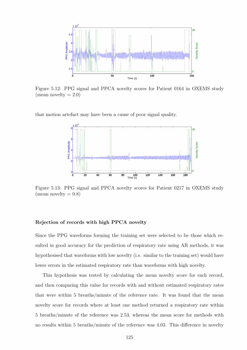
0 50 100 150

2.5

3

3.5

4

4.5

x 104

Time (s)

PP

G A

mpl

itude

0 50 100 150

0

36

Nov

elty

Sco

re

Figure 5.12: PPG signal and PPCA novelty scores for Patient 0164 in OXEMS study(mean novelty = 2.0)

that motion artefact may have been a cause of poor signal quality.

0 20 40 60 80 100 120 140 160 1802

3

4

5

6x 10

4

Time (s)

PP

G A

mpl

itude

0 20 40 60 80 100 120 140 160 180

0

36

Nov

elty

Sco

re

Figure 5.13: PPG signal and PPCA novelty scores for Patient 0217 in OXEMS study(mean novelty = 0.8)

Rejection of records with high PPCA novelty

Since the PPG waveforms forming the training set were selected to be those which re-

sulted in good accuracy for the prediction of respiratory rate using AR methods, it was

hypothesised that waveforms with low novelty (i.e. similar to the training set) would have

lower errors in the estimated respiratory rate than waveforms with high novelty.

This hypothesis was tested by calculating the mean novelty score for each record,

and then comparing this value for records with and without estimated respiratory rates

that were within 5 breaths/minute of the reference rate. It was found that the mean

novelty score for records where at least one method returned a respiratory rate within

5 breaths/minute of the reference was 2.53, whereas the mean score for methods with

no results within 5 breaths/minute of the reference was 4.03. This difference in novelty

125

0 5 10 150

10

20

30

40

Mean novelty

Err

or (

brea

ths/

min

ute)

(a) AM results

0 5 10 150

10

20

30

40

50

60

Mean novelty

Err

or (

brea

ths/

min

ute)

(b) FM results

Figure 5.14: Mean novelty scores for records from the OXEMS study compared to absoluteerror in estimated respiratory rate from AM and FM autoregressive modelling. Recordsrejected on the basis of mean novelty score are shown in red.

score was shown to be statistically significant (P=0.043) using a single-tailed Student’s

t-test. It was noted that a threshold of 6 on the mean PPCA novelty score would identify

8 of the 24 poorly-performing records (33%), and retain all of the 20 better-performing

records, as can be seen in Figure 5.14. It was therefore decided that a threshold of 6 on

the novelty score would be used to reject poor quality records.

Kalman filtering using PPCA novelty scores

In addition to applying a record-wide rejection threshold to the data from the OXEMS

study, the PPCA novelty scores were investigated to determine whether they could im-

prove the performance of the Kalman filtering. This was carried out by modifying the R

matrix for each window, so that measurements obtained from windows with low novelty

would have a greater influence on the estimator than measurements from windows with

high novelty.

A novelty score was calculated for each section of the waveform between two salient

points, so each 60-second window corresponding to an estimated respiratory rate had

multiple novelty scores. As a short interval of poor-quality PPG signal could have a large

effect on the AR model for the window, it was decided that the most appropriate metric

for assessing the quality within a given window should be the maximum novelty score

within that window. This metric resulted in most windows having a score equal to either

the maximum or minimum novelty scores, with only a minority of windows having novel

126

sections without an associated maximum novelty score, as can be seen in Figure 5.15.

0 10 20 30 400

10

20

30

40

50

60

Maximum novelty within window

Err

or fo

r w

indo

w (

brea

ths/

min

ute)

(a) AM results

0 10 20 30 400

20

40

60

80

Maximum novelty within window

Err

or fo

r w

indo

w (

brea

ths/

min

ute)

(b) FM results

Figure 5.15: Maximum novelty score and absolute error in respiratory rate for windowsin the OXEMS dataset. Windows from records excluded on the basis of mean noveltyscore are not shown.

The measurement noise covariance, R, was estimated from the measurement errors in

each window. Windows were separated into three groups by the value of the maximum

novelty score. Since the majority of windows had a maximum novelty score equal either

to the minimum or maximum possible values as shown in Figure 5.15, windows with

intermediate scores were combined into one group, as it was not felt that there was

sufficient information on intermediate scores to employ a method similar to that used by

Li et al. (2008), where R varies continuously with signal quality. These estimated values

are presented in Equations 5.4–5.6. In these equations, the subscripts n ≤ 0, 0 < n ≤ 36,

and n > 36 identify which value of R was used for a window with a maximum novelty

score of n.

Rn≤0 = 100 (5.4)

R0<n≤36 = 150 (5.5)

Rn>36 = 350 (5.6)

As in the previous section, Kalman filters were applied to the outputs of both AR

methods. However, the results in Table 5.5 only show the results from the 36 records

127

Patient Mean PPCA Error using AM method Error using FM methodID novelty score no PPCA PPCA no PPCA PPCA

Kalman Kalman0122 4.0 10.4 10.4 19.7 19.40128 0.4 8.8 8.6 9.1 8.60130 1.9 21.8 21.3 4.2 4.50133 4.1 5.7 5.8 20.4 20.30137 0.5 7.2 5.1 12.2 11.70151 13.3 13.9 13.9 13.9 13.90154 3.8 4.5 4.6 22.0 22.00155 3.4 1.6 1.6 2.0 1.90161 1.0 13.0 14.7 5.7 6.20162 2.2 20.2 20.2 34.5 34.30164 2.0 0.6 5.4 6.3 6.40166 3.3 9.3 9.0 15.3 14.70168 3.2 3.3 3.4 6.1 6.20170 1.3 20.7 17.3 44.1 42.90172 3.2 16.9 15.1 1.0 0.50174 0.3 2.5 2.8 2.3 1.90175 0.9 13.3 13.6 4.2 4.40176 0.8 11.4 10.8 1.8 1.00177 0.7 1.8 0.6 3.1 2.60178 1.1 7.9 2.9 2.2 1.80179 0.2 1.8 1.6 2.9 2.70188 1.5 0.8 0.2 12.6 11.90191 0.9 11.6 12.1 1.2 0.010193 1.1 11.3 11.5 3.1 3.00196 5.5 6.5 6.5 6.5 6.50199 2.3 14.5 14.3 10.1 9.90200 6.1 15.9 15.5 16.0 15.50201 8.5 5.6 5.6 22.1 21.90204 3.4 0.7 0.8 18.7 18.50211 7.0 34.0 34.0 34.0 34.00215 5.5 15.8 15.3 4.8 4.30216 2.4 11.8 8.3 8.5 10.80217 0.8 16.7 19.0 8.0 6.50218 2.5 23.0 22.6 6.9 6.50219 7.2 6.0 6.0 6.0 6.00222 2.2 39.4 39.4 55.6 55.50229 5.0 0.5 0.7 16.3 15.60231 0.4 8.2 7.4 5.6 6.20232 3.9 17.4 17.8 31.1 30.80235 6.3 12.0 12.0 25.9 25.80240 9.1 7.4 7.4 22.6 22.10242 3.3 2.0 2.0 2.0 2.00244 2.1 3.0 3.0 1.6 1.90248 8.7 24.2 24.3 32.9 32.7

Table 5.4: Absolute error (breaths/minute) of AR-derived respiratory rates calculatedwith and without PPCA-assisted Kalman filtering for patients in the OXEMS study.Errors of less than 5 breaths/minute are emboldened, and patients with a mean PPCAnovelty score of greater than 6 are italicised.

128

which had a mean novelty score of less than 6, as 8 records were rejected on the basis

of the mean novelty score (shown in italics in Table 5.4). Comparing these results with

those in Table 5.3 shows that using PPCA-derived novelty scores to reject extremely

poor quality records, and to assist the Kalman filtering, resulted in an improvement of

approximately 1.5 breaths/minute in the mean error for each method.

Kalman filter Mean error (5–95%) Error < 5 breaths/minute(breaths/minute) (patients)

AM 9.9 (0.64–22.2) 12FM 11.2 (0.66–40.4) 14

Table 5.5: Results from PPCA-assisted Kalman filtering of AR-derived respiratory ratesusing data from the OXEMS study

PPCA-assisted Kalman filtering rejected 8 out of 44 records (18%), and resulted in at

least one method producing a respiratory rate within 5 breaths/minute of the reference

rate in 20 of the remaining 36 records (55%).

Removal of poor-quality PPG data using PPCA novelty scores

The PPCA novelty scores calculated for the OXEMS data were also used to remove poor-

quality sections of the PPG waveform prior to AR modelling. It was hypothesised that the

removal of these sections of waveform would reduce the influence of dominant poles due

to short-lived artefacts on the PPG waveform. This method was therefore implemented

in addition to the record-wide rejection threshold discussed previously.

As can be seen from Figures 5.12 and 5.13, the majority of shape vectors were allocated

a novelty score less than or equal to 0. It was therefore decided that all sections of

PPG waveform with a novelty score higher than 0 would be removed from the analysis.

For each window, sections of PPG waveform with high novelty were removed, and the

remaining sections spliced together to form a shorter waveform containing only low-novelty

data. No padding was introduced, and the spliced waveform was not processed to remove

discontinuities, although such processing may be worthy of further investigation in the

future to improve the accuracy of this method.

AR modelling was carried out to estimate the respiratory rate using both AM and FM

methods, with the analysis being carried out using only sections of the PPG waveform

with low novelty. Kalman filtering was carried out on the results of this analysis, using

129

the parameters specified in Section 5.3.2. The results of this analysis are shown in Tables

5.6 and 5.7. The results in Table 5.7 refer only to the 36 records that were not removed

based on their mean novelty score.

Removal of high-novelty sections of the PPG waveform prior to AR modelling produced

more accurate estimations of respiratory rate than PPCA-assisted Kalman filtering, with

an additional four patients having an estimated respiratory rate within 5 breaths/minute

of the reference rate. Out of the original 44 records, 8 (18%) were rejected on the basis

of their mean PPCA novelty score, and of the remaining 36 records, 24 (66%) produced

an estimated respiratory rate accurate to within 5 breaths/minute for at least one AR

method, corresponding to 55% of the original 44 records.

However, 17 of these records achieved this level of accuracy using only one of the two

AR methods. There is therefore a further level of complexity in identifying the accurate

result in each case, which will not be investigated in this thesis. In 7 records, the accuracy

was greater than 5 breaths/minute for both methods, and so a simple combination of the

results would be sufficient to obtain an accurate estimate of respiratory rate.

5.5 Summary

It is hypothesised that motion artefact on the PPG waveform was responsible for much

of the poor signal quality observed during this investigation. This hypothesis is based on

observation of the artefact morphology in the PPG waveform, and also from feedback from

the research nurse who carried out the data collection, who observed that many children

were unable to remain still for the two-minute data collection period. Young children do

not tend to remain still for long periods of time unless they are asleep or seriously ill, and

so motion artefact is likely to remain a major problem for investigations involving the

PPG in paediatric populations. Using a measure of signal quality, such as PPCA novelty

scores, to identify and remove sections of poor-quality PPG waveform prior to analysis

provides some mitigation for this problem, but is not effective in every situation.

Some records did not show obvious motion artefacts, but still performed very poorly

when trying to extract the respiratory rate using AR modelling. There are a number of

possible reasons for this. It is possible that the pulse oximeter probe was not correctly

130

Patient Mean PPCA Error using AM method Error using FM methodID novelty score no PPCA PPCA no PPCA PPCA

removal removal0122 4.0 10.4 2.0 19.7 20.30128 0.4 8.8 6.8 9.1 8.20130 1.9 21.8 12.0 4.2 1.50133 4.1 5.7 7.0 20.4 26.70137 0.5 7.2 8.2 12.2 11.60151 13.3 13.9 13.9 13.9 13.90154 3.8 4.5 3.0 22.0 19.50155 3.4 1.6 3.5 2.0 5.90161 1.0 13.0 10.7 5.7 2.60162 2.2 20.2 34.4 34.5 35.20164 2.0 0.6 8.9 6.3 5.30166 3.3 9.3 9.2 15.3 4.60168 3.2 3.3 4.4 6.1 4.60170 1.3 20.7 18.3 44.1 44.00172 3.2 16.9 21.2 1.0 0.20174 0.3 2.5 0.8 2.3 1.50175 0.9 13.3 11.7 4.2 3.40176 0.8 11.4 13.2 1.8 0.80177 0.7 1.8 0.2 3.1 2.90178 1.1 7.9 2.1 2.2 1.10179 0.2 1.8 1.7 2.9 2.40188 1.5 0.8 8.6 12.6 4.60191 0.9 11.6 9.5 1.2 10.50193 1.1 11.3 14.9 3.1 1.00196 5.5 6.5 6.5 6.5 6.50199 2.3 14.5 0.8 10.1 10.60200 6.1 15.9 10.6 16.0 14.40201 8.5 5.6 0.5 22.1 28.10204 3.4 0.7 2.8 18.7 18.60211 7.0 34.0 34.0 34.0 34.00215 5.5 15.8 2.5 4.8 2.30216 2.4 11.8 5.8 8.5 10.70217 0.8 16.7 11.7 8.0 5.40218 2.5 23.0 16.2 6.9 1.70219 7.2 6.0 6.0 6.0 6.00222 2.2 39.4 35.4 55.6 56.40229 5.0 0.5 4.2 16.3 5.50231 0.4 8.2 7.5 5.6 4.10232 3.9 17.4 17.0 31.1 25.30235 6.3 12.0 11.3 25.9 32.10240 9.1 7.4 14.8 22.6 17.30242 3.3 2.0 2.0 2.0 2.00244 2.1 3.0 5.8 1.6 0.60248 8.7 24.2 12.8 32.9 35.5

Table 5.6: Absolute error (breaths/minute) of AR-derived respiratory rates calculatedwith and without removal of PPG sections based on the PPCA novelty score for patientsin the OXEMS study. Errors of less than 5 breaths/minute are emboldened, and patientswith a mean PPCA novelty score of greater than 6 are italicised.

131

AR method Mean error (5–95%) Error < 5 breaths/minute(breaths/minute) (patients)

AM 9.2 (0.81–30.5) 13FM 10.2 (0.66–41.4) 18

Table 5.7: Results from AR-derived respiratory rate estimation using only low-noveltysections of the PPG waveforms from the OXEMS study

applied to the child’s finger, resulting in a poor-quality signal without enough informa-

tion about peripheral blood flow to allow estimation of the respiratory rate. It is also

possible that some of the children had illnesses or pre-existing conditions which affected

the physiological processes which result in AM or FM modulation of the PPG waveform.

It is known that a number of conditions, as well as high respiratory rates, are capable of

suppressing respiratory sinus arrhythmia, and it is hypothesised that shallow breathing,

recession, or the use of accessory muscles may reduce the amplitude modulation of the

PPG by reducing the variation in thoracic pressure during the breathing cycle.

The results in this chapter have shown that it is possible to use AR modelling to

estimate accurate respiratory rates for children monitored in primary care. However,

obtaining sufficient quantities of clean data from unwell children is a challenge, as they do

not tend to remain still for the duration of the recording period. This results in motion

artefact on the PPG, which can make obtaining an accurate estimation of respiratory rate

difficult, or even impossible.

By using a PPCA-based novelty scores to remove sections of poor-quality PPG wave-

form, it has been possible to use AR models to estimate respiratory rates within 5

breaths/minute of the reference rate in 55% of the records in the OXEMS study. This

level of accuracy reflects both the believed accuracy of the reference rate, and the likely

error that would be acceptable in clinical practice.

The improvements in respiratory estimation obtained by implementing a signal quality

metric were predominantly due to the identification of a number of records with extremely

poor quality signals, which were then excluded from later analysis. Using the PPCA-

based novelty scores to assist with respiratory rate estimation in the remaining records

did lead to an overall improvement in the error for the OXEMS dataset, but this was not

always the case for an individual record. Further investigation is required to improve the

identification of poor-quality sections of waveform.

132

Chapter 6

Data fusion models for paediatric

triage

To obtain a single measure of the severity of illness from multiple sources of vital sign data,

it is necessary to use data fusion techniques. This chapter discusses the mathematical

basis of a number of different data fusion methods, and compares them using vital sign

data acquired from children in primary care. The resulting models are also compared to

cut-down versions of the PAWS scoring system (Egdell et al., 2008) using the same vital

sign data.

There are both advantages and disadvantages to assessing data fusion methods using

data collected in primary care. Primary care data should represent the spectrum of vital

signs (both normal and abnormal) that are encountered in this setting, and will also

contain a realistic mix of illness severities and ages (e.g. consultation is more common at

younger ages, and so these children will make up a higher proportion of the data set). In

addition, measurement techniques will be representative of those used in primary care.

More accurate results might be possible if data was collected from a population with a

higher level of acuity (for example, children who have been hospitalised). It is likely that

data collected in such settings would have fewer missing variables, such as respiratory

rate, as such measurement may be mandated, or may be more likely to be recorded due

to the perception of increased utility of this data in children who are more unwell. The

data may also have been measured using more accurate techniques, reducing the influence

of measurement error. However, there would be less coverage of children exhibiting vital

133

signs corresponding to low levels of acuity, which are common in primary care settings,

and the available outcome measures may not be directly applicable to the primary care

setting. As the intention of this study was to develop a data fusion method that could

be used to assist the triage of children in primary care, it was felt that good coverage of

the lower levels of acuity was important, and so only data collected from primary and

emergency care settings were considered.

The tests in this chapter were carried out using two vital signs datasets: Fever and

Tachycardia (FaT), and Walsgrave. These data sets were collected from children in pri-

mary and emergency care settings, and include binary outcome variables denoting whether

or not the child was considered to have a serious illness. The FaT dataset was collected

from feverish children attending primary care, with the classification of severity being

defined as hospital admission within a week of the assessment. In the Walsgrave study,

children attending a Paediatric Admission Unit with suspected acute infections were mon-

itored, and were classified based on the presence or absence of potentially life-threatening

infection. Further details of these vital signs datasets are given in Appendix A.2.

Appendix A.2 describes seven datasets derived from the FaT and Walsgrave data,

which are suitable for use in testing data fusion techniques. In this chapter, most of the

tests were carried out using the FaT3 dataset, which has a large sample size, although

it has a limited number of input variables and only a few serious cases; hence there is

not much data in the ‘abnormal’ class. The smaller Walsgrave3 dataset was selected as

an independent dataset to verify the results of the analysis carried out using the FaT3

dataset; the Walsgrave4 dataset was then used to investigate the benefit of including

respiratory rate as an extra input variable.

6.1 Data fusion methods

In this chapter, we consider data fusion methods which perform as classifiers. Thus,

we may train a model that classifies patients into those requiring hospital admission,

and those who are to be treated in the community. We then attempt to replicate this

classification by choosing an appropriate threshold on the data fusion output of the trained

classifier, with new patients being classified based on whether the data fusion output is

134

above or below the threshold.

This chapter considers two-class problems, with one class as the ‘abnormal’ class.

Children with more serious illness belong to this class, and it is typically the less likely

class. In clinical literature, the abnormal class is usually described as the ‘positive’ or

‘case’ class. The second class is referred to as the ‘normal’ class (not to be confused with

the normal, or Gaussian, distribution), and corresponds to the ‘negative’ or ‘control’ class

in the clinical literature.

True classificationNormal Abnormal

Normal True Negative False NegativeModel (Type I error)

Classification Abnormal False Positive True Positive(Type II error)

Table 6.1: Possible outcomes from classification

A binary classifier produces four types of results, as shown in Table 6.1. With real

data, it is necessary to make a compromise between the two types of error, as changing

the threshold to reduce one type of error will typically increase the incidence of the other

type. For a given threshold, the relative proportions of the different outcomes can be

described using sensitivity (Se) and specificity (Sp), which are defined in Equations 6.1

and 6.2.

Se =true positives

true positives + false negatives(6.1)

Sp =true negatives

true negatives + false positives(6.2)

The sensitivity is the proportion of positive patients who are correctly classified, and

the specificity is the proportion of negative patients who are correctly classified. A pair of

sensitivity and specificity values is only valid at a particular classifier threshold. The op-

timal threshold is usually determined using the Receiver Operating Characteristic (ROC)

curve, which plots Se against (1− Sp). The ROC curve always passes through the points

(0, 0) and (1, 1), which correspond to classifying all patients as negative or positive re-

spectively (Kirkwood and Sterne, 2003).

135

0 0.2 0.4 0.6 0.8 10

0.2

0.4

0.6

0.8

1

1−Specificity

Sen

sitiv

ity

Figure 6.1: ROC curve showing the sensitivity and specificity of using FEV1 measurementsfor predicting whether children in Peru would have respiratory symptoms (data fromKirkwood and Sterne (2003))

An example ROC curve is shown in Figure 6.1. The area under the ROC curve (AUC)

is a measure of the accuracy of the method. A perfect classifier will have an AUC of 1,

with the ROC curve following the x = 0 and y = 1 lines. The AUC is equivalent to

the probability that, given one randomly chosen positive case and one randomly chosen

negative case, the classifier will put them in the correct order. Therefore, an AUC of 0.5

corresponds to a classifier that performs no better than chance. The curve in Figure 6.1

has an AUC of 0.64, showing that the corresponding classifier has low accuracy.

The optimal threshold may be chosen by identifying the point on the ROC curve that

is closest to the (0, 1) point, as a perfect classifier will pass through the latter point.

Two-class classifiers are trained using both normal and abnormal data from the train-

ing dataset, and are optimised to separate out the data from the two classes. When there

are only a small number of examples from the abnormal class, the classification problem

may be considered from the perspective of novelty detection (sometimes termed one-class

classification). In novelty detection, a model of normality is constructed to fit the avail-

able normal data, and test data are identified as abnormal if they are novel with respect to

the trained model of normality. Novelty detection has previously been used to build data

fusion models for long-term physiological monitoring of adults (Tarassenko et al., 2005,

2006). In the examples used in this thesis, we have access to labelled data sets, but we

typically only have a small number of abnormal data points. It is therefore possible that

the abnormal data in our training dataset do not represent the full spectrum of possible

abnormal data. If this is the case, the novelty detection approach may be more successful

136

in identifying abnormal data in the test set.

Before training some of the data fusion models (e.g. Parzen windows), it is beneficial

to transform the variables (vital signs) in the training data set to have the same sam-

ple mean and variance. This ensures that there is equal weighting of each variable in

the model, and that the resulting distribution is independent of the units in which the

original measurements were made. The transformation is carried out by calculating the

sample mean µ and standard deviation σ of the training data, and then applying the

transformation in Equation 6.3 to the training data, where y is the original (untrans-

formed) data, and yt is the transformed data. Although it is only necessary for some

methods, this transformation was carried out in all cases, as it ensured consistency, and

was not detrimental to any method.

yt =y − µ

σ(6.3)

6.1.1 Two-class classifiers

Linear regression

A linear regression model (Kirkwood and Sterne, 2003) for data fusion can be built by

assigning an output value to each of the two classes (e.g. 1 and 0), and modelling this

output as a linear sum of the input variables. Equation 6.4 gives a linear regression

equation for three input variables: x1, x2, and x3.

y = β0 + β1x1 + β2x2 + β3x3 (6.4)

The four regression coefficients β0 to β3 are typically calculated using the least-squares

method on the training set (Kirkwood and Sterne, 2003), although other methods may

be used if the training set is expected to contain outliers which would skew the results.

Logistic regression

With two-class (binary) classifiers, it is often useful to consider the output value in terms

of the probability of observing one of the classes, p = yn, where p is the probability, y

137

is the output value for the class (1 or 0), and n is the number of identical data points

producing the output. Such an output value is naturally constrained to lie in the range

(0, 1), whereas the output from a standard linear regressor will not be so constrained,

leading to outputs which do not correspond to probabilities.

Logistic regression overcomes this problem by utilising a link function to transform the

output of the linear regressor, with a range of (−∞,∞), to a probability with a range of

(0, 1). The link function used in logistic regression is the logit function, shown in Equation

6.5.

logit(p) = ln

(p

1− p

)(6.5)

The equation for logistic regression is analogous to that for linear regression, except

that the output variable is now the transformed probability, as shown in Equation 6.6.

This equation also be re-written in the form shown in Equation 6.7.

logit(p) = β0 + β1x1 + β2x2 + . . . + βkxk (6.6)

p =y

n=

exp(β0 + β1x1 + . . . + βkxk)

1 + exp(β0 + β1x1 + . . . + βkxk)(6.7)

In the case of vital sign data, all of the input data xk are continuous, and therefore n =

1 always, so that yn

will always be exactly equal to 0 or 1, depending on the classification

of the data.

Gaussian mixture model classifiers

A Gaussian mixture model (GMM) (Bishop, 2006) uses a small number of Gaussian

kernels to model the probability distribution p(x) of a set of data. The general form of

such a model is given in Equation 6.8, where P (j) is the prior probability of the jth class,

and p(x|j) is the probability density of the jth kernel.

p(x) =k∑

j=1

P (j)p(x|j) (6.8)

The complexity of a GMM is set by the number of kernels k, and the form of the

138

covariance matrix (e.g. isotropic, diagonal, or full covariance).

The parameters of the GMM, θ, (priors, means and covariances) are set using the

expectation maximisation (EM) algorithm. The likelihood of the observed data with

respect to a given set of parameters is p(x|θ), and hence the likelihood of observing the

entire data set X = x1 . . .xN is given in Equation 6.9, where L(θ|X) is termed the

likelihood of the parameters given the data, or simply the likelihood.

p(X|θ) =N∏

i=1

p(xi|θ) = L(θ|X) (6.9)

We wish to find the set of parameters θ∗ that maximises L(θ|X), that is, the set of

parameters that are most likely to produce the observed data set. Typically, rather than

trying to maximise the likelihood, we try to maximise the log-likelihood: ln p(X|θ).When estimating the parameters of a mixture model, if we knew the labels Y =

y1 . . .yN denoting which component of the mixture generated each point in the dataset,

it would be relatively easy to calculate values for the priors, means and covariances of

each component. For example, the mean of each component could be estimated as the

sample mean of the data generated by that component.

Although we do not know the labels Y explicitly, we can incorporate them into our

definition of the likelihood function, such that the likelihood is defined as p(X,Y|θ). In

the E-step of the EM algorithm, we use the data and the current estimate of the GMM

parameters, θold, to find the expected value of the log-likelihood. This allows us to estimate

the distributions p(Y|X, θold), describing the likely values of the labels given the data and

the current estimate of the GMM parameters.

Given these labels, we can update our estimate of the GMM parameters to maximise

the likelihood of the observed dataset and obtain a new estimate of the GMM parameters

θnew. This is the M-step of the EM algorithm. These two steps are repeated until a

pre-determined termination criterion is met: typically convergence of θ to within a given

tolerance.

Since the EM algorithm is dependent on the initial estimate of θ, and is only guaranteed

to find a local minimum, it is sensible to train a number of GMMs on a given set of data,

and choose the one with the lowest error for testing.

139

To produce a GMM classifier, an independent GMM is built for each class, using the

data from that class. The values of k do not need to be equal for each class. To assess the

membership of a new data point xi, we calculate p(xi|j) for each class j, where each class

is represented by a GMM. For each class, the probability that xi belongs to the class is

given by Equation 6.10 (Bishop, 2006).

P (j|xi) =p(xi|j)P (j)

p(xi)(6.10)

For a two-class problem with equal priors P (j = 1) = P (j = 2), we can use the fact

that P (j = 1)|x)+P (j = 2|x) = 1 to calculate the values of P (j = 2|xi) without knowing

the value of p(xi). This results in Equation 6.11, which depends only on the values of

p(xi|j = 1) and p(xi|j = 2).

P (j = 2|xi) =p(xi|j = 2)

p(xi|j = 1) + p(xi|j = 2)(6.11)

6.1.2 One-class classifiers

Gaussian mixture models for novelty detection

In this instance, the model of normality is a Gaussian mixture model trained as described

in the previous section, using the normal data as the training set. As there is no abnormal

data in the training set, we cannot use Equation 6.11 to calculate the output of the model.

One option is to use the value of the probability density function p(xi) estimated by the

GMM at x = xi. This is acceptable for comparing outputs from the same model, but is

not valid for comparing outputs between GMM models of normality trained on different

data sets. The ability to compare the outputs from these models is important in the

experimental testing procedure used in this chapter, which uses a jack-knifing technique

to obtain ROC curves with a sufficient number of data points to assess the area under

the curve.

For comparing the outputs from different models, it is preferable to use a probability

rather than a probability density. Figure 6.2 shows how a probability at xi is derived

from the probability density function for 3 different values of xi. For a given value of xi,

140

0 10 20 30 40 500

0.01

0.02

0.03

0.04

0.05

0.06

p(x)

x

p(xi)

xi

P(p(x)>p(xi))

(a)

0 10 20 30 40 500

0.01

0.02

0.03

0.04

0.05

0.06

p(x)

x

p(xi)

xi

P(p(x)>p(xi))

(b)

0 10 20 30 40 500

0.01

0.02

0.03

0.04

0.05

0.06

p(x)

x

p(xi)

xi

P(p(x)>p(xi))

(c)

Figure 6.2: Calculating a probability at xi from the probability density function.

there is a corresponding value of p(xi), shown in the graphs as a dashed red line. The

probability calculated is the probability of drawing a point whose value of p(x) is greater

than p(xi) : P (p(x) > p(xi)). This probability is shaded in blue in the graphs in Figure

6.2. The probability will be small when xi is near the maximum of p(x), as demonstrated

in Figure 6.2(a), becoming large as xi reaches the tails of the distribution, as shown in

Figure 6.2(c). Therefore, a threshold, κ, on the probability P (p(x) > p(xi)) can be used

for novelty detection.

Parzen windows for novelty detection

The Parzen windows technique (Duda et al., 2001) estimates the probability density

function by placing a window function F (x) on each of the data points in a training

dataset. Each window function has an equal weight in the Parzen windows model, so that

the probability density at a given position xi is calculated using Equation 6.12. Provided

that the window function satisfies the constraints of a probability density function (non-

negative and integrating to one), the function calculated by the mean of the sums of the

window functions will also be a valid probability density function.

p(xi) = 1/NN∑

j=1

Fj(xi) (6.12)

In this thesis, we used an isotropic Gaussian as the window function for the Parzen

windows model, making the model a special case of the GMM. The window functions are

centred on the points, xj, in the training dataset, so that the mean of the jth Gaussian is

xj. The equation of the resulting probability density function is given in Equation 6.13,

141

where d is the dimensionality of the model (the number of variables).

p(x) =1

n

n∑

j=1

1

(2π)d/2σdexp

−|x− xj|2

2σ2

(6.13)

The variance σ2 is common to all of the window functions, and defines the smoothness

of the resulting probability density function. A large value of σ2 will result in wide

windows, and a smooth function, whereas a small σ2 will produce narrower windows, and

may result in over-fitting to the training data. It is therefore very important to calculate

an appropriate value for σ2.

A variety of methods have been suggested for calculating σ2. Bishop (1994) suggests

using the distance to the m nearest neighbours to set σ2. For each point in the training

dataset, the mean squared distance to the nearest m neighbours is calculated to give an

estimate of the local variance. The global variance is then calculated as the mean of these

local variances. In this chapter, we tested the performance of the model with different

values of m, and also used the maximum distance between centres to set σ2.

As with the GMM novelty detection method, the output of the model is P (p(x) > p(xi)),

the probability of drawing a point whose value of p(x) is greater than p(xi).

6.1.3 Reference classifier

To provide a comparison for the models discussed above, cut-down versions of the PAWS

scoring system (Egdell et al., 2008) were also applied to the data from the FaT and

Walsgrave databases. The full PAWS score is calculated from observations of seven phys-

iological parameters: respiratory rate, work of breathing, SpO2, temperature, capillary

refill time, heart rate, and level of consciousness. Each observation can contribute up to

three points to the final score, giving it a range of 0–21.

To allow comparison with the methods described above, two cut-down versions of

PAWS were devised. PAWS-3 includes the SpO2, temperature, and heart rate components

of the full score, resulting in a score with a range of 0–9, and was used as a reference

classifier for the FaT3 and Walsgrave3 datasets. PAWS-4 also includes the respiratory

rate component, resulting in a range of 0–12 for the final score. In both of these derived

scores, the original PAWS scoring system for each component was retained.

142

PAWS was selected as an appropriate reference classifier, as it includes all four vital

signs measured in the FaT and Walsgrave datasets. For both heart rate and respiratory

rate, PAWS scoring is determined based on the amount of deviation from ‘normal’ rates

for the child’s age as defined by the APLS guidelines Advanced Life Support Group (2004).

It was therefore felt that, of all the scoring systems considered in Section 1.1.2, PAWS

would be the most appropriate comparator for the models assessed in this chapter.

6.2 Experimental method

This section describes the experimental procedure used to assess the data fusion methods

described in the previous section. A jack-knifing method was used to improve the resolu-

tion of the resulting ROC curves, and allow the calculation of error bounds on the quality

metrics. This section also discusses the details of the implementation of the methods

described in the previous section.

6.2.1 Jack-knifing method

When using ROC curve analysis to assess the accuracy of a classifier, the ROC curve

should ideally be computed using data that is independent of that used to train the

classifier. However, given the relatively small size of the FaT3 dataset, and in particular,

the small number of serious cases, this would lead to an ROC curve with only a very

few points. It was therefore decided to investigate the use of a jack-knifing technique to

improve the assessment of classification performance. It should be noted that the jack-

knifing technique was not applied to the reference PAWS classifiers, as this did not require

training, and so the full dataset could be used as an independent test set.

Bootstrapping (Kirkwood and Sterne, 2003) uses resampling of a population to obtain

confidence intervals about a measurement made from the population. In bootstrapping,

the resampling is carried out with replacement, and so a single measurement may occur

multiple times in a given sample. The jack-knifing technique is related to bootstrapping,

but sampling is carried out without replacement, so each sample is a sub-sample of the

original population. This is particularly useful for some classification problems, for which

repeated samples could cause difficulties. Jack-knifing is also similar to the technique of

143

n-fold cross-validation, except that n can be arbitrarily large (and may even be larger

than the size of the dataset), and the membership of training and test sets is randomly

determined.

for each m = 1 : 100for each n = 1 : 100

1. use jack-knifing to separate data into training and testing sub-sets2. transform all data using co-efficients from training set3. build fusion model using training sub-set4. test fusion model using testing sub-set to get output values zn

end5. create ROC curve Rm using 100 sets of output values

end

Figure 6.3: Pseudo-code of testing method for data fusion models

The procedure used to test each classifier or data fusion model is outlined in the

pseudo-code in Figure 6.3, which is now explained in detail. The pseudo-code contains

two for loops, each of which runs 100 times. For each iteration of the inner loop, a single

jack-knife iteration is carried out.

The first line in the pseudo-code describes the jack-knifing procedure to separate data

into training and testing sets. The testing set always contains equal numbers of normal

and abnormal data, and the training set will contain the remainder of the original data.

For most of the tests in this chapter, the testing set contains 3 abnormal, and 3 normal

data points.

Once the training and testing sets have been created, the statistics of the normal data

in the training set were used to transform all the data in both data sets. The data from the

training set was then used to train the data fusion model and set any model parameters.

The data fusion model was tested by presenting it with the data from the testing set

and recording the outputs, z, of the model. Output values from normal and abnormal

inputs were stored separately, so that the accuracy of discrimination could be determined

at a later stage.

For each iteration of the inner loop, a small number of output values were obtained.

These were insufficient to produce a smooth ROC curve, and so the method proposed in

Xie and Qiu (2007) was applied. For each iteration of the outer loop, 100 sets of output

144

values were obtained via the jack-knifing procedure. This allowed a smooth ROC curve

to be created using a large number of output values. This was carried out by changing

the threshold for classification across the range of output values, and calculating the

sensitivity and specificity for each threshold value. By running multiple iterations of the

outer loop, 100 of these smooth ROC curves were created. This allowed error bounds to

be calculated on the ROC curves and any metrics derived from them, such as the area

under the curve (Deleo and Campbell, 1995).

6.2.2 Implementation of data fusion methods

When using linear regression, it is not necessarily helpful to use the full dataset to build

a classification model, if the number of data points in one class is much larger than the

number in the other class. If this is the case, the regression is likely to be biased towards

the more frequently occurring class, and may not accurately model the behaviour of the

class with fewer examples. This can be avoided by generating the linear regression model

using equal amounts of data from each class. This problem is not as severe for the

other methods to be investigated, and so only the training of the linear regression model

was altered. The linear regression model was created with equal numbers of normal

and abnormal points, with the number of normal points determined by the number of

abnormal points. No change to the test set was made.

For both the Gaussian mixture novelty detection model and the Parzen windows

model, the normal data in the training set was “pruned” to remove outliers prior to

fitting the model. This is described in more detail in Appendix B.7.

The Gaussian mixture models were trained using diagonal covariance matrices, as a

compromise between flexibility and the number of covariance parameters that would need

to be calculated. For each model, 10 GMMs were trained for 20 iterations, and the model

with the lowest error was chosen for subsequent evaluation using the independent test set.

The number of kernels in a GMM is typically set a priori, but we had no information as

regarding the number of sub-populations in our dataset. Therefore, a number of different

options were tried. For the normal data, the values of k shown in Equation 6.14 were

assessed. For the abnormal data, fewer kernels were possible due to the smaller size of

145

the data, and so the values of k in Equation 6.15 were investigated.

kns = [1, 3, 5, 7, 9, 10, 20, 50] (6.14)

ks = [1, 3, 5] (6.15)

Four methods of specifying the width of the kernels in the Parzen windows model were

investigated. The m nearest neighbours method was used with m = 10 (Bishop, 1994),

and also with m = N/10 (Clifton, 2007), where N is the number of data points in the

data set being used to train the Parzen windows model. The maximum distance between

centres was also used, with this value being used for either σ or σ2.

6.3 Data statistics and visualisation

Table 6.2 shows the means and standard deviations for the two populations of children

(normal and abnormal) in each of the three datasets investigated in this chapter.

Prior to data fusion, the raw heart and respiratory rates in the datasets were corrected

using the method described in Section 2.3. This was achieved by transforming the heart

rates and respiratory rates to correspond to the number of standard deviations away from

the mean value for the age of the child. A corrected heart rate of −1 would therefore

correspond to a child with a heart rate that was one standard deviation below the mean

heart rate for the child’s age.

Dataset Corrected Temperature SpO2 Correctedheart rate respiratory rate

FaT3 normal 0.85 (1.41) 37.2 (0.84) 97.5 (2.07) –abnormal 2.48 (1.48) 37.9 (0.96) 93.1 (6.79) –

Walsgrave3 normal 2.11 (1.63) 37.7 (1.11) 97.2 (2.34) –abnormal 2.68 (1.93) 38.1 (1.29) 95.2 (4.08) –

Walsgrave4 normal 2.03 (1.58) 37.7 (1.09) 97.3 (2.27) 1.28 (2.54)abnormal 2.63 (1.80) 38.1 (1.26) 95.4 (3.87) 2.71 (3.56)

Table 6.2: Mean (standard deviation) of each variable in the datasets used in this chapter.

Before performing data fusion, it is helpful to visualise the relationship between the

vital sign data from children classified as either normal or abnormal, to ascertain the de-

gree of overlap between the two classes. A transformation algorithm, Neuroscale (Nabney,

146

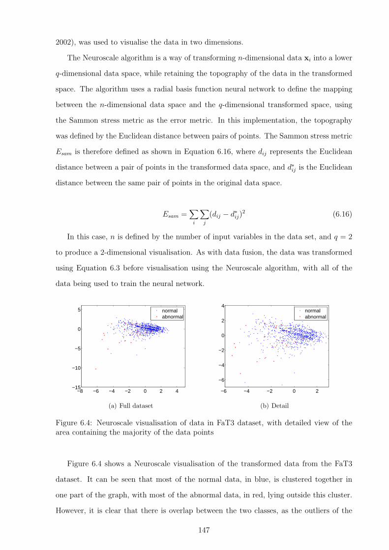
2002), was used to visualise the data in two dimensions.

The Neuroscale algorithm is a way of transforming n-dimensional data xi into a lower

q-dimensional data space, while retaining the topography of the data in the transformed

space. The algorithm uses a radial basis function neural network to define the mapping

between the n-dimensional data space and the q-dimensional transformed space, using

the Sammon stress metric as the error metric. In this implementation, the topography

was defined by the Euclidean distance between pairs of points. The Sammon stress metric

Esam is therefore defined as shown in Equation 6.16, where dij represents the Euclidean

distance between a pair of points in the transformed data space, and d∗ij is the Euclidean

distance between the same pair of points in the original data space.

Esam =∑

i

∑

j

(dij − d∗ij)2 (6.16)

In this case, n is defined by the number of input variables in the data set, and q = 2

to produce a 2-dimensional visualisation. As with data fusion, the data was transformed

using Equation 6.3 before visualisation using the Neuroscale algorithm, with all of the

data being used to train the neural network.

−8 −6 −4 −2 0 2 4−15

−10

−5

0

5

normalabnormal

(a) Full dataset

−6 −4 −2 0 2

−6

−4

−2

0

2

4

normalabnormal

(b) Detail

Figure 6.4: Neuroscale visualisation of data in FaT3 dataset, with detailed view of thearea containing the majority of the data points

Figure 6.4 shows a Neuroscale visualisation of the transformed data from the FaT3

dataset. It can be seen that most of the normal data, in blue, is clustered together in

one part of the graph, with most of the abnormal data, in red, lying outside this cluster.

However, it is clear that there is overlap between the two classes, as the outliers of the

147

normal data occur in similar areas to the abnormal data, and a few abnormal data points

lie in the area where most of the normal data is clustered.

−8 −6 −4 −2 0 2 4−10

−5

0

5

normalabnormal

Figure 6.5: Neuroscale visualisation of data in Walsgrave3 dataset

−4 −2 0 2 4 6 8−4

−2

0

2

4

6

8

normalabnormal

Figure 6.6: Neuroscale visualisation of data in Walsgrave4 dataset

Figures 6.5 and 6.6 show the equivalent visualisations for the Walsgrave3 and Wals-

grave4 datasets. These graphs show even more overlap between the normal and abnormal

data than for the FaT3 dataset. This could indicate that the classification errors in these

datasets may be worse than in the FaT3 dataset.

6.4 Comparison of data fusion methods

The five data fusion methods described in Section 6.1 were initially assessed using the

FaT3 dataset and the experimental method described above. The PAWS-3 score was also

148

calculated for the FaT3 dataset to be used as a comparator.

6.4.1 Linear regression

The graph in Figure 6.7(a) shows summary ROC curves for linear regression. These

represent the median, and 10th and 90th centiles of the ROC curves generated by the

jack-knifing procedure. The graph shows good performance when classifying the FaT3

dataset using linear regression, and also shows that the shape of the ROC curve did not

change greatly between tests.

0 0.2 0.4 0.6 0.8 10

0.2

0.4

0.6

0.8

1

Sen

sitiv

ity

1 − Specificity

median10% and 90% centiles

(a) ROC curve

−0.5 0 0.5 1 1.5 2 2.50

0.5

1

1.5

2

2.5

Output value

p(x)

normalabnormal

(b) Empirical probability density functions

Figure 6.7: Results of linear regression tests using FaT3 dataset

The area under each jack-knifed ROC curve was calculated, and summary statistics

were calculated from these values. The median AUC was 0.82, indicating acceptable

classification performance, with values of 0.79 and 0.83 for the 10th and 90th percentiles

respectively.

The sensitivity and specificity were calculated for each ROC curve at the point with

the minimum distance to the (0, 1) point. The median (10%–90%) sensitivity for linear

regression was 81.0% (75.6–84.4), and the specificity was 70.7% (66.7–74.8).

Figure 6.7(b) shows the empirical probability density functions of the output values

from the linear regression model. In the training dataset, normal data was coded as 0, and

abnormal data was coded as 1. As expected, there was significant overlap between the

two functions, showing that perfect separation of the two classes using linear regression

would not be possible.

149

6.4.2 Logistic regression

Figure 6.8(a) shows the summary ROC curves for logistic regression. These are similar

to those seen previously for linear regression, but a comparison shows that the curve for

logistic regression tends to lie closer to the (0, 1) point than the curve for linear regression,

indicating better separation of the two classes.

0 0.1 0.2 0.3 0.4 0.5 0.6 0.7 0.8 0.9 10

0.1

0.2

0.3

0.4

0.5

0.6

0.7

0.8

0.9

1

Sen

sitiv

ity

1 − Specificity

median10% and 90% centiles

(a) ROC curve

0 0.1 0.2 0.3 0.4 0.5 0.6 0.7 0.8 0.9 10

5

10

15

20

25

30

35

40

45

Output value

p(x)

normalabnormal

(b) Empirical probability density functions

Figure 6.8: Results of logistic regression tests using FaT3 dataset

There was also a considerable difference between the empirical probability density

functions produced by linear and logistic regression. As previously discussed, the output

of logistic regression is limited to the range (0, 1), and this can be seen in Figure 6.8(b).

This figure shows that the outputs from the normal data were very tightly clustered

around 0, as would be expected in a well-performing model. Ideally, the outputs from

the abnormal data would be clustered around 1 in a similar manner. Although this is not

the case, the tight clustering of the normal data allowed a threshold to be chosen that

produces good separation between the two classes.

The median (10%–90%) AUC for logistic regression was 0.83 (0.81–0.85), showing that

this technique classified this data marginally more accurately than linear regression. The

optimal sensitivity (closest to the (0, 1) point) was 75.8% (72.0–80.0), and the equivalent

specificity was 75.8% (71.7–79.8).

150

6.4.3 Gaussian mixture model classifiers

Twenty-four different Gaussian mixture model classifiers were investigated, using all pos-

sible combinations of kns and ks given in Equations 6.14 and 6.15. Figure 6.9 compares

the area under the ROC curve for all 24 combinations, showing the median, 10th and

90th centiles of AUC.

1 3 5 7 9 10 20 500.6

0.65

0.7

0.75

0.8

0.85

Number of normal kernels

Are

a un

der

RO

C c

urve

1 abnormal kernels3 abnormal kernels5 abnormal kernels

Figure 6.9: Area under ROC curve for GMM classifiers with various numbers of kernels

It is clear from Figure 6.9 that using one abnormal kernel produced the best AUC

results. There was also a general trend towards better performance with fewer kernels in

the GMM modelling the normal data, although this did not have such a large effect as

increasing the number of abnormal kernels.

To better understand these results, typical GMM classifiers were trained on the full

FaT3 dataset with 1, 3 and 5 normal and abnormal kernels. To visualise the shape of

these kernels, 2000 points were sampled from each GMM (i.e. normal and abnormal),

with the likelihood of sampling from each kernel equal to the prior for that kernel. These

samples were then transformed using the same Neuroscale model as was used to create

Figure 6.4. The resulting visualisations are shown in Figure 6.10.

From Figure 6.10, we can see that increasing the number of normal kernels between

one and five did not significantly change the distribution of the data, explaining why there

was little difference in the accuracy of the model. However, Figure 6.10 shows clearly that

increasing the number of kernels in the abnormal GMM caused considerable overfitting

to the data. It is likely that this was the cause of the decreased accuracy when more than

151

k(no

rmal

) =

1

Distribution of typical GMM classifier models

k(no

rmal

) =

3

k(abnormal) = 1

k(no

rmal

) =

5

k(abnormal) = 3 k(abnormal) = 5

Figure 6.10: Neuroscale visualisation of sampled points from typical Gaussian mixturemodels trained on the FaT3 dataset with 1, 3, and 5 normal and abnormal kernels. Pointssampled from GMMs trained on normal data are shown in blue, and points sampled fromGMMs trained on abnormal data are shown in red.

one kernel is used for the abnormal GMM.

The best performing GMM classifier, with one kernel for each class, had an AUC value

of 0.83 (0.81–0.85), with a sensitivity closest to the (0, 1) point of 79.0% (75.7–84.3), and

a specificity of 75.8% (70.7–79.8).

6.4.4 Gaussian mixture model novelty detectors

GMM novelty detectors were tested using all eight different values of kns given in Equation

6.14. Figure 6.11 compares the AUC values for the different options, showing the median,

10th, and 90th centiles.

Unlike the GMM classifiers, it would appear that a single kernel did not produce the

best results for the GMM novelty detectors. This observation underlines the differences in

operation between classifiers and novelty detectors. For a classifier, accuracy is dependent

on the boundary between the normal and abnormal models, and so a less detailed model

of the normal data may work well if there is a good model of the abnormal data. However,

in novelty detection, the boundary is defined purely by the model of the normal data,

152

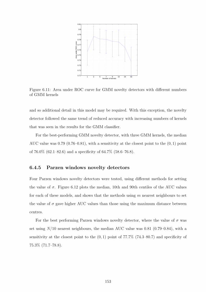
1 3 5 7 9 10 20 500.71

0.72

0.73

0.74

0.75

0.76

0.77

0.78

0.79

0.8

0.81

Number of kernelsA

rea

unde

r R

OC

cur

ve

Figure 6.11: Area under ROC curve for GMM novelty detectors with different numbersof GMM kernels

and so additional detail in this model may be required. With this exception, the novelty

detector followed the same trend of reduced accuracy with increasing numbers of kernels

that was seen in the results for the GMM classifier.

For the best-performing GMM novelty detector, with three GMM kernels, the median

AUC value was 0.79 (0.76–0.81), with a sensitivity at the closest point to the (0, 1) point

of 76.0% (62.1–82.6) and a specificity of 64.7% (58.6–76.8).

6.4.5 Parzen windows novelty detectors

Four Parzen windows novelty detectors were tested, using different methods for setting

the value of σ. Figure 6.12 plots the median, 10th and 90th centiles of the AUC values

for each of these models, and shows that the methods using m nearest neighbours to set

the value of σ gave higher AUC values than those using the maximum distance between

centres.

For the best performing Parzen windows novelty detector, where the value of σ was

set using N/10 nearest neighbours, the median AUC value was 0.81 (0.79–0.84), with a

sensitivity at the closest point to the (0, 1) point of 77.7% (74.3–80.7) and specificity of

75.3% (71.7–78.8).

153

10 nearest N/10 nearest sqrt(max distance) max distance0.68

0.7

0.72

0.74

0.76

0.78

0.8

0.82

0.84

0.86

Parzen sigma estimatorA

rea

unde

r R

OC

cur

ve

Figure 6.12: Area under ROC curve for Parzen windows novelty detectors using differentmethods for setting the value of σ

6.4.6 Comparison of different methods

The ten methods with the best classification results were compared to each other, and

also to the PAWS-3 reference classifier:

•linear regression

•logistic regression

•GMM classifiers with 1 abnormal kernel

– 1 normal kernel

– 3 normal kernels

– 5 normal kernels

•GMM novelty detectors

– 1 GMM kernel

– 3 GMM kernels

– 5 GMM kernels

•Parzen windows novelty detectors using m nearest neighbours to set σ

– m = 10

– m = N/10

Figure 6.13 shows the median, 10th and 90th centiles of the AUC values for each of

the ten methods. This shows that both logistic regression and the GMM classifier with a

154

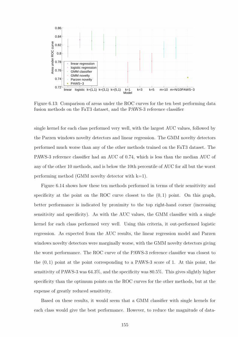
linear logistic k=(1,1) k=(3,1) k=(5,1) k=1 k=3 k=5 m=10 m=N/10PAWS−30.72

0.74

0.76

0.78

0.8

0.82

0.84

0.86

Model

Are

a un

der

RO

C c

urve

linear regressionlogistic regressionGMM classifierGMM noveltyParzen noveltyPAWS−3

Figure 6.13: Comparison of areas under the ROC curves for the ten best performing datafusion methods on the FaT3 dataset, and the PAWS-3 reference classifier

single kernel for each class performed very well, with the largest AUC values, followed by

the Parzen windows novelty detectors and linear regression. The GMM novelty detectors

performed much worse than any of the other methods trained on the FaT3 dataset. The

PAWS-3 reference classifier had an AUC of 0.74, which is less than the median AUC of

any of the other 10 methods, and is below the 10th percentile of AUC for all but the worst

performing method (GMM novelty detector with k=1).

Figure 6.14 shows how these ten methods performed in terms of their sensitivity and

specificity at the point on the ROC curve closest to the (0, 1) point. On this graph,

better performance is indicated by proximity to the top right-hand corner (increasing

sensitivity and specificity). As with the AUC values, the GMM classifier with a single

kernel for each class performed very well. Using this criteria, it out-performed logistic

regression. As expected from the AUC results, the linear regression model and Parzen

windows novelty detectors were marginally worse, with the GMM novelty detectors giving

the worst performance. The ROC curve of the PAWS-3 reference classifier was closest to

the (0, 1) point at the point corresponding to a PAWS-3 score of 1. At this point, the

sensitivity of PAWS-3 was 64.3%, and the specificity was 80.5%. This gives slightly higher

specificity than the optimum points on the ROC curves for the other methods, but at the

expense of greatly reduced sensitivity.

Based on these results, it would seem that a GMM classifier with single kernels for

each class would give the best performance. However, to reduce the magnitude of data-

155

0.55 0.6 0.65 0.7 0.75 0.8 0.85 0.90.55

0.6

0.65

0.7

0.75

0.8

0.85

Sensitivity

Spe

cific

ity

linear regressionlogistic regressionGMM classifier k=(1,1)GMM classifier k=(3,1)GMM classifier k=(5,1)GMM novelty k=1GMM novelty k=3GMM novelty k=5Parzen novelty 10 nearestParzen novelty N/10 nearestPAWS−3

Figure 6.14: Comparison of sensitivity and specificity at the point on the ROC curveclosest to the (0, 1) point for the ten best performing data fusion methods, and the PAWS-3 reference classifier. Markers are positioned at the median point, with the dotted linesshowing the range covered by the 10th–90th centiles.

dependent effects, the performance of this data fusion method was also assessed using

an independent dataset (as in Section 6.5), with logistic regression, linear regression, and

Parzen windows novelty detection (using both m = 10 and m = N/10 nearest neighbours

to set the value of σ) also being assessed on the independent dataset.

6.4.7 Varying the number of data points in the testing set

All of the results described so far were obtained using testing sets consisting of 3 normal

and 3 abnormal data points in each jack-knife iteration. It was hypothesised that a small

number of test points should be used in each iteration to ensure that there would be a

sufficient number of abnormal data points in the training set to allow adequate training

of the regression and GMM classifier models. The FaT3 dataset contains 845 normal

data points, but only 28 abnormal data points. The maximum number of test points was

therefore limited by the number of abnormal data points, and so the amount of normal

data in the training set would not be greatly affected by the size of the test set. It was

therefore hypothesised that the results obtained with the novelty detectors, which were

156

trained only on the normal data, would not be significantly affected by changing the size

of the test set.

To assess the effect of changing the size of the test set, the ten best performing models

were re-assessed using test sets containing 1, 14, and 20 of each type of data point. The

results of these experiments on the area under the ROC curve are shown in Figure 6.15.

linear logistic k=(1,1) k=(3,1) k=(5,1) k=1 k=3 k=5 m=10 m=N/100.7

0.72

0.74

0.76

0.78

0.8

0.82

0.84

0.86

0.88

Model

Are

a un

der

RO

C c

urve

n=1n=3n=14n=20

Figure 6.15: Comparison of area under the ROC curve for the ten best performing modelswhen tested with test sets of different sizes

Figure 6.15 confirms the hypothesis that changing the size of the test set had little

effect on the performance of the novelty detectors, with the exception that the larger test

sets resulted in the 10th and 90th centiles being closer to the median. This was expected,

as the ROC curves from larger test sets would be smoother, and hence give more accurate

estimates of the true area under the curve.

As n increased, the performance of the regression models and GMM classifiers tended

to decrease. This was also as predicted, as there were fewer abnormal data points available

in any given iteration to train the models. This phenomenon was particularly noticeable

for n = 20, when only 8 abnormal data points were available for training the data fusion

model. However, the effect was not noticeable at n = 3, and so it appears that the original

choice of the number of points to retain in the testing set was valid.

6.5 Comparison of best performing methods on in-

dependent dataset

Ideally, the Walsgrave3 dataset would have been used as an independent test set for data

fusion methods which had been trained using the FaT3 dataset. However, the difference in

157

the populations and classifications for the two datasets made this an impractical proposi-

tion. The FaT3 dataset consists of children attending primary care, with the classification

of severity based on admission to hospital, which was only observed in 3% of the subjects.

In contrast, the Walsgrave3 dataset consists entirely of children admitted to a hospital

ward, of whom 16% are classified as having a potentially life-threatening infection. All

of the children in the Walsgrave3 dataset would therefore be classified in the abnormal

class for the FaT study, and their vital signs are likely to lie in a much larger area of the

data space than the small number of abnormal children in the FaT3 dataset. Therefore,

a classification method developed using the FaT3 dataset would not be expected to show

good performance when tested on the Walsgrave3 dataset. Tests using the Walsgrave3

dataset were therefore performed in the same manner as those using the FaT3 dataset,

with jack-knifing providing independent training and test datasets, and the results being

combined to calculate ROC curves.

The Walsgrave3 dataset is a more challenging test for a data fusion model than the

FaT3 dataset for a number of reasons. The dataset is smaller, meaning that there are

fewer data points available for training the model, and the initial visualisation using the

Neuroscale algorithm in Figure 6.5 showed that there was a greater overlap between the

two classes than is the case for the FaT3 data. A worse classification performance was

therefore expected on this dataset than on the FaT3 dataset. However, it was still possible

to use it to compare the performance of different data fusion models.

The best performing five models identified in the previous section were tested in the

same manner as previously, but using the Walsgrave3 dataset to provide the training

and test sets. The PAWS-3 reference classifier was also tested to provide an independent

comparator. The models investigated were: linear regression, logistic regression, GMM

classifier using single kernels for each class, and Parzen windows novelty detection using

both m = 10 and m = N/10 nearest neighbours to set the value of σ.

Figure 6.16 compares the empirical probability density functions produced by the

output of the linear regression models trained on the FaT3 and Walsgrave3 datasets.

This shows that there was much greater overlap between the outputs from the two classes

for the Walsgrave3 dataset, indicating that separation was more difficult. This was also

158

−0.5 0 0.5 1 1.5 2 2.50

0.5

1

1.5

2

2.5

Output value

p(x)

normalabnormal

(a) FaT3

0 0.5 1 1.50

1

2

3

4

5

Output value

p(x)

normalabnormal

(b) Walsgrave3

Figure 6.16: Empirical probability density functions for output of linear regression modelon data from FaT3 and Walsgrave3 datasets

confirmed by comparing the performance of the models, summarised in Table 6.3, with

the equivalent values for the models trained on the FaT3 dataset. The models trained

on the Walsgrave3 dataset showed smaller areas under the ROC curve, as well as lower

sensitivities and specificities at the point on the curve closest to the (0, 1) point.

Model AUC Sensitivity (%) Specificity (%)Linear Regression 0.659 (0.64–0.68) 64.3 (61.2–68.9) 60.6 (56.6–64.7)Logistic Regression 0.667 (0.64–0.69) 63.7 (59.5–68.1) 60.6 (55.6–65.7)GMM classifier (1,1) 0.669 (0.64–0.70) 61.7 (57.7–64.8) 65.7 (61.6–69.7)Parzen windows (m = 10) 0.662 (0.63–0.69) 61.4 (57.2–66.5) 65.2 (60.6–69.7)Parzen windows (m = N/10) 0.662 (0.63–0.68) 61.7 (57.5–65.3) 66.7 (62.2–70.7)PAWS-3 0.623 66.4 51.6

Table 6.3: Median (10–90%) area under ROC curve, sensitivity and specificity at point oncurve closest to the (0, 1) point for models trained and tested on the Walsgrave3 dataset

The values in Table 6.3 and the graphs in Figure 6.17 show that there is not much

difference in classification performance between the five data fusion methods trained and

tested on the Walsgrave3 dataset. In terms of the area under the ROC curve, the GMM

classifier again appeared to outperform the other methods, although by a very small

margin, with the linear regression model performing least well. However, the Parzen

windows model with σ set using m = N/10 nearest neighbours appeared to perform

slightly better in terms of sensitivity and specificity at the point closest to the (0, 1)

point. The PAWS-3 again performs worse than the more complex methods, although the

difference is not as great as was seen with the FaT3 dataset.

159

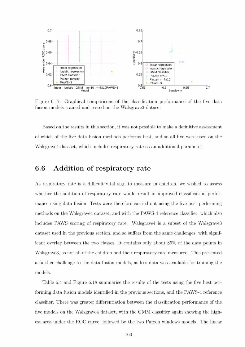
linear logistic GMM m=10 m=N/10PAWS−30.6

0.62

0.64

0.66

0.68

0.7

Model

Are

a un

der

RO

C c

urve

linear regressionlogistic regressionGMM classifierParzen noveltyPAWS−3

0.55 0.6 0.65 0.70.5

0.55

0.6

0.65

0.7

0.75

Sensitivity

Spe

cific

ity

linear regressionlogistic regressionGMM classifierParzen m=10Parzen m=N/10PAWS−3

Figure 6.17: Graphical comparisons of the classification performance of the five datafusion models trained and tested on the Walsgrave3 dataset

Based on the results in this section, it was not possible to make a definitive assessment

of which of the five data fusion methods performs best, and so all five were used on the

Walsgrave4 dataset, which includes respiratory rate as an additional parameter.

6.6 Addition of respiratory rate

As respiratory rate is a difficult vital sign to measure in children, we wished to assess

whether the addition of respiratory rate would result in improved classification perfor-

mance using data fusion. Tests were therefore carried out using the five best performing

methods on the Walsgrave4 dataset, and with the PAWS-4 reference classifier, which also

includes PAWS scoring of respiratory rate. Walsgrave4 is a subset of the Walsgrave3

dataset used in the previous section, and so suffers from the same challenges, with signif-

icant overlap between the two classes. It contains only about 85% of the data points in

Walsgrave3, as not all of the children had their respiratory rate measured. This presented

a further challenge to the data fusion models, as less data was available for training the

models.

Table 6.4 and Figure 6.18 summarise the results of the tests using the five best per-

forming data fusion models identified in the previous sections, and the PAWS-4 reference

classifier. There was greater differentiation between the classification performance of the

five models on the Walsgrave4 dataset, with the GMM classifier again showing the high-

est area under the ROC curve, followed by the two Parzen windows models. The linear

160

Model AUC Sensitivity (%) Specificity (%)Linear Regression 0.665 (0.64–0.69) 63.4 (58.0–68.4) 60.6 (57.1–67.7)Logistic Regression 0.668 (0.65–0.69) 62.0 (57.0–66.5) 63.6 (57.6–67.7)GMM classifier (1,1) 0.685 (0.66–0.72) 64.6 (60.6–68.2) 65.7 (61.6–69.7)Parzen windows (m = 10) 0.681 (0.65–0.71) 64.7 (61.1–68.7) 67.7 (64.7–71.7)Parzen windows (m = N/10) 0.673 (0.65–0.70) 61.8 (64.9–69.9) 71.7 (65.2–76.8)PAWS-4 0.641 73.1 49.5

Table 6.4: Median (10–90%) area under ROC curve, sensitivity and specificity at point oncurve closest to the (0, 1) point for models trained and tested on the Walsgrave4 dataset

regression model again gave the worst classification performance of the five in terms of

the area under the ROC curve, although it still performed considerably better than the

PAWS-4 reference classifier. If the optimal sensitivity and specificity were required, the

Parzen windows models and the GMM classifier gave the best performance. The optimal

sensitivity and specificity for the PAWS-4 classifier was obtained at a PAWS-4 score of 2,

and gave considerably higher sensitivity than was seen at the optimal points for the other

methods. However, this was at the expense of greatly decreased specificity, at less than

50%.

linear logistic GMM m=10 m=N/10PAWS−40.6

0.62

0.64

0.66

0.68

0.7

0.72

Model

Are

a un

der

RO

C c

urve

linear regressionlogistic regressionGMMParzen windowsPAWS−4

0.45 0.5 0.55 0.6 0.65 0.70.55

0.6

0.65

0.7

0.75

0.8

Sensitivity

Spe

cific

ity

linear regressionlogistic regressionGMMParzen m=10Parzen m=N/10PAWS−4

Figure 6.18: Graphical comparisons of the performance of the five data fusion modelstested on the Walsgrave4 dataset, and the PAWS-4 reference classifier

When the values in Table 6.4 are compared to the results in Table 6.3, which shows

the equivalent results for the Walsgrave3 dataset, it can be seen that the addition of

respiratory rate did confer a consistent benefit in terms of the area under the ROC curve,

and also improved the sensitivity and specificity at the point closest to the (0, 1) point for

the GMM classifier and Parzen windows models. However, this increase was not very large,

161

Dataset HR Temperature SpO2 BRFaT3 37.8% 32.0% 30.3% –Walsgrave3 31.8% 40.0% 28.2% –Walsgrave4 26.1% 33.3% 21.9% 18.7%

Table 6.5: Percentages showing which vital sign is most abnormal in non-serious cases

Dataset HR Temperature SpO2 BRFaT3 10.7% 35.7% 53.6% –Walsgrave3 25.0% 30.8% 44.2% –Walsgrave4 19.4% 30.1% 35.5% 15.1%

Table 6.6: Percentages showing which vital sign is most abnormal in serious cases

and so it might be supposed that much of the information contained in the respiratory

rate was correlated with one or more of the other three variables (heart rate, temperature,

or SpO2). This agrees with an understanding of the physiological interactions between

respiratory rate and other vital signs. A high respiratory rate may indicate increased

respiratory effort, which would tend to result in a high heart rate, and is also indicative of

breathing difficulties, which may results in lowered levels of SpO2. In addition, fever (high

temperature) can lead to increased metabolic demands, resulting in increases in both the

respiratory rate and heart rate (Davies and Maconochie, 2009).

6.7 Predictivity of individual vital signs

In the context of data fusion, an investigation of the ‘most abnormal’ vital sign for a

given patient may indicate how the addition or removal of this vital sign would affect the

performance of a data fusion model. This was carried out by determining which of the

transformed vital signs had the largest absolute value, as this indicates which vital sign

is furthest from the mean, and thus most abnormal.

Table 6.5 and 6.6 show how frequently each vital sign is the most abnormal in non-

serious (normal) and serious (abnormal) cases respectively. These figures are shown graph-

ically in the form of pie charts for each dataset in Figures 6.19–6.21.

As would be expected, the distribution of the most abnormal data was approximately

equally spread among the vital signs for the non-serious cases in all three data sets.

However, this was not the case when the serious cases were investigated. In particular,

the SpO2 value was most abnormal in many serious cases. The temperature also appeared

162

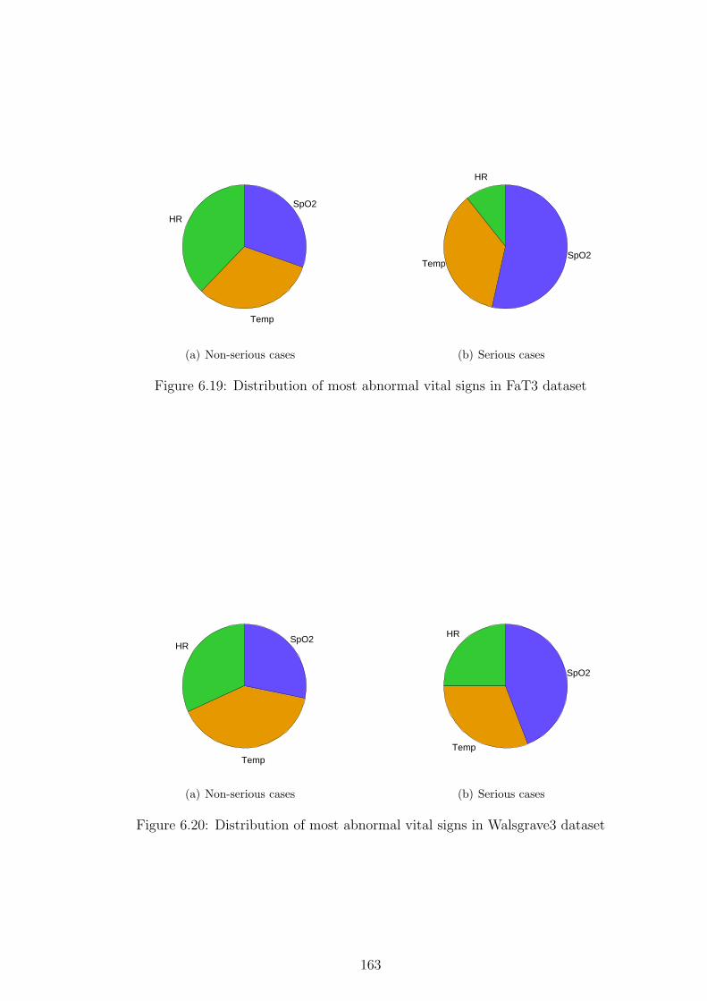
HR

Temp

SpO2

(a) Non-serious cases

HR

TempSpO2

(b) Serious cases

Figure 6.19: Distribution of most abnormal vital signs in FaT3 dataset

HR

Temp

SpO2

(a) Non-serious cases

HR

Temp

SpO2

(b) Serious cases

Figure 6.20: Distribution of most abnormal vital signs in Walsgrave3 dataset

163

to be a major factor in a number of cases, with fewer cases having extremely abnormal

heart rate or respiratory rate.

HR

RRTemp

SpO2

(a) Non-serious cases

HR

RR

Temp

SpO2

(b) Serious cases

Figure 6.21: Distribution of most abnormal vital signs in Walsgrave4 dataset

These findings show that SpO2 and temperature are likely to be particularly important

variables to include in a data fusion model, as they tended to become the most abnormal

in serious illness. However, it was still the case that many sick children also had highly

abnormal heart rates or respiratory rates, and hence these variables do need to be included

in data fusion models.

6.8 Summary

In this chapter, a number of different data fusion methods have been compared using

the FaT and Walsgrave vital sign datasets for training and testing of the models. Across

all three datasets tested, the Gaussian mixture model classifier with one kernel for both

normal and abnormal classes achieved the largest area under the ROC curve. However, a

number of other methods also performed similarly well, and should not be discounted at

this stage. These included Parzen windows novelty detectors trained using the m nearest

neighbours method, where m = 10 or m = N/10, and logistic regression. Since logistic

regression outperformed linear regression in all of the tests, it is suggested that logistic

regression be the preferred regression method for data fusion of vital signs in paediatric

triage.

Two reference classifiers were tested to assess the ability of data fusion methods to

164

outperform existing clinical scoring systems. These classifiers were developed by extract-

ing scorings for the relevant vital signs from the PAWS scoring system. It was seen that

these scores consistently underperformed the data fusion methods, with lower areas under

the ROC curve, and less good performance in terms of sensitivity and specificity.

The area under the ROC curve obtained for the best performing method in the FaT3

dataset was 0.83. This is comparable to the areas under the ROC curve reported for

PAWS (0.86), Toronto PEWS (0.83–0.90), and Cardiff and Vale PEWS (0.86) (Egdell

et al., 2008; Duncan et al., 2006; Edwards et al., 2009). It should be noted that these

systems were designed and tested in secondary care, with very different outcomes to those

in the FaT3 dataset, but confirms that this level of accuracy is likely to be sufficient for

clinical use, despite the small number of vital signs used.

This high level of accuracy was not replicated in either of the Walsgrave datasets,

where the achieved accuracy may not be sufficient for clinical use. This is likely to be due

to the makeup of this dataset, and the choice of outcome measure, which resulted in a

large degree of overlap between vital signs in the two groups of children. It is possible that

the results from the Walsgrave and FaT databases overestimate the performance of these

methods, as the vital signs were measured in a standardised way, with heart rate and

SpO2 measured using a pulse oximeter, temperature using a recently calibrated electronic

axillary thermometer, and only respiratory rate measured using clinical counting, which

is most likely to show large degrees of measurement error. In a typical clinical situation,

it is likely that larger error rates would be seen, due to a lack of calibration of electronic

devices, or human error in the case of clinical counting.

With the limited datasets available for the work described in this thesis, it was not

possible to determine a clear advantage to using any single data fusion method, and it

may be that some methods are more suited to certain data sources than others. It would

also be valuable to test the effect of including additional variables such as respiratory

rate with a larger dataset, as this did not show a significant advantage for the small

Walsgrave4 dataset. A larger dataset would also allow data to be trained and tested on

independent subsets, without the need for the jack-knifing technique used in this thesis.

This could also be achieved by the use of multiple smaller data sets with consistent or

165

comparable populations and outcome measures, such that a method trained on one set

could be realistically applied to another. Unfortunately, this was not possible with the

FaT and Walsgrave datasets due to the large differences in the populations, with the

inclusion criteria for the Walsgrave study corresponding to a higher level of acuity than

the definition of a serious outcome in the FaT study.

Predictions made using one-off measurements of vital signs are likely to suffer from

a number of confounding factors. Respiratory rate is under conscious control, and so

the value measured may be changed simply by the fact that a patient is aware that their

breathing is being monitored. As previously discussed, psychological stress may also affect

the measured values, with respiratory rate and heart rate being particularly likely to be

affected. Unobtrusive automated monitoring may mitigate these effects to some extent,

but the act of attaching monitoring equipment, or merely being in a clinical environment,

may be sufficiently stressful to alter vital signs measured in a child. Where it is possible to

monitor vital signs over a longer period, trend information is likely to be more informative

that a “snapshot” measurement, as acclimatisation to both monitoring and the clinical

environment may reduce the effects of stress, and any changes relevant to the clinical

picture will become apparent. However, the typical length of primary care consultations

is unlikely to make sure measurements a practical option.

Perfect prediction using only vital signs is unlikely to be possible. Even if a child has

normal or near-normal vital signs, they may have other signs or symptoms, such as severe

pain, rashes, or a concerning clinical history, which should inform clinical decision-making

(Bradman and Maconochie, 2008; Sandell et al., 2009). Thus the output of a data fusion

system as developed in this chapter can only be an aid to identification of serious illness,

rather than replacing a clinician’s detailed assessment.

166

Chapter 7

Conclusions

The work reported in this thesis has shown that it is possible to measure a variety of

vital signs, including respiratory rate, in children, using two simple non-invasive probes:

a pulse oximeter finger probe and a thermometer. It has also been shown that fusion of

these vital signs can be used as a tool to identify children with serious illness, and that

this technique may be viable in clinical practice.

The major areas of research explored in this thesis include:

• A meta-analysis of clinical measurements of heart rate and respiratory rate in normal

children (Chapter 2).

• Review of existing methods for estimating the respiratory rate from the photo-

plethysmogram in adult populations, and development of a novel method based on

autoregressive modelling (Chapters 3 and 4).

• Development and validation of an autoregressive modelling method for the estima-

tion of paediatric respiratory rates (Chapter 5).

• Assessment of the diagnostic accuracy of data fusion methods applied to paediatric

vital sign data acquired from patients in primary and emergency care (Chapter 6).

7.1 Overview

In Chapter 2, it was shown that existing reference ranges for heart rate and respiratory

rate are inconsistent, and may be inaccurate. A systematic meta-analysis of the clinical

167

literature was carried out, resulting in the production of non-parametric fitted curves for

the mean and standard deviation of normal heart rates and respiratory rates for children

aged between birth and 18 years of age. These curves were used to perform age correction

of heart rate and respiratory rate for children measured in clinical settings, and were

shown to remove much of the age dependence in this data.

This meta-analysis provides an evidence base for the variation of two important clinical

parameters during childhood and adolescence. The information can be used to correct

for the effect of age when performing data fusion on vital sign data, and may also assist

clinicians in their assessment of the degree of abnormality present in these vital signs

when monitoring unwell children.

Chapters 3 and 4 used pulse oximetry data from adult subjects to assess the accuracy

of a number of methods for estimating the respiratory rate from the photoplethysmogram

(PPG). Both amplitude and frequency modulation of the PPG were investigated, on data

acquired from both healthy and unwell subjects. It was shown that a novel method using

autoregressive modelling performed best in both AM and FM contexts, and that Kalman

filtering of the respiratory rates estimated using this technique was able to reduce the

influence of erroneous estimates of respiratory rate.

In Chapter 5, the method developed in Chapter 4 was adjusted to allow detection

of the higher respiratory rates observed in children, and was tested on two sets of data

collected for this thesis. It was found that estimation of respiratory rate from the PPG is

more challenging in the paediatric context, with higher levels of error observed, although

good estimates were obtained in over half of the subjects, who were monitored in a clinical

primary care environment.

It was hypothesised that much of the difficulty in the estimation of respiratory rates

in children was due to poor PPG signal quality. Sensor issues such as movement artefact

and poor probe placement were likely to be responsible for much of this, but physiological

factors also played a part. High respiratory rates, irregular breathing, and the use of

accessory muscles could all decrease the ability of the AR model to accurately estimate

the respiratory rate. In addition, serious illness and certain medications may reduce the

strength of respiratory sinus arrhythmia, the source of the frequency-modulated respira-

168

tory information in the PPG waveform.

Chapter 6 showed that a variety of data fusion methods can be used to predict the

severity of illness in children attending primary or emergency care settings, and that these

outperform equivalent classifiers derived from an existing paediatric early warning system.

The Gaussian mixture model classifier using a single kernel model for both the normal and

abnormal classes was shown to produce the best results for all three datasets under test.

However, the performance of this method was only marginally better than that observed

using Parzen windows novelty detectors or logistic regression, indicating that the optimal

choice from these methods may be data dependent.

Novelty detection using Gaussian mixture models with small numbers of kernels per-

formed very poorly, and is unlikely to be of use for data fusion of paediatric vital signs.

The linear regression method is also unlikely to be of any benefit, as it was consistently

outperformed by logistic regression.

It was found that sensitivities and specificities of 65–80% were achievable using a

combination of 3 or 4 vital signs. The achievable accuracy was dependent on the source

of the data, with a primary care dataset proving to produce higher classification accuracies

than one collected in emergency care. This may be due to a number of factors such as

the inclusion criteria for each study, the chosen outcome, and the size of the population

studied.

7.2 Further work

7.2.1 Validation of meta-analysis results

The fitted curves for heart rate and respiratory rate presented in Chapter 2 have been

partially validated using the FaT and Walsgrave datasets. A further study to verify the

results of the meta-analysis using large numbers of measurements would be beneficial in

assessing the clinical utility of this new evidence base.

Data from normal, healthy children should be used to confirm the fit of the curves, and

could also be used to further investigate factors such as the accuracy of manual palpation

of paediatric heart rates, which were shown to result in lower measured values in the

169

meta-analysis. Data from children with a variety of illnesses and injuries should also be

assessed against the curves to determine the point at which abnormalities in heart rate

or respiratory rate become clinically significant. These datasets could be obtained by

carrying out a study to measure heart rate and respiratory rate in a large cohort of both

healthy and unwell children. However, it is likely that such data may have already been

collected as part of existing trials or studies that were not included in the meta-analysis,

and this may be a more practical method of efficiently obtaining large amounts of test

data.

Further sub-group analysis could also be carried out on the data used to create the

fitted curves. For example, it would be interesting to assess whether some studies report

consistently low or high values of heart rate or respiratory rate, and to investigate possible

reasons for this. It may also be possible to assess the effect of other parameters, such as

gender, ethnicity, and the age of the study1 (i.e. how long ago it was carried out) to see

if these have an effect on the measured values.

7.2.2 Improvement of respiratory rate estimation using the PPG

The results from Chapter 5 show that the AR model often contained a pole close to

the true respiratory rate, but that this pole was not always identified as the breathing

pole due to its low magnitude. Many of the PPG waveforms were observed to have poor

signal quality, which was likely to affect the ability of the algorithm to identify the correct

respiratory rate.

Some of the causes of poor quality PPG may be able to be minimised by improving

the placement of the PPG probe. In the OXEMS and Oxford School studies, many of

the children were monitored using clip-style probes, which are likely to be particularly

vulnerable to motion artefact and poor probe placement. An alternative would be to use

wrap-around probes with adhesive fixings, which should reduce artefacts due to movement

of the probe relative to the finger, as the probes are more securely attached.

Further pre-processing of the raw PPG signal may allow for better identification and

1The age of the study may have an effect on the measured heart rates and respiratory rates due toadvances in measurement techniques, and changes in the general health, and average height and weightof the children being studied.

170

removal of noise due to motion artefact or baseline wander. When using the PPCA-

derived novelty scores to remove sections of poor-quality PPG waveform, no effort was

made to replace the removed sections with padding, or smooth any discontinuities. Adding

padding could improve the estimation of the respiratory rate, as removal of a section of the

waveform could result in the extracted respiratory waveform having an artefactually high

frequency. In addition, discontinuities in the waveform may interfere with the detection

of salient points, or introduce high-frequency components into the frequency spectrum of

the waveform.

Only one algorithm for signal quality quantification was investigated in any depth in

this thesis. It would be beneficial to investigate the ability of other algorithms, and also

to consider the application of multiple signal quality indices, which could potentially be

combined to obtain a more accurate estimation of signal quality, or to identify periods of

data where one method of respiratory rate extraction (e.g. AM or FM) would be likely

to perform better than another.

Further improvements to the pole choice algorithm could include the development of

a Bayesian method, based on prior knowledge of the distribution of the likely respiratory

rates, given the child’s age and the known distribution of normal respiratory rates at that

age. This distribution could then be updated based on the location and magnitude of

poles in the AR models from both AM and FM analysis, the signal quality of the PPG

waveform, and the posterior distribution of likely respiratory rates from previous time

windows for that subject. The estimated respiratory rate could then be reported in terms

of a most likely value, and the level of confidence in that value.

The AM and FM methods of extracting respiratory rate from the PPG rely on signals

created by different physiological processes (pressure change in the thorax, and nervous

control of the heart rate). It might therefore be expected that the failure modes of these

two methods may not be completely correlated. Indeed, it was observed that only one

of the AR methods (AM or FM) produced an accurate estimation of the true respiratory

rate in a number of cases. However, initial attempts to fuse the results from the two

sources using a multi-dimensional Kalman filter did not produce much improvement in

the estimated respiratory rates, and so were not presented. This was also the case where

171

signal quality estimations were used to estimate the noise covariance as described in

Section 5.4.2. Although higher correlation would be expected for two estimates derived

from the same source that those from different physiological signals, fusion techniques

such as those described in Clifford et al. (2009), Nemati et al. (2010) and Kuan (2010)

may be worth further investigation. In cases where the AM and FM methods do not

agree on an estimated respiratory rate, it may be possible to investigate ways to identify

which method is more reliable in a given situation. A signal quality index based on the

pre-processed waveform rather than the original signal, as used in Nemati et al. (2010)

and Kuan (2010) is likely to be particularly useful in this situation.

7.2.3 Data fusion of vital signs

Further work is required to build on the initial data fusion investigations reported in this

thesis. These should include larger populations of children, with consistent outcomes in

both training and test datasets, to remove the need to carry out jack-knifing in order to

obtain sufficient points to construct an ROC curve. Since it is unlikely that a dataset

containing complete sets of vital signs for every child could be obtained, different methods

for imputing missing data could be investigated, and their effect on the resulting data

fusion models assessed.

The results of this work should lead to the development of a data fusion model that

can be applied in clinical practice. This should then be assessed in a clinical setting to

determine whether incorporating data fusion of vital signs into the clinical workflow has

an effect on the outcome of monitored children.

7.3 Proposed follow-up study

Ethics approval and funding have been obtained for a further research study based on the

work reported in this thesis. This study will be carried out in the Paediatric Emergency

Department (ED) at the John Radcliffe Hospital in Oxford. Children between 1 month

and 12 years of age who attend the ED with acute medical illness will be eligible for

inclusion. Those who are very unwell and require immediate medical intervention, or who

are attending for treatment of a traumatic injury will be excluded.

172

Data collection for this study will be carried out as a part of the normal triage process

in the Paediatric ED. The equipment to be used is similar to that used in the OXEMS

study described in Chapter 5, with the exception that automated monitoring of tem-

perature will not be carried out. To reduce the influence of motion artefact in younger

children, adhesive finger probes will be used to collect pulse oximetry data from children

under the age of two years. The automated monitoring will be used to assess the child’s

heart rate and SpO2, with other observations being carried out by the triage nurse accord-

ing to normal clinical practice. Since the oximeter to be used is identical to that used in

the OXEMS study, it is unlikely that useful measures of perfusion index will be obtained

from this study. However, capillary refill time is part of the usual set of observations

carried out in the triage process, and so this will be captured from the nursing records.

As it was hypothesised that much of the poor signal quality in the paediatric data sets

investigated in Chapter 5 was due to motion artefact, the triage nurse will also record

the child’s compliance on a four-point scale. The scale to be used was designed in con-

junction with ED nurses, and categorises the child into one of the following categories:

”Compliant”, ”Intermittent movement”, ”Frequent movement”, or ”Non-compliant”. Al-

though existing sedation-agitation scores, such as the Riker score (Riker et al., 1999)

exist, these were not felt to be appropriate here, as some children may exhibit frequent

movement during monitoring without any alteration in neurological status. Although a

subjective scale such as this is likely to result in both inter- and intra-observer variability,

it is believed that the simplicity of the score will reduce the impact of this, and that the

data obtained will be sufficient to enable the identification of children with and without

significant motion artefact on the PPG waveform.

Consent for research use of the data will typically be obtained after the monitoring

has been carried out, as the monitoring will form part of standard care in the ED. The

study intends to recruit a minimum of 400 children, with at least 100 children in each of

four age groups (0–1 years, 1–2 years, 2–5 years, and 5–12 years), and is expected to start

in January 2011.

Where consent is given, the child’s demographic data (age and gender), and the obser-

vations carried out at triage (temperature, respiratory rate, blood pressure, capillary refill

173

time, and GCS score) will be recorded from the patient’s notes. Where appropriate, any

respiratory distress or use of supplemental oxygen will also be recorded. This data would

enable better comparison of data fusion results with existing PEWS scoring systems. The

date and time of the child’s arrival at and departure from the ED will also be recorded,

so that the length of stay in the ED can be calculated.

Further outcome measures will also be recorded from the child’s notes and the hospital

computer system. These include any interventions carried out in the ED (e.g. blood tests,

imaging, or IV therapy), the discharge diagnosis, and details of any admission to hospital.

This study aims to assess the feasibility and reliability of the technology in a clinical

setting, including the time taken to obtain data, and how well the monitoring is tolerated

by unwell children. The PPG waveforms recorded from the children will be analysed to

validate the algorithms described in Chapter 5, with a manual measure of the respiratory

rate being used as the reference standard. In addition, the size of the study and the variety

of outcome measures will allow the vital sign data to be used to assess the performance

of data fusion methods as described in Chapter 6.

174

Bibliography

Abdurrahman L., Hoit B.D., Banerjee A., Khoury P.R., and Meyer R.A. Pulmonary

venous flow doppler velocities in children. J. Am. Soc. Echocardiogr., 11(2):132–7,

1998.

Adams F.H., Emmanouilides G.C., and Riemenscheider T.A., editors. Moss’ Heart Dis-

ease in Infants, Children and Adolescents. Williams and Wilkins, Baltimore, 4th edition,

1989.

Addison P. and Watson J. Secondary wavelet feature decoupling (SWFD) and its use

in detecting patient respiration from the photoplethysmogram. In: Conf. Proc. IEEE

Eng. Med. Biol. Soc, pages 2602–5. 2003.

Addison P.S. and Watson J.N. Secondary transform decoupling of shifted nonstationary

signal modulation components: application to photoplethysmography. Int. J. Wavelets

Multiresolut. Inf. Process., 2(1):43–57, 2004.

Advanced Life Support Group. Advanced Paediatric Life Support: The Practical Ap-

proach. WileyBlackwell, London, 4th edition edition, 2004.

Advanced Life Support Group. Pre Hospital Paediatric Life Support: The Practical Ap-

proach. WileyBlackwell, Oxford, 2nd edition edition, 2005.

Allen J. Photoplethysmography and its application in clinical physiological measurement.

Physiol. Meas., 28(3):R1–39, 2007.

Alpay F., Celiker A., Lenk M.K., Ozcan O., Tanindi S., and Isik E. Ambulatory electro-

cardiographic monitoring in healthy newborn infants. Turk. J. Pediatr., 35(3):163–70,

1993.

175

American College of Surgeons. ATLS: Advanced Trauma Life Support for Doctors. Amer-

ican College of Surgeons, Chicago, 7th edition edition, 2004.

American Heart Association. Pediatric Advanced Life Support Provider Manual. American

Heart Association, Dallas, 2006.

Anderson S.T., Downs W.G., Lander P., Mirvis D.M., Rizo-Patron C., Burr R.L., Ja-

cobson C., Massumi G.A., and Perry J.C. Advanced Electrocardiography. Biophysical

Measurement series. Spacelabs Medical, Redmond, Washington, 1995.

Andrasyova D. and Kellerova E. Blood pressure and heart rate response to head-up

position in full-term newborns. Early Hum. Dev., 44(3):169–78, 1996.

Antila K.J., Valimaki I.A., Makela M., Tuominen J., Wilson A.J., and Southall D.P. Heart

rate variability in infants subsequently suffering sudden infant death syndrome (SIDS).

Early Hum. Dev., 22(2):57–72, 1990.

Armon K., Stephenson T., Gabriel V., MacFaul R., Eccleston P., Werneke U., and Smith

S. Determining the common medical presenting problems to an accident and emergency

department. Arch. Dis. Child., 84(5):390–2, 2001.

Ashton R. and Connolly K. The relation of respiration rate and heart rate to sleep states

in the human newborn. Dev. Med. Child Neurol., 13(2):180–7, 1971.

Balasubramanian S., Suresh N., Ravichandran C., and Dinesh Chand G. Reference values

for oxygen saturation by pulse oximetry in healthy children at sea level in Chennai. Ann.

Trop. Paediatr., 26(2):95–9, 2006.

Barron S.A., Rogovski Z., and Hemli Y. Vagal cardiovascular reflexes in young persons

with syncope. Ann. Intern. Med., 118(12):943–6, 1993.

Barton S.J., Gaffney R., Chase T., Rayens M.K., and Piyabanditkul L. Pediatric temper-

ature measurement and child/parent/nurse preference using three temperature mea-

surement instruments. J. Pediatr. Nurs., 18(5):314–20, 2003.

Berard E., Boutte P., Macone F., Albertini M., and Mariani R. Pression arterielle chez

l’enfant entre 6 et 45 mois. Arch. Fr. Pediatr., 45(3):157–61, 1988.

176

Bernaards C.M., Twisk J.W.R., Van Mechelen W., Snel J., and Kemper H.C.G. A longi-

tudinal study on smoking in relationship to fitness and heart rate response. Med. Sci.

Sports Exerc., 35(5):793–800, 2003.

Betau H., Tzee-Chung W., and Meng C.C.L. An electrocardiographic study of Chinese

infants. Acta Paediatr. Sin., 21(4):247–55, 1980.

Beveridge R. CAEP issues. The Canadian Triage and Acuity Scale: a new and critical

element in health care reform. J. Emerg. Med., 16(3):507–11, 1998.

Bhal S., Tygai V., Kumar N., Sreenivas V., and Puliyel J.M. Signs of inflammation

in children that can kill (SICK score): preliminary prospective validation of a new

non-invasive measure of severity-of-illness. J. Postgrad. Med., 52(2):102–5, 2006.

Bhandari A., Singhi S., Bhalla A.K., and Narang A. Respiratory rates of Indian infants

under 2 months of age. Ann. Trop. Paediatr., 18(4):329–34, 1998.

Biarent D., Resuscitation Council (UK), and European Resuscitation Council. European

Paediatric Life Support Course. Resuscitation Council (UK), London, 2nd edition

edition, 2006.

Bishop C.M. Novelty detection and neural network validation. IEE Proc. Vision Image

Signal Proc., 141(4):217–22, 1994.

Bishop C.M. Pattern Recognition and Machine Learning. Springer, New York, 2006.

Bolanos M., Nazeran H., and Haltiwanger E. Comparison of heart rate variability sig-

nal features derived from electrocardiography and photoplethysmography in healthy

individuals. Conf. Proc. IEEE Eng. Med. Biol. Soc, 1:4289–94, 2006.

Bradfield R.B., Chan H., Bradfield N.E., and Payne P.R. Energy expenditures and heart

rates of Cambridge boys at school. Am. J. Clin. Nutr., 24(12):1461–6, 1971.

Bradman K. and Maconochie I. Can paediatric early warning score be used as a triage

tool in paediatric accident and emergency? Eur. J. Emerg. Med., 15(6):359–60, 2008.

177

Cazares S., Moulden M., Redman W.G., and Tarassenko L. Tracking poles with an autore-

gressive model: a confidence index for the analysis of the intrapartum cardiotocogram.

Med. Eng. Phys., 23(9):603–14, 2001.

Chamberlain J.M., Patel K.M., Ruttimann U.E., and Pollack M.M. Pediatric risk of ad-

mission (PRISA): a measure of severity of illness for assessing the risk of hospitalization

from the emergency department. Ann. Emerg. Med., 32(2):161–9, 1998.

Clifford G.D., Long W.J., Moody G.B., and Szolovits P. Robust parameter extraction for

decision support using multimodal intensive care data. Proc. Royal Soc. Phil. Trans.

A, 367(1887):411–29, 2009.

Clifford G.D. and Tarassenko L. Quantifying errors in spectral estimates of HRV due to

beat replacement and resampling. IEEE Trans. Biomed. Eng., 52(4):630–8, 2005.

Clifton D. Novelty Detection with Extreme Value Theory in Jet Engine Vibration Data.

DPhil thesis, Department of Engineering Science, University of Oxford, UK, 2009.

Clifton D., Douglas J.G., Addison P.S., and Watson J.N. Measurement of respiratory

rate from the photoplethysmogram in chest clinic patients. J. Clin. Monit. Comput.,

21(1):55–61, 2007.

Clifton D.A., Hugueny S., and Tarassenko L. Novelty detection with multivariate extreme

value statistics. J. Signal Process. Sys., 2010. In press.

Clifton L. Multi-channel Novelty Detection and Classifier Combination. Ph.D. thesis,

School of Electrical and Electronic Engineering, University of Manchester, 2007.

Cohen K.P., Ladd W.M., Beams D.M., Sheers W.S., Radwin R.G., Tompkins W.J., and

Webster J.G. Comparison of impedance and inductance ventilation sensors on adults

during breathing, motion, and simulated airway obstruction. IEEE Trans. Biomed.

Eng., 44(7):555–66, 1997.

Collett D. Modelling Binary Data. Chapman & Hall / CRC, London, 1999.

Compagnone P.D. and Strayer F.F. Modes of cardiovascular regulation during middle

childhood. J. Dev. Behav. Pediatr., 20(3):137–44, 1999.

178

Correa L.S., Laciar E., Torres A., and Jane R. Performance evaluation of three methods

for respiratory signal estimation from the electrocardiogram. Conf. Proc. IEEE Eng.

Med. Biol. Soc, 2008:4760–3, 2008.

Cui W. and Roberson D.A. Left ventricular Tei index in children: Comparison of tissue

Doppler imaging, pulsed wave Doppler, and M-mode echocardiography normal values.

J. Am. Soc. Echocardiogr., 19(12):1438–45, 2006.

Curzi-Dascalova L., Flores-Guevara R., and Guidasci S. Respiratory frequency during

sleep in siblings of sudden infant death syndrome victims. A comparison with control,

normal infants. Early Hum. Dev., 8(3–4):235–41, 1983.

Curzi-Dascalova L., Gaudebout C., and Dreyfus-Brisac C. Respiratory frequencies of

sleeping infants during the first months of life: correlations between values in different

sleep states. Early Hum. Dev., 5(1):39–54, 1981.

Cysarz D., Zerm R., Bettermann H., Fruhwirth M., Moser M., and Kroz M. Comparison

of respiratory rates derived from heart rate variability, ECG amplitude, and nasal/oral

airflow. Ann. Biomed. Eng., 36(12):2085–94, 2008.

Davies P. and Maconochie I. The relationship between body temperature, heart rate and

respiratory rate in children. Emerg. Med. J., 26:641–3, 2009.

Davignon A., Rautaharju P., Boisselle E., Soumis F., Mglas M., and Choquette A. Normal

ECG standards for infants and children. Pediatr. Cardiol., 1(2):123–31, 1980.

De Caprio L., Romano M., Giunta A., Carlomagno A., Scarafile P., Cuomo S., Abita R.,

and Meccariello P. Effetti dell’eta’ sulla frequenza cardiaca e gli intervalli di tempo

sistolici in bambini, adolescenti e giovani adulti. G. Ital. Cardiol., 11(6):724–7, 1981.

Deleo J.M. and Campbell G. Biomedical applications of uncertainty modeling and analysis

with fuzzy receiver operating characteristic methodology. In: Proc. IZUMA NAFIPS,

pages 192–7. 1995.

Devrim I., Kara A., Ceyhan M., Tezer H., Uludag A.K., Cengiz A.B., Yigitkanl I., and

179

Semeer G. Measurement accuracy of fever by tympanic and axillary thermometry.

Pediatr. Emerg. Care, 23(1):16–9, 2007.

Dorlas J.C. and Nijboer J.A. Photo-electric plethysmography as a monitoring device in

anaesthesia: Application and interpretation. Br. J. Anaesth., 57(5):524–30, 1985.

Duda R.O., Hart P.E., and Stock D.G. Pattern Classification. Wiley-Interscience, Hobo-

ken, New Jersey, 2nd edition, 2001.

Duncan H., Hutchison J., and Parshuram C.S. The pediatric early warning system score:

a severity of illness score to predict urgent medical need in hospitalized children. J.

Crit. Care, 21(3):271–8, 2006.

Durant R.H., Baranowski T., Davis H., Thompson W.O., Puhl J., Greaves K.A., and

Rhodes T. Reliability and variability of heart rate monitoring in 3-, 4-, or 5-yr- old

children. Med. Sci. Sports Exerc., 24(2):265–71, 1992.

Durojaiye L. and O’Meara M. A study of triage of paediatric patients in Australia. Emerg.

Med., 14(1):67–76, 2002.

Edwards E.D., Powell C.V., Mason B.W., and Oliver A. Prospective cohort study to test

the predictability of the Cardiff and Vale paediatric early warning system. Arch. Dis.

Child., 94(8):602–6, 2009.

Egdell P., Finlay L., and Pedley D.K. The PAWS score: validation of an early warning

scoring system for the initial assessment of children in the emergency department.

Emerg. Med. J., 25(11):745–9, 2008.

Egger M., Bianchetti M.G., Gnadinger M., Kobelt R., and Oetliker O. Twenty four hour

intermittent, ambulatory blood pressure monitoring. Arch. Dis. Child., 62(11):1130–5,

1987.

El-Radhi A.S. and Barry W. Thermometry in paediatric practice. Arch. Dis. Child.,

91(4):351–6, 2006.

180

Farnell S., Maxwell L., Tan S., Rhodes A., and Philips B. Temperature measure-

ment: comparison of non-invasive methods used in adult critical care. J. Clin. Nurs.,

14(5):632–9, 2005.

Fleming S.G. and Tarassenko L. A comparison of signal processing techniques for the

extraction of breathing rate from the photoplethysmogram. Int. J. Biomed. Sciences,

2(4):232–6, 2007.

Folke M., Cernerud L., Ekstrom M., and Hok B. Critical review of non-invasive respiratory

monitoring in medical care. Med. Biol. Eng. Comput., 41(4):377–83, 2003.

Foo J.Y. and Wilson S.J. Estimation of breathing interval from the photoplethysmo-

graphic signals in children. Physiol. Meas., 26(6):1049–58, 2005.

Gemelli M., Manganaro R., Mami C., and De Luca F. Longitudinal study of blood

pressure during the 1st year of life. Eur. J. Pediatr., 149(5):318–20, 1990.

Gemelli M., Manganaro R., Mami C., Rando F., and De Luca F. Circadian blood pressure

pattern in full-term newborn infants. Biol. Neonate, 56(6):315–23, 1989.

Gil E., Vergara J.M., and Laguna P. Detection of decreases in the amplitude fluctuation of

pulse photoplethysmography signal as indication of obstructive sleep apnea syndrome

in children. Biomed. Signal Process. Control, 3:267–77, 2008.

Gilboy N., Tanabe P., Travers D.A., Rosenau A.M., and Eitel D.R. Emergency Severity

Index, Version 4: Implementation Handbook. Agency for Healthcare Research and

Quality, AHRQ Publication No. 05–0046–2, 2005. Available from http://www.ahrq.

gov/research/esi. Accessed 20 April 2007.

Goldberger A.L., Amaral L.A.N., Glass L., Hausdorff J.M., Ivanov P.C., Mark R.G.,

Mietus J.E., Moody G.B., Peng C.K., and Stanley H.E. PhysioBank, PhysioToolkit,

and PhysioNet: Components of a new research resource for complex physiologic signals.

Circulation, 101(23):e215–20, 2000.

Gorelick M.H., Alessandrini E.A., Cronan K., and Shults J. Revised pediatric emergency

181

assessment tool (RePEAT): a severity index for pediatric emergency care. Acad. Emerg.

Med., 14(4):316–23, 2007.

Gorelick M.H., Lee C., Cronan K., Kost S., and Palmer K. Pediatric emergency assessment

tool (PEAT): a risk-adjustment measure for pediatric emergency patients. Acad. Emerg.

Med., 8(2):156–62, 2001.

Gouin S., Gravel J., Amre D.K., and Bergeron S. Evaluation of the Paediatric Canadian

Triage and Acuity Scale in a pediatric ED. Am. J. Emerg. Med., 23(3):243–7, 2005.

Hadtstein C., Wuhl E., Soergel M., Witte K., Schaefer F., Kirschstein M., Danne T.,

Gellermann J., Holl R., Krull F., Reichert H., Reusz G.S., and Rascher W. Normative

values for circadian and ultradian cardiovascular rhythms in childhood. Hypertension,

43(3):547–54, 2004.

Harshfield G.A., Alpert B.S., Pulliam D.A., Somes G.W., and Wilson D.K. Ambulatory

blood pressure recordings in children and adolescents. Pediatrics, 94(2 Pt 1):180–4,

1994.

Hatlestad D. Pulse oximetry and low perfusion. RT Magazine, 15(4):32–40, 2002.

Hazinski M.F. Manual of Pediatric Critical Care. Mosby, London, 1999.

Hediger M.L., Schall J.I., Katz S.H., Gruskin A.B., and Eveleth P.B. Resting blood

pressure and pulse rate distributions in black adolescents: The Philadelphia Blood

Pressure Project. Pediatrics, 74(6):1016–21, 1984.

Hoppenbrouwers T., Jensen D., Hodgman J., Harper R., and Sterman M. Respiration

during the first six months of life in normal infants: II. the emergence of a circadian

pattern. Neuropadiatrie, 10(3):264–80, 1979.

Hoppenbrouwers T., Jensen D.K., and Hodgman J.E. The emergence of a circadian pat-

tern in respiratory rates: Comparison between control infants and subsequent siblings

of SIDS. Pediatr. Res., 14:345–51, 1980.

Hsieh C.W., Mao C.W., Young M.S., Yeh T.L., and Yeh S.J. Respiratory effect on the

pulse spectrum. J. Med. Eng. Technol., 27(2):77–84, 2003.

182

Iliff A. and Lee V.A. Pulse rate, respiratory rate, and body temperature of children

between two months and eighteen years of age. Child Dev., 23(4):237–45, 1952.

Jevon P. Advanced cardiac life support: a practical guide. Butterworth-Heinemann, Ox-

ford, 2002.

Johansson A. Neural network for photoplethysmographic respiratory rate monitoring.

Med. Biol. Eng. Comput., 41(3):242–8, 2003.

Johansson A. and Stromberg T. Influence of tidal volume and thoraco-abdominal separa-

tion on the respiratory induced variation of the photoplethysmogram. J. Clin. Monit.

Comput., 16(8):575–81, 2000.

Johnston W.S. and Mendelson Y. Extracting breathing rate information from a wearable

reflectance pulse oximeter sensor. Conf. Proc. IEEE Eng. Med. Biol. Soc, 7:5388–91,

2004.

Kahn A., Groswasser J., Sottiaux M., Rebuffat E., Franco P., and Dramaix M. Prone

or supine body position and sleep characteristics in infants. Pediatrics, 91(6):1112–5,

1993.

Kamlin C.O., O’Donnell C.P., Everest N.J., Davis P.G., and Morley C.G. Accuracy of

clinical assessment of infant heart rate in the delivery room. Resuscitation, 71(3):319–

21, 2006.

Kirkwood B.R. and Sterne J.A.C. Essential Medical Statistics. Blackwell Science, Oxford,

2nd edition, 2003.

Kocoglu H., Goksu S., Isik M., Akturk Z., and Bayazit Y.A. Infrared tympanic ther-

mometer can accurately measure the body temperature in children in an emergency

room setting. Int. J. Pediatr. Otorhinolaryngol., 65(1):39–43, 2002.

Krull F., Buck T., Offner G., and Brodehl J. Twenty-four hour blood pressure monitoring

in healthy children. Eur. J. Pediatr., 152(7):555–8, 1993.

183

Kuan K. Framework for automated heart and lung sound analysis using a mobile telephone

platform. Master’s thesis, Department of Electrical Engineering and Computer Science,

Massachusetts Institute of Technology, 2010.

Leonard P., Beattie T., Addison P., and Watson J. Wavelet analysis of pulse oximeter

waveform permits identification of unwell children. Emerg. Med. J., 21(1):59–60, 2004a.

Leonard P., Beattie T.F., Addison P.S., and Watson J.N. Standard pulse oximeters can

be used to monitor respiratory rate. Emerg. Med. J., 20(6):524–5, 2003.

Leonard P., Grubb N.R., Addison P.S., Clifton D., and Watson J.N. An algorithm for

the detection of individual breaths from the pulse oximeter waveform. J. Clin. Monit.

Comput., 18(5–6):309–12, 2004b.

Leonard P.A. and Beattie T.F. Is measurement of capillary refill time useful as part of

the initial assessment of children? Eur. J. Emerg. Med., 11(3):158–63, 2004.

Leonard P.A., Clifton D., Addison P.S., Watson J.N., and Beattie T. An automated

algorithm for determining respiratory rate by photoplethysmogram in children. Acta

Paediatr., 95(9):1124–8, 2006a.

Leonard P.A., Douglas J.G., Grubb N.R., Clifton D., Addison P.S., and Watson J.N. A

fully automated algorithm for the determination of respiratory rate from the photo-

plethysmogram. J. Clin. Monit. Comput., 20(1):33–6, 2006b.

Li J., Jin J., Chen X., Sun W., and Guo P. Comparison of respiratory-induced variations

in photoplethysmographic signals. Physiol. Meas., 31(3):415–25, 2010.

Li Q., Mark R.G., and Clifford G.D. Robust heart rate estimation from multiple asyn-

chronous noisy sources using signal quality indices and a Kalman filter. Physiol. Meas.,

29:15–32, 2008.

Li Q., Mark R.G., and Clifford G.D. Artificial arterial blood pressure artifact models

and an evaluation of a robust blood pressure and heart rate estimator. Biomed. Eng.

Online, 8:13, 2009.

184

Lima A. and Bakker J. Noninvasive monitoring of peripheral perfusion. Intensive Care

Med., 31(10):1316–26, 2005.

Lima A.P., Beelen P., and Bakker J. Use of a peripheral perfusion index derived from

the pulse oximetry signal as a noninvasive indicator of perfusion. Crit. Care Med.,

30(6):1210–3, 2002.

Lindberg L.G., Ugnell H., and Oberg P.A. Monitoring of respiratory and heart rates using

a fibre-optic sensor. Med. Biol. Eng. Comput., 30(5):533–7, 1992.

Lindner W., Dohlemann C., Schneider K., and Versmold H. Heart rate and systolic time

intervals in healthy newborn infants: longitudinal study. Pediatr. Cardiol., 6(3):117–21,

1985.

Logan N., Reilly J.J., Grant S., and Paton J.Y. Resting heart rate definition and its

effect on apparent levels of physical activity in young children. Med. Sci. Sports Exerc.,

32(1):162–6, 2000.

Lovett P.B., Buchwald J.M., Sturmann K., and Bijur P. The vexatious vital: neither clin-

ical measurements by nurses nor an electronic monitor provides accurate measurements

of respiratory rate in triage. Ann. Emerg. Med., 45(1):68–76, 2005.

Lu S., Zhao H., Ju K., Shin K., Lee M., Shelley K., and Chon K.H. Can photoplethys-

mography variability serve as an alternative approach to obtain heart rate variability

information? J. Clin. Monit. Comput., 22(1):23–9, 2008.

Macfarlane P.W., McLaughlin S.C., Devine B., and Yang T.F. Effects of age, sex, and

race on ECG interval measurements. J. Electrocardiol., 27 Suppl:14–9, 1994.

Makan J., Sharma S., Firoozi S., Whyte G., Jackson P.G., and McKenna W.J. Physiolog-

ical upper limits of ventricular cavity size in highly trained adolescent athletes. Heart,

91(4):495–9, 2005.

Maldonado T. and Avner J.R. Triage of the pediatric patient in the emergency depart-

ment: are we all in agreement? Pediatrics, 114(2):356–60, 2004.

185

Maningas P.A., Hime D.A., Parker D.E., and Mcmurry T.A. The Soterion Rapid Triage

System: Evaluation of inter-rater reliability and validity. J. Emerg. Med., 30(4):461–9,

2006.

Margolis P. and Gadomski A. The rational clinical examination. Does this infant have

pneumonia? JAMA, 279(4):308–13, 1998.

Mason C.L. Signal Processing Methods for Non-Invasive Respiration Monitoring. DPhil

thesis, Department of Engineering Science, University of Oxford, 2002.

Mason J.W., Ramseth D.J., Chanter D.O., Moon T.E., Goodman D.B., and Mendzelevski

B. Electrocardiographic reference ranges derived from 79,743 ambulatory subjects. J.

Electrocardiol., 40(3):228–34, 2007.

Massin M.M., Bourguignont A., and Gerard P. Study of cardiac rate and rhythm patterns

in ambulatory and hospitalized children. Cardiology, 103(4):174–9, 2005.

McBride J., Knight D., Piper J., and Smith G.B. Long-term effect of introducing an early

warning score on respiratory rate charting on general wards. Resuscitation, 65:41–4,

2005.

Mengelkoch L.J., Martin D., and Lawler J. A review of the principles of pulse oximetry

and accuracy of pulse oximeter estimates during exercise. Phys. Ther., 74(1):40–9,

1994.

Miles H., Litton E., Curran A., Goldsworthy L., Sharples P., and Henderson A.J. The

PATRIARCH study. Using outcome measures for league tables: can a North American

prediction of admission score be used in a United Kingdom children’s emergency depart-

ment? PRISA and triage in a regional children’s hospital. Emerg. Med. J., 19(6):536–8,

2002.

Mimura K. and Maeda K. Heart rate response to treadmill exercise in children of ages

4-6 years. Ann. Physiol. Anthropol., 8(3):143–50, 1989.

Monaghan A. Detecting and managing deterioration in children. Paediatr. Nurs.,

17(1):32–5, 2005.

186

Montgomery-Downs H. and Thoman E.B. Biological and behavioral correlates of quiet

sleep respiration rates in infants. Physiol. Behav., 64(5):637–43, 1998.

Moody G.B. and Mark R.G. QRS morphology representation and noise estimation using

the Karhunen-Loeve transform. In: Comput. Cardiol., pages 269–72. 1989.

Moody G.B. and Mark R.G. A database to support development and evaluation of

intelligent intensive care monitoring. In: Comput. Cardiol., pages 657–60. 1996.

Morley C.J., Thornton A.J., Fowler M.A., Cole T.J., and Hewson P.H. Respiratory rate

and severity of illness in babies under 6 months old. Arch. Dis. Child., 65(8):834–7,

1990.

Muller L., Monneau J.P., and Gueguen R. Description des donnees

electrocardiographiques chez l’enfant et l’adolescent. Ann. Cardiol. Angeiol. (Paris),

38(2):75–81, 1989.

Muma B.K., Treloar D.J., Wurmlinger K., Peterson E., and Vitae A. Comparison of

rectal, axillary, and tympanic membrane temperatures in infants and young children.

Ann. Emerg. Med., 20(1):41–4, 1991.

Nabney I.T. NETLAB: Algorithms for pattern recognition. Advances in pattern recogni-

tion. Springer, London, 2002.

Nakajima K., Tamura T., and Miike H. Monitoring of heart and respiratory rates by

photoplethysmography using a digital filtering technique. Med. Eng. Phys., 18(5):365–

72, 1996.

National Association of Emergency Medical Technicians (U.S) Pre-Hospital Trauma Life

Support Committee and American College of Surgeons Committee on Trauma. PHTLS:

Basic and Advanced Prehospital Trauma Life Support. Mosby, St Louis, Missouri, 5th

edition edition, 2003.

National Collaborating Centre for Women’s and Children’s Health. Feverish illness in

children: assessment and initial management in children younger than 5 years. Clinical

Guideline CG47, National Institute for Health and Clinical Excellence, 2007.

187

Nemati S., Malhotra A., and Clifford G.D. Data fusion for improved respiratory rate

estimation. EURASIP J. Adv. Sig. Proc., 2010:Article ID 926305, 2010.

Niboshi A., Hamaoka K., Sakata K., and Inoue F. Characteristics of brachial-ankle pulse

wave velocity in Japanese children. Eur. J. Pediatr., 165(9):625–9, 2006.

Nilsson L., Johansson A., and Kalman S. Respiratory variations in the reflection mode

photoplethysmographic signal. Relationships to peripheral venous pressure. Med. Biol.

Eng. Comput., 41(3):249–54, 2003.

Nilsson L., Johansson A., and Kalman S. Respiration can be monitored by photoplethys-

mography with high sensitivity and specificity regardless of anaesthesia and ventilatory

mode. Acta Anaesthesiol. Scand., 49(8):1157–62, 2005.

Nocera A. and Garner A. An Australian mass casualty incident triage system for the

future based upon triage mistakes of the past: the Homebush Triage Standard. Aust.

N. Z. J. Surg., 69(8):603–8, 1999.

Nogues B., Vecchierini-Blineau M.F., and Louvet S. Variations de la frequence respiratoire

au cours du sommeil de jour et je nuit chez 35 nourrissons normaux ages de 2 mois.

Neurophysiol. Clin., 22(2):167–77, 1992.

Oberlander T.F., Grunau R.E., Pitfield S., Whitfield M.F., and Saul J.P. The develop-

mental character of cardiac autonomic responses to an acute noxious event in 4- and

8-month-old healthy infants. Pediatr. Res., 45(4 Pt 1):519–25, 1999.

Odell M., Rechner I.J., Kapila A., Even T., Oliver D., Davies C.W., Milsom L., Forster

A., and Rudman K. The effect of a critical care outreach service and an early warn-

ing scoring system on respiratory rate recording on the general wards. Resuscitation,

74(3):470–5, 2007.

OED Online. “triage”. The Oxford English Dictionary. Oxford University Press, Ox-

ford, 2nd edition, 1989. Available from http://dictionary.oed.com/cgi/entry/

50257397. Accessed 18 April 2007.

188

O’Neill K.A. and Molczan K. Pediatric triage: a 2-tier, 5-level system in the United

States. Pediatr. Emerg. Care, 19(4):285–90, 2003.

Palatini P., Maraglino G., and Mos L. Effect of endurance training on Q-T interval and

cardiac electrical stability in boys aged 10 to 14. Ventricular arrhythmias in trained

boys. Cardiology, 74(5):400–7, 1987.

Panik M.J. Advanced statistics from an elementary point of view. Elsevier Academic

Press, London, 2005.

Pardey J., Roberts S., and Tarassenko L. A review of parametric modelling techniques

for EEG analysis. Med. Eng. Phys., 18(1):2–11, 1996.

Park M.K. and Lee D.H. Normative arm and calf blood pressure values in the newborn.

Pediatrics, 83(2):240–3, 1989.

Park M.K. and Menard S.M. Normative oscillometric blood pressure values in the first 5

years in an office setting. Am. J. Dis. Child., 143(7):860–4, 1989.

Parshuram C.S., Hutchison J., and Middaugh K. Development and initial validation of

the Bedside Paediatric Early Warning System score. Crit. Care, 13(4):R135, 2009.

Pearson G.A., editor. Why Children Die: A Pilot Study 2006; England (South West,

North East and West Midlands), Wales and Northern Ireland. CEMACH, London,

2008.

Peirano P., Lacombe J., Kastler B., Guillon G., Vicente G., and Monod N. Night sleep

heart rate patterns recorded by cardiopneumography at home in normal and at-risk for

SIDS infants. Early Hum. Dev., 17(2–3):175–86, 1988.

Pereira G.R., Johnston F.E., and McKinney S. Heart rate and sleep time: Their rela-

tionship with growth and adiposity in male infants. J. Pediatr. Gastroenterol. Nutr.,

3(5):759–64, 1984.

Pivik R.T. and Dykman R.A. Cardiovascular effects of morning nutrition in preadoles-

cents. Physiol. Behav., 82(2–3):295–302, 2004.

189

Poets C.F., Stebbens V.A., Alexander J.R., and Southall D.P. Breathing patterns and

heart rates at ages 6 weeks and 2 years. Am. J. Dis. Child., 145(12):1393–6, 1991.

Pollack M.M., Patel K.M., and Ruttimann U.E. PRISM III: an updated Pediatric Risk

of Mortality score. Crit. Care Med., 24(5):743–52, 1996.

Pollack M.M., Patel K.M., and Ruttimann U.E. The Pediatric Risk of Mortality III–Acute

Physiology Score (PRISM III-APS): a method of assessing physiologic instability for

pediatric intensive care unit patients. J. Pediatr., 131(4):575–81, 1997.

Potoka D.A., Schall L.C., and Ford H.R. Development of a novel age-specific pediatric

trauma score. J. Pediatr. Surg., 36(1):106–12, 2001.

Rabbia F., Grosso T., Cat Genova G., Conterno A., De Vito B., Mulatero P., Chian-

dussi L., and Veglio F. Assessing resting heart rate in adolescents: determinants and

correlates. J. Hum. Hypertens., 16(5):327–32, 2002.

Regecova V. and Kellerova E. Effects of urban noise pollution on blood pressure and

heart rate in preschool children. J. Hypertens., 13(4):405–12, 1995.

Rekawek J., Miszczak-Knecht M., Kawalec W., and Mielniczuk J. Heart rate variability

in healthy children. Folia Cardiol., 10(2):203–11, 2003.

Rijnbeek P.R., Witsenburg M., Schrama E., Hess J., and Kors J.A. New normal limits

for the paediatric electrocardiogram. Eur. Heart J., 22(8):702–11, 2001.

Riker R.R., Picard J.T., and Fraser G.L. Prospective evaluation of the Sedation-Agitation

Scale for adult critically ill patients. Crit. Care Med., 27(7):1325–9, 1999.

Roberson D.A. and Cui W. Right ventricular Tei index in children: effect of method, age,

body surface area, and heart rate. J. Am. Soc. Echocardiogr., 20(6):764–70, 2007.

Rogachevskaia O.V. and Evdokimov V.G. The cardiovascular system function of

schoolchildren in the European North. Gig. Sanit., 5:36–40, 1999.

Romano M., Clarizia M., Onofrio E., Caiazzo M.R., Adinolfi L., Cutillo S., Chiariello M.,

and Condorelli M. Heart rate, PR, and QT intervals in normal children: a 24-hour

Holter monitoring study. Clin. Cardiol., 11(12):839–42, 1988.

190

Rosenthal M. and Bush A. Ventilatory variables in normal children during rest and

exercise. Eur. Respir. J., 16(6):1075–83, 2000.

Roukema J., Steyerberg E.W., van Meurs A., Ruige M., van der Lei J., and Moll H.A.

Validity of the Manchester Triage System in paediatric emergency care. Emerg. Med.

J., 23(12):906–10, 2006.

Rusconi F., Castagneto M., Gagliardi L., Leo G., Pellegatta A., Porta N., Razon S., and

Braga M. Reference values for respiratory rate in the first 3 years of life. Pediatrics,

94(3):350–5, 1994.

Salameh A., Gebauer R.A., Grollmuss O., Vıt P., Reich O., and Janousek J. Normal

limits for heart rate as established using 24-hour ambulatory electrocardiography in

children and adolescents. Cardiol. Young, 18(5):467–72, 2008.

Sandell J.M., Maconochie I.K., and Jewkes F. Prehospital paediatric emergency care:

paediatric triage. Emerg. Med. J., 26:767–8, 2009.

Saxena S., Majeed A., and Jones M. Socioeconomic differences in childhood consulta-

tion rates in general practice in England and Wales: prospective cohort study. BMJ,

318(7184):642–6, 1999.

Schafer A. and Kratky K. Estimation of breathing rate from respiratory sinus arrhythmia:

Comparison of various methods. Ann. Biomed. Eng., 36(3):476–85, 2008.

Schnapp L.M. and Cohen N.H. Pulse oximetry. Uses and abuses. Chest, 98(5):1244–50,

1990.

Scoble M. Implementing triage in a children’s assessment unit. Nurs. Stand., 18(34):41–4,

2004.

Selvaraj N., Jaryal A., Santhosh J., Deepak K.K., and Anand S. Assessment of heart rate

variability derived from finger-tip photoplethysmography as compared to electrocardio-

graphy. J. Med. Eng. Technol., 32(6):479–84, 2008.

191

Selvaraj N., Jaryal A.K., Santhosh J., Deepak K.K., and Anand S. Influence of respiratory

rate on the variability of blood volume pulse characteristics. J. Med. Eng. Technol.,

33(5):370–5, 2009.

Semizel E., Ozturk B., Bostan O.M., Cil E., and Ediz B. The effect of age and gender on

the electrocardiogram in children. Cardiol. Young, 18(1):26–40, 2008.

Shelley, Kirk, Awad, Aymen, Stout, Robert, Silverman, and David. The use of joint time

frequency analysis to quantify the effect of ventilation on the pulse oximeter waveform.

J. Clin. Monit. Comput., 20(2):81–7, 2006a.

Shelley K.H., Jablonka D.H., Awad A.A., Stout R.G., Rezkanna H., and Silverman D.G.

What is the best site for measuring the effect of ventilation on the pulse oximeter

waveform? Anesth. Analg., 103(2):372–7, 2006b.

Simoes E.A., Roark R., Berman S., Esler L.L., and Murphy J. Respiratory rate: mea-

surement of variability over time and accuracy at different counting periods. Arch. Dis.

Child., 66(10):1199–203, 1991.

Slater A., Shann F., and Pearson G. PIM2: a revised version of the Paediatric Index of

Mortality. Intensive Care Med., 29:278–85, 2003.

Stewart M., Werneke U., MacFaul R., Taylor-Meek J., Smith H.E., and Smith I.J. Medical

and social factors associated with the admission and discharge of acutely ill children.

Arch. Dis. Child., 79(3):219–24, 1998.

Strachan I. Signal quality metric. Personal Communication, 2010.

Subbe C.P., Kruger M., Rutherford P., and Gemmel L. Validation of a modified early

warning score in medical admissions. Q. J. Med., 94:521–6, 2001.

Sun J.X., Reisner A.T., and Mark R.G. A signal abnormality index for arterial blood

pressure waveforms. In: Comput. Cardiol., volume 33, pages 13–6. 2006.

Sung R.Y.T., Choi K.C., So H.K., Nelson E.A.S., Li A.M., Kwok C.W.L., Tong G.N.,

Mak K.H., Ng P.C., and Fok T.F. Oscillometrically measured blood pressure in Hong

192

Kong Chinese children and associations with anthropometric parameters. J. Hypertens.,

26(4):678–84, 2008.

Tarassenko L., Hann A., Patterson A., Braithwaite E., Davidson K., Barber V., and Young

D. BiosignTM: multi-parameter monitoring for early warning of patient deterioration.

In: Proc. IEE Int. Sem. Med. Appl. Signal Proc., pages 71–6. 2005.

Tarassenko L., Hann A., and Young D. Integrated monitoring and analysis for early

warning of patient deterioration. Br. J. Anaesth., 97(1):64–8, 2006.

Thayer J.F., Sollers, Ruiz-Padial E., and Vila J. Estimating respiratory frequency from

autoregressive spectral analysis of heart period. IEEE Eng. Med. Biol. Mag., 21(4):41–

5, 2002.

Thompson M., Coad N., Harnden A., Mayon-White R., Perera R., and Mant D. How well

do vital signs identify children with serious infections in paediatric emergency care?

Arch. Dis. Child., 94(11):888–93, 2009a.

Thompson M., Mayon-White R., Harnden A., Perera R., McLeod D., and Mant D. Using

vital signs to assess children with acute infections: a survey of current practice. Br. J.

Gen. Pract., 58(549):236–41, 2008.

Thompson M.J., Harnden A., Perera R., Mayon-White R., Smith L., Mcleod D., and

Mant D. Deriving temperature and age appropriate heart rate centiles for children

with acute infections. Arch. Dis. Child., 94(5):361–5, 2009b.

Thompson M.J., Ninis N., Perera R., Mayon-White R., Phillips C., Bailey L., Harnden

A., Mant D., and Levin M. Clinical recognition of meningococcal disease in children

and adolescents. Lancet, 367(9508):397–403, 2006.

Tipping M.E. and Bishop C.M. Probabilistic principal component analysis. J. R. Stat.

Soc. B, 61(3):611–22, 1999.

Tremper K.K. and Barker S.J. Pulse oximetry. Anaesthesia, 70(1):98–108, 1989.

van Ravenswaaij-Arts C.M., Kollee L.A., Hopman J.C., Stoelinga G.B., and van Geijn

H.P. Heart rate variability. Ann. Intern. Med., 118(6):436–47, 1993.

193

von Bernuth G., Toussaint R., Mund C., Rabe P., and Timbul K. Herzfrequenz und

Herzrhythmus bei gesunden Sauglingen und Kindern. Klin. Padiatr., 201(2):98–103,

1989.

Wallis L.A. and Carley S. Comparison of paediatric major incident primary triage tools.

Emerg. Med. J., 23(6):475–8, 2006.

Wallis L.A., Healy M., Undy M.B., and Maconochie I. Age related reference ranges for

respiration rate and heart rate from 4 to 16 years. Arch. Dis. Child., 90(11):1117–21,

2005.

Wallis L.A. and Maconochie I. Age related reference ranges of respiratory rate and heart

rate for children in South Africa. Arch. Dis. Child., 91(4):330–3, 2006.

Wand M.P. and Jones M.C. Kernel Smoothing. Monographs on Statistics and Applied

Probability. Chapman and Hill, London, 1995.

Ward S.L., Jacobs R.A., Gates E.P., Hart L.D., and Keens T.G. Abnormal ventilatory

patterns during sleep in infants with myelomeningocele. J. Pediatr., 109(4):631–4,

1986a.

Ward S.L., Schuetz S., Kirshna V., Bean X., Wingert W., Wachsman L., and Keens T.G.

Abnormal sleeping ventilatory pattern in infants of substance-abusing mothers. Am. J.

Dis. Child., 140(10):1015–20, 1986b.

Wardlaw T.M., Johansson E.W., Hodge M., World Health Organization, and UNICEF.

Pneumonia: the forgotten killer of children. World Health Organization, 2006.

Wendelken S.M., Linder S.P., Blike G.T., and McGrath S.P. Monitoring respiration rate

in PACU patients using the plethysmogram from a commercial pulse oximeter. In:

Annual Meeting. Society for Technology in Anesthesia, 2005.

Wertheim D., Olden C., Savage E., and Seddon P. Extracting respiratory data from pulse

oximeter plethysmogram traces in newborn infants. Arch. Dis. Child. Fetal Neonatal

Ed., 94(4):F301–3, 2009.

194

World Health Organization. Technical bases for the WHO recommendations on the

management of pneumonia in children at first-level health facilities. Technical Report

WHO/ARI/91.30, World Health Organization, 1991.

Wukitsch M.W., Petterson M.T., Tobler D.R., and Pologe J.A. Pulse oximetry: analysis

of theory, technology and practice. J. Clin. Monit., 4(4):290–301, 1988.

Wyller V.B., Godang K., Morkrid L., Saul J.P., Thaulow E., and Walloe L. Abnormal

thermoregulatory responses in adolescents with chronic fatigue syndrome: relation to

clinical symptoms. Pediatrics, 120(1):e129–37, 2007.

Xie J. and Qiu Z. Bootstrap technique for ROC analysis: A stable evaluation of Fisher

classifier performance. J. Electron. (China), 24(4):523–7, 2007.

Yamanaka Y. and Honma K. Cardiovascular autonomic nervous response to postural

change in 610 healthy Japanese subjects in relation to age. Auton. Neurosci., 124(1–

2):125–31, 2006.

Yasuma F. and Hayano J. Respiratory sinus arrhythmia: why does the heartbeat syn-

chronize with respiratory rhythm? Chest, 125(2):683–90, 2004.

Yeh T.S., Pollack M.M., Ruttimann U.E., Holbrook P.R., and Fields A.I. Validation of

a physiologic stability index for use in critically ill infants and children. Pediatr. Res.,

18(5):445–51, 1984.

Zaramella P., Freato F., Quaresima V., Ferrari M., Vianello A., Giongo D., Conte L.,

and Chiandetti L. Foot pulse oximeter perfusion index correlates with calf muscle

perfusion measured by near-infrared spectroscopy in healthy neonates. J. Perinatol.,

25(6):417–22, 2005.

Zengeya S.T. and Blumenthal I. Modern electronic and chemical thermometers used in

the axilla are inaccurate. Eur. J. Pediatr., 155(12):1005–8, 1996.

Zong W., Moody G.B., and Mark R.G. Effects of vasoactive drugs on the relationship

between ECG-pulse wave delay time and arterial blood pressure in ICU patients. In:

Comput. Cardiol., pages 673–6. 1998.

195

Zong W., Moody G.B., and Mark R.G. Reduction of false arterial blood pressure alarms

using signal quality assessment and relationships between the electrocardiogram and

arterial blood pressure. Med. Biol. Eng. Comput., 42:698–706, 2004.

196

Appendix A

Sources of data

Two objectives of the work described in this report are the development and testing of

robust methods for extracting respiratory rate from the PPG, and an investigation of data

fusion techniques for analysing vital sign data in the context of paediatric triage. This

appendix describes the data sources used for these investigations, as well as some aspects

of data pre-processing.

Ideally, one data source would be used for both aspects of the project, but this was not

possible in reality, and in fact it was found to be necessary to use multiple data sources

for each of the two aspects.

In the case of testing algorithms for respiratory rate extraction from the photoplethys-

mogram (PPG), the ideal data source would contain PPG data from children of differ-

ent ages and health statuses, breathing at a variety of respiratory rates, together with

a reference respiratory signal from one of the standard methods mentioned in Section

1.2.2. These waveforms should be synchronous, and the PPG waveform should be in as

raw a state as possible, as pre-processing may remove or otherwise mask any breathing-

synchronous information.

When starting the project, no data sources containing PPG data collected from chil-

dren of any age were available, so initial investigations were carried out on two data

sources containing data collected from adults in different states of health (the MIMIC

and Controlled Breathing databases). Later, it was possible to collect PPG and reference

respiratory data from healthy children with a limited age range (Oxford School Study),

and finally from a wider age range of children in a healthcare setting (OXEMS Study).

197

To investigate data fusion techniques for vital sign data, the ideal dataset would con-

tain vital sign measurements (heart rate, respiratory rate, temperature, SpO2, and pos-

sibly a measure of peripheral perfusion) for a large number of children, covering a wide

age range. These children should also have been followed up to ascertain if their illness

was serious or not according to some pre-determined criteria (e.g. admission to hospital).

It might have been possible to follow up the children enrolled into the OXEMS study in

this way, but the small numbers would have meant that the data was of little use.

Two datasets from primary and emergency care were therefore used to investigate data

fusion techniques. The FaT dataset has the advantage of large size, but does not include

measurements of respiratory rate. The Walsgrave dataset is smaller, but does contain

measurements of respiratory rate, allowing more complex models to be assessed.

A.1 Data for testing respiratory rate extraction meth-

ods

A.1.1 Data from the MIMIC database

PhysioBank (Goldberger et al., 2000) is an on-line archive of digitised recordings of phys-

iological signals. In particular, the MIMIC database (Moody and Mark, 1996) contains

a number of records with both PPG and respiratory waveforms. It is not made clear in

the database what the sources of the respiratory waveforms are, or even whether they

are all from the same source. However, Zong et al. (1998) reports the presence of an

“impedance-based respiration signal” in the records of fourteen (unidentified) patients,

and it might reasonably be expected that the same measurement method would have been

used for all patients within the database.

Five patients from the MIMIC database were identified as having simultaneous mea-

surement of PPG and respiratory waveforms, and a 30-minute section of continuous data

was extracted from each of these recordings. Since many of the records contain short pe-

riods of missing data, it was necessary to search the recordings for a period of 30 minutes

when both waveforms were present and uninterrupted. Table A.1 shows the demographic

data for the five patients, and the time period (in minutes from the start of the record)

198

0 10 20 30 40 50 60−1

0

1

PP

G (

mV

)

Time (s)

0 10 20 30 40 50 60−1

0

1

2

Res

p (m

V)

Time (s)

Figure A.1: One minute segment of raw data from Record 253 in the MIMIC database

which was extracted for analysis.

Record Sex Age Diagnosis Time period253 M 52 Respiratory Failure 595:00–625:00401 F 64 Respiratory Failure 120:00–150:00410 M 57 Sepsis 621:00–651:00444 M 75 Respiratory Failure 21:00–51:00474 M 75 Not specified 0:00–30:00

Table A.1: Details of MIMIC database records

Although limited clinical data was available for the patients in the MIMIC database,

Moody and Mark (1996) state that they were measured in intensive-care settings, and

that patients were selected for monitoring on the basis of their likelihood of sustaining a

period of haemodynamic instability during the recording period. This has implications for

the interpretation of data from the MIMIC database, as these patients are particularly

likely to be undergoing interventions such as artificial ventilation, cardiac pacemaking,

or drug treatment which might affect physiological parameters such are heart rate and

respiratory rate.

Pre-processing of MIMIC respiratory waveform

As can be seen in the top graph in Figure A.2, some of the respiratory waveforms in the

MIMIC database suffered from artefactual spikes. These must be removed before breath

detection is carried out, as the amplitude of the artefacts could cause them to be detected

as breaths, and may prevent nearby breaths from being correctly detected.

199

The algorithm for removing artefacts is very simple, and relies on the distinctive

morphology of the artefacts, as seen in the figure. A threshold on the gradient of the

waveform identifies the steep up- and down- slopes of the artefact, and the zero gradient

of the surrounding section identifies the boundaries of the artefact around these slopes.

The sections of waveform identified as artefact are removed and replaced with a linear

interpolation from the surrounding non-artefactual values, as shown in the middle graph

in Figure A.2.

40 50 60 70 80 90−1

−0.5

0

0.5

Orig

inal

(m

V)

40 50 60 70 80 90−1

−0.5

0

Art

efac

t rem

oval

(m

V)

40 50 60 70 80 90−0.5

0

0.5

Filt

ered

Time (s)

Figure A.2: Pre-processing of a MIMIC respiratory waveform containing artefacts

Breath detection was carried out using the algorithm described in Section B.2. To

ensure accurate detection of the breaths from the respiratory waveform, it was also band-

pass filtered to remove noise. A FIR filter using the Kaiser windowing function was used

to ensure that there is no waveform distortion due to frequency-dependent phase shift.

The filter had a pass-band from 0.1–0.6Hz (6–36 breaths/minute), with 0.05Hz transition

bands, 30dB attenuation, and a 5% pass-band ripple.

A.1.2 Data from the Controlled Breathing database

The patients in the MIMIC database were all acutely unwell, and four out of the five

described above appeared to be receiving ventilatory assistance, as their respiratory rate

was almost constant for the entire 30-minute recording. A database containing variable

200

Patient Start time End time DurationNumber (24hr clock) (24hr clock) (mm:ss)

3002 15:02:25 16:05:25 63:003003 10:21:00 11:27:30 66:303004 14:55:15 15:37:30 42:153005 12:29:30 13:18:25 48:553006 15:55:30 16:47:00 51:303007 10:13:30 11:12:00 58:303008 11:03:22 11:37:05 33:433009 14:19:34 14:56:24 36:503010 10:21:30 11:23:30 62:003011 14:03:00 14:53:30 50:30

Table A.2: Details of records used from the Controlled Breathing database

respiratory rates was required to extend the range of respiratory rates tested, and also

to allow for assessment of the ability of various methods to track changes in respiratory

rate.

The data in Controlled Breathing database was collected by Mason (2002), and in-

cluded measurements of healthy young adults undertaking a number of controlled breath-

ing changes over the period of one hour. The measurements were taken as part of the

Oxford Software Monitor Project, and were referred to within that project as patient

numbers 3002–3011.

The subjects were monitored using a number of methods including oral thermistry

(reference breathing) and pulse oximetry. However, due to experimental problems, not all

of the periods contain continuous measurements of both signals of interest, so a number

of the sections used in this analysis are significantly shorter than an hour, as can be seen

in Table A.2.

During the measurement period, the subjects were asked to breathe at three fixed

rates (6, 10 and 20 breaths/minute), with differing tidal volumes (300, 500, and 1000ml).

Each period of controlled breathing lasted approximately 5 minutes, and was typically

followed by a 30-second period of apnoea (breath-holding), and then a minute of ‘rest’.

The respiratory rate during the rest period should be close to the natural tidal rate, but

it was not guaranteed that the subject was breathing past the oral thermistor at these

times, so the reference rates are likely to be less accurate. The full protocol is given in an

appendix to Mason (2002).

201

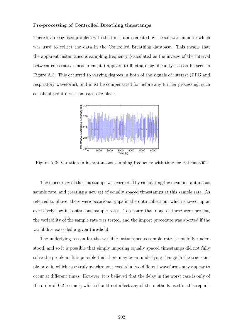
Pre-processing of Controlled Breathing timestamps

There is a recognised problem with the timestamps created by the software monitor which

was used to collect the data in the Controlled Breathing database. This means that

the apparent instantaneous sampling frequency (calculated as the inverse of the interval

between consecutive measurements) appears to fluctuate significantly, as can be seen in

Figure A.3. This occurred to varying degrees in both of the signals of interest (PPG and

respiratory waveform), and must be compensated for before any further processing, such

as salient point detection, can take place.

0 1000 2000 3000 4000 5000 6000220

240

260

280

300

Time (s)

Inst

anta

neou

s sa

mpl

ing

freq

uenc

y (H

z)

Figure A.3: Variation in instantaneous sampling frequency with time for Patient 3002

The inaccuracy of the timestamps was corrected by calculating the mean instantaneous

sample rate, and creating a new set of equally spaced timestamps at this sample rate. As

referred to above, there were occasional gaps in the data collection, which showed up as

excessively low instantaneous sample rates. To ensure that none of these were present,

the variability of the sample rate was tested, and the import procedure was aborted if the

variability exceeded a given threshold.

The underlying reason for the variable instantaneous sample rate is not fully under-

stood, and so it is possible that simply imposing equally spaced timestamps did not fully

solve the problem. It is possible that there may be an underlying change in the true sam-

ple rate, in which case truly synchronous events in two different waveforms may appear to

occur at different times. However, it is believed that the delay in the worst case is only of

the order of 0.2 seconds, which should not affect any of the methods used in this report.

202

Pre-processing of Controlled Breathing respiratory waveform

The raw respiratory waveforms in the Controlled Breathing database were very noisy,

and also had widely varying breath amplitudes due to the differing tidal volumes defined

in the experimental protocol. Simple automated techniques proved to be insufficiently

accurate, and so a method combining automatic detection with manual intervention was

devised in order to save time.

The raw respiratory waveform was first filtered using a band-pass filter with the pass-

band from 0.1–0.7 Hz (6–42 breaths/minute). The filter was designed using a Kaiser

windowing function, with 5% ripple in the pass-band, 20dB attenuation at low frequencies,

and 30dB attenuation at high frequency. The order of the digital filter was limited to

ensure that the delay does not exceed 5 seconds.

0 200 400 6001.675

1.68

1.685

1.69

1.695

1.7x 104

Time (s)

(a) Original respiratory waveform

0 200 400 600−80

−60

−40

−20

0

20

40

60

80

Time (s)

(b) Filtered and detrended respiratory wave-form

Figure A.4: Original and filtered versions of the respiratory waveform for Patient 3002in the the Controlled Breathing database, with the detected breaths (using manual inter-vention) shown in red.

The filtered signal was then detrended to remove any remaining dc offset, and the zero-

crossings algorithm described in Section B.2 was used to identify peaks in the signal. The

user chooses a window size (in seconds) and an overlap between consecutive windows. The

algorithm then presents the user with the first window length of signal (filtered respiratory

waveform), with the identified peaks shown, and prompts the user for a threshold for the

window. The result of the threshold is previewed, allowing the user to accept the threshold

or enter a new one. Once a threshold is accepted, any peaks that lie within the window

203

and below the threshold are removed from the list of peaks, and the user is presented

with the next window of data from the signal.

Pre-processing of Controlled Breathing PPG waveform

During initial attempts to obtain respiratory rate from the Controlled Breathing PPG

waveform, it was observed that many of the records showed significant baseline variations

at frequencies much lower than breathing. The causes of these variations are not known,

but may include movement artefact, varying light levels and intrinsic properties of the

sensor hardware.

The difficulty of removing this variation lies in the fact that the wanted breathing

signal will also cause low frequency variations in the baseline, and we do not want to

remove this signal in the pre-processing stage. A cut-off frequency of around 0.005 Hz

(0.3 breaths/minute) was chosen, to ensure that no breathing signals would be removed,

but with the knowledge that this would not remove all of the artefactual low frequency

signals.

It was decided that a digital filter would not be an appropriate method for this problem,

as the cut-off frequency would be very low in comparison to the sampling frequency

(about 81 Hz), and the transition band would have to be quite narrow to ensure that all

physiologically plausible respiratory rates lay in the pass-band. An alternative method

using cubic splines was therefore devised, and is demonstrated in Figure A.5.

The raw PPG signal was first detrended, and then downsampled to 0.01 Hz (so that

the Nyquist frequency is equal to the defined cut-off frequency of 0.005 Hz). It was

impractical to use decimation for such a large downsampling ratio, so one decimation

step was used to downsample by a factor of 10, and then all further downsampling was

done without any additional filtering.

A cubic spline was fitted to the downsampled waveform, and interpolated to the orig-

inal sampling rate. This signal was then subtracted from the detrended original signal to

give the pre-processed signal. As can be seen from Figure A.5, the pre-processed signal

still has some artefactual baseline variation, but this is much less than that seen in the

original signal.

204

0 500 1000 1500 2000 2500 3000 3500

2

2.2

2.4x 10

4

original

0 500 1000 1500 2000 2500 3000 3500

−2000

0

2000

detrendedresampledspline

0 500 1000 1500 2000 2500 3000 3500

−2000

0

2000

Time (s)

output

Figure A.5: Pre-processing of PPG waveform from patient 3010 in the Controlled Breath-ing database

205

A cut-off frequency of 0.005 Hz was appropriate for pre-processing prior to analysis

of amplitude modulation, as it was important not to remove any amplitude-modulated

information in the signal. However, the residual baseline variation after this level of pre-

processing was still too great to allow accurate peak detection, which was required for

analysis of frequency modulation of the PPG. The PPG was therefore pre-processed with

a higher cut-off frequency of 0.05 Hz prior to the detection of salient points for analysis

of frequency modulation of the PPG.

A.1.3 Paediatric data from Oxford School Study

The Oxford School study dataset contains data measured using Visi-3 systems from 36

children (16 female, 20 male) between the ages of 8 and 11 years, with a mean age of 9.9

years. Details of the measurement procedure are given in Section 5.1.1.

Pre-processing of the Visi-3 waveforms

The raw exported Visi-3 waveforms contained artefacts at the end of the recording that

should be removed prior to analysis, as they consisted of a large step in value which might

confuse the analysis algorithms. An example of the artefact on a nasal airflow waveform

is shown in the top graph in Figure A.6, although it should be noted that the artefact

appears on all the respiratory and PPG waveform recordings.

465 470 475 480−2

0

2

4x 10

4

Raw

wav

efor

m

465 470 475 480−2000

0

2000

4000

Art

efac

t rem

oved

Time (s)

Figure A.6: Removal of artefact at the end of a Visi-3 recording of nasal airflow

The artefact is identified using the gradient of the raw waveform, as the step in value

occurs in a single sample (i.e. there are no intermediate samples on the upslope), and

is followed by a completely flat section with a gradient of zero. Therefore, the position

206

of the step is identified as the last non-zero sample-to-sample gradient in the recording.

Rather than removing the artefactual values, they are replaced by the value of the last

sample before the step function, as shown in the lower graph in Figure A.6.

In addition to the artefact at the end of the recording, the PPG waveforms from the

Visi-3 system also contain artefacts at the beginning of the recording, as demonstrated

in the top graph in Figure A.7. These artefacts are only present on the PPG waveforms,

and appear at approximately the same point in the recording (between 5 and 6 seconds

from the start).

0 5 10 15−2

0

2x 10

4

Raw

wav

efor

m

0 5 10 15−5000

0

5000

Art

efac

t rem

oved

Time (s)

Figure A.7: Removal of artefact at the start of a Visi-3 PPG waveform

The artefacts at the beginning of the PPG signal were removed using knowledge about

where they appear. The value of the signal at 4 seconds from the start of the recording

was taken as a ‘non-artefact’ value, as the artefact always appeared at or around 5 seconds

from the start. The artefact was deemed to be over when 6 seconds had elapsed from the

start of the recording and the value of the signal was greater than or equal to the ‘non-

artefact’ value found earlier. The period of the artefact was replaced by the ‘non-artefact’

value, as shown in Figure A.7.

Breath detection on Visi-3 respiratory waveforms

The breath detection algorithm described in Section B.2 proved to be insufficiently accu-

rate for use on the Visi-3 reference respiratory waveforms, due to the wide possible range

of respiratory rates, and the large amounts of noise present on some of the waveforms. A

new method was therefore developed to deal with these waveforms.

As shown in Figure A.8, the respiratory waveforms were filtered prior to breath detec-

207

10 15 20 25 30 35 40−5000

0

5000

10000

orig

inal

10 15 20 25 30 35 40−5000

0

5000

filte

red

Time (s)

(a) Nasal airflow

10 15 20 25 30 35 40−5000

0

5000

orig

inal

10 15 20 25 30 35 40−2000

0

2000

filte

red

Time (s)

(b) Thoracic effort

Figure A.8: Filtering of Visi-3 respiratory waveforms prior to breath detection

tion. This was particularly important for some of the respiratory effort waveforms, which

had high frequency components which mostly obscured the respiratory signal. These were

only seen with one of the Visi-3 systems, and it was hypothesised that they were due to

the high frequency signal used to assess the inductance of the respiratory effort band.

A FIR low-pass filter using the Kaiser windowing function was used. The transition

band of the filter was set to be 1.7–2.5 Hz (102–150 breaths/minute), with a 5% pass-band

ripple and 30 dB of attenuation in the stop-band. The filtered waveform was detrended

to remove any d.c. offset. As with the method described previously, peaks in each of the

three waveforms were identified using the zero-crossings of the point-to-point gradient.

As these respiratory waveforms contained large amounts of noise and artefact, the

results of this peak detection on any one of the three individual waveforms was insuffi-

ciently accurate to be used as a source of reference respiratory information. This was due

in part to extra or missed breaths in the peak detection, but also because of periods of

poor quality signal which could affect any of the three channels from time to time.

Since all children had at least two reference respiratory waveforms recorded (from

the two effort bands), it was hypothesised that the temporal correlation between the

waveforms could be used to differentiate true breaths from artefactual peaks. Since a

period of poor signal quality could cause one of the three waveforms to fail to register a

breath, and as some children did not wear the nasal cannulae for the full length of the

recording, it was decided that correlation between at least two of the three waveforms

should be regarded as sufficient to identify a peak as a true breath.

Both the filtering procedure and the additive noise on the waveforms can cause distor-

208

tion of the signal, resulting in the detected peak being shifted in time between waveforms.

In addition, there may not necessarily be perfect temporal correlation between the three

waveforms due to temporal delays between the corresponding physiological processes that

are being measured.

All of the detected peaks (from all of the waveforms) were sorted in time, and a window

of one second was therefore used to determine if two peaks were co-incident, and thus

could be identified as a true breath. If two consecutive peaks from different waveforms

occurred within a one-second window, the mean time of the two peaks was taken as the

time of the corresponding breath.

This algorithm allows for a given peak to participate in two ‘breaths’ (paired with both

the preceding and following peak if both are from different waveforms and are within the

one-second window). The initial list of breaths must therefore be cleaned to ensure that

peaks only participated in a single breath, and, where necessary, to combine data from

peaks in all three waveforms into a time for a single breath. This process was carried

out by identifying ‘chains’ of breaths, where each breath shared at least one peak with

another breath. The algorithm applied for handling each chain depended on the number

of peaks in the chain.

Pattern Algorithm ResultABC single breath ABC

A1BA2 A1B < BA2 A1BA1B > BA2 BA2

Table A.3: Algorithm for handling chains containing three peaks (two linked breaths)

For chains containing three peaks (two linked breaths), there are two possible scenarios,

outlined in Table A.3, where A, B and C refer to the three possible waveforms from which

the peaks could have originated. The time between the peaks was used as a measure of

distance to decide which possible result to choose, where multiple results were possible,

as with the pattern A1BA2.

When a chain contained four peaks (three linked breaths), the options became more

numerous, as shown in Table A.4. For longer chains, the first four peaks were dealt with

as shown in Table A.4, and then the last grouping resulting from this (e.g. A2C from the

second row, or the removed B2 from the sixth option) was combined with further peaks

209

Pattern Algorithm ResultA1B1A2B2 two breaths A1B1, A2B2

A1BA2C A1B < BA2 A1B, A2CA1B > BA2 BA2C

A1BCA2 A1B < CA2 A1BCA1B > CA2 BCA2

AB1CB2 B1C < CB2 AB1CB1C > CB2 AB1, CB2

Table A.4: Algorithm for handling chains containing four peaks (three linked breaths)

from the chain, and the process was repeated iteratively until no more peaks remain in

the chain.

60 65 70 75 80 85 90−2000

0

2000

4000Nasal Airflow

60 65 70 75 80 85 90−1000

0

1000

2000Thoracic Effort

60 65 70 75 80 85 90−1000

0

1000Abdominal Effort

Time (s)

Figure A.9: Example of peak matching to detect breaths in data from Oxford SchoolStudy. Matched peaks are shown in red, unmatched peaks are shown in black. Thepositions of detected breaths are plotted in magenta.

This method performed well on most of the reference breathing data from the Oxford

School Study, as can be seen in Figure A.9. However, there were some periods of data

where the waveforms showed extremely noisy signals, resulting in large numbers of spu-

rious peaks, some of which fall within the one-second window despite the fact that they

are unlikely to correspond to true breaths. Most of these signals were difficult to anal-

yse manually, and were thought to correspond to periods of time when the experimental

subjects were talking. An example of this type of data is shown in Figure A.10. As an

accurate reference respiratory rate cannot be calculated for these records, they have been

excluded from the analysis in this thesis.

210

0 5 10 15 20 25 30−5000

0

5000

10000Nasal Airflow

0 5 10 15 20 25 30−2000

0

2000Thoracic Effort

0 5 10 15 20 25 30−4000

−2000

0

2000Abdominal Effort

Time (s)

Figure A.10: Example of poor data quality causing failed peak matching in referencebreathing data from Oxford School Study. Matched peaks are shown in red, unmatchedpeaks are shown in black. The positions of detected ‘breaths’ are plotted in magenta.

A.1.4 Paediatric data from OXEMS Study

The OXEMS study dataset contains data measured from 52 children between the ages of

one month and ten years, with a median age of 2.8 years. The dataset contains photo-

plethysmogram (PPG) waveforms recorded from a Bluetooth pulse oximeter, along with

associated heart rate, oxygen saturation and peripheral perfusion values. Manual mea-

surements of respiratory rate were also available for 44 children (the subset considered in

this thesis), and at least one axillary temperature was recorded for 47 children.

Pre-processing of OXEMS PPG waveform timestamps

The timestamps for the PPG waveform in the OXEMS dataset each correspond to a

‘packet’ of data containing 25 samples of the waveform. As the nominal sample rate of

the PPG waveform is 75 Hz, the gap between these timestamps should ideally not exceed

one third of a second. However, many of the records contained significant gaps, which

may exceed ten seconds in length. The cause of these gaps is not known, although it was

hypothesised that some of the longer gaps are due to probe disconnections or problems

with Bluetooth connectivity.

It was observed that a number of records contained very long gaps just preceding the

211

end of the recording. These were likely to correspond to records where the recording was

not manually closed, and was ended by the entry of a new patient. If this new patient

was connected to the pulse oximeter before the old record was closed, this would explain

the short period of PPG recorded following the gap. From observation of the waveforms,

a threshold of 70 seconds was set to identify this type of gap. Waveforms containing

a gap exceeding this threshold were truncated, so that the end of the waveform record

corresponded to the beginning of the gap. This truncation step was applied to 22 of the

44 records of interest.

One option investigated for dealing with the shorter gaps was to pad the waveform

with the last known value (sample and hold). However, this did not prevent step changes

in value occurring at the end of the gap, which could cause problems for signal analysis

methods. It was also observed that the signals on either side of many of the gaps appeared

to ‘join up’ without step changes, supporting the theory that the gaps in timestamps may

have been due to Bluetooth connectivity issues, and that there was, in fact, often no

loss of the underlying data. It was therefore decided that padding the waveform was

inappropriate, and that reconstructing the time vector at the nominal sample rate would

be a better solution to the problem.

It should be noted that this reconstruction method is likely to result in PPG waveforms

which contain a small number of discontinuities, where gaps that correspond to true loss

of data are compressed so that the waveforms on either side of the gap abut each other.

However, it is believed that the number of this type of gap is very small, and so the impact

on further processing of the PPG waveform should be slight.

A.2 Paediatric vital signs data from primary and emer-

gency care

Two datasets from primary and emergency care were used to develop and test the data

fusion algorithms. These are the Fever and Tachycardia (FaT) dataset, collected from

children with fever in primary care; and the Walsgrave dataset, collected from children

with suspected acute infection admitted to a paediatric assessment unit.

212

A.2.1 The Fever and Tachycardia dataset

The Fever and Tachycardia (FaT) dataset was collected as part of a study to assess the

amount by which the presence of fever increases a child’s heart rate (Thompson et al.,

2009b). It was collected from children presenting with fever to 10 GP surgeries in Ox-

fordshire, Buckinghamshire and Somerset, and 2 out-of-hours GP centres in Oxfordshire,

between December 2003 and March 2006.

The dataset used in this study consisted of 1941 children with measurements of both

axillary temperature and heart rate. Of these, 873 children (45%) also had their SpO2

measured using a pulse oximeter.

The severity of illness was assessed by checking for hospital admission in the 7 days

following the child’s assessment. Of the 1941 children included in the dataset, 43 (2.2%)

met this definition of serious illness.

A.2.2 The Walsgrave dataset

The Walsgrave dataset was collected from children attending the Paediatric Assessment

Unit (PAU) at University Hospital Coventry and Warwickshire NHS trust (Thompson

et al., 2009a). Children were recruited if an acute infection was suspected. Exclusion

criteria included infection due to penetrating trauma, and pre-existing conditions such as

haematological malignancies or immunosuppression, which would predispose the children

to repeated serious bacterial infections.

The dataset used in this study consisted of 681 children with measurements of both

axillary temperature and heart rate. Of these, 664 children (97.5%) also had their SpO2

measured using a pulse oximeter, and 568 children (83.4%) had both SpO2 measurements,

and a manual measure of respiratory rate.

The children in this study were categorised by the presence and severity of infection.

We used the presence of serious infection as a marker, defined as an infection which is

likely to be life-threatening if left untreated, or with a high chance of life-threatening

complications or sequelae. Of the 681 children in the dataset, 106 (15.6%) were given this

classification.

213

A.2.3 The combined FW dataset

The data from both the FaT and Walsgrave datasets were combined to form a larger

dataset of 2622 children, all of whom have measurements of both heart rate and temper-

ature, and some of whom also have measurements of SpO2 and respiratory rate.

One issue with the FW dataset is that there is inconsistency in the classification of

serious illness, in that some of the ‘non-serious’ children in the Walsgrave dataset would

be classified as ‘serious’ in the FaT dataset.

A.2.4 Using the datasets for data fusion

For the purposes of developing data fusion algorithms, it was useful to create datasets

with consistent numbers of variables. Therefore, the datasets described in this section

were split into subsets containing 2, 3, or 4 vital signs, as shown in Table A.5.

Number of Dataset Vital Signsvital signs FW FaT Walsgrave HR Temp SpO2 RR

2 2622 (149) 1941 (43) 681 (106) • •3 1537 (132) 873 (28) 664 (104) • • •4 0 0 568 (93) • • • •

Table A.5: Contents of datasets used for data fusion. Numbers in brackets are childrenclassified as having serious illness

The seven datasets described in Table A.5 were used for testing data fusion methods.

Individual datasets are referred to by the name of the superset followed by the number

of vital signs in the dataset (e.g. Walsgrave4 or FW3).

It is interesting to note that the percentage of children classified as having serious ill-

ness increases as more vital signs are measured. It is likely that this was due to recognition

of serious illness by clinicians, who were then more likely to measure extra vital signs, as

they were perceived to be of greater utility in serious illness. It should be noted however,

that of the 149 children in the FW2 dataset who were classified as having serious illness,

17 (11.4%) did not have their SpO2 measured. Even in the PAU setting, where almost all

of the children had measurements of SpO2 and the vast majority had measurements of

respiratory rate, 2 out of 106 children (1.9%) classified as seriously ill did not have their

SpO2 measured, and 13 (12.3%) did not have their respiratory rate measured.

214

Appendix B

Mathematical Methods

This appendix brings together the theoretical basis behind some of the algorithms and

mathematical methods that are used in this thesis.

B.1 Kernel regression

Kernel regression is a non-parametric regression method, which allows a curve to be fitted

to a set of data without specifying the form of the curve in advance.

To fit curves to the data on heart rate and respiratory rate in relation to age in

children, it would be beneficial to have a regression method that could take into account

the different age ranges over which the measurements had been made, and would also

allow weighting based on the sample size. No existing regression method was found that

allowed for these variables, but it was possible to make simple alterations to the classical

formulation of kernel regression to incorporate these changes.

This section explains the standard kernel regression method, and then covers the

alterations made to this method for use in fitting curves to the data on heart rate and

respiratory rate in relation to age in children.

B.1.1 Classic kernel regression

In kernel regression, a kernel K(x) is centred on each data point, x = Xi. Typically, the

kernel will be unimodal, symmetric about zero, and satisfy∫

K(x)dx = 1, such that it is

a valid probability density function. A popular choice for K(x) is the normal distribution

215

with zero mean and unit variance, and this is what was used as the definition of K(x) in

this thesis, as shown in Equation B.1.

K(x) =1√2π

exp

(−x2

2

)= N(0, 1) (B.1)

The kernel defines the spatial weighting given to the data point in the regression. Far

away from the data point, the kernel function will have a small amplitude, and so the

point will only make a small contribution to the regression curve, whereas it will make a

large contribution in the region close to its location, where the value of the kernel function

is larger. The width of the kernel function can be altered to control the smoothness of

the final curve – this is controlled by the bandwidth h, and can be incorporated into the

definition of the kernel by a change of variables as shown in Equation B.2.

Kh(u) =1

hK

(u

h

)(B.2)

Large values of bandwidth will produce smooth curves, as each point will contribute

to a large portion of the curve. Smaller values will produce more noisy curves, and are

more likely to exhibit overfitting to the data, as each data point only affects a small

portion of the curve, and does not share influence over a given section with many other

points. Figure B.1 shows how a range of bandwidth values lead to over-smoothed and

under-smoothed curves for a given set of data points.

We will consider local polynomial kernel regression, which operates by fitting a poly-

nomial at each point on the curve, weighted by the values of the kernels at that point.

The degree of the polynomial fitted is denoted by p, so p = 1 would fit a straight line at

each point. If h = ∞, the kernel regression will tend to a simple polynomial fit to the

data.

To calculate the value of the kernel regression estimator m(x; p, h) at point x, a poly-

nomial of order p, as shown in Equation B.3, is fitted using weighted least squares. The

weights are determined by the kernel weights Kh(Xi − x), where (Xi, Yi) are the data

points, and βn are the polynomial co-efficients to be determined.

Yi = β0 + β1(Xi − x) + . . . + βp(Xi − x)p (B.3)

216

0 1 2 3 4 5 6 7 8−5

0

5

10

15

20

25

x

y

datah=1h=0.4h=0.05

Figure B.1: Effect of changing the bandwidth in kernel regression

The value of m(x; p, h) is the height of the fit, β0, where β = (β0, . . . , βp)T minimises

n∑

i=1

Yi − β0 − . . .− βp(Xi − x)p2 Kh(Xi − x),

where n is the number of data points from which the regression curve will be calculated.

In this thesis, we deal only with the cases where p = 0 and p = 1, for which there

are simple explicit formulae. However, for higher values of p, it is necessary to use more

complex calculations involving matrix inversion, more details of which may be found in

Wand and Jones (1995). In the case of p = 0, the Nadaraya-Watson estimator, given in

Equation B.4 may be used.

m(x; 0, h) =

∑ni=1 Kh(Xi − x)Yi∑ni=1 Kh(Xi − x)

(B.4)

When p = 1, the explicit formula for the local linear estimator is used, as given in

Equation B.5, where sr is given by the formula in Equation B.6.

m(x; 1, h) =1

n

n∑

i=1

s2(x; h)− s1(x; h)(Xi − x)Kh(Xi − x)Yi

s2(x; h)s0(x; h)− s1(x; h)2(B.5)

217

sr =1

n

n∑

i=1

(Xi − x)rKh(Xi − x) (B.6)

The choice of p is determined by a number of factors. Increasing p naturally increases

the computational complexity of the estimation, but also increases the ability of the

estimator to follow large changes in gradient. The behaviour of the estimator at the

boundaries of the data can also be a major factor, as the form of the curve will tend towards

that of the underlying polynomial at the boundaries. So, for example, an estimator with

p = 0 will tend towards a horizontal line at its boundaries, whereas one with p = 1 will

tend towards a straight line, but not necessarily one with a gradient of 0.

B.1.2 Weighted variable bandwidth kernel regression

When fitting curves to the data on heart rate and respiratory rate in relation to age in

children, each data point is associated with an age range, rather than a single age, as the

measurements have been made on groups of children. The size of the ranges can vary

greatly, with some studies focusing on children grouped into year groups, while others

may use 5-year groups, especially when considering older children.

One possible solution to this problem was to assign the data to the mid-point of the

range, but this ignores the fact that it contains information about both older and younger

children. It also complicates the estimation of the variance, as a larger measured age

range will have a larger expected variance.

It was therefore preferable to include the age range in the regression calculation, and

this could be achieved using variable bandwidth kernel regression. In this formulation

of kernel regression, h is replaced by hi, so that the kernel centred on each data point

is now able to have an independent bandwidth. The value of hi at for each data point

was calculated using Equation B.7, where ∆Xi is the age range associated with the data

point, and hc is a common multiplier which allows the overall smoothing of the curve to

be manipulated.

hi = hc∆Xi (B.7)

218

In addition to including variable bandwidths, it would also be useful to add weighting

to data points to reflect the sample sizes of the measurements from which they are derived.

This could be achieved by adding a weighting term wi to the kernel function, such that the

resulting kernel function Khiis as shown in Equation B.8. The value of wi for each data

point was equal to the sample size for that point. This definition for the kernel function

could then be used in place of Kh in the Nadaraya-Watson or local linear estimator

equations (Equations B.4 and B.5).

Khi(u) =

wi

hi

K(

u

hi

)(B.8)

B.2 Simple breath detection algorithm

Automated breath detection was used to calculate respiratory rates from the reference

breathing waveforms, as well as being required by some of the techniques in Chapter 4.

The algorithm described here was based on one described in Mason (2002), although a

number of modifications have been made to improve the accuracy of the results. Despite

its simplicity, it has been found to be quite robust to noise on the breathing waveform.

The algorithm is based on extrema detection, which allows the timestamps of individ-

ual breaths to be extracted. An extremum (peak or trough) is valid if the following four

rules are met:

1. The appropriate change in gradient has occurred (from positive to negative for a

peak, or negative to positive for a trough)

2. The extremum is of the opposite type to that of the last detected extremum (i.e. a

trough must be followed by a peak and vice versa)

3. The signal value at the extremum is above the mean for a peak, and below the mean

for a trough

4. The distances to the previous and next extrema of the same type must both be

greater than a specified minimum delay

219

The changes in the gradient of the signal were detected by finding the zero-crossings of

the point-to-point gradient. Identifying points where the signal changes sign is relatively

trivial. However, if the signal passes through zero, it is necessary to check that the signal

has changed sign for a crossing to be identified. To do this, the two surrounding non-zero

points were identified and checked. This also allowed identification of the sign of the slope

at the zero crossing, which assists in the implementation of Rule 1.

Once peaks and troughs had been identified using the zero-crossings, further processing

was then used to remove peaks and troughs that did not comply with Rules 3 or 4, while

ensuring that Rule 2 still holds. The mean value of the signal was calculated as a rolling

mean, with a window equal to 150 times the minimum delay specified in Rule 4. This

should ensure that changes in the baseline of the signal (either through baseline drift

or step changes) are tracked and did not adversely affect the accuracy of the algorithm.

For most of breathing-synchronous waveforms examined in this report, Rule 4 was not

required, as Rules 1–3 tended to remove all invalid extrema.

Figure B.2 shows the detection of breaths from a MIMIC respiratory waveform con-

taining artefacts. As the breaths were detected after filtering as described in Section A.1.1,

the positions of the detected breaths correspond to the peaks in the filtered waveform.

These may be slightly different from the positions of the peaks in the original waveform,

as the low pass filtering will tend to reduce any asymmetry in the shape of the peaks.

After detection, the detected breath positions were checked visually to ensure that all

of the breaths in the respiratory waveform were identified, and that all of the detected

breaths corresponded to actual breaths in the waveform.

B.3 Autoregressive modelling

Autoregressive (AR) modelling is a frequency-based signal analysis technique, which was

used in this thesis as a way of identifying the frequency of a periodic physiological signal

(e.g. respiratory rate).

AR modelling can be formulated as a linear prediction problem, where the current

value x(n) can be modelled as a linearly weighted sum of the preceding p values. The

parameter p is the model order, which is usually much smaller than the length of the

220

40 50 60 70 80 90−0.6

−0.4

−0.2

0

0.2

0.4

Time (s)

mV

Figure B.2: Breath detection (red stars) on a respiratory waveform with artefacts fromthe MIMIC database. The original waveform is shown in blue, with the waveform usedfor detection (after artefact removal and filtering) in green.

sequence N .

x(n) = −p∑

k=1

akx(n− k) + e(n) (B.9)

The value of the output x(n) is therefore a linear regression on itself, with an error

e(n), which is assumed to be normally distributed with zero mean and a variance of σ2.

The problem can also be visualised in terms of a system with input e(n), and output x(n),

in which case the transfer function H can be formulated as shown below:

H(z) =1∑p

k=0 akz−k=

zp

(z − z1)(z − z2) . . . (z − zp)(B.10)

As shown in Equation B.10, the denominator of H(z) can be factorised into p terms.

Each of these terms defines a root zi of the denominator of H(z), corresponding to a

pole of H(z). Since H(z) has no zeros away from the origin, the AR model is an all-pole

model. The poles occur in complex-conjugate pairs, and define spectral peaks in the power

spectrum of the signal, with higher magnitude poles corresponding to higher magnitude

peaks. The resonant frequency of each spectral peak is given by the phase angle of the

corresponding pole.

The phase angle θ corresponding to a given frequency f is defined by Equation B.11,

which shows that it is also dependent on the sampling interval ∆t.

θ = 2πf∆t (B.11)

221

B.4 Kalman filtering

A Kalman filter uses probabilistic reasoning to produce an estimate x of the state x based

on measurements z. It can also be used for data fusion of multiple measurements.

The true state x is assumed to evolve as shown in Equation B.12. The equations

presented here will be in the general multi-dimensional matrix form, but can be simplified

in the one-dimensional case.

xk = Axk−1 + wk w ∼ N(0,Q) (B.12)

The state transition matrix, A, defines how the state evolves over discrete time in-

tervals. The process noise, w describes the noise in the true state, and is assumed to be

normally distributed with zero mean and covariance Q. If we know the true value of x for

some of our measurement data, we can estimate an appropriate value for Q by calculating

the actual process noise, w = xk − xk−1, and observing its statistics.

The evolution of the measurement, z, is expected to conform to Equation B.13, where

H is the observation matrix, which describes the relationship between the measurements

and the true state. The measurement noise, v, is expected to be normally distributed

with zero mean and covariance R. As with the process noise covariance, we may be able

to estimate an appropriate value for R by observing the statistics of the error vector.

zk = Hxk + v v ∼ N(0,R) (B.13)

At each step, the Kalman filter calculates values for the state estimate x and its

covariance P. The initial values x0 and P0 need to be supplied to the algorithm, and

appropriate estimates can be calculated by finding the mean and variance of known values

of x. At each time-step, new values of x and P are calculated using Equations B.14 and

B.15.

xk = Axk−1 (B.14)

Pk = APk−1AT + Q (B.15)

222

From these initial estimates, the Kalman gain K is calculated, and is used to update

the initial estimates, as shown in Equations B.16–B.18.

Kk = PkHT(HPkH

T + R)−1 (B.16)

xk = xk + Kkzk (B.17)

Pk = Pk −KkHPk (B.18)

B.5 Probabilistic principal component analysis

Probabilistic principal component analysis (PPCA) allows a general Gaussian density

model to be calculated based on the principal component decomposition of a set of data

(Tipping and Bishop, 1999; Nabney, 2002). This density model allows calculation of the

probability density at a new data point, tnew. In Chapter 5, extreme value theory (Section

B.6) was applied to the calculated probability density, in order to obtain a measure of the

novelty of the new data point. This combination of PPCA and extreme value theory was

then used to identify poor quality sections of PPG waveform.

Principal component analysis is a form of dimensionality reduction, where the original

d-dimensional data, tn, is reduced to q-dimensional transformed data, xn, where q < d.

Equation B.19 shows the transformation from the data space to the principal component

space, where Uq = (w1,w2, . . . ,wq) is the matrix of the principal axes, and t is the mean

value of the training data.

xn = UTq (tn − t) (B.19)

To maximise the retained variance under projection, the sample covariance matrix, S,

of the training data is calculated. The principal axes are then defined as the q dominant

eigenvectors of S, which have the largest eigenvectors, λi, as shown in Equation B.20.

This projection minimises the squared reconstruction error when tn is reconstructed from

223

xn using Equation B.21.

Swj = λjwj (B.20)

tn = Uqxn + t (B.21)

Reconstruction of t using Equation B.21 will not be exact. Equation B.22 shows that

the linear reconstruction of d-dimensional data from a q-dimensional model will include

an error term ε. In this equation, W is a d× q matrix relating the two sets of variables,

and µ permits the model to have a non-zero mean.

t = Wx + µ + ε (B.22)

Conventionally, x ∼ N(0, I), so that the latent variables x are independent, Gaussian-

distributed, and with unit variance. If the error vector is also modelled with a Gaussian

distribution: ε ∼ N(0,Ψ), then the distribution of the observed data, t, is as shown in

Equation B.23.

t ∼ N(µ,WWT + Ψ) (B.23)

In probabilistic principal component analysis, the distribution of ε is assumed to be

an isotropic Gaussian, such that the error covariance, Ψ, is diagonal: Ψ = σ2I.

The maximum likelihood estimator for µ is given by the sample mean of the data.

Maximum likelihood estimators for W and σ2 are shown in Equations B.24 and B.25. In

Equation B.24, Uq is the matrix of the dominant q eigenvectors, as described earlier, and

Λq are the corresponding eigenvalues. R is an arbitrary orthogonal rotation matrix, and

is usually taken to be the identity matrix: R = I.

WMLE = Uq(Λq − σ2I)1/2R (B.24)

The maximum likelihood estimator for σ2, shown in Equation B.25, can be interpreted

as representing the ‘lost’ variance due to projecting the data into a lower dimensional

224

space.

σ2MLE =

1

d− q

d∑

j=q+1

λj (B.25)

The observed data may therefore be modelled as t ∼ N(µ,WWT + σ2I), where the

values of µ, W, and σ2 are determined by the maximum likelihood estimators described

above. By considering the probability density of this distribution, new data points can

be assessed to determine whether they are novel with respect to the training data used

to derive the model parameters.

B.6 Novelty detection using multivariate extreme value

theory

Extreme value theory describes the behaviour of the extreme value (smallest/largest) in

a set of data. This will tend to lie away from the median of the probability distribution

associated with the data (i.e. in the tails of the distribution). Extreme value theory can

be used to determine the “normality” or “novelty” of the extreme value of a set of data

points, when compared to a model of normality created using examples of “normal” data.

In Section 5.4, multivariate extreme value theory was used to perform novelty detection

of sections of PPG waveform, in order to identify periods of poor quality signal.

Classically, extreme value theory is applied to univariate distributions. Clifton et al.

(2010) extend this to multivariate distributions, and demonstrate how it can be applied to

the problem of novelty detection. This appendix summarises the theory in Clifton et al.

(2010) as it pertains to the application in Chapter 5.

We assume that a set of data has been drawn from a unimodal, n-dimensional Gaussian

distribution, fn(x), which has the form given in Equation B.26. In this equation, M(x)

is the Mahalonobis distance defined in Equation B.27, Cn is the normalisation coefficient

defined in Equation B.28, µ is the centre of the distribution, and Σ is the covariance

matrix.

225

fn(x) =1

Cn

exp

(−M(x)2

2

)(B.26)

M(x) =((x− µ)TΣ−1(x− µ)

)1/2(B.27)

Cn = (2π)n/2|Σ|1/2 (B.28)

If m samples, x1,x2, . . . ,xm, are drawn from this distribution, they will have the

corresponding pdf values, fn(x1), fn(x2), . . . , fn(xm). Samples with a low value of fn

correspond to extrema (i.e. they are in the tails of the distribution). We can therefore

reduce the problem to one dimension by considering the distribution of probability density

values. The probability of a given probability density value, P (fn(x)) = Gn(y), where

y = fn(x). Clifton et al. (2010) show that the distribution Gn can be defined as shown

in Equation B.29, where Ω is as defined in Equation B.30, and Γ refers to the Gamma

function. Clifton et al. (2010) provide analytical solutions for this integration for odd and

even values of n.

Gn(y) = Ω|Σ|1/2∫ y

0[−2 ln(Cnu)](n−2)/2du (B.29)

Ω =2πn/2

Γ(n2)

(B.30)

To apply extreme value theory to Gn, we require the corresponding probability distri-

bution function gn(y), defined in Equation B.31. Applying extreme value theory results

in the Weibull extreme value distribution, Gen(y), given in Equation B.32.

gn(y) = Ω|Σ|1/2[−2 ln(Cny)](n−2)/n (B.31)

Gen(y) = 1− exp

(−

(y

cm

)αm)

(B.32)

In Equation B.32, cm is the scale parameter, and can be estimated from Equation

226

B.33, which defines cm as the 1m

th quantile of Gn. The shape parameter αm is estimated

using Equation B.34.

cm = G←n

(1

m

)(B.33)

αm = cmgn(cm)

Gn(cm)(B.34)

To obtain a novelty score using extreme value theory, we consider the probability of

drawing m samples of data whose extremum has a higher probability than that observed in

the samples under consideration. This probability, F en(x) = 1−Ge

n(ym), so our extremum

is abnormal with probability 1−Gen(ym). As suggested in Clifton et al. (2010), we define

our novelty score as in Equation B.35. This novelty score was used in Section 5.4 to assess

the signal quality of sections of PPG waveform.

Z(xM) = − ln (1− F en(xM)) (B.35)

B.7 Pruning of outliers using GMMs

Before building some of the data fusion models described in Chapter 6, it was helpful

to remove obvious outliers to avoid overfitting of the model to the data. One method,

developed by Dr David Clifton, for achieving this is using Gaussian mixture models, and

is described here.

−10 −5 0 5 10−10

−5

0

5

10

Figure B.3: Example dataset with outliers

An example dataset is shown in Figure B.3. This dataset was created using samples

227

from two Gaussian kernels as well as four manually added outlier points. The outlier

removal process is carried out in two steps.

−10 −5 0 5 10−10

−5

0

5

10

(a) Results from initial pruning step

−10 −5 0 5 10−10

−5

0

5

10

(b) Results from final pruning step

Figure B.4: Pruning of outliers using GMMs. GMM centres are shown in green. Prunedpoints (outliers) are shown in blue, with retained points shown in red.

In the first step, a simple Gaussian mixture model is fitted to the data. The model

uses three spherical kernels, and 20 training iterations. The centres of the resulting kernels

are shown by the large green stars in Figure B.4(a). The probability density p(xi) of each

data point in the data set is calculated, and the value of p(x) at which the probability

P (p(x) > p(xi)) = 0.99 is found. This value of p(x) is used as the cut-off for inclusion of

data points into the training of the second Gaussian mixture model. This ensures that

obvious outliers are excluded, but may also exclude other points that are not true outliers.

The points which are not excluded by the simple Gaussian mixture model are used

to train a second Gaussian mixture model. This model has five kernels with diagonal

covariance, and 10 models are trained with 20 iterations each. The model with the lowest

error is then chosen to be used for outlier removal. The probability density of the whole

dataset is re-assessed with respect to the new model, with a cut-off of 0.999 for points to

be labelled as outliers.

Figure B.4(b) shows the results of the final pruning step on the example dataset,

showing that all four manually inserted points have been identified as outliers, along with

one point from the generative Gaussian kernels.

228

Appendix C

Data from literature search

C.1 Search terms

The following tables contain the search terms used to identify papers of interest in the

MEDLINE, EMBASE, and CINAHL databases. In each case, terms were specified in four

different categories: age of subject; age variation; reference values; and heart / respiratory

rate. To be included, a paper had to match at least one term from each category.

The search terms were developed by Nia Roberts (Oxford University Health Care

Libraries) based on an initial search performed by the author using the PubMed database

and citation searching.

Age of subject Age variation Reference values Heart / respiratory rateadolescent/child/child, preschool/infant/infant, newborn/

(child* oradolescen* or infan*or neonate* orteenage* ornewborn* orschoolchild* orpediatric orpaediatric)

Aging/age distribution/Age Factors/Time Factors/

(age adj2 (related orrange* or specific oreffect or depend* ordistribut*))

Reference Values/

(normal adj2 (rate*or value* or limit*or range* orvariab*))(reference adj2(value* or range* orlimit* or percentileor data))((minim* or maxim*or mean or median)adj2 (rate* or value*or limit*))normative datathreshold value

heart rate/pulse/Electrocardiography/respiration/respiratorymechanics/RespiratoryPhysiologicalPhenomena/Oximetry/

(heart rate* or pulserate* or cardiacrate*)(ecg orelectrocardiogra*)(respirat* rate* orbreathing rate* orbreathing pattern*)pulse oximet*

Table C.1: MEDLINE search terms used in library search

229

Age of subject Age variation Reference values Heart / respiratory rateadolescent/child/preschool child/school child/infant/newborn/

(child* oradolescen* or infan*or neonate* orteenage* ornewborn* orschoolchild* orpediatric orpaediatric)

Aging/age distribution/Age/normal human/

(age adj2 (related orrange* or specific oreffect or depend* ordistribut*))

reference value/normal value/

(normal adj2 (rate*or value* or limit*or range* orvariab*))(reference adj2(value* or range* orlimit* or percentileor data))((minim* or maxim*or mean or median)adj2 (rate* or value*or limit*))normative datathreshold value

heart rhythm/pulse rate/heart rate/heart ratevariability/Electrocardiogram/breathing pattern/breathing rate/breathing/

(heart rate* or pulserate* or cardiacrate*)(ecg orelectrocardiogra*)(respirat* rate* orbreathing rate* orbreathing pattern*)pulse oximet*

Table C.2: EMBASE search terms used in library search

Age of subject Age variation Reference values Heart / respiratory rateAdolescence/Child/Child, preschool/Infant/Infant, newborn/

(child* oradolescen* or infan*or neonate* orteenage* ornewborn* orschoolchild* orpediatric orpaediatric)

Aging/

(age N2 (related orrange* or specific oreffect* or depend*or distribut*))

Heart rate/Heart ratevariability/Electrocardiography/Respiration/Respiratory Rate/Pulse Oximetry/

(heart rate* or pulserate* or cardiacrate*)(ecg orelectrocardiogra*)(respirat* rate* orbreathing rate* orbreathing pattern*)pulse oximet*

Table C.3: CINAHL search terms used in library search. The empty column under‘Reference Values’ is intentional and is present for comparison with the previous twotables.

230

C.2 Reasons for exclusion of articles

The following tables give the reasons for the exclusion of articles at each stage of the

review process. Table C.4 gives the reasons recorded for the exclusion of the 212 articles

excluded at the review of 372 titles and abstracts. Table C.5 gives the reasons recorded

for the exclusion of the 94 articles excluded at the review of 160 full papers.

Reason NumberDirect measurements of interest (age and resting heart rate or age andresting respiratory rate) not reported as outcomes

93

Insufficient eligible sample size 45Measurement of interest (heart rate or respiratory rate) likely to havebeen influenced by research intervention (e.g. painful stimulus or exerciseprotocol)

39

Presence or likelihood of serious illness or injury in study population 29Age of subjects not reported, or grouped into decade age groups 4Measurements made at high altitude (>1000m) 2Total 212

Table C.4: Reasons given for excluding articles at the review of titles and abstracts

Reason NumberDirect measurement of interest (age and resting heart rate or age andresting respiratory rate) not reported as outcomes

35

Data only reported for groups of subjects spanning at least one decade ofage

26

Unable to extract the data of interest 11Measurement of interest (heart rate or respiratory rate) likely to havebeen influenced by illness or injury

8

Duplicate papers or duplications of the data of interest 4Insufficient eligible sample size 4Measurements made at high altitude (>1000m) 2Measurement of interest (heart rate or respiratory rate) likely to havebeen influenced by research intervention (e.g. painful stimulus or exerciseprotocol)

2

Full text of paper could not be obtained 2Total 94

Table C.5: Reasons given for excluding articles at the review of full papers

231

C.3

Sum

mary

ofin

cluded

papers

Tab

leC

.6:

Sum

mar

yof

hear

tra

tepa

pers

used

inm

eta-

anal

ysis

.A

ges

are

give

nus

ing

the

follo

win

gab

brev

iati

ons:

hour

s(h

),da

ys(d

),w

eeks

(wks

),m

onth

s(m

ths)

,ye

ars

(y).

Oth

erab

brev

iati

ons:

SID

S(s

udde

nin

fant

deat

hsy

ndro

me)

.O

nly

subje

cts

incl

uded

inth

em

eta-

anal

ysis

are

incl

uded

inth

ista

bu-

lati

on.

Rec

ords

mar

ked

wit

han

aste

risk

(*)

refe

rto

data

from

awak

ech

ildre

n,w

hile

thos

em

arke

dw

ith

aca

ret

(ˆ)

refe

rto

data

from

asle

epch

ildre

n.

Pap

erSet

ting

Age

Ran

geSam

ple

Siz

eStu

dy

Des

crip

tion

Met

hod

ofhea

rtra

tem

easu

rem

ent

Abd

urra

hman

etal

.(1

998)

Chi

ldre

n’s

Hos

pita

lM

edic

alC

entr

e,C

inci

nnat

i,U

SA

1wk–

24y

43C

ross

-sec

tion

alst

udy

ofpu

lmon

ary

veno

usflo

wD

oppl

erve

loci

ties

inno

rmal

child

ren

refe

rred

for

echo

card

iogr

aphi

cev

alua

tion

ofm

urm

ur,in

norm

alsi

nus

rhyt

hm,an

dw

ith

noev

iden

ceof

stru

ctur

alor

func

tion

alhe

art

dise

ase

Ech

ocar

diog

ram

Alp

ayet

al.

(199

3)M

ilita

ryA

cade

my

ofM

edic

ine,

Ank

ara,

Tur

key

3–10

d25

Cro

ss-s

ecti

onal

stud

yof

hear

tra

tean

drh

ythm

patt

erns

inhe

alth

yne

wbo

rnin

fant

sE

CG

And

rasy

ova

and

Kel

lero

va(1

996)

Gyn

aeco

logi

cal

Clin

icof

univ

ersi

tyfa

culty

ofm

edic

ine,

Bra

tisl

ava,

Slov

akR

epub

lic

1–7d

83C

ross

-sec

tion

alst

udy

ofth

epa

tter

nof

circ

ulat

ory

resp

onse

tohe

ad-u

pbo

dyti

ltin

gin

full-

term

new

born

sB

lood

pres

sure

mon

-it

or*

Ant

ilaet

al.

(199

0)un

spec

ified

2–65

d24

Cas

e-co

ntro

lst

udy

ofhe

art

rate

vari

abili

tyin

infa

nts

subs

eque

ntly

suffe

ring

SID

S(o

nly

data

from

cont

rolgr

oup

ofno

n-SI

DS

infa

nts

incl

uded

inre

view

)

EC

G

Ash

ton

and

Con

nolly

(197

1)R

esea

rch

labo

rato

ry,U

K44

–144

h22

Cro

ss-s

ecti

onal

stud

yof

hear

tra

tean

dre

spir

ator

yra

tedu

ring

cons

ecut

ive

slee

pcy

cles

inin

fant

sE

CG

ˆ

Bal

asub

ram

ania

net

al.(2

006)

Chi

ldre

n’s

Hos

pita

l,C

henn

ai,

Indi

a

1mth

–5y

626

Cro

ss-s

ecti

onal

stud

yof

hear

tra

te,re

spir

ator

yra

te,an

dox

ygen

satu

rati

onin

heal

thy

child

ren

atte

ndin

gou

tpat

ient

sde

part

men

tfo

rim

mun

izat

ion

and/

orw

ell-ba

bych

eck-

ups

aspa

tien

tsor

sibl

ings

,or

sche

dule

dfo

rel

ecti

vesu

rger

y

Man

ual

(aus

cult

a-ti

on)*

Bar

ron

etal

.(1

993)

Clin

ical

neur

ophy

siol

ogy

labo

rato

ry,H

aifa

,Is

rael

15–1

7y40

Cas

e-co

ntro

lst

udy

ofne

uroc

ardi

ovas

cula

rfu

ncti

onin

youn

gpe

ople

who

had

epis

odes

ofsy

ncop

eun

der

cond

itio

nsof

emot

iona

lst

ress

(onl

yda

tafr

omco

ntro

lgr

oup

ofhe

alth

yvo

lunt

eers

incl

uded

inre

view

)

EC

G*

232

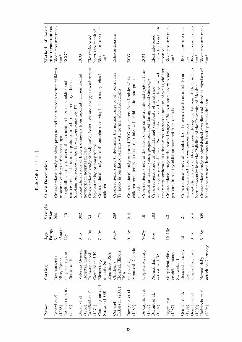
Tab

leC

.6:

(con

tinu

ed)

Pap

erSet

ting

Age

Ran

geSam

ple

Siz

eStu

dy

Des

crip

tion

Met

hod

ofhea

rtra

tem

easu

rem

ent

Ber

ard

etal

.(1

988)

Day

nurs

erie

s,N

ice,

Fran

ce6– 45

mth

s26

4C

ross

-sec

tion

alst

udy

ofbl

ood

pres

sure

and

hear

tra

tein

norm

alch

ildre

nm

easu

red

duri

ngro

utin

ech

eck-

ups

Blo

odpr

essu

rem

on-

itor

*B

erna

ards

etal

.(2

003)

unsp

ecifi

ed,th

eN

ethe

rlan

ds13

y41

0Lon

gitu

dina

lst

udy

toas

sess

the

asso

ciat

ion

betw

een

smok

ing

and

card

iova

scul

arfit

ness

insu

bje

cts

recr

uite

dfr

omse

cond

ary

scho

ols.

Smok

ing

prev

alen

ceat

age

13w

asap

prox

imat

ely

1%

EC

G*

Bet

auet

al.

(198

0)V

eter

ans

Gen

eral

Hos

pita

l,Tai

wan

0–1y

302

Lon

gitu

dina

lst

udy

ofE

CG

para

met

ers

from

rand

omly

chos

enno

rmal

new

born

sin

hosp

ital

nurs

ery

EC

G

Bra

dfiel

det

al.

(197

1)P

rim

ary

scho

ol,

Cam

brid

ge,U

K7–

10y

54C

ross

-sec

tion

alst

udy

ofbo

dybu

ild,h

eart

rate

and

ener

gyex

pend

itur

eof

boys

atte

ndin

gpr

imar

ysc

hool

Ele

ctro

de-b

ased

hear

tra

tem

onit

or*

Com

pagn

one

and

Stra

yer

(199

9)E

lem

enta

rysc

hool

s,Sa

nFr

anci

sco,

USA

7–10

y17

4C

ross

-sec

tion

alst

udy

ofca

rdio

vasc

ular

reac

tivi

tyin

elem

enta

rysc

hool

child

ren

Blo

odpr

essu

rem

on-

itor

*

Cui

and

Rob

erso

n(2

006)

Chi

ldre

n’s

Hos

pita

l,Illin

ois,

USA

0–18

y28

9C

ross

-sec

tion

alst

udy

tode

term

ine

the

norm

alra

nge

ofle

ftve

ntri

cula

rTei

inde

xin

paed

iatr

icpa

tien

tsw

ith

norm

alec

hoca

rdio

gram

sE

choc

ardi

ogra

m

Dav

igno

net

al.

(198

0)un

spec

ified

,M

ontr

eal,

Can

ada

0–16

y21

41C

ross

-sec

tion

alst

udy

ofno

rmal

EC

Gpa

ram

eter

sfr

omhe

alth

yw

hite

child

ren

recr

uite

dfr

omob

stet

ric

clin

ic,w

ell-ch

ildcl

inic

s,an

dpu

blic

scho

ols

EC

G

De

Cap

rio

etal

.(1

981)

unsp

ecifi

ed,It

aly

5–25

y46

Cro

ss-s

ecti

onal

stud

yof

the

effec

tof

age

onhe

art

rate

and

syst

olic

tim

ein

terv

alin

heal

thy

youn

gpe

ople

recr

uite

ddu

ring

norm

alch

eck-

ups

EC

G

Dur

ant

etal

.(1

992)

Nor

mal

daily

acti

viti

es,U

SA3–

5y19

0C

ross

-sec

tion

alst

udy

ofre

liabi

lity

and

vari

abili

tyof

hear

tra

tem

onit

orin

gin

youn

gch

ildre

n.Par

tici

pant

sre

crui

ted

from

long

itud

inal

stud

yin

toca

rdio

vasc

ular

dise

ase

risk

fact

ors

infa

mili

esof

youn

gch

ildre

n

Ele

ctro

de-b

ased

tele

met

ryhe

art

rate

mon

itor

*E

gger

etal

.(1

987)

Out

pati

ent

clin

icor

child

’sho

me,

Swit

zerl

and

10–1

6y43

Cro

ss-s

ecti

onal

stud

yof

the

norm

alra

nge

of24

-hou

ram

bula

tory

bloo

dpr

essu

rein

heal

thy

child

ren

recr

uite

dfr

omsc

hool

sB

lood

pres

sure

mon

-it

or*

Gem

elli

etal

.(1

989)

Hos

pita

lnu

rser

y,It

aly

4d21

Cro

ss-s

ecti

onal

stud

yof

circ

adia

nbl

ood

pres

sure

patt

erns

infu

ll-te

rmin

fant

sde

liver

edaf

ter

spon

tane

ous

labo

urB

lood

pres

sure

mon

-it

orG

emel

liet

al.

(199

0)un

spec

ified

,It

aly

0–1y

514

Lon

gitu

dina

lst

udy

ofbl

ood

pres

sure

duri

ngth

e1s

tye

arof

life

inin

fant

sbo

rnco

nsec

utiv

ely

atth

ePol

iclin

icof

the

Uni

vers

ity

ofM

essi

naB

lood

pres

sure

mon

-it

or*

Had

tste

inet

al.

(200

4)N

orm

alda

ilyac

tivi

ties

,Ger

man

y5–

18y

938

Cro

ss-s

ecti

onal

stud

yof

phys

iolo

gica

lci

rcad

ian

and

ultr

adia

nrh

ythm

sof

bloo

dpr

essu

rean

dhe

art

rate

inhe

alth

ysc

hool

child

ren

Blo

odpr

essu

rem

on-

itor

*

233

Tab

leC

.6:

(con

tinu

ed)

Pap

erSet

ting

Age

Ran

geSam

ple

Siz

eStu

dy

Des

crip

tion

Met

hod

ofhea

rtra

tem

easu

rem

ent

Har

shfie

ldet

al.

(199

4)N

orm

alda

ilyac

tivi

ties

,U

SA10

–18y

300

Cro

ss-s

ecti

onal

stud

yof

ambu

lato

rybl

ood

pres

sure

mon

itor

ing

inhe

alth

y,no

rmot

ensi

vech

ildre

nre

crui

ted

byad

vert

isem

ent

for

ast

udy

onca

rdio

vasc

ular

risk

fact

ors

inyo

uth

Blo

odpr

essu

rem

on-

itor

*

Hed

iger

etal

.(1

984)

unsp

ecifi

ed,

Phi

lade

lphi

a,U

SA12

–17y

621

Lon

gitu

dina

lst

udy

ofbl

ood

pres

sure

inbl

ack

adol

esce

nts,

recr

uite

dfr

oma

larg

ebi

rth

coho

rtst

udy

Man

ual

(rad

ial

pal-

pati

on)*

Iliff

and

Lee

(195

2)R

esea

rch

labo

rato

ry,U

SA0–

18y

197

Lon

gitu

dina

lst

udy

ofhe

art

rate

,re

spir

ator

yra

tean

dbo

dyte

mpe

ratu

rein

norm

alch

ildre

nM

anua

l(p

alpa

tion

orau

scul

tati

on)

Kah

net

al.

(199

3)Pae

diat

ric

Slee

pC

linic

,U

nive

rsity

Chi

ldre

n’s

Hos

pita

l,B

russ

els,

Bel

gium

3mth

s68

Cro

ss-s

ecti

onal

stud

yof

the

rela

tion

ship

betw

een

body

posi

tion

and

slee

pch

arac

teri

stic

sin

heal

thy

subje

cts

refe

rred

topa

edia

tric

slee

pcl

inic

follo

win

gst

udie

sco

nfirm

ing

norm

alsl

eep

beha

viou

r,an

dw

ith

nohi

stor

yof

slee

ppr

oble

ms

orap

noea

EC

Gˆ

Kru

llet

al.

(199

3)N

orm

alda

ilyac

tivi

ties

,Ger

man

y6–

10y

105

Cro

ss-s

ecti

onal

stud

yof

24-h

our

ambu

lato

rybl

ood

pres

sure

mon

itor

ing

inhe

alth

ych

ildre

nre

crui

ted

from

asc

hool

Blo

odpr

essu

rem

on-

itor

*Lin

dner

etal

.(1

985)

unsp

ecifi

ed,

Ger

man

y0–

4wks

30Lon

gitu

dina

lst

udy

tode

term

ine

the

influ

ence

ofhe

art

rate

onsy

stol

icti

me

inte

rval

sin

heal

thy

term

neon

ates

EC

Gan

dec

hoca

r-di

ogra

mLog

anet

al.

(200

0)D

ayti

me

mon

itor

ing

duri

ngno

rmal

daily

acti

viti

es,Sc

otla

nd

3–4y

20C

ross

-sec

tion

alst

udy

ofap

pare

ntle

vels

ofph

ysic

alac

tivi

tyin

youn

ghe

alth

ych

ildre

nTel

emet

ryhe

art

rate

mon

itor

*

Mac

farl

ane

etal

.(1

994)

Gen

eral

and

child

ren’

sho

spit

al,

post

nata

lcl

inic

s,pr

esch

ools

and

scho

ols,

Gla

sgow

,Sc

otla

nd

0–18

y17

82C

ross

-sec

tion

alst

udy

ofE

CG

para

met

ers

inhe

alth

y,no

rmal

lyde

velo

ped

child

ren,

and

child

ren

hosp

ital

ised

for

prob

lem

sth

atdi

dno

taff

ect

the

card

iova

scul

arsy

stem

EC

G

Mak

anet

al.

(200

5)un

spec

ified

,U

K14

–18y

250

Cas

e-co

ntro

lst

udy

ofle

ftve

ntri

cula

rvo

lum

ein

trai

ned

adol

esce

ntat

hlet

es(o

nly

data

from

cont

rolgr

oup

ofhe

alth

yad

oles

cent

sre

crui

ted

from

larg

ese

cond

ary

educ

atio

nbo

ardi

ngsc

hool

sin

clud

edin

revi

ew)

Ech

ocar

diog

ram

*

Mas

onet

al.

(200

7)un

spec

ified

,w

orld

wid

e10

–19y

1345

Cro

ss-s

ecti

onal

stud

yof

EC

Gpa

ram

eter

sin

norm

alhe

alth

yvo

lunt

eers

scre

ened

for

enro

lmen

tin

phar

mac

euti

calco

mpa

ny-s

pons

ored

clin

ical

tria

ls

EC

G

234

Tab

leC

.6:

(con

tinu

ed)

Pap

erSet

ting

Age

Ran

geSam

ple

Siz

eStu

dy

Des

crip

tion

Met

hod

ofhea

rtra

tem

easu

rem

ent

Mas

sin

etal

.(2

005)

Nor

mal

daily

acti

viti

es,B

elgi

um0–

16y

264

Cas

e-co

ntro

lst

udy

ofca

rdia

cra

tean

drh

ythm

patt

erns

inam

bula

tory

and

hosp

ital

ised

pati

ents

(onl

yda

tafr

omco

ntro

lgr

oup

ofhe

alth

yam

bula

tory

child

ren

incl

uded

inre

view

)

EC

G

Mim

ura

and

Mae

da(1

989)

Pri

vate

kind

erga

rten

,Ja

pan

4–6y

1069

Cro

ss-s

ecti

onal

stud

yof

phys

ical

fitne

ssin

youn

gch

ildre

nre

crui

ted

from

aki

nder

gart

enPen

-osc

illog

raph

*

Mul

ler

etal

.(1

989)

Med

ical

cent

res,

Fran

ce4–

18y

1014

14C

ross

-sec

tion

alst

udy

ofE

CG

para

met

ers

inch

ildre

nE

CG

*

Nib

oshi

etal

.(2

006)

unsp

ecifi

ed,Ja

pan

9–18

y97

0C

ross

-sec

tion

alst

udy

ofbr

achi

al-a

nkle

puls

ew

ave

velo

city

inhe

alth

yJa

pane

sech

ildre

nre

crui

ted

from

scho

olor

afte

rdo

ctor

’sco

nsul

tati

ons

for

func

tion

alm

urm

ur(p

atie

nts

and

heal

thy

sibl

ings

)

EC

G*

Obe

rlan

der

etal

.(1

999)

Bio

beha

viou

ral

Res

earc

hU

nit,

Cen

tre

for

Com

mun

ity

Chi

ldH

ealt

hR

esea

rch,

Van

couv

er,C

anad

a

4–8m

ths

24Lon

gitu

dina

lst

udy

ofca

rdia

cau

tono

mic

resp

onse

sto

acut

eno

xiou

sev

ents

inhe

alth

yin

fant

sre

crui

ted

atbi

rth

EC

G*

Pal

atin

iet

al.

(198

7)N

orm

alda

ilyac

tivi

ties

,It

aly

10–1

4y30

Cas

e-co

ntro

lst

udy

ofth

eeff

ect

ofen

dura

nce

trai

ning

onQ

-Tin

terv

alan

dca

rdia

cel

ectr

ical

stab

ility

(onl

yda

tafr

omco

ntro

lgr

oup

ofhe

alth

yno

rmot

ensi

vebo

ysra

ndom

lyse

lect

edfr

omsc

hool

incl

uded

inre

view

)

EC

G

Par

kan

dLee

(198

9)M

edic

alC

ente

rH

ospi

tal,

San

Ant

onio

,U

SA

5–14

9h21

9C

ross

-sec

tion

alst

udy

ofar

man

dca

lfbl

ood

pres

sure

inhe

alth

yfu

ll-te

rmin

fant

sre

crui

ted

atbi

rth

Blo

odpr

essu

rem

on-

itor

Par

kan

dM

enar

d(1

989)

Pae

diat

rici

ans’

office

san

dw

ell-ba

bycl

inic

s,Sa

nA

nton

io,U

SA

0–5y

1554

Cro

ss-s

ecti

onal

stud

yof

osci

llom

etri

cbl

ood

pres

sure

inpa

tien

tsan

dac

com

pany

ing

sibl

ings

atte

ndin

gpa

edia

tric

ians

’offi

ces

orw

ell-ba

bycl

inic

s,w

how

ere

com

plet

ely

heal

thy

orha

don

lym

inor

com

plai

nts

wit

hout

feve

r

Blo

odpr

essu

rem

on-

itor

Pei

rano

etal

.(1

988)

Chi

ld’s

hom

e,Fr

ance

5–24

wks

28C

ase-

cont

rolst

udy

ofni

ght

slee

phe

art

rate

patt

erns

inin

fant

sat

risk

for

SID

S(o

nly

data

from

cont

rolgr

oup

ofcl

inic

ally

and

neur

olog

ical

lyno

rmal

infa

nts

incl

uded

inre

view

)

EC

Gˆ

Per

eira

etal

.(1

984)

Hom

evi

sits

,P

hila

delp

hia,

USA

18–

19m

ths

21C

ross

-sec

tion

alst

udy

ofth

ere

lati

onsh

ipbe

twee

nhe

art

rate

,act

ivity,

and

ener

gyex

pend

itur

ein

heal

thy

mal

ein

fant

sre

crui

ted

from

ala

rge

long

itud

inal

stud

y

EC

G*

235

Tab

leC

.6:

(con

tinu

ed)

Pap

erSet

ting

Age

Ran

geSam

ple

Siz

eStu

dy

Des

crip

tion

Met

hod

ofhea

rtra

tem

easu

rem

ent

Piv

ikan

dD

ykm

an(2

004)

Res

earc

hla

bora

tory

,U

SA8–

10y

39C

ase-

cont

rolst

udy

ofth

eca

rdio

vasc

ular

resp

onse

tom

orni

ngnu

trit

ion

(onl

yda

tafr

omno

n-fa

stin

ggr

oup

ofhe

alth

ych

ildre

nre

crui

ted

from

loca

lco

mm

unity

incl

uded

inre

view

)

EC

G*

Poe

tset

al.

(199

1)C

hild

’sho

me,

UK

0–2y

42Lon

gitu

dina

lst

udy

ofbr

eath

ing

patt

erns

and

hear

tra

tein

full-

term

,he

alth

yin

fant

sse

lect

edat

rand

omE

CG

Rab

bia

etal

.(2

002)

Scho

ols,

Tur

in,

Ital

y12

–18y

2230

Cro

ss-s

ecti

onal

stud

yof

rest

ing

hear

tra

tein

rand

omly

sele

cted

child

ren

recr

uite

dfr

omsc

hool

sM

anua

l(r

adia

lpa

l-pa

tion

)*R

egec

ova

and

Kel

lero

va(1

995)

Kin

derg

arte

ns,

Bra

tisl

ava,

Slov

akR

epub

lic

3–7y

1542

Cro

ss-s

ecti

onal

stud

yof

the

asso

ciat

ion

betw

een

urba

ntr

affic

nois

ean

dbl

ood

pres

sure

inhe

alth

ych

ildre

nre

crui

ted

from

kind

erga

rten

sM

anua

l(r

adia

lpa

l-pa

tion

)*

Rek

awek

etal

.(2

003)

Nor

mal

daily

acti

viti

es,Pol

and

4–18

y37

2C

ross

-sec

tion

alst

udy

ofhe

art

rate

vari

abili

tyin

dice

sin

heal

thy

child

ren

EC

G

Rijn

beek

etal

.(2

001)

unsp

ecifi

ed,

Rot

terd

am,th

eN

ethe

rlan

ds

0–16

y19

12C

ross

-sec

tion

alst

udy

ofno

rmal

EC

Gpa

ram

eter

sin

heal

thy

child

ren

recr

uite

dfr

omch

ildhe

alth

cent

res,

prim

ary

and

seco

ndar

ysc

hool

sE

CG

Rob

erso

nan

dC

ui(2

007)

Chi

ldre

n’s

Hos

pita

l,Illin

ois,

USA

0–18

y30

8C

ross

-sec

tion

alst

udy

ofri

ght

vent

ricu

lar

Tei

inde

xin

paed

iatr

icpa

tien

tsw

ith

norm

alec

hoca

rdio

gram

sE

choc

ardi

ogra

m

Rog

ache

vska

iaan

dE

vdok

imov

(199

9)

Seco

ndar

ysc

hool

,Si

ktiv

kar,

Rus

sia

7–16

y72

6C

ross

-sec

tion

alst

udy

ofbl

ood

circ

ulat

ion

and

gas

exch

ange

inse

cond

ary

scho

olch

ildre

nM

anua

l(r

adia

lpa

l-pa

tion

)*

Rom

ano

etal

.(1

988)

Nor

mal

daily

acti

viti

es,It

aly

6–11

y32

Cro

ss-s

ecti

onal

stud

yof

EC

Gpa

ram

eter

sin

heal

thy

child

ren

recr

uite

das

volu

ntee

rsor

afte

rre

ques

ting

exam

inat

ion

prio

rto

unde

rtak

ing

spor

ting

acti

vity

EC

G

Sala

meh

etal

.(2

008)

Nor

mal

daily

acti

viti

es,

unsp

ecifi

edlo

cati

on

0–20

y61

6C

ross

-sec

tion

alst

udy

ofno

rmal

hear

tra

tein

heal

thy

child

ren

refe

rred

wit

hpa

lpit

atio

nsor

susp

ecte

dpa

roxy

smal

supr

aven

tric

ular

tach

ycar

dia,

inw

hom

afu

llcl

inic

alan

dec

hoca

rdio

grap

hic

exam

inat

ion

faile

dto

confi

rmth

esu

spec

ted

prob

lem

,an

ddi

dno

tfin

dan

yev

iden

ceof

stru

ctur

alca

rdia

cdi

seas

e,si

gnifi

cant

arrh

ythm

iaor

othe

rse

riou

sill

ness

EC

G

Sem

izel

etal

.(2

008)

unsp

ecifi

ed,B

ursa

,Tur

key

0–16

y22

41C

ross

-sec

tion

alst

udy

ofE

CG

para

met

ers

inhe

alth

ych

ildre

nre

crui

ted

from

nurs

ery,

prim

ary

and

seco

ndar

ysc

hool

s,ch

ildhe

alth

cent

res,

and

am

ater

nity

hosp

ital

EC

G

Sung

etal

.(2

008)

Scho

ols,

Hon

gK

ong

6–18

y14

842

Cro

ss-s

ecti

onal

stud

yof

bloo

dpr

essu

rein

Chi

nese

child

ren

recr

uite

dfr

ompr

imar

yan

dse

cond

ary

scho

ols

Blo

odpr

essu

rem

on-

itor

*

236

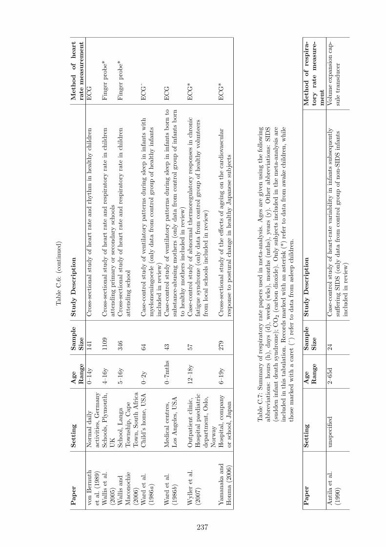
Tab

leC

.6:

(con

tinu

ed)

Pap

erSet

ting

Age

Ran

geSam

ple

Siz

eStu

dy

Des

crip

tion

Met

hod

ofhea

rtra

tem

easu

rem

ent

von

Ber

nuth

etal

.(1

989)

Nor

mal

daily

acti

viti

es,G

erm

any

0–14

y14

1C

ross

-sec

tion

alst

udy

ofhe

art

rate

and

rhyt

hmin

heal

thy

child

ren

EC

G

Wal

liset

al.

(200

5)Sc

hool

s,P

lym

outh

,U

K4–

16y

1109

Cro

ss-s

ecti

onal

stud

yof

hear

tra

tean

dre

spir

ator

yra

tein

child

ren

atte

ndin

gpr

imar

yor

seco

ndar

ysc

hool

sFin

ger

prob

e*

Wal

lisan

dM

acon

ochi

e(2

006)

Scho

ol,Lan

gaTow

nshi

p,C

ape

Tow

n,So

uth

Afr

ica

5–16

y34

6C

ross

-sec

tion

alst

udy

ofhe

art

rate

and

resp

irat

ory

rate

inch

ildre

nat

tend

ing

scho

olFin

ger

prob

e*

War

det

al.

(198

6a)

Chi

ld’s

hom

e,U

SA0–

2y64

Cas

e-co

ntro

lst

udy

ofve

ntila

tory

patt

erns

duri

ngsl

eep

inin

fant

sw

ith

mye

lom

enin

goce

le(o

nly

data

from

cont

rolgr

oup

ofhe

alth

yin

fant

sin

clud

edin

revi

ew)

EC

Gˆ

War

det

al.

(198

6b)

Med

ical

cent

res,

Los

Ang

eles

,U

SA0–

7mth

s43

Cas

e-co

ntro

lst

udy

ofve

ntila

tory

patt

erns

duri

ngsl

eep

inin

fant

sbo

rnto

subs

tanc

e-ab

usin

gm

othe

rs(o

nly

data

from

cont

rolgr

oup

ofin

fant

sbo

rnto

heal

thy

mot

hers

incl

uded

inre

view

)

EC

G

Wyl

ler

etal

.(2

007)

Out

pati

ent

clin

ic,

Hos

pita

lpa

edia

tric

depa

rtm

ent,

Osl

o,N

orw

ay

12–1

8y57

Cas

e-co

ntro

lst

udy

ofab

norm

alth

erm

oreg

ulat

ory

resp

onse

sin

chro

nic

fati

gue

synd

rom

e(o

nly

data

from

cont

rolgr

oup

ofhe

alth

yvo

lunt

eers

from

loca

lsc

hool

sin

clud

edin

revi

ew)

EC

G*

Yam

anak

aan

dH

onm

a(2

006)

Hos

pita

l,co

mpa

nyor

scho

ol,Ja

pan

6–19

y27

9C

ross

-sec

tion

alst

udy

ofth

eeff

ects

ofag

eing

onth

eca

rdio

vasc

ular

resp

onse

topo

stur

alch

ange

inhe

alth

yJa

pane

sesu

bje

cts

EC

G*

Tab

leC

.7:

Sum

mar

yof

resp

irat

ory

rate

pape

rsus

edin

met

a-an

alys

is.

Age

sar

egi

ven

usin

gth

efo

llow

ing

abbr

evia

tion

s:ho

urs

(h),

days

(d),

wee

ks(w

ks),

mon

ths

(mth

s),ye

ars

(y).

Oth

erab

brev

iati

ons:

SID

S(s

udde

nin

fant

deat

hsy

ndro

me)

;CO

2(c

arbo

ndi

oxid

e).

Onl

ysu

bje

cts

incl

uded

inth

em

eta-

anal

ysis

are

incl

uded

inth

ista

bula

tion

.R

ecor

dsm

arke

dw

ith

anas

teri

sk(*

)re

fer

toda

tafr

omaw

ake

child

ren,

whi

leth

ose

mar

ked

wit

ha

care

t(ˆ

)re

fer

toda

tafr

omas

leep

child

ren.

Pap

erSet

ting

Age

Ran

geSam

ple

Siz

eStu

dy

Des

crip

tion

Met

hod

ofre

spir

a-to

ryra

tem

easu

re-

men

tA

ntila

etal

.(1

990)

unsp

ecifi

ed2–

65d

24C

ase-

cont

rolst

udy

ofhe

art-

rate

vari

abili

tyin

infa

nts

subs

eque

ntly

suffe

ring

SID

S(o

nly

data

from

cont

rolgr

oup

ofno

n-SI

DS

infa

nts

incl

uded

inre

view

)

Vol

ume

expa

nsio

nca

p-su

letr

ansd

ucer

237

Tab

leC

.7:

(con

tinu

ed)

Pap

erSet

ting

Age

Ran

geSam

ple

Siz

eStu

dy

Des

crip

tion

Met

hod

ofre

spir

a-to

ryra

tem

easu

re-

men

tA

shto

nan

dC

onno

lly(1

971)

Res

earc

hla

bora

tory

,U

K44

–144

h22

Cro

ss-s

ecti

onal

stud

yof

hear

tra

tean

dre

spir

ator

yra

tedu

ring

cons

ecut

ive

slee

pcy

cles

inin

fant

sSt

rain

gaug

eˆ

Bal

asub

ram

ania

net

al.(2

006)

Chi

ldre

n’s

Hos

pita

l,C

henn

ai,

Indi

a

1mth

–5y

626

Cro

ss-s

ecti

onal

stud

yof

hear

tra

te,re

spir

ator

yra

te,an

dox

ygen

satu

rati

onin

heal

thy

child

ren

atte

ndin

gou

tpat

ient

sde

part

men

tfo

rim

mun

izat

ion

and/

orw

ell-ba

bych

eck-

ups

aspa

tien

tsor

sibl

ings

,or

post

edfo

rel

ecti

vesu

rger

y

Man

ual(o

bser

vati

on)*

Bha

ndar

iet

al.

(199

8)H

ospi

tal,

Cha

ndig

arh,

Indi

a1–

8wks

50Lon

gitu

dina

lst

udy

ofre

spir

ator

yra

teof

heal

thy

infa

nts

recr

uite

dat

birt

h(o

nly

data

from

norm

albi

rthw

eigh

tin

fant

sin

clud

edin

revi

ew)

Man

ual

(obs

erva

tion

orau

scul

tati

on)

Cur

zi-D

asca

lova

etal

.(1

981)

Hos

pita

l,Par

is,

Fran

ce0–

18w

ks57

Cro

ss-s

ecti

onal

stud

yof

resp

irat

ory

rate

inno

rmal

,fu

ll-te

rmin

fant

sre

crui

ted

from

hosp

ital

nurs

erie

sSt

rain

gaug

esˆ

Cur

zi-D

asca

lova

etal

.(1

983)

Hos

pita

l,Par

is,

Fran

ce2d

–18

wks

38C

ase-

cont

rolst

udy

ofre

spir

ator

yra

tedu

ring

slee

pin

sibl

ings

ofSI

DS

vict

ims

(onl

yda

tafr

omco

ntro

lgr

oup

ofno

rmal

infa

nts

wit

hno

fam

ilial

hist

ory

ofSI

DS

incl

uded

inre

view

)

Stra

inga

ugeˆ

Hop

penb

rouw

ers

etal

.(1

979)

Slee

pla

bora

tory

,U

SA1–

6mth

s25

Lon

gitu

dina

lst

udy

ofci

rcad

ian

patt

erns

inth

ere

spir

ator

yra

tein

neur

olog

ical

lyno

rmal

infa

nts

Exp

ired

CO

2m

onit

oran

dth

erm

isto

rH

oppe

nbro

uwer

set

al.(1

980)

Infa

ntsl

eep

labo

rato

ry,U

SA0–

6mth

s25

Lon

gitu

dina

lca

se-c

ontr

olst

udy

ofci

rcad

ian

patt

erns

inth

ere

spir

ator

yra

tein

sibl

ings

ofSI

DS

vict

ims

(onl

yda

tafr

omco

ntro

lgr

oup

ofno

n-SI

DS

infa

nts

incl

uded

inre

view

Exp

ired

CO

2m

onit

oran

dth

erm

isto

r

Iliff

and

Lee

(195

2)R

esea

rch

labo

rato

ry,U

SA0–

18y

197

Lon

gitu

dina

lst

udy

ofhe

art

rate

,re

spir

ator

yra

tean

dbo

dyte

mpe

ratu

rein

norm

alch

ildre

nM

anua

l(o

bser

vati

on)

Kah

net

al.

(199

3)Pae

diat

ric

Slee

pC

linic

,U

nive

rsity

Chi

ldre

n’s

Hos

pita

l,B

russ

els,

Bel

gium

3mth

s68

Cro

ss-s

ecti

onal

stud

yof

the

rela

tion

ship

betw

een

body

posi

tion

and

slee

pch

arac

teri

stic

sin

heal

thy

subje

cts

refe

rred

topa

edia

tric

slee

pcl

inic

follo

win

gst

udie

sco

nfirm

ing

norm

alsl

eep

beha

viou

r,an

dw

ith

nohi

stor

yof

slee

ppr

oble

ms

orap

noea

Stra

inga

uges

and

ther

-m

isto

rˆ

Mon

tgom

ery-

Dow

nsan

dT

hom

an(1

998)

Com

mun

ity

hosp

ital

and

child

’sho

me,

USA

0–6m

ths

88Lon

gitu

dina

lst

udy

ofqu

iet

slee

pre

spir

ator

yra

tes

infu

ll-te

rmno

rmal

infa

nts

recr

uite

ddu

ring

child

birt

hcl

asse

sC

apac

itiv

epr

essu

rese

nsit

ive

padˆ

Mor

ley

etal

.(1

990)

Chi

ld’s

hom

e,C

ambr

idge

,U

K0–

6mth

s29

8C

ross

-sec

tion

alst

udy

ofre

spir

ator

yra

tean

dse

veri

tyof

illne

ssin

child

ren

(onl

yda

tafr

omw

ellch

ildre

nre

crui

ted

rand

omly

from

the

birt

hre

gist

erin

clud

edin

revi

ew)

Man

ual

(obs

erva

tion

orau

scul

tati

on)

Nog

ues

etal

.(1

992)

Res

earc

hla

bora

tory

,Fr

ance

60–7

5d35

Cro

ss-s

ecti

onal

stud

yof

day-

tim

ean

dni

ght-

tim

ere

spir

ator

yra

tes

inno

rmal

infa

nts

Rub

ber

stra

psan

dth

erm

isto

rˆ

238

Tab

leC

.7:

(con

tinu

ed)

Pap

erSet

ting

Age

Ran

geSam

ple

Siz

eStu

dy

Des

crip

tion

Met

hod

ofre

spir

a-to

ryra

tem

easu

re-

men

tPoe

tset

al.

(199

1)C

hild

’sho

me,

UK

0–2y

42Lon

gitu

dina

lst

udy

ofbr

eath

ing

patt

erns

and

hear

tra

tein

full-

term

,he

alth

yin

fant

sse

lect

edat

rand

omP

ress

ure

caps

ule

onch

est

Ros

enth

alan

dB

ush

(200

0)un

spec

ified

,Lon

don,

UK

8–17

y10

6C

ross

-sec

tion

alst

udy

ofve

ntila

tory

vari

able

sin

heal

thy

child

ren

recr

uite

dfr

omsc

hool

sH

eliu

mdi

luti

onm

ixed

expi

red

gas

anal

ysis

*R

usco

niet

al.

(199

4)D

ayca

rece

ntre

sor

hosp

ital

s,It

aly

0–3y

618

Cro

ss-s

ecti

onal

stud

yof

resp

irat

ory

rate

inch

ildre

nre

crui

ted

from

day

care

cent

res

orho

spit

alin

pati

ent

orou

tpat

ient

depa

rtm

ents

,w

ith

noch

roni

cor

seve

reill

ness

,or

sign

sof

resp

irat

ory

infe

ctio

n

Man

ual

(aus

cult

a-ti

on)*

Wal

liset

al.

(200

5)Sc

hool

s,P

lym

outh

,U

K4–

16y

1109

Cro

ss-s

ecti

onal

stud

yof

hear

tra

tean

dre

spir

ator

yra

tein

child

ren

atte

ndin

gpr

imar

yor

seco

ndar

ysc

hool

sM

anua

l(o

bser

vati

on)*

Wal

lisan

dM

acon

ochi

e(2

006)

Scho

ol,Lan

gaTow

nshi

p,C

ape

Tow

n,So

uth

Afr

ica

5–16

y34

6C

ross

-sec

tion

alst

udy

ofhe

art

rate

and

resp

irat

ory

rate

inch

ildre

nat

tend

ing

scho

olM

anua

l(o

bser

vati

on)*

War

det

al.

(198

6a)

Chi

ld’s

hom

e,U

SA0–

2y64

Cas

e-co

ntro

lst

udy

ofve

ntila

tory

patt

erns

duri

ngsl

eep

inin

fant

sw

ith

mye

lom

enin

goce

le(o

nly

data

from

cont

rolgr

oup

ofhe

alth

yin

fant

sin

clud

edin

revi

ew)

Che

stw

alli

mpe

danc

eˆ

War

det

al.

(198

6b)

Med

ical

cent

res,

Los

Ang

eles

,U

SA0–

7mth

s43

Cas

e-co

ntro

lst

udy

ofve

ntila

tory

patt

erns

duri

ngsl

eep

inin

fant

sbo

rnto

subs

tanc

e-ab

usin

gm

othe

rs(o

nly

data

from

cont

rolgr

oup

ofin

fant

sbo

rnto

heal

thy

mot

hers

incl

uded

inre

view

)

Impe

danc

epn

eum

o-gr

am

239

Appendix D

Tables of normal heart rate and

respiratory rate

The following tables show selected points from the curves created in the meta-analysis

of heart rate and respiratory rate presented in Chapter 2. The ages in these tables were

chosen to ensure that the data presented here contains sufficient detail to reconstruct the

essential shapes of the curves. Thus, the data is more frequently sampled at younger ages,

where there is greatest variation in the heart rate and respiratory rate.

Table D.1: Mean, standard deviation, and selected centiles of heart rate from birth to 18 years, asdetermined by meta-analysis. Abbreviations used: years(y), months(m)

Age Mean Standard 1st 10th 25th 75th 90th 99thDeviation Centile Centile Centile Centile Centile Centile

0 127.12 15.927 90.081 107.05 116.44 137.92 147.53 164.181m 144.47 15.838 108.02 124.92 133.98 155.34 164.65 181.712m 143.52 15.78 107.17 123.79 133.12 154.41 163.85 180.593m 142.13 15.579 106.06 122.52 131.71 152.73 161.95 178.544m 140.55 15.41 104.69 121.08 130.08 150.87 159.88 176.395m 138.74 15.317 102.94 119.35 128.19 148.85 157.69 174.26m 136.74 15.266 100.94 117.39 126.11 146.71 155.41 171.977m 134.65 15.2 98.904 115.31 123.97 144.48 153.02 169.638m 132.55 15.083 97.001 113.23 121.88 142.22 150.58 167.189m 130.55 14.911 95.344 111.25 119.94 140.06 148.23 164.7210m 128.74 14.716 93.97 109.46 118.26 138.11 146.15 162.4411m 127.18 14.536 92.841 107.92 116.84 136.45 144.46 160.481y 125.87 14.413 91.839 106.61 115.65 135.09 143.17 158.91y 2m 123.66 14.404 89.659 104.38 113.48 132.91 141.35 156.671y 4m 121.48 14.578 87.023 102.3 111.18 130.85 139.7 154.851y 6m 119.29 14.584 84.756 100.42 108.97 128.64 137.7 152.611y 8m 117.19 14.447 82.961 98.673 106.98 126.47 135.55 150.181y 10m 115.21 14.347 81.201 96.907 105.09 124.44 133.53 147.952y 113.45 14.284 79.606 95.322 103.41 122.68 131.79 146.062y 2m 111.94 14.239 78.228 93.962 101.98 121.19 130.33 144.482y 4m 110.59 14.216 76.973 92.738 100.7 119.87 129.06 143.11

240

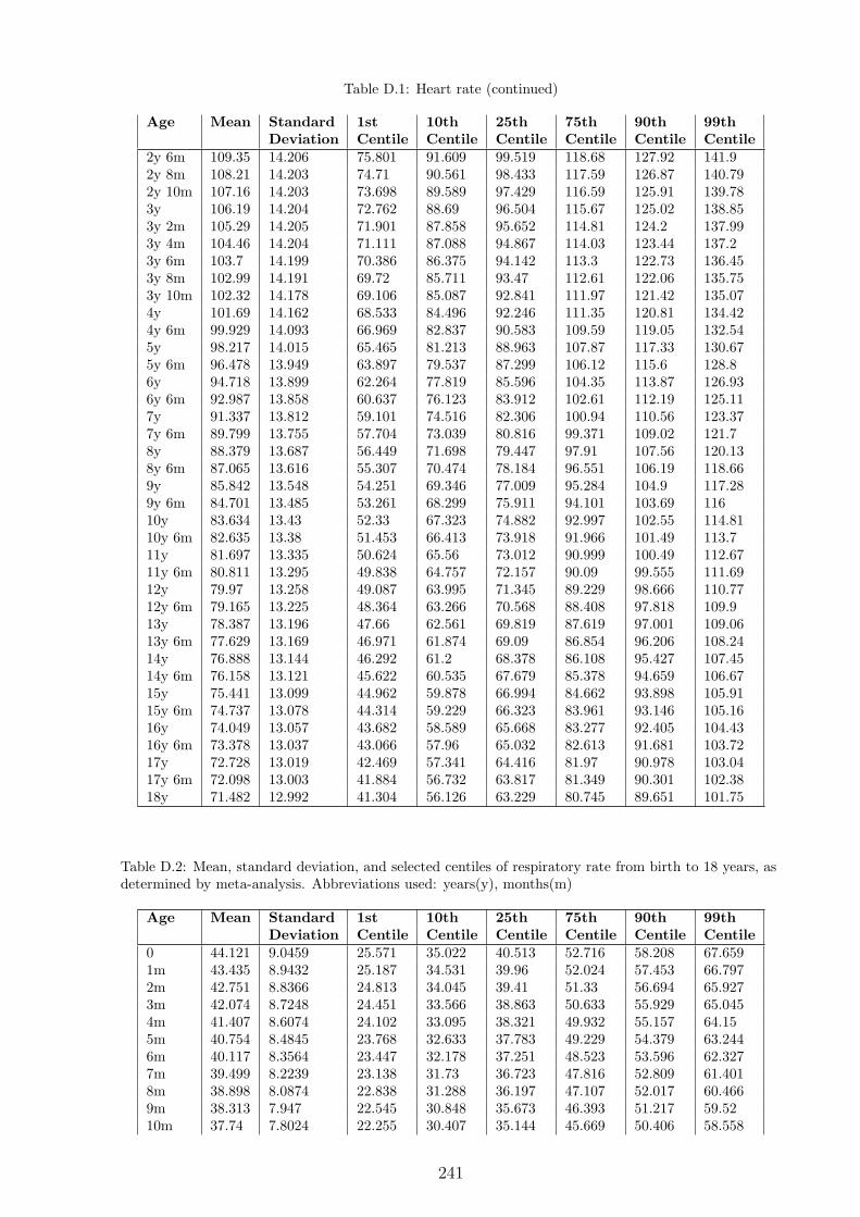
Table D.1: Heart rate (continued)

Age Mean Standard 1st 10th 25th 75th 90th 99thDeviation Centile Centile Centile Centile Centile Centile

2y 6m 109.35 14.206 75.801 91.609 99.519 118.68 127.92 141.92y 8m 108.21 14.203 74.71 90.561 98.433 117.59 126.87 140.792y 10m 107.16 14.203 73.698 89.589 97.429 116.59 125.91 139.783y 106.19 14.204 72.762 88.69 96.504 115.67 125.02 138.853y 2m 105.29 14.205 71.901 87.858 95.652 114.81 124.2 137.993y 4m 104.46 14.204 71.111 87.088 94.867 114.03 123.44 137.23y 6m 103.7 14.199 70.386 86.375 94.142 113.3 122.73 136.453y 8m 102.99 14.191 69.72 85.711 93.47 112.61 122.06 135.753y 10m 102.32 14.178 69.106 85.087 92.841 111.97 121.42 135.074y 101.69 14.162 68.533 84.496 92.246 111.35 120.81 134.424y 6m 99.929 14.093 66.969 82.837 90.583 109.59 119.05 132.545y 98.217 14.015 65.465 81.213 88.963 107.87 117.33 130.675y 6m 96.478 13.949 63.897 79.537 87.299 106.12 115.6 128.86y 94.718 13.899 62.264 77.819 85.596 104.35 113.87 126.936y 6m 92.987 13.858 60.637 76.123 83.912 102.61 112.19 125.117y 91.337 13.812 59.101 74.516 82.306 100.94 110.56 123.377y 6m 89.799 13.755 57.704 73.039 80.816 99.371 109.02 121.78y 88.379 13.687 56.449 71.698 79.447 97.91 107.56 120.138y 6m 87.065 13.616 55.307 70.474 78.184 96.551 106.19 118.669y 85.842 13.548 54.251 69.346 77.009 95.284 104.9 117.289y 6m 84.701 13.485 53.261 68.299 75.911 94.101 103.69 11610y 83.634 13.43 52.33 67.323 74.882 92.997 102.55 114.8110y 6m 82.635 13.38 51.453 66.413 73.918 91.966 101.49 113.711y 81.697 13.335 50.624 65.56 73.012 90.999 100.49 112.6711y 6m 80.811 13.295 49.838 64.757 72.157 90.09 99.555 111.6912y 79.97 13.258 49.087 63.995 71.345 89.229 98.666 110.7712y 6m 79.165 13.225 48.364 63.266 70.568 88.408 97.818 109.913y 78.387 13.196 47.66 62.561 69.819 87.619 97.001 109.0613y 6m 77.629 13.169 46.971 61.874 69.09 86.854 96.206 108.2414y 76.888 13.144 46.292 61.2 68.378 86.108 95.427 107.4514y 6m 76.158 13.121 45.622 60.535 67.679 85.378 94.659 106.6715y 75.441 13.099 44.962 59.878 66.994 84.662 93.898 105.9115y 6m 74.737 13.078 44.314 59.229 66.323 83.961 93.146 105.1616y 74.049 13.057 43.682 58.589 65.668 83.277 92.405 104.4316y 6m 73.378 13.037 43.066 57.96 65.032 82.613 91.681 103.7217y 72.728 13.019 42.469 57.341 64.416 81.97 90.978 103.0417y 6m 72.098 13.003 41.884 56.732 63.817 81.349 90.301 102.3818y 71.482 12.992 41.304 56.126 63.229 80.745 89.651 101.75

Table D.2: Mean, standard deviation, and selected centiles of respiratory rate from birth to 18 years, asdetermined by meta-analysis. Abbreviations used: years(y), months(m)

Age Mean Standard 1st 10th 25th 75th 90th 99thDeviation Centile Centile Centile Centile Centile Centile

0 44.121 9.0459 25.571 35.022 40.513 52.716 58.208 67.6591m 43.435 8.9432 25.187 34.531 39.96 52.024 57.453 66.7972m 42.751 8.8366 24.813 34.045 39.41 51.33 56.694 65.9273m 42.074 8.7248 24.451 33.566 38.863 50.633 55.929 65.0454m 41.407 8.6074 24.102 33.095 38.321 49.932 55.157 64.155m 40.754 8.4845 23.768 32.633 37.783 49.229 54.379 63.2446m 40.117 8.3564 23.447 32.178 37.251 48.523 53.596 62.3277m 39.499 8.2239 23.138 31.73 36.723 47.816 52.809 61.4018m 38.898 8.0874 22.838 31.288 36.197 47.107 52.017 60.4669m 38.313 7.947 22.545 30.848 35.673 46.393 51.217 59.5210m 37.74 7.8024 22.255 30.407 35.144 45.669 50.406 58.558

241

Table D.2: Respiratory rate (continued)

Age Mean Standard 1st 10th 25th 75th 90th 99thDeviation Centile Centile Centile Centile Centile Centile

11m 37.174 7.6527 21.965 29.961 34.606 44.93 49.575 57.5711y 36.611 7.4966 21.671 29.503 34.054 44.167 48.718 56.551y 2m 35.468 7.1592 21.061 28.541 32.887 42.545 46.891 54.3711y 4m 34.282 6.783 20.421 27.508 31.626 40.776 44.894 51.9811y 6m 33.065 6.3767 19.772 26.434 30.305 38.907 42.778 49.4411y 8m 31.87 5.9652 19.154 25.387 29.008 37.055 40.676 46.9081y 10m 30.759 5.5769 18.607 24.433 27.819 35.342 38.728 44.5542y 29.771 5.2303 18.151 23.616 26.791 33.847 37.022 42.4862y 2m 28.916 4.93 17.794 22.945 25.938 32.588 35.581 40.7322y 4m 28.182 4.6707 17.53 22.41 25.245 31.546 34.381 39.2612y 6m 27.551 4.4426 17.347 21.989 24.686 30.679 33.375 38.0172y 8m 27.001 4.2364 17.231 21.657 24.229 29.944 32.515 36.9422y 10m 26.515 4.0457 17.164 21.391 23.848 29.305 31.761 35.9883y 26.079 3.8671 17.132 21.172 23.521 28.737 31.084 35.1253y 2m 25.684 3.6998 17.121 20.986 23.233 28.224 30.469 34.3353y 4m 25.326 3.544 17.121 20.824 22.975 27.756 29.907 33.613y 6m 24.999 3.4005 17.124 20.677 22.742 27.329 29.393 32.9463y 8m 24.7 3.2698 17.126 20.542 22.527 26.938 28.923 32.343y 10m 24.427 3.1522 17.122 20.416 22.329 26.581 28.495 31.7894y 24.175 3.0472 17.111 20.294 22.143 26.254 28.105 31.2884y 6m 23.515 2.7994 17.015 19.939 21.634 25.411 27.114 30.0395y 22.944 2.6327 16.821 19.571 21.16 24.711 26.319 29.075y 6m 22.425 2.5256 16.544 19.183 20.701 24.108 25.656 28.2956y 21.947 2.4599 16.216 18.786 20.259 23.577 25.091 27.6616y 6m 21.505 2.4181 15.871 18.398 19.843 23.105 24.596 27.1227y 21.098 2.3869 15.538 18.032 19.458 22.678 24.15 26.6437y 6m 20.722 2.3595 15.227 17.692 19.105 22.288 23.74 26.2058y 20.374 2.3361 14.935 17.376 18.778 21.93 23.363 25.8048y 6m 20.052 2.3204 14.651 17.075 18.473 21.603 23.022 25.4479y 19.757 2.3169 14.364 16.785 18.185 21.311 22.723 25.1449y 6m 19.489 2.3279 14.071 16.503 17.914 21.055 22.47 24.90210y 19.248 2.3521 13.774 16.232 17.661 20.833 22.261 24.71810y 6m 19.031 2.3845 13.483 15.974 17.425 20.642 22.086 24.57711y 18.833 2.4176 13.209 15.734 17.208 20.47 21.931 24.45711y 6m 18.645 2.4426 12.962 15.514 17.006 20.301 21.775 24.32712y 18.453 2.4524 12.748 15.311 16.812 20.12 21.596 24.15812y 6m 18.248 2.4452 12.559 15.114 16.614 19.913 21.382 23.93613y 18.019 2.4266 12.374 14.909 16.401 19.674 21.129 23.66413y 6m 17.765 2.407 12.166 14.681 16.162 19.409 20.85 23.36514y 17.49 2.3959 11.916 14.419 15.895 19.127 20.56 23.06414y 6m 17.201 2.3966 11.626 14.13 15.605 18.838 20.272 22.77615y 16.907 2.4047 11.313 13.825 15.304 18.547 19.989 22.50115y 6m 16.616 2.4116 11.006 13.526 15.004 18.257 19.707 22.22616y 16.336 2.4082 10.734 13.25 14.721 17.97 19.422 21.93916y 6m 16.073 2.3896 10.514 13.01 14.465 17.688 19.135 21.63217y 15.829 2.3552 10.35 12.811 14.24 17.417 18.848 21.30817y 6m 15.603 2.3066 10.237 12.647 14.043 17.154 18.559 20.96918y 15.38 2.24 10.168 12.509 13.862 16.884 18.25 20.591

242