South  Texas  Project  Risk-­‐Informed  GSI-­‐191  Evaluation    

 

Means of Aggregation and NUREG-1829: Geometric and Arithmetic Means

       

                     Document:  STP-­‐RIGSI191-­‐ARAI.01  Revision:  1  Date:  June  13,  2013    Prepared  by:    David  Morton,  The  University  of  Texas  at  Austin  Ying-­‐An  Pan,  The  University  of  Texas  at  Austin  Jeremy  Tejada,  The  University  of  Texas  at  Austin    Pending  Review  by:    Ernie  J.  Kee,  South  Texas  Project  Zahra  Mohaghegh,  University  of  Illinois  at  Urbana-­‐Champaign  Seyed  A.  Reihani,  Soteria  Consultants    

Means of Aggregation and NUREG-1829:Geometric and Arithmetic Means

David Morton, Ying-An Pan, and Jeremy TejadaThe University of Texas at Austin

June 13, 2013

Abstract

We review methods of combining the probability distributions elicited from multiple experts toobtain a single probability distribution. More specifically, we describe the relative merits of thearithmetic mean (AM) and geometric mean (GM) as ways of performing this aggregation in thecontext of probabilities associated with rare events. We focus on a study known as NUREG-1829 [7], which includes an expert elicitation of quantiles governing the (annual) frequency of aloss-of-coolant accident (LOCA) in BWRs and PWRs. Examining a set of PWR results fromNUREG-1829, we conclude that the GM represents a consistently sensible notion of the middleof the opinions expressed by nine experts. We further conclude that the AM is inappropriatefor representing the center of the group’s opinion for large effective break sizes. Instead, as thebreak size grows large a single expert’s opinion dominates the combination produced by theAM.

1 Introduction

We discuss the arithmetic mean (AM) and geometric mean (GM) as techniques to aggregate prob-

ability distributions elicited from multiple experts into a single distribution that represents some

notion of group consensus. We specifically study the results obtained by combining the quantiles

elicited from experts in Tregoning et al. [7], known as NUREG-1829. This expert elicitation in-

volves quantiles (5th, 50th, and 95th percentiles) for exceedance frequencies for a loss-of-coolant

accident (LOCA) in BWRs and PWRs. In NUREG-1829, these quantiles are elicited for breaks

in the six effective break-size categories given in Table 1 for three time periods: current-day (25

years fleet average), end-of-plant-license (40 years fleet average), and end-of-plant-license-renewal

(60 years fleet average). We restrict attention to the PWR fleet, and to illustrate ideas, we restrict

attention to the results for the current-day time period.

2 Background

Suppose x1, x2, . . . , xn ∈ R+ represent n data points. There are multiple notions of what constitutes

the center of such a data set. The AM and GM represent the center, respectively, via:

AM =1n

n∑i=1

xi and (1a)

GM =

(n∏i=1

xi

)1/n

. (1b)

1

Table 1: NUREG-1829 LOCA categories for effective break sizes

Effective break size(inch) Category

12 category 1

158 category 2

3 category 37 category 414 category 531 category 6

The AM and GM satisfy the following inequality:(n∏i=1

xi

)1/n

≤ 1n

n∑i=1

xi, (2)

i.e., the GM’s value is at most that of the AM. Equality holds in (2) only if x1 = x2 = · · · = xn.

Because (n∏i=1

xi

)1/n

= 10

0B@ 1n

n∑i=1

log(xi)

1CA,

we can think of the GM as averaging the “exponents” of the data, x1, x2, . . . , xn, rather than directly

averaging the x-values. As we will see, if we most naturally visualize the data on a log-scale then

there is a strong argument for using the GM in place of the AM, particularly when the data exhibit

considerable variability.

We can assign different weights to each data point and generalize the summary measures of

equation (1) to:

n∑i=1

wixi and (3a)

n∏i=1

xwii , (3b)

where the weights wi ≥ 0, i = 1, . . . , n, satisfy∑n

i=1wi = 1. If each point is equally weighted, i.e.,

wi = 1/n, i = 1, . . . , n, then equations (3a) and (3b) reduce to (1a) and (1b), respectively. Other

widely used notions of the middle of a data set include the median, where the median is defined

as follows. Let x(1) ≤ x(2) ≤ · · · ≤ x(n) be the n data points reindexed so that they ascend. The

2

median defines the middle point by:

x(n+12

) or (4a)12

(x(n

2) + x(n

2+1)), (4b)

where we use (4a) if n is odd and (4b) if n is even.

One important application of the above ideas involves combining probability distributions of

multiple experts. Suppose n experts have given α-level quantiles, say, of a LOCA exceedance

frequency for a specific break size. If α = 0.5 then these are the median value of each expert’s

distribution. Denote the quantiles of the n experts by qα,1, qα,2, . . . , qα,n. Taking x1 = qα,1, x2 =

qα,2,. . . , xn = qα,n, we can apply one of the aggregation formulas from (1), (3), or (4) to determine

a single α-level quantile that summarizes the views of the experts.

If each expert has a full distribution, i.e., a quantile level for all α ∈ [0, 1], then we can apply an

aggregation rule, quantile-by-quantile, to construct a single probability distribution that represents

the views of the experts. The equally weighted and unequally weighted arithmetic and geometric

means provide a family of ways to combine the distributions of the individual experts.

There is a significant literature on combining expert opinion. See, for example, the discussions

in [2, 3, 4, 5] and references therein. It is not our purpose to survey such methods. Nor is it our

goal to argue definitively for one method being the universal “right choice.” In fact, impossibility

theorems—in the spirit of Arrow’s seminal work [1]—establish that no rule of aggregation can simul-

taneously satisfy certain sets of seemingly compelling properties; see the discussion in French [4].

Two such properties involve: (i) updating the distribution when new information is learned and (ii)

marginalizing the distribution by integrating out one component. Updating or marginalizing can

first be performed on the distributions of the individual experts, and then the results combined.

Or, the updating or marginalizing can be done on the aggregated, group distribution. The desirable

properties are that the results be consistent regardless of which way the updating is done. The GM

is consistent under (i) but not (ii) and the opposite result holds for the AM.

Our goal is more empirical in nature and tied to combining the type of rare-event probabilities

from multiple experts as investigated in NUREG-1829. Tregoning et al. [7] indicate that the results

of NUREG-1829 are sensitive to the method used to combine the individual expert estimates. Our

analysis in this report fully agrees that this is the case, particularly as we move from frequencies for

small breaks to those for large breaks; i.e., as the associated probabilities shrink and the disparity

among expert opinion grows. We do not make sweeping conclusions. Instead, in the context of

3

NUREG-1829, we conclude that the geometric mean represents the middle of the opinions expressed

by nine experts. And, we conclude that the arithmetic mean is inappropriate for representing the

center of the group’s opinion, particularly for large effective break sizes.

3 Aggregating Expert Opinion: NUREG-1829

In NUREG-1829, estimates from nine experts were elicited for PWRs for the 5th, 50th, and 95th

percentiles for frequencies of the break-size categories 1-6 (see Table 1). Here we focus on the

current-day (25 years fleet average) results. The expert elicitation includes piping and nonpiping

contributions with multiple subsystems for each. For piping contributions the subsystems include:

Reactor Coolant Piping: Hot Leg; Reactor Coolant Piping: Cold/Crossover Legs; Surge Line;

Safety Injection System: Accumulator Lines; Safety Injection System: Direct Volume Injection

Lines; Drain Lines; Chemical & Volume Control System; Residual Heat Removal System; Safety

Relief Valve Lines; Pressurizer Spray Lines; Reactor Head Lines; and, Instrumentation Lines. For

nonpiping contributions the subsystems include: Reactor Pressure Vessel; Pumps; Valves; Pressur-

izer; and, Steam Generator. Within each of the nonpiping subsystems, expert opinion was elicited

for a number of individual components. For example, for the Steam Generator subsystem, the indi-

vidual components are: Tube Rupture; Manway Bolts; Shell; Nozzles; and, Tube Sheet. We point

to the Steam Generator subsystem in particular because NUREG-1829 gives summary quantiles

for categories 1-6 both with, and without, contributions due to Stream Generator Tube Rupture

(SGTR) frequencies. That said, the summary quantiles only differ for categories 1 and 2; i.e., the

results with and without SGTR contributions are identical for categories 3-6. To date, STP’s pilot

effort in a risk-informed resolution of GSI-191 indicates that categories 1 and 2 do not contribute

to system failures, and hence the decision to include or exclude SGTR contributions in initiating

frequencies appears to have no effect on the analysis.

3.1 NUREG-1829: Category 1

NUREG-1829 employs an error-factor adjustment scheme that accounts for possible overconfidence

in the opinions of individual experts. We do not detail that scheme here, but roughly speaking,

for experts whose uncertainty ranges were relatively small, the error-factor adjustment scheme has

the effect of increasing their ranges; i.e., decreasing the 5th percentile and increasing the 95th

percentile. Figure 1 shows the 5th, 50th, and 95th percentiles for each of the nine experts after

the error-factor adjustment, repeating their labels from NUREG-1829: Experts A, B, C, E, G, H,

4

0"1"2"3"4"5"6"7"8"9"

10"11"12"

1.00E.06"

1.00E.05"

1.00E.04"

1.00E.03"

1.00E.02"

1.00E.01"

1.00E+00"

Expe

rt"or"G

roup

"Es9mate"

Frequency"

Category"1"Break"."Current"Day"Es9mates"AM"

GM"

Expert"A"

Expert"B"

Expert"C"

Expert"E"

Expert"G"

Expert"H"

Expert"I"

Expert"J"

Expert"L"

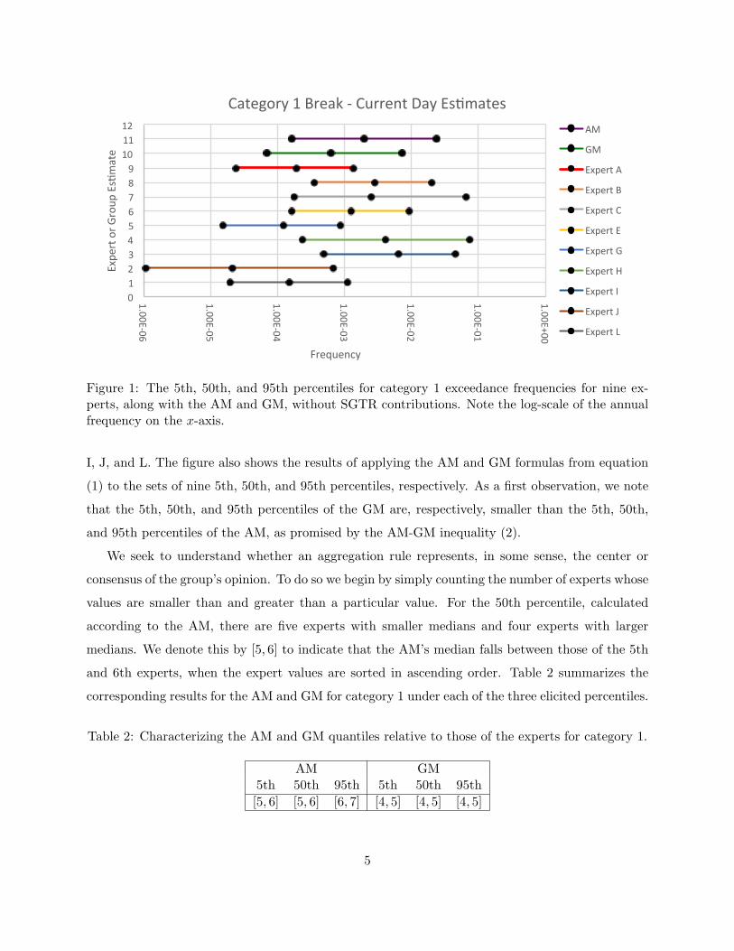
Figure 1: The 5th, 50th, and 95th percentiles for category 1 exceedance frequencies for nine ex-perts, along with the AM and GM, without SGTR contributions. Note the log-scale of the annualfrequency on the x-axis.

I, J, and L. The figure also shows the results of applying the AM and GM formulas from equation

(1) to the sets of nine 5th, 50th, and 95th percentiles, respectively. As a first observation, we note

that the 5th, 50th, and 95th percentiles of the GM are, respectively, smaller than the 5th, 50th,

and 95th percentiles of the AM, as promised by the AM-GM inequality (2).

We seek to understand whether an aggregation rule represents, in some sense, the center or

consensus of the group’s opinion. To do so we begin by simply counting the number of experts whose

values are smaller than and greater than a particular value. For the 50th percentile, calculated

according to the AM, there are five experts with smaller medians and four experts with larger

medians. We denote this by [5, 6] to indicate that the AM’s median falls between those of the 5th

and 6th experts, when the expert values are sorted in ascending order. Table 2 summarizes the

corresponding results for the AM and GM for category 1 under each of the three elicited percentiles.

Table 2: Characterizing the AM and GM quantiles relative to those of the experts for category 1.

AM GM5th 50th 95th 5th 50th 95th

[5, 6] [5, 6] [6, 7] [4, 5] [4, 5] [4, 5]

5

For each quantile we have nine experts and hence sorting the values, say, for the 50th percentile,

the 5th expert is in the middle (at least as measured by the median). The AM and GM values will

not (in general) exactly coincide with the value of any single expert. Hence, for the AM and GM

the notion of being in the center of the group’s opinion is best represented by a result that is either

[4, 5] or [5, 6]. In this sense, the results of Table 2 indicate that both the AM and GM represent the

center of the group’s opinions. (The 95th percentile for the AM is slightly larger, falling between

the 6th and 7th ascending values of the nine experts.)

We can also compare the AM and GM results by comparing their ratios. We know by the

AM-GM inequality (2) that the AM-to-GM ratio exceeds one. Table 3 shows these ratios for the

5th, 50th, and 95th percentiles for category 1.

Table 3: Ratio of AM-to-GM percentiles for category 1.

5th 50th 95th2 3 3

3.2 NUREG-1829: Categories 1-6

Examining category 1 in the previous section has allowed us to illustrate ideas. However for GSI-

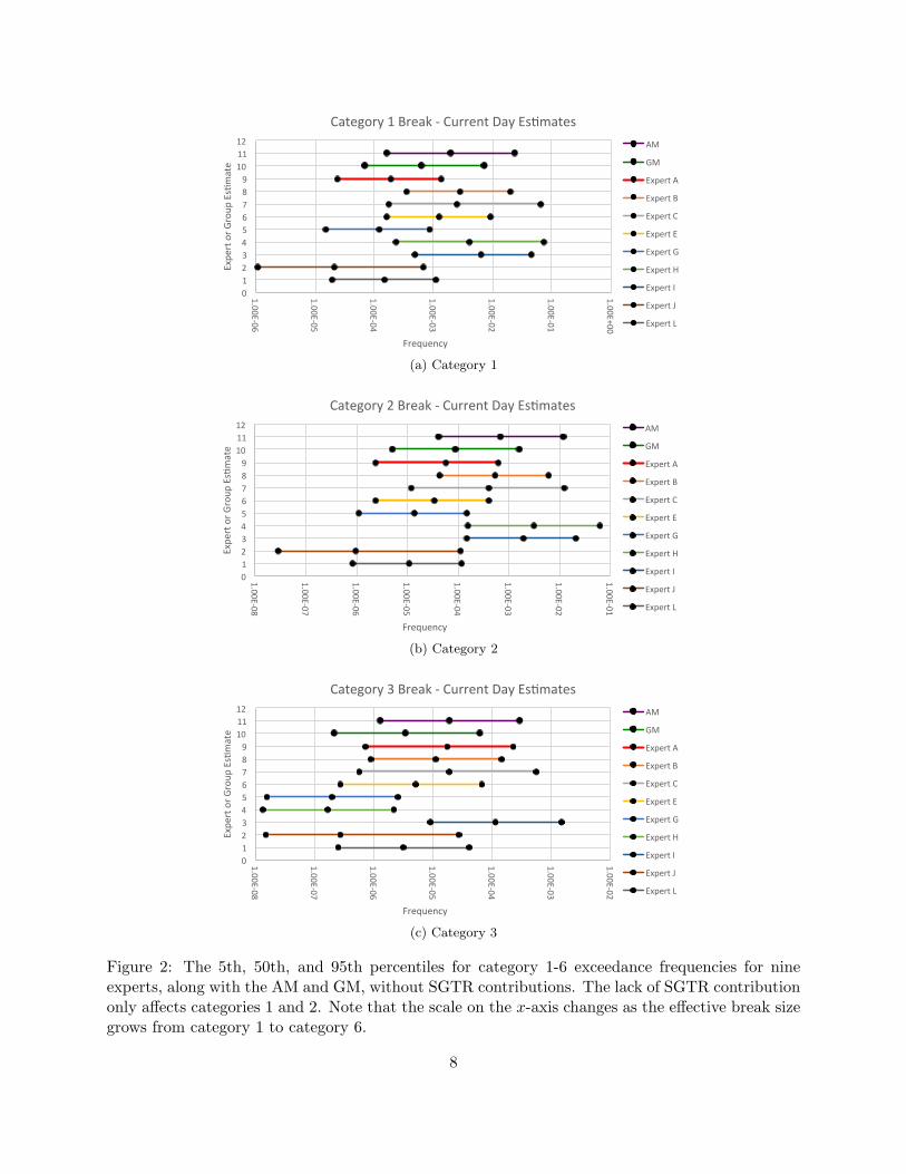
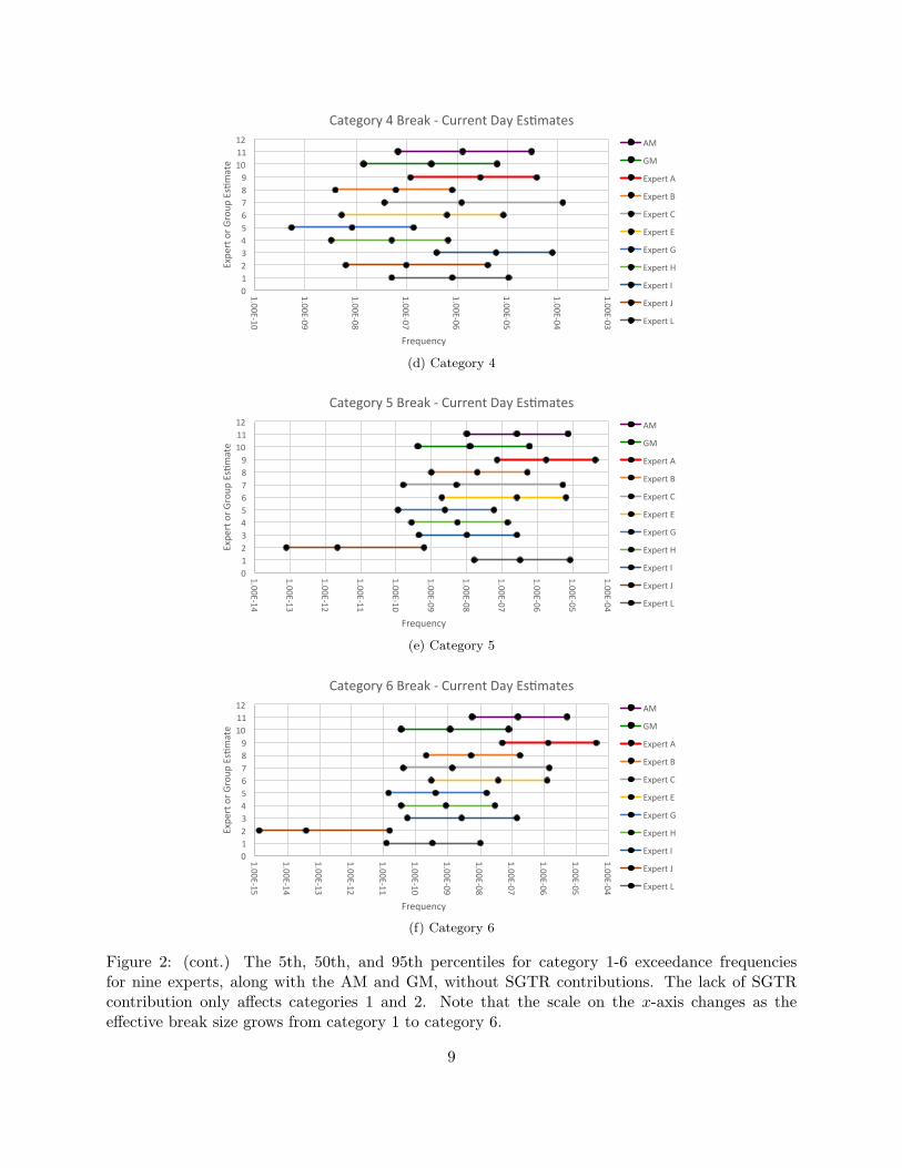
191, results for larger break sizes are of foremost interest. Figure 2 replicates Figure 1 in panel (a),

and includes the other five categories in panels (b)-(f). The plots again account for NUREG-1829’s

error-factor adjustment scheme. The six plots again capture the 5th, 50th, and 95th percentiles

of the nine experts along with the same percentiles for the AM and GM aggregation rules. When

examining differences and apparent similarities between the six graphs, we should be careful to

note that the log-scale plots of the annual frequencies on the x-axis differ from one plot to the next,

descending (very roughly) by an order of magnitude from one category to the next and tending to

increase in disparity as the break size grows.

Table 4 extends Table 2 to include the five larger break-size categories. Our observation that

the GM represents well the center of the group’s distributions for the case of category 1 extends

to the other five categories with all of the percentiles falling between the 4th and 5th, or 5th and

6th sorted values, out of nine experts, except for the 5th percentile for category 3. Even for this

one apparent aberration, we can see from Figure 2c that the numerical value of the 5th percentile

of the GM is relatively close to those of the fourth and fifth sorted 5th percentiles; i.e., the 5th

6

percentiles of Experts L and E.

The AM values in Table 4 tell a starkly different story. As the effective break size grows, the

quantiles of the AM aggregation scheme tend to become increasingly extreme. In category 6, each

of the quantiles of the AM are larger than those of eight of the nine experts, as indicated by [8, 9].

Focusing on category 6, the median of the AM is larger than the 95th percentile of five of the nine

experts, and the 5th percentile of the AM is larger than the median of seven of the nine experts.

As can be seen from Figure 2f, Expert A’s values are significantly larger than those of the rest of

the group. Expert A’s opinion dominates the combined opinion when using the AM for category 6,

and it is impossible to view the AM as reasonably representing the center of the group’s opinion.

Table 4: Characterizing the AM and GM quantiles relative to those of the experts for all categories.

AM GMCategory 5th 50th 95th 5th 50th 95th

Category 1 [5, 6] [5, 6] [6, 7] [4, 5] [4, 5] [4, 5]Category 2 [6, 7] [7, 8] [6, 7] [5, 6] [5, 6] [5, 6]Category 3 [8, 9] [8, 9] [7, 8] [3, 4] [4, 5] [4, 5]Category 4 [7, 8] [7, 8] [6, 7] [5, 6] [4, 5] [4, 5]Category 5 [7, 8] [7, 8] [7, 8] [4, 5] [5, 6] [5, 6]Category 6 [8, 9] [8, 9] [8, 9] [4, 5] [4, 5] [4, 5]

Table 5 extends Table 3 to include results for categories 2-6. We see that the relatively modest

ratio of the AM to the GM in category 1 grows large in categories 5 and 6, with the ratios of the

medians in category 6 exceeding two orders of magnitude.

Table 5: Ratio of AM-to-GM percentiles for categories 1-6.

Category 5th 50th 95thcategory 1 2 3 3category 2 8 8 7category 3 6 6 5category 4 5 4 5category 5 24 22 12category 6 169 125 64

7

0"1"2"3"4"5"6"7"8"9"

10"11"12"

1.00E.06"

1.00E.05"

1.00E.04"

1.00E.03"

1.00E.02"

1.00E.01"

1.00E+00"

Expe

rt"or"G

roup

"Es9mate"

Frequency"

Category"1"Break"."Current"Day"Es9mates"AM"

GM"

Expert"A"

Expert"B"

Expert"C"

Expert"E"

Expert"G"

Expert"H"

Expert"I"

Expert"J"

Expert"L"

(a) Category 1

0"1"2"3"4"5"6"7"8"9"

10"11"12"

1.00E.08"

1.00E.07"

1.00E.06"

1.00E.05"

1.00E.04"

1.00E.03"

1.00E.02"

1.00E.01"

Expe

rt"or"G

roup

"Es8mate"

Frequency"

Category"2"Break"."Current"Day"Es8mates"AM"

GM"

Expert"A"

Expert"B"

Expert"C"

Expert"E"

Expert"G"

Expert"H"

Expert"I"

Expert"J"

Expert"L"

(b) Category 2

0"1"2"3"4"5"6"7"8"9"

10"11"12"

1.00E.08"

1.00E.07"

1.00E.06"

1.00E.05"

1.00E.04"

1.00E.03"

1.00E.02"

Expe

rt"or"G

roup

"Es8mate"

Frequency"

Category"3"Break"."Current"Day"Es8mates"AM"

GM"

Expert"A"

Expert"B"

Expert"C"

Expert"E"

Expert"G"

Expert"H"

Expert"I"

Expert"J"

Expert"L"

(c) Category 3

Figure 2: The 5th, 50th, and 95th percentiles for category 1-6 exceedance frequencies for nineexperts, along with the AM and GM, without SGTR contributions. The lack of SGTR contributiononly affects categories 1 and 2. Note that the scale on the x-axis changes as the effective break sizegrows from category 1 to category 6.

8

0"1"2"3"4"5"6"7"8"9"

10"11"12"

1.00E.10"

1.00E.09"

1.00E.08"

1.00E.07"

1.00E.06"

1.00E.05"

1.00E.04"

1.00E.03"

Expe

rt"or"G

roup

"Es8mate"

Frequency"

Category"4"Break"."Current"Day"Es8mates"AM"

GM"

Expert"A"

Expert"B"

Expert"C"

Expert"E"

Expert"G"

Expert"H"

Expert"I"

Expert"J"

Expert"L"

(d) Category 4

0"1"2"3"4"5"6"7"8"9"

10"11"12"

1.00E.14"

1.00E.13"

1.00E.12"

1.00E.11"

1.00E.10"

1.00E.09"

1.00E.08"

1.00E.07"

1.00E.06"

1.00E.05"

1.00E.04"

Expe

rt"or"G

roup

"Es8mate"

Frequency"

Category"5"Break"."Current"Day"Es8mates"AM"

GM"

Expert"A"

Expert"B"

Expert"C"

Expert"E"

Expert"G"

Expert"H"

Expert"I"

Expert"J"

Expert"L"

(e) Category 5

0"1"2"3"4"5"6"7"8"9"

10"11"12"

1.00E.15"

1.00E.14"

1.00E.13"

1.00E.12"

1.00E.11"

1.00E.10"

1.00E.09"

1.00E.08"

1.00E.07"

1.00E.06"

1.00E.05"

1.00E.04"

Expe

rt"or"G

roup

"Es8mate"

Frequency"

Category"6"Break"."Current"Day"Es8mates"AM"

GM"

Expert"A"

Expert"B"

Expert"C"

Expert"E"

Expert"G"

Expert"H"

Expert"I"

Expert"J"

Expert"L"

(f) Category 6

Figure 2: (cont.) The 5th, 50th, and 95th percentiles for category 1-6 exceedance frequenciesfor nine experts, along with the AM and GM, without SGTR contributions. The lack of SGTRcontribution only affects categories 1 and 2. Note that the scale on the x-axis changes as theeffective break size grows from category 1 to category 6.

9

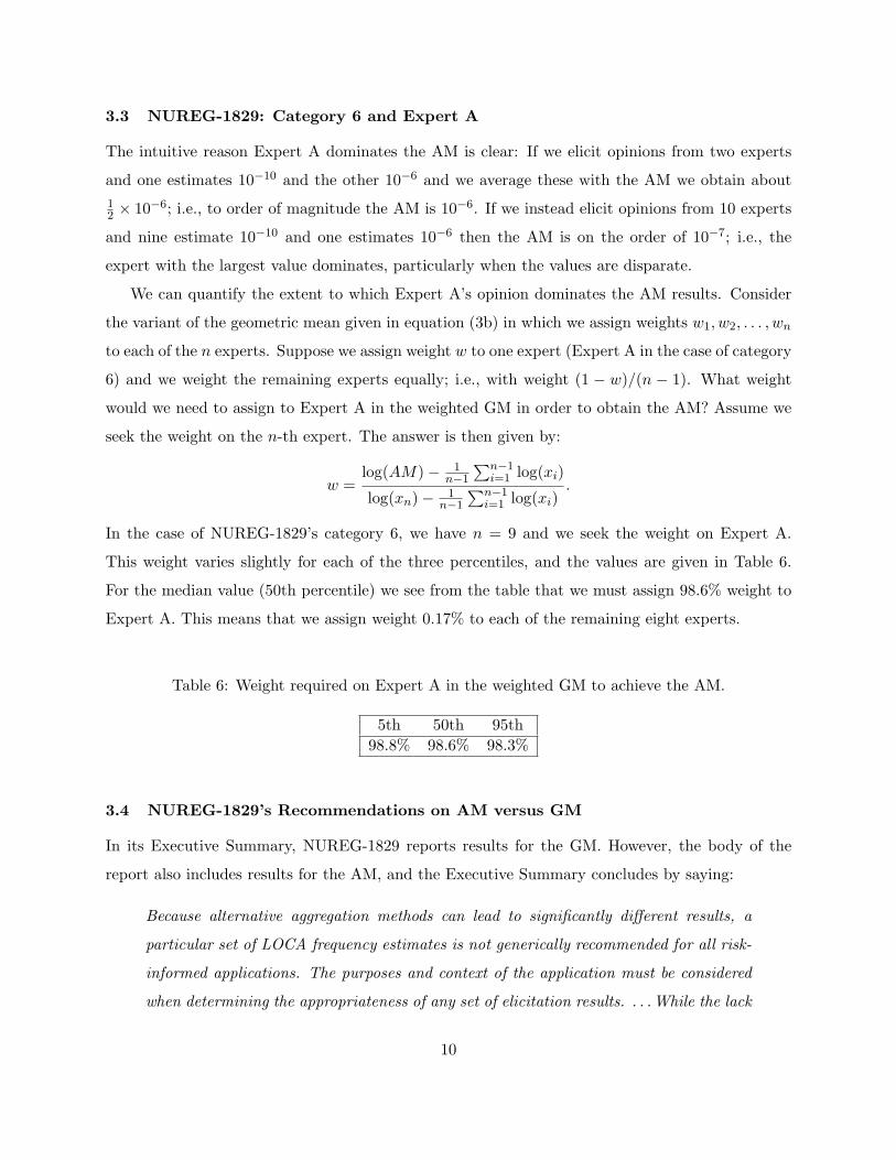
3.3 NUREG-1829: Category 6 and Expert A

The intuitive reason Expert A dominates the AM is clear: If we elicit opinions from two experts

and one estimates 10−10 and the other 10−6 and we average these with the AM we obtain about12 × 10−6; i.e., to order of magnitude the AM is 10−6. If we instead elicit opinions from 10 experts

and nine estimate 10−10 and one estimates 10−6 then the AM is on the order of 10−7; i.e., the

expert with the largest value dominates, particularly when the values are disparate.

We can quantify the extent to which Expert A’s opinion dominates the AM results. Consider

the variant of the geometric mean given in equation (3b) in which we assign weights w1, w2, . . . , wn

to each of the n experts. Suppose we assign weight w to one expert (Expert A in the case of category

6) and we weight the remaining experts equally; i.e., with weight (1 − w)/(n − 1). What weight

would we need to assign to Expert A in the weighted GM in order to obtain the AM? Assume we

seek the weight on the n-th expert. The answer is then given by:

w =log(AM)− 1

n−1

∑n−1i=1 log(xi)

log(xn)− 1n−1

∑n−1i=1 log(xi)

.

In the case of NUREG-1829’s category 6, we have n = 9 and we seek the weight on Expert A.

This weight varies slightly for each of the three percentiles, and the values are given in Table 6.

For the median value (50th percentile) we see from the table that we must assign 98.6% weight to

Expert A. This means that we assign weight 0.17% to each of the remaining eight experts.

Table 6: Weight required on Expert A in the weighted GM to achieve the AM.

5th 50th 95th98.8% 98.6% 98.3%

3.4 NUREG-1829’s Recommendations on AM versus GM

In its Executive Summary, NUREG-1829 reports results for the GM. However, the body of the

report also includes results for the AM, and the Executive Summary concludes by saying:

Because alternative aggregation methods can lead to significantly different results, a

particular set of LOCA frequency estimates is not generically recommended for all risk-

informed applications. The purposes and context of the application must be considered

when determining the appropriateness of any set of elicitation results. . . . While the lack

10

of clear application guidance places an additional burden on the users of the study results,

those users are in the best position to judge which study results are most appropriate to

consider for their particular applications.

We see the above quote as consistent with the notion of a risk-informed, rather than a risk-based,

analysis. Large effective break sizes dominate failure scenarios in STP’s risk-informed approach to

GSI-191. A natural sensitivity analysis that we can perform would answer the question: What

weight must be placed on Expert A, using the ideas in Section 3.3, in order to depart Region III?

Despite the above caveat NUREG-1829 contains in its Executive Summary, the body of NUREG-

1829, along with the literature on combining expert opinion, makes a strong case for using GM

rather than AM at least when: (i) the elicited probabilities concern rare-event probabilities, (ii) the

opinions of the individual experts are disparate, and (iii) we seek a combination rule that represents

a reasonable notion of the center of the group’s opinion. NUREG-1829 recasts (iii) by saying that

validity of the GM aggregation scheme, i.e., the validity of seeking a reasonable notion of the center,

assumes no systematic bias:

A basic premise in using an elicitation process is that the panel responses as a whole

have no significant systematic bias. While individual responses can be highly uncertain

and differ drastically, they do not systematically over- or underestimate the quantities

of interest. Many elements of the elicitation procedure are designed to achieve this goal.

NUREG-1829 goes on to say:

A consequence of the assumption of no systematic bias is that the group estimate should

be somewhere in the middle of the individual estimates, especially if there are wide

differences in the results.

As we have also observed in Section 3, NUREG-1829 notes:

. . . the AM of individual estimates is often not a good measure of the median group

opinion when the individual estimates are widely varying. In this case, the AM is

dominated by the one or two largest results and cannot be fairly described as a group

estimate.

On reasonable notions of the center of the group’s opinions, NUREG-1829 indicates:

There is support for the use of the median or GM in the literature.

11

In previous NRC applications . . . the median was used as a group estimate when the

individual estimates varied by several orders of magnitude.

NUREG-1829 points to Meyer and Booker [6], who say:

To overcome the influence of extreme values when forming an aggregation estimate, use

the median or geometric mean.

NUREG-1829 indicates that in their sensitivity analysis the GM and median produced similar

results. This is consistent with the GM results we summarize in Table 4 of Section 3.

In general, Von Winterfeldt and Edwards [8] prefer AM-style aggregation, but say:

The only context in which we have any reservations about this conclusion is that of

very low probabilities—for such extreme numbers, we would prefer averaging log odds to

averaging probabilities.

As we discuss in Section 2, averaging logarithms (i.e., averaging exponents) is equivalent to the

GM.

We conclude with a summary statement from NUREG-1829, which we see as fully consistent

with our analysis in Section 3:

Taking these considerations into account, and noting that a sensitivity study showed

that there is little difference between using the median or the GM to aggregate the study

results . . . the GM was chosen as the most appropriate group estimate which utilizes all

the individual estimates.

12

References

[1] Arrow, K. J. (1951). Social Choice and Individual Values. Wiley, New York.

[2] Clement, R. T. and R. L. Winkler (1999). Combining probability distributions from experts in

risk analysis. Risk Analysis 19, 187–203.

[3] Cooke, R. M. (1991). Experts in Uncertainty: Opinion and Subjective Probability in Science.

Oxford University Press, New York.

[4] French, S. (1985). Group consensus probability distributions: A critical survey. In Bayesian

Statistics 2, pp. 183–197. North-Holland, Amsterdam.

[5] Genest, C. and J. V. Zidek (1986). Combining probability distributions: A critique and anno-

tated bibliography. Statistical Science 1, 114–148.

[6] Meyer, M. A. and J. M. Booker (1990). Eliciting and Analyzing Expert Judgment: A Practical

Guide, NUREG/CR-5424, U.S. Nuclear Regulatory Commission.

[7] Tregoning, R., L. Abramson, and P. Scott (2008). Estimating Loss-of-Coolant Accident (LOCA)

Frequencies Through the Elicitation Process, NUREG-1829, Volume 1, Nuclear Regulatory Com-

mission, Washington, DC.

[8] Von Winterfeldt, D. and W. Edwards (1986). Decision Analysis and Behavioral Research.

Cambridge University Press, New York, NY.

13