8-1

ME 305 Fluid Mechanics I

Chapter 8

Viscous Flow in Pipes and Ducts

These presentations are prepared by

Dr. Cüneyt Sert

Department of Mechanical Engineering

Middle East Technical University

Ankara, Turkey

csert@metu.edu.tr

You can get the most recent version of this document from Dr. Sert’s web site.

Please ask for permission before using them to teach. You are NOT allowed to modify them.

Flow in Pipes and Ducts

• Flow in closed conduits (circular pipes and non-circular ducts) are very common.

8-2

Flow in Pipes and Ducts (cont’d)

• We assume that pipes/ducts are completely filled with fluid. Other case is known as open channel flow.

• Typical systems involve pipes/ducts of various sizes connected to each other by various fittings, elbows, tees, etc.

• Valves are used to control flow rate.

• Fluid is usually forced to flow by a fan or a pump.

• We need to perform frictional head loss (pressure drop)calculations. They mostly depend on experimental resultsand empirical relations.

• First we need to be able to differentiatebetween laminar and turbulent flows.

8-3

• Laminar flow is characterized by smooth streamlines and highly ordered motion. Fluid flows as if there are immiscible layers of fluid.

• Turbulent flow is highly disordered. Usually there are unsteady, random fluctuations on top of a mean flow.

• Most flows encountered in practice are turbulent.

Laminar vs. Turbulent Flows

𝐷

𝜈

Pipe

𝑄 = 𝑉𝐴

𝑅𝑒𝐷 =𝑉𝐷

𝜈=𝜌𝑉𝐷

𝜇

Laminar

Transitional

Turbulent

Movies

Reynolds Experiment

Laminar vs. Turbulent Velocity Profiles

8-4

• For pipe flow, transition from laminar to turbulent flow occurs at a critical Reynolds number of approximately 2300.

𝑅𝑒𝐷 < 2300 : Laminar

𝑅𝑒𝐷 > 2300 : Turbulent

𝑅𝑒 =Inertia forces

Viscous forces=

𝑉𝐷

𝜈

• At large Reynolds numbers, inertia forces, which are proportional to 𝜌𝑉2𝐷2, are much higher than the viscous forces. Viscous forces can not regularize random fluctuations. Fluctuations grow and the flow becomes turbulent.

• At low Reynolds numbers, viscous forces are high enough to suppress random fluctuations and keep the flow in order, i.e. laminar.

Exercise : Estimate the typical Reynolds number of the flow inside the pipe that supplies water to your shower.

Laminar vs. Turbulent Flows (cont’d)

Characteristic speed(average speed in the pipe)

Characteristic length(pipe diameter)

8-5

• As a fluid flows in a straight, constant diameter pipe its pressure drops due to viscous effects, known as major pressure loss.

• Additional pressure drops occur due to other components such as valves, bends, tees, sudden expansions, sudden contractions, etc. These are known as minor pressure losses.

• In Chapter 6 we studied analytical solution of Hagen-Poiseuille flow, which is the steady, fully-developed, laminar flow in a circular pipe.

• We showed that𝑑𝑝

𝑑𝑥= constant and pressure drop over a pipe section of length 𝐿 is

Δ𝑝 = 𝑓𝐿

𝐷

𝜌𝑉2

2

where 𝑓 = 64/𝑅𝑒𝐷 for laminar flow, with 𝑅𝑒𝐷 =𝑉𝐷

𝜈.

Pressure Loss (Pressure Drop, Head Loss) in Pipe Flow

Darcy friction factor

Dynamic pressure

8-6

Average speed

• Consider the EBE between sections 1 and 2.

𝑝1𝜌𝑔

+𝑉12

2𝑔+ 𝑧1 =

𝑝2𝜌𝑔

+𝑉22

2𝑔+ 𝑧2 + ℎ𝑓

• Friction head is related to the pressure drop as

ℎ𝑓 =Δ𝑝

𝜌𝑔= 𝑓

𝐿

𝐷

𝑉2

2𝑔

• The above important equation is known as the Darcy-Weisbach equation.

Major Pressure Loss in Laminar Pipe Flow

flow 𝐷

1 2𝐿

Δ𝑝 = 𝑓𝐿

𝐷

𝜌𝑉2

2

8-7

• Analytical solution of pipe flow is available only for laminar flows.

• It is not possible to solve Navier-Stokes equations analytically for turbulent flows.

• Instead we need to determine pressure drop values experimentally.

• For a turbulent pipe flow pressure drop depends on

Δ𝑝 = Δ𝑝 𝐿, 𝐷, 𝑉, 𝜇, 𝜌, 𝜀

• A Buckingham-Pi analysis yields the following relation

Δ𝑝

𝜌𝑉2/2= 𝐹

𝐿

𝐷, 𝑅𝑒𝐷,

𝜀

𝐷

which can be expressed in the same way as laminar flow Δ𝑝 = 𝑓 𝑅𝑒𝐷,𝜀

𝐷

𝐿

𝐷

𝜌𝑉2

2

Major Pressure Loss in Turbulent Pipe Flow

New parameter: Surface roughness

8-8

• For a turbulent pipe flow, friction factor is a function of Reynolds number and relative surface roughness.

𝑓 𝑅𝑒𝐷 ,𝜀

𝐷

• In 1933 Nikuradse performed detailed experiments to determine friction factor for turbulent pipe flows.

• Later Colebrook presented this experimental data as the following equation

Colebrook Formula ∶1

𝑓= −2 log

𝜀/𝐷

3.7+

2.51

𝑅𝑒𝐷 𝑓

• An easy to use graphical representation of this equation is known as the Moody diagram, given in the next slide).

• Be careful in reading the logarithmic horizontal and vertical axes of the Moody diagram.

Major Pressure Loss in Turbulent Pipe Flow (cont’d)

Relative surface roughness

8-9

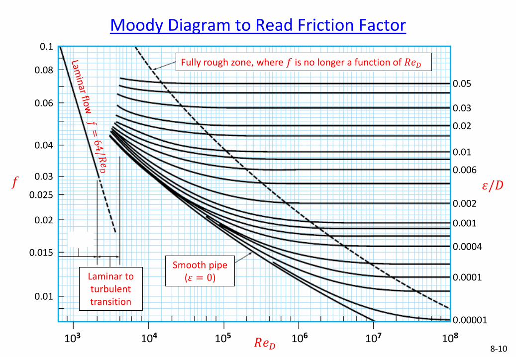
Moody Diagram to Read Friction Factor

0.05

0.03

0.02

0.01

0.006

0.002

0.001

0.0004

0.0001

0.00001

0.1

0.08

0.06

0.04

0.025

0.015

0.01

0.02

0.03

103 104 105 106 107 108

𝑓 𝜀/𝐷

𝑅𝑒𝐷

Fully rough zone, where 𝑓 is no longer a function of 𝑅𝑒𝐷

Laminar to turbulent transition

Smooth pipe (𝜀 = 0)

8-10

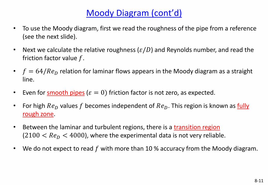
Moody Diagram (cont’d)

• To use the Moody diagram, first we read the roughness of the pipe from a reference(see the next slide).

• Next we calculate the relative roughness (𝜀/𝐷) and Reynolds number, and read the friction factor value 𝑓.

• 𝑓 = 64/𝑅𝑒𝐷 relation for laminar flows appears in the Moody diagram as a straight line.

• Even for smooth pipes (𝜀 = 0) friction factor is not zero, as expected.

• For high 𝑅𝑒𝐷 values 𝑓 becomes independent of 𝑅𝑒𝐷. This region is known as fullyrough zone.

• Between the laminar and turbulent regions, there is a transition region(2100 < 𝑅𝑒𝐷 < 4000), where the experimental data is not very reliable.

• We do not expect to read 𝑓 with more than 10 % accuracy from the Moody diagram.

8-11

Moody Diagram (cont’d)

8-12

For pipes which are in servicefor a long time, roughnessvalues given in tables for newpipes should be used withcaution.

• As an alternative to the Moody diagram, Haaland’s equation (explicit and easy to use)can be used to calculate 𝑓.

1

𝑓= −1.8 log

𝜀/𝐷

3.7

1.11

+6.9

𝑅𝑒𝐷

Major Head Loss Exercise

Exercise : Crude oil flows through a level section of a pipeline at a rate of 2.944 m3/s. The pipe inside diameter is 1.22 m, its roughness is equivalent to galvanized iron. The maximum allowable pressure is 8.27 MPa. The minimum pressure required to keep dissolved gases in solution in the crude oil is 344.5 kPa. The crude oil has a specific gravity of 0.93. Viscosity at the pumping temperature of 60 ℃ is𝜇 = 0.0168 Pa s. a) Determine the maximum allowable spacing between the pumping stations. b) If the pump efficiency is 85%, determine the power that must be supplied at each pumping station. (Reference: Fox’s book)

8-13

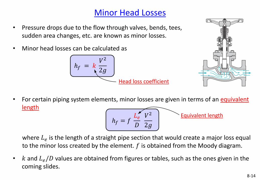
Minor Head Losses

• Pressure drops due to the flow through valves, bends, tees,sudden area changes, etc. are known as minor losses.

• Minor head losses can be calculated as

ℎ𝑓 = 𝑘𝑉2

2𝑔

• For certain piping system elements, minor losses are given in terms of an equivalent length

ℎ𝑓 = 𝑓𝐿𝑒𝐷

𝑉2

2𝑔

where 𝐿𝑒 is the length of a straight pipe section that would create a major loss equal to the minor loss created by the element. 𝑓 is obtained from the Moody diagram.

• 𝑘 and 𝐿𝑒/𝐷 values are obtained from figures or tables, such as the ones given in the coming slides.

Head loss coefficient

8-14

Equivalent length

8-15

Minor Head Losses (cont’d)

Fox’s book

ℎ𝑓 = 𝑘ത𝑉2

2𝑔, where ത𝑉 is the average veocity in the pipe

8-16

Minor Head Losses (cont’d)

Fox’s book

ℎ𝑓 = 𝑘𝑐ത𝑉22

2𝑔ℎ𝑓 = 𝑘𝑒

ത𝑉12

2𝑔

8-17

Minor Head Losses (cont’d)

Fox’s book

ℎ𝑓 = 𝑘ത𝑉22

2𝑔

8-18

Minor Head Losses (cont’d)

Fox’s book

ℎ𝑓 = 𝑓𝐿𝑒𝐷

𝑉2

2𝑔

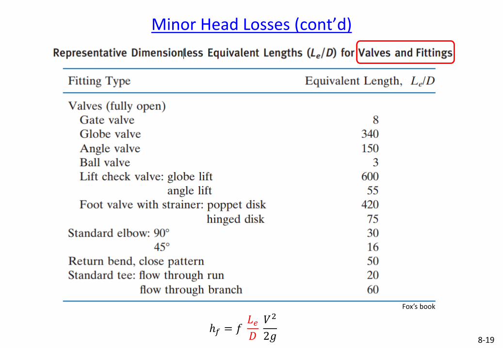
8-19

Minor Head Losses (cont’d)

Fox’s book

ℎ𝑓 = 𝑓𝐿𝑒𝐷

𝑉2

2𝑔

Examples (cont’d)

Exercise : Sketch of the warm water heating system of a studio apartment is shown in the figure. Volumetric flow rate of water through the piping system with a diameter of 1.25 cm is 0.2 L/s. Friction factor is 0.02. Head loss coefficients for the elbow, heater valve, radiator, gate valve and boiler are 2.0, 5.0, 3.0, 1.0 and 3.0, respectively. Determine the power required to drive the circulation pump, which has an efficiency of 75%.

Radiator

Heater valve

Gate valves

Pump

Elbow Elbow

ElbowBoiler

10 m

1 m

8 m

8-20

Examples (cont’d)

• Some problems require an iterative solution because 𝑅𝑒𝐷 and 𝑓 cannot be computed directly. Solution starts with an initial guess for 𝑓 and/or 𝐷. Usually couple of iterations are enough to get the final answer.

• Typical problems of this sort are

• 𝐿 and 𝐷 of the pipe are known. Find 𝑄 for a specified ∆𝑝.

If 𝑄 is not known, 𝑅𝑒𝐷, 𝑓 and ℎ𝑓 cannot be calculated directly.

• 𝐿 of the pipe is known. Find 𝐷 for a specified 𝑄 and ∆𝑝.

If 𝐷 is not known, 𝑅𝑒𝐷, 𝑓 and ℎ𝑓 cannot be calculated directly.

• Problems with multiple branches.

If 𝑄 passing from each branch is not known, 𝑅𝑒𝐷, 𝑓 and ℎ𝑓 cannot be

calculated directly.

Exercise : Air at 1 atm and 35 ℃ is to be transported in a 150 m long plastic pipe at a rate of 0.35 m3/s. If the head loss in the pipe is not to exceed 20 m, determine the minimum diameter of the duct.

8-21

Exercise : Consider the previous exercise again. Now the duct length is doubled while its diameter is kept constant. If the total head loss is to remain constant, determine the new flow rate through the duct.

Exercise : A swimming pool has a partial-flow filtration system. Water at 24 ℃ is pumped from the pool through the system shown. The pump delivers 1.9 L/s. The pipes are made of PVC with internal diameters of 21 mm). The pressure loss through the filter is given as Δ𝑝 = 1039 𝑄2, where Δ𝑝 is in kPa and 𝑄 is in L/s. Determine the pump pressure and the flow rate through each branch of the system(Reference: Fox’s book).

8-22

Examples (cont’d)

Non-Circular Geometries – Hydraulic Diameter

• Correlations derived for circular pipes can be used for non-circular (rectangle, triangle, trapezoid, etc.) ducts, provided that the cross sections do not have very high ascpect ratios.

• Ducts with square or rectangular cross sections can be treated if their height to width ratio is less than about 3 or 4.

• To do this we use the hydraulic diameter concept

𝐷ℎ =4𝐴

𝑃

8-23

Cross sectional area of the duct

Perimeter of the duct

𝑎

𝑏 𝐷ℎ =4(𝑎𝑏)

2(𝑎 + 𝑏)is equivalent to

𝐷ℎ