MCMC Chapter

8/3/2019 MCMC Chapter

http://slidepdf.com/reader/full/mcmc-chapter 1/39

Machine Learning, 50, 5–43, 2003

c 2003 Kluwer Academic Publishers. Manufactured in The Netherlands.

An Introduction to MCMC for Machine Learning

CHRISTOPHE ANDRIEU [email protected]

Department of Mathematics, Statistics Group, University of Bristol, University Walk, Bristol BS8 1TW, UK

NANDO DE FREITAS [email protected]

Department of Computer Science, University of British Columbia, 2366 Main Mall, Vancouver,

BC V6T 1Z4, Canada

ARNAUD DOUCET [email protected] Department of Electrical and Electronic Engineering,Universityof Melbourne, Parkville, Victoria 3052, Australia

MICHAEL I. JORDAN [email protected]

Departments of Computer Science and Statistics, University of California at Berkeley, 387 Soda Hall, Berkeley,

CA 94720-1776, USA

Abstract. This purpose of this introductory paper is threefold. First, it introduces the Monte Carlo method with

emphasis on probabilistic machine learning. Second, it reviews the main building blocks of modern Markov chain

Monte Carlo simulation, thereby providing and introduction to the remaining papers of this special issue. Lastly,

it discusses new interesting research horizons.

Keywords: Markov chain Monte Carlo, MCMC, sampling, stochastic algorithms

1. Introduction

A recent survey places the Metropolis algorithm among the ten algorithms that have had the

greatest influence on the development and practice of science and engineering in the 20th

century (Beichl & Sullivan, 2000). This algorithm is an instance of a large class of sampling

algorithms, known as Markov chain Monte Carlo (MCMC). These algorithms have played

a significant role in statistics, econometrics, physics and computing science over the last

two decades. There are several high-dimensional problems, such as computing the volume

of a convex body in d dimensions, for which MCMC simulation is the only known general

approach for providing a solution within a reasonable time (polynomial in d ) (Dyer, Frieze,

& Kannan, 1991; Jerrum & Sinclair, 1996).While convalescing from an illness in 1946, Stan Ulam was playing solitaire. It, then,

occurred to him to try to compute the chances that a particular solitaire laid out with 52 cards

would come out successfully (Eckhard, 1987). After attempting exhaustive combinatorial

calculations, he decided to go for the more practical approach of laying out several solitaires

at random and then observing and counting the number of successful plays. This idea of

selecting a statistical sample to approximate a hard combinatorial problem by a much

simpler problem is at the heart of modern Monte Carlo simulation.



6 C. ANDRIEU ET AL.

Stan Ulam soon realised that computers could be used in this fashion to answer ques-

tions of neutron diffusion and mathematical physics. He contacted John Von Neumann,

who understood the great potential of this idea. Over the next few years, Ulam and Von

Neumann developed many Monte Carlo algorithms, including importance sampling and

rejection sampling. Enrico Fermi in the 1930’s also used Monte Carlo in the calculation of

neutron diffusion, and later designed the FERMIAC, a Monte Carlo mechanical device that

performed calculations (Anderson, 1986). In the 1940’s Nick Metropolis, a young physicist,

designed new controls for the state-of-the-art computer (ENIAC) with Klari Von Neumann,

John’s wife. He was fascinated with Monte Carlo methods and this new computing device.

Soon he designed an improved computer, which he named the MANIAC in the hope that

computer scientists would stop using acronyms. During the time he spent working on the

computing machines, many mathematicians and physicists (Fermi, Von Neumann, Ulam,

Teller, Richtmyer, Bethe, Feynman, & Gamow) would go to him with their work problems.Eventually in 1949, he published the first public document on Monte Carlo simulation with

Stan Ulam (Metropolis & Ulam, 1949). This paper introduces, among other ideas, Monte

Carlo particle methods, which form the basis of modern sequential Monte Carlo methods

such as bootstrap filters, condensation, and survival of the fittest algorithms (Doucet, de

Freitas, & Gordon, 2001). Soon after, he proposed the Metropolis algorithm with the Tellers

and the Rosenbluths (Metropolis et al., 1953).

Many papers on Monte Carlo simulation appeared in the physics literature after 1953.

From an inference perspective, the most significant contribution was the generalisation of

the Metropolis algorithm by Hastings in 1970. Hastings and his student Peskun showed that

Metropolis and the more general Metropolis-Hastings algorithms are particular instances

of a large family of algorithms, which also includes the Boltzmann algorithm (Hastings,

1970; Peskun, 1973). They studied the optimality of these algorithms and introduced the

formulation of the Metropolis-Hastings algorithm that we adopt in this paper. In the 1980’s,

two important MCMC papers appeared in the fields of computer vision and artificial in-

telligence (Geman & Geman, 1984; Pearl, 1987). Despite the existence of a few MCMC

publications in the statistics literature at this time, it is generally accepted that it was only in

1990 that MCMC made the first significant impact in statistics (Gelfand & Smith, 1990). In

the neural networks literature, the publication of Neal (1996) was particularly influential.

In the introduction to this special issue, we focus on describing algorithms that we feel

are the main building blocks in modern MCMC programs. We should emphasize that in

order to obtain the best results out of this class of algorithms, it is important that we do not

treat them as black boxes, but instead try to incorporate as much domain specific knowledge

as possible into their design. MCMC algorithms typically require the design of proposal

mechanisms to generate candidate hypotheses. Many existing machine learning algorithms

can be adapted to become proposal mechanisms (de Freitas et al., 2001). This is oftenessential to obtain MCMC algorithms that converge quickly. In addition to this, we believe

that the machine learning community can contribute significantly to the solution of many

open problems in the MCMC field. For this purpose, we have outlined several “hot” research

directions at the end of this paper. Finally, readers are encouraged to consult the excellent

texts of Chen, Shao, and Ibrahim (2001), Gilks, Richardson, and Spiegelhalter (1996), Liu

(2001), Meyn and Tweedie (1993), Robert and Casella (1999) and review papers by Besag



INTRODUCTION 7

et al. (1995), Brooks (1998), Diaconis and Saloff-Coste (1998), Jerrum and Sinclair (1996),

Neal (1993), and Tierney (1994) for more information on MCMC.

The remainder of this paper is organised as follows. In Part 2, we outline the general

problems and introduce simple Monte Carlo simulation, rejection sampling and importance

sampling. Part 3 deals with the introduction of MCMC and the presentation of the most

popular MCMC algorithms. In Part 4, we describe some important research frontiers. To

make the paper more accessible, we make no notational distinction between distributions

and densities until the section on reversible jump MCMC.

2. MCMC motivation

MCMC techniques are often applied to solve integration and optimisation problems in

large dimensional spaces. These two types of problem play a fundamental role in machinelearning, physics, statistics, econometrics and decision analysis. The following are just some

examples.

1. Bayesian inference and learning. Given some unknown variables x ∈ X and data y ∈ Y ,the following typically intractable integration problems are central to Bayesian statistics

(a) Normalisation. To obtain the posterior p( x | y) given the prior p( x) and likelihood

p( y | x), the normalising factor in Bayes’ theorem needs to be computed

p( x | y) = p( y | x ) p( x) X p( y | x ) p( x ) d x .

(b) Marginalisation. Given the joint posterior of ( x, z) ∈ X × Z , we may often be

interested in the marginal posterior

p( x | y) = Z

p( x, z | y) dz.

(c) Expectation. The objective of the analysis is often to obtain summary statistics of

the form

E p( x| y)( f ( x)) = X

f ( x) p( x | y) d x

for some function of interest f : X → Rn f integrable with respect to p( x | y).

Examples of appropriate functions include the conditional mean, in which case

f ( x) = x , or theconditionalcovarianceof x where f ( x) = xx−E p( x| y)( x)E p( x| y)( x).

2. Statistical mechanics. Here, one needs to compute the partition function Z of a system

with states s and Hamiltonian E (s)

Z =

s

exp

− E (s)

kT

,

where k is the Boltzmann’s constant and T denotes the temperature of the system.

Summing over the large number of possible configurations is prohibitively expensive

(Baxter, 1982). Note that the problems of computing the partition function and the

normalising constant in statistical inference are analogous.



8 C. ANDRIEU ET AL.

3. Optimisation. The goal of optimisation is to extract the solution that minimises some

objective function from a large set of feasible solutions. In fact, this set can be contin-

uous and unbounded. In general, it is too computationally expensive to compare all the

solutions to find out which one is optimal.

4. Penalised likelihood model selection. This task typically involves two steps. First, one

finds the maximum likelihood (ML) estimates for each model separately. Then one uses

a penalisation term (for example MDL, BIC or AIC) to select one of the models. The

problem with this approach is that the initial set of models can be very large. Moreover,

many of those models are of not interest and, therefore, computing resources are wasted.

Although we have emphasized integration and optimisation, MCMC also plays a funda-

mental role in the simulation of physical systems. This is of great relevance in nuclear

physics and computer graphics (Chenney & Forsyth, 2000; Kalos & Whitlock, 1986; Veach& Guibas, 1997).

2.1. The Monte Carlo principle

The idea of Monte Carlo simulation is to draw an i.i.d. set of samples { x (i )} N i=1 from a target

density p( x) defined on a high-dimensional space X (e.g. the set of possible configurations

of a system, the space on which the posterior is defined, or the combinatorial set of feasible

solutions). These N samples canbe used to approximate thetarget density with thefollowing

empirical point-mass function

p N ( x)

=

1

N

N

i=1

δ x (i ) ( x),

where δ x (i ) ( x ) denotes the delta-Dirac mass located at x (i ). Consequently, one can approx-

imate the integrals (or very large sums) I ( f ) with tractable sums I N ( f ) that converge as

follows

I N ( f ) = 1

N

N i=1

f x (i )

a.s.−−−→ N →∞

I ( f ) = X

f ( x) p( x) d x .

That is, the estimate I N ( f ) is unbiased and by the strong law of large numbers, it will

almost surely (a.s.) converge to I ( f ). If the variance (in the univariate case for simplicity)

of f ( x) satisfies σ 2 f E p( x )( f 2( x)) − I 2( f ) < ∞, then the variance of the estimator

I N ( f ) is equal to var( I N ( f )) =σ 2 f

N and a central limit theorem yields convergence indistribution of the error

√ N ( I N ( f ) − I ( f )) =⇒

N →∞ N

0, σ 2 f

,

where =⇒ denotes convergence in distribution (Robert & Casella, 1999; Section 3.2).

The advantage of Monte Carlo integration over deterministic integration arises from the

fact that the former positions the integration grid (samples) in regions of high probability.



INTRODUCTION 9

The N samples can also be used to obtain a maximum of the objective function p( x) as

follows

ˆ x = arg max x (i );i=1,..., N

p x (i )

However, we will show later that it is possible to construct simulated annealing algorithms

that allow us to sample approximately from a distribution whose support is the set of global

maxima.

When p( x ) has standard form, e.g. Gaussian, it is straightforward to sample from it using

easily available routines. However, when this is not the case, we need to introduce more

sophisticated techniques based on rejection sampling, importance sampling and MCMC.

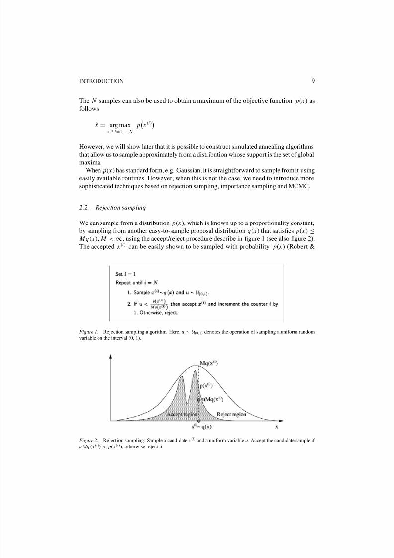
2.2. Rejection sampling

We can sample from a distribution p( x ), which is known up to a proportionality constant,

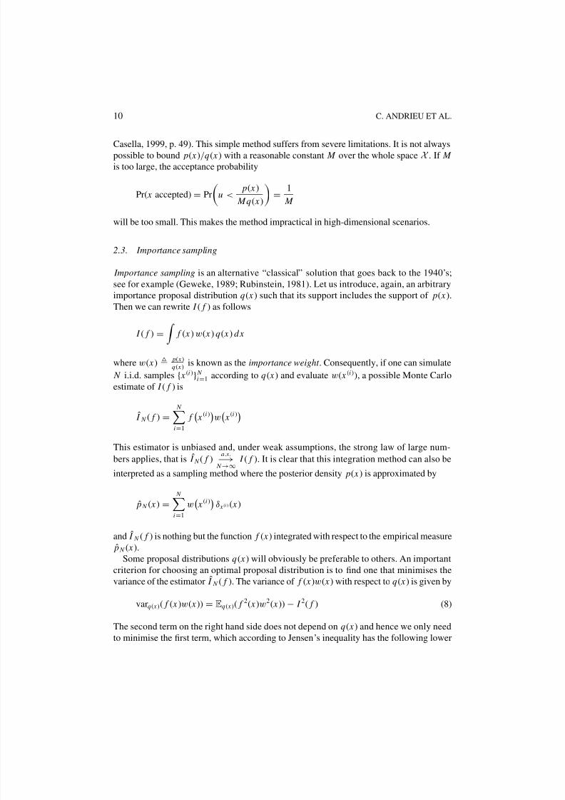
by sampling from another easy-to-sample proposal distribution q( x) that satisfies p( x) ≤ Mq( x), M < ∞, using the accept/reject procedure describe in figure 1 (see also figure 2).

The accepted x (i ) can be easily shown to be sampled with probability p( x ) (Robert &

Figure 1. Rejection sampling algorithm. Here, u ∼ U (0,1) denotes the operation of sampling a uniform random

variable on the interval (0, 1).

Figure 2. Rejection sampling: Sample a candidate x (i ) and a uniform variable u. Accept the candidate sample if

u Mq ( x (i )) < p( x (i )), otherwise reject it.



10 C. ANDRIEU ET AL.

Casella, 1999, p. 49). This simple method suffers from severe limitations. It is not always

possible to bound p( x)/q( x ) with a reasonable constant M over the whole space X . If M

is too large, the acceptance probability

Pr( x accepted) = Pr

u <

p( x )

Mq( x)

= 1

M

will be too small. This makes the method impractical in high-dimensional scenarios.

2.3. Importance sampling

Importance sampling is an alternative “classical” solution that goes back to the 1940’s;

see for example (Geweke, 1989; Rubinstein, 1981). Let us introduce, again, an arbitrary

importance proposal distribution q( x ) such that its support includes the support of p( x).

Then we can rewrite I ( f ) as follows

I ( f ) =

f ( x ) w( x ) q( x) d x

where w( x) p( x)

q( x)is known as the importance weight . Consequently, if one can simulate

N i.i.d. samples { x (i )} N i=1 according to q( x) and evaluate w( x (i )), a possible Monte Carlo

estimate of I ( f ) is

ˆ I N ( f ) =

N i=1

f x

(i )w x

(i )This estimator is unbiased and, under weak assumptions, the strong law of large num-

bers applies, that is ˆ I N ( f )a.s.−→

N →∞ I ( f ). It is clear that this integration method can also be

interpreted as a sampling method where the posterior density p( x) is approximated by

ˆ p N ( x ) = N

i=1

w x (i )

δ x (i ) ( x)

and ˆ I N ( f ) is nothing but the function f ( x) integrated with respect to the empirical measure

ˆ p N ( x).

Some proposal distributions q( x) will obviously be preferable to others. An importantcriterion for choosing an optimal proposal distribution is to find one that minimises the

variance of the estimator ˆ I N ( f ). The variance of f ( x)w( x) with respect to q( x) is given by

varq( x)( f ( x )w( x)) = Eq( x)( f 2( x)w2( x)) − I 2( f ) (8)

The second term on the right hand side does not depend on q( x) and hence we only need

to minimise the first term, which according to Jensen’s inequality has the following lower



INTRODUCTION 11

bound

Eq( x)( f 2( x )w2( x)) ≥Eq( x )(| f ( x)|w( x))

2 =

| f ( x)| p( x) d x

2

This lower bound is attained when we adopt the following optimal importance distribution

q ( x) = | f ( x)| p( x) | f ( x)| p( x) d x

The optimal proposal is not very useful in the sense that it is not easy to sample from

| f ( x )| p( x ). However, it tells us that high sampling ef ficiency is achieved when we focus

on sampling from p( x) in the important regions where | f ( x)| p( x) is relatively large; hencethe name importance sampling.

This result implies that importance sampling estimates can be super-ef ficient. That is,

for a a given function f ( x), it is possible to find a distribution q( x ) that yields an estimate

with a lower variance than when using a perfect Monte Carlo method, i.e. with q( x) = p( x).

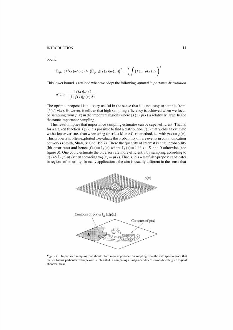
This property is often exploited to evaluate the probability of rare events in communication

networks (Smith, Shafi, & Gao, 1997). There the quantity of interest is a tail probability

(bit error rate) and hence f ( x) = I E ( x) where I E ( x) = 1 if x ∈ E and 0 otherwise (see

figure 3). One could estimate the bit error rate more ef ficiently by sampling according to

q( x) ∝ I E ( x) p( x) than according to q( x) = p( x). That is, it is wasteful to propose candidates

in regions of no utility. In many applications, the aim is usually different in the sense that

Figure 3. Importance sampling: one should place more importance on sampling from the state space regions that

matter. In this particular example one is interested in computing a tail probability of error (detecting infrequent

abnormalities).




one wants to have a good approximation of p( x) and not of a particular integral with respect

to p( x), so we often seek to have q( x) p( x).

As the dimension of the x increases, it becomes harder to obtain a suitable q( x) from

which to draw samples. A sensible strategy is to adopt a parameterised q( x, θ ) and to

adapt θ during the simulation. Adaptive importance sampling appears to have originated

in the structural safety literature (Bucher, 1988), and has been extensively applied in the

communications literature (Al-Qaq, Devetsikiotis, & Townsend, 1995; Remondo et al.,

2000). This technique has also been exploited recently in the machine learning community

(de Freitas et al., 2000; Cheng & Druzdzel, 2000; Ortiz & Kaelbling, 2000; Schuurmans &

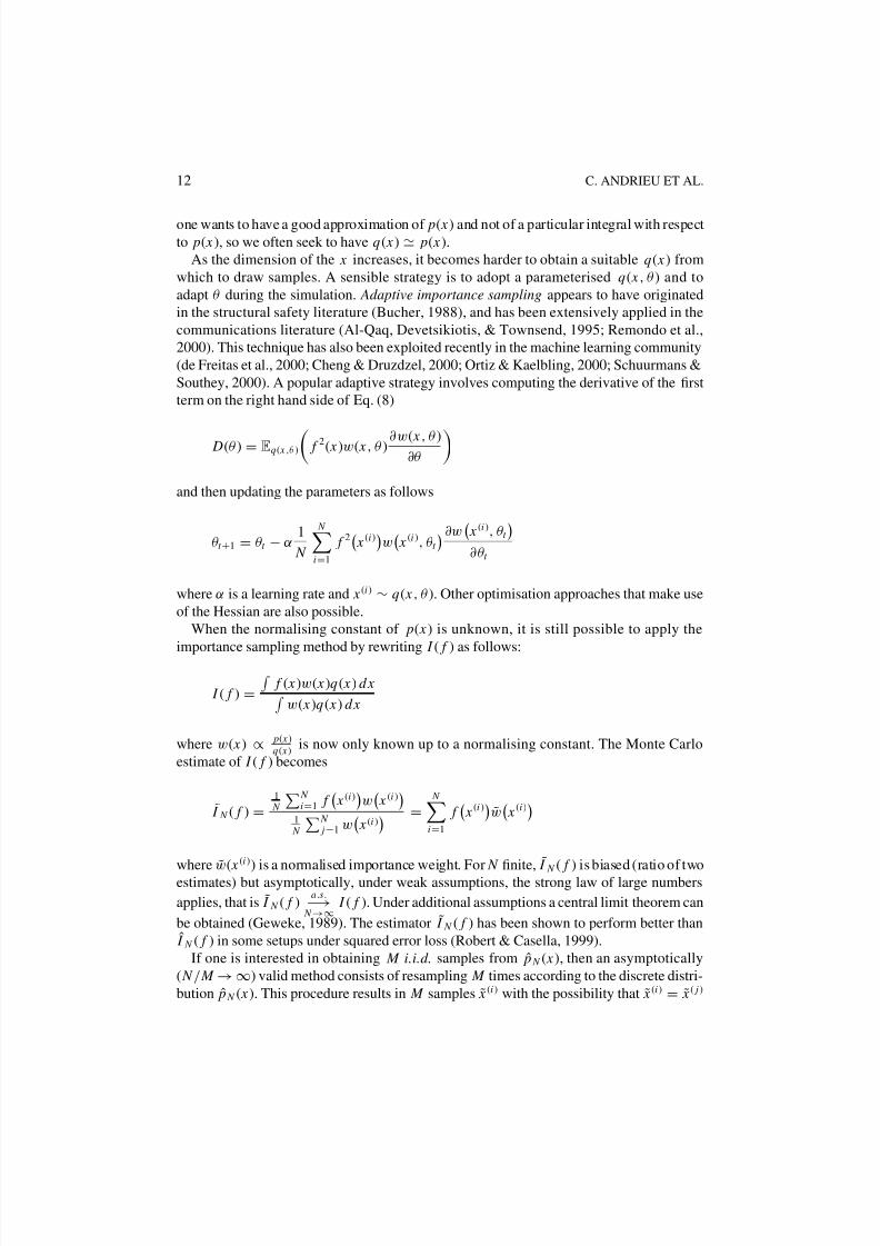
Southey, 2000). A popular adaptive strategy involves computing the derivative of the first

term on the right hand side of Eq. (8)

D(θ ) = Eq( x ,θ)

f 2( x)w( x, θ ) ∂w( x , θ )

∂θ

and then updating the parameters as follows

θt +1 = θt − α1

N

N i=1

f 2 x (i)

w x (i ), θt

∂w x (i ), θt

∂θt

where α is a learning rate and x (i ) ∼ q( x , θ ). Other optimisation approaches that make use

of the Hessian are also possible.

When the normalising constant of p( x) is unknown, it is still possible to apply the

importance sampling method by rewriting I ( f ) as follows:

I ( f ) =

f ( x)w( x)q( x) d x w( x)q( x) d x

where w( x) ∝ p( x)

q( x)is now only known up to a normalising constant. The Monte Carlo

estimate of I ( f ) becomes

˜ I N ( f ) =1

N

N i=1 f

x (i)

w x (i )

1

N

N j=1 w

x (i )

= N

i=1

f x (i )

w x (i)

where w( x (i )) is a normalised importance weight. For N finite, ˜ I N

( f ) is biased (ratio of two

estimates) but asymptotically, under weak assumptions, the strong law of large numbers

applies, that is ˜ I N ( f )a.s.−→

N →∞ I ( f ). Under additional assumptions a central limit theorem can

be obtained (Geweke, 1989). The estimator ˜ I N ( f ) has been shown to perform better thanˆ I N ( f ) in some setups under squared error loss (Robert & Casella, 1999).

If one is interested in obtaining M i.i.d. samples from ˆ p N ( x), then an asymptotically

( N / M → ∞) valid method consists of resampling M times according to the discrete distri-

bution ˆ p N ( x). This procedure results in M samples ˜ x (i ) with the possibility that ˜ x (i ) = ˜ x ( j )



INTRODUCTION 13

for i = j . This method is known as sampling importance resampling (SIR) (Rubin, 1988).

After resampling, the approximation of the target density is

˜ p M ( x ) = 1

M

M i=1

δ ˜ x (i ) ( x) (13)

The resampling scheme introduces some additional Monte Carlo variation. It is, therefore,

not clear whether the SIR procedure can lead to practical gains in general. However, in

the sequential Monte Carlo setting described in Section 4.3, it is essential to carry out this

resampling step.

We conclude this section by stating that even with adaptation, it is often impossible to

obtain proposal distributions that are easy to sample from and good approximations at the

same time. For this reason, we need to introduce more sophisticated sampling algorithmsbased on Markov chains.

3. MCMC algorithms

MCMC is a strategy for generating samples x (i ) while exploring the state space X using a

Markov chain mechanism. This mechanism is constructed so that the chain spends more

time in the most important regions. In particular, it is constructed so that the samples x (i )

mimic samples drawn from the target distribution p( x). (We reiterate that we use MCMC

when we cannot draw samples from p( x) directly, but can evaluate p( x) up to a normalising

constant.)

It is intuitive to introduce Markov chains on finite state spaces, where x (i ) can only take

s discrete values x

(i)

∈X = { x1, x2, . . . , xs}. The stochastic process x

(i )

is called a Markovchain if

p x (i )

x (i−1), . . . , x (1)

= T x (i )

x (i−1)

,

Thechainis homogeneousif T T ( x (i ) | x (i−1)) remains invariant forall i ,with

x (i ) T ( x (i ) | x (i−1)) = 1 for any i . That is, the evolution of the chain in a space X depends solely on the

current state of the chain and a fixed transition matrix.

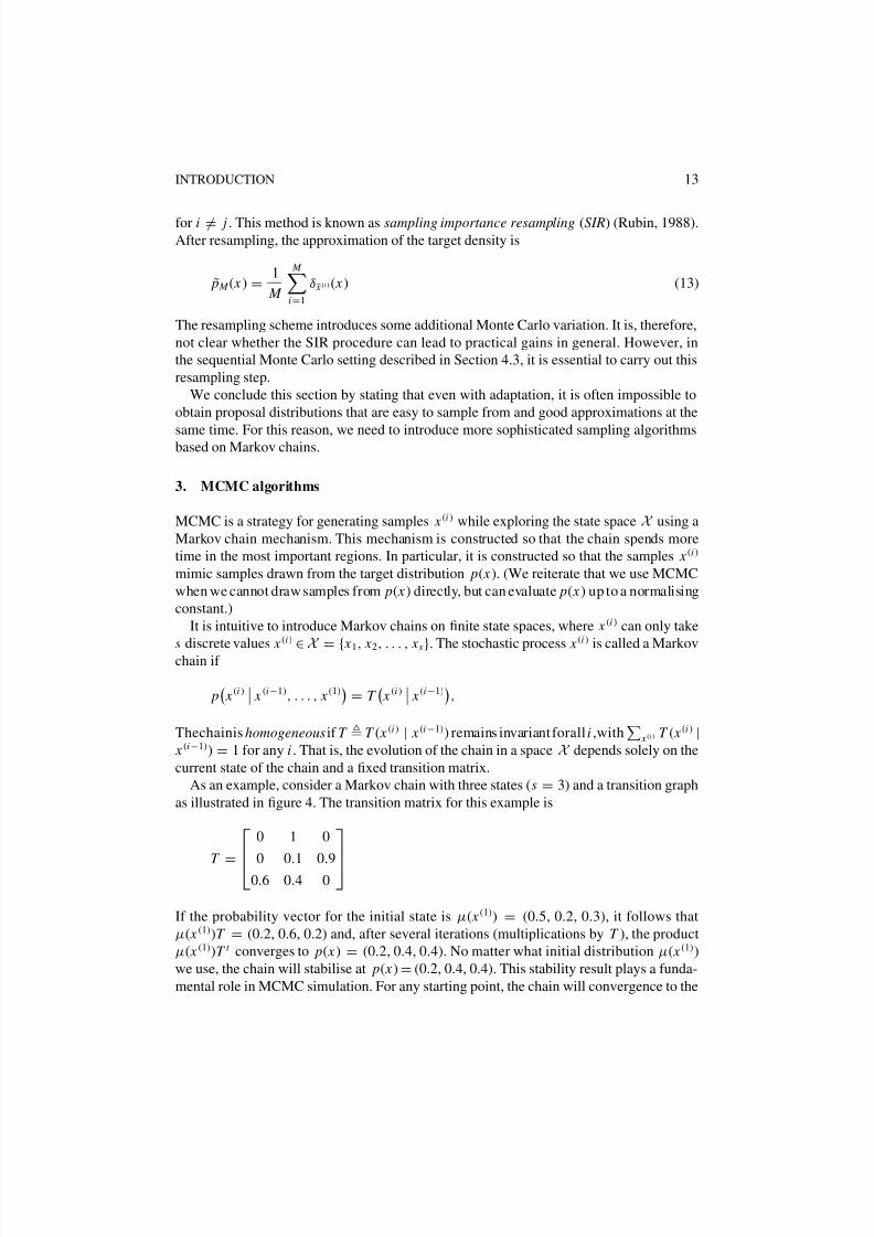
As an example, consider a Markov chain with three states (s = 3) and a transition graph

as illustrated in figure 4. The transition matrix for this example is

T =

0 1 0

0 0.1 0.9

0.6 0.4 0

If the probability vector for the initial state is µ( x (1)) = (0.5, 0.2, 0.3), it follows that

µ( x (1))T = (0.2, 0.6, 0.2) and, after several iterations (multiplications by T ), the product

µ( x (1))T t converges to p( x) = (0.2, 0.4, 0.4). No matter what initial distribution µ( x (1))

we use, the chain will stabilise at p( x) = (0.2, 0.4, 0.4). This stability result plays a funda-

mental role in MCMC simulation. For any starting point, the chain will convergence to the




1

0.6

0.4

0.9

1

2

3x

x

0.1

x

Figure 4. Transition graph for the Markov chain example withX = { x1, x2, x3}.

invariant distribution p( x), as long as T is a stochastic transition matrix that obeys the

following properties:

1. Irreducibility. For any state of the Markov chain, there is a positive probability of visiting

all other states. That is, the matrix T cannot be reduced to separate smaller matrices,

which is also the same as stating that the transition graph is connected.

2. Aperiodicity. The chain should not get trapped in cycles.

A suf ficient, but not necessary, condition to ensure that a particular p( x) is the desiredinvariant distribution is the following reversibility (detailed balance) condition

p x (i )

T x (i−1)

x (i )

= p x (i−1)

T x (i )

x (i−1)

.

Summing both sides over x (i−1), gives us

p x (i )

=

x (i−1)

p x (i−1)

T x (i ) | x (i−1)

.

MCMC samplers are irreducible and aperiodic Markov chains that have the target distribu-

tion as the invariant distribution. One way to design these samplers is to ensure that detailed

balance is satisfied. However, it is also important to design samplers that converge quickly.

Indeed, most of our efforts will be devoted to increasing the convergence speed.Spectral theory gives us useful insights into the problem. Notice that p( x) is the left

eigenvector of the matrix T with corresponding eigenvalue 1. In fact, the Perron-Frobenius

theorem from linear algebra tells us that the remaining eigenvalues have absolute value less

than 1. The second largest eigenvalue, therefore, determines the rate of convergence of the

chain, and should be as small as possible.

The concepts of irreducibility, aperiodicity and invariance can be better appreciated once

we realise the important role that they play in our lives. When we search for information on



INTRODUCTION 15

the World-Wide Web, we typically follow a set of links (Berners-Lee et al., 1994). We can

interpret the webpages and links, respectively, as the nodes and directed connections in a

Markov chain transition graph. Clearly, we (say, the random walkers on the Web) want to

avoid getting trapped in cycles (aperiodicity) and want to be able to access all the existing

webpages (irreducibility). Let us consider, now, the popular information retrieval algorithm

used by the search engine Google, namely PageRank (Page et al., 1998). PageRank requires

the definition of a transition matrix with twocomponents T = L + E . L is a large link matrix

with rows and columns corresponding to web pages, such that the entry L i, j represents the

normalised number of links from web page i to web page j . E is a uniform random matrix

of small magnitude that is added to L to ensure irreducibility and aperiodicity. That is, the

addition of noise prevents us from getting trapped in loops, as it ensures that there is always

some probability of jumping to anywhere on the Web. From our previous discussion, we

have

p x (i+1)

[ L + E ] = p( x i )

where, in this case, the invariant distribution (eigenvector) p( x) represents the rank of a

webpage x . Note that it is possible to design more interesting transition matrices in this

setting. As long as one satisfies irreducibility and aperiodicity, one can incorporate terms

into the transition matrix that favour particular webpages or that bias the search in useful

ways.

In continuous state spaces, the transition matrix T becomes an integral kernel K and

p( x ) becomes the corresponding eigenfunction

p x (i )

K x (i+1)

x (i )

d x (i) = p

x (i+1)

.

The kernel K is the conditional density of x (i+1) given the value x (i ). It is a mathematical

representation of a Markov chain algorithm. In the following subsections we describe

various of these algorithms.

3.1. The Metropolis-Hastings algorithm

The Metropolis-Hastings (MH) algorithm is the most popular MCMC method (Hastings,

1970; Metropolis et al., 1953). In later sections, we will see that most practical MCMC

algorithms can be interpreted as special cases or extensions of this algorithm.

An MH step of invariant distribution p( x ) and proposal distribution q( x

| x) involvessampling a candidate value x given the current value x according to q( x | x). The Markov

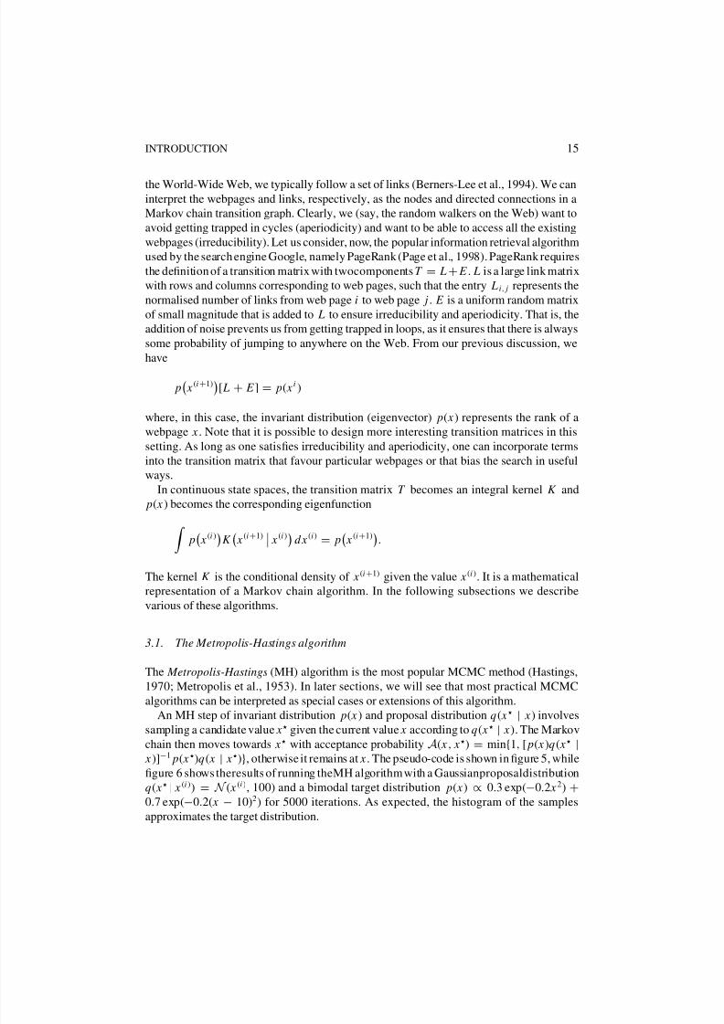
chain then moves towards x with acceptance probability A( x , x ) = min{1, [ p( x)q( x | x )]−1 p( x )q( x | x )}, otherwise it remains at x . The pseudo-code is shown in figure 5, while

figure 6 shows theresults of running theMH algorithm with a Gaussianproposaldistribution

q( x | x (i )) = N ( x (i ), 100) and a bimodal target distribution p( x) ∝ 0.3 exp(−0.2 x 2) +0.7 exp(−0.2( x − 10)2) for 5000 iterations. As expected, the histogram of the samples

approximates the target distribution.




Figure 5. Metropolis-Hastings algorithm.

−10 0 10 200

0.05

0.1

0.15

i=100

−10 0 10 200

0.05

0.1

0.15

i=500

−10 0 10 200

0.05

0.1

0.15

i=1000

−10 0 10 200

0.05

0.1

0.15

i=5000

Figure 6 . Target distribution and histogram of the MCMC samples at different iteration points.

The MH algorithm is very simple, but it requires careful design of the proposal distri-

bution q( x | x). In subsequent sections, we will see that many MCMC algorithms arise by

considering specific choices of this distribution. In general, it is possible to use suboptimal

inference and learning algorithms to generate data-driven proposal distributions.

The transition kernel for the MH algorithm is

K MH

x (i+1)

x (i )

= q x (i+1)

x (i )A x (i ), x (i+1)

+ δ x (i )

x (i+1)

r x (i)

,



INTRODUCTION 17

where r ( x (i )) is the term associated with rejection

r x (i )

= X

q x x (i )

1 −A

x (i ), x

d x .

It is fairly easy to prove that the samples generated by MH algorithm will mimic samples

drawn fromthe target distribution asymptotically. By construction, K MH satisfies thedetailed

balance condition

p x (i )

K MH

x (i+1)

x (i )

= p x (i+1)

K MH

x (i )

x (i+1)

and, consequently, the MH algorithm admits p( x) as invariant distribution. To show that

the MH algorithm converges, we need to ensure that there are no cycles (aperiodicity)and that every state that has positive probability can be reached in a finite number of steps

(irreducibility). Since the algorithmalways allows for rejection, it follows that it is aperiodic.

To ensure irreducibility, we simply need to make sure that the support of q(·) includes the

support of p(·). Under these conditions, we obtain asymptotic convergence (Tierney, 1994,

Theorem 3, p. 1717). If the space X is small (for example, bounded in Rn), then it is

possible to use minorisation conditions to prove uniform (geometric) ergodicity (Meyn &

Tweedie, 1993). It is also possible to prove geometric ergodicity using Foster-Lyapunov

drift conditions (Meyn & Tweedie, 1993; Roberts & Tweedie, 1996).

The independent sampler and the Metropolis algorithm are two simple instances of the

MH algorithm. In the independent sampler the proposal is independent of the current state,

q( x | x (i )) = q( x ). Hence, the acceptance probability is

A x (i ), x

= min

1,

p( x )q x (i)

p x (i )

q( x )

= min

1,

w( x )

w x (i )

.

This algorithm is close to importance sampling, but now the samples are correlated since

they result from comparing one sample to the other. The Metropolis algorithm assumes a

symmetric random walk proposal q( x | x (i )) = q( x (i) | x ) and, hence, the acceptance ratio

simplifies to

A x (i ), x

= min

1,

p( x )

p x (i )

.

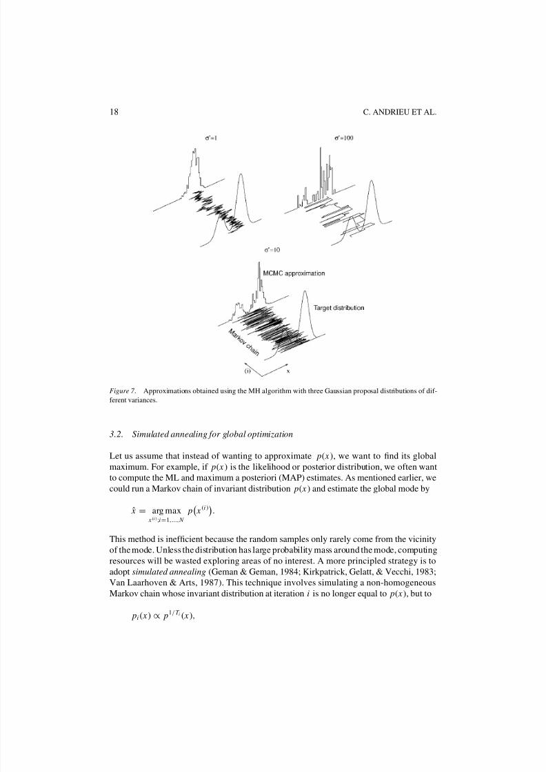
Some properties of the MH algorithm are worth highlighting. Firstly, the normalising

constant of thetarget distribution is notrequired. We only need to know thetarget distributionup to a constant of proportionality. Secondly, although thepseudo-codemakesuse of a single

chain, it is easy to simulate several independent chains in parallel. Lastly, the success or

failure of the algorithm often hingeson the choice of proposal distribution. This is illustrated

in figure 7. Different choices of the proposal standard deviation σ lead to very different

results. If the proposal is too narrow, only one mode of p( x) might be visited. On the other

hand, if it is too wide, the rejection rate can be very high, resulting in high correlations. If all

themodesare visited while theacceptance probability is high, thechainis said to “mix” well.




Figure 7 . Approximations obtained using the MH algorithm with three Gaussian proposal distributions of dif-

ferent variances.

3.2. Simulated annealing for global optimization

Let us assume that instead of wanting to approximate p( x), we want to find its global

maximum. For example, if p( x ) is the likelihood or posterior distribution, we often want

to compute the ML and maximum a posteriori (MAP) estimates. As mentioned earlier, we

could run a Markov chain of invariant distribution p( x ) and estimate the global mode by

ˆ x = arg max x (i );i=1,..., N

p x (i )

.

This method is inef ficient because the random samples only rarely come from the vicinityof the mode. Unless the distribution has large probability mass around the mode, computing

resources will be wasted exploring areas of no interest. A more principled strategy is to

adopt simulated annealing (Geman & Geman, 1984; Kirkpatrick, Gelatt, & Vecchi, 1983;

Van Laarhoven & Arts, 1987). This technique involves simulating a non-homogeneous

Markov chain whose invariant distribution at iteration i is no longer equal to p( x), but to

pi ( x) ∝ p1/T i ( x ),



INTRODUCTION 19

Figure 8. General simulated annealing algorithm.

−10 0 10 200

0.1

0.2

i=100

−10 0 10 200

0.1

0.2

i=500

−10 0 10 200

0.1

0.2

i=1000

−10 0 10 200

0.1

0.2

i=5000

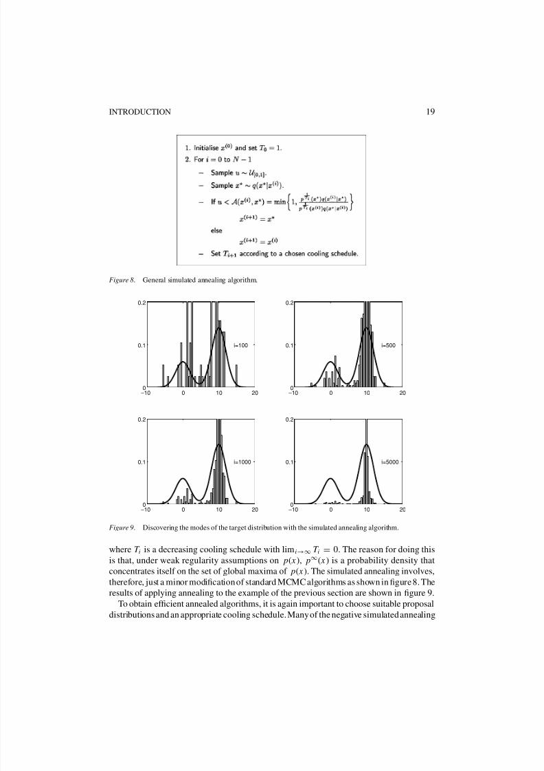
Figure 9. Discovering the modes of the target distribution with the simulated annealing algorithm.

where T i is a decreasing cooling schedule with limi→∞ T i = 0. The reason for doing this

is that, under weak regularity assumptions on p( x), p∞( x ) is a probability density that

concentrates itself on the set of global maxima of p( x). The simulated annealing involves,

therefore, just a minor modification of standard MCMC algorithms as shown in figure 8. The

results of applying annealing to the example of the previous section are shown in figure 9.

To obtain ef ficient annealed algorithms, it is again important to choose suitable proposal

distributions and an appropriate cooling schedule. Many of the negative simulated annealing




results reported in the literature often stem from poor proposal distribution design. In some

complex variable and model selection scenarios arising in machine learning, one can even

propose from complex reversible jump MCMC kernels (Section 3.7) within the annealing

algorithm (Andrieu, de Freitas, & Doucet, 2000a). If one de fines a joint distribution over

the parameter and model spaces, this technique can be used to search for the best model

(according to MDL or AIC criteria) and ML parameter estimates simultaneously.

Most convergence results for simulated annealing typically state that if for a given T i ,

the homogeneous Markov transition kernel mixes quickly enough, then convergence to the

set of global maxima of p( x) is ensured for a sequence T i = (C ln(i + T 0))−1, where C and

T 0 are problem-dependent. Most of the results have been obtained for finite spaces (Geman

& Geman, 1984; Van Laarhoven & Arts, 1987) or compact continuous spaces (Haario &

Sacksman, 1991). Some results for non-compact spaces can be found in Andrieu, Breyer,

and Doucet (1999).

3.3. Mixtures and cycles of MCMC kernels

A very powerful property of MCMC is that it is possible to combine several samplers into

mixtures and cycles of the individual samplers (Tierney, 1994). If the transition kernels K 1and K 2 have invariant distribution p(·) each, then the cycle hybrid kernel K 1 K 2 and the

mixture hybrid kernel ν K 1 + (1 − ν)K 2, for 0 ≤ ν ≤ 1, are also transition kernels with

invariant distribution p(·).

Mixtures of kernels can incorporate global proposals to explore vast regions of the

state space and local proposals to discover finer details of the target distribution (Andrieu,

de Freitas, & Doucet, 2000b; Andrieu & Doucet, 1999; Robert & Casella, 1999). This will

be useful, for example, when the target distribution has many narrow peaks. Here, a globalproposal locks into the peaks while a local proposal allows one to explore the space around

each peak. For example, if we require a high-precision frequency detector, one can use

the fast Fourier transform (FFT) as a global proposal and a random walk as local proposal

(Andrieu & Doucet, 1999). Similarly, in kernel regression and classification, one might want

to have a global proposal that places the bases (kernels) at the locations of the input data and

a local random walk proposal that perturbs these in order to obtain better fits (Andrieu, de

Freitas, & Doucet, 2000b). However, mixtures of kernels also play a big role in many other

samplers, including the reversible jump MCMC algorithm (Section 3.7). The pseudo-code

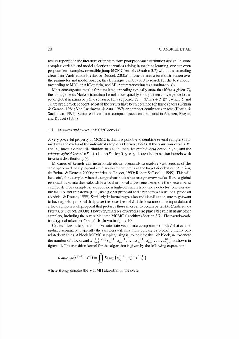
for a typical mixture of kernels is shown in figure 10.

Cycles allow us to split a multivariate state vector into components (blocks) that can be

updated separately. Typically the samplers will mix more quickly by blocking highly cor-

related variables. A block MCMC sampler, using b j to indicate the j -th block, nb to denote

the number of blocks and x(i+1)−[b j ] { x (i+1)

b1, x

(i+1)b2

, . . . , x(i+1)b j−1

, x(i)b j+1

, . . . , x(i )bnb

}, is shown in

figure 11. The transition kernel for this algorithm is given by the following expression

K MH-Cycle

x (i+1)

x (i )

=nb

j=1

K MH(j)

x

(i+1)

b j

x (i )

b j, x

(i+1)−[b j ]

where K MH(j) denotes the j -th MH algorithm in the cycle.



INTRODUCTION 21

Figure 10. Typical mixture of MCMC kernels.

Figure 11. Cycle of MCMC kernels—block MH algorithm.

Obviously, choosing the size of the blocks poses some trade-offs. If one samples the

components of a multi-dimensional vector one-at-a-time, the chain may take a very long

time to explore the target distribution. This problem gets worse as the correlation between

the components increases. Alternatively, if one samples all the components together, then

the probability of accepting this large move tends to be very low.

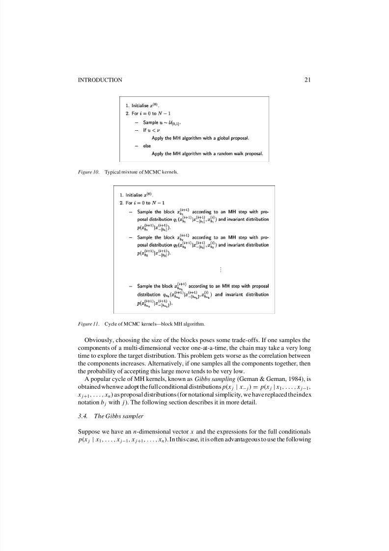
A popular cycle of MH kernels, known as Gibbs sampling (Geman & Geman, 1984), is

obtained whenwe adopt the fullconditional distributions p( x j | x− j ) = p( x j | x1, . . . , x j−1, x j+1, . . . , xn ) as proposal distributions (for notational simplicity, we have replaced theindex

notation b j with j ). The following section describes it in more detail.

3.4. The Gibbs sampler

Suppose we have an n-dimensional vector x and the expressions for the full conditionals

p( x j | x1, . . . , x j−1, x j+1, . . . , xn ). In this case, it is often advantageous to use the following




proposal distribution for j = 1, . . . , n

q x x (i )

=

p x

j

x (i )− j

If x

− j = x(i)− j

0 Otherwise.

The corresponding acceptance probability is:

A x (i ), x

= min

1,

p( x )q x (i )

x

p x (i)

q x | x (i )

= min

1,

p( x ) p x (i)

j x (i )

− j

p x (i)

p( x

j | x − j )

= min

1,

p x

− j

p x

(i)− j

= 1.

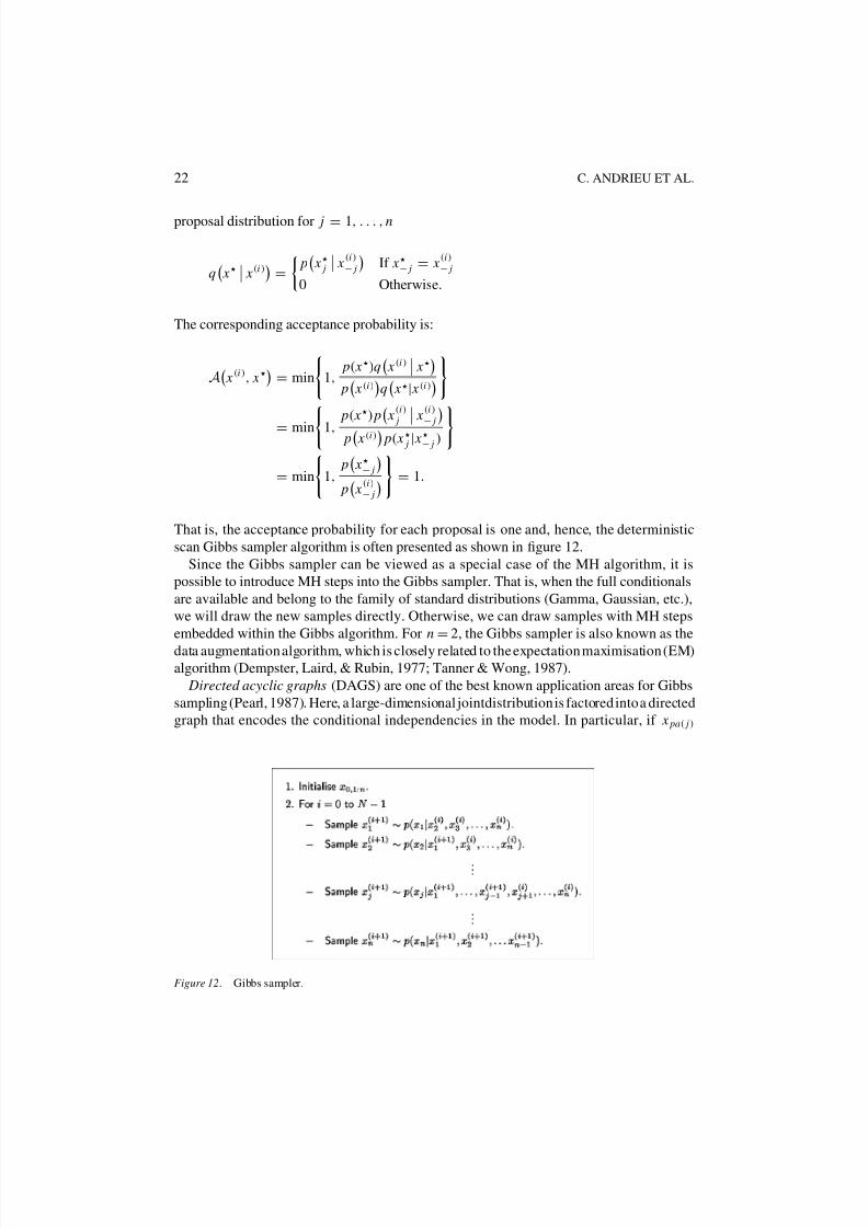
That is, the acceptance probability for each proposal is one and, hence, the deterministic

scan Gibbs sampler algorithm is often presented as shown in figure 12.

Since the Gibbs sampler can be viewed as a special case of the MH algorithm, it is

possible to introduce MH steps into the Gibbs sampler. That is, when the full conditionals

are available and belong to the family of standard distributions (Gamma, Gaussian, etc.),

we will draw the new samples directly. Otherwise, we can draw samples with MH steps

embedded within the Gibbs algorithm. For n

=2, the Gibbs sampler is also known as the

data augmentation algorithm, which is closely related to the expectation maximisation (EM)

algorithm (Dempster, Laird, & Rubin, 1977; Tanner & Wong, 1987).

Directed acyclic graphs (DAGS) are one of the best known application areas for Gibbs

sampling (Pearl, 1987). Here, a large-dimensional jointdistribution is factored into a directed

graph that encodes the conditional independencies in the model. In particular, if x pa( j )

Figure 12. Gibbs sampler.



INTRODUCTION 23

denotes the parent nodes of node x j , we have

p( x) =

j

p x j

x pa( j )

.

It follows that the full conditionals simplify as follows

p x j

x− j

= p

x j

x pa( j )

k ∈ch( j)

p xk

x pa(k )

where ch( j ) denotes the children nodes of x j . That is, we only need to take into account

the parents, the children and the children’s parents. This set of variables is known as the

Markov blanket of x j . This technique forms the basis of the popular software package for

Bayesian updating with Gibbs sampling (BUGS) (Gilks, Thomas, & Spiegelhalter, 1994).

Sampling from the full conditionals, with the Gibbs sampler, lends itself naturally to the

construction of general purpose MCMC software. It is sometimes convenient to block some

of the variables to improve mixing (Jensen, Kong, & Kjærulff, 1995; Wilkinson & Yeung,

2002).

3.5. Monte Carlo EM

The EM algorithm (Baum et al., 1970; Dempster, Laird, & Rubin, 1977) is a standard

algorithm for ML and MAP point estimation. If X contains visible and hidden variables

x = { xv , xh}, then a local maximum of the likelihood p( xv | θ ) given the parameters θ can

be found by iterating the following two steps:

1. E step. Compute the expected value of the complete log-likelihood function with respect

to the distribution of the hidden variables

Q(θ ) = X h

log( p( xh , xv | θ )) p xh

xv, θ (old)

d xh ,

where θ (old) refers to the value of the parameters at the previous time step.

2. M step. Perform the following maximisation θ (new) = arg maxθ Q(θ ).

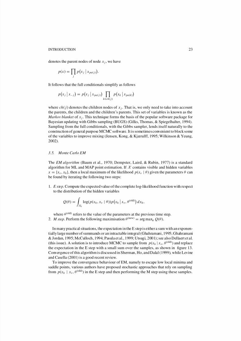
In many practical situations, the expectation in the E step is either a sum with an exponen-

tially large number of summands or an intractable integral (Ghahramani, 1995; Ghahramani

& Jordan, 1995; McCulloch, 1994; Pasula et al., 1999; Utsugi, 2001); see also Dellaert et al.(this issue). A solution is to introduce MCMC to sample from p( xh | xv, θ (old)) and replace

the expectation in the E step with a small sum over the samples, as shown in figure 13.

Convergence of this algorithm is discussed in Sherman, Ho, and Dalal (1999), while Levine

and Casella (2001) is a good recent review.

To improve the convergence behaviour of EM, namely to escape low local minima and

saddle points, various authors have proposed stochastic approaches that rely on sampling

from p( xh | xv , θ (old)) in the E step and then performing the M step using these samples.




Figure 13. MCMC-EM algorithm.

The method is known as stochastic EM (SEM) when we draw only one sample (Celeux

& Diebolt, 1985) and Monte Carlo EM (MCEM) when several samples are drawn (Wei

& Tanner, 1990). There are several annealed variants (such as SAEM) that become more

deterministic as the number of iterations increases (Celeux & Diebolt, 1992). The are also

very ef ficient algorithms for marginal MAPestimation (SAME) (Doucet, Godsill, & Robert,

2000). One wishes sometimes that Metropolis had succeeded in stopping the proliferationof acronyms!

3.6. Auxiliary variable samplers

It is often easier to sample from an augmented distribution p( x , u), where u is an auxiliary

variable, than from p( x). Then, it is possible to obtain marginal samples x (i ) by sampling

( x (i ), u(i )) according to p( x, u) and, subsequently, ignoring the samples u(i ). This very useful

idea was proposed in the physics literature (Swendsen & Wang, 1987). Here, we will focus

on two well-known examples of auxiliary variable methods, namely hybrid Monte Carlo

and slice sampling.

3.6.1. Hybrid Monte Carlo. Hybrid Monte Carlo (HMC) is an MCMC algorithm thatincorporates information about the gradient of the target distribution to improve mixing

in high dimensions. We describe here the “leapfrog” HMC algorithm outlined in Duane

et al. (1987) and Neal (1996) focusing on the algorithmic details and not on the statistical

mechanics motivation. Assume that p( x) is differentiable and everywhere strictly positive.

At each iteration of the HMC algorithm, one takes a predetermined number ( L) of deter-

ministic steps using information about the gradient of p( x). To explain this in more detail,

we first need to introduce a set of auxiliary “momentum” variables u ∈ Rn x and define the



INTRODUCTION 25

Figure 14. Hybrid Monte Carlo.

extended target density

p( x, u) = p( x) N

u; 0, I n x

.

Next, we need to introduce the n x -dimensional gradient vector ( x) ∂ log p( x )/∂ x and

a fixed step-size parameter ρ > 0.

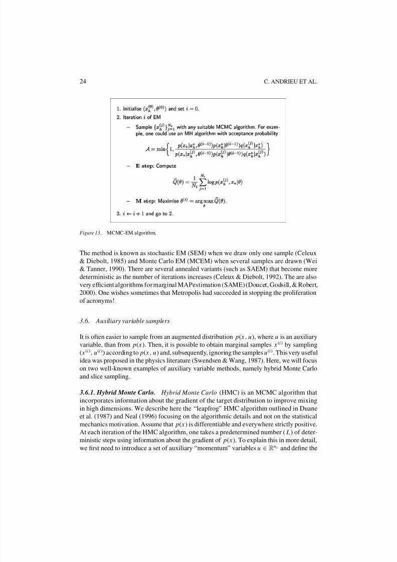
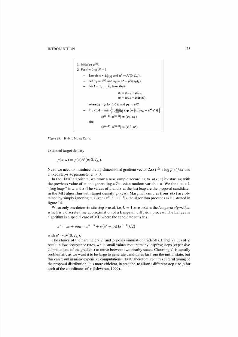
In the HMC algorithm, we draw a new sample according to p( x , u) by starting with

the previous value of x and generating a Gaussian random variable u. We then take L

“frog leaps” in u and x . The values of u and x at the last leap are the proposal candidates

in the MH algorithm with target density p( x, u). Marginal samples from p( x) are ob-

tained by simply ignoring u. Given ( x (i−1), u(i−1)), the algorithm proceeds as illustrated in

figure 14.

When only one deterministic step is used, i.e. L = 1, one obtains the Langevin algorithm,

which is a discrete time approximation of a Langevin diffusion process. The Langevin

algorithm is a special case of MH where the candidate satisfies

x = x0 + ρu0 = x (i−1) + ρ

u + ρ x (i−1)

/2

with u

∼ N (0, I n x ).The choice of the parameters L and ρ poses simulation tradeoffs. Large values of ρ

result in low acceptance rates, while small values require many leapfrog steps (expensive

computations of the gradient) to move between two nearby states. Choosing L is equally

problematic as we want it to be large to generate candidates far from the initial state, but

this can result in many expensive computations. HMC, therefore, requires careful tuning of

the proposal distribution. It is more ef ficient, in practice, to allow a different step size ρ for

each of the coordinates of x (Ishwaran, 1999).




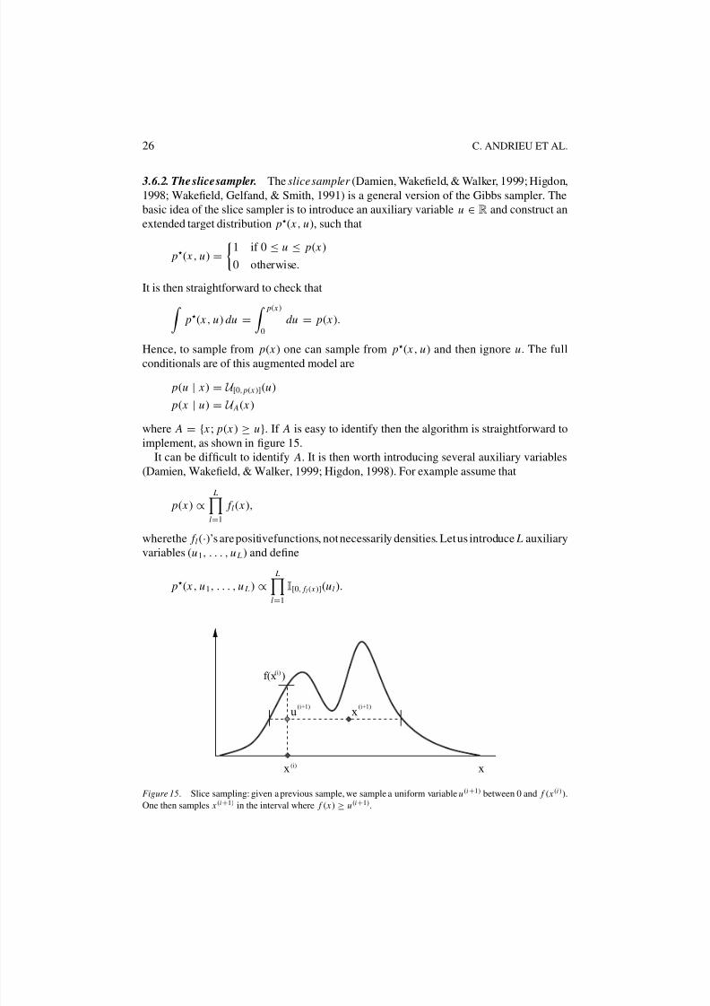
3.6.2. The slice sampler. The slice sampler (Damien, Wakefield, & Walker, 1999; Higdon,

1998; Wakefield, Gelfand, & Smith, 1991) is a general version of the Gibbs sampler. The

basic idea of the slice sampler is to introduce an auxiliary variable u ∈ R and construct an

extended target distribution p( x, u), such that

p( x , u) =

1 if 0 ≤ u ≤ p( x)

0 otherwise.

It is then straightforward to check that p( x , u) du =

p( x)

0

du = p( x).

Hence, to sample from p( x) one can sample from p

( x , u) and then ignore u. The fullconditionals are of this augmented model are

p(u | x) = U [0, p( x )](u)

p( x | u) = U A( x )

where A = { x; p( x ) ≥ u}. If A is easy to identify then the algorithm is straightforward to

implement, as shown in figure 15.

It can be dif ficult to identify A. It is then worth introducing several auxiliary variables

(Damien, Wakefield, & Walker, 1999; Higdon, 1998). For example assume that

p( x) ∝ L

l=1

f l ( x),

wherethe f l (·)’s are positivefunctions, not necessarily densities. Let us introduce L auxiliary

variables (u1, . . . , u L ) and define

p( x , u1, . . . , u L ) ∝ L

l=1

I[0, f l ( x)](ul ).

xx

xu(i+1)

(i)

(i+1)

f(x )(i)

Figure 15. Slice sampling: given a previous sample, we sample a uniform variable u(i+1) between 0 and f ( x (i )).

One then samples x (i+1) in the interval where f ( x) ≥ u(i+1).



INTRODUCTION 27

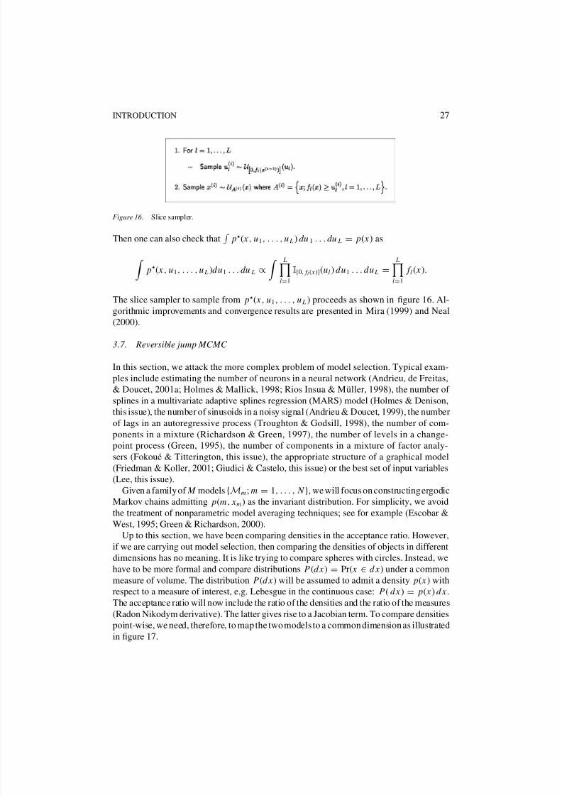
Figure 16 . Slice sampler.

Then one can also check that

p( x, u1, . . . , u L ) du 1 . . . du L = p( x) as

p( x , u1, . . . , u L )du1 . . . du L

∝ L

l=1

I[0, f l ( x )](ul ) du1 . . . du L

=

L

l=1

f l ( x).

The slice sampler to sample from p( x, u1, . . . , u L ) proceeds as shown in figure 16. Al-

gorithmic improvements and convergence results are presented in Mira (1999) and Neal

(2000).

3.7. Reversible jump MCMC

In this section, we attack the more complex problem of model selection. Typical exam-

ples include estimating the number of neurons in a neural network (Andrieu, de Freitas,

& Doucet, 2001a; Holmes & Mallick, 1998; Rios Insua & Muller, 1998), the number of

splines in a multivariate adaptive splines regression (MARS) model (Holmes & Denison,

this issue), the number of sinusoids in a noisy signal (Andrieu & Doucet, 1999), the number

of lags in an autoregressive process (Troughton & Godsill, 1998), the number of com-

ponents in a mixture (Richardson & Green, 1997), the number of levels in a change-

point process (Green, 1995), the number of components in a mixture of factor analy-

sers (Fokoue & Titterington, this issue), the appropriate structure of a graphical model

(Friedman & Koller, 2001; Giudici & Castelo, this issue) or the best set of input variables

(Lee, this issue).

Given a family of M models {Mm ; m = 1, . . . , N }, we will focus on constructing ergodic

Markov chains admitting p(m, xm ) as the invariant distribution. For simplicity, we avoid

the treatment of nonparametric model averaging techniques; see for example (Escobar &

West, 1995; Green & Richardson, 2000).

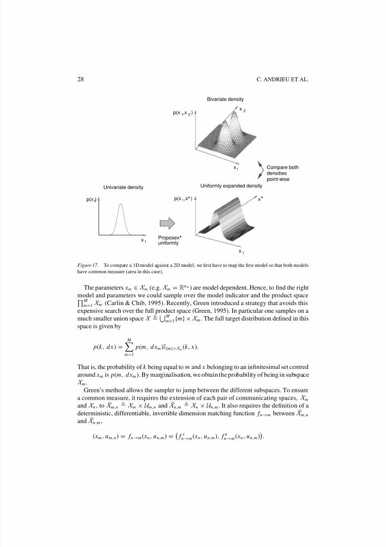
Up to this section, we have been comparing densities in the acceptance ratio. However,

if we are carrying out model selection, then comparing the densities of objects in different

dimensions has no meaning. It is like trying to compare spheres with circles. Instead, wehave to be more formal and compare distributions P(d x) = Pr( x ∈ d x) under a common

measure of volume. The distribution P(d x) will be assumed to admit a density p( x) with

respect to a measure of interest, e.g. Lebesgue in the continuous case: P( d x ) = p( x ) d x .

The acceptance ratio will now include the ratio of the densities and the ratio of the measures

(Radon Nikodym derivative). The latter gives rise to a Jacobian term. To compare densities

point-wise, we need, therefore, to map the two models to a common dimension as illustrated

in figure 17.




1

1

*

*

21

1

Uniformly expanded density

x

Compare bothdensitiespoint-wise

uniformly

*

2

1

Bivariate density

Univariate density

p(x ,x )x

1x

p(x ,x )

Proposexx

p(x ) x

Figure 17 . To compare a 1D model against a 2D model, we first have to map the first model so that both models

have common measure (area in this case).

The parameters xm ∈ X m (e.g. X m = Rnm ) are model dependent. Hence, to find the rightmodel and parameters we could sample over the model indicator and the product space M

m=1 X m (Carlin & Chib, 1995). Recently, Green introduced a strategy that avoids this

expensive search over the full product space (Green, 1995). In particular one samples on a

much smaller union space X M

m=1{m} ×X m . The full target distribution defined in this

space is given by

p(k , d x) = M

m=1

p(m, d xm )I{m}×X m (k , x).

That is, the probability of k being equal to m and x belonging to an infinitesimal set centred

around xm is p(m, d xm ). By marginalisation, we obtain the probability of being in subspace

X m .Green’s method allows the sampler to jump between the different subspaces. To ensure

a common measure, it requires the extension of each pair of communicating spaces, X mand X n , to X m,n X m × U m,n and X n,m X n × U n,m . It also requires the definition of a

deterministic, differentiable, invertible dimension matching function f n→m between X m,n

and X n,m ,

( xm , um,n) = f n→m ( xn, un,m ) =

f xn→m ( xn, un,m ), f u

n→m ( xn , un,m )

.



INTRODUCTION 29

We define f m→n such that f m→n( f n→m ( xn, un,m )) = ( xn , un,m ). The choice of the extended

spaces, deterministic transformation f m→n and proposal distributions for qn→m (· | n, xn)and

qm→n (· | m, xm ) is problem dependent and needs to be addressed on a case by case basis.

If the current state of the chain is (n, xn ), we move to (m, xm ) by generating un,m ∼qn→m (· | n, xn ), ensuring that we have reversibility ( xm , um,n ) = f n→m ( xn , un,m ), and ac-

cepting the move according to the probability ratio

An→m = min

1,

p(m, x m )

p(n, xn)× q(n | m)

q(m | n)× qm→n(um,n | m, x

m )

qn→m (un,m | n, xn)× J f n→m

,

where x m = f x

n→m ( xn, un,m ) and J f n→mis the Jacobian of the transformation f n→m (when

only continuous variables are involved in the transformation)

J f m→n=det

∂ f n→m ( xm , um,n)

∂( xm , um,n)

.To illustrate this, assume that we are concerned with sampling the locations µ and number

k of components of a mixture. For example we might want to estimate the locations and

number of basis functions in kernel regression and classification, the number of mixture

components in a finite mixture model, or the location and number of segments in a segmen-

tation problem. Here, we could define a merge move that combines two nearby components

and a split move that breaks a component into two nearby ones. The merge move involves

randomly selecting a component (µ1) and then combining it with its closest neighbour (µ2)

into a single component µ, whose new location is

µ =µ1

+µ2

2

The corresponding split move that guarantees reversibility, involves splitting a randomly

chosen component as follows

µ1 = µ − un,m β

µ2 = µ + un,m β

where β is a simulation parameter and, for example, un,m ∼ U [0,1]. Note that to ensure

reversibility, we only perform the merge move if µ1 − µ2 < 2β. The acceptance ratio

for the split move is

Asplit = min

1, p(k + 1, µk +1) p(k , µk )

×1

k +11k

× 1 p(un,m )

× J split

,

where 1/k denotes the probability of choosing, uniformly at random, one of the k compo-

nents. The Jacobian is

J split = ∂(µ1, µ2)

∂(µ, un,m )

= 1 1

−β β

= 2β.




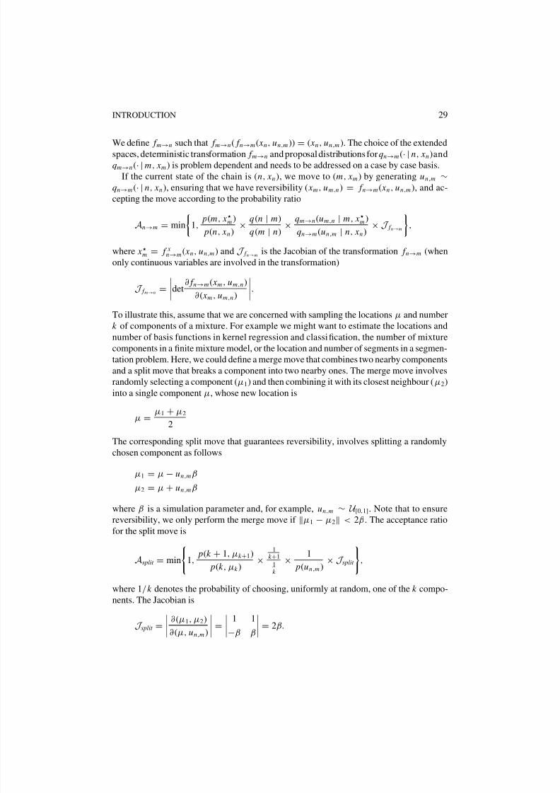
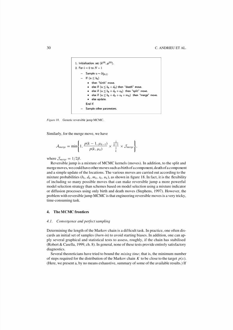
Figure 18. Generic reversible jump MCMC.

Similarly, for the merge move, we have

Amerge = min

1,

p(k − 1, µk −1)

p(k , µk )×

1k −1

1k

× J merge

,

where J merge = 1/2β.

Reversible jump is a mixture of MCMC kernels (moves). In addition, to the split and

merge moves, we could have other moves such as birth of a component, death of a component

and a simple update of the locations. The various moves are carried out according to themixture probabilities (bk , d k , mk , sk , uk ), as shown in figure 18. In fact, it is the flexibility

of including so many possible moves that can make reversible jump a more powerful

model selection strategy than schemes based on model selection using a mixture indicator

or diffusion processes using only birth and death moves (Stephens, 1997). However, the

problem with reversible jump MCMC is that engineering reversible moves is a very tricky,

time-consuming task.

4. The MCMC frontiers

4.1. Convergence and perfect sampling

Determining the length of the Markov chain is a dif ficult task. In practice, one often dis-cards an initial set of samples (burn-in) to avoid starting biases. In addition, one can ap-

ply several graphical and statistical tests to assess, roughly, if the chain has stabilised

(Robert & Casella, 1999, ch. 8). In general, none of these tests provide entirely satisfactory

diagnostics.

Several theoreticians have tried to bound the mixing time; that is, the minimum number

of steps required for the distribution of the Markov chain K to be close to the target p( x).

(Here, we present a, by no means exhaustive, summary of some of the available results.) If



INTRODUCTION 31

we measure closeness with the total variation norm x (t ), where

x (t ) =K (t )(· | x ) − p(·)

= 1

2

K (t )( y | x) − p( y)

d y,

then the mixing time is

τ x () = min{t : x (t ) ≤ for all t ≥ t }.

If the state space X is finite and reversibility holds true, then the transition operator

K (K f ( x ) = K ( y | x) f ( y)) is self adjoint on L2( p). That is,

K f

|g =

f |

K g

,

where f and g are real functions and we have used the bra-ket notation for the inner product

f | g = f ( x)g( x) p( x). This implies that K has real eigenvalues

1 = λ1 > λ2 ≥ λ3 ≥ · · · ≥ λ|X | > −1

and an orthonormal basis of real eigenfunctions f i , such that K f i = λi f i . This spectral

decomposition and the Cauchy-Schwartz inequality allow us to obtain a bound on the total

variation norm

x (t ) ≤ 1

2√

p( x )λt

,

where λ = max(λ2, |λ|X ||) (Diaconis & Saloff-Coste, 1998; Jerrum & Sinclair, 1996). This

classical result give us a geometric convergence rate in terms of eigenvalues. Geometric

bounds have also been obtained in general state spaces using the tools of regeneration and

Lyapunov-Foster conditions (Meyn & Tweedie, 1993).

The next logical step is to bound the second eigenvalue. There are several inequalities

(Cheeger, Poincare, Nash) from differential geometry that allows us to obtain these bounds

(Diaconis & Saloff-Coste, 1998). For example, one could use Cheeger’s inequality to obtain

the following bound

1 − 2 ≤ λ2 ≤ 1 − 2

2,

where is the conductance of the Markov chain

= min0< p(S)<1/2;S⊂X

x∈S, y∈Sc p( x)K ( y | x )

p(S)

Intuitively, one can interpret this quantity as the readiness of the chain to escape from any

small region S of the state space and, hence, make rapid progress towards equilibrium

(Jerrum & Sinclair, 1996).




These mathematical tools have been applied to show that simple MCMC algorithms

(mostly Metropolis) run in time that is polynomial in the dimension d of the state space,

thereby escaping the exponential curse of dimensionality. Polynomial time sampling algo-

rithms have been obtained in the following important scenarios:

1. Computing the volume of a convex body in d dimensions, where d is large (Dyer, Frieze,

& Kannan, 1991).

2. Sampling from log-concave distributions (Applegate & Kannan, 1991).

3. Sampling from truncated multivariate Gaussians (Kannan & Li, 1996).

4. Computing the permanent of a matrix (Jerrum, Sinclair, & Vigoda, 2000).

The last problem is equivalent to sampling matchings from a bipartite graph; a problem

that manifests itself in many ways in machine learning (e.g., stereo matching and dataassociation).

Although the theoretical results are still far from the practice of MCMC, they will even-

tually provide better guidelines on how to design and choose algorithms. Already, some

results tell us, for example, that it is not wise to use the independent Metropolis sampler in

high dimensions (Mengersen & Tweedie, 1996).

A remarkable recent breakthrough was the development of algorithms for perfect sam-

pling. These algorithms are guaranteed to give us an independent sample from p( x ) under

certain restrictions. The two major players are coupling from the past (Propp & Wilson,

1998) and Fill’s algorithm (Fill, 1998). From a practical point of view, these algorithms are

still limited and, in many cases, computationally inef ficient. However, some steps are being

taken towards obtaining more general perfect samplers; for example perfect slice samplers

(Casella et al., 1999).

4.2. Adaptive MCMC

If we look at the chain on the top right of figure 7, we notice that the chain stays at each state

for a long time. This tells us that we should reduce the variance of the proposal distribution.

Ideally, onewould like to automate this process of choosing theproposaldistribution asmuch

as possible.That is,one shoulduse theinformationin thesamples to updatethe parameters of

the proposal distribution so as to obtain a distribution that is either closer to the target distri-

bution, that ensures a suitable acceptance rate, or that minimisesthe varianceof theestimator

of interest. However, one should not allow adaptation to take place infinitely often in a naive

way because this can disturb the stationarydistribution.This problem arises because by using

the past information infinitely often, we violate the Markov property of the transition kernel.That is, p( x (i) | x (0), x (1), . . . , x (i−1)) no longer simplifies to p( x (i ) | x (i−1)). In particular,

Gelfand andSahu (1994)present a pathologicalexample,where thestationary distribution is

disturbed despite the fact that each participating kernel has the same stationary distribution.

To avoid this problem, one could carry out adaptation only during an initial fixed number

of steps,and then usestandard MCMC simulation to ensureconvergenceto therightdistribu-

tion. Two methods for doing this are presented in Gelfand and Sahu (1994). Thefirst is based

on the idea of running several chains in parallel and using sampling-importance resampling



INTRODUCTION 33

(Rubin, 1988) to multiply the kernels that are doing well and suppress the others. In this

approach, one uses an approximation to the marginal density of the chain as proposal. The

secondmethod simplyinvolves monitoring thetransition kernel andchangingone of itscom-

ponents (for example the proposal distribution) so as to improve mixing. A similar method

that guarantees a particular acceptance rate is discussed in Browne and Draper (2000).

There are, however, a few adaptive MCMC methods that allow one to perform adaptation

continuously without disturbing the Markov property, including delayed rejection (Tierney

& Mira, 1999), parallel chains (Gilks & Roberts, 1996) and regeneration (Gilks, Roberts, &

Sahu, 1998; Mykland, Tierney, & Yu, 1995). These methods are, unfortunately, inef ficient

in many ways and much more research is required in this exciting area.

4.3. Sequential Monte Carlo and particle filters

Sequential Monte Carlo (SMC) methods allow us to carry out on-line approximation of

probability distributions using samples (particles). They are very useful in scenarios involv-

ing real-time signal processing, where data arrival is inherently sequential. Furthermore,

one might wish to adopt a sequential processing strategy to deal with non-stationarity in

signals, so that information from the recent past is given greater weighting than information

from the distant past. Computational simplicity in the form of not having to store all the

data might also constitute an additional motivating factor for these methods.

In the SMC setting, we assume that we have an initial distribution, a dynamic model and

measurement model

p( x0)

p( xt | x0:t −1, y1:t −1) for t ≥ 1 p( yt | x0:t , y1:t −1) for t ≥ 1

We denote by x0:t { x0, . . . , xt } and y1:t { y1, . . . , yt }, respectively, the states and the ob-

servations up to time t . Note that we could assume Markov transitions and conditional inde-

pendence to simplify the model; p( xt | x0:t −1, y1:t −1) = p( xt | xt −1) and p( yt | x0:t , y1:t −1) = p( yt | xt ). However, this assumption is not necessary in the SMC framework.

Our aim is to estimate recursively in time the posterior p( x0:t | y1:t ) and its associated

features including the marginal distribution p( xt | y1:t ), known as the filtering distribution,

and the expectations

I ( f t ) = E p( x0:t | y1:t ) [ f t ( x0:t )]

A generic SMC algorithm is depicted in figure 19. Given N particles { x (i )0:t −1} N

i=1 at

time t − 1, approximately distributed according to the distribution p( x0:t −1 | y1:t −1), SMC

methods allow us to compute N particles { x (i )0:t } N

i=1 approximately distributed according to

the posterior p( x0:t | y1:t ), at time t . Since we cannot sample from the posterior directly,

the SMC update is accomplished by introducing an appropriate importance proposal dis-

tribution q( x0:t ) from which we can obtain samples. The samples are then appropriately

weighted.




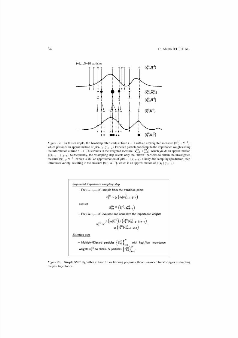
Figure 19. In this example, the bootstrap filter starts at time t − 1 with an unweighted measure {x(i )t −1, N −1},

which provides an approximation of p(xt −1 | y1:t −2). For each particle we compute the importance weights using

the information at time t − 1. This results in the weighted measure {x(i )t −1, w

(i )t −1

}, which yields an approximation

p(xt −1 | y1:t −1). Subsequently, the resampling step selects only the “fittest” particles to obtain the unweighted

measure {x(i )t −1, N −1}, which is still an approximation of p(xt −1 | y1:t −1). Finally, the sampling (prediction) step

introduces variety, resulting in the measure {x(i )t , N −1}, which is an approximation of p(xt | y1:t −1).

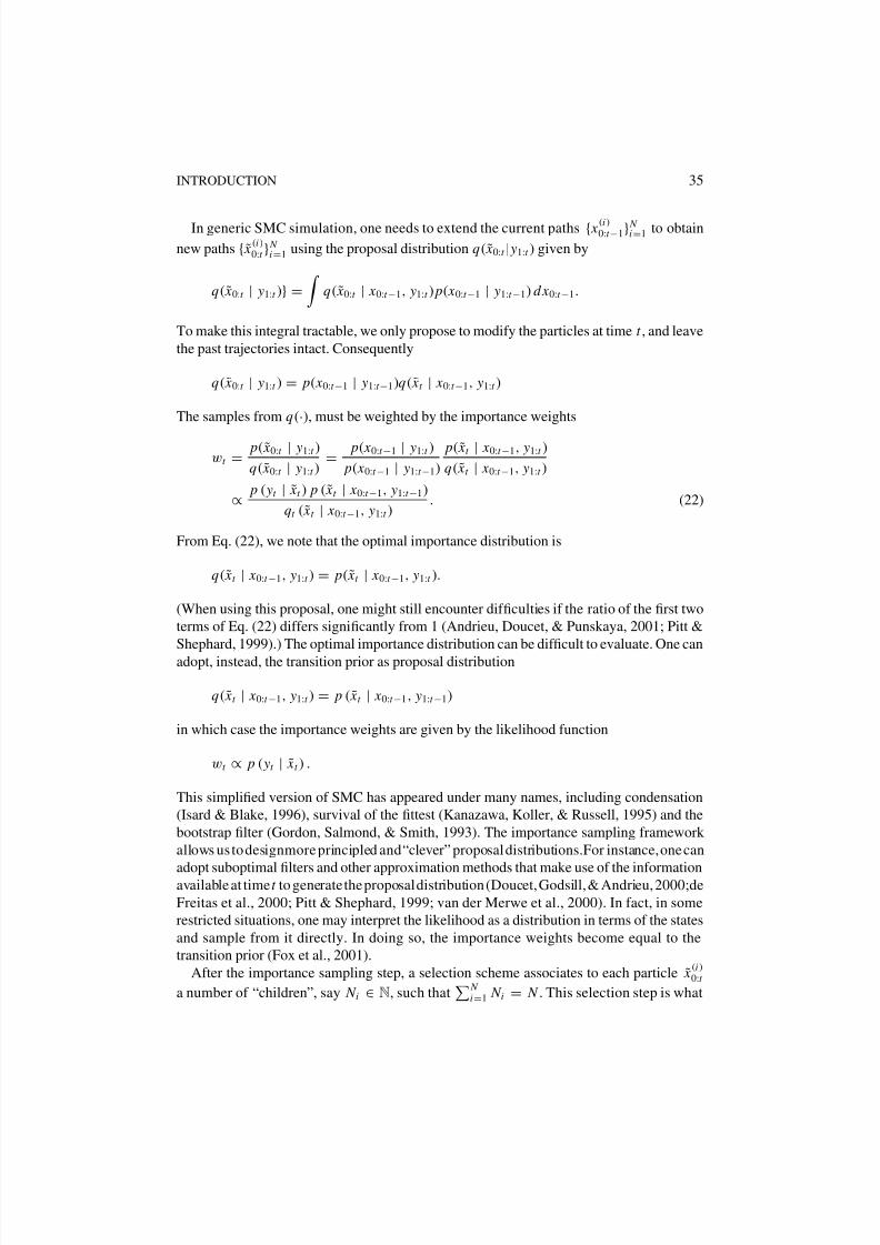
Figure 20. Simple SMC algorithm at time t . For filtering purposes, there is no need for storing or resampling

the past trajectories.



INTRODUCTION 35

In generic SMC simulation, one needs to extend the current paths { x (i )0:t −1} N

i=1 to obtain

new paths { ˜ x(i )0:t } N

i=1 using the proposal distribution q( ˜ x0:t | y1:t ) given by

q( ˜ x0:t | y1:t )} =

q( ˜ x0:t | x0:t −1, y1:t ) p( x0:t −1 | y1:t −1) d x0:t −1.

To make this integral tractable, we only propose to modify the particles at time t , and leave

the past trajectories intact. Consequently

q( ˜ x0:t | y1:t ) = p( x0:t −1 | y1:t −1)q( ˜ xt | x0:t −1, y1:t )

The samples from q(·), must be weighted by the importance weights

wt = p( ˜ x0:t | y1:t )

q( ˜ x0:t | y1:t )= p( x0:t −1 | y1:t )

p( x0:t −1 | y1:t −1)

p( ˜ xt | x0:t −1, y1:t )

q( ˜ xt | x0:t −1, y1:t )

∝ p ( yt | ˜ xt ) p ( ˜ xt | x0:t −1, y1:t −1)

qt ( ˜ xt | x0:t −1, y1:t ). (22)

From Eq. (22), we note that the optimal importance distribution is

q( ˜ xt | x0:t −1, y1:t ) = p( ˜ xt | x0:t −1, y1:t ).

(When using this proposal, one might still encounter dif ficulties if the ratio of the first two

terms of Eq. (22) differs significantly from 1 (Andrieu, Doucet, & Punskaya, 2001; Pitt &

Shephard, 1999).) The optimal importance distribution can be dif ficult to evaluate. One can

adopt, instead, the transition prior as proposal distribution

q( ˜ xt | x0:t −1, y1:t ) = p ( ˜ xt | x0:t −1, y1:t −1)

in which case the importance weights are given by the likelihood function

wt ∝ p ( yt | ˜ xt ) .

This simplified version of SMC has appeared under many names, including condensation

(Isard & Blake, 1996), survival of the fittest (Kanazawa, Koller, & Russell, 1995) and the

bootstrap filter (Gordon, Salmond, & Smith, 1993). The importance sampling framework

allows us to designmore principled and“clever” proposal distributions.For instance, one can

adopt suboptimal filters and other approximation methods that make use of the informationavailable at time t to generate the proposaldistribution (Doucet, Godsill, & Andrieu, 2000;de

Freitas et al., 2000; Pitt & Shephard, 1999; van der Merwe et al., 2000). In fact, in some

restricted situations, one may interpret the likelihood as a distribution in terms of the states

and sample from it directly. In doing so, the importance weights become equal to the

transition prior (Fox et al., 2001).

After the importance sampling step, a selection scheme associates to each particle ˜ x(i )0:t

a number of “children”, say N i ∈ N, such that N

i=1 N i = N . This selection step is what




allows us to track moving target distributions ef ficiently by choosing the fittest particles.

There are various selection schemes in the literature, but their performance varies in terms

of var [ N i ] (Doucet, de Freitas, & Gordon, 2001).

An important feature of the selection routine is that its interface only depends on particle

indices and weights. That is, it can be treated as a black-box routine that does not require

any knowledge of what a particle represents (e.g., variables, parameters, models). This

enables one to implement variable and model selection schemes straightforwardly. The

simplicity of the coding of complex models is, indeed, one of the major advantages of these

algorithms.

It is also possible to introduce MCMC steps of invariant distribution p( x0:t | y1:t ) on each

particle (Andrieu, de Freitas, & Doucet, 1999; Gilks & Berzuini, 1998; MacEachern, Clyde,

& Liu, 1999). The basic idea is that if the particles are distributed according to the poste-

rior distribution p( x0:t | y1:t ), then applying a Markov chain transition kernel K ( x0:t | x0:t ),

with invariant distribution p(· | y1:t ) such that

K ( x 0:t | x0:t ) p( x0:t | y1:t ) = p( x

0:t | y1:t ), still

results in a set of particles distributed according to the posterior of interest. However, the

new particles might have been moved to more interesting areas of the state-space. In fact,

by applying a Markov transition kernel, the total variation of the current distribution with

respect to the invariant distribution can only decrease. Note that we can incorporate any

of the standard MCMC methods, such as the Gibbs sampler, MH algorithm and reversible

jump MCMC, into the filtering framework, but we no longer require the kernel to be

ergodic.

4.4. The machine learning frontier

The machine learning frontier is characterised by large dimensional models, massive datasetsand many and varied applications. Massive datasets pose no problem in the SMC context.

However, in batch MCMC simulation it is often not possible to load the entire dataset

into memory. A few solutions based on importance sampling have been proposed recently

(Ridgeway, 1999), but there is still great room for innovation in this area.

Despite the auspicious polynomial bounds on the mixing time, it is an arduous task

to design ef ficient samplers in high dimensions. The combination of sampling algorithms

with either gradient optimisation or exact methods has proved to be very useful. Gradient

optimisation is inherent to Langevin algorithms and hybrid Monte Carlo. These algorithms

have been shown to work with large dimensional models such as neural networks (Neal,

1996) and Gaussian processes (Barber & Williams, 1997). Information about derivatives of

the target distribution also forms an integral part of many adaptive schemes, as discussed

in Section 2.3. Recently, it has been argued that the combination of MCMC and variationaloptimisation techniques can also lead to more ef ficient sampling (de Freitas et al., 2001).

The combination of exact inference with sampling methods within the framework of Rao-

Blackwellisation (Casella & Robert, 1996) can also result in great improvements. Suppose

we candivide the hidden variables x into twogroups, u and v, such that p( x) = p(v | u) p(u)

and, conditional on u, the conditional posterior distribution p(v | u) is analytically tractable.

Then we can easily marginalise out v from the posterior, and only need to focus on sampling

from p(u), which lies in a space of reduced dimension. That is, we sample u(i ) ∼ p(u) and



INTRODUCTION 37

then use exact inference to compute

p(v) = 1

N

N i=1

p

v u(i )

By identifying “troublesome” variables and sampling them, the rest of the problem can

often be solved easily using exact algorithms such as Kalman filters, HMMs or junction

trees. For example, one can apply this technique to sample variables that eliminate loops in

graphical models and then compute the remaining variables with ef ficient analytical algo-

rithms (Jensen, Kong, & Kjærulff, 1995;Wilkinson & Yeung, 2002). Other application areas

include dynamic Bayesian networks (Doucet et al., 2000), conditionally Gaussian models

(Carter & Kohn, 1994; De Jong & Shephard, 1995; Doucet, 1998) and model averaging

for graphical models (Friedman & Koller, this issue). The problem of how to automatically

identify which variables should be sampled, and which can be handled analytically is still

open. An interesting development is the augmentation of high dimensional models with

low dimensional artificial variables. By sampling only the artificial variables, the original

model decouples into simpler, more tractable submodels (Albert & Chib, 1993; Andrieu, de

Freitas, & Doucet, 2001b; Wood & Kohn, 1998); see also Holmes and Denison (this issue).

This strategy allows one to map probabilistic classification problems to simpler regression

problems.

The design of ef ficient sampling methods most of the times hinges on awareness of

the basic building blocks of MCMC (mixtures of kernels, augmentation strategies and

blocking) and on careful design of the proposal mechanisms. The latter requires domain

specific knowledge and heuristics. There are great opportunities for combining existing

sub-optimal algorithms with MCMC in many machine learning problems. Some areas thatare already benefiting from sampling methods include:

1. Computer vision. Tracking (Isard & Blake, 1996; Ormoneit, Lemieux, & Fleet, 2001),

stereo matching (Dellaertet al., this issue), colour constancy (Forsyth, 1999), restoration

of oldmovies (Morris, Fitzgerald, & Kokaram,1996)and segmentation (Clark& Quinn,

1999; Kam, 2000; Tu & Zhu, 2001).

2. Web statistics. Estimating coverage of search engines, proportions belonging to specific

domains and the average size of web pages (Bar-Yossef et al., 2000).

3. Speech and audio processing. Signal enhancement (Godsill & Rayner, 1998; Vermaak

et al., 1999).

4. Probabilistic graphical models. For example (Gilks, Thomas, & Spiegelhalter, 1994;

Wilkinson & Yeung, 2002) and several papers in this issue.5. Regression and classi fication. Neural networks and kernel machines (Andrieu, de

Freitas, & Doucet, 2001a; Holmes & Mallick, 1998; Neal, 1996; Muller & Rios

Insua, 1998), Gaussian processes (Barber & Williams, 1997), CART (Denison, Mallick,

& Smith, 1998) and MARS (Holmes & Denison, this issue).

6. Computer graphics. Light transport (Veach & Guibas, 1997) and sampling plausible

solutions to multi-body constraint problems (Chenney & Forsyth, 2000).




7. Data association. Vehicle matching in highway systems (Pasula et al., 1999) and mul-

titarget tracking (Bergman, 1999).

8. Decision theory. Partially observable Markov decision Processes (POMDPs) (Thrun,

2000; Salmond & Gordon, 2001), abstract Markov policies (Bui, Venkatesh, & West,

1999) and influence diagrams (Bielza, Muller, & Rios Insua, 1999).

9. First order probabilistic logic. (Pasula & Russell, 2001).

10. Genetics and molecular biology. DNA microarray data (West et al., 2001), cancer gene

mapping (Newton & Lee, 2000), protein alignment (Neuwald et al., 1997) and linkage

analysis (Jensen, Kong, & Kjærulff, 1995).

11. Robotics. Robot localisation and map building (Fox et al., 2001).

12. Classical mixture models. Mixtures of independent factor analysers (Utsugi, 2001) and

mixtures of factor analysers (Fokoue & Titterington, this issue).

We hope that this review will be a useful resource to people wishing to carry out further

research at the interface between MCMC and machine learning. For conciseness, we have

skipped many interesting ideas, including tempering and coupling. For more details, we

advise the readers to consult the references at the end of this paper.

Acknowledgments

We would like to thank Robin Morris, Kevin Murphy, Mark Paskin, Sekhar Tatikonda and

Mike Titterington.

References

Al-Qaq, W. A., Devetsikiotis, M., & Townsend, J. K. (1995). Stochastic gradient optimization of importance sam-

pling for the ef ficient simulation of digital communication systems. IEEE Transactions on Communications,

43:12, 2975–2985.

Albert, J., & Chib, S. (1993). Bayesian analysis of binary and polychotomous response data. Journal of the

American Statistical Association, 88:422, 669–679.

Anderson, H. L. (1986). Metropolis, Monte Carlo, and the MANIAC. Los Alamos Science, 14, 96–108.

Andrieu, C., & Doucet, A. (1999). Joint Bayesian detection and estimation of noisy sinusoids via reversible jump

MCMC. IEEE Transactions on Signal Processing, 47:10, 2667–2676.

Andrieu, C., Breyer, L. A., & Doucet, A. (1999). Convergence of simulated annealing using Foster-Lyapunov

criteria. Technical Report CUED/F-INFENG/TR 346, Cambridge University Engineering Department.

Andrieu, C.,de Freitas, N.,& Doucet, A. (1999).Sequential MCMC forBayesian model selection.In IEEE Higher

Order Statistics Workshop, Caesarea, Israel (pp. 130–134).

Andrieu, C., de Freitas, N., & Doucet, A. (2000a). Reversible jump MCMC simulated annealing for neural

networks. In Uncertainty in arti ficial intelligence (pp. 11–18). San Mateo, CA: Morgan Kaufmann.

Andrieu, C., de Freitas, N., & Doucet, A. (2000b). Robust full Bayesian methods for neural networks. In S. A.

Solla,T.K. Leen, & K.-R. Muller(Eds.), Advances in neuralinformation processingsystems 12 (pp. 379–385).

MIT Press.

Andrieu, C., de Freitas, N., & Doucet, A. (2001a). Robust full Bayesian learning for radial basis networks. Neural

Computation, 13:10, 2359–2407.

Andrieu, C., de Freitas, N., & Doucet, A. (2001b). Rao-blackwellised particle filtering via data augmentation.

Advances in Neural Information Processing Systems ( NIPS13).



INTRODUCTION 39

Andrieu, C., Doucet, A., & Punskaya, E. (2001). Sequential Monte Carlo methods for optimal filtering. In A

Doucet, N. de Freitas, & N. J. Gordon (Eds.), Sequential Monte Carlo methods in practice. Berlin: Springer-

Verlag.

Applegate, D., & Kannan, R. (1991). Sampling and integration of near log-concave functions. In Proceedings of

the Twenty Third Annual ACM Symposium on Theory of Computing (pp. 156–163).

Bar-Yossef, Z., Berg, A., Chien, S., Fakcharoenphol, J., & Weitz, D. (2000). Approximating aggregate queries

about web pages via random walks. In International Conference on Very Large Databases (pp. 535–544).

Barber, D., & Williams, C. K. I. (1997). Gaussian processes for Bayesian classification via hybrid Monte Carlo.

In M. C. Mozer, M. I. Jordan, & T. Petsche (Eds.), Advances in neural information processing systems 9

(pp. 340–346). Cambridge, MA: MIT Press.

Baum, L. E., Petrie, T., Soules, G., & Weiss, N. (1970). A maximization technique occurring in the statistical

analysis of probabilistic functions of Markov chains. Annals of Mathematical Statistics, 41, 164–171.

Baxter, R. J. (1982). Exactly solved models in statistical mechanics. San Diego, CA: Academic Press.

Beichl, I., & Sullivan, F. (2000). The Metropolis algorithm. Computing in Science & Engineering, 2:1, 65–69.

Bergman, N. (1999). Recursive Bayesian estimation: Navigation and tracking applications. Ph.D. Thesis, Depart-

ment of Electrical Engineering, Link oping University, Sweden.

Berners-Lee, T., Cailliau, R., Luotonen, A., Nielsen, H. F., & Secret, A. (1994). The World-Wide Web. Commu-

nications of the ACM, 10:4, 49–63.

Besag, J., Green, P. J., Hidgon, D., & Mengersen, K. (1995). Bayesian computation and stochastic systems.

Statistical Science, 10:1, 3–66.

Bielza, C., Muller, P., & Rios Insua, D. (1999). Decision Analysis by Augmented Probability Simulation,

Management Science, 45:7 , 995–1007.

Brooks, S. P. (1998). Markov chain Monte Carlo method and its application. The Statistician, 47:1, 69–100.

Browne, W. J., & Draper, D. (2000). Implementation and performance issuesin the Bayesian and likelihood fitting

of multilevel models. Computational Statistics, 15, 391–420.

Bucher, C. G. (1988).Adaptive sampling—An iterative fast Monte Carlo procedure. Structural Safety, 5,119–126.

Bui, H. H., Venkatesh, S., & West, G. (1999). On the recognition of abstract Markov policies. In National

Conference on Arti ficial Intelligence (AAAI-2000).

Carlin, B. P., & Chib, S. (1995).BayesianModel choice viaMCMC. Journal of theRoyal Statistical SocietySeries

B, 57 , 473–484.Carter, C. K., & Kohn, R. (1994). On Gibbs sampling for state space models. Biometrika, 81:3, 541–553.

Casella, G., & Robert, C. P. (1996). Rao-Blackwellisation of sampling schemes. Biometrika, 83:1, 81–94.

Casella, G., Mengersen, K. L., Robert, C. P., & Titterington, D. M. (1999). Perfect slice samplers for mixtures of

distributions. Technical Report BU-1453-M, Department of Biometrics, Cornell University.

Celeux, G., & Diebolt, J. (1985). The SEM algorithm: A probabilistic teacher algorithm derived from the EM

algorithm for the mixture problem. Computational Statistics Quarterly, 2, 73–82.

Celeux, G.,& Diebolt, J. (1992). A stochastic approximation type EM algorithmfor themixture problem. Stochas-

tics and Stochastics Reports, 41, 127–146.

Chen, M.H., Shao, Q.M., & Ibrahim, J.G. (Eds.) (2001). Monte Carlo methodsfor Bayesian computation. Berlin:

Springer-Verlag.

Cheng,J., & Druzdzel,M. J. (2000).AIS-BN: An adaptiveimportance sampling algorithm forevidential reasoning

in large bayesian networks. Journal of Arti ficial Intelligence Research, 13, 155–188.

Chenney,S., & Forsyth, D. A. (2000).Samplingplausiblesolutionsto multi-body constraintproblems. SIGGRAPH

(pp. 219–228).

Clark, E., & Quinn, A. (1999). A data-driven Bayesian sampling scheme for unsupervised image segmentation.In IEEE International Conference on Acoustics, Speech, and Signal Processing , Arizona (Vol. 6, pp. 3497–

3500).

Damien, P., Wakefield, J., & Walker, S. (1999). Gibbs sampling for Bayesian non-conjugate and hierarchical

models by auxiliary variables. Journal of the Royal Statistical Society B , 61:2, 331–344.

de Freitas, N., Hø jen-Sørensen, P., Jordan, M. I., & Russell, S. (2001). Variational MCMC. In J. Breese & D.

Koller (Eds.), Uncertainty in arti ficial intelligence (pp. 120–127). San Matio, CA: Morgan Kaufmann.

de Freitas, N., Niranjan, M., Gee, A. H., & Doucet, A. (2000). Sequential Monte Carlo methods to train neural

network models. Neural Computation, 12:4, 955–993.




De Jong, P., & Shephard, N. (1995). Ef ficient sampling from the smoothing density in time series models.

Biometrika, 82:2, 339–350.

Dempster, A. P., Laird, N. M., & Rubin, D. B. (1997). Maximum likelihood from incomplete data via the EM

algorithm. Journal of the Royal Statistical Society Series B , 39, 1–38.

Denison, D. G. T., Mallick, B. K., & Smith, A. F. M. (1998). A Bayesian CART algorithm. Biometrika, 85,

363–377.

Diaconis, P., & Saloff-Coste, L. (1998). What do we know about the Metropolis algorithm? Journal of Computer

and System Sciences, 57 , 20–36.

Doucet, A. (1998). On sequential simulation-based methods for Bayesian filtering. Technical Report CUED/F-

INFENG/TR 310, Department of Engineering, Cambridge University.

Doucet, A., de Freitas, N., & Gordon, N. J. (Eds.) (2001). Sequential Monte Carlo methods in practice. Berlin:

Springer-Verlag.

Doucet, A., de Freitas, N., Murphy, K., & Russell, S. (2000). Rao blackwellised particle filtering for dynamic

Bayesian networks.In C. Boutilier & M. Godszmidt(Eds.), Uncertaintyin arti ficial intelligence (pp. 176–183).

Morgan Kaufmann Publishers.

Doucet, A.,Godsill,S., & Andrieu, C. (2000).On sequential Monte Carlo sampling methodsfor Bayesian filtering.

Statistics and Computing, 10:3, 197–208.

Doucet, A., Godsill, S. J., & Robert, C. P. (2000). Marginal maximum a posteriori estimation using MCMC.

Technical Report CUED/F-INFENG/TR 375, Cambridge University Engineering Department.

Duane, S., Kennedy, A. D., Pendleton, B. J., & Roweth, D. (1987). Hybrid Monte Carlo. Physics Letters B , 195:2,

216–222.

Dyer, M., Frieze, A., & Kannan, R. (1991). A random polynomial-time algorithm for approximating the volume

of convex bodies. Journal of the ACM, 1:38, 1–17.

Eckhard, R. (1987). Stan Ulam, John Von Neumann and the Monte Carlo method. Los Alamos Science, 15,

131–136.

Escobar, M. D., & West, M. (1995). Bayesian density estimation and inference using mixtures. Journal of the

American Statistical Association, 90, 577–588.

Fill, J. A. (1998). An interruptible algorithm for perfect sampling via Markov chains. The Annals of Applied

Probability, 8 :1, 131–162.

Forsyth, D. A. (1999). Sampling, resampling and colour constancy. In IEEE Conference on Computer Vision and Pattern Recognition (pp. 300–305).

Fox, D., Thrun, S., Burgard, W., & Dellaert, F. (2001). Particle filters for mobile robot localization. In A. Doucet,

N. de Freitas, & N. J. Gordon (Eds.), Sequential Monte Carlo methods in practice. Berlin: Springer-Verlag.

Gelfand, A. E., & Sahu, S. K. (1994). On Markov chain Monte Carlo acceleration. Journal of Computational and

Graphical Statistics, 3, 261–276.

Gelfand, A. E., & Smith, A. F. M. (1990). Sampling-based approaches to calculating marginal densities. Journal

of the American Statistical Association, 85:410, 398–409.

Geman,S., & Geman,D. (1984).Stochastic relaxation, Gibbs distributions andthe Bayesian restoration of images.

IEEE Transactions on Pattern Analysis and Machine Intelligence, 6:6 , 721–741.

Geweke, J. (1989). Bayesian inference in econometric models using Monte Carlo integration. Econometrica, 24,

1317–1399.

Ghahramani, Z. (1995). Factorial learning and the EM algorithm. In G. Tesauro, D. S. Touretzky, & J. Alspector

(Eds.), Advances in neural information processing systems 7 (pp. 617–624).

Ghahramani, Z., & Jordan, M. (1995). Factorial hidden Markov models. Technical Report 9502, MIT Artificial

Intelligence Lab, MA.Gilks, W. R., & Berzuini, C. (1998). Monte Carlo inference for dynamic Bayesian models. Unpublished. Medical

Research Council, Cambridge, UK.

Gilks, W. R., & Roberts, G. O. (1996). Strategies for improving MCMC. In W. R. Gilks, S. Richardson, & D. J.

Spiegelhalter (Eds.), Markov chain Monte Carlo in practice (pp. 89–114). Chapman & Hall.

Gilks, W. R., Richardson, S., & Spiegelhalter, D. J. (Eds.) (1996). Markov chain Monte Carlo in practice. Suffolk:

Chapman and Hall.

Gilks, W. R., Roberts, G. O., & Sahu, S. K. (1998). Adaptive Markov chain Monte Carlo through regeneration.

Journal of the American Statistical Association, 93, 763–769.



INTRODUCTION 41

Gilks,W. R., Thomas, A.,& Spiegelhalter,D. J. (1994).A language andprogram for complex Bayesian modelling.

The Statistician, 43, 169–178.

Godsill, S. J., & Rayner, P. J. W. (Eds.) (1998). Digital audio restoration: A statistical model based approach.

Berlin: Springer-Verlag.

Gordon, N. J., Salmond, D. J., & Smith, A. F. M. (1993). Novel approach to nonlinear/non-Gaussian Bayesian

state estimation. IEE Proceedings-F, 140:2, 107–113.

Green, P. J. (1995). Reversible jump Markov chain Monte Carlo computation and Bayesian model determination.

Biometrika, 82, 711–732.

Green,P.J., & Richardson, S. (2000).Modellingheterogeneity with andwithout theDirichlet process. Department

of Statistics, Bristol University.

Haario, H., & Sacksman, E. (1991). Simulated annealing process in general state space. Advances in Applied

Probability, 2 3, 866–893.

Hastings, W. K. (1970). Monte Carlo sampling methods using Markov chains and their Applications. Biometrika

57 , 97–109.

Higdon, D. M. (1998). Auxiliary variable methods for Markov chain Monte Carlo with application. Journal of


Holmes, C. C., & Mallick, B. K. (1998). Bayesian radial basis functions of variable dimension. Neural Compu-

tation, 10:5, 1217–1233.

Isard, M., & Blake, A. (1996). Contour tracking by stochastic propagation of conditional density. In European

Conference on Computer Vision (pp. 343–356). Cambridge, UK.

Ishwaran, H. (1999). Application of hybrid Monte Carlo to Bayesian generalized linear models: Quasicomplete

separation and neural networks. Journal of Computational and Graphical Statistics, 8, 779–799.

Jensen, C.S.,Kong,A.,& Kjærulff, U. (1995).Blocking-Gibbssampling in very large probabilistic expert systems.

International Journal of Human-Computer Studies, 42, 647–666.

Jerrum, M., & Sinclair, A. (1996). The Markov chain Monte Carlo method: an approach to approximate counting

and integration. In D. S. Hochbaum (Ed.), Approximation algorithms for NP-hard problems (pp. 482–519).

PWS Publishing.

Jerrum, M., Sinclair, A., & Vigoda, E. (2000). A polynomial-time approximation algorithm for the permanent of

a matrix. Technical Report TR00-079, Electronic Colloquium on Computational Complexity.

Kalos, M. H., & Whitlock, P. A. (1986). Monte Carlo methods. New York: John Wiley & Sons.Kam, A. H. (2000). A general multiscale scheme for unsupervised image segmentation. Ph.D. Thesis, Department

of Engineering, Cambridge University, Cambridge, UK.

Kanazawa, K., Koller, D., & Russell, S. (1995). Stochastic simulation algorithms for dynamic probabilistic net-

works. In Proceedings of the Eleventh Conference on Uncertainty in Arti ficial Intelligence (pp. 346–351).

Morgan Kaufmann.

Kannan, R., & Li, G. (1996). Sampling according to the multivariate normal density. In 37th Annual Symposium

on Foundations of Computer Science (pp. 204–212). IEEE.

Kirkpatrick, S., Gelatt, C. D., & Vecchi, M. P. (1983). Optimization by simulated annealing. Science, 220, 671–

680.

Levine, R., & Casella, G. (2001). Implementations of the Monte Carlo EM algorithm. Journal of Computational

and Graphical Statistics, 10:3, 422–440.

Liu, J. S. (Ed.) (2001). Monte Carlo strategies in scienti fic computing. Berlin: Springer-Verlag.

MacEachern, S. N., Clyde, M., & Liu, J. S. (1999). Sequential importance sampling for nonparametric Bayes

models: The next generation. Canadian Journal of Statistics, 27 , 251–267.

McCulloch, C. E. (1994). Maximum likelihood variance components estimation for binary data. Journal of the American Statistical Association, 89:425, 330–335.

Mengersen, K. L., & Tweedie, R. L. (1996). Rates of convergence of the Hastings and Metropolis algorithms. The

Annals of Statistics, 24, 101–121.

Metropolis, N., & Ulam, S. (1949). The Monte Carlo method. Journal of the American Statistical Association,

44:247 , 335–341.

Metropolis, N., Rosenbluth, A. W., Rosenbluth, M. N., Teller, A. H., & Teller, E. (1953). Equations of state

calculations by fast computing machines. Journal of Chemical Physics, 21, 1087–1091.

Meyn, S. P., & Tweedie, R. L. (1993). Markov chains and stochastic stability. New York: Springer-Verlag.




Mira, A. (1999). Ordering, slicing and splitting Monte Carlo Markov chains. Ph.D. Thesis, School of Statistics,

University of Minnesota.

Morris, R. D., Fitzgerald, W. J., & Kokaram, A. C. (1996). A sampling based approach to line scratch removal

from motion picture frames. In IEEE International Conference on Image Processing (pp. 801–804).

Muller, P., & Rios Insua, D. (1998). Issues in Bayesian analysis of neural network models. Neural Computation,

10, 571–592.

Mykland, P., Tierney, L., & Yu, B. (1995). Regeneration in Markov chain samplers. Journal of the American

Statistical Association, 90, 233–241.

Neal, R. M. (1993). Probabilistic inference using markov chain monte carlo methods. Technical Report CRG-TR-

93-1, Dept. of Computer Science, University of Toronto.

Neal, R. M. (1996). Bayesian learning for neural networks. Lecture Notes in Statistics No. 118. New York:

Springer-Verlag.

Neal, R. M. (2000). Slice sampling. Technical Report No. 2005, Department of Statistics, University of Toronto.

Neuwald, A. F., Liu, J. S., Lipman, D. J., & Lawrence, C. E. (1997). Extracting protein alignment models from

the sequence database. Nucleic Acids Research, 25:9, 1665–1677.

Newton, M. A., & Lee,Y.(2000). Inferring the location and effect of tumorsuppressor genesby instability-selection

modeling of allelic-loss data. Biometrics, 56 , 1088–1097.

Ormoneit, D., Lemieux, C., & Fleet, D. (2001). Lattice particle filters. Uncertainty in arti ficial intelligence. San

Mateo, CA: Morgan Kaufmann.

Ortiz, L. E., & Kaelbling, L. P. (2000). Adaptive importance sampling for estimation in structured domains. In

C. Boutilier, & M. Godszmidt (Eds.), Uncertainty in arti ficial intelligence (pp. 446–454). San Mateo, CA:

Morgan Kaufmann Publishers.

Page, L., Brin, S., Motwani, R., & Winograd, T. (1998). The PageRank citation ranking: Bringing order to the

Web. Stanford Digital Libraries Working Paper.

Pasula, H., & Russell, S. (2001). Approximate inference for first-order probabilistic languages. In International

Joint Conference on Arti ficial Intelligence, Seattle.

Pasula, H.,Russell,S., Ostland, M.,& Ritov, Y. (1999).Trackingmany objects with many sensors. In International

Joint Conference on Arti ficial Intelligence, Stockholm.

Pearl, J. (1987). Evidential reasoning using stochastic simulation. Arti ficial Intelligence, 32, 245–257.

Peskun, P. H. (1973). Optimum Monte-Carlo sampling using Markov chains. Biometrika, 60:3, 607–612.Pitt, M. K., & Shephard, N. (1999). Filtering via simulation: Auxiliary particle filters. Journal of the American

Statistical Association, 94:446 , 590–599.

Propp,J.,& Wilson,D. (1998).Couplingfromthe past:a user’sguide.InD.Aldous,&J.Propp(Eds.), Microsurveys

in discrete probability. DIMACS series in discrete mathematics and theoretical computer science.

Remondo, D.,Srinivasan, R., Nicola, V. F., vanEtten, W. C., & Tattje, H. E. P. (2000).Adaptive importancesampling

for performance evaluation and parameter optimization of communications systems. IEEE Transactions on

Communications, 48:4, 557–565.

Richardson, S., & Green, P. J. (1997). On Bayesian analysis of mixtures with an unknown number of components.

Journal of the Royal Statistical Society B , 59:4, 731–792.

Ridgeway, G. (1999). Generalization of boosting algorithms and applications of bayesian inference for massive

datasets. Ph.D. Thesis, Department of Statistics, University of Washington.

Rios Insua, D., & Muller, P. (1998). Feedforward neural networks for nonparametric regression. In D. K. Dey, P.

Muller, & D. Sinha (Eds.), Practical nonparametric and semiparametric bayesian statistics (pp. 181–191).

Springer Verlag.

Robert, C. P., & Casella, G. (1999). Monte Carlo statistical methods. New York: Springer-Verlag.Roberts, G., & Tweedie, R. (1996). Geometric convergence and central limit theorems for multidimensional

Hastings and Metropolis algorithms. Biometrika, 83, 95–110.

Rubin, D. B. (1998). Using the SIR algorithm to simulate posterior distributions. In J. M. Bernardo, M. H.

DeGroot, D. V. Lindley, & A. F. M. Smith (Eds.), Bayesian statistics 3 (pp. 395–402). Cambridge, MA:

Oxford University Press.

Rubinstein, R. Y. (Eds.) (1981). Simulation and the Monte Carlo method . New York: John Wiley and Sons.

Salmond, D., & Gordon, N. (2001). Particles and mixtures for tracking and guidance. In A. Doucet, N. de Freitas,

& N. J. Gordon (Eds.), Sequential Monte Carlo methods in practice. Berlin: Springer-Verlag.



INTRODUCTION 43

Schuurmans, D., & Southey, F. (2000). Monte Carlo inference via greedy importance sampling. In C. Boutilier,

& M. Godszmidt (Eds.), Uncertainty in arti ficial intelligence (pp. 523–532). Morgan Kaufmann Publishers.

Sherman, R. P., Ho, Y. K., & Dalal, S. R. (1999). Conditions for convergence of Monte Carlo EM sequences with

an application to product diffusion modeling. Econometrics Journal, 2:2, 248–267.

Smith, P. J., Shafi, M., & Gao, H. (1997). Quick simulation: A review of importance sampling techniques in

communications systems. IEEE Journal on Selected Areas in Communications, 15:4, 597–613.

Stephens, M. (1997). Bayesian methods for mixtures of normal distributions. Ph.D. Thesis, Department of Statis-

tics, Oxford University, England.

Swendsen, R. H., & Wang, J. S. (1987). Nonuniversal critical dynamics in Monte Carlo simulations. Physical

Review Letters, 58:2, 86–88.

Tanner, M. A., & Wong, W. H. (1987). The calculation of posterior distributions by data augmentation. Journal

of the American Statistical Association, 82:398, 528–550.

Thrun, S. (2000). Monte Carlo POMDPs. In S. Solla, T. Leen, & K.-R. Muller (Eds.), Advances in neural

information processing systems 12 (pp. 1064–1070). Cambridge, MA: MIT Press.

Tierney, L. (1994). Markov chainsfor exploring posterior distributions. TheAnnals of Statistics, 22:4, 1701–1762.

Tierney, L.,& Mira, A. (1999).Someadaptive Monte Carlo methodsfor Bayesian inference. Statistics in Medicine,

18, 2507–2515.

Troughton, P. T., & Godsill, S. J. (1998).A reversible jump sampler for autoregressive time series. In International

Conference on Acoustics, Speech and Signal Processing (Vol. IV, pp. 2257–2260).

Tu, Z. W., & Zhu, S. C. (2001). Image segmentation by data driven Markov chain Monte Carlo. In International

Computer Vision Conference.

Utsugi, A. (2001). Ensemble of independent factor analyzers with application to natural image analysis. Neural

Processing Letters, 14:1, 49–60.

van der Merwe, R., Doucet, A., de Freitas, N., & Wan, E. (2000). The unscented particle filter. Technical Report

CUED/F-INFENG/TR 380, Cambridge University Engineering Department.

Van Laarhoven, P. J., & Arts, E. H. L. (1987). Simulated annealing: Theory and applications. Amsterdam: Reidel

Publishers.

Veach, E., & Guibas, L. J. (1997). Metropolis light transport. SIGGRAPH, 31, 65–76.

Vermaak, J., Andrieu, C., Doucet, A., & Godsill, S. J. (1999).Non-stationaryBayesian modelling and enhancement

of speech signals. Technical Report CUED/F-INFENG/TR, Cambridge University Engineering Department.Wakefield, J. C., Gelfand, A. E., & Smith, A. F. M. (1991). Ef ficient generation of random variates via the

ratio-of-uniforms methods. Statistics and Computing, 1, 129–133.

Wei, G. C. G., & Tanner, M. A. (1990). A Monte Carlo implementation of the EM algorithm and the poor man ’s

data augmentation algorithms. Journal of the American Statistical Association, 85:411, 699–704.

West, M., Nevins, J. R., Marks, J. R., Spang, R., & Zuzan, H. (2001). Bayesian regression analysis in the “large

p, small n” paradigm with application in DNA microarray studies. Department of Statistics, Duke University.

Wilkinson, D. J., & Yeung, S. K. H. (2002). Conditional simulation from highly structured Gaussian systems,

with application to blocking-MCMC for the Bayesian analysis of very large linear models. Statistics and

Computing, 12, 287–300.

Wood, S., & Kohn, R. (1998). A Bayesian approach to robust binary nonparametric regression. Journal of the


Documents

MCMC Chapter