Embed Size (px)
Citation preview

MCIDE: A MATLAB IDE POWERED BY DYNAMIC ANALYSIS
by
Ismail Badawi
School of Computer Science
McGill University, Montréal
March 8, 2016
A THESIS SUBMITTED TO THE FACULTY OF GRADUATE STUDIES AND RESEARCH
IN PARTIAL FULFILLMENT OF THE REQUIREMENTS FOR THE DEGREE OF
MASTER OF SCIENCE
Copyright c© 2016 Ismail Badawi

Abstract
MATLAB R© is a popular dynamic scientific programming language. The typical MAT-
LAB user is not a software professional; it is chiefly used among scientists, engineers, and
students, and enjoys wide adoption in large part because of its high level syntax and wide
array of libraries for many problem domains in the sciences. The inexperience of many
MATLAB programmers, coupled with the ill-specified and often counterintuitive seman-
tics of the language, leads to MATLAB code in the wild that is difficult to understand and
maintain.
In this thesis, we present McIDE, an integrated development environment for MATLAB
programming. McIDE provides tools to help MATLAB programmers write better programs,
among them automated refactorings and code navigation features like "jump to definition".
It is also opinionated about MATLAB code, and tries to recognize common anti-patterns
and either warn about or eliminate them.
McIDE is built up of several largely independent components wired together by a thin
graphical interface. Some of these components are pre-existing, such as a MATLAB parser
provided by the McLAB compiler toolkit, and others are contributions of this thesis, such
as a dynamic call graph collection mechanism for MATLAB code, and a layout-preserving
code transformation engine.
A theme of McIDE’s implementation is reliance on runtime information, since purely
static information is often insufficient if we wish to support the development of arbitrary
MATLAB code, including its more dynamic features.
i

ii
Résumé
MATLAB R© est un langage de programmation dynamique populaire chez les scienti-
fiques. L’utilisateur typique de MATLAB n’est pas un programmeur professionnel ; MAT-
LAB est principalement utilisé par des scientifiques, des ingénieurs et des étudiants, et doit
sa popularité en grande mesure à sa syntaxe de haut niveau et à son éventail de librairies
pour toutes sortes de domaines dans les sciences. Le manque d’expérience des program-
meurs MATLAB, combiné à sa sémantique mal spécifiée et souvent contraire à l’intuition,
mène à du code MATLAB qui est difficile à comprendre et maintenir.
Dans cette thèse, nous présentons McIDE, un environnement de développement intégré
pour MATLAB. McIDE fournit des outils visant à aider les programmeurs MATLAB à écrire
de meilleurs programmes, incluant des remaniements automatiques et des fonctions de na-
vigation de code, par exemple permettant de sauter à la définition d’une fonction. McIDE
a aussi des avis très arrêtés sur le code MATLAB, et tente de reconnaître des motifs problé-
matiques courants et soit d’avertir le programmeur ou de les éliminer automatiquement.
McIDE est composé de plusieurs composants plus-ou-moins autonomes, connectés par
une interface graphique assez mince. Certains de ces composants existaient déjà, tel qu’un
parseur de MATLAB fournit par le projet McLAB, tandis que d’autres forment les contribu-
tions de cette thèse, comme un mécanisme pour découvrir le graphe d’appels dynamiques
de code MATLAB, et un outil pour transformer du code de manière à préserver sa mise en
page.
À travers la mise en oeuvre de McIDE, un thème courant est la dépendance sur de
l’information récoltée en cours d’exécution, puisque l’information statique est souvent in-
suffisante si nous souhaitons supporter le développement de code MATLAB arbitraires, in-
cluant ses fonctions plus dynamiques.
iii

iv
Acknowledgements
I’d like to thank my advisor Laurie Hendren, who displayed a lot of patience in the face
of constant delays, even when it wasn’t clear whether I was making forward progress.
I’d like to thank the Sable lab members and alumni I’ve interacted with during the
time that I’ve spent here – among them Anton Dubrau, Matthieu Dubet, Xu Li, Vineet
Kumar, Rahul Garg, Sameer Jagdale, Faiz Khan, Sujay Kathrotia, Vincent Foley-Bourgon
and Erick Lavoie.
I’d particularly like to thank my friends Jerina Harizaj and Lei Lopez, who were positive
forces in my life during periods where I felt very frustrated and dispirited.
Finally, I’d like to thank my parents, my brother and my sister for their lifelong support
and encouragement.
v

vi
Table of Contents
Abstract i
Résumé iii
Acknowledgements v
Table of Contents vii
List of Figures xi
List of Tables xiii
1 Introduction 1
1.1 Contributions . . . . . . . . . . . . . . . . . . . . . . . . . . . . . . . . . 2
1.2 Thesis outline . . . . . . . . . . . . . . . . . . . . . . . . . . . . . . . . . 3
2 Background and Overview 5
2.1 McLab toolkit . . . . . . . . . . . . . . . . . . . . . . . . . . . . . . . . . 5
2.2 Overall design . . . . . . . . . . . . . . . . . . . . . . . . . . . . . . . . . 6
2.2.1 Syntax checking and static analysis . . . . . . . . . . . . . . . . . 7
2.2.2 Refactoring . . . . . . . . . . . . . . . . . . . . . . . . . . . . . . 7
2.2.3 MATLAB shell . . . . . . . . . . . . . . . . . . . . . . . . . . . . 9
2.2.4 Profiling . . . . . . . . . . . . . . . . . . . . . . . . . . . . . . . 12
vii

3 Dynamic Call Graph Construction 13
3.1 MATLAB features complicating static call graph computation . . . . . . . . 14
3.2 Call graph tracing instrumentation . . . . . . . . . . . . . . . . . . . . . . 15
3.3 Dealing with builtin and library functions . . . . . . . . . . . . . . . . . . 22
3.4 Instrumentation performance overhead . . . . . . . . . . . . . . . . . . . . 24
3.4.1 Benchmarks . . . . . . . . . . . . . . . . . . . . . . . . . . . . . . 24
3.4.2 Results . . . . . . . . . . . . . . . . . . . . . . . . . . . . . . . . 25
3.5 Minimizing overhead . . . . . . . . . . . . . . . . . . . . . . . . . . . . . 25
3.5.1 Handle propagation analysis . . . . . . . . . . . . . . . . . . . . . 25
3.5.1.1 Application of handle propagation analysis . . . . . . . . 33
3.5.2 Avoiding builtin call instrumentation . . . . . . . . . . . . . . . . . 34
3.5.3 Checking type of function arguments at runtime . . . . . . . . . . . 36
3.5.4 Optimized runtime functions . . . . . . . . . . . . . . . . . . . . . 37
3.6 Related work . . . . . . . . . . . . . . . . . . . . . . . . . . . . . . . . . 38
4 Layout-Preserving Refactorings 39
4.1 Motivation . . . . . . . . . . . . . . . . . . . . . . . . . . . . . . . . . . . 40
4.2 The transformation API . . . . . . . . . . . . . . . . . . . . . . . . . . . . 42
4.3 Synchronizing ASTs and token streams . . . . . . . . . . . . . . . . . . . 42
4.4 Dealing with freshly synthesized code . . . . . . . . . . . . . . . . . . . . 45
4.5 Putting it all together . . . . . . . . . . . . . . . . . . . . . . . . . . . . . 45
4.6 Heuristics for handling indentation and comments . . . . . . . . . . . . . . 47
4.6.1 Indentation . . . . . . . . . . . . . . . . . . . . . . . . . . . . . . 47
4.6.2 Comments . . . . . . . . . . . . . . . . . . . . . . . . . . . . . . 48
4.7 Niggling details: delimiters, parentheses . . . . . . . . . . . . . . . . . . . 49
4.8 Case studies: inline variable, extract function . . . . . . . . . . . . . . . . 50
4.9 Related work . . . . . . . . . . . . . . . . . . . . . . . . . . . . . . . . . 52
4.9.1 HaRe . . . . . . . . . . . . . . . . . . . . . . . . . . . . . . . . . 52
4.9.2 Other approaches . . . . . . . . . . . . . . . . . . . . . . . . . . . 54
viii
5 Survey of Dynamic Features 55
5.1 MCBENCH . . . . . . . . . . . . . . . . . . . . . . . . . . . . . . . . . . 56
5.2 Scripts . . . . . . . . . . . . . . . . . . . . . . . . . . . . . . . . . . . . . 58
5.3 eval and variants . . . . . . . . . . . . . . . . . . . . . . . . . . . . . . 58
5.3.1 Manipulating related variables . . . . . . . . . . . . . . . . . . . . 59
5.3.2 Restricted calls to eval . . . . . . . . . . . . . . . . . . . . . . . . 60
5.3.3 Two-argument form . . . . . . . . . . . . . . . . . . . . . . . . . 61
5.3.4 evalc . . . . . . . . . . . . . . . . . . . . . . . . . . . . . . . . 61
5.3.5 feval . . . . . . . . . . . . . . . . . . . . . . . . . . . . . . . . 62
5.4 Workspace manipulation . . . . . . . . . . . . . . . . . . . . . . . . . . . 62
5.4.1 evalin and assignin . . . . . . . . . . . . . . . . . . . . . . 63
5.4.2 clear and clearvars . . . . . . . . . . . . . . . . . . . . . . 64
5.5 Introspection . . . . . . . . . . . . . . . . . . . . . . . . . . . . . . . . . 65
5.5.1 exist . . . . . . . . . . . . . . . . . . . . . . . . . . . . . . . . 65
5.5.2 who and whos . . . . . . . . . . . . . . . . . . . . . . . . . . . . 66
5.6 Lookup path modification . . . . . . . . . . . . . . . . . . . . . . . . . . . 66
5.7 Motivation for eliminating uses of dynamic features . . . . . . . . . . . . . 68
5.7.1 Impact on static analysis and program comprehension . . . . . . . 68
5.7.2 Performance . . . . . . . . . . . . . . . . . . . . . . . . . . . . . 68
5.8 Related work . . . . . . . . . . . . . . . . . . . . . . . . . . . . . . . . . 69
5.8.1 Dynamic feature survey . . . . . . . . . . . . . . . . . . . . . . . 69
5.8.2 Dynamic feature elimination . . . . . . . . . . . . . . . . . . . . . 70
6 Conclusions and Future Work 73
6.1 Future Work . . . . . . . . . . . . . . . . . . . . . . . . . . . . . . . . . . 73
Appendices
Bibliography 75
ix

x

List of Figures
2.1 Example of the communication involved to implement on-the-fly syntax
checking. . . . . . . . . . . . . . . . . . . . . . . . . . . . . . . . . . . . 8
2.2 Example of the communication involved to implement refactorings. . . . . 9
2.3 Example of the communication involved to implement the MATLAB shell. . 11
3.1 Superior/inferior type relationships for MATLAB. An arrow points from a
to b if a is superior to b. . . . . . . . . . . . . . . . . . . . . . . . . . . . . 14
3.2 The runtime components of the callgraph tracer. . . . . . . . . . . . . . . . 17
3.3 The application code. . . . . . . . . . . . . . . . . . . . . . . . . . . . . . 19
3.4 The same code after instrumentation. . . . . . . . . . . . . . . . . . . . . . 20
3.5 The generated trace. . . . . . . . . . . . . . . . . . . . . . . . . . . . . . . 21
3.6 The generated call graph. . . . . . . . . . . . . . . . . . . . . . . . . . . . 22
3.7 Code to handle builtins at runtime. . . . . . . . . . . . . . . . . . . . . . . 23
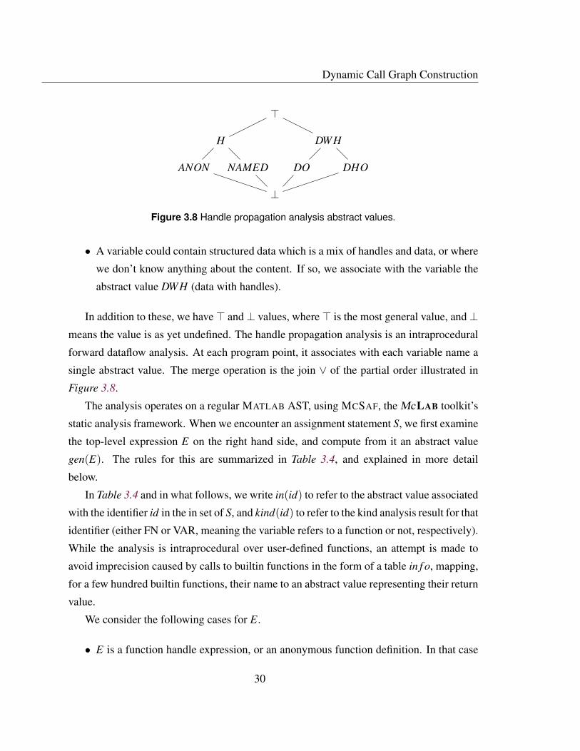
3.8 Handle propagation analysis abstract values. . . . . . . . . . . . . . . . . . 30
3.9 A code snippet where a variable is used and assigned to in the same statement. 34
4.1 An example of the lossy parsing and unparsing roundtrip. . . . . . . . . . . 41
4.2 The Transformer API, encoded as a Java interface . . . . . . . . . . . . . . 42
4.3 A trivial implementation of the Transformer API . . . . . . . . . . . . . . 43
4.4 An illustration of wacky commenting practices. . . . . . . . . . . . . . . . 48
4.5 Using runtime checks and AST traversal to examine the context. . . . . . . 50
4.6 An example illustrating the need for synthesized parentheses. . . . . . . . . 50
4.7 The original implementation of the Inline Variable refactoring using plain
AST operations, and the new implementation against the Transformer API. 51
xi
4.8 The implementation of the Extract Function refactoring using the trans-
former API . . . . . . . . . . . . . . . . . . . . . . . . . . . . . . . . . . 53
xii

List of Tables
3.1 Call graph instrumentation benchmarks. . . . . . . . . . . . . . . . . . . . 26
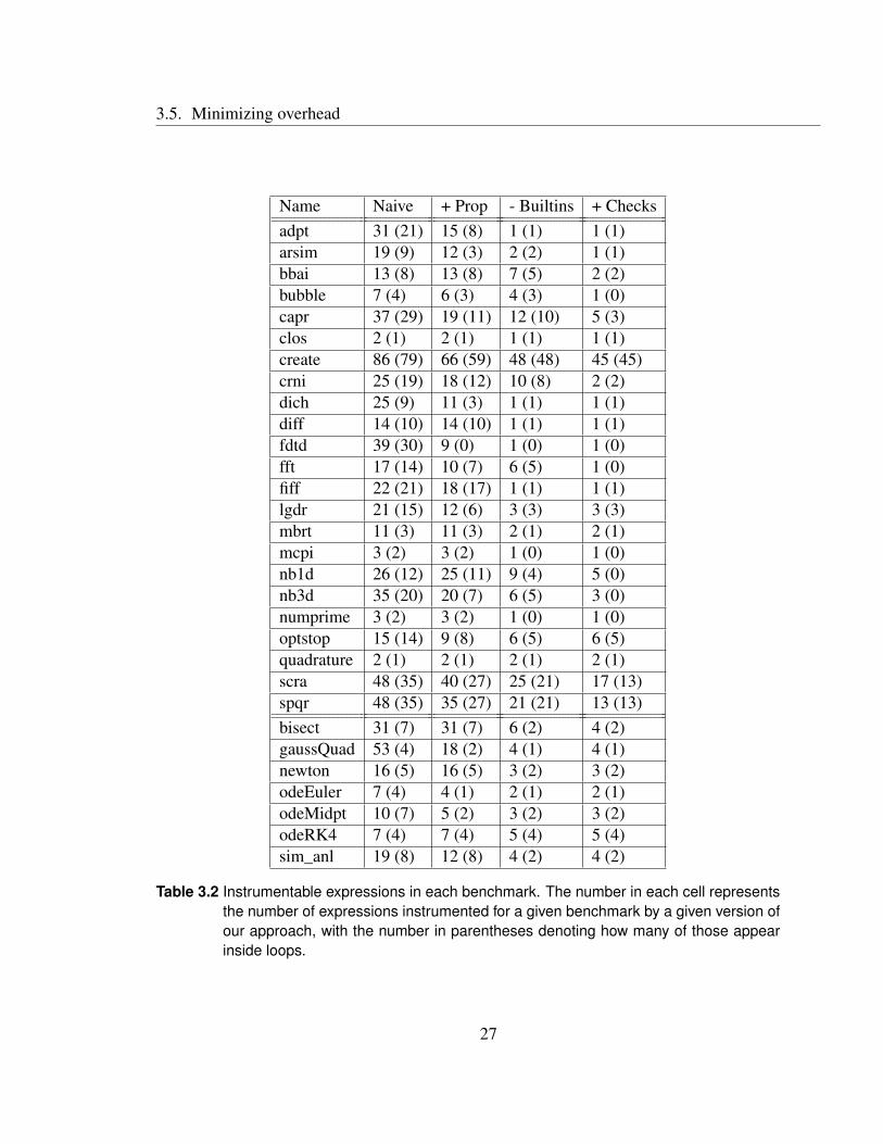
3.2 Instrumentable expressions in each benchmark. The number in each cell
represents the number of expressions instrumented for a given benchmark
by a given version of our approach, with the number in parentheses denot-
ing how many of those appear inside loops. . . . . . . . . . . . . . . . . . 27
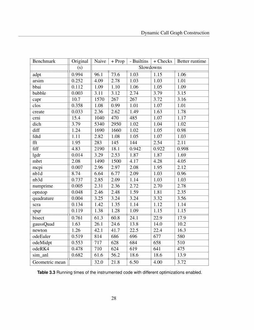
3.3 Running times of the instrumented code with different optimizations enabled. 28
3.4 Handle propagation analysis rules for computing gen(E). . . . . . . . . . . 31
3.5 Handle propagation analysis rules for assignments. . . . . . . . . . . . . . 34
5.1 File count per project distribution. . . . . . . . . . . . . . . . . . . . . . . 58
xiii

xiv
Chapter 1
Introduction
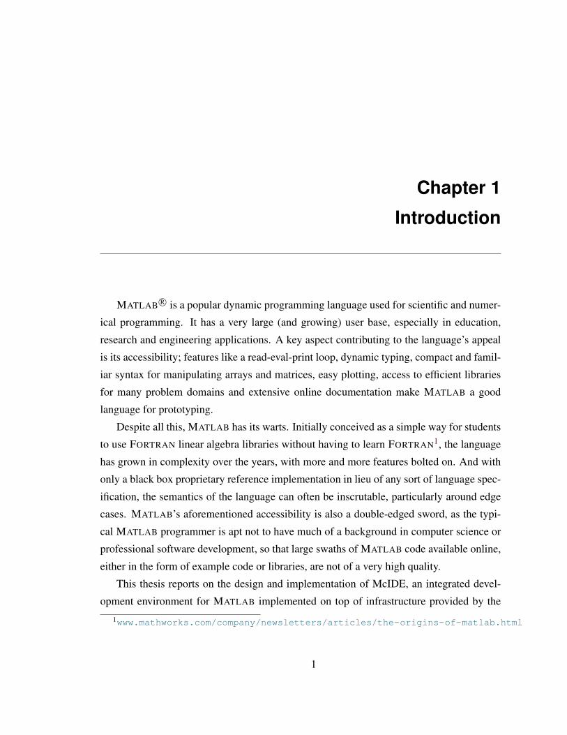
MATLAB R© is a popular dynamic programming language used for scientific and numer-
ical programming. It has a very large (and growing) user base, especially in education,
research and engineering applications. A key aspect contributing to the language’s appeal
is its accessibility; features like a read-eval-print loop, dynamic typing, compact and famil-
iar syntax for manipulating arrays and matrices, easy plotting, access to efficient libraries
for many problem domains and extensive online documentation make MATLAB a good
language for prototyping.
Despite all this, MATLAB has its warts. Initially conceived as a simple way for students
to use FORTRAN linear algebra libraries without having to learn FORTRAN1, the language
has grown in complexity over the years, with more and more features bolted on. And with
only a black box proprietary reference implementation in lieu of any sort of language spec-
ification, the semantics of the language can often be inscrutable, particularly around edge
cases. MATLAB’s aforementioned accessibility is also a double-edged sword, as the typi-
cal MATLAB programmer is apt not to have much of a background in computer science or
professional software development, so that large swaths of MATLAB code available online,
either in the form of example code or libraries, are not of a very high quality.
This thesis reports on the design and implementation of McIDE, an integrated devel-
opment environment for MATLAB implemented on top of infrastructure provided by the
1www.mathworks.com/company/newsletters/articles/the-origins-of-matlab.html
1

Introduction
McLAB compiler toolkit [CLD+10]. In addition to providing many traditional IDE fea-
tures such as easy code navigation and support for refactorings, McIDE also aims to im-
prove the state of MATLAB code in the wild, be it in terms of performance, complexity,
or amenableness to static analysis, by recognizing common anti-patterns in MATLAB code
and warning about them.
1.1 Contributions
The major contributions of this thesis are as follows.
A mechanism for computing a dynamic call graph of MATLAB code: Many traditional
code navigation features provided by IDEs, such as "jump to declaration" or "find
callers", rely on call graph information. However, MATLAB’s semantics make it dif-
ficult to statically compute a program’s call graph. We present a dynamic profiling
approach to measure a MATLAB program’s call graph, and describe some optimiza-
tions we implemented to reduce the overhead of the instrumentation required for the
profiling.
A technique for carrying out layout preserving code transformations: One of the most
useful features commonly provided by IDEs is automated refactoring support. The
most natural and straightforward way to implement a refactoring is as a tree transfor-
mation on a program’s abstract syntax tree. However, such transformations are lossy,
as the textual layout of the source code, including comments, indentation and other
whitespace, are lost in the process. We report on the design and implementation of
a library which enables arbitrary source code transformations to be specified at the
AST level, while the underlying machinery transparently takes care of preserving the
layout of the affected text.
A study of the usage of MATLAB’s dynamic features in the wild: MATLAB supports many
highly dynamic features, such as the eval family of functions, which complicate
static analysis, harm performance, and often make code harder to reason about. We
2
1.2. Thesis outline
describe the semantics of these features in detail, and report the results of a study of
a large corpus of MATLAB code, investigating the usage patterns of these features.
An open implementation: McIDE is developed fully in the open, on top of the open
source McLAB compiler toolkit for MATLAB. Some of the reusable infrastructure
pieces, such as the layout preserving transformation engine, are implemented di-
rectly as part of the toolkit, while the IDE itself is available as a separate open source
project2.
1.2 Thesis outline
The rest of the thesis is structured as follows. Chapter 2 provides some necessary back-
ground information and describes the overall structure of our IDE. The next three chapters
comprise largely independent in-depth explorations into its different components.
• Chapter 3 explains our approach to computing a dynamic call graph for MATLAB
programs, which is used to power the IDE’s code navigation features.
• Chapter 4 describes our layout preserving program transformation library, which is
used to implement the mechanics of the refactoring transformations supported by
McIDE.
• Chapter 5 presents our investigation into the usage of MATLAB’s dynamic features.
Finally, Chapter 6 concludes the thesis and describes some opportunities for future
work.
2www.sable.mcgill.ca/mclab/projects/mcide/
3

Introduction
4

Chapter 2
Background and Overview
2.1 McLab toolkit
The McLAB toolkit is a collection of useful tools and infrastructure for dealing with MAT-
LAB code. It includes a MATLAB parser, and an intraprocedural static analysis framework
with some useful foundational analyses provided out of the box, such as reaching defini-
tions and the kind analysis for MATLAB [DHR].
It actually includes much more, including call graph construction and sophisticated type
and shape inference. However, much of this prior work was motivated by the ultimate goal
of compiling MATLAB to a static language such as FORTRAN or X10. In this context, it
was considered acceptable to carve out a reasonable subset of MATLAB code and rule out
any code considered too dynamic or "wild" to map cleanly onto static semantics. Thus,
many of the more sophisticated analyses assume that many of the features of MATLAB that
are difficult to handle simply don’t occur.
Since we wish to support the development of arbitrary MATLAB code, many of these
assumptions don’t hold for us, leaving many components of the toolkit off-limits for us.
A related issue is that since we wish to manipulate and reason about MATLAB source
code, we find ourselves working directly with high-level ASTs, eschewing simplifications
or lower-level IRs.
5

Background and Overview
2.2 Overall design
McIDE wires together many independent components into a coherent whole. While it runs
locally on the user’s computer, its interface is browser-based, and largely centered around
an instance of the Ace editor1, a well-known open source embeddable text editor compo-
nent. This browser-based interface contains almost no important logic; instead, it reacts
to user actions by sending HTTP requests to a server process, which then dispatches the
work to the appropriate component. These components, such as the parser, static analyz-
ers, automated refactorers, and so on, are all implemented as separate standalone tools,
which simply accept input and produce output. The dispatcher orchestrates these compo-
nents, typically by spawning them as child processes and monitoring their standard output
and error streams (shelling out to them, in Unix parlance), although other means of inter-
process communication would also work. This can be seen as a kind of service-oriented
architecture.
There are several advantages to structuring McIDE in this way. For one thing, it re-
moves the need to grapple with a large monolithic codebase. The different components can
be developed and maintained in isolation, and also reused in different ways, for example
as command line utilities, or as text editor plugins. Arbitrary, pre-existing components can
also be integrated into McIDE, with only a little effort required to wrap them in a suitable
interface. For example, various bits of functionality, such as the parser, are provided by
pre-existing components of the McLAB toolkit, and exposed to McIDE via simple shell
script wrappers.
The browser-based interface is harder to justify. It is not really a given that implement-
ing the interface using HTML and JavaScript is preferable to writing a traditional native
desktop application using one of the popular cross-platform UI toolkits. The main reason
is that a natural next step is to generalize McIDE to be a proper web application – a "cloud"
IDE, accessible over the Internet – and that less engineering effort would be required to port
it to that setting. The client-server separation also enforces in some sense that the interface
logic be decoupled from the domain logic.
1http://ace.c9.io/
6

2.2. Overall design
The remainder of this section shows some specific examples of how different compo-
nents are integrated at a high-level.
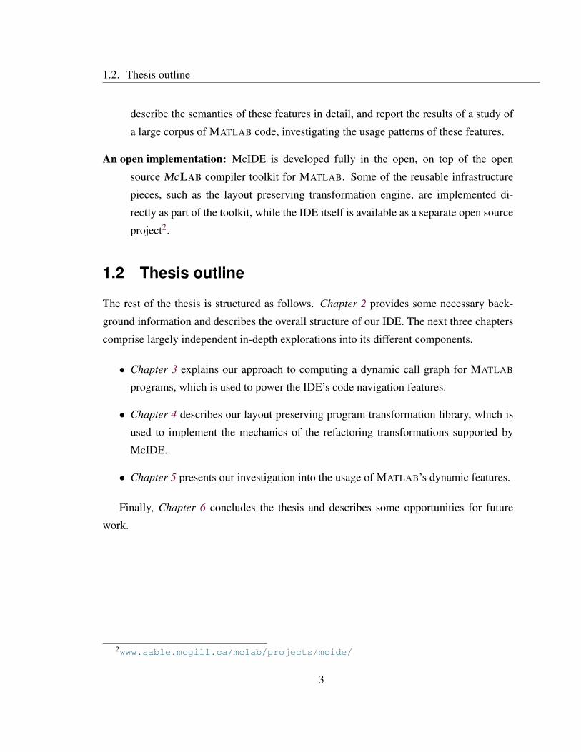
2.2.1 Syntax checking and static analysis
One of McIDE’s basic features is on-the-fly syntax checking. As the user types, the con-
tents of the editor are periodically sent off to the server as a "parse" request. Upon receiving
this request, the server spawns the McLAB toolkit’s MATLAB parser, ultimately returning
to the frontend either a serialized AST which can be used as input to other components,
or a list of syntax errors, each with associated line and column location information, to be
overlaid in the margins of the editor.
This workflow is sketched out in Figure 2.1. At the top, the user has just finished typing
in some code. The client sends an HTTP request to the server with the code as the request
body. The server calls the parser wrapper script, passing in the name of a temporary file
containing the code. The script prints some errors on standard output, and the server uses
these to build a JSON response that it returns to the client, which uses it to display an error
marker at the offending line, with the error messages displayed on mouse over.
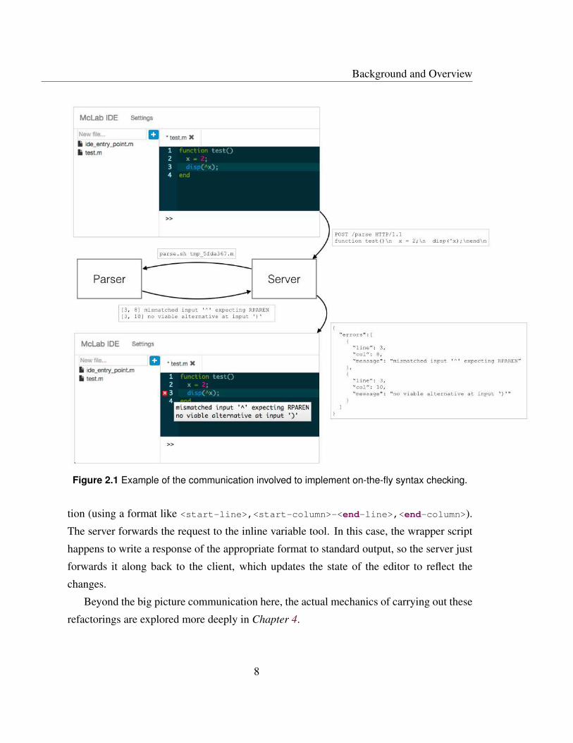
2.2.2 Refactoring
McIDE supports many automated refactorings, such as Extract Function or Inline Variable.
A refactoring can be viewed as a function taking as input some code and a user selection
(e.g. a highlighted region) and returning either the transformed code or an error. This fits
nicely into our model. When the user selects some code and selects a refactoring action
from a menu, the frontend sends the project path, the selection, and the choice of refactoring
off to the server as a "refactor" request. (It sends project paths rather than sending the code
directly in case the refactoring affects multiple files). This request is dispatched to the
appropriate refactoring tool, which responds either with a list of errors, or with a mapping
from affected file names to new contents.
This workflow is sketched out in Figure 2.2. The user has highlighted an assignment
statement and selected the "Inline Variable" action from the context menu. The client sends
an HTTP request to the server with the choice of refactoring, the active file, and the selec-
7
Background and Overview
Figure 2.1 Example of the communication involved to implement on-the-fly syntax checking.
tion (using a format like <start-line>,<start-column>-<end-line>,<end-column>).
The server forwards the request to the inline variable tool. In this case, the wrapper script
happens to write a response of the appropriate format to standard output, so the server just
forwards it along back to the client, which updates the state of the editor to reflect the
changes.
Beyond the big picture communication here, the actual mechanics of carrying out these
refactorings are explored more deeply in Chapter 4.
8
2.2. Overall design
Figure 2.2 Example of the communication involved to implement refactorings.
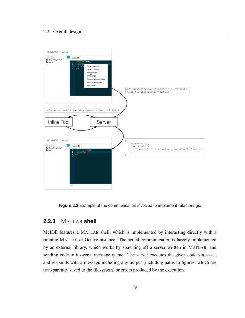
2.2.3 MATLAB shell
McIDE features a MATLAB shell, which is implemented by interacting directly with a
running MATLAB or Octave instance. The actual communication is largely implemented
by an external library, which works by spawning off a server written in MATLAB, and
sending code to it over a message queue. The server executes the given code via eval,
and responds with a message including any output (including paths to figures, which are
transparently saved to the filesystem) or errors produced by the execution.
9

Background and Overview
When the user starts working on a project, such a MATLAB server is initialized in the
background, and a command prompt is presented to the user alongside the editor. Any
commands entered are sent off to the dispatching server as a "shell command" request,
which forwards them along to the MATLAB server, and returns the results back to the
frontend, which can display output and error messages in its shell, and open new browser
windows or tabs to display figures.
McIDE also interacts with the MATLAB server behind the scenes for various reasons.
• When a function is called, MATLAB loads the function’s code from the filesystem and
caches the function. This cache is refreshed each time the command prompt is shown,
so that if a function is modified, MATLAB will notice that the last modified timestamp
has changed and reload the function. Due to the nature of our communication with
the MATLAB server, this refresh mechanism doesn’t happen. For situations like these,
MATLAB provides the rehash builtin function to force the caches to be refreshed.
McIDE therefore prepends a call to rehash to every command entered by the user
before sending it off.
• After each command entered by the user, McIDE appends a call to the save MAT-
LAB builtin function in order to store the state of the interpreter session to a hidden
file associated with the project. When the same project is loaded later, this session
file is loaded via the builtin load function, so that all the variables are preserved.
A nice bonus is that the format of the files produced by save and loaded by load
are compatible across MATLAB and Octave, so the backend can be changed in the
settings menu without losing any active sessions.
• The proprietary MATLAB implementation provides a workspace browser, a graphi-
cal window allowing the user to view (and modify) all the variables in the current
workspace. To replicate this functionality, McIDE makes use of the MATLAB builtin
function whos, which lists all the variables in scope.
The overall workflow is sketched out in Figure 2.3. The user types in a call to the func-
tion test, which is the one being edited, and presses the return key. The client sends an
HTTP request to the server with the code to run. The server wraps the user’s code with
10
2.2. Overall design
Figure 2.3 Example of the communication involved to implement the MATLAB shell.
some code of its own as described above, and sends the execution request to an instance of
the MATLAB server, which has been pre-initialized to execute in the project’s workspace.
The MATLAB server responds with information about whether the code triggered any er-
rors (here the request was successful), what the output was (here "2" surrounded by some
whitespace), and whether there were any figures (not in this case). The server sends this
response back to the client, which displays the result of the command in the shell.
11

Background and Overview
2.2.4 Profiling
A big theme of McIDE’s implementation is the reliance on runtime information, since pre-
cise static information is often difficult to come by if we wish to handle arbitrary MATLAB
code. When a project is created or imported, McIDE automatically creates a special file
called mcide_entry_point.m, in which the user is asked to implement a function that exer-
cises as much of the project’s code as possible. Periodically, and also in response to certain
user actions, a profiling run is triggered, in the form of a "profile" request sent off to the
server. In response, an instrumented version of the project is created via a source-to-source
transformation, and the entry point function is invoked (via the same mechanism used to
implement the MATLAB shell) to gather runtime information.
Currently, the main user of this mechanism is the the dynamic call graph generator
described in Chapter 3, where the profiling run records the targets of each call site, but
the same mechanism could be used to gather, for instance, runtime types, or performance
profiling information.
12
Chapter 3
Dynamic Call Graph Construction
Modern IDEs provide many useful code navigation facilities, for instance allowing
users to jump from a call site to the declaration of the called function, or to find all the
call sites of a particular function definition. The reliability of such features is contingent on
the availability of accurate call graph information. However, MATLAB’s dynamic typing
and dynamic features complicate the problem of statically computing a precise call graph.
Previous work on MATLAB call graph construction operated on a MATLAB subset,
carefully ruling out those features which aren’t amenable to static analysis, with the ulti-
mate goal of compiling MATLAB to a statically typed language such as FORTRAN or X10
[DH12]. As we mean to support regular MATLAB development, carving out such a subset
is not an acceptable approach.
In this chapter, we present our approach to computing an accurate call graph for ar-
bitrary MATLAB code. Rather than relying on static analysis, we extract this information
dynamically, by instrumenting the input programs and tracing their actual execution on a
MATLAB implementation. This allows us to provide precise code navigation even in the
presence of features that have traditionally been hard to reason about statically, such as
calls to eval. This precision comes at the cost of soundness, as the computed call graphs
are correct only with respect to a set of recorded program runs, and some extra work for
the programmer, whose responsibility it becomes to provide entry points into the project
that cover enough code to be useful.
13
Dynamic Call Graph Construction
3.1 MATLAB features complicating static call graph com-
putation
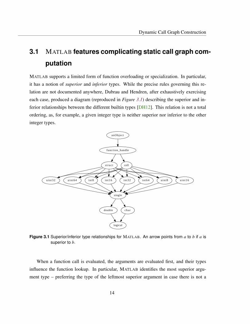
MATLAB supports a limited form of function overloading or specialization. In particular,
it has a notion of superior and inferior types. While the precise rules governing this re-
lation are not documented anywhere, Dubrau and Hendren, after exhaustively exercising
each case, produced a diagram (reproduced in Figure 3.1) describing the superior and in-
ferior relationships between the different builtin types [DH12]. This relation is not a total
ordering, as, for example, a given integer type is neither superior nor inferior to the other
integer types.
single
double cha r
logical
in t8 in t16 in t32 in t64 u in t8 u in t16u in t32 u in t64
function_handle
s t ruc t cell
anObject
Figure 3.1 Superior/inferior type relationships for MATLAB. An arrow points from a to b if a is
superior to b.
When a function call is evaluated, the arguments are evaluated first, and their types
influence the function lookup. In particular, MATLAB identifies the most superior argu-
ment type – preferring the type of the leftmost superior argument in case there is not a
14

3.2. Call graph tracing instrumentation
unique superior type – and uses this as the call site’s "dominant type", say char. Then, a
function defined in any directory named @char/ on MATLAB’s path will have priority over
other user-defined functions with the same name (with the exception of functions nested
inside the call site’s enclosing function). Thus, in order to statically compute a call graph
in the presence of specialized functions, we need to carry out type inference analysis to
approximate these lookup semantics.
Although MATLAB’s functions are not quite first-class, a special kind of object called a
function handle can be used as a reference to a function, either named or anonymous. These
handles can be stored in variables, as well as passed and returned from functions. Thus, in
order to statically compute a call graph in the presence of function handles, interprocedural
analysis is required to track which variables might hold function handles, and also which
functions each of these might point to.
In addition to these more traditional challenges, MATLAB supports many highly dy-
namic features that complicate any form of static analysis. Among these are the evaluation
of arbitrary strings as code via calls to the eval family of functions, and a function lookup
mechanism that involves crawling the filesystem at runtime – starting from a current direc-
tory that can be changed at runtime – in search of applicable call targets. More attention is
paid to these in Chapter 5.
3.2 Call graph tracing instrumentation
Since static analysis of MATLAB code is difficult and easily misled in the presence of
dynamic features, we rely on dynamic analysis to extract information that is sufficiently
precise for our needs. Denker et al. [DGL06] identify different approaches available to
dynamic analysis tool developers for gathering runtime data:
• Source code modification and, relatedly, logging services. This is the approach we
ultimately use, as we discuss later.
• Bytecode modification or instrumenting the virtual machine. This requires knowl-
edge of the internals of the MATLAB virtual machine, and as the reference MATLAB
implementation is a proprietary closed-source black box, this isn’t an option for us.
15

Dynamic Call Graph Construction
• Method wrappers. This refers to some mechanism for introducing code to be exe-
cuted before, after, or instead of a function. Our particular source-to-source transfor-
mation, described later, can be seen of an instance of this technique.
• Debuggers. While the reference MATLAB implementation does include a debugger,
we prefer not to couple ourselves too tightly to it, as it is not under our control.
The most natural and portable approach is source code modification. We can implement
it using the infrastructure provided as part of the McLAB toolkit.
The high-level idea is to insert logging statements before every possible call site, and
at the start of every function or script. After executing the transformed code, we can post-
process the logs and match up call sites with their targets, since the target will follow the
call in the log. We define a unique identifier identi f ier(n) for every call site and call target
n; this consists of the name of n (the variable name if it’s a variable, the function name if
it’s a function definition, the script name if it’s a script, and the string <lambda> if it’s an
anonymous function expression), the file it’s contained in and its position (line and column)
within that file. This format comes in handy when it comes to implementing navigation
features in an IDE, as these typically take a textual range (e.g. a mouse selection) as input.
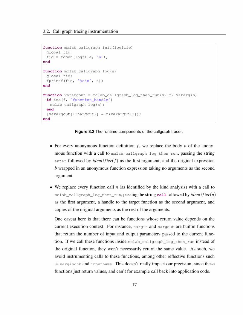
The transformation depends on a few functions (listed in Figure 3.2) being available at
runtime. The mclab_callgraph_init and mclab_callgraph_log functions are straight-
forward; the former takes a path to a log file, creates it and makes a handle to it globally
accessible, while the latter takes a string and writes it to the file.
mclab_callgraph_log_then_run is more complicated; it takes a string, a variable (which
is possibly a function handle) and a variable number of arguments. If the given variable is a
function handle (either a function handle expression, or a variable that contains a function
handle), then we log the string to the file, and in either case we forward the arguments to
the variable.
Assuming these runtime functions are available, we traverse the whole project and per-
form the following transformations.
• For every function or script f , we insert a call to mclab_callgraph_log as the first
statement, passing the string enter followed by identi f ier( f ).
16
3.2. Call graph tracing instrumentation
function mclab_callgraph_init(logfile)
global fid
fid = fopen(logfile, ’a’);
end
function mclab_callgraph_log(s)
global fid;
fprintf(fid, ’%s\n’, s);
end
function varargout = mclab_callgraph_log_then_run(s, f, varargin)
if isa(f, ’function_handle’)
mclab_callgraph_log(s);
end
[varargout{1:nargout}] = f(varargin{:});
end
Figure 3.2 The runtime components of the callgraph tracer.
• For every anonymous function definition f , we replace the body b of the anony-
mous function with a call to mclab_callgraph_log_then_run, passing the string
enter followed by identi f ier( f ) as the first argument, and the original expression
b wrapped in an anonymous function expression taking no arguments as the second
argument.
• We replace every function call n (as identified by the kind analysis) with a call to
mclab_callgraph_log_then_run, passing the string call followed by identi f ier(n)
as the first argument, a handle to the target function as the second argument, and
copies of the original arguments as the rest of the arguments.
One caveat here is that there can be functions whose return value depends on the
current execution context. For instance, nargin and nargout are builtin functions
that return the number of input and output parameters passed to the current func-
tion. If we call these functions inside mclab_callgraph_log_then_run instead of
the original function, they won’t necessarily return the same value. As such, we
avoid instrumenting calls to these functions, among other reflective functions such
as narginchk and inputname. This doesn’t really impact our precision, since these
functions just return values, and can’t for example call back into application code.
17

Dynamic Call Graph Construction
• While the kind analysis distinguishes between function calls and variable accesses, it
doesn’t distinguish among the latter between array accesses and function handle in-
vocations. In order to accurately trace control flow through function handles, we also
instrument variable accesses in the same way as for function calls, only rather than
passing in a function handle expression as the second argument, we just pass in the
variable. At runtime, mclab_callgraph_log_then_run makes use of MATLAB’s
reflective features to identify function handles, and only logs the call event in those
cases. One small detail here is that an array access might have a colon literal as one
of its arguments, and passing it to a function instead will cause MATLAB to generate
an error at runtime. In order for the transformation to be correct, we go through and
replace any colon literals with colon string literals.
Finally, in order to trigger a tracing execution, an entry point is needed – that is, a
piece of code that will attempt to exercise as much of the subject code as possible. This
is handed off to the tracing machinery, which will first instrument the project as described
(in a temporary folder), create a temporary file to hold the trace, and invoke MATLAB, first
calling mclab_callgraph_init with the path to the log file, and then the entry point. Once
the execution is over, the trace is processed, and call graph edges are identified by looking
for call events that are immediately followed by an enter event.
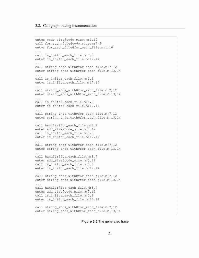
Figure 3.3, Figure 3.4, Figure 3.5 and Figure 3.6 together show an end-to-end example.
• Figure 3.3 shows the application code. for_each_file recursively traverses a di-
rectory tree (using the builtin function dir as a primitive) and invokes a passed-in
handler for each file with the given extension, making use of the helper functions
string_ends_with and is_in along the way. code_size calls for_each_file,
passing in a handle to the nested function add_size as the handler. In MATLAB,
nested functions are closures, so that add_size can read and write to the total_size
variable in the enclosing scope. In this way, code_size adds up the sizes of all the
m-files in the current directory.
• Figure 3.4 shows the same code after instrumentation (with all instances of the
mclab_callgraph_ prefix omitted for brevity).
18

3.2. Call graph tracing instrumentation
• Figure 3.5 shows the generated trace, using an invocation of code_size() as the
entry point. Some events are omitted for brevity.
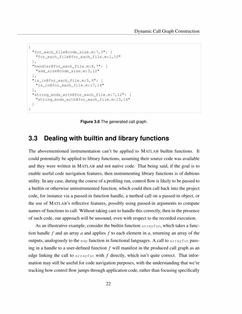
• Finally, Figure 3.6 shows the call graph produced by processing the trace and match-
ing up call and enter events. The call graph is in JSON format, mapping, for each
covered call site, the call site’s identifier to an array of function identifiers.
function for_each_file(root, extension, handler)
files = dir(root);
for i = 1:numel(files)
file = files(i);
if ~is_in({’.’, ’..’}, file.name) && file.isdir
for_each_file(fullfile(root, file.name), extension, handler)
elseif string_ends_with(extension, file.name)
handler(file)
end
end
end
function b = string_ends_with(suffix, s)
b = strfind(s, suffix) == length(s) - length(suffix) + 1;
end
function b = is_in(strings, string)
b = ~isempty(find(ismember(strings, string)));
end
function code_size
total_size = 0;
function add_size(file)
total_size = total_size + file.bytes;
end
for_each_file(’.’, ’.m’, @add_size);
disp(total_size);
end
Figure 3.3 The application code.
19

Dynamic Call Graph Construction
function [] = for_each_file(root, extension, handler)
_log(’enter for_each_file@for_each_file.m:1,10’);
files = _log_then_run(’call dir@for_each_file.m:2,11’, @dir, root);
for i = (1 : _log_then_run(’call numel@for_each_file.m:3,13’, @numel,
files))
file = _log_then_run(’call files@for_each_file.m:4,12’, files, i);
if ((~_log_then_run(’call is_in@for_each_file.m:5,9’, @is_in, {’.’,
’..’}, file.name)) && file.isdir)
_log_then_run(’call for_each_file@for_each_file.m:6,7’,
@for_each_file, _log_then_run(’call
fullfile@for_each_file.m:6,21’, @fullfile, root, file.name),
extension, handler)
elseif _log_then_run(’call string_ends_with@for_each_file.m:7,12’,
@string_ends_with, extension, file.name)
_log_then_run(’call handler@for_each_file.m:8,7’, handler, file)
end
end
end
function [b] = string_ends_with(suffix, s)
_log(’enter string_ends_with@for_each_file.m:13,14’);
b = (_log_then_run(’call strfind@for_each_file.m:14,7’, @strfind, s,
suffix) == ((_log_then_run(’call length@for_each_file.m:14,29’,
@length, s) - _log_then_run(’call length@for_each_file.m:14,41’,
@length, suffix)) + 1));
end
function [b] = is_in(strings, string)
_log(’enter is_in@for_each_file.m:17,14’);
b = (~_log_then_run(’call isempty@for_each_file.m:18,8’, @isempty,
_log_then_run(’call find@for_each_file.m:18,16’, @find,
_log_then_run(’call ismember@for_each_file.m:18,21’, @ismember,
strings, string))));
end
function [] = code_size()
_log(’enter code_size@code_size.m:1,10’);
total_size = 0;
_log_then_run(’call for_each_file@code_size.m:7,3’, @for_each_file,
’.’, ’.m’, @add_size);
_log_then_run(’call disp@code_size.m:8,3’, @disp, total_size);
function [] = add_size(file)
_log(’enter add_size@code_size.m:3,12’);
total_size = (total_size + file.bytes);
end
end
Figure 3.4 The same code after instrumentation.
20
3.2. Call graph tracing instrumentation
enter code_size@code_size.m:1,10
call for_each_file@code_size.m:7,3
enter for_each_file@for_each_file.m:1,10
...
call is_in@for_each_file.m:5,9
enter is_in@for_each_file.m:17,14
...
call string_ends_with@for_each_file.m:7,12
enter string_ends_with@for_each_file.m:13,14
...
call is_in@for_each_file.m:5,9
enter is_in@for_each_file.m:17,14
...
call string_ends_with@for_each_file.m:7,12
enter string_ends_with@for_each_file.m:13,14
...
call is_in@for_each_file.m:5,9
enter is_in@for_each_file.m:17,14
...
call string_ends_with@for_each_file.m:7,12
enter string_ends_with@for_each_file.m:13,14
...
call handler@for_each_file.m:8,7
enter add_size@code_size.m:3,12
call is_in@for_each_file.m:5,9
enter is_in@for_each_file.m:17,14
...
call string_ends_with@for_each_file.m:7,12
enter string_ends_with@for_each_file.m:13,14
...
call handler@for_each_file.m:8,7
enter add_size@code_size.m:3,12
call is_in@for_each_file.m:5,9
enter is_in@for_each_file.m:17,14
...
call string_ends_with@for_each_file.m:7,12
enter string_ends_with@for_each_file.m:13,14
...
call handler@for_each_file.m:8,7
enter add_size@code_size.m:3,12
call is_in@for_each_file.m:5,9
enter is_in@for_each_file.m:17,14
...
call string_ends_with@for_each_file.m:7,12
enter string_ends_with@for_each_file.m:13,14
Figure 3.5 The generated trace.
21
Dynamic Call Graph Construction
{
"for_each_file@code_size.m:7,3": [
"for_each_file@for_each_file.m:1,10"
],
"handler@for_each_file.m:8,7": [
"add_size@code_size.m:3,12"
],
"is_in@for_each_file.m:5,9": [
"is_in@for_each_file.m:17,14"
],
"string_ends_with@for_each_file.m:7,12": [
"string_ends_with@for_each_file.m:13,14"
]
}
Figure 3.6 The generated call graph.
3.3 Dealing with builtin and library functions
The abovementioned instrumentation can’t be applied to MATLAB builtin functions. It
could potentially be applied to library functions, assuming their source code was available
and they were written in MATLAB and not native code. That being said, if the goal is to
enable useful code navigation features, then instrumenting library functions is of dubious
utility. In any case, during the course of a profiling run, control flow is likely to be passed to
a builtin or otherwise uninstrumented function, which could then call back into the project
code, for instance via a passed-in function handle, a method call on a passed-in object, or
the use of MATLAB’s reflective features, possibly using passed-in arguments to compute
names of functions to call. Without taking care to handle this correctly, then in the presence
of such code, our approach will be unsound, even with respect to the recorded execution.
As an illustrative example, consider the builtin function arrayfun, which takes a func-
tion handle f and an array a and applies f to each element in a, returning an array of the
outputs, analogously to the map function in functional languages. A call to arrayfun pass-
ing in a handle to a user-defined function f will manifest in the produced call graph as an
edge linking the call to arrayfun with f directly, which isn’t quite correct. That infor-
mation may still be useful for code navigation purposes, with the understanding that we’re
tracking how control flow jumps through application code, rather than focusing specifically
22
3.3. Dealing with builtin and library functions
on call sites and their targets, but there again that’s beyond the scope of a call graph com-
putation. A bigger problem occurs if f itself calls a builtin function c, as control would
flow back to arrayfun which would invoke f again, linking together the call to c with f .
Unlike the previous case, this has no practical application, and is just wrong.
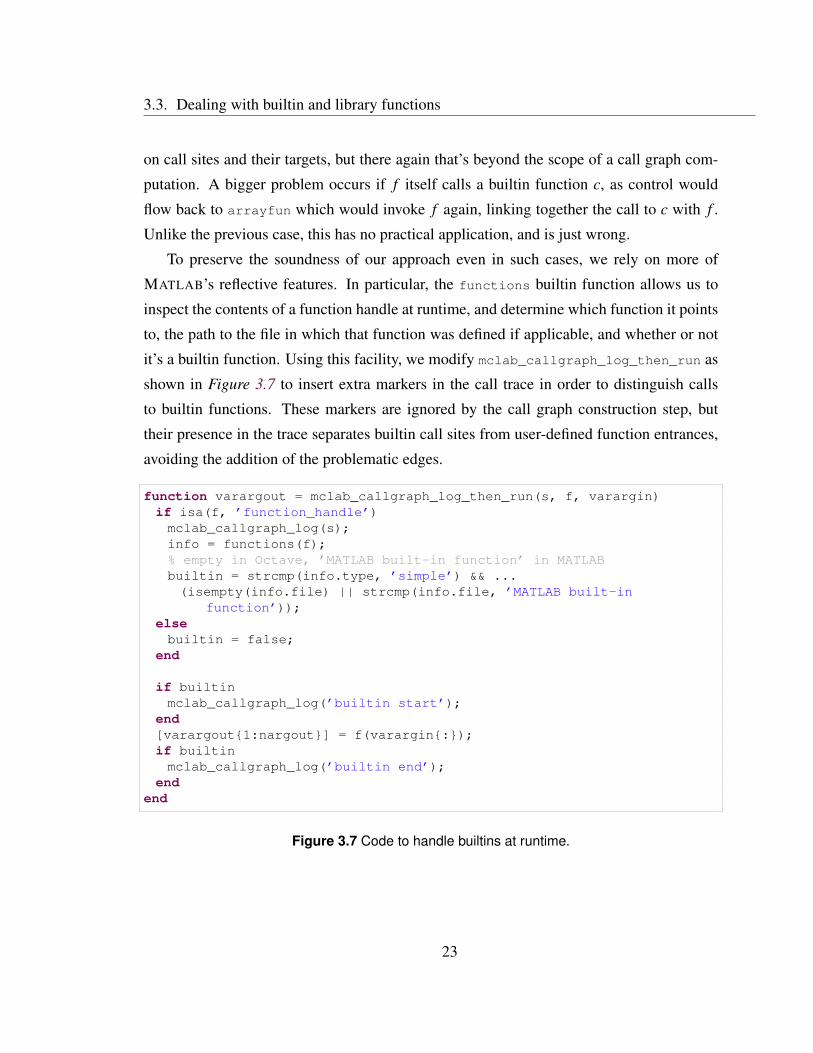
To preserve the soundness of our approach even in such cases, we rely on more of
MATLAB’s reflective features. In particular, the functions builtin function allows us to
inspect the contents of a function handle at runtime, and determine which function it points
to, the path to the file in which that function was defined if applicable, and whether or not
it’s a builtin function. Using this facility, we modify mclab_callgraph_log_then_run as
shown in Figure 3.7 to insert extra markers in the call trace in order to distinguish calls
to builtin functions. These markers are ignored by the call graph construction step, but
their presence in the trace separates builtin call sites from user-defined function entrances,
avoiding the addition of the problematic edges.
function varargout = mclab_callgraph_log_then_run(s, f, varargin)
if isa(f, ’function_handle’)
mclab_callgraph_log(s);
info = functions(f);
% empty in Octave, ’MATLAB built-in function’ in MATLAB
builtin = strcmp(info.type, ’simple’) && ...
(isempty(info.file) || strcmp(info.file, ’MATLAB built-in
function’));
else
builtin = false;
end
if builtin
mclab_callgraph_log(’builtin start’);
end
[varargout{1:nargout}] = f(varargin{:});
if builtin
mclab_callgraph_log(’builtin end’);
end
end
Figure 3.7 Code to handle builtins at runtime.
23
Dynamic Call Graph Construction
3.4 Instrumentation performance overhead
A priori, we expect the instrumented code to run at least an order of magnitude or two
slower than the original code, the main culprit being the wrapping of every single function
call or variable access with a call to an auxiliary function. In order to get a sense of the
magnitude of the overhead, we run some benchmarks with and without instrumentation.
3.4.1 Benchmarks
We run our experiments on a set of 29 MATLAB benchmarks. 23 of these are part of the
McLAB project’s standard benchmark suite, which was collected from various sources, in-
cluding the FALCON and OTTER projects, Chalmers University of Technology, the MAT-
LAB Central File Exchange, and the ACM CALGO library. These benchmarks are mostly
numerical algorithms, heavy on loops and array reads and writes, and not so heavy on
function calls or function handles. Most MATLAB code looks like this, so measuring and
minimizing overhead on such code is important. However, it’s also important to evaluate
our approach on code where the tracing would reveal useful information. To that end, we
also include seven additional benchmarks in our suite. Six of these are numerical solvers, a
class of programs where it is common to operate on function handles. These are the same
benchmarks used by Lameed and Hendren to evaluate their work on optimizing feval
implementations [LH13].
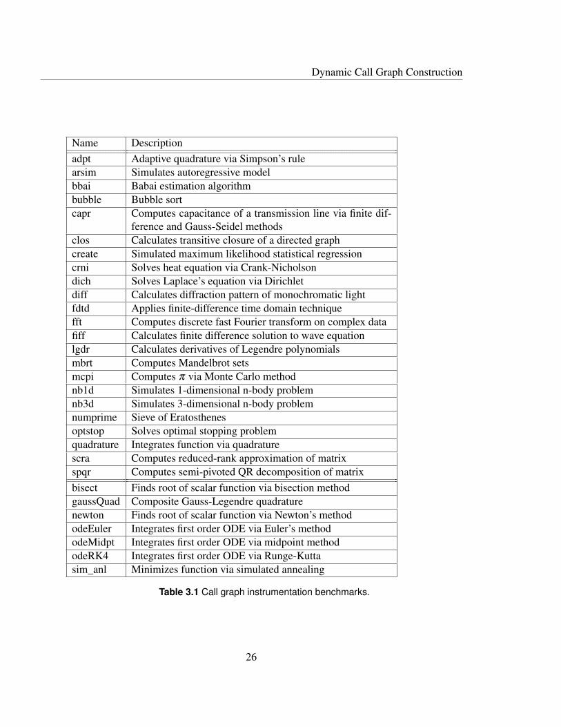
These benchmarks are described briefly in Table 3.1. In Table 3.2, we include some
simple static metrics to help understand the following experimental results. Since instru-
menting a function call or array access adds an overhead proportional to the number of
times it is executed, we note, for each benchmark, how many calls or accesses are in-
strumented (this is the first number in each column), and how many of these are inside
loops (this is the number in parentheses in each column). Note that this is computed is
a relatively simple-minded way, and doesn’t catch, for example, calls or accesses inside
functions which are called inside loops. Nevertheless, this can be an interesting metric.
The "Naive" column refers to the instrumentation described thus far. We then show how
each optimization described later in this section affects this metric (in other words, how
24

3.5. Minimizing overhead
many expressions we are able to avoid instrumenting). These are the "+ Prop", "- Builtins",
and "+ Checks" columns; their specific meanings are described in the following section.
3.4.2 Results
The results are shown in Table 3.3. All the programs were executed on a machine with
an Intel R© CoreTM i7 CPU @ 2.4 GHz and 8 GB of memory, running OS X 10.10, using
MATLAB version R2014b. For each benchmark, we show the running times of the original
code in seconds, and the slowdown of each instrumented version relative to the original
code. The columns refer to the same versions as in Table 3.2, and the specific meaning of
the "Better runtime" is given in the following section.
For the naive instrumentation described thus far, we see that the slowdown can be ex-
treme for some benchmarks, with six of the benchmarks (capr, carni, dich, diff, fiff and
mbrt) undergoing a three order of magnitude slowdown. All of these are in the numerical
category, and can be optimized. The functional benchmarks all see a slowdown between
one and two orders of magnitude. While we’re able to optimize them slightly, they tend to
stay within the same order of magnitude.
3.5 Minimizing overhead
The bulk of the runtime overhead of our approach stems from instrumenting each function
call and variable access, which is ultimately caused by our inability to precisely distinguish
arrays from function handles statically. Yet arrays are apt to be much more common than
function handles, so that the cost of instrumenting each array access is disproportionate
relative to the benefit. Thus, we apply a few different techniques to try and minimize the
amount of array accesses that require instrumentation.
3.5.1 Handle propagation analysis
While the McLAB toolkit doesn’t provide any facilities for performing interprocedural
static analysis on arbitrary MATLAB code, we can still track the flow of function handles
through a single function. For each use of a variable, we can estimate whether the variable
25
Dynamic Call Graph Construction
Name Description
adpt Adaptive quadrature via Simpson’s rulearsim Simulates autoregressive modelbbai Babai estimation algorithmbubble Bubble sortcapr Computes capacitance of a transmission line via finite dif-
ference and Gauss-Seidel methodsclos Calculates transitive closure of a directed graphcreate Simulated maximum likelihood statistical regressioncrni Solves heat equation via Crank-Nicholsondich Solves Laplace’s equation via Dirichletdiff Calculates diffraction pattern of monochromatic lightfdtd Applies finite-difference time domain techniquefft Computes discrete fast Fourier transform on complex datafiff Calculates finite difference solution to wave equationlgdr Calculates derivatives of Legendre polynomialsmbrt Computes Mandelbrot setsmcpi Computes π via Monte Carlo methodnb1d Simulates 1-dimensional n-body problemnb3d Simulates 3-dimensional n-body problemnumprime Sieve of Eratosthenesoptstop Solves optimal stopping problemquadrature Integrates function via quadraturescra Computes reduced-rank approximation of matrixspqr Computes semi-pivoted QR decomposition of matrix
bisect Finds root of scalar function via bisection methodgaussQuad Composite Gauss-Legendre quadraturenewton Finds root of scalar function via Newton’s methododeEuler Integrates first order ODE via Euler’s methododeMidpt Integrates first order ODE via midpoint methododeRK4 Integrates first order ODE via Runge-Kuttasim_anl Minimizes function via simulated annealing
Table 3.1 Call graph instrumentation benchmarks.
26
3.5. Minimizing overhead
Name Naive + Prop - Builtins + Checks
adpt 31 (21) 15 (8) 1 (1) 1 (1)arsim 19 (9) 12 (3) 2 (2) 1 (1)bbai 13 (8) 13 (8) 7 (5) 2 (2)bubble 7 (4) 6 (3) 4 (3) 1 (0)capr 37 (29) 19 (11) 12 (10) 5 (3)clos 2 (1) 2 (1) 1 (1) 1 (1)create 86 (79) 66 (59) 48 (48) 45 (45)crni 25 (19) 18 (12) 10 (8) 2 (2)dich 25 (9) 11 (3) 1 (1) 1 (1)diff 14 (10) 14 (10) 1 (1) 1 (1)fdtd 39 (30) 9 (0) 1 (0) 1 (0)fft 17 (14) 10 (7) 6 (5) 1 (0)fiff 22 (21) 18 (17) 1 (1) 1 (1)lgdr 21 (15) 12 (6) 3 (3) 3 (3)mbrt 11 (3) 11 (3) 2 (1) 2 (1)mcpi 3 (2) 3 (2) 1 (0) 1 (0)nb1d 26 (12) 25 (11) 9 (4) 5 (0)nb3d 35 (20) 20 (7) 6 (5) 3 (0)numprime 3 (2) 3 (2) 1 (0) 1 (0)optstop 15 (14) 9 (8) 6 (5) 6 (5)quadrature 2 (1) 2 (1) 2 (1) 2 (1)scra 48 (35) 40 (27) 25 (21) 17 (13)spqr 48 (35) 35 (27) 21 (21) 13 (13)
bisect 31 (7) 31 (7) 6 (2) 4 (2)gaussQuad 53 (4) 18 (2) 4 (1) 4 (1)newton 16 (5) 16 (5) 3 (2) 3 (2)odeEuler 7 (4) 4 (1) 2 (1) 2 (1)odeMidpt 10 (7) 5 (2) 3 (2) 3 (2)odeRK4 7 (4) 7 (4) 5 (4) 5 (4)sim_anl 19 (8) 12 (8) 4 (2) 4 (2)
Table 3.2 Instrumentable expressions in each benchmark. The number in each cell represents
the number of expressions instrumented for a given benchmark by a given version of
our approach, with the number in parentheses denoting how many of those appear
inside loops.
27
Dynamic Call Graph Construction
Benchmark Original Naive + Prop - Builtins + Checks Better runtime(s) Slowdowns
adpt 0.994 96.1 73.6 1.03 1.15 1.06arsim 0.252 4.09 2.78 1.03 1.03 1.01bbai 0.112 1.09 1.10 1.06 1.05 1.09bubble 0.003 3.11 3.12 2.74 3.79 3.15capr 10.7 1570 267 267 3.72 3.16clos 0.358 1.08 0.99 1.01 1.07 1.01create 0.033 2.36 2.62 1.49 1.63 1.78crni 15.4 1040 470 485 1.07 1.17dich 3.79 5340 2950 1.02 1.04 1.02diff 1.24 1690 1660 1.02 1.05 0.98fdtd 1.11 2.82 1.08 1.05 1.07 1.03fft 1.95 283 145 144 2.54 2.11fiff 4.83 2190 18.1 0.942 0.922 0.998lgdr 0.014 3.29 2.53 1.87 1.87 1.69mbrt 2.08 1490 1500 4.17 4.28 4.05mcpi 0.007 2.96 2.97 2.08 1.95 2.12nb1d 8.74 6.64 6.77 2.09 1.03 0.96nb3d 0.737 2.85 2.09 1.14 1.03 1.03numprime 0.005 2.31 2.36 2.72 2.70 2.78optstop 0.048 2.46 2.48 1.59 1.81 2.35quadrature 0.004 3.25 3.24 3.24 3.32 3.56scra 0.134 1.42 1.35 1.14 1.12 1.14spqr 0.119 1.38 1.28 1.09 1.15 1.15
bisect 0.761 61.3 60.8 24.1 22.9 17.9gaussQuad 1.63 26.1 24.6 13.8 14.0 10.2newton 1.26 42.1 41.7 22.5 22.4 16.3odeEuler 0.519 814 686 696 677 580odeMidpt 0.553 717 628 684 658 510odeRK4 0.478 710 624 619 641 475sim_anl 0.682 61.6 56.2 18.6 18.6 13.9
Geometric mean 32.0 21.8 6.50 4.00 3.72
Table 3.3 Running times of the instrumented code with different optimizations enabled.
28
3.5. Minimizing overhead
holds only data, or a function handle, or possibly a complex data structure with a mix of
data and handles. Where we’re able to determine that a variable is definitely an array con-
taining only data, we can avoid instrumenting it. Some prior work had been done in this
direction inside the McLAB framework in the form of an intraprocedural handle propaga-
tion analysis – work which we formalized and whose implementation we completed.
The handle propagation analysis aims to compute, at each program point, which vari-
ables possibly contain function handles. It’s common to characterize MATLAB as a lan-
guage where everything is a matrix – even a scalar value is actually a 1x1 matrix. Function
handles, however, are not matrices. Broadly, we distinguish between handles and struc-
tured data such as arrays, structs or cell arrays. Then among these two categories we make
some further distinctions. In particular, the analysis deals with abstract values defined as
follows.
• A variable could contain a function handle created via a function handle expression
@f, which simply creates a handle to named function f. If so, we associate with the
variable the abstract value NAMED( f ), keeping track of the name it points to.
• A variable could contain a function handle created via an anonymous function @(x)expr(x).
If so, we associate with the variable the abstract value ANON(n), where n is a refer-
ence to the anonymous function node in the AST.
• A variable could contain a function handle we don’t have further information about.
Typically this would happen if it was assigned the result of a call to a builtin function
known to return handles. In that case we associate with the variable the abstract value
HANDLE, abbreviated as H.
• A variable could contain structured data (for example a cell array), every element of
which is a function handle. If so, we associate with it the abstract value DHO (data,
handle only).
• A variable could contain structured data where the elements are known to definitely
not be handles. If so, we associate with it the abstract value DO (data only).
29
Dynamic Call Graph Construction
⊥
ANON NAMED
H
DO DHO
DWH
⊤
Figure 3.8 Handle propagation analysis abstract values.
• A variable could contain structured data which is a mix of handles and data, or where
we don’t know anything about the content. If so, we associate with the variable the
abstract value DWH (data with handles).
In addition to these, we have ⊤ and ⊥ values, where ⊤ is the most general value, and ⊥
means the value is as yet undefined. The handle propagation analysis is an intraprocedural
forward dataflow analysis. At each program point, it associates with each variable name a
single abstract value. The merge operation is the join ∨ of the partial order illustrated in
Figure 3.8.
The analysis operates on a regular MATLAB AST, using MCSAF, the McLAB toolkit’s
static analysis framework. When we encounter an assignment statement S, we first examine
the top-level expression E on the right hand side, and compute from it an abstract value
gen(E). The rules for this are summarized in Table 3.4, and explained in more detail
below.
In Table 3.4 and in what follows, we write in(id) to refer to the abstract value associated
with the identifier id in the in set of S, and kind(id) to refer to the kind analysis result for that
identifier (either FN or VAR, meaning the variable refers to a function or not, respectively).
While the analysis is intraprocedural over user-defined functions, an attempt is made to
avoid imprecision caused by calls to builtin functions in the form of a table in f o, mapping,
for a few hundred builtin functions, their name to an abstract value representing their return
value.
We consider the following cases for E.
• E is a function handle expression, or an anonymous function definition. In that case
30

3.5. Minimizing overhead
Expression E Abstract value gen(E)@name NAMED(name) (1)@(..)... ANON(@(..)...) (2)id in(id) if kind(id) =VAR (3)
in f o(id) if kind(id) = FN ∧ id ∈ in f o (4)⊤ if kind(id) = FN ∧ id 6∈ in f o (5)
id(. . .) in f o(id) if kind(id) = FN ∧ id ∈ in f o (6)⊤ if kind(id) = FN ∧ id 6∈ in f o (7)in f o( f ) if in(id) = NAMED( f )∧ f ∈ in f o (8)⊤ if in(id) ∈ {H,ANON,NAMED} (9)in(id) otherwise (10)
id{. . .} DO if in(id) = DO (11)id. · · · H if in(id) = DHO (12)id.(. . .) ⊤ if in(id) = DWH (13){E1, . . . ,En} struct(
{
gen(E1), . . . ,gen(En)}
) (14)[E1, . . . ,En]any other expression DO (15)
Table 3.4 Handle propagation analysis rules for computing gen(E).
we simply generate the appropriate NAMED or ANON abstract value. This corre-
sponds to rules (1) and (2).
• E is a use of an identifier id. In MATLAB, the parentheses can be omitted from a
function call – but not a function handle invocation – if no arguments are passed.
Thus E is either a variable access, or a call to named function. The kind analysis is
enough to distinguish between the two cases. If it’s a variable, we simply propagate
forward whatever information we had (rule (3)). If it’s a call to a function with has
an entry in in f o, we use it (rule (4)). Otherwise, it’s a call to an unknown function
which might return anything, so we use ⊤ (rule (5)).
• E is a parameterized expression id(. . .). As in the previous case, E could be a call to
named function which we either have information about or not – rules (6) and (7) in
Table 3.4 are identical to rules (4) and (5).
Because of the parentheses, this might be a function handle invocation. If in(id) =
NAMED( f ) – that is, a handle to a named function f – and we have an entry for f
31
Dynamic Call Graph Construction
in in f o, then we can use it (rule (8)). If we don’t know anything about f , or if id
contains a handle we don’t know anything about, then we treat this as an arbitrary
function call and use ⊤ (rule (9)).
Otherwise, id refers to a variable containing data – either an array or a cell array (but
not a struct, because structs can’t be accessed with parentheses). Arrays in MATLAB
can’t contain function handles. Cell arrays can contain handles, but indexing a cell
array with parentheses (rather than braces) doesn’t return the contained data directly,
instead returning a set of cells. Thus in this case we can again simply propagate
forward the information we already had for id (rule (10)).
• E could be a cell array indexing expression id{. . .}, or struct access expression id. · · ·
or id.(. . .). We treat all of these cases the same way. If id is known to only contain
data (DO), then all of its elements only contain data, so we can use DO again (rule
(11)). If id is known to only contain handles (DHO), then anything we pull out of
it is necessarily a handle, so we can use H (rule (12)). Otherwise, what we pull out
might be data or a handle, and thus we use ⊤ (rule (13)).
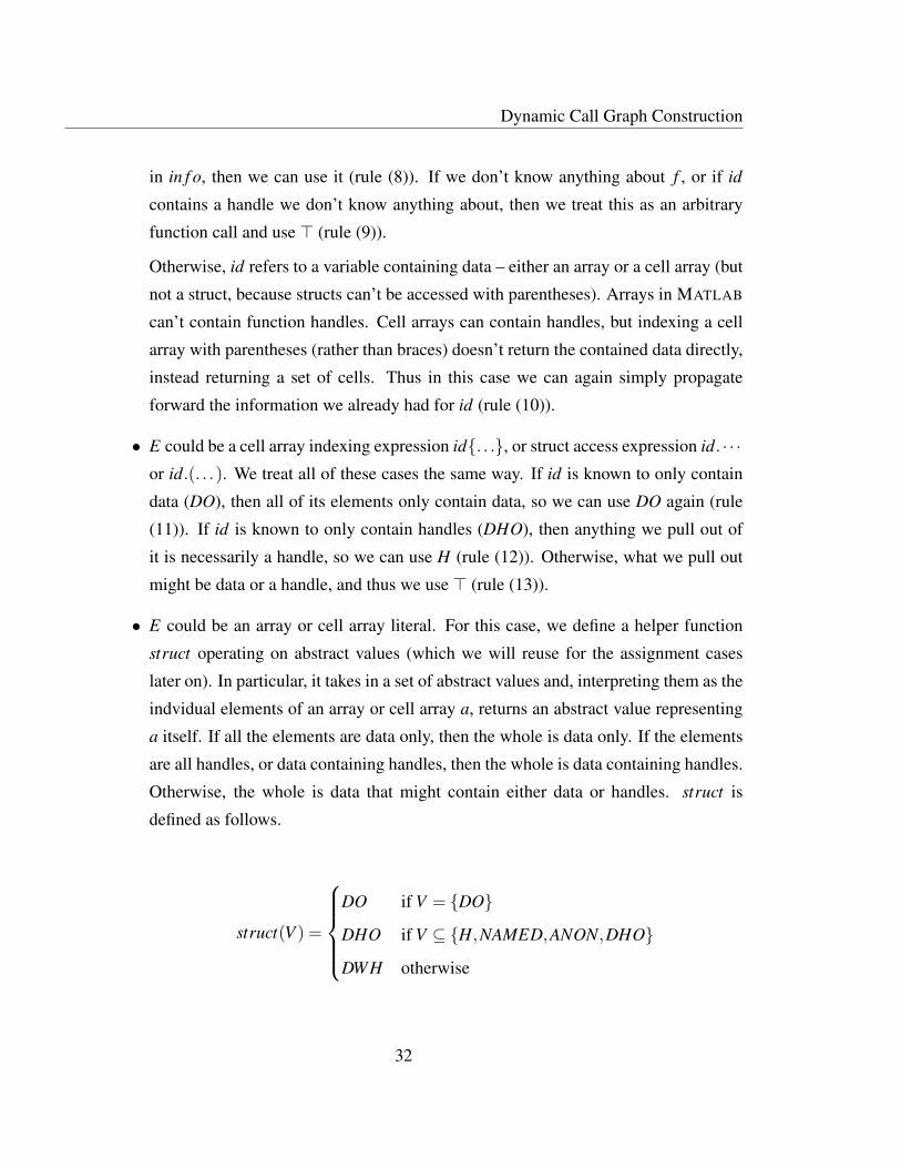
• E could be an array or cell array literal. For this case, we define a helper function
struct operating on abstract values (which we will reuse for the assignment cases
later on). In particular, it takes in a set of abstract values and, interpreting them as the
indvidual elements of an array or cell array a, returns an abstract value representing
a itself. If all the elements are data only, then the whole is data only. If the elements
are all handles, or data containing handles, then the whole is data containing handles.
Otherwise, the whole is data that might contain either data or handles. struct is
defined as follows.
struct(V ) =
DO if V = {DO}
DHO if V ⊆ {H,NAMED,ANON,DHO}
DWH otherwise
32
3.5. Minimizing overhead
For this case, we traverse the literal and compute the abstract values for each of the
constituent expressions, finally merging them together with struct (rule (14)).
• E could be any other expression. The ones we haven’t considered yet include arith-
metic and logical expressions, as well as numeric, string, colon and range literals.
All of these either are or operate on data only (rule (15)).
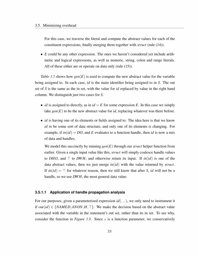
Table 3.5 shows how gen(E) is used to compute the new abstract value for the variable
being assigned to. In each case, id is the main identifier being assigned to in S. The out
set of S is the same as the in set, with the value for id replaced by value in the right hand
column. We distinguish just two cases for S.
• id is assigned to directly, as in id = E for some expression E. In this case we simply
take gen(E) to be the new abstract value for id, replacing whatever was there before.
• id is having one of its elements or fields assigned to. The idea here is that we know
id to be some sort of data structure, and only one of its elements is changing. For
example, if in(id) = DO, and E evaluates to a function handle, then id is now a mix
of data and handles.
We model this succinctly by running gen(E) through our struct helper function from
earlier. Given a single input value like this, struct will simply coalesce handle values
to DHO, and ⊤ to DWH, and otherwise return its input. If in(id) is one of the
data abstract values, then we just merge in(id) with the value returned by struct.
If in(id) = ⊤ for whatever reason, then we still know that after S, id will not be a
handle, so we use DWH, the most general data value.
3.5.1.1 Application of handle propagation analysis
For our purposes, given a parameterized expression id(. . .), we only need to instrument it
if out(id) ∈ {NAMED,ANON,H,⊤}. We make the decision based on the abstract value
associated with the variable in the statement’s out set, rather than its in set. To see why,
consider the function in Figure 3.9. Since a is a function parameter, we conservatively
33

Dynamic Call Graph Construction
Assignment out(id)id = E gen(E)id. · · ·= E in(id)∨ struct({gen(E)}) if in(id) ∈ {DWH,DHO,DO}id{. . .}= E DWH otherwiseid.(. . .) = E
id(. . .) = E
Table 3.5 Handle propagation analysis rules for assignments.
assign it the value ⊤. Once it is assigned to on line 3, it gets the value DWH, so we would
know not to instrument it, but before that statement, its value is still ⊤, so we would have
to instrument it. If a were a handle, however, then the assignment on line 3 would cause a
runtime error. By using the value in the out set, we can avoid over instrumenting in these
cases.
1 function f(a)
2 for i = 4:1000
3 a(i) = a(i-1) + a(i-2) + a(i-3);
4 end
5 end
Figure 3.9 A code snippet where a variable is used and assigned to in the same statement.
The "+ Prop" column in Table 3.2 shows how many expressions remain instrumented
with this enhancement applied, and the corresponding column in Table 3.3 shows the per-
formance of the instrumented code as a slowdown relative to the original uninstrumented
code. In general the analysis is very effective, weeding out many array accesses, and lead-
ing to big performance boosts; the capr benchmark, for example, runs nearly an order of
magnitude faster, going from a 1578x slowdown in the naive version to a 293x slowdown.
3.5.2 Avoiding builtin call instrumentation
MATLAB code tends to be fraught with calls to builtin functions, and instrumenting these
won’t give much benefit, since we don’t have access to their source code. However, because
MATLAB builtin functions can be shadowed by user-defined functions with the same name,
34
3.5. Minimizing overhead
or specialized via the mechanism described in Sec. 3.1, we can’t necessarily tell statically
whether a given function call is a call to a builtin function. Because of this, the naive
instrumentation goes ahead and instruments every function call, even if it likely is a call to
a builtin.
While we can’t statically determine the target of a function call to check whether it’s
a builtin, we can examine the application’s code, as well as any library code it depends
on, in order to gather a list A of user-defined functions whose names conflict with builtin
functions. In MATLAB, a function’s name is the name of the file it’s defined in (less the
extension), so this is just a simple filesystem traversal. Then, during instrumentation, when
we encounter a potential call to a builtin function, we check whether the name of the func-
tion appears in A. If it doesn’t, then we can safely avoid instrumenting the call. One
assumption here is that we have access to all the code the user is apt to run; this is not un-
reasonable, given that the user is requesting a call graph, and so is likely willing to provide
all the relevant code.
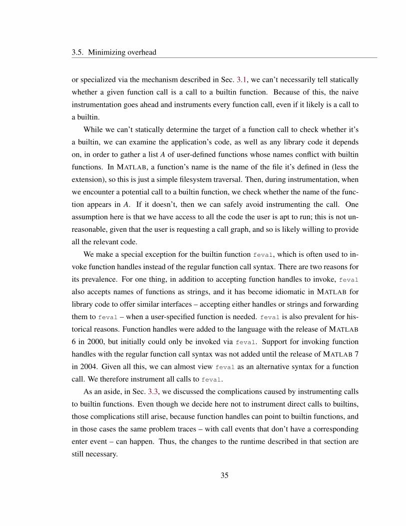
We make a special exception for the builtin function feval, which is often used to in-
voke function handles instead of the regular function call syntax. There are two reasons for
its prevalence. For one thing, in addition to accepting function handles to invoke, feval
also accepts names of functions as strings, and it has become idiomatic in MATLAB for
library code to offer similar interfaces – accepting either handles or strings and forwarding
them to feval – when a user-specified function is needed. feval is also prevalent for his-
torical reasons. Function handles were added to the language with the release of MATLAB
6 in 2000, but initially could only be invoked via feval. Support for invoking function
handles with the regular function call syntax was not added until the release of MATLAB 7
in 2004. Given all this, we can almost view feval as an alternative syntax for a function
call. We therefore instrument all calls to feval.
As an aside, in Sec. 3.3, we discussed the complications caused by instrumenting calls
to builtin functions. Even though we decide here not to instrument direct calls to builtins,
those complications still arise, because function handles can point to builtin functions, and
in those cases the same problem traces – with call events that don’t have a corresponding
enter event – can happen. Thus, the changes to the runtime described in that section are
still necessary.
35

Dynamic Call Graph Construction
The "- Builtins" column in Table 3.2 shows how many expressions remain instrumented
with this enhancement applied (in addition to the handle propagation analysis described in
the previous section) and the corresponding column in Table 3.3 shows the performance
of the instrumented code as a slowdown relative to the original uninstrumented code. The
effect of this optimizations depends on how heavily the benchmark relied on builtin func-
tions, but it is in general very effective, in many cases (e.g. dich, diff) reducing the overhead
to near 0.
3.5.3 Checking type of function arguments at runtime
Our instrumentation speculatively wraps each variable access in a function call in case the
variable is a function handle. A runtime check to determine whether it is occurs inside this
auxiliary function. This simplifies the transformation, but is clearly wasteful if the variable
turns out to be a plain array variable, especially if the variable is accessed more than once.
Since MATLAB is used a lot for numerical computations, MATLAB code tends to be heavy
on loops, such that array variables are often accessed repeatedly, magnifying the overhead.
Intuitively, we should be able to check the type of a given variable only once, and avoid
instrumenting accesses to it at all if it’s not a function handle.
However, this presents a complication in terms of implementation complexity. Wrap-
ping each variable access in a function call is a very simple transformation to make, as it
just involves replacing an expression AST node with another. If we start introducing con-
ditionals, the transformation becomes a lot more intrusive, since MATLAB does not support
any kind of conditional expression (such as the ternary ?: operator in C-based languages),
only conditional statements. Thus, inserting checks at the right places while preserving the
order of operations requires destructuring the code into a kind of three-address form.
The handle propagation analysis is precise enough in practice if we restrict ourselves
to a single function – a lot of the imprecision occurs when arrays are passed around as
function parameters. As a simple middle ground, we create two instrumented versions of
each function. In the first version (S for slow), we seed the handle propagation analysis
with the conservative assumption that any of the function parameters might be a function
handle (this is the same assumption we’ve been using thus far). In the second (F for fast),
36

3.5. Minimizing overhead
we seed it with the assumption that all of the function parameters are definitely just plain
data arrays. We then instrument both versions independently.
If both versions are the same, then there’s nothing to do. Otherwise, we replace the
body of the function with an if statement, with S as the then branch, and F as the else
branch. The condition checks at runtime, for each input parameter p with at least one use
instrumented in S, whether p is a function handle (using the MATLAB builtin function isa).
The "+ Checks" column in Table 3.2 shows how many expressions remain instrumented
along the fast path where the check reveals there are actually no handles, and the corre-
sponding columns in Table 3.3 shows the performance of the instrumented code with these
and all previous enhancements applied. For our more typical MATLAB benchmarks that
are heavy on array operations, this drastically reduces the overhead. For the benchmarks
that do use function handles, the effect on performance is predictably negligible.
3.5.4 Optimized runtime functions
The optimizations described thus far aim to reduce the number of expressions requiring
instrumentation. This helps tremendously on our numerical benchmarks, where the call
graphs are actually empty, or contain a single edge linking a call from the benchmark’s
driver function to the benchmark itself; in these cases, we can reduce the overhead to be
negligible. For those expressions where instrumentation is actually needed, however, we
also investigate the runtime overhead associated with each function call.
After some profiling on a long-running benchmark, we identify the following bottle-
necks.
• Our runtime uses the fprintf functions to log call and enter events to a log file. It
turns out that by default, MATLAB’s implementation of fprintf flushes the output
buffer each time the function is called, so that each of these calls is actually hitting
the filesystem. For builtin functions, this happens three times per call.
In addition to the usual ’w’ and ’a’ writing modes, MATLAB’s fopen function also
accepts ’W’ and ’A’, which behave similarly to their lowercase counterparts, ex-
cept that the output buffer is not flushed until it either reaches capacity or the file is
37
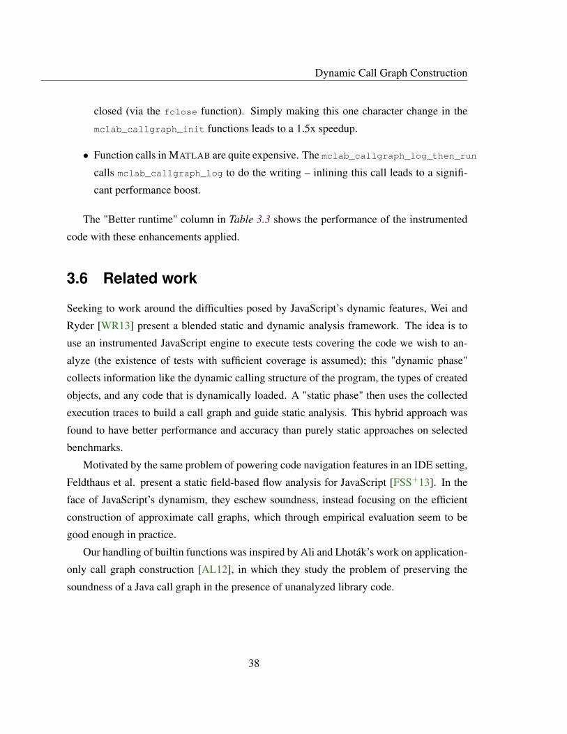
Dynamic Call Graph Construction
closed (via the fclose function). Simply making this one character change in the
mclab_callgraph_init functions leads to a 1.5x speedup.
• Function calls in MATLAB are quite expensive. The mclab_callgraph_log_then_run
calls mclab_callgraph_log to do the writing – inlining this call leads to a signifi-
cant performance boost.
The "Better runtime" column in Table 3.3 shows the performance of the instrumented
code with these enhancements applied.
3.6 Related work
Seeking to work around the difficulties posed by JavaScript’s dynamic features, Wei and
Ryder [WR13] present a blended static and dynamic analysis framework. The idea is to
use an instrumented JavaScript engine to execute tests covering the code we wish to an-
alyze (the existence of tests with sufficient coverage is assumed); this "dynamic phase"
collects information like the dynamic calling structure of the program, the types of created
objects, and any code that is dynamically loaded. A "static phase" then uses the collected
execution traces to build a call graph and guide static analysis. This hybrid approach was
found to have better performance and accuracy than purely static approaches on selected
benchmarks.
Motivated by the same problem of powering code navigation features in an IDE setting,
Feldthaus et al. present a static field-based flow analysis for JavaScript [FSS+13]. In the
face of JavaScript’s dynamism, they eschew soundness, instead focusing on the efficient
construction of approximate call graphs, which through empirical evaluation seem to be
good enough in practice.
Our handling of builtin functions was inspired by Ali and Lhoták’s work on application-
only call graph construction [AL12], in which they study the problem of preserving the
soundness of a Java call graph in the presence of unanalyzed library code.
38
Chapter 4
Layout-Preserving Refactorings
A refactoring is a code transformation that changes the structure of the code while
preserving its semantics, and can often naturally be thought of as a transformation over
the structure of an abstract syntax tree. However, from the perspective of a programmer
using a refactoring tool, a refactoring is ultimately a textual transformation. It is impor-
tant to reconcile these two conceptions of refactorings; purely working in terms of ASTs,
while technically correct from a semantics perspective, is apt to lose a lot of information
about the textual layout of the code, while purely working in terms of text is apt to make
implementations of individual refactorings very brittle, hard to reason about, and hard to
maintain.
In this chapter, we present our approach to the problem of implementing layout pre-
serving refactorings. We allow refactorings to be implemented in terms of a minimalist
tree transformation API, which hides the mechanics of layout preservation. As refactoring
writers specify tree-level changes, minimal text-level changes are transparently computed
from them. This simplifies the implementations of individual refactorings, allowing them
to remain oblivious to the program text and to operate at a higher level of abstraction,
without compromising their practicality for end-users.
39
Layout-Preserving Refactorings
4.1 Motivation
Setting aside questions of semantics preservation, a refactoring is most naturally thought of
as a transformation on abstract syntax trees. For instance, a refactoring like Extract Method
can be boiled down to high-level steps like these:
1. Synthesize a new function with the provided name
2. Move the selected sequence of statements from the target function to the new function
3. For each variable which is live at the input of the new function, add a corresponding
input parameter to the function (or possibly a global variable declaration)
4. For each variable which is live at the end of the new function, add a corresponding
output parameter to the function
5. Synthesize a new function call with the appropriate number of input and output ar-
guments
6. Insert this function call in the target function, at the position of the original sequence
of statements
These steps are agnostic to program text. Given this, a natural structure for a refactoring
tool consists of parsing code, then performing transformations on its AST, and then pretty
printing the transformed AST to retrieve source code to present to the programmer. Many
refactoring tools – particularly ones developed for research purposes, where practicality is
often a non-goal – operate this way.
The problem with such approaches is that by construction the AST does not contain
enough information to accurately reconstruct the input source code. Typically among the
casualties are indentation and other whitespace, along with comments and syntactic sugar.
Figure 4.1 shows a MATLAB program and the result of parsing and then pretty-printing
it using the McLAB toolkit. The two programs are behaviorally equivalent, but contain
many syntactic differences. The comment associated with the cube function has moved
below the header. The four-space indentation has been changed to two-space indentation.
40

4.1. Motivation
% cube takes a number x and returns
its cube.
function y = cube(x)
% This is a nested function that
computes the square of a
value.
function v = square(u)
v = u * u;
end
y = x * square(x);
end
function [y] = cube(x)
% cube takes a number x and
returns its cube.
% This is a nested function that
computes the square of a value.
y = (x * square(x));
function [v] = square(u)
v = (u * u);
end
end
Figure 4.1 An example of the lossy parsing and unparsing roundtrip.
Each binary expression has been wrapped in parentheses. The output parameters have been
wrapped in square brackets. The nested function square has been moved – in MATLAB,
nested functions have the same scope irrespective of where they are declared, so during
parsing they are all moved to the end of their enclosing functions as a simplification step.
Users of an automated refactoring tool are unlikely to be accepting of such invasive
changes to a program’s text. As such, it is important for any refactoring tool to be aware of
the layout of the program when performing refactorings. For a given AST transformation,
it should endeavor to perform the minimal textual changes needed to reflect the transfor-
mation in the program text. In particular, unaffected portions of the program should not
undergo any textual changes.
Despite this, it is still convenient to express refactorings as tree transformations. Refac-
torings would be much harder to implement and maintain if they had to be expressed as
textual transformations, or as a mixture of tree and text transformations that had to be kept
in sync.
Our goal is to be able to implement refactorings purely as tree transformations, and to
have minimal textual changes automatically computed from them. In order to accomplish
this, we introduce a simple transformation API, which exposes a small set of tree manipula-
tion operations. Instead of directly manipulating AST nodes, refactorings are implemented
in terms of this API. Behind the scenes, the implementation of the API includes logic that
keeps track of the input program text in addition to the AST, and keeps the two in sync.
41
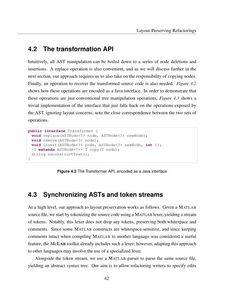
Layout-Preserving Refactorings
4.2 The transformation API
Intuitively, all AST manipulation can be boiled down to a series of node deletions and
insertions. A replace operation is also convenient, and as we will discuss further in the
next section, our approach requires us to also take on the responsibility of copying nodes.
Finally, an operation to recover the transformed source code is also needed. Figure 4.2
shows how these operations are encoded as a Java interface. In order to demonstrate that
these operations are just conventional tree manipulation operations, Figure 4.3 shows a
trivial implementation of the interface that just falls back on the operations exposed by
the AST, ignoring layout concerns; note the close correspondence between the two sets of
operations.
public interface Transformer {
void replace(ASTNode<?> node, ASTNode<?> newNode);
void remove(ASTNode<?> node);
void insert(ASTNode<?> node, ASTNode<?> newNode, int i);
<T extends ASTNode<?>> T copy(T node);
String reconstructText();
}
Figure 4.2 The Transformer API, encoded as a Java interface
4.3 Synchronizing ASTs and token streams
At a high level, our approach to layout preservation works as follows. Given a MATLAB
source file, we start by tokenizing the source code using a MATLAB lexer, yielding a stream
of tokens. Notably, this lexer does not drop any tokens, preserving both whitespace and
comments. Since some MATLAB constructs are whitespace-sensitive, and since keeping
comments intact when compiling MATLAB to another language was considered a useful
feature, the McLAB toolkit already includes such a lexer; however, adapting this approach
to other languages may involve the use of a specialized lexer.
Alongside the token stream, we use a MATLAB parser to parse the same source file,
yielding an abstract syntax tree. Our aim is to allow refactoring writers to specify edits
42
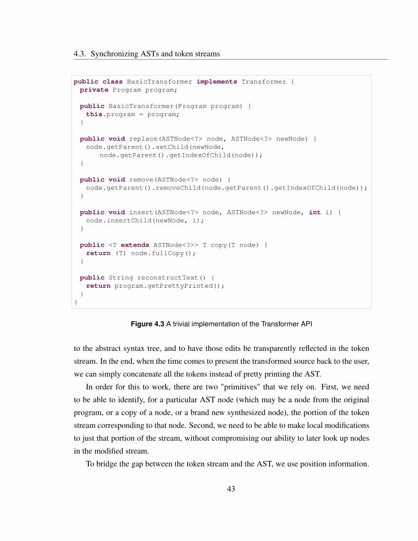
4.3. Synchronizing ASTs and token streams
public class BasicTransformer implements Transformer {
private Program program;
public BasicTransformer(Program program) {
this.program = program;
}
public void replace(ASTNode<?> node, ASTNode<?> newNode) {
node.getParent().setChild(newNode,
node.getParent().getIndexOfChild(node));
}
public void remove(ASTNode<?> node) {
node.getParent().removeChild(node.getParent().getIndexOfChild(node));
}
public void insert(ASTNode<?> node, ASTNode<?> newNode, int i) {
node.insertChild(newNode, i);
}
public <T extends ASTNode<?>> T copy(T node) {
return (T) node.fullCopy();
}
public String reconstructText() {
return program.getPrettyPrinted();
}
}
Figure 4.3 A trivial implementation of the Transformer API
to the abstract syntax tree, and to have those edits be transparently reflected in the token
stream. In the end, when the time comes to present the transformed source back to the user,
we can simply concatenate all the tokens instead of pretty printing the AST.
In order for this to work, there are two "primitives" that we rely on. First, we need
to be able to identify, for a particular AST node (which may be a node from the original
program, or a copy of a node, or a brand new synthesized node), the portion of the token
stream corresponding to that node. Second, we need to be able to make local modifications
to just that portion of the stream, without compromising our ability to later look up nodes
in the modified stream.
To bridge the gap between the token stream and the AST, we use position information.
43
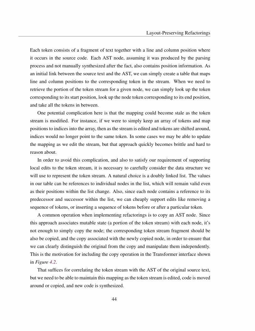
Layout-Preserving Refactorings
Each token consists of a fragment of text together with a line and column position where
it occurs in the source code. Each AST node, assuming it was produced by the parsing
process and not manually synthesized after the fact, also contains position information. As
an initial link between the source text and the AST, we can simply create a table that maps
line and column positions to the corresponding token in the stream. When we need to
retrieve the portion of the token stream for a given node, we can simply look up the token
corresponding to its start position, look up the node token corresponding to its end position,
and take all the tokens in between.
One potential complication here is that the mapping could become stale as the token
stream is modified. For instance, if we were to simply keep an array of tokens and map
positions to indices into the array, then as the stream is edited and tokens are shifted around,
indices would no longer point to the same token. In some cases we may be able to update
the mapping as we edit the stream, but that approach quickly becomes brittle and hard to
reason about.
In order to avoid this complication, and also to satisfy our requirement of supporting
local edits to the token stream, it is necessary to carefully consider the data structure we
will use to represent the token stream. A natural choice is a doubly linked list. The values
in our table can be references to individual nodes in the list, which will remain valid even
as their positions within the list change. Also, since each node contains a reference to its
predecessor and successor within the list, we can cheaply support edits like removing a
sequence of tokens, or inserting a sequence of tokens before or after a particular token.
A common operation when implementing refactorings is to copy an AST node. Since
this approach associates mutable state (a portion of the token stream) with each node, it’s
not enough to simply copy the node; the corresponding token stream fragment should be
also be copied, and the copy associated with the newly copied node, in order to ensure that
we can clearly distinguish the original from the copy and manipulate them independently.
This is the motivation for including the copy operation in the Transformer interface shown
in Figure 4.2.
That suffices for correlating the token stream with the AST of the original source text,
but we need to be able to maintain this mapping as the token stream is edited, code is moved
around or copied, and new code is synthesized.
44
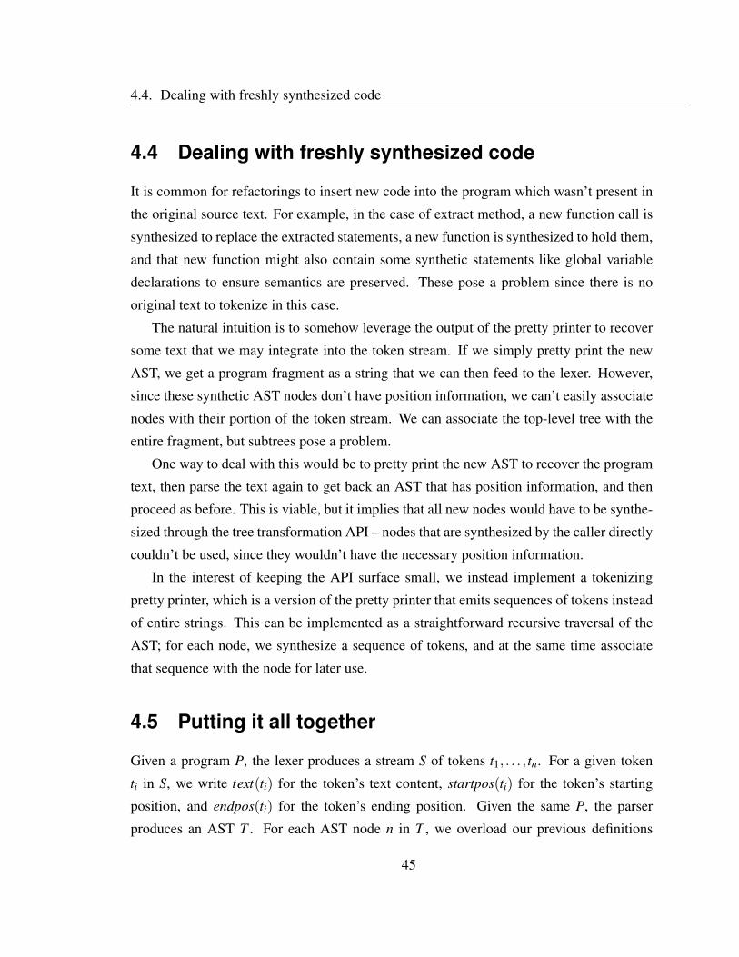
4.4. Dealing with freshly synthesized code
4.4 Dealing with freshly synthesized code
It is common for refactorings to insert new code into the program which wasn’t present in
the original source text. For example, in the case of extract method, a new function call is
synthesized to replace the extracted statements, a new function is synthesized to hold them,
and that new function might also contain some synthetic statements like global variable
declarations to ensure semantics are preserved. These pose a problem since there is no
original text to tokenize in this case.
The natural intuition is to somehow leverage the output of the pretty printer to recover
some text that we may integrate into the token stream. If we simply pretty print the new
AST, we get a program fragment as a string that we can then feed to the lexer. However,
since these synthetic AST nodes don’t have position information, we can’t easily associate
nodes with their portion of the token stream. We can associate the top-level tree with the
entire fragment, but subtrees pose a problem.
One way to deal with this would be to pretty print the new AST to recover the program
text, then parse the text again to get back an AST that has position information, and then
proceed as before. This is viable, but it implies that all new nodes would have to be synthe-
sized through the tree transformation API – nodes that are synthesized by the caller directly
couldn’t be used, since they wouldn’t have the necessary position information.
In the interest of keeping the API surface small, we instead implement a tokenizing
pretty printer, which is a version of the pretty printer that emits sequences of tokens instead
of entire strings. This can be implemented as a straightforward recursive traversal of the
AST; for each node, we synthesize a sequence of tokens, and at the same time associate
that sequence with the node for later use.
4.5 Putting it all together
Given a program P, the lexer produces a stream S of tokens t1, . . . , tn. For a given token
ti in S, we write text(ti) for the token’s text content, startpos(ti) for the token’s starting
position, and endpos(ti) for the token’s ending position. Given the same P, the parser
produces an AST T . For each AST node n in T , we overload our previous definitions
45

Layout-Preserving Refactorings
and write startpos(n) for the node’s starting position, and endpos(n) for the node’s ending
position, which are the same as the starting and ending positions of the first and last tokens
corresponding to n, respectively. We take all of these as inputs; these are conventionally
provided by a typical lexer and parser.
We start by creating a doubly linked list L with a node for each token in the token
stream. We write head(L) and tail(L) for the head and tail nodes of L, respectively. Given
a node n, we write token(n) for the token associated with n, prev(n) for its predecessor
node in L, and next(n) for its successor node in L. We then define a mapping P from
source positions to nodes in L; for each node n in L, we map both startpos(token(n)) and
endpos(token(n)) to n.
A token stream fragment f = 〈start( f ),end( f )〉 is a pair of nodes in L: a starting node
start( f ) and an ending node end( f ). Given an AST node n in T , we ultimately need
to be able to retrieve (or synthesize) a corresponding token stream fragment. For a node
n occurring in the original AST produced by the parser, the corresponding token stream
fragment is 〈P[startpos(n)],P[endpos(n)]〉, but as alluded to in the previous sections, this
won’t be accurate when dealing with synthetic nodes, or copies of nodes. To handle these,
we allow a node’s token stream fragment to be set explicitly, skipping the lookup in P.
This facility is used by the tokenizing pretty printer, and in the implementation of the copy
operation. We write f ragment(n) to retrieve the token stream fragment associated with
node n, if any.
Now when it comes to getting at a token stream fragment corresponding to a given AST
node n, we distinguish between the following cases.
1. n is a node from the original program, existing in the original AST produced by the
parser. In that case, the corresponding fragment is just 〈P[startpos(n)],P[endpos(n)]〉.
2. n is a synthetic node we’re seeing for the first time. In that case, we invoke the
tokenizing pretty printer on n, which will output another doubly linked list L′. Now
the corresponding fragment is 〈head(L′), tail(L′)〉.
3. n is a synthetic node we’ve seen before. In that case, the corresponding fragment is
f ragment(n).
46

4.6. Heuristics for handling indentation and comments
4. n is a copy of another node. In this case, the corresponding fragment is again
f ragment(n).
4.6 Heuristics for handling indentation and comments
Our approach of correlating AST nodes with fragments of the original program text and
performing local edits to the token stream lets us easily preserve the layout of the unaffected
portions of the code, as well as the internal layout of the affected portions. However, care
must still be taken when dealing with code at the boundary between affected and unaffected.
For instance, when inserting a statement in the body of a deeply nested control structure,
we should pick an appropriate amount of indentation to match the surrounding code – but
the program indentation might be inconsistent, or there might not be any surrounding code
in a particular file. Statements can also have comments associated with them, and ideally
these should be moved alongside their subjects – but since comments are largely free-form,
there is no easy way to identify which comments are associated with a given statement. In
both cases, we rely on heuristics to try and do something sensible.
4.6.1 Indentation
When moving statements or functions, we attempt to match the surrounding indentation.
Given a simple statement node n, we compute its indentation level by taking start( f ragment(n))
and searching backwards along its predecessor nodes until a non-whitespace or newline to-
ken t is reached. Then the token stream fragment corresponding to the indentation is
〈next(t), prev(start( f ragment(n)))〉 (which is possibly empty). For a multiline construct
like a function or a loop, we compute the indentation of each line and take the common
prefix. When inserting a node, we try to guess the appropriate amount of indentation to
insert by applying the following heuristic.
1. Special case: if we’re inserting a statement between two semicolon or comma sepa-
rated statements on the same line, then there’s no indentation to add.
2. Otherwise, look for a predecessor or successor AST node and copy its indentation.
47

Layout-Preserving Refactorings
function_call() % This comment spans multiple lines
another_call() % and lies adjacent to many statements
some_core_code() % but should be considered associated with
% the first function call.
Figure 4.4 An illustration of wacky commenting practices.
3. Otherwise, look for a statement or function list elsewhere in the file, and copy the
indentation of the first node there.
4. Otherwise, there is nothing to go on – a more sophisticated approach might inspect
different files in the project, but each token stream is tied to a single file – so we fall
back to an arbitrary (potentially configurable) default of four spaces.
4.6.2 Comments
In order to represent an association between a comment and a language construct, we sim-
ply extend the token stream fragment associated with the construct to include the comment.
Note that this implies the portion of the program text including the construct and the com-
ment must be contiguous, which might be problematic; for example, consider the (artificial)
case in Figure 4.4, where multiple aligned inline comments are meant to be associated with
the first statement. We choose not to handle such cases; at the least, it would dispropor-
tionately complicate the implementation, as each node might have several disparate token
stream fragments associated with it.
Comments can be associated with any kind of language construct, including functions,
scripts, classes, methods, statements and even individual expressions. Comments associ-
ated with a node are also implicitly associated with its ancestor nodes, so that, for instance,
moving a function call also moves any comments associated with its arguments. In each
case, when an operation is performed on a node, we inspect the surrounding code to gather
any associated comments. Given a node, our heuristic is as follows.
1. For a statement or an expression, we include the trailing inline comment, if any.
Given the node n, we take end( f ragment(n)), which is a node in L, and search
forwards along its successor nodes, skipping over any space or tab (but not newline)
48
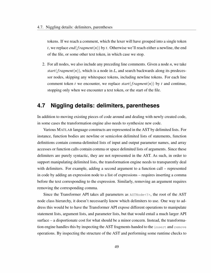
4.7. Niggling details: delimiters, parentheses
tokens. If we reach a comment, which the lexer will have grouped into a single token
t, we replace end( f ragment(n)) by t. Otherwise we’ll reach either a newline, the end
of the file, or some other text token, in which case we stop.
2. For all nodes, we also include any preceding line comments. Given a node n, we take
start( f ragment(n)), which is a node in L, and search backwards along its predeces-
sor nodes, skipping any whitespace tokens, including newline tokens. For each line
comment token t we encounter, we replace start( f ragment(n)) by t and continue,
stopping only when we encounter a text token, or the start of the file.
4.7 Niggling details: delimiters, parentheses
In addition to moving existing pieces of code around and dealing with newly created code,
in some cases the transformation engine also needs to synthesize new code.
Various MATLAB language constructs are represented in the AST by delimited lists. For
instance, function bodies are newline or semicolon delimited lists of statements, function
definitions contain comma-delimited lists of input and output parameter names, and array
accesses or function calls contain comma or space delimited lists of arguments. Since these
delimiters are purely syntactic, they are not represented in the AST. As such, in order to
support manipulating delimited lists, the transformation engine needs to transparently deal
with delimiters. For example, adding a second argument to a function call – represented
in code by adding an expression node to a list of expressions – requires inserting a comma
before the text corresponding to the expression. Similarly, removing an argument requires
removing the corresponding comma.
Since the Transformer API takes all parameters as ASTNode<?>, the root of the AST
node class hierarchy, it doesn’t necessarily know which delimiters to use. One way to ad-
dress this would be to have the Transformer API expose different operations to manipulate
statement lists, argument lists, and parameter lists, but that would entail a much larger API
surface – a disportionate cost for what should be a minor concern. Instead, the transforma-
tion engine handles this by inspecting the AST fragments handed to the insert and remove
operations. By inspecting the structure of the AST and performing some runtime checks to
49
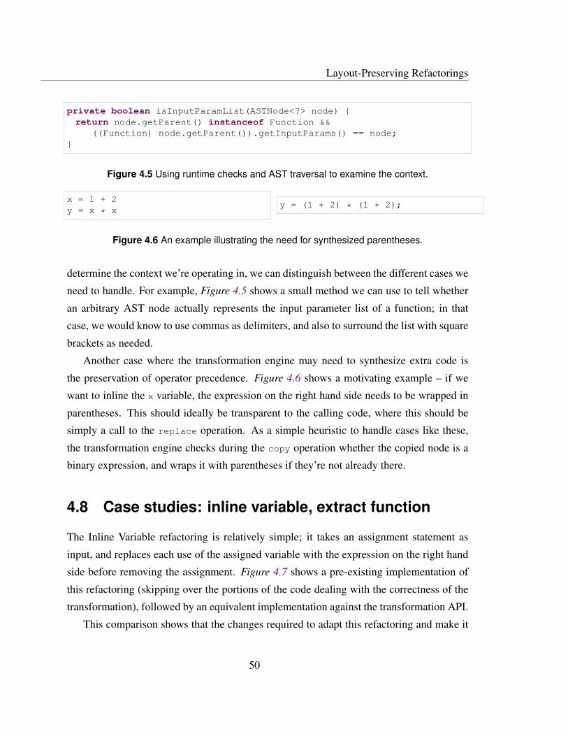
Layout-Preserving Refactorings
private boolean isInputParamList(ASTNode<?> node) {
return node.getParent() instanceof Function &&
((Function) node.getParent()).getInputParams() == node;
}
Figure 4.5 Using runtime checks and AST traversal to examine the context.
x = 1 + 2
y = x * xy = (1 + 2) * (1 + 2);
Figure 4.6 An example illustrating the need for synthesized parentheses.
determine the context we’re operating in, we can distinguish between the different cases we
need to handle. For example, Figure 4.5 shows a small method we can use to tell whether
an arbitrary AST node actually represents the input parameter list of a function; in that
case, we would know to use commas as delimiters, and also to surround the list with square
brackets as needed.
Another case where the transformation engine may need to synthesize extra code is
the preservation of operator precedence. Figure 4.6 shows a motivating example – if we
want to inline the x variable, the expression on the right hand side needs to be wrapped in
parentheses. This should ideally be transparent to the calling code, where this should be
simply a call to the replace operation. As a simple heuristic to handle cases like these,
the transformation engine checks during the copy operation whether the copied node is a
binary expression, and wraps it with parentheses if they’re not already there.
4.8 Case studies: inline variable, extract function
The Inline Variable refactoring is relatively simple; it takes an assignment statement as
input, and replaces each use of the assigned variable with the expression on the right hand
side before removing the assignment. Figure 4.7 shows a pre-existing implementation of
this refactoring (skipping over the portions of the code dealing with the correctness of the
transformation), followed by an equivalent implementation against the transformation API.
This comparison shows that the changes required to adapt this refactoring and make it
50
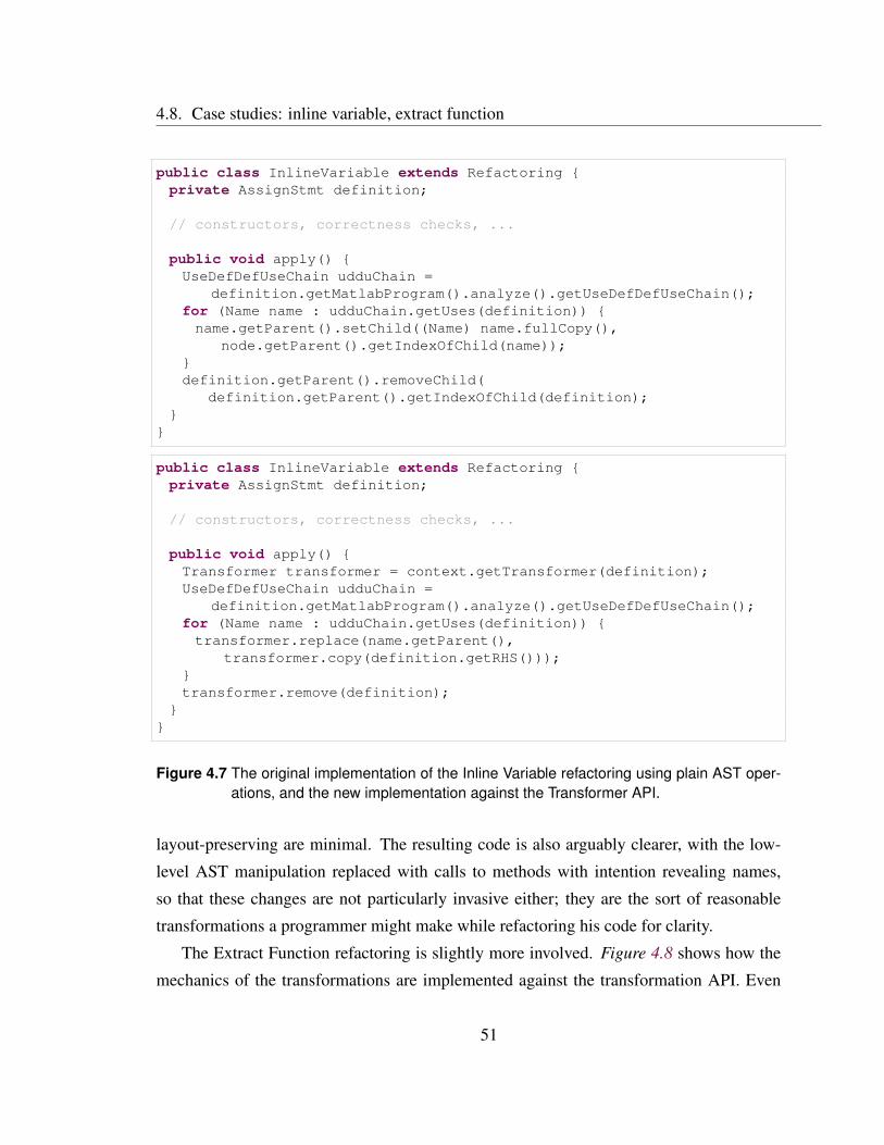
4.8. Case studies: inline variable, extract function
public class InlineVariable extends Refactoring {
private AssignStmt definition;
// constructors, correctness checks, ...
public void apply() {
UseDefDefUseChain udduChain =
definition.getMatlabProgram().analyze().getUseDefDefUseChain();
for (Name name : udduChain.getUses(definition)) {
name.getParent().setChild((Name) name.fullCopy(),
node.getParent().getIndexOfChild(name));
}
definition.getParent().removeChild(
definition.getParent().getIndexOfChild(definition);
}
}
public class InlineVariable extends Refactoring {
private AssignStmt definition;
// constructors, correctness checks, ...
public void apply() {
Transformer transformer = context.getTransformer(definition);
UseDefDefUseChain udduChain =
definition.getMatlabProgram().analyze().getUseDefDefUseChain();
for (Name name : udduChain.getUses(definition)) {
transformer.replace(name.getParent(),
transformer.copy(definition.getRHS()));
}
transformer.remove(definition);
}
}
Figure 4.7 The original implementation of the Inline Variable refactoring using plain AST oper-
ations, and the new implementation against the Transformer API.
layout-preserving are minimal. The resulting code is also arguably clearer, with the low-
level AST manipulation replaced with calls to methods with intention revealing names,
so that these changes are not particularly invasive either; they are the sort of reasonable
transformations a programmer might make while refactoring his code for clarity.
The Extract Function refactoring is slightly more involved. Figure 4.8 shows how the
mechanics of the transformations are implemented against the transformation API. Even
51
Layout-Preserving Refactorings
though the refactoring moves AST nodes around, copies nodes, and mixes in synthetic
code with the original text, the code is completely oblivious to text, instead leaning on the
Transformer to do the heavy lifting.
4.9 Related work
4.9.1 HaRe
The work that most closely resembles ours is HaRe, a refactoring tool for Haskell [Li06].
It uses a similar approach of synchronizing an AST with a token stream; program analyses
are carried out using the AST, but program transformations are carried out on the token
stream alongside the AST, and source positions are used to bridge the two.
Rather than using a tokenizing pretty printer for synthesized code, the output of the
regular pretty printer is used, together with a scheme where the concatenated tokens are
re-lexed to obtain correct positions which are then used to update the position information
of existing AST nodes.
Similar heuristics for associating comments with program structures are also presented.
There are some extra constraints that apply for Haskell programs, as these can be writ-
ten in a layout-sensitive style where indentation is significant, so that care must be taken to
ensure that the new code is behaviorally equivalent to the original after it has gone through
the layout preservation machinery. To address this, an explicit "layout adjustment" algo-
rithm is presented which is run after each refactoring, adding or removing whitespace as
needed to restore the meaning of the input program.
The API exposed by HaRe for carrying out transformations is quite a bit larger than
ours, as each of adding code, removing code and updating existing code is handled by
a family of functions that deal with different AST node types – whereas, as described
in Sec. 4.2, one of our design goals was to minimize the API surface, so that existing
refactorings could be updated to be layout-preserving without much effort expended in
rewriting. This difference might just be a consequence of the underlying differences in
parsing tools and AST representations that our implementations are built on top of.
52
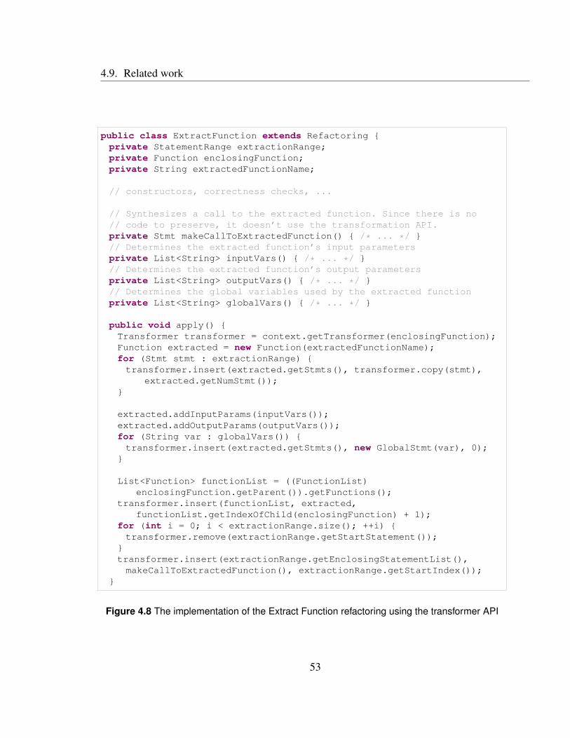
4.9. Related work
public class ExtractFunction extends Refactoring {
private StatementRange extractionRange;
private Function enclosingFunction;
private String extractedFunctionName;
// constructors, correctness checks, ...
// Synthesizes a call to the extracted function. Since there is no
// code to preserve, it doesn’t use the transformation API.
private Stmt makeCallToExtractedFunction() { /* ... */ }
// Determines the extracted function’s input parameters
private List<String> inputVars() { /* ... */ }
// Determines the extracted function’s output parameters
private List<String> outputVars() { /* ... */ }
// Determines the global variables used by the extracted function
private List<String> globalVars() { /* ... */ }
public void apply() {
Transformer transformer = context.getTransformer(enclosingFunction);
Function extracted = new Function(extractedFunctionName);
for (Stmt stmt : extractionRange) {
transformer.insert(extracted.getStmts(), transformer.copy(stmt),
extracted.getNumStmt());
}
extracted.addInputParams(inputVars());
extracted.addOutputParams(outputVars());
for (String var : globalVars()) {
transformer.insert(extracted.getStmts(), new GlobalStmt(var), 0);
}
List<Function> functionList = ((FunctionList)
enclosingFunction.getParent()).getFunctions();
transformer.insert(functionList, extracted,
functionList.getIndexOfChild(enclosingFunction) + 1);
for (int i = 0; i < extractionRange.size(); ++i) {
transformer.remove(extractionRange.getStartStatement());
}
transformer.insert(extractionRange.getEnclosingStatementList(),
makeCallToExtractedFunction(), extractionRange.getStartIndex());
}
Figure 4.8 The implementation of the Extract Function refactoring using the transformer API
53

Layout-Preserving Refactorings
4.9.2 Other approaches
De Jonge and Visser [dJV12] present an algorithm for layout preservation in refactoring
transformations. While the token stream is used to access the layout structure surrounding
a given AST node, it is not modified in parallel with the AST; instead, the source code is
reconstructed afterwards using a combination of the original program text, pretty printed
text, and the application of a tree differencing algorithm to detect insertions and deletions.
An attempt is made to formalize the problem and prove the algorithm correct within that
formalization; by contrast, we are largely describing an implemention.
Waddington and Yao [WY05] tackled the same problem, which they termed "the prob-
lem of style disruption", with Proteus, their refactoring tool for C and C++. Their approach
was to use a specialized AST called a "Literal-Layout AST (LL-AST)", where literals, to-
ken and whitespace nodes are interspersed alongside the regular nodes. Enhancing the AST
with layout information has also been the theme of a few other approaches to this problem
[KLN+09].
The Eclipse JDT contains infrastructure for modifying code at two levels – a lower-level
API for describing text manipulation primitives, and a higher-level AST rewriting API,
which accepts descriptions of changes to AST nodes and uses the text manipulation API to
try and perform the textual changes required to represent the AST changes. The approach is
similar to ours in spirit; one big difference is that since our approach is implemented largely
as a standalone tool, we rely solely on lexing and parsing as primitives, while Eclipse’s
implementation benefits from more sophisticated integration with a scriptable text editor.
54
Chapter 5
Survey of Dynamic Features
MATLAB supports many heavily dynamic features that are problematic for static anal-
ysis, and which at present are either ignored or rejected by different components of the
McLab toolkit. These include
• scripts, which have error prone scoping semantics compared to functions
• arbitrary dynamic code evaluation via eval
• dynamic function calls via feval
• dynamic workspace manipulation either by deleting variables via clear or clearvars
or assigning to them via assignin or evalin
• dynamic workspace inspection via exist, who or whos
• dynamic modification of the function lookup path via cd, path, addpath, rmpath
In this chapter, we examine each of these, giving a brief primer on their semantics
and investigating how frequently they occur, and common patterns in their usage. Similar
invstigations for other dynamic programming languages such as JavaScript [RHBV11] and
Ruby [FhDAF09] have shown that in practice, such dynamic features tend to be used in
very restricted ways which aren’t actually difficult to reason about statically, and we find
that the same holds for MATLAB.
55
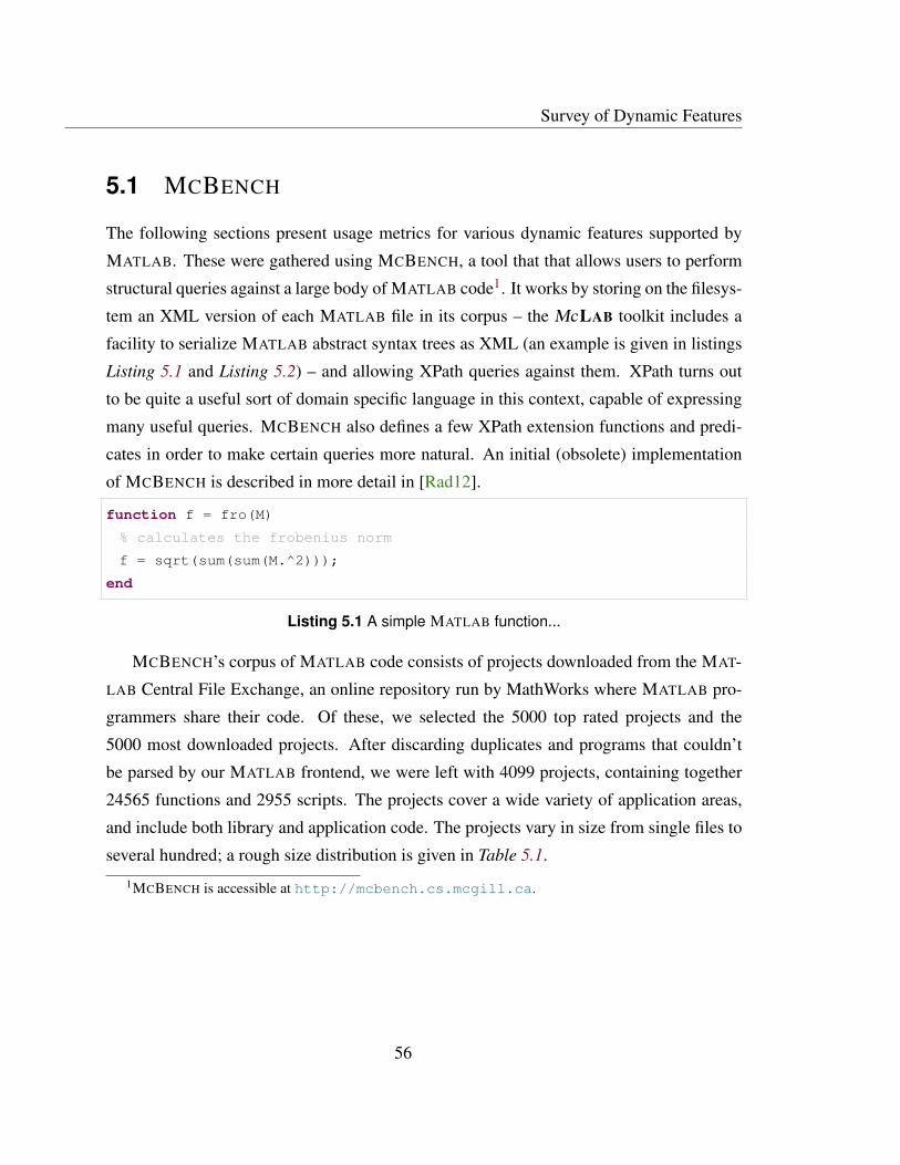
Survey of Dynamic Features
5.1 MCBENCH
The following sections present usage metrics for various dynamic features supported by
MATLAB. These were gathered using MCBENCH, a tool that that allows users to perform
structural queries against a large body of MATLAB code1. It works by storing on the filesys-
tem an XML version of each MATLAB file in its corpus – the McLAB toolkit includes a
facility to serialize MATLAB abstract syntax trees as XML (an example is given in listings
Listing 5.1 and Listing 5.2) – and allowing XPath queries against them. XPath turns out
to be quite a useful sort of domain specific language in this context, capable of expressing
many useful queries. MCBENCH also defines a few XPath extension functions and predi-
cates in order to make certain queries more natural. An initial (obsolete) implementation
of MCBENCH is described in more detail in [Rad12].
function f = fro(M)
% calculates the frobenius norm
f = sqrt(sum(sum(M.^2)));
end
Listing 5.1 A simple MATLAB function...
MCBENCH’s corpus of MATLAB code consists of projects downloaded from the MAT-
LAB Central File Exchange, an online repository run by MathWorks where MATLAB pro-
grammers share their code. Of these, we selected the 5000 top rated projects and the
5000 most downloaded projects. After discarding duplicates and programs that couldn’t
be parsed by our MATLAB frontend, we were left with 4099 projects, containing together
24565 functions and 2955 scripts. The projects cover a wide variety of application areas,
and include both library and application code. The projects vary in size from single files to
several hundred; a rough size distribution is given in Table 5.1.
1MCBENCH is accessible at http://mcbench.cs.mcgill.ca.
56
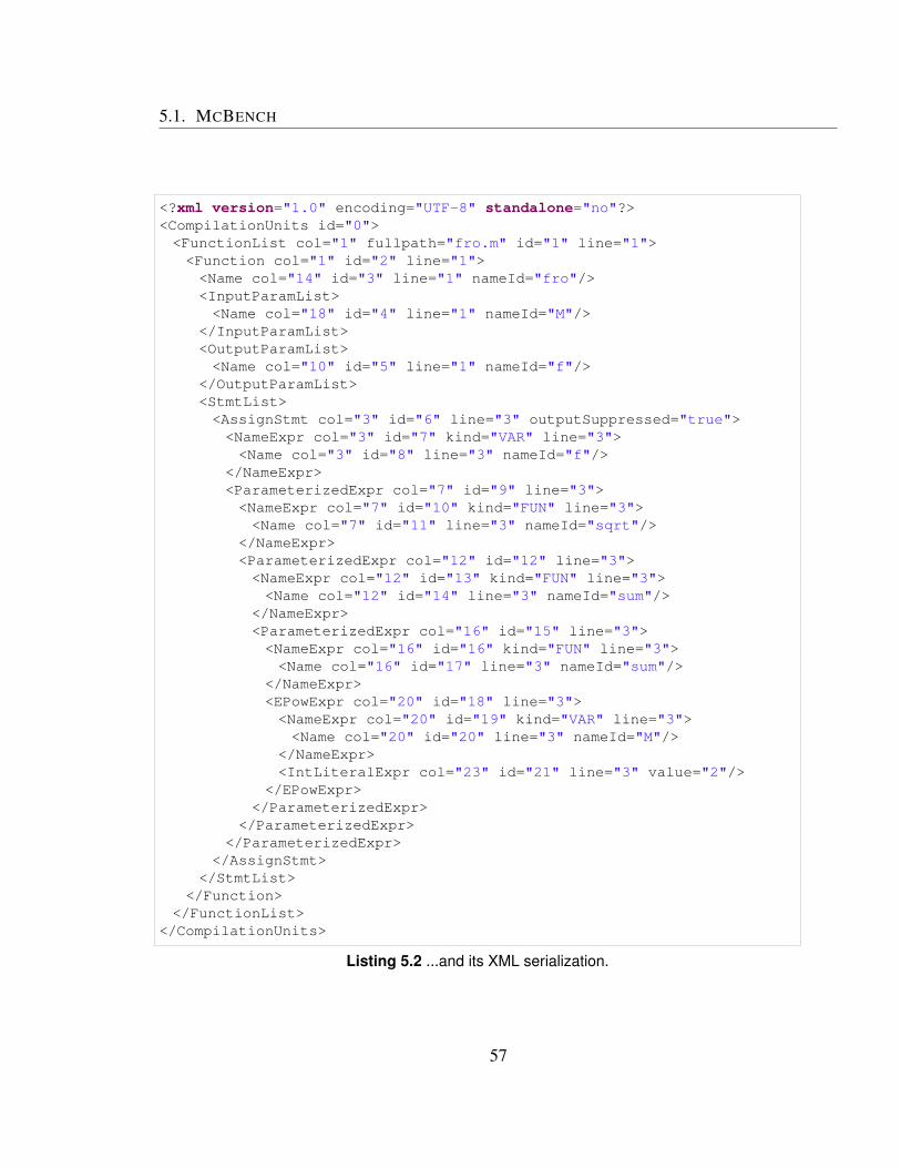
5.1. MCBENCH
<?xml version="1.0" encoding="UTF-8" standalone="no"?>
<CompilationUnits id="0">
<FunctionList col="1" fullpath="fro.m" id="1" line="1">
<Function col="1" id="2" line="1">
<Name col="14" id="3" line="1" nameId="fro"/>
<InputParamList>
<Name col="18" id="4" line="1" nameId="M"/>
</InputParamList>
<OutputParamList>
<Name col="10" id="5" line="1" nameId="f"/>
</OutputParamList>
<StmtList>
<AssignStmt col="3" id="6" line="3" outputSuppressed="true">
<NameExpr col="3" id="7" kind="VAR" line="3">
<Name col="3" id="8" line="3" nameId="f"/>
</NameExpr>
<ParameterizedExpr col="7" id="9" line="3">
<NameExpr col="7" id="10" kind="FUN" line="3">
<Name col="7" id="11" line="3" nameId="sqrt"/>
</NameExpr>
<ParameterizedExpr col="12" id="12" line="3">
<NameExpr col="12" id="13" kind="FUN" line="3">
<Name col="12" id="14" line="3" nameId="sum"/>
</NameExpr>
<ParameterizedExpr col="16" id="15" line="3">
<NameExpr col="16" id="16" kind="FUN" line="3">
<Name col="16" id="17" line="3" nameId="sum"/>
</NameExpr>
<EPowExpr col="20" id="18" line="3">
<NameExpr col="20" id="19" kind="VAR" line="3">
<Name col="20" id="20" line="3" nameId="M"/>
</NameExpr>
<IntLiteralExpr col="23" id="21" line="3" value="2"/>
</EPowExpr>
</ParameterizedExpr>
</ParameterizedExpr>
</ParameterizedExpr>
</AssignStmt>
</StmtList>
</Function>
</FunctionList>
</CompilationUnits>
Listing 5.2 ...and its XML serialization.
57
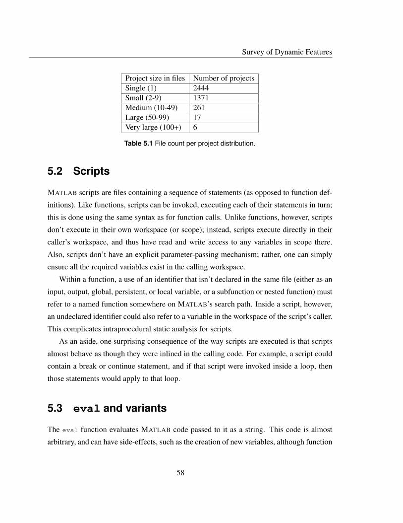
Survey of Dynamic Features
Project size in files Number of projectsSingle (1) 2444Small (2-9) 1371Medium (10-49) 261Large (50-99) 17Very large (100+) 6
Table 5.1 File count per project distribution.
5.2 Scripts
MATLAB scripts are files containing a sequence of statements (as opposed to function def-
initions). Like functions, scripts can be invoked, executing each of their statements in turn;
this is done using the same syntax as for function calls. Unlike functions, however, scripts
don’t execute in their own workspace (or scope); instead, scripts execute directly in their
caller’s workspace, and thus have read and write access to any variables in scope there.
Also, scripts don’t have an explicit parameter-passing mechanism; rather, one can simply
ensure all the required variables exist in the calling workspace.
Within a function, a use of an identifier that isn’t declared in the same file (either as an
input, output, global, persistent, or local variable, or a subfunction or nested function) must
refer to a named function somewhere on MATLAB’s search path. Inside a script, however,
an undeclared identifier could also refer to a variable in the workspace of the script’s caller.
This complicates intraprocedural static analysis for scripts.
As an aside, one surprising consequence of the way scripts are executed is that scripts
almost behave as though they were inlined in the calling code. For example, a script could
contain a break or continue statement, and if that script were invoked inside a loop, then
those statements would apply to that loop.
5.3 eval and variants
The eval function evaluates MATLAB code passed to it as a string. This code is almost
arbitrary, and can have side-effects, such as the creation of new variables, although function
58
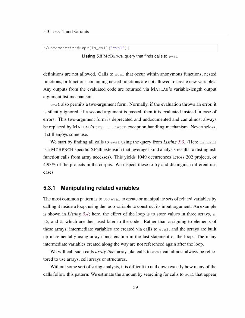
5.3. eval and variants
//ParameterizedExpr[is_call(’eval’)]
Listing 5.3 MCBENCH query that finds calls to eval
definitions are not allowed. Calls to eval that occur within anonymous functions, nested
functions, or functions containing nested functions are not allowed to create new variables.
Any outputs from the evaluated code are returned via MATLAB’s variable-length output
argument list mechanism.
eval also permits a two-argument form. Normally, if the evaluation throws an error, it
is silently ignored; if a second argument is passed, then it is evaluated instead in case of
errors. This two-argument form is deprecated and undocumented and can almost always
be replaced by MATLAB’s try ... catch exception handling mechanism. Nevertheless,
it still enjoys some use.
We start by finding all calls to eval using the query from Listing 5.3. (Here is_call
is a MCBENCH-specific XPath extension that leverages kind analysis results to distinguish
function calls from array accesses). This yields 1049 occurrences across 202 projects, or
4.93% of the projects in the corpus. We inspect these to try and distinguish different use
cases.
5.3.1 Manipulating related variables
The most common pattern is to use eval to create or manipulate sets of related variables by
calling it inside a loop, using the loop variable to construct its input argument. An example
is shown in Listing 5.4; here, the effect of the loop is to store values in three arrays, n,
s2, and Z, which are then used later in the code. Rather than assigning to elements of
these arrays, intermediate variables are created via calls to eval, and the arrays are built
up incrementally using array concatenation in the last statement of the loop. The many
intermediate variables created along the way are not referenced again after the loop.
We will call such calls array-like; array-like calls to eval can almost always be refac-
tored to use arrays, cell arrays or structures.
Without some sort of string analysis, it is difficult to nail down exactly how many of the
calls follow this pattern. We estimate the amount by searching for calls to eval that appear
59

Survey of Dynamic Features
%Levene’s Procedure.
n=[];s2=[];Z=[];
indice=Y(:,2);
for i=1:k
Ye=find(indice==i);
eval([’Y’ num2str(i) ’=Y(Ye,1);’]);
eval([’mY’ num2str(i) ’=mean(Y(Ye,1));’]);
eval([’n’ num2str(i) ’=length(Y’ num2str(i) ’) ;’]);
eval([’s2’ num2str(i) ’=(std(Y’ num2str(i) ’).^2) ;’]);
eval([’Z’ num2str(i) ’= abs((Y’ num2str(i) ’) - mY’ num2str(i) ’);’]);
eval([’xn= n’ num2str(i) ’;’]);
eval([’xs2= s2’ num2str(i) ’;’]);
eval([’x= Z’ num2str(i) ’;’]);
n=[n;xn];s2=[s2;xs2];Z=[Z;x];
end
Listing 5.4 An iterative numerical procedure implemented using repeated calls to eval instead
of arrays.
inside a for-loop, and that have as descendents either calls to num2str or int2str where
the argument is the loop variable, or calls to sprintf where the loop variable appears
somewhere. This is difficult to express in XPath, so we cheat a little by introducing an
extension function called loopvars(), which computes the set of loop variable names in
the current context by walking up the AST, finding for statements and inspecting their
header. The resulting query is given in Listing 5.5, reports 300 occurrences across 33
benchmarks, or nearly a third of all calls to eval.
This is an underestimate, since the query only matches calls where the argument string
is constructed syntactically inside the argument list; for instance, the query won’t match
calls where the string interpolation is hidden behind a function call, or if the call is of the
form eval(s) where s was previously defined according to our criteria. It may be possible
to annotate the XML form of the AST with enough semantic information (for instance, UD
chains) to enable more sophisticated queries.
5.3.2 Restricted calls to eval
As mentioned, calls to eval ocurring within anonymous functions, nested functions, or
functions containing nested functions are not allowed to create variables. Such calls turn
60
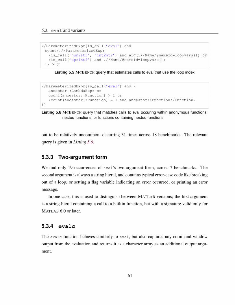
5.3. eval and variants
//ParameterizedExpr[is_call(’eval’) and
count(.//ParameterizedExpr[
(is_call(’num2str’, ’int2str’) and arg(1)/Name/@nameId=loopvars()) or
(is_call(’sprintf’) and .//Name/@nameId=loopvars())
]) > 0]
Listing 5.5 MCBENCH query that estimates calls to eval that use the loop index
//ParameterizedExpr[is_call(’eval’) and (
ancestor::LambdaExpr or
count(ancestor::Function) > 1 or
(count(ancestor::Function) = 1 and ancestor::Function//Function)
)]
Listing 5.6 MCBENCH query that matches calls to eval occuring within anonymous functions,
nested functions, or functions containing nested functions
out to be relatively uncommon, occurring 31 times across 18 benchmarks. The relevant
query is given in Listing 5.6.
5.3.3 Two-argument form
We find only 19 occurrences of eval’s two-argument form, across 7 benchmarks. The
second argument is always a string literal, and contains typical error-case code like breaking
out of a loop, or setting a flag variable indicating an error occurred, or printing an error
message.
In one case, this is used to distinguish between MATLAB versions; the first argument
is a string literal containing a call to a builtin function, but with a signature valid only for
MATLAB 6.0 or later.
5.3.4 evalc
The evalc function behaves similarly to eval, but also captures any command window
output from the evaluation and returns it as a character array as an additional output argu-
ment.
61
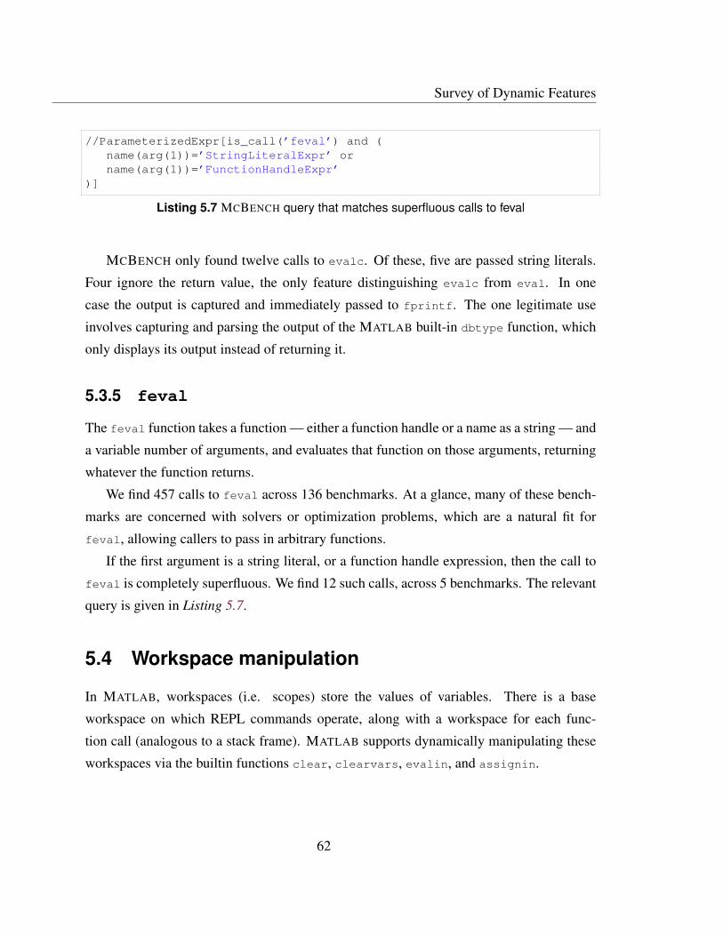
Survey of Dynamic Features
//ParameterizedExpr[is_call(’feval’) and (
name(arg(1))=’StringLiteralExpr’ or
name(arg(1))=’FunctionHandleExpr’
)]
Listing 5.7 MCBENCH query that matches superfluous calls to feval
MCBENCH only found twelve calls to evalc. Of these, five are passed string literals.
Four ignore the return value, the only feature distinguishing evalc from eval. In one
case the output is captured and immediately passed to fprintf. The one legitimate use
involves capturing and parsing the output of the MATLAB built-in dbtype function, which
only displays its output instead of returning it.
5.3.5 feval
The feval function takes a function — either a function handle or a name as a string — and
a variable number of arguments, and evaluates that function on those arguments, returning
whatever the function returns.
We find 457 calls to feval across 136 benchmarks. At a glance, many of these bench-
marks are concerned with solvers or optimization problems, which are a natural fit for
feval, allowing callers to pass in arbitrary functions.
If the first argument is a string literal, or a function handle expression, then the call to
feval is completely superfluous. We find 12 such calls, across 5 benchmarks. The relevant
query is given in Listing 5.7.
5.4 Workspace manipulation
In MATLAB, workspaces (i.e. scopes) store the values of variables. There is a base
workspace on which REPL commands operate, along with a workspace for each func-
tion call (analogous to a stack frame). MATLAB supports dynamically manipulating these
workspaces via the builtin functions clear, clearvars, evalin, and assignin.
62
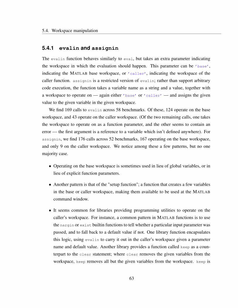
5.4. Workspace manipulation
5.4.1 evalin and assignin
The evalin function behaves similarly to eval, but takes an extra parameter indicating
the workspace in which the evaluation should happen. This parameter can be ’base’,
indicating the MATLAB base workspace, or ’caller’, indicating the workspace of the
caller function. assignin is a restricted version of evalin; rather than support arbitrary
code execution, the function takes a variable name as a string and a value, together with
a workspace to operate on — again either ’base’ or ’caller’ — and assigns the given
value to the given variable in the given workspace.
We find 169 calls to evalin across 58 benchmarks. Of these, 124 operate on the base
workspace, and 43 operate on the caller workspace. (Of the two remaining calls, one takes
the workspace to operate on as a function parameter, and the other seems to contain an
error — the first argument is a reference to a variable which isn’t defined anywhere). For
assignin, we find 176 calls across 52 benchmarks, 167 operating on the base workspace,
and only 9 on the caller workspace. We notice among these a few patterns, but no one
majority case.
• Operating on the base workspace is sometimes used in lieu of global variables, or in
lieu of explicit function parameters.
• Another pattern is that of the "setup function"; a function that creates a few variables
in the base or caller workspace, making them available to be used at the MATLAB
command window.
• It seems common for libraries providing programming utilities to operate on the
caller’s workspace. For instance, a common pattern in MATLAB functions is to use
the nargin or exist builtin functions to tell whether a particular input parameter was
passed, and to fall back to a default value if not. One library function encapsulates
this logic, using evalin to carry it out in the caller’s workspace given a parameter
name and default value. Another library provides a function called keep as a coun-
terpart to the clear statement; where clear removes the given variables from the
workspace, keep removes all but the given variables from the workspace. keep is
63
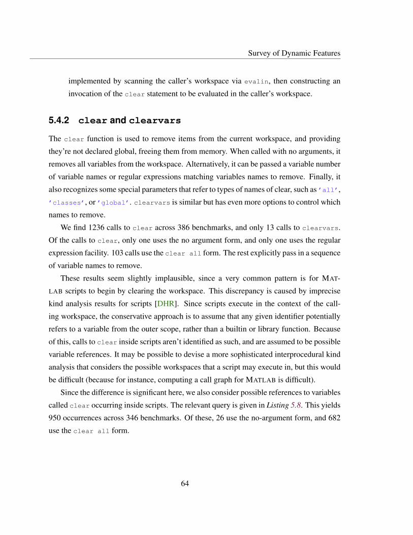
Survey of Dynamic Features
implemented by scanning the caller’s workspace via evalin, then constructing an
invocation of the clear statement to be evaluated in the caller’s workspace.
5.4.2 clear and clearvars
The clear function is used to remove items from the current workspace, and providing
they’re not declared global, freeing them from memory. When called with no arguments, it
removes all variables from the workspace. Alternatively, it can be passed a variable number
of variable names or regular expressions matching variables names to remove. Finally, it
also recognizes some special parameters that refer to types of names of clear, such as ’all’,
’classes’, or ’global’. clearvars is similar but has even more options to control which
names to remove.
We find 1236 calls to clear across 386 benchmarks, and only 13 calls to clearvars.
Of the calls to clear, only one uses the no argument form, and only one uses the regular
expression facility. 103 calls use the clear all form. The rest explicitly pass in a sequence
of variable names to remove.
These results seem slightly implausible, since a very common pattern is for MAT-
LAB scripts to begin by clearing the workspace. This discrepancy is caused by imprecise
kind analysis results for scripts [DHR]. Since scripts execute in the context of the call-
ing workspace, the conservative approach is to assume that any given identifier potentially
refers to a variable from the outer scope, rather than a builtin or library function. Because
of this, calls to clear inside scripts aren’t identified as such, and are assumed to be possible
variable references. It may be possible to devise a more sophisticated interprocedural kind
analysis that considers the possible workspaces that a script may execute in, but this would
be difficult (because for instance, computing a call graph for MATLAB is difficult).
Since the difference is significant here, we also consider possible references to variables
called clear occurring inside scripts. The relevant query is given in Listing 5.8. This yields
950 occurrences across 346 benchmarks. Of these, 26 use the no-argument form, and 682
use the clear all form.
64
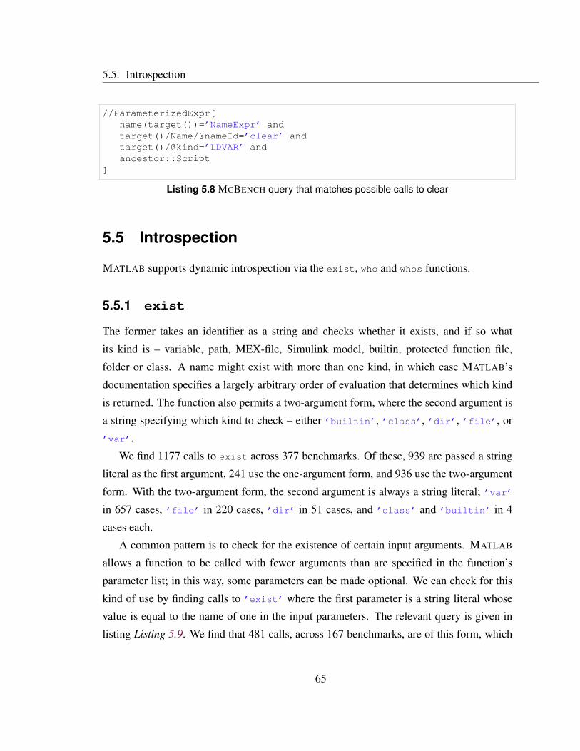
5.5. Introspection
//ParameterizedExpr[
name(target())=’NameExpr’ and
target()/Name/@nameId=’clear’ and
target()/@kind=’LDVAR’ and
ancestor::Script
]
Listing 5.8 MCBENCH query that matches possible calls to clear
5.5 Introspection
MATLAB supports dynamic introspection via the exist, who and whos functions.
5.5.1 exist
The former takes an identifier as a string and checks whether it exists, and if so what
its kind is – variable, path, MEX-file, Simulink model, builtin, protected function file,
folder or class. A name might exist with more than one kind, in which case MATLAB’s
documentation specifies a largely arbitrary order of evaluation that determines which kind
is returned. The function also permits a two-argument form, where the second argument is
a string specifying which kind to check – either ’builtin’, ’class’, ’dir’, ’file’, or
’var’.
We find 1177 calls to exist across 377 benchmarks. Of these, 939 are passed a string
literal as the first argument, 241 use the one-argument form, and 936 use the two-argument
form. With the two-argument form, the second argument is always a string literal; ’var’
in 657 cases, ’file’ in 220 cases, ’dir’ in 51 cases, and ’class’ and ’builtin’ in 4
cases each.
A common pattern is to check for the existence of certain input arguments. MATLAB
allows a function to be called with fewer arguments than are specified in the function’s
parameter list; in this way, some parameters can be made optional. We can check for this
kind of use by finding calls to ’exist’ where the first parameter is a string literal whose
value is equal to the name of one in the input parameters. The relevant query is given in
listing Listing 5.9. We find that 481 calls, across 167 benchmarks, are of this form, which
65
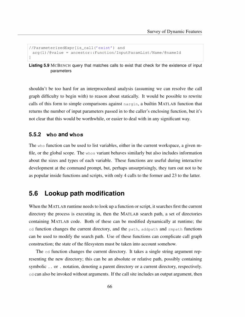
Survey of Dynamic Features
//ParameterizedExpr[is_call(’exist’) and
arg(1)/@value = ancestor::Function/InputParamList/Name/@nameId
]
Listing 5.9 MCBENCH query that matches calls to exist that check for the existence of input
parameters
shouldn’t be too hard for an interprocedural analysis (assuming we can resolve the call
graph difficulty to begin with) to reason about statically. It would be possible to rewrite
calls of this form to simple comparisons against nargin, a builtin MATLAB function that
returns the number of input parameters passed in to the caller’s enclosing function, but it’s
not clear that this would be worthwhile, or easier to deal with in any significant way.
5.5.2 who and whos
The who function can be used to list variables, either in the current workspace, a given m-
file, or the global scope. The whos variant behaves similarly but also includes information
about the sizes and types of each variable. These functions are useful during interactive
development at the command prompt, but, perhaps unsurprisingly, they turn out not to be
as popular inside functions and scripts, with only 4 calls to the former and 23 to the latter.
5.6 Lookup path modification
When the MATLAB runtime needs to look up a function or script, it searches first the current
directory the process is executing in, then the MATLAB search path, a set of directories
containing MATLAB code. Both of these can be modified dynamically at runtime; the
cd function changes the current directory, and the path, addpath and rmpath functions
can be used to modify the search path. Use of these functions can complicate call graph
construction; the state of the filesystem must be taken into account somehow.
The cd function changes the current directory. It takes a single string argument rep-
resenting the new directory; this can be an absolute or relative path, possibly containing
symbolic .. or . notation, denoting a parent directory or a current directory, respectively.
cd can also be invoked without arguments. If the call site includes an output argument, then
66

5.6. Lookup path modification
cd returns the absolute path to the present working directory as a string. If not, it writes the
path to standard output.
We find 187 calls to cd across 64 benchmarks. Most often, cd is used to get at data that
the program depends on; the working directory is changed to a data folder, and functions
such as load or textread are then used to read in the data, passing in only the file name,
without any leading directory names. In many cases, cd is called again immediately after
loading the data, so as to restore the original working directory. Rather than carrying out
this sort of dance, it would be preferable to load the required data using a path relative to
the starting working directory.
The addpath function can be used to insert directories either at the start or end of
the MATLAB search path. It takes a variable number of strings as arguments, optionally
followed by the string ’-begin’ or ’-end’, denoting whether to insert the directories at
the start or end of the path. The default behavior is to add them at the start. It returns the
old path.
The rmpath function removes a directory from the search path. It takes a single string
argument and returns nothing.
The path function is more powerful; it can be used to add paths to the start or end of the
search path, but it can also be passed a string array representing a list of folders to replace
the search path entirely. It returns the old path. This function can also be used to read the
path, without modifying it.
Finally, there also exists a restoredefaultpath function that discards any modifica-
tions to the search path, and a savepath function that persists any modifications to the
search path to be used by future MATLAB sessions.
We find 20 calls to addpath across 16 benchmarks, 4 calls to rmpath across 4 bench-
marks, 31 calls to path across 15 benchmarks – 18 of which use the two-argument form
equivalent to addpath, and 13 the one-argument form replacing the path. We find no calls
to restoredefaultpath or savepath.
67

Survey of Dynamic Features
5.7 Motivation for eliminating uses of dynamic features
While dynamic features are very powerful, for instance enabling metaprogramming tech-
niques that aren’t otherwise possible, they also have many drawbacks.
5.7.1 Impact on static analysis and program comprehension
Compilers and related tools rely on various static analyses to estimate the runtime behavior
of programs. Such analyses are typically conservative, preferring to deduce weaker prop-
erties that are guaranteed to always hold for all inputs over stronger properties that might
not always hold, even if the latter would be more useful. This ensures the soundness of any
ensuing program transformations (such as optimizations) predicated on those analyses.
Highly dynamic features tend to confuse traditional static analysis techniques. For ex-
ample, a call to eval can have nearly arbitrary side effects. Without knowing the exact
values passed as arguments – information which is rarely knowable statically – encoun-
tering a call to eval forces a conservative analysis to invalidate all the knowledge it has
gathered thus far and fall back on safe assumptions. As clients consume the analysis infor-
mation, this imprecision leads to missed optimization opportunities in compilers, crippled
code navigation features in IDEs, and spurious warnings in static analyzers, among others.
eval is an easy example to pick on, being the most general and powerful dynamic con-
struct, but other dynamic features also lead to imprecision. Changing the function lookup
path obsoletes static information gathered about the call graph. Reaching into another
function’s workspace and assigning to a variable invalidates information about identifier
lookup, making it hard to distinguish between array accesses and function calls. Loading
data via calls to the load function complicates reasoning about the shapes of arrays.
5.7.2 Performance
One of the main observations of this section is that many uses of dynamic features are
completely superfluous, and could be equivalently written using simpler, less powerful
constructs of the language. In those cases, it makes sense to consider the performance
characteristics of the two approaches.
68
5.8. Related work
As an example, one of the principal patterns identified concerns using repeated calls
to the eval family of functions in a loop in lieu of using arrays. The code in Listing 5.4
calls eval, invoking the full machinery of the interpreter, no fewer than eight times per loop
iteration, even though each of these could be replaced by two or three array operations. This
has a huge impact on performance. As a preliminary test, we manually replaced each call
to eval in that benchmark with equivalent code using arrays. The transformed benchmark
achieved a 56x speedup over the original.
Beyond interpreter overhead, code that restricts itself to features that are easier to rea-
son about statically is apt to be better understood by compilers, which rely on sophisti-
cated static analysis to identify candidates for optimization. This is not irrelevant; several
MATLAB compilers exist, and recent versions of the proprietary MATLAB implementation
include a JIT compiler.
5.8 Related work
5.8.1 Dynamic feature survey
This study is inspired in part by Furr et al.’s work on profile-guided static typing for Ruby
[FhDAF09], where one of the major insights was that although highly dynamic semantics
can theoretically lead to code which is hard to reason about, dynamic features tend to be
used is much more restricted ways in practice. Similar studies done for JavaScript by
Ratanaworabhan et al. [RLZ10] and Richards et al. [RHBV11, RLBV10] have reached
similar conclusions. Because JavaScript is so ubiquitous on the web, one can instrument
a web browser and visit popular web pages to obtain all sorts of dynamic metrics. The
same is unfortunately not true in our case; although we have easy access to a large body of
MATLAB code, it is not trivial in general to determine how to execute it, which is why we
had to restrict ourselves to static metrics.
69

Survey of Dynamic Features
5.8.2 Dynamic feature elimination
Furr et al. [FhDAF09] present a dynamic profiling approach to eliminate uses of Ruby’s
dynamic features like eval, send and method_missing, with the aim is making code more
amenable to static analysis. They use a profiling run to gather information at each dynamic
use site, for instance the actual arguments passed to eval, or the actual missing methods
for which method_missing was invoked, and use this to replace the usage sites with spe-
cialized code for each observed argument (along with runtime checks to emit warnings in
case the arguments used don’t conform to the profiling run).
In the wake of the abovementioned studies conducted by Richards et al. [RLBV10,
RHBV11], there has been some work on eliminating uses of eval in JavaScript. The
common thread is exploiting patterns in the way eval tends to be used, be it for parsing
JSON strings, executing third party code, or accessing or modifying object properties with
computed names.
Jensen et al.’s Unevalizer tool [JJM12] integrates a refactoring component with a static
whole-program value dataflow analysis. When the analysis detects dataflow into a possible
call to eval, it triggers the refactoring component, passing in all the information it has
gathered so far about the values of variables. Guided by knowledge of common patterns,
the refactoring component attempts to replace the code with a static equivalent if possible.
If so, the analysis resumes until all calls to eval are eliminated; if not, the tool aborts with
an error. Their approach enjoys moderate success, but is hindered by the imprecision of
their static analysis in various cases.
Meawad et al.’s [MRMV12] Evalorizer tool instruments all calls to eval, intercepting
and logging all the strings passed at each call site. For each particular call site, each ar-
gument string is taken to be valid JavaScript and parsed into an AST. The different ASTs
are then merged together and generalized in different ways in order to construct a "recog-
nizer" tree associated with that call site, which is then used to generate patches containing
replacement code. The replacement code contains a runtime guard clause checking that the
passed in argument matches the pattern observed for this call site – this can be done with a
regular expression in most cases. If it does, then safer but equivalent code is run; if not, a
fallback case contains the original call to eval (or optionally an exception, if the tool is so
70

5.8. Related work
configured). This approach turns out to be fruitful, and the patched code runs with minimal
performance overhead.
71

Survey of Dynamic Features
72
Chapter 6
Conclusions and Future Work
This thesis introduced McIDE, a MATLAB IDE powered by the McLAB compiler
toolkit, and with a focus on powering features through exploiting runtime information
rather than relying solely on static analysis. We provided an overview of McIDE’s design,
which consists of largely independent components wired together through a thin browser-
based graphical interface. We described our dynamic call graph collection mechanism, and
the analyses and optimizations we implemented to minimize the performance overhead of
the instrumented code. We presented a technique for performing code transformations in a
layout-preserving fashion, which allows McIDE to provide some usable automated refac-
torings out of the box, and future refactoring implementers to reuse the transformation
infrastructure to do the same. Finally, we described MATLAB’s dynamic features in detail
and presented a study of their usage in the wild.
6.1 Future Work
We present here some ideas for possible further work for the continued development of
McIDE. The common thread is finding more useful ways to exploit runtime information.
Dynamic feature elimination The dynamic feature survey we conducted pointed to a few
patterns where dynamic code could easily be rewritten using more static analysis
friendly constructs. It may be hard to do this in general, but one could tackle the
73
Conclusions and Future Work
problem of replacing the array-like uses of eval with straightforward loops, or elim-
inating uses of cd where the aim is only to refer to data to be loaded from the filesys-
tem.
Making code more ameanable to static analysis would also make it more suitable
as input to static backends of the McLAB toolkit, which operate on the MATLAB
subset supported by the MATLAB Tamer, which rules out features like eval. If static
compilation is a goal for the user, then more work is this vein could help compatibility
along.
Dynamic code visualizations IDEs are in a position to provide alternate perspectives on
the code beyond the traditional file explorer view, and runtime information could be
particularly useful in this setting.
As low hanging fruit, the call graph information described in this thesis could be used
to show execution stack traces as a tree and enable jumping directly to any function
invoked along the way.
Relevant runtime information could be overlaid onto source code in order to aid pro-
gram understanding – expressions could be annotated with runtime types (or even
values), perhaps via tooltips or comments introduced into the code if requested; lines
of code could be annotated with timing information, for instance by coloring bot-
tlenecks differently as to make them stand out; the profiling machinery could work
backwards from errors in the execution to highlight the problematic code paths.
74

Bibliography
[AL12] Karim Ali and Ondrej Lhoták. Application-only call graph construction. In
Proceedings of the 26th European Conference on Object-Oriented Program-
ming, Beijing, China, 2012, ECOOP’12, pages 688–712. Springer-Verlag,
Berlin, Heidelberg.
[CLD+10] Andrew Casey, Jun Li, Jesse Doherty, Maxime Chevalier-Boisvert, To-
heed Aslam, Anton Dubrau, Nurudeen Lameed, Amina Aslam, Rahul Garg,
Soroush Radpour, Olivier Savary Belanger, Laurie Hendren, and Clark Ver-
brugge. Mclab: an extensible compiler toolkit for matlab and related lan-
guages. In Proceedings of the Third C* Conference on Computer Science
and Software Engineering, Montrà c©al, Quebec, Canada, 2010, C3S2E ’10,
pages 114–117. ACM, New York, NY, USA.
[DGL06] Marcus Denker, Orla Greevy, and Michele Lanza. Higher abstractions for dy-
namic analysis. In In 2nd International Workshop on Program Comprehension
through Dynamic Analysis (PCODA 2006), 2006, pages 32–38.
[DH12] Anton Willy Dubrau and Laurie Jane Hendren. Taming MATLAB. In
Proceedings of the ACM international conference on Object oriented pro-
gramming systems languages and applications, Tucson, Arizona, USA, 2012,
OOPSLA ’12, pages 503–522. ACM, New York, NY, USA.
75
Bibliography
[DHR] Jesse Doherty, Laurie Hendren, and Soroush Radpour. Kind analysis for MAT-
LAB. In Proceedings of the 2011 ACM International Conference on Object
Oriented Programming Systems Languages and Applications, OOPSLA ’11,
pages 99–118. ACM.
[dJV12] Maartje de Jonge and Eelco Visser. An algorithm for layout preservation in
refactoring transformations. In Anthony Sloane and Uwe Aßmann, editors,
Software Language Engineering, volume 6940 of Lecture Notes in Computer
Science, pages 40–59. Springer Berlin Heidelberg, 2012.
[FhDAF09] Michael Furr, Jong hoon (David) An, and Jeffrey S. Foster. Profile-guided
static typing for dynamic scripting languages. In OOPSLA, 2009, pages 283–
300.
[FSS+13] Asger Feldthaus, Max Schäfer, Manu Sridharan, Julian Dolby, and Frank Tip.
Efficient construction of approximate call graphs for JavaScript IDE services.
In Proceedings of the 2013 International Conference on Software Engineer-
ing, San Francisco, CA, USA, 2013, ICSE ’13, pages 752–761. IEEE Press,
Piscataway, NJ, USA.
[JJM12] Simon Holm Jensen, Peter A. Jonsson, and Anders Møller. Remedying the
eval that men do. In Proc. 21st International Symposium on Software Testing
and Analysis (ISSTA), July 2012.
[KLN+09] Róbert Kitlei, László Lövei, Tamás Nagy, Zoltán Horváth, and Tamás Kozsik.
Layout preserving parser for refactoring in Erlang. Acta Electrotechnica et
Informatica, 9(3):54–63, July 2009.
[LH13] Nurudeen A. Lameed and Laurie J. Hendren. Optimizing MATLAB feval
with dynamic techniques. In Proceedings of the 9th Symposium on Dynamic
Languages, Indianapolis, Indiana, USA, 2013, DLS ’13, pages 85–96. ACM,
New York, NY, USA.
[Li06] Huiqing Li. Refactoring Haskell Programs. PhD thesis, University of Kent,
2006.
76

Bibliography
[MRMV12] Fadi Meawad, Gregor Richards, Floréal Morandat, and Jan Vitek. Eval be-
gone!: Semi-automated removal of eval from JavaScript programs. In Pro-
ceedings of the ACM International Conference on Object Oriented Program-
ming Systems Languages and Applications, Tucson, Arizona, USA, 2012,
OOPSLA ’12, pages 607–620. ACM, New York, NY, USA.
[Rad12] Soroush Radpour. Understanding and refactoring the MATLAB language.
Master’s thesis, August 2012.
[RHBV11] Gregor Richards, Christian Hammer, Brian Burg, and Jan Vitek. The eval that
men do: A large-scale study of the use of eval in JavaScript applications.
In Preceedings of the 25th European Conference on Object-oriented Pro-
gramming, Lancaster, UK, 2011, ECOOP’11, pages 52–78. Springer-Verlag,
Berlin, Heidelberg.
[RLBV10] Gregor Richards, Sylvain Lebresne, Brian Burg, and Jan Vitek. An analy-
sis of the dynamic behavior of JavaScript programs. In Proceedings of the
2010 ACM SIGPLAN Conference on Programming Language Design and Im-
plementation, Toronto, Ontario, Canada, 2010, PLDI ’10, pages 1–12. ACM,
New York, NY, USA.
[RLZ10] Paruj Ratanaworabhan, Benjamin Livshits, and Benjamin G. Zorn. JSMeter:
Comparing the behavior of JavaScript benchmarks with real web applications.
In Proceedings of the 2010 USENIX Conference on Web Application Devel-
opment, Boston, MA, 2010, WebApps’10, pages 3–3. USENIX Association,
Berkeley, CA, USA.
[WR13] Shiyi Wei and Barbara G. Ryder. Practical blended taint analysis for
JavaScript. In Proceedings of the 2013 International Symposium on Soft-
ware Testing and Analysis, Lugano, Switzerland, 2013, ISSTA 2013, pages
336–346. ACM, New York, NY, USA.
[WY05] Daniel G Waddington and Bin Yao. High-fidelity C/C++ code transformation.
Electronic Notes in Theoretical Computer Science, 141(4):35–36, 2005.
77