HAL Id: hal-00806835https://hal.archives-ouvertes.fr/hal-00806835

Submitted on 2 Apr 2013

HAL is a multi-disciplinary open accessarchive for the deposit and dissemination of sci-entific research documents, whether they are pub-lished or not. The documents may come fromteaching and research institutions in France orabroad, or from public or private research centers.

L’archive ouverte pluridisciplinaire HAL, estdestinée au dépôt et à la diffusion de documentsscientifiques de niveau recherche, publiés ou non,émanant des établissements d’enseignement et derecherche français ou étrangers, des laboratoirespublics ou privés.

MCALab: Reproducible Research in Signal and ImageDecomposition and Inpainting

Jalal M. Fadili, Jean-Luc Starck, Michael Elad, David Donoho

To cite this version:Jalal M. Fadili, Jean-Luc Starck, Michael Elad, David Donoho. MCALab: Reproducible Research inSignal and Image Decomposition and Inpainting. IEEE Computing in Science and Engineering, 2010,12 (1), pp.44 - 63. <10.1109/MCSE.2010.14>. <hal-00806835>

1

MCALab: Reproducible Research in Signal and

Image Decomposition and Inpainting

M.J. Fadili , J.-L. Starck , M. Elad and D.L. Donoho

Abstract

Morphological Component Analysis (MCA) of signals and images is an ambitious and important goal

in signal processing; successful methods for MCA have many far-reaching applications in science and tech-

nology. Because MCA is related to solving underdetermined systems of linear equations it might also be

considered, by some, to be problematic or even intractable. Reproducible research is essential to to give such

a concept a firm scientific foundation and broad base of trusted results.

MCALab has been developed to demonstrate key concepts of MCA and make them available to interested

researchers and technologists. MCALab is a library of Matlab routines that implement the decomposition and

inpainting algorithms that we previously proposed in [1], [2], [3], [4]. The MCALab package provides the

research community with open source tools for sparse decomposition and inpainting and is made available

for anonymous download over the Internet. It contains a variety of scripts to reproduce the figures in our

own articles, as well as other exploratory examples not included in the papers. One can also run the same

experiments on one’s own data or tune the parameters by simply modifying the scripts. The MCALab is under

continuing development by the authors; who welcome feedback and suggestions for further enhancements,

and any contributions by interested researchers.

Index Terms

Reproducible research, sparse representations, signal and image decomposition, inpainting, Morphologi-

cal Component Analysis.

M.J. Fadili is with the CNRS-ENSICAEN-Universite de Caen, Image Processing Group, ENSICAEN 14050, Caen Cedex, France.

J.-L. Starck is with the LAIM, CEA/DSM-CNRS-Universite Paris Diderot, IRFU, SEDI-SAP, 91191 Gif-Sur-Yvette cedex, France.

M. Elad is with the Department of Computer Science, Technion, 32000 Haifa, Israel.

D.L. Donoho is with the Department of Statistics, Sequoia Hall, Stanford, CA, USA.

June 19, 2009 DRAFT

2

I. INTRODUCTION

A. Reproducible research

Reproducibility is at the heart of scientific methodology and all successful technology development. In

theoretical disciplines, the gold standard has been set by mathematics, where formal proof in principle allows

anyone to reproduce the cognitive steps leading to verification of a theorem. In experimental disciplines, such

as biology, physics or chemistry, for a result to be well-established, particular attention is paid to experiment

replication. Of course, a necessary condition to truthfully replicate the experiment is that the paper has to

describe it with enough detail to allow another group to mimic it.

Computational science is a much younger field than mathematics, but already of great importance for human

welfare; however reproducibility has not yet become a rigorously-adhered to notion. The slogan ’reproducible

research’ is of relatively recent coinage, and tries to create a real gold standard for computational reproducibil-

ity; it recognizes that the real outcome of a research project is not the published article, but rather the entire

environment used to reproduce the results presented in the paper, including data, software, documentation, etc

[5]. A closely-related concept to reproducible research is computational provenance. In scientific experiments,

provenance helps interpret and understand results by examining the sequence of steps that led to a result. In a

sense, potential uses of provenance go beyond reproducibility; see May/June 2008 CiSE issue on this subject

[6].

Inspired by Clearbout, Donoho in the early 1990’s began to practice reproducible research in computational

harmonic analysis within the now-proliferating quantitative programming environment Matlab; see the review

paper [7] in the January/February 2009 CiSE special issue on reproducible research. In the signal processing

community, the interest in reproducible research was revitalized in [8]. At one of the major signal processing

conferences, ICASSP 2007, a special session was entirely devoted to reproducible signal processing research.

B. This paper

In this paper, reproducible research is discussed in the context of sparse-representation-based signal/image

decomposition and inpainting. We introduce MCALab, a library of Matlab routines that implements the

algorithms proposed by the authors in [2], [3], [4] for signal/image decomposition and inpainting. The library

provides the research community with open source tools for sparse decomposition and inpainting, and may be

used to reproduce the figures in this paper and to redo those figures with variations in the parameters.

Although Mathematics has it million-dollar problems, in the form of Clay Math Prizes, there are several

Billion Dollar problems in signal and image processing. Famous ones include the phase problem (loss of

information from a physical measurement) and the cocktail party problem (separate one sound from a mixture

of other recorded sounds and background noises at a cocktail party). The “Billion Dollar” adjective refers to

June 19, 2009 DRAFT

3

the enormous significance of these problems in the world economy if these problems were solved, as well as

the extreme intellectual ‘kick’ a solution would necessarily entail. These signal processing problems seem to

be intractable according to orthodox arguments based on rigorous mathematics, and yet they keep cropping up

in problem after problem.

One such fundamental problem involves decomposing a signal or image into superposed contributions from

different sources; think of symphonic music which may involve superpositions of acoustic signals generated by

many different instruments – and imagine the problem of separating these contributions. More abstractly, we

can see many forms of media content that are superpositions of contributions from different ‘content types’,

and we can imagine wanting to separate out the contributions from each. We can easily see a fundamental

problem; for example an n-pixel image created by superposing K different types offers us n data (the pixel

values) but there may be as many as n · K unknowns (the contribution of each content type to each pixel).

Traditional mathematical reasoning, in fact the fundamental theorem of linear algebra, tells us not to attempt

this: there are more unknowns than equations. On the other hand, if we have prior information about the

underlying object, there are some rigorous results showing that such separation might be possible – using

special techniques. We are left with the situation of grounds for both hope and skepticism.

The idea to morphologically decompose a signal into its building blocks is an important problem in signal

and image processing. An interesting and complicated image content separation problem is the one targeting

decomposition of an image to texture and piece-wise-smooth (cartoon) parts. Since the pioneering contribution

of the French mathematician Yves Meyer [9], we have witnessed a flurry of research activity in this application

field. Successful methods for signal or image separation can be applied in a broad range of areas in science

and technology including biomedical engineering, medical imaging, speech processing, astronomical imaging,

remote sensing, communication systems, etc.

In [1], [2] a novel decomposition method – Morphological Component Analysis (MCA) – based on sparse

representation of signals. MCA assumes that each signal is the linear mixture of several layers, the so-

called Morphological Components, that are morphologically distinct, e.g. sines and bumps. The success of

this method relies on the assumption that for every signal atomic behavior to be separated, there exists a

dictionary of atoms that enables its construction using a sparse representation. It is then assumed that each

morphological component is sparsely represented in a specific transform domain. And when all transforms

(each one attached to a morphological component) are amalgamated in one dictionary, each one must lead

to sparse representation over the part of the signal it is serving, while being highly inefficient in representing

the other content in the mixture. If such dictionaries are identified, the use of a pursuit algorithm searching

for the sparsest representation leads to the desired separation. MCA is capable of creating atomic sparse

representations containing as a by-product a decoupling of the signal content. In [3], MCA has been extended

to simultaneous texture and cartoon images inpainting. In [4], the authors formalized the inpainting problem

June 19, 2009 DRAFT

4

as a missing data estimation problem.

II. THEORY AND ALGORITHMS

Before describing of the MCALab library, let’s first explain the terminology used throughout the paper,

review the main theoretical concepts and give the gist of the algorithms.

A. Terminology

Atom: An atom is an elementary signal-representing template. Examples might include sinusoids, mono-

mials, wavelets, Gaussians. Using a collection of atoms as building blocks, one can construct more complex

waveforms by linear superposition.

Dictionary: A dictionary Φ is an indexed collection of atoms (φγ)γ∈Γ, where Γ is a countable set.

The interpretation of the index γ depends on the dictionary; frequency for the Fourier dictionary (i.e. sinu-

soids), position for the Dirac dictionary (aka standard unit vector basis, or kronecker basis), position-scale

for the wavelet dictionary, translation-duration-frequency for cosine packets, position-scale-orientation for the

curvelet dictionary in two dimensions. In discrete-time finite-length signal processing, a dictionary can be

viewed as a matrix whose columns are the atoms, and the atoms are considered as column vectors. When the

dictionary has more columns than rows, it is called overcomplete or redundant. We are mainly interested here

in overcomplete dictionaries. The overcomplete case is the setting where the signal x = Φα amounts to an

underdetermined system of linear equations.

Analysis and synthesis: Given a dictionary, one has to distinguish between analysis and synthesis op-

erations. Analysis is the operation which associates to each signal x a vector of coefficients α attached to

atom: α = ΦT x. Synthesis is the operation of reconstructing x by superposing atoms: x = Φα. Analysis

and synthesis are very different linear operations. In the overcomplete case, Φ is not invertible and the

reconstruction is not unique; see also subsection II-B for further details.

Morphological component: For a given n-sample signal or image x, we assume that it consists of a

sum of K signals or images (xk)k=1,··· ,K , x =∑K

k=1 xk, having different morphologies. Each xk is called a

morphological component.

Inpainting: Inpainting is to restore missing image information based upon the still available (observed)

cues from destroyed, occluded or deliberately masked subregions of the signal or image. Roughly speaking,

inpainting is an interpolation of missing or occluded data.

B. Fast implicit transforms and dictionaries

Owing to recent advances in modern harmonic analysis, many novel representations, including the wavelet

transform, curvelet, contourlet, steerable or complex wavelet pyramids, were shown to be very effective in

June 19, 2009 DRAFT

5

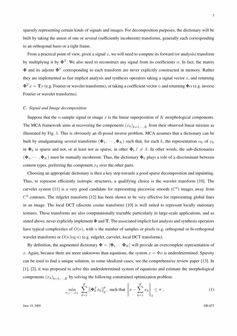
sparsely representing certain kinds of signals and images. For decomposition purposes, the dictionary will be

built by taking the union of one or several (sufficiently incoherent) transforms, generally each corresponding

to an orthogonal basis or a tight frame.

From a practical point of view, given a signal x, we will need to compute its forward (or analysis) transform

by multiplying it by ΦT . We also need to reconstruct any signal from its coefficients α. In fact, the matrix

Φ and its adjoint ΦT corresponding to each transform are never explicitly constructed in memory. Rather

they are implemented as fast implicit analysis and synthesis operators taking a signal vector x, and returning

ΦT x = Tx (e.g. Fourier or wavelet transforms), or taking a coefficient vector α and returning Φα (e.g. inverse

Fourier or wavelet transforms).

C. Signal and Image decomposition

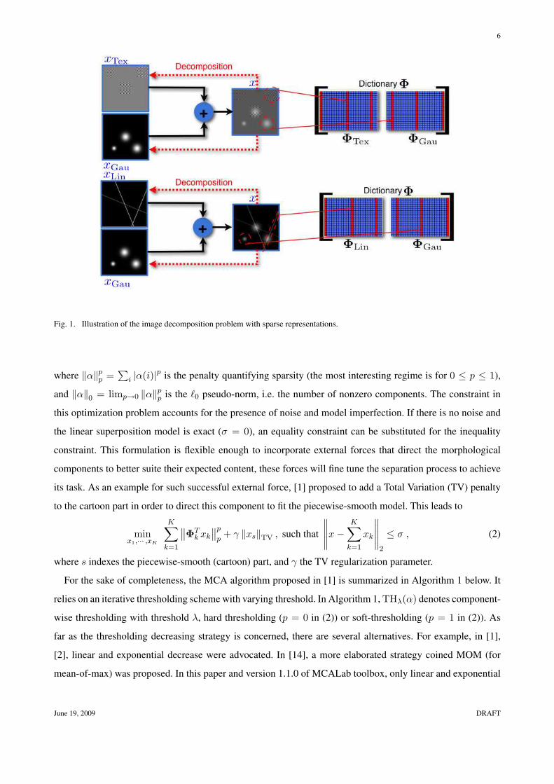
Suppose that the n-sample signal or image x is the linear superposition of K morphological components.

The MCA framework aims at recovering the components (xk)k=1,··· ,K from their observed linear mixture as

illustrated by Fig. 1. This is obviously an ill-posed inverse problem. MCA assumes that a dictionary can be

built by amalgamating several transforms (Φ1, · · · ,ΦK) such that, for each k, the representation αk of xk

in Φk is sparse and not, or at least not as sparse, in other Φl, l 6= k. In other words, the sub-dictionaries

(Φ1, · · · ,ΦK) must be mutually incoherent. Thus, the dictionary Φk plays a role of a discriminant between

content types, preferring the component xk over the other parts.

Choosing an appropriate dictionary is then a key step towards a good sparse decomposition and inpainting.

Thus, to represent efficiently isotropic structures, a qualifying choice is the wavelet transform [10]. The

curvelet system [11] is a very good candidate for representing piecewise smooth (C2) images away from

C2 contours. The ridgelet transform [12] has been shown to be very effective for representing global lines

in an image. The local DCT (discrete cosine transform) [10] is well suited to represent locally stationary

textures. These transforms are also computationally tractable particularly in large-scale applications, and as

stated above, never explicitly implement Φ and T. The associated implicit fast analysis and synthesis operators

have typical complexities of O(n), with n the number of samples or pixels (e.g. orthogonal or bi-orthogonal

wavelet transform) or O(n log n) (e.g. ridgelet, curvelet, local DCT transforms).

By definition, the augmented dictionary Φ = [Φ1 · · ·ΦK ] will provide an overcomplete representation of

x. Again, because there are more unknowns than equations, the system x = Φα is underdetermined. Sparsity

can be used to find a unique solution, in some idealized cases; see the comprehensive review paper [13]. In

[1], [2], it was proposed to solve this underdetermined system of equations and estimate the morphological

components (xk)k=1,··· ,K by solving the following constrained optimization problem:

minx1,··· ,xK

K∑

k=1

∥

∥ΦTk xk

∥

∥

p

p, such that

∥

∥

∥

∥

∥

x −K

∑

k=1

xk

∥

∥

∥

∥

∥

2

≤ σ , (1)

June 19, 2009 DRAFT

6

Fig. 1. Illustration of the image decomposition problem with sparse representations.

where ‖α‖pp =

∑

i |α(i)|p is the penalty quantifying sparsity (the most interesting regime is for 0 ≤ p ≤ 1),

and ‖α‖0 = limp→0 ‖α‖pp is the ℓ0 pseudo-norm, i.e. the number of nonzero components. The constraint in

this optimization problem accounts for the presence of noise and model imperfection. If there is no noise and

the linear superposition model is exact (σ = 0), an equality constraint can be substituted for the inequality

constraint. This formulation is flexible enough to incorporate external forces that direct the morphological

components to better suite their expected content, these forces will fine tune the separation process to achieve

its task. As an example for such successful external force, [1] proposed to add a Total Variation (TV) penalty

to the cartoon part in order to direct this component to fit the piecewise-smooth model. This leads to

minx1,··· ,xK

K∑

k=1

∥

∥ΦTk xk

∥

∥

p

p+ γ ‖xs‖TV , such that

∥

∥

∥

∥

∥

x −K

∑

k=1

xk

∥

∥

∥

∥

∥

2

≤ σ , (2)

where s indexes the piecewise-smooth (cartoon) part, and γ the TV regularization parameter.

For the sake of completeness, the MCA algorithm proposed in [1] is summarized in Algorithm 1 below. It

relies on an iterative thresholding scheme with varying threshold. In Algorithm 1, THλ(α) denotes component-

wise thresholding with threshold λ, hard thresholding (p = 0 in (2)) or soft-thresholding (p = 1 in (2)). As

far as the thresholding decreasing strategy is concerned, there are several alternatives. For example, in [1],

[2], linear and exponential decrease were advocated. In [14], a more elaborated strategy coined MOM (for

mean-of-max) was proposed. In this paper and version 1.1.0 of MCALab toolbox, only linear and exponential

June 19, 2009 DRAFT

7

decrease are implemented.

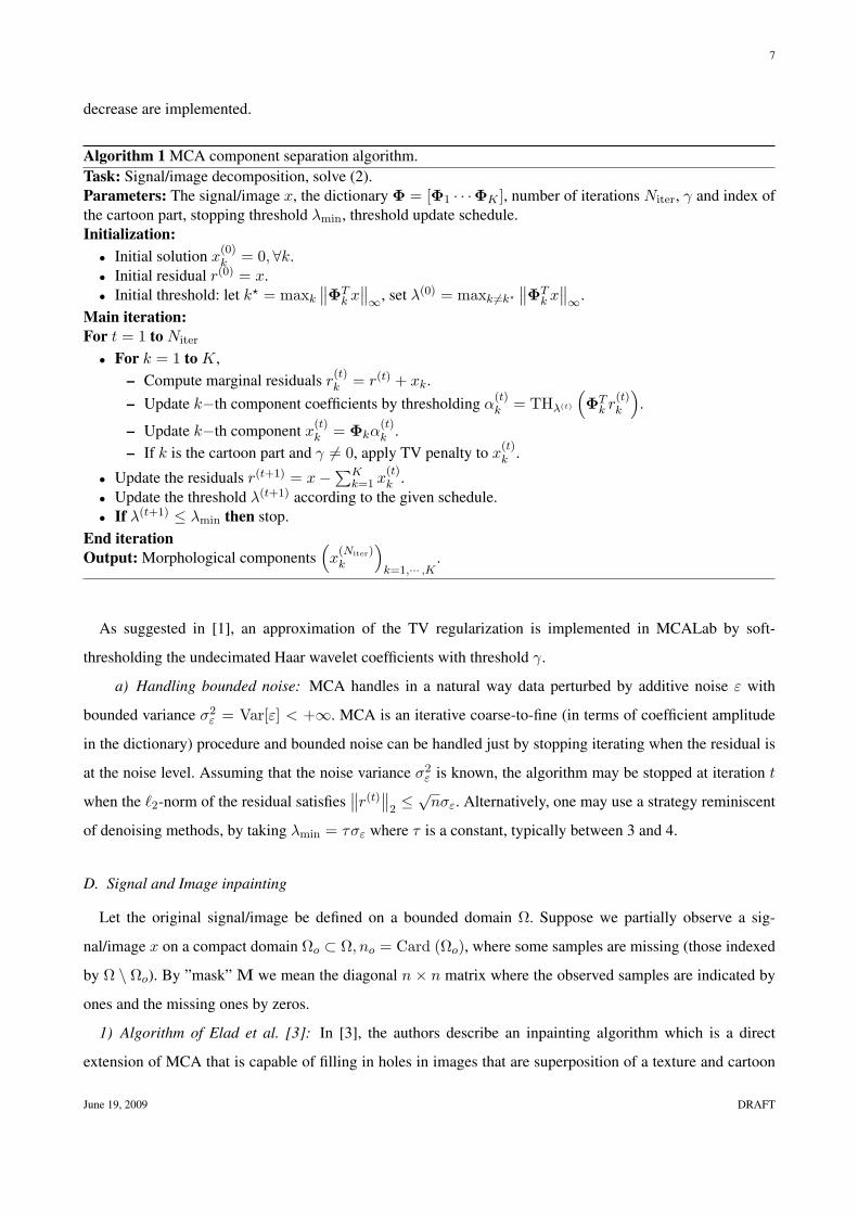
Algorithm 1 MCA component separation algorithm.

Task: Signal/image decomposition, solve (2).

Parameters: The signal/image x, the dictionary Φ = [Φ1 · · ·ΦK ], number of iterations Niter, γ and index of

the cartoon part, stopping threshold λmin, threshold update schedule.

Initialization:

• Initial solution x(0)k = 0,∀k.

• Initial residual r(0) = x.

• Initial threshold: let k⋆ = maxk

∥

∥ΦTk x

∥

∥

∞, set λ(0) = maxk 6=k⋆

∥

∥ΦTk x

∥

∥

∞.

Main iteration:

For t = 1 to Niter

• For k = 1 to K,

– Compute marginal residuals r(t)k = r(t) + xk.

– Update k−th component coefficients by thresholding α(t)k = THλ(t)

(

ΦTk r

(t)k

)

.

– Update k−th component x(t)k = Φkα

(t)k .

– If k is the cartoon part and γ 6= 0, apply TV penalty to x(t)k .

• Update the residuals r(t+1) = x − ∑Kk=1 x

(t)k .

• Update the threshold λ(t+1) according to the given schedule.

• If λ(t+1) ≤ λmin then stop.

End iteration

Output: Morphological components(

x(Niter)k

)

k=1,··· ,K.

As suggested in [1], an approximation of the TV regularization is implemented in MCALab by soft-

thresholding the undecimated Haar wavelet coefficients with threshold γ.

a) Handling bounded noise: MCA handles in a natural way data perturbed by additive noise ε with

bounded variance σ2ε = Var[ε] < +∞. MCA is an iterative coarse-to-fine (in terms of coefficient amplitude

in the dictionary) procedure and bounded noise can be handled just by stopping iterating when the residual is

at the noise level. Assuming that the noise variance σ2ε is known, the algorithm may be stopped at iteration t

when the ℓ2-norm of the residual satisfies∥

∥r(t)∥

∥

2≤ √

nσε. Alternatively, one may use a strategy reminiscent

of denoising methods, by taking λmin = τσε where τ is a constant, typically between 3 and 4.

D. Signal and Image inpainting

Let the original signal/image be defined on a bounded domain Ω. Suppose we partially observe a sig-

nal/image x on a compact domain Ωo ⊂ Ω, no = Card (Ωo), where some samples are missing (those indexed

by Ω \ Ωo). By ”mask” M we mean the diagonal n × n matrix where the observed samples are indicated by

ones and the missing ones by zeros.

1) Algorithm of Elad et al. [3]: In [3], the authors describe an inpainting algorithm which is a direct

extension of MCA that is capable of filling in holes in images that are superposition of a texture and cartoon

June 19, 2009 DRAFT

8

layers. Thus, (2) can be extended to incorporate missing data through the mask M by minimizing

minx1,··· ,xK

K∑

k=1

∥

∥ΦTk xk

∥

∥

p

p+ γ ‖xs‖TV , such that

∥

∥

∥

∥

∥

x − M

K∑

k=1

xk

∥

∥

∥

∥

∥

2

≤ σ . (3)

In our approach to solving this optimization problem, we only need to adapt slightly the MCA Algorithm 1,

modifying the residual update rule to r(t+1) = x − M∑K

k=1 x(t)k to account for the masking matrix M. The

other steps of the algorithm remain unchanged. See [3] for more details.

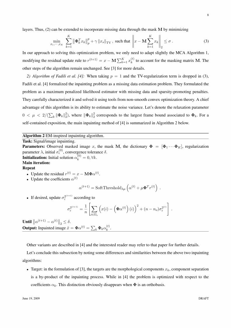
2) Algorithm of Fadili et al. [4]: When taking p = 1 and the TV-regularization term is dropped in (3),

Fadili et al. [4] formalized the inpainting problem as a missing data estimation problem. They formulated the

problem as a maximum penalized likelihood estimator with missing data and sparsity-promoting penalties.

They carefully characterized it and solved it using tools from non-smooth convex optimization theory. A chief

advantage of this algorithm is its ability to estimate the noise variance. Let’s denote the relaxation parameter

0 < µ < 2/(∑

k ‖Φk‖22), where ‖Φk‖2

2 corresponds to the largest frame bound associated to Φk. For a

self-contained exposition, the main inpainting method of [4] is summarized in Algorithm 2 below.

Algorithm 2 EM-inspired inpainting algorithm.

Task: Signal/image inpainting.

Parameters: Observed masked image x, the mask M, the dictionary Φ = [Φ1 · · ·ΦK ], regularization

parameter λ, initial σ(0)ǫ , convergence tolerance δ.

Initialization: Initial solution α(0)k = 0,∀k.

Main iteration:

Repeat

• Update the residual r(t) = x − MΦα(t).

• Update the coefficients α(t)

α(t+1) = SoftThresholdλµ

(

α(t) + µΦT r(t)

)

.

• If desired, update σ2(t+1)

ε according to

σ2(t+1)

ε =1

n

[

∑

i∈Ωo

(

x(i) −(

Φα(t))

(i))2

+ (n − no)σ2(t)

ε

]

.

Until∥

∥α(t+1) − α(t)∥

∥

2≤ δ.

Output: Inpainted image x = Φα(t) =∑

k Φkα(t)k .

Other variants are described in [4] and the interested reader may refer to that paper for further details.

Let’s conclude this subsection by noting some differences and similarities between the above two inpainting

algorithms:

• Target: in the formulation of [3], the targets are the morphological components xk, component separation

is a by-product of the inpainting process. While in [4] the problem is optimized with respect to the

coefficients αk. This distinction obviously disappears when Φ is an orthobasis.

June 19, 2009 DRAFT

9

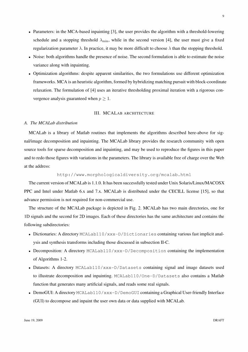
• Parameters: in the MCA-based inpainting [3], the user provides the algorithm with a threshold-lowering

schedule and a stopping threshold λmin, while in the second version [4], the user must give a fixed

regularization parameter λ. In practice, it may be more difficult to choose λ than the stopping threshold.

• Noise: both algorithms handle the presence of noise. The second formulation is able to estimate the noise

variance along with inpainting.

• Optimization algorithms: despite apparent similarities, the two formulations use different optimization

frameworks. MCA is an heuristic algorithm, formed by hybridizing matching pursuit with block-coordinate

relaxation. The formulation of [4] uses an iterative thresholding proximal iteration with a rigorous con-

vergence analysis guaranteed when p ≥ 1.

III. MCALAB ARCHITECTURE

A. The MCALab distribution

MCALab is a library of Matlab routines that implements the algorithms described here-above for sig-

nal/image decomposition and inpainting. The MCALab library provides the research community with open

source tools for sparse decomposition and inpainting, and may be used to reproduce the figures in this paper

and to redo those figures with variations in the parameters. The library is available free of charge over the Web

at the address:

http://www.morphologicaldiversity.org/mcalab.html

The current version of MCALab is 1.1.0. It has been successfully tested under Unix Solaris/Linux/MACOSX

PPC and Intel under Matlab 6.x and 7.x. MCALab is distributed under the CECILL license [15], so that

advance permission is not required for non-commercial use.

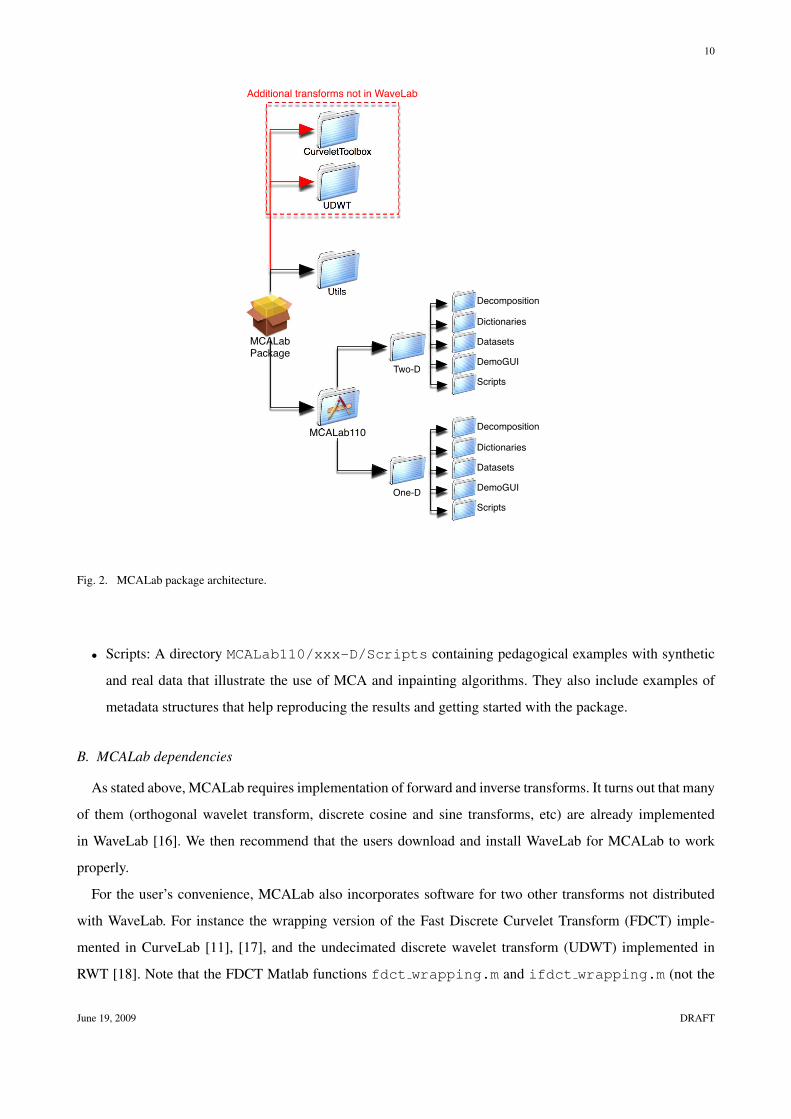
The structure of the MCALab package is depicted in Fig. 2. MCALab has two main directories, one for

1D signals and the second for 2D images. Each of these directories has the same architecture and contains the

following subdirectories:

• Dictionaries: A directory MCALab110/xxx-D/Dictionaries containing various fast implicit anal-

ysis and synthesis transforms including those discussed in subsection II-C.

• Decomposition: A directory MCALab110/xxx-D/Decomposition containing the implementation

of Algorithms 1-2.

• Datasets: A directory MCALab110/xxx-D/Datasets containing signal and image datasets used

to illustrate decomposition and inpainting. MCALab110/One-D/Datasets also contains a Matlab

function that generates many artificial signals, and reads some real signals.

• DemoGUI: A directory MCALab110/xxx-D/DemoGUI containing a Graphical User-friendly Interface

(GUI) to decompose and inpaint the user own data or data supplied with MCALab.

June 19, 2009 DRAFT

10

!"#$%

&'($%

)*+,-.//0

*123#4#5&((4.(6

7%8&

7594:

%-5-:#5:

%#;(<=(:959("

%9;59("-29#:

%#<(>7?

@;29=5:

%-5-:#5:

%#;(<=(:959("

%9;59("-29#:

%#<(>7?

@;29=5:

)*+,-.AB-;C-D#

+EE959("-4A52-":F(2<:A"(5A9"A8-3#,-.

Fig. 2. MCALab package architecture.

• Scripts: A directory MCALab110/xxx-D/Scripts containing pedagogical examples with synthetic

and real data that illustrate the use of MCA and inpainting algorithms. They also include examples of

metadata structures that help reproducing the results and getting started with the package.

B. MCALab dependencies

As stated above, MCALab requires implementation of forward and inverse transforms. It turns out that many

of them (orthogonal wavelet transform, discrete cosine and sine transforms, etc) are already implemented

in WaveLab [16]. We then recommend that the users download and install WaveLab for MCALab to work

properly.

For the user’s convenience, MCALab also incorporates software for two other transforms not distributed

with WaveLab. For instance the wrapping version of the Fast Discrete Curvelet Transform (FDCT) imple-

mented in CurveLab [11], [17], and the undecimated discrete wavelet transform (UDWT) implemented in

RWT [18]. Note that the FDCT Matlab functions fdct wrapping.m and ifdct wrapping.m (not the

June 19, 2009 DRAFT

11

Matlab Mex files) have been slightly modified to match our dictionary data structure, and to implement

curvelets at the finest scale. We strongly recommend that the user downloads our modified version, or at

least use our fdct wrapping.m and ifdct wrapping.m. Both of these transforms are available in a

version of MCALab named MCALabWithUtilities; see dashed rectangle in Fig. 2. They are in the subdirec-

tories MCALabWithUtilities/CurveleToolbox and MCALabWithUtilities/UDWT. The user

may read Contents.m in MCALabWithUtilities/ for further details. The user also is invited to read

carefully the license agreement details of these transforms softwares on their respective websites prior to any

use.

As MCALab has external library dependencies, this legitimately poses the problem of reproducibility and

sensitivity to third-party libraries. However, the dependencies are essentially on the transforms, and given

our implementation of the dictionaries (see section III-E), these transforms are called as external functions

from MCALab. No modification is then necessary on the MCALab code if such transforms are corrected or

modified. Moreover, to robustify the behavior of MCALab to these transforms, we have tested MCALab with

both WaveLab 802 and 805, and CurveLab from version 1.0, 2.0, 2.1.1 and 2.1.2 and obtained exactly the

same results.

C. MCALab metadata generation

MCALab also generates metadata that indicate many information that facilitate reproducibility and reusabil-

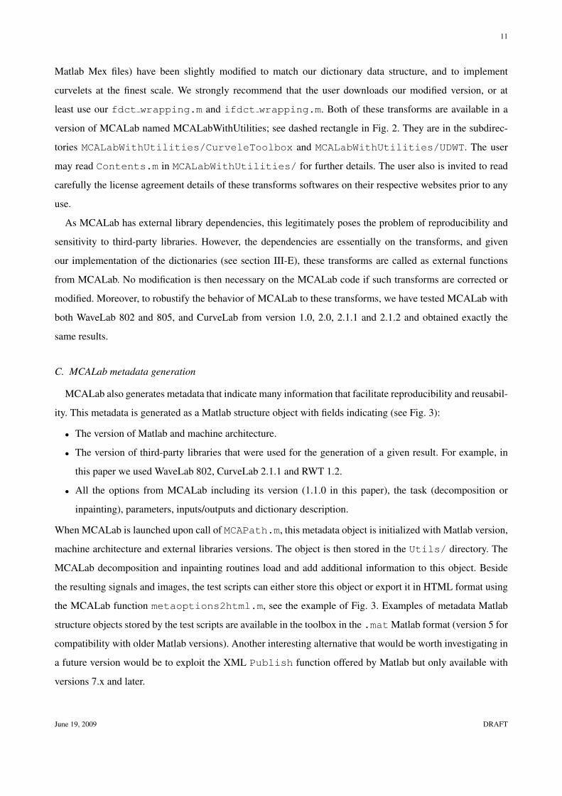
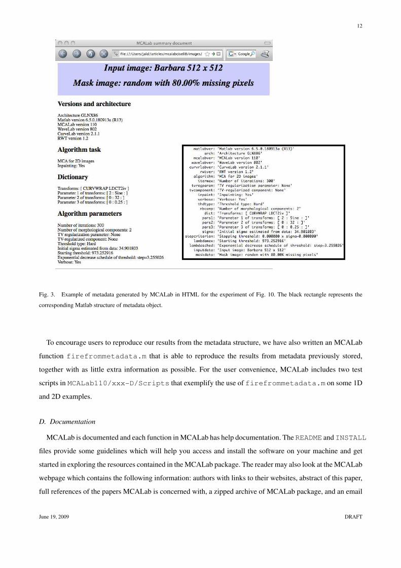
ity. This metadata is generated as a Matlab structure object with fields indicating (see Fig. 3):

• The version of Matlab and machine architecture.

• The version of third-party libraries that were used for the generation of a given result. For example, in

this paper we used WaveLab 802, CurveLab 2.1.1 and RWT 1.2.

• All the options from MCALab including its version (1.1.0 in this paper), the task (decomposition or

inpainting), parameters, inputs/outputs and dictionary description.

When MCALab is launched upon call of MCAPath.m, this metadata object is initialized with Matlab version,

machine architecture and external libraries versions. The object is then stored in the Utils/ directory. The

MCALab decomposition and inpainting routines load and add additional information to this object. Beside

the resulting signals and images, the test scripts can either store this object or export it in HTML format using

the MCALab function metaoptions2html.m, see the example of Fig. 3. Examples of metadata Matlab

structure objects stored by the test scripts are available in the toolbox in the .mat Matlab format (version 5 for

compatibility with older Matlab versions). Another interesting alternative that would be worth investigating in

a future version would be to exploit the XML Publish function offered by Matlab but only available with

versions 7.x and later.

June 19, 2009 DRAFT

12

Fig. 3. Example of metadata generated by MCALab in HTML for the experiment of Fig. 10. The black rectangle represents the

corresponding Matlab structure of metadata object.

To encourage users to reproduce our results from the metadata structure, we have also written an MCALab

function firefrommetadata.m that is able to reproduce the results from metadata previously stored,

together with as little extra information as possible. For the user convenience, MCALab includes two test

scripts in MCALab110/xxx-D/Scripts that exemplify the use of firefrommetadata.m on some 1D

and 2D examples.

D. Documentation

MCALab is documented and each function in MCALab has help documentation. The README and INSTALL

files provide some guidelines which will help you access and install the software on your machine and get

started in exploring the resources contained in the MCALab package. The reader may also look at the MCALab

webpage which contains the following information: authors with links to their websites, abstract of this paper,

full references of the papers MCALab is concerned with, a zipped archive of MCALab package, and an email

June 19, 2009 DRAFT

13

address for remarks and bug report. MCALab is under continuing development by the authors. We welcome

your feedback and suggestions for further enhancements, and any contributions you might make.

E. Dictionaries and data structures

The functions in xxx-D/Dictionary subdirectory provide fast implicit analysis and synthesis operators

for all dictionaries implemented in MCALab. It is worth noting that except for the FDCT with the wrapping

implementation [11], all dictionaries provided in MCALab are normalized such that atoms have unit ℓ2-norm.

The FDCT implements a non-normalized Parseval tight frame. Thus, a simple rule to compute the ℓ2-norm

of the atoms is 1/√

redundancy of the frame. Normalization has an important impact on the thresholding step

involved in the decomposition/inpainting engines. The thresholding functions coded in MCALab take care of

these normalization issues for the dictionaries it implements.

The data structure as well as the routines are inspired from those of Atomizer [19]. The dictionaries are

implemented in an object-oriented way. The top level routines are FastLA and FastLS. Each transform has

a fast analysis and a fast synthesis function named respectively FasNAMEOFTRANSFORMAnalysis and

FasNAMEOFTRANSFORMSynthesis. Four arguments (NameOfDict, par1, par2, par3) are used

to specify a dictionary. The meaning of each parameter is explained in the corresponding routine. Each

FasNAMEOFTRANSFORMAnalysis computes the transform coefficients (i.e. application of ΦT ) of an

image or a signal and stores them in a structure array. We also define the List data structure and corresponding

functions, which allow to create and easily manipulate overcomplete merged dictionaries. The interested user

can easily implement its own dictionary associated to a new transform following the above development rules.

F. Decomposition and inpainting engines

The routines in this directory perform either signal/image decomposition and inpainting using the MCA-

based Algorithm 1, or signal and image inpainting using Algorithm 2 described above. This set of routines are

for dictionaries with fast implicit operators. They are also designed so as to return a metadata object that can

be saved or exported in HTML format to facilitate result reproducibility.

G. Scripts and GUI

The makeup of /MCALab110/xxx-D/Scripts and /MCALab110/xxx-D/DemoGUI is the whole

raison d’etre of the MCALab toolbox. The subdirectory /MCALab110/xxx-D/Scripts contains a variety

of scripts, each of which contains a sequence of commands, datasets and parameters generating some figures

in our own articles, as well as other exploratory examples not included in the papers. One can also run the

same experiments on his own data or tune the parameters by simply modifying the scripts. By studying these

June 19, 2009 DRAFT

14

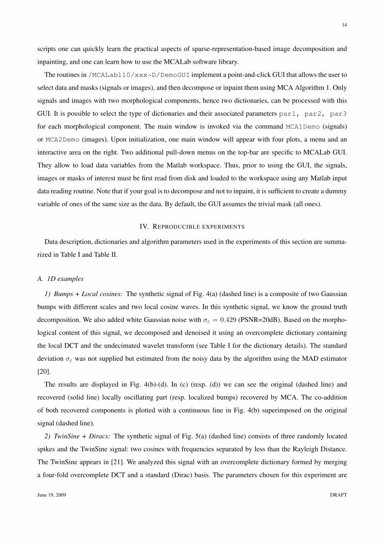
scripts one can quickly learn the practical aspects of sparse-representation-based image decomposition and

inpainting, and one can learn how to use the MCALab software library.

The routines in /MCALab110/xxx-D/DemoGUI implement a point-and-click GUI that allows the user to

select data and masks (signals or images), and then decompose or inpaint them using MCA Algorithm 1. Only

signals and images with two morphological components, hence two dictionaries, can be processed with this

GUI. It is possible to select the type of dictionaries and their associated parameters par1, par2, par3

for each morphological component. The main window is invoked via the command MCA1Demo (signals)

or MCA2Demo (images). Upon initialization, one main window will appear with four plots, a menu and an

interactive area on the right. Two additional pull-down menus on the top-bar are specific to MCALab GUI.

They allow to load data variables from the Matlab workspace. Thus, prior to using the GUI, the signals,

images or masks of interest must be first read from disk and loaded to the workspace using any Matlab input

data reading routine. Note that if your goal is to decompose and not to inpaint, it is sufficient to create a dummy

variable of ones of the same size as the data. By default, the GUI assumes the trivial mask (all ones).

IV. REPRODUCIBLE EXPERIMENTS

Data description, dictionaries and algorithm parameters used in the experiments of this section are summa-

rized in Table I and Table II.

A. 1D examples

1) Bumps + Local cosines: The synthetic signal of Fig. 4(a) (dashed line) is a composite of two Gaussian

bumps with different scales and two local cosine waves. In this synthetic signal, we know the ground truth

decomposition. We also added white Gaussian noise with σε = 0.429 (PSNR=20dB). Based on the morpho-

logical content of this signal, we decomposed and denoised it using an overcomplete dictionary containing

the local DCT and the undecimated wavelet transform (see Table I for the dictionary details). The standard

deviation σε was not supplied but estimated from the noisy data by the algorithm using the MAD estimator

[20].

The results are displayed in Fig. 4(b)-(d). In (c) (resp. (d)) we can see the original (dashed line) and

recovered (solid line) locally oscillating part (resp. localized bumps) recovered by MCA. The co-addition

of both recovered components is plotted with a continuous line in Fig. 4(b) superimposed on the original

signal (dashed line).

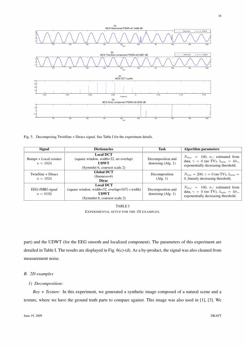
2) TwinSine + Diracs: The synthetic signal of Fig. 5(a) (dashed line) consists of three randomly located

spikes and the TwinSine signal: two cosines with frequencies separated by less than the Rayleigh Distance.

The TwinSine appears in [21]. We analyzed this signal with an overcomplete dictionary formed by merging

a four-fold overcomplete DCT and a standard (Dirac) basis. The parameters chosen for this experiment are

June 19, 2009 DRAFT

15

100 200 300 400 500 600 700 800 900 1000

−1

−0.5

0

0.5

1

Time

(a)Noisy signal PSNR

in=20 dB

100 200 300 400 500 600 700 800 900 1000−1

−0.5

0

0.5

1

Time

(b) Denoised MCA PSNR=38.1 dB

100 200 300 400 500 600 700 800 900 1000−1

−0.5

0

0.5

1

Time

(c)Local Cosines PSNR=39.9 dB

100 200 300 400 500 600 700 800 900 10000

0.2

0.4

0.6

0.8

Time

(d)Bumps PSNR=38.5 dB

Noisy

Original

Recovered

Original

Recovered

Original

Recovered

Original

Fig. 4. Decomposing and denoising Local sines + Bumps signal. See Table I for the experiment details.

summarized in Table I. The results are shown in Fig. 5(b)-(d). MCA managed to resolve the frequencies of

the oscillating (TwinSine (b)-(c)) component and to separate it properly from the spikes shown in (d). Al-

though some spurious frequencies are still present in the oscillating part. The locations of the true frequencies

correspond to the dotted lines in Fig. 5(c), and the original spikes are indicated by the crosses in Fig. 5(d).

3) EEG-fMRI: MCA was also applied to a real signal acquired during a multi-modal neuroimaging experi-

ment. During such an experiment, electroencephalography (EEG) and functional magnetic resonance imaging

(fMRI) data are recorded synchronously for the study of the spatio-temporal dynamics of the brain activity.

However, this simultaneous acquisition of EEG and fMRI data faces a major difficulty because of currents

induced by the MR magnetic fields yielding strong artifacts that generally dominate the useful EEG signal. In

a continuous acquisition protocol, both modalities are able to record data. But a post-processing step for EEG

artifact reduction is necessary for the EEG signal to be exploitable.

An example of such a signal1 is depicted in in Fig. 6(a). The periods where the MR sequence is switched

on are clearly visible inducing strong oscillations on the EEG signal with an amplitude 10 to 20 times higher

that the expected EEG amplitude. This locally oscillating behavior is expected because of the shape of the

magnetic field gradients of the MR scanner. Therefore, to get rid off of the MR component and clean the EEG

signal from these artifacts, we decomposed it using an overcomplete dictionary of local DCT (for the MR

1With courtesy of GIP Cyceron, Caen, France.

June 19, 2009 DRAFT

16

100 200 300 400 500 600 700 800 900 1000

−1

0

1

2

Time

(a) MCA Recovered PSNR=67.4488 dB

100 200 300 400 500 600 700 800 900 1000

−1

0

1

Time

(b) MCA TwinSine component PSNR=29.3687 dB

0.092 0.094 0.096 0.098 0.1 0.102 0.104 0.1060

10

20

30

40

Frequency

(c) MCA DCT coeffs

100 200 300 400 500 600 700 800 900 10000

0.5

1

1.5

2

Time

(d) MCA Dirac component PSNR=30.5055 dB

Recovered Original

Recovered Original

Fig. 5. Decomposing TwinSine + Diracs signal. See Table I for the experiment details.

Signal Dictionaries Task Algorithm parameters

Bumps + Local cosines

n = 1024

Local DCT

(square window, width=32, no overlap)

UDWT

(Symmlet 6, coarsest scale 2)

Decomposition and

denoising (Alg. 1)

Niter = 100, σε: estimated from

data, γ = 0 (no TV), λmin = 4σε,

exponentially decreasing threshold.

TwinSine + Diracs

n = 1024

Global DCT

(fineness=4)

Dirac

Decomposition

(Alg. 1)

Niter = 200, γ = 0 (no TV), λmin =

0, linearly decreasing threshold.

EEG-fMRI signal

n = 8192

Local DCT

(square window, width=32, overlap=50%×width)

UDWT

(Symmlet 6, coarsest scale 2)

Decomposition and

denoising (Alg. 1)

Niter = 100, σε: estimated from

data, γ = 0 (no TV), λmin = 4σε,

exponentially decreasing threshold.

TABLE I

EXPERIMENTAL SETUP FOR THE 1D EXAMPLES.

part) and the UDWT (for the EEG smooth and localized component). The parameters of this experiment are

detailed in Table I. The results are displayed in Fig. 6(c)-(d). As a by-product, the signal was also cleaned from

measurement noise.

B. 2D examples

1) Decomposition:

Boy + Texture: In this experiment, we generated a synthetic image composed of a natural scene and a

texture, where we have the ground truth parts to compare against. This image was also used in [1], [3]. We

June 19, 2009 DRAFT

17

500 1000 1500 2000 2500 3000 3500 4000−4000

−2000

0

2000

Time

(a) EEG−fMRI signal

500 1000 1500 2000 2500 3000 3500 4000−4000

−2000

0

2000

Time

(b) Denoised

500 1000 1500 2000 2500 3000 3500 4000−4000

−2000

0

2000

Time

(c) MCA MRI magnetic field induced component

500 1000 1500 2000 2500 3000 3500 4000

−100

−50

0

50

100

Time

(d) MCA EEG MRI−free component

Fig. 6. Decomposing and denoising the EEG-MRI real signal. See Table I for the experiment details.

Image Dictionaries Task Algorithm parameters

Boy + Texture

256× 256

Curvelets (cartoon)

(coarsest scale 2)

Global DCT (texture)

(low-frequencies removed)

Decomposition

(Alg. 1)

Niter = 50, γ = 0.1 (TV on car-

toon part), λmin = 0, exponentially

decreasing threshold.

Barbara

512× 512

Curvelets (cartoon)

(coarsest scale 2)

Decomposition

(Alg. 1)

Niter = 300, γ = 2 (TV on car-

toon part), λmin = 0, exponentially

decreasing threshold.

Local DCT (texture)

(sine-bell window, width=32, low-frequencies removed)

Inpainting

(Alg. 1-sec.II-D.1)

Niter = 300, γ = 0 (no TV), λmin =

0, linearly decreasing threshold

Risers 150× 501

Curvelets (lines)

(coarsest scale 2)

UDWT (smooth and isotropic)

(Symmlet 6, coarsest scale 2)

Decomposition and

denoising (Alg. 1)

Niter = 30, σε: estimated from data,

γ = 2 (TV on UDWT part), λmin =

3σε, exponentially decreasing thresh-

old.

Lines + Gaussians

256× 256

Curvelets (lines)

(coarsest scale 3)

Inpainting

(Alg. 1-sec.II-D.1)

Niter = 50, γ = 0 (no TV), λmin =

0, linearly decreasing threshold.

UDWT (Gaussians)

(Symmlet 6, coarsest scale 2)

Inpainting

(Alg. 2-sec.II-D.2)no noise, δ =1E-6, λ = 0.3.

Lena 512× 512Curvelets

(coarsest scale 2)

Inpainting

(Alg. 1-sec.II-D.1)

Niter = 300, γ = 0 (no TV),

λmin = 0, exponentially decreasing

threshold.

Inpainting

(Alg. 2-sec.II-D.2)no noise, δ =1E-6, λ = 10.

TABLE II

EXPERIMENTAL SETUP FOR THE 2D EXAMPLES.

June 19, 2009 DRAFT

18

used the MCA decomposition Algorithm 1 with the curvelet transform for the natural scene part, and a global

DCT transform for the texture; see Table II for details. The TV regularization parameter γ was fixed to 0.1.

In this example as for the example of Barbara to be described hereafter, we got better results if the very low-

frequencies were ignored in the textured part. The reason for this is the evident coherence between the two

dictionaries elements at low frequencies - both consider the low-frequency content as theirs. Fig. 7 shows the

original image (addition of the texture and the natural parts), the reconstructed cartoon (natural) component

and the texture part.

Barbara: We have also applied the MCA decomposition Algorithm 1 to the Barbara image. We used the

curvelet transform for the cartoon part, and a local DCT transform with a smooth sine window and a window

size 32× 32 for the locally oscillating texture. The TV regularization parameter γ was set to 2. Fig. 8 displays

the Barbara image, the recovered cartoon component and the reconstructed texture component.

Risers: The goal of this experiment is to illustrate the usefulness of MCA in a real-life application such

as studying the mechanical properties of composite risers used in the oil industry [22]. The top image of Fig. 9

displays a riser made of many layers that was recorded using a digital X-ray camera [22]. The riser is made

of a composite material layer, a layer of steel-made fibers having opposite lay angles, and lead-made markers

used as a reference to calibrate the X-ray camera. The structures of interest are the curvilinear fibers. But,

the markers that appear as black isotropic structures on the image, hide the fiber structures that exist behind

them. Our goal is to decompose this X-ray image into two components: one containing the curvilinear fiber

structures and the other with the lead-made markers and the smooth background. Therefore, natural candidate

dictionaries would be the curvelet transform for the fibers, and the UDWT for the isotropic markers and the

piecewise smooth background component. The TV penalty will be added to direct the image with the lead

markers to fit the piecewise smooth model with γ = 3. The image was also denoised by setting λmin = 3σε.

Fig. 9 illustrates the separation provided by the MCA. The top row depicts the original image, the middle and

bottom rows give the two components recovered by MCA. One can clearly see how it managed to get rid of the

lead-made markers while preserving the curvilinear fibers structure, and even reconstructing the unobserved

fibers parts that were behind the markers.

2) Inpainting:

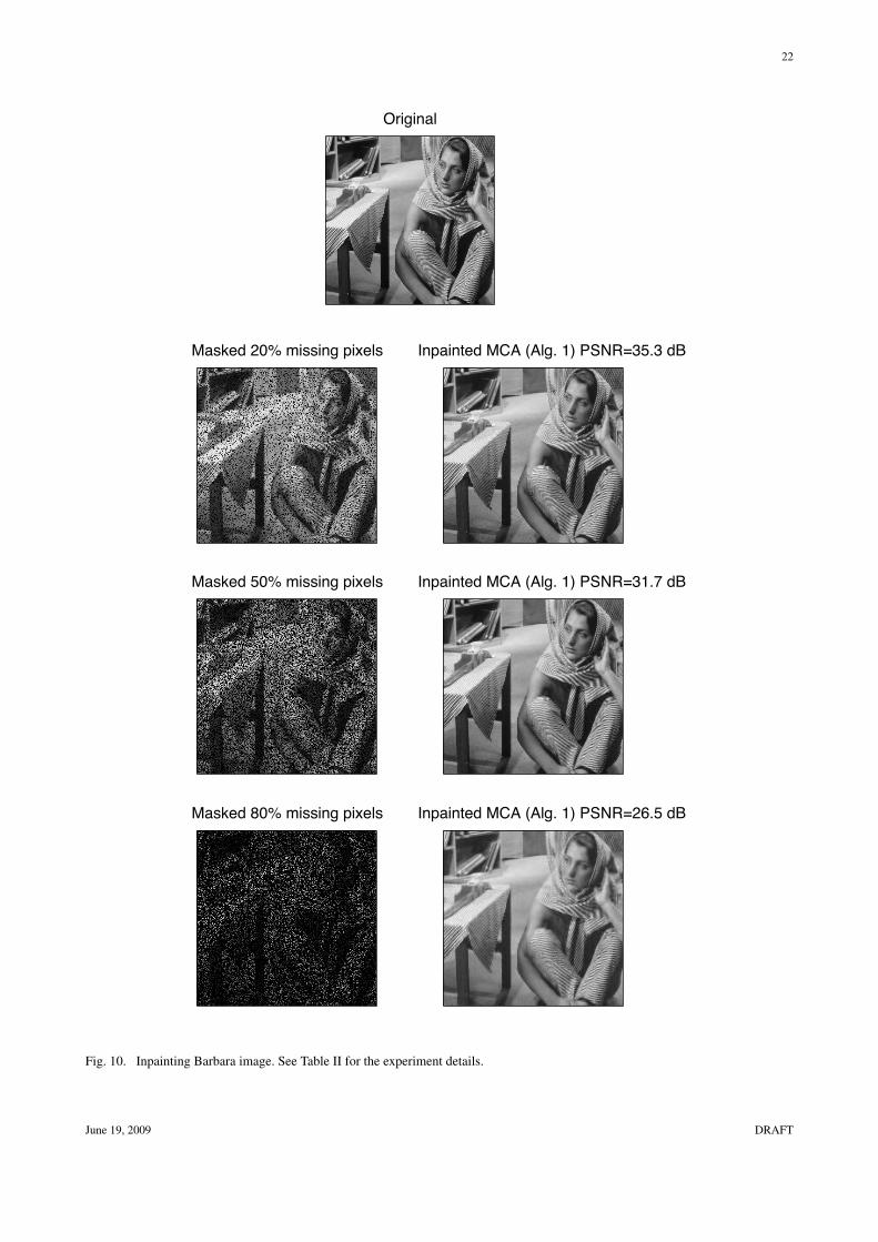
Barbara: Fig. 10 shows the Barbara image and its inpainted results for three random masks of 20%, 50%,

and 80% missing pixels. The unstructured random form of the mask makes the recovery task easier which is

intuitively acceptable using a compressed sensing argument [23], [24]. Again, the dictionary contained the

curvelet and local DCT transforms. The algorithm is not only able to recover the geometric part (cartoon), but

particularly performs well inside the textured areas.

Lines + Gaussians: We applied the two inpainting algorithms given in Algorithm 1-Section II-D.1 and

Algorithm 2-Section II-D.2 to a synthetic image which is a composite of three Gaussians and three lines, see

June 19, 2009 DRAFT

19

Original Texture + Boy Recovered MCA

Original Cartoon part MCA Cartoon

Original Texture MCA Texture

Fig. 7. Decomposing Boy-Texture image. See Table II for the experiment details.

June 19, 2009 DRAFT

20

Original Barbara MCA Barbara

Barbara Cartoon Barbara Texture

Fig. 8. Decomposing Barbara image. See Table II for the experiment details.

Fig. 11 top-left. Based on this morphological content, the UDWT and the curvelet transforms were chosen

as candidate dictionaries. The parameters chosen for each algorithm are summarized in Table II. The masked

and filled-in images are portrayed in Fig. 11. Both inpainting algorithm performed well, although the result of

Algorithm 2 is somewhat smoother.

Lena: We repeated the same experiment with Lena 512 × 512. The masked image is depicted in Fig. 12

top-right, where 80% pixels were missing, with large gaps. The dictionary contained the curvelet transform.

The parameters chosen for each algorithm are given in Table II. Despite the challenging difficulty of this

example (large gaps), both inpainting algorithms performed well. They managed to recover most important

details of the image that are hardly distinguishable by eye in the masked image. The visual quality is confirmed

by measures of the PSNR as reported in Fig. 12.

June 19, 2009 DRAFT

21

Original

MCA Isotropic and background

MCA Lines

Fig. 9. Decomposing Risers image. See Table II for the experiment details.

V. CONCLUSION AND FUTURE DIRECTIONS

Reproducible computational research remains an exception rather than a common practice in most pub-

lished papers of the image and signal processing community. In this paper, we described our experience

of reproducible research with MCALab, a complete software environment for sparse-representation-based

signal/image decomposition and inpainting. We described its architecture and discussed some results that

can be reproduced by running corresponding scripts in the MCALab package. Other exploratory examples

not included in the paper as well as a graphical user interface are also included in MCALab. We have

also recently released a C++ batch version of MCALab. It is available for download from the first author’s

webpage. The MCALab is under continuing development by the authors. Constructive feedback, suggestions

and contributions are warmly welcomed.

REFERENCES

[1] J.-L. Starck, M. Elad, and D. Donoho, “Image decomposition via the combination of sparse representatntions and variational

approach,” IEEE Trans. Image Process., vol. 14, no. 10, pp. 1570–1582, 2005.

[2] ——, “Redundant multiscale transforms and their application for morphological component analysis,” Advances in Imaging and

Electron Physics, vol. 132, 2004.

June 19, 2009 DRAFT

22

Masked 20% missing pixels Inpainted MCA (Alg. 1) PSNR=35.3 dB

Masked 50% missing pixels Inpainted MCA (Alg. 1) PSNR=31.7 dB

Masked 80% missing pixels Inpainted MCA (Alg. 1) PSNR=26.5 dB

Original

Fig. 10. Inpainting Barbara image. See Table II for the experiment details.

June 19, 2009 DRAFT

23

Original Lines + Gaussians Masked PSNR=30.9 dB

Inpainted EM (Alg. 2) PSNR=32 dB Inpainted MCA (Alg.1) PSNR=40 dB

Fig. 11. Inpainting Lines + Gaussians image. See Table II for the experiment details.

Original Lena Masked PSNR=6.44 dB

Inpainted EM (Alg. 2) PSNR=19.9 dB Inpainted MCA (Alg. 1) PSNR=19.9 dB

Fig. 12. Inpainting Lena image. See Table II for the experiment details.

June 19, 2009 DRAFT

24

[3] M. Elad, J.-L. Starck, P. Querre, and D. Donoho, “Simultaneous cartoon and texture image inpainting,” Appl. Comput. Harmon.

Anal., vol. 19, pp. 340–358, 2005.

[4] M. J. Fadili, J.-L. Starck, and F. Murtagh, “Inpainting and zooming using sparse representations,” Computer Journal, vol. 52,

no. 1, pp. 64–79, 2007.

[5] M. Schwab, N. Karrenbach, and J. Claerbout, “Making scientific computations reproducible,” Computing in Science and

Engineering, vol. 2, pp. 61–67, 2000.

[6] C. T. Silva and J. E. Tohline, “Computational provenance,” Computing in Science and Engineering, vol. 10, no. 3, pp. 9–10,

May./June. 2008.

[7] D. L. Donoho, A. Maleki, I. U. Rahman, M. Shahram, and Stodden, “Reproducible research in computational harmonic analysis,”

Computing in Science and Engineering, vol. 11, no. 1, pp. 8–18, Jan./Feb. 2009.

[8] M. Barni and F. Perez-Gonzales, “Pushing science into signal processing,” IEEE Signal Proc. Mag., vol. 22, pp. 119–120, 2005.

[9] Y. Meyer, “Oscillating patterns in image processing and in some nonlinear evolution equations.” The Fifteenth Dean Jacquelines

B. Lewis Memorial Lectures, 2001.

[10] S. G. Mallat, A Wavelet Tour of Signal Processing, 2nd ed. Academic Press, 1998.

[11] E. Candes, L. Demanet, D. Donoho, and L. Ying, “Fast discrete curvelet transforms,” CalTech, Applied and Computational

Mathematics, Tech. Rep., 2005.

[12] E. Candes and D. Donoho, “Ridgelets: the key to high dimensional intermittency?” Philosophical Transactions of the Royal

Society of London A, vol. 357, pp. 2495–2509, 1999.

[13] A. M. Bruckstein, D. L. Donoho, and M. Elad, “From sparse solutions of systems of equations to sparse modeling of signals and

images,” SIAM Review, vol. 51, no. 1, pp. 34–81, 2009.

[14] J. Bobin, J.-L. Starck, M. J. Fadili, Y. Moudden, and D. L. Donoho, “Morphological component analysis: An adaptive

thresholding strategy,” IEEE Trans. Image Process., vol. 16, no. 11, pp. 2675 – 2681, November 2007.

[15] http://www.cecill.info/index.en.html.

[16] J. Buckheit and D. Donoho, “Wavelab and reproducible research,” in Wavelets and Statistics, A. Antoniadis, Ed. Springer, 1995.

[17] Curvelab. [Online]. Available: http://www.curvelet.org

[18] Rice wavelet toolbox. [Online]. Available: http://www.dsp.rice.edu/software/rwt.shtml

[19] S. Chen, D. Donoho, M. Saunders, I. Johnstone, and J. Scargle, “About atomizer,” Stanford University, Department of Statistics,

Tech. Rep., 1995.

[20] D. L. Donoho and I. Johnstone, “Ideal spatial adaptation via wavelet shrinkage,” Biometrika, vol. 81, pp. 425–455, 1994.

[21] S. S. Chen, D. L. Donoho, and M. A. Saunders, “Atomic decomposition by basis pursuit,” SIAM Journal on Scientific Computing,

vol. 20, no. 1, pp. 33–61, 1999.

[22] D. Tschumperle, M. J. Fadili, and Y. Bentolila, “Wire structure pattern extraction and tracking from x-ray images of composite

mechanisms,” in IEEE CVPR’06, New-York, USA, 2006.

[23] E. Candes and T. Tao, “Near optimal signal recovery from random projections: Universal encoding strategies ?” IEEE Trans. Inf.

Theory, vol. 52, pp. 5406–5425, 2004.

[24] D. L. Donoho, “Compressed sensing,” IEEE Trans. Inf. Theory, vol. 52, no. 4, pp. 1289–1306, 2006.

June 19, 2009 DRAFT