CORPORATE FINANCE:AN INTRODUCTORY COURSE

DISCUSSION NOTES

MODULE #111

RISK AND RETURN: THE CAPITAL ASSET PRICING MODEL (CAPM)

I. Summary of Key Points:

The definition of risk is a major issue in finance. Risk is a "slippery" concept, i.e., it is not easy to define nor does it have a natural “unit.”

We assume that investors like expected return, E(r) (the more the better!), and dislike risk (the less the better!). In short, investors are risk averse--they must be compensated for bearing risk. Therefore, the relationship between expected (ex ante) return and risk must be upward sloping. After the fact, however, realized (ex post) returns can have upward, downward, or no relationship with risk. I will elaborate on this important distinction between expected and realized returns as a function of risk. However, over longer holding periods, return data, which we will discuss shortly, illustrate that risk has been rewarded historically with higher realized returns. We expect this for a long history.

Don’t ever think of E(r) without thinking about the risk associated with that E(r). Risk and return go together, like hand and glove! [Practice the following exercise in the shower every morning. Toss your bar of soap back-and-forth between hands and simultaneously say "risk versus return, risk versus return," where one hand with soap represents E(r) and the other hand with soap represents risk!] Okay maybe that’s a stupid thing to do but do whatever it takes to link these two words in your mind! High E(r) equates to high risk! If anyone tells you otherwise, beware! They are either a fool or a crook! Capital markets provide no (few?) free lunches, i.e., high returns with low risk!

II. E(r) and Volatility of Individual Securities:

The equation for the expected return on a security for time period t is

E(rt) = (E(Pt) - Pt-1 + E(Divt))/Pt-1.

Note again that the "E" represents expectations, or an expected but not realized value.Assume that at t = 0, today, a stock costs $60, or P0. This stock does not pay dividends. You expect one of the following three states of nature to occur in the next year:

1 This lecture module is designed to complement Chapters 11 and 12 in B&D.

1

Statei Probability of Statei P1i rti

Recession 1/3 $ 50-16.7%

Normal Times 1/3 $ 75 25.0%Boom Times 1/3 $100 66.7%

1.0

The expected price of the security at t = 1 isE(P1) = (1/3)*$50 + (1/3)*$75 + (1/3)*$100 = $75.

The expected return on the security in time period 1is E(r1) = (1/3)(-16.7%) + (1/3)(25.0%) + (1/3)(66.7%) = 25.0%, or

3E(r1) = Σ Probi*r1i, where

i=1

E(r1) is the expected return on the security in period 1, i indexes the three states that may occur, Probi = the probability of state i occurring, and r1i is the return on the security if state i occurs.

Note that the probabilities of the states must sum to 1.0.

Alternatively, we could calculate the expected return in one-period, E(r1), as above

E(r1) = (E(P1) - P0)/P0 = ($75 - $60)/$60 = 25.0% (note you still have to find E(P1)).

How might we measure the risk of the return over the coming year for this security? Candidate measures include:

Range of outcomes Variance of outcomes Standard Deviation of outcomes Other measures?

The range of outcomes is -16.7% to 66.7%. However, this measure lacks precision and lacks a relationship to the expected outcome. Further, probabilities of outcomes are not considered.

The variance of outcomes, σ2, is calculated as

N σ2 = Σ Probi(r1i – E(r1))2, where

i=1

2

i indexes the state i, N represents the number of possible states, Probi represents the probability of state i, r1i is the return in state i, and E(r1) represents the expected return over all states.

σ2 = (1/3)(-0.167 - 0.250)2 + (1/3)(0.250 - 0.250)2 + (1/3)(0.667 - 0.250)2

σ2 = 0.1159, or 11.59%2 in our numerical example.

The standard deviation of the outcomes, σ, is calculated as

σ = (σ2)1/2 or (0.1159)1/2 = 0.3405, or 34.05%.

Review the relationship of σ to the distribution of r1i's as per the material in an introductory statistics course, i.e., (+/-) 1 σ incorporates about 68% of the distribution centered on E(r), (+/-) 2σ incorporated about 95% of the distribution, (+/-) 3σ includes 99+% of the distribution, assuming the distribution is normally distributed.

The other possible measures of risk will be developed below.

A source of confusion is when to use Probi versus 1/N versus 1/(N-1) as the weight in the variance calculation, where N equals sample size. If all outcomes are equally likely, Probi = 1/N. Therefore, if all of the outcomes (here future states) are not equally likely, then 1/N is not appropriate to use as the weights in calculating the variance of a distribution--use Probi.

If you'll recall from your introductory statistics course, if you are analyzing actual realized data and the sample size is small, you should use 1/(N-1), when you have N observations, to correct for the small sample size bias problem. If the sample is large (N > 30), however, the sample size bias problem is negligible, using 1/N is a very close approximation.

III. Risk and Diversification--The Intuition:

Is the dispersion of the returns, actual or expected, measured by variance or standard deviation, the correct definition of risk for any single security? The answer is "yes" and "no."

The answer is "yes" if you are constrained to hold only one security. However, if you have the opportunity to diversify your assets, the answer is "no," variance is not a good measure of risk for a single asset. In our development of risk measures, we assume that the great majority of investors have the opportunity to diversify. Therefore, we must examine the impact diversification has on determining the appropriate measure of risk for an individual security.

What do we mean by diversification? Let's use an intuitive but extreme example.

We are examining an investment in two companies, The Umbrella Company, UC, and the Sun

3

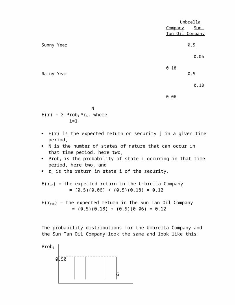
Tan Oil Company, STO. Details regarding these investments are as follows:

States of Nature Probability

Umbrella Company Sun Tan Oil Company

Sunny Year 0.5

0.06 0.18

Rainy Year 0.5 0.18 0.06

NE(r) = Σ Probi *ri, where i=1

E(r) is the expected return on security j in a given time period, N is the number of states of nature that can occur in that time period, here two, Probi is the probability of state i occuring in that time period, here two, and ri is the return in state i of the security.

E(ruc) = the expected return in the Umbrella Company = (0.5)(0.06) + (0.5)(0.18) = 0.12

E(rsto) = the expected return in the Sun Tan Oil Company = (0.5)(0.18) + (0.5)(0.06) = 0.12

The probability distributions for the Umbrella Company and the Sun Tan Oil Company look the same and look like this:

Probi

0.50

0.06 0.18 ri

Note that each security is risky, i.e., the realized return can be either 6% or 18%. A priori, you don’t know what outcome you will get in a given time period.

4

Now, let's create a portfolio of both stocks, with 50% of our investment capital invested in each company. The expected return for the portfolio, E(rp), is

5

SE(rp) = Xj*E(rj), where j=1

S = the number of securities in the portfolio, here two, Xj = weight of security j in the portfolio, here 0.5, andE(rj) = the expected return of each security (over all possible states, rain and sun), here 12% each.E(rp) = (0.5)(0.12) + (0.5)(0.12) = 0.12.

What is the risk of this portfolio return? The answer is zero as measured by dispersion. The probability distribution of returns on the portfolio looks like this:

Probi

1.00

0.12 E(r)In this example, you get a 12% return on your portfolio no matter what state of nature occurs. You are able to get this E(r) without any risk. Contrast this situation with what you get with either security alone, i.e, either 6% or 18% with equal probability.

This example is the general idea of how diversification works, when you hold several assets some do well and some do poorly, they tend to balance each other out. However, the above example is an extreme case. These two securities have a negative correlation, i.e., when one has high returns the other has low returns. How much risk reduction you get depends on the correlation of the returns on the assets included in the portfolio. Just how negative is the correlation between these assets in our example?

First, let's calculate the covariance between the two securities, or σus.

N σus = Σ Probi(ruci – E(ruc))*(rstoi – E(rsto)), where i=1

ruci and rstoi are the returns to the Umbrella Company and the Sun Tan Oil Company in state i, respectively, and E(ruc)and E(rsto) are the expected returns on these two firms over all states, respectively.

σus = (0.5)(0.06 - 0.12)(0.18 - 0.12) + (0.5)(0.18 - 0.12)(0.06 - 0.12)

6

σus = -0.0036.

Be able to discuss the intuition of what a covariance represents; just a review of the basic statistics course.

Recall the relationship between covariance, σus, and correlation, ρus.

ρus = σus/σucσsto.

We have calculated σus. The standard deviations, σuc and σsto, are both equal 0.06. (You should confirm these values!)

ρus = (-0.0036)/(0.06)(0.06) = -1.00.

Recall that all correlation coefficients, ρij, lie in the range -1.0, perfectly negative correlation, to +1.0, perfect positive correlation. The two firms that we have examined have perfect negative correlation. In this situation, it is possible to choose weights for the securities, Xu and Xs, which will drive the standard deviation of the portfolio to zero.

Since we have assumed that investors like E(r) and dislike risk, it is natural for them to seek diversification in their investments. Diversification implies that total risk decreases as you add securities to your portfolio.

While perfect negatively correlated securities allow you to eliminate risk completely, you can reduce risk with any pair of securities as long as the correlation is less than +1.0. However, the less correlated the better in terms of their diversification impact.

Based upon the above example, you should be beginning to see why the variance or standard deviation of a security is not a good measure of the risk of the security. With diversification, much of this standard deviation risk can be eliminated. This brilliant insight was first recognized by Professors Harry Markowitz and James Tobin. For their contributions in the fields of economics and finance both were awarded Nobel Prizes in Economics. What is the bottom line of this observation? Don't put all of your eggs in one basket! Yes, but they demonstrated it rigorously.

IV. Risk and Diversification--The Formalities:

The expected return on a portfolio is

S E(rp) = Σ XjE(rj), where j=1

S is the number of securities in the portfolio, Xi is the dollar value proportion of Security i in the portfolio, which must sum to 1.0,

7

and E(rj) is the expected return on Security j.

E(rp)'s are easy to calculate; they are just the weighted average of the component security returns.

Example:

You plan to combine Security A with Security B into a portfolio using 20% of your funds to buy A and 80% of your funds to buy B. Securities A and B have expected returns of 10% and 12%, respectively.

E(rp) = (0.20)(0.10) + (0.80)(0.12) = 0.116, or 11.6%. Nothing to it, right?

Unfortunately, the variance or standard deviation of a portfolio is not quite so easy. The equation for the variance of a portfolio is as follows:

S S σ2

p = Σ Σ XiXjσij, where i=1 j=1

S equals the number of securities in the portfolio, Xi and Xj are the weighs of securities i and j, respectively, and σij is the covariance between i and j.

Be able to discuss in detail what the above equation represents and how it works!

Given the relationship between covariance and correlation, an alternative way to write the above equation is

S S σ2

p = Σ Σ XiXjρijσiσj. i=1 j=1

All we've done is substitute ρijσiσj = σij. (Remember, ρij = σij/σiσj.)

The variance equation for a portfolio looks pretty intimidating, doesn't it? However, let's start with the simplest case, the case of a two-security portfolio, and it won't seem so bad.

The Case of Two Securities:

For two securities, the portfolio variance equation in terms of σij looks like this:

σ2p = X2

1σ21 + X1X2σ12 + X2X1σ21 + X2

2σ22.

Since σ12 equals σ21 (the covariance of security 1 with security 2 equals the covariance of security 2 with security 1), and X1X2 equals X2X1, we can write the middle two terms as 2X1X2σ12. (Of course, we could also write them 2X2X1σ21.)

8

For two securities, the portfolio variance equation in terms of ρij looks like this:

σ2p = X2

1σ21 + X1X2ρ12σ1σ2 + X2X1ρ21σ2σ1 + X2

2σ22.

Again, the two middle terms are equal and can be written 2X1X2ρ12σ1σ2.

Let's work through an example to make this expansion clear.

State Prob r1 r2

1 0.20 0.07 0.12 2 0.60 0.12 0.10 3 0.20 0.17 0.08

At this point, you should be able to calculate the E(r)’s for both securities 1 and 2; they are 0.12 and 0.10, respectively. You should also be able to calculate the variances for assets 1 and 2 as 0.0010 and 0.00016, respectively. Their standard deviations are 0.03162 and 0.01265, respectively. The covariance of the returns on asset 1 with the returns on asset 2, σ12 equals -0.0004.

Therefore, the correlation between 1 and 2, ρij, equals -1.0. (Check my math!)

Now, suppose we want to know the portfolio expected return and variance if we put 30% of our funds in Security 1 and 70% in Security 2.

E(rp) = (0.30)(0.12) + (0.70)(0.10) = 0.10 = 10.6%

Using the covariance version of the portfolio variance equation, we have

σ2p = (0.30)2(0.0010) + 2(0.30)(0.70)(-0.0004) + (0.70)2(0.00016)

σ2p = 0.00.

Here is another look at our example of being able to "squeeze" all of the risk out of a portfolio if the correlation is perfectly negative, -1.0.

Using the correlation based version of the portfolio variance equation, we have

σ2p = (0.30)2(0.0010) + 2(0.30)(0.70)(-1.0)(0.03162)(0.01265) + (0.70)2(0.00016) = 0.0.

Unfortunately, correlations between securities are usually positive. Security returns tend to move together to some degree. Finding perfectly negatively correlated securities (outside of the derivative markets) would be a very rare event.

Let's look at three cases where pairs of securities have correlations of +1.00 (perfectly positive), -1.00 (perfectly negative), and 0.00 (no correlation). These examples include

9

the "end points" of the correlation range, as well as the midpoint of this range. We will be putting together three portfolios of two stocks each with weights of X1 and X2. Of course X1 + X2 = 1.00 since the sum of the weights of securities in a portfolio must sum to 100% of the portfolio.

Case #1: Correlation, ρ12, = +1.00

E(rp) = X1E(r1) + X2E(r2). This equation represents a straight-line (linear) relationship between the two securities relative to the vertical axis, E(rp) (see figure 10.4 in RWJ).

σ2p = X2

1σ21 + 2X1X2ρ12σ1σ2 + X2

2σ22

Since ρ12 = +1.0, we have

σ2p = X2

1σ21 + 2X1X2σ1σ2 + X2

2σ22. This expression can be factored as

σ2p = (X1σ1 + X2σ2)2.

The standard deviation of this expression is

σp = (X1σ1 + X2σ2). Again, this equation represents a linear relationship between the two securities relative to the horizontal axis, σp.

Given these linear relationships, can you illustrate the graph of E(rp) and σp possibilities using securities 1 and 2 by varying the weights of the two securities in the portfolio?

By combining two securities with perfectly positive correlation, we get risk averaging, not risk reduction. Risk and return are just proportional to the amounts of each security in the portfolio. The portfolio's risk (standard deviation of return) is a linear function of the weights of the securities in the portfolio, X1 and X2.

Case #2: Correlation, ρ12, = -1.00

E(rp) = X1E(r1) + X2E(r2), as before.

σ2p = X2

1σ21 + 2X1X2ρ12σ1σ2 + X2

2σ22. Since ρ12 = -1.0, we have

σ2p = X2

1σ21 - 2X1X2σ1σ2 + X2

2σ22. This expression can be factored as

σ2p = (X1σ1 - X2σ2)2.

The standard deviation of this expression is

σp = (X1σ1 - X2σ2). Again, this is a linear relationship.

Given σ1 and σ2, it is possible to choose X1 and X2 in such a way as to eliminate all risk,

10

or so to get σp = 0. Remember that X1 + X2 must = 1.0.

Example: Say σ1 = 0.20 and σ2 = 0.40. These parameters can be calculated from observable data. Assume that ρ12, = -1.00, this is also a parameter that can be calculated from observable data.

Under these conditions, can σp = (X1σ1 - X2σ2) = 0? If so,

X1σ1 = X2σ2.

X1/X2 = σ2/σ1. Since we know σ1 and σ2, we can calculate the ratio as 0.40/0.20 = 2.0. Therefore, X1/X2 = 2.0. Therefore, X1 = 2.0*X2.

Since X1 + X2 =1.0, substituting from above, we know 2.0*X2 + X2 = 1.0.

Therefore, X2 = 1/3 and X1 must = 2/3. These are the portfolio weights that will create a portfolio with zero standard deviation. For example, if you have $12,000 to invest, you would put $4,000 in Security 2 and $8,000 in Security 1.

[Check: Does X1σ1 - X2σ2 = σp = 0.00? (2/3)(0.20) - (1/3)(0.10) = 0. Therefore, these weights do reduce the portfolio standard deviation (and so its variance) to zero.]

If ρ12 = -1.0, illustrate the following relationship in E(r) and standard deviation space by varying the weights on the two securities.

By combining two securities with perfectly negative correlation, we can completely eliminate risk by the appropriate choice of X1 and X2. Remember--the investor chooses the X's (portfolio weights) in his/her portfolio. With perfectly negative correlation, we have diversification at its best!

Case #3: Correlation, ρ12, = 0.00

E(rp) = X1E(r1) + X2E(r2), as before.

σ2p = X2

1σ21 + 2X1X2ρ12σ1σ2 + X2

2σ22. Since ρ12 = 0.0, we have

σ2p = X2

1σ21 + X2

2σ22

σp = (X21σ2

1 + X22σ2

2)1/2

Given the "squared" terms, we know that this relationship is quadratic, or a curved relationship. The curve will "bulge" to the left. Why? The σp will be less than when ρ is +1.0, but more than when ρ is -1.0; the curve will fall between these limiting cases.

Show Case #3 graphically. Again figure 10.4 in RWJ does this for you but understand it.

11

The implications of these three cases, where ρ is +1.0, -1.0, and 0.0, illustrate that diversification reduces risk if, and only if, the correlation is less than +1.0. You simply get risk averaging if the correlation is +1.0. With correlations less than +1.0, you get risk reduction, the lower the correlation, the greater the risk reduction (i.e., the greater the "bulge" to the left).

The Case of Many Securities:

Recall the equation for the expected return on a portfolio,

S E(rp) = Σ XiE(ri), where i=1

S is the number of securities in the portfolio, Xi is the dollar value proportion of security i in the portfolio, and E(ri) is the expected return on security i.

E(rp)'s continue to be easy to figure for large portfolios, they are just the weighted average of the component security returns. Unfortunately, the variance or standard deviation of a portfolio gets "messier" than in the two-security case.

Again, the equation for the variance of a portfolio in terms of covariance is as follows:

S S σ2

p = Σ Σ XiXjσij, where i=1 j=1

S equals the number of securities in the portfolio, Xi and Xj are the weighs of securities i and j, and σij is the covariance between i and j. (Again, we could substitute ρijσiσj for the

covariance term.)

Write out the above variance expression for three securities.

Thinking of the above variance equation for a large portfolio in terms of a covariance matrix is useful. For a portfolio of size S, the above equation has S2 terms. Think of the equation in terms of a S x S matrix as below.

12

COVARIANCE MATRIX

σ21 σ 12 σ13 ... ... ... σ1S

σ21 σ 22 σ23 ... ... ... ...

σ31 σ 32 σ23 ... ... ... ...

... ... ... ... ... ... ...

... ... ... ... ... ... ...

... ... ... ... ... ... ...

S1 ... ... ... ... ... σ2S

In this matrix, we have S2 cells. S of these cells are occupied by variance terms; these terms are the diagonal cells from the northwest to the southeast corner of the matrix. S2 - S of the cells, or the remaining cells, are occupied by covariance terms. Note, however, that the "off-diagonal" cells have equal values, e.g., σ12 = σ21, σ13 = σ31, etc. This covariance matrix can easily be converted to a correlation matrix. How?

As S gets very large, the impact of the variance terms on the total risk of the portfolio gets smaller and smaller; the impact of the covariance terms gets larger and larger.

To keep it simple and illustrate this point, assume the securities all have equal variances, VAR. Further assume that all of the covariances between pairs of securities are equal, or COV, and that the weights are all equal so Xi = 1/S.

σ2p = S(1/S)2(VAR) + (S2 - S)(1/S)2(COV).

· If S = 10, σ2p = 0.10(VAR) + 0.90(COV).

· If S = 100, σ2p = 0.01(VAR) + 0.99(COV).

· If S = 1000, σ2p = 0.001(VAR) + 0.999(COV).

The detail to remember is that as portfolios have more and more assets, the variance (or standard deviation) of securities becomes less and less important and the covariance of the security with all other securities in the portfolio becomes more and more important. This observation is additional evidence that a security's variance or standard deviation is not its relevant measure of risk when an investor has the ability to form portfolios (i.e. diversify).

A key point: The positive covariances in the market set the limits of diversification.

If investors dislike risk, they will design portfolios that minimize σp for a given E(rp). What is important is the security's covariance risk in a portfolio, not its individual total risk, σ2

i, or σi.

Markowitz developed a procedure to select the "best" portfolios from all possible permutations and combinations of portfolios chosen from a set of S individual securities. We discuss the definition of "best" next.

13

V. Portfolio Theory:We now have the tools (equations) to calculate the E(rp) and σp of portfolios. (Note: it is critical that you are comfortable in making the basic calculations!)

Imagine that you have assembled a database with S securities. For each of these securities you have an estimate of its E(ri), its σi, and its covariance with each of the other S-1 securities, σij. Upon inspection, you quickly realize that all of your securities have positive covariances with the other securities. Accordingly, your opportunity to construct portfolios with zero variance, or standard deviation, is not available.

Now, assume that you throw darts at a listing of your S securities. Let's assume that you had 500 securities in your data set. You begin to randomly form portfolios, from sizes of one security each (not really a portfolio!) up to all S securities. You also throw darts at a list of proportions for each security to have in each portfolio, from proportions ranging from 0.00 to 1.00. Of course, the weights for an individual portfolio are properly constrained to sum to 1.0. (Do you understand why?)

You soon grow very tired of throwing darts. You next calculate the E(rp) and σp of each of your portfolios. You then plot your results in E(rp) and σp space. Illustrate the results of this exercise graphically.

It's a mess, right? How can we make any possible sense of this graph? Dr. Markowitz's procedure (a quadratic programming model) is as follows:

Minimize σ2p, subject to two conditions:

E(rp) is a constant (solve the problem for a range of values), and

S Σ Xi = 1. i=1

This model will trace out the "efficient set of risky portfolios" or the set of "efficient risky portfolios" from among all possible permutations and combinations of securities and weights. The model determines the Xi's for each security that appears in an individual efficient portfolio. Obviously, you need a computer to accomplish this task! See your text for an illustration of the efficient set of portfolios with a graph.

Note that only efficient risky portfolios are included on the efficient set. These efficient portfolios must satisfy two criteria:

· For a given E(rp) they have minimum σp.

· For a given σp they have maximum E(rp).

14

In words, for each E(rp) only one minimum σp portfolio exists. For each σp, only one maximum E(rp) portfolio exists. These are efficient portfolios.

Be able to discuss why we ignore or "throw away" portfolios on the efficient set that lie below the minimum variance point. (If you draw vertical lines through the efficient set, for portfolios below than the minimum variance point, you will find another efficient portfolio above it with a higher E(rp) and the same risk. In other words, portfolios below this point on the efficient set are “dominated,” no one wants them, by efficient portfolios that lie above it on the efficient set and have the same risk, σp. Thus we ignore them.)

Key Questions:

Why does the efficient set of portfolios "bulge" to the left? (Hint: Recall the results of our investigation of two asset portfolios with +1.0, -1.0, and 0.00 correlation.)

Why doesn't the efficient set of portfolios intersect the E(rp) (or the y) axis? (Hint: you can only completely eliminate risk if you have securities with perfectly negative corrleation.)

How would estimating and using the set of efficient portfolios work in the "real world?"

Steps:

1) Security analysts would provide estimates of E(ri)'s, σi's, and σij's.

2) Portfolio managers would take these inputs, use Markowitz's quadratic programming procedure, and compute the efficient set. Again, note that the outputs from the computer algorithm are the set of securities to select for each efficient portfolio along with the weights, Xi's, for each security in the individual efficient portfolio. The model effectively "traces out" the efficient set of portfolios.

3) Investment advisors then present the efficient set to investors. Based upon their own tastes and preferences, i.e., their aversion to risk, investors "pick" an efficient portfolio that meets their needs. Note that each investor has the opportunity to choose a unique portfolio. As long as the portfolio is a member of the efficient set, i.e., on the "curve," it is an optimal portfolio for that risk level.

What efficient portfolio would you choose? That is a personal decision. You consider your own “tastes and preferences” for risk versus return in making your choice. You must decide if you want to "eat well or sleep well!" No one can tell you which efficient portfolio is best for you! But, once again, whichever portfolio you choose must be an efficient set portfolio if you are risk-averse.

Now that we have explained the rationale for why intelligent, risk-averse investors want to diversify, and how the most efficient diversification can be achieved, the question is how the

15

"small" investor can achieve this diversification. Given the high brokerage commissions on small trades, is diversification practically achievable for most of us?

Fortunately, the answer is yes! Even small investors can invest in well-diversified mutual funds with initial investments as small as $1000 or less and subsequent deposits as small as $50 per month. If you buy a "no load" mutual fund you do not even have to pay sales commissions. A "no load" mutual fund has no sales people; you have to write or call the mutual fund for a prospectus, fill out an application, and mail in your initial investment. The prospectus explains the investment philosophy and goals of the fund.

All types of mutual funds are available, from funds that invest in T-Bills, commercial paper, and other money market instruments, i.e., money market funds, to those that specialize in specific industries, sector funds, to those that invest only in stocks in a particular country, e.g., Japan. You can even buy an "index fund," or a fund that just duplicates an investment in an index, such as the S&P 500.

Since mutual funds are large institutional investors and trade in large blocks of stock, they have much lower transaction costs per trade than the small trader realize. Therefore, mutual funds are a low cost and practical way for the small investor to begin building an investment portfolio and, if selected appropriately, achieve "instant" diversification.

A publication available in the reference section of most libraries, Wiesenberger Investment Companies Service, summarizes the types of funds, commissions charged, management fees charged, risk, etc., along with contact information.

Consensus Opinions:

Now, imagine a world, as far-fetched as it may seem, where all investors have the same estimated values for E(ri)'s, σi's, and σij's. If these estimates indeed are all the same, how many efficient sets of risky portfolios would exist?

The answer is one (1), which will be explained shortly! If all of the input estimates are equal, every portfolio manager would come up with exactly the same efficient set of risky portfolios. This conclusion has to be true because the location and shape of the efficient set is determined by the input measures, which we've just assumed to be the same for everyone.

Obviously, every investor will not come up with the same estimates; many different estimates of the efficient set will exist at a given time. However, in aggregate, one consensus efficient set will dominate. This aggregate consensus efficient set would function as the "market's" efficient set, or as though all investors used the same security estimates. Accordingly, this "consensus" market efficient set is determined as though investors had homogeneous expectations, a fancy term for investors having the same estimates of E(ri)'s, σ's, and σij's. We will have more to say about the concept of homogeneous expectations later.

VI. Does Diversification Work?

16

Let's take the data that we discussed above for 500 stocks. Now randomly choose 30 single stocks and compute the standard deviations for each security for this group. Then average these standard deviations. Next, randomly choose 30 two-stock portfolios and calculate the standard deviation for each portfolio. Then average the 30 portfolio standard deviations. Repeat the above for 30 three-stock portfolios, 30 four-stock portfolios, etc., until you've completed thirty 30-stock portfolios.

Next, plot your results using average σp for each portfolio size as your y-axis and the number of stocks in the portfolio as your x-axis. Illustrate the results with a diagram (figure 10.7 in RWJ).

Note that "Total Portfolio Risk" for a given portfolio size,

σp = "Market Risk" + "Unique Risk."

Also note that the unique risk gets smaller and smaller as the portfolio size gets larger and larger. Finally, note that adding more securities to portfolios that have more than 30 randomly chosen stocks does not significantly contribute to further risk reduction.

When all possible "unique or unsystematic or diversifiable" risk has been "squeezed" out of a portfolio, the investor is still left with "market or systematic or nondiversifiable" risk.

To recap what we discussed above, for the investor that selects a diversified portfolio, the total risk, σi, of security i is not important. What is important is the security's risk that cannot be diversified away. This is the security’s contribution to the risk of a diversified portfolio. This risk is represented by the security's covariance risk with the other securities in the portfolio.

VII. Efficient Risky Portfolios Plus the Risk-Free Asset:

One of Markowitz's Ph.D. students, William Sharpe, extended his Professor's work by considering the risk-free asset in combination with the efficient set of risky portfolios. Let's re-visit our graph of the efficient set using the axes E(rp) and σp. Further, let's assume homogeneous expectations on the part of investors; therefore, only one efficient set exists.

Add the risk-free rate, rf to the efficient set diagram, or the point on the vertical, E(rp), axis with zero risk, or σ = 0. Think of the risk-free asset as a Treasury Bill. Now, using this point, rf, as the origin, draw a line that is tangent to the efficient set of risky portfolios. Illustrate this procedure graphically (figure 10.9 in RWJ).

Of course you could have drawn other straight lines from rf to points on the efficient set curve. Which of these lines is best? If you're a risk averse investor, you want the steepest possible sloped line. Why? You like E(r) and you dislike risk, σp. Therefore, the line with the largest slope is the preferred line; this line has the most E(r) per unit of risk. However, you are limited in your search for the steepest line by the location of the efficient set of risky portfolios. The tangency point, M, from rf to the efficient set of risky assets is the best you can do, i.e., the highest slope possible.

17

The line through the tangency portfolio, M, is of special significance. This line represents the new efficient set of all assets, risky and risk-free. Note for any level of risk, portfolios formed by combining the risk-free asset and portfolio M dominate all other risky portfolios on the efficient set of just risky portfolios, i.e., have higher E(rp). Alternatively, for any level of E(rp), all portfolios on the line dominate the set for risky portfolios by having lower risk (except for Portfolio M, of course).

Adding the risk-free asset in combination with the efficient set of risky portfolios was a brilliant insight. But why is the relationship between the risk-free asset and Portfolio M linear? It is because the σrf is zero and the covariance of M and rf equals zero.

Example:

Assume that the expected return on T-Bills is 7.0% and the expected return on M is 16%. What is the E(rp) consisting of 30% invested in T-Bills and 70% in M? Using our equation for the E(rp) we have:

E(rp) = (0.3)(0.07) + (0.7)(0.16) = 0.133.

What about the variance of the portfolio that we've described above? Assume that the variance of returns of M is 0.044 (standard deviation = 0.21) and the variance of the risk-free rate is zero. Using our equation for σ2

p we have:

σ2p = (0.3)2(σ2

rf) + (2)(0.3)(0.7)(σrf,m) + (0.7)2(σ2m)

= (0.09)(0) + (0.42)(0) + (0.49)(0.044) = 0.0256.

σp = 0.147.

Since the first two terms drop out (T-Bills have zero risk and zero covariance with M), the variance of the portfolio is just the weight invested in M squared times the variance of M. The standard deviation of the portfolio is

σp = Xmσm, or (0.7)(0.21) = 0.147.

Therefore, the E(r) versus risk (σp) relationship of the risk-free asset and M is a linear relationship in our picture.

Our new efficient set now extends on a straight line between rf and M in E(r) and σp space.

If we invest 100% of our assets in T-Bills, we find ourselves at rf with zero risk. If we invest 100% of our assets in M, we have an expected return of E(rm) and risk of σm. By putting some of our money in T-Bills and some of our money in M, we can position ourselves anywhere on the line between rf and M.

18

When we invest some (or all) of our money in T-Bills we are actually "lending" money to the U.S. Government. Therefore, any position below M on the line (but excluding M) is considered to be a "lending portfolio."

Moreover, we can actually move up a linear extension of the rf to M line past M by borrowing money and investing our own money plus the borrowed money all in Portfolio M--a "borrowing portfolio."

Example:

Suppose you have $1,000 invested in M. Using this investment as collateral, you borrow $500 which you also invest in M. Assume that you can borrow at the rate rf. What is your E(rp) and risk, σp?

Using the numbers from the last example, we have:

E(rp) = (1.5)(0.16) - (0.5)(0.07) = 0.205.

For every $1 of our money, we have $1.50 invested in M. Hence, the first component of the equation is (1.5)(0.16). However, for every $1.50 invested we've borrowed $0.50. We must pay interest on this loan at 7%. This repayment of interest represents the second term, -(0.5)(0.07). We have "levered up" the E(rm) from 16% to 20.5% by borrowing and investing everything in M. (NOTE: X1 + X2 = 1.5 + (-)0.5 = 1.0!)

Have we created a money machine? By borrowing and investing in Portfolio M you have higher expected return yes but also a higher risk level than the "pure" market risk, or σm = 0.21. The risk of our "levered" portfolio is

σp = (Xm)(σm) = (1.5)(0.21) = 0.32, where Xm is the weight invested in Portfolio M. Note the substantial increase in risk necessary to get the higher "levered" expected return. More risk, more expected return! No "free lunch" here!

Illustrate the straight line from rf through M and extended beyond M.

Once again, the separation point between the “lending” and “borrowing” portfolio is M. The resulting line extending from rf through M and onward is called the Capital Market Line, CML. Note the risk measure that is relevant for portfolios that lie on the CML, efficient portfolios, is σp. This is the relevant measure of risk for efficient portfolios.

VIII. What is Portfolio M?

Given homogeneous expectations, all investors want to hold Portfolio M in some combination with the risk-free asset (unless, of course, they want all of their money in T-Bills!). Investors adjust for risk by the percentage held in T-Bills. Lending or borrowing equals being long (owning) or short (borrowing) T-Bills. The long/short position in T-Bills in combination with

19

the ownership percentage of M determines the investor’s risk level. In short, M is a very special portfolio!

To review once again, all investors that are willing to hold some risk in their investment portfolio want to hold M to some degree. All assets must be held (if no one wants to hold, or own, an asset, it isn't much of an asset is it?). Therefore, Portfolio M must represent the portfolio of all assets. These assets, of necessity, must be held in market value proportions. Does this logic make sense?

Example:

Imagine that only four risky assets exist in the economy, Assets A, B, C, and D. Let's say that the total market value of A is $1,000. Similarly, B, C, and D have total market values of $750, $500, and $250, respectively. The total value of the market portfolio, M, the sum of all risky assets in the economy, is $2,500 ($1,000 + $750 + $500 + $250). Everybody wants to hold some of M. Why? The line defined by M and the risk-free asset represents the efficient set of assets, the best risk/return tradeoff you can find.

Further, imagine that the economy has only 10 investors, each with $250 they wish to invest in M plus additional amounts they wish to invest in T-Bills (long or short) to adjust for their personal risk preferences. How will they go about investing in M?

Since 40% of the Market Portfolio, M, is made up of security A ($1,000/$2,500), each investor will invest (40%)($250) of his/her money in Security A, or $100. Similarly, each investor will invest 30% of their money in B, 20% in C, and 10% in D. Each investor has invested their $250 in "market value proportions." Each investor effectively holds the market portfolio on a "scaled-down" basis.

IX. The Capital Market Line (CML):

Let's now write out an equation for the straight line beginning at rf and extending through the Market Portfolio, M, and beyond. Recall the equation for a general straight line is

y = b + mx, where

y is the unit of measure on the y-axis, b is the intercept on the y-axis, m is the slope of the line, and x is the unit of measure on the x-axis.

By inspection of the previous diagram, the equation of interest to us is as follows:

E(rp) = rf + [(E(rm) - rf)/σm]σp.

Relate the above equation to the equation for a straight line. This equation traces out what we have labeled the Capital Market Line (CML). The CML represents the location of all efficient

20

portfolios! The slope of this line is (E(rm) - rf)/σm.

Note the measure of risk for an efficient portfolio is σp! Again, this observation is very important for what follows.

X. Capital Market Theory:

Let's go back to our efficient set of risky portfolios, or the efficient set before we introduced investments combining the optimal risky portfolio, M, with the risk-free asset.

Calculating the Markowitz efficient set of risky portfolio is elegant but has one major problem--it's too much work! Think about how many estimates the security analyst has to make in order to satisfy the data needs for the efficient set:

· S estimates of E(ri)'s,· S estimates of σ2

i's,· (S2 - S)/2 estimates of "unique" covariance terms, σij's.

For example, a portfolio of 100 securities would require 5,150 unique estimates (100 + 100 + (1002 - 100)/2 = 5,150). Accordingly, while Markowitz's portfolio theory and efficient set procedure was much admired, it was little used because of the enormous data requirements. (Plus, and a BIG plus, they didn’t have ready access to affordable computers in those days!)

Besides his insight of adding the risk-free asset to the Markowitz's efficient set of risky portfolios, Professor William Sharpe further refined Markowitz's Model to make the estimation requirements and computations more feasible. For the significant extensions he made to Markowitz's Portfolio Theory, Professor Sharpe was awarded the Nobel Prize in Economics himself. Ironically, he was awarded this honor jointly with Markowitz in the same year—1990

Sharpe's idea was to relate all securities to the risk of the Market Portfolio rather than deal with all of the covariance terms necessary to develop the efficient set. In other words, Sharpe's insight eliminated the necessity for the (S2 - S)/2 covariance terms and replaced them with only S terms, relating the risk of each security to the risk of the market. The general idea is that instead of relating each security to every other security, relate all of them to a common security, the Market Portfolio, which contains (theoretically) all the securities in market value proportions. Thus you really lose nothing you just make it easier to get what you need.

The relationship between any individual security and the Market Portfolio is captured in a simple regression equation called the Market Model, or

rjt = αj + βjrmt + εjt, where

rjt is the actual return for security j in time period t, αj is the intercept term (y-axis) in the regression for security j, βj is the coefficient for security j on the market return, rm, rmt is the actual return on the market in time period t, and

21

εjt is the error term in the regression.

As you may recall from your statistics course, the error term is randomly distributed around zero with an expected value of zero.

In the Market Model, βj represents the relationship of security j to the market portfolio over time. This term represents the contribution of security j to the risk of the market portfolio, or "systematic risk." The error term, εjt, represents the security's unique risk, or "unsystematic risk."

βj = σjm/σ2m.

In words, beta is the covariance of the security with the market divided by the total risk of the market. Therefore, Beta is that security's contribution to the risk of the Market Portfolio.

Example:

Let's go through an example of how the market model would be estimated. Assume that you have collected month-end price and dividend information for the past 60 months for a security, security j, and the S&P 500 Index. You then calculate the monthly returns for these 60 past months for both the security and the Index. In other words, you have two vectors of 60 returns, aligned in time, one for security j and one for the market.

Month rmt rjt

-60 rm,-60 rj,-60

-59 rm,-59 rj,-59

-58 rm,-58 rj,-58

... ...... ......

... ...... ......- 1 rm,-1 rj,-1

These return data are used to run the simple regression of rj on rm. This estimation can be done on the computer with a spreadsheet program, with a statistics package, or on your hand-held calculator. Illustrate the graphical relationship between these two variables.

βeta, j, is the slope of the relationship of the security return, rj, on the market return, rm.

Again, statistically

βj = σjm/σ2m, or the covariance of security j with the market divided by the variance of the

market. Again, βj is the contribution of security j to the risk of the market portfolio.

If βj > 1.0, the security is more volatile than the market portfolio, it is an "aggressive" security. As an example, if the market return moves up or down by 10% from one period to the next, and the security moves up and down by 12% over these same two periods, the security has a beta of 1.2. The security is more risky than the market.

22

If βj < 1.0, the security is less volatile than the market portfolio, it is a defensive security. For example, if the market return moves up or down by 10% and the security on average moves up and down by 8%, the security has a beta of 0.8. The security is less risky than the market.

If βj = 1.0, the security moves in synchronization with the market, e.g., a 10% up and down movement in the market return would be on average matched by the security.

Betas, β's, can easily be calculated using historical data as in the above example, or can be obtained from publications such as Value Line, or Merrill Lynch's Beta Book.

If we convert the market model equation, or

rjt = αj + βjrmt + εjt,

into its variance counterpart (take the variance of both sides of the equation), we have

σ2j = β2

jσ2m + σ2

ε.

Note that αj is the constant from the regression, or the intercept. As you will recall, the variance of a constant is zero. Therefore, this term drops out of the equation.

Therefore, the total risk of security j, σj, is equal to the market risk of security j, βjσm, plus security j's unique risk, σε. In words,

Total Risk = Market Risk + Unique Risk, or

Total Risk = Systematic Risk + Unsystematic Risk, or

Total Risk = Nondiversifiable Risk + Diversifiable Risk.

(Sorry about that! However, all of the various terms are used as synonyms in the finance community, even though they, strictly speaking, should not be.)

What will happen when we add securities to a portfolio and regress the portfolio returns against the market returns?

The dispersion of the data points around the regression line will be "tighter" with a portfolio than with an individual security. Why?

The answer relates to the fact the error terms of an individual security, εj, have an expected value of zero and are "randomly" distributed around zero. As we combine securities into a portfolio, the positive error terms of one security will cancel with the negative error terms of another security. As the size of the portfolio increases, the size of portfolio error term approaches zero.

Therefore, as more and more securities are added to a portfolio, the risk that is unique to any

23

security, σε, is cancelled out with other securities unique risks, σε's. The risk that is not removed is the portfolio risk βpσm. In the limit, when all of the unique risk has been eliminated, the only risk that remains in the portfolio is βpσm.

The Beta of the Market Portfolio:

What is the beta of the market portfolio? This is the same as asking what will happen if we regress the returns on the market portfolio against the market portfolio. I hope the answer is obvious--the beta of the market, βm, is equal to 1.0!

The Beta of the Risk-Free Asset:

If you regressed T-Bill returns against the returns of the market portfolio, what relationship do you suppose that you would get? Since the risk-free asset has zero covariance with the market portfolio, we would get a beta of 0.0. Does this answer make sense to you?

Risk and Portfolio Size--Once Again!

As we increase the number of assets in a portfolio, risk, as measured by the standard deviation of the portfolio, approaches the following limit:

βpσm,

this represents the limit of diversification. You can costlessly eliminate all of the securities' specific, unique, or unsystematic risk, but you cannot eliminate the securities' market or systematic risk simply with diversification. You have created an efficient risky portfolio if you've eliminated all of the security specific risk. If investors dislike risk, they will diversify and eliminate firm specific risk. In other words, they will hold efficient portfolios. The only way to eliminate systematic risk is to hold securities with lower betas, like the riskfree asset. What will this do to expected returns? This is the cost of reducing systematic risk.

Since σm is common to all securities, the relative measure of risk for a security j is beta, βj.

How do you calculate the beta of a portfolio, or βp? Two ways exist:

Regress the portfolio's returns against the market's returns, or

Weight the individual security betas by portfolio value weights and add them up.

Example:

As an example of the second procedure, assume that we plan to add three securities together to form a portfolio in proportions 0.2, 0.5, and 0.3. The betas of these three securities are 0.8, 0.9, and 1.2, respectively.

N

24

βp = Σ Xiβi, where i=1

N equals the number of securities in the portfolio, and Xi is the proportion of security i in the portfolio.

βp = (0.2)(0.8) + (0.5)(0.9) + (0.3)(1.2) = 0.97.

A Source of Confusion:

Refer to a diagram of σp versus portfolio size, S (figure 10.7). Students often interpret this diagram as meaning that all efficient portfolios converge to the same βpσm limit. Not true!

Different efficient portfolios converge to different limits depending upon their βp level. Say, for instance, that the βp of one efficient portfolio is 1.40 and the βp of another efficient portfolio is 0.80. Both of these portfolios contain no unique risk, i.e., all of the risk is market risk. Therefore, the "pure" market risk in these two portfolios will be 1.40σm and 0.80σm, respectively.

XI. The Capital Asset Pricing Model:

Hang in there! We're almost done! Now we want to relate all of the above in a "pricing model" for individual securities. In this context, we are defining a "price" as an expected return. For instance, the "price of money" is the interest rate that you pay to borrow money. In a real sense, expected returns are prices. Prices of assets are determined by discounting by the expected return.

Remember the Capital Market Line, CML, Equation or,

E(rp) = rf + [(E(rm) - rf)/σm]σp.

Now, what do we know about σp, or the total risk of an efficient portfolio? If you will refer to the previous diagram, we know that σp = βpσm for an efficient portfolio.

If we plug in βpσm for σp in the CML equation, we get

E(rp) = rf + (E(rm - rf))βp.

This equation is called the Capital Asset Pricing Model, or CAPM. The equation expresses the relationship between the expected return on a portfolio and beta, βp. The line that this equation defines is called the Security Market Line (SML).

Recall, the Capital Market Line, (CML) gives the relationship between the expected return on efficient portfolios and the risk of the portfolio. In this context, we defined risk as the standard deviation of the efficient portfolio, σp. The standard deviation or total risk of an efficient portfolio is also equal to the portfolio's systematic risk--efficient portfolios contain no unsystematic risk! Therefore, total risk is an appropriate measure of risk for an efficient

25

portfolio. All efficient portfolios plot on the CML!

The Security Market Line, (SML), expresses risk as beta, β. Recall, β measures the systematic risk, not total risk. Accordingly, all securities and portfolios, both efficient and inefficient portfolios, should plot on the SML.

Again, the equation for the SML, or the CAPM, equals

E(rj) = rf + (E(rm - rf)βj for any security j, or

E(rp) = rf + (E(rm - rf)βp for any portfolio p, efficient or inefficient.

Illustrate the above graphically (figure 10.11 in RWJ).

Example:

Assume the T-Bill rate for one-year T-Bills is 5.1%. Assume that you've calculated the beta on Security A as βA = 1.20. Since you have no insight on the expected market risk premium, (E(rm) - rf), you rely on the historical market risk premium of 9.1% (remember the Ibbotson data?).

Your estimate for the E(rA) = 5.1% + (9.1%)(1.20) = 16.0%.

Lending and Borrowing Revisited:

As demonstrated above for the CML, by adjusting your lending to the government via investing in T-Bills, or by borrowing and investing in M, you can position yourself along the CML from rf

(100% investment in T-Bills), to positions between rf and M (by putting some of your money in T-Bills and some in the Market Portfolio, M), to M (100% investment in the Market), to points above M (by borrowing and investing your money plus borrowed money in M). The exact same opportunities exist with respect to the SML.

26

Example:

If you have $1,000 to invest and borrow $200 and invest all $1,200 in the Market Portfolio, what will the beta of your portfolio, βp be?

Sβp = Σ Xiβi, where S equals the number of securities in the portfolio and i=1

βp = (-0.2)βrf + 1.2(βm), or

βp = (-0.2)(0.0) + 1.20(βm).

Remember, the beta of T-Bills is 0. The beta of the market is 1.0. Therefore the answer is

βp = 1.20(1.0) = 1.20.[What will be your expected return on this portfolio?

E(rp) = -0.2rf + 1.2E(rm). Note that the X's sum to 1.0.]

The Implications of the SML:

The beta of any security or portfolio can be duplicated by combinations of investments in T-Bills (borrow or lend) and the Market Portfolio. What happens, then, if the E(r) of a security or portfolio does not plot on the SML? Specifically, what happens if the E(r) plots above or below the SML as below?

If securities are not priced to lie on the SML, an arbitrage opportunity exists. An arbitrage opportunity exists whenever the same commodity sells at different prices. If three securities, A, B, and C all have the same risk yet have different expected returns an arbitrage opportunity exists. Think about how this works.

XII. CAPM Assumptions:

Time to fess up! CAPM is based upon a set of assumptions; some of which I haven't mentioned:

Capital markets are perfect (PCM)2, Investors are risk averse, they like E(r) and dislike risk, Investors diversify and hold efficient portfolios,

2 ? The Perfect Capital Market (PCM) assumptions are:· All traders have equal and costless access to information,· All buyers and sellers are "price takers,"· No brokerage fees, contracting costs, or other transactions costs exists,· No taxes exist,· The borrowing rate equals the lending rate for all investors.

27

Investors have homogeneous expectations.

Given these assumptions, the CAPM implies that β is the relevant measure of risk for all securities and portfolios, efficient and inefficient. E(r) for all securities and portfolios is based upon this measure of risk.

From a very early discussion, we observed that

E(r) = rf + risk premium.

CAPM defines the risk premium as

(E(rm) - rf)β.

Your reaction to the assumptions underlying the CAPM may be to say, "Give me a break!” How can we believe these assumptions?" Therefore, how can we believe the CAPM?

A very famous economist, Milton Friedman (Nobel Prize in Economics), once observed that we should judge a theory by how much it helps us understand the world and how much it helps us predict the future, not by the realism of its assumptions. Just how well does the CAPM work in the "real world?"

Note that CAPM is an "expectations" model, i.e., it gives us the E(r). Note also that the CAPM is a one-period model, i.e., it gives the E(r) for a single future period. This period could be a day, a week, a year, etc.

If we compare what the CAPM predicts returns, E(rj), to be, conditional on the E(rm), versus what returns actually turned out to be, rj, and we do this comparison for many time periods and for securities and portfolios with different betas, we can get an idea of just how well CAPM works.

Research has looked into the accuracy of CAPM predictions, after-the-fact and conditional on the market. The comparison between the predicted returns (based on the CAPM and given the actual market return) can be compared to the plot of actual returns and betas to test the validity of the CAPM. This comparison reveals that the predicted returns relative to betas have a lower slope than the actual relative to betas. Hopefully, the following example will make this discussion clear.

Example:

Assume that for period 1, E(rm) = 0.16, rf = 0.07, and βj = 1.20. As we enter period one, we expect the following return on Security j:

E(rj) = rf + (E(rm) - rf)βj = 0.07 + (0.16 - 0.07)(1.20) = 0.178.

At the end of period 1, we observe that the actual return on the market, rm, = 0.14 and the

28

actual return on Security j, rj, = 0.16. The riskfree return was as expected, or 0.07. Given what actually happened in the market, after-the-fact, the CAPM says Security j should have earned

E( rj rm ) = rf + (rm - rf)βj = 0.07 + (0.14 - 0.07)(1.20) = 0.154.

E( rj rm ) is read as the expected return on Security j conditional on the actual market return, 0.14.

At the start of period 1, we expected Security j to earn 0.178 assuming that the market would earn 0.16. However, the market actually returned 0.14. Therefore, conditional on what actually happened in the market, we would expect Security j to earn 0.154.

However, Security j actually earned 0.16. Therefore, it outperformed the return predicted by the SML by 0.16 - 0.154 = 0.006.

If we plot what the CAPM predicts, a security or portfolio should earn conditional on the market in return and β space and contrast this line to what securities or portfolios actually return as a function of their β's, we can test the CAPM.

What does any discrepancy between predicted and actual results mean?

It could mean that CAPM is wrong (e.g., omitted variables), or It could mean that CAPM is right, but we've measured beta or the Market Portfolio

incorrectly, i.e., the S&P 500 is not a good proxy for the "true" Market Portfolio.

Very simply tests of the CAPM find it lacking. See the Appendix to this module for a more complete discussion. However, if the CAPM is wrong, perhaps the reason is that we've omitted some risk factors for which, in addition to the market factor, the market requires additional return. We will discuss this possibility in Module #11. Recently, new advances have allowed it to perform quite well.

However, let's not lose perspective. CAPM has taken us a long way in understanding the relevant measure of risk and the relationship between E(r) and that risk. Specifically, we find that

Actual returns are upward sloping with beta, as predicted by CAPM, and Actual returns are approximately linear as a function of beta, as predicted by CAPM.

Research in asset pricing models continues. The CAPM is not the final word in the relationship between E(r) and risk. However, as of right now, at least in my opinion, it is the best theory that we have for practical application! In addition, it is doubtful that we will ever have a theory that is

More intuitive than CAPM, More elegant than CAPM, and

29

Simpler than CAPM. (You may have some reservations about this point given what we’ve just been through!)

XIII. Key Summary Points:

We assume that investors like E(r) and dislike risk. These behavioral assumptions imply that investors will diversify and hold efficient portfolios.

An efficient portfolio is the portfolio that, for a specific level of risk has the maximum E(r), or for a specific E(r), has minimum risk. The set of efficient risky portfolios dominates all other inefficient portfolios or individual securities.

The first two points imply a security's total risk, σi, is irrelevant. Much of this total risk is unique risk; this unique risk can be diversified away. The portion of total risk that cannot be diversified away is systematic risk. Only systematic should be rewarded with higher E(r). It should be a systematic risk – expected return relationship.

If a security has a higher E(r) based upon its unique risk, what would you do? You'd rush out and buy the security adding it to a well-diversified portfolio. Therefore, you'd "have your cake while eating it too (extra return but no added risk)!" But so would other investors! In the process, the price of the security would increase and its E(r) would decrease. In the final analysis, unique risk will not be rewarded with extra return. Therefore, why would you, or any rational investor, bear any unique risk?

In sum, only systematic or market risk is relevant in asset pricing. This risk is measured by beta, the asset's contribution to the risk of an efficient portfolio. The addition of the risk-free asset to the above points implies the Security Market Line.

The betas of all securities and portfolios can be duplicated by investments in the risk-free asset and the Market Portfolio (which becomes the only relevant efficient risky portfolio), plus combinations of lending or borrowing at the risk-free rate. Therefore, if a security or portfolio does not plot on the SML, arbitrage activity drives its price up or down until its E(r) matches the risk-equivalent return specified by the CAPM.

An investor cannot compare returns without holding risk constant. This obvious point is violated repeatedly in "real world" comparisons and decision-making. You do not compare apples and oranges. Therefore, do not compare asset returns, either expected or realized, without adjusting for risk differentials.

Why have we spent so much time on Portfolio Theory and Capital Market Theory? These topics represent the critical cornerstone for finance--the trade-off between risk and return. A word to the wise--learn these principles well!

30

APPENDIX

CAPM: Fact or Fiction?

Simple tests of the CAPM suggest that ex-post (after the fact) the CAPM does not perform as well as we would like. Given the realized market return, CAPM predictions have a “flatter” slope that actual realized returns. Therefore, higher beta securities earn returns higher than the CAPM would predict and lower beta securities earn lower returns than the CAPM would predict.

Is CAPM wrong?

A major problem in testing the CAPM is that we cannot observe the “true” riskfree rate or the “true” market portfolio. We use government securities to proxy for the riskfree rate and the S&P 500 Index to proxy for the market portfolio.

Are CAPM’s apparent prediction errors due to the fact that CAPM is wrong, or is CAPM the correct model but our proxies are wrong? The answer to this question perplexes researchers.

Ad hoc attempts to add terms to the CAPM have shown the CAPM predictions versus actual realizations are improved when two terms are added:

E(r) = Rf + (E(Rm) - Rf)*eta + Book Value/Market Value + 1/Firm Size.

While these additions to CAPM historically have improved its predictive power, and have been adopted in practice in some companies, they are ad hoc, i.e., not theoretically justifiable. They are the result of “data mining” to search for missing variables in the CAPM equation. Remember, correlation does not imply causation! I believe that these two variables are proxying for “true” economic variables that remain undiscovered. Recent work on “conditional” asset pricing models, i.e. letting the parameters of the model vary at each point in time, work much better than the simple tests whose failures are well known. In fact they work just as well as the ad hoc model just described.

Also adding terms to the Model without theoretical justification is dangerous. Relationships that worked historically are likely not to work in the future. This makes the conditional models much more attractive if much more difficult to implement.

What to do if you don’t want to use CAPM? There are alternatives:

Gordon (Constant Growth) Model. This model has more problems that CAPM and is not applicable for many firms, e.g., high-tech, fast growth firms or firms that don’t pay dividends.

APT (Arbitrage Pricing Theory). We will discuss this Theory in the next Module. While elegant and able to expand on the CAPM in an intuitive way, this model has its own set of problems.

However, research continues. I believe that in a few years we may have a better model than either CAPM or APT. In the meantime, stay tuned!

31