May 2017 RFF WP 17-14 PAPER - OurEnergyPolicy

1616 P St. NW Washington, DC 20036 202-328-5000 www.rff.org

May 2017 RFF WP 17-14

Evaluating the Learning-by-Doing Theory of Long-Run Oil, Gas, and Coal Economics

Just i n R i tch ie and Hadi Dow la tabadi

WO

RK

ING

PA

PE

R

© 2017 Resources for the Future. All rights reserved. No portion of this paper may be reproduced without

permission of the authors.

Resources for the Future (RFF) is an independent, nonpartisan organization that conducts rigorous economic

research and analysis to help leaders make better decisions and craft smarter policies about natural resources and the

environment.

Working papers are research materials circulated by their authors for purposes of information and discussion. They

have not necessarily undergone formal peer review. Unless otherwise stated, interpretations and conclusions in RFF

publications are those of the authors. RFF does not take institutional positions.

Evaluating the Learning-by-Doing Theory of

Long-Run Oil, Gas, and Coal Economics

Justin Ritchie and Hadi Dowlatabadi

Abstract

Energy and climate policy studies with a long-term outlook need to anticipate potential

developments in technology and the temporal nature of today’s resource-reserve definitions for oil, gas

and coal. Accordingly, economic concepts of learning formulated from research on manufacturing

industries inspire a common approach to modeling technological change in hydrocarbon energy resource

production. This theory expects future costs of fossil energy supply to benefit from a cumulative learning

effect which results from ongoing extraction. With three decades of data since the initial formulation of

this theory by Rogner (1997), some key regions of conventional oil and gas production have matured.

Fresh data on industry cost trends are now available, allowing for a closer examination and validation of

whether this learning model hypothesis is relevant for long-run cost projections.

Empirical cost and productivity data challenge the broad application of a learning model to the

total geologic occurrences of fossil energy resources. We find that oil and gas industry operating costs

indicate a learning effect, but capital expenditures do not. Coal resource-reserve dynamics have not

developed as anticipated. Nordhaus (2009) suggests technological change models of energy supply

calculated with a learning curve will consistently overestimate productivity gains, producing biased cost

estimates of future technologies. This paper considers the Rogner (1997) learning-by-extracting model

for fossil energy supply as a specific case of Nordhaus’ argument.

Key Words: energy resources, oil, gas, coal, learning-by-doing

JEL Classification Numbers: Q40, Q47, Q35, Q30, Q33, Q31

Contents

1. Introduction: A Learning-by-Extracting Theory of Total Geologic Oil, Gas, and

Coal Occurrences .............................................................................................................. 1

2. Empirical Trends in Oil and Gas: Production Costs, Market Influences, and

Reserve Base Trends ......................................................................................................... 4

2.1. Data on Oil and Gas Upstream Costs: Evidence of Compounding Productivity

Driven by Learning? ..................................................................................................... 5

2.2. Market Prices and Measured Productivity: Distinct Patterns for Operational

and Capital Expenditures .............................................................................................. 9

2.3. How Relevant Is an Equilibrium Reserve-to-Production Range for

Calibrating Future Upstream Cost Profiles? ............................................................... 14

3. Assessing the Learning Hypothesis for Total Geologic Coal Occurrences ................ 20

4. Nordhaus (2009) on the Perils of the Learning Model: Applications to

Energy Resources ............................................................................................................ 25

4.1. Drilling into Factors of Oil and Gas Productivity: More than Learning-by-Doing .. 27

4.2. A Case of Measuring Learning-by-Extracting alongside Geological and

Geographical Factors .................................................................................................. 28

4.3. Implications of Learning Effects for Long-Run Energy Economics and

Climate Change Mitigation Cost Projections ............................................................. 30

5. Summary and Conclusions: Revising Our Hypotheses for Long-Term Fossil

Energy Supply ................................................................................................................. 32

References .............................................................................................................................. 36

Appendix ................................................................................................................................ 42

Resources for the Future Ritchie and Dowlatabadi

1

Evaluating the Learning-by-Doing Theory of

Long-Run Oil, Gas, and Coal Economics

Justin Ritchie and Hadi Dowlatabadi

1. Introduction: A Learning-by-Extracting Theory of Total Geologic Oil, Gas, and Coal Occurrences

Long-term climate and energy policy studies inherently extend beyond the scope of

today’s knowledge, requiring a dynamic approach to future technological possibilities and the

frontiers of currently available information. Understanding fossil energy resources in this context

commonly starts with assessments of total geologic oil, gas, and coal occurrences. After data

limitations are acknowledged, hypotheses can be applied to anticipate future developments in the

production technologies that could enable economic access to the full extent of these deposits.

Rogner (1997) addresses these questions of inherent long-run uncertainty with an

innovative methodology, grounding the total geologic presence of fossil energy resources in a

theory of learning-by-doing. This seminal assessment combines diverse reports from

governments and international agencies to formulate internally consistent cumulative availability

curves for each hydrocarbon fuel (known as the H-H-R supply curve).

Rogner’s hypothesis is that ongoing production will reduce the cost of accessing future

resources, inducing a learning curve effect independent of market prices. This learning effect

leads to compounding annual productivity improvements for the supply of oil, gas, and coal from

conventional and unconventional production technologies. In this theory, today’s reserves are

understood as a “flow” continually replenished by the “stock” of total geologic occurrences, with

a dynamic boundary characterized by learning that accumulates from increasing knowledge.

Learning curves draw from a long history of studies on manufacturing, and in

macroeconomics through endogenous modeling of technical change (Anzanello and Fogliatto

Ritchie and Dowlatabadi: Institute for Resources, Environment and Sustainability, University of British Columbia,

429-2202 Main Mall Vancouver, BC Canada V6T 1Z4l. Correspondence may be directed by email at

[email protected] or by phone at 919.701.9872.

Acknowledgements: This work was made possible through support from the Pacific Institute for Climate Solutions

(Transition to a low GHG economy, 36170–50280); the Carnegie Mellon (CMU) Climate and Energy Decision

Making Center (CEDM) under a subcontract from the US National Science Foundation (SES–0949710); and the

Social Sciences and Humanities Research Council.


2

2011; Arrow 1962; Yelle 1979). Since Wright (1936) observed productivity gains that resulted

from repetitive tasks on airplane assembly lines, learning curves have provided effective and

accurate mathematical accounts of performance improvements in continuous manufacturing

processes.

The learning-by-doing in economic models of productivity results from ongoing use of

tools and techniques by workers, which leads to shortcuts and process optimizations that reduce

the time, cost, and materials involved in executing a specific task. Macroeconomic concepts of

learning-by-doing have drawn from these strong microeconomic foundations, as in the work by

Arrow (1962) and Lucas (1988), which consider learning effects for an endogenous model of

technical change in neoclassical growth theory.1

Rogner (1997) adapts the concept of learning-by-doing to create an elegant foundation

for energy models, condensing the complex factors shaping hydrocarbon resource economics

into a numerically tractable solution. This learning-by-extracting (LBE) theory calculates future

fossil energy supply potentials with a non-price–induced learning rate of (𝜌) – an outcome of

ongoing production. The resulting cost-quantity curve for future supply is then simplified to

focus on two dimensions: assumptions varying the rate of future learning and the total geologic

stock of the resource.

Long-run studies on the economics of climate change and energy futures conducted with

integrated assessment models (IAMs) regularly apply the LBE theory to develop fossil resource

supply curves (Clarke et al. 2014; IPCC 2000; IPCC WGIII 2014; Joint Global Change Research

Institute 2016; Luderer et al. 2013; Masui et al. 2011; Riahi et al. 2011; van Vuuren 2007).

Detailed and publicly accessible data on global oil, gas and, coal productivity are often outside

the budget of public and academic researchers, making the original H-H-R supply curve one of

the very few available to the research community.

Though each IAM applies unique variations of Rogner’s initial concept, the basic

theoretical approach has remained consistent for decades. McCollum et al. (2014) review the

details of learning-driven fossil energy resource supply costs in a range of IAMs. Recent efforts

by Bauer et al. (2016a) place this method within a framework that scales fossil availability

curves based on scenario assumptions for trajectories of future socioeconomic development.

1 Lucas (1988) articulated a case for learning-by-doing in macroeconomics where each good has a different potential for learning-induced productivity gains.


3

However, this geologic learning model has yet to be empirically assessed for the oil, gas, and

coal industries (Bauer et al. 2016a), leaving studies reliant on the LBE theory with an unverified

concept of technological change which is inherently sensitive to its key parameter: the chosen

learning rate.

To illustrate the influence a selected learning rate can have on cost projections of future

energy supply, Figure 1 reproduces the original H-H-R supply curve for oil with annual rates of

learning driven productivity gains (𝜌) that vary from +1.0 to -1.0 percent. Each cost-quantity

curve for oil intersects with its equivalent amount of carbon dioxide emissions (top x-axis) at a

common backstop price for low-emission oil alternatives of roughly $120 per barrel of oil

equivalent (BOE). Calculating the next century of oil economics with this 2 percent total

variation in learning rates results in a span of uncertainty across the supply curve of 1,800

gigatons of carbon dioxide (CO2)—roughly a half-century of current annual total CO2 emissions

from all fossil fuels. The total price effect contributed by learning (𝚸)2 in this case estimates an

aggregate productivity improvement for oil supply costs across the century as high as +170

percent, or as low as -60 percent.3

Nordhaus (2009) argues that learning curve models of future energy technologies

produce estimates of long-run productivity with a consistent upward bias. He suggests this is

“dangerous” because costs for any energy supply strategy calculated from this technique are

highly sensitive to a chosen learning rate that is difficult to validate (and possibly

indistinguishable from model or data artifacts or normative preferences). This paper considers

LBE assessments of fossil energy resources as a specific illustration of Nordhaus’s argument.

We highlight that physical and geological factors related to oil, gas, and coal recovery add

further complexity to the issues raised by Nordhaus through analyzing the suitability of each

hypothesis developed by Rogner (1997) for long-run fossil resource economics with

contemporary data.

To develop this case, in Section 2 we revisit trends in upstream oil and gas productivity

since the LBE model was developed in the mid-1990s, as a first step in linking the theory

2 Throughout this paper we denote the annual learning-by-extracting effect as : the rate of learning driven

productivity gain, or dollar value of upstream cost reduction, while Ρ is the cumulative productivity gain induced by

learning over the duration of the projection. 3 Note: Each curve starts at a different place on the y-axis as it reflects the learning effect throughout the entire

century.


4

proposed by Rogner (1997) to empirical validation. In Section 3, we briefly examine the

hypotheses of LBE for the context of coal. Section 4 extends the theoretical case of Nordhaus

(2009) to the specific context of energy resources. Section 5 concludes by summarizing the paper

and takes initial steps toward proposing solutions that can address inherent limitations in the

LBE theory.

Figure 1. Influence of Learning Rates on Calculations of Future Oil Supply Costs

Notes: Rogner (1997) oil supply curve (bottom x-axis in gigatons oil equivalent) modeled with varied assumptions on the rate of productivity gains from learning (𝜌 = +1.0% to = -1.0%). The equivalent amount of emissions from carbon dioxide (GtCO2) are shown on the top x-axis; the range of GtCO2 spanning the variation in each learning driven supply curve is shown on the top bar (green).

2. Empirical Trends in Oil and Gas: Production Costs, Market Influences, and Reserve Base Trends

We have now experienced more than 15 percent of the period Rogner (1997) originally

projects to illustrate the LBE theory for future hydrocarbon energy resource supply, allowing its

basic tenets to be revisited for empirical evidence of: (i) autonomous compounding upstream

productivity driven by learning, (ii) long-term stable upstream costs independent of price effects,

and (iii) the relevance of a reserve-to-production (R-P) equilibrium range for future oil and gas

availability.


5

2.1. Data on Oil and Gas Upstream Costs: Evidence of Compounding Productivity Driven by Learning?

The US Energy Information Administration (EIA) conducted a regular survey of major

US energy companies with its Financial Reporting System (FRS) through 2011. Subsequent FRS

reports analyzed data on the financial performance of domestic and worldwide operations for

companies that included ExxonMobil, Shell, ConocoPhillips, Chevron, and BP. The latest EIA

FRS publication provides internally consistent time-series data from 1977 through 2009 that

allow for examination of aggregate industry productivity data (US Energy Information

Administration 2011). Figure 2a-b displays these reported FRS company cost trends for two

elements of oil and gas production: total upstream expenditures per barrel of oil equivalent

(BOE) for oil and gas (Figure 2a) and production costs less royalties (Figure 2b).

Figure 2a overlays the upstream cost trends for each decade of available FRS data,

calculated by compound annual growth rate (CAGR) with a three-year moving average (top

axis). Decadal trends in upstream costs indicated by these FRS data are: +0.9 percent (1978–

1988), +0.5 percent (1988–1998) and +9.6% (1998–2008). Assuming a stable declining trend for

total upstream costs would be inconsistent with the FRS data since the calculated productivity

rate appears negative in each ten-year period (𝜌 < 0).4

4 The resolution of trend analysis is of importance to note: while the 1978-1988 trend shows a slight increase in

costs, a smoothed compound annual growth rate would miscalculate the costs in nearly every year during the

decade, missing the extreme cost increase from 1979-1983 and decline from 1984-1987. This reflects price volatility

in the market for a global commodity. Alternative supply strategies that compete with oil through demand for

manufactured products (such as wind turbines or solar panels) may have price trends that more directly relate to the

learning-by-doing model for manufacturing.


6

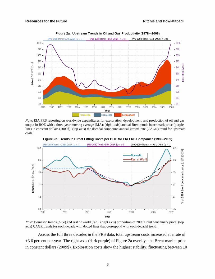
Figure 2a. Upstream Trends in Oil and Gas Productivity (1978–-2008)

Note: EIA FRS reporting on worldwide expenditures for exploration, development, and production of oil and gas

output in BOE with a three-year moving average (MA); (right-axis) annual Brent crude benchmark price (purple

line) in constant dollars (2009$); (top-axis) the decadal compound annual growth rate (CAGR) trend for upstream

costs.

Figure 2b. Trends in Direct Lifting Costs per BOE for EIA FRS Companies (1980–2009)

Note: Domestic trends (blue) and rest of world (red); (right axis) proportion of 2009 Brent benchmark price; (top

axis) CAGR trends for each decade with dotted lines that correspond with each decadal trend.

Across the full three decades in the FRS data, total upstream costs increased at a rate of

+3.6 percent per year. The right-axis (dark purple) of Figure 2a overlays the Brent market price

in constant dollars (2009$). Exploration costs show the highest stability, fluctuating between 10


7

and 30 percent of Brent crude. Production costs dominate throughout the early portion of the

time series (1978–1996) until development expenditures become the highest proportion of

upstream spending from 1997 onward. Notably, the three-year moving average of upstream FRS

expenditures exceed the Brent market price for much of the period during 1997–2002—signaling

market prices that reached unsustainable levels for the industry in the long term. The increasing

dominance of development costs in the late 1990s indicates a growth trend in industry capital

expenditures, contributing to the supply-side conditions for the following decade’s oil bull

market.5

Industry trends for production, development, and exploration costs reported in the FRS

(Figure 2a) align with the initial formulation of the LBE model in the period leading up to its

original publication. From 1988–1996, total upstream costs per BOE of oil and gas output

experienced an average -1.1 percent annual cost decline (𝜌 +1 percent). Though these

productivity gains did not translate to subsequent decades, this portion of the time series shows

gradual improvements in oil and gas production costs as a learning effect one would expect for a

homogenous product.

The closest equivalence between the cost ranges reported in the H-H-R supply curve and

industry metrics are reported direct lifting costs. 6 Lifting costs account for the expenditures

required to extract developed reserves after they are found and acquired. EIA FRS data on direct

lifting costs provided in Figure 2b indicate that the technical cost of extracting oil and gas rose

+0.7 percent per year from 1980 to 2009.

The three decadal cost trends range from negligible (1980–1990), to a sharp compound

annual decline of -5.5 percent (1990–2000), and a rapid increase (+9.0 percent) in the first

decade of the twenty-first century. From 1980–1992 the trend indicates a -1.0 percent annual cost

decline from improving productivity. This sub-period appears to show the effect of learning from

continuous production with conventional technologies in well-characterized geographic regions,

5 The FRS data report aggregate oil and gas production, so these values are not directly indicative of actual producer

marginal cost, or useful for calculating profit margin. While providing an internally consistent data set for upstream

costs and production, the aggregation of oil and gas data makes disaggregation dependent on a series of complex

assumptions.

6 Though Rogner (1997) argues full upstream costs from exploration, development and production are captured in

this model because of evidence suggested by development in the United States and production in the North Sea, and

we contend that supply curves produced by the LBE approach more closely correspond to the direct lifting costs

associated with production (e.g. operational expenditures). This case is argued throughout the following Section 2.2.


8

shaping the initial formulation of the LBE concept, which anticipates that these productivity

gains would extend and continue for all geologic oil and gas resources.

Although the EIA is only one source for data on industry productivity, these upstream

cost trends mirror the general features of other academic studies (Fantazzini, Höök, and

Angelantoni 2011; Mitchell and Mitchell 2014); financial institution publications (Syme et al.

2013; Deloitte 2015; Goldman Sachs 2014, 2013; JP Morgan Asset Management 2015; Lewis

2014); and reports from oil industry consulting agencies (e.g., Kopits 2014; Rystad Energy

2015). We have elected to focus on the EIA FRS data because it is the highest quality dataset we

could find in the public domain and available to readers for additional scrutiny. Additional

efforts can harmonize these data with upstream trends from the most recent decade. Admittedly,

while including worldwide measures for Canada, Europe, the former Soviet Union, Africa, the

Middle East, and other parts of the world, these data are biased toward US operations. Therefore,

an immediate question arises about the application of these upstream trends to studies of global

oil and gas supplies, where OPEC producers play a major role.

We agree with Watkins (2006) that the deregulation of US oil prices in 1981 plugged the

domestic market into the world, allowing information from the United States to provide a

window into reserve prices and costs in all regions open to new investment. As non-US

companies develop and explore for oil in the United States with operations around the world, the

EIA FRS data series can be considered to generally represent the “shape” of costs in many parts

of the world. Global price trends have mirrored these upstream costs, suggesting they are

generally representative of industry marginal cost and performance trends.7

The LBE theory expected that compounding gains in performance would lead to ongoing

cost declines from accumulated learning. Yet total upstream costs indicate an extended period of

aggregate performance declines for total global oil supply. Despite specific performance

increases in some regions and the rapid diffusion and innovation in new upstream technologies

(e.g., especially horizontal drilling post-2005), sustained periods of productivity trends from

1978–2009 break from LBE projections. This discontinuity indicates that a model of autonomous

non-price–induced learning for conventional oil and gas supply technologies does not capture

relevant characteristics of the frontier between production technologies of the past and those of

7 Operations in the United States are less subject to political instability than in many regions; however, they may be

more expensive due to concerns about litigation and social license.


9

the future. A continuous learning effect applied to a heterogeneous resource base will thus face

essential constraints in modeling the productivity of new technologies needed to access different

types of resources in varied geologic formations.

The analysis in this section leads us to propose that specific manufacturing processes for

future oil and gas production must be considered in models of long-run technological change to

resolve contradictions between empirical trends and theoretical expectations for contributions

from learning. The importance of introducing higher resolution modeling for extraction

technologies is further illustrated by the context of capital expenditures.

2.2. Market Prices and Measured Productivity: Distinct Patterns for Operational and Capital Expenditures

The LBE theory expects that a learning effect independent of market price is a suitable

explanation for productivity improvements in upstream energy resource extraction costs.

However upstream costs are also contingent on a range of non-technical factors, including taxes

and royalties, land valuations, political intentions and business cycles.

Osmundsen and Roll (2016) explore evidence of industry cycles on upstream

expenditures and provide evidence that bullish periods lead to increases in costs per unit of

output, reducing measured productivity. In periods of rapid expansion, oil rigs and other oilfield

service equipment experience a faster hike in wages and rig prices, which reduces measured

productivity, due to pressure from higher rates of capacity utilization. Conversely, in a market

slump, equipment utilization rates decline, rig rates fall, and upstream productivity measures

increase.

The FRS upstream costs we analyze mirror patterns in market price, but are these

fluctuations in productivity more clearly shaped by demand- or supply-driven gains from

learning? Rogner (1997) equates long-term price in LBE supply curves to marginal costs (P =

MC) determined by technology that improves with learning to formulate cost projections

dominated by supply-side factors. If learning-by-doing dominates upstream costs, an

autonomous stable productivity trend is an appropriate model, since the costs of investing in

supply expansion are largely independent of demand. However, Osmundsen and Roll point to

one important way that demand-led prices shape marginal cost profiles, suggesting that point

estimates of upstream productivity independent of market conditions may not be applicable.

While the EIA FRS data do not have enough resolution to develop a test of causality

between market price and upstream productivity with robust econometric analysis, we broadly


10

examine these relationships in Figure 3a-b. Production costs are summarized as operational

expenditures (opex) and development plus exploration costs as capital expenditures (capex).

Figure 3a plots the year-to-year change in Brent price (top) alongside measured

productivity gains for opex (middle) and capex (lower) from the FRS data in Section 2.1. Price

declines visibly precede productivity gains through the early 1980s, suggesting much of the

“learning effect” measurable over this period resulted from industry consolidation. Parallel

productivity gains in this series for opex are far less volatile than capex, and consistent with what

a learning model would expect: 1991–1999 shows an eight-year stable improvement in

operational productivity (𝜌 ~ +3 percent). Because long-term models smooth trends to maintain

numerical tractability, the histograms (right-side) highlight empirically consistent normal

distribution fits with mean values over the entire time series for opex of 𝜌 = -4 percent (dashed

yellow line) and 𝜌 = -5 percent for capex (dashed orange line).

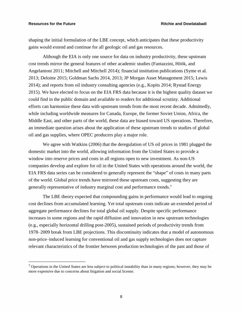
To test for the relevance of price effects, Figure 3b shows the influence of market

fluctuations with year-to-year marginal changes in productivity measured per dollar of market

price (𝑑𝜌

𝑑$). Once again, the theoretical framework of LBE shows close correspondence to opex

trends: production expenditures experience little sensitivity to market price throughout the time-

series, as Rogner (1997) originally assumes for total hydrocarbon energy supply.

A simple time series average for opex indicates the productivity of operational

expenditures fell by 0.08 percent for every dollar increase in market price (𝑑𝜌

𝑑$= -0.08), but an

equilibrium value is close to zero. We interpret this as further confirming the validity of a non-

price–induced productivity model for opex. However, this assumption does not extend to capital

expenditures where marginal productivity rates fluctuate significantly from 1979–2008.

The overall relationship between price and capex in this time-series is broadly negative

(𝑑𝜌

𝑑$< 0), suggesting the industry tends to commit capital investments when market prices

increase. The cyclical nature of this trend indicates the industry adjusts expenditures based on

what the market outlook allows over any multi-year period. Large positive values for capex in

1990, 1997, and 2003 may indicate points where the industry was temporarily starved for capital

from underinvestment over the preceding period, and it is playing catch-up. Significant increases

in amplitude during the latter half of the series may account for the scale-up of capital

investments needed to extend production into areas that required deepwater drilling and

hydraulic fracturing, alongside boom times for the industry in the early twenty-first century.


11

Figure 3. Relationships between Upstream Spending, Measured Productivity Changes and Market Price (1978–2008) for EIA FRS companies (3-yr MA)

Figure 3a. Market Price and Upstream Productivity Trends Multi-Plot

Notes: 1978–2008 time-series (left column) and histogram with normal distribution fit (right column) for 3-yr MA

change in Brent market price (purple line, upper); measured productivity improvement for operational expenditures

(yellow line, middle); and capital expenditures (orange line, lower). The original Rogner (1997) estimation of 1%

annual productivity gain is overlaid on the time series (dark blue dotted line, upper) along with the average

productivity improvement for opex (dashed yellow line, middle) and capex (dashed orange line, lower); each plot

includes gray lines for the other two data series out of focus.


12

Figure 3b. Marginal Upstream Productivity Rate per Dollar of Change in Market Price - (𝒅𝝆

𝒅$) for Operational

Expenditures (yellow line) and Capital Expenditures (orange line)

Since many oil and gas companies employ significant teams for forecasting and strategy,

decisions to commit development costs are undoubtedly contingent on scenarios for market

outlooks. This analysis suggests the relevance of simulating market conditions for projections of

upstream productivity over the long run. It seems difficult to harmonize an outlook for optimal

investments that result in supply-led marginal costs determined by a 1 percent per year learning

improvement with an industry that undertakes marginal capital investments under an expectation

of higher market prices.

As visible in the FRS data from 1998–2008, development expenditures continue to

accelerate in line with market prices (Figure 2a and 3a), indicating that the projects expanding

marginal supply from the expensive end of the cost curve receive a green light under outlooks for

continually increasing prices. If a 1 percent per year improvement in total upstream productivity

had occurred from 1988–2008, total upstream costs would have fallen from $24.50 per barrel to

$20 per barrel by 2008, and expenditures on capex would have declined from $13 to $11 per

barrel. Such a projection would have underestimated total upstream costs over these two decades

by an average of 60 percent per year and capex by 100 percent per year. In this case, the LBE


13

theory would have anticipated an equilibrium Brent market price of $26 per barrel through the

period from 2000–2008 over which Brent market prices averaged $60.8

Overall, it is unlikely that year-to-year average productivity measures for capital would

maintain such distinct volatility across the industry. We therefore interpret these fluctuations of

measured annual productivity in capex as indicating the dominance of essential business cycle

elements over a measurable level of pure endogenous learning in this time series. These are the

factors originally discussed by Schumpeter (1934; 1939): during an upturn, wages increase and

labour productivity decreases; during downturns, the opposite occurs, as companies throttle

expenditures for production capacity based on market outlooks. 9

FRS data illustrate important and relevant macro-scale aspects of the trends explored at

the micro level by Osmundsen and Roll (2016): short- and medium-run constraints on production

equipment during booms drive up costs because limited supplies of oil-field capital and labor

may command higher prices. Accounting for such demand-led marginal costs in a long-run

supply model is necessary: socioeconomic conditions of many long-run policy models are

predicated on a “long boom” of equilibrium growth in economic output (Clarke et al. 2014).

Total upstream costs per unit of production decline in a market bust, but resulting

productivity measures are dominated by the expenditure reductions driven by responses to

market conditions—and not the influence of learning. Capex productivity improvements in these

data under such an economic environment seem to primarily reflect curtailed expansion of

production to new areas. Even though market pressures drive innovation, aggregate industry

productivity data require a careful analysis that accounts for explicit technological improvements

alongside potential bear or bull market conditions—an insight particularly relevant for oil, gas,

and coal production data collected during the commodity bear market that started in 2014.

While short, multi-year downturns merely constrain future output growth, extended

periods of low capital investment will eventually lead to maturing production and well depletion,

8 This projection of market prices maintains average mark-up per barrel in the FRS series of 30%.

9 These measures are further complicated because of the long-run outlooks required to develop new fields, i.e.

market price outlooks for development expenditures must look beyond 3-year moving averages. However, this

comparison is developed with 3-year MA market prices to make a one-to-one comparison with the original FRS

data. In many regards, a year-to-year measure of capex productivity is limited but this is provided to match the

annual point estimates in the LBE model.


14

a 9 percent annual decline that sustained investment tends to reduce by 3 percent in aggregate.10

Measured productivity gains due to a period of oversupply and falling oil prices do not

inherently translate to increased long-run output potential because the production of oil resources

are inherently different from manufacturing of an homogenous product: the production profile of

specific wells and fields declines over time.

This analysis of FRS data indicates that: (i) the LBE model accurately captures non-

price–induced secular trends for spending on operations; and (ii) the performance of energy-

sector capex is poorly represented in a homogenous formulation of marginal costs driven by the

accumulation of learning.

Accordingly, some element of observable market price effects must inform a model of

long-term industry productivity trends to overcome biases introduced by aggregating operational

and capital investment dynamics in the LBE theoretical approach to upstream cost. Plausible

simulations of long-run oil and gas supply costs require an explicit representation of the industry

decision context for capital expenditures.

2.3. How Relevant Is an Equilibrium Reserve-to-Production Range for Calibrating Future Upstream Cost Profiles?

The LBE theory draws from a reserve-to-production (R-P) ratio for oil and gas, which

maintained relative consistency over the twentieth century, suggesting that recoverable reserves

can be conceptualized as a flow that continually draws from the total stock of geologic resources.

Therefore, resources are continually reclassified as reserves with production at costs subject to

productivity improvements driven by learning. This is the underlying concept for an equilibrium

R-P ratio—it is maintained within a consistent range of values by ongoing development of

resources into reserves. The equilibrium R-P ratio intends to represent the behavioral dynamic of

producers who otherwise have little incentive to invest in knowledge of energy resources at

lower production rates. However, the last few decades of data challenge the relevance of this

assumption to projections of upstream costs driven by learning and the accumulation of

knowledge.

10 The IEA World Energy Outlook 2016 highlights that depletion rates for global mature fields are around 9%, but

sustained investment reduces decline of producing fields to 6% (IEA, 2016). Fustler et al. (2016) review the

academic literature on decline rates, estimating a 6.2% per annum rate post-peak.


15

Even as R-P ratios for oil and gas can remain relatively stable, the expenditures necessary

to develop reserves into production have varied. A growing reserve base doesn’t inherently

ensure that oil is getting cheaper to produce, and can often mean the opposite. The costs of

converting proven reserves into a producing well are accounted as development expenditures. In

the LBE theoretical approach, development expenditures represent the costs of moving the

dynamic boundary that differentiates the total geologic stock of an energy resource from its

reserves, and their eventual production. Figure 4a-c plots several relationships between

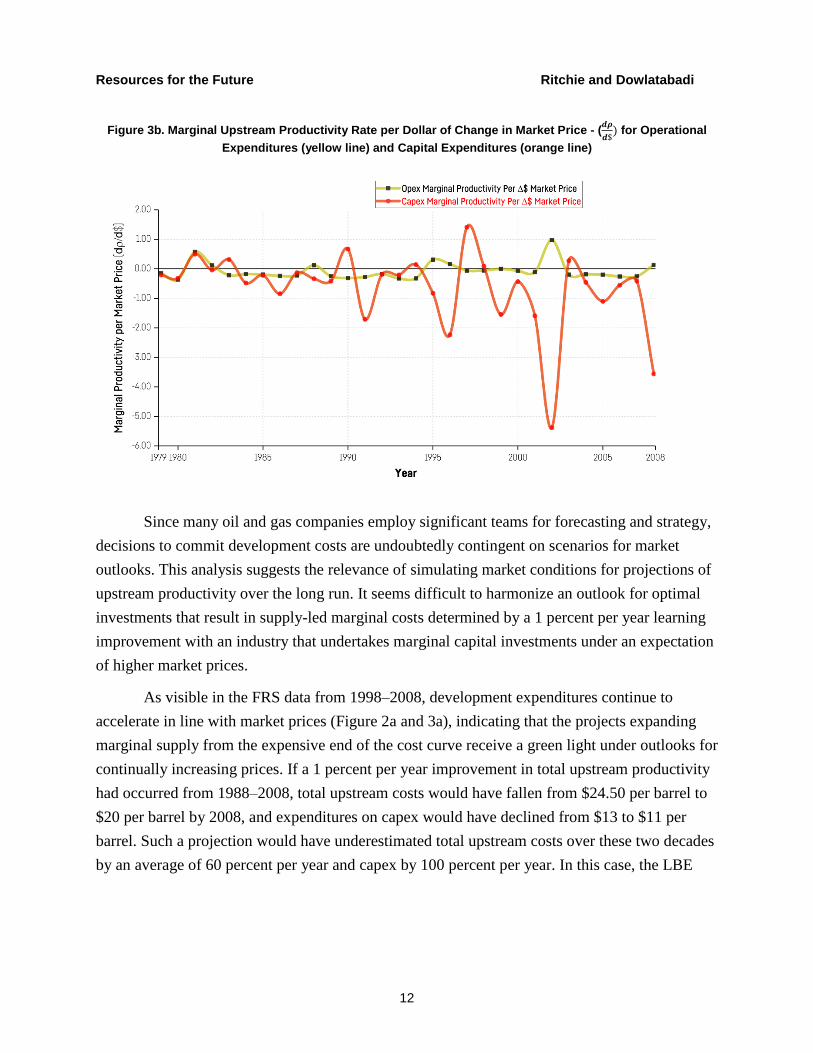
production, reserves, and development costs for oil and gas. Figure 4a depicts the proportion of

exploration, production, and development costs in the EIA FRS. Development as a fraction of

upstream costs remained relatively stable from 1978–1991 but grew steadily from 1992–2005.

Data from EIA FRS companies indicate that total expenditures on development grew from $7.50

per BOE in the mid-1990s to $36.50 per BOE in the mid-2000s. Over this period, development

costs grew 4.8 percent per year from 1978–2008, outpacing growth in operating costs by 56

percent.

As an aspect of total industry marginal cost, development costs will be reflected in

market price. Over the last few decades, development costs have mirrored trends in market prices

much closer than trends in exploration or production costs (see Section 2.2). We suggest that by

focusing on the technical operating costs of producing wells, the LBE supply curves applied thus

far in the literature reflect only one-third of the marginal cost of oil and gas production. This has

neglected the cost and performance dynamics of the boundary between resources, reserves, and

production—especially as significant unconventional resources were being developed.

Development costs are highly sensitive to aspects of technical difficulty introduced by geology

or geography.

Adelman (1995) characterizes essential features of industry behavior with a warehouse

metaphor, where reserves are the dynamic inventory. This warehouse inventory is replenished

from the resource base and depleted through production, with reserves established by

expenditures on development. Adelman highlights that production capacity is likely to increase if

development costs are below the equilibrium market price, but intensive periods of development

raise the marginal cost per barrel of output, continually testing the equilibrium value. This

interplay between supply and demand converts the marginal warehouse inventory of reserves

into production as fast as the equilibrium market can rise.

Accordingly, we suggest that the relationship between expenditures on reserve

development and demand drives cycles of marginal cost and market price that fluctuate around


16

the base of proved reserves. An autonomous equilibrium R-P ratio provides little information on

the availability of long-run supply if applied independently of development cost trends. 11

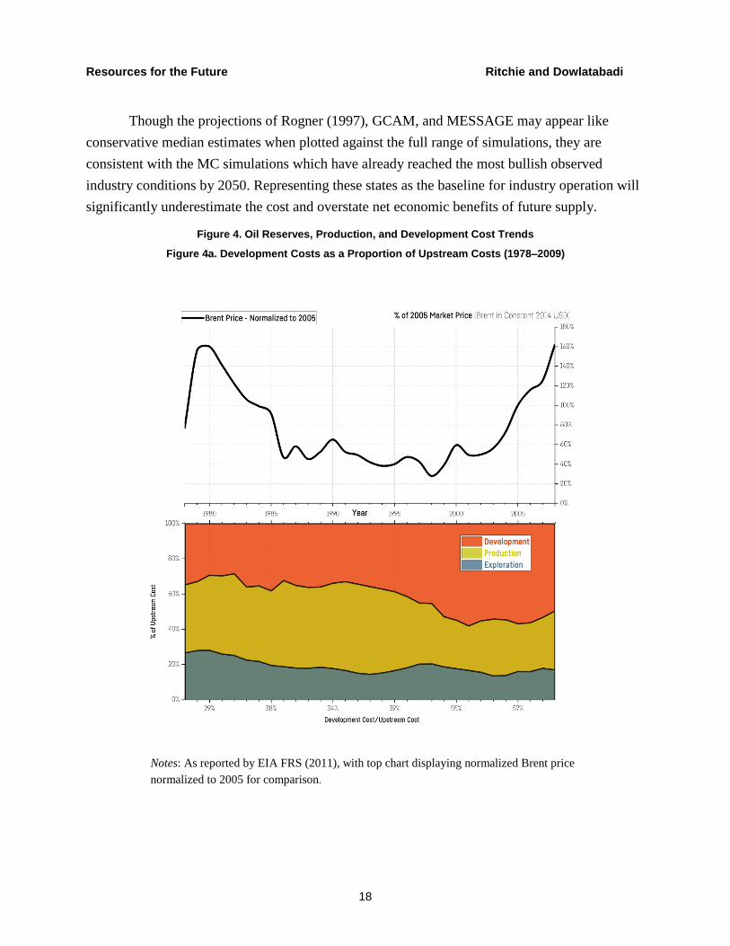
A stylized version of these cycles is illustrated by a ratio of proven reserves and market

prices (R-to-Price).12 When plotted (Figure 4b), industry data suggest the realization of reserves

has fluctuated through two major cycles between 1955 and 2015. Each point on the curve in

Figure 4b represents the size of the global oil reserve warehouse and the cost of converting it into

production. A lower value indicates fewer reserves or higher costs (more expensive warehouse

withdrawals) and vice-versa. In this series, peaks in the ratio of proven reserves-to-price occur in

1970 and approximately 1997–2001; troughs occur in the mid-1950s, 1980, and perhaps 2016.13

In this cycle, increasing overall costs test the maximum threshold of market demand.

Once market equilibrium no longer supports further growth in development costs, pressure eases

on the need to sustain high production growth rates. At this point, upstream costs consolidate

around ongoing viable operating production at a lower market price level (the 1980s and 2014–

2016). Regardless of the exact mechanism generating these two cycles, they indicate that the

industry conditions that lead to increasing reserves at lower cost only characterize one-half of

each cycle since 1955. The presence of reserve base cycles suggest the initial formulation of the

LBE theory is based on a convention that projects dynamics consistent with the upward swing

(1980–2000).14

Though the LBE supply model as applied in Rogner (1997) and subsequent studies

allows the total size of the warehouse to grow, development costs that would govern the rate and

costs of “warehouse withdrawals” are noticeably missing—such as Adelman’s (1995)

11 The snapshot of a reserve base at a point in time will include a portfolio of projects with a range of necessary

development costs to realize production consistent with today’s output. The view of Adelman (1995) is that the

stock of geologic oil resources is irrelevant, and what matters is the development cost needed to provide a regular

flow of oil production. 12 Market prices are assumed to reflect some aspect of medium-run marginal costs related to mobilizing reserves—

i.e., reserves anticipated to be economically viable are developed at expected market prices. 13 Data for oil prices and reserves were collected from the BP Statistical Review (2015) and for 1948-1980 from the

Oil Economists’ Handbook (Jenkins, 2005). 14 One possible interpretation of these cycles could build from structural adoption of present and future oil demand

that generates alternating states of pressure and release on the reserve base. As the reserves in the present become

cheaper (upward ascent of each cycle), development costs accelerate to keep production capacity growing on pace

with the demand that readily results from increased availability. As the rate of adoption increased from the 1990s

through the early 2000s, development costs increased as a proportion of upstream spend (Figure 4a).


17

observation that development costs increase rapidly during periods of high capacity use.

Therefore, we argue that the LBE conceptualization of dynamic oil and gas resources focuses on

inputs to the reserve warehouse but poorly captures aspects of realizing the warehouse

inventory’s potential for production.

Because development costs are an important element of marginal production cost largely

missing from long-term supply curves shaped by the LBE theory, the resource-to-reserve-to-

production dynamic applied to future oil, gas, and coal are only consistent with an outlook for

permanently optimal investment, where supply is expanded at the lowest possible cost in perfect

foresight. Costs of oil and gas supply estimated by the LBE model are unmoderated by the

development costs and market prices that could diminish reserve growth, lower demand, or

decrease production in a competitive marketplace with a diversity of energy supply strategies.

The projection of a learning effect point-estimate from any single state in this reserve-

price cycle will result in an overabundant or overly scarce depiction of oil and gas supply. Each

point in the historic time-series of Figure 4b is a valid representation of the supply-demand

balance for the reserve base at a snapshot in time. Projecting a learning trend that smooths this

cycle by starting with a selected baseline period is likely to considerably miscalculate the cost of

mobilizing reserves in all future periods by establishing overly bearish or bullish conditions from

the outset.

To illustrate how this distortion is likely to occur, we conduct a Monte Carlo (MC)

simulation with 200 runs that randomly select a base year R-$ value (1950-2014) from a uniform

distribution of the underlying data from Figure 4b for calculation of compounded learning across

the twenty-first century. Projections of this reserve-to-price ratio are overlaid on Figure 4c for

600 gigatons of oil equivalent (Gtoe) (>140 years of supply at 2014 levels) from Rogner (1997),

GCAM (Joint Global Change Research Institute 2016) and 570 Gtoe from MESSAGE (Riahi et

al. 2012). Historical trends across a five-year moving average for proved reserves (P1) to

constant 2014 US$ (R/$) are illustrated by the solid black line which reproduces Figure 4b.

The mean year-2100 value from the results of our MC simulation is R-to-$ = 70.43,

which represents a steady-state reserve-base condition 55 percent higher than data indicate the

industry has ever experienced. By midcentury, the average value of all runs has surpassed

previous peaks in the late-1990s and early-1970s.


18

Though the projections of Rogner (1997), GCAM, and MESSAGE may appear like

conservative median estimates when plotted against the full range of simulations, they are

consistent with the MC simulations which have already reached the most bullish observed

industry conditions by 2050. Representing these states as the baseline for industry operation will

significantly underestimate the cost and overstate net economic benefits of future supply.

Figure 4. Oil Reserves, Production, and Development Cost Trends

Figure 4a. Development Costs as a Proportion of Upstream Costs (1978–2009)

Notes: As reported by EIA FRS (2011), with top chart displaying normalized Brent price

normalized to 2005 for comparison.


19

Figure 4b. Two Distinct Cycles in Reserves: Quantity of Proved Reserves-to-Brent Prices for Oil (1955–2015)

Notes: Right-axis indicates regions of each cycle which lead to increasing pressure on development costs and declining pressure on development costs; top-axis notes duration of cycle states from trough-to-peak and peak-to-trough.

Figure 4c. Range of Estimates from Relative Ratio of Proven Reserves to Price for Oil

Notes: Historic trend with 5-year moving average (solid black); a Monte Carlo simulation of 200 runs randomly selects from a base year R-$ value between 1950–2014 with uniform distribution and projects this value at ρ = 1% per year (thin lines); values for 600 Gtoe of oil (>140 years of supply at 2014 levels) are provided for Rogner (1997) and GCAM (2012) and 570 Gtoe for MESSAGE (Riahi et al., 2012)


20

As these cycles indicate, the relationship between reserves and price is more dynamic

than a monotonic decline in upstream costs and stable replenishment of reserves. When the

original LBE model was published in 1997, data from the preceding period would have

undoubtedly been influenced by the upward swing of the reserve-price cycle of 1980–2000. A

sustained negative slope in this reserves-to-price ratio is likely to create perception of increasing

scarcity, while a sustained positive slope could lead to a perception of increasing abundance.

Future research on long-term energy resources must strike a balance that recognizes the

cyclical nature of industry operations that moderate bullish and bearish periods. The boundary

between producing reserves and resources can move in directions that allow production of more

reserves at lower cost, and vice-versa.

Similar equilibrium R-P trends in conventional oil and gas are applied by the LBE theory

to characterize the total occurrences of geologic coal. We now examine the validity of a learning-

by-doing model with a dynamic reserve boundary for the coal resource base.

3. Assessing the Learning Hypothesis for Total Geologic Coal Occurrences

Despite varied development costs for recovery of oil and gas, increasing knowledge has

generally led to the discovery and classification of more reserves over time (e.g., Adelman and

Watkins 2008; Watkins 2006). LBE supply curves hypothesize that the resource-to-reserve

dynamics of oil and gas can characterize the future of the coal resource base. While increasing

knowledge of oil and gas has discovered more economically recoverable reserves, coal resources

have followed the opposite pattern (Ritchie and Dowlatabadi 2017).

As coal deposits are generally easier to discover and assess than oil and gas, coal

availability studies often start by establishing the largest possible quantity of total coal resources

(Fettweis 1976; Höök et al. 2010; Rutledge 2011). After an initial assessment determines the

amount of coal in a deposit, a process of ongoing subtraction clarifies the portion recoverable as

reserves (e.g., accounting for those that are too deep or for which the seam is too thin). An

economic assessment further shrinks the reserve base by eliminating portions of a deposit that

are not viable for profitable production. Several dimensions of hard coal resource assessments

relevant to an evaluation of the LBE theory are provided in Figure 5.

The process used by the US Geological Survey (USGS) to assess the coal resource base

(Figure 5a) demonstrates how increasing knowledge continually subtracts from initial coal

availability studies (Luppens et al. 2009). The original availability studies at the root of this


21

process are rarely updated. Recent documents from the USGS and the EIA still cite Averitt

(1975) as establishing primary data on the national coal resource base in many areas.

Recoverability studies are updated with more regularity, but tend to focus on specific regions

where coal mining is already ongoing (such as for the United States with Luppens 2009 and

Ruppert et al. 2002).15

The 1913 International Congress of Geologists (IGC) in Toronto established an original

aggregate assessment for global coal resources. Since then, the World Energy Council (WEC),

previously the World Power Council (WPC), and the German Federal Institute for Geosciences

and Natural Resources (Bundesanstalt für Geowissenschaften und Rohstoffe, BGR) have

maintained regular publications on global coal reserves and resources. As vintage editions of

these assessments can be difficult to procure, we rely on the twentieth-century values of the IGC,

WPC, WEC, and BGR reported by Fettweis (1976), Rogner (1997), Gregory and Rogner (1998),

Höok (2010), and Rutledge (2011).

These data indicate global coal reserve base trends have mirrored the USGS process of

ongoing subtraction. In other words, more of what used to be considered recoverable reserves

has been reclassified as resources over time, or simply removed from the records. Recent WEC

and BGR data are consistent with these trends.

The global reserves-to-resources dynamic for coal is depicted in Figure 5b, which plots

the Rogner (1997) synthesis of BGR (1989) and WEC (1992) next to recent BGR studies (BGR

2014, 2010) used by the IEA (2006–2015) and against Rogner (2012). To maintain consistency

with the H-H-R supply curve, energy units (Gtoe) for each coal assessment (Figure 5b) are

harmonized with physical units (gigatons) based on values used by Rogner (1997).16

An empirical learning curve for increasing knowledge about the global coal resource base

measures a -4.5 percent annual decline in reserves from Rogner (1997) to the BGR (2014)

assessment. A similar trend is present in the WEC and BGR vintage reserve data reported by

15 Initial availability figures for several nations come from assessments in the late 19

th-century, such as the initial

figure for China of 1,000 Gt provided by German geographer von Richthofen during his surveys from 1877-1911

(Fettweis 1976). Recent data available from the UK indicate that coal supply figures are consistent with those from

the 1870s (Department for Business, Energy, & Industrial Strategy 2015). Rutledge (2011) writes that in the UK, the

1871 Royal Commission provided the reserve estimate until 1968, after which the updated quantities of reserves fell

rapidly.

16 To ensure internally consistent comparisons, we follow the methodology of Rogner (1997) by using average

primary energy content values of each region.


22

Höok (2010), which includes lignite. Consequently, the global coal R-P ratio of more than 200

years (1980–2000) has fallen to approximately 100 years (2014).

However, any trend is difficult to ascertain because inconsistencies in data over time

make useful comparisons of dubious quality. Fettweis (1976) argues that the primary changes in

total world coal resources reported to the IGC (1913) and subsequent assessments through 1970s

were: (i) changes in reporting definitions on the depth limit of resources (up to 1,200m, 1,800m,

or no limit); (ii) the addition or subtraction of hypothetical “prognostic resources;” and (iii) the

correction of errors. These factors still appear to contribute to the notorious reputation of modern

global coal data.

IEA coal database figures on domestic coal supply do not consistently match reserve or

resource numbers in annual Coal Information reports (IEA 2015). Despite growing production,

China’s reported coal reserves remained relatively static since 1992—confusion has resulted

from definitions of economically viable reserves and coal classified as basic reserves (Wang,

Davidsson, and Höök 2013).

Heterogeneous national definitions of reserves and resources further muddle varied

assessment techniques that blur the line between whether a nation’s coal reserves have been

quantified with a focus on economic or geologic factors (Fettweis 1979; Wang et al. 2013) or

whether a recovery rate has been applied in determining “recoverability” (BGR 2015). In recent

years, WEC has omitted reporting on global coal resources, focusing only on reserves.

More consistent reporting standards and definitions applied in the early twenty-first

century have increased overall knowledge of the global coal resource base. The learning that has

accumulated over this period about geologic coal has decreased the assessed quantity of reserves

(CIM 2014; Hartnady 2010; JORC 2012; Wellmer 2008). Despite upward revisions to reserves

in some regions over this period, cumulative production figures indicate that at least 20 percent

of the aggregate decline has resulted from factors attributable to learning: increasing knowledge

and improved reporting (Ritchie and Dowlatabadi 2017).


23

Figure 5. Assessing the Global Coal Resource Base over Time

Fig. 5a Process for Calculating Economically Recoverable Coal

Source: Adapted from USGS (2009)

Figure 5b. Coal Reserves as a Fraction of Recent Coal Resource Assessments

Sources: BGR 2014, 2010; Rogner et al. 2012; Rogner 1997.


24

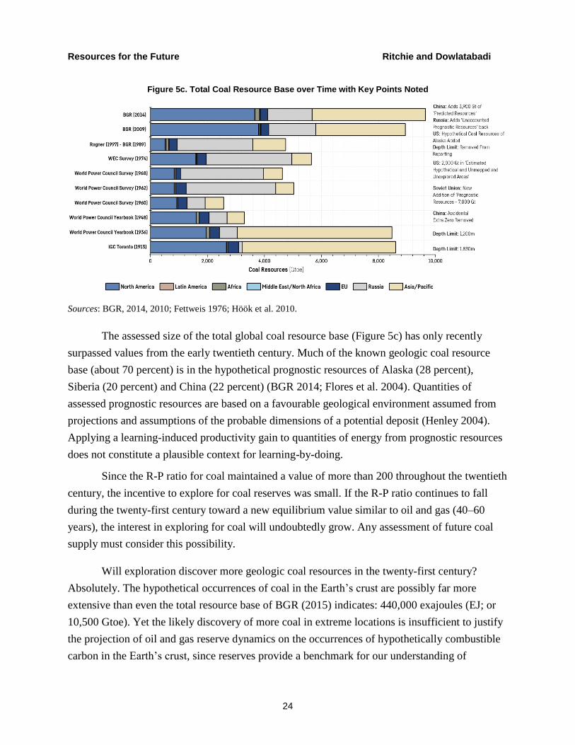
Figure 5c. Total Coal Resource Base over Time with Key Points Noted

Sources: BGR, 2014, 2010; Fettweis 1976; Höök et al. 2010.

The assessed size of the total global coal resource base (Figure 5c) has only recently

surpassed values from the early twentieth century. Much of the known geologic coal resource

base (about 70 percent) is in the hypothetical prognostic resources of Alaska (28 percent),

Siberia (20 percent) and China (22 percent) (BGR 2014; Flores et al. 2004). Quantities of

assessed prognostic resources are based on a favourable geological environment assumed from

projections and assumptions of the probable dimensions of a potential deposit (Henley 2004).

Applying a learning-induced productivity gain to quantities of energy from prognostic resources

does not constitute a plausible context for learning-by-doing.

Since the R-P ratio for coal maintained a value of more than 200 throughout the twentieth

century, the incentive to explore for coal reserves was small. If the R-P ratio continues to fall

during the twenty-first century toward a new equilibrium value similar to oil and gas (40–60

years), the interest in exploring for coal will undoubtedly grow. Any assessment of future coal

supply must consider this possibility.

Will exploration discover more geologic coal resources in the twenty-first century?

Absolutely. The hypothetical occurrences of coal in the Earth’s crust are possibly far more

extensive than even the total resource base of BGR (2015) indicates: 440,000 exajoules (EJ; or

10,500 Gtoe). Yet the likely discovery of more coal in extreme locations is insufficient to justify

the projection of oil and gas reserve dynamics on the occurrences of hypothetically combustible

carbon in the Earth’s crust, since reserves provide a benchmark for our understanding of


25

recoverable coal. Sustained declines in the coal R-P ratio over the last decade has not followed

the trend of oil and gas, where increased consumption has also increased reserves.

The economic and market conditions that may allow reserves downgraded since Rogner

(1997) to be reclassified as recoverable would also face stringent competition from a range of

other options of energy supply and demand. There are further issues with procuring enough

water, establishing social license, and navigating the legislative constraints necessary to realize

ambitious coal supply figures. As Figure 5a illustrates, social and environmental factors play a

major role in subtracting from the total coal resource base.

Including the full extent of the coal resource base in a twenty-first century supply curve

requires normative choices for coal supplies and technology, such as those Rogner (1997)

describes: drastic, specific progress in technology at a sustained rate several times the historically

observed average. This requires radical shifts from today’s coal mining technologies, outside the

scope of reasonable productivity improvements that could constitute plausible projections of a

learning rate or equilibrium reserve value.

Still, even if perfect data were available on cost trends of oil, gas, and coal production so

that aggregate productivity trends could be robustly interpreted, would it be possible to identify

and fully distinguish improvements attributable to learning?

4. Nordhaus (2009) on the Perils of the Learning Model: Applications to Energy Resources

The LBE theory for future hydrocarbon supply is conceptualized by Rogner (1997) with

market prices determined by marginal production costs over the long-run (P = MC). Market

prices are exogenous in this supply-led model, calibrated by the influence of endogenous

learning, which drives production costs with the cumulative experience that results from

continued extraction of the geologic resource base.

Though markets for energy commodities are global in scale, resources are locally

produced under myriad conditions dictated by firm structure, international politics, royalty and

tax accounting, technology, geology, and access to markets. Surmising an aggregate estimate of


26

macro-level productivity improvements is at best a speculative venture, as demonstrated by the

volatile year-to-year productivity rates described in Section 2.2.17

Nordhaus (2009) argues policy models that apply a learning curve to assess future

technological change for energy supply strategies are potentially dangerous: they are highly

sensitive to artificial learning rates that could be indistinguishable from measurement errors and

normative choices. He develops a theoretical case for a generic industry to illustrate that

productivity gains explained as “learning-by-doing” will always lead to upwardly biased

estimates of long-run productivity, because the influence of pure endogenous learning is difficult

to isolate and identify. His general theoretical case is summarized in the Appendix.

From this generic industry, Nordhaus suggests that: (a) there is a fundamental statistical

identification problem in separating an endogenous learning effect from exogenous productivity

gains; (b) the subsequent estimated learning coefficient is generally biased upwards; (c) model

parameters intended to represent learning effects are not robust to alternative explanations and

specifications; (d) overestimates of learning coefficients will underestimate the total marginal

cost of output for a technology; and (e) optimization models that rely on learning curves are

likely to simply choose technologies that incorrectly or arbitrarily specify a high learning

coefficients (e.g., an upwardly biased long-run learning rate for any technology will allow it to

“rise above the rest”).

Though Nordhaus (2009) agrees that productivity benefits follow as workers in firms

gain experience with a production process, he expresses skepticism that embodied learning can

be measured reliably for large global systems. The “supply” of accumulated learning could be

embodied in a firm, a group of workers, an individual worker, or it could result from

international or interindustry spillovers. Further, a measured learning improvement may not be

durable.

The case developed by Nordhaus (2009) for exaggerated learning in a generic industry

(see Appendix) can be adapted to examine the theory of LBE by considering specific technical

features of oil and gas extraction.

17 We agree with Rogner (1997, 250): “Because data are consistently poor and have limited availability, estimating

productivity gains over extended periods of time is a risky undertaking. Hence, there could be a wide margin for

error around this productivity estimate. The projection of a long-term 1% per year growth rate may well prove too

conservative (or too optimistic).”


27

4.1. Drilling into Factors of Oil and Gas Productivity: More than Learning-by-Doing

Hamilton (2012) analyzes the impact of technology and price on oil production over the

last century in the United States (1859–2010) and across the world (1973–2010), extending far

beyond the small window covered by EIA FRS data in Section 2 of this paper. Hamilton draws

on these data to conclude that individual oil-producing regions have not demonstrated a pattern

of continuously increasing productivity from ongoing technological progress.

In Hamilton’s view, price incentives and technology have reversed declines in output

resulting from geological or geographic factors, but only temporarily. Measured productivity

gains in oil-producing regions initially increase as new fields are developed, followed by

productivity declines dominated by the natural depletion rate of wells. Hamilton suggests that the

historical source of industry productivity gains and increasing global oil production during the

twentieth century has been the exploitation of new geographical areas.

While Hamilton is only focused on empirical aspects of the past and does not consider

the potential long-run theoretical contribution of learning and unspecified technological

breakthroughs to productivity, his analysis serves as a reminder of the engineering factors related

to geology and geography that distinguish the oil and gas industry from other forms of

manufacturing.18 The determination of a true learning rate for oil and gas could be further

distorted by such complex industry conditions, adding another element to the issues raised by

Nordhaus (2009). For energy resources, it is unclear whether the role of learning and upstream

technology improvements can always be fully distinguished from productivity gains resulting

from specific geographic or geologic factors.

This dilemma mirrors echoes Adelman (1990): that the oil industry is an “endless tug-of-

war between diminishing returns and increasing knowledge.” As currently formulated, the LBE

model projects future supply costs as determined by a function of increasing knowledge, which

pulls Adelman’s tug-of-war in a single direction.

18Further, given the important role of oil in the economy, wholly political decisions have resulted in rapid growth of

output and subsequent price declines (outside of what any would consider as free-market equilibrium conditions) at

the moment these political concerns are left aside, as well as oligopoly or monopoly features that could create price

declines to consolidate market share. The Nordhaus (2009) model could further extend to capture price declines

induced by cartel decisions.


28

The cycles of cost and reserves reviewed in Section 2 suggest that Adelman’s metaphor is

apt: the reserve base does get pulled in both directions. Though application of an LBE supply

curve generally uses lowest-cost resources first, this weakly captures the effect depletion may

have on costs of accessing the full geologic resource stock over the long run, and misses an

opportunity to understand the investments needed to offset declines.

The use of compounded learning as the prime determinant of projected future costs of oil

and gas supply develops Adelman’s industry metaphor in a way that confirms the concern of

Nordhaus (2009). Hamilton’s analysis highlights the factors of oil production that counter the

increasing returns from knowledge and learning, indicating a path toward integrating the insights

of Nordhaus and Adleman. Global oil and gas production in the twenty-first century will balance,

benefit, and suffer from both increasing knowledge and diminishing returns.

4.2. A Case of Measuring Learning-by-Extracting alongside Geological and Geographical Factors

Accordingly, the case of Nordhaus (2009) can include a factor relevant to productivity in

the oil and gas industry. We introduce 𝑜 to represent a parameter for upstream productivity that

results from geographic expansion and geological conditions. When the price, cost, output, and

growth assumptions of Nordhaus (2009; see Appendix) are adopted, the original equation for

declines in price (𝑝) as a function of productivity gains results as Equation 1.

𝑝 = ℎ + 𝑜 + 𝑟(𝜖 + 𝑧) (1)

In this equation, the rate of true endogenous learning is denoted by 𝑟, exogenous

technical change by ℎ, constant price elasticity by 𝜖, and 𝑧 is a function of autonomous, non-

price–induced growth.With this modification, the industry cost function is assumed to involve

factors specific to engineering for oil and gas extraction (𝑜), which may also influence

productivity independent of learning-induced technical change.

In a case that considers production from an oil well in Texas, 𝑟 would capture

endogenous learning that leads to productivity improvements for onsite extraction (e.g., the local

crew gets better at operating the well). The specific location and geologic nature of the oil well

would impose productivity considerations captured by 𝑜, such as favorable drilling conditions

resulting from the initial pressure at the wellhead or the natural profile of production increases

and declines indicative of a maturing oil well.

Following from Equation 1, a calculation of the learning coefficient 𝜌 for this case results

in Equation 2, where exogenous and true endogenous learning are combined with productivity


29

gains enabled by geology and geography. If we adopt the values of exogenous technical change,

used by Nordhaus (see Appendix), with a true learning rate of 𝑟 = 0.25 and consider that geology

or geography may contribute a 1 percent productivity gain (𝑜 = 0.01), then the learning

coefficient would be measured at 𝜌 = 0.5, twice the true rate of learning (𝑟).

𝜌 =𝑝

𝑔=

ℎ+𝑜+𝑟𝑧

𝑧+𝜖ℎ+𝜖𝑜=

0.01+0.01+.25×0.04

0.01+0.01+0.04= 0.5 (2)

With these plausible values for exogenous technical change, autonomous growth and

demand elasticity, the sensitivity of 𝜌 to 𝑜 and its relationship to 𝑟 can be further considered:

with 𝑜 → 2𝑟 the marginal contribution of 𝑜 to 𝜌 rapidly declines as the calculated learning curve

approaches unity. Following from this case, even if 𝑜 were twice the value of 𝑟, the calculated

effect would remain roughly unchanged from when 𝑜 < 0.8𝑟.

If we interpret the H-H-R (1997) assumption of 1 percent endogenous learning for global

oil and gas as 𝜌 = 0.01, using the structural form of Equation 2, we can isolate the relationship

between 𝑜 and 𝑟 in Equation 3, with a learning curve effect summarized by Ω = 0.2375

𝑟 , where

the negative slope indicates that 𝑜 and 𝑟 are inversely correlated. 19

𝑟

𝑜= −(24.75 + Ω) (3)

It follows from Equation 3 with the learning rate of +1 percent: (i) 𝑜 and 𝑟 are highly

sensitive to each other and could easily be conflated, or mask their relative contribution.

Furthermore, that (iia) the sustained high level of true learning is needed to compensate for a

slightly negative contribution by 𝑜; or, conversely, (iib) a high level of learning could appear low

with a slightly negative contribution from 𝑜.

In a case where geological conditions result in a negative contribution to productivity and

increasing prices, such that 𝑜 = -1.5 percent, then the equivalent learning rate to sustain a +1.0

percent productivity gain on average in Equation 3 would need to sustain 13 percent per year;

further a -2.0 percent contribution by 𝑜 would need a continual 25 percent true learning rate.

19 We simplify Equation 3 with Ω which describes a learning curve effect on geography and geology: a higher value

for 𝑟 reduces Ω and calculates a smaller negative slope for the relationship between learning productivity and

geological/geographical productivity. Though the elasticity of demand for Equation 3 is consistent with Nordhaus’s

example in this case (ϵ = 1), an updated value for long-run oil demand elasticity for oil of ϵ = −0.072

(International Monetary Fund 2011) yields only a slightly different equation of r+0.2402

o= −25.02 , which doesn’t

significantly change the relationship of the variables here.


30

Conversely, a high true learning rate of 25 percent could be misconstrued by this slightly

negative value of 𝑜, underestimating the influence of technological change.

In summary, a measurement of learning-induced productivity that fails to capture the

effect of 𝑜 could readily obtain a biased value for the effect of learning-by doing on oil and gas

production. These considerations illustrate that truly disentangling the contribution of

endogenous learning from geology, geography, or exogenous factors is extremely difficult

without explicit studies of producing fields. Establishing the appropriate value of a learning

parameter for long-term fossil energy supply is a complex process that needs a further robust

modeling effort to remain relevant in future studies on climate and energy policy.

For the FRS data considered in Section 2, the mean value for decadal upstream

productivity appears to be negative (𝜌 < 0), further complicating the picture. Was endogenous

learning negative or did geology, geography, or exogenous factors dominate cost increases?

Presuming a deterministic level of true learning over a long time frame needs to overcome

measurement issues such as these to become a plausible description of future hydrocarbon

economics. When an observable productivity trend is the product of two unknowns, guessing the

value of each without an empirically constrained distribution of plausible values is difficult to

separate from a normative choice.

4.3. Implications of Learning Effects for Long-Run Energy Economics and Climate Change Mitigation Cost Projections

Fossil energy supply curves constructed with the LBE theory generally indicate that the

vast quantity of fossil occurrences in the Earth’s crust will readily dominate twenty-first century

choices for energy supply. Policy goals for reducing carbon emissions to limit future climate

change thus face stringent competition from the low-cost hydrocarbon deposits expected to result

from compounded learning. The projected cost of any backstop technology that could readily

substitute for these resources can also receive a bias from any selected learning rate. We provide

a simple example to illustrate the sensitivity of future backstop and policy costs to a chosen

learning rate.

If annual oil production growth continues across the twenty-first century at 1.1 percent

per year (2000–2014 trend), 660 Gtoe is withdrawn from the H-H-R supply curve. Varied rates

of productivity from +1 to -1 percent applied to the oil cost ranges calculated by Rogner (1997)

(Figure 6) adjusts the total discounted cost of supply by more than a factor of 7. As this case for

oil demonstrates, a greenhouse gas emission reference scenario adopted as a mitigation policy


31

baseline that relies on an upwardly biased learning rate for twenty-first century fossil energy

supply can easily underestimate the cost of future oil supply by 1.6 to 7.4 times per barrel.

Understating the cost of oil supply will also overstate the investment required to mitigate

its greenhouse gas emissions with a low-carbon alternative. If we equate the cost of future oil

supply in the 𝜌 = + 1.0 percent case to an average market price of $50 per barrel over the

century, a $120 per barrel zero-carbon backstop oil substitute available today appears as a

significant cost: a 60 percent reduction in the backstop cost is required for substitution with no

deadweight loss. Yet with an oil supply calculated at 𝜌 = -1.0 percent, this backstop is already

200 percent more cost-effective than oil over the long run—optimal energy policy in this case

calculates that short-run substitution should be incentivized because of negligible deadweight

losses.20

Figure 6. Cumulative Discounted Cost of Twenty-First Century Oil Supply

Notes: Growth in oil production at a 2000–2014 consistent level (1.1% per year) with H-H-R price bands at learning

rates of 𝜌 = +1%, 0.5%, 0%, -0.5% and -1% for discount rate of 5%; right bar multiples of total twenty-first century

oil supply cost compared to the 𝜌 = +1% case.

This simple case depicts how slight changes to the learning rate applied for an oil-, gas-,

and coal-dependent policy baseline can frame a consistent series of mitigation steps as either net

20 Learning calculated at 0% also considers that the $120 backstop is already more effective than oil.


32

costs or net benefits—substantiating Nordhaus’s concern that a learning model for developing

long-term energy strategies is potentially “dangerous.”

5. Summary and Conclusions: Revising Our Hypotheses for Long-Term Fossil Energy Supply

This paper has considered empirical and theoretical aspects of a learning-by-doing

framework for long-term resource assessments in climate and energy policy studies. Rogner

(1997) articulates a theory of future hydrocarbon energy supply driven by annual productivity

gains that result from learning, applied to the global oil, gas, and coal resource base at a rate of 1

percent per year (𝜌 = +1.0 percent). When compounded across a century, an aggregate

productivity improvement results that reduces the cost of fossil energy extraction by more than

170 percent (𝚸 = 170 per BOE). This approach is widely used in integrated assessments of

climate change and energy economics with no systematic studies available in the literature to

calibrate learning rates per resource and industry.

EIA data on the financial metrics of US and worldwide oil and gas production indicate

that decadal productivity trends may significantly vary (Section 2.1). From 1988–1996 they were

broadly consistent with a +1.0 percent upstream productivity improvement as projected by

Rogner (1997); overall, depending on the measure, oil and gas productivity declined by 3.0

percent (total upstream) to 5.2 percent (capex) per year from 1977–2009.

The volatility of year-to-year productivity changes in these data indicate the relevance of

modeling stochastic processes of discovery, innovation, and market conditions when calibrating

long-term costs: projection of aggregate productivity gains in oil and gas as a secular trend over a

century is likely to mislead any model of fuel adoption patterns. Further, it appears likely that

sustained periods of high demand (i.e., bull markets) reduce short-run and medium-run

productivity, dominating any gains induced by learning during the same period (Section 2.2).

Because conditions of sustained rapid fossil energy adoption are often projected in many long-

term energy reference cases scenarios, these factors will be of explicit interest to the research

community (Bauer et al. 2016b). Conversely, productivity estimates drawn from recent industry

bear market conditions for cost reductions in US shale and unconventional technologies must be

understood in the full context of producer investment decisions for labor, capital, and markets.

Recent upstream cost declines may not immediately translate to the next bull market.

LBE supply curves have accurately captured secular trends in operational expenditures

for oil and gas production; however, these are one-third of the marginal costs reported by


33

producers. A focus on learning-driven productivity gains as a primary determinant of long-run

energy resource costs has blurred the distinction between the specific processes, technologies

and decisions on capital expenditures required to produce fossil energy commodities. Each fuel

type, geography, and geology is not a single manufacturing process, but requires a portfolio of

technologies with their own learning rates and potentials. However, there is reason to expect that

operational learning curves can extend well into the future to capture potential effects from

automation, machine learning, and information technology.

Across a century time span, the production of fossil energy will require multiple

manufacturing processes. The history of oil illustrates a dramatic span of technology between the

horizontal and deepwater drilling of today and original nineteenth-century wells. This study

suggests the present generation of fossil supply curves structured by the LBE theory have

extended a learning model suitable for a single manufacturing process in a given facility beyond

its plausible boundaries. Recent expansion in supply has required new technologies with a

different pattern of development costs, indicating the confines of this framework.

Though the LBE model poorly captures development costs, these expenditures play a

significant role in driving marginal cost throughout cycles of demand on the “warehouse stock”

of reserve vintages (Section 2.3). EIA FRS data suggest development expenditures constitute

more than half of oil and gas production in times of fast-growing demand, a dynamic articulated

by Adelman (1995).

While an equilibrium R-P ratio describes essential features of oil and gas producer

behavior for knowledge of energy resources, this heuristic appears of limited value for

determining future costs and availability. Varied costs of developing reserves into production

have contributed to distinct cycles in the oil and gas reserve base over the last six decades

(Section 2.3).

The learning-driven productivity modeled in LBE supply curves is explained by Rogner

(1997) to result from optimal investment: this is only possible in an environment where prices

may increase without a maximum threshold of demand on market price (i.e., where demand

faces no constraints). We show that industry investment in capital expenditures is not optimal but

cyclical, facing boundary conditions at regular intervals. Relaxing the assumption of optimal

investment for supply expansion opens an avenue for recalibrating long-term outlooks on fossil

energy supply.

The LBE theory has anticipated that the global warehouse of coal reserves will emulate

oil and gas, where the broader resource base will be reclassified as reserves over time (Section


34

3). There is no evidence that this has occurred on a wide scale, or that it will in the future.

Increasing knowledge about the world's coal deposits has led to fewer assessed reserves.

Consequently, a learning dynamic should not be applied to the global coal resource base in

reference cases, only to reserve recovery rates. Studies that choose to tap into the vast geologic

coal resource base must overcome decades of evidence to the contrary.

Nordhaus (2009) argues a learning model of productivity is dangerous for long-term

energy studies: there are too many exogenous factors to isolate the contribution of learning-by-

doing for a homogenous global energy resource (Section 4). Consequently, the assessed

contribution of learning is generally biased upwards.

Where Adelman (1990) sees the future of the oil and gas industry determined by a tug-of-

war between diminishing returns and increasing knowledge we argue that the LBE theory of

fossil supply curves have only pulled this rope in one direction.

Section 4 indicates that Nordhaus’s concerns apply to the LBE model of future fossil

energy, which appears to underestimate the total twenty-first century cost of oil, gas, and coal

supply, potentially overstating its resulting net benefit to society and necessary policy costs for

lowering future greenhouse gas emissions. A brief example (Section 4.3) illustrates how

estimates of energy resources based on autonomous learning can readily bias energy system

reference cases for energy and climate policy: projected costs of mitigation and backstop

technologies can easily be distorted with slight changes to a chosen learning rate. Therefore, a

rigorous justification is necessary for any selected learning rate in studies that apply Rogner's

theory.

The evaluation of the LBE theory in this paper is developed in the context of constructing

a more robust assessment of long-term fossil energy supply economics. All possible solutions to

the issues raised in this paper extend far beyond the scope of a single manuscript. However,

based on this analysis, we suggest that a more empirically grounded theory of long-run resource

supply can draw from the introduction of new hypotheses for technological change in fossil

energy production with stronger empirical consistency and an attention to finer resolution for

specific geologic formations and technologies. To this aim, we offer the following proposals:

Proposal 1: The LBE theory of future fossil energy supply did not anticipate the last

three decades of oil and gas upstream productivity trends (Section 2.1). To capture

essential observed elements of demand and supply conditions on industry productivity,

solutions will need to develop an alternative to autonomous non-price–induced extraction

productivity gains applied to a homogenous geologic resource base.


35

Proposal 2: Productivity gains for operations and capital expenditures have followed

distinctly different trends (Section 2.2). An empirically grounded long-term industry

model will need to capture an explicit representation of capital expenditures necessary for

oil and gas extraction. These investments are not optimal for expansion of the cheapest

possible supply; they are deeply influenced by market cycles and rates of output.

Proposal 3: The LBE model has captured aspects of operational costs for oil and gas,

which are around one-third of upstream marginal cost (Section 2.3). Oil and gas

resources are heterogeneous and require different extraction technologies; future

solutions must explicitly consider the technologies and manufacturing processes needed

to access future supplies.

Proposal 4: The LBE theory considers that coal will follow the pattern of oil and gas: the

quantity of reported reserves will tend to grow with annual production and resources will

become reserves. Conversely, over the last twenty years, global coal reserves have

declined as production increased. The accumulation of knowledge has led to fewer

assessed coal reserves (Section 3). Studies on future coal supply uncertainties will need to

examine how many coal reserves are recoverable, rather than asking how many resources

will become reserves (Ritchie and Dowlatabadi 2017); this question can be further

addressed through modeling coal mining technologies and equipment as with Proposal 3

for oil and gas.

Proposal 5: Nordhaus (2009) argues that actual learning rates for aggregate energy

technologies are difficult to identify and tend to receive an upward bias (Section 4).

Energy resources encompass even more complex factors than the example of a generic

manufacturing industry (Section 4.1 and 4.2). In the case of oil and gas production, an

upwardly biased learning rate could readily underestimate the total discounted cost of

future supply by as much as 600 percent (Section 4.3). A revised model for global oil and

gas supply can start with specific studies on producing regions to distinguish the

influence of geological conditions from pure technological improvements and the

essential elements of producer behavior.

Because the LBE theory for future energy resource production holds a prominent role in

many long-term studies and scenarios, there are consequently many possibilities for research that

can adapt this body of work to an empirically consistent context while solutions to these

proposals are developed in a broader research program.


36

References

Adelman, M.A. 1995. The Genie Out of the Bottle. Cambridge, MA: MIT Press.

———. 1990. "Mineral Depletion, with Special Reference to Petroleum." Review of Economics

and Statistics 72(1). doi:10.2307/2109733

Adelman, M.A., and G.C. Watkins, G.C. 2008. "Reserve Prices and Mineral Resource Theory."

Energy Journal 29. doi:10.5547/ISSN0195-6574-EJ-Vol29-NoSI-1

Anzanello, M.J., and F.S. Fogliatto. 2011. "Learning curve models and applications: Literature

review and research directions." International Journal of Industrial Ergonomics 41: 573–

583.

Arrow, K.J. 1962. "The Economic Implications of Learning by Doing." Review of Economic

Studies 29: 155. doi:10.2307/2295952

Averitt, 1975. Coal Resources of the United States, January 1, 1974. Geological Survey Bulletin

1412. Washington, DC: US Government Printing Office.

https://pubs.er.usgs.gov/publication/b1412

Bauer, N., J. Hilaire, R.J. Brecha, J. Edmonds, K. Jiang, E. Kriegler, H.-H. Rogner, and F.

Sferra. 2016a. "Assessing global fossil fuel availability in a scenario framework." Energy

111: 580–592. doi:10.1016/j.energy.2016.05.088

Bauer, N., K. Calvin, J. Emmerling, O. Fricko, S. Fujimori, J. Hilaire, J. Eom, V. Krey, E.

Kriegler, I. Mouratiadou, H. Sytze de Boer, M. van den Berg, S. Carrara, V. Daioglou, L.

Drouet, J.E. Edmonds, D. Gernaat, P. Havlík, N. Johnson, D.Klein, P. Kyle, G.

Marangoni, T. Masui, R.C. Pietzcker, M. Strubegger, M. Wise, K. Riahi, and D.P. van

Vuuren. 2016b. Shared Socio-Economic Pathways of the Energy Sector—Quantifying

the Narratives. Global Environmental Change. doi:10.1016/j.gloenvcha.2016.07.006

BGR. 2015. Energy Study 2015: Reserves, Resources and Availability of Energy Resources (19).

Hannover.

———. 2014. Energy Study 2014: Reserves, Resources and Availability of Energy Resources

(18). Hannover.

———. 2010. Energy Resources 2009: Reserves, Resources, Availability. Part 2: Coal, Nuclear

Fuels, Geothermal Energy, 1–76.

CIM. 2014. CIM Definition Standards for Mineral Resources and Mineral Reserves,

web.cim.org. http://web.cim.org/standards/menupage.cfm?sections=177&menu=178


37

Clarke, L., K. Jiang, K. Akimoto, M. Babiker, G. Blanford, K. Fisher-Vanden, J.C. Hourcade, V.

Krey, E. Kriegler, A. Loschel, D. McCollum, S. Paltsev, S. Rose, P.R. Shukla, M.

Tavoni, B.C.C. van der Zwann, and D.P. van Vuuren. 2014. “Assessing Transformation

Pathways,” chapter 6 in Climate Change 2014: Mitigation of Climate Change, Working

Group III Contribution to the Fifth Assessment Report of the Intergovernmental Panel on

Climate Change, edited by O. Edenhofer et al. New York: Cambridge University Press

(413–510).

Deloitte. 2015. Oil and Gas Reality Check 2015: A Look at the Top Issues Facing the Oil and

Gas Sector. https://www2.deloitte.com/global/en/pages/energy-and-resources/articles/oil-

gas-reality-check.html

Department for Business, Energy, & Industrial Strategy. 2015. Historical coal data: coal

production, availability and consumption 1853 to 2015. July 30.

https://www.gov.uk/government/statistical-data-sets/historical-coal-data-coal-production-

availability-and-consumption-1853-to-2011 (accessed April 2016).

Fantazzini, D., M. Höök, and A. Angelantoni. 2011. "Global oil risks in the early 21st century."

Energy Policy 39: 7865–7873. doi:10.1016/j.enpol.2011.09.035

Fettweis, G.B., 1979. “A Proposal for Distinguishing Between Occurrences and Resources of

Mineral Commodities with Special Reference to Coal,” in Future Coal Supply for the

World Energy Balance; Proceedings of the Third IIASA Conference on Energy

Resources, November 28–December 2, 1977. Oxford: Pergamon Press, 66–81.

———. 1976. “Contributions to the Assessment of World Coal Resources—Or Coal is Not So

Abundant,” in Proceedings of the First IIASA Conference on Energy Resources. Oxford:

Pergamon Press, 467–530.

Flores, R.M., G.D. Stricker, and S.A. G.D., Kinney, S.A. 2004. Alaska Coal Geology,

Resources, and Coalbed Methane Potential. Denver: US Geological Survey.

https://pubs.usgs.gov/dds/dds-077/pdf/DDS-77.pdf

Fustler, K., G. Gray, C. Gunderson, and T. Hilboldt. 2016. Global oil supply: will mature field

declines drive the next supply crunch? HSBC Global Research.

Goldman Sachs. 2014. Top 400 Oil Cost Curve by Field. Goldman Sachs Global Investment

Research.

———. 2013. 380 Projects to Change the World. Goldman Sachs Equity Research.


38

Gregory, K., and H.H. Rogner. 1998. Energy Resources and Conversion Technologies for the

21st Century. Mitigation and Adaptation Strategies for Global Change 3: 171.

doi:10.1023/A:1009674820623

Hamilton, J.D. 2012. Oil Prices, Exhaustible Resources, and Economic Growth. Cambridge,

MA: National Bureau of Economic Research. doi:10.3386/w17759

Hartnady, C.J.H. 2010. South Africa's diminishing coal reserves. South African Journal of

Science 106:,1–5. doi:10.4102/sajs.v106i9/10.369

Henley, S. 2004. The Russian Reserves and Resources Reporting System: Discussion and

Comparison with International Standards. Derbyshire, UK: Resources Computing

International Ltd. http://www.imcinvest.com/pdf/Russian_reserves_8.pdf imcinvest.com.

Höök, M., W. Zittel, J. Schindler, and K. Aleklett. 2010. "Global coal production outlooks based

on a logistic model." Fuel 89: 3546–3558. doi:10.1016/j.fuel.2010.06.013

International Energy Agency (IEA). 2016. World Energy Outlook 2016.

http://www.iea.org/bookshop/720-World_Energy_Outlook_2016

———. 2015. IEA Coal Information Statistics. doi:10.1787/coal-data-en

———. 2001–2015. Coal Information. Paris. http://www.oecd-ilibrary.org/energy/coal-

information_16834275

International Monetary Fund. 2011. IMF World Economic Outlook. IMF.

IPCC. 2000. Special Report on Emissions Scenarios. Cambridge: Cambridge University Press.

http://www.ipcc.ch/ipccreports/sres/emission/index.php?idp=0

IPCC WGIII. 2014. AR5 Scenario Database.

https://tntcat.iiasa.ac.at/AR5DB/dsd?Action=htmlpage&page=about

Jenkins, G. 2005. Oil Economists' Handbook, fifth edition. Abingdon: Taylor & Francis.

doi:10.4324/9780203973202

Joint Global Change Research Institute. 2016. GCAM v3.2 Documentation: Resource Supply

Curves. Documentation for GCAM. http://jgcri.github.io/gcam-

doc/v3.2/Resource_Supply_Curves (accessed April 17, 2017).

JORC. 2012. Australasian Code for Reporting of Exploration Results, Mineral Resources and

Ore Reserves (the “JORC Code”). http://www.jorc.org/docs/jorc_code2012.pdf


39

JP Morgan Asset Management. 2015. Hubbert's Valley: Consequences of an unexpected oil price

decline.

Kopits, S., 2014. Oil and Economic Growth. Center on Global Energy Policy.

Lewis, M.C., 2014. Toil for oil spells danger for majors., ESG Sustainability Research.

Lucas, R.E., 1988. "On the mechanics of economic development." Journal of Monetary

Economics 22:, 3–42. doi:10.1016/0304-3932(88)90168-7

Luderer, G., M. Leimbach, M.,N. Bauer, N.,E. Kriegler, E.,T. Aboumahboub, T.A., Currás,

T.A.,L. Baumstark, L., C. Bertram, C., A. Giannousakis, A., J. Hilaire, D.J., Klein, I.D.,

Mouratiadou, R. I., Pietzcker, R.F., Piontek, F.,N. Roming, A.N., Schultes, V.J.A.,

Schwanitz, and V.J., Strefler, J., 2013. Description of the REMIND Model (Version 1.5).

SSRN Journal. doi:10.2139/ssrn.2312844

Luppens, J.A. 2009. The National Coal Resource Assessment Overview. US Geological Survey.

Luppens, J.A., T.J. Rohrbacher, L.M. Osmonson, and M.D. Carter. 2009. Coal Resource

Availability, Recoverability and Economic Evaluations in the United States—A

Summary, in The National Coal Resource Assessment Overview, edited by B.S. Pierce

and K.O. Dennen. Reston, Virginia (1–21).

Masui, T., K. Matsumoto, Y. Hijioka, T. Kinoshita, T. Nozawa, S. Ishiwatari, E. Kato, P.R.

Shukla, Y. Yamagata, and M. Kainuma. 2011. An emission pathway for stabilization at

6 Wm−2 radiative forcing. Climatic Change 109: 59–76. doi:10.1007/s10584-011-0150-5

McCollum, D., N. Bauer, K. Calvin, A. Kitous, and K. Riahi. 2014. Fossil resource and energy

security dynamics in conventional and carbon-constrained worlds. Climatic Change 123:

413–426. doi:10.1007/s10584-013-0939-5

Mitchell, J.V., and B. Mitchell. 2014. Structural crisis in the oil and gas industry. Energy Policy

64: 36–42.

Nordhaus, W. 2009. The Perils of the Learning Model for Modeling Endogenous Technological

Change. National Bureau of Economic Research, Cambridge, MA. doi:10.3386/w14638

Osmundsen, P., and K.H. Roll. 2016. Rig Rates and Drilling Speed: Reinforcing Effects. CESifo

Working Paper Series.

Riahi, K., F. Dentener, D. Gielen, A. Grübler, J. Jewell, Z. Klimont, V. Krey, D. McCollum, S.

Pachauri, S. Rao, B. van Ruijven, D.P. van Vuuren, and C. Wilson. 2012. Energy

Pathways for Sustainable Development, chapter 17 in Global Energy Assessment—-


40

Toward a Sustainable Future. Cambridge University Press and the International Institute

for Applied Systems Analysis, 1203–1306.

Riahi, K., S. Rao, V. Krey, C. Cho, V. Chirkov, G. Fischer, G. Kindermann, N. Nakićenović, and

P. Rafaj. 2011. RCP 8.5—A scenario of comparatively high greenhouse gas emissions.

Climatic Change 109: 33–57. doi:10.1007/s10584-011-0149-y

Ritchie, J., Dowlatabadi, H., 2017. The 1,000 GtC coal question: Are cases of vastly expanded

future coal combustion still plausible? Energy Economics (in press): 1–17.

doi:10.1016/j.eneco.2017.04.015

Rogner, H.-H., R.F. Aguilera, C. Archer, R. Bertani, S.C. Bhattacharya, M.B. Dusseault, L.

Gagnon, H. Haberl, M. Hoogwijk, A. Johnson, M.L. Rogner, H. Wagner, and V.

Yakushev. 2012. Energy Resources and Potentials, chapter 7 in: Global Energy

Assessment—Toward a Sustainable Future. Cambridge University Press and the

International Institute for Applied Systems Analysis, 423–512.

Rogner, H.H. 1997. An assessment of world hydrocarbon resources. Annual Review of Energy

and the Environment 22: 217–262. doi:10.1146/annurev.energy.22.1.217

Ruppert, L.F., M.A. Kirschbaum, P.D. Warwick, R.M. Flores, R.H. Affolter, and J.R. Hatch.

2002. The US Geological Survey's national coal resource assessment: the results.

International Journal of Coal Geology 50: 247–274.

doi:10.1016/S0166-5162(02)00120-9

Rutledge, D. 2011. Estimating long-term world coal production with logit and probit transforms.

International Journal of Coal Geology 85: 23–33. doi:10.1016/j.coal.2010.10.012

Rystad Energy. 2015. Global liquids cost curve (October).

http://www.rystadenergy.com/AboutUs/NewsCenter/PressReleases/global-liquids-

supply-cost-curve (accessed February 3, 2016).

Schumpeter, J. 1934. The Theory of Economic Development, third edition. Transaction

Publishers.

———. 1939. Business cycles: a theoretical, historical, and statistical analysis of the capitalist

process. New York: McGraw-Hill Book Company, Inc.

Syme, Alastair R., Michael J. Alsford, Graham Cunningham, Mukhtar Garadaghi, Mark

Greenwood, Saurabh Handa, Faisel Khan, Pedro Medeiros, Takashi Miyazaki, Robert S.


41

Morris, and Ronald Paul Smith. 2013. Global Oil Vision: Investing for Commodity

Uncertainty. Citi Research.

US Energy Information Administration (EIA). 2011. Performance Profiles of Major Energy

Producers 2009 (No. DOE/EIA-0206(09)). Washington, DC: US Energy Information

Administration, Office of Energy Statistics.

van Vuuren, D.P.V. 2007. "Energy systems and climate policy—Long-term scenarios for an

uncertain future." Utrecht University.

Wang, J., L. Feng, S. Davidsson, and M. Höök. 2013. Chinese coal supply and future production

outlooks. Energy 60: 204–214. doi:10.1016/j.energy.2013.07.031

Watkins, G.C., 2006. Oil scarcity: What have the past three decades revealed? Energy Policy 34:,

508–514.

Wellmer, F.-W., 2008. Reserves and resources of the geosphere, terms so often misunderstood.

Is the life index of reserves of natural resources a guide to the future? [Reserven und

Ressourcen der Geosphäre, Begriffe, die so häufig missverstanden werden. Ist die

Reichweite der Reserven von natürlichen Ressourcen ein Hinweis für die Zukunft?].

German Journal of Geology [Zeitschrift der Deutschen Gesellschaft für

Geowissenschaften] 159(4): 575–590. doi:10.1127/1860-1804/2008/0159-0575

Wright, T.P. 1936. Factors Affecting the Cost of Airplanes. Journal of the Aeronautical Sciences

3: 122–128. doi:10.2514/8.155

Yelle, L.E. 1979. The Learning Curve: Historical Review and Comprehensive Survey. Decision

Sciences 10: 302–328.


42

Appendix

Nordhaus (2009) argues that the policy models using a learning curve to assess the

economics of energy supply strategies can be dangerous. This appendix summarizes the case

Nordhaus (2009) uses to illustrate this danger for a generic industry. Nordhaus develops the

example further with considerable detail in his original paper. This appendix covers relevant

factors to the main paper with consistent notation.

Nordhaus (2009) Derivation of Generic Industry Case

To explore whether exogenous factors could result in cost declines mistakenly measured

as productivity gains created by learning, Nordhaus develops a case where exogenous technical

change is denoted as ℎ and true endogenous learning as 𝑟. The price function 𝑝𝑡 for a generic

industry is assumed to equal instantaneous marginal cost 𝑐𝑡 , where the rate of cost declines

equals the decline in price as in Equation A1, with 𝑔𝑡 representing a constant growth rate for

industry output.

𝑝𝑡 = 𝑐𝑡 = ℎ + 𝑟𝑔𝑡 (A1)

With a constant marginal cost, price is determined exogenously to current demand. Growth in

output (i.e., demand) can be expressed as in Equation A2 with constant price elasticity ( 𝜖 ), an

elasticity of per capita demand with respect to total output ( 𝜆 ), a growth of aggregate per capita

output ( 𝑤𝑡), and a constant population growth of

𝑔𝑡 = 𝜖𝑝𝑡 + 𝜆𝑤𝑡 + 𝑛 = 𝜖𝑝𝑡 + 𝑧. (A2)

Nordhaus summarizes the autonomous, non-price–induced growth as 𝑧𝑡 = 𝜆𝑤𝑡 + 𝑛 .

Substituting Equation A1 into Equation A2, the total price decline ( 𝑝 ) results (Equation A3),

and time subscripts are dropped since this is an example of constant growth. Output growth ( 𝑔 )

is then determined by Equation A4.

𝑝 = ℎ + 𝑟𝑔 = ℎ + 𝑟(𝜖𝑝 + 𝑧) =ℎ+𝑟𝑧

1−𝑟/𝜖 (A3)

𝑔 = 𝜖(ℎ + 𝑟𝑔) + 𝑧 =𝜖ℎ+𝑧

1−𝜖𝑟 (A4)

The contribution of learning to declining prices would be calculated as 𝜌, where the learning

curve is the ratio of price to growth, 𝑝

𝑔 , which is illustrated in Equation A5.


43

𝜌 =𝑝

𝑔=

ℎ+𝑟𝑧

𝜖ℎ+𝑧 (A5)

Nordhaus argues that in Equation A5, the exact contribution of learning is difficult to

determine because so many coefficients are present: it is challenging to know the price declines

that can be specifically attributed to learning in Equation A5 unless we know the exact values of

exogenous technical change, the demand elasticity, and the rate of autonomous demand growth.

In the case of oil and gas, there could be a further variable denoting political goals to capture the

influence of cartels.

Nordhaus (2009) Illustrates a Quantitative Case

Nordhaus uses this formulation to develop a quantitative case that illustrates calculations

of learning in a generic industry by assuming plausible values for price elasticity (𝜖 = 1),

exogenous demand growth (𝑧 = 0.04), and a rate of exogenous technical change (ℎ = 0.01).

When true learning is zero (𝑟 = 0), substituting these values into Equation A5 results in a

calculation of “learning” at 20 percent (𝜌 =0.20) from Equation A6.

𝜌 =0.01+0×0.04

1×0.01+.04=

0.01

0.05= 0.20 (A6)

Nordhaus then considers that if the true learning value were greater than zero (𝑟 = 0.25) then the

calculated learning rate receives a larger upward bias (𝜌 = 0.4).

Nordhaus uses this example to conclude that the learning curves applied in models of

endogenous technical change will tend toward a consistent upward bias because of complications

induced by the interactions between demand, output growth, and exogenous technical change.

Disentangling the explicit effect of learning-induced price declines independent of all other

exogenous factors requires a detailed study of specific industry conditions.

Documents

May 2017 RFF WP 17-14 PAPER - OurEnergyPolicy