Maximum Likelihood Timing and Carrier Frequency … IEEE TRANSACTIONS ON VEHICULAR TECHNOLOGY, VOL. 58, NO. 8, OCTOBER 2009 Maximum Likelihood Timing and Carrier Frequency Offset Estimation

4224 IEEE TRANSACTIONS ON VEHICULAR TECHNOLOGY, VOL. 58, NO. 8, OCTOBER 2009

Maximum Likelihood Timing and Carrier FrequencyOffset Estimation for OFDM Systems

With Periodic PreamblesHung-Tao Hsieh, Student Member, IEEE, and Wen-Rong Wu, Member, IEEE

Abstract—Symbol timing offset (STO) and carrier frequencyoffset (CFO) estimation are two main synchronization opera-tions in packet-based orthogonal frequency division multiplexing(OFDM) systems. To facilitate these operations, a periodic pream-ble is often placed at the beginning of a packet. CFO estimationhas been extensively studied for the case of two-period preambles.In some applications, however, a preamble with more than two pe-riods is available. A typical example is the IEEE802.11a/g wirelesslocal area network system, which features a ten-period preamble.Recently, researchers have proposed a maximum likelihood (ML)CFO estimation method for such systems. This approach firstestimates the received preamble using a least squares method andthen maximizes the corresponding likelihood function. In addi-tion to the standard calculations, this method requires an extraprocedure to solve the roots of a polynomial function, which isdisadvantageous for real-world implementations. In this paper, wepropose a new ML method to solve the likelihood function directlyand thereby perform CFO estimation. Our method can obtain aclosed-form ML solution, without the need for the root-findingstep. We further extend the proposed method to address theSTO estimation problem as well as derive a lower bound onthe estimation performance. Our simulations show that while theperformance of the proposed method is either equal to or betterthan the existing method, the computational complexity is lower.

Index Terms—Frequency offset, maximum likelihood(ML), orthogonal frequency division multiplexing (OFDM),synchronization.

I. INTRODUCTION

O RTHOGONAL frequency division multiplexing (OFDM)is known as an efficient modulation technique [21], [22].

However, the performance of OFDM systems is sensitive toboth symbol timing offset (STO) [19], [20] and carrier fre-quency offset (CFO). STO will reduce the effective cyclic prefix(CP) length and induce intersymbol interference, while CFOwill damage the orthogonality among subcarriers and therebyinduce intercarrier interference. For typical OFDM receivers,STO and CFO have to be estimated and compensated beforedata detection can be conducted.

Manuscript received April 23, 2008; revised October 25, 2008, January 7,2009, and March 4, 2009. First published April 3, 2009; current versionpublished October 2, 2009. The review of this paper was coordinated byDr. C. Cozzo.

The authors are with the Department of Communication Engineering,National Chiao Tung University, Hsinchu 300, Taiwan (e-mail: [email protected]; [email protected]).

Digital Object Identifier 10.1109/TVT.2009.2019820

Estimation methods for CFO and STO in OFDM systems canbe classified into the following two categories: 1) data aidedand 2) blind. The former is more suitable for packet-basedtransmission, while the latter is appropriate for continuoustransmission such as broadcasting. Blind methods exploit theperiodic structure of CPs to accomplish the estimation task[1]–[7]. Data-aided methods insert a known preamble, or pilotsymbol, in front of each data packet such that it can easily beused by the receiver to achieve synchronization [9]–[18]. In thispaper, we consider only the data-aided method.

CFO estimation usually consists of a fractional part andan integer part. Most researchers focus on how to estimatethe fractional part, which is also the focus of this paper. Forinteger part estimation, see [9] and [10]. It has been shownthat the performance of OFDM systems is greatly affectedby CFO [30], and an accurate CFO estimation is requiredfor real-world applications. A maximum likelihood (ML) CFOestimator using a preamble with two identical pilot symbols wasfirst proposed in [11]. Using the same periodic preamble andtaking null subcarriers into consideration, Huang and Letaief[12] propose a method that is able to estimate both fractionaland integer CFOs. To avoid the extra overhead required in [12],Schmidl and Cox [13] introduce a preamble composed of twoOFDM symbols: The first one has two identical periods (toestimate the fractional CFO and STO), and the second one hasa special correlation with the first one (to estimate the integerCFO). To improve the performance, Morelli and Mengali [14]extend this area of research to treat preambles with periodicitiesof greater than two. Using the approach in [14], one can removethe second pilot symbol as required in [13]. As an improvedversion, Minn et al. [15] propose a CFO estimation based onthe best linear unbiased estimation principle. Note that Morelliand Mengali [14] and Minn et al. [15] still use the same STOestimator as that in [13]. When the number of periods is greaterthan two, the method in [11] is no longer optimal. An MLCFO estimator for this problem was proposed in [16]. However,the required computational complexity is high. To alleviate thisproblem, a low-complexity approach was then proposed in [17].Another simplified algorithm was also proposed in [18].However, due to excessive approximation in the likelihoodfunction, the performance of the CFO estimation in [18] doesnot approach the Cramér–Rao lower bound (CRLB) [25].

In this paper, we focus on CFO and STO estimation inthe OFDM system with a periodic preamble. Specifically, weconsider a preamble with more than two periods. The ML CFO

0018-9545/$26.00 © 2009 IEEE

HSIEH AND WU: ML TIMING AND CFO ESTIMATION FOR OFDM SYSTEMS WITH PERIODIC PREAMBLES 4225

estimation for the system has been considered in [17]. Themethod in [17] is essentially a two-step approach: it first es-timates the received preamble with a least squares (LS) methodand then maximizes the corresponding likelihood function. Inaddition to regular computations, this method requires an extraprocedure to solve for the roots of the derivative of the like-lihood function. Thus, its computational complexity is higher,and the cost for real-world implementations is also increased.

In this paper, we develop a new ML method that solves thelikelihood function directly for the CFO-estimation problem.Our method generates a closed-form ML solution, and the root-finding procedure is not required. As a result, the computationalcomplexity and the implementation cost are lower than thosein [17], while the performance of the proposed method is eitherequal to or better than that in [17]. The proposed method isfurther extended to STO estimation, and a theoretical lowerperformance bound is derived. Note that the performance boundfor STO estimation has not previously been addressed in theliterature. This paper is organized as follows. In Section II,the CFO-estimation method in [17] is briefly reviewed. Theproposed CFO- and STO-estimation procedures are describedin Sections III and IV. A lower bound on STO estimationperformance is presented in Section V. Our simulation resultsare reported and discussed in Section VI. Our conclusions arepresented in Section VII.

II. EXISTING APPROACH

In this section, we briefly review the algorithm proposed in[17]. Let the preamble in the OFDM system be periodic withperiod N and length QN . Denote the preamble signal as s(k),where k = 0, 1, . . . , QN − 1. The preamble is placed at thebeginning of a packet and is subsequently transmitted througha wireless channel. Denote the channel response as h(k) andthe output signal as x(k). Then, we have x(k) = s(k) ∗ h(k),where ∗ denotes the convolution operation. Assume that themaximum channel delay is N . Then, we can discard the firstreceived N samples and retain the periodic property of thepreamble x(k). Thus, the received preamble can be expressedas [1]

y(k) = ej2πεk

N x(k) + w(k) (1)

where k = N,N + 1, . . . , QN − 1, ε is CFO, and w(k) repre-sents additive white Gaussian noise with a variance of σ2

w. Wecan perform an index transformation by letting k = mN + n,where m = 1, . . . , Q and n = 0, . . . , N − 1 such that x(k) =x(mN + n). For notational simplicity, we further let xm(n) =x(mN + n), denoting the nth sample of the mth period ofx(k). Due to periodicity, we have xp(n) = xq(n) for p, q ∈{1, . . . , Q}. Similarly, we can define ym(n) = y(mN + n) =y(k), and wm(n) = w(mN + n) = w(k). Let K = Q−1, and

y(n) = [ y1(n) y2(n) · · · yK(n) ]T

x(n) = [x1(n) x2(n) · · · xK(n) ]T

w(n) = [w1(n) w2(n) · · · wK(n) ]T . (2)

In addition, we define four matrices as follows:

Y = [y(0) y(1) · · ·y(N − 1) ]

X =[x(0) x(1)e

j2πεN · · ·x(N − 1)e

j2πε(N−1)N

]W = [w(0) w(1) · · ·w(N − 1) ]

A =

⎡⎢⎢⎣ej2πε 0 · · · 0

0 ej2πε·2 · · · 0...

.... . .

...0 0 · · · ej2πε·K

⎤⎥⎥⎦ . (3)

The received preamble in (1) can then be rewritten as

Y = AX + W. (4)

The method in [17] uses a two-step approach: it first estimatesX using an LS method and then estimates CFO by maximizingthe likelihood function. Since the noise is a Gaussianrandom variable, y(n) is a Gaussian random vector witha covariance matrix of σ2

wI, where I denotes the identitymatrix. For a given A, the LS estimate of X can be expressedas XLS = (1/K)AHY ≡ A+Y, where (·)H denotesthe Hermitian operation. Substituting XLS back into (4),we can obtain the log-likelihood function as Λ(A) =∑N

n=1 ‖y(n) − AA+y(n) ‖2 = N · trace((I − AA+)RY ),where RY = E[YYH ]. The (p, q)th entry of RY is(1/N)

∑N−1n=0 yp(n)y∗q(n), p, q ∈ [1,K] [28]. The desired CFO

estimation can then be derived as

ε = arg{

minε

trace((I − AA+)RY

)}= arg{max

εaHRY a} (5)

where a is a vector consisting of the diagonal elements of A.It was shown in [26] that

aHRY a =K−1∑

m=−(K−1)

b(m)ej2πmε (6)

where b(m) =∑

q−p=m(1/N)∑N−1

n=0 yp(n)y∗q(n). Taking thederivative of (6) with respect to ε and letting the result be zero,we obtain

K−1∑m=1

mb(m)zm =K−1∑m=1

mb(−m)z−m (7)

where z = ej2πε. Equation (7) can be rewritten as

Im

(K−1∑m=1

mb(m)zm

)= 0 (8)

where Im(·) is an operator that isolates the imaginary part ofa scalar value. Denote the set containing the roots of (8) by Ω.The CFO can then be estimated as follows [17]:

ε =1j2π

ln(z) (9)

where z = arg{maxz∈Ω(Λ(z))}, and |z| = 1.


The procedure for CFO estimation in [17] can now besummarized as follows.

1) Construct the correlation matrix RY .2) Calculate the coefficient of (8) using RY .3) Find the nonzero roots of (8).4) Substitute the roots into (6), find the maximum root, and

calculate ε using (9).

As we see, (8) requires a root-finding operation. Thus, a setof suboptimum algorithms to address this issue was proposedin [17]. Unfortunately, these suboptimum methods cannoteffectively reduce the computational complexity while stillmaintaining good performance.

III. PROPOSED ML CFO ESTIMATION

In this section, we develop a new CFO estimation methodthat solves the likelihood function directly. The signal modelwe use is the same as that in (4). We assume that eachdata packet is transmitted through a slow-fading channelwith an impulse response of h(k), k = 0, . . . , L− 1. Here,the h(k)s have Rayleigh distributions, and they are statisti-cally independent. Note that the time-domain preamble sig-nal is obtained from the discrete Fourier transform of thefrequency-domain preamble signal, and the frequency-domainpreamble signal is generally a white sequence. From thecentral limit theorem, the time-domain preamble signal canthen be approximated as a white Gaussian sequence. Thus,the channel output x(k), which equals

∑L−1l=0 h(l)s(k − l),

and the received preamble y(k) in (1) can be approxi-mated as Gaussian sequences. Let the variance of the time-domain preamble signal, i.e., s(k) be σ2

s . Then, the varianceof x(n) equals σ2

x = E{∑L−1j=0

∑L−1l=0 h(j)s(k − j)h(l)∗s(k −

l)∗} = σ2s

∑L−1l=0 |h(l)|2 = σ2

sσ2h, and that of y(k) equals σ2

x +σ2

w. Note that s(k) can be a psuedonoise sequence. In such acase, σ2

s indicates the averaged preamble power of s(k).Let f(·) be a probability density function. Then, we explicitly

write out the log-likelihood function of ε as follows [1]:

Λ(ε) = ln

⎧⎨⎩∏n∈I

f (y(n))

⎫⎬⎭

= ln

⎧⎪⎨⎪⎩

∏n∈I

f (y(n))∏

m∈[1,K]

∏n∈I

f (ym(n))

·∏

m∈[1,K]

∏n∈I

f (ym(n))

⎫⎪⎬⎪⎭

= ln

⎧⎨⎩∏n∈I

f (y(n))f (y1(n)) · · · f (yK(n))

·∏

m∈[1,K]

∏n∈I

f (ym(n))

⎫⎬⎭ . (10)

It is clear that the last term in (10), i.e.,∏

m∈[1,K],n∈I ×f(ym(n)), is independent of ε [1]. As a result, this term canbe dropped. Let

u(n) = ej2πεn

N [x1(n)ej2πε · · · xK(n)ej2πε·K ]T . (11)

We then rewrite (4) as Y = U + W, where U = AX =[u(0),u(1), . . . ,u(N − 1)]. Then, y(n) = u(n) + w(n).Define Ru = E[u(n)uH(n)] and Ry = E[y(n)yH(n)]. Then,we have

Ru = σ2x

⎡⎢⎢⎣

1 e−j2πε · · · e−j2π(K−1)ε

ej2πε 1 · · · e−j2π(K−2)ε

......

. . ....

ej2π(K−1)ε ej2π(K−2)ε · · · 1

⎤⎥⎥⎦(12)

and Ry = Ru + σ2wI, where I is an identical matrix. Thus, we

can express f(y(n)) as [23], [24]

f (y(n)) =(πK det(Ry)

)−1exp

[−y(n)HR−1y y(n)

]. (13)

According to the matrix inversion lemma [8], we derive theinverse of Ry as

R−1y = σ−2

w I − σ−4w Ru

1 + σ−2w E{uHu} . (14)

Note that for n ∈ I , we have

E{yp(n)y∗q(n)

}={σ2

x + σ2w, if q − p = 0

σ2xe

−j2πε(q−p), if q − p �= 0(15)

where p, q ∈ [1,K]. As a result, R−1y = σ−2

w I − [Ru/(σ4w +

Kσ2wσ

2x)], and

f (yp(n)) =exp

(−yp(n)y∗

p(n)

σ2x+σ2

w

)π (σ2

x + σ2w)

(16)

where p ∈ [1,K]. Thus, the exponential term in (13) becomes

y(n)HR−1y y(n)=σ−2

w

K∑p=1

yp(n)y∗p(n)

−C0

K∑p=1

K∑q=1

yp(n)y∗q(n)ej2π(q−p)ε

=(σ−2

w −C0

) K∑p=1

yp(n)y∗p(n)

−2C0Re

{K−1∑p=1

K∑q>p


}

(17)

whereC0 = σ2x/(σ

4w +Kσ2

wσ2x), and Re{·} denotes the opera-

tion that isolates the real part of the indicated complex variable.


Dropping the superfluous terms and substituting (13)–(17) into(10), we finally express the log-likelihood function as

Λ(ε) =N−1∑n=0

ln

⎧⎪⎪⎪⎪⎪⎪⎪⎪⎪⎪⎨⎪⎪⎪⎪⎪⎪⎪⎪⎪⎪⎩

(σ2

x + σ2w

)K exp[−y(n)HR−1

y y(n)]

det(Ry) exp

⎡⎢⎢⎣−

K∑p=1

yp(n)y∗p(n)

σ2x+σ2

w

⎤⎥⎥⎦

⎫⎪⎪⎪⎪⎪⎪⎪⎪⎪⎪⎬⎪⎪⎪⎪⎪⎪⎪⎪⎪⎪⎭(18)

=C1 + C2φ+ C3

K−1∑p=1

K∑q>p

|γpq| cos(ψpq) (19)

where

γpq =N−1∑n=0

yp(n)y∗q(n) (q ≥ p and p ≥ 1) (20)

ψpq = 2πε(q − p) + ∠γpq,

φ =K∑

p=1

γpp (21)

C1 =N · ln((

σ2x + σ2

w

)Kdet(Ry)

)(22)

C2 = (1 −K)ρ2

σ2w (1 + (K − 1)ρ)

(23)

C3 =2C2

(1 −K)ρ(24)

ρ =σ2

x

σ2x + σ2

w

. (25)

Note that φ is the received signal energy and that det(Ry) isa constant, independent of ε. The detailed derivation of (19) isprovided in Appendix A. Ignoring unrelated terms, we obtainthe log-likelihood as

Λ(ε) ∝K−1∑p=1

K∑q>p

|γpq| cos(ψpq). (26)

To maximize the function, we first take a derivative of Λ(ε) withrespect to ε and obtain

∂

∂εΛ(ε) = −

K−1∑p=1

K∑q>p

2π(q − p)|γpq| sin(ψpq). (27)

Thus, we have an alternative expression to that in (8). Now,the problem is how to solve (27). Since (27) involves a non-linear sine function, a closed-form solution will be difficult to

calculate. Here, we use a simple approximation method toovercome the problem. Using (20) and (1), we obtain

γpq = ej2πε(p−q)N−1∑n=0

|x1(n)|2 +N−1∑n=0

wp(n)w∗q(n)

+ ej2πε(pN+p)N−1∑n=0

x1(n)w∗p(n)

+ ej2πε(pN−q)N−1∑n=0

x∗1(n)wq(n). (28)

In (28), we have used the periodic property that x1(n) =xp(n) = xq(n). Now, if the noise level is low, the noise relatedterms in (28) can be ignored. We then have

∠γpq ≈ 2πε(p− q). (29)

From (29), we write

ψpq ≈ 2πε(q − p) + 2πε(p− q) = 0. (30)

From (30), we can then assume that sin(ψpq) ≈ ψpq and ap-proximate the expression in (27) by

∂

∂εΛ(ε) −

K−1∑p=1

K∑q>p

2π(q − p)|γpq|(ψpq). (31)

Setting the result in (31) to zero, we can estimate CFO as

ε = −

K−1∑p=1

K∑q>p

|γpq|(q − p)∠γpq

2πK−1∑p=1

K∑q>p

|q − p|2|γpq|. (32)

Note that the approximation in (30) will become exact if noiseis not present and if ε is the true CFO. In other words, (27)and (31) will have the same zero-crossing point although thetwo functions are different, indicating that (31) and (27) willyield the same optimum solution. If noise is present, however,(31) and (27) will not have the same optimum solution. Theaccuracy of the solution in (31) depends on the signal-to-noiseratio (SNR) in (28). We define the SNR in (28) as SNRγ andthat in (1) as SNR. Then, SNR = σ2

x/σ2w, as typically defined.

From (28), it is simple to see that

SNRγ =N2σ4

x

Nσ4w + 2Nσ2

xσ2w

=N · SNR2

1 + 2SNR. (33)

From (33), we can see that SNRγ can be much larger than SNRas long as N is reasonably large and SNR is not very low.Subsequently, the approximation in (31) will introduce only asmall error for a wide SNR range. As a simple example, letN =16 and SNR = 0 dB. From (33), we obtain SNRγ = 7.27 dB,which is much higher than SNR.

Note that the proposed estimate requires that we extractthe phase from γpq . It is simple to see that the result is onlyunambiguous when |∠γpq| < π. For a particular combinationof p and q, the estimation range for CFO is |ε| ≤ 1/[2(q − p)].


TABLE ICOMPUTATIONAL COMPLEXITY COMPARISON FOR THE ALGORITHM IN [17] AND FOR THE PROPOSED ALGORITHMS

Since the maximum value for q − p is K − 1, the estimationrange for CFO is |ε| ≤ 1/[2(K − 1)]. When K is large, therange becomes small. In the following, we propose a methodto remedy this problem. The basic idea is to apply the phase-unwrapping procedure. We first calculate the phase angle foreach γpq. Then, for each p, we calculate the phase difference of∠γpq , q = p+ 1, p+ 2, . . . ,K. Let dr,s denote the phase dif-ference, i.e., dr,s = ∠γrs − ∠γr(s−1), r = 1, 2, . . . ,K − 2 ands = r + 2, r + 3, . . . ,K. Since the maximum value of |dr,s| isπ, whenever |dr,s| > π, the phase need to be unwrapped. Thiscan be performed with the following operation:

dr,s ={dr,s − 2π if dr,s > πdr,s + 2π if dr,s < −π. (34)

For a value of r, the dr,s values should have the same signs. Wecan use this property to further correct occasional errors. Letg be the sum of all dr,s values, i.e., g =

∑K−2r=1

∑Ks=r+2 dr,s.

Then, we use the sign of g to determine the sign of dr,s and toevaluate ∠γpk, k = p+ 1, . . . ,K. Finally, the unwrapped ∠γpq

can be written (with q ≥ p+ 2) as

∠γpq = ∠γp(p+1) +q∑

s=p+2

dp,s. (35)

Substituting (35) into (32), we can estimate CFO. Using ourproposed procedure, the CFO estimation range can be greatlyextended up to |ε| < 1/2.

Now, the procedure for our proposed ML CFO estimationcan be summarized as follows.

1) Construct all γpq’s, where p ∈ [1,K − 1] and q ∈ [p+1,K], and calculate their amplitude.

2) Use the phase unwrapping scheme to estimate the phaseof γpq.

3) Substitute the results into (32), and calculate the MLestimate.

Clearly, the proposed estimate does not require the root-findingprocedure, and this, in turn, effectively reduces the computa-tional complexity. Step 1) above is similar to the calculation ofR in Section II. However, our method is easier since we onlyhave to compute γpq for q > p.

In this paragraph, we compare the computational complexityof the proposed ML estimate with that of the algorithm in [17].Three algorithms are proposed in [17], which are referred toas algorithms A, A′, and B. While algorithm A is optimal,

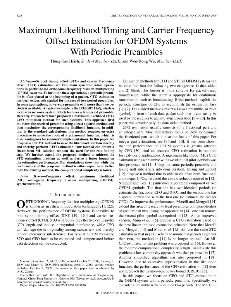
algorithms A′ and B are suboptimal. Table I summarizes thisresult. In Table I, MUL, ADD, LN, ABS, PH, and DIV denotethe multiplication, addition, natural logarithm, absolute value,phase derivation, and division operations, respectively. In ad-dition, the algorithm proposed in this section is referred to asproposed algorithm I, and the one in Section IV is termed pro-posed algorithm II. For the proposed algorithms, we considerthe worst case in which all the phase differences dr,s need tobe unwrapped. Fig. 1 shows several examples of how Q and Naffect the complexity. Note that the computational complexityfor the root-finding procedure in [17] is not included here.For convenience, we treat all operations other than addition asmultiplications. As we can see, the computational complexityfor the proposed algorithm is slightly lower than that foralgorithms A and B in [17], and algorithm A′ in [17] is thelowest. However, algorithm A′ truncates the polynomials withorder higher than two in (6), i.e., Λ(z) =

∑2m=−2 b(m)zm.

This impacts the estimation accuracy. Note that we can alwaystruncate the summation terms in (32) and thereby reduce thecomputational complexity of proposed algorithm I. Since sub-optimum approaches are not our focus, we will not consider thedetails here. We will now discuss the computational complexityof the root-finding procedure. As shown in [27] and [29], theroot-finding procedure requires O(K3) multiplications. Table Ishows that the computational complexity of algorithm A isO(NK2). Thus, the computational complexity of the root-finding procedure will be high when K is large. Furthermore,its implementation cost will also be higher, since we may needdedicated electronic circuitry to implement this function.

It is well known that the performance of an unbiased estima-tor is bounded by the CRLB [25]. If the variance of an unbiasedestimator reaches the CRLB, we consider the estimator effi-cient. Following the procedure to derive performance boundsin [25], we can calculate the CRLB for our CFO estimationprocedure. Let ε be an estimate of ε. The CRLB for our CFOestimation is then

CRLB(ε) = − 1

E[

∂2

∂ε2 Λ(ε)]

=(8π2ρ)−1σ2

w (1 + (K − 1)ρ)

E

[K−1∑p=1

K∑q>p

(q − p)2Re{γpqej2πε(q−p)

}]


Fig. 1. Computational complexity comparison for the algorithm in [17] and proposed algorithm I. Note that the complexity of the root-finding procedure is notconsidered in [17].

=σ2

w (1 + (K − 1)ρ)

8π2ρNσ2x

K−1∑p=1

K∑q>p

(q − p)2

=1 +K · SNR

8π2N · SNR2

1K−1∑p=1

K∑q>p

(q − p)2(36)

where E[·] denotes the expectation.

IV. PROPOSED JOINT ML STO AND CFO ESTIMATION

In this section, we extend the method developed in Section IIIto solve the STO-estimation problem. The core idea is to applya sliding data window for the received (Q+ 1)N samples;each window covers the preamble in the context of a particulartiming offset. We perform the ML CFO estimation for datain each window and store the estimated CFO and the corre-sponding maximum log-likelihood. Thereafter, the estimatedCFO with the largest log-likelihood is selected as the MLCFO estimate. The corresponding window position is takenas the ML STO estimate. Let the window size be QN , anddefine the set Vi = {y(i), y(i+ 1), . . . , y(i+QN − 1)} to bethe received data in window i. Since the maximum delay isshorter than N , it is clear that 0 ≤ i ≤ N − 1. If we let theSTO be θ, Vθ will cover the complete preamble. In Appendix B,

we show that the log-likelihood function for Vi can be ex-pressed by

Λi(ε) = Ci1 + Ci

2φi + Ci

3

Q−2∑p=0

Q−1∑q>p

∣∣γipq

∣∣ cos(ψi

pq

)(37)

where the superscript i indicates that all the variables arecalculated within Vi, and Ci

1, Ci2, and Ci

3 can be treated aswindow independent. Thus, we can simplify the above log-likelihood function using

Λi(ε) ≈ C2φi + C3

Q−2∑p=0

Q−1∑q>p

∣∣γipq

∣∣ cos(ψi

pq

)(38)

where C2 and C3 are the same as those in (23) and (24). Sincethe received signal power φi is independent of CFO, we canestimate CFO using (32) as

εi = −

Q−2∑p=0

Q−1∑q>p

∣∣γipq

∣∣ (q − p)∠γipq

2πQ−2∑p=0

Q−1∑q>p

|q − p|2 ∣∣γipq

∣∣ . (39)

Note that the upper bound in the summation terms of (39) is Qinstead of K. The estimated STO is then

θ = arg{

maxi

(Λi(εi)

)}= iopt. (40)


Now, the procedure for the proposed joint ML STO and CFOestimation can be summarized as follows.

1) Calculate γipq and its amplitude, where i ∈ [1, N ], p ∈

[0, Q− 2], and q ∈ [p+ 1, Q− 1].2) Use the phase unwrapping procedure outlined above to

calculate ∠γipq .

3) Substitute the results into (38) and (39), and calculateΛi(εi) and εi.

4) Find iopt such that Λiopt(εiopt) > Λi(εi), i �= iopt.5) The ML STO estimate is iopt, and the ML CFO estimate

is then εiopt .As we can see from the above procedure, the computationalcomplexity of the algorithm will be N times higher than thatin Section III. Note also that the upper limit of p is Q− 2instead of K − 2. In other words, we have an extra period forCFO estimation. By leveraging the sliding window structure,we can effectively reduce the computational complexity incalculating γi

pq. Similar to the definition of γpq, we obtain

γipq =

∑i+N−1n=i yp(n)[yq(n)]∗. Then, it is simple to show that

γipq = γi−1

pq + yp(i+N − 1) [yq(i+N − 1)]∗

−yp(i− 1) [yq(i− 1)]∗ . (41)

From (41), we can see that except for i = 0, the calculation ofγi

pq requires only two complex multiplications and two complexadditions. This will greatly reduce the required computationalcomplexity in the scenario of joint STO and CFO estimation.The required computational complexity has been summarizedin Table I.

We can also obtain the CRLB for the CFO estimate. All wehave to do is to replaceK withQ in (36). SinceQ = K + 1, theCRLB is lower than that in (36). Note that the STO is a discretevalue. No performance lower bounds have been reported to datein the literature. In Section V, we will derive a lower bound toaddress this omission.

V. PERFORMANCE ANALYSIS OF STO ESTIMATION

In this section, we analyze the performance of the proposedSTO estimation method. We first redefine (38) as Λi(ε) =C2φ

i + C3ξi, where

φi =K∑

p=0

i+N−1∑n=i

yp(n)y∗p(n)

=K∑

p=0

N−1∑n=0

xp(n)x∗p(n) + wp(n)w∗p(n)

+ 2Re{xp(n)w∗

p(n) exp(j2πε

pN + n

N

)}(42)

ξi =K−1∑p=0

K∑q>p

∣∣γipq

∣∣ cos(ψi

pq

)

=K−1∑p=0

K∑q>p

N−1∑n=0

xp(n)w∗q(n) exp

(j2πε

qN + n

N

)

+ wp(n)x∗q(n) exp(−j2πεpN + n

N

)+ wp(n)w∗

q(n) exp (j2πε(q − p)) + xp(n)x∗q(n). (43)

Note here that φi and ξi are random variables. The mean valueof Λi(ε), which is denoted by μi

Λ, is equal to C2μiφ + C3μ

iξ,

where μiφ and μi

ξ are the mean of φi and ξi, respectively.The variance of Λi can be expressed by νi

Λ = C22ν

iφ + C2

3νiξ +

2C2C3κiφξ, where νi

φ and νiξ denote the variance of φi and ξi,

respectively, and κiφξ the covariance between φi and ξi. The

whole set of Vi, 0 ≤ i ≤ N − 1, has (Q+ 1)N samples, and itmay cover three regions. The first region consists of the noisesamples, the second region the periodic preamble samples, andthe third region the data samples. We denote these regionsby IN , IP , and ID. Thus, the signal variance in IN is σ2

w,that in IP is σ2

x + σ2w, and that in ID is σ2

d + σ2w, where σ2

d

represents the variance of data samples. Recall that θ is theactual STO in the system. Using θ as a reference, we can havethe following three cases for the value of i: 1) i = θ; 2) i < θ;and 3) i > θ (0 ≤ i ≤ N − 1). The statistics of φi and ξi aredifferent across these three cases. In Appendix C, we provide adetailed derivation of μi

φ, μiξ, νi

φ, νiξ, and κi

φξ.For the proposed STO-estimation algorithm, an error occurs

when iopt �= θ. Thus, we can define the error probability ofSTO estimation as P (∪i,i �=θ{Λθ < Λi}), where P (·) denotesthe probability of a certain event. Note that the evaluationof P (Λθ < Λi) only requires 1-D integration. If the log-likelihood functions for all i’s are independent and identicallydistributed, we have P (∪i,i �=θ{Λθ < Λi}) =

∑i,i �=θ P (Λθ <

Λi). Unfortunately, the log-likelihood functions are not inde-pendent. As a result, we have to conduct multidimensionalintegration, which is both complex and difficult. Therefore, wepropose a simple alternative to overcome the problem. Insteadof the exact error probability, we attempt to derive a lowerbound.

As shown in [13], the likelihood function is approximatelyGaussian. We denote the distribution of Λi using G(μi

Λ, νiΛ),

where G(·) denotes the Gaussian distribution. Consider thejoint density function of Λi and Λj . Using the Gaussian as-sumption, we write the bivariate Gaussian distribution as

P (Λi,Λj) =1

2π · νiΛ · νj

Λ ·√1 − Cc(i, j)

· exp(− zij

2 (1 − Cc(i, j))

)(44)

where 1 ≤ i, j ≤ N , and

zij =

(Λi − μi

Λ

)2νiΛ

+

(Λj − μj

Λ

)2

νjΛ

−2Cc(i, j)

(Λi − μi

Λ

) (Λj − μj

Λ

)√νiΛ · νj

Λ

(45)

Cc(i, j) =E{Λi(Λj)∗

}− μiΛμ

j∗Λ√

νiΛ · νj

Λ

. (46)


Fig. 2. Comparison of simulated and theoretical P (Λθ > Λj).

Note that Cc(i, j) is the corresponding correlation coefficient.The numerator of Cc(i, j) is expressed as

E{Λi(Λj)∗

}= μi

Λμj∗Λ + C2

2κijφφ + C2

3κijξξ

+ C2C3κijφξ + C2C3κ

ijξφ (47)

where κijab denotes the covariance of ai and bj∗ (ai, bj ∈ {φi,

φj , ξi, ξj}). The main idea here is only to calculate P (Λθ >Λi) for all i’s (except for i = θ) and then use the result to derivea lower bound. Thus, we only have to consider Cc(i, θ) as

κiθφφ = 2σ2

xσ2w (QN − |i− θ|) (48)

κiθξξ =Q(Q− 1)σ2

xσ2w

[N

3(2Q− 1) − 1

2|i− θ|

]

+12QN(Q− 1)σ4

w (49)

κiθφξ =κiθ

ξφ = (Q− 1)2Nσ2xσ

2w

+ (Q− 1) (N − |i− θ|)σ2xσ

2w. (50)

Substituting (45)–(50) into (44), we can then evaluateP (Λθ > Λi). Given this definition, we have P (Λθ > Λi) =∫∞−∞∫ Λθ

−∞ P (Λi,Λθ)dΛidΛθ. Simulations have been conductedto evaluate the validity of our theoretical results. Using thescenario depicted in Section VI, we compare the theoreticaland simulated P (Λθ > Λi) in Fig. 2. In the figure, we see thatthe theoretical P (Λθ > Λi) is close to the simulated result. Ifwe let Pmin = min

i�=θP (Λθ > Λi), we can then treat Pmin as an

upper bound for the correct probability of STO estimation (i.e.,iopt = θ). Thus, we can then have a lower bound for the errorprobability of STO estimation (LBSTO) as 1 − Pmin.

VI. SIMULATIONS AND DISCUSSIONS

In this section, we report our simulation results, which eval-uate the performance of the proposed algorithms. We adopt aRayleigh multipath channel with an exponential power decayand five channel taps. The preamble, which is generated from a

Fig. 3. Performance comparison of CFO estimation, the algorithm in [17],and proposed algorithm I; SNR = 10 dB.

Fig. 4. BER comparison for systems with and without CFO.

frequency-domain binary-phase-shift-keying-modulated signal,has ten periods, and each period has 16 samples. The datafollowing the preamble are transmitted using a 16-quadratic-amplitude-modulation scheme. The mean square error (MSE)of the estimated CFO is used as a performance measure. We firstconsider the CFO-only estimation problem. In this case, the firstreceived N samples are discarded. As previously mentioned,we term the proposed approach for this scenario as algorithm I(as described in Section III). We compare the proposed MLestimator with that in [17]. One optimum algorithm (algorithmA) and two suboptimum algorithms (algorithm A′ and B) in[17] are simulated. Fig. 3 shows the simulation result for SNRat 10 dB. In the figure, we can see that the performances ofalgorithms A′ and B are poorer. Algorithm A and the proposedalgorithm offer a similar level of performance that is very closeto the CRLB. To evaluate the impact of CFO on system perfor-mance, we conduct simulations for systems with and withoutCFO. For the system with CFO, we first use the proposedmethod to estimate CFO and then conduct CFO compensation.Fig. 4 shows the BER comparison for ε = 0.2. As we can see in


Fig. 5. Performance comparison for CFO estimation, the algorithm in [17],and proposed algorithm II; SNR = 10 dB.

Fig. 6. Performance comparison for CFO estimation, the algorithm in [17],and proposed algorithms I and II; N = 16, and Q = 10.

the figure, the BER performance degrades slightly when CFOis present.

We then consider the case of the joint STO and CFO esti-mation process. In this case, discarding the first received Nsamples is not necessary. As a result, one additional pream-ble is available. This means that the proposed method mayoffer better performance compared with the previous scenario.However, the price we pay for the additional STO estimationis the increase in computational complexity. As mentioned,we name this approach proposed algorithm II (as explained inSection IV). Using a similar approach, the method in [17] canalso be used to estimate STO. However, its computational com-plexity increases much more than our method. Fig. 5 shows thesimulation result for the CFO estimate. The proposed methodoffers good performance. Only when CFO is very close to±0.5 does the performance of the proposed algorithms degrade.Fig. 6 shows the CFO estimation result for various SNRs. Inthe figure, we see that the proposed method still works wellfor SNRs as low as −5 dB. The algorithms in [17] perform

Fig. 7. Error probability of STO estimation (proposed algorithm II).

Fig. 8. Performance comparison for STO estimation (SNR = 2 and 10 dB).

well until SNR reaches −7 dB, which is somewhat betterthan the proposed algorithms. However, when SNR falls below−8 dB, the proposed algorithms again outperform those in[17]. This may be because the correlation matrix in (6) is verynoisy, and the roots therefore cannot be solved reliably. Fig. 7shows the error probability for the STO estimation. We observethat the derived lower bound for the STO estimation is tightwhen the SNR is high. Note that the error probability we de-fined is only relevant to performance evaluation. If the channelresponse is shorter than the CP (which is the typical case),we can always has some tolerance for the STO estimation.Thus, there is no need to calculate the exact channel delay.In real-world applications, it is a common practice to reducethe estimated STO by a couple of samples when conductingSTO compensation. Another property is that STO estimationperformance is not particularly impacted when CFO is close to0.5. In the literature, there exist a number of STO estimationmethods. We select the two algorithms proposed in [13] and[18] for comparison. Fig. 8 shows the MSE curves for theseapproaches and for the proposed algorithms (θ = 8). The figureconfirms that the proposed method performs best.


VII. CONCLUSION

In this paper, we have developed new algorithms for ML STOand CFO estimation in OFDM systems with periodic pream-bles. The proposed algorithms do not have to calculate theroots of the derivative of the likelihood function. The operationsare simple, and the computational complexity is low. With theproposed method, we can simultaneously solve the STO andCFO estimation problems. We also derive a lower bound forthe STO estimation error. Simulations show that the proposedmethods offer good performance, and the derived lower boundis tight when the SNR is high.

APPENDIX ADERIVATION OF (19)

The likelihood function in (18) can be rewritten as

Λ(ε) =N−1∑n=0

ln

⎧⎪⎪⎪⎪⎪⎪⎪⎪⎪⎪⎨⎪⎪⎪⎪⎪⎪⎪⎪⎪⎪⎩

(σ2

x + σ2w

)K exp[−y(n)HR−1

y y(n)]

det(Ry) exp

⎡⎢⎢⎣−

K∑p=1

yp(n)y∗p(n)

σ2x+σ2

w

⎤⎥⎥⎦

⎫⎪⎪⎪⎪⎪⎪⎪⎪⎪⎪⎬⎪⎪⎪⎪⎪⎪⎪⎪⎪⎪⎭

=N−1∑n=0

{ln[(σ2

x + σ2w

)K (det(Ry))−1]

+

K∑p=1

yp(n)y∗p(n)

σ2x + σ2

w

− y(n)HR−1y y(n)

}.

(51)

Then, by substituting (17) into (51), we derive the log-likelihood function as

Λ(ε) =N−1∑n=0

{ln

[(σ2

x + σ2w

)Kdet(Ry)

]+

K∑p=1

yp(n)y∗p(n)

σ2x + σ2

w

− (σ−2w − C0

) K∑p=1

yp(n)y∗p(n)

+ 2C0Re

{K−1∑p=1

K∑q>p


}}

=N−1∑n=0

{ln[(σ2

x + σ2w

)K (det(Ry))−1]

+[

1σ2

x + σ2w

− (σ−2w − C0

)] K∑p=1

yp(n)y∗p(n)

+ 2C0Re

{K−1∑p=1

K∑q>p


}}

=(1 −K)σ4

x

σ2w (σ2

x + σ2w) (Kσ2

x + σ2w)

K∑p=1

N−1∑n=0

yp(n)y∗p(n)

+ 2C0Re

{K−1∑p=1

K∑q>p

N−1∑n=0


}

+N{

ln[(σ2

x + σ2w

)K (det(Ry))−1]}

(52)

where C0 = σ2x/(σ

4w +Kσ2

wσ2x). By substituting (21) and (25)

into (52), we can express (52) as

Λ(ε) =C1 + C2

K∑p=1

γpp

+ C3Re

{K−1∑p=1

K∑q>p

γpqej2π(q−p)ε

}

=C1 + C2

K∑p=1

γpp

+ C3Re

{K−1∑p=1

K∑q>p

(|γpq|ej∠γpq)ej2π(q−p)ε

}

=C1 + C2φ+ C3

K−1∑p=1

K∑q>p

|γpq| cos(ψpq) (53)

where ψpq, φ, C1, C2, and C3 are defined as (22)–(24).

APPENDIX BDERIVATION OF (38)

We assume that the channel noise, the received preamble,and the received data are statistically uncorrelated with oneanother. We define three column vectors y1(n) = [y0(n), . . . ,yQ−1(n)]T , y2(n) = [y1(n), . . . , yQ−1(n)]T , and y3(n) =[y0(n), . . . , yQ−2(n)]T and their autocorrelation matrix as Ryk

for k = 1, 2, and 3. Note that i is the window index of (37),and θ is the real STO. Therefore, (19) can be derived for thefollowing two cases: 1) i ≤ θ and 2) i > θ. Using the approachtaken to derive (18), we obtain the log-likelihood function forthe first case as

Λi≤θ(ε) = ln

⎧⎪⎪⎪⎨⎪⎪⎪⎩

n=i+N−1∏n=i

f (y(n))Q∏

k=1

f (yk−1(n))

⎫⎪⎪⎪⎬⎪⎪⎪⎭

=θ−1∑n=i

ln{

f (y2(n))f (y1(n)) · · · f (yQ−1(n))

}

+i+N−1∑

n=θ

ln{

f (y1(n))f (y0(n)) · · · f (yQ−1(n))

}(54)

=θ − i

NC12 +

i+N − θ

NC ′

1

+θ−1∑n=i

C2

Q−1∑p=1

yp(n)y∗p(n)


+θ−1∑n=i

C3Re

{Q−2∑p=1

Q−1∑q>p


}

+i+N−1∑

n=θ

C ′3Re

{Q−2∑p=0

Q−1∑q>p


}

+i+N−1∑

n=θ

C ′2

Q−1∑p=0

yp(n)y∗p(n) (55)

where

C12 =N · ln((

σ2x + σ2

w

)Kdet(Ry2)

)(56)

C ′1 =N · ln

((σ2

x + σ2w

)Qdet(Ry1)

)(57)

C ′2 = (1 −Q)

ρ2

σ2w (1 + (Q− 1)ρ)

(58)

C ′3 = =,

2C ′2

(1 −Q)ρ. (59)

Similarly, we can derive the log-likelihood function fori > θ as

Λi>θ(ε) =i+N−1∑n=θ+N

ln{

f (y3(n))f (y0(n)) · · · f (yQ−2(n))

}

+θ+N−1∑

n=i

ln{

f (y1(n))f (y0(n)) · · · f (yQ−1(n))

}(60)

=i− θ

NC13 +

θ +N − i

NC ′

1

+i+N−1∑n=θ+N

C2

Q−2∑p=0

yp(n)y∗p(n)

+i+N−1∑n=θ+N

C3Re

{Q−3∑p=0

Q−2∑q>p


}

+θ+N−1∑

n=i

C ′2

Q−1∑p=0

yp(n)y∗p(n)

+θ+N−1∑

n=i

C ′3Re

{Q−2∑p=0

Q−1∑q>p


}

(61)

where

C13 = N · ln((

σ2x + σ2

w

)Kdet(Ry3)

).

Since y2(n), i ≤ n ≤ θ − 1 in (54) and y3(n), θ +N ≤ n ≤i+N − 1 in (60) contain Q− 1 periods of the preamble,det(Ry2) and det(Ry3) will be the same as det(Ry) [see (22)].Consequently, C12 = C13 = C1. From (22)–(24), we see thatC1, C2, and C3 can be calculated by replacing Q and Ry1 with

K and Ry , respectively, in (57)–(59). When Q is reasonablylarge, we obtain C ′

1 ≈ C1, C ′2 ≈ C2, and C ′

3 ≈ C3. Thus, werewrite (55) and (61) as

Λi≤θ(ε) θ−1∑n=i

C3Re

{Q−2∑p=1

Q−1∑q>p


}

+i+N−1∑

n=θ

C3Re

{Q−2∑p=0

Q−1∑q>p


}

+ C1 +θ−1∑n=i

C2

Q−1∑p=1

yp(n)y∗p(n)

+i+N−1∑

n=θ

C2

Q−1∑p=0

yp(n)y∗p(n) (62)

Λi>θ(ε) θ+N−1∑

n=i

C3Re

{Q−2∑p=0

Q−1∑q>p


}

+i+N−1∑n=θ+N

C3Re

{Q−3∑p=0

Q−2∑q>p


}

+ C1 +i+N−1∑n=θ+N

C2

Q−2∑p=0

yp(n)y∗p(n)

+θ+N−1∑

n=i

C2

Q−1∑p=0

yp(n)y∗p(n). (63)

We now approximate∑Q−1

p=1 yp(n)y∗p(n) and∑Q−2

p=1

∑Q−1q>p ×

yp(n)y∗q(n)ej2π(q−p)ε in (62) with∑Q−1

p=0 yp(n)y∗p(n)and

∑Q−2p=0

∑Q−1q>p yp(n)y∗q(n)ej2π(q−p)ε, respectively.

Similarly, we also approximate∑Q−2

p=0 yp(n)y∗p(n)and

∑Q−3p=0

∑Q−2q>p yp(n)y∗q(n)ej2π(q−p)ε in (63) with∑Q−1

p=0 yp(n)y∗p(n) and∑Q−2

p=0

∑Q−1q>p yp(n)y∗q(n)ej2π(q−p)ε,

respectively. Given these approximations, Λi≤θ(ε) and Λi>θ(ε)can be identically written as

Λi(ε) C1 + C2

i+N−1∑n=i

Q−1∑p=0

yp(n)y∗p(n)

+C3

i+N−1∑n=i

Re

{Q−2∑p=0

Q−1∑q>p


}. (64)

Using the approach that is similar to that in Appendix A, wefinally obtain

Λi(ε) C1 + C2φi + C3Re

{Q−2∑p=0

Q−1∑q>p

∣∣γipq

∣∣ cos(ψi

pq

)}

(65)

where γipq =

∑i+N−1n=i yp(n)y∗q(n), φi =

∑Q−1p=0 γ

ipp, and

ψipq = 2πε(q − p) + ∠γi

pq . Note that the approximations wemade are equivalent to adding |θ − i| samples (noise or data)


in calculating the likelihood functions. Since the numberof samples in the ith sliding data window QN is usuallymuch larger than the number of added samples |θ − i|, theadded samples will not change the likelihood functions toomuch. The approximation errors also depend on the distancebetween the window position and the actual STO, i.e., |θ − i|.When the distance is larger, the error is also larger. However,if the distance is larger, the likelihood function tends to besmaller, and a larger error is then tolerable. Finally, we notethat the added samples, either noise or data, are uncorrelatedwith the preamble samples.

APPENDIX CDERIVATIONS OF μi

φ , μiξ , νi

φ, νiξ , AND κi

φξ

We first note that θ is the real STO in the system. Using θ asa reference, we have the following three cases for the value of i:1) i = θ; 2) i < θ; and 3) i > θ (0 ≤ i ≤ N − 1). For the firstcase, the window covers the preamble data only (IP ). Thus,(42) and (43) can be simplified to

φθ =Q−1∑p=0

θ+N−1∑n=θ


+ 2Re{xp(n)w∗

p(n) exp(j2πε

pN + n

N

)}(66)

ξθ =Q−2∑p=0

Q−1∑q>p

θ+N−1∑n=θ

xp(n)x∗q(n)

+ xp(n)w∗q(n) exp

(j2πε

qN + n

N

)


N

)

+ wp(n)w∗q(n) exp (j2πε(q − p)) . (67)

The mean values of φi and ξi for the first case are then

μθφ,1 =QN

(σ2

x + σ2w

)(68)

μθξ,1 =

QN(Q− 1)2

σ2x. (69)

The corresponding variance values are

νθφ,1 = 2QN

(σ2

xσ2w

)(70)

νθξ,1 =

QN(Q− 1)2

σ4w

+ σ2xσ

2w

QN(Q− 1)(2Q− 1)3

. (71)

The corresponding covariance value is

κθφξ,1 = QN(Q− 1)

(σ2

xσ2w

). (72)

Here, κiφξ,j denotes κi

φξ in the jth case discussed. For thesecond case, the window covers the sets IN and IP . Thus, φi

and ξi can be expressed as

φi =θ−1∑n=i

w0(n)w∗0(n)

+i+N−1∑

n=θ

x0(n)x∗0(n) + w0(n)w∗0(n)

+ 2Re{x0(n)w∗

0(n) exp(j2πε

n

N

)}

+Q−1∑p=1

i+N−1∑n=i


+ 2Re{xp(n)w∗

p(n) exp(j2πε

pN + n

N

)}(73)

ξi =Q−1∑q>0

θ−1∑n=i

w0(n)x∗q(n) exp(−j2πε n

N

)+ w0(n)w∗

q(n) exp(j2πεq)

+Q−1∑q>0

N+i−1∑n=θ

x0(n)x∗q(n)

+ x0(n)w∗q(n) exp

(j2πε

qN + n

N

)

+ w0(n)x∗q(n) exp(−j2πε n

N

)+ w0(n)w∗

q(n) exp(j2πεq)

+Q−2∑p=1

Q−1∑q>p

i+N−1∑n=i

xp(n)x∗q(n)

+ xp(n)w∗q(n) exp

(j2πε

qN + n

N

)


N

)+ wp(n)w∗

q(n) exp (j2πε(q − p)) . (74)

Their mean values are

μiφ,2 = (QN + i− θ)

(σ2

x + σ2w

)+ (i− θ)σ2

x (75)

μiξ,2 = (Q− 1)(N + i− θ)σ2

x

+(Q− 1)(Q− 2)

2Nσ2

x (76)

the corresponding variance values are

νiφ,2 = 2σ2

xσ2w[QN + i− θ] (77)

νiξ,2 =

QN(Q− 1)2

σ4w + σ2

xσ2wN(Q− 1)

·[(Q− 1)

(2 +

i− θ

N

)+

(Q− 2)(2Q− 3)3

](78)

and the covariance value is

κiφξ,2 = (QN + i− θ)(Q− 1)

(σ2

xσ2w

). (79)


For the third case, the window covers sets IP and ID, and wewrite φi and ξi as

φi =Q−2∑p=0

i+N−1∑n=i

{xp(n)x∗p(n) + wp(n)w∗

p(n) + 2Re

×[xp(n)w∗

p(n) exp(j2πε

pN + n

N

)]}

+θ+N−1∑

n=i

{xQ−1(n)x∗Q−1(n) + wQ−1(n)w∗

Q−1(n)

+ 2Re

[xQ−1(n)w∗

Q−1(n)

× exp(j2πε

(Q− 1)N + n

N

)]}

+i+N−1∑n=θ+N

{xQ−1(n)x∗Q−1(n) + wQ−1(n)w∗

Q−1(n)

+ 2Re

[xQ−1(n)w∗

Q−1(n)

× exp(j2πε

(Q− 1)N + n

N

)]}

(80)

ξi =Q−3∑p=0

Q−2∑q>p

i+N−1∑n=i

xp(n)x∗q(n)

+ xp(n)w∗q(n) exp

(j2πε

qN + n

N

)


N

)+ wp(n)w∗

q(n) exp (j2πε(q − p))

+Q−2∑p=0

θ+N−1∑n=i

xp(n)x∗Q−1(n)

+ xp(n)w∗Q−1(n) exp

(j2πε

(Q− 1)N + n

N

)

+ wp(n)x∗Q−1(n) exp(−j2πεpN + n

N

)+ wp(n)w∗

Q−1(n) exp (j2πε(Q− p− 1))

+Q−2∑p=0

i+N−1∑n=θ+N

xp(n)x∗Q−1(n)

+ xp(n)w∗Q−1(n) exp

(j2πε

(Q− 1)N + n

N

)

+ wp(n)x∗Q−1(n) exp(−j2πεpN + n

N

)+ wp(n)w∗

Q−1(n) exp (j2πε(Q− p− 1)) . (81)

Thus, the mean values are

μiφ,3 = (QN + θ − i)

(σ2

x + σ2w

)+ (i− θ)

(σ2

d + σ2w

)(82)

μiξ,3 = (Q− 1)(N − i+ θ)σ2

x +(Q− 1)(Q− 2)

2Nσ2

x (83)

the variance values are

νiφ,3 = 2σ2

xσ2w(QN − i+ θ) + 2(i− θ)σ2

dσ2w (84)

νiξ,3 =σ2

xσ2wN(Q− 1)

×[(2Q− 3)

(1 +

θ − i

N

)+

(Q− 2)(2Q− 3)3

+ 1]

+QN(Q− 1)

2σ4

w + (Q− 1)2(i− θ)(σ2d + σ2

w) (85)

and the covariance value is

κiφξ,3 = (Q− 1)σ2

xσ2w [QN + 2(θ − i)] . (86)

REFERENCES

[1] J. J. van de Beek, M. Sandell, and P. O. Borjesson, “ML estimation of timeand frequency offset in OFDM systems,” IEEE Trans. Signal Process.,vol. 45, no. 7, pp. 1800–1805, Jul. 1997.

[2] N. Lashkarian, “Class of cyclic-based estimators for frequency-offsetestimation of OFDM systems,” IEEE Trans. Commun., vol. 48, no. 12,pp. 2139–2149, Dec. 2000.

[3] Y.-C. Wu and E. Serpedin, “Comments on ‘Class of cyclic-based esti-mators for frequency-offset estimation of OFDM systems,”’ IEEE Trans.Commun., vol. 53, no. 3, pp. 413–414, Mar. 2005.

[4] M. Tanda, “Blind symbol-timing and frequency-offset estimation inOFDM systems with real data symbols,” IEEE Trans. Commun., vol. 52,no. 10, pp. 1609–1612, Oct. 2004.

[5] H. Meyr, M. Moeneclaey, and S. A. Fechtel, Digital CommunicationReceivers: Synchronization, Channel Estimation, and Signal Processing.New York: Wiley, 1998.

[6] E. Chiavaccini and G. M. Vitetta, “Maximum-likelihood frequency re-covery for OFDM signals transmitted over multipath fading channels,”IEEE Trans. Commun., vol. 52, no. 2, pp. 244–251, Feb. 2004.

[7] D. Lee and K. Cheun, “Coarse symbol synchronization algorithms forOFDM systems in multipath channels,” IEEE Commun. Lett., vol. 6,no. 10, pp. 446–448, Oct. 2002.

[8] S. Haykin, Adaptive Filter Theory 4E. Englewood Cliffs, NJ:Prentice–Hall, 2002, p. 440.

[9] M. Morelli, A. N. D’Andrea, and U. Mengali, “Frequency ambiguityresolution in OFDM systems,” IEEE Commun. Lett., vol. 4, no. 4,pp. 134–136, Apr. 2000.

[10] K.-T. Lee and J.-S. Seo, “Pilot-aided iterative frequency offset estimationfor digital video broadcasting (DVB) systems,” IEEE Trans. Consum.Electron., vol. 53, no. 1, pp. 11–16, Feb. 2007.

[11] P. H. Moose, “A technique of orthogonal frequency division multiplexingfrequency offset correlation,” IEEE Trans. Commun., vol. 42, no. 10,pp. 2908–2914, Oct. 1994.

[12] D. Huang and K. B. Letaief, “Carrier frequency offset estimation forOFDM systems using null subcarriers,” IEEE Trans. Commun., vol. 54,no. 5, pp. 813–823, May 2006.

[13] T. M. Schmidl and D. C. Cox, “Robust frequency and timing synchroniza-tion for OFDM,” IEEE Trans. Commun., vol. 45, no. 12, pp. 1613–1621,Dec. 1997.

[14] M. Morelli and U. Mengali, “An improved frequency offset estimatorfor OFDM applications,” IEEE Commun. Lett., vol. 3, no. 3, pp. 75–77,Mar. 1999.

[15] H. Minn, P. Tarasak, and V. K. Bhargava, “OFDM frequency offset esti-mation methods based on BLUE principle,” in Proc. IEEE Veh. Technol.Conf., Vancouver, BC, Canada, Sep. 2002, pp. 1230–1234.

[16] J. Li, G. Liu, and G. B. Giannakis, “Carrier frequency offset estimationfor OFDM-based WLANs,” IEEE Signal Process. Lett., vol. 8, no. 3,pp. 80–82, Mar. 2001.


[17] J. H. Yu and Y. T. Su, “Pilot-assisted maximum-likelihood frequency-offset estimation for OFDM systems,” IEEE Trans. Commun., vol. 52,no. 11, pp. 1997–2008, Nov. 2004.

[18] M. H. Cheng and C. C. Chou, “Maximum-likelihood estimation of fre-quency and time offsets in OFDM systems with multiple sets of identi-cal data,” IEEE Trans. Signal Process., vol. 54, no. 7, pp. 2848–2852,Jul. 2006.

[19] W. D. Warner and C. Leung, “OFDM/FM frame synchronization formobile radio data communication,” IEEE Trans. Veh. Technol., vol. 42,no. 3, pp. 302–313, Aug. 1993.

[20] L. Hanzo, “Bandwidth-efficient wireless multimedia communications,”Proc. IEEE, vol. 86, no. 7, pp. 1342–1382, Jul. 1998.

[21] R. van Nee and R. Prasad, OFDM for Wireless Multimedia Commu-nications. Boston, MA: Artech House, 2002.

[22] J. Heiskala and J. Terry, OFDM Wireless LANs: A Theoretical and Prac-tical Guide. Indianapolis, IN: Sams, 2002.

[23] Y. S. Choi, P. J. Voltz, and F. A. Cassara, “ML estimation of carrierfrequency offset for multicarrier signals in Rayleigh fading channels,”IEEE Trans. Veh. Technol., vol. 50, no. 2, pp. 644–655, Mar. 2001.

[24] S. M. Kay, Fundamentals of Statistical Signal Processing: EstimationTheory. Englewood Cliffs, NJ: Prentice–Hall, 1993.

[25] H. V. Poor, An Introduction to Signal Detection and Estimation 2E.Berlin, Germany: Springer-Verlag, 1994.

[26] P. Stoica and A. Nehorai, “MUSIC, maximum likelihood, and Cramer–Rao bound,” IEEE Trans. Acoust., Speech, Signal Process., vol. 37, no. 5,pp. 720–741, May 1989.

[27] Y. Jian, H. Minn, X. Gao, X. You, and Y. Li, “Frequency offset estimationand training sequence design for MIMO OFDM,” IEEE Trans. WirelessCommun., vol. 7, no. 4, pp. 1244–1254, Apr. 2008.

[28] S. Tretter, “Estimating the frequency of a noisy sinusoid by linear re-gression,” IEEE Trans. Inf. Theory, vol. IT-31, no. 6, pp. 832–835,Nov. 1985.

[29] W. S. McCormick and L. L. James, “Efficient parallel rooting of complexpolynomials on the unit circle,” IEEE Trans. Signal Process., vol. 39,no. 10, pp. 2347–2351, Oct. 1991.

[30] L. Rugini and P. Banelli, “BER of OFDM systems imparied by carrierfrequency offset in multipath fading channels,” IEEE Trans. WirelessCommun., vol. 4, no. 5, pp. 2279–2288, Sep. 2008.

Hung-Tao Hsieh (S’08) received the B.S. degreein physics in 2000 from the National Central Uni-versity, Taoyuan, Taiwan, and the M.S. degree inelectro-physics in 2002 from the National ChiaoTung University (NCTU), Hsinchu, Taiwan, wherehe is currently working toward the Ph.D. degree withthe Department of Communication Engineering.

His research interests include detection/estimationtheories and communication signal processing.

Wen-Rong Wu (M’89) received the B.S. degreein mechanical engineering from Tatung Instituteof Technology, Taipei, Taiwan, in 1980 and theM.S. degrees in mechanical and electrical engineer-ing and the Ph.D. degree in electrical engineeringfrom the State University of New York, Buffalo,in 1985, 1986, and 1989, respectively.

Since August 1989, he has been a faculty memberwith the Department of Communication Engineer-ing, National Chiao Tung University, Hsinchu,Taiwan. His research interests include statistical

signal processing and digital communication.

Documents

Maximum Likelihood Timing and Carrier Frequency … IEEE TRANSACTIONS ON VEHICULAR TECHNOLOGY, VOL. 58, NO. 8, OCTOBER 2009 Maximum Likelihood Timing and Carrier Frequency Offset Estimation