Maximum Likelihood Estimation of a Stochastic Integrate-and-Fire

LETTER Communicated by Anthony Burkitt

Maximum Likelihood Estimation of a StochasticIntegrate-and-Fire Neural Encoding Model

Liam [email protected] Hughes Medical Institute, Center for Neural Science, New York University,New York, NY 10003, U.S.A., and Gatsby Computational Neuroscience Unit,University College London, London WC1N 3AR, U.K.

Jonathan W. [email protected] Hughes Medical Institute, Center for Neural Science, New York University,New York, NY 10003, U.S.A.

Eero P. [email protected] Hughes Medical Institute, Center for Neural Science, and Courant Institutefor Mathematical Science, New York University, New York, NY 10003, U.S.A.

We examine a cascade encoding model for neural response in which a lin-ear filtering stage is followed by a noisy, leaky, integrate-and-fire spikegeneration mechanism. This model provides a biophysically more realis-tic alternative to models based on Poisson (memoryless) spike generation,and can effectively reproduce a variety of spiking behaviors seen in vivo.We describe the maximum likelihood estimator for the model parameters,given only extracellular spike train responses (not intracellular voltagedata). Specifically, we prove that the log-likelihood function is concaveand thus has an essentially unique global maximum that can be foundusing gradient ascent techniques. We develop an efficient algorithm forcomputing the maximum likelihood solution, demonstrate the effective-ness of the resulting estimator with numerical simulations, and discuss amethod of testing the model’s validity using time-rescaling and densityevolution techniques.

1 Introduction

A central issue in systems neuroscience is the experimental characterizationof the functional relationship between external variables, such as sensorystimuli or motor behavior, and neural spike trains. Because neural responsesto identical experimental input conditions are variable, we frame the prob-lem statistically: we want to estimate the probability of any spiking response

Neural Computation 16, 2533–2561 (2004) c© 2004 Massachusetts Institute of Technology

2534 L. Paninski, J. Pillow, and E. Simoncelli

conditioned on any input. Of course, there are typically far too many possi-ble observable signals to measure these probabilities directly. Thus, our realgoal is to find a good model—some functional form that allows us to pre-dict spiking probability even for signals we have never observed directly.Ideally, such a model will be both accurate in describing neural responseand easy to estimate from a modest amount of data.

A good deal of recent interest has focused on models of cascade type.These models consist of a linear filtering stage in which the observable sig-nal is projected onto a low-dimensional subspace, followed by a nonlinear,probabilistic spike generation stage. The linear filtering stage is typicallyinterpreted as the neuron’s “receptive field,” efficiently representing the rel-evant information contained in the possibly high-dimensional input signal,while the spiking mechanism accounts for simple nonlinearities like rectifi-cation and response saturation. Given a set of stimuli and (extracellularly)recorded spike times, the characterization problem consists of estimatingboth the linear filter and the parameters governing the spiking mechanism.Unfortunately, biophysically realistic models of spike generation, such asthe Hodgkin-Huxley model or its variants (Koch, 1999), are generally quitedifficult to fit given only extracellular data.

As such, it has become common to assume a highly simplified model inwhich spikes are generated according to an inhomogeneous Poisson pro-cess, with rate determined by an instantaneous (“memoryless”) nonlinearfunction of the linearly filtered input (see Simoncelli, Paninski, Pillow, &Schwartz, in press, for review and partial list of references). In addition toits conceptual simplicity, this linear-nonlinear-poisson (LNP) cascade modelis computationally tractable. In particular, reverse correlation analysis pro-vides a simple unbiased estimator for the linear filter (Chichilnisky, 2001),and the properties of estimators for both the linear filter and static nonlin-earity have been thoroughly analyzed, even for the case of highly nonsym-metric or “naturalistic” stimuli (Paninski, 2003). Unfortunately, however,memoryless Poisson processes do not readily capture the fine temporalstatistics of neural spike trains (Berry & Meister, 1998; Keat, Reinagel, Reid,& Meister, 2001; Reich, Victor, & Knight, 1998; Aguera y Arcas & Fairhall,2003). In particular, the probability of observing a spike is not a functional ofthe recent stimulus alone; it is also strongly affected by the recent history ofspiking. This spike history dependence can significantly bias the estimationof the linear filter of an LNP model (Berry & Meister, 1998; Pillow & Simon-celli, 2003; Paninski, Lev, & Reyes; 2003; Paninski, 2003; Aguera y Arcas &Fairhall, 2003).

In this letter, we consider a model that provides an appealing compro-mise between the oversimplified Poisson model and more biophysicallyrealistic but intractable models for spike generation. The model consists ofa linear filter (L) followed by a probabilistic, or noisy (N), form of leakyintegrate-and-fire (LIF) spike generation (Koch, 1999). This L-NLIF modelis illustrated in Figure 1, and is essentially the standard LIF model driven

ML Estimation of a Stochastic Integrate-and-Fire Model 2535

��

��

��

��

��

��

�

Figure 1: Illustration of the L-NLIF model.

by a noisy, filtered version of the stimulus; the spike history dependenceintroduced by the integrate-and-fire mechanism allows the model to emu-late many of the spiking behaviors seen in real neurons (Gerstner & Kistler,2002). This model thus combines the encoding power of the LNP cell withthe flexible spike history dependence of the LIF model and allows us toexplicitly model neural firing statistics.

Our main result is that the estimation of the L-NLIF model parameters iscomputationally tractable. Specifically, we formulate the problem in termsof classical estimation theory, which provides a natural “cost function” (like-lihood) for model assessment and estimation of the model parameters. Wedescribe algorithms for computing the likelihood function and prove thatthis likelihood function contains no nonglobal local maxima, implying thatthe maximum likelihood estimator (MLE) can be computed efficiently usingstandard ascent techniques. Desirable statistical properties of the estimator(such as consistency and efficiency) are all inherited “for free” from classi-cal estimation theory (van der Vaart, 1998). Thus, we have a compact andpowerful model for the neural code and a well-motivated, efficient way toestimate the parameters of this model from extracellular data.

2 The Model

We consider a model for which the (dimensionless) subthreshold voltagevariable V evolves according to

dV = (−g(V(t) − Vleak) + Istim(t) + Ihist(t))dt + Wt, (2.1)

and resets instantaneously to Vreset < 1 whenever V = 1, the thresholdpotential (see Figure 2). Here, g denotes the membrane leak conductance,Vleak the leak reversal potential, and the stimulus current Istim is defined as

Istim(t) = �k · �x(t),


� ��

��

��

��

��

�

��

�

��

�

��

�

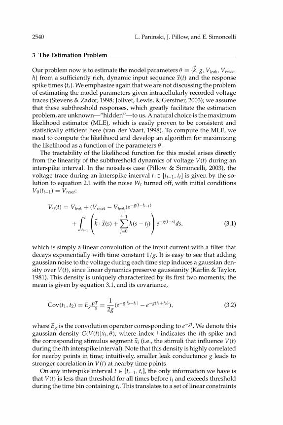
Figure 2: Behavior of the L-NLIF model during a single interspike interval, fora single (repeated) input current. (Top) Observed stimulus x(t) and responsespikes. (Third panel) Ten simulated voltage traces V(t), evaluated up to the firstthreshold crossing, conditional on a spike at time zero (Vreset = 0). Note thestrong correlation between neighboring time points, and the gradual sparsen-ing of the plot as traces are eliminated by spiking. (Fourth panel) Evolution ofP(V, t). Each vertical cross section represents the conditional distribution of V atthe corresponding time t (i.e., for all traces that have not yet crossed threshold).Note the boundary conditions P(Vth, t) = 0 and P(V, tspike) = δ(V − Vreset) cor-responding to threshold and reset, respectively. See section 4 for computationaldetails. (Bottom panel) Probability density of the interspike interval (ISI) corre-sponding to this particular input. Note that probability mass is concentrated atthe times when input drives the mean voltage V0(t) close to threshold. Carefulexamination reveals, in fact, that peaks in p(ISI) are sharper than peaks in thedeterministic signal V0(t), due to the elimination of threshold-crossing tracesthat would otherwise have contributed mass to p(ISI) at or after such peaks(Berry & Meister, 1998).


the projection of the input signal �x(t) onto the spatiotemporal linear kernel�k; the spike-history current Ihist is given by

Ihist(t) =i−1∑j=0

h(t − tj),

where h is a postspike current waveform of fixed amplitude and shape1

whose value depends on only the time since the last spike ti−1 (with thesum above including terms back to t0, the first observed spike); finally,Wt is an unobserved (hidden) noise process, taken here to be a standardgaussian white noise (although we will consider more general Wt later). Asusual, in the absence of input, V decays back to Vleak with time constant1/g. Thus, the nonlinear behavior of the model is completely determinedby only a few parameters, namely, {g, Vreset, Vleak}, and h(t). In practice, weassume the continuous aftercurrent h(t) may be written as a superpositionof a small number of fixed temporal basis functions; we will refer to thevector of coefficients in this basis using the vector �h. We should note that theinclusion of the Ihist current in equation 2.1 introduces additional parameters(namely, �h) to the model that need to be fit; in cases where there is insufficientdata to properly fit these extra parameters, �h could be set to zero, reducingthe model, equation 2.1, to the more standard LIF setting.

It is important to emphasize that in the following, V(t) itself will beconsidered a hidden variable; we are assuming that the spike train datawe are trying to model have been collected extracellularly, without anyaccess to the subthreshold voltage V. This implies that the parameters ofthe usual LIF model can only be estimated up to an unlearnable mean andscale factor. Thus, by a standard change of variables, we have not lost anygenerality by setting the threshold potential, Vth, and scale of the hiddennoise process, σ , to 1 (corresponding to mapping the physical voltage V →1 + (V − Vth)/σ ); the relative noise level (the effective scale of Wt) can bechanged by scaling Vleak, Vreset, �k, and h together. Of course, other changesof variable are possible (e.g., letting σ change freely and fixing Vreset = 0),but will not affect the analysis here.

The dynamical properties of this type of “spike response model” havebeen extensively studied (Gerstner & Kistler, 2002); for example, it is knownthat this class of models can effectively capture much of the behavior of ap-parently more biophysically realistic models (e.g., Hodgkin-Huxley). Weillustrate some of these diverse firing properties in Figures 3 and 4. Thesefigures also serve to illustrate several of the important differences betweenthe L-NLIF and LNP models. In Figure 3, note the fine structure of spiketiming in the responses of the L-NLIF model, which is qualitatively similarto in vivo experimental observations (Berry and Meister, 1998; Reich et al.,

1 The letter h here was chosen to stand for “history” and should not be confused withthe physiologically defined Ih current.


Figure 3: Simulated responses of L-NLIF and LNP models to 20 repetitions ofa fixed 100-ms stimulus segment of temporal white noise. (Top) Raster of re-sponses of L-NLIF model to a dynamic input stimulus. The top row shows thefixed (deterministic) response of the model with the noise set to zero. (Mid-dle) Raster of responses of LNP model to the same stimulus, with parametersfit with standard methods from a long run of the L-NLIF model responses tononrepeating stimuli. (Bottom) Poststimulus time histogram (PSTH) of the sim-ulated L-NLIF response (black line) and PSTH of the LNP model (gray line).Note that the LNP model, due to its Poisson output structure, fails to preservethe fine temporal structure of the spike trains relative to the L-NLIF model.

1998; Keat et al., 2001). The LNP model fails to capture this fine temporalreproducibility. At the same time, the L-NLIF model is much more flex-ible and representationally powerful: by varying Vreset or h, for example,we can match a wide variety of interspike interval distributions and firing-rate curves, even given a single fixed stimulus. For example, the model canmimic the FI curves of type I or II models, with either smooth or discontinu-ous growth of the FI curve away from 0 at threshold, respectively (Gerstner& Kistler, 2002). More generally, the L-NLIF model can exhibit adaptive be-havior (Rudd & Brown, 1997; Paninski, Lau, & Reyes, 2003; Yu & Lee, 2003)and display rhythmic, tonic, or even bistable dynamical behavior, depend-ing on the parameter settings (see Figure 4).


��

��

��

��

��

�

��

��

��

�

�

��

�

�

�

�

�

�

��

��

��

��

�

��

��

�

��

�

��

�

��

��

��

�

�

Figure 4: Diversity of NLIF model response patterns. (A) Firing-rate adapta-tion. A positive DC current was injected into three different NLIF cells, all withslightly different settings for h (top, h = 0; middle, h hyperdepolarizing; bottom,h depolarizing). Note that all three voltage response traces are identical until thetime of the first spike, but adapt to the constant input in three different ways.(For clarity, the noise level is set to zero in all panels.) (B) Rhythmic, burstingresponses. DC current (top trace) injected into an NLIF cell with h shown atleft. As amplitude c of current increases (voltage traces, top to bottom), burstfrequency and duration increase. (C) Tonic and bistable (“memory”) responses.The same current (top trace) was injected into two different NLIF cells with dif-ferent settings for h. The biphasic h in the bottom panel leads to a self-sustainingresponse that is inactivated only by the subsequent negative pulse.


3 The Estimation Problem

Our problem now is to estimate the model parameters θ ≡ {�k, g, Vleak, Vreset,

h} from a sufficiently rich, dynamic input sequence �x(t) and the responsespike times {ti}. We emphasize again that we are not discussing the problemof estimating the model parameters given intracellularly recorded voltagetraces (Stevens & Zador, 1998; Jolivet, Lewis, & Gerstner, 2003); we assumethat these subthreshold responses, which greatly facilitate the estimationproblem, are unknown—“hidden”—to us. A natural choice is the maximumlikelihood estimator (MLE), which is easily proven to be consistent andstatistically efficient here (van der Vaart, 1998). To compute the MLE, weneed to compute the likelihood and develop an algorithm for maximizingthe likelihood as a function of the parameters θ .

The tractability of the likelihood function for this model arises directlyfrom the linearity of the subthreshold dynamics of voltage V(t) during aninterspike interval. In the noiseless case (Pillow & Simoncelli, 2003), thevoltage trace during an interspike interval t ∈ [ti−1, ti] is given by the so-lution to equation 2.1 with the noise Wt turned off, with initial conditionsV0(ti−1) = Vreset:

V0(t) = Vleak + (Vreset − Vleak)e−g(t−ti−1)

+∫ t

ti−1

�k · �x(s) +

i−1∑j=0

h(s − tj)

e−g(t−s)ds, (3.1)

which is simply a linear convolution of the input current with a filter thatdecays exponentially with time constant 1/g. It is easy to see that addinggaussian noise to the voltage during each time step induces a gaussian den-sity over V(t), since linear dynamics preserve gaussianity (Karlin & Taylor,1981). This density is uniquely characterized by its first two moments; themean is given by equation 3.1, and its covariance,

Cov(t1, t2) = EgETg = 1

2g(e−g|t2−t1| − e−g(t1+t2)), (3.2)

where Eg is the convolution operator corresponding to e−gt. We denote thisgaussian density G(V(t)|�xi, θ), where index i indicates the ith spike andthe corresponding stimulus segment �xi (i.e., the stimuli that influence V(t)during the ith interspike interval). Note that this density is highly correlatedfor nearby points in time; intuitively, smaller leak conductance g leads tostronger correlation in V(t) at nearby time points.

On any interspike interval t ∈ [ti−1, ti], the only information we have isthat V(t) is less than threshold for all times before ti and exceeds thresholdduring the time bin containing ti. This translates to a set of linear constraints


on V(t), expressed in terms of the set

Ci =⋂

ti−1≤t<ti

{V(t) < 1} ∩ {V(ti) ≥ 1}.

Therefore, the likelihood that the neuron first spikes at time ti, given a spikeat time ti−1, is the probability of the event V(t) ∈ Ci, which is given by∫

V∈Ci

G(V(t)|�xi, θ),

the integral of the gaussian density G(V(t)|�xi, θ) over the set Ci of (unob-served) voltage paths consistent with the observed spike train data.

Spiking resets V to Vreset; since Wt is white noise, this means that thenoise contribution to V in different interspike intervals is independent. This“renewal” property, in turn, implies that the density over V(t) for an entireexperiment factorizes into a product of conditionally independent terms,where each of these terms is one of the gaussian integrals derived abovefor a single interspike interval. The likelihood for the entire spike train istherefore the product of these terms over all observed spikes. Putting all thepieces together, then, defines the full likelihood as

L{�xi,ti}(θ) =∏

i

∫V∈Ci

G(V(t)|�xi, θ),

where the product, again, is over all observed spike times {ti} and corre-sponding stimulus segments {�xi}.

Now that we have an expression for the likelihood, we need to be ableto maximize it over the parameters θ . Our main result is that we can usesimple ascent algorithms to compute the MLE without fear of becomingtrapped in local maxima.2

Theorem 1. The likelihood L{�xi,ti}(θ) has no nonglobal local extrema in the pa-rameters θ , for any data {�xi, ti}.

The proof of the theorem (in appendix A) is based on the log concavityof the likelihood L{�xi,ti}(θ) under a certain relabeling of the parameters (θ).The classical approach for establishing the nonexistence of local maxima

2 More precisely, we say that a smooth function has no nonglobal local extrema if theset of points at which the gradient vanishes is connected and (if nonempty) contains aglobal extremum; thus, all “local extrema” are in fact global, if a global maximum exists.(This existence, in turn, is guaranteed asymptotically by classical MLE theory wheneverthe model’s parameters are identifiable and guaranteed in general if we assume θ takesvalues in some compact set.) Note that the L-NLIF model has parameter space isomorphic

to the convex domain �dim(�k)+dim(�h)+1 × �2+, with �+ denoting the positive axis (recallthat the parameter h takes values in a finite-dimensional space, g > 0, and Vreset < 1).


of a given function is concavity, which corresponds roughly to the functionhaving everywhere nonpositive second derivatives. However, the basic ideacan be extended with the use of any invertible function: if f has no localextrema, neither will g( f ), for any strictly increasing real function g. Thelogarithm is a natural choice for g in any probabilistic context in whichindependence plays a role, since sums are easier to work with than products.Moreover, concavity of a function f is strictly stronger than log concavity, solog concavity can be a powerful tool even in situations for which concavityis useless (the gaussian density is log concave but not concave, for example).Our proof relies on a particular theorem (Bogachev, 1998) establishing thelog concavity of integrals of log concave functions, and proceeds by makinga correspondence between this type of integral and the integrals that appearin the definition of the L-NLIF likelihood above.

4 Computational Methods and Numerical Results

Theorem 1 tells us that we can ascend the likelihood surface without fear ofgetting stuck in local maxima. Now how do we actually compute the likeli-hood? This is a nontrivial problem: we need to be able to quickly compute(or at least approximate, in a rational way) integrals of multivariate gaus-sian densities G over simple but high-dimensional orthants Ci. We describetwo ways to compute these integrals; each has its own advantages.

The first technique can be termed density evolution (Knight, Omurtag,& Sirovich, 2000; Haskell, Nykamp, & Tranchina, 2001; Paninski, Lau, &Reyes, 2003). The method is based on the following well-known fact fromthe theory of stochastic differential equations (Karlin & Taylor, 1981): giventhe data (�xi, ti−1), the probability density of the voltage process V(t) up tothe next spike ti satisfies the following partial differential (Fokker-Planck)equation,

∂P(V, t)∂t

= 12

∂2P∂V2 + g

∂[(V − Vrest)P]∂V

, (4.1)

under the boundary conditions

P(V, ti−1) = δ(V − Vreset),

P(Vth, t) = 0,

enforcing the constraints that voltage resets at Vreset and is killed (due tospiking) at Vth, respectively. Vrest(t) is defined, as usual, as the stationarypoint of the noiseless subthreshold dynamics 2.1:

Vrest(t) ≡ Vleak + 1g

�k · �x(t) +

i−1∑j=0

h(t − tj)

.


The integral∫

P(V, t)dV is simply the probability that the neuron has notyet spiked at time t, given that the last spike was at ti−1; thus, 1−∫ P(V, t)dVis the cumulative distribution of the spike time since ti−1. Therefore,

f (t) ≡ − ∂

∂t

∫P(V, t)dV;

the conditional probability density of a spike at time t (defined at all timest /∈ {ti} and at all times ti by left-continuity), satisfies

∫ t

ti−1

f (s)ds = 1 −∫

P(V, t)dV.

Thus, standard techniques (Press, Teukolsky, Vetterling, & Flannery, 1992)for solving the drift-diffusion evolution equation, 4.1, lead to a fast methodfor computing f (t) (as illustrated in Figure 2). Finally, the likelihood L�xi,ti(θ)

is simply∏

i f (ti).While elegant and efficient, this density evolution technique turns out to

be slightly more powerful than what we need for the MLE. Recall that we donot need to compute the conditional probability of spiking f (t) at all timest, but rather at just a subset of times {ti}. In fact, while we are ascendingthe likelihood surface (in particular, while we are far from the maximum),we do not need to know the likelihood precisely and can trade accuracy forspeed. Thus, we can turn to more specialized, approximate techniques forfaster performance. Our algorithm can be described in three steps.

The first is a specialized algorithm due to Genz (1992), designed to com-pute exactly the kinds of integrals considered here, which works well whenthe orthants Ci are defined by fewer than ≈ 10 linear constraints. The num-ber of actual constraints grows linearly in the length of the interspike interval(ti+1 − ti); thus, to use this algorithm in typical data situations, we adopt astrategy proposed in our work on the deterministic form of the model (Pil-low & Simoncelli, 2003), in which we discard all but a small subset of theconstraints. The key point is that only a few constraints are actually neededto approximate the integrals to a high degree of precision, basically becauseof the strong correlations between the value of Vt at nearby time points.

This idea provides us with an efficient approximation of the likelihoodat a single point in parameter space. To find the maximum of this functionusing standard ascent techniques, we obviously have to compute the like-lihood at many such points. We can make this ascent process much quickerby applying a version of the coarse-to-fine idea. Let Lj denote the approxi-mation to the likelihood given by allowing only j constraints in the abovealgorithm. Then we know, by a proof identical to that of theorem 1, that Ljhas no local maxima; in addition, by the above logic, Lj → L as j grows. Ittakes little additional effort to prove that

argmaxθ∈� Lj(θ) → argmaxθ∈� L(θ)


as j → ∞; thus, we can efficiently ascend the true likelihood surface byascending the coarse approximants Lj, then gradually refining our approxi-mation by letting j increase. The j = ∞ term is computed via the full densityevolution method.

The last trick is a simple method for choosing a good starting point foreach ascent. To do this, we borrow the jackknife idea from statistics (Efron& Stein, 1981; Strong, Koberle, de Ruyter van Steveninck, & Bialek, 1998):set our initial guess for the maximizer of LjN to be

θ0jN = θ∞

jN−1+ j−1

N − j−1N−1

j−1N−1 − j−1

N−2

(θ∞jN−1

− θ∞jN−2

),

the linear extrapolant on a 1/j scale.Now that we have an efficient ascent algorithm, we need to provide it

with a sensible initialization of the parameters. We employ the followingsimple method, related to our previous work on the deterministic LIF model(Pillow & Simoncelli, 2003): we set g0 to some physiologically plausiblevalue (say, 50 ms−1), then �k0, h0 and V0

leak to the ML solution of the followingregression problem:

Eg

�k · �xi + gVleak +

i−1∑j=0

h(t − tj)

= 1 + σiεi,

with Eg the exponential convolution matrix and εi a standard independentand identically distributed (i.i.d.) normal random variable scaled by

σi = Cov(ti − ti−1, ti − ti−1)1/2 = 1√

2ge−g(ti−ti−1),

the standard deviation of the Ornstein-Uhlenbeck process V (recall expres-sion 3.2) at time ti − ti−1. Note that the reset potential V0

reset is initially fixedat zero, away from the threshold voltage Vth = 1, to prevent the trivialθ = 0 solution. The solution to this regression problem has the usual least-squares form and can thus be quickly computed analytically (see Sahani &Linden, 2003) for a related approach), and serves as a kind of j = 1 solution(with the single voltage constraint placed at ti, the time of the spike). Seealso Brillinger (1992) for a discrete-time formulation of this single-constraintapproximation.

To summarize, we provide pseudocode for the full algorithm in Figure 5.One important note is that due to its ascent structure, the algorithm can begracefully interrupted at any time without catastrophic error. In addition,the time complexity of the algorithm is linear in the number of spikes. Anapplication of this algorithm to simulated data is shown in Figure 6. Furtherapplications to both simulated and real data will be presented elsewhere.


• Initialize (�k, Vl, h) to regression solution

• Normalize by observed scale of εi

• for increasing j

Let θj maximize Lj

Jackknife θj+1

end

• Let θMLE ≡ θ∞ maximize L

Figure 5: Pseudocode for the L-NLIF MLE.

��

��

��

��

� ��

�

��

Figure 6: Demonstration of the estimator’s performance on simulated data.Dashed lines show the true kernel �k and aftercurrent h; �k is a 12-sample functionchosen to resemble the biphasic temporal impulse response of a macaque retinalganglion cell (Chichilnisky, 2001), while h is a weighted sum of five gammafunctions whose biphasic shape induces a slight degree of burstiness in themodel’s spike responses (see Figure 4). With only 600 spikes of output (giventemporal white noise input), the estimator is able to retrieve an estimate of �k thatclosely matches the true �k and h. Note that the spike-triggered average, whichis an unbiased estimator for the kernel of a LNP neuron (Chichilnisky, 2001),differs significantly from the true �k (and, of course, provides no estimate for h).


5 Time Rescaling

Once we have obtained our estimate of the parameters (�k, g, Vleak, Vreset, h),how do we verify that the resulting model provides a self-consistent de-scription of the data? This important model validation question has beenthe focus of recent elegant research, under the rubric of “time rescaling”techniques (Brown, Barbieri, Ventura, Kass, & Frank, 2002). While we lackthe room here to review these methods in detail, we can note that they de-pend essentially on knowledge of the conditional probability of spiking f (t).Recall that we showed how to efficiently compute this function in section 4and examined some of its qualitative properties in the L-NLIF context inFigure 2.

The basic idea is that the conditional probability of observing a spike attime t, given the past history of all relevant variables (including the stimulusand spike history), can be very generally modeled as a standard (homoge-neous) Poisson process, under a suitable transformation of the time axis.The correct such “time change” is fairly intuitive: we want to speed up theclock exactly at those times for which the conditional probability of spikingis high (since the probability of observing a Poisson process spike in anygiven time bin is directly proportional to the length of time in the bin). Thiseffectively “flattens” the probability of spiking.

To return to our specific context, if a given spike train was generatedby an L-NLIF cell with parameters θ , then the following variables shouldconstitute an i.i.d. sequence from a standard uniform density:

qi ≡∫ ti+1

ti

f (s)ds,

where f (t) = f�xi,ti,θ (t) is the conditional probability (as defined in the pre-ceding section) of a spike at time t given the data (�xi, ti) and parameters θ .The statement follows directly from the time-rescaling theorem (Brown etal., 2002), the inverse cumulative integral transform, and the fact that theL-NLIF model generates a conditional renewal process. This uniform rep-resentation can be tested by standard techniques such as the Kolmogorov-Smirnov test and tests for serial correlation.

6 Extensions

It is worth noting that the methods discussed above can be extended in var-ious ways, enhancing the representational power of the model significantly.

6.1 Interneuronal Interactions. First, we should emphasize that the in-put signal �x(t) is not required to be a strictly “external” observable; if wehave access to internal variables such as local field potentials or multiplesingle-unit activity, then the influences of this network activity can be easily


included in the basic model. For example, say we have observed multiple(single-unit) spike trains simultaneously, via multielectrode array or tetrode.Then one effective model might be

dV = (−g(V(t) − Vleak) + Istim(t) + Ihist(t) + Iinterneuronal(t))dt + Wt,

with the interneuronal current defined as a linearly filtered version of theother cells’ activity:

Iinterneuronal(t) =∑

l

�knl · nl(t).

Here, nl(t) denotes the spike train of the lth simultaneously recorded cell,and the additional filters kn

l model the effect of spike train l on the cell ofinterest. Similar models have proven useful in a variety of contexts (Tsodyks,Kenet, Grinvald, & Arieli, 1999; Harris, Csicsvari, Hirase, Dragoi, & Buzsaki,2003; Paninski, Fellows, Shoham, Hatsopoulos, & Donoghue, 2003). Themain point is that none of the results mentioned above are at all dependenton the identity of �x(t), and therefore can be applied unchanged in this new,more general setting.

6.2 Nonlinear Input. Next, we can use a trick from the machine learningand regression literature (Duda & Hart, 1972; Cristianini & Shawe-Taylor,2000; Sahani, 2000) to relax our requirement that the input be a strictly linearfunction of �x(t). Instead, we can write

Istim =∑

k

akFk[�x(t)],

where k indexes some finite set of functionals Fk[.] and ak are the parameterswe are trying to learn. This reduces exactly to our original model when Fkare defined to be time-translates, that is, Fk[�x(t)] = �x(t − k). We are essen-tially unrestricted in our choice of the nonlinear functionals Fk, since, asabove, all we are doing is redefining the input �x(t) in our basic model tobe �x∗(t) ≡ {Fk(�x(t))}. Under the obvious linear independence restrictions on{Fk(�x(t))}, then, the model remains identifiable (in particular, the MLE re-mains consistent and efficient under smoothness assumptions on {Fk(�x(t))}).Clearly the postspike and interneuronal currents Ihist(t) and Iinterneuronal(t),which are each linear functionals of the network spike history, may also bereplaced by nonlinear functionals; for example, Ihist(t) might include currentcontributions just from the preceding spike (Gerstner & Kistler, 2002), notthe sum over all previous spikes.

Some obvious candidates for {Fk} are the Volterra operators formed bytaking products of time-shifted copies of the input �x(t) (Dayan & Abbott,2001; Dodd & Harris, 2002):

F[�x(t)] = �x(t − τ1) · �x(t − τ2),


for example, with τi ranging over some compact support. Of course, it iswell-known that the Volterra expansion (essentially a high-dimensional Tay-lor series) can converge slowly when applied to neural data; other moresophisticated choices for Fk might include a set of basis functions (Zhang,Ginzburg, McNaughton, & Sejnowski, 1998) that span a reasonable spaceof possible nonlinearities, such as the principal components of previouslyobserved nonlinear tuning functions (see also Sahani & Linden, 2003, for asimilar idea, but in a purely linear setting).

6.3 Regularization. The extensions discussed in the two previous sec-tions have made our basic model considerably more powerful, but at thecost of a larger number of parameters that must be estimated from data.This is problematic, as it is well known that the phenomenon of overfittingcan actually hurt the predictive power of models based on a large numberof parameters (see, e.g., Sahani & Linden, 2003; Smyth, Willmore, Baker,Thompson, & Tolhurst, 2003; Machens, Wehr, & Zador, 2003) for examples,again in a linear regression setting). How do we control for overfitting inthe current context?

One simple approach is to use a maximum a posteriori (MAP, instead ofML) estimate for the model parameters. This entails maximizing an expres-sion of the penalized form

log L(θ) + Q(θ)

instead of just L(θ), where L(θ) is the likelihood function, as above, and−Q is some “penalty” function (where in the classical Bayesian setting, eQ

is required to be a probability measure on the parameter space �). If Qis taken to be concave, a glance at the proof of theorem 1 shows that theMAP estimator shares the MLE’s global extrema property. As usual, simpleregularity conditions on Q ensure that the MAP estimator converges tothe MLE given enough data and therefore inherits the MLE’s asymptoticefficiency.

Thus, we are free to choose Q as we like within the class of smooth, con-cave functions, bounded above. If Q peaks at a point such that all the weightcoefficients (ai or �k, depending on the version of the model in question) arezero, the MAP estimator will basically be a more conservative version of theMLE, with the chosen coefficients shifted nonlinearly toward zero. This typeof “shrinkage” estimator has been extremely well studied from a variety ofviewpoints (e.g., James & Stein, 1960; Donoho, Johnstone, Kerkyacharian, &Picard, 1995; Tipping, 2001) and is known, for example, to perform strictlybetter than the MLE in certain contexts. Again, see Sahani and Linden (2003),Smyth et al. (2003), and Machens et al. (2003) for some illustrations of thiseffect. One particularly simple choice for Q is the weighted L1 norm,

Q(�k) =∑

l

|b(l)k(l)|,


where the weights b(l) set the relative scale of Q over the likelihood andmay be chosen by symmetry considerations, cross-validation (Machens etal., 2003; Smyth et al., 2003), or evidence optimization (Tipping, 2001; Sahani& Linden, 2003). This choice for Q has the property that sparse solutions (i.e.,solutions for which as many components of �k as possible are set to zero) arefavored; the desirability of this feature is discussed in, for example, Girosi(1998) and Donoho and Elad (2003).

6.4 Correlated Noise. In some situations (particularly when the cell ispoorly driven by the input signal �x(t)), the whiteness assumption on thenoise Wt will be inaccurate. Fortunately, it is possible to generalize this partof the model as well, albeit with a bit more effort. The simplest way tointroduce correlations in the noise (Fourcaud & Brunel, 2002; Moreno, de laRocha, Renart, & Parga, 2002) is to replace the white Wt with an Ornstein-Uhlenbeck process Nt defined by

dN = − NτN

dt + Wt. (6.1)

As above, this is simply white noise convolved with a simple exponentialfilter of time constant τN (and therefore the conditional gaussianity of V(t)is retained); the original white noise model is recovered as τN → 0, aftersuitable rescaling. (Nt here is often interpreted as synaptic noise, with τN thesynaptic time constant, but it is worth emphasizing that Nt is not voltagedependent, as would be necessary in a strict conductance-based model.)Somewhat surprisingly, the essential uniqueness of the global likelihoodmaximum is preserved for this model: for any τN ≥ 0, the likelihood has nolocal extrema in (�k, g, Vleak, Vreset, h).

Of course, we do have to make a few changes in the computationalschemes associated with this new model. Most of the issues arise from theloss of the conditional renewal property of the interspike intervals for thismodel: a spike in no longer conditionally independent of the last interspikeinterval (indeed, this is one of the main reasons we are interested in this cor-related noise model). Instead, we have to write our likelihood L{�xi,ti}(θ, τN)

as ∫p(Nt, τN)

∏i

1(Vt(�xi, θ, Nt) ∈ Ci)dNt,

where the integral is over all noise paths Nt, under the gaussian measurep(Nt, τN) induced on Nt by expression 6.1; the multiplicands on the rightare 1 or 0 according to whether the voltage trace Vt, given the noise pathNt, the stimulus �xi, and the parameters θ , was in the constraint set Ci or not,respectively.

Despite the loss of the renewal property, Nt is still a Gauss-Markov dif-fusion process, and we can write the Fokker-Planck equation (now in two


dimensions, V and N),

∂P(V, N, t)∂t

= 12

∂2P∂N2 + g

∂[(V − Vrest − Ng )P]

∂V+ 1

τN

∂[NP]∂N

,

under the boundary conditions

P(Vth, N, t) = 0,

P(V, N, t+i−1) = − 1Z

δ(V − Vreset)∂P(V, N, t−i−1)

∂V

∣∣∣∣V=Vth

× R(

Ng

− Vth + Vrest(t−i−1)

),

with R the usual linear rectifier

R(u) ={

0 u ≤ 0,

u u > 0

and Z the normalization factor

Z = −∫

∂P(V, N, t−i−1)

∂V

∣∣∣∣V=Vth

R(

Ng

− Vth + Vrest(t−i−1)

)dN.

The threshold condition here is the same as in equation 4.1, while the re-set condition reflects the fact that V is reset to Vreset with each spike, butN is not (the complicated term on the right is obtained from the usual ex-

pression by conditioning on V(t−i−1) = Vth and∂V(t−i−1)

∂t > 0). Note that therelevant discretized differential operators are still extremely sparse, allow-ing for efficient density propagation, although the density must now bepropagated in two dimensions, which does make the solution significantlymore computationally costly than in the white noise case. Simple approxi-mative approaches like those described in section 4 (via the Genz algorithm)are available as well.

6.5 Subthreshold Resonance. Finally, it is worth examining how easilygeneralizable our methods and results might be to subthreshold dynamicsmore interesting than the (linear) leaky integrator employed here. Whilethe density evolution methods developed in section 4 can be generalizedeasily to nonlinear and even time-varying subthreshold dynamics, the Genzalgorithm obviously depends on the gaussianity of the underlying distri-butions (which is unfortunately not preserved by nonlinear dynamics), andthe proof of theorem 1 appears to depend fairly strongly on the linearityof the transformation between input current and subthreshold membranevoltage (although linear filtering by nonexponential windows is allowed).

Perhaps the main generalization worth noting here is the extension frompurely “integrative” to “resonant” dynamics. We can accomplish this by


the simple trick of allowing the membrane conductance g to take complexvalues (see, e.g., Izhikevich, 2001, for further details and background onsubthreshold resonance). This transforms the low-pass exponential filter-ing of equation 3.1 to a bandpass filtering by a damped sinusoid: a productof an exponential and a cosine whose frequency is determined, as usual, bythe imaginary part of g. All of the equations listed above remain otherwiseunchanged if we ignore the imaginary part of this new filter’s output, andtheorem 1 continues to hold for complex g, with g restricted to the upper-right quadrant (real(g), imag(g) ≥ 0) to eliminate the conjugate symmetryof the filter corresponding to g. The only necessary change is in the den-sity evolution method, where we need to propagate the density in an extradimension to account for the imaginary part of the resulting dynamics (im-portantly, however, the Markov nature of model 2.1 is retained, preservingthe linear diffusion nature of equation 4.1).

7 Discussion

We have shown here that the L-NLIF model, which couples a filtering stageto a biophysically plausible and flexible model of neuronal spiking, canbe efficiently estimated from extracellular physiological data. In particular,we proved that the likelihood surface for this model has no local peaks,ensuring the essential uniqueness of the maximum likelihood and maxi-mum a posteriori estimators in some generality. This result leads directlyto reliable algorithms for computing these estimators, which are known bygeneral likelihood theory to be statistically consistent and efficient. Finally,we showed that the model lends itself directly to analysis using tools fromthe modern theory of point processes, such as time-rescaling tests for modelvalidation. As such, we believe the L-NLIF model could become a funda-mental tool in the analysis of neural data—a kind of canonical encodingmodel.

Our primary goal was an elaboration of the LNP model to include spikehistory (e.g., refractory) effects. As detailed in Simoncelli et al. (in press),the basic LNP model provides a powerful framework for analyzing neuralencoding of high-dimensional signals; however, it is well known that thePoisson spiking model is inadequate to capture the fine temporal propertiesof real spike trains. Previous attempts to address this shortcoming havefallen into two classes: multiplicative models (Snyder & Miller, 1991; Miller& Mark, 1992; Iyengar & Liao, 1997; Berry & Meister, 1998; Brown et al.,2002; Paninski, 2003), of the basic form

p(spike(t) | stimulus, spike history) = F(stimulus)H(history)

—in which H encodes purely spike-history-dependent terms like refractoryor burst effects—and additive models like

p(spike(t) | stimulus, history) = F(stimulus + H(history)),


(Brillinger, 1992; Joeken, Schwegler, & Richter, 1997; Keat et al., 2001; Truc-colo, Eden, Fellows, Donoghue, & Brown, 2003), in which the spike history isbasically treated as a kind of additional input signal; the L-NLIF model is ofthe latter form, with the postspike current h injected directly into expression2.1 with the filtered input �k · �x(t). It is worth noting that one popular form ofthe multiplicative history-dependence functional H(·) above, the “inverse-gaussian” density model (Seshardri, 1993; Iyengar & Liao, 1997; Brown etal., 2002), arises as the first-passage time density for the Wiener process,effectively the time of the first spike in the L-NLIF model given constantinput at no leak (g = 0) (see Stevens & Zador, 1996, and Plesser & Gerstner,2000, for further such multiplicative-type approximations). It seems thatthe treatment of history effects as simply another form of stimulus mightmake the additive class slightly easier to estimate (this was certainly thecase here, for example); however, any such statement remains to be verifiedby systematic comparison of the accuracy of these two classes of models,given real data.

We based our model on the LIF cell in an attempt to simultaneouslymaximize two competing objectives: flexibility (explanatory power) andtractability (in particular, ease of estimation, as represented by theorem1). We attempted to make the model as general as possible without vi-olating the conditions necessary to ensure the validity of this theorem.Thus, we included the h current and the various extensions described insection 6 but did not, for example, attempt to model postsynaptic con-ductances directly, or permit any nonlinearity in the subthreshold dynam-ics (Brunel & Latham, 2003), or allow any rate-dependent modulations ofthe membrane conductance g (Stevens & Zador, 1998; Gerstner & Kistler,2002); it is unclear at present whether theorem 1 can be extended to thesecases.

Of course, due largely to its simplicity, the LIF cell has become the defacto canonical model in cellular neuroscience (Koch, 1999). Although themodel’s overriding linearity is often emphasized (due to the approximatelylinear relationship between input current and firing rate, and lack of activeconductances), the nonlinear reset has significant functional importancefor the model’s response properties. In previous work, we have shownthat standard reverse-correlation analysis fails when applied to a neuronwith deterministic (noise-free) LIF spike generation. We developed a newestimator for this model and demonstrated that a change in leakiness ofsuch a mechanism might underlie nonlinear effects of contrast adaptationin macaque retinal ganglion cells (Pillow & Simoncelli, 2003). We and oth-ers have explored other “adaptive” properties of the LIF model (Rudd &Brown, 1997; Paninski, Lau, & Reyes, 2003; Yu & Lee, 2003). We provideda brief sampling of the flexibility of the L-NLIF model in Figures 3 and 4;of course, similar behaviors have been noted elsewhere (Gerstner & Kistler,2002), although the spiking diversity of this particular model (with no addi-


tional time-varying conductances, for example) has not, to our knowledge,been previously collected in one place, and some aspects of this flexibility(e.g., Figure 4C) might come as a surprise in such a simple model.

The probabilistic nature of the L-NLIF model provides several importantadvantages over the deterministic version we have considered previously(Pillow & Simoncelli, 2003). First, clearly, this probabilistic formulation isnecessary for our entire likelihood-based presentation; moreover, use of anexplicit noise model greatly simplifies the discussion of spiking statistics.Second, the simple subthreshold noise source employed here could providea rigorous basis for a metric distance between spike trains, useful in othercontexts (Victor, 2000). Finally, this type of noise influences the behavior ofthe model itself (see Figure 2), giving rise to phenomena not observed inthe purely deterministic model (Levin & Miller, 1996; Rudd & Brown, 1997;Burkitt & Clark, 1999; Miller & Troyer, 2002; Paninski, Lau, & Reyes, 2003;Yu & Lee, 2003).

We are currently in the process of applying the model to physiologicaldata recorded both in vivo and in vitro in order to assess whether it accu-rately accounts for the stimulus preferences and spiking statistics of realneurons. One long-term goal of this research is to elucidate the differentroles of stimulus-driven and stimulus-independent activity on the spik-ing patterns of both single cells and multineuronal ensembles (Warland,Reinagel, & Meister, 1997; Tsodyks et al., 1999; Harris et al., 2003; Paninski,Fellows et al., 2003).

Appendix A: Proof of Theorem 1

Proof. We prove the main result indirectly, by establishing the more gen-eral statement in section 6.4: for any τN ≥ 0, the likelihood function for theL-NLIF model has no local extrema in θ = (�k, g, Vleak, Vreset, h) (includingpossibly complex g); the theorem will be recovered in the special case thatτN → 0 and g is real.

As discussed in the text, we need only establish that the likelihood func-tion is log concave in a certain smoothly invertible reparameterization of θ .The proof is based on the following fact (Bogachev, 1998):

Theorem (integrating out log-concave functions). Let f (x, y) be jointly logconcave in x ∈ �j and y ∈ �k, j, k < ∞, and define

f0(x) ≡∫

f (x, y)dy.

Then f0 is log concave in x.


To apply this theorem, we write the likelihood in the following “pathintegral” form,

L{�xi,ti}(θ) =∫

p(Nt, τN)∏

i1(Vt(�xi, θ, Nt) ∈ Ci)dNt, (A.1)

where we are integrating over each possible path of the noise process Nt,p(Nt, τN) is the (gaussian) probability measure induced on Nt under theparameter τN, and 1(Vt(�xi, θ, Nt) ∈ Ci) is the indicator function for the eventthat Vt(�xi, θ, Nt)—the voltage path driven by the noise sample Nt underthe model settings θ and input data �xi—is in the set Ci. Recall that Ci isdefined as the convex set satisfying a collection of linear inequalities thatmust be satistfied by any V(t) path consistent with the observed spike train{ti}; however, the precise identity of these inequalities will not play anyrole below (in particular, Ci depends on only the real part of V(t) and isindependent of τN and θ ).

The logic of the proof is as follows. Since the product of two log-concavefunctions is log concave, L(θ) will be log concave under some reparameter-ization if p and 1 are both log concave under the same reparameterizationof the variables N and θ , for any fixed τN. This follows by (1) approximatingthe full path integral by (finite-dimensional) integrals over suitably time-discretized versions of path space, (2) applying the above integrating-outtheorem, (3) noting that the pointwise limit of a sequence of (log)concavefunctions is (log)concave, and (4) applying the usual separability and conti-nuity limit argument to lift the result from the arbitrarily finely discretized(but still finite) setting to the full (infinite-dimensional) path space setting.

To discretize time, we simply sample V(t) and N(t) (and bin ti) at regularintervals �t, where �t > 0 is an arbitrary small parameter we will send tozero at the end of the proof. We prove the log concavity of p and 1 in thereparameterization

(g, Vleak) → (α, IDC) ≡ (e−g�t, gVleak).

This map is clearly smooth, but due to aliasing effects, the map g → α

is smoothly invertible only if the imaginary part of g satisfies g�t < 2π .Thus, we restrict the parameter space further to (0 ≤ real(g), 0 ≤ imag(g) ≤π(�t)−1), an assumption that becomes negligible as �t → 0. Finally, im-portantly, note that this reparameterization preserves the convexity of theparameter space �.

Now we move to the proof of the log concavity of the components of theintegrand in equation A.1. Clearly, p is the easy part: p(N, τN) is independentof all variables but N and τN; p is gaussian in N and is thus the prototypicallog-concave function.

Now we consider the function 1(Vt(�xi, θ, Nt) ∈ Ci). First, note that thisfunction is independent of τN given N. Next, an indicator function for a set


is log concave if and only if the set is convex. Thus, it is sufficient to provethat the set (N, θ) such that Vt(N, θ) ∈ C is convex, for any convex C. To seethis, we write out the dependence of Vt on N and θ in operator form:

Vt = Eg

Vresetδ(0) + IDC + �k · �x(t) +

∑j

h(t − tj) + Nt

,

where Eg, recall, is the exponential convolution operator corresponding tog. Now, the key fact is that E−1

g depends linearly on α:

Eg =

1α 1α2 α 1

. . .. . .

· · · α2 α 1

,

while

E−1g =

1−α 1

−α 1. . .

. . .

−α 1

,

as can be shown by direct computation. Thus, the set (N, θ) such thatVt(N, θ) ∈ C can be written as the set N ∈ A(θ)C, with A(θ) an invertibleoperator, affine in θ , namely,

A(θ)V(t) = E−1g V(t) − Vresetδ(0) − IDC − k · �x(t) −

∑j

h(t − tj)

for any V(t) ∈ C. Since C, �, and the set of all possible N are convex, the proofis complete, because the union of the graphs of a convex set of nonsingularaffine translates of a convex set is itself convex.

We have theorem 1 as a corollary upon restricting α (or equivalently, g)to the real axis and letting τN → 0, rescaling, and again noting that thepointwise limit of a sequence of (log-)concave functions is (log-)concave.

In a previous version of this article, we gave a different proof, in whichthe key log-concavity property was established not by the result on integrat-ing out but rather by an appeal to the Prekopa-Rinott theorem (Bogachev,1998; Rinott, 1976) on log-concave measures. This earlier proof relied on a


somewhat complex construction of convex translations of sets and requireda more involved reparameterization; the current proof seems simpler. In ad-dition, the current proof clarifies the generality of the result in at least twodirections. First, it is clear that the proof is valid for any fixed log-concavenoise measure p(N) (possibly including correlations, nongaussianity, andnonstationarities), not just gaussian white noise. Second, integrating overhyperparameters (e.g., in a Bayesian model selection setting; Sahani & Lin-den, 2003) does not induce any local maxima as long as the log concavity ofthe integrands is undisturbed. Finally, it is interesting to note that a nearlyidentical proof demonstrates that the likelihood of the model introducedin Keat et al. (2001) contains no nonglobal local maxima, in all parametersexcept for the time constant τp of the after-potential introduced in equation7 in Keat et al. (2001); however, this proof does not extend in any obviousway to the non-likelihood-based cost function minimized by Keat et al.

It is also worth noting that this proof cannot directly give us log concav-ity in τN for gaussian densities. In fact, no gaussian density with diagonalcovariance of the form

f1(τN)

f2(τN)

. . .

fi(τN)

(we have in mind the covariance operator of a stationary process, expressedin the Fourier basis) can be jointly log concave in (N, τN). To see this, setN = 0. This implies that f −1

i must be of the form eh, for h a concave function.Since the determinant of the Hessian of the function−N2/fi(τN) = −eh(τN)N2,

2e2hN2(h′′ − (h′)2),

is nonpositive in general (since h is concave, i.e., h′′ ≤ 0), −ehN2 cannotbe jointly concave, and this implies that the gaussian cannot be jointly logconcave either (to see this, let N → ∞). Nevertheless, it is not difficult tothink of reasonable densities that are jointly log concave in N and additionalparameters like τN. This may prove useful in other contexts (Williams &Barber, 1998; Seeger, 2002).

Appendix B: Computing the Likelihood Gradient

The ascent of the likelihood surface is greatly accelerated by the computationof the gradient. This gradient can always be computed by finite differencingschemes, of course; however, in the case of a large number of parameters(see sections 6.1 and 6.2), it is much more efficient to compute gradientswith respect to a few auxiliary parameters and then arrive at the gradientwith respect to the full parameter set using the chain rule for derivatives.

We focus on the discretized case for clarity. Thus, we take the derivativeswith respect to the mean function V0(t), evaluated at the constraint times


{tk}1≤k≤j. These derivatives turn out to be gaussian integrals themselves,albeit over a (j−1)- instead of j-dimensional box, and can be easily translatedinto derivatives with respect to the parameters.

In order to derive the gradient, note that the discretized approximationto the likelihood can be written

Lj =∫ z1

−∞· · ·∫ ∞

zj

p(y1, . . . , yj)dy1, . . . , dyj,

where yk represent the transformed variables yk = V(tk) − V0(tk), zk = 1 −V0(tk), and p denotes the corresponding gaussian density, with 0 mean andcovariance we will call � (recall expression 3.2). Now, the partial derivativesof L with respect to the zk are:

∂

∂zkL =

∫ z1

−∞· · ·∫ zk−1

−∞

∫ zk+1

−∞· · ·∫ ∞

zj

p(y1, . . . , yk = zk, . . . , yj)dy1· · ·dyj

=(∫

Ci�=k

p(�yi�=k|yk = zk)d�yi�=k

)p(yk = zk),

with a sign change to account for the upward integral corresponding to thefinal, above-threshold constraint.

We can compute the marginal and conditional densities p(yk = zk) andp(�yi�=k|yk = zk) using standard gaussian identities:

p(yk = zk) = N (0, �k,k)(zk),

p(�yi�=k|yk = zk) = N (µ∗, �∗)(�1),

where

µ∗ = �V0(ti�=k) + zk

�k,k��i�=k,k

�∗ = �i�=k,i�=k −��i�=k,k ��k,i�=k

�k,k.

Thus, the gradient ∇zL requires computing one gaussian integral for eachconstraint zk. From the vector ∇zL, we can use simple linear operations toobtain the gradient with respect to any of the parameters that enter only viaV0(t), namely, h, �k, and Vleak.

Acknowledgments

We thank E. J. Chichilnisky, W. Gerstner, Z. Ghahramani, B. Lau, and S.Shoham for helpful suggestions. L. P. was partially supported by pre- andpostdoctoral fellowships from HHMI; J. W. P. was partially supported bya predoctoral fellowship from NSF and by an NYU Dean’s DissertationFellowship.


References

Aguera y Arcas, B., & Fairhall, A. (2003). What causes a neuron to spike? NeuralComputation, 15, 1789–1807.

Berry, M., & Meister, M. (1998). Refractoriness and neural precision. Journal ofNeuroscience, 18, 2200–2211.

Bogachev, V. (1998). Gaussian measures. New York: AMS.Brillinger, D. (1992). Nerve cell spike train data analysis: A progression of tech-

nique. Journal of the American Statistical Association, 87, 260–271.Brown, E., Barbieri, R., Ventura, V., Kass, R., & Frank, L. (2002). The time-

rescaling theorem and its application to neural spike train data analysis.Neural Computation, 14, 325–346.

Brunel, N., & Latham, P. (2003). Firing rate of the noisy quadratic integrate-and-fire neuron. Neural Computation, 15, 2281–2306.

Burkitt, A., & Clark, G. (1999). Analysis of integrate-and-fire neurons: Synchro-nization of synaptic input and spike output. Neural Computation, 11, 871–901.

Chichilnisky, E. (2001). A simple white noise analysis of neuronal light re-sponses. Network: Computation in Neural Systems, 12, 199–213.

Cristianini, N., & Shawe-Taylor, J. (2000). An introduction to support vector ma-chines. Cambridge: Cambridge University Press.

Dayan, P., & Abbott, L. (2001). Theoretical neuroscience. Cambridge, MA: MITPress.

Dodd, T., & Harris, C. (2002). Identification of nonlinear time series via kernels.International Journal of Systems Science, 33, 737–750.

Donoho, D., & Elad, M. (2003). Optimally sparse representation in general(nonorthogonal) dictionaries via l1 minimization. PNAS, 100, 2197–2202.

Donoho, D. L., Johnstone, I. M., Kerkyacharian, G., & Picard, D. (1995). Waveletshrinkage: Asymptopia? J. R. Statist. Soc. B., 57(2), 301–337.

Duda, R., & Hart, P. (1972). Pattern classification and scene analysis. New York:Wiley.

Efron, B., & Stein, C. (1981). The jackknife estimate of variance. Annals ofStatistics, 9, 586–596.

Fourcaud, N., & Brunel, N. (2002). Dynamics of the firing probability of noisyintegrate-and-fire neurons. Neural Computation, 14, 2057–2110.

Genz, A. (1992). Numerical computation of multivariate normal probabilities.Journal of Computational and Graphical Statistics, 1, 141–149.

Gerstner, W., & Kistler, W. (2002). Spiking neuron models: Single neurons, popula-tions, plasticity. Cambridge: Cambridge University Press.

Girosi, F. (1998). An equivalence between sparse approximation and supportvector machines. Neural Computation, 10, 1455–1480.

Harris, K., Csicsvari, J., Hirase, H., Dragoi, G., & Buzsaki, G. (2003). Organizationof cell assemblies in the hippocampus. Nature, 424, 552–556.

Haskell, E., Nykamp, D., & Tranchina, D. (2001). Population density methods forlarge-scale modelling of neuronal networks with realistic synaptic kinetics.Network, 12, 141–174.


Iyengar, S., & Liao, Q. (1997). Modeling neural activity using the generalizedinverse gaussian distribution. Biological Cybernetics, 77, 289–295.

Izhikevich, E. (2001). Resonate-and-fire neurons. Neural Networks, 14, 883–894.James, W., & Stein, C. (1960). Estimation with quadratic loss. Proceedings of the

Fourth Berkeley Symposium on Mathematical Statistics and Probability, 1, 361–379.Joeken, S., Schwegler, H., & Richter, C. (1997). Modeling stochastic spike train

responses of neurons: An extended Wiener series analysis of pigeon auditorynerve fibers. Biological Cybernetics, 76, 153–162.

Jolivet, R., Lewis, T., & Gerstner, W. (2003). The spike response model: A frame-work to predict neuronal spike trains. Springer Lecture Notes in ComputerScience, 2714, 846–853.

Karlin, S., & Taylor, H. (1981). A second course in stochastic processes. New York:Academic Press.

Keat, J., Reinagel, P., Reid, R., & Meister, M. (2001). Predicting every spike: Amodel for the responses of visual neurons. Neuron, 30, 803–817.

Knight, B., Omurtag, A., & Sirovich, L. (2000). The approach of a neuron pop-ulation firing rate to a new equilibrium: An exact theoretical result. NeuralComputation, 12, 1045–1055.

Koch, C. (1999). Biophysics of computation. New York: Oxford University Press.Levin, J., & Miller, J. (1996). Broadband neural encoding in the cricket cer-

cal sensory system enhanced by stochastic resonance. Nature, 380, 165–168.

Machens, C., Wehr, M., & Zador, A. (2003). Spectro-temporal receptive fields ofsubthreshold responses in auditory cortex. In S. Becker, S. Thrun, & K. Ober-mayer (Eds.), Advances in neural information processing systems, 15. Cambridge,MA: MIT Press.

Miller, K., & Troyer, T. (2002). Neural noise can explain expansive, power-lawnonlinearities in neural response functions. Journal of Neurophysiology, 87,653–659.

Miller, M., & Mark, K. (1992). A statistical study of cochlear nerve dischargepatterns in response to complex speech stimuli. Journal of the Acoustical Societyof America, 92, 202–209.

Moreno, R., de la Rocha, J., Renart, A., & Parga, N. (2002). Response of spikingneurons to correlated inputs. Physical Review Letters, 89, 288101.

Paninski, L. (2003). Convergence properties of some spike-triggered analysistechniques. Network: Computation in Neural Systems, 14, 437–464.

Paninski, L., Fellows, M., Shoham, S., Hatsopoulos, N., & Donoghue, J. (2003).Nonlinear population models for the encoding of dynamic hand position signals inprimary motor cortex. Poster session presented at the annual ComputationalNeuroscience meeting, Alicante, Spain.

Paninski, L., Lau, B., & Reyes, A. (2003). Noise-driven adaptation: In vitro andmathematical analysis. Neurocomputing, 52, 877–883.

Pillow, J., & Simoncelli, E. (2003). Biases in white noise analysis due to non-Poisson spike generation. Neurocomputing, 52, 109–115.

Plesser, H., & Gerstner, W. (2000). Noise in integrate-and-fire neurons: Fromstochastic input to escape rates. Neural Computation, 12, 367–384.


Press, W., Teukolsky, S., Vetterling, W., & Flannery, B. (1992). Numerical recipesin C. Cambridge: Cambridge University Press.

Reich, D., Victor, J., & Knight, B. (1998). The power ratio and the intervalmap: Spiking models and extracellular recordings. Journal of Neuroscience,18, 10090–10104.

Rinott, Y. (1976). On convexity of measures. Annals of Probability, 4, 1020–1026.Rudd, M., & Brown, L. (1997). Noise adaptation in integrate-and-fire neurons.

Neural Computation, 9, 1047–1069.Sahani, M. (2000). Kernel regression for neural systems identification. Presented at

NIPS00 workshop on Information and Statistical Structure in Spike Trains:Abstract available online at http://www-users.med.cornell.edu/∼jdvicto/nips2000speakers.html.

Sahani, M., & Linden, J. (2003). Evidence optimization techniques for estimatingstimulus-response functions. In S. Becker, S. Thrun, & K. Obermayer (Eds.),Advances in neural information processing systems, 15. Cambridge, MA: MITPress.

Seeger, M. (2002). PAC-Bayesian generalisation error bounds for gaussian pro-cess classifiers. Journal of Machine Learning Research, 3, 233–269.

Seshardri, V. (1993). The inverse gaussian distribution. Oxford: Clarendon.Simoncelli, E., Paninski, L., Pillow, J., & Schwartz, O. (in press). Characteriza-

tion of neural responses with stochastic stimuli. In M. Gazzaniga (Ed.), Thecognitive neurosciences (3rd ed.). Cambridge, MA: MIT Press.

Smyth, D., Willmore, B., Baker, G., Thompson, I., & Tolhurst, D. (2003). Thereceptive-field organization of simple cells in primary visual cortex of ferretsunder natural scene stimulation. Journal of Neuroscience, 23, 4746–4759.

Snyder, D., & Miller, M. (1991). Random point processes in time and space. NewYork: Springer-Verlag.

Stevens, C., & Zador, A. (1996). When is an integrate-and-fire neuron like aPoisson neuron? In D. Touretzky, M. Mozer, & M. Hasselmo (Eds.), Advancesin neural information processing systems, 8 (pp. 103–108). Cambridge, MA: MITPress.

Stevens, C., & Zador, A. (1998). Novel integrate-and-fire-like model of repetitivefiring in cortical neurons. In Proceedings of the 5th Joint Symposium on NeuralComputation, UCSD. La Jolla, CA: Institute for Neural Computation. Availableonline at: http://www.sloan.salk.edu/zador/rep fire inc.html.

Strong, S. Koberle, R., de Ruyter van Steveninck R., & Bialek, W. (1998). Entropyand information in neural spike trains. Physical Review Letters, 80, 197–202.

Tipping, M. (2001). Sparse Bayesian learning and the relevance vector machine.Journal of Machine Learning Research, 1, 211–244.

Truccolo, W., Eden, U., Fellows, M., Donoghue, J., & Brown, E. (2003). Multi-variate conditional intensity models for motor cortex. Society for NeuroscienceAbstracts, 607.11.

Tsodyks, M., Kenet, T., Grinvald, A., & Arieli, A. (1999). Linking spontaneousactivity of single cortical neurons and the underlying functional architecture.Science, 286, 1943–1946.

van der Vaart, A. (1998). Asymptotic statistics. Cambridge: Cambridge UniversityPress.


Victor, J. (2000). How the brain uses time to represent and process visual infor-mation. Brain Research, 886, 33–46.

Warland, D., Reinagel, P., & Meister, M. (1997). Decoding visual informationfrom a population of retinal ganglion cells. Journal of Neurophysiology, 78,2336–2350.

Williams, C., & Barber, D. (1998). Bayesian classification with gaussian processes.IEEE PAMI, 20, 1342–1351.

Yu, Y., & Lee, T. (2003). Dynamical mechanisms underlying contrast gain controlin single neurons. Physical Review E, 68, 011901.

Zhang, K., Ginzburg, I., McNaughton, B., & Sejnowski, T. (1998). Interpretingneuronal population activity by reconstruction: Unified framework with ap-plication to hippocampal place cells. Journal of Neurophysiology, 79, 1017–1044.

Received January 9, 2004; accepted May 5, 2004.

Documents

Maximum Likelihood Estimation of a Stochastic Integrate-and-Fire