Maximum Likelihood Estimation - TUThehu/SSP/lecture6.pdf · Maximum Likelihood Estimation)If you can choose, take the MVU estimator instead of the ML estimator (if these are di erent)

Maximum Likelihood Estimation

• Maximum likelihood (ML) is the most popular estimationapproach due to its applicability in complicated estimationproblems.

• The method was proposed by Fisher in 1922, though hepublished the basic principle already in 1912 as a thirdyear undergraduate.

• The basic principle is simple: find the parameter θ that isthe most probable to have generated the data x.

• The ML estimator is in general not optimal in theminimum variance sense. Neither is it unbiased.

Maximum Likelihood Estimation

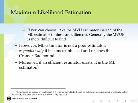
⇒ If you can choose, take the MVU estimator instead of theML estimator (if these are different). Generally the MVUEis more difficult to find.

• However, ML estimator is not a poor estimator:asymptotically it becomes unbiased and reaches theCramer-Rao bound.

• Moreover, if an efficient estimator exists, it is the MLestimator.1

1Remember, an estimator is efficient if it reaches the CRLB. If such an estimator does not exist, we should selectthe MVUE, which in this case is not necessarily the MLE.

Definition

• The Maximum Likelihood estimate for a scalar parameterθ is defined to be the value that maximizes p(x; θ).

• p(x; θ) is the likelihood function and lnp(x; θ) is thelog-likelihood function. Note that it is equivalent tomaximize either of these. Usually the log-likelihood iseasier when the distribution is exponential:

θML = arg maxθ

(p(x; θ))

= arg maxθ

(ln(p(x; θ)))

• In other words, the argument θ that maximizes thefunction p(x; θ) or lnp(x; θ).

Example

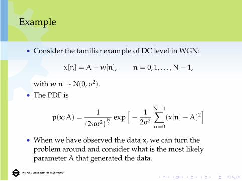
• Consider the familiar example of DC level in WGN:

x[n] = A+w[n], n = 0, 1, . . . ,N− 1,

with w[n] ∼ N(0,σ2).• The PDF is

p(x;A) =1

(2πσ2)N2

exp[−

12σ2

N−1∑n=0

(x[n] −A)2]

• When we have observed the data x, we can turn theproblem around and consider what is the most likelyparameter A that generated the data.

Example

• Some authors emphasize this by turning the order around:p(A; x) or give the function a different name such as L(A; x)or `(A; x).

• So, consider p(x;A) as a function of A and try to maximizeit.

Example

• The picture below shows the likelihood function and thelog-likelihood function for one possible realization of data.The data consists of 50 points, with true A = 5. Thelikelihood function gives the probability of observing theseparticular points with different values of A.

Example

3 3.5 4 4.5 5 5.5 6 6.5 70

0.2

0.4

0.6

0.8

1x 10

−26 The likelihood function

Value of A

Pro

babi

lity

of th

e da

ta

3 3.5 4 4.5 5 5.5 6 6.5 7

−250

−200

−150

−100

−50The log−likelihood function

Value of A

Log

of th

e pr

obab

ility

of t

he d

ata

Example

• Maximization of p(x;A) is not easy in this case, therefore,we take the logarithm, and maximize it instead:

p(x;A) =1

(2πσ2)N2

exp[−

12σ2

N−1∑n=0

(x[n] −A)2]

lnp(x;A) = −N

2ln(2πσ2) −

12σ2

N−1∑n=0

(x[n] −A)2

• The maximum is obtained via differentiation:

∂ lnp(x;A)∂A

=1σ2

N−1∑n=0

(x[n] −A)

Example

• Setting this equal to zero gives

1σ2

N−1∑n=0

(x[n] −A) = 0

N−1∑n=0

(x[n] −A) = 0

N−1∑n=0

x[n] −

N−1∑n=0

A = 0

N−1∑n=0

x[n] −NA = 0

N−1∑n=0

x[n] = NA

A =1N

N−1∑n=0

x[n]

Example

• Thus, A = 1N

∑N−1n=0 x[n] is the ML estimator. Since an

efficient estimator for this problem exists, the ML estimatorreaches it.

Example 2: comparison

• Let us modify the DC level problem such that A is not onlythe DC level, but also the noise variance:

x[n] = A+w[n], n = 0, 1, . . . ,N− 1,

with w[n] ∼ N(0,A).

• Consider three approaches: CRLB factorization, RBLStheorem and ML estimation.


1. CRLB• The CRLB theorem says, that A is the MVU (and efficient)

estimator if we can factor the the first derivative of thelog-likelihood function as follows:

∂ lnp(x;A)∂A

= I(A)(g(x) −A)

• In this case the function becomes

∂ lnp(x;A)∂A

= −N

2A+

1A

N−1∑n=0

(x[n]−A)+1

2A2

N−1∑n=0

(x[n]−A)2

• It seems the this function can not be factored into therequired form, so CRLB can not be used.


• Note: the CRLB can be shown to be

var(A) >A2

N(A+ 12 )

.

2. RBLS• The Rao-Blackwell-Lehmann-Scheffe method first searches

for a sufficient statistic and then transforms it into anunbiased estimator.

• Can we factor the PDF as

p(x;A) = g(T(x), A)h(x)

• Yes:


p(x;A) =1

(2πA)N2

exp

[−

12A

N−1∑n=0

(x[n] −A)2

]

= · · · =1

(2πA)N2

exp

[−

12

(1A

N−1∑n=0

x2[n] +NA

)]︸︷︷︸

g(T(x),A)

exp(Nx)︸︷︷︸h(x)

where T(x) =∑N−1n=0 x

2[n] is the sufficient statistic.• The next step is to transform T(x) unbiased.• The expectation is

E(T(x)) = · · · = N(A+A2)


• It seems that there’s no way to find a function g such that

E(g(T(x))) = A

• The second alternative given by RBLS theorem is notpractical, either, because it requires the calculation of

E(A|T(x)

),

where A is any unbiased estimator of A, e.g., A = x[0].


3. ML• The log-likelihood function and its derivative has been

calculated in the CRLB case:

∂ lnp(x;A)∂A

= −N

2A+

1A

N−1∑n=0

(x[n]−A)+1

2A2

N−1∑n=0

(x[n]−A)2

• Let’s set it to zero to find the ML estimator:

A2 + A−1N

N−1∑n=0

x2[n] = 0.

A = −12±

√√√√ 1N

N−1∑n=0

x2[n] +14


• Of the two alternatives, we discard the negative one,because variance estimate has to be positive:

A = −12+

√√√√ 1N

N−1∑n=0

x2[n] +14

• The estimator is biased since


E(A) = E

(−

12+

√√√√ 1N

N−1∑n=0

x2[n] +14

)

, −12+

√√√√E( 1N

N−1∑n=0

x2[n])+

14

(Expectation does not

carry over sqrt

)

= −12+

√A+A2 +

14

= A.


• In practice the bias is negligible when N is large enough:the figure below shows the variance and the bias of the MLestimator as a function of N. The curves are averages of1000000 realizations.

0 20 40 60 80 100 120 140 160 180 2000

1

2

3

4

5

6

Sample size N

Est

imat

or v

aria

nce

0 20 40 60 80 100 120 140 160 180 200−0.05

−0.04

−0.03

−0.02

−0.01

0

Sample size N

Est

imat

or b

ias


• For reference, the CRLB is plotted on top of the abovefigure in red. The MLE has a variance very close to thebound. Zooming in gives the picture below.

24 24.1 24.2 24.3 24.4 24.5 24.6 24.7 24.8 24.9 252.34

2.36

2.38

2.4

2.42

2.44

2.46

2.48

Sample size N

Est

imat

or v

aria

nce CRLB

Variance of the MLE

• The MLE has actually smaller variance than the theoreticallimit. This is because the limit only applies to unbiasedestimators and ours is biased.

• The bias seems to approach zero as N→∞. This can beshown theoretically:


• By the law of large numbers

1N

N−1∑n=0

x2[n]→ E(x2[n]) = A+A2, when N→∞• Therefore,

A→ A (consistent estimator)

• By linearizing we obtain for large N:

A ≈ A+12

A+ 12

[1N

N−1∑n=0

x2[n] − (A+A2)

].


• And therefore,

E(A) ≈ E

(A+

12

A+ 12

[1N

N−1∑n=0

x2[n] − (A+A2)

])

= A+12

A+ 12

[1N

N−1∑n=0

E(x2[n]) − (A+A2)

]

= A+12

A+ 12

[A+A2 − (A+A2)

]= A+ 0 = A


• Similarly, the linearization gives the asymptotic variance as

var(A) = var

[A+

12

A+ 12

[1N

N−1∑n=0

x2[n] − (A+A2)

]]

=( 1

2

A+ 12

)2var[ 1N

N−1∑n=0

x2[n]]

=14

N(A+ 12 )

2var(x2[n])

=14

N(A+ 12 )

24A2(A+

12)

=A2

N(A+ 12 )


• As we saw earlier, this is the CRLB.• Thus, the ML estimator is asymptotically efficient.• Furthermore, it has a Gaussian pdf.

Summary of properties

• The MLE always becomes optimal and unbiased asN→∞.

• Sometimes the MLE is optimal with finite sample sizes, aswell. More specifically, if an efficient estimator exists(reaching the CRLB), the MLE will be it. If it does not exist,there might be a better alternative than the MLE.

• The asymptotic efficiency and unbiasedness are describedin more exact terms in the following theorem.

Summary of properties

TheoremAsymptotic properties of the MLE: If the pdf p(x; θ) of the data xsatisfies some “regularity” conditions, then the MLE of the unknownparameter θ is asymptotically distributed (for large data records)according to

θa∼ N(θ, I−1(θ)) (1)

where I(θ) is the Fisher information evaluated at the true value of theunknown parameter.The “regularity” conditions require the existence of thederivatives of the log-likelihood function, as well as the Fisherinformation being non-zero.

Example: Sinusoidal parameter estimation

• The main advantage of the MLE is that it is often easy tofind in practical problems.

• Consider the phase estimation problem:

x[n] = A cos(2πf0n+ φ) +w[n],

where A and f0 are known, w[n] ∼ N(0,σ2) and we are toestimate the phase φ.

• The sufficient statistic won’t help us, because there’s nosingle statistic.


• Instead, in Chapter 5, the book shows that the statistics

T1(x) =

N−1∑n=0

x[n] cos(2πf0n)

T2(x) =

N−1∑n=0

x[n] sin(2πf0n)

are jointly sufficient. However, this does not help us infinding the MVU.

• Let’s try the MLE.


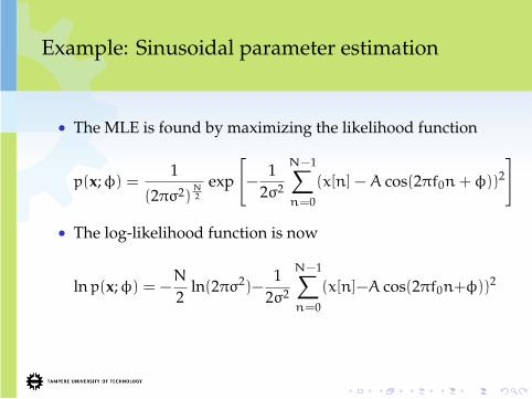
• The MLE is found by maximizing the likelihood function

p(x;φ) =1

(2πσ2)N2

exp

[−

12σ2

N−1∑n=0

(x[n] −A cos(2πf0n+ φ))2

]

• The log-likelihood function is now

lnp(x;φ) = −N

2ln(2πσ2)−

12σ2

N−1∑n=0

(x[n]−A cos(2πf0n+φ))2


• Differentiating it produces

∂ lnp(x;φ)∂φ

=1σ2

N−1∑n=0

(x[n]−A cos(2πf0n+φ))A sin(2πf0n+φ)

• Setting the differential equal to zero gives an equation forthe estimator φ:

A

σ2

N−1∑n=0

x[n] sin(2πf0n+φ)−A

σ2

N−1∑n=0

A cos(2πf0n+φ) sin(2πf0n+φ) = 0


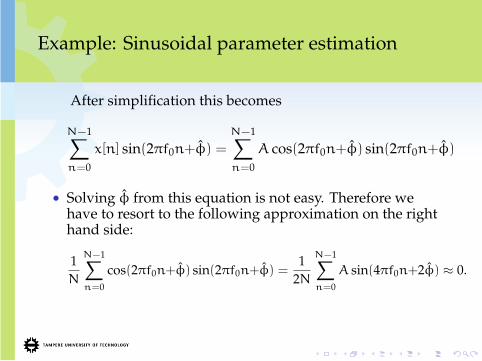
After simplification this becomes

N−1∑n=0

x[n] sin(2πf0n+φ) =

N−1∑n=0

A cos(2πf0n+φ) sin(2πf0n+φ)

• Solving φ from this equation is not easy. Therefore wehave to resort to the following approximation on the righthand side:

1N

N−1∑n=0

cos(2πf0n+φ) sin(2πf0n+φ) =1

2N

N−1∑n=0

A sin(4πf0n+2φ) ≈ 0.


• This means that even after multiplication by N the term onthe right hand side is close to zero. Thus,2

N−1∑n=0

x[n] sin(2πf0n+ φ) ≈ 0

2The effect of this approximation was studied in the mandatory Matlab assignment of the course of 2009. It wasdiscovered that the effect is in fact negligible.


• We can solve φ from here using the triangular equality

sin(α+ β) = cosα sinβ+ sinα cosβ

or in our case:

N−1∑n=0

x[n] sin(2πf0n+ φ)

=

N−1∑n=0

x[n] sin(2πf0n) cos(φ) +N−1∑n=0

x[n] cos(2πf0n) sin(φ) ≈ 0


• Further manipulation gives

sin(φ)N−1∑n=0

x[n] cos(2πf0n) ≈ − cos(φ)N−1∑n=0

x[n] sin(2πf0n)

andsin(φ)cos(φ)

≈ −

∑N−1n=0 x[n] sin(2πf0n)∑N−1n=0 x[n] cos(2πf0n)

• Finally, the approximate ML estimator is

φ ≈ − arctan∑N−1n=0 x[n] sin(2πf0n)∑N−1n=0 x[n] cos(2πf0n)


• A result of a simulated test is shown in the picture below.Blue curve shows the true phase, green circles are the noisydata used for the estimation and red line is the estimationresult. In this test, φ = 0.4, N = 100, A = 1, f0 = 0.14 andσ2 = 5. The estimate φ = 0.12.

0 20 40 60 80 100 120 140 160 180 200−4

−2

0

2

4


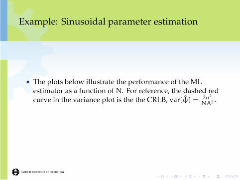
• The plots below illustrate the performance of the MLestimator as a function of N. For reference, the dashed redcurve in the variance plot is the the CRLB, var(φ) = 2σ2

NA2 .


0 20 40 60 80 100 120 140 160 180 2000

0.2

0.4

0.6

0.8

1

Data record length N

Var

ianc

e

0 20 40 60 80 100 120 140 160 180 200−0.25

−0.2

−0.15

−0.1

−0.05

0

0.05

0.1

Data record length N

Bia

s

• The performance of the estimator seems to get reasonablyclose to an unbiased optimal estimator after N > 100.


• The distribution of the estimates is shown in the below plotfor the case N = 30. The true value is 0.4.

−2 −1.5 −1 −0.5 0 0.5 1 1.5 20

200

400

600

800

Phase estimate

MLE of transformed parameters

• Often it is required to estimate a transformed parameterinstead of the one the PDF depends on.

• For example, in the DC-level problem we might beinterested in the power of the signal, A2 instead of themean, A.

• Can we transform the ML estimator of A directly: (A)2?• For example, consider estimation of transformed DC level

in WGN

x[n] = A+w[n], n = 0, 1, . . . ,N− 1

where w[n] is WGN with variance σ2. We wish to find theMLE of a transformed parameter: α = exp(A).


• The PDF is given by

p(x;A) =1

(2πσ2)N2

exp[−

12σ2

N−1∑n=0

(x[n]−A)2]

for −∞ < A <∞• In terms of the transformed parameter α = exp(A), the

PDF becomes

pT (x;α) =1

(2πσ2)N2

exp[−

12σ2

N−1∑n=0

(x[n] − lnα)2]

for α > 0


• Setting the derivative of pT (x;α) with respect to α equal tozero yields:

N−1∑n=0

(x[n] − ln α)1α

= 0 ⇒ α = exp(x)

• Thus, it seems that we can simply transform the estimator.

• Let’s see another example before we state thetransformation theorem.


• Second example: Transformed DC level in WGN withα = A2.

• Now the inverse relation is

A = ±√α

because the transformation is not one-to-one.• If we choose only either

√α or −

√α, then we won’t get all

possible PDF’s. In practise, the estimation would fail if thetrue A would have a different sign than the square root wechose.


• We actually have to consider two pdf’s:

pT1(x;α) =1

(2πσ2)N2

exp[−

12σ2

N−1∑n=0

(x[n]−√α)2]

for α > 0

pT2(x;α) =1

(2πσ2)N2

exp[−

12σ2

N−1∑n=0

(x[n]+√α)2]

for α > 0

• Then we’ll solve the ML estimation problem in both casesand choose the one that has higher maximum value:

α = arg maxα

{pT1(x;α),pT2(x;α)}


• The three likelihood functions are plotted below.

−6 −5 −4 −3 −2 −1 0 1 20

2

4

6

8

x 10−42 The likelihood function

Value of A

Pro

babi

lity

of th

e da

ta

0 2 4 6 8 10 120

0.5

1

1.5

x 10−54 The transformed likelihood function 1 (for positive A)

Value of α

Pro

babi

lity

of th

e da

ta

0 2 4 6 8 10 120

2

4

6

8

x 10−42 The transformed likelihood function 2 (for negative A)

Value of α

Pro

babi

lity

of th

e da

ta

• In a sense, the first likelihood function is searching for apositive A =

√α and the second for negative A = −

√α.


• It is clear that the maximum likelihood estimate for α = A2

is around 3.5 corresponding to A ≈ −1.8. In this examplethe true A = −2.

• It can be shown that the general MLE is α = (A)2 = (x)2.

TheoremInvariance property of the MLE: The MLE of the parameterα = g(θ), where the pdf p(x; θ) is parameterized by θ, is given by

α = g(θ)

where θ is the MLE of θ. The MLE of θ is obtained by maximizingp(x; θ). If g is a not a one-to-one function, then α maximizes themodified likelihood function p(x; θ), defined as

p(x;α) = max{θ:α=g(θ)}

p(x; θ).

Documents

Maximum Likelihood Estimation - TUThehu/SSP/lecture6.pdf · Maximum Likelihood Estimation)If you can choose, take the MVU estimator instead of the ML estimator (if these are di erent)