Maximizing Overall Diversity for Improved Uncertainty Estimates in DeepEnsembles

Siddhartha Jain,*1 Ge Liu,*1 Jonas Mueller,2 David Gifford,1*The authors contribute equally, 1CSAIL,MIT, 2Amazon Web Services

sj1@mit.edu, geliu@mit.edu, jonasmue@amazon.com, gifford@mit.edu

AbstractThe inaccuracy of neural network models on inputs thatdo not stem from the distribution underlying the trainingdata is problematic and at times unrecognized. Uncer-tainty estimates of model predictions are often basedon the variation in predictions produced by a diverseensemble of models applied to the same input. Herewe describe Maximize Overall Diversity (MOD), anapproach to improve ensemble-based uncertainty esti-mates by encouraging larger overall diversity in ensem-ble predictions across all possible inputs. We apply MODto regression tasks including 38 Protein-DNA bindingdatasets, 9 UCI datasets, and the IMDB-Wiki imagedataset. We also explore variants that utilize adversar-ial training techniques and data density estimation. Forout-of-distribution test examples, MOD significantly im-proves predictive performance and uncertainty calibra-tion without sacrificing performance on test data drawnfrom same distribution as the training data. We also findthat in Bayesian optimization tasks, the performanceof UCB acquisition is improved via MOD uncertaintyestimates.

IntroductionModel ensembling provides a simple, yet extremely effec-tive technique for improving the predictive performance ofarbitrary supervised learners each trained with empirical riskminimization (ERM) (Breiman 1996; Brown 2004). Often,ensembles are utilized not only to improve predictions on testexamples stemming from the same underlying distribution asthe training data, but also to provide estimates of model un-certainty when learners are presented with out-of-distribution(OOD) examples that may look different than the data en-countered during training (Lakshminarayanan, Pritzel, andBlundell 2017; Osband et al. 2016). The widespread successof ensembles crucially relies on the variance-reduction pro-duced by aggregating predictions that are statistically prone todifferent types of individual errors (Kuncheva and Whitaker2003). Thus, prediction improvements are best realized byusing a large ensemble with many base models, and a largeensemble is also typically employed to produce stable dis-tributional estimates of model uncertainty (Breiman 1996;Papadopoulos, Edwards, and Murray 2001).

Copyright c© 2020, Association for the Advancement of ArtificialIntelligence (www.aaai.org). All rights reserved.

Practical applications of massive neural networks (NN)are commonly limited to small ensembles because of theunwieldy nature of these models (Osband et al. 2016;Balan et al. 2015; Beluch et al. 2018). Although supervisedlearning performance may be enhanced by an ensemble com-prised of only a few ERM-trained models, the resultingensemble-based uncertainty estimates can exhibit excessivesampling variability in low-density regions of the underlyingtraining distribution. Consider the example of an ensemblecomprised of five models whose predictions just might agreeat points far from the training data by chance. Figure 1 de-picts an example of this phenomenon, which we refer to asuncertainty collapse, since the resulting ensemble-based un-certainty estimates would indicate these predictions are ofhigh-confidence despite not being supported by any nearbytraining datapoints.

Unreliable uncertainty estimates are highly undesirable inapplications where future input queries may not stem fromthe same distribution. A shift in input distribution can becaused by sampling bias, covariate shift, and the adaptiveexperimentation that occurs in bandits, Bayesian optimization(BO), and reinforcement learning (RL) contexts. Here, wepropose Maximize Overall Diversity (MOD), a technique tostabilize OOD model uncertainty estimates produced by anensemble of arbitrary neural networks. The core idea is toconsider all possible inputs and encourage as much overalldiversity in the corresponding model ensemble outputs as canbe tolerated without diminishing the ensemble’s predictiveperformance. MOD utilizes an auxiliary loss function anddata-augmentation strategy that is easily integrated into anyexisting training procedure.

Related WorkNN ensembles have been previously demonstrated to pro-duce useful uncertainty estimates for sequential experimen-tation applications in Bayesian optimization and reinforce-ment learning (Papadopoulos, Edwards, and Murray 2001;Lakshminarayanan, Pritzel, and Blundell 2017; Riquelme,Tucker, and Snoek 2018). Proposed methods to improveensembles include adversarial training to enforce smooth-ness (Lakshminarayanan, Pritzel, and Blundell 2017), andmaximizing ensemble output diversity over the training data(Brown 2004). Recent work has proposed regularizers basedon augmented out-of-distribution examples, but is primar-

arX

iv:1

906.

0738

0v2

[cs

.LG

] 1

2 Fe

b 20

20

ily specific to classification tasks and non-trivially requiresauxiliary generators of OOD examples (Lee et al. 2018) orexisting examples from other classes (Vyas et al. 2018). An-other line of related work solely aims at producing betterout-of-distribution detectors (Liang, Li, and Srikant 2017;Choi and Jang 2018; Ren et al. 2019).

Our work seeks to improve uncertainty estimates in regres-sion settings, where OOD data can stem from an arbitraryunknown distribution, and robust prediction on OOD datais desired rather than just detection of OOD examples. Wepropose a simple technique to regularize ensemble behaviorover all possible inputs that does not require training of ad-ditional generator. Consideration of all possible inputs haspreviously been advocated by (Hooker and Rosset 2012),although not in the context of uncertainty estimation. Pearceet al. (2018) propose a regularizer to ensure an ensembleapproximates a valid Bayesian posterior, but their method-ology is only applicable to homoskedastic noise unlike ours.Hafner et al. (2018) also aim to control Bayesian NN output-behavior beyond the training distribution, but our methodsdo not require the Bayesian formulation they impose andcan be applied to arbitrary NN ensembles, which are oneof the most straightforward methods used for quantifyingNN uncertainty (Papadopoulos, Edwards, and Murray 2001;Lakshminarayanan, Pritzel, and Blundell 2017; Riquelme,Tucker, and Snoek 2018). Malinin and Gales (2018) focuson incorporating distributional uncertainty into uncertaintyestimates via an additional prior distribution, whereas ourfocus is on improving model uncertainty in model ensembles.

MethodsWe consider standard regression, assuming continuous targetvalues are generated via Y = f(X) + ε with ε ∼ N(0, σ2

X),such that σX may heteroscedastically depend on feature val-ues X . Given a limited training dataset D = {xn, yn}Nn=1,where xn ∼ Pin specifies the underlying data distributionfrom which the in-distribution examples in the training dataare sampled, our goal is to learn an ensemble of M neuralnetworks that accurately models both the underlying functionf(x) as well as the uncertainty in ensemble estimates of f(x).Of particular concern are scenarios where test examples xmay stem from a different distribution Pout 6= Pin, which werefer to as out-of-distribution (OOD) examples. As in (Lak-shminarayanan, Pritzel, and Blundell 2017), each networkm (with parameters θm) in our NN ensemble outputs bothan estimated mean µm(x) to predict f(x) and an estimatedvariance σ2

m(x) to predict σ2x, and the per network loss func-

tion L(θm;xn, yn) = − log pθm(yn|xn), is chosen as thenegative log-likelihood (NLL) under the Gaussian assump-tion yn ∼ N(µm(xn), σ

2m(xn)). While traditional bagging

provides different training data to each ensemble member,we simply train each NN using the entire dataset, since therandomness of separate NN-initializations and SGD-trainingsuffice to produce comparable performance to bagging ofNN models (Lakshminarayanan, Pritzel, and Blundell 2017;Lee et al. 2015; Osband et al. 2016).

Following (Lakshminarayanan, Pritzel, and Blundell2017), we estimate PY |X=x (and NLL with respect to

the ensemble) by treating the aggregate ensemble out-put as a single Gaussian distribution N(sµ(x), sσ2(x)).Here, the ensemble-estimate of f(x) is given by sµ(x) =meanp{µm(x)}Mm=1q, and the uncertainty in the target valueis given by sσ2(x) = σ2

eps(x) + σ2mod(x) based on noise-level

estimate σ2eps(x) = meanp{σ2

m(x)}Mm=1q and model uncer-tainty estimate σ2

mod(x) = variancep{µm(x)}Mm=1q. Whilewe focus on Gaussian likelihoods for simplicity, our proposedmethodology is applicable to general parametric conditionaldistributions.

Maximizing Overall Diversity (MOD)Assuming X ∈ X , Y ∈ [−C,C] have been scaled tobounded regions, MOD encourages higher ensemble diver-sity by introducing an auxiliary loss that is computed overaugmented data sampled from another distribution QX . LikePin, QX is also defined over the input feature space, butdiffers from the underlying training data distribution and in-stead describes OOD examples that could be encountered attest-time. The underlying population objective we target is

minθ1,...,θM

Lin − γLout where

Lin =1

M

M∑m=1

EPin[L(θm, x, y)]

Lout = EQ[σ2mod(x)]

(1)

with L as the original supervised learning loss function(e.g. NLL), and a user-specified penalty γ > 0. Since NLLentails a proper-scoring rule (Lakshminarayanan, Pritzel, andBlundell 2017), minimizing the above objective with a suf-ficiently small value of γ will ensure the ensemble seeks torecover PY |X=x for inputs x that lie in the support of thetraining distribution Pin and otherwise output large modeluncertainty for OOD x that lie outside this support. As itis difficult in most applications to specify how future OODexamples may look, we aim to ensure our ensemble outputshigh uncertainty estimates for any possible Pout by taking theentire input space into consideration. To account for any pos-sible OOD distribution, we simply pick QX as the uniformdistribution over X , the bounded region of all possible inputsx. This choice is motivated by Theorem 1 below, which statesthat the uniform distribution most closely approximates allpossible OOD distributions in the minimax sense.

Theorem 1 The uniform distribution QX equals:arg min

Q∈PmaxPout∈P

KL(P ||Q) where for discrete X , Pdenotes the set of all distributions, and for continuous X , Pis the set of all distributions with density functions that arebounded within some interval [a, b].

Proof For the discrete case with |X |= N : let Pout, Qhave corresponding pmf p, q, so KL(Pout||Q) =∑x∈X p(x) log p(x)−

∑x∈X p(x) log q(x). When Q is the

uniform distribution, the worst case Pout is one that putsall its mass on a single point x, which corresponds toKL(Pout||Q) = logN . For any non-uniform Q′: there ex-ists x′ where q′(x′) < q(x′) = 1/N . Thus for P ′

out which

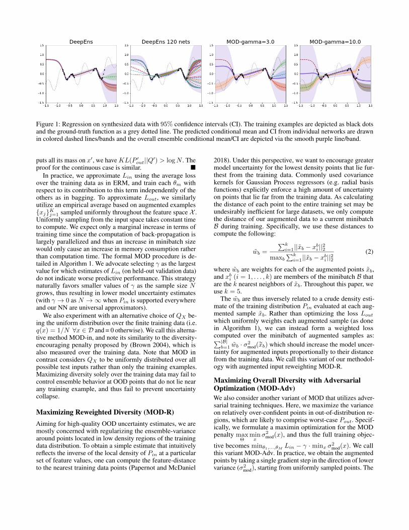
Figure 1: Regression on synthesized data with 95% confidence intervals (CI). The training examples are depicted as black dotsand the ground-truth function as a grey dotted line. The predicted conditional mean and CI from individual networks are drawnin colored dashed lines/bands and the overall ensemble conditional mean/CI are depicted via the smooth purple line/band.

puts all its mass on x′, we have KL(P ′out||Q′) > logN . The

proof for the continuous case is similar. �In practice, we approximate Lin using the average loss

over the training data as in ERM, and train each θm withrespect to its contribution to this term independently of theothers as in bagging. To approximate Lout, we similarlyutilize an empirical average based on augmented examples{xj}Kj=1 sampled uniformly throughout the feature space X .Uniformly sampling from the input space takes constant timeto compute. We expect only a marginal increase in terms oftraining time since the computation of back-propagation islargely parallelized and thus an increase in minibatch sizewould only cause an increase in memory consumption ratherthan computation time. The formal MOD procedure is de-tailed in Algorithm 1. We advocate selecting γ as the largestvalue for which estimates of Lin (on held-out validation data)do not indicate worse predictive performance. This strategynaturally favors smaller values of γ as the sample size Ngrows, thus resulting in lower model uncertainty estimates(with γ → 0 as N →∞ when Pin is supported everywhereand our NN are universal approximators).

We also experiment with an alternative choice of QX be-ing the uniform distribution over the finite training data (i.e.q(x) = 1/N ∀x ∈ D and = 0 otherwise). We call this alterna-tive method MOD-in, and note its similarity to the diversity-encouraging penalty proposed by (Brown 2004), which isalso measured over the training data. Note that MOD incontrast considers QX to be uniformly distributed over allpossible test inputs rather than only the training examples.Maximizing diversity solely over the training data may fail tocontrol ensemble behavior at OOD points that do not lie nearany training example, and thus fail to prevent uncertaintycollapse.

Maximizing Reweighted Diversity (MOD-R)Aiming for high-quality OOD uncertainty estimates, we aremostly concerned with regularizing the ensemble-variancearound points located in low density regions of the trainingdata distribution. To obtain a simple estimate that intuitivelyreflects the inverse of the local density of Pin at a particularset of feature values, one can compute the feature-distanceto the nearest training data points (Papernot and McDaniel

2018). Under this perspective, we want to encourage greatermodel uncertainty for the lowest density points that lie fur-thest from the training data. Commonly used covariancekernels for Gaussian Process regressors (e.g. radial basisfunctions) explicitly enforce a high amount of uncertaintyon points that lie far from the training data. As calculatingthe distance of each point to the entire training set may beundesirably inefficient for large datasets, we only computethe distance of our augmented data to a current minibatchB during training. Specifically, we use these distances tocompute the following:

wb =

∑ki=1||xb − xbi ||22

maxb∑ki=1||xb − xbi ||22

(2)

where wb are weights for each of the augmented points xb,and xbi (i = 1, . . . , k) are members of the minibatch B thatare the k nearest neighbors of xb. Throughout this paper, weuse k = 5.

The wb are thus inversely related to a crude density esti-mate of the training distribution Pin evaluated at each aug-mented sample xb. Rather than optimizing the loss Loutwhich uniformly weights each augmented sample (as donein Algorithm 1), we can instead form a weighted losscomputed over the minibatch of augmented samples as:∑|B|b=1 wb · σ2

mod(rxb) which should increase the model uncer-tainty for augmented inputs proportionally to their distancefrom the training data. We call this variant of our methodol-ogy with augmented input reweighting MOD-R.

Maximizing Overall Diversity with AdversarialOptimization (MOD-Adv)We also consider another variant of MOD that utilizes adver-sarial training techniques. Here, we maximize the varianceon relatively over-confident points in out-of-distribution re-gions, which are likely to comprise worst-case Pout. Specif-ically, we formulate a maximin optimization for the MODpenalty max

Θminxσ2

mod(x), and thus the full training objec-

tive becomes minθ1,...,θM Lin − γ · minx σ2mod(x). We call

this variant MOD-Adv. In practice, we obtain the augmentedpoints by taking a single gradient step in the direction of lowervariance (σ2

mod), starting from uniformly sampled points. The

extra gradient step can double the computation time com-pared to MOD. The full algorithm is given in Algorithm 1.Note that MOD-Adv is different than the traditional adversar-ial training in two aspects: first it takes a gradient step withregard to the model uncertainty measurement (the varianceof ensemble mean prediction) instead of with regard to thepredicted score of another class; second, the adversarial stepis taken starting from a uniformly sampled example insteadof a training example. We apply MOD-Adv to only regres-sion tasks with continuous features since it is more natural toapply gradient descent on them.

Algorithm 1 MOD Training Procedure (+ Variants)Input: Training data D = {(xn, yn)}Nn=1, penalty γ > 0,batch-size |B|Output: Parameters of ensemble of M neural networksθ1,...,θMInitialize θ1,...,θM randomly, initialize wb = 1 for b =1, . . . , |B|repeat

Sample minibatch from training data:{(xb, yb)}|B|b=1

Sample |B| augmented inputs rx1,..., rxB uniformly atrandom from X

if MOD-Adv thenxb ← rxb − αadv · ∇rxb

σ2mod(rxb) ∀1 ≤ b ≤ |B|

for m = 1,. . . , M doif MOD-R then wb = wb (defined in equa-

tion (2))Update θm via SGD with gradient

=1

|B|∇θm

„ |B|∑b=1

L(θm; (xb, yb))− γ|B|∑b=1

wb · σ2mod(rxb)

until iteration limit reached

ExperimentsBaseline MethodsHere, we evaluate various alternative strategies for improv-ing model ensembles. All strategies are applied to the samebase NN ensemble, which is taken to be the Deep Ensem-bles (DeepEns) model of (Lakshminarayanan, Pritzel, andBlundell 2017) previously described in Methods.

Deep Ensembles with Adversarial Training (Deep-Ens+AT) (Lakshminarayanan, Pritzel, and Blundell 2017)used this strategy to improve their basic DeepEns model.The idea is to adversarially sample inputs that lie closeto the training data but on which the NLL loss is high(assuming they share the same label as their neighbor-ing training example). Then, we include these adversar-ial points as augmented data when training the ensemble,which smooths the function learned by the ensemble. Start-ing from training example x, we sample augmented datapointx′ = x+δsign(∇xL(θ, x, y)) with the labels for x′ assumedto be the same as that for the corresponding x. L here denotesthe NLL loss function, and the values for hyperparameter δthat we search over include 0.05, 0.1, 0.2.

Negative Correlation (NegCorr) This method from (Liuand Yao 1999; Shui et al. 2018) minimizes the empiricalcorrelation between predictions of different ensemble mem-bers over the training data. It adds a penalty to the loss ofthe form

∑m[(µm(x) − sµ(x)) ·

∑m′ 6=m(µm′(x) − sµ(x))]

where µm(x) is the prediction of the mth ensemble mem-ber and sµ(x) is the mean ensemble prediction. This penaltyis weighted by a user-specified penalty γ, as done in ourmethodology.

Experiment DetailsAll experiments were run on Nvidia TitanX 1080 Ti andNvidia TitanX 2080 Ti GPUs with PyTorch version 1.0. Un-less otherwise indicated, all p-values were computed usinga single tailed paired t-test per dataset, and the p-values arecombined using Fisher’s method to produce an overall p-value across all datasets in a task. All hyperparameters – in-cluding learning rate, `2-regularization, γ for MOD/NegativeCorrelation, and adversarial training δ – were tuned based onvalidation set NLL. In every regression task, the search forhyperparameter γ was over the values 0.01, 0.1, 1, 5, 10, 20,50. For MOD-Adv, we search for δ over 0.2,1.0,3.0,5.0 forUCI and 0.1,0.5,1 for the image data.

Univariate RegressionWe first consider a one-dimensional regression toy datasetthat is similar to the one used by (Blundell et al. 2015). Wegenerated training data from the function:

y = 0.3x+ 0.3 sin(2πx) + 0.3 sin(4πx) + ε

with ε ∼ N (0, 0.02)

Here, the training data only contain samples drawn from twolimited-size regions. Using the standard NLL loss as well asthe auxiliary MOD penalty, we train a deep ensemble with4 neural networks of identical architectures consisting of 1-hidden layer with 50 units, ReLU activation, two sigmoidoutputs to estimate the mean and variance of PY |X=x, andL2 regularization. To depict the improvement gained by sim-ply adding ensemble members, we also train an ensembleof 120 networks with same architecture. Figure 1 shows thepredictions and 95% confidence interval of the ensembles.MOD is able to produce more reliable uncertainty estimateson the lefthand regions that lack training data, whereas stan-dard deep ensembles exhibit uncertainty collapse, even withmany networks. MOD also properly inflated the predictiveuncertainty in the center region where no training data isfound. Using a smaller γ = 3 in MOD ensures the ensem-ble predictive performance remains strong for in-distributioninputs that lie near the training data and the ensemble ex-hibits adequate levels of certainty around these points. Whilethe larger γ = 10 value leads to overly conservative un-certainty estimates that are large everywhere, we note themean of the ensemble predictions remains highly accuratefor in-distribution inputs.

Protein Binding Microarray DataWe next study scientific data with discrete features by predict-ing Protein-DNA binding. This is a collection of 38 different

microarray datasets, each of which contains measurementsof the binding affinity of a single transcription factor (TF)protein against all possible 8-base DNA sequences (Barreraet al. 2016). We consider each dataset as a separate task withY taken to be the binding affinity scaled to the interval [0,1]and X the one-hot embedded DNA sequence. As we ignorereverse-complements, there are ∼ 32, 000 possible values ofX .

Regression We trained a small ensemble of 4 neural net-works with the same architecture as in the previous experi-ments. We consider 2 different OOD test sets, one comprisedof the sequences with top 10% Y -values and the other com-prised of the sequences with more than 80% of the position inX being G or C (GC-content). For each OOD set, we use theremainder of the sequences as corresponding in-distributionset. We separate them into extremely small training set (300examples) and validation set (300 examples), and use therest as in-distribution test set. We compare MOD along with3 alternative sampling distribution (MOD-in, MOD-R, andMOD-Adv) against the 3 baselines previously mentioned. Wesearch over 0,1e-3,0.01,0.05,0.1 for l2 penalty and 0.01 forlearning rate.

Table 1 and Appendix Table 1 shows mean OOD and in-distribution performance across 38 TFs (averaged over 10runs using random data splits and NN initializations). MODmethods have significantly improved performance on all met-rics and OOD setups compared to DeepEns/DeepEns+AT,both in terms of # of TF outperforming and overall p-valueand is on par with DeepEns+AT on in-Distribution. The re-weighting scheme (MOD-R) further improved the perfor-mance on top 10% Y -value OOD set up. Figure 2 shows thecalibration curve on two of the TFs where the deep ensem-bles are over-confident on top 10% Y -value OOD examples.MOD-R and MOD improve the calibration results by signifi-cant margin compared to most of the baselines.

Bayesian Optimization Next, we compared how theMOD, MOD-R, and MOD-in ensembles performed againstthe DeepEns, DeepEns+AT, and NegCorr ensembles in 38Bayesian optimization tasks using the same protein bindingdata (Hashimoto, Yadlowsky, and Duchi 2018). For eachTF, we performed 30 rounds of DNA-sequence acquisition,acquiring batches of 10 sequences per round in an attemptto maximize binding affinity. We used the upper confidencebound (UCB) as our acquisition function (Chen et al. 2017),ordering the candidate points via sµ(x) + β · σmod(x) (withUCB coefficient β = 1).

At every acquisition iteration, we randomly held out 10%of the training set as the validation set and chose the γ penalty(for MOD, MOD-in, MOD-R, and NegCorr) that producedthe best validation NLL (out of choices: 0, 5, 10, 20, 40,80). The stopping epoch is chosen based on the validationNLL not increasing for 10 epochs with an upper limit of 30epochs. Optimization was done with a learning rate of 0.01,L2 penalty of 0.01 and used the Adam optimizer. For eachof the 38 TFs, we performed 20 Bayesian optimization runswith different seed sequences (same seeds used for all the

Figure 2: Calibration curves for regression models trainedon two of the UCI datasets (top) and two DNA TF bindingdatasets (bottom). A perfect calibration curve should lie onthe diagonal, and an over-confident model has calibrationcurve where the model expected confidence level is higherthan observed confidence level (below diagonal). MOD-Rand MOD significantly improve the over-confident predic-tions from the deep ensembles trained without augmentationloss.

methods) and using 200 points randomly sampled from thebottom 90% of Y values as are initial training set.

We evaluated on the metric of simple regret rT =maxx∈X f(x) −maxt∈[1,T ] f(xt) (second term in the sub-traction quantifies the best point acquired so far and the firstterm is the global best). The results are presented in Table 2.MOD outperforms all other methods in both number of TFswith better regret and the combined p-value. MOD-R is alsostrong outperforming all other methods except MOD withrespect to which is about equivalent in terms of statisticalsignificance. Figure 3 shows rT for the TFs OVOL2 andHESX1, a task in which MOD and MOD-R outperform theother methods.

UCI Regression DatasetsWe next experimented with 9 real world datasets with contin-uous inputs in some applicable bounded domain. We followthe experimental setup that (Lakshminarayanan, Pritzel, andBlundell 2017) and (Hernandez-Lobato et al. 2017) usedto evaluate deep ensembles and deep Bayesian regressors.We split off all datapoints whose y-values fall in the top5% as an OOD test set (so datapoints with such large y-values are never encountered during training). We simulatethe situation where training set is limited and thus used40% of the data for training and 10% for validation. Theremaining data is used as an in-distribution test set. Theanalysis is repeated for 10 random splits of the data toensure robustness. We again use an ensemble of 4 fully-connected neural networks with the same architecture asabove and the NLL training loss searching over hyperparame-

Table 1: NLL on OOD/in-distribution test set averaged across 38 TFs over 10 replicate runs(See Appendix Table 1 for RMSE).MOD out-performance p-value is the combined p-value of MOD NLL being less than the NLL of the method in the correspondingrow. Bold indicates best in category and bold+italicized indicates second best. In case of a tie in the means, the method withlower standard deviation is highlighted.

(MOD out-performance) (MOD out-performance)Methods Out-of-distribution NLL # of TFs p-value In-distribution NLL # of TFs p-value

(OOD as sequences with top 10% binding affinity)DeepEns 0.7485±0.124 26 1.7e-05 -0.4266±0.031 32 7.7e-09DeepEns+AT 0.7438±0.122 25 0.001 -0.4312±0.033 26 0.005NegCorr 0.7358±0.118 27 0.061 -0.4314±0.032 17 0.761MOD 0.7153±0.117 − − -0.4312±0.031 − −MOD-R 0.7225±0.116 22 0.359 -0.4325±0.032 16 0.777MOD-in 0.7326±0.121 26 0.012 -0.4317±0.032 19 0.535

(OOD as sequences with >80% GC content)DeepEns -0.6938±0.052 20 0.022 -0.5649±0.029 34 3.1e-11DeepEns+AT -0.7010±0.041 23 0.007 -0.5740±0.027 21 0.292NegCorr -0.6805±0.065 25 0.011 -0.5700±0.026 25 0.017MOD -0.7007±0.047 − − -0.5729±0.027 − −MOD-R -0.6959±0.040 24 0.004 -0.5720±0.027 22 0.357MOD-in -0.6948±0.054 21 0.103 -0.5711±0.028 22 0.163

Figure 3: Regret for two Bayesian optimization tasks (aver-aged over 20 replicate runs). The bands depict 50% confi-dence intervals, and the x-axis indicates the number of DNAsequences whose binding affinity has been profiled so far.

ter values: L2 penalty ∈ {0, 0.001, 0.01, 0.05, 0.1}, learningrate ∈ {0.0005, 0.001, 0.01}. We report the negative log-likelihood (NLL) on both in- and out-of-distribution testsets for ensembles trained via different strategies (including

Table 2: Regret (rT ) comparison. Each cell shows the numberof TFs (out of 38) for which the method in corresponding rowoutperforms the method in the corresponding column (lowerrT ). The number in parentheses is the combined (across 38TFs) p-value of MOD/-in/-R regret being less than the regretof the method in the corresponding column.

vs DeepEns DeepEns+AT NegCorr

MOD-in 21 (0.111) 21 (0.041) 19 (0.356)MOD 26 (0.003) 24 (0.004) 20 (0.001)MOD-R 22 (0.019) 23 (0.007) 22 (0.017)vs MOD-in MOD MOD-R

MOD-in − 17 (0.791) 16 (0.51)MOD 19 (0.002) − 22 (0.173)MOD-R 20 (0.052) 14 (0.674) −

MOD-Adv) and examine the calibration curves.As shown in Table 3, MOD outperforms DeepEns in 6 out

of the 9 datasets on OOD NLL, and has significant overallp-value compared to all baselines. MOD-Adv ranks top 1in OOD NLL in terms of averaged ranks across all datasets,showing better robustness than MOD. The MOD loss lead tohigher-quality uncertainties on OOD data while also improv-ing in-distribution performance of DeepEns.

Figure 2 shows the calibration curve on two of the datasetswhere the basic deep ensembles exhibit over-confidence onOOD data. Note that retaining accurate calibration on OODdata is extremely difficult for most machine learning meth-ods. MOD and MOD-R improve calibration by a significantmargin compared to most of the baselines, validating theeffectiveness of our MOD procedure.

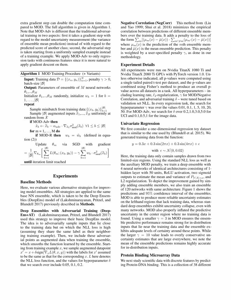
The selection of γ is critical for MOD, thus we also ex-amine the effect of the choice of γ on the in-distributionperformance for the 9 UCI and 38 TF binding regression

Table 3: Averaged NLL on out-of-distribution/in-distribution test example over 10 replicate runs for UCI datasets, top 5%samples were heldout as OOD test set (See Appendix Table 2 for RMSE). MOD outperformance p-value is the combined (viaFisher’s method) p-value of MOD NLL being less than the NLL of the method in the corresponding column (with p-value perdataset being computed using a paired single tailed t-test). Bold indicates best in category and bold+italicized indicates secondbest. In case of a tie in the means, the method with the lower standard deviation is highlighted.

Datasets DeepEns DeepEns+AT NegCorr MOD MOD-R MOD-in MOD-Adv

Out-of-distribution NLLconcrete -0.831±0.237 -0.915±0.204 -0.913±0.277 -0.904±0.118 -0.910±0.193 -0.924±0.188 -0.950±0.200yacht -1.597±0.840 -1.762±0.647 -1.972±0.570 -1.797±0.437 -1.761±0.578 -1.638±0.663 -1.948±0.343naval-propulsion-plant -2.580±0.103 -1.380±0.087 -2.618±0.056 -2.729±0.071 -2.130±0.069 -2.057±0.055 -2.629±0.068wine-quality-red 0.133±0.132 0.115±0.086 0.113±0.104 0.153±0.107 0.084±0.072 0.085±0.065 0.217±0.114power-plant -1.734±0.054 -1.731±0.088 -1.659±0.075 -1.638±0.151 -1.644±0.120 -1.731±0.050 -1.669±0.066protein-tertiary-structure 1.162±0.231 1.178±0.158 1.231±0.130 1.197±0.137 1.194±0.214 1.154±0.132 1.299±0.252kin8nm -1.980±0.053 -1.970±0.093 -2.036±0.046 -1.999±0.049 -2.003±0.095 -1.993±0.078 -2.027±0.085bostonHousing 1.591±0.680 1.243±0.690 1.821±0.913 0.568±0.959 0.460±0.648 0.923±0.733 1.517±0.711energy -1.590±0.253 -1.784±0.153 -1.718±0.193 -1.736±0.117 -1.741±0.264 -1.733±0.199 -1.772±0.242MOD outperformance p-value 0.002 4.9e-07 0.034 - 1.6e-04 4.6e-05 0.027

In-distribution NLLconcrete -1.075±0.094 -1.129±0.084 -1.089±0.102 -1.155±0.086 -1.137±0.132 -1.090±0.092 -1.047±0.177yacht -3.286±0.692 -3.245±0.822 -3.570±0.166 -3.500±0.190 -3.461±0.252 -3.339±0.815 -3.556±0.203naval-propulsion-plant -2.735±0.077 -1.513±0.042 -2.810±0.042 -2.857±0.067 -2.297±0.061 -2.238±0.047 -2.817±0.046wine-quality-red -0.070±0.853 -0.341±0.068 -0.266±0.291 -0.337±0.069 -0.348±0.045 -0.351±0.055 -0.170±0.505power-plant -1.521±0.015 -1.525±0.018 -1.524±0.023 -1.523±0.012 -1.522±0.017 -1.524±0.013 -1.523±0.016protein-tertiary-structure -0.514±0.013 -0.519±0.007 -0.544±0.012 -0.533±0.009 -0.532±0.012 -0.529±0.008 -0.540±0.012kin8nm -1.305±0.016 -1.315±0.020 -1.334±0.015 -1.317±0.019 -1.315±0.017 -1.322±0.015 -1.314±0.020bostonHousing -0.901±0.154 -0.937±0.144 -0.656±0.671 -0.953±0.147 -0.883±0.188 -0.925±0.180 -0.728±0.376energy -2.426±0.151 -2.517±0.098 -2.620±0.130 -2.507±0.153 -2.525±0.098 -2.522±0.129 -2.638±0.137MOD outperformance p-value 2.4e-08 6.9e-11 0.116 - 8.9e-06 2.2e-06 0.046

tasks. As shown in Figure 4, γ generally does not affect orhurt in-distribution NLL until it gets too large at which pointit fairly consistently starts hurting it. When γ is selected prop-erly it may even improve the in-distribution slightly as shownin the previous tables.

Figure 4: The effect of different γ on in-distribution testperformance (NLL).

Age Prediction from ImagesTo demonstrate the effectiveness of MOD, MOD-Adv, andMOD-R on high dimensional data, we consider supervisedlearning with image data. Here, we use a dataset of hu-man images collected from IMDB and Wikimedia and anno-tated with age and gender information (Rothe, Timofte, andVan Gool 2015). The IMDB/Wiki parts of the dataset consistof 460K+/62K+ images respectively. 28,601 images in theWiki dataset are males and the rest are females.

In the context of Wiki images, we tried to predict the agesgiven the image of a person using 2000 images of males asthe training set. For the OOD dataset, we hold out the oldest10% of the people as the OOD set. We used the Wide Resid-ual Network architecture (Zagoruyko and Komodakis 2016)with a depth of 4 and a width factor of 2. As before, we usedan ensemble of size 4. The search for the optimal γ valuewas over 0, 2, 5, 10, 20, 40, 80. The stopping epoch is chosenbased on the validation NLL not increasing for 10 epochswith an upper limit of 30 epochs. Optimization was donewith a learning rate of 0.001, l2 penalty of 0.001 and used theAdam optimizer. The NLL results are in Table 4 whereas theRMSE results are in the Appendix. Both Maximize OverallDiversity and MOD-Adv get the best results on OOD NLLwith the improvement being statistically significant over theother methods. MOD gets an NLL of 1.129 on OOD data,MOD-Adv gets an NLL of 1.155 on OOD, and MOD-R gets1.185 on OOD. This is in contrast to DeepEns which getsonly 1.304 on OOD. Thus both MOD and MOD-R show sig-nificant improvements on NLL on the OOD data. In addition,while DeepEns+AT has a better mean in-distribution NLLcompared to MOD, the focus of this paper is out of distribu-tion uncertainty on which Maximize Overall Diversity andMOD-Adv perform very well. Notably every MOD variantimproves performance for both in and out of distribution.Thus augmenting the loss function with the MOD penaltyshould not make your model worse.

Table 4: Image regression results showing mean performanceacross 20 randomly seeded runs (along with ± one standarddeviation). In-Dist refers to the in-distribution test set. OODrefers to the out of distribution test set. Bold indicates best incategory and bold+italicized indicates second best. In caseof a tie in means, the lower standard deviation method ishighlighted.

Methods OOD NLL In-Dist NLL

DeepEns 1.3100 ± 0.2486 -0.2193 ± 0.0207DeepEns+AT 1.2348±0.1291 -0.2419±0.0213NegCorr 1.1731±0.1978 -0.2286±0.0179MOD-in 1.2625±0.1961 -0.2301±0.0128MOD 1.1294±0.1707 -0.2306±0.0148MOD-R 1.1847±0.2442 -0.2285±0.0191MOD-Adv 1.1547±0.1865 -0.2305±0.0149

ConclusionWe have introduced a loss function and data augmentationstrategy that helps stabilize distribution uncertainty estimatesobtained from model ensembling. Our method increasesmodel uncertainty over the entire input space while simul-taneously maintaining predictive performance, which helpsmitigate uncertainty collapse that may arise in small modelensembles. We further proposed two variants of our method.MOD-R assesses the distance of an augmented sample fromthe training distribution and aims to ensure higher modeluncertainty in regions with low-density, and MOD-Adv usesadversarial optimization to improve model uncertainty on rel-atively over-confident regions more efficiently. Our methodsproduce improvements to both the in and out of distributionNLL, out of distribution RMSE, and calibration on a varietyof datasets drawn from biology, vision, and common UCIdatasets. We also showed MOD is useful in hard Bayesianoptimization tasks. Future work could develop techniquesto generate OOD augmented samples for structured data,as well as applying ensembles with improved uncertainty-awareness to currently challenging tasks such as explorationin reinforcement learning.

References[Balan et al. 2015] Balan, A. K.; Rathod, V.; Murphy, K. P.;and Welling, M. 2015. Bayesian dark knowledge. In Ad-vances in Neural Information Processing Systems.

[Barrera et al. 2016] Barrera, L. A.; Vedenko, A.; Kurland,J. V.; Rogers, J. M.; Gisselbrecht, S. S.; Rossin, E. J.;Woodard, J.; Mariani, L.; Kock, K. H.; Inukai, S.; et al. 2016.Survey of variation in human transcription factors revealsprevalent DNA binding changes. Science 351(6280):1450–1454.

[Beluch et al. 2018] Beluch, W. H.; Genewein, T.;Nurnberger, A.; and Kohler, J. M. 2018. The powerof ensembles for active learning in image classification.In IEEE Conference on Computer Vision and PatternRecognition.

[Blundell et al. 2015] Blundell, C.; Cornebise, J.;

Kavukcuoglu, K.; and Wierstra, D. 2015. Weight uncertaintyin neural networks. arXiv preprint arXiv:1505.05424.

[Breiman 1996] Breiman, L. 1996. Bagging predictors. Ma-chine Learning 24:123–140.

[Brown 2004] Brown, G. 2004. Diversity in neural networkensembles. Ph.D. Dissertation, University of Birmingham.

[Chen et al. 2017] Chen, R. Y.; Sidor, S.; Abbeel, P.; andSchulman, J. 2017. UCB exploration via Q-ensembles.arXiv:1706.01502.

[Choi and Jang 2018] Choi, H., and Jang, E. 2018. Genera-tive ensembles for robust anomaly detection. arXiv preprintarXiv:1810.01392.

[Hafner et al. 2018] Hafner, D.; Tran, D.; Lillicrap, T.; Ir-pan, A.; and Davidson, J. 2018. Reliable uncertainty esti-mates in deep neural networks using noise contrastive priors.arXiv:1807.09289.

[Hashimoto, Yadlowsky, and Duchi 2018] Hashimoto, T. B.;Yadlowsky, S.; and Duchi, J. C. 2018. Derivative free opti-mization via repeated classification. In International Confer-ence on Artificial Intelligence and Statistics.

[Hernandez-Lobato et al. 2017] Hernandez-Lobato, J. M.;Requeima, J.; Pyzer-Knapp, E. O.; and Aspuru-Guzik,A. 2017. Parallel and distributed thompson samplingfor large-scale accelerated exploration of chemical space.arXiv:1706.01825.

[Hooker and Rosset 2012] Hooker, G., and Rosset, S. 2012.Prediction-focused regularization using data-augmented re-gression. Statistics and Computing 1:237–349.

[Kuncheva and Whitaker 2003] Kuncheva, L. I., andWhitaker, C. J. 2003. Measures of diversity in classifierensembles and their relationship with the ensemble accuracy.Machine Learning 51:181–207.

[Lakshminarayanan, Pritzel, and Blundell 2017]Lakshminarayanan, B.; Pritzel, A.; and Blundell, C.2017. Simple and scalable predictive uncertainty estimationusing deep ensembles. In Advances in Neural InformationProcessing Systems.

[Lee et al. 2015] Lee, S.; Purushwalkam, S.; Cogswell, M.;Crandall, D.; and Batra, D. 2015. Why M heads are betterthan one: Training a diverse ensemble of deep networks.arXiv:1511.06314.

[Lee et al. 2018] Lee, K.; Lee, H.; Lee, K.; and Shin, J. 2018.Training confidence-calibrated classifiers for detecting out-of-distribution samples. In International Conference on Learn-ing Representations.

[Liang, Li, and Srikant 2017] Liang, S.; Li, Y.; and Srikant,R. 2017. Enhancing the reliability of out-of-distributionimage detection in neural networks. arXiv preprintarXiv:1706.02690.

[Liu and Yao 1999] Liu, Y., and Yao, X. 1999. Ensem-ble learning via negative correlation. Neural networks12(10):1399–1404.

[Malinin and Gales 2018] Malinin, A., and Gales, M. 2018.Predictive uncertainty estimation via prior networks. InAdvances in Neural Information Processing Systems, 7047–7058.

[Osband et al. 2016] Osband, I.; Blundell, C.; Pritzel, A.; andVan Roy, B. 2016. Deep exploration via bootstrapped DQN.In Advances in Neural Information Processing Systems.

[Papadopoulos, Edwards, and Murray 2001] Papadopoulos,G.; Edwards, P. J.; and Murray, A. F. 2001. Confidence esti-mation methods for neural networks: A practical comparison.IEEE Transactions on Neural Networks 12:1278–1287.

[Papernot and McDaniel 2018] Papernot, N., and McDaniel,P. 2018. Deep k-nearest neighbors: Towards confident,interpretable and robust deep learning. arXiv preprintarXiv:1803.04765.

[Pearce et al. 2018] Pearce, T.; Zaki, M.; Brintrup, A.; andNeel, A. 2018. Uncertainty in neural networks: Bayesianensembling. arXiv preprint arXiv:1810.05546.

[Ren et al. 2019] Ren, J.; Liu, P. J.; Fertig, E.; Snoek, J.;Poplin, R.; DePristo, M. A.; Dillon, J. V.; and Lakshmi-narayanan, B. 2019. Likelihood ratios for out-of-distributiondetection. arXiv preprint arXiv:1906.02845.

[Riquelme, Tucker, and Snoek 2018] Riquelme, C.; Tucker,G.; and Snoek, J. 2018. Deep bayesian bandits showdown:An empirical comparison of bayesian deep networks forthompson sampling. In International Conference on Learn-ing Representations.

[Rothe, Timofte, and Van Gool 2015] Rothe, R.; Timofte, R.;and Van Gool, L. 2015. Dex: Deep expectation of appar-ent age from a single image. In Proceedings of the IEEEInternational Conference on Computer Vision Workshops,10–15.

[Shui et al. 2018] Shui, C.; Mozafari, A. S.; Marek, J.; Hedhli,I.; and Gagne, C. 2018. Diversity regularization in deepensembles. arXiv:1802.07881.

[Vyas et al. 2018] Vyas, A.; Jammalamadaka, N.; Zhu, X.;Das, D.; Kaul, B.; and Willke, T. L. 2018. Out-of-distributiondetection using an ensemble of self supervised leave-outclassifiers. In Proceedings of the European Conference onComputer Vision (ECCV), 550–564.

[Zagoruyko and Komodakis 2016] Zagoruyko, S., and Ko-modakis, N. 2016. Wide residual networks. arXiv preprintarXiv:1605.07146.

Appendix

Table 5: RMSE on OOD/in-distribution test set averaged across 38 TFs over 10 replicate runs. MOD out-performance p-value isthe combined p-value of MOD RMSE being less than the RMSE of the method in the corresponding row. Bold indicates best incategory and bold+italicized indicates second best. In case of a tie in the means, the method with lower standard deviation ishighlighted.

(MOD out-performance) (MOD out-performance)Methods Out-of-distribution RMSE # of TFs p-value In-distribution RMSE # of TFs p-value

(OOD as sequences with top 10% binding affinity)DeepEns 0.2837±0.011 26 1.3e-04 0.1591±0.005 34 2.1e-12DeepEns+AT 0.2812±0.011 23 0.087 0.1582±0.005 28 3.6e-05NegCorr 0.2814±0.010 20 0.124 0.1583±0.005 20 0.492MOD 0.2802±0.010 0 0.0e+00 0.1581±0.005 0 0.0e+00MOD-R 0.2795±0.010 17 0.933 0.1579±0.005 13 0.969MOD-in 0.2801±0.010 16 0.617 0.1581±0.005 18 0.633

(OOD as sequences with >80% GC content)DeepEns 0.1190±0.004 25 0.008 0.1415±0.003 36 8.5e-24DeepEns+AT 0.1180±0.003 19 0.029 0.1394±0.003 22 0.106NegCorr 0.1179±0.004 21 0.052 0.1403±0.003 30 4.7e-08MOD 0.1173±0.003 0 0.0e+00 0.1394±0.003 0 0.0e+00MOD-R 0.1177±0.003 22 0.112 0.1398±0.003 19 0.079MOD-in 0.1177±0.004 21 0.401 0.1403±0.003 27 2.8e-06

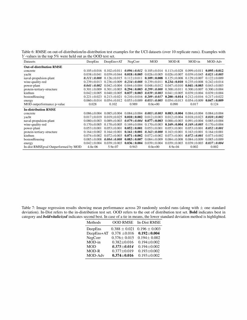
Table 6: RMSE on out-of-distribution/in-distribution test examples for the UCI datasets (over 10 replicate runs). Examples withY -values in the top 5% were held out as the OOD test set.

Datasets DeepEns DeepEns+AT NegCorr MOD MOD-R MOD-in MOD-Adv

Out-of-distribution RMSEconcrete 0.105±0.016 0.102±0.011 0.096±0.012 0.105±0.014 0.113±0.028 0.099±0.011 0.095±0.012yacht 0.038±0.041 0.039±0.044 0.018±0.005 0.026±0.005 0.026±0.007 0.039±0.045 0.021±0.005naval-propulsion-plant 0.111±0.008 0.126±0.015 0.112±0.011 0.109±0.008 0.125±0.008 0.129±0.007 0.122±0.009wine-quality-red 0.239±0.013 0.236±0.009 0.234±0.008 0.239±0.011 0.234±0.010 0.235±0.008 0.242±0.014power-plant 0.041±0.002 0.042±0.004 0.044±0.004 0.048±0.012 0.047±0.010 0.041±0.003 0.043±0.003protein-tertiary-structure 0.301±0.009 0.301±0.003 0.294±0.003 0.299±0.008 0.300±0.011 0.300±0.007 0.300±0.004kin8nm 0.042±0.005 0.040±0.005 0.037±0.003 0.039±0.003 0.041±0.005 0.039±0.004 0.039±0.004bostonHousing 0.221±0.023 0.213±0.021 0.210±0.016 0.209±0.017 0.200±0.014 0.212±0.016 0.217±0.022energy 0.060±0.014 0.054±0.012 0.053±0.009 0.053±0.005 0.054±0.013 0.054±0.009 0.047±0.009MOD outperformance p-value 0.028 0.102 0.989 0.0e+00 0.090 0.017 0.124

In-distribution RMSEconcrete 0.086±0.004 0.085±0.004 0.084±0.004 0.083±0.003 0.083±0.004 0.084±0.004 0.084±0.004yacht 0.017±0.019 0.019±0.025 0.010±0.002 0.012±0.003 0.012±0.004 0.018±0.023 0.010±0.002naval-propulsion-plant 0.080±0.003 0.089±0.003 0.079±0.004 0.077±0.003 0.088±0.003 0.091±0.004 0.085±0.004wine-quality-red 0.170±0.005 0.170±0.005 0.169±0.004 0.170±0.003 0.169±0.004 0.169±0.005 0.170±0.004power-plant 0.053±0.001 0.053±0.001 0.052±0.001 0.053±0.001 0.053±0.001 0.053±0.001 0.052±0.001protein-tertiary-structure 0.164±0.002 0.164±0.001 0.161±0.001 0.163±0.000 0.163±0.001 0.163±0.001 0.164±0.001kin8nm 0.074±0.002 0.072±0.003 0.071±0.002 0.072±0.002 0.073±0.001 0.072±0.001 0.073±0.002bostonHousing 0.085±0.008 0.084±0.008 0.083±0.007 0.084±0.009 0.084±0.008 0.084±0.009 0.085±0.009energy 0.042±0.004 0.039±0.003 0.036±0.004 0.039±0.004 0.039±0.003 0.039±0.003 0.037±0.004In-dist RMSEpval Outperformed by MOD 4.0e-06 5.9e-07 0.943 0.0e+00 8.9e-04 0.002 0.002

Table 7: Image regression results showing mean performance across 20 randomly seeded runs (along with ± one standarddeviation). In-Dist refers to the in-distribution test set. OOD refers to the out of distribution test set. Bold indicates best incategory and bold+italicized indicates second best. In case of a tie in means, the lower standard deviation method is highlighted.

Methods OOD RMSE In-Dist RMSE

DeepEns 0.388 ± 0.021 0.196 ± 0.003DeepEns+AT 0.378 ±0.016 0.192±0.004NegCorr 0.376± 0.015 0.194± 0.002MOD-in 0.382±0.016 0.194±0.002MOD 0.375±0.014 0.194±0.002MOD-R 0.377±0.019 0.193±0.002MOD-Adv 0.374±0.016 0.193±0.002