MAVRIC: Modeling Analysis, Verification, Regulatory and

International Compliance

Modeling to Support Policy Analysis

Modeling Analysis, Verification, Regulatory and International Comparisons

What do energy-economic-environmental models and cross-comparison of models tell us about the future of energy system that include

transportation? Key Research Questions:

• What do existing models at the California, U.S. and international levels tell us about different possible energy and transportation futures and the paths to those futures?

• How have the forecasts and models of market adoption of new vehicle and fuel technologies developed during the STEPS 2007–2010 and NextSTEPS 2011–2014 programs performed relative to their actual market penetration? What lessons can be learned and applied to improve our future models and forecasts?

• How do model projections and scenarios compare and what can we learn from each?

• How can a wide range of diverse and divergent scenarios/modeling outcomes be used to help inform decision-making and policy design in the face of significant uncertainty? Are there robust strategies that we can identify?

• What assumptions are being made and which ones matter most? What metrics of change over time are required to assess the comparative likelihood of alternative energy pathways, including one dominated by shale oil and gas, meeting sustainability goals and timelines?

• How can we improve our own scenario making and use our own models in a better fashion to help us assess policies?

2

STEPS 2015 Projects: MAVRIC - Modeling, Analysis, Verification, and Regional and International Comparisons

3

Models • California

– CA-TIMES: Energy System Model for California • Global

– GCAM: Global Change Assessment Model – MoMo: Global Transport Energy Model (IEA) – Global Oil Model and Global Gas Model

• Transition model – GBSM: Geospatial Biorefinery Siting – Natural Gas Infrastructure model – Hydrogen station siting and rollout models – EV charger siting & rollout models – CCS system model – COCHIN-TIMES (COnsumer CHoice INtegration in TIMES)

• Environment and sustainability – LEM: Life cycle emissions models – AVCEM: Advanced Vehicle Cost & Energy Use Model – Water, land, materials & energy modeling

• Modeling Comparison – CCPM: CA Climate Policy Modeling dialogue project (December 2013, March 2015) – iTEM: International Transport/Energy Model Comparison Project (December 2014)

4

Highlights

• Climate policies in California and the role of academic modeling efforts in supporting policy analysis – California Climate Policy Modeling Dialogue – California energy system model: CA-TIMES – Adapting Consumer Choice Modeling to analyze non-regulatory

policies

• Uncertainty Analysis and Robust Decision Making

5

Since 2007, California gov has started a series of legislations/regulations to mitigation GHG emissions

6

0

100

200

300

400

500

600

700

2000 2010 2020 2030 2040 2050

MM

T CO

2e/y

r

431 MMT CO2e/yr

86 MMT COe/yr

• If we have any chance at all of achieving reductions needed to limit global warming to 2 degrees by 2050 “California must show the way”

• 2030 goals – Increase to 50% electricity

derived from electricity – Reduce petroleum use in

cars & trucks by up to 50% – Double energy efficiency

achieved at existing buildings & make heat fuels cleaner

Governor’s 2030 Climate Goals

Source: CCPM (March 2015)

Business As Usual (BAU) Scenarios CCPM1 (December 2013)

9

80 in '50AB32 Target

Historic

0

200

400

600

800

2000 2010 2020 2030 2040 2050

Annu

al G

HG E

miss

ions

(MM

T CO

2e/y

r)

Historic ARB Scoping Plan, 2008

CCST BEAR

PATHWAYS LEAP/SWITCH

CA-TIMES CALGAPS80% ReductionARB Scoping Plan, 2014

All Models in CCPM2 (2015)

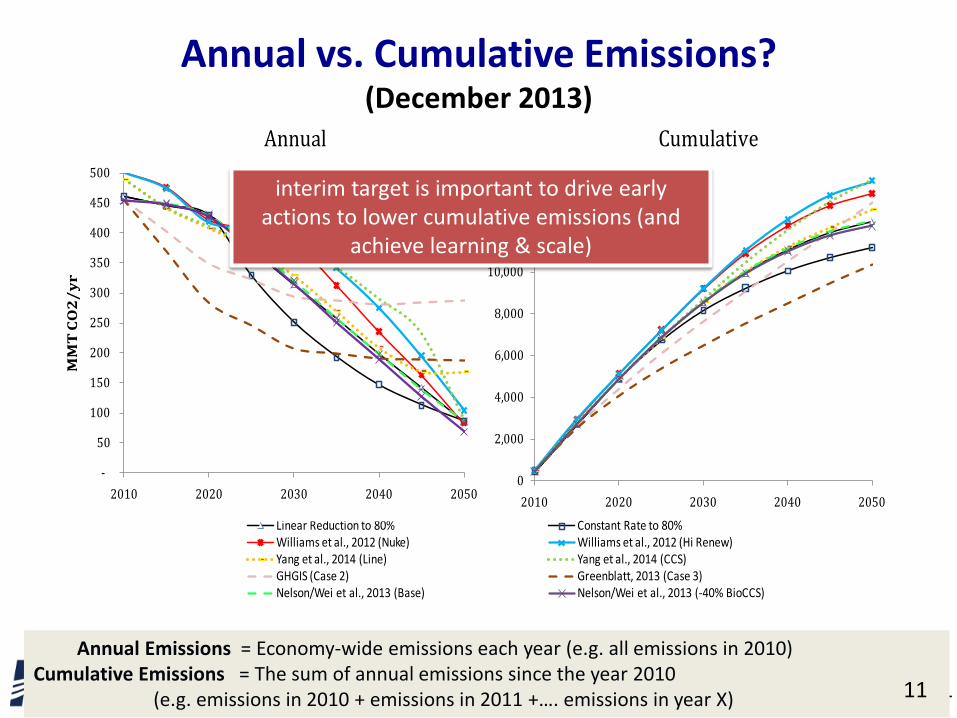
Annual vs. Cumulative Emissions? (December 2013)

12/21

0

2,000

4,000

6,000

8,000

10,000

12,000

14,000

2010 2020 2030 2040 2050

MM

T C

O2

Linear Reduction to 80% Constant Rate to 80%Williams et al., 2012 (Nuke) Williams et al., 2012 (Hi Renew)Yang et al., 2014 (Line) Yang et al., 2014 (CCS)GHGIS (Case 2) Greenblatt, 2013 (Case 3)Nelson/Wei et al., 2013 (Base) Nelson/Wei et al., 2013 (-40% BioCCS)

-

50

100

150

200

250

300

350

400

450

500

2010 2020 2030 2040 2050

MM

T C

O2

/yr

Annual Cumulative

Annual Emissions = Economy-wide emissions each year (e.g. all emissions in 2010) Cumulative Emissions = The sum of annual emissions since the year 2010 (e.g. emissions in 2010 + emissions in 2011 +…. emissions in year X) 11

interim target is important to drive early actions to lower cumulative emissions (and

achieve learning & scale)

Observations from first CCPM forum (December 2013)

• Future modeling efforts should focus on the: – economic impacts and logistical feasibility of given scenarios, – interactive effects between two or more climate policies, – role of uncertainty in the state’s long-term energy planning, and – identification of pathways that achieve the dual goals of criteria

pollutant and GHG emission reduction. • Modelers need to work with policy makers more closely to represent the

details of the policy design • Data availability and data/model transparency is absolutely essential. • Identifying ways to make the models and model findings more useful and

accessible to policy-makers and stakeholders.

5

Key Observations: CCPM2 (March 2015)

• More models show cost impacts: $/HH, $/kWh • More discussion about jobs and heterogeneity of impacts • Forks in the road: Studies illustrate major paradigm shifts necessary for

2050 goals – Massive expansion of biogas production/use – OR large scale electrification of vehicles as well as industrial and home heat

usages – Each fork will eventually requires irreversible investments by someone.

• Are these really forks at the state policy level? – Individuals must choose, but don’t all have to make same choice – Can’t there be a mix of electric heating and biogas?

INDUSTRIES WANT MAXIMUM FLEXIBILITY!

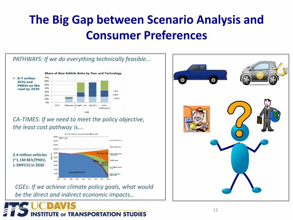
The Big Gap between Scenario Analysis and Consumer Preferences

12

PATHWAYS: If we do everything technically feasible…

CA-TIMES: If we need to meet the policy objective, the least cost pathway is….

2.4 million vehicles (~1.1M BEV/PHEV, 1.3MFCV) in 2030

CGEs: If we achieve climate policy goals, what would be the direct and indirect economic impacts…

Overview of Model Approach

13

• Energy Systems Models – Technology rich on the supply side, but lack behavioral details

• Consumer Choice Models – Detail choices on the demand side but lack supply sector details

• Our focus: ‘Marrying’ these two types of models

Supply-rich COCHIN-TIMES Demand-rich

Minimal Supply rep.

Consumer Choice Model Demand-rich

Supply rich TIMES model Minimal behavior rep.

+

=

COCHIN: COnsumer CHoice INtegration

• System-engineering models typically assume society is homogenous, i.e. there is only one decision-maker at the societal level

• Consumer behavior cannot be ignored in system-wide modeling!

• One objective of this project is to develop a bridging approach to bring in consumer behavioral parameters, to the linear programming framework of TIMES

Motivation for Consumer Choice

14

Need for Consumer Choice in Policy Analysis

Vehicle Price Fuel Cost Perception Infrastructure support

Monetary Costs Disutility Costs

Vehicle Purchase

Consumer Choice

Consumers make decisions based on monetary costs, such as vehicle price, fuel cost, as well as the ‘disutility’ costs, such as their perception of a technology on various issues, and the infrastructure support available.

15

-10000

0

10000

20000

30000

40000

50000

60000

70000

80000

Gasoline Diesel Hybrid Plug-inHybrid

Fuel Cell Electric

$/ve

hicl

e

Model Availability

Risk Premium

Refueling

Charge Refueler Cost

Towing

Range Anxiety Cost

Urban

Early Adopter

Moderate driver

-10000

0

10000

20000

30000

40000

50000

60000

70000

80000

Gasoline Diesel Hybrid Plug-inHybrid

Fuel Cell Electric

$/ve

hicl

e

Model Availability

Risk Premium

Refueling

Charge Refueler Cost

Towing

Range Anxiety Cost

Components of Disutility Cost in the year 2020

Rural

Late Majority

Frequent driver

Range Anxiety Cost

Refueling Inconvenience Cost

Model Availability Cost

Risk Premium

Charger Refueler Cost

Towing Cost

Range Anxiety Cost

Refueling Inconvenience Cost

Model Availability Cost

Risk Premium

Charger Refueler Cost

Towing Cost

16

Vehicle Cost Fuel Cost Range Anxiety Cost Refueling Cost Risk Premium

Model Availability Cost

Subsidy

Electricity Cost Total Cost 17

PG&E and ITS-Davis Collaboration on CA-TIMES

Enhancing and improving model output capabilities

CA-TIMES Model Improvements (2015)

Mitigation Options Cost Effectiveness

Interactive Effects of Policies

Demand Response

Uncertainty Analysis

Reviewing and updating model input assumptions

Heterogeneity and consumer choice in transportation

Parameter uncertainty (Monte Carlo simulations)

Technology forcing policies (learning-by-doing)

Electricity demand response for load shaping and peak reduction

Water demand/supply technology

Energy supply and delivery (storage)

19

Richard Plevin, Ph.D. Institute of Transportation Studies

University of California – Davis plevin@ucdavis.edu

Model infrastructure for Addressing Uncertainty

STEPS Spring Symposium

May 13, 2015

21

“Failure to engage in systematic sensitivity and uncertainty analysis

leaves both analysts and users unable to judge the adequacy of the analysis, and the conclusions

reached.” Morgan & Henrion (1990)

“Deterministic point estimates sometimes enjoy a precise and/or

accurate appearance, and inspire a misleading sense of confidence.”

(Cullen & Frey p. 7)

WHY UNCERTAINTY ANALYSIS?

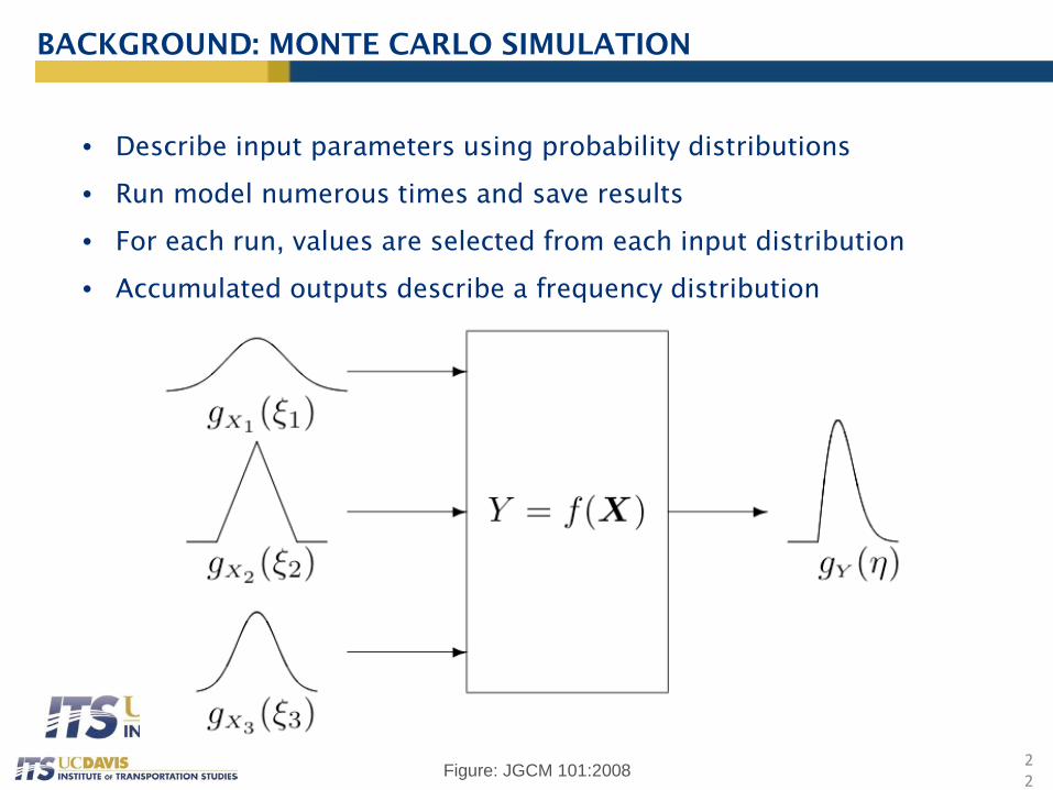
• Describe input parameters using probability distributions

• Run model numerous times and save results

• For each run, values are selected from each input distribution

• Accumulated outputs describe a frequency distribution

BACKGROUND: MONTE CARLO SIMULATION

22 Figure: JGCM 101:2008

1. Limited technical know-how

2. Increased complexity

3. Long run-times preclude Monte Carlo analysis

4. Unknown parameter distributions

5. Scenario uncertainty dominates parametric

uncertainty

Barriers to addressing uncertainty

WHY NOT UNCERTAINTY ANALYSIS?

23

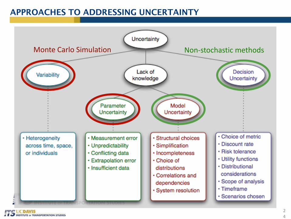
APPROACHES TO ADDRESSING UNCERTAINTY

24

Monte Carlo Simulation Non-stochastic methods

• Generate input parameters

• Run on computing cluster

• Collect results into database

• Analyze results

Features in common with MCS

MONTE CARLO SIMULATION ➡ ROBUST DECISION-MAKING

25

High-speed parallel computing system at NERSC.gov

• Non-probabilistic methods

• PRIM or similar analysis

• Visualization features

Additional requirements

ROBUST DECISION-MAKING

26

• Addresses “deep” uncertainties

– Disagreement about model form, probabilities, value-based judgments

• Focus is robustness rather than optimization or prediction

• Model is used to explore the parameter space

ROBUST DECISION-MAKING: “XLRM” Framework

27

Uncertain Factors (X) Well-defined distributions

Deep uncertainties

Performance metrics (M) Gauge policy performance Single or multiple-attribute

Model relationships (R) Links among Xs, Ls, and Ms

Model equations

Policy Levers (L) Actions that modify the system Potential strategies to explore

Alternative Futures Strategies

Outcomes

Iterate

• Treatment of biofuels

• Indirect effects

• Risk penalty for fuel with uncertain GHG effects

• Feedstock restrictions (waste and residues only)

• Sectoral or economy-wide (e.g., C tax, cap & trade)

• Foresight about ramping cost or targets

• Address path dependence

• Encourage faster behavioral change

• Emphasize RD&D of zero-carbon solutions

Strategies that might be compared in RDM:

REDUCING GHG EMISSIONS FROM TRANSPORTATION

28

GLOBAL CHANGE ANALYSIS MODEL (GCAM)

29 http://prima.pnnl.gov/sites/default/files/Integrated.jpg

• Long Term Shifts in Life Cycle Energy Efficiency and Carbon Intensity Mitigating

• Climate Change: Decomposing the Relative Roles of Energy Conservation, Technological Change and Structural Shift

• Transportation forecasts in various scenarios from IPCC’s SSPs and RCPs (Representative Concentration Pathways or Target Climate Goals)

• International Transportation Modeling Comparison (ITEM)